Workshop on Virtual Reality Interaction and Physical Simulation VRIPHYS (2009)H. Prautzsch, A. Schmitt, J. Bender, M. Teschner (Editors)

Neighboring-based Linear System for Dynamic Meshes

S. Pena Serna1, J. Silva1,2, A. Stork1,3 and A. Marcos2

1Fraunhofer-IGD, Germany2University of Minho, Portugal

3TU-Darmstadt, Germany

delivered by

EUROGRAPHICSEUROGRAPHICS

D LIGITAL IBRARYD LIGITAL IBRARYwww.eg.org diglib.eg.org

AbstractA linear system is a fundamental building block for several mesh-based computer graphics applications suchas simulation, shape deformation, virtual surgery, and fluid/smoke animation, among others. Nevertheless, sucha system is most of the times seen as a black box and algorithms do not deal with its optimization. Dependingon the number of unknowns, the linear system is often considered as an obstacle for real time applicationand as a building block for offline computations. We present in this paper, a neighboring-based methodologyfor representing a linear system. This new representation enables a compact storage of the set of equation,flexibility for ordering the unknowns and a rapid iterative solution, by means of an optimized matrix-vectormultiplication. In addition, this representation facilitates the modification of part of the linear system withoutaffecting its unchanged part and avoiding the complete rebuild of the system. This specially benefits applicationsdealing with dynamic meshes, where the geometry, the topology or both are constantly changed. We presentthe capabilities of our methodology in models with different sizes and for different operations, highlighting thedynamic characteristic of the mesh. We believe that several applications in computer graphics could benefit fromour methodology, in order to improve their convergence and their performance, reducing the number of iterationsand the computation time.

Categories and Subject Descriptors (according to ACM CCS): I.3.7 [Computer Graphics]: Three-DimensionalGraphics and Realism—Animation I.6.3 [Simulation and Modeling]: Applications—G.1.3 [Numerical Analysis]:Numerical Linear Algebra—Linear systems

1. Introduction

Computer graphics has become a multidisciplinary commu-nity with a vast variety of research fields. Nowadays it doesnot only deal with graphics and interaction, it also addressesseveral aspects from engineering, physics, mathematics andnumerical analysis, among others. Because of that, othercommunities have been paying attention to the evolution ofcomputer graphics and at the same time, computer graphicsresearchers are adapting techniques from other disciplinesto achieve more interactivity and realism. Although some ofthese adaptations are achieving promising results, there areother techniques which are adopted without major changes,leading to results, but neglecting a higher degree of integra-tion and optimization. These drawbacks are encountered intechniques which are adopted as black boxes, where only

inputs and outputs are considered, without analyzing the in-ternal process.

A linear system is an example of black boxes ap-plied in computer graphics. Several mesh-based algorithmssuch as simulation, shape deformation, virtual surgery, andfluid/smoke animation make use of it without major modifi-cations. These algorithms need to traverse the mesh, in orderto identify the neighborhoods edges-elements and vertices-elements, to define the dependencies of the equations and tobuild the linear system. The same process is done, whenevera change in the geometry and the topology of the mesh oc-curs, increasing the computation time and therefore affectingthe overall performance. Nevertheless, there are techniquesin computer graphics, which could lead to improvements inthis process, by means of representing the linear system in adifferent form, rather than in a matrix form.

c© The Eurographics Association 2009.

DOI: 10.2312/PE/vriphys/vriphys09/095-103

Pena Serna et al. / Linear System for Dynamic Meshes

The exploration of different representation for a linearsystem was motivated by our aim to find an algorithm, whichis able to handle the simulation of dynamic meshes (mesheswith continuous geometrical and topological changes) at in-teractive rates. We first realized that when a local modifi-cation in the geometry of the mesh occurs, a great part ofthe linear system remains unchanged; however the lack ofneighboring information restricts a local modification (up-date) of the system. Additionally if topological changes oc-cur, the system will need to add or remove topological enti-ties, which will imply the addition or removal of equations(rows and columns) in the system respectively. Hence, westarted investigating strategies, which could easy the updateof the set of equations during geometrical and topologicalchanges of the mesh.

This investigation led us to find a neighboring-based rep-resentation of the linear system, which enables a compactstorage of the equations, flexibility for ordering the un-knowns and a rapid iterative solution, by means of an opti-mized matrix-vector multiplication. This new representationwas found by studying different applications within the com-puter graphics community, which provided us some hints re-garding their utilization of this kind of systems. We also ana-lyzed how the discretization methods for physical problemswork, as well as different solvers, aiming at understandingtheir requirements (section 2). This information helped usdeveloping a methodology, which can effectively improvethe build, update and solution of linear systems and whichcan also reduce the consumption of resources (section 3).We implemented the methodology, in order to evaluate andcompare its performance. We tested the capabilities of ourmethodology in models with different sizes and for differ-ent operations, highlighting the dynamic characteristic of themesh (section 4).

2. Related Work

As we stated in the previous section, we started studying dif-ferent techniques in computer graphics such as deformablemodels ( [NMK∗06]), shape modeling ( [ACF∗06]), anima-tion ( [MSJT08]) and simulation ( [BFMF06]), in order tounderstand how linear systems are used within this commu-nity. The study of these techniques revealed us, that linearsystems are used in a classical way and that there are no op-timization procedures to minimize its build time. Hence, wedecided to analyze partial differential equations ( [Lan03])and discretization techniques, particularly the Finite ElementMethod ( [Hug87] and [SG04]), in order to explore the re-quirements for building linear systems.

Additionally, we wanted to understand how the solution ofa linear system is computed, hence we revised the literatureregarding iterative solvers ( [SVDV00]) and specially theconjugate gradient method ( [She94]). Based on this infor-mation, we realized that we need to concentrate in a physicalproblem, since the generated systems could present different

properties concerning symmetry, definiteness, among others,and depending on this properties, there are solvers which arebetter suited than others. Hence, we decided to concentrateour effort in the solid mechanics problem [Bow09] and toinvestigate the build and the solution of the linear system forthis kind of physics.

Augarde et al. [ARS06] explained that in the linear elas-ticity problem, the Galerkin method causes the stiffness ma-trix to be symmetric and positive definite. This fact makesthe Conjugate Gradient Method a suitable solver for the lin-ear system of equations yielded in the linear elasticity prob-lem. Saad and Vorst presented, in [SVDV00], an in-depthhistorical perspective of iterative solutions of linear systemsand they attributed their origin to the work of Gauss in theearly nineteenth century and show how the main contribu-tions over the years led to the iterative solvers we have nowa-days.

The studied related work suggested us, that the ConjugateGradient method is currently the most appropriate solverfor computing the solution of a linear system of equationsin an iterative form and without using a hierarchy of dis-cretizations or adaptivity methods. Hence, we decided to im-plement the Conjugate Gradient Method based on [She94],where he presented a practical explanation on how the Con-jugate Gradient works and also showed the building blocksand its interconnections, i.e. the method of Steepest Descent,the method of Conjugate Directions and finally their rela-tions within the Conjugate Gradient method.

As mentioned before, our work was motivated by our aimto find an algorithm, which is able to handle the simulationof dynamic meshes at interactive rates. The computer graph-ics community has not deeply dealt with the simulation ofchanging meshes, but there are some interesting approaches.Bro-Nielsen ( [BNC96, BN96]) presented the advantages ofcondensed or Fast Finite Elements for deformable modelsin surgery simulation, where only the surface of the vol-umetric model is considered for the simulation. Gissler etal. [GBT07] proposed recently constraint sets for FE mod-els, where topological changes (merging and breaking) ofdeformable tetrahedral meshes are supported, by means ofreplacing mass points by mass portions (in a constraint set)according to the number of incident tetrahedra.

Klinger et al. [KFCO06] developed a fluid animation ap-plication, which requires the remesh of the whole model af-ter every iteration (or mesh change), leading also to a rebuildof the linear system. Von Funck et al. [vFTS06] developedan algorithm for shape deformation based on time-dependentdivergence-free vector fields, for which they need to build alinear system, in order to find the path between steps. Theyalso implemented a remesh step, since the deformation of themesh between steps led to poor quality triangles, which af-fected the convergence of the linear system. Hence, they alsoneed to rebuild the linear system after every remesh step.

There are several algorithms dealing with the simula-

c© The Eurographics Association 2009.

96

Pena Serna et al. / Linear System for Dynamic Meshes

tion of physically-based deformable models. For exampleMezger et al. [MTPS08] proposed a real time physically-based shape editing algorithm based on the simulation ofthe mechanical properties of the model with a Finite Ele-ment Method discretization. However they used computingmeshes with few tetrahedral elements (up to 1500) and therebuild of the linear system (for every geometry change, thetopology is constant) did not cause any performance prob-lem. These kinds of simulations with bigger meshes (around10.000 tetrahedral elements) will not achieve real time per-formance.

We believe that several applications in computer graph-ics could benefit from our methodology, in order to improvetheir convergence and their performance, reducing the num-ber of iterations and the computation time. The methodologyproposed in this paper, will specially contribute to the rapidsimulation of dynamic meshes. To the best of our knowl-edge, there are no investigations in the same direction as theproposed in this paper. There have been made several ef-forts regarding the improvement of solvers, either with newmethods or with parallelization techniques on the CPU orthe GPU, but there is not enough information about the in-telligent handling and processing of linear systems.

3. Methodology

The algorithm, which we are proposing, aims at effectivelybuilding, updating and solving linear systems, by means ofreducing the processing time and of minimizing the memoryconsumption. A linear system represented in the matrix formis:

Ax = b (1)

where A is the matrix of coefficients, x is the vector of un-knowns and b is the vector of solutions. Based on the studyof the related work, we have understood the objective of thissystem in getting the solution of the problem. The matrix ofcoefficients aims at collecting the information for the equa-tions regarding the connectivity of the vertices (edge topol-ogy) and of the unknowns (vertices without boundary con-ditions) themselves. The process for building the matrix ofcoefficients is normally based on traversing the given mesh(element by element), in order to identify the neighboringelements, which need to contribute to an edge (non diago-nal positions) or to a vertex (diagonal positions). This pro-cess is expensive and when the geometry and the topologyof mesh is changed, the matrix of coefficients needs to bealso changed.

Hence, we realized that if we could have the informationconcerning the elements around an edge, we could easilycollect and build the information of the non diagonal po-sitions of the linear system. Moreover, if we store the com-puted information for every edge (elements around the edge)

within a small edge matrix, we will have enough flexibilityto modify or recompute only the incident edges to a ver-tex, when the vertex changes, without affecting the rest ofthe linear system. Analogically, we can perform the samestrategy for storing the computed information of the diago-nal positions of the linear system, computing a small diag-onal matrix for every unknown. These two sets of matricesare an equivalent representation of the matrix of coefficients,which we will refer to as the equivalent matrix.

Structure wise, we no longer use the traditional sparse ma-trix ( [SGV05]) to store the matrix of coefficients. Instead,we have divided it into two vectors (see Figure 1 for a visualrepresentation). In one vector we store the edge matrices andon the other we store the diagonal matrices. Every elementof both vectors is a nxn matrix where n is the dimension (1D,2D or 3D) of the problem.

Figure 1: Graphic representation of a matrix of coefficients(left). The same matrix of coefficient represented as theequivalent matrix (left).

The two main characteristics of a matrix of coefficients,sparsity and symmetry, are used by the equivalent matrix tominimize memory consumption: only the nonzero values arestored and only one instance of every edge is stored for ev-ery pair of connected vertices. In order to explain how ouralgorithm uses this characteristics for building the equiva-lent matrix and for the sake of clarity, we have subdividedthe process into three steps:

1. Constructing the needed neighboring information2. Computing the set of edge matrices3. Computing the set of diagonal matrices

These three simple steps enable the minimization of thespace in memory and the reduction of the processing time. Inaddition, the new representation of the matrix of coefficientsallows the flexible handling and modification of individualvertices or edges, without affecting the rest of the matrix.The example mesh shown in Figure 2 will be used in associ-ation with Figure 3 and Figure 4 to accompain the explana-tions given in ’Computing the edge matrices’ and ’Comput-ing the diagonal matrices’ respectively.

c© The Eurographics Association 2009.

97

Pena Serna et al. / Linear System for Dynamic Meshes

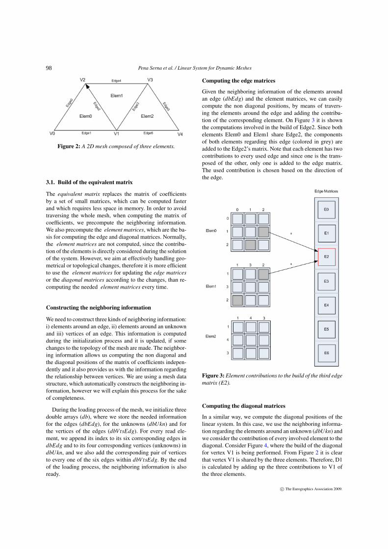
Figure 2: A 2D mesh composed of three elements.

3.1. Build of the equivalent matrix

The equivalent matrix replaces the matrix of coefficientsby a set of small matrices, which can be computed fasterand which requires less space in memory. In order to avoidtraversing the whole mesh, when computing the matrix ofcoefficients, we precompute the neighboring information.We also precompute the element matrices, which are the ba-sis for computing the edge and diagonal matrices. Normally,the element matrices are not computed, since the contribu-tion of the elements is directly considered during the solutionof the system. However, we aim at effectively handling geo-metrical or topological changes, therefore it is more efficientto use the element matrices for updating the edge matricesor the diagonal matrices according to the changes, than re-computing the needed element matrices every time.

Constructing the neighboring information

We need to construct three kinds of neighboring information:i) elements around an edge, ii) elements around an unknownand iii) vertices of an edge. This information is computedduring the initialization process and it is updated, if somechanges to the topology of the mesh are made. The neighbor-ing information allows us computing the non diagonal andthe diagonal positions of the matrix of coefficients indepen-dently and it also provides us with the information regardingthe relationship between vertices. We are using a mesh datastructure, which automatically constructs the neighboring in-formation, however we will explain this process for the sakeof completeness.

During the loading process of the mesh, we initialize threedouble arrays (db), where we store the needed informationfor the edges (dbEdg), for the unknowns (dbUkn) and forthe vertices of the edges (dbVtsEdg). For every read ele-ment, we append its index to its six corresponding edges indbEdg and to its four corresponding vertices (unknowns) indbUkn, and we also add the corresponding pair of verticesto every one of the six edges within dbVtsEdg. By the endof the loading process, the neighboring information is alsoready.

Computing the edge matrices

Given the neighboring information of the elements aroundan edge (dbEdg) and the element matrices, we can easilycompute the non diagonal positions, by means of travers-ing the elements around the edge and adding the contribu-tion of the corresponding element. On Figure 3 it is shownthe computations involved in the build of Edge2. Since bothelements Elem0 and Elem1 share Edge2, the componentsof both elements regarding this edge (colored in grey) areadded to the Edge2’s matrix. Note that each element has twocontributions to every used edge and since one is the trans-posed of the other, only one is added to the edge matrix.The used contribution is chosen based on the direction ofthe edge.

Figure 3: Element contributions to the build of the third edgematrix (E2).

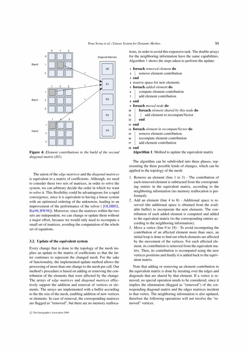
Computing the diagonal matrices

In a similar way, we compute the diagonal positions of thelinear system. In this case, we use the neighboring informa-tion regarding the elements around an unknown (dbUkn) andwe consider the contribution of every involved element to thediagonal. Consider Figure 4, where the build of the diagonalfor vertex V1 is being performed. From Figure 2 it is clearthat vertex V1 is shared by the three elements. Therefore, D1is calculated by adding up the three contributions to V1 ofthe three elements.

c© The Eurographics Association 2009.

98

Pena Serna et al. / Linear System for Dynamic Meshes

Figure 4: Element contributions to the build of the seconddiagonal matrix (D1).

The union of the edge matrices and the diagonal matricesis equivalent to a matrix of coefficients. Although, we needto consider these two sets of matrices, in order to solve thesystem, we can arbitrary decide the order in which we wantto solve it. This flexibility could be advantageous for a rapidconvergence, since it is equivalent to having a linear systemwith an optimized ordering of the unknowns, leading to animprovement of the performance of the solver ( [OLHB02,Bar96,BW98]). Moreover, since the matrices within the twosets are independent, we can change or update them withouta major effort, because we would only need to recompute asmall set of matrices, avoiding the computation of the wholeset of equations.

3.2. Update of the equivalent system

Every change that is done to the topology of the mesh im-plies an update to the matrix of coefficients so that the lat-ter continues to represent the changed mesh. For the sakeof functionality, the implemented update method allows theprocessing of more than one change to the mesh per call. Ourmethod’s procedure is based on adding or removing the con-tribution of the elements that were affected by the change.The arrays of edge matrices and diagonal matrices effec-tively support the addition and removal of vertices or ele-ments. The arrays are implemented with a buffer accordingto the the size of the mesh, enabling addition of new verticesor elements. In case of removal, the corresponding matricesare flagged as “removed”, but there are no memory realloca-

tions, in order to avoid this expensive task. The double arraysfor the neighboring information have the same capabilities.Algorithm 1 shows the steps taken to perform the update:

foreach removed element do1

remove element contribution2

end3

reserve space for new elements4

foreach added element do5

compute element contribution6

add element contribution7

end8

foreach moved node do9

foreach element shared by this node do10

add element to recomputeVector11

end12

end13

foreach element in recomputeVector do14

remove element contribution15

recompute element contribution16

add element contribution17

end18

Algorithm 1: Method to update the equivalent matrix

The algorithm can be subdivided into three phases, rep-resenting the three possible kinds of changes, which can beapplied to the topology of the mesh:

1. Remove an element (line 1 to 3) - The contribution ofeach removed element is subtracted from the correspond-ing entries in the equivalent matrix, according to theneighboring information (no memory reallocation is per-formed);

2. Add an element (line 4 to 8) - Additional space is re-served (the additional space is obtained from the avail-able buffer) to incorporate the new elements. The con-tribution of each added element is computed and addedto the equivalent matrix (to the corresponding entries ac-cording to the neighboring information);

3. Move a vertex (line 9 to 18) - To avoid recomputing thecontribution of an affected element more than once, aninitial loop is done to find out which elements are affectedby the movement of the vertices. For each affected ele-ment, its contribution is removed from the equivalent ma-trix. Then, its contribution is recomputed using the newvertices positions and finally it is added back to the equiv-alent matrix.

Note that adding or removing an element contribution tothe equivalent matrix is done by iterating over the edges anddiagonals that are shared by that element. If a vertex is re-moved, no special operation needs to be considered, since itimplies the elimination (flagged as “removed”) of the cor-responding diagonal matrix and the edges matrices incidentto that vertex. The neighboring information is also updated,therefore the following operations will not involve the “re-moved” vertices.

c© The Eurographics Association 2009.

99

Pena Serna et al. / Linear System for Dynamic Meshes

3.3. Solution of the equivalent system

The implemented algorithm to solve the linear system ofequations is the Conjugate Gradient as it was proposed in[She94]. The only noticeable change done so far is the waywe multiply the equivalent matrix with a vector. Although,we have chosen the Conjugate Gradient method for solvingthe linear system, our methodology is completely indepen-dent of the kind of solver. Our algorithm is suitable for otheriterative methods or even direct methods.

Multiplication of the equivalent matrix with a vector

Having the matrix of coefficients stored in the equivalentmatrix form requires a special method for its multiplicationwith a vector.

foreach rst in resultVector do1

resultVector[rst] = 02

end3

foreach edge in edgeVector do4

edgeStartVertex = start vertex of this edge5

edgeEndVertex = end vertex of this edge6

resultVector += (edgeVector[edge] * multiVector)7

resultVector += (edgeVector[edge]T * multiVector)8

end9

foreach diag in diagVector do10

resultVector += (diagVector[diag] * multiVector)11

end12

Algorithm 2: Multiplication of the equivalent matrix witha vector (multiVector) and its result (resultVector).

Algorithm 2 shows the main steps we perform to multi-ply the equivalent matrix with a vector. We start by settingthe resultVector to zero so that the results of the multiplica-tions performed over the matrix can be added to it. For everyedge, we find the vertices that form that edge (edgeStartVer-tex and edgeEndVertex) by consulting the neighborhood in-formation (dbVtsEdg). This is done to know which is thisedge position in the matrix. Doing so it is known with whichposition of multiVector this edge should be multiplied andin what position of resultVector it should be stored.

Also notice that for every edge two multiplications aredone. This is due to the symmetric characteristic of the ma-trix. To provide a better understanding of this procedure con-sider the example shown in Figure 5. Assuming that we areiterating on edge E1 and that this edge has vertex 0 as a start-ing vertex and vertex 3 as an ending vertex. In line 7 of thealgorithm we would multiply E1 by V3 and store its resultin R0 (red boxes). And since E1 also connect vertex 3 tovertex 0 with the same value, in line 8 we store in R3 themultiplication of the transposed E1 with V0 (green boxes).

After processing all the edges, we iterate on the diagonals.The process is similar but simpler, for each diagonal relatesa vertex to itself.

Figure 5: Multiplication of the equivalent matrix (repre-sented as a normal matrix for simplification) with a vector.The green and red line colored boxes indicate the used val-ues when the multiplication iterates on edge E1.

4. Results

We have implemented the build of the equivalent matrix(DEM) and its multiplication with a vector , as proposedin the previous section. This implementation is not complexand it can easily be reproduced following the given indica-tions. Our implementation is single threading and a desk-top PC Intel Core 2 Quad Q6600 with 3.25 GB RAM wasused to make the measurements. In order to compare theperformance of our algorithm, we have also implementedthe classical form to represent the matrix of coefficients, thesparse matrix. We programmed four implementations of thesparse matrix: i) linked lists without the symmetric charac-teristic (CSM), ii) linked lists with the symmetric character-istic (SSM), iii) compressed row storage (CRS) and iv) blockcompressed row storage (BCRS).

The first two implementations (CSM and SSM) were onlymade for the sake of completeness, hence a simple arrayof linked lists was employed. The last two implementations(CRS and BCRS) were done without considering the sym-metric characteristic, since we wanted faster access duringthe multiplication of the matrix with a vector (SPMV). Theimplementation of the multiplication with a vector was madefor the four representations as well. For the build process ofCSM, SSM, CRS, and BCRS, we have used the neighboringinformation, in other words, we store the needed informationin the representation without traversing the whole mesh. Forthe multiplication process, the neighboring information wasnot used for CSM, SSM, CRS and BCRS, since each one hasfields for identifying the corresponding position in the mesh.

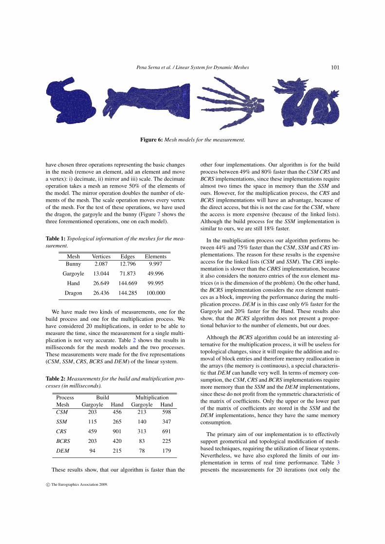
In order to measure the performance of the five implemen-tations, we have used two different tetrahedral meshes: i) agargoyle with almost 50.000 elements and ii) a hand withalmost 100.000 elements. Table 1 presents the relevant topo-logical information of the meshes (shown in Figure 6). Inorder to present the capabilities of the update process, we

c© The Eurographics Association 2009.

100

Pena Serna et al. / Linear System for Dynamic Meshes

Figure 6: Mesh models for the measurement.

have chosen three operations representing the basic changesin the mesh (remove an element, add an element and movea vertex): i) decimate, ii) mirror and iii) scale. The decimateoperation takes a mesh an remove 50% of the elements ofthe model. The mirror operation doubles the number of ele-ments of the mesh. The scale operation moves every vertexof the mesh. For the test of these operations, we have usedthe dragon, the gargoyle and the bunny (Figure 7 shows thethree forementioned operations, one on each model).

Table 1: Topological information of the meshes for the mea-surement.

Mesh Vertices Edges ElementsBunny 2.087 12.796 9.997

Gargoyle 13.044 71.873 49.996

Hand 26.649 144.669 99.995

Dragon 26.436 144.285 100.000

We have made two kinds of measurements, one for thebuild process and one for the multiplication process. Wehave considered 20 multiplications, in order to be able tomeasure the time, since the measurement for a single multi-plication is not very accurate. Table 2 shows the results inmilliseconds for the mesh models and the two processes.These measurements were made for the five representations(CSM, SSM, CRS, BCRS and DEM) of the linear system.

Table 2: Measurements for the build and multiplication pro-cesses (in milliseconds).

Process Build MultiplicationMesh Gargoyle Hand Gargoyle HandCSM 203 456 213 598

SSM 115 265 140 347

CRS 459 901 313 691

BCRS 203 420 83 225

DEM 94 215 78 179

These results show, that our algorithm is faster than the

other four implementations. Our algorithm is for the buildprocess between 49% and 80% faster than the CSM CRS andBCRS implementations, since these implementations requirealmost two times the space in memory than the SSM andours. However, for the multiplication process, the CRS andBCRS implementations will have an advantage, because ofthe direct access, but this is not the case for the CSM, wherethe access is more expensive (because of the linked lists).Although the build process for the SSM implementation issimilar to ours, we are still 18% faster.

In the multiplication process our algorithm performs be-tween 44% and 75% faster than the CSM, SSM and CRS im-plementations. The reason for these results is the expensiveaccess for the linked lists (CSM and SSM). The CRS imple-mentation is slower than the CBRS implementation, becauseit also considers the nonzero entries of the nxn element ma-trices (n is the dimension of the problem). On the other hand,the BCRS implementation considers the nxn element matri-ces as a block, improving the performance during the multi-plication process. DEM is in this case only 6% faster for theGargoyle and 20% faster for the Hand. These results alsoshow, that the BCRS algorithm does not present a propor-tional behavior to the number of elements, but our does.

Although the BCRS algorithm could be an interesting al-ternative for the multiplication process, it will be useless fortopological changes, since it will require the addition and re-moval of block entries and therefore memory reallocation inthe arrays (the memory is continuous), a special characteris-tic that DEM can handle very well. In terms of memory con-sumption, the CSM, CRS and BCRS implementations requiremore memory than the SSM and the DEM implementations,since these do not profit from the symmetric characteristic ofthe matrix of coefficients. Only the upper or the lower partof the matrix of coefficients are stored in the SSM and theDEM implementations, hence they have the same memoryconsumption.

The primary aim of our implementation is to effectivelysupport geometrical and topological modification of mesh-based techniques, requiring the utilization of linear systems.Nevertheless, we have also explored the limits of our im-plementation in terms of real time performance. Table 3presents the measurements for 20 iterations (not only the

c© The Eurographics Association 2009.

101

Pena Serna et al. / Linear System for Dynamic Meshes

multiplication) of the conjugate gradient method with a Ja-cobi preconditioner for three meshes with different sizes.

Table 3: Meshes with real time performance (time in mil-liseconds).

Mesh Vertices Elements Time FPSBunny_10 2.087 9997 16 63

Gargoyle_30 7.944 29.998 47 21

Gargoyle_50 13.044 49.996 99 10

These results reveal that our algorithm can perform inreal time with meshes up to 30.000 elements and at interac-tive rates with meshes up to 50.000 elements. As mentionedabove, our algorithms aims at effectively handling geometri-cal and topological changes. Because of that, we store thepre-computation of the element matrices, in order to eas-ily update the equivalent system, whenever a change in thetopology (remove or add vertices and elements) or in the ge-ometry (move vertices) happen. The three implemented op-erations (decimate, mirror and scale) are extreme examples,since they employ at least the 50% of the elements or the ver-tices and this is not a common activity in computer graphics,where fast performance is expected.

The decimate operation removes half of the elements ofthe model, hence only the elements, which are on the bound-ary of the removal are recomputed (see table 4). Since theelements on the boundary of the removal are much less thanhalf of the model, the update process is much faster than thereconstruction.

Table 4: Measurements for the decimate operation (in mil-liseconds).

Mesh Initialization Update ReconstructionBunny 140 < 1 67

Gargoyle 702 71 359

Dragon 1.427 47 719

The update process for the mirror operation takes approx-imately 50% of the time of the reconstruction (see table 5),because it only processes the mirrored elements in compar-ison with the reconstruction, which processes two times thenumber of elements (the original and the mirrored ones).

The update process for the scale operation takes slightlymore time than the reconstruction (see table 6), howevermoving the complete set of vertices in a single step is theworst case scenario, thus any other operation involving mov-ing vertices will perform much faster than the reconstruc-tion.

The presented three operations show the performance ofour algorithm for geometrical and topological changes. We

Table 5: Measurements for the mirror operation (in millisec-onds).

Mesh Initialization Update ReconstructionBunny 140 125 276

Gargoyle 702 783 1.416

Dragon 1.427 1.380 2.857

Table 6: Measurements for the scale operation (in millisec-onds).

Mesh Initialization Update ReconstructionBunny 140 140 141

Gargoyle 702 736 703

Dragon 1.427 1.483 1.427

demonstrated that our algorithm is in normal conditions (noextreme examples) much faster than a complete reconstruc-tion of the linear system. This is an improvement towardsmesh-based applications such as simulation, shape deforma-tion, virtual surgery, and fluid/smoke animation, among oth-ers, where geometrical (and sometimes topological) changesaffect the linear system, which needs to be solved. Thesekinds of applications will not only benefit from faster up-dates, but also from faster solutions, as demonstrated withthe multiplication process.

Hence, our methodology enables interactive rates for dy-namic meshes with up to 50.000 elements in a single thread.From the previous results, we have also realized that theproposed algorithms behave proportional to the size of themeshes. In other words, the complexity of the algorithms isO(n).

5. Conclusions and future work

We have presented algorithms, which use the neighboring in-formation of the mesh to effectively build, update and solvelinear systems. Our algorithms avoid the assembly of the ma-trix of coefficients and they also reduce the processing timeand the memory consumption. The proposed methodologyalso enables the handling of the set of equations with moreflexibility, allowing their iteration and solution in any arbi-trary order. We have started the exploration of this aspectand we are evaluating different alternatives, for example:reverse Cuthill-McKee (RCM), self-avoiding walk (SAW),out-in ordering (ordering from the boundary to the interior)or multi layer solving. The last three options are based onthe neighboring information of the mesh, a characteristic,which we have also exploited in this paper. This flexibilityis a step forward towards the simulation of meshes with dy-namic topology or dynamic meshes. We will further imple-ment and refine our algorithms, we want to explore other

c© The Eurographics Association 2009.

102

Pena Serna et al. / Linear System for Dynamic Meshes

Figure 7: From left to right: decimated bunny, mirrored gargoyle and scaled dragon.

iterative solvers and we have already strated with a directsolver (Cholesky factorization). We want also to investigateparallelization schemes, either for the CPU or the GPU. Wealso plan to develop a framework, where the modificationof meshes and its real time simulation will be feasible, aim-ing at integrating design and analysis of mechanical objectswithin the same environment.

6. Aknowledgement

This work is partially supported by the European projects3D-COFORM (FP7-ICT-2007.4.3-231809) and FOKUSK3D (FP7-ICT-2007-214993).

References

[ACF∗06] ALEXA M., CANI M.-P., FRISKEN S., SINGH K.,SCHKOLNE S., ZORIN D.: Interactive Shape Editing: SIG-GRAPH 2006 course notes. In SIGGRAPH ’06: ACM SIG-GRAPH 2006 Courses (2006), ACM New York, NY, USA. 2

[ARS06] AUGARDE C., RAMAGE A., STAUDACHER J.: Anelement-based displacement preconditioner for linear elasticityproblems. Computers and structures 84, 31-32 (2006), 2306–2315. 2

[Bar96] BARAFF D.: Linear-time dynamics using lagrange mul-tipliers. In SIGGRAPH ’96: Proceedings of the 23rd annual con-ference on Computer graphics and interactive techniques (NewYork, NY, USA, 1996), ACM, pp. 137–146. 5

[BFMF06] BRIDSON R., FEDKIW R., MULLER-FISCHER M.:Fluid simulation: Siggraph 2006 course notes. In SIGGRAPH’06: ACM SIGGRAPH 2006 Courses (New York, NY, USA,2006), ACM, pp. 1–87. 2

[BN96] BRO-NIELSEN M.: Surgery simulation using fast finiteelements. In VBC ’96: Proceedings of the 4th International Con-ference on Visualization in Biomedical Computing (London, UK,1996), Springer-Verlag, pp. 529–534. 2

[BNC96] BRO-NIELSEN M., COTIN S.: Real-time volumetricdeformable models for surgery simulation using finite elementsand condensation. In Computer Graphics Forum (1996), pp. 57–66. 2

[Bow09] BOWER A.: Applied Mechanics of Solids, 1 ed. Taylorand Francis, August 2009. 2

[BW98] BARAFF D., WITKIN A.: Large steps in cloth simula-tion. In Proceedings of the 25th annual conference on Computergraphics and interactive techniques (1998), ACM New York, NY,USA, pp. 43–54. 5

[GBT07] GISSLER M., BECKER M., TESCHNER M.: Constraintsets for topology-changing finite element models. In Virtual Re-ality Interactions and Physical Simulations VRIPHYS (Novem-ber 9 2007), pp. 21–26. 2

[Hug87] HUGHES T.: The finite element method: linear static anddynamic finite element analysis. Prentice-Hall Englewood Cliffs,NJ, 1987. 2

[KFCO06] KLINGNER B. M., FELDMAN B. E., CHENTANEZN., O’BRIEN J. F.: Fluid Animation with Dynamic Meshes. InInternational Conference on Computer Graphics and InteractiveTechniques (2006), ACM New York, NY, USA. 2

[Lan03] LANGTANGEN H.: Computational partial differen-tial equations: numerical methods and diffpack programming.Springer Berlin, 2003. 2

[MSJT08] MÜLLER M., STAM J., JAMES D., THÜREY N.: Realtime physics: class notes. In International Conference on Com-puter Graphics and Interactive Techniques (2008), ACM NewYork, NY, USA. 2

[MTPS08] MEZGER J., THOMASZEWSKI B., PABST S.,STRASSER W.: Interactive Physically-Based Shape Editing. InACM Solid and Physical Modeling Symposium (SPM) (2008). 3

[NMK∗06] NEALEN A., MÜLLER M., KEISER R., BOXERMANE., CARLON M.: Physically Based Deformable Models in Com-puter Graphics. Computer Graphics Forum 25, 4 (2006), 809–836. 2

[OLHB02] OLIKER L., LI X., HUSBANDS P., BISWAS R.: Ef-fects of ordering strategies and programming paradigms onsparse matrix computations. SIAM Review 44, 3 (2002), 373–393. 5

[SG04] SMITH I., GRIFFITHS D.: Programming the finite elementmethod. Wiley, 2004. 2

[SGV05] SMAILBEGOVIC F., GAYDADJIEV G. N., VASSIL-IADIS S.: Sparse matrix storage format. In Proceedings of the16th Annual Workshop on Circuits, Systems and Signal Process-ing, ProRisc 2005 (November 2005), pp. 445–448. 3

[She94] SHEWCHUK J.: An introduction to the conjugate gradi-ent method without the agonizing pain. Computer Science Tech.Report (1994), 94–125. 2, 6

[SVDV00] SAAD Y., VAN DER VORST H.: Iterative solution oflinear systems in the 20th century. Journal of Computational andApplied Mathematics 123, 1-2 (2000), 1–33. 2

[vFTS06] VON FUNCK W., THEISEL H., SEIDEL H. P.: VectorField Based Shape Deformations. In International Conferenceon Computer Graphics and Interactive Techniques (2006), ACMNew York, NY, USA. 2

c© The Eurographics Association 2009.

103