Applied Numerical Mathematics 59 (2009) 723–738

www.elsevier.com/locate/apnum

The continuous extension of the B-spline linear multistep methodsfor BVPs on non-uniform meshes

Francesca Mazzia a, Alessandra Sestini b,∗, Donato Trigiante c

a Dipartimento di Matematica, Via Orabona 4, 70125 Bari, Italyb Dipartimento di Matematica U. Dini, V.le Morgagni 67/A, 50134 Firenze, Italyc Dipartimento di Energetica S. Stecco, Via Lombroso 6/17, 50134 Firenze, Italy

Available online 8 April 2008

Abstract

B-spline methods are Linear Multistep Methods based on B-splines which have good stability properties [F. Mazzia, A. Sestini,D. Trigiante, B-spline multistep methods and their continuous extensions, SIAM J. Numer Anal. 44 (5) (2006) 1954–1973] whenused as Boundary Value Methods [L. Brugnano, D. Trigiante, Convergence and stability of boundary value methods for ordinarydifferential equations, J. Comput. Appl. Math. 66 (1–2) (1996) 97–109; L. Brugnano, D. Trigiante, Solving Differential Problemsby Multistep Initial and Boundary Value Methods, Gordon and Breach Science Publishers, Amsterdam, 1998]. In addition, theyhave an important feature: if k is the number of steps, it is always possible to associate to the numerical solution a Ck spline ofdegree k + 1 collocating the differential equation at the mesh points. In this paper we introduce an efficient algorithm to computethis continuous extension in the general case of a non-uniform mesh and we prove that the spline shares the convergence orderwith the numerical solution. Some numerical results for boundary value problems are presented in order to show that the use of theinformation given by the continuous extension in the mesh selection strategy and in the Newton iteration makes more robust andefficient a Matlab code for the solution of BVPs.© 2008 IMACS. Published by Elsevier B.V. All rights reserved.

MSC: 65L06; 65L10; 65D07; 41A15

Keywords: Boundary value problems; Ordinary differential equations; B-splines; Spline collocation; Boundary value methods; Continuousextensions

1. Introduction

B-spline methods (for brevity referred to in the following as BS methods) are a class of Linear Multistep Methods(LMMs) based on B-Splines [13,14], which can be used to solve numerically the following general Boundary ValueProblem (BVP):{

y′(x) = f(x,y(x)

), a � x � b,

g(y(a),y(b)

) = 0,(1)

* Corresponding author.E-mail addresses: mazzia@dm.uniba.it (F. Mazzia), sestini@math.unifi.it (A. Sestini), trigiant@unifi.it (D. Trigiante).

0168-9274/$30.00 © 2008 IMACS. Published by Elsevier B.V. All rights reserved.doi:10.1016/j.apnum.2008.03.036

724 F. Mazzia et al. / Applied Numerical Mathematics 59 (2009) 723–738

where y ∈ Rd , d � 1 and f and g are sufficiently smooth functions. The stability features of these methods for uniform

meshes have been studied in [13], where it is shown that they have to be used as BVMs, that is combined with asuitable number of initial and final additional methods. It is worth recalling here that a k-step method requires k

conditions. One of them is inherited from the continuous problem (i.e. the second condition in (1)); the others, calledadditional, can be all placed at the initial point (IVM use) or appropriately split between the initial and the final point(BVM use, see [2] and [3] for a general introduction). Their convergence has been studied in [13] for uniform meshesand in [14] for the general case. In [14] the mathematical characterization of their coefficients for non-uniform meshesis also introduced, together with an algorithm for their numerical computation. In [13], dealing with uniform meshes,it was proved that an important feature of the BS methods is that, if k is the number of steps, it is always possible tocompute a polynomial spline of degree k + 1 and smoothness Ck, collocating the differential equation at the meshpoints. Here we prove that this feature is preserved when non-uniform meshes are considered and, in particular, it isshown that such spline shares the convergence order with the numerical solution. In addition, an efficient algorithmfor the computation of the spline coefficients is introduced.

From a practical point of view, the possibility to associate with the numerical solution a continuous extension withthe same accuracy can make more robust any mesh selection strategy and becomes particularly interesting when non-linear problems are dealt with. Any step variation strategy, see, e.g., [16], requires an approximation of the error thatcan be obtained either considering only the numerical solution at the mesh points or using a continuous extension.Moreover, the approximation of the solution at off–mesh points is also required by the quasi-linearization technique.Clearly, if this approximation is poor the whole process is compromised and in some cases (in particular when difficultnon-linear problems are considered) convergence can be lost. In this paper we show how the use of the spline extensionassociated with the BS methods can be useful for improving the performance of the whole algorithm.

After introducing in Section 2 the BS methods and their main properties, in Section 3 we prove that there alwaysexists a unique k+1 degree Ck spline with knots at the mesh points which extends continuously the numerical solutionand collocates the differential equation at the mesh points. In the same section a new and efficient algorithm for thecomputation of its coefficients in the B-spline basis is also introduced and the spline approximation order is studied;we show that the convergence order of the spline is consistent with the order of the numerical solution at the meshpoints. In Section 4 two possible uses of the information given by the continuous extension are presented in order toimprove both the mesh selection and the quasi-linearization techniques. Finally, in Section 5, some numerical resultsare reported.

2. BS methods

The BS methods are linear multistep methods to be used as Boundary Value Methods [3] in order to ensure theirconvergence and good stability behavior. Thus, if

π = {a = x0 < x1 < · · · < xN = b}is a mesh in the integration interval [a, b], the associated numerical solution {yi , i = 0, . . . ,N} of (1) (whereyi ≈ y(xi)) produced by the k-step BS method is defined by the following equations,⎧⎪⎪⎪⎪⎪⎪⎪⎪⎪⎪⎪⎪⎪⎪⎪⎪⎪⎪⎨

⎪⎪⎪⎪⎪⎪⎪⎪⎪⎪⎪⎪⎪⎪⎪⎪⎪⎪⎩

g(y0,yN) = 0,

k−i∑j=−i

α(i)j+iyi+j = hi

k−i∑j=−i

β(i)j+ifi+j , i = 1, . . . , k1 − 1,

(additional initial methods)k2∑

j=−k1

α(i)j+k1

yi+j = hi

k2∑j=−k1

β(i)j+k1

fi+j , i = k1, . . . ,N − k2,

(main methods)N−i∑

j=N−i−k

α(i)j−N+i+kyi+j = hi

N−i∑j=N−i−k

β(i)j−N+i+kfi+j , i = N + 1 − k2, . . . ,N,

(2)

(additional final methods)

F. Mazzia et al. / Applied Numerical Mathematics 59 (2009) 723–738 725

where hi := xi − xi−1, fl := f(xl,yl) and where α(i) = (α(i)0 , . . . , α

(i)k )T and β(i) = (β

(i)0 , . . . , β

(i)k )T , i = k1, . . . ,

N − k2, are the coefficient vectors characterizing the main method. As follows from the linear stability analysis [13],the k-step BS method is correctly used if it is combined with k1 − 1 left and k2 right additional methods, wherek1 := � k

2� and k2 := � k2. Concerning the additional methods, we outline that, as in the case for spline interpolation,

several choices are possible, because the only requirement is that their order is at least p − 1, if p is the order of themain scheme. A possible choice, already introduced in [14], will be used later in Section 5.

In the case of uniform meshes the vectors α(i) and β(i) of the main methods do not depend on i and they assumethe following easy form,

αj := B ′(k − j + 1), βj := B(k − j + 1), j = 0, . . . , k,

where B(x) is the k + 1 degree B-spline with integer knots 0, . . . , k + 2 [6].In the general non-uniform case, each couple of vectors α(i) and β(i), i = k1, . . . ,N − k2, has to be computed bysolving a linear system of size (2k + 2) × (2k + 2). The entries of the related coefficient matrix depend on the valuesof 2k+1 successive B-spline functions and of their derivatives computed at successive k+1 mesh points, as discussedin details in [14]. Since the same coefficient matrices will be used in the next section to compute the spline extension,we report here such linear systems, after the introduction of few necessary facts about B-splines.

Let Sk,N be the set of all Ck polynomial splines of degree k + 1 defined in [a, b] with knots x0, . . . , xN whosedimension is N + k + 1. We represent any s ∈ Sk,N in the k + 1 degree B-spline basis Bi(x), i = −(1 + k), . . . ,N − 1,which can be defined after prescribing 2 sets of additional (k + 1) knots, {xi, i = −(1 + k), . . . ,−1} (left auxiliaryknots), with x−1−k � · · · � x0, and {xi, i = N + 1, . . . ,N + k + 1} (right auxiliary knots), with xN � xN+1 � · · · �xN+k+1 [6]. Thus we can write Sk,N = 〈B−(1+k), . . . ,BN−1〉. The two vectors α(i) and β(i) ∈ R

k+1 are defined as thesolution of the following linear system,

G(i)(α(i)T ,β(i)T

)T = e2k+2, (3)

where e2k+2 = (0, . . . ,0,1)T ∈ R2k+2 and

G(i) :=[

A(i−k1)T1 −hiA

(i−k1)T2

0T eT

], (4)

with e := (1, . . . ,1)T ∈ Rk+1, and A

(j)

1 ,A(j)

2 , j ∈ N, defined as,

A(j)

1 :=⎡⎣ Bj−k−1(xj ), . . . , Bj+k−1(xj )

......

...

Bj−k−1(xj+k), . . . , Bj+k−1(xj+k)

⎤⎦

(k+1)×(2k+1)

,

A(j)

2 :=⎡⎢⎣

B ′j−k−1(xj ), . . . , B ′

j+k−1(xj )

......

...

B ′j−k−1(xj+k), . . . , B ′

j+k−1(xj+k)

⎤⎥⎦

(k+1)×(2k+1)

.

In [14] the non-singularity of G(i) was proved and, moreover, an efficient and accurate technique for solving (3)was introduced.

Remark. It is well know that the stability of multistep methods is influenced by the use of variable stepsize. In [9,10]the effect of the use of variable stepsizes with the variable step technique (the same used to define the coefficients ofour BS methods) is analyzed. The conclusion is that the technique is stable when the rate of change of sizes is small,that is the mesh is locally quasi-uniform. Since we would like to preserve the stability condition proved for fixedstepsize, we implement the numerical scheme using locally quasi-uniform meshes, which means that there exists apositive constant rπ � 1 such that,

1/rπ < hi/hi+1 < rπ . (5)

726 F. Mazzia et al. / Applied Numerical Mathematics 59 (2009) 723–738

2.1. The linear case

When (1) is linear, the discrete problem (2) arising using the BS-method is a linear system of size d(N + 1) ×d(N + 1). In fact, in this case, (1) can be written as follows{

y′(x) = J(x)y(x) + v(x), a � x � b,

Cay(a) + Cby(b) = w,(6)

where Ca and Cb are constant matrices of size d × d, J(x) is a matrix of size d × d , defined in [a, b], w is a givenvector in R

d and v(x) is an assigned vector function defined in [a, b]. Using the BS method with k steps (and orderp = k + 1) on the mesh π , the discrete solution Y(p) := (yT

0 , . . . ,yTN)T of (2) is the solution of the following linear

system,

MpY(p) = e1 ⊗ w + BpV, (7)

where e1 := (1,0, . . . ,0)T ∈ RN+1, V := (v(x0)

T , . . . ,v(xN)T )T and

Mp := Ap − BpJ (8)

with J := diag(J(x0), . . . ,J(xN)) and

Ap :=(Ca 0d,d(N−1) Cb

Ap ⊗ Id

), Bp :=

(0d,d(N+1)

(HBp) ⊗ Id

), (9)

where H := diag(h1, . . . , hN) and Ap and Bp are banded matrices of size N × (N +1) defined using all the coefficientsof the main method and of the additional methods. In particular, when k1 � i � N −k2, in the i-th row of the matrix Ap

(Bp) there is the vector α(i)T , (β(i)T ) (and it is located between the (i +1− k1)-th and the (i + k2 +1)-th columns). Inthe k1 − 1 initial and in the k2 final rows of these matrices there are the α and β coefficients of the additional methods,respectively. We consider the non-linear case in Section 4.

3. The spline extension

In this section we first show that there always exists a unique spline sk(x) ∈ Sdk,N := Sk,N ⊗ · · · ⊗ Sk,N︸ ︷︷ ︸

d

extending

the numerical solution {yi , i = 0, . . . ,N} computed by the k-step BS method and collocating the differential equationat the mesh points. Then we introduce a new algorithm to compute efficiently its coefficients in the B-spline basis andwe prove that it has the same order of convergence as the numerical solution.

3.1. Existence and uniqueness

We look for a spline sk(x) ∈ Sdk,N satisfying the following requirements,{

sk(xi) = yi , i = 0, . . . ,N,

s′k(xi) = fi , i = 0, . . . ,N.

(10)

Thus, using the B-spline representation,

sk(x) =N−1∑

i=−(1+k)

ciBi(x), x ∈ [a, b], (11)

(ci ∈ Rd , i = −(1 + k), . . . ,N − 1), (10) can be re-written in the following compact matrix form,

(A ⊗ Id)c = (yT

0 , . . . ,yTN , fT0 , . . . , fTN

)T, (12)

where c = (cT−(1+k), . . . , cT

N−1)T ∈ R

d(N+k+1), Id is the identity matrix of size d × d and A := (AT1 ,AT

2 )T , with A1

and A2 (k + 1)-banded matrices both of size (N + 1) × (N + k + 1) with entries defined as follows

(A1)i,j := Bj (xi), (A2)i,j := B ′j (xi). (13)

F. Mazzia et al. / Applied Numerical Mathematics 59 (2009) 723–738 727

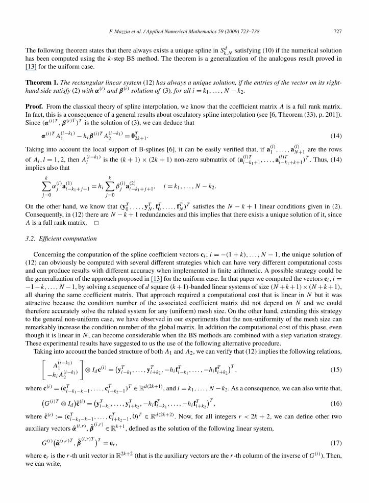
The following theorem states that there always exists a unique spline in Sdk,N satisfying (10) if the numerical solution

has been computed using the k-step BS method. The theorem is a generalization of the analogous result proved in[13] for the uniform case.

Theorem 1. The rectangular linear system (12) has always a unique solution, if the entries of the vector on its right-hand side satisfy (2) with α(i) and β(i) solution of (3), for all i = k1, . . . ,N − k2.

Proof. From the classical theory of spline interpolation, we know that the coefficient matrix A is a full rank matrix.In fact, this is a consequence of a general results about osculatory spline interpolation (see [6, Theorem (33), p. 201]).Since (α(i)T ,β(i)T )T is the solution of (3), we can deduce that

α(i)T A(i−k1)1 − hiβ

(i)T A(i−k1)2 = 0T

2k+1. (14)

Taking into account the local support of B-splines [6], it can be easily verified that, if a(l)1 , . . . ,a(l)

N+1 are the rows

of Al, l = 1,2, then A(i−k1)l is the (k + 1) × (2k + 1) non-zero submatrix of (a(l)T

i−k1+1, . . . ,a(l)Ti−k1+k+1)

T . Thus, (14)implies also that

k∑j=0

α(i)j a(1)

i−k1+j+1 = hi

k∑j=0

β(i)j a(2)

i−k1+j+1, i = k1, . . . ,N − k2.

On the other hand, we know that (yT0 , . . . ,yT

N , fT0 , . . . , fTN)T satisfies the N − k + 1 linear conditions given in (2).Consequently, in (12) there are N − k + 1 redundancies and this implies that there exists a unique solution of it, sinceA is a full rank matrix. �3.2. Efficient computation

Concerning the computation of the spline coefficient vectors ci , i = −(1 + k), . . . ,N − 1, the unique solution of(12) can obviously be computed with several different strategies which can have very different computational costsand can produce results with different accuracy when implemented in finite arithmetic. A possible strategy could bethe generalization of the approach proposed in [13] for the uniform case. In that paper we computed the vectors ci , i =−1−k, . . . ,N −1, by solving a sequence of d square (k+1)-banded linear systems of size (N +k+1)× (N +k+1),all sharing the same coefficient matrix. That approach required a computational cost that is linear in N but it wasattractive because the condition number of the associated coefficient matrix did not depend on N and we couldtherefore accurately solve the related system for any (uniform) mesh size. On the other hand, extending this strategyto the general non-uniform case, we have observed in our experiments that the non-uniformity of the mesh size canremarkably increase the condition number of the global matrix. In addition the computational cost of this phase, eventhough it is linear in N , can become considerable when the BS methods are combined with a step variation strategy.These experimental results have suggested to us the use of the following alternative procedure.

Taking into account the banded structure of both A1 and A2, we can verify that (12) implies the following relations,[A

(i−k1)1

−hiA(i−k1)2

]⊗ Idc(i) = (

yTi−k1

, . . . ,yTi+k2

,−hifTi−k1, . . . ,−hifTi+k2

)T, (15)

where c(i) = (cTi−k1−k−1, . . . , cT

i+k2−1)T ∈ R

d(2k+1), and i = k1, . . . ,N −k2. As a consequence, we can also write that,(G(i)T ⊗ Id

)c(i) = (

yTi−k1

, . . . ,yTi+k2

,−hifTi−k1, . . . ,−hifTi+k2

)T, (16)

where c(i) := (cTi−k1−k−1, . . . , cT

i+k2−1,0)T ∈ Rd(2k+2). Now, for all integers r < 2k + 2, we can define other two

auxiliary vectors α(i,r), β

(i,r) ∈ Rk+1, defined as the solution of the following linear system,

G(i)(α(i,r)T

, β(i,r)T )T = er , (17)

where er is the r-th unit vector in R2k+2 (that is the auxiliary vectors are the r-th column of the inverse of G(i)). Then,

we can write,

728 F. Mazzia et al. / Applied Numerical Mathematics 59 (2009) 723–738

((α(i,r)T

, β(i,r)T ) ⊗ Id

)(G(i)T ⊗ Id

)c(i) = (((

α(i,r)T, β

(i,r)T )G(i)T

) ⊗ Id

)c(i)

= (eTr ⊗ Id

)c(i) = ci−k1−k−2+r .

From this formula, considering (16) we can conclude that

ci−k1−k−2+r =k2∑

j=−k1

α(i,r)j+k1

yi+j − hi

k2∑j=−k1

β(i,r)j+k1

fi+j . (18)

Thus solving all the systems (17) for i = k1, r = 1, . . . , k + 1, for k1 < i < N − k2, r = k + 1 and for i = N − k2,r = k + 1, . . . ,2k + 1 all the spline coefficients are obtained. Note that, with this approach, we solve N + k + 1auxiliary systems whose size does not depend on N , moreover the coefficient matrices G(i) are the same used tocompute the coefficients of the main BS method and so the solution of these auxiliary systems has a negligible costwith respect to the overall computation.

3.3. Convergence

We now prove the following theorem (where, for the sake of brevity, we restrict ourselves to d = 1) which is ageneralization of the analogous theorem reported in [13] where we assumed to deal with a uniform mesh.

Theorem 2. Let us assume that y ∈ Ck+2[a, b]. Then,

‖sk − y‖∞ � Chk+1,

where h := max1�i�N hi and C is a constant depending on k and on y (and on the knot distribution).

Proof. Clearly, we can write

‖sk − y‖∞ � ‖sk − sk‖∞ + ‖sk − y‖∞, (19)

where sk(x) is the best approximation of y in Sk,N . The second term on the right-hand side of (19) can be boundedusing the general result proved in the Jackson type theorem reported in [6, Theorem XII.1, p. 166],

‖sk − y‖∞ � C(1)k hk+2‖y(k+2)‖∞, (20)

where C(1)k is a constant depending on k.

So let us consider the first term on the right-hand side of (19). If sk(x) = ∑N−1i=−1−k ciBi(x), and sk(x) =∑N−1

i=−1−k ciBi(x), since the B-splines are non-negative and sum up to 1 in [a, b], we can write

‖sk − sk‖∞ =∥∥∥∥∥

N−1∑i=−1−k

(ci − ci )Bi(x)

∥∥∥∥∥∞� ‖c − c‖∞,

where c := (c−1−k, . . . , cN−1)T and c := (c−1−k, . . . , cN−1)

T .For any C1 function g we define

λi,r (g) := (g(xi−k1), . . . , g(xi+k2),−hig

′(xi−k1), . . . ,−hig′(xi+k2)

)(α(i,r)T

, β(i,r)T )T

,

where the vector (α(i,r)T, β

(i,r)T)T is defined in the previous section. Then, remembering that the numerical solution

approximates the function y(x) with order p = k + 1, from (18) we can write,

ci−k1−k−2+r = λi,r (sk) = λi,r (y) + O(hk+1).

On the other hand, from (20), we can also write that

ci−k1−k−2+r = λi,r (sk) = λi,r (y) + O(hk+2),

and, as a consequence, we can conclude that (c − c) = O(hk+1). Thus, there exists a suitable constant C(2) dependingon k and on y (and on the mesh distribution) such that,

F. Mazzia et al. / Applied Numerical Mathematics 59 (2009) 723–738 729

‖sk − sk‖∞ � C(2)hk+1. (21)

Now, using (19), the statement of the theorem is proved. �4. Practical use of the spline extension

When dealing with the generic BVP (1), we are usually faced with two main problems, the solution of the non-linearequation and the mesh selection strategy. Concerning the mesh variation approach, we always use the hybrid meshselection strategy defined in [16] (we refer to it for the details). Concerning the solution of the non-linear equation,we use the quasi-linearization technique which is described in detail in [15] and is also introduced below for clarityreasons. Both these techniques can be improved using the continuous extension. In particular, it is always used tocompute the solution at off mesh points when the mesh is changed. In addition, as we will show at the end of thissection, it can also be used to give more information about the error and to make more robust the quasi-linearizationstrategy.

Let us first explain how we deal with the general non-linear BVP (1) using the quasi-linearization technique.A sequence of linear problems replaces (1), where the n-th of these problems is obtained by linearizing the givendifferential equation about a known function y(n)(x) and generating the following linear BVP in the unknown functiony(n+1)(x),{(

y(n+1))′(x) = Jf

(x,y(n)(x)

)y(n+1)(x) + vn(x), x ∈ [a, b],

Cnay(n+1)(a) + Cn

by(n+1)(b) = gn

(22)

where

Jf

(x,y(n)(x)

) := ∂f(x,y(n))(x)

∂y(n),

Cna := ∂g(y(n)(a),y(n)(b))

∂y(n)(a), Cn

b := ∂g(y(n)(a),y(n)(b))

∂y(n)(b),{

vn(x) := f(x,y(n)(x)

) − Jf

(x,y(n)(x)

)y(n)(x),

gn := Cnay(n)(a) + Cn

by(n)(b) − g(y(n)(a),y(n)(b)

).

Results coming from the theory of the inexact Newton method can be used to study the convergence of the itera-tions (22) (see for example [7,8]).

The criterion to decide how accurately (22) has to be solved involves the residual function r(n)(x) which is definedas follows,

r(n)(x) := (y(n+1)

)′ − Jf

(x, y(n)

)y(n+1) − (

f(x, y(n)

) − Jf

(x, y(n)

)y(n)

)where y(n+1)(x) is the approximate solution of (22).

In [7,8], it has been proved that, for linear boundary conditions, the quadratic local convergence of Newton methodis preserved when the following criterion on the relative residual ρn in L2 is satisfied:

ρn := ‖rn‖L2

‖(y(n))′ − f (x, y(n))‖L2� ηn, (23)

where 0 < ηn < 1. In particular it is suggested that one chooses

ηn := min(0.5, c

∥∥(y(n)

)′ − f(x, y(n)

)∥∥L2

), c > 0. (24)

If a numerical method of order p is used for (22) on a mesh π(n) with Nn+1 points, it produces a numerical solutionY (n+1,p) := (y(n+1,p)

0 , . . . ,y(n+1,p)Nn

) and obviously its accuracy depends on the chosen mesh points. In particular for

us, Y (n+1,p) is the approximation of the solution of (22) defined on π(n) using the BS method of order p, that issolving the following linear system,

MpY (n+1,p) = e1 ⊗ gn + BpVn, (25)

730 F. Mazzia et al. / Applied Numerical Mathematics 59 (2009) 723–738

where Vn := (vn(x0)T , . . . ,vn(xNn)

T )T and Mp,Ap and Bp are defined in (8) and in (9) using the matrix Jn :=diag(Jf (x0,yn(x0)), . . . ,Jf (xNn,yn(xNn)). At a first attempt, we fix π(n) = π(n−1). If we change the mesh π(n) toimprove the accuracy [16], obviously we must be able to extend Y (n,p) (which is an approximation of y(n)(x) inπ(n−1)) at the new mesh points. In our approach, we use the spline extension previously introduced which is accurateand is obtained with low computational cost. In the following, it is denoted as s(n,p)(x).

Even if both s(n,p) and s(n+1,p) could be utilized in (23), in order to simplify its use, we replace this criterion withits analogous discrete formulation. More precisely, using the deferred correction technique [1,5], we first compute thefollowing approximation R(n) of the local truncation error [15] (see Proposition 1 in Appendix A for more details),

R(n) := MqY (n+1,p) − e1 ⊗ gn − BqVn, (26)

where Mq and Bq are defined as in (8) and (9), using the BS method of order q = k + 3 (observe that the computationof R(n) requires the matrix Mq that is all the coefficients of the q order BS method but not the LU factorizationof Mq ). Then, we replace (23) with,

ρn := ‖R(n)‖L2,π(n)

max(tol,‖F (n)‖L2,π(n) )� ηn, (27)

where F (n) := MpY(n,p)

π(n) − e1 ⊗ gn − BpVn, (Y(n,p)

π(n) is obtained evaluating s(n,p) in the points of the new mesh π(n)),ηn must be suitably chosen as a constant less than one, tol is a fixed relative tolerance and ‖ · ‖L2,π(n) is an approxi-mation of the L2-norm performed using the rectangular rule.

The use of the criterion (27) alone can be not always satisfactory [15]. Thus, we combine it with another stoppingcriterion based on an estimate of the relative error. For this aim, we should compute the more accurate approximationY (n+1,q), based on the use of the BS method of order q on the mesh π(n) but, in order to avoid a too high increase ofthe computational cost, in practice we compute only an approximation of such a discrete solution which we denoteY (n+1,q). More precisely, Y (n+1,q) is defined by requiring that the difference Y (n+1,q) −Y (n+1,p) is the solution of thefollowing linear system,

Mp

(Y (n+1,q) − Y (n+1,p)

) = R(n).

(Observe that this computation is not expensive because Mp has already been factorized to compute Y (n+1,p).) Thatis, it is the solution of

MpY (n+1,q) = R(n) + e1 ⊗ gn + BpVn.

Then, our additional stopping criterion is the following, where zπ(n) is a mesh that contains all the mesh points inπ(n) and other uniformly spaced z − 1 additional points between any couple of successive points in π(n) (z � 1),

εn := ‖Y (n+1,q)z − Y

(n+1,p)z ‖L2,zπ(n)

max(tol,‖Y (n+1,p)z − Y

(n,p)z )‖L2,zπ(n) )

� θn, (28)

where θn is a suitable forcing term less than 1, Y(n+1,p)z is the extension of Y (n+1,p) to zπ(n) (obtained by evaluating

the spline extension s(n+1,p) at zπ(n)) and Y(n+1,q)z is an approximation also defined on zπ(n) and related to Y (n+1,q).

Now, there are several alternatives which can be considered for defining Y(n+1,q)z , all based on the computation of a

different spline with knots in π(n). In order to extend continuously Y (n+1,q), we could define Y(n+1,q)z by evaluating at

zπ(n) the spline s(n+1)(x) := ∑N−1i=−k−1 c

(n+1)i Bi(x) of degree k+1 (collocating a variation of (22)) whose coefficients

are defined as follows,

c(n+1)i−k1−k−2+r :=

k2∑j=−k1

α(i,r)j+k1

y(n+1,q)i+j − hi

k2∑j=−k1

β(i,r)j+k1

(JnY

(n+1,q) + Vn + R(n))i+j

, (29)

where R(n) := IBpR(n) and

IBp :=(

0d,d(N+1)

−1

). (30)

(HBp) ⊗ Id

F. Mazzia et al. / Applied Numerical Mathematics 59 (2009) 723–738 731

Even if the vector coefficients α(i,r) and β(i,r)

have already been computed for defining s(n+1,p)(x), the computationof this spline is quite expensive because it requires previously the computation of R(n). Then, we prefer definingY

(n+1,q)z by evaluating at zπ(n) one of the splines, s(n+1)(x) or s(n+1)(x), respectively of degree k + 1 and k + 3 and

both with knots in π(n). The first is defined as s(n+1)(x) := ∑N−1i=−1−k c(n+1)

i Bi(x), where Bi(x), i = −1−k, . . . ,N −1are the k + 1 degree B-splines and,

c(n+1)i−k1−k−2+r :=

k2∑j=−k1

α(i,r)j+k1

y(n+1,q)i+j − hi

k2∑j=−k1

β(i,r)j+k1

(JnY

(n+1,q) + Vn

)i+j

. (31)

Analogously, the second alternative spline we can use is defined as s(n+1)(x) := ∑N−1i=−3−k c(n+1)

i Bi,k+2(x), whereBi,k+2(x) are the k + 3 degree B-splines and,

c(n+1)i−k1−k−2+r−2 :=

k2+1∑j=−k1−1

α(i,r)j+k1+1y(n+1,q)

i+j − hi

k2+2∑j=−k1−1

β(i,r)j+k1+1

(JnY

(n+1,q) + Vn

)i+j

. (32)

In this case, the vector coefficients α(i,r) and β(i,r)

have to be computed using formula (17), where the matrixG(i) is related to the k + 3 degree B-splines (but the cost of their computation is negligible because all these localmatrices have already been factorized to compute Mq ). In Appendix A it is described how the two splines s(n+1)(x)

and s(n+1)(x) are related to s(n+1)(x) and to s(n+1,q)(x), respectively.

5. Numerical results

In this section we report some numerical results using Matlab (release 2007a [17]) to show that the continuousextension well represents the exact solution of the test problems. All the numerical tests are performed using a codethat implements the BS-methods, with the quasi-linearization procedure described in the previous section and the meshselection strategy described in [16]. The numerical results here reported have been all executed using locally quasi-uniform meshes with rπ = 2 in (5). This do not compromise the overall performance of the methods, as the numericalexperiments show. The additional methods used are those introduced in [14], which imply for the associated splineto satisfy the not a knot conditions at the extreme k1, k2 mesh points. We compare the performance of this code withthe Matlab code BVP4c [11] and the code TOM (available on line [12]) which is based on the Top Order Methodof order 6 (number of steps k = 3). The code TOM uses the same mesh selection strategy implemented for the BSmethods with rπ = 3.

Two different implementations of the BS methods have been realized, respectively denoted BS1 and BS2 in thefollowing. Both use s(n+1,p)(x) for extending Y (n+1,p) at off mesh points, when required by the mesh selectionstrategy. BS2 uses it also for the following two goals,

• for making more robust the stopping criterion (28) using z = 2 (s(n+1,q)(x) extends Y (n+1,q));• for producing two different estimates of the relative error approximating y(n+1)(x) with s(n+1,p)(x). They are

obtained by evaluating s(n+1,p)(x), s(n+1)(x) and s(n+1)(x) on a doubled mesh (see Es and Es below).

We note that we just evaluate the already computed interpolants on a doubled mesh, and this is efficiently done becauseof the local support of the B-spline functions. Therefore this cost is negligible with respect to the overall computation.

We consider two second order singular perturbation test problems whose exact solution y(x) is known (both for-mulated as first order problems with d = 2) [4]. For each experiment the following information is reported (n is herethe last step of the quasi-linearization procedure):

met = chosen implementation of the BS method(BS1 or BS2);

k = number of steps of the BS method;

ε = parameter involved in the definition of the problem;

N = last mesh size computed;

F = number of function evaluations;

732 F. Mazzia et al. / Applied Numerical Mathematics 59 (2009) 723–738

Fig. 1. Test Problem 1 solved with the BS1 implementation.

BC = number of boundary conditions evaluations;

hmin = minimum stepsize used;

hmax = maximum stepsize used;

Em = maxx∈π(n) max1�i�d|s(n+1,p)

i (x)−yi (x)|max(1,|yi (x)|) ;

Es = maxx∈10π(n) max1�i�d|s(n+1,p)

i (x)−yi (x)|max(1,|yi (x)|) ;

Es = maxx∈2π(n) max1�i�d|s(n+1,p)

i (x)−s(n+1,q)i (x)|

max(1,|s(n+1,p)i (x)|) ;

Es = maxx∈2π(n) max1�i�d|s(n+1,p)

i (x)−s(n+1,q)i (x)|

max(1,|s(n+1,p)i (x)|) .

5.1. Test 1

The first test problem is the following singularly perturbed linear BVP,{εy′′(x) + xy′(x) = −επ2 cos(πx) − πx sin(πx), x ∈ [−1,1],y(−1) = −2, y(1) = 0.

For ε small its solution has a turning point near x = 0 (see Fig. 1). The problem is first rewritten as a first ordersystem with two components yT = (y, y′)T and solved using different values of ε and different input tolerances tol,used by the BS and TOM codes to control the error and by BVP4c to control the residual.

The results are summarized in Tables 1–3 and in Figs. 2–4. From the tables we note that the mesh used is highlynon-uniform and that the BS2 implementation gives usually a smaller error in the continuous extension, especiallywhen high order methods are used in combination with a smaller value of ε. The Matlab code BVP4c is not suitedfor singularly perturbed problem, and this explains why it does not work for smaller values of ε, moreover it, ingeneral, requires more function evaluations. The execution time is reported only for completeness, because the BScode needs to be Matlab optimized. Fig. 2 reports two work precision diagrams only for the BS2 implementation(the results for the BS1 implementation are similar). We compare, using different values of the input tolerance (from10−3 to 10−10) the number of function evaluations (on the left) or the execution time (on the right) plotted againstthe achieved accuracy in the continuous extension. We note that both the BS and TOM codes require less functionevaluation with respect to the BVP4c code. The execution time is comparable, but this information should be readwith care because the BS code has not yet been Matlab optimized. In Fig. 3 the work precision diagrams are madeusing the error in the mesh points. We note that the results are similar to the one presented in Fig. 2 for all the codesbut for the TOM, because it uses a lower order continuous approximation based on the cubic spline interpolant of themesh points. Fig. 4 shows how the approximations of the error in the continuous extensions Es and Es are close to thetrue error in the continuous extension Es (and in the mesh points Em). This means that both the approximations of thecontinuous extension are reliable.

F. Mazzia et al. / Applied Numerical Mathematics 59 (2009) 723–738 733

Table 1Test problem 1, ε = 10−4, tol = 10−4

met(k) N F BC hmin hmax hmax/hmin Em Es Es Es time

BS1(3) 181 698 8 2.8e−3 3.1e−2 1.1e+1 1.7e−4 1.7e−4 3.5e−4 1.1e−3 5.00e−1BS2(3) 181 698 8 2.8e−3 3.1e−2 1.1e+1 1.7e−4 1.7e−4 3.5e−4 1.1e−3 6.25e−1BVP4c 170 7345 19 6.2e−4 3.9e−2 6.3e+1 1.2e−4 1.9e−4 5.78e−1TOM(3) 111 376 6 3.6e−3 5.2e−2 1.4e+1 6.2e−5 1.1e−3 1.25e−1BS1(5) 141 558 8 2.9e−3 5.4e−2 1.9e+1 3.0e−5 3.6e−4 1.5e−5 2.7e−4 4.84e−1BS2(5) 141 558 8 2.9e−3 5.4e−2 1.9e+1 3.0e−5 3.6e−4 1.5e−5 2.7e−4 5.16e−1BS1(7) 151 638 8 4.0e−3 3.8e−2 9.3e+0 3.8e−4 8.9e−3 7.2e−4 1.4e−2 6.25e−1BS2(7) 271 1180 10 1.2e−3 2.5e−2 2.1e+1 1.6e−8 3.0e−8 1.3e−7 4.4e−7 1.20e+0

Table 2Test problem 1, ε = 10−6, tol = 10−4

met(k) N F BC hmin hmax hmax/hmin Em Es Es Es time

BS1(3) 511 2342 12 1.2e−4 1.4e−2 1.2e+2 1.5e−5 1.6e−5 1.4e−5 4.1e−5 1.53e+0BS2(3) 511 2342 12 1.2e−4 1.4e−2 1.2e+2 1.5e−5 1.6e−5 1.4e−5 4.1e−5 1.70e+0BVP4c 708 42247 25 9.1e−5 8.3e−3 9.1e+1 9.2e−4 9.2e−4 3.06e+0TOM(3) 241 1904 14 6.9e−5 3.3e−2 4.9e+2 1.3e−5 7.4e−4 5.00e−1BS1(5) 361 1692 12 3.6e−4 2.7e−2 7.6e+1 2.7e−4 1.4e−1 1.0e−3 1.0e−1 1.33e+0BS2(5) 586 2864 14 7.7e−5 2.8e−2 3.7e+2 7.8e−7 1.5e−6 1.0e−6 1.0e−5 2.34e+0BS1(7) 966 4776 16 6.2e−5 8.3e−3 1.3e+2 3.9e−9 4.2e−9 7.2e−9 8.5e−8 3.58e+0BS2(7) 966 4776 16 6.2e−5 8.3e−3 1.3e+2 3.9e−9 4.2e−9 7.2e−9 8.5e−8 3.75e+0

Table 3Test problem 1, ε = 10−8, tol = 10−4

met(k) N F BC hmin hmax hmax/hmin Em Es Es Es time

BS1(3) 681 4499 19 2.3e−6 2.4e−2 1.1e+4 5.3e−5 5.8e−5 6.1e−5 1.8e−4 1.97e+0BS2(3) 611 4359 19 3.4e−6 3.0e−2 9.1e+3 5.0e−5 5.0e−5 6.3e−5 1.6e−4 2.16e+0BVP4c ∗ ∗ ∗ ∗ ∗ ∗ ∗ ∗ ∗TOM(3) 451 3046 16 4.3e−6 4.3e−2 1.0e+4 2.6e−7 2.7e−5 7.34e−1BS1(5) 696 4736 21 2.4e−6 2.4e−2 9.9e+3 8.4e−8 2.7e−5 5.5e−8 2.1e−5 2.33e+0BS2(5) 716 4776 21 2.9e−6 2.6e−2 9.0e+3 9.8e−8 9.0e−6 9.2e−8 4.8e−6 2.53e+0BS1(7) 1221 9019 19 1.4e−6 2.0e−2 1.5e+4 2.6e−010 1.0e−4 7.7e−9 4.3e−5 4.92e+0BS2(7) 1081 8739 19 1.4e−6 2.0e−2 1.4e+4 8.6e−011 6.6e−6 4.0e−9 3.0e−6 4.91e+0

5.2. Test 2

The second test problem is a non-linear singular perturbation problem with a boundary layer near x = 0,⎧⎨⎩

εy′′(x) = y(x) + y2(x) − exp(−2x/√

ε ), x ∈ [0,1],y(0) = 1,

y(1) = exp(−1/√

ε ).

The problem is first rewritten as a first order system with two components yT = (y, y′)T and solved using differentvalues of ε and different input tolerances tol. The initial approximation of the solution, given in input to the codes,is yi = 0, i = 0,15 with the initial constant mesh of 16 mesh points. In this case, looking at Tables 4–6, it is moreevident that the use of the continuous extension makes more robust the overall process. In fact the number of pointsneeded to obtain the numerical solution is only doubled if ε decrease from 10−4 to 10−5 and 10−6. This is not the casefor the code BVP4c that fails to compute the numerical solution for ε < 10−4 . The use of the BS2 implementationdoes not improve the behavior of the code. This means that in this case to control only the approximation of theerror in the mesh points is sufficient to have an accurate continuous extension. The work precision diagrams reportedin Figs. 5–6 show that the number of functions evaluation is always higher for the BVP4c code. Fig. 7 shows how

734 F. Mazzia et al. / Applied Numerical Mathematics 59 (2009) 723–738

Fig. 2. BS2 implementation: error in the continuous extension versus function call (on the left) and computing time (on the right).

Fig. 3. BS2 implementation: error in the mesh points versus function call (on the left) and computing time (on the right)..

Fig. 4. BS2 implementation: input tolerances versus approximations of the error and true error in the continuous extension (order 4 on the left andorder 6 on the right)..

F. Mazzia et al. / Applied Numerical Mathematics 59 (2009) 723–738 735

Table 4Test problem 2, ε = 10−4, tol = 10−4

met(k) N F BC hmin hmax hmax/hmin Em Es Es Es time

BS1(3) 101 720 10 1.7e−3 3.8e−2 2.3e+1 5.3e−6 5.5e−6 4.7e−6 1.4e−5 3.44e−1BS2(3) 101 720 10 1.7e−3 3.8e−2 2.3e+1 5.3e−6 5.5e−6 4.7e−6 1.4e−5 5.31e−1BVP4c 44 1186 18 3.7e−3 1.7e−1 4.5e+1 1.2e−4 1.2e−4 1.25e−1TOM(3) 111 498 8 2.0e−3 4.0e−2 2.0e+1 9.8e−5 1.1e−4 1.88e−1BS1(5) 101 720 10 1.8e−3 3.5e−2 1.9e+1 9.2e−8 9.7e−8 6.5e−8 5.6e−7 4.06e−1BS2(5) 101 720 10 1.8e−3 3.5e−2 1.9e+1 9.2e−8 9.7e−8 6.5e−8 5.6e−7 4.69e−1BS1(7) 106 822 12 2.4e−3 2.9e−2 1.2e+1 8.7e−9 8.8e−9 2.0e−9 6.3e−9 5.16e−1BS2(7) 106 822 12 2.4e−3 2.9e−2 1.2e+1 8.6e−9 8.7e−9 1.9e−9 6.2e−9 5.63e−1

Table 5Test problem 2, ε = 10−5, tol = 10−4

met(k) N F BC hmin hmax hmax/hmin Em Es Es Es time

BS1(3) 201 1627 12 1.4e−4 2.9e−2 2.0e+2 9.2e−5 1.0e−4 1.1e−4 2.9e−4 7.34e−1BS2(3) 236 1722 12 1.7e−4 2.9e−2 1.7e+2 8.7e−7 8.7e−7 9.6e−7 1.3e−6 9.84e−1BVP4c ∗ ∗ ∗ ∗ ∗ ∗ ∗ ∗ ∗TOM(3) 111 598 8 1.7e−3 2.6e−2 1.6e+1 5.9e−5 1.5e−3 1.88e−1BS1(5) 156 1090 10 1.8e−3 1.9e−2 1.1e+1 1.6e−4 1.7e−4 9.6e−5 5.1e−4 5.31e−1BS2(5) 156 1090 10 1.8e−3 1.9e−2 1.1e+1 1.6e−4 1.7e−4 9.6e−5 5.1e−4 6.09e−1BS1(7) 131 1113 13 1.0e−3 2.4e−2 2.3e+1 1.1e−7 1.2e−7 3.3e−8 9.7e−8 8.28e−1BS2(7) 266 2060 15 2.5e−4 1.8e−2 7.2e+1 1.5e−9 1.5e−9 1.2e−8 5.8e−8 1.44e+0

Table 6Test problem 2, ε = 10−6, tol = 10−4

met(k) N F BC hmin hmax hmax/hmin Em Es Es Es time

BS1(3) 201 1627 12 1.1e−4 3.1e−2 2.9e+2 2.1e−4 2.2e−4 1.9e−4 7.3e−4 7.34e−1BS2(3) 201 1627 12 1.1e−4 3.1e−2 2.9e+2 2.1e−4 2.2e−4 1.9e−4 7.3e−4 9.22e−1BVP4c ∗ ∗ ∗ ∗ ∗ ∗ ∗ ∗ ∗TOM(3) 141 1021 11 4.1e−4 2.7e−2 6.6e+1 2.0e−5 5.7e−4 2.81e−1BS1(5) 196 1602 12 1.2e−4 2.7e−2 2.3e+2 1.9e−6 2.0e−6 2.2e−6 1.6e−5 8.59e−1BS2(5) 196 1602 12 1.2e−4 2.7e−2 2.3e+2 1.9e−6 2.0e−6 2.2e−6 1.6e−5 9.38e−1BS1(7) 276 2344 14 2.2e−4 1.1e−2 4.9e+1 4.3e−9 4.3e−9 2.4e−8 2.1e−7 1.25e+0BS2(7) 276 2344 14 2.2e−4 1.1e−2 4.9e+1 4.3e−9 4.3e−9 2.4e−8 2.1e−7 1.39e+0

the approximations of the error in the continuous extensions Es and Es are close to the true error in the continuousextension Es (and in the mesh points Em).

6. Conclusions

In this paper we continue the study initiated in [13] and in [14] regarding B-spline methods and their use for thenumerical solution of BVPs. Here we consider the case of non-uniform meshes (partially discussed in [14]) whichbecomes relevant when BVPs with different time scales have to be solved. In [13] it was proved that, for uniformmeshes, this class of LMMs has good stability and convergence properties when used in the BVM setting and hasa built in high order continuous extension. In this paper we prove that this is also true for non-uniform meshes andwe provide an efficient algorithm for the computation of the spline coefficients in the B-spline basis. In order to testthe performance of this class of methods, two different Matlab implementations (BS1 and BS2) are proposed endexperimented, both combined with the hybrid mesh selection strategy proposed in [16]. The second implementation(BS2) seems worth when dealing with singularly perturbed problems.

736 F. Mazzia et al. / Applied Numerical Mathematics 59 (2009) 723–738

Fig. 5. BS2 implementation: error in the continuous extension versus function call (on the left) and computing time (on the right).

Fig. 6. BS2 implementation: error in the mesh points versus function call (on the left) and computing time (on the right).

Fig. 7. BS2 implementation: input tolerances versus approximations of the error and true error in the continuous extension (order 4 on the left andorder 6 on the right).

F. Mazzia et al. / Applied Numerical Mathematics 59 (2009) 723–738 737

Acknowledgement

We thank the referees for their helpful comments.

Appendix A

Proposition 1. Relating to the linear problem (22), the quantity R(n) defined in (26) is an approximation of orderp + 2 of the local truncation error characterizing the BS method of order p.

Proof. By definition, we have that the local truncation error τp for the order p BS method satisfies the followingrelation,

τp = MpY (n) − e1 ⊗ gn − BpVn

where Y (n) is the exact solution of (22) computed at the mesh points π(n). Thus, we deduce that

Y (n) = M−1p τp + M−1

p (e1 ⊗ gn + BpVn) = M−1p τp + Y (n+1,p).

Using this information it is possible to compute τq , the local truncation error of the order q BS method,

τq = MqY (n) − e1 ⊗ gn − BqVn = MqM−1p τp + R(n).

From Theorem 10.7.1 of [3] we know that MqM−1p τp = τp + O(hp+2) and the thesis follows. �

Proposition 2. If there exists a positive constant K such that ‖IBp‖ < K , where the matrix IBp is defined in (30), thens(n+1)(x) is an approximation of order p + 2 of s(n+1)(x) .

Proof. Considering (29) and (31), we have,

c(n+1)i−k1−k−2+r − c(n+1)

i−k1−k−2+r = hi

k2∑j=−k1

β(i,r)j+k1

R(n)i+j .

Now, from Proposition 1 we know that R(n) is an approximation of the local truncation error τp of order p + 2. Asa consequence, considering the assumption in the matrix IBp , we can conclude that R(n) has order p + 1. Thus, thethesis follows. �Proposition 3. The spline s(n+1)(x) is an approximation of order p + 1 of s(n+1,q).

Proof. We have that Y (n+1,q), the numerical solution which could be computed using the order q BS method, satisfiesthe following relation,

MqY (n+1,q) = e1 ⊗ gn + BqVn

and the coefficients of its continuous extension s(n+1,q) are defined by

c(q)

i−k1−k−4+r :=k2+1∑

j=−k1−1

α(i,r)j+k1+1y(n+1,q)

i+j − hi

k2+2∑j=−k1−1

β(i,r)j+k1+1

(JnY

(n+1,q) + Vn

)i+j

.

By considering that

Y (n+1,q) − Y (n+1,q) = Y (n+1,q) − Y (n+1,p) − M−1p R(n)

= Y (n+1,q) − Y (n+1,p) − M−1p

(τp + O(hp+2)

),

taking also into account the definition of τp , we get

Y (n+1,q) − Y (n+1,q) = Y (n+1,q) − Y (n+1) + O(hp+1).

738 F. Mazzia et al. / Applied Numerical Mathematics 59 (2009) 723–738

Thus, we deduce that Y (n+1,q) − Y (n+1,q) = O(hp+1). The thesis follows considering that

c(q)

i−k1−k−4+r − ci−k1−k−4+r =k2+1∑

j=−k1−1

α(i,r)j+k1+1

(y

(n+1,q)i+j − y

(n+1,q)i+j

)

− hi

k2+2∑j=−k1−1

β(i,r)j+k1+1Jn

(Y (n+1,q) − Y (n+1,q)

)i+j

. �

References

[1] U. Ascher, R. Mattheij, R.D. Russell, Numerical Solution of Boundary Value Problems for ODEs, second ed., SIAM, Philadelphia, PA, 1995.[2] L. Brugnano, D. Trigiante, Convergence and stability of boundary value methods for ordinary differential equations, J. Comput. Appl.

Math. 66 (1–2) (1996) 97–109.[3] L. Brugnano, D. Trigiante, Solving Differential Problems by Multistep Initial and Boundary Value Methods, Gordon and Breach Science

Publishers, Amsterdam, 1998.[4] J.R. Cash, M.H. Wright, Bvp software, http://www.ma.ic.ac.uk/~jcash/BVP_software/readme.html.[5] J.R. Cash, M.H. Wright, A deferred correction method for non-linear two point boundary value problems: implementation and numerical

evaluation, SIAM J. Sci. Statist. Comput. 12 (4) (1991) 971–989.[6] C. de Boor, A Practical Guide to Splines, revised edition, Springer-Verlag, New York, 2001.[7] E.J. Dean, An inexact Newton method for non-linear two-point boundary value problems, J. Optim. Theory Appl. 75 (1992) 471–486.[8] R.S. Dembo, S.C. Eisenstat, T. Steihaug, Inexact Newton methods, SIAM J. Numer. Anal. 19 (1982) 400–408.[9] C.W. Gear, K.W. Tu, The effect of variable mesh size on the stability of multistep methods, SIAM J. Numer. Anal. 11 (1974) 1025–1043.

[10] R.D. Grigorieff, Stability of multistep-methods on variable grids, Numer. Math. 42 (3) (1983) 359–377.[11] J. Kierzenka, L.F. Shampine, A BVP solver based on residual control and the Matlab PSE, ACM Trans. Math. Software 27 (3) (2001) 299–316.[12] F. Mazzia, Software for boundary value problems, http://pitagora.dm.uniba.it/~mazzia/bvp/index.html.[13] F. Mazzia, A. Sestini, D. Trigiante, B-spline multistep methods and their continuous extensions, SIAM J. Numer Anal. 44 (5) (2006) 1954–

1973.[14] F. Mazzia, A. Sestini, D. Trigiante, BS linear multistep methods on non-uniform meshes, J. Numer. Anal. Indust. Appl. Math. 1 (2006)

131–144.[15] F. Mazzia, I. Sgura, Numerical approximation of non-linear BVPs by means of BVMs, Appl. Numer. Math. 42 (1–3) (2002) 337–352.[16] F. Mazzia, D. Trigiante, A hybrid mesh selection strategy based on conditioning for boundary value ODE problems, Numer. Algorithms 36

(2004) 169–187.[17] The Mathworks, Matlab release 2007a, http://www.mathworks.com/.