Range image segmentation by controlled-continuity spline approximation

for parallel computation

Gilbert Maître, Heinz Hügli

University of Neuchâtel, Institut de microtechnique Rue A.-L. Breguet 2, CH-2000 Neuchâtel

Switzerland

ABSTRACT A classical approach formulates surface reconstruction in term of a variational problem by using two-dimensional surfaces

defined by generalized spline functions. We present such an approach in the case of range image segmentation. The particularity of our approach lies in the way the discontinuities are detected. The spline is constrained to stay within a certain maximal distance to the discrete measured data, but is free as far as the maximum distance is not reached. Discontinuity emerges on points where the maximum distance constrains the spline. This method leads to a relaxation algorithm which solves the segmentation iteratively, by locally applying a relation which is close to the diffusion equation in the case of the membrane spline. Being iterative and local, the algorithm is suited for parallelism. We applied the method to range data from laser scanners using two different surface models: the membrane spline, more adequate for polyhedric objects, and the thin plate spline, more adequate for curved objects. The results illustrate the practical performance of this method which is simple, parallel, and controlled by few parameters.

1. INTRODUCTION

In machine vision, range imaging has become very attractive. Many range sensors are already available and more efficient ones are under development.4 Low-level processing of range images is a necessary step towards high-level tasks as, for example, the interpretation of the scene.15 The goal of the early-stage processing is the extraction and representation of geometric primitives of any dimension, from point(0D) to volume(3D). Many approaches seek to extract and characterize smooth surface patches separated by jumps(C0), creases(C1) and/or curvature discontinuities(C2). The method presented here is one of them.

There are in principle two approaches to discontinuity/patch range image segmentation. One can either i) first detect discontinuities and obtain patches by closing contours, or ii) first grow surface patches and retrieve discontinuities at patches boundary. Most of proposed methods belongs to the second category and grow patches by surface fitting.15 The present approach detects discontinuities and grows smooth patches at the same time.

Our method relies on following basic idea: the segmentation problem is in some aspect inverse to the interpolation problem,

which is to construct over input points a surface from which other points can be computed. The goal of segmentation is to approximate the input points with a surface to allow the suppression of most of them. Functional splines that are used for interpolation can be also used for segmentation if they are given freedom to roam at close vicinity of input points. Then, the only necessary points are those where the spline would escape; all other points can be discarded without any effect on the spline.

The paper is structured as follows. Section 1 is the introduction. In section 2, we define a range image as a graph surface

and show the specifics of range image segmentation against traditional image segmentation. Section 3 should ease the understanding of the method, in that it treats the more simple case of graph (1.5D) curves. In section 4, we extend the theory from the previous section to the case of 2.5D surfaces and present our algorithm for range image segmentation. Finally (section 5,) we present results obtained on synthetic as well as real data and comment on these results.

2. RANGE IMAGE SEGMENTATION 2.1 Range image as a regularly sampled graph surface

In its most compact form, a discrete range image P is a two-dimensional array [rmn] of distances from some origin to surface points.4,5 The points can alternatively be represented by their coordinates in any Cartesian system, giving rise to the array [(xmn,ymn,zmn)].

If the Cartesian coordinate system is well chosen, the range image can, in many cases, be converted into the form of a

regularly sampled two-dimensional piecewise-smooth graph-surface z(x,y).3,6 The transformation of the distances array [rmn] into an array of regularly sampled z-values has sometimes the consequence that there is no value for certain samples.18 Hence, to represent a range image, we use a two-dimensional array [kij] of elements taking their value within the set of real numbers extended with the value NIL.

kij ∈ (IR ∪ {NIL}) (1)

The defined values of kij are the scaled z-values of the measured points. For completeness, the sampling distance ∆d and the scaling interval ∆h have to be appended to the array [kij]

P =,∆ ([kij],∆h,∆d) , i ∈ {0,1,…,M-1}, j ∈ {0,1,…,N-1} (2)

The graph-surface samples are (xij,yij,zij) = (i ∆d, j ∆d, kij ∆h) (3)

We call this kind of range image, Cartesian range image. 2.2 Range image segmentation in the perspective of traditional image segmentation

Traditionally region-based image segmentation formulates the problem as follows:1 Given the predicate U, which indicates if a region is uniform (homogeneous), the image segmentation problem consists in finding a partition P∞ such that 1) U(Rk) is true for any region Rk in P∞ and 2) U(Ri≈Rj) is false for every two regions Ri and Rj

The segmentation of a graph-surface range image into smooth surface patches can be expressed in terms of classic region-

based image segmentation.3,6 A function ak(x,y) is attached to the region Rk, building a surface patch Ak(ak,Rk). The patch approximates the image data over Rk, the approximation error being

εk = ||εij||Rk (4)

with εij = zij - ak(xij,yij) (5)

The symbol ||⊇|| represents a function norm. The link to the general definition of the segmentation problem is made through the definition of the uniformity predicate

U(Rk) = (εk < ε) (6)

where ε is some threshold. The problem is now formulated in terms of classical image segmentation. Various methods may be applied to solve it.6,17

However two basic problems still exist: i) There is no objective constraint over the functions ak. How should they be chosen? Functions of different complexity,

e.g. polynomials of different degrees, can be used. When should surface patches built with lower order functions be replaced by a unique surface patch built with a higher order (more complex) function?

ii) The surface patch is made of a function of two continuous variables, but defined on a discrete domain. What is the boundary between two surface patches?

2.3 Geometric signal processing vs. conventional signal processing

Classical linear signal processing requires that the signal and the noise have distinct frequency spectra, in order to be able to enhance the former and diminish the latter. If the spectra are separated, the performance of the signal restoration or preservation process is guaranteed even for high noise amplitude. In the case of a geometric signal, discontinuities are features of high interest5. They correspond to high frequency signal components. On the other hand, the measuring process induces high frequency noise also. Hence, working in the frequency domain to linearly suppress noise while preserving discontinuities leads nowhere.

3. SPLINE FUNCTIONALS FOR 1.5D DIGITIZED CURVES 3.1 Definitions

According to the definition of generalized spline functionals22, we define one-dimensional spline functionals of order p as

⊆f ⊆2,p = ⌡⌠D 1

(dpfdxp)2dx (7)

In the present section we will make use of the spline functionals of order p=1 and p=2. We refer to them as cord spline and thin bar spline, respectively.

Given the Cartesian coordinate system (O,ex,ey) in IR2, we consider the 1.5D discrete curve C defined by the sequence of N

points {pn} = {(x0,y0),(x1,y1), …,(xn,yn), …, (xN-1,yN-1)} (8)

where x0 < x1 < … < xn < … < xN-1 (9)

We use the symbol χn for the characteristic function of the interval [xn-1,xn]:

χn(x) = ⎩⎪⎨⎪⎧1 if x∈ [xn-1..xn]

0 otherwise (10)

3.2 Curve interpolation

Spline functionals are commonly used for curve interpolation. We give hereafter two examples. In the first example, the cord spline is used to approximate the curve C by a function passing through its points. In the second, the thin bar spline is a function approximating C, but in that case without passing through the points. 3.2.1 Linear interpolation

The linear interpolation of the curve C is trivial. From a theoretical point of view, the polyline having the points pn as vertices may be considered as the solution to the variational problem, formalized as follows: Among the set of functions f(x) such that

f(xn) = yn, ∀n ∈ {0,1,…,N-1} (11)

find the function g(x) minimizing the functional

⊆f ⊆2,1 = ⌡⌠x0

xN-1

f '(x)2dx. (12)

It should be obvious that g(x) has the following properties:

i) it owns C0 continuity, i.e it is everywhere continuous but for some x value, it is not differentiable ii) it is built of different 1st-degree polynomials pn

∪1′(x), (one for each interval [xn-1,xn].) Using the characteristic

functions for the intervals [xn-1,xn], we can write g(x) as a sum:

g(x) = ∑n=1

N-1 pn

∪1′(x)χn(x) (13)

g(x) has a possible physical interpretation. It represents the equilibrium position of an ideally thin elastic cord passing through the points (xn,yn)

Posing the same problem with the second order spline functional, results in the well known cubic spline interpolation. In that case the function g(x) is built of third-degree polynomials. 3.2.2 Cubic spline interpolation with approximation

The cubic spline may be applied for smoothing noisy data. In that case, the variational problem involving the cubic spline searches to minimize the functional

ϒ(f) = ⌡⌠x0

xN-1

f"(x)2dx. + α2 ∑

n=0

N-1 (yn-f(xn))2 (14)

the natural boundary conditions being f "(x0) = f "(xN-1) = 0 (15)

f "'(x0) = f "'(xN-1) = 0 (16)

The weighting factor α reflects the balance between smoothing and data fidelity. if the model is satisfied, g(x) may be interpreted as the equilibrium position of a flexible thin bar fixed at the points (xn,yn) through ideal springs with stiffness α. 3.3 Curve segmentation

Hereafter, we show how splines, especially first and second order splines, can be used to segment a curve. 3.3.1 Variational problem We pose the following variational problem: Among the set of functions f(x) such that

|yn - f(xn)| ≤ δ > 0, ∀n ∈ {0,1,…,N-1} (17)

find the function g(x) minimizing the functional

⊆f ⊆2,p = ⌡⌠x0

xN-1

(dpfdxp)2dx (18)

Note that, in the linear spline case, the Euler equation corresponding to the functional constraints the second derivative of f to be zero f "(x) = 0 (19) In the cubic spline case the fourth derivative is forced to be zero f ""(x) = 0 (20)

g(x) can be interpreted as the equilibrium position of an elastic cord, in the case of the linear spline, and a flexible thin bar, in the case of the cubic spline, constrained in its y-position within the range [yn-δ, yn+δ] 3.3.2 Curve segments It can be shown that the function g(x) solving the above variational problem is built of polynomials pm

∪1′(x):

g(x) = ∑m=1

M-1 p∪q′

m(x)χm(x) (21)

with associated sequence of points { ~,p m} such that the continuity of g(x) at ~,p m is C0 for the cord spline and C0 for the thin bar spline. The polynomials have, respectively, degree q=1 and q=3.

Considering the case of the linear spline, we make hereafter some statements that also apply to the cubic spline case. The points ~,p m are discontinuity points: anywhere else g(x) is infinitely differentiable, since g"(x)=0. In other words, they

control the domain of continuity of g(x). They are the points at which the constraint defined by (17) is effective. Hence, they own the end of range property E defined by

E(~,p n) = [~,p n = (xn,yn-δ ) Δ ~,p n = (xn,yn+δ ), (xn,yn) C] (22)

The non-zero value δ is a tolerance for errors in the digitized data. δ should be at least as big as the noise amplitude in the curve data. The converse is not necessarily true. In general the number M of points ~,p m is smaller than the number N of curve points pn. At the other points (xn,g(xn)), the constraint has no influence, we call those points free points. We argue that g(x) provides a segmentation of C, with two possible interpretations. We show this in the linear spline case, where g(x) is a polyline approximating the curve C.

i) continuous segments: The set {(pm

∪1′(x),χm(x))} represents literally the segments of the curve C, and the points pm are the vertices. ii) discrete segments:

The free points within the same line segment i.e. {(xn,g(xn)) | xm < xn < xm+1} (23)

build one (discrete) segment of the curve. The points pm can be interpreted either as boundary points or better as unclassified, if we consider that there should be only one boundary point between two segments.

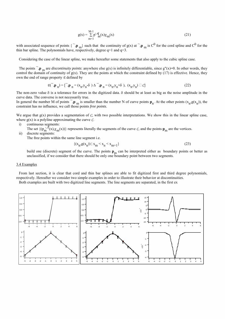
3.4 Examples

From last section, it is clear that cord and thin bar splines are able to fit digitized first and third degree polynomials, respectively. Hereafter we consider two simple examples in order to illustrate their behavior at discontinuities.

Both examples are built with two digitized line segments. The line segments are separated, in the first ex

-5

-4

-3

-2

-1

0

-5 -4 -3 -2 -1 0 1 2 3 4 5

-1.0

-0.5

0.0

0.5

1.0

-6 -4 -2 0 2 4 6

-5

-4

-3

-2

-1

0

-5 -4 -3 -2 -1 0 1 2 3 4 5

-4

-3

-2

-1

0

x10

-3

-5 -4 -3 -2 -1 0 1 2 3 4 5

15

10

5

0

-5

-10

-15

x10

-3

-6 -4 -2 0 2 4 6

-1.0

-0.5

0.0

0.5

1.0

-6 -4 -2 0 2 4 6

Fig.1. Curve segmentation by linear spline approximation

top: step discontinuity bottom: roof discontinuity

Fig.2. Curve segmentation by cubic spline approximation top: step discontinuity, bottom: roof discontinuity left: cubic spline, right: cubic spline second derivative

ample, by a C0 (step or jump) discontinuity, in the second, by a C1(roof or crease) discontinuity. In the corresponding figures, fig. 1 for the linear spline and fig. 2 for the cubic spline, the intervals [yn-δ, yn+δ] are represented with error bars, the endpoints and discontinuity points with a diamond marker. For the cubic spline we have represented its second derivative, which is a piecewise linear function. Note that g"(x), which has a peak at the discontinuity, goes through an intermediate state before reaching the value zero. In the simple example given here the linear spline performs well since it produces two discontinuity points in the case of the step and one for the roof discontinuity. The cubic spline produces however disturbing discontinuity points.

4. SPLINE FUNCTIONALS TO SEGMENT 2.5D DIGITIZED SURFACES 4.1 Extension of one-dimensional splines 4.1.1 Two-dimensional spline functionals The two-dimensional spline functional of order one is the expression

⊆f ⊆2,1 = ⌡⌠D 2

(f2x+f2y)dxdy (24)

where fx and fy are the first order partial derivatives of f and D2 a connected domain of IR2. ⊆f ⊆2,1 .is called harmonic spline or, because of its physical interpretation, membrane (rubber sheet) spline. The second order spline

⊆f ⊆2,2 = ⌡⌠D 2

(f2xx+2f2xy+f2yy)dxdy (25)

is called biharmonic spline or thin plate spline. Note that fxx, fxy and fyy are the second order partial derivatives of f. 4.1.2 Variational problem

The variational problem that led to the segmentation of a 1.5D curve is formulated for the case of a graph surface. We first introduce some definitions and notations. 4.1.2.1 Definitions Given the Cartesian coordinate system (O,ex,ey,ez) in IR3, we consider the 2.5D digitized surface S defined by the set {pn} = {(x0,y0,z0),(x1,y1,z1), …,(xn,yn,zn), …, (xN-1,yN-1,zN-1)} (26)

We define DS as any simple connected domain of IR2 containing all the points (xn,yn):

(xn,yn) ∈ DS, ∀n ∈ {0,1,…,N-1} (27)

we write Γ(DS) for the boundary of DS

The standard notations ∂f∂n and

∂f∂s are used for, respectively, the derivative across and along Γ(DS)

4.1.2.1 Variational problem The elements of the variational problem we pose are:

i) functional ⊆f ⊆2,p , as defined by (24) for the membrane spline and by (25) for the thin plate spline ii) constraints

|zn -f(xn,yn)| ≤ δ , ∀n {0,1,…,N-1} and δ > 0 (28)

iii) natural boundary conditions for the harmonic spline

∂f∂n = 0, ∀(x,y) Γ(DS) (29)

and for the biharmonic spline7,9

-∆f + ∂2f∂s2 = 0, ∀(x,y) Γ(DS) (30)

∂∂n ∆f +

∂∂s

∂2f∂s∂n = 0, ∀(x,y) Γ(DS) (31)

where ∆ denotes the Laplacian operator. Note that the Euler equations corresponding to the functionals ⊆f ⊆2,1 and ⊆f ⊆2,2 are ∆f = 0 (32) and

∆2f = 0 (33) respectively.

The physical interpretation of g(x) is the equilibrium position of a membrane or, respectively, a thin plate constrained in its

z-position within the interval [zn-δ,zn+δ]. 4.1.2.3 Discontinuities and segments

As in the 1.5D case, the solution g(x) to the variational problem gives rise to discontinuity points {~,p m}. However the way leading to segmentation is no more straightforward. In fact, in order to get 2D segments, discontinuity points have to build contour lines and this is not necessarily the case. 4.1.3 The way to segmentation

Hereafter we present our heuristic approach that has revealed itself efficient in practice in order to build contour lines form discontinuity points and segment range images. The basic idea is to perform a dilatation on the discontinuity points, however in an unconventional way. 4.1.3.1 Short review on second-order derivatives

We briefly recall that the directional second-order derivative of a function of two variables has two extreme values. They are independent of the coordinate system. We call these values principal second-order derivatives and write f " m and f " M. The Laplacian is the sum of the principal second-order derivatives. ∆f = f " m + f " M (34)

The product of f " m and f " M satisfies following equation

f " m·f " M = fxx fyy -f2 xy (35)

As short notation for this product, we use fΠ = f " m·f " M (36)

We note further that if the Laplacian is equal to zero (32), then f " m and f " M have the same absolute value. We hence write

fΠ = -(f " M)2 (37)

4.1.3.2 Heuristic

In the harmonic spline case, the Laplacian, i.e. the sum of principal second derivatives is equal to zero, except at discontinuity points ~,p m. There is however no constraint over the product of the two principal second derivatives. In our approach, we link discontinuity points by appending to the set {~,p m} those points pn which show a high H1(pn) = -fΠ (38)

value. By analogy, we have chosen the function H2 for the biharmonic spline as (∆f)Π i.e.

H2(pn) = ∂2

∂x2 ∆f · ∂2

∂y2 ∆f - (∂2

∂x∂y ∆f)2 (39)

4.2 Algorithm We summarize the method with the following algorithm:

i) solve the variational problem posed in section 4.1.3 In fact a discrete version of the variational problem will be solved. Since in our case the general graph-surface defined

in section 4.1.2 is a Cartesian range image, the points pn satisfy the equation (3). It is straightforward to use the image grid for the discretization.

ii) find the discontinuity points {~,p m}. In practice we take the end range points ~,p n, i.e. those for which E(~,p n) is true iii) create the boundaries by expanding the set {~,p m} with the points satisfying

Hp(pn) < -ρ2 (40)

where p is the order of the spline and -ρ2 is an arbitrary negative threshold value. 4.3 Computation

The computation-intensive part of the algorithm presented in last section is the resolution of the variational problem. Much work has been invested since years in order to efficiently solve variational problems involving harmonic and biharmonic spline functionals. There are basically two approaches for fast computation. In the first one, the computation is performed on an analog electrical network16,23. The second one applies iterative methods implemented on massively parallel computers14. Since the classical Jacobi iteration algorithm converges too slowly in order to have any practical interest, more performant algorithms have been developed. Conjugate gradient descent and adaptive Chebychev acceleration method have been investigated8,19 as well as multigrid10,22 and hierarchical basis functions method.20 In our current approach, we have applied the Jacobi method with a relaxation factor ω<1 for the membrane spline and the SSOR (Symmetric Successive Overrelaxation)12 for the thin plate spline. Hence, for the harmonic spline, starting with

vij(0) =

zij∆d (41)

the relaxation process repeats the step

vij(t+1/2) = vij

(t) + ω4 ∆vij

(t) (42)

vij(t+1) = min⎝

⎛⎠⎞max⎝

⎛⎠⎞vij

(0)-δ∆d, vij

(t+1/2) ,vij(0)+

δ∆d (43)

until fulfilling of the stopping condition max

{ij| E(pij)} |∆vij

(t) | < ε (44)

where ε is a small positive real value. Note that since the discrete form of the Laplacian is

∆vij = v(i-1)j + vi(j-1) + v(i+1)j + vi(j+1) - 4vij (45)

equation (42) can be rewritten as

vij(t+1/2) = (1-ω)vij

(t) + ω4 (v(i-1)j

(t) + vi(j-1)(t) + v(i+1)j

(t) + vi(j+1)(t)) (46)

and corresponds to a simple neighborhood operation. Without giving here any proof, we state that for (ω<1) the algorithm converges and that the test for the iterations to stop (44) can be replaced by the simpler condition

max ∀ij

|vij(t+1)

-vij(t)

| < ω4 ε (47)

In the case of the biharmonic spline, we proceed in a similar way.

5. EXPERIMENTS AND RESULTS 5.1 Test data

The segmentation method has been tested on numerous synthetic as well as sensed 256∞256 range images. The sensed images stem from the NRCC set of range images.18 Most of them contain manufactured objects with planar and curved surfaces. The synthetic images represent objects with planar faces, separated by jump and roof discontinuities. The geometric signal has been corrupted by Gaussian distributed random noise with predetermined σn. 5.2 Comments on the results

Both membrane spline and thin plate spline have been applied to images of objects with planar and curved surfaces separated by step and crease discontinuities.

The results of the different steps of the algorithm described in section 4.2 are represented in fig.3 and fig.4 for, respectively,

the harmonic and biharmonic spline. The grey-scale coded range image is at top left. Black is reserved for NIL values. The "end of range image" at top right represents in dark, points having a NIL value, and end of range points (those for which E(~,p ij) is true). The white regions represent free points. The bottom left image represents the value of H1 and H2 in fig.3 and fig.4, respectively. The positive values of H1 and H2 have been truncated the other have been grey coded using a logarithmic scale. White regions correspond to positive values of H1 and H2. They arise where ∆f and ∆2f, respectively are not equal to zero. This is either at discontinuity points or where the iterative process has not sufficiently converged. The segmentation result is represented in the bottom right image by coloring the regions with four different colors (in the figures, intensity values).

Fig.5 and fig.6 compare the results obtained with the membrane spline to those obtained with the thin plate spline. The

biharmonic spline is able to approximate planar as well as curved surfaces. The harmonic spline is only suited for planar surfaces. As we have already observed in the 1.5D case, the second-order spline generates many discontinuity points where discontinuities are present in the input data.

Fig.7 and fig.8 are two examples of a scene with manufactured objects and, respectively, natural objects in which the thin

plate spline delivers a satisfying segmentation result. 5.3 Discussion

Fig.9 compares the segmentation result of the membrane spline for two different noise sigma values. Obviously, the segmentation becomes critical with increasing noise. The step constraint we have introduced allows to smooth data within the surface patches. However, this is not the case at their boundaries. The constraints at discontinuity points disable the smoothing of the surface in the tangential direction to the discontinuity.

6. CONCLUSION

In the present paper, we have shown how controlled-continuity splines can be used for range image segmentation purposes. From a scientific point of view, the interest of the method lies in its physical analogy. Its parallel nature and the existence of corresponding digital and analog hardware for its computation establish its technical attractiveness. The method delivers membrane or thin plate spline approximation of the surface together with discontinuity points. The latter do not necessarily build a contour line, but a heuristic method has been given that performs the grouping of discontinuity points into lines. A series of experiments was also presented that show the effectiveness of our method to segment planar and curved surfaces found in range images. We think therefore that the controlled-continuity spline approximation of range images can be con-sidered as a basic segmentation step useful for the further fitting of geometric primitives.

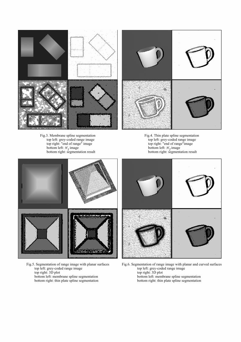
Fig.3. Membrane spline segmentation top left: grey-coded range image top right: "end of range" image bottom left: H1 image bottom right: segmentation result

Fig.4. Thin plate spline segmentation top left: grey-coded range image top right: "end of range"image bottom left: H2 image bottom right: segmentation result

Fig.5. Segmentation of range image with planar surfaces top left: grey-coded range image top right: 3D plot bottom left: membrane spline segmentation bottom right: thin plate spline segmentation

Fig.6. Segmentation of range image with planar and curved surfaces top left: grey-coded range image top right: 3D plot bottom left: membrane spline segmentation bottom right: thin plate spline segmentation

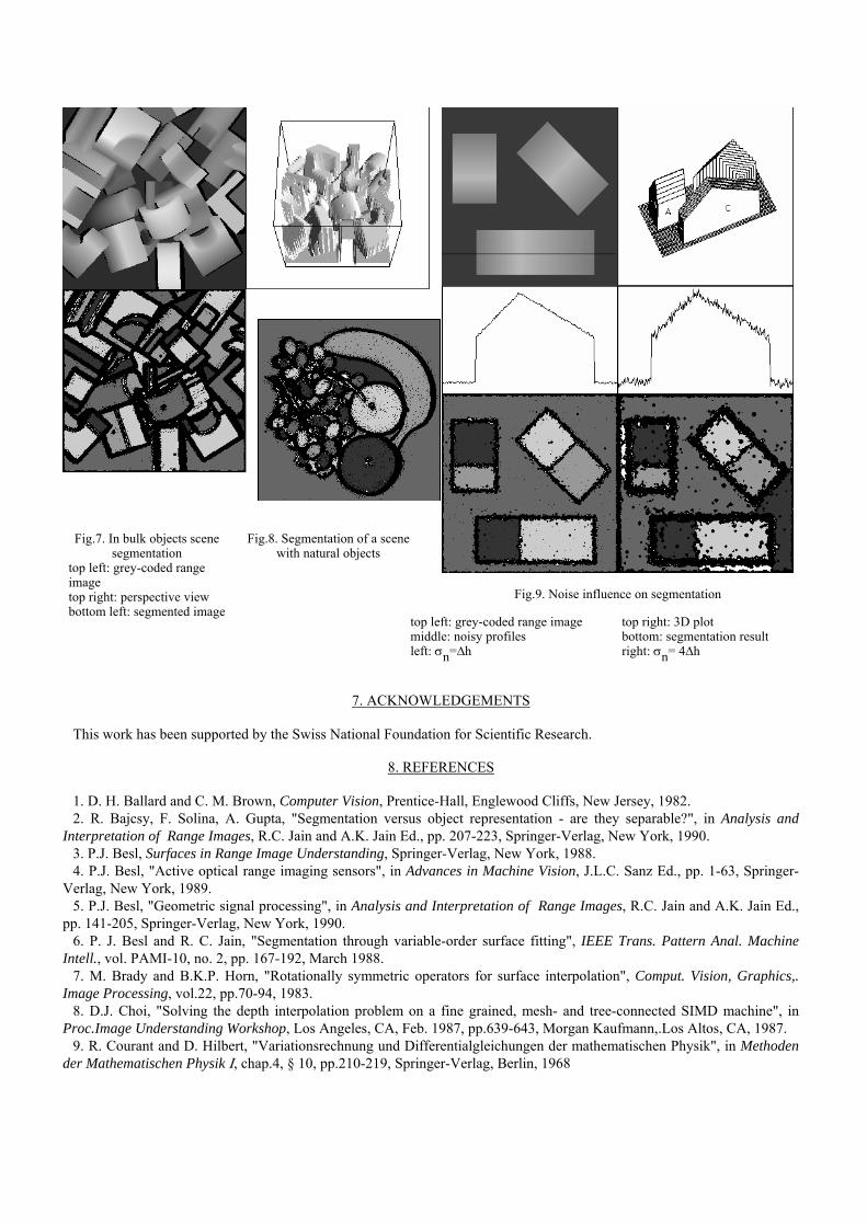
Fig.7. In bulk objects scene segmentation

top left: grey-coded range image top right: perspective view bottom left: segmented image

Fig.8. Segmentation of a scene with natural objects

Fig.9. Noise influence on segmentation

top left: grey-coded range image top right: 3D plot middle: noisy profiles bottom: segmentation result left: σn=∆h right: σn= 4∆h

7. ACKNOWLEDGEMENTS

This work has been supported by the Swiss National Foundation for Scientific Research.

8. REFERENCES

1. D. H. Ballard and C. M. Brown, Computer Vision, Prentice-Hall, Englewood Cliffs, New Jersey, 1982. 2. R. Bajcsy, F. Solina, A. Gupta, "Segmentation versus object representation - are they separable?", in Analysis and

Interpretation of Range Images, R.C. Jain and A.K. Jain Ed., pp. 207-223, Springer-Verlag, New York, 1990. 3. P.J. Besl, Surfaces in Range Image Understanding, Springer-Verlag, New York, 1988. 4. P.J. Besl, "Active optical range imaging sensors", in Advances in Machine Vision, J.L.C. Sanz Ed., pp. 1-63, Springer-

Verlag, New York, 1989. 5. P.J. Besl, "Geometric signal processing", in Analysis and Interpretation of Range Images, R.C. Jain and A.K. Jain Ed.,

pp. 141-205, Springer-Verlag, New York, 1990. 6. P. J. Besl and R. C. Jain, "Segmentation through variable-order surface fitting", IEEE Trans. Pattern Anal. Machine

Intell., vol. PAMI-10, no. 2, pp. 167-192, March 1988. 7. M. Brady and B.K.P. Horn, "Rotationally symmetric operators for surface interpolation", Comput. Vision, Graphics,.

Image Processing, vol.22, pp.70-94, 1983. 8. D.J. Choi, "Solving the depth interpolation problem on a fine grained, mesh- and tree-connected SIMD machine", in

Proc.Image Understanding Workshop, Los Angeles, CA, Feb. 1987, pp.639-643, Morgan Kaufmann,.Los Altos, CA, 1987. 9. R. Courant and D. Hilbert, "Variationsrechnung und Differentialgleichungen der mathematischen Physik", in Methoden

der Mathematischen Physik Ι, chap.4, § 10, pp.210-219, Springer-Verlag, Berlin, 1968

10. F. Glazer, "Multilevel relaxation in low-level computer vision", in Multiresolution Image Processing and Analysis, A. Rosenfeld Ed., pp. 312-330, Springer-Verlag, Berlin, 1984.

11. W.E.L. Grimson, "An implementation of a computational theory of visual surface interpolation", Comput. Vision, Graphics,. Image Processing, vol.22, pp.39-694, 1983.

12. L.A. Hageman and D.M. Young, Applied Iterative Methods, Academic Press, Orlando, 1981. 13. J.G. Harris, "A new approach to surface reconstruction: the coupled depth/slope model", in Proc. IEEE 1st Int.. Conf.

on Comput. Vision, pp. 277-283, London, England,June 8-11, 1987. 14. R.W. Hockney and C.R. Jesshope, Parallel Computers 2: architecture, programming and algorithms, Adam Hilger,

Bristol, England, 1988. 15. R. Jain and A.K. Jain, "Report: 1988 NSF Range Image Understanding Workshop", in Analysis and Interpretation of

Range Images, R.C. Jain and A.K. Jain Ed., pp. 1-31, Springer-Verlag, New York, 1990. 16. S.C. Liu and J.G. Harris, "Second-order smoothing networks in early vision", in Proc. 6th Scandinavian Conf. on

Image Analysis, vol. 2, pp. 1108-1117, Oulu, Finland,June 19-22, 1989. 17. G. Maître, H. Hügli, F. Tièche and J. P. Amann, "Range image segmentation based on function approximation", in

Proc.SPIE, vol. 1395, A. Gruen and E. Baltsavias Ed., pp.275-282, ISPRS CommissionV Symposium "Close-Range Photogrammetry Meets Machine Vision", 3-7 September 1990, Zurich, Switzerland.

18. M. Rioux and L. Cournoyer, "The NRCC three-dimensional image data files", Tech. rep. CNRC-29077, Division Elec. Eng., National Research Council Canada, Ottawa, Canada, June 1988.

19. T. Simchony, R. Chellappa and Z. Lichtenstein, "Pyramid implementation of optimal step conjugate search algorithms for some computer vision problems", in Proc. Second Int. Conf. Computer Vision (ICCV'88), Tampa, FL, Dec. 1988, pp.580-590, IEEE Computer Society Pess,.Washington, DC, 1988.

20. R. Szeliski, "Fast surface interpolation using hierarchical basis functions", IEEE Trans. Pattern Anal. Machine Intell., vol. PAMI-12, no.6, pp.513-528, June 1990.

21. D. Terzopoulos, "Multivel computational processes for visual surface reconstruction", Comput. Vision, Graphics,. Image Processing, vol.24, pp.52-96, 1983.

22. D. Terzopoulos, "Regularization of inverse visual problems involving discontinuities", IEEE Trans. Pattern Anal. Machine Intell., vol. PAMI-8, no.4, pp.413-424, July 1986.

23. D. Terzopoulos, "The computation of visible-surface representations", IEEE Trans. Pattern Anal. Machine Intell., vol. PAMI-10, no.4, pp.417-438, July 1988.