Chapter 1 Limits and Continuity

Chapter 1

Limits and Continuity

1.1 Limits

The limits is the fundamental notion of calculus. This underlying concept is the threadthat binds together virtually all of the calculus you are about to study.

In this section, we develop the notion of limit using some common language and illustratethe idea with some simple examples.

As a start, consider the function

f(x) =x2 − 1

x− 1and g(x) =

x2 − 2

x− 1

Notice that both functions are undefined at x = 1. But we can examine their behavior forx close to 1, as in the following table.

x f(x) =x2 − 1

x− 1g(x) =

x2 − 2

x− 10.9 1.9 11.90.99 1.99 101.990.999 1.999 1, 001.9990.9999 1.9999 10, 001.99990.99999 1.99999 100, 001.999990.999999 1.999999 10, 000, 001.999999

Notice that as you move down the first column of the table, the x-values get closer to 1,but all less than 1. We use the notation x → 1− to indicate that x approaches 1 from

the left side. Notice that the table suggest that as x gets closer and closer to 1 (withx < 1), f(x) is getting closer and closer to 2. In view of this, we say that the limit of f(x)as x approaches 1 from the left is 2, written

limx→1−

f(x) = 2.

On the other hand, the table indicate that as x gets closer and closer to 1 (with x > 1),g(x) increases without bound. In this case, g(x) is said to increase without bound as x

1

MA111 (Section 750001): Prepared by Dr.Archara Pacheenburawana 2

approaches 1 from the left, written

limx→1−

g(x) = +∞

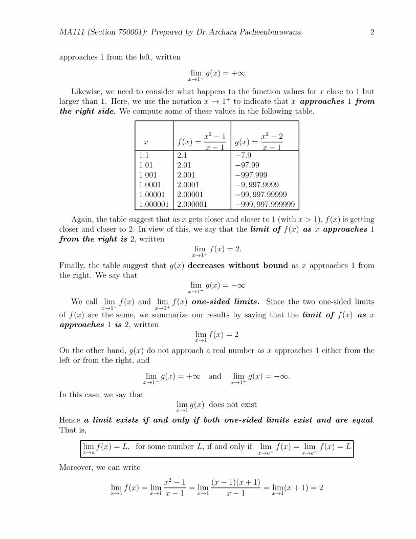
Likewise, we need to consider what happens to the function values for x close to 1 butlarger than 1. Here, we use the notation x → 1+ to indicate that x approaches 1 from

the right side. We compute some of these values in the following table.

x f(x) =x2 − 1

x− 1g(x) =

x2 − 2

x− 11.1 2.1 −7.91.01 2.01 −97.991.001 2.001 −997.9991.0001 2.0001 −9, 997.99991.00001 2.00001 −99, 997.999991.000001 2.000001 −999, 997.999999

Again, the table suggest that as x gets closer and closer to 1 (with x > 1), f(x) is gettingcloser and closer to 2. In view of this, we say that the limit of f(x) as x approaches 1from the right is 2, written

limx→1+

f(x) = 2.

Finally, the table suggest that g(x) decreases without bound as x approaches 1 fromthe right. We say that

limx→1+

g(x) = −∞

We call limx→1−

f(x) and limx→1+

f(x) one-sided limits. Since the two one-sided limits

of f(x) are the same, we summarize our results by saying that the limit of f(x) as xapproaches 1 is 2, written

limx→1

f(x) = 2

On the other hand, g(x) do not approach a real number as x approaches 1 either from theleft or from the right, and

limx→1−

g(x) = +∞ and limx→1+

g(x) = −∞.

In this case, we say thatlimx→1

g(x) does not exist

Hence a limit exists if and only if both one-sided limits exist and are equal.That is,

limx→a

f(x) = L, for some number L, if and only if limx→a−

f(x) = limx→a+

f(x) = L

Moreover, we can write

limx→1

f(x) = limx→1

x2 − 1

x− 1= lim

x→1

(x− 1)(x+ 1)

x− 1= lim

x→1(x+ 1) = 2


where we can cancel the factors (x − 1) since in the limit as x → 1, x is close to 1, butx 6= 1, so that x− 1 6= 0.

Example 1.1 Determine whether or not limx→0

1

xexists.

Solution We first graph y =1

xand compute some function values for x close to 0.

−3 3

10

−10

x

y

y =1

x

x 1/x±0.1 ±10±0.01 ±100±0.001 ±1000±0.0001 ±10, 000±0.00001 ±100, 000

Notice that, as x → 0+,1

xincreases without bound. Thus,

limx→0+

1

x= +∞.

Likewise, we can say that

limx→0−

1

x= −∞.

Therefore,

limx→0

1

xdoes not exist. ♣

Example 1.2 Evaluate limx→0

sin x

x.

Solution We graph f(x) =sin x

xand compute some function values.

x

y

y =sinx

x

1

0 1 2 3−1−2−3

x (sin x)/x

±0.1 0.998334±0.01 0.999983±0.001 0.99999983±0.0001 0.9999999983±0.00001 0.999999999983

The graph and the tables of value lead us to

limx→0+

sin x

x= 1 and lim

x→0−

sin x

x= 1


Thus,

limx→0

sin x

x= 1. ♣

Example 1.3

x

y

b bc

b

bc

0 1 2 3 4 5 6 7 8−1−2−3−4

0

1

2

3

4

5

6

7

−1

−2

For the function whose graph is given, state the value of the given quantity, if it does notexist, explain why.

(a) limx→2−

f(x) (b) limx→2+

f(x)

(c) limx→2

f(x) (d) limx→−1−

f(x)

(e) limx→−1+

f(x) (f) limx→−1

f(x)

Solution . . . . . . . . .

1.2 Computing Limits

In this section, we present some basic rules for dealing with common limit problem.

Theorem 1.1 For any constant c and any real number a,

limx→a

c = c.

Theorem 1.2 For any real number a,

limx→a

x = a.

Theorem 1.3 Suppose that limx→a

f(x) and limx→a

g(x) both exist and let c be any constant. The

following then apply:

1. limx→a

[

cf(x)]

= c limx→a

f(x)


2. limx→a

[

f(x)± g(x)]

= limx→a

f(x)± limx→a

g(x)

3. limx→a

[

f(x) · g(x)]

= limx→a

f(x) · limx→a

g(x)

4. limx→a

f(x)

g(x)=

limx→a

f(x)

limx→a

g(x)

(

if limx→a

g(x) 6= 0)

Corollary 1.1 Suppose that limx→a

f(x) exists. Then,

limx→a

[

f(x)]2

=[

limx→a

f(x)]2

.

Likewise, for any positive integer n,

limx→a

[

f(x)]n

=[

limx→a

f(x)]n

.

Corollary 1.2 For any integer n > 0 and for real number a,

limx→a

xn = an.

Example 1.4 Apply the rules of limits to evaluate the following.

(a) limx→4

(5x2 + 3x− 2) (b) limx→2

x3 + 2x− 5

x2 − 3

Solution . . . . . . . . .

Theorem 1.4 For any polynomial

p(x) = cnxn + cn−1x

n−1 + · · ·+ c1x+ c0

and any real number a,

limx→a

p(x) = cnan + cn−1a

n−1 + · · ·+ c1a+ c0 = p(a)

Example 1.5 Evaluate limx→−3

x2 − 14x− 51

x2 − 4x− 21. (Exam)

Solution . . . . . . . . .


(

4x2

x− 2− 8x

x− 2

)

.

Solution . . . . . . . . .

Example 1.7 Evaluate limx→2−

|x− 2|x3 + x2 − 6x

.

Solution . . . . . . . . .



x2/3 − 41/3

x− 2.

Solution . . . . . . . . .

Theorem 1.5 Suppose that limx→a

f(x) = L and n is any positive integer. Then,

limx→a

n

√

f(x) = n

√

limx→a

f(x) =n

√L,

where for n even, we assume that L > 0.


3

√

2x

1− 7x.

Solution . . . . . . . . .


√x+ 1− 2

x3 − 27. (Exam)

Solution . . . . . . . . .


x2 − 4x√2x2 − 7x− 2

. (Exam)

Solution . . . . . . . . .


2− 3√x+ 6

x− 2.

Solution . . . . . . . . .

For functions that are defined piecewise, a two-sided limit at a point where the formulafor the function changes is best obtained by first finding the one-sided limits at the point.


f(x), where f is defined by

f(x) =

x2 − 5x+ 6

|x− 2| for x ≤ 2

2x− 1

x+ 1for x > 2

Solution . . . . . . . . .

Theorem 1.6 (Squeeze Theorem)Suppose that

g(x) ≤ f(x) ≤ h(x)

for all x in some interval (c, d), except possibly at the point a ∈ (c, d) and that

limx→a

g(x) = limx→a

h(x) = L

for some number L. Then, it follows that

limx→a

f(x) = L.


0 a x

L

y

g

f

h

Remark. Squeeze Theorem also applied to one-sided limits.


f(x) if 8 + 2x− x2 ≤ f(x) ≤ 4x+ 5 for all x ∈ R.

Solution . . . . . . . . .

Example 1.15 Determine the value of

limx→0

[√x2 + x sin

( π

2x

)]

.

Solution . . . . . . . . .

1.3 Limits at Infinity

Let’s begin by investigating the behavior of the function f defined by

f(x) =x2 − 1

x2 + 1

as x becomes large.

x

yy = 1

x (sin x)/x

±0 −1±1 0±2 0.600000±3 0.800000±4 0.882353±5 0.923077±10 0.980198±50 0.999200±100 0.999800±1000 0.999998

As x grows larger and larger we can see from the graph and the table of values that thevalues of f(x) get closer and closer to 1. That is,

limx→∞

x2 − 1

x2 + 1= 1.


In general, we use the notationlimx→∞

f(x) = L

indicates that the values of f(x) becomes closer and closer to L as x becomes larger andlarger.

Definition 1.1 Let f be a function defined on some interval (a,∞). Then

limx→∞

f(x) = L

mean that the value of f(x) can be made arbitrarily close to L by taking x sufficiently large.

Referring back to the above Figure, we see that for numerically large negative values ofx, the values of f(x) are close to 1, that is,

limx→−∞

x2 − 1

x2 + 1= 1.

The general definition is as follows.

Definition 1.2 Let f be a function defined on some interval (−∞, a). Then

limx→−∞

f(x) = L

mean that the value of f(x) can be made arbitrarily close to L by taking x sufficiently largenegative.

Definition 1.3 The line y = L is called a horizontal asymptote of the curve y = f(x)if either

limx→∞

f(x) = L or limx→−∞

f(x) = L

For instance, the curve illustrated in Figure above has the line y = 1 as a horizontalasymptote because

limx→∞

x2 − 1

x2 + 1= 1.

Theorem 1.7 For any rational number t > 0,

limx→±∞

1

xt= 0

where for the case where x → −∞, we assume that t =p

qwhere q is odd.

Theorem 1.8 For a polynomial of degree n > 0,

pn(x) = anxn + an−1x

n−1 + · · ·+ a1x+ a0,

we have

limx→∞

pn(x) =

{

∞, if an > 0−∞, if an < 0


Example 1.16 Evaluate limx→∞

x3 − x2 + 5x− 3

2x4 − 3x+ 5.

Solution . . . . . . . . .


3x2 − 5x+ 2√4x4 + 2x+ 3

. (Exam)

Solution . . . . . . . . .


(√25x2 + 4x− 5x

)

.

Solution . . . . . . . . .

Example 1.19 Evaluate limx→−∞

3x− 4x2

√x6 − 1 + 5x2

.

Solution . . . . . . . . .

1.4 Limit of Trigonometric Functions

Lemma 1.1limθ→0

sin θ = 0

Lemma 1.2

limθ→0

sin θ

θ= 1

Corollary 1.3 For any real number k 6= 0,

limθ→0

sin kθ

θ= k


sin 2x+ sin 3x

x.

Solution . . . . . . . . .


1− cos 2x

x2.

Solution . . . . . . . . .


3x2 tan2 x

4x sec x.

Solution . . . . . . . . .


tan 3x

tan 5x.

Solution . . . . . . . . .


x

y

ax

y

b

ax

y

a

1.5 Continuity

It is helpful for us to first try to see what it is about the function whose graphs are shownbelow that makes them discontinuous at the point x = a.

This suggests the following definition of continuity at a point.

Definition 1.4 A function f is continuous at x = a when

(i) f(a) is defined,

(ii) limx→a

f(x) exists and

(iii) limx→a

f(x) = f(a).

Otherwise, f is said to be discontinuous at x = a.

Example 1.24 From the graph of f , state the numbers at which f is discontinuous andexplain why.

x

y

b

0 1 3 5

Solution . . . . . . . . .

Example 1.25 Where are each of the following functions discontinuous?

(a) f(x) =2x2 − 5x− 3

x− 3

(b) g(x) =

2x2 − 5x− 3

x− 3if x 6= 3

6 if x = 3

Solution . . . . . . . . .


Example 1.26 For what value of the constant k is the function (Exam)

f(x) =

{

x2 − k2 if x < 4kx+ 20 if x ≥ 4

continuous on (−∞,∞).

Solution . . . . . . . . .

Example 1.27 Let (Exam)

f(x) =

(x− 2)2

x2 − 4+ 2k if x > 2

h if x = 2

2x+ k if x < 2

Find the values h and k so that f is continuous at x = 2.

Solution . . . . . . . . .

Definition 1.5 A function f is continuous from the right at a number a if

limx→a+

f(x) = f(a)

and f is continuous from the left at a if

limx→a−

f(x) = f(a).

Definition 1.6 A function f is is said to continuous on a closed interval [a, b] if thefollowing conditions are satisfied:

1. f is continuous on (a, b).

2. f is continuous from the right at a.

3. f is continuous from the left at b.

Example 1.28 Show that the function

f(x) = x√16− x2

is continuous on the interval [−4, 4].

Solution . . . . . . . . .

Theorem 1.9 If f and g are continuous at a and c is a constant, then the followingfunctions are also continuous at a:

(a) f + g (b) f − g (c) cf

(d) f · g (e)f

gif g(a) 6= 0


The following types of functions are continuous at every number in their domains:

• polynomials

• rational functions

• root functions

• trigonometric functions

• inverse trigonometric functions

• exponential functions

• logarithmic functions

Example 1.29 Where is the function

h(x) =x4 − 3x+ 1

x2 − x− 6

continuous?

Solution . . . . . . . . .

Theorem 1.10 If limx→a

g(x) = L and f is continuous at L, then

limx→a

f(

g(x))

= f(

limx→a

g(x))

= f(L)

Corollary 1.4 If g is continuous at a and f is continuous at g(a), then the compositefunction f ◦ g given by (f ◦ g)(x) = f

(

g(x))

is continuous at a.

Theorem 1.11 (Intermediate Value Theorem)Suppose that f is continuous on the closed interval [a, b] and let N be any number betweenf(a) and f(b). Then there exists a number c ∈ (a, b) such that f(c) = N .

f(a)

N

f(b)

y

a c bx

y = f(x)

(a)

f(a)

N

f(b)

y

a c1 c2 c3 bx

y = f(x)

(b)

Note that the value N can be taken on once [as in part (a)] or more that once [as inpart (b)].


Corollary 1.5 Suppose that f is continuous on [a, b] and f(a) and f(b) have opposite signs.Then, there is at least one number c ∈ (a, b) for which f(c) = 0.

Example 1.30 Show that there is a root of the equation

4x3 − 6x2 + 3x− 2 = 0

between 1 and 2.

Solution . . . . . . . . .

Chapter 2

Differentiation

2.1 Tangent Lines and Rates of Change

2.1.1 Tangent Lines

If a curve C has equation y = f(x) and we want ti find the tangent to C at the pointP(

a, f(a))

, then we consider the nearby point Q(

x, f(x))

, where x 6= a, and compute theslope of the secant line PQ:

mPQ =f(x)− f(a)

x− a

y

x

P (a, f(a))

Q(x, f(x))

0 a x

x− a

f(x)− f(a)

Secant Line PQ

y

x0

bb

b

a x

Q

L

P

Q approach P

Then we let Q approach P along the curve C by letting x approach a. IfmPQ approachesa number m, then we define the tangent L to be the line through P with slope m.

Definition 2.1 The tangent line to the curve y = f(x) at the point P(

a, f(a))

is the linethrough P with slope

m = limx→a

f(x)− f(a)

x− a

provided that this limit exists.

14


Example 2.1 Find an equation of the tangent line to the hyperbola y =2

xat the point

(2, 1).

Solution . . . . . . . . .

There is another expression for the slope of a tangent line that is sometimes easier touse. Let h = x− a. Then x = a + h, so the slope of the secant line PQ is

mPQ =f(a+ h)− f(a)

h

Hence the expression for the slope of the tangent line in Definition 2.1 becomes

m = limh→0

f(a+ h)− f(a)

h

Example 2.2 Find an equation of the tangent line to f(x) =√x+ 2 at the point (−1, 1).

Solution . . . . . . . . .

2.1.2 Rate of Change

Velocities

Suppose an object moves along a straight line according to an equation of motion s = f(t),where s is the displacement of the object from the origin at time t. The function f thatdescribes the motion is called the position function of the object. In the time intervalfrom t = a to t = a + h the change in position is f(a+ h)− f(a)

(

see Figure 2.1 (a))

. Theaverage velocity over this time interval is

average velocity =displacement

time=

f(a+ h)− f(a)

h

which is the same as the slope of the secant line PQ in Figure 2.1 (b)

b

f(a+ h)− f(a)

position at

time t = a

position at

time t = a+ h

0s

f(a)

f(a+ h)

(a)

h

a a + h

P (a, f(a))

Q(

a+ h, f(a+ h))

s

t

s = f(t)

0

(b)

Figure 2.1:


Now suppose we compute the average velocities over shorter and shorter time intervals[a, a+ h]. In other words, we let h approach 0. We define the velocity of instantaneousvelocity v(a) at time t = a to be the limit of these average velocities:

v(a) = limh→0

f(a+ h)− f(a)

h

This mean that the velocity at time t = a is equal to the slope of the tangent line at P .

2.2 Derivatives

In previous section we define the tangent line to the curve with equation y = f(x) wherex = a to be

m = limh→0

f(a+ h)− f(a)

h.

We also saw that the velocity of an object with position function s = f(t) at time t = a is

v(a) = limh→0

f(a+ h)− f(a)

h

In fact, limits of the form

limh→0

f(a+ h)− f(a)

h

arise whenever we calculate a rate of change in any of the sciences or engineering, such asa rate of reaction in chemistry or a marginal cost in economics. Since this type of limitoccurs so widely, it is given a special name and notation.

Definition 2.2 The derivative of a function f(x) at x = a is defined by

f ′(a) = limh→0

f(a+ h)− f(a)

h

provided the limit exists. If the limit exists, we say that f is differentiable at x = a.

Example 2.3 Compute the derivative of f(x) = 2x3 + 3x− 1 at x = 1.

Solution . . . . . . . . .

Example 2.4 Find the derivative of f(x) = 2x3 + 3x − 1 at an unspecified value of x.Then, evaluate the derivative at x = 1, x = 2, and x = 3.

Solution . . . . . . . . .

This example leads us to the following definition.

Definition 2.3 The derivative of f(x) is the function f ′(x) given by

f ′(x) = limh→0

f(x+ h)− f(x)

h

provided the limit exists. The process of computing a derivative is called differentiation.


Example 2.5 Find the derivative of the function f(x) =2x− 3

5− xusing the definition of

derivative. (Exam)

Solution . . . . . . . . .

Other Notations

If we use the notation y = f(x) to indicate that the independent variable is x and thedependent variable is y, then some common alternative notations for the derivative are asfollows:

f ′(x) = y′ =dy

dx=

df

dx=

d

dxf(x) = Df(x) = Dxf(x)

The symbols D and d/dx are called differentiation operators.If we want to indicate the value of a derivative dy/dx at a specific number a, we use the

notation

f ′(a) =dy

dx

∣

∣

∣

∣

x=a

=d

dxf(x)

∣

∣

∣

∣

x=a

Definition 2.4 A function f is differentiable at a if f ′(a) exists. It is differentiable

on an open interval (a, b) or (a,∞) or (−∞, a) or (−∞,∞) if it is differentiable atevery number in the interval.

Theorem 2.1 If f is differentiable at a, then f is continuous at x = a.

2.3 Techniques of Differentiation

We have now computed numerous derivative using the limit definition. In this section wedevelop rules for finding derivatives without having to use the definition directly. Thesedifferentiation rules enable us to calculate the derivatives of polynomials, rational functions,algebraic functions, exponential and logarithmic functions, and trigonometric and inversetrigonometric functions.

The Power Rule

Theorem 2.2 For any constant c,

d

dx(c) = 0.

Theorem 2.3d

dx(x) = 1

Theorem 2.4 If n in any real number, then

d

dx(xn) = nxn−1


Example 2.6 Differentiate:

(a) f(x) = x15 (b) f(x) =1

x−3/4

(c) g(x) =3√x7 (d) h(x) = xπ

Solution . . . . . . . . .

General Derivative Rules

Theorem 2.5 If f and g are differentiable at x and c is any constant, then

(i)d

dx

[

cf(x)]

= cd

dxf(x)

(ii)d

dx

[

f(x) + g(x)]

=d

dxf(x) +

d

dxg(x)

(iii)d

dx

[

f(x)− g(x)]

=d

dxf(x)− d

dxg(x)

Example 2.7 Find the derivative of f(x) = 5x5/2 + 3x3/2 − 2√x+ 6x4 − 5.

Solution . . . . . . . . .

Example 2.8 Find the derivative of f(x) =5x3 − 2x+ 4

√x

x.

Solution . . . . . . . . .

Example 2.9 Find an equation of the tangent line to f(x) =x2 − 2x

2x3at x = 2.

Solution . . . . . . . . .

The Product and Quotient Rules

Theorem 2.6 The Product Rules

If f and g are both differentiable, then

d

dx

[

f(x)g(x)]

= f(x)d

dx

[

g(x)]

+ g(x)d

dx

[

f(x)]

Example 2.10 Use the product rule to find the derivative of

f(x) =(

3x4 − 4x+ 2)

(

x2 −√x+

3

x

)

.

Solution . . . . . . . . .

Example 2.11 Find f ′(x) if f(x) = x−7/8(x3 − 2x+ 1).

Solution . . . . . . . . .


Example 2.12 If f(x) =√x g(x), where g(4) = 2 and g′(4) = 3, find f ′(4).

Solution . . . . . . . . .

Theorem 2.7 The Quotient Rule

Suppose that f and g are differentiable at x and g(x) 6= 0. Then

d

dx

[

f(x)

g(x)

]

=g(x)

d

dx[f(x)]− f(x)

d

dx[g(x)]

[

g(x)]2 .

Example 2.13 Compute the derivative of f(x) =x2 + x+ 1

x3 + 4.

Solution . . . . . . . . .

Note. Don’t use the Quotient Rule every time you see the quotient. Sometimes it’s easierto rewrite a quotient first to put it in a form that is simpler for the purpose of differentiation.For instance, although it is possible to differentiate the function

F (x) =2x3 + x2 + 3

√x

x

using the Quotient Rule, it is much easier to perform the division first and then write thefunction as

F (x) = 2x2 + x+ 3x− 1

2

before differentiating.

2.4 Derivatives of Trigonometric Functions

We collect all the differentiation formulas for trigonometric functions in the following table.

d

dx(sin x) = cosx

d

dx(cosx) = − sin x

d

dx(tanx) = sec2 x

d

dx(cotx) = − csc2 x

d

dx(sec x) = sec x tanx

d

dx(csc x) = − csc x cotx

Example 2.14 Differentiate.

(a) f(x) = 3 tanx− 2 csc x

(b) g(x) = x4 sin x

(c) h(x) =sec x

1 + tanx

Solution . . . . . . . . .


2.5 The Chain Rule

Theorem 2.8 Chain RuleIf g is differentiable at x and f is differentiable at g(x), then

d

dx

[

f(

g(x))]

= f ′(g(x))

g′(x)

It is often to think of the chain rule in Leibniz notation. If y = f(u) and u = g(x), theny = f

(

g(x))

and the chain rule says that

dy

dx=

dy

du· dudx

Theorem 2.9 If n is any real number and u = g(x) is differentiable, then

d

dx(un) = nun−1du

dx

ord

dx

[

g(x)]n

= n[

g(x)]n−1 · g′(x)

Example 2.15 Differentiate y = (x3 + 5x− 2)5.

Solution . . . . . . . . .

Example 2.16 Find the derivative of g(x) =√tan x2 − sec 3x.

Solution . . . . . . . . .

Example 2.17 Let h(x) =

[

5x− 7

4− x

]2/3

. Find h′(x).

Solution . . . . . . . . .

Example 2.18 Find f ′(x) where f(x) =tan 2x

3√x3 − 2x

.

Solution . . . . . . . . .

Example 2.19 Differentiate y = sin2(x cosx+ ln 10).

Solution . . . . . . . . .

Example 2.20 Let y = 3u5 − 2u3 and u = 2x+ 3. Finddy

dx

∣

∣

∣

∣

x=1

.

Solution . . . . . . . . .


2.6 Implicit Differentiation

Compare the following two equations:

y =√x2 + 3 and x2 + y2 = 9.

The first equation defines y as a function of x explicitly, since for each x, the equationgives an explicit formula y = f(x) for finding the corresponding value of y. On the otherhand, the second equation does not define a function. However, we can solve for y and findat least two functions

(

y =√9− x2 and y = −

√9− x2

)

that are defined implicitly bythe equation x2 + y2 = 9.

To find the derivatives of functions defined implicitly, we can use the method of implicit

differentiation. This consists of differentiating both sides of the equation with respect to xand then solving the resulting equation for y′. In the examples and exercises of this sectionit is always assumed that the given equation determines y implicitly as a differentiablefunction of x so that the method of implicit differentiation can be applied.

Example 2.21 Find y′(x) for x3 + y2 − 3y = 5.

Solution . . . . . . . . .

Example 2.22 Find y′(x) if x2 cos y + sin 2y = xy. (Exam)

Solution . . . . . . . . .

Example 2.23 Find an equation of the tangent line to (Exam)

cos(xy2) = y2 + x

at the point (0, 1).

Solution . . . . . . . . .

2.7 Derivatives of Inverse Trigonometric Functions

We collect all the differentiation formulas for inverse trigonometric functions in the followingtable.

d

dx

(

sin−1 x)

=1√

1− x2when −1 < x < 1

d

dx(cos−1 x) =

−1√1− x2

when −1 < x < 1

d

dx(tan−1 x) =

1

1 + x2

d

dx(cot−1 x) =

−1

1 + x2

d

dx(sec−1 x) =

1

|x|√x2 − 1

when |x| > 1

d

dx(csc−1 x) =

−1

|x|√x2 − 1

when |x| > 1


Example 2.24 Differentiate

(a) y = cos−1(5x2) (b) y = (sec−1 x)2

(c) y = x tan−1√x

Solution . . . . . . . . .

2.8 Derivatives of Exponential and Logarithmic Func-

tion

2.8.1 Derivatives of Exponential Functions

Theorem 2.10 For any constant a > 0,

d

dx(ax) = ax ln a

The most commonly used base is the irrational number e.

Definition 2.5 e is the number such that

limh→0

eh − 1

h= 1.

Since ln e = 1, the derivative of f(x) = ex is simply:

d

dx(ex) = ex ln e = ex

We now have the following result.

Theorem 2.11d

dx(ex) = ex and

d

dx(e−x) = −e−x.

Example 2.25 Differentiate

(a) f(x) = 4x cos x (b) f(x) =x

ex

(c) f(x) = 2secx +1

3√etanx

Solution . . . . . . . . .


2.8.2 Derivatives of Logarithmic Functions

Theorem 2.12d

dx(loga x) =

1

x ln a(2.1)

If we put a = e in Formula (2.1), then the factor ln a on the right side becomes ln e = 1and we get the formula for the derivative of the natural logarithmic function loge x = ln x:

d

dx(ln x) =

1

x(2.2)

In general, if we combine Formula (2.2) with the Chain Rule, we get

d

dx(ln u) =

1

u

du

dxor

d

dx

[

ln g(x)]

=g′(x)

g(x)

Example 2.26 Differentiate:

(a) f(x) = log5(3 + tan x) (b) f(x) = ln[

cos(

ex2−sec x

)

]

(c) y = ln

(

x+ 1√x− 2

)

Solution . . . . . . . . .

Example 2.27 Find f ′(x) if f(x) = ln |x|.Solution . . . . . . . . .

Logarithmic Differentiation

The calculation of derivatives of complicated functions involving products, quotients, orpowers can often be simplified by taking logarithms. The method used in the followingexample is called logarithmic differentiation.

Example 2.28 Use logarithmic differentiation to find the derivative of (Exam)

y =x5(2x+ 5)4

3√

(1− 7x)2.

Solution . . . . . . . . .

Steps in Logarithmic Differentiation1. Take natural logarithms of both sides of an equation

y = f(x) and use the Laws of Logarithms to simplify.2. Differentiate implicitly with respect to x.3. Solve the resulting equation for y′.

Example 2.29 Differentiate y = (ln x)cos x by using logarithmic differentiation. (Exam)

Solution . . . . . . . . .

Example 2.30 Differentiate y = [ln(x+ 1)]sinx2

.

Solution . . . . . . . . .


2.9 Derivatives of Hyperbolic Functions

In this section we shall study certain combinations of ex and e−x, called hyperbolic func-

tions. These functions have numerous engineering applications and arise naturally in manymathematical problems.

Definition 2.6 The hyperbolic sine and hyperbolic cosine functions, denoted by sinhand cosh, respectively, are defined by

sinh x =ex − e−x

2and cosh x =

ex + e−x

2

The remaining hyperbolic functions, hyperbolic tangent, hyperbolic cotangent, hy-perbolic secant, and hyperbolic cosecant are defined in terms of sinh and cosh as follows.

tanh x =sinh x

cosh x=

ex − e−x

ex + e−x

coth x =cosh x

sinh x=

ex + e−x

ex − e−x

sech x =1

cosh x=

2

ex + e−x

csch x =1

sinh x=

2

ex − e−x

The graphs of these functions are shown in Figure below.

y = sinh xy = cosh x

−1

1

y = tanh x

y = cschx y = sechx

y = coth x


The hyperbolic functions satisfy a number of identities that are similar to well-knowntrigonometric identities. We list some of them here.

Hyperbolic Identities

sinh(−x) = − sinh x cosh(−x) = cosh x

tanh(−x) = − tanh x cosh2 x− sinh2 x = 1

1− tanh2 x = sech 2x coth2 x− 1 = csch 2x

cosh x+ sinh x = ex cosh x− sinh x = e−x

sinh 2x = 2 sinh x cosh x cosh 2x = cosh2 x+ sinh2 x

sinh(x± y) = sinh x cosh y ± cosh x sinh y

cosh(x± y) = cosh x cosh y ± sinh x sinh y

tanh(x± y) =tanh x± tanh y

1± tanh x tanh y

The derivatives of the hyperbolic functions are easily computed. For example,

d

dx(sinh x) =

d

dx

(

ex − e−x

2

)

=ex + e−x

2= cosh x.

We list the differentiation formulas for the hyperbolic functions as follows.

Derivatives of Hyperbolic Functions

d

dx(sinh x) = cosh x

d

dx(csch x) = −csch x coth x

d

dx(cosh x) = sinh x

d

dx(sech x) = −sech x tanh x

d

dx(tanhx) = sech 2x

d

dx(coth x) = −csch 2x

Note that any of these differentiation rules can be combined with the Chain Rule. Forinstance,

d

dx(cosh

√x) = sinh

√x · d

dx

√x =

sinh√x

2√x

.


(a) f(x) = tanh 4x+ sinh2 x

(b) g(x) = ln(sinh x)− sinh(cosh x)

(c) h(x) = sinh x tanhx+ exsech x

Solution . . . . . . . . .


Inverse Hyperbolic Functions

We can see from above Figures that sinh and tanh are one-to-one functions and so theyhave inverse functions denoted by sinh−1 and tanh−1. Moreover, the above Figure show thatcosh is not one-to-one, but when restricted to the domain [0,∞) it becomes one-to-one. Theinverse hyperbolic cosine function is defined as the inverse of this restricted function.

y = sinh−1 x ⇐⇒ sinh y = x

y = cosh−1 x ⇐⇒ cosh y = x if y ≥ 0

y = tanh−1 x ⇐⇒ tanh y = x

The remaining inverse hyperbolic functions are defined similarly. We can sketch the graphsof sinh−1 x, cosh−1 x, and tanh−1 x in Figures below.

y = sinh−1 xy = cosh−1 x

1 −1 1

y = tanh−1 x

Since the hyperbolic functions are defined in terms of exponential functions, it’s notsurprising to learn that the inverse hyperbolic functions can be expressed in terms of loga-rithms.

sinh−1 x = ln(x+√x2 + 1), x ∈ R csch −1x = ln

(

1

x+

√1 + x2

|x|

)

, x 6= 0

cosh−1 x = ln(x+√x2 − 1), x ≥ 1 sech −1x = ln

(

1 +√1− x2

x

)

, 0 < x ≤ 1

tanh−1 x = 12ln

(

1 + x

1− x

)

, |x| < 1 coth−1 x = 12ln

(

x+ 1

x− 1

)

, |x| > 1

The inverse hyperbolic functions are all differentiable because the hyperbolic functionsare differentiable. We list the differentiation formulas for the inverse hyperbolic functionsas follows.


Derivatives of Hyperbolic Functions

d

dx(sinh−1 x) =

1√1 + x2

d

dx(csch −1x) = − 1

|x|√x2 + 1

d

dx(cosh−1 x) =

1√x2 − 1

d

dx(sech −1x) = − 1

x√1− x2

d

dx(tanh−1 x) =

1

1− x2

d

dx(coth−1 x) =

1

1− x2


(a) f(x) = sech −1√1− x2 , x > 0

(b) g(x) = x tanh−1 x+ ln√1− x2

(c) h(x) = x2 sinh−1(2x) + tanh−1(sin x)

Solution . . . . . . . . .

2.10 Higher Derivatives

If the derivative f ′ of a function is itself differentiation, then the derivative of f ′ is denotedby f ′′ and is called the second derivative of f . As long as we have differentiability, wecan continue the process of differentiating derivatives to obtain third, fourth, fifth, and evenhigher derivatives of f . The successive derivatives of f are denoted by

f ′ The first derivative of f

f ′′ = (f ′)′ The second derivative of f

f ′′′ = (f ′′)′ The third derivative of f

f (4) = (f ′′′)′ The fourth derivative of f

f (5) =(

f (4))′

The fifth derivative of f

......

f (n) The n th derivative of f


Example 2.33 If f(x) = 5x3 − 2x2 + 1, then

f ′(x) =

f ′′(x) =

f ′′′(x) =

f (4)(x) =...

f (n)(x) =

Successive derivatives can also be denoted as follows:

f ′(x) =d

dx[f(x)]

f ′′(x) =d

dx

[

d

dx[f(x)]

]

=d2

dx2[f(x)]

f ′′′(x) =d

dx

[

d2

dx2[f(x)]

]

=d3

dx3[f(x)]

...

In general, we write

f (n)(x) =dn

dxn[f(x)]

Example 2.34 Let y = e√x. Find y′ and y′′.

Solution . . . . . . . . .

Example 2.35 Find y′′ if x2 − xy + y2 = 6.

Solution . . . . . . . . .

2.11 Linear Approximations and Differentials

2.11.1 Linear Approximations

We have seen that a curve lies very close to its tangent near the point of tangency. Thisobservation is the basis for a method of finding approximate values of functions.

The idea is that it might be easy to calculate a value f(a) of a function, but difficult(or even impossible) to compute nearby values of f . So we settle for the easily computedvalues of the linear function L whose graph is the tangent line to f at (a, f(a)).


x

y

b

(a, f(a))

y = f(x)

y = L(x)

0

In other words, we use the tangent line at (a, f(a)) as an approximation to the curvey = f(x) when x is near a. An equation of this tangent line is

y = f(a) + f ′(a)(x− a)

and the approximation

f(x) ≈ f(a) + f ′(a)(x− a) (2.3)

is called linear approximation or tangent line approximation of f at a. The linearfunction whose graph is this tangent line, that is,

L(x) = f(a) + f ′(a)(x− a)

is called the linearization of f at a.

Example 2.36 Find the linearization of (Exam)

f(x) = 3√x+ 1 at a = 7

and use it to approximate 3√8.024.

Solution . . . . . . . . .

Example 2.37 Use a linearization to approximate 3√8.02 and 3

√25.2.

Solution . . . . . . . . .

2.11.2 Differentials

The ideas behind linear approximations are sometimes formulated in the terminology andnotation of differentials. If y = f(x), where f is a differentiable function, then the differ-

ential dx is an independent variable; that is, dx can be given the value of any real number.The differential dy is then defined in terms of dx by the equation

dy = f ′(x)dx

So dy is a dependent variable; it depends on the values of x and dx.

Example 2.38 Find the differential of the function.

(a) y = x3 − 2x2 (b) y =√3x2 + x+ 1

(c) y = (x10 +√sin 2x)2 (d) y = (tan x+ 1)3

Solution . . . . . . . . .

Chapter 3

Applications of Differentiation

3.1 Related Rates

In this section we shall study related rates problems. In such problems one tries to findthe rate at which some quantity is changing by relating it to other quantities whose ratesof change are known.

The method for finding the solution of related rates problems consists of the following steps.

1. Read the problem carefully.

2. Draw a diagram if possible.

3. Introduce notation. Assign symbols to all quantities that are functions of time.

4. Express the given information and the required rate in terms of derivatives.

5. Write an equation the relates the various quantities of the problem.

6. Use the Chain Rule to differentiate both sides of the equation with respect to t.

7. Substitute the given information into the resulting equation and solve for the unknownrate.

The following examples are illustrations of the strategy.

Example 3.1 If the radius of a circle increases at a constant rate of 5 ft/s. How fast isthe area increasing when the radius of a circle is 15 ft?

Solution . . . . . . . . .

Example 3.2 Suppose a 6-ft tall person is 12 ft away from a 18-ft tall lamppost. If theperson is moving away from the lamppost at a rate of 2 ft/s, at what rate is the length ofthe shadow changing? (Exam)

Solution . . . . . . . . .

30


Example 3.3 A women standing on a cliff is watching a motor boat through a telescopeas the boat approaches the shoreline directly below her. If the telescope is 250 feet above thewater level and if the boat is approaching at 20 feet per second, at what rate is the angle ofthe telescope changing when the boat is 250 feet from shore?

Solution . . . . . . . . .

Example 3.4 A water tank has the shape of an inverted circular cone with base radius 2m and height 4 m. If water is being pumped into the tank at a rate of 2 m3/min, find therate at which the water level is rising when the water is 3 m deep.

Solution . . . . . . . . .

3.2 Indeterminate Forms and L’Hospital’s Rule

In general, if we have a limit of the form

limx→a

f(x)

g(x)

where both f(x) → 0 and g(x) → 0 as x → a, then this limit may or may not exist andis called an indeterminate form of type 0

0. In this section we introduce a systematic

method, known as l’Hospital’s Rule, for the evaluation of indeterminate forms.Moreover, if we have a limit of the form

limx→a

f(x)

g(x)

where both f(x) → ∞ (or −∞) and g(x) → ∞ (or −∞) as x → a, then this limit may ormay not exist and is called an indeterminate form of type ∞

∞ . L’Hospital’s Rule alsoapplies to this type of indeterminate form.

Theorem 3.1 (L’Hospital’s Rule)Suppose f and g are differentiable and g′(x) 6= 0 near a (except possible at a). Suppose that

limx→a

f(x) = 0 and limx→a

g(x) = 0

or thatlimx→a

f(x) = ±∞ and limx→a

g(x) = ±∞(

In other words, we have an indeterminate form of type 00or ∞

∞ .)

Then

limx→a

f(x)

g(x)= lim

x→a

f ′(x)

g′(x)

if the limit on the right side exists(

or is ∞ or −∞)

.

Note:


1. L’Hospital’s Rule says that the limit of a quotient of functions is equal to the limit ofthe quotient of their derivatives, provided that the given conditions are satisfied. Itis especially important to verify the conditions regrading the limits of f and g beforeusing l’Hospital’s Rule.

2. L’Hospital’s Rule is also valid for one-sided limits and for limits at infinity or negativeinfinity; that is, x → a can be replaced by any of the following symbols: x → a−,x → a+, x → ∞, x → −∞.

Example 3.5 Find limx→1

ln x

1− x.

Solution . . . . . . . . .

Example 3.6 Calculate limx→∞

ex

x2.

Solution . . . . . . . . .

Example 3.7 Find limx→∞

ln x3√x2

.

Solution . . . . . . . . .

Example 3.8 Calculate limx→0

tanx− x

x3.

Solution . . . . . . . . .

Indeterminate Products

If limx→a


g(x) = ∞ (or−∞), then it isn’t clear what the value of limx→a

f(x)g(x),

if any, will be. This kind of limit is called an indeterminate form of type 0 · ∞. Wecan deal with it by writing the product fg as a quotient:

fg =f

1/gor fg =

g

1/f

This converts the given limit into an indeterminate form of type 00or ∞

∞ so that we can usel’Hospital’s Rule.

Example 3.9 Evaluate limx→0+

x ln x.

Solution . . . . . . . . .

Example 3.10 Evaluate limx→π

4

−

(1− tanx) sec 2x.

Solution . . . . . . . . .


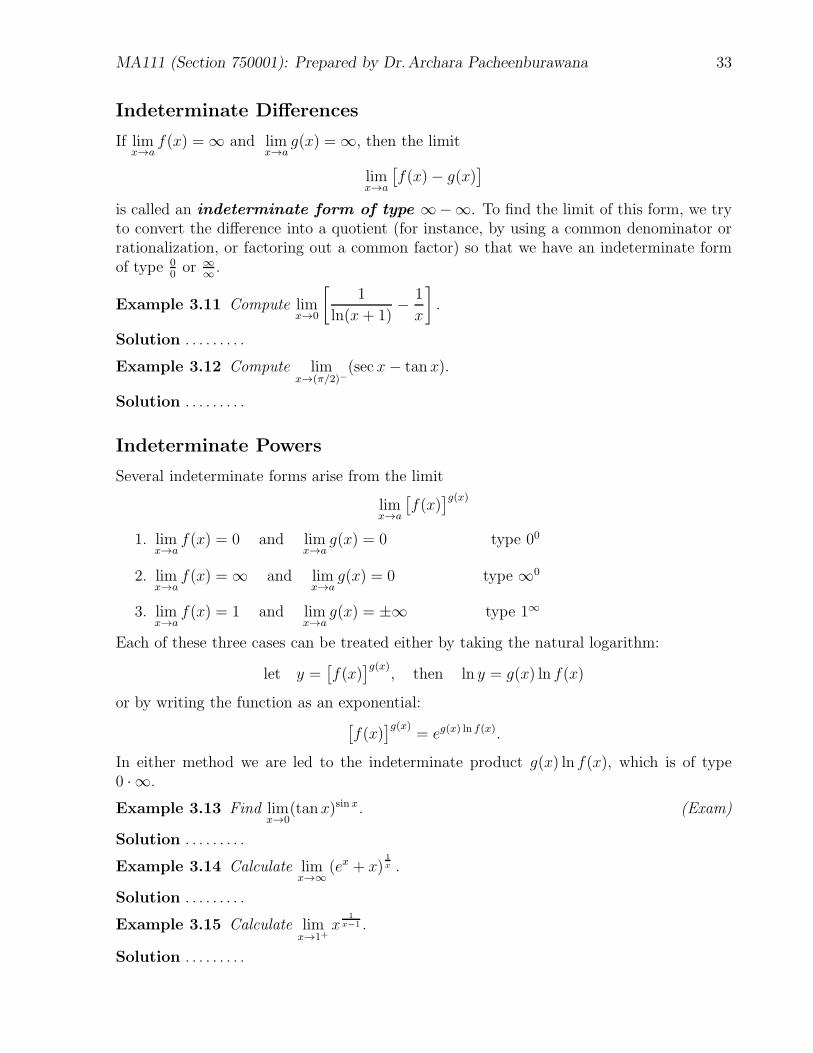
Indeterminate Differences

If limx→a

f(x) = ∞ and limx→a

g(x) = ∞, then the limit

limx→a

[

f(x)− g(x)]

is called an indeterminate form of type ∞−∞. To find the limit of this form, we tryto convert the difference into a quotient (for instance, by using a common denominator orrationalization, or factoring out a common factor) so that we have an indeterminate formof type 0

0or ∞

∞ .

Example 3.11 Compute limx→0

[

1

ln(x+ 1)− 1

x

]

.

Solution . . . . . . . . .

Example 3.12 Compute limx→(π/2)−

(sec x− tan x).

Solution . . . . . . . . .

Indeterminate Powers

Several indeterminate forms arise from the limit

limx→a

[

f(x)]g(x)

1. limx→a


g(x) = 0 type 00

2. limx→a

f(x) = ∞ and limx→a

g(x) = 0 type ∞0

3. limx→a


g(x) = ±∞ type 1∞

Each of these three cases can be treated either by taking the natural logarithm:

let y =[

f(x)]g(x)

, then ln y = g(x) ln f(x)

or by writing the function as an exponential:[

f(x)]g(x)

= eg(x) ln f(x).

In either method we are led to the indeterminate product g(x) ln f(x), which is of type0 · ∞.

Example 3.13 Find limx→0

(tanx)sinx. (Exam)

Solution . . . . . . . . .

Example 3.14 Calculate limx→∞

(ex + x)1

x .

Solution . . . . . . . . .

Example 3.15 Calculate limx→1+

x1

x−1 .

Solution . . . . . . . . .


3.3 Maximum and Minimum Values of a Function

Some of the most important applications of differential calculus are optimization problems,in which we are required to find the optimal (best) way of doing something. Here areexamples of such problems:

• A farmer wants to choose the mix of crops that is likely to produce the largest profit.

• A doctor wishes to select the smallest dosage of a drug that will cure certain disease.

• The manufacturer would like to minimize the cost of distributing its products.

These problems can be reduced to finding the maximum or minimum values of a function.Let’s first explain exactly what we mean by the maximum and minimum values.

Definition 3.1 A function f has an absolute maximum (or global maximum) at cif f(c) ≥ f(x) for all x in D, where D is the domain of f . The number f(c) is called themaximum value of f on D. Similarly, f has an absolute minimum at c if f(c) ≤ f(x)for all x in D and the number f(c) is called the minimum value of f on D. The maximumand minimum values of f are called the extreme values of f .

Figure 3.1 shows the graph of a function f with absolute maximum at b and absoluteminimum at e. Note that

(

b, f(b))

is the highest point on the graph and(

e, f(e))

is thelowest point.

x

y

a b c d e

b

b

(

b, f(b))

(

e, f(e))

Figure 3.1: Maximum value f(b), minimum value f(e)

In general, there is no guarantee that a function will actually have an absolute maximumor minimum on the given interval.

c

f(c)

y

x

b

y = f(x)

Minimum value at c, no maximum

c

f(c)

y

x

by = f(x)

Maximum value at c, no minimum


The following theorem gives conditions under which a function is guaranteed to possesextreme values

Theorem 3.2 (Extreme Value Theorem)

If f is continuous on a closed interval [a, b], then f attains an absolute maximum value f(c)and an minimum value f(d) at some numbers c and d in [a, b].

The Extreme Value Theorem is illustrated in the following Figure. Note that an extremevalue can be taken on more than once.

y

x

b

b

| |

a c d b

y

x

b

b

|

a c d = b

y

x

b

b

| |

a c1 d c2 b

The following Figure show that a function need not be possess extreme values if eitherhypothesis (continuity or closed interval) is omitted from the Extreme Value Theorem.

y

x

fb

b

bc

b|

+

0 2

1

3

This function has minimum value

f(2) = 0, but no maximum value.

y

x

g

1

1 bc

0

This continuous function g has

no maximum and minimum.

The Extreme Value Theorem says that a continuous function on a closed interval hasa maximum value and a minimum value, but it does not tell us how to find these extremevalues. We start by looking for local extreme values.

Definition 3.2 A function f has a local maximum (or relative maximum) at c iff(c) ≥ f(x) when x is near c [This means that f(c) ≥ f(x) for all x in some open intervalcontaining c.] Similarly, f has a local minimum at c if f(c) ≤ f(x) when x is near c.If f has either a local maximum or a local minimum at c, then f is said to have a local

extreme values at c.


y

xab

cd

b

b

b

b

Local max[f ′(a) does not exist]

Local minf ′(b) does not exist

Local max[f ′(c) = 0]

Local min[f ′(d) = 0]

Figure 3.2: Local extreme values

Figure 3.2 illustrates that a local extreme value can occur at a point in the domain offunction at which either the graph of the function has a horizontal tangent line or functionis not differentiable.

Definition 3.3 A critical number of a function f is a number c in the domain of f suchthat f ′(c) = 0 or f ′(c) does not exist.

Theorem 3.3 (Fermat’s Theorem) If f has a local maximum or minimum at c, then cis a critical number of f .

Example 3.16 Find all critical numbers and the local extreme values of

f(x) = 2x3 + 3x2 − 12x− 5.

Solution . . . . . . . . .

Example 3.17 Find all critical numbers and the local extreme values of f(x) = (2x+3)2/3.

Solution . . . . . . . . .

Fermat’s Theorem does suggest that we should at least start looking for extreme valuesof f at a critical number of f .

Example 3.18 Find the critical numbers of

f(x) =x2 + 3

x+ 1.

Solution . . . . . . . . .

To find an absolute maximum or minimum of a continuous function on a closed interval,we note that either it is local [in which case it occurs at a critical number] or it occurs atan endpoint of the interval. Thus the following three-step procedure always works.


The Closed Interval Method

To find the absolute maximum and minimum values of a continuous function f on a closedinterval [a, b]:

1. Find the critical points of f in (a, b)

2. Evaluate f at all the critical numbers and at the endpoints a and b.

3. The largest of the values in Step 2 is the absolute maximum value of f on [a, b] andthe smallest value is the absolute minimum.

Example 3.19 Find the absolute maximum and absolute minimum values of the function

f(x) = x3 − 3x+ 1

on the interval [0, 3].

Solution . . . . . . . . .

Example 3.20 Find the absolute maximum and absolute minimum values of the function

f(x) =ln x

x1 ≤ x ≤ 3.

Solution . . . . . . . . .

3.4 Increasing and Decreasing Functions

Definition 3.4 Let f be defined on an interval I (open, closed, or neither), and let x1 andx2 denote points in I.

(a) f is increasing on I if f(x1) < f(x2) whenever x1 < x2.

(b) f is decreasing on I if f(x1) > f(x2) whenever x1 < x2.

(c) f is constant on I if f(x1) = f(x2) for all points x1 and x2.

Theorem 3.4 (Increasing/Decreasing Test) Let f be continuous on an interval I anddifferentiable at every interior point of I.

(i) If f ′(x) > 0 for all x interior to I, then f is increasing on I.

(ii) If f ′(x) < 0 for all x interior to I, then f is decreasing on I.

(iii) If f ′(x) = 0 for all x in I, then f is constant on I.

Example 3.21 Find the interval on which f(x) = 3x4 + 4x3 − 12x2 − 5 is increasing andthe interval on which it is decreasing.

Solution . . . . . . . . .


Theorem 3.5 (First Derivative Test)

Let f be continuous on an open interval (a, b) that contains a critical number c.

1. If f ′(x) > 0 for all x ∈ (a, c) and f ′(x) < 0 for all x ∈ (c, b), then f(c) is a localmaximum value of f .

2. If f ′(x) < 0 for all x ∈ (a, c) and f ′(x) > 0 for all x ∈ (c, b), then f(c) is a localminimum value of f .

3. If f ′(x) has the same sign on both sides of c, then f(c) is not a local extreme value off .

It is easy to remember the First Derivative Test by visualizing diagram such as those inthe following Figure.

y

x0 c

f ′(x) > 0 f ′(x) < 0

(a) Local maximum

y

x0 c

f ′(x) < 0 f ′(x) > 0

(b) Local minimum

y

x0 c

f ′(x) > 0

f ′(x) > 0

(c) No maximum or minimum

y

x0 c

f ′(x) < 0

f ′(x) < 0

(d) No maximum or minimum

Example 3.22 Find the local minimum and maximum values of the function f(x) = xex.

Solution . . . . . . . . .

Example 3.23 Find the local minimum and maximum values of f(x) = x(x− 1)3.

Solution . . . . . . . . .

3.5 Concavity

Definition 3.5 Let f be differentiable on an open interval I. We say that f (as well as itsgraph) is concave up on I if f ′ is increasing on I and we say that f is concave down

on I if f ′ is decreasing on I.


Theorem 3.6 (Concavity Test)

Let f be twice differentiable on an open interval I.

1. If f ′′ > 0 for all x in I, then f is concave up on I.

2. If f ′′ < 0 for all x in I, then f is concave down on I.

Definition 3.6 Let f be continuous at c. We call (c, f(c)) an inflection point of thegraph f if f is concave up on one side of c and concave down on the other side.

Example 3.24 Let f(x) = x4 − 6x2 + 3. Find the intervals of concavity and the inflectionpoints.

Solution . . . . . . . . .

Theorem 3.7 (The Second Derivative Test) Let f ′ and f ′′ exist at every point in anopen interval (a, b) containing c, and suppose f ′(c) = 0.

1. If f ′′(c) < 0, then f(c) is a local maximum value of f .

2. If f ′′(c) > 0, then f(c) is a local minimum value of f .

Example 3.25 For f(x) = 2x3 +6x2 − 18x+5, use the Second Derivative Test to identifylocal extrema.

Solution . . . . . . . . .

Note. The Second Derivative Test is inconclusive when f ′′(c) = 0. In other words, at sucha point there might be a maximum, there might be a minimum, or there be neither. Thistest also fails when f ′′(c) dost not exist. In such cases the The First Derivative Test mustbe used. In fact, even when both tests apply, the First Derivative Test is often the easierone to use.

Example 3.26 Let f(x) = x4 − 4x3 + 10.

• Find the interval of increase and decrease.

• Find the local maximum and minimum values.

• Find the intervals of concavity and the inflection points.

• Use the above information to sketch the graph.

Solution . . . . . . . . .

Example 3.27 Let f(x) = x2/3(6− x)1/3.






Solution . . . . . . . . .

Example 3.28 Let f(x) =x2

√x+ 1

.





Solution . . . . . . . . .

Chapter 1 Limits and Continuity

Documents

Transcript of Chapter 1 Limits and Continuity