Metric spaces and continuity - The Open University

M303

Further pure mathematics

Metric spaces and continuity

This publication forms part of an Open University module. Details of this and otherOpen University modules can be obtained from the Student Registration and Enquiry Service, TheOpen University, PO Box 197, Milton Keynes MK7 6BJ, United Kingdom (tel. +44 (0)845 300 6090;email [email protected]).

Alternatively, you may visit the Open University website at www.open.ac.uk where you can learnmore about the wide range of modules and packs offered at all levels by The Open University.

Note to reader

Mathematical/statistical content at the Open University is usually provided to students inprinted books, with PDFs of the same online. This format ensures that mathematical notationis presented accurately and clearly. The PDF of this extract thus shows the content exactly asit would be seen by an Open University student. Please note that the PDF may containreferences to other parts of the module and/or to software or audio-visual components of themodule. Regrettably mathematical and statistical content in PDF files is unlikely to beaccessible using a screenreader, and some OpenLearn units may have PDF files that are notsearchable. You may need additional help to read these documents.

The Open University, Walton Hall, Milton Keynes, MK7 6AA.

First published 2014. Second edition 2016.

Copyright c© 2014, 2016 The Open University

All rights reserved. No part of this publication may be reproduced, stored in a retrieval system, transmittedor utilised in any form or by any means, electronic, mechanical, photocopying, recording or otherwise, withoutwritten permission from the publisher or a licence from the Copyright Licensing Agency Ltd. Details of suchlicences (for reprographic reproduction) may be obtained from the Copyright Licensing Agency Ltd, SaffronHouse, 6–10 Kirby Street, London EC1N 8TS (website www.cla.co.uk).

Open University materials may also be made available in electronic formats for use by students of theUniversity. All rights, including copyright and related rights and database rights, in electronic materials andtheir contents are owned by or licensed to The Open University, or otherwise used by The Open University aspermitted by applicable law.

In using electronic materials and their contents you agree that your use will be solely for the purposes offollowing an Open University course of study or otherwise as licensed by The Open University or its assigns.

Except as permitted above you undertake not to copy, store in any medium (including electronic storage oruse in a website), distribute, transmit or retransmit, broadcast, modify or show in public such electronicmaterials in whole or in part without the prior written consent of The Open University or in accordance withthe Copyright, Designs and Patents Act 1988.

Edited, designed and typeset by The Open University, using the Open University TEX System.

Printed in the United Kingdom by Halstan & Co. Ltd, Amersham, Bucks.

ISBN 978 1 4730 2036 8

2.1

Contents

Contents

1 Introducing metric spaces 5

1.1 The definition of a metric space 5

1.2 Examples of metric spaces 7

1.3 Understanding the geometry of metric spaces 12

16

19

23

2 Sequences in metric spaces

3 The definition of continuity in metric spaces

Solutions and comments on exercises

Index 27

1 Introducing metric spaces


We now introduce the idea of a metric space, and show how this conceptallows us to generalise the notion of continuity. We will then concentrateon looking at some examples of metric spaces and defer further discussionof continuous functions between metric spaces to the next chapter. You should not expect to have a

firm grasp of the idea of a metricspace by the end of this section:this will come as you see moreexamples of metric spaces inChapter 15 and later chapters.

Subsection 1.1 shows how properties of the Euclidean distance function onRn can be generalised to define a metric on any set to create a metric

space.

1.1 The definition of a metric space

Looking back at the definition of continuity for functions from Rn to R

m

we see that it depends on:

• the Euclidean distance in Rn, d(n) Recall that if a,b ∈ R

k, then

d(k)(a,b) is given by√

∑

k

i=1(bi − ai)2.• the Euclidean distance in R

m, d(m)

• the definition of convergence for sequences in both Rn and R

m.

Moreover, the definition of convergence for sequences also depends on thenotion of distance. Thus a notion of distance (in both the domain and thecodomain) is a fundamental part of our definition of continuity. Hence todefine a notion of continuity for functions between arbitrary sets X and Y ,we must first have effective notions of distance appropriate to the sets Xand Y . An obvious strategy to do this is to try to find some properties ofthe Euclidean distance that we would expect any sensible notion ofdistance to possess.

We showed that the Euclidean distance function has three properties.

The Euclidean distance function d(n) : Rn × Rn → R has the following

properties.

For each a,b, c ∈ Rn:

(M1) d(n)(a,b) ≥ 0, with equality holding if, and only if, a = b

(M2) d(n)(a,b) = d(n)(b,a)

(M3) d(n)(a, c) ≤ d(n)(a,b) + d(n)(b, c) (the Triangle Inequality).

Properties (M1)–(M3) do not use any special properties of the set Rn, so itseems reasonable to say that for any set X, a function d : X ×X → R is adistance function if it satisfies them. It turns out that these are indeed theappropriate properties of distance on which to base our definition. We callsuch a distance function a metric, and we call a set with such a functiondefined on it a metric space. The word metric comes from the

Greek word µετρoν (metron),meaning ‘measure’, aninstrument for measuring.

5

Metric spaces and continuity 1

Definition 1.1 Metric

Let X be a set. A metric on X is a function d : X ×X → R thatsatisfies the following three conditions.

For each a, b, c ∈ X:

(M1) d(a, b) ≥ 0, with equality holding if, and only if, a = b

(M2) d(a, b) = d(b, a)(M3) d(a, c) ≤ d(a, b) + d(b, c) (the Triangle Inequality).

The set X, together with a metric d on X, is called a metric space,and is denoted by (X, d).This definition was proposed by

Maurice Frechet, whose work isdiscussed in the History Reader.

Remarks

1. Mathematicians usually refer to the members of the set X as points,A ‘point’ may be nothing like adot in the plane: X could be aset of functions and then a pointin X would be a function.

to emphasise the analogy with the points of a line, a plane orthree-dimensional space. Similarly, mathematicians usually refer tod(a, b) as the distance between a and b. The theory of metric spacesis the study of those properties of sets of points that depend only ondistance.

2. Condition (M1) says that distance is a non-negative quantity, and thatthe only point of a metric space that is at zero distance from a givenpoint is that point itself.

3. Condition (M2) says that the distance from a point a to a point b isprecisely the same as the distance from b to a. (The metric issymmetric. It doesn’t matter whether you are going from a to b orfrom b to a – the distance is the same.)

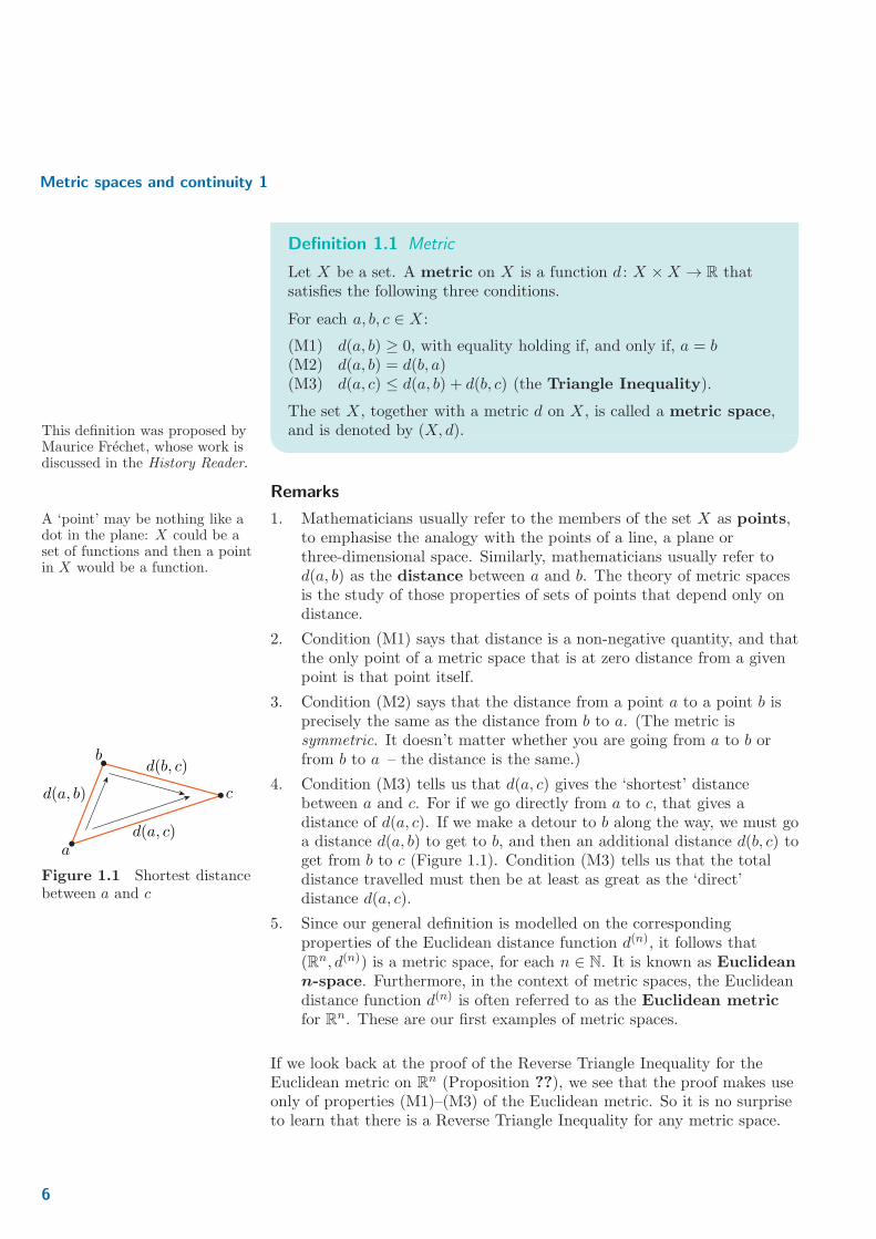
4. Condition (M3) tells us that d(a, c) gives the ‘shortest’ distancebetween a and c. For if we go directly from a to c, that gives adistance of d(a, c). If we make a detour to b along the way, we must goa distance d(a, b) to get to b, and then an additional distance d(b, c) toget from b to c (Figure 1.1). Condition (M3) tells us that the total

b

d(a, b)

d(b, c)

d(a, c)

c

a

Figure 1.1 Shortest distancebetween a and c

distance travelled must then be at least as great as the ‘direct’distance d(a, c).

5. Since our general definition is modelled on the correspondingproperties of the Euclidean distance function d(n), it follows that(Rn, d(n)) is a metric space, for each n ∈ N. It is known as Euclidean

n-space. Furthermore, in the context of metric spaces, the Euclideandistance function d(n) is often referred to as the Euclidean metric

for Rn. These are our first examples of metric spaces.

If we look back at the proof of the Reverse Triangle Inequality for theEuclidean metric on R

n (Proposition ??), we see that the proof makes useonly of properties (M1)–(M3) of the Euclidean metric. So it is no surpriseto learn that there is a Reverse Triangle Inequality for any metric space.

6


Proposition 1.2 Reverse Triangle Inequality for metric spaces

Let (X, d) be a metric space. For each a, b, c ∈ X,(M3a) d(b, c) ≥ |d(a, c) − d(a, b)|. The proof is essentially the same

as that for Proposition ??, andso we omit it.

1.2 Examples of metric spaces

We now give a few examples of metric spaces with the aim of getting youused to showing that a distance function is a metric. The examples weconsider here are not very sophisticated and may not persuade you of theutility of this new concept. However, in the next chapter we investigateways of defining distances between more interesting ‘points’, such asbetween pairs of functions or pairs of sequences – this is when we will startto see the real power of metrics.

The discrete metric

Our first example is simple but important, since it shows that it is possibleto define a metric on any set X.

Definition 1.3 Discrete metric

Let X be a set. The discrete metric on X is the functiond0 : X ×X → R defined by

d0(a, b) =

{

0, if a = b,

1, if a 6= b.We show that d0 is a metricafter the remarks.

Remarks

1. When X = ∅, the empty set, the definition still makes sense but is notvery interesting.

2. The d0-distance between any two distinct points of a set X is alwaysequal to 1. In particular, if we consider the case when X = R, the realline, we find that d0 is a different metric from the usual Euclideandistance. (To see this, observe that d0(0, 2) = 1 whereas

d(1)(0, 2) = 2.) Thus the discrete metric gives us a second notion ofdistance on R. In fact, if (X, d) is any metric space whose metric d isnot d0, then (X, d0) is a second metric space with underlying set X.

The discrete metric is about the simplest possible notion of distancethere can be and acts to ‘isolate’ points of a space: they are all atdistance 1 from one another.

7


Proposition 1.4

Let X be a set. Then (X, d0) is a metric space.

Proof Let X be a set. In order to show that d0 is a metric on X, wemust show that d0 satisfies conditions (M1)–(M3).

If X = ∅, then X has no elements and so each of (M1)–(M3) vacuouslyholds: there is nothing to prove. So suppose instead that X is non-empty.

(M1) Since d0 can take only the values 0 and 1, we have d0(a, b) ≥ 0 foreach choice of a, b ∈ X.

The definition of d0 implies immediately that d0(a, b) = 0 if, and onlyif, a = b.

Thus d0 satisfies (M1).

(M2) If a = b, then d0(a, b) = 0 = d0(b, a).

If a 6= b, then d0(a, b) = 1 = d0(b, a).

Thus, for each a, b ∈ X, (M2) holds.

(M3) Let a, b, c ∈ X. We examine the two possible cases: d0(a, c) = 0 andd0(a, c) = 1.

Suppose d0(a, c) = 0 (so a = c). Since d0(a, b) and d0(b, c) arenon-negative, it follows that

d0(a, b) + d0(b, c) ≥ 0 = d0(a, c).

Now suppose d0(a, c) = 1; then a 6= c and so b cannot equal both a

and c. Hence, from (M1), at least one of d0(a, b) and d0(b, c) isnon-zero and so must equal 1. Thus

d0(a, b) + d0(b, c) ≥ 1 = d0(a, c).

Hence, in both cases, (M3) holds.

Since d0 satisfies (M1)–(M3), it is a metric on X and (X, d0) is a metricspace.

At first appearance, the simplicity of the definition of the discrete metricd0 may make it seem unimportant, but this is not the case. Its utility liesin the fact that it gives an ‘extreme’ example of a metric space – no otherdefinition of distance so completely ignores any structure that may bepresent in the underlying set X.

We use the discrete metric for a number of purposes, principally to testproperties that we suspect may hold for all metric spaces. If such aproperty fails for (X, d0), then we know that our suspicion was false.

8


Exercise 1.1

Let X = {x, y, z} and define d : X ×X → R by

d(x, x) = d(y, y) = d(z, z) = 0,

d(x, y) = d(y, x) = 1,

d(y, z) = d(z, y) = 2,

d(x, z) = d(z, x) = 4.

Determine whether d is a metric on X.

The taxicab metric: an alternative metric for the plane

We have already observed that the usual definition of distance on the planedefines a metric and we have just seen that it is possible to define a verysimple notion of distance on the plane, namely the discrete metric givenpreviously. Here we introduce another natural way to measure distancebetween points in the plane, the taxicab metric.

Recall that the usual definition of distance on the plane is given by

d(2)(a,b) =√

(b1 − a1)2 + (b2 − a2)2 for a,b ∈ R2.

What happens if we change the formula we use for distance on theright-hand side of this expression to something that is perhaps easier tocalculate? For example, consider the function e1 : R

2 × R2 → R defined by The reason for the subscript 1 in

the notation e1 will becomeclear in Chapter 15.e1(a,b) = |b1 − a1|+ |b2 − a2| for a,b ∈ R

2.

As we will shortly see, this does define an alternative metric on the plane.First let us understand how this distance function behaves.

Exercise 1.2

Find:

(a) e1((0, 0), (1, 0)); (b) e1((0, 0), (0, 1));

(c) e1((0, 1), (1, 0)).

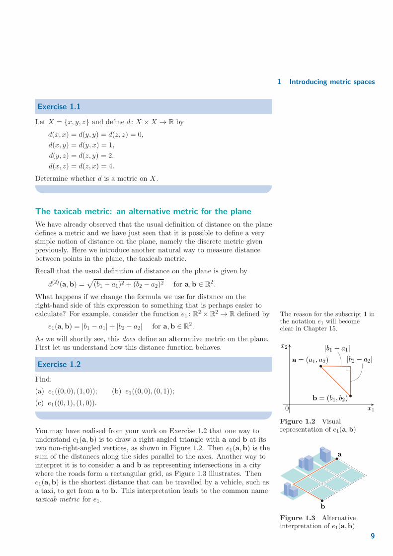
You may have realised from your work on Exercise 1.2 that one way tounderstand e1(a,b) is to draw a right-angled triangle with a and b at itstwo non-right-angled vertices, as shown in Figure 1.2. Then e1(a,b) is the

x2

0

a = (a1, a2)

b = (b1, b2)

|b1 − a1||b2 − a2|

x1

Figure 1.2 Visualrepresentation of e1(a,b)

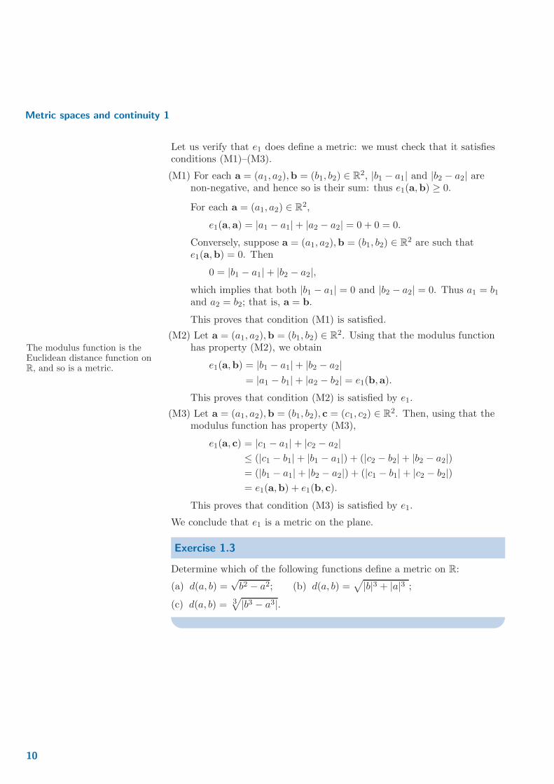
sum of the distances along the sides parallel to the axes. Another way tointerpret it is to consider a and b as representing intersections in a citywhere the roads form a rectangular grid, as Figure 1.3 illustrates. Then

a

b

Figure 1.3 Alternativeinterpretation of e1(a,b)

e1(a,b) is the shortest distance that can be travelled by a vehicle, such asa taxi, to get from a to b. This interpretation leads to the common nametaxicab metric for e1.

9


Let us verify that e1 does define a metric: we must check that it satisfiesconditions (M1)–(M3).

(M1) For each a = (a1, a2),b = (b1, b2) ∈ R2, |b1 − a1| and |b2 − a2| are

non-negative, and hence so is their sum: thus e1(a,b) ≥ 0.

For each a = (a1, a2) ∈ R2,

e1(a,a) = |a1 − a1|+ |a2 − a2| = 0 + 0 = 0.

Conversely, suppose a = (a1, a2),b = (b1, b2) ∈ R2 are such that

e1(a,b) = 0. Then

0 = |b1 − a1|+ |b2 − a2|,which implies that both |b1 − a1| = 0 and |b2 − a2| = 0. Thus a1 = b1and a2 = b2; that is, a = b.

This proves that condition (M1) is satisfied.

(M2) Let a = (a1, a2),b = (b1, b2) ∈ R2. Using that the modulus function

has property (M2), we obtainThe modulus function is theEuclidean distance function onR, and so is a metric. e1(a,b) = |b1 − a1|+ |b2 − a2|

= |a1 − b1|+ |a2 − b2| = e1(b,a).

This proves that condition (M2) is satisfied by e1.

(M3) Let a = (a1, a2),b = (b1, b2), c = (c1, c2) ∈ R2. Then, using that the

modulus function has property (M3),

e1(a, c) = |c1 − a1|+ |c2 − a2|≤ (|c1 − b1|+ |b1 − a1|) + (|c2 − b2|+ |b2 − a2|)= (|b1 − a1|+ |b2 − a2|) + (|c1 − b1|+ |c2 − b2|)= e1(a,b) + e1(b, c).

This proves that condition (M3) is satisfied by e1.

We conclude that e1 is a metric on the plane.

Exercise 1.3

Determine which of the following functions define a metric on R:

(a) d(a, b) =√b2 − a2; (b) d(a, b) =

√

|b|3 + |a|3 ;

(c) d(a, b) = 3√

|b3 − a3|.

10


A ‘mixed’ metric in the plane

Our next example of a metric is a mixture of the discrete metric and themodulus function.

For points a = (a1, a2), b = (b1, b2) in the plane, define the functiond : R2 × R

2 → R by

d(a,b) = |b1 − a1|+ d0(a2, b2),

where d0 denotes the discrete metric on R.

Our goal is to show that this is indeed a metric on the plane. To do this,we make extensive use of the fact that the modulus function and thediscrete metric both satisfy properties (M1)–(M3) on R.

Exercise 1.4

Show that d has property (M1).

Exercise 1.5


We verify the Triangle Inequality as a worked exercise.

Worked Exercise 1.5


Solution

We must show that for any choice of a, b, c ∈ R2, we have

d(a, c) ≤ d(a,b) + d(b, c).

As with the previous exercises, we use the fact that both | · | and d0have property (M3) when viewed as metrics on R.

Let a = (a1, a2), b = (b1, b2), c = (c1, c2) ∈ R2. Then

d(a, c) = |a1 − c1|+ d0(c2, a2), by the definition of d

≤ |a1 − b1|+ |b1 − c1|+ d0(c2, a2), by (M3) for | · |≤ |a1 − b1|+ |b1 − c1|+ d0(c2, b2) + d0(b2, a2), by (M3) for d0

= (|a1 − b1|+ d0(b2, a2)) + (|b1 − c1|+ d0(c2, b2))

= d(a,b) + d(b, c),

as required.

Since d has properties (M1)–(M3), we conclude that it is a metric for R2

but rather a strange one!

11


1.3 Understanding the geometry of metric spaces

Before we look at what it means for a sequence to be convergent withrespect to a given metric, we spend a little time discussing one way ofgaining some understanding about the geometric meaning of a givenmetric.

In the last subsection, we met three different metrics: the discrete metric,the taxicab metric on the plane and a mixed metric on the plane (whichwas formed from the usual distance in R together with the discrete metric).

An easy way to gain some insight into the behaviour of a metric is to lookat the balls around a given point. For the usual Euclidean distance in R

n,a ball of radius r around a point a ∈ R

n consists of all those points whosedistance from a is at most r, and this definition naturally extends togeneral metric spaces. However, in the following definition we take care todistinguish between balls that include points at exactly distance r from thecentre a and those that do not.

Definition 1.6 Open and closed balls

Let (X, d) be a metric space, and let a ∈ X and r ≥ 0.

The open ball of radius r with centre a is the set

Bd(a, r) = {x ∈ X : d(a, x) < r}.The closed ball of radius r with centre a is the set

Bd[a, r] = {x ∈ X : d(a, x) ≤ r}.The sphere of radius r with centre a is the set

Sd(a, r) = {x ∈ X : d(a, x) = r}.When r = 1, these sets are called respectively the unit open ball

with centre a, the unit closed ball with centre a and the unit

sphere with centre a.There is no universal agreementon the terminology and notationfor balls. It is a wise precautionto check the conventionswhenever reading a book onmetric spaces.

Remarks

1. When we wish to emphasise the particular metric d on X, we refer tothe d-open ball , the d-closed ball and the d-sphere.

2. When d is the usual Euclidean metric on R2, we recover the usual

notions of open and closed balls in the plane.

3. Since d(a, a) = 0, a ∈ Bd(a, r) whenever r > 0 and a ∈ Bd[a, r]whenever r ≥ 0.

12


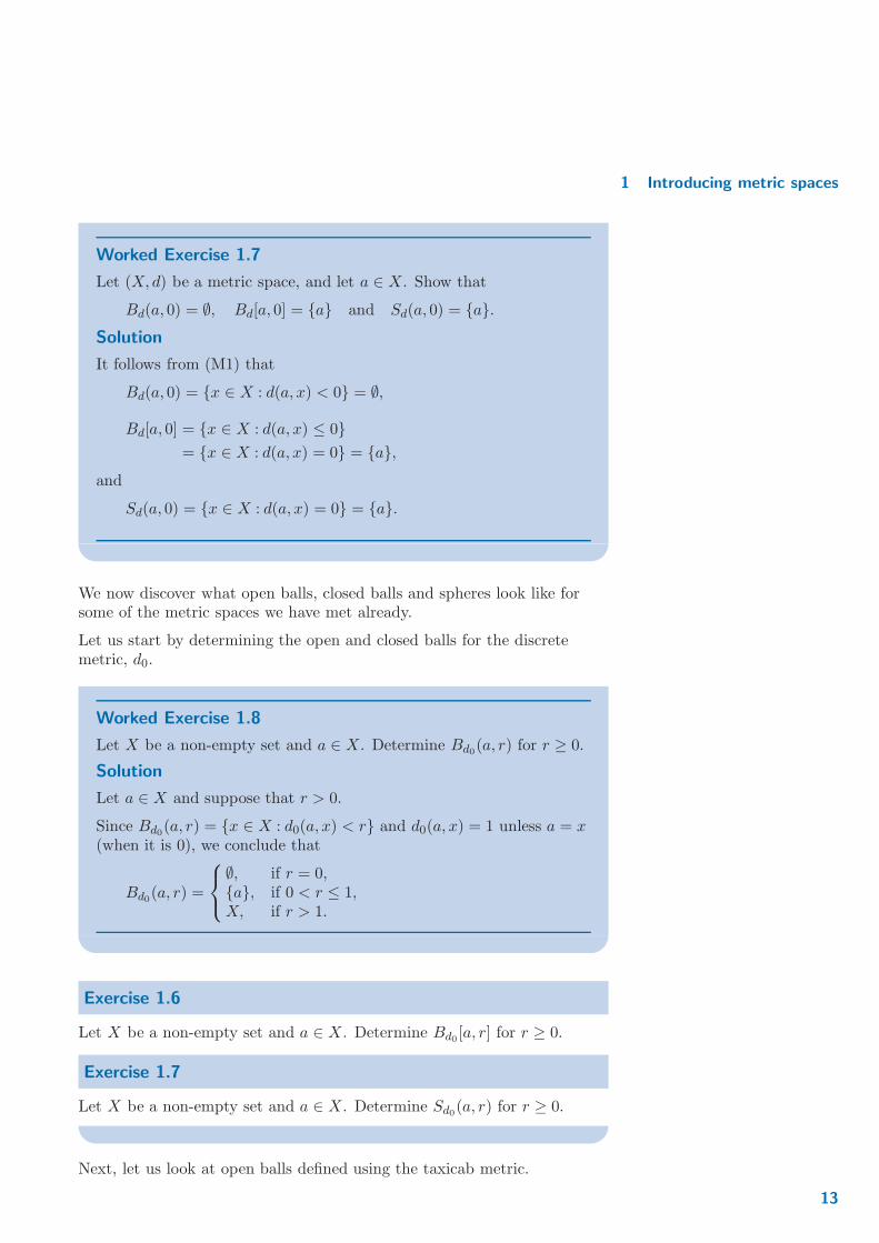
Worked Exercise 1.7

Let (X, d) be a metric space, and let a ∈ X. Show that

Bd(a, 0) = ∅, Bd[a, 0] = {a} and Sd(a, 0) = {a}.Solution

It follows from (M1) that

Bd(a, 0) = {x ∈ X : d(a, x) < 0} = ∅,

Bd[a, 0] = {x ∈ X : d(a, x) ≤ 0}= {x ∈ X : d(a, x) = 0} = {a},

and

Sd(a, 0) = {x ∈ X : d(a, x) = 0} = {a}.

We now discover what open balls, closed balls and spheres look like forsome of the metric spaces we have met already.

Let us start by determining the open and closed balls for the discretemetric, d0.

Worked Exercise 1.8

Let X be a non-empty set and a ∈ X. Determine Bd0(a, r) for r ≥ 0.

Solution

Let a ∈ X and suppose that r > 0.

Since Bd0(a, r) = {x ∈ X : d0(a, x) < r} and d0(a, x) = 1 unless a = x

(when it is 0), we conclude that

Bd0(a, r) =

∅, if r = 0,{a}, if 0 < r ≤ 1,X, if r > 1.

Exercise 1.6

Let X be a non-empty set and a ∈ X. Determine Bd0 [a, r] for r ≥ 0.

Exercise 1.7

Let X be a non-empty set and a ∈ X. Determine Sd0(a, r) for r ≥ 0.

Next, let us look at open balls defined using the taxicab metric.

13


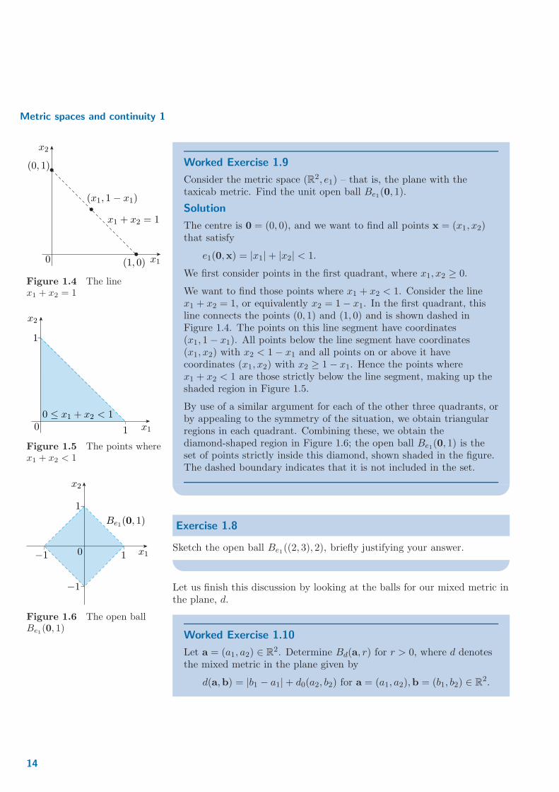
Worked Exercise 1.9

Consider the metric space (R2, e1) – that is, the plane with thetaxicab metric. Find the unit open ball Be1(0, 1).

Solution

The centre is 0 = (0, 0), and we want to find all points x = (x1, x2)that satisfy

e1(0,x) = |x1|+ |x2| < 1.

We first consider points in the first quadrant, where x1, x2 ≥ 0.

x2

(0, 1)

0

(x1, 1− x1)

x1 + x2 = 1

(1, 0) x1

Figure 1.4 The linex1 + x2 = 1 We want to find those points where x1 + x2 < 1. Consider the line

x1 + x2 = 1, or equivalently x2 = 1− x1. In the first quadrant, thisline connects the points (0, 1) and (1, 0) and is shown dashed inFigure 1.4. The points on this line segment have coordinates(x1, 1− x1). All points below the line segment have coordinates(x1, x2) with x2 < 1− x1 and all points on or above it havecoordinates (x1, x2) with x2 ≥ 1− x1. Hence the points wherex1 + x2 < 1 are those strictly below the line segment, making up theshaded region in Figure 1.5.

x2

00 ≤ x1 + x2 < 1

1

1

x1

Figure 1.5 The points wherex1 + x2 < 1

By use of a similar argument for each of the other three quadrants, orby appealing to the symmetry of the situation, we obtain triangularregions in each quadrant. Combining these, we obtain thediamond-shaped region in Figure 1.6; the open ball Be1(0, 1) is theset of points strictly inside this diamond, shown shaded in the figure.The dashed boundary indicates that it is not included in the set.

−1

−1

x2

0

Be1(0, 1)

x1

1

1

Figure 1.6 The open ballBe1

(0, 1)

Exercise 1.8

Sketch the open ball Be1((2, 3), 2), briefly justifying your answer.

Let us finish this discussion by looking at the balls for our mixed metric inthe plane, d.

Worked Exercise 1.10

Let a = (a1, a2) ∈ R2. Determine Bd(a, r) for r > 0, where d denotes

the mixed metric in the plane given by

d(a,b) = |b1 − a1|+ d0(a2, b2) for a = (a1, a2),b = (b1, b2) ∈ R2.

14


Solution

Let a = (a1, a2) ∈ R2 and suppose that r > 0. Then, using the

definition of an open ball,

Bd(a, r) = {x = (x1, x2) ∈ R2 : d(a,x) < r}

= {x = (x1, x2) ∈ R2 : |x1 − a1|+ d0(a2, x2) < r}.

We now consider the cases x2 = a2 and x2 6= a2 separately. If x2 = a2,then d0(a2, x2) = 0 and so

{x = (x1, a2) ∈ R2 : |x1 − a1| < r} = {x1 ∈ R : |x1 − a1| < r} × {a2}

= (a1 − r, a1 + r)× {a2}.If x2 6= a2, then d0(a2, x2) = 1 and

{x = (x1, x2) ∈ R2 : x2 6= a2 and |x1 − a1|+ d0(a2, x2) < r}

= {x = (x1, x2) ∈ R2 : x2 6= a2 and |x1 − a1| < r − 1}.

Let us unpack this set expression: x2 can be any value other than a2but if r ≤ 1, then there are no possible x1 for which |x1 − a1| < r − 1,and so the expression is the empty set, ∅. Whereas if r > 1, then theset of x1 ∈ R for which |x1 − a1| < r − 1 is the interval(a1 − (r − 1), a1 + (r − 1)). Hence for r > 1, the set expression is(a1 − (r − 1), a1 + (r − 1))× (R− {a2}). Summarising,

{x = (x1, x2) ∈ R2 : x2 6= a2 and |x1 − a1|+ d0(a2, x2) < r}

=

{

∅, if r ≤ 1,(a1 − (r − 1), a1 + (r − 1))× (R − {a2}), if r > 1.

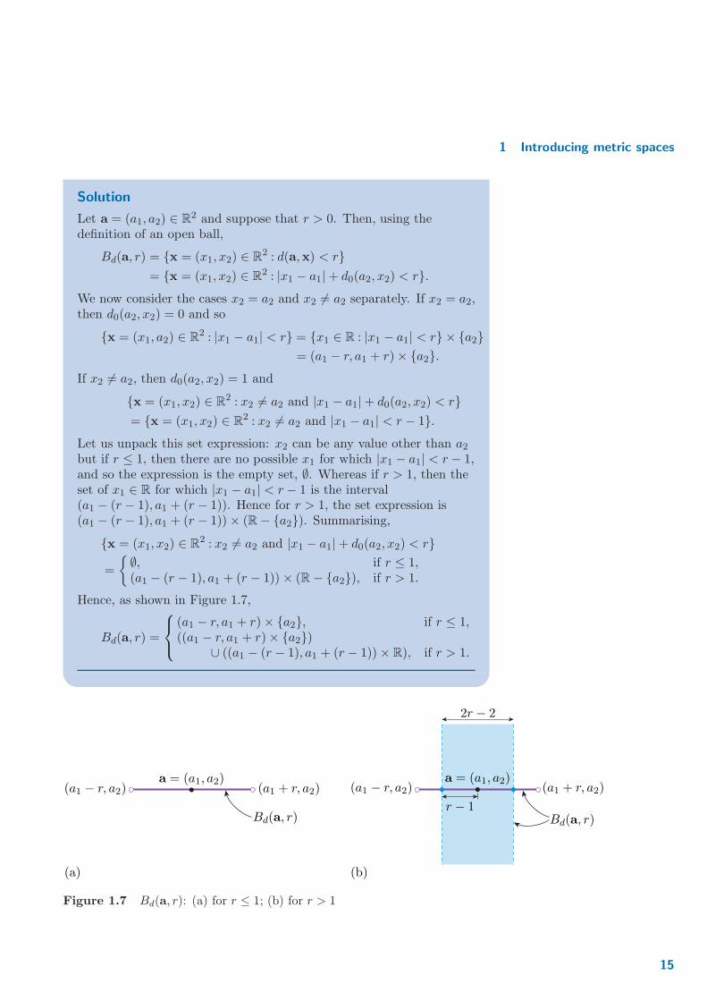
Hence, as shown in Figure 1.7,

Bd(a, r) =

(a1 − r, a1 + r)× {a2}, if r ≤ 1,((a1 − r, a1 + r)× {a2})

∪ ((a1 − (r − 1), a1 + (r − 1))× R), if r > 1.

(a1 − r, a2)a = (a1, a2)

(a1 + r, a2)

Bd(a, r) Bd(a, r)

a = (a1, a2)(a1 − r, a2)

r − 1

(a1 + r, a2)

2r − 2

(a) (b)

Figure 1.7 Bd(a, r): (a) for r ≤ 1; (b) for r > 1

15


Exercise 1.9

Let a = (a1, a2) ∈ R2. Determine Bd[a, r] for r ≥ 0, where d denotes the

mixed metric in the plane given by

d(a,b) = |b1 − a1|+ d0(a2, b2) for a = (a1, a2),b = (b1, b2) ∈ R2.

We will return to our investigation of the geometry of metric spaces inChapter 16.


Now that we have several examples of metric spaces available to us, wereturn to the problem of defining continuous functions between metricspaces.

Since the definition of a general metric space is modelled on the propertiesof the Euclidean metric d(n) on R

n, and we defined continuity of functionsbetween Euclidean spaces in terms of convergent sequences, it is natural toattempt to extend our ideas about convergent sequences in R

n to generalmetric spaces. In fact, we did much of the hard work when we generalisedfrom the notion of convergence for real-valued sequences to that ofconvergence of sequences in R

n; it is now only a short step to develop theseconcepts for the metric space setting.

In Chapter 13, we observed that a real sequence can be thought of as afunction a : N → R, given by n 7→ an. Note that the only role played by R

here is as the codomain of the function a : N → R; the structure of Rbecomes relevant only when convergence is considered. Since the codomainof a function is simply a set, the following definition is a naturalgeneralisation.

Definition 2.1 Sequence in a metric space

Let X be a set. A sequence in X is an unending ordered list ofelements of X:

a1, a2, a3, . . . .

The element ak is the kth term of the sequence, and the wholesequence is denoted by (ak), (ak)

∞k=1 or (ak)k∈N.

Note that this definition of a sequence does not require that we impose anyadditional structure (such as a metric) on the set X.

16


The definition of what it means for a sequence to converge in a metricspace (X, d) is closely based on the definition of convergence in R

n.

Definition 2.2 Convergence in a metric space

Let (X, d) be a metric space. A sequence (ak) in X d-converges toa ∈ X if the sequence of real numbers (d(ak, a)) is a null sequence.

We write akd→ a as k → ∞, or simply ak → a if the context is clear.

We say that the sequence (ak) is convergent in (X, d) with limit a.

A sequence that does not converge (with respect to the metric d) toany point in X is said to be d-divergent.

Remarks

1. Note that the limit a must be a point in X. For example, if X is the It is not hard to check that thisdefines a metric on (0, 1) – wereturn to the general problem ofdefining metrics on subsets ofmetric spaces in the nextchapter.

open interval (0, 1) and we give it the usual notion of distanced(a, b) = |a− b|, then the sequence ( 1

n) is not d-convergent, since the

only possible choice of limit is 0 – which is not a point of X.

2. In order to show that a sequence (ak) converges to a for the metric d,we must show that d(ak, a) → 0 as k → ∞ – that is, for each ε > 0,there is an N ∈ N for which d(ak, a) < ε for all k > N .

Exercise 2.1

Let (R2, e1) be the plane with the taxicab metric, and let (an) be thesequence given by ak = (1 + 1

2k , 2− 12k ). Show that (ak) converges to (1, 2)

with respect to e1.

Convergent sequences in (Rn, d(n)) have unique limits – that is, a sequencecannot simultaneously converge to two different limits. The next resultestablishes this as a fact in any metric space.

Theorem 2.3 Uniqueness of limits in a metric space

Let (X, d) be a metric space and let a, b ∈ X. If (ak) is a sequence inX that d-converges to both a and b, then a = b.

17


Proof We use proof by contradiction.

Suppose that the sequence (ak) d-converges to both a and b in X, witha 6= b. Then by property (M1) of Definition 1.1 for d, d(a, b) > 0 and so ifwe let ε = 1

2d(a, b), then ε > 0.

Since we are supposing that the sequence (ak) converges to both a and b,the sequences of real numbers (d(ak, a)) and (d(ak, b)) are both null. Hencethere is N ∈ N for which d(ak, a) < ε and d(ak, b) < ε whenever k > N .

The Triangle Inequality (property (M3) for d) tells us that, for each k > N ,

d(a, b) ≤ d(a, ak) + d(ak, b) < ε+ ε = 2ε

= d(a, b),

by the definition of ε. But this is impossible; hence our initial assumptionthat a sequence could converge to two distinct limits must be wrong. Weconclude that any d-convergent sequence has a unique limit.

The next definition enables us to describe a particularly straightforwardtype of convergent sequence.

Definition 2.4 Eventually constant

Let (ak) be a sequence in a set X. We say that (ak) is eventuallyconstant if there is a ∈ X and N ∈ N such that ak = a wheneverk > N .

Worked Exercise 2.5

Let (X, d) be a metric space and let (ak) be a sequence in X that iseventually constant. Show that (ak) converges for d and state itslimit.

Solution

Since (ak) is eventually constant, there is a ∈ X and N ∈ N such thatak = a whenever k > N . Therefore

d(ak, a) = d(a, a) = 0, for each k > N.

Hence the sequence of real numbers (d(an, a)) is null, which means

that akd→ a as k → ∞. Thus the sequence (ak) is d-convergent with

limit a.

18


Convergence and the discrete metric

Let us consider the sequence (ak) in (R, d0) given by ak = 1k. We see that (R, d0) is the set of real numbers

with the discrete metric d0.d0(ak, 0) = d0

(

1k, 0)

= 1, for each k ∈ N,

so (ak) does not converge to 0 with respect to the discrete metric d0. Infact, this sequence (ak) is divergent for d0, because given any non-zerol ∈ R,

d0(ak, l) = d0(1k, l) = 1 for each k > 1

|l| .

On the other hand, we know that the sequence ( 1k) does converge to 0 with

respect to the Euclidean metric d(1) on R. The important conclusion todraw from this example is:

convergence depends on how we measure distance.

In other words, different metrics on the same set can give rise to differentconvergent sequences.

From the solution to Worked Exercise 2.5, we know that eventuallyconstant sequences (ak) in a metric space (X, d0) are d0-convergent. Thenext exercise asks you to show that the eventually constant sequences arethe only convergent sequences for the d0 metric on a set X.

Exercise 2.2

Let X be a set and d0 the discrete metric for X. Suppose that (ak) is asequence in X that is d0-convergent. Show that (ak) is an eventuallyconstant sequence.

3 The definition of continuity in

metric spaces

Now that we know what it means for a sequence to converge in a metricspace, we can formulate a definition of continuity for functions betweenmetric spaces.

19


Definition 3.1 Continuity for metric spaces

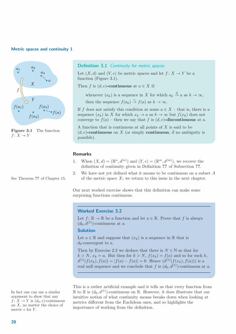
Let (X, d) and (Y, e) be metric spaces and let f : X → Y be afunction (Figure 3.1).

a1a2

a3

aX

f

Y

f(a1)

f(a2)

f(a3)

f(a)

Figure 3.1 The functionf : X → Y

Then f is (d, e)-continuous at a ∈ X if:

whenever (ak) is a sequence in X for which akd→ a as k → ∞,

then the sequence f(ak)e→ f(a) as k → ∞.

If f does not satisfy this condition at some a ∈ X – that is, there is asequence (xk) in X for which xk → a as k → ∞ but f(xk) does notconverge to f(a) – then we say that f is (d, e)-discontinuous at a.

A function that is continuous at all points of X is said to be(d, e)-continuous on X (or simply continuous, if no ambiguity ispossible).

Remarks

1. When (X, d) = (Rn, d(n)) and (Y, e) = (Rm, d(m)), we recover thedefinition of continuity given in Definition ?? of Subsection ??.

2. We have not yet defined what it means to be continuous on a subset Aof the metric space X; we return to this issue in the next chapter.See Theorem ?? of Chapter 15.

Our next worked exercise shows that this definition can make somesurprising functions continuous.

Worked Exercise 3.2

Let f : R → R be a function and let a ∈ R. Prove that f is always(d0, d

(1))-continuous at a.

Solution

Let a ∈ R and suppose that (xk) is a sequence in R that isd0-convergent to a.

Then by Exercise 2.2 we deduce that there is N ∈ N so that fork > N , xk = a. But then for k > N , f(xk) = f(a) and so for such k,d(1)(f(xk), f(a)) = |f(a)− f(a)| = 0. Hence (d(1)(f(xk), f(a))) is a

real null sequence and we conclude that f is (d0, d(1))-continuous at a.

This is a rather artificial example and it tells us that every function fromR to R is (d0, d

(1))-continuous on R. However, it does illustrate that ourIn fact one can use a similarargument to show that anyf : X → Y is (d0, e)-continuouson X , no matter the choice ofmetric e for Y .

intuitive notion of what continuity means breaks down when looking atmetrics different from the Euclidean ones, and so highlights theimportance of working from the definition.

20


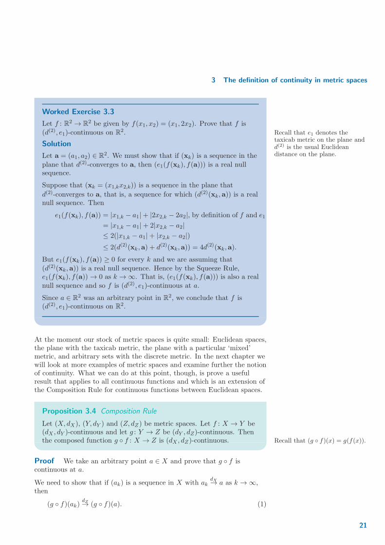
Worked Exercise 3.3

Let f : R2 → R2 be given by f(x1, x2) = (x1, 2x2). Prove that f is

(d(2), e1)-continuous on R2. Recall that e1 denotes the

taxicab metric on the plane andd(2) is the usual Euclideandistance on the plane.

Solution

Let a = (a1, a2) ∈ R2. We must show that if (xk) is a sequence in the

plane that d(2)-converges to a, then (e1(f(xk), f(a))) is a real nullsequence.

Suppose that (xk = (x1,kx2,k)) is a sequence in the plane that

d(2)-converges to a, that is, a sequence for which (d(2)(xk,a)) is a realnull sequence. Then

e1(f(xk), f(a)) = |x1,k − a1|+ |2x2,k − 2a2|, by definition of f and e1

= |x1,k − a1|+ 2|x2,k − a2|≤ 2(|x1,k − a1|+ |x2,k − a2|)≤ 2(d(2)(xk,a) + d(2)(xk,a)) = 4d(2)(xk,a).

But e1(f(xk), f(a)) ≥ 0 for every k and we are assuming that

(d(2)(xk,a)) is a real null sequence. Hence by the Squeeze Rule,e1(f(xk), f(a)) → 0 as k → ∞. That is, (e1(f(xk), f(a))) is also a real

null sequence and so f is (d(2), e1)-continuous at a.

Since a ∈ R2 was an arbitrary point in R

2, we conclude that f is(d(2), e1)-continuous on R

2.

At the moment our stock of metric spaces is quite small: Euclidean spaces,the plane with the taxicab metric, the plane with a particular ‘mixed’metric, and arbitrary sets with the discrete metric. In the next chapter wewill look at more examples of metric spaces and examine further the notionof continuity. What we can do at this point, though, is prove a usefulresult that applies to all continuous functions and which is an extension ofthe Composition Rule for continuous functions between Euclidean spaces.

Proposition 3.4 Composition Rule

Let (X, dX), (Y, dY ) and (Z, dZ ) be metric spaces. Let f : X → Y be(dX , dY )-continuous and let g : Y → Z be (dY , dZ)-continuous. Thenthe composed function g ◦ f : X → Z is (dX , dZ)-continuous. Recall that (g ◦ f)(x) = g(f(x)).

Proof We take an arbitrary point a ∈ X and prove that g ◦ f iscontinuous at a.

We need to show that if (ak) is a sequence in X with akdX→ a as k → ∞,

then

(g ◦ f)(ak) dZ→ (g ◦ f)(a). (1)

21


Write yk = f(ak) and y = f(a). Since f is (dX , dY )-continuous on X, weknow that

yk = f(ak)dY→ f(a) = y as k → ∞.

That is, the sequence (dY (yk, y)) is a real null sequence.

But the function g is (dY , dZ)-continuous on Y and so it follows by thedefinition of continuity for g that

g(yk)dZ→ g(y) as k → ∞.

This means that equation (1) holds, because g(yk) = (g ◦ f)(ak) andg(y) = (g ◦ f)(a).Thus g ◦ f is continuous at the arbitrary point a ∈ X, and so we concludethat g ◦ f is continuous on X.

Exercise 3.1

Let (X, d) and (Y, e) be metric spaces, and let b ∈ Y be fixed. Supposethat f : X → Y is (d, e)-continuous on X.

Use the Reverse Triangle Inequality to prove that g : X → R given byg(x) = e(f(x), b) is (d, d(1))-continuous on X.

22



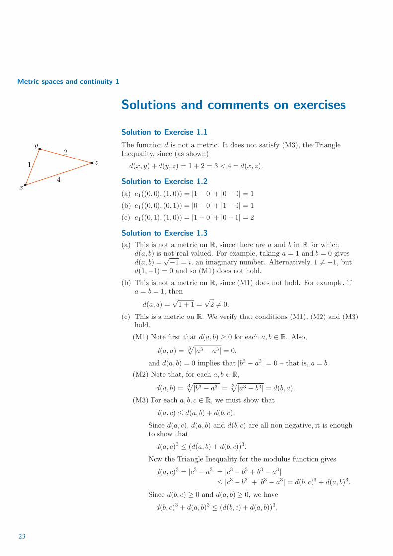
Solution to Exercise 1.1

The function d is not a metric. It does not satisfy (M3), the TriangleInequality, since (as shown)

x

1

y

4

z

2

d(x, y) + d(y, z) = 1 + 2 = 3 < 4 = d(x, z).


(a) e1((0, 0), (1, 0)) = |1− 0|+ |0 − 0| = 1

(b) e1((0, 0), (0, 1)) = |0− 0|+ |1 − 0| = 1

(c) e1((0, 1), (1, 0)) = |1− 0|+ |0 − 1| = 2


(a) This is not a metric on R, since there are a and b in R for whichd(a, b) is not real-valued. For example, taking a = 1 and b = 0 givesd(a, b) =

√−1 = i, an imaginary number. Alternatively, 1 6= −1, but

d(1,−1) = 0 and so (M1) does not hold.

(b) This is not a metric on R, since (M1) does not hold. For example, ifa = b = 1, then

d(a, a) =√1 + 1 =

√2 6= 0.

(c) This is a metric on R. We verify that conditions (M1), (M2) and (M3)hold.

(M1) Note first that d(a, b) ≥ 0 for each a, b ∈ R. Also,

d(a, a) = 3√

|a3 − a3| = 0,

and d(a, b) = 0 implies that |b3 − a3| = 0 – that is, a = b.

(M2) Note that, for each a, b ∈ R,

d(a, b) = 3√

|b3 − a3| = 3√

|a3 − b3| = d(b, a).

(M3) For each a, b, c ∈ R, we must show that

d(a, c) ≤ d(a, b) + d(b, c).

Since d(a, c), d(a, b) and d(b, c) are all non-negative, it is enoughto show that

d(a, c)3 ≤ (d(a, b) + d(b, c))3.

Now the Triangle Inequality for the modulus function gives

d(a, c)3 = |c3 − a3| = |c3 − b3 + b3 − a3|≤ |c3 − b3|+ |b3 − a3| = d(b, c)3 + d(a, b)3.

Since d(b, c) ≥ 0 and d(a, b) ≥ 0, we have

d(b, c)3 + d(a, b)3 ≤ (d(b, c) + d(a, b))3,

23


and so

d(a, c)3 ≤ (d(b, c) + d(a, b))3 = (d(a, b) + d(b, c))3,

as required.

Hence (M1)–(M3) hold and we conclude that d is a metric for R.


It is certainly the case that d(a,b) is always non-negative and for eacha ∈ R

2, d(a,a) = 0.

Now suppose that a = (a1, a2),b = (b1, b2) ∈ R2 with d(a,b) = 0. We

must show that a = b.

If d(a,b) = 0, then |b1 − a1|+ d0(a2, b2) = 0, which, since both | · | and d0are always non-negative, implies

|b1 − a1| = 0 and d0(a2, b2) = 0.

Hence, since | · | and d0 are metrics on R (and so satisfy (M1)), botha1 = b1 and a2 = b2. Thus a = b as required.


We need to show that for any choice of a = (a1, a2),b = (b1, b2) ∈ R2, we

have d(a,b) = d(b,a). This follows directly from the correspondingproperties of | · | and d0 when considered as metrics on R:

d(a,b) = |b1 − a1|+ d0(a2, b2)

= |a1 − b1|+ d0(b2, a2), by (M2) for | · | and d0

= d(b,a),

as required.


Let a ∈ X and suppose that r ≥ 0.

Since Bd0[a, r] = {x ∈ X : d0(a, x) ≤ r} and d0(a, x) = 1 unless a = x


Bd0[a, r] =

{

{a}, if 0 ≤ r < 1,X, if r ≥ 1.


Let a ∈ X and suppose that r > 0.

Since Sd0(a, r) = {x ∈ X : d0(a, x) = r} and d0(a, x) = 1 unless a = x


Sd0(a, r) =

{a}, if r = 0,X − {a}, if r = 1,∅, otherwise.

24



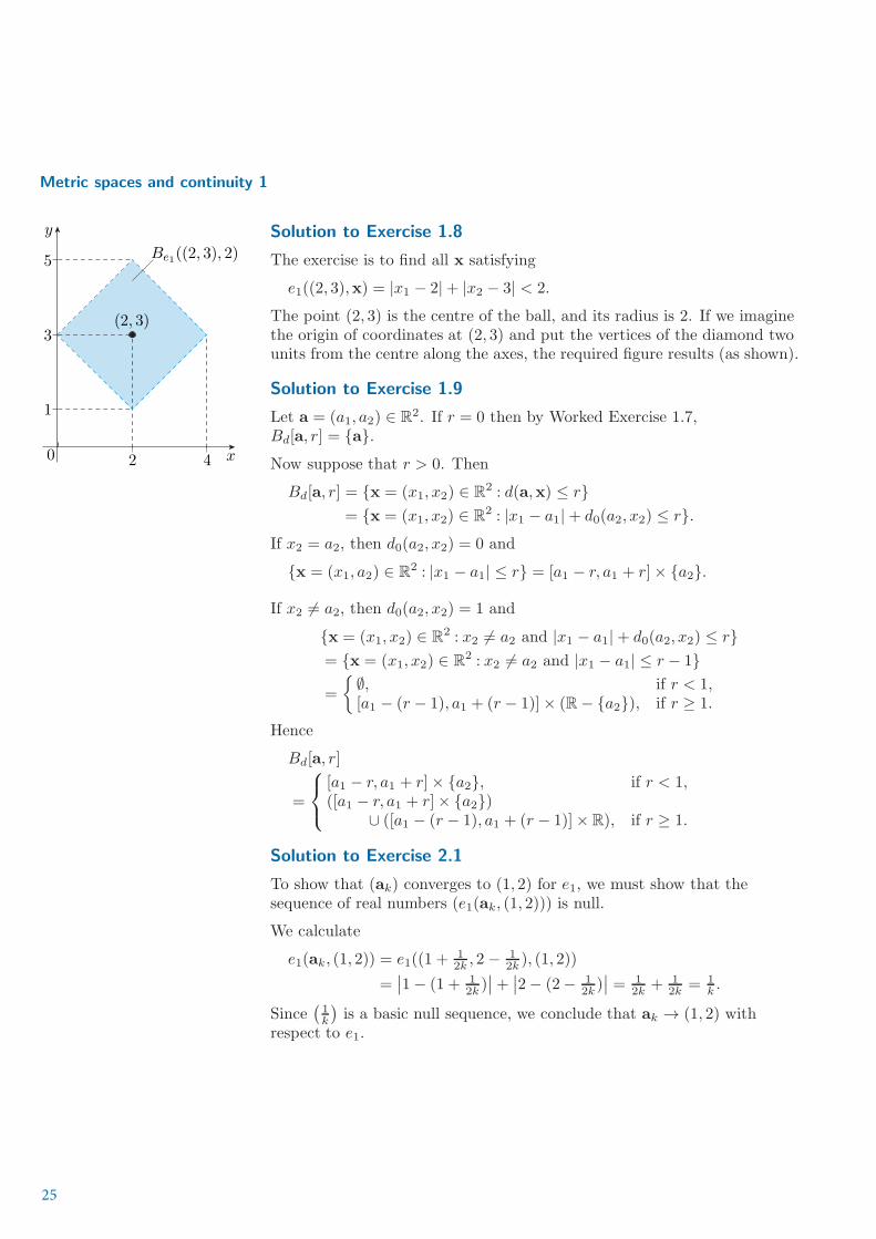
The exercise is to find all x satisfying

e1((2, 3),x) = |x1 − 2|+ |x2 − 3| < 2.

The point (2, 3) is the centre of the ball, and its radius is 2. If we imaginethe origin of coordinates at (2, 3) and put the vertices of the diamond twounits from the centre along the axes, the required figure results (as shown).

Be1((2, 3), 2)

0 2 4 x

1

3

5

y

(2, 3)


Let a = (a1, a2) ∈ R2. If r = 0 then by Worked Exercise 1.7,

Bd[a, r] = {a}.Now suppose that r > 0. Then

Bd[a, r] = {x = (x1, x2) ∈ R2 : d(a,x) ≤ r}

= {x = (x1, x2) ∈ R2 : |x1 − a1|+ d0(a2, x2) ≤ r}.

If x2 = a2, then d0(a2, x2) = 0 and

{x = (x1, a2) ∈ R2 : |x1 − a1| ≤ r} = [a1 − r, a1 + r]× {a2}.

If x2 6= a2, then d0(a2, x2) = 1 and

{x = (x1, x2) ∈ R2 : x2 6= a2 and |x1 − a1|+ d0(a2, x2) ≤ r}

= {x = (x1, x2) ∈ R2 : x2 6= a2 and |x1 − a1| ≤ r − 1}

=

{

∅, if r < 1,[a1 − (r − 1), a1 + (r − 1)]× (R− {a2}), if r ≥ 1.

Hence

Bd[a, r]

=

[a1 − r, a1 + r]× {a2}, if r < 1,([a1 − r, a1 + r]× {a2})

∪ ([a1 − (r − 1), a1 + (r − 1)]× R), if r ≥ 1.


To show that (ak) converges to (1, 2) for e1, we must show that thesequence of real numbers (e1(ak, (1, 2))) is null.

We calculate

e1(ak, (1, 2)) = e1((1 +12k , 2 − 1

2k ), (1, 2))

=∣

∣1− (1 + 12k)∣

∣+∣

∣2− (2− 12k)∣

∣ = 12k

+ 12k

= 1k.

Since(

1k

)

is a basic null sequence, we conclude that ak → (1, 2) withrespect to e1.

25



Let (ak) be a sequence in X and suppose that it converges (in d0) toa ∈ X.

Then, by the definition of convergence, it must be the case that (d0(ak, a))is a real null sequence and so, in particular, there is N ∈ N such that fork > N , |d0(ak, a)| < 1.

But d0(ak, a) can only equal 1 or 0, so this means that there must beN ∈ N such that for k > N , d0(ak, a) = 0. Since d0 is a metric on X,property (M1) tells us that for k > N , ak = a. In other words, thesequence (ak) is eventually constant, as required.


We take a general point a ∈ X and prove that g is (d, d(1))-continuous at

a. To do this, we take a sequence (xk) in X with xk

d→ a as k → ∞ and

show that g(xk)d(1)

→ g(a). This means we must show that

d(1)(g(xk), g(a)) → 0 as k → ∞,

and so we find an upper bound for this quantity.

Using the definition of g, and the Reverse Triangle Inequality for e, wefind that

d(1)(g(xk), g(a)) = |g(xk)− g(a)|= |e(f(xk), b)− e(f(a), b)|≤ e(f(xk), f(a)). (2)

Since f is (d, e)-continuous on X and xk

d→ a as k → ∞, we have that

f(xk)e→ f(a).

So (e(f(xk), f(a))) is a null sequence. Hence, applying the Squeeze Ruleto (2) shows that

(

d(1)(g(xk), g(a)))

is also a null sequence. That is,

(g(xk)) converges to g(a) for d(1). Thus g is (d, d(1))-continuous at a.

Since the choice of a is arbitrary, g is (d, d(1))-continuous on X.

26

Index

Index

Bd(a, r), the open ball of radius r with centre a, 11Bd[a, r], the closed ball of radius r with centre a, 11balls

closed, 11open, 11

centre, 11closed ball, 11Composition Rule

for continuous functions between metric spaces, 20continuity at a point

for metric spaces, 19continuity for metric spaces, 19continuous function

between metric spaces, 19continuous functions between metric spaces

Composition Rule, 20convergent sequence

in a metric space, 16

d-closed ball, 11definition

d-convergent sequence, 16d-divergent sequence, 16closed ball, 11continuous function between metric spaces, 19convergent sequence in a metric space, 16discontinuous function between metric spaces, 19eventually constant, 17metric space, 5open ball, 11sequence in a metric space, 15sphere, 11

discontinuous functionbetween metric spaces, 19

discrete metric, 6distance

in a metric space, 5distance function, 4d-open ball, 11d-sphere, 11divergence, 16divergent sequence

in a metric space, 16

Euclidean metric, 5

Euclidean distance function, 4Euclidean n-space, 5eventually constant, 17

function(d, e)-continuous, 19(d, e)-discontinuous, 19

limit of a sequence, 16

metric, 4, 5discrete, 6Euclidean, 5mixed (on the plane), 10taxicab, 8, 13

metric space, 5points, 5Reverse Triangle Inequality, 6

mixed metric in the plane, 10

open ball, 11

point in a metric space, 5

radius, 11Reverse Triangle Inequality

for metrics, 6

Sd(a, r), the sphere of radius r with centre a, 11sequence

eventually constant, 17sequence in a metric space, 15

convergence, 16divergence, 16limit, 16

sphere, 11

taxicab metric, 8open balls, 12

Triangle Inequalitycondition for metrics, 5in R

n, 4

unit closed ball, 11unit open ball, 11unit sphere, 11

27

Metric spaces and continuity - The Open University

Documents

Transcript of Metric spaces and continuity - The Open University