HAL Id: hal-01333696https://hal.archives-ouvertes.fr/hal-01333696

Submitted on 18 Jun 2016

HAL is a multi-disciplinary open accessarchive for the deposit and dissemination of sci-entific research documents, whether they are pub-lished or not. The documents may come fromteaching and research institutions in France orabroad, or from public or private research centers.

L’archive ouverte pluridisciplinaire HAL, estdestinée au dépôt et à la diffusion de documentsscientifiques de niveau recherche, publiés ou non,émanant des établissements d’enseignement et derecherche français ou étrangers, des laboratoirespublics ou privés.

Dynamics of unsymmetric piecewise-linear/non-linearsystems using finite elements in time

Yu Wang

To cite this version:Yu Wang. Dynamics of unsymmetric piecewise-linear/non-linear systems using finite elements in time.Journal of Sound and Vibration, Elsevier, 1995, �10.1006/jsvi.1994.0369�. �hal-01333696�

DYNAMICS OF UNSYMMETRICPIECEWISE-LINEAR/NON-LINEAR SYSTEMS

USING FINITE ELEMENTS IN TIME

Yu Wang

Department of Mechanical Engineering, University of Maryland, 5401 Wilkens Avenue,Baltimore, Maryland 21228-5398, U.S.A.

The dynamic response and stability of a single-degree-of-freedom system withunsymmetric piecewise-linear/non-linear stiffness are analyzed using the finite elementmethod in the time domain. Based on a Hamilton’s weak principle, this method provides asimple and efficient approach for predicting all possible fundamental and sub-periodicresponses. The stability of the steady state response is determined by using Floquet’s theorywithout any special effort for calculating transition matrices. This method is applied to anumber of examples, demonstrating its effectiveness even for a strongly non-linear probleminvolving both clearance and continuous stiffness non-linearities. Close agreement is foundbetween available published findings and the predictions of the finite element in timeapproach, which appears to be an efficient and reliable alternative technique for non-lineardynamic response and stability analysis of periodic systems.

1. INTRODUCTION

In a large class of vibrating systems there exist piecewise-linear or piecewise-non-linear

stiffnesses, due to the presence of gaps, clearances, backlash and impacting components.

Bearings, gears, impact print hammers and offshore structures are a few examples that fall

into this category. In the design of these systems, it is essential to obtain a comprehensive

understanding of their dynamic behavior in order to prevent excessive levels of noise and

vibration. For a simple piecewise-linear system, its dynamic response may be solved exactly

because the exact solution form is known in the intervals which the system possesses constant

stiffness characteristics [1, 2]. However, the characteristics of a general system are inherently

non-linear and the prediction of its response is not an easy task, particularly if the stiffness

is piecewise-non-linear.In this paper a numerical study is presented of unsymmetric piecewise-linear/non-linear

systems subject to general periodic excitations. Such systems are often used as models of

compliant offshore structures and articulated mooring towers [3] and their dynamics have

been previously investigated with well-illustrated complex characteristics in their response,

including chaotic vibrations. A common solution procedure for the strongly non-linear

system is the numerical time integration, which can give both transient and steady state

solutions. However, there are some difficulties in this approach. For example, it is usually

very time-consuming to obtain the system response with respect to a system parameter or

parameters, especially in parameter regions where multi-valued responses exist.

Furthermore, numerical integration with digital computers may encounter numerical

difficulties for some types of integration algorithms, particularly when the non-linearity

becomes very strong [4, 5].

An alternative approach is the harmonic balance method. With assumed waveforms of

vibration, approximate solutions for a single degree-of-freedom oscillator are determined

in reference [6]. A more general harmonic balance procedure is developed in references [7–9]

and has been applied to the two different unsymmetric piecewise-linear systems given in

references [3] and [6]. The approach is known to be limited by its ability of solving the

resulting non-linear algebraic equations. For a number of different implementations of the

procedure [10–13], it is found that the strength of non-linearity, the number of harmonics

sought in the solution and the relative magnitudes of higher harmonics with respect to the

fundamental are, among others, the major factors that are instrumental for the success of

the method [11, 13]. In particular, if an impulse-like force, for example, generated by a rigid

stop, is applied to the system, a large number of higher harmonics are inevitably required,

giving rise to a large number of system equations. In this case, it is usually difficult to achieve

convergence in the numerical solution.

Another possible approach is the use of the finite element in time method (FET) based

on Hamilton’s principle [14–17], in which the solution for all the spatial degrees of freedom

at all time steps within a given time interval of interest is sought via a set of algebraic

equations. Some recent development has shown that this approach offers several potential

advantages over numerical solution of ordinary differential equations in the time domain,

including the flexibility in formulating the problem directly from system energy expressions,

the greater accuracy at specific time points of interest, and the use of adaptive finite elements

to improve computational efficiency and accuracy [14, 17–19].

For obtaining the periodic response of the piecewise-linear/non-linear system,

moreover, two specific features of the finite elements in time make the approach an ideal

tool. First, the periodic solution can be made readily available by assembling a number

of time elements and imposing the appropriate periodic boundary constraint relations, in

contrast with time-stepping methods, which require initial conditions to start the

integration procedure but cannot impose periodic boundary conditions. For a harmonic

balance procedure, the periodicity condition of a solution is attained by the periodic

functions in Fourier series expansions. For the time finite element method, there is no

such restriction imposed on the interpolation functions and the conventional shape

functions can be used. In fact, it is easy to show that the Fourier series approach is a

special case of finite elements in time in which harmonics are used as trial and shape

functions for a single time element [19].

The second advantageous feature is the straightforward determination of stability of the

periodic solution. Since the corresponding transition matrix for the analysis of stability of

small perturbations about the periodic solution is a by-product of the FET procedure,

Floquet’s stability theory can be readily applied without any special effort.

These unique characteristics of the FET method have created a wide range of interest in

the field of dynamics and control, where it has been successfully used for analysis and design

of analytic-non-linear rotorcraft systems [14–16, 19], for dynamics of multi-body systems

[17, 20] and for optimal control [21]. It appears that the method is well-suited as an efficient

and consistent approach to predicting the dynamic response of piecewise-linear/non-linear

systems. The focus of this paper is to apply the FET method to the unsymmetric

piecewise-linear (and -non-linear) systems in order to demonstrate its effectiveness. The first

objective of this investigation is to develop the solution of the equation of motion for

piecewise-linear/non-linear systems with finite elements in time. Next, a number of

techniques for efficient numerical calculations and parametric studies are presented. Finally,

the predictions of this method, when applied to several piecewise linear and non-linear

problems, are discussed. The stability of the periodic solution is analyzed using Floquet’s

theory.

2. EQUATION OF MOTION

The response of the system analyzed in the present investigation is described by a

non-linear equation of motion, expressed in the form

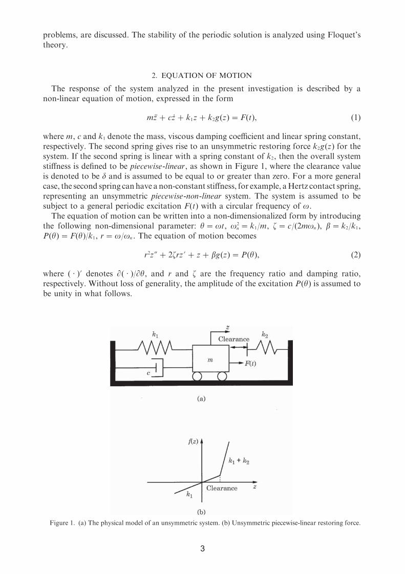
mz+ cz+ k1z+ k2g(z)=F(t), (1)

where m, c and k1 denote the mass, viscous damping coefficient and linear spring constant,

respectively. The second spring gives rise to an unsymmetric restoring force k2g(z) for the

system. If the second spring is linear with a spring constant of k2, then the overall system

stiffness is defined to be piecewise-linear, as shown in Figure 1, where the clearance value

is denoted to be � and is assumed to be equal to or greater than zero. For a more general

case, the second spring canhave a non-constant stiffness, for example, aHertz contact spring,

representing an unsymmetric piecewise-non-linear system. The system is assumed to be

subject to a general periodic excitation F(t) with a circular frequency of �.

The equation of motion can be written into a non-dimensionalized form by introducing

the following non-dimensional parameter: �=�t, �2n = k1/m, �= c/(2m�n ), �= k2/k1,

P(�)=F(�)/k1, r=�/�n . The equation of motion becomes

r2z�+2�rz'+ z+ �g(z)=P(�), (2)

where ( · )' denotes �( · )/��, and r and � are the frequency ratio and damping ratio,

respectively. Without loss of generality, the amplitude of the excitation P(�) is assumed to

be unity in what follows.

Figure 1. (a) The physical model of an unsymmetric system. (b) Unsymmetric piecewise-linear restoring force.

3. FINITE ELEMENT METHOD IN THE TIME DOMAIN

The finite element method in the time domain for obtaining solutions to dynamics

problems is based on a weak form of Hamilton’s law of varying action [14, 18]. The

commonly known as Hamilton’s weak principle can be expressed in its general displacement

form as

�tF

tI

(�L+ �W) dt= �z · p�tFtI , (3)

which describes the real motion of the system between the two known times tI and tF . Here,

L and W denote the Lagrangian and the work done by the generalized forces of the system,

respectively, and p= �L/�z is the set of the generalized momenta. For the

piecewise-linear/non-linear system described by equation (2), the variational equation

becomes

��F

�I

{�z' · (r2z')+ �z · [−2�rz'− z− �g(z)]+ �z · P(�)} d�= �z · p��F�I. (4)

Here, p= r2z' and the time interval of interest, T= �F − �I , equals the period of steady state

response of the system. For example, T=2� for the fundamental periodic response of a

harmonic excitation.

In this variational equation, z and �z are simply required to be continuous, and p appears

only as a discrete quantity at the ends of the time interval. These boundary terms are strictly

enforced as natural boundary conditions, allowing p to be determined without

differentiation of z [14, 17, 18]. Because of these special features, the use of the finite element

method is the most powerful tool for an easy approximation of equation (4).

In a finite element approximation to the dynamic equation (4), the time interval T is

divided into a finite number (Ne ) of time elements, usually equally spaced for convenience.

Similar to the standard finite element technique in spatial discretization, a set of nodal

displacements Zi for each time element i are defined, and the displacement z and velocity

z' within the element are interpolated among the nodal displacements Zi by using standard

shape functions, for example, the Lagrange’s polynomials, as

z(�)=Ni ()Zi and z'(�)=N'i ()Zi , =(�− �i )/(�i+1 − �i ), i=1, 2, . . . , Ne ,

(5, 6)

where the vector N for the elemental shape function has (k+1) components of polynomial

function if the order of interpolation is chosen to be k. Correspondingly, the nodal

displacement vector Zi has (k+1) temporal components for the time element. The Lagrange

family of interpolation functions is used in this study. Thus the equation of motion (4) can

be put in the following variational form for time element i:

��i+1

�i

{�ZTi [N'Ti r2N'i Zi −2�NT

i rN'i NiZi − �NTi g(z)]+ �ZT

i NTi P(�)} d�= �ZT

i Bi , (7)

where Bi is a vector of (k+1) elements containing linear momenta of the dynamic system

at the two ends of the time element,Bi = {−p(�i ), 0, . . . , 0, p(�i+1)}T. Since �Zi is completely

arbitrary, the finite element approximation at the element level is given by

AiZi +Gi (Zi )+Pi =Bi , (8)

where

Ai =��i+1

�i

N'Ti r2N'i d�−2� ��i+1

�i

NTi rN'i d�−�

�i+1

�i

NTi Ni d�, (9)

Gi =−� ��i+1

�i

NTi g(z) d�, Pi =�

�i+1

�i

NTi P(�) d�. (10, 11)

The variational equation (4) can now be represented by finite element approximation

equations that correspond to the nodal point displacements of the assemblage of finite

elements, as a sum of integrations over the time intervals of all time elements. Furthermore,

for periodic steady state response, the momentum vector vanishes since the periodic

boundary condition requires both displacements and velocities to be identical at �1 and �Ne +1,

or z(�1)= z(�Ne +1) and p(�1)= p(�Ne +1). Therefore, the dynamic response is described at the

system level by

AZ+G(Z)+P= 0, (12)

where, with a summation notation representing the element assemblage operation,

Z= �Ne

i=1

Zi , (13)

A= �Ne

i=1

Ai = �Ne

i=1 ���i+1

�i

N'Ti r2N'i d�−2� ��i+1

�i

NTi rN'i d�−�

�i+1

�i

NTi Ni d��, (14)

G= �Ne

i=1

Gi =−� �Ne

i=1 ��i+1

�i

NTi g(z) d�, (15)

O= �Ne

i=1

Pi = �Ne

i=1 ��i+1

�i

NTi P(�) d�. (16)

Thus, the finite element approximation results in a set of non-linear algebraic equations in

Ne unknown nodal displacement vectors.

In view of a numerical solution method—for example, the Newton–Raphson method—it

is often necessary to derive a linear approximation of equation (12). For a given state of

vibration Z(n) in an iteration solution procedure, a neighboring state can be expressed by

adding an increment,

Z(n+1) =Z(n) +Z(n). (17)

For a small increment, the non-linear equation (12) can be expanded into a set of Taylor

series, and a set of linear incremental equations are obtained by retaining only the linear

terms in the expansions, in the form

H(n) +K(n)Z(n) = 0, (18)

where

H(n) =A(n)Z(n) +G(n) +P, K(n) =A(n) + (�G/�Z)(n). (19, 20)

The matrix K is often referred to as the tangent matrix in finite element analysis. Equations

(17) and (18) represent an iteration process of the Newton–Raphson method, from which

the steady state response Z can be calculated. For a converged solution, Z(n) becomes nearly

zero.

It should be pointed out that the linearization procedure can be performed either on the

variational equation (4) of Hamilton’s weak principle or after the finite element

approximation. Conceptually, these linear approximations to the non-linear algebraic

system are equivalent, although they may yield different implications in the formulation of

analytical equations and in numerical computation. This issue is similar to that involved in

different implementations of the harmonic balance method [22]. For the one-degree-of-free-

dom problem considered in this investigation, all formulae are worked out in explicit forms,

regardless of the stage of linearization. Furthermore, for unsymmetric piecewise-linear

systems, the formulation can be greatly simplified by explicit expressions for the integrals

involving the restoring force of the second spring. In addition, for a general parametric study,

one can use various numerical procedures to obtain the solution of the nonlinear algebraic

equations (12) for a variable parameter. For example, a bifurcation diagram of the

unsymmetric piecewise-linear system with variation of stiffness ratio � can be easily traced

by first seeking the solution for a small value of � of weak non-linearity and then increasing

the parameter and obtaining the corresponding solution with a predictor–corrector method.

These are the subjects of the following section on numerical calculations.

4. NUMERICAL CALCULATIONS

4.1. evaluation of integrals

Calculation of the solution of the non-linear equation (12) or the linearized equation (18)

requires evaluation of the integrals of each time element in matrix A and vectors G and Pin equations (14)–(16). The integral components of matrix A and vector P are constants and,

therefore, they need to be calculated only once. In addition, if identical interpolation

functions are used for different time elements, the corresponding integrals are identical. With

polynomial interpolation functions (e.g., Lagrangian polynomials), each integral

component of the matrix A can be made exact analytically without quadrature

approximation.

The evaluation of the elements of vector G and matrix �G/�Z,

Gi =−� ��i+1

�i

NTi g(z) d�, (21)

�Gi /�Zj =−� ��i+1

�i

NTi �g(z)/�zNj d� (i, j=1, 2, . . . , Ne ), (22)

requires a knowledge of the zeros of the function (z(�)− �) with the interval [�i , �i+1]. Since

the displacement z within the interval is interpolated by polynomials among the temporal

nodes Zi , these zeros are the roots of a polynomial and therefore can be easily determined

in numerical computation of a computer program. Given the m roots, 1, 2, . . . , m , and

the sign of function (z− �), s1, s2, . . . , sm+1, corresponding to the intervals

[0, 1], [1, 2], . . . , [m , m+1] with 0 = �i and m+1 = �i+1, the integrals (21) and (22) are

expressed, respectively, as a sum of integrals over the (m+ 1) intervals in the form

Gi =−� �m+1

k=1

hk �k

k−1

NTi g(z) d�, (23)

�Gi /�Zj =−� �m+1

k=1

hk �k

k−1

NTi �g(z)/�zNj d�. (24)

The corresponding step functions are given as

hk =�1 for sk � 0 (z� �),

0 for sk � 0 (z� �),(25)

For a piecewise-linear system, g(z)= h(z− �) and �g(z)/�z= h, with h to be the step

function defined above. The integrals (23) and (24) become definite integrals of polynomials

and, therefore, can be made exact analytically without numerical quadrature. Consequently,

this will increase efficiency of numerical computation for the solution. In addition, the

restoring force in the time interval of the ith element is determined only by the nodal

displacement Zi of the corresponding element. Therefore, �Gi /�Zj = 0 for j� i.

4.2. static condensation

The finite element method in the time domain has the crucial property that the dynamic

response of a system is sought through propagation forward in time. As a result, the resulting

tangent matrix K (20) is in a block-diagonal form and the set of linearized equations (18)

can be solved efficiently. The solution of equation (18) can be obtained without actually

assembling the global tangent matrix K and the residual vector H. This property is similar

to that of finite elements in space used in solid mechanics. There exists a standard procedure

of static condensation in the space finite element method, by which the elemental degrees

of freedom that are not involved in satisfying the inter-element compatibility are eliminated

before the element is assembled into the overall system equations, yielding fewer unknowns

in the system equations [23]. A similar procedure for finite elements in time is described in

reference [15] for obtaining the solution of linear equations (18) efficiently. It is briefly

discussed as follows.

Consider the tangent matrix K, the displacement and force vectors, Z and P, and the

boundary conditions B of linearized equation (18), to be partitioned as

�Kbb

Kib

Kbi

Kii��Zb

Zi�+�Hb

Hi�=�Bb

0 �, (26)

where b and i correspond the temporal nodes at the ends and in the interior of current time

element separately, andBb = {−p(�i ), p(�i+1)}T denotes the boundary conditions. The lower

part of equation (26) can be solved for Zi as

Zi =−K−1ii Hi −K−1

ii KibZb . (27)

When this equation is substituted into the upper part of equation (26) for Zi and the terms

are collected, the remaining equation for Zb can be written as

K� bbZb +H� b =Bb , (28)

where the reduced tangent matrix and force vector are given by

K� bb =Kbb −KbiK−1ii Kib , H� b =Hb −KbiK−1

ii Hi . (29, 30)

When the next element is generated, the condensation procedure can be applied identically,

resulting in a similar set of reduced equations. These two sets of reduced equations are further

condensed by imposing the compatibility conditions of the displacement vector and the

boundary conditions at the common node of the two elements, yielding the elimination of

the common node. The above procedure is repeated for each remaining element, and the

final set of equations is written as

�K� II

K� FI

K� IF

K� FF��ZI

ZF�+�H� I

H� F�=�BI

BF�, (31)

where I and F denote the initial and final time nodes, respectively, and BI =−pI =−p(�I )

and BF = pF = p(�F ). Finally, for the periodic steady state response it is required that

ZF =ZI and pI = pF . (32)

Therefore, the initial and final nodal displacements can be solved from equation (31) as

ZI =ZF =−(K� II +K� IF +K� FI +K� FF )−1(H� I +H� F ). (33)

This procedure is the same as Gaussian elimination. Once the boundary nodes have been

computed, then the condensed unknown nodes can be recovered by a back substitution

process for each corresponding condensation. The procedure is continued for all nodes in

the system, allowing a complete solution of the equations to be obtained.

4.3. parametric solution

The finite element in time method is ideally suited to parametric studies for obtaining

solution diagrams, since it can step from a known state of vibration to a neighboring state

corresponding to an incremental change in one of the governing parameters of the system.

The solution of the non-linear algebraic equations (12) with a variable parameter defines a

path in the corresponding state-parameter space, or the solution diagram. A method for

following the path is discussed next, which employs a predictor to move along a path

direction and a corrector to allow accurate path following.

Consider the solution diagram, defined by equation (12) as

F(Z, �)=A(�)Z+G(Z, �)+P= 0 (34)

for a variable parameter �, which can be the frequency ratio r, the stiffness ratio �, the

clearance value �, or any parameter of interest in the system. Define w to be the arc-length

along the solution path. Then, the derivative of equation (34) with respect to arc-length is

given as

�F�Z

dZdw

+�F��

d�

dw=0, (35)

where �F/�Z is the tangent matrix K defined in equation (18) by linearization. The above

derivative indicates where the path is going, allowing a step to be moved in that direction.

The arc-length is defined to be

�dZdw�

2

+d�

dw2

=1. (36)

Suppose that the current point on the path corresponds to a solution Z(n) and a parameter

value �(n): then, the next point farther along the path of step size h is defined as

Z(n+1) =Z(n) + hZ(n), �(n+1) = �(n) + h�(n), (37, 38)

where Z(n) and �(n) satisfy the derivative and unit arc-length equations (35) and (36); i.e.,

Z(n) =−�F�Z

−1�F��

(n)

�(n), �(n) =�1���F�Z

−1�F��

(n)

�2

+11/2

. (39, 40)

This procedure is known as the Euler predictor, which is of first order [24]. Higher order

predictors (e.g., Adams–Bashforth) are also available using higher derivatives of the solution

equation (34).

A predictor is essentially an approximation method. The predicted solution can

significantly drift off the solution path in one step or a sequence of predictor steps, and it

must be corrected to return more closely to the solution path [24]. The classical method is

a Newton–Raphson corrector with a sequence of iterations constrained to lie perpendicular

to the predictor direction and passing through predicted solution Z(n+1) and �(n+1). At

convergence, the corrector gives rise to an accurate solution.

Let Z(n+1) and �(n+1) be the corrector step from the current solution Z(n+1) and �(n+1),

satisfying the Newton–Raphson method such that

��F�Z

�F���

(n+1)

�Z��

(n+1)

=−F(n+1). (41)

The corrector direction is defined by

{ZT �}(n)�Z��

(n+1)

=0. (42)

On combining the above equations, the corrector step is the solution of the set of linear

equations

�(�F/�Z)(n+1)

Z(n)

(�F/��)(n+1)

�(n) ��Z��

(n+1)

=�−F(n+1)

0 �. (43)

The new value of the corrected point Z(n+2) and �(n+2) is given by

Z(n+2) =Z(n+1) +Z(n+1), �(n+2) = �(n+1) +�(n+1). (44, 45)

A finite number of corrector steps will be taken so that the norm of F is smaller than some

selected small number. Repetition of the above predictor and corrector process will follow

the solution path quite well, as shown in the numerical results presented in section 6.

5. STABILITY OF STEADY STATE SOLUTION

The stability of any periodic steady state solution obtained above is investigated by

considering small perturbations of the solution and the boundary condition in equation (31)

for the initial and final time nodes [15, 17]; hence, equations (31) becomes

�K� II

K� FI

K� IF

K� FF���ZI

�ZF�=�−�pI

�pF �. (46)

According to Floquet’s theory, the stability of the system is determined by the eigenvalues

of the transition matrix that relates the initial and final perturbations. This transition matrix

happens to be a by-product of the FET procedure, and is readily found by rearranging

equation (46):

��ZF

�pF �=� −K� −1IF K� II

K� FI −K� FFK� −1IF K� II

−K� −1IF

−K� −1IF K� FF���ZI

�pI �. (47)

Therefore, the same solution algorithm can be used for both the periodic response and

stability calculations. There is no need for a special effort in calculating the transition matrix,

as in, for example, references [25, 26]. This is useful in assessing the characteristics of the

non-linear system.

The stability of the steady state response is determined by the eigenvalues of the transition

matrix defined in equation (47). If the eigenvalue � with the larger modulus satisfies ���� 1,

then the periodic solution examined is asymptotically stable. When ���� 1, the solution is

unstable. Bifurcations occur if ���=1, resulting in qualitative changes in system dynamics

[27]. There are three types of bifurcations. The first type is a saddle-node bifurcation

corresponding to the merging of two periodic solutions. It occurs when �=1 and results

in the classical jump phenomena. The second type is a flip bifurcation associated with period

doubling of the response. It occurs when �=−1. Finally, if a pair of complex eigenvalues

have modulus one, the so-called Hopf bifurcation happens, resulting in an amplitude

modulated response of the system. For the system considered in this investigation, the first

two types of bifurcations are observed as discussed in the results presented in the next section.

It was previously shown that the Hopf bifurcation does not happen in a

single-degree-of-freedom system with piecewise-linear stiffness [2].

6. RESULTS

A simple unsymmetric bilinear system is considered first, in which �=0 and �=4. The

system is under a harmonic excitation P(�)= cos �. This system has been studied in

reference [3] using direct numerical integration and in references [7, 9] using the harmonic

balance method. The numerical results obtained by the finite element method are shown in

Figure 2, where the steady state amplitude is defined as half of the peak-to-peak of the

response. The frequency response is plotted as a function of the dimensionless frequency

ratio r, with damping ratio �=0·1. These results are found to agree very well with those

obtained by using direct integration and harmonic balance method.

The FET method yields all possible steady state solutions, including the sub-periodic and

the unstable solutions, for a wide range of frequency ratios. The order of the sub-periodic

vibration is denoted by m in the figure. A bifurcation from a stable solution on the

fundamental response to a stable solution on the sub-periodic of order 2 is found to occur

at r=2·27. The stability analysis reveals that it is a flip bifurcation. This bifurcation was

investigated in reference [3] by using a Poincare map. Numerical calculation of the transition

matrix in a harmonic balance analysis also showed the period doubling phenomena [9].

Resonant peaks of sub-periodic response appear regularly to the right of the fundamental

resonance with increasing order of sub-periodic vibration. Furthermore, to the left of the

fundamental resonance, the FET method shows a number of peaks occurring irregularly.

Figure 2. A frequency response plot for �=0, �=0·1 and �=4. ����, Stable; – – – –, unstable.

This behavior was also investigated in reference [3], where the correlation with the cyclic

moment of the Poincare point was shown.

The mth sub-periodic response is defined to have a period of oscillation equal to m times

the fundamental period, i.e., T=2m�, for the harmonic excitation. To obtain the

sub-periodic response without modifying the FET formulation, one simply takes the

excitation to be P(�)= cos m� and shifts the obtained solution with the frequency divided

by m.

To show the convergence of the obtained solutions and to find an adequate number of

time elements and an adequate order of interpolation functions, this problem has also been

computed with a different number of time elements and different order of Lagrangian

polynomials for the shape function. The results of the average amplitude obtained are listed

in Table 1. It is observed that the use of six time elements and quartic polynomials is sufficient

to obtain a well converged solution with three to four digit accuracy. Therefore, six time

elements and quartic polynomials are used for the numerical results shown hereafter. The

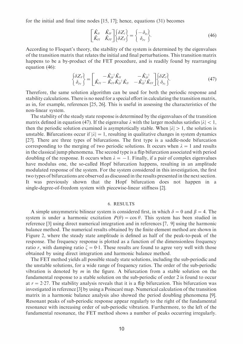
convergence development with subsequent iteration of the FET method for t=1·2 is shown

in Figure 3.

Table 1

Average amplitudes obtained with different numbers of time elements and different orders ofpolynomials

Order

�������������������������������Element 3 4 5 6

4 2·53389 2·52567 2·52664 2·526126 2·52333 2·52598 2·52601 2·525948 2·52479 2·52608 2·52594 2·52596

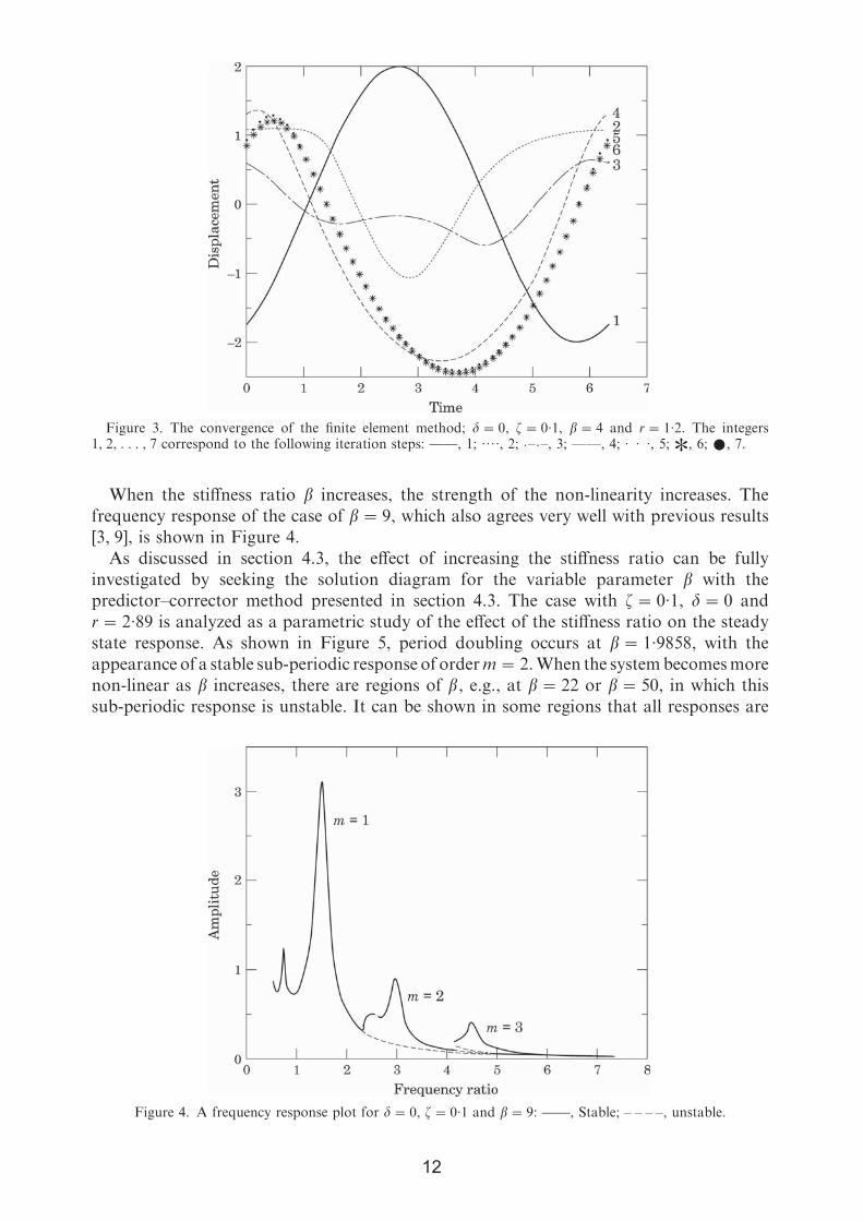
Figure 3. The convergence of the finite element method; �=0, �=0·1, �=4 and r=1·2. The integers1, 2, . . . , 7 correspond to the following iteration steps: ����, 1; ····, 2; ·–·–, 3; ——, 4; · · ·, 5; �, 6; �, 7.

When the stiffness ratio � increases, the strength of the non-linearity increases. The

frequency response of the case of �=9, which also agrees very well with previous results

[3, 9], is shown in Figure 4.

As discussed in section 4.3, the effect of increasing the stiffness ratio can be fully

investigated by seeking the solution diagram for the variable parameter � with the

predictor–corrector method presented in section 4.3. The case with �=0·1, �=0 and

r=2·89 is analyzed as a parametric study of the effect of the stiffness ratio on the steady

state response. As shown in Figure 5, period doubling occurs at �=1·9858, with the

appearance of a stable sub-periodic response of orderm=2.When the systembecomesmore

non-linear as � increases, there are regions of �, e.g., at �=22 or �=50, in which this

sub-periodic response is unstable. It can be shown in some regions that all responses are

Figure 4. A frequency response plot for �=0, �=0·1 and �=9: ����, Stable; – – – –, unstable.

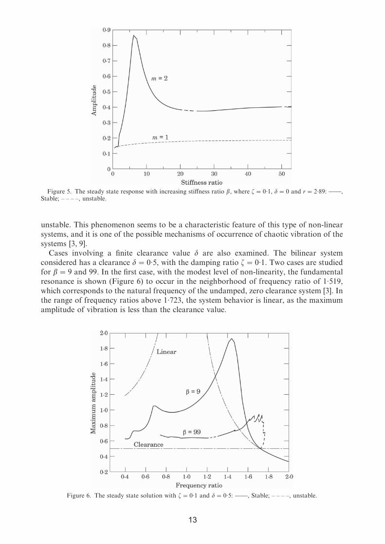
Figure 5. The steady state response with increasing stiffness ratio �, where �=0·1, �=0 and r=2·89: ����,Stable; – – – –, unstable.

unstable. This phenomenon seems to be a characteristic feature of this type of non-linear

systems, and it is one of the possible mechanisms of occurrence of chaotic vibration of the

systems [3, 9].

Cases involving a finite clearance value � are also examined. The bilinear system

considered has a clearance �=0·5, with the damping ratio �=0·1. Two cases are studied

for �=9 and 99. In the first case, with the modest level of non-linearity, the fundamental

resonance is shown (Figure 6) to occur in the neighborhood of frequency ratio of 1·519,

which corresponds to the natural frequency of the undamped, zero clearance system [3]. In

the range of frequency ratios above 1·723, the system behavior is linear, as the maximum

amplitude of vibration is less than the clearance value.

Figure 6. The steady state solution with �=0·1 and �=0·5: ����, Stable; – – – –, unstable.

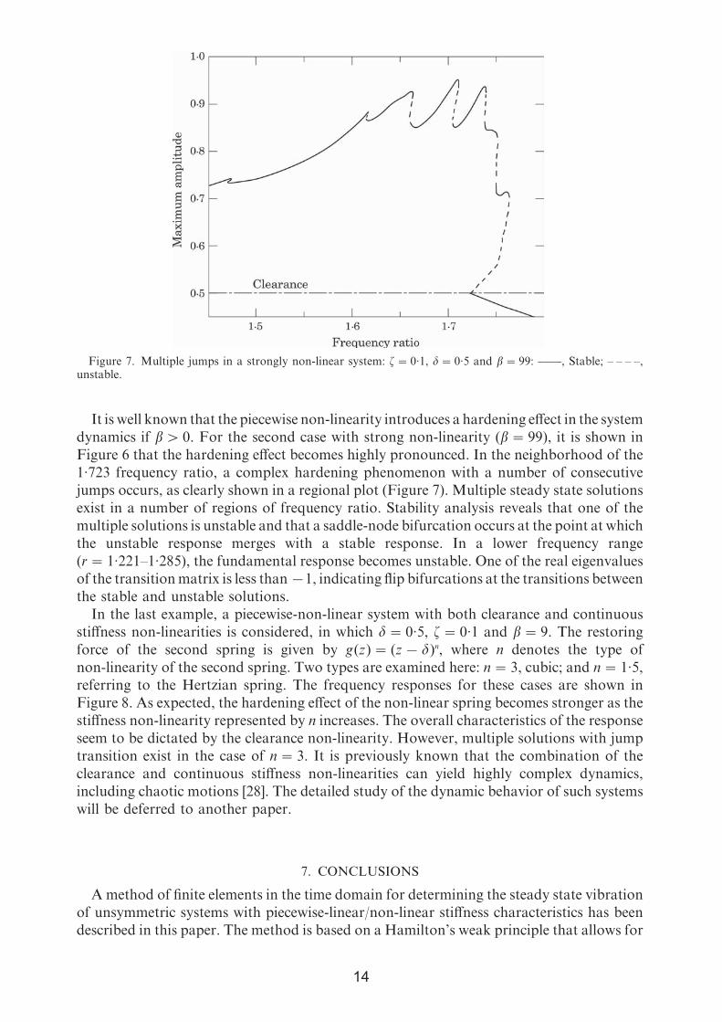
Figure 7. Multiple jumps in a strongly non-linear system: �=0·1, �=0·5 and �=99: ����, Stable; – – – –,unstable.

It is well known that the piecewise non-linearity introduces a hardening effect in the system

dynamics if �� 0. For the second case with strong non-linearity (�=99), it is shown in

Figure 6 that the hardening effect becomes highly pronounced. In the neighborhood of the

1·723 frequency ratio, a complex hardening phenomenon with a number of consecutive

jumps occurs, as clearly shown in a regional plot (Figure 7). Multiple steady state solutions

exist in a number of regions of frequency ratio. Stability analysis reveals that one of the

multiple solutions is unstable and that a saddle-node bifurcation occurs at the point at which

the unstable response merges with a stable response. In a lower frequency range

(r=1·221–1·285), the fundamental response becomes unstable. One of the real eigenvalues

of the transition matrix is less than −1, indicating flip bifurcations at the transitions between

the stable and unstable solutions.

In the last example, a piecewise-non-linear system with both clearance and continuous

stiffness non-linearities is considered, in which �=0·5, �=0·1 and �=9. The restoring

force of the second spring is given by g(z)= (z− �)n, where n denotes the type of

non-linearity of the second spring. Two types are examined here: n=3, cubic; and n=1·5,

referring to the Hertzian spring. The frequency responses for these cases are shown in

Figure 8. As expected, the hardening effect of the non-linear spring becomes stronger as the

stiffness non-linearity represented by n increases. The overall characteristics of the response

seem to be dictated by the clearance non-linearity. However, multiple solutions with jump

transition exist in the case of n=3. It is previously known that the combination of the

clearance and continuous stiffness non-linearities can yield highly complex dynamics,

including chaotic motions [28]. The detailed study of the dynamic behavior of such systems

will be deferred to another paper.

7. CONCLUSIONS

A method of finite elements in the time domain for determining the steady state vibration

of unsymmetric systems with piecewise-linear/non-linear stiffness characteristics has been

described in this paper. The method is based on a Hamilton’s weak principle that allows for

Figure 8. The response for both clearance and continuous stiffness non-linearities; �=0·1, �=0·5 and �=9:����, Stable; – – – –, unstable.

a simple choice of interpolation function and an easy problem formulation. The method

offers a number of special features that can be utilized for accurate numerical results with

only a few elements and for minimal computation effort. The stability of the steady state

solution is directly determined as the transition matrix of Floquet’s theory is readily

available.

This method is applied to unsymmetric piecewise-linear and piecewise-non-linear systems

and the numerical results are seen to provide excellent agreement with previous findings

of a direct numerical integration method and a harmonic balance method. Both stable and

unstable steady state solutions are determined. A parametric solution of the system

dynamics is performed with a predictor–corrector method. This possibility permits one to

investigate strongly non-linear systems with both clearance and continuous stiffness

non-linearities.

The finite element in time method has the flexibility for adaptive change of the order of

interpolation functions and the number of time elements. Therefore, the number of temporal

nodes can be easily changed from one iteration step to the next, as only the linearized

equations are assembled from each time element in each step. This fact may lead to a

systematic and effective impelementation for obtaining steady state solutions over a wide

range of system parameters and for obtaining solutions with greater accuracy at certain

specified time locations. This method is currently under development by the author in

applying the method to problems with discontinuities in the states and the state equations

(such as systems with pre-loaded springs and dry friction).

ACKNOWLEDGMENTS

This work is being carried out as part of a project supported by the National Science

Foundation under grant No. MSS-9308663, which is gratefully acknowledged. The author

would also like to than Professor Fred Tasker for his input as to the finite element in time

method.

REFERENCES

1. S. W. Shaw 1985 Journal of Applied Mechanics 52, 453–464. The dynamics of a harmonicallyexcited system having rigid amplitude constraints, part 1 and part 2.

2. S. Natsiavas 1990 Journal of Sound and Vibration 141, 97–102. Stability and bifurcation analysisfor oscillators with motion limiting constraints.

3. J. M. T. Thompson 1986 Nonlinear Dynamics and Chaos. New York: John Wiley.4. R. Singh, C. Padmanabhan and T. E. Rook 1992 In 22nd Biennial Mechanisms Conference,

Scottsdale, Arizona, ASME. Computation issues associated with gear rattle analysis.5. L. C. Lee 1993 Master’s thesis, Department of Mechanical Engineering, University of Maryland,

Baltimore. Numerical analysis of machine joints with clearances.6. S. Maezawa, H. Kumano and Y. Minakuchi 1980 Bulletin of the Japan Society of Mechanical

Engineers 23, 68–75. Forced vibrations in an unsymmetric piecewise-linear system excited bygeneral periodic force functions.

7. Y. S. Choi and S. T. Noah 1988 Journal of Sound and Vibration 121, 117–126. Force periodicvibration of unsymmetric piecewise-linear systems.

8. Y. B.Kim and S. T.Noah 1991 Journal ofAppliedMechanics 58, 545–553. Stability and bifurcationanalysis of oscillators with piecewise-linear characteristics: a general approach.

9. C. W. Wong, W. S. Zhang and S. L. Lau 1991 Journal of Sound and Vibration 149, 91–105.Periodic forced vibration of unsymmetrical piecewise-linear systems by incremental harmonicbalance method.

10. F. H. Ling and X. X. Wu 1987 International Journal of Non-linear Mechanics 22, 89–98.Fast Galerkin method and its application to determine periodic solutions of non-linear oscillators.

11. T. M. Cameron and J. H. Griffin 1989 Journal of Applied Mechanics 56, 149–154. An alternatingfrequency/time domain method for calculating the steady-state response of nonlinear dynamicsystems.

12. S. L. Lau, Y. K. Cheung and S. Y. Wu 1982 Transactions of the American Society of MechanicalEngineers, Journal of Applied Mechanics 49, 849–852. Variable parameter incrementation methodfor dynamic instability of linear and nonlinear systems.

13. C. Nataraj and H. D. Nelson 1989 Journal of Vibration, Acoustics, and Reliability in Design 111,187–193. Periodic solutions in rotor dynamic systems with nonlinear supports: a general approach.

14. M. Borri et al. 1985 Computers and Structures 20, 495–508. Dynamic response of mechanicalsystems by a weak Hamiltonian formulation.

15. M. Borri 1986 Computers and Mathematics with Applications 12A, 149–160. Helicopter rotordynamics by finite element time approximation.

16. O. A. Bauchau and C. H. Hong 1988 American Institute of Aeronautics and Astronautics Journal26, 1135–1142. Nonlinear response and stability analysis of beams using finite elements in time.

17. M. Borri, C. Bottasso and P. Mantegazza 1992 Meccanica 27, 119–130. Basic features of thetime finite element approach for dynamics.

18. D. A. Peters and A. P. Izadpanah 1988 Computational Mechanics 3, 73–88. Hp-version finiteelements for the space–time domain.

19. L.-J. Hou and D. A. Peters 1993 Mathematical Computation and Modeling 17, 29–46. Periodictrim solutions with hp-version finite elements in time.

20. F. J. Mello, M. Borri and S. N. Atluri 1990 Computers and Structures 37, 231–240. Time finiteelement methods for large rotational dynamics of multibody systems.

21. D. H. Hodges and R. R. Bless 1991 Journal of Guidance 14, 148–156. Weak Hamiltonian finiteelement method for optimal control problems.

22. A. A. Ferri 1986 Journal of Applied Mechanics 53, 455–456. On the equivalence of the incrementalharmonic balance method and the harmonic balance Newton–Raphson method.

23. K.-J. Bathe 1982 Finite Element Procedures in Engineering Analysis. Englewood Cliffs, NewJersey: Prentice-Hall.

24. W. I. Zangwill and C. B. Garcia 1981 Pathways to Solutions, Fixed Points, and Equilibria.Englewood Cliffs, New Jersey: Prentice-Hall.

25. C. S. Hsu 1977 Advances in Applied Mechanics 17, 245–301. On nonlinear parametric excitationproblems.

26. C. vonKerczek and S. H. Davis 1975 American Institute of Aeronautics and Astronautics Journal13, 1400–1403. Calculation of transition matrices.

27. J. Guckenheimer and P. Holmes 1983 Nonlinear Oscillations, Dynamical Systems, andBifurcations of Vector Fields. New York: Springer-Verlag.

28. A. Kahraman and R. Singh 1992 Journal of Sound and Vibration 151, 180–185. Dynamics of anoscillator with both clearance and continuous non-linearities.