Piecewise Affine Registration of Biological

Images for Volume Reconstruction

Alain Pitiot a,b,c,∗ Eric Bardinet b,d Paul M. Thompson c

Gregoire Malandain b

aMirada Solutions, Ltd., Level 1, 23-38 Hythe Bridge Street, Oxford, OX1 2EP,

United Kingdom 1

b EPIDAURE Laboratory, INRIA, Sophia Antipolis, France

cLaboratory of Neuro Imaging, UCLA School of Medicine, Los Angeles, USA

dCNRS, UPR640-LENA, Paris, France

Abstract

This manuscript tackles the reconstruction of 3D volumes via mono-modal reg-istration of series of 2D biological images (histological sections, autoradiographs,cryosections, etc.). The process of acquiring these images typically induces compos-ite transformations that we model as a number of rigid or affine local transformationsembedded in an elastic one. We propose a registration approach closely derived fromthis model.

Given a pair of input images, we first compute a dense similarity field betweenthem with a block matching algorithm. We use as a similarity measure an exten-sion of the classical correlation coefficient that improves the consistency of the field.A hierarchical clustering algorithm then automatically partitions the field into anumber of classes from which we extract independent pairs of sub-images. Our clus-tering algorithm relies on the Earth mover’s distribution metric and is additionallyguided by robust least-square estimation of the transformations associated witheach cluster. Finally, the pairs of sub-images are, independently, affinely registeredand a hybrid affine/non-linear interpolation scheme is used to compose the outputregistered image.

We investigate the behavior of our approach on several batches of histologicaldata and discuss its sensitivity to parameters and noise.

Key words: registration, clustering, reconstruction, histology, MRI

∗ Corresponding author.Email address: apitiot@loni.ucla.edu (Alain Pitiot).

1 Fax: +44 1865 265 501

Preprint submitted to Elsevier Science 26 January 2005

1 Introduction

A key component of medical image analysis, image registration essentiallyconsists of bringing two images, acquired from the same or different modali-ties, into spatial alignment. This process is motivated by the hope that moreinformation can be extracted from an adequate merging of these images thanfrom analyzing them independently. For instance, mono-modal registration ofa population’s MRIs can be used to build anatomical atlases (Collins et al.,2003; Thompson et al., 2000), while mono- or multi-modal registration of thesame patient’s data can help determine the nature of an anomaly (Jolesz et al.,2001) or monitor the evolution of a tumor (Haney et al., 2001) or other diseaseprocess (Rey et al., 2002).

In particular, pair-by-pair registration of a series of 2-D biological images(histological sections or autoradiographs) enables the reconstruction of a 3Dbiological image. Subsequent fusion with 3D data acquired from tomographicimaging modalities (e.g. MRI) then allows the tissue properties to be studiedin an adequate anatomic framework, using in vivo reference data.

More formally, given two input images, registering the floating (i.e., movable)image to the reference (i.e., fixed) one entails finding the transformation thatminimizes the dissimilarity between the transformed floating image and thereference. As such, it can be decomposed into three elements:

• a transformation space, which describes the set of admissible transforma-tions from which one is chosen to apply to the floating image;

• a similarity criterion, which measures the discrepancy between the images;and

• an optimization algorithm, which traverses the transformation space, insearch of the transformation that will minimize the similarity criterion.

A large variety of transformation spaces have been discussed in the literature:among others, one finds linear transformations (rigid, affine) and non-lineartransformations (polynomial (Woods et al., 1998), polyaffine (Feldmar and Ay-ache, 1996; Arsigny et al., 2003), elastic (Davatzikos, 1997; Gee et al., 1993) orfluid (Christensen, 1999)). Similarly, many similarity criteria have been pre-sented: Studholme et al. (1996) use normalized mutual information, Collinset al. (1995) cross-correlation, Roche et al. (2000) the correlation ratio, Ash-burner and Friston (1999) the squared intensity difference, etc. Optimizationalgorithms range from the straightforward Powell method (Collignon et al.,1995) to sophisticated multi-scale Levenberg-Marquardt techniques (Taubin,1993) or stochastic search (Wells et al., 1996) (please refer to Maintz andViergever (1998), van den Elsen et al. (1993) or Cachier (2002, Chapitre 1)

2

for thorough reviews of medical image registration).

1.1 Registration algorithms for 3-D reconstruction

By registering each pair of consecutive slices in the stack of biomedical images,we can recover a geometrically coherent 3-D alignment of the 2-D images. Thisproblem essentially consists of the mono-modal registration of similar objects(even though non-coherent distortions may occur between consecutive slices).A number of techniques have been proposed in the literature.

manual registration: Classically, people have relied on their anatomical ex-pertise to register images manually (Deverell et al., 1993; Rydmark et al.,1992), a time-consuming, operator-dependent and poorly reproducible pro-cess.

fiducial markers: The use of fiducial markers helps increase the reliability ofthe registration process (Ford-Holevinski et al., 1991; Goldszal et al., 1996,1995; Humm et al., 1995). In histology, physical markers (straight rigid nee-dles for instance) can be inserted into the organ to be processed, prior to theslicing step. They are later tracked in the images. A least square minimiza-tion process then attempts to recover the original geometrical configuration.

While obviously a lot less operator-independent and more reproduciblethan manual registration, the biases introduced by the non-orthogonalitybetween the needle’s axes and the cutting planes and the geometrical defor-mations undergone by the needle holes during the histological preparations(the chemical baths can collapse the holes) may significantly hamper theability of the least square minimization to recover the correct transforma-tion.

geometrical approaches: These require that feature elements be extracteda priori.: those elements are usually geometrically remarkable points suchas lines, curvature extrema or contours. Hibbard and Hawkins (1988) forinstance use principal axes to align digital autoradiograms. Better perfor-mances in terms of precision can be achieved by matching contours (Cohenet al., 1998; Zhao et al., 1993), edges (Kay et al., 1996; Kim et al., 1995) orpoints (Rangarajan et al., 1997).

While it could be argued that these techniques enable a better control overthe registration process, the segmentation of feature elements can sometimesbe as difficult a problem as the overall registration process itself, with similardrawbacks: non-reproducibility if the feature are extracted manually, lackof precision for fully automated segmentation, etc.

iconic approaches: They rely on the comparison of the intensities associ-ated to voxels in the input images. Usually, they can be casted into asimilarity-minimization framework where the transformation space is tra-versed in search for the transformation which minimizes the intensity dis-

3

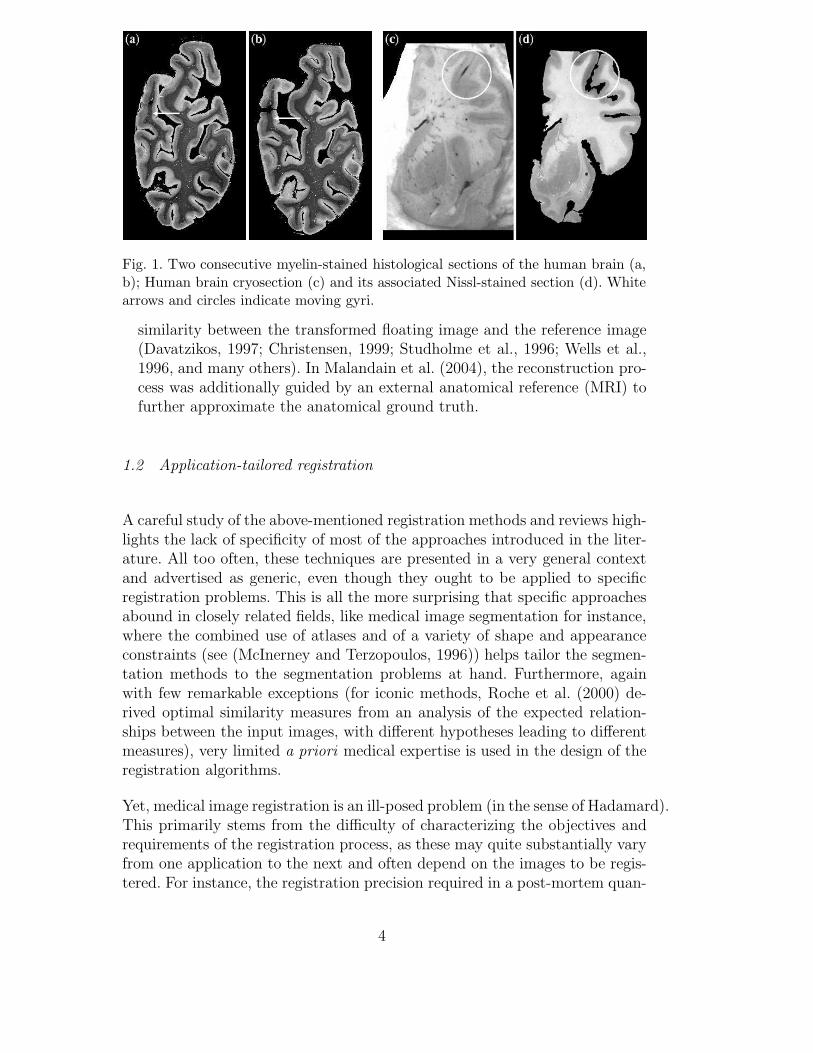
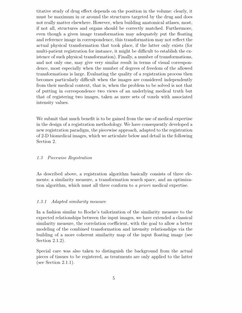
Fig. 1. Two consecutive myelin-stained histological sections of the human brain (a,b); Human brain cryosection (c) and its associated Nissl-stained section (d). Whitearrows and circles indicate moving gyri.

similarity between the transformed floating image and the reference image(Davatzikos, 1997; Christensen, 1999; Studholme et al., 1996; Wells et al.,1996, and many others). In Malandain et al. (2004), the reconstruction pro-cess was additionally guided by an external anatomical reference (MRI) tofurther approximate the anatomical ground truth.

1.2 Application-tailored registration

A careful study of the above-mentioned registration methods and reviews high-lights the lack of specificity of most of the approaches introduced in the liter-ature. All too often, these techniques are presented in a very general contextand advertised as generic, even though they ought to be applied to specificregistration problems. This is all the more surprising that specific approachesabound in closely related fields, like medical image segmentation for instance,where the combined use of atlases and of a variety of shape and appearanceconstraints (see (McInerney and Terzopoulos, 1996)) helps tailor the segmen-tation methods to the segmentation problems at hand. Furthermore, againwith few remarkable exceptions (for iconic methods, Roche et al. (2000) de-rived optimal similarity measures from an analysis of the expected relation-ships between the input images, with different hypotheses leading to differentmeasures), very limited a priori medical expertise is used in the design of theregistration algorithms.

Yet, medical image registration is an ill-posed problem (in the sense of Hadamard).This primarily stems from the difficulty of characterizing the objectives andrequirements of the registration process, as these may quite substantially varyfrom one application to the next and often depend on the images to be regis-tered. For instance, the registration precision required in a post-mortem quan-

4

titative study of drug effect depends on the position in the volume: clearly, itmust be maximum in or around the structures targeted by the drug and doesnot really matter elsewhere. However, when building anatomical atlases, most,if not all, structures and organs should be correctly matched. Furthermore,even though a given image transformation may adequately put the floatingand reference image in correspondence, this transformation may not reflect theactual physical transformation that took place, if the latter only exists (formulti-patient registration for instance, it might be difficult to establish the ex-istence of such physical transformation). Finally, a number of transformations,and not only one, may give very similar result in terms of visual correspon-dence, most especially when the number of degrees of freedom of the allowedtransformations is large. Evaluating the quality of a registration process thenbecomes particularly difficult when the images are considered independentlyfrom their medical context, that is, when the problem to be solved is not thatof putting in correspondence two views of an underlying medical truth butthat of registering two images, taken as mere sets of voxels with associatedintensity values.

We submit that much benefit is to be gained from the use of medical expertisein the design of a registration methodology. We have consequently developed anew registration paradigm, the piecewise approach, adapted to the registrationof 2-D biomedical images, which we articulate below and detail in the followingSection 2.

1.3 Piecewise Registration

As described above, a registration algorithm basically consists of three ele-ments: a similarity measure, a transformation search space, and an optimiza-tion algorithm, which must all three conform to a priori medical expertise.

1.3.1 Adapted similarity measure

In a fashion similar to Roche’s tailorization of the similarity measure to theexpected relationships between the input images, we have extended a classicalsimilarity measure, the correlation coefficient, with the goal to allow a bettermodeling of the combined transformation and intensity relationships via thebuilding of a more coherent similarity map of the input floating image (seeSection 2.1.2).

Special care was also taken to distinguish the background from the actualpieces of tissues to be registered, as treatments are only applied to the latter(see Section 2.1.1).

5

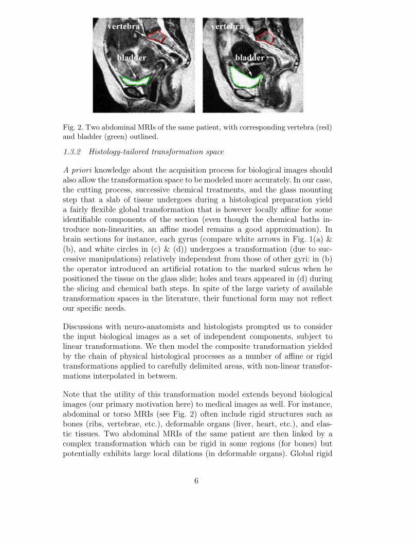
Fig. 2. Two abdominal MRIs of the same patient, with corresponding vertebra (red)and bladder (green) outlined.

1.3.2 Histology-tailored transformation space

A priori knowledge about the acquisition process for biological images shouldalso allow the transformation space to be modeled more accurately. In our case,the cutting process, successive chemical treatments, and the glass mountingstep that a slab of tissue undergoes during a histological preparation yielda fairly flexible global transformation that is however locally affine for someidentifiable components of the section (even though the chemical baths in-troduce non-linearities, an affine model remains a good approximation). Inbrain sections for instance, each gyrus (compare white arrows in Fig. 1(a) &(b), and white circles in (c) & (d)) undergoes a transformation (due to suc-cessive manipulations) relatively independent from those of other gyri: in (b)the operator introduced an artificial rotation to the marked sulcus when hepositioned the tissue on the glass slide; holes and tears appeared in (d) duringthe slicing and chemical bath steps. In spite of the large variety of availabletransformation spaces in the literature, their functional form may not reflectour specific needs.

Discussions with neuro-anatomists and histologists prompted us to considerthe input biological images as a set of independent components, subject tolinear transformations. We then model the composite transformation yieldedby the chain of physical histological processes as a number of affine or rigidtransformations applied to carefully delimited areas, with non-linear transfor-mations interpolated in between.

Note that the utility of this transformation model extends beyond biologicalimages (our primary motivation here) to medical images as well. For instance,abdominal or torso MRIs (see Fig. 2) often include rigid structures such asbones (ribs, vertebrae, etc.), deformable organs (liver, heart, etc.), and elas-tic tissues. Two abdominal MRIs of the same patient are then linked by acomplex transformation which can be rigid in some regions (for bones) butpotentially exhibits large local dilations (in deformable organs). Global rigid

6

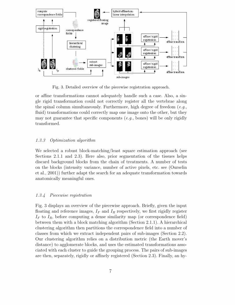
Fig. 3. Detailed overview of the piecewise registration approach.

or affine transformations cannot adequately handle such a case. Also, a sin-gle rigid transformation could not correctly register all the vertebrae alongthe spinal column simultaneously. Furthermore, high degree of freedom (e.g.,fluid) transformations could correctly map one image onto the other, but theymay not guarantee that specific components (e.g., bones) will be only rigidlytransformed.

1.3.3 Optimization algorithm

We selected a robust block-matching/least square estimation approach (seeSections 2.1.1 and 2.3). Here also, prior segmentation of the tissues helpsdiscard background blocks from the chain of treatments. A number of testson the blocks (intensity variance, number of active pixels, etc. see (Ourselinet al., 2001)) further adapt the search for an adequate transformation towardsanatomically meaningful ones.

1.3.4 Piecewise registration

Fig. 3 displays an overview of the piecewise approach. Briefly, given the inputfloating and reference images, IF and IR respectively, we first rigidly registerIF to IR, before computing a dense similarity map (or correspondence field)between them with a block matching algorithm (Section 2.1.1). A hierarchicalclustering algorithm then partitions the correspondence field into a number ofclasses from which we extract independent pairs of sub-images (Section 2.2).Our clustering algorithm relies on a distribution metric (the Earth mover’sdistance) to agglomerate blocks, and uses the estimated transformations asso-ciated with each cluster to guide the grouping process. The pairs of sub-imagesare then, separately, rigidly or affinely registered (Section 2.3). Finally, an hy-

7

brid affine/non-linear interpolation scheme is used to compose the registeredfloating image (Section 2.4).

Note that even though we specifically tailored the various modules of ourapproach to the problem at hand, namely the reconstruction of a 3-D histo-logical volume, most of them could be independently optimized or replaced ona need-for basis. For instance, the block-matching affine registration algorithmwe chose for the sub-images could be traded for another affine registration ap-proach from the literature. In that, the volume reconstruction system we pro-pose here can also be seen as a generic framework. However, care would haveto be taken not to compromise the overall homogeneity and robustness. Goodglobal robustness requires the selection or the development of robust modules.Homogeneity ensures that the best overall performances can be achieved fromindividual contributions.

We detail our method in Section 2 and discuss the reconstruction of two his-tological volumes in Section 3 along with the sensitivity of our algorithm tonoise conditions and parameters.

2 Method

The first step of our approach consists of automatically partitioning the inputfloating and reference images (IF and IR) into a number of pairs of correspond-ing sub-images, where each sub-image is associated with an independent (interms of transformation) image component.

We approach this segmentation issue as a process of partitioning a correspon-dence field computed from IF to IR. Our method is motivated by the followingobservation. When both images are composed of pairs of independent com-ponents, where each component is subject to some linear transformation, theassociated correspondence field should exhibit rather homogeneous character-istics within each component, and heterogeneous ones across them. Conse-quently, by clustering the fields with a criterion based on local characteristics,we hope to extract from them the desired independent components.

2.1 Computing the initial correspondence field

We use a block-matching algorithm (Jain, 1981) to compute the correspon-dence field. Block-matching was favored over classical non-linear registration

8

approaches as it offers better spatial independence between neighboring corre-spondences, as opposed to standard techniques whose regularization schemesinduce spatial correlations. Indeed, given the unpredictable nature of the in-put images (which may contain tears, holes, rotated sulci, etc.), we must allowfor independent variations of the correspondence field.

2.1.1 Block-matching algorithm

We associate with IF and IR two rectangular lattices LF = {(i, j) ∈ [1, . . . , wF ]×[1, . . . , hF ]} and LR = {(i′, j ′) ∈ [1, . . . , wR] × [1, . . . , hR]} respectively, whosesites correspond to pixels in the input images. We may choose to associate asite to each pixel of the input images, in which case wF , hF and wR, hR are thewidth and height of IF and IR, respectively. We could also consider a sparserregular or non-regular site distribution. In our case, we use sparse regular lat-tices and discard, for histological sections, sites which lie on the background. Aprior segmentation step is then required to identify these background blocks:depending on the modality and quality (in terms of signal to noise ratio, andcontrast) of the input images, we either use simple intensity thresholding (thecase for the myelin-stained human brain section of Fig. 1), or a more sophisti-cated segmentation algorithm (the neural classifier introduced in (Pitiot et al.,2002) for instance).

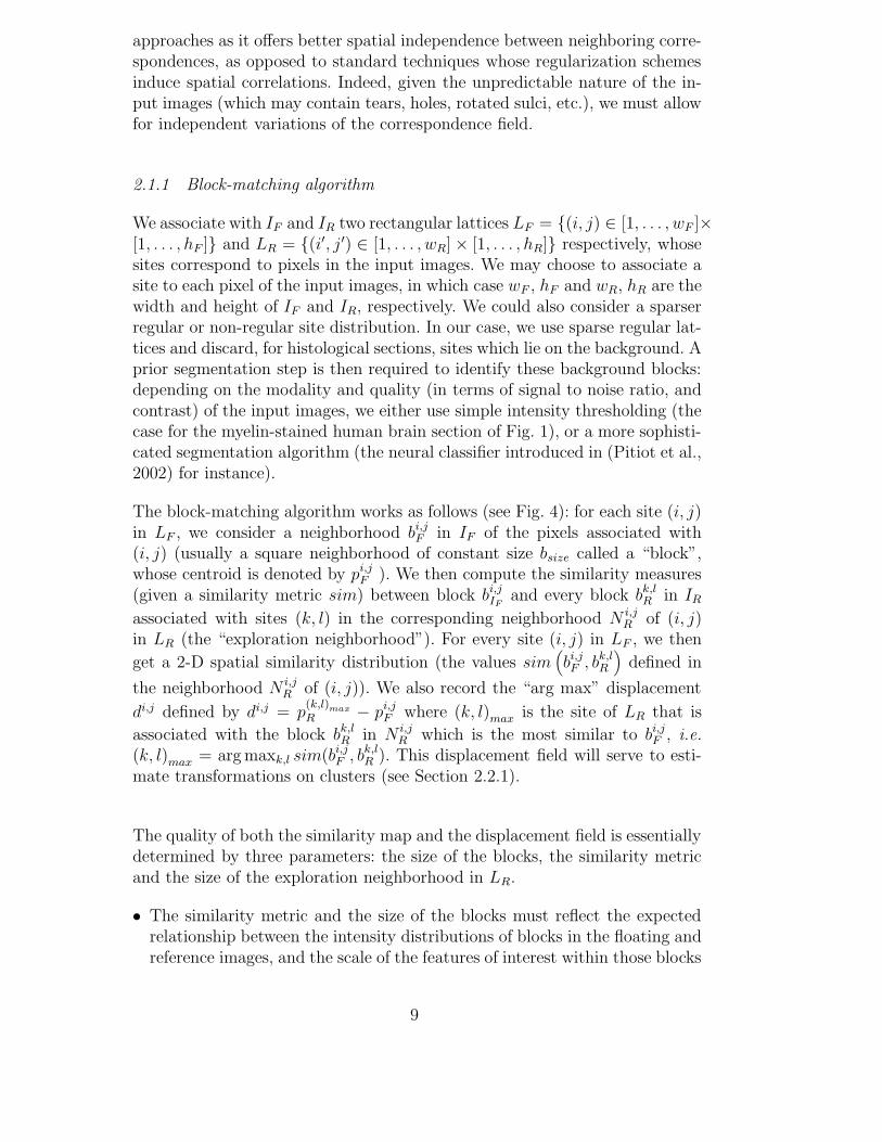
The block-matching algorithm works as follows (see Fig. 4): for each site (i, j)in LF , we consider a neighborhood bi,j

F in IF of the pixels associated with(i, j) (usually a square neighborhood of constant size bsize called a “block”,whose centroid is denoted by pi,j

F ). We then compute the similarity measures(given a similarity metric sim) between block bi,j

IFand every block bk,l

R in IR

associated with sites (k, l) in the corresponding neighborhood N i,jR of (i, j)

in LR (the “exploration neighborhood”). For every site (i, j) in LF , we then

get a 2-D spatial similarity distribution (the values sim(

bi,jF , bk,l

R

)

defined in

the neighborhood N i,jR of (i, j)). We also record the “arg max” displacement

di,j defined by di,j = p(k,l)max

R − pi,jF where (k, l)max is the site of LR that is

associated with the block bk,lR in N i,j

R which is the most similar to bi,jF , i.e.

(k, l)max = arg maxk,l sim(bi,jF , bk,l

R ). This displacement field will serve to esti-mate transformations on clusters (see Section 2.2.1).

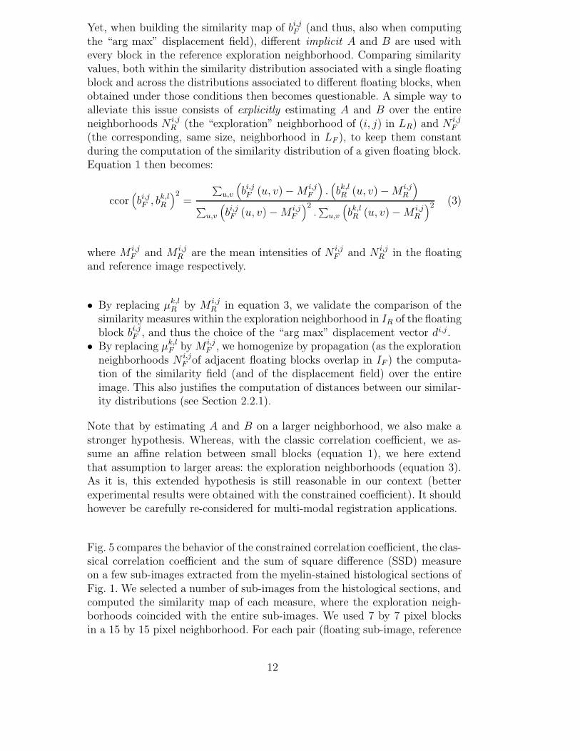
The quality of both the similarity map and the displacement field is essentiallydetermined by three parameters: the size of the blocks, the similarity metricand the size of the exploration neighborhood in LR.

• The similarity metric and the size of the blocks must reflect the expectedrelationship between the intensity distributions of blocks in the floating andreference images, and the scale of the features of interest within those blocks

9

Fig. 4. Block-matching algorithm

respectively (see (Collins et al., 2003) and (Dengler, 1991) for details).• The size of the exploration neighborhood is linked to the expected magni-

tude of the residual displacements after global alignment. It conditions theextent to which our registration algorithm can recover large deformations:the further apart corresponding components are, the larger the size of theneighborhood must be.

Section 3.2 comments on the impact of our algorithm’s parameters on theoverall registration quality. Please refer to Table 1 for some standard values.

As a pre-processing step, we first rigidly register IF to IR to remove fromthe subsequently computed correspondence fields the global rigid transformthat uniformly affects all components. We use the fully automated intensity-based registration algorithm presented in Ourselin et al. (2001), where a robust

multi-scale block-matching strategy was introduced. Not accounting for thiswould only degrade the quality of the field and affect the efficiency of theclustering.

2.1.2 Constrained correlation coefficient

A ubiquitous choice for image registration (Roche et al., 2000), the correlationcoefficient represents, in the context of block-matching, a measure of the affinedependency between the block of interest bi,j

F in the floating images and ev-ery block bk,l

R in the corresponding exploration neighborhood in the referenceimage. It is written:

cor(

bi,jF , bk,l

R

)2=

cov(

bi,jF , bk,l

R

)2

var(

bi,jF

)

.var(

bk,lR

) =

(

∑

u,v

(

bi,jF (u, v) − µi,j

F

)

.(

bk,lR (u, v) − µk,l

R

))2

∑

u,v

(

bi,jF (u, v) − µi,j

F

)2.∑

u,v

(

bk,lR (u, v) − µk,l

R

)2 (1)

where µi,jF and µk,l

R are the mean intensities of bi,jF and bk,l

R respectively. Tomake the affine dependency clearer, equation 1 can be rewritten (Roche et al.,

10

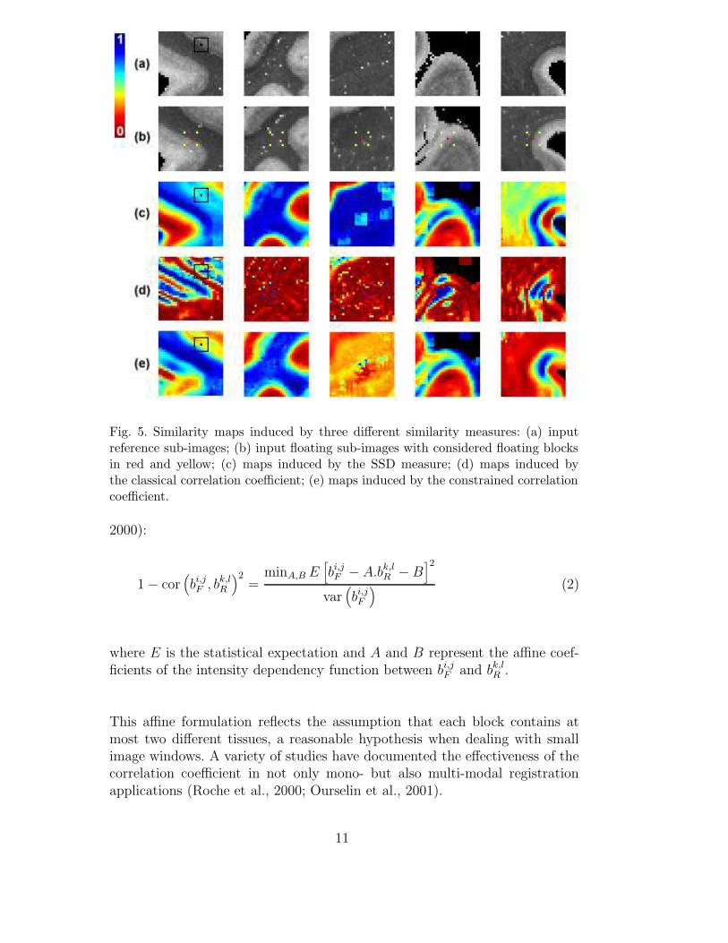
Fig. 5. Similarity maps induced by three different similarity measures: (a) inputreference sub-images; (b) input floating sub-images with considered floating blocksin red and yellow; (c) maps induced by the SSD measure; (d) maps induced bythe classical correlation coefficient; (e) maps induced by the constrained correlationcoefficient.

2000):

1 − cor(

bi,jF , bk,l

R

)2=

minA,B E[

bi,jF − A.bk,l

R − B]2

var(

bi,jF

) (2)

where E is the statistical expectation and A and B represent the affine coef-ficients of the intensity dependency function between bi,j

F and bk,lR .

This affine formulation reflects the assumption that each block contains atmost two different tissues, a reasonable hypothesis when dealing with smallimage windows. A variety of studies have documented the effectiveness of thecorrelation coefficient in not only mono- but also multi-modal registrationapplications (Roche et al., 2000; Ourselin et al., 2001).

11

Yet, when building the similarity map of bi,jF (and thus, also when computing

the “arg max” displacement field), different implicit A and B are used withevery block in the reference exploration neighborhood. Comparing similarityvalues, both within the similarity distribution associated with a single floatingblock and across the distributions associated to different floating blocks, whenobtained under those conditions then becomes questionable. A simple way toalleviate this issue consists of explicitly estimating A and B over the entireneighborhoods N i,j

R (the “exploration” neighborhood of (i, j) in LR) and N i,jF

(the corresponding, same size, neighborhood in LF ), to keep them constantduring the computation of the similarity distribution of a given floating block.Equation 1 then becomes:

ccor(

bi,jF , bk,l

R

)2=

∑

u,v

(

bi,jF (u, v) − M i,j

F

)

.(

bk,lR (u, v) − M i,j

R

)

∑

u,v

(

bi,jF (u, v) − M i,j

F

)2.∑

u,v

(

bk,lR (u, v) − M i,j

R

)2 (3)

where M i,jF and M i,j

R are the mean intensities of N i,jF and N i,j

R in the floatingand reference image respectively.

• By replacing µk,lR by M i,j

R in equation 3, we validate the comparison of thesimilarity measures within the exploration neighborhood in IR of the floatingblock bi,j

F , and thus the choice of the “arg max” displacement vector di,j.• By replacing µk,l

F by M i,jF , we homogenize by propagation (as the exploration

neighborhoods N i,jF of adjacent floating blocks overlap in IF ) the computa-

tion of the similarity field (and of the displacement field) over the entireimage. This also justifies the computation of distances between our similar-ity distributions (see Section 2.2.1).

Note that by estimating A and B on a larger neighborhood, we also make astronger hypothesis. Whereas, with the classic correlation coefficient, we as-sume an affine relation between small blocks (equation 1), we here extendthat assumption to larger areas: the exploration neighborhoods (equation 3).As it is, this extended hypothesis is still reasonable in our context (betterexperimental results were obtained with the constrained coefficient). It shouldhowever be carefully re-considered for multi-modal registration applications.

Fig. 5 compares the behavior of the constrained correlation coefficient, the clas-sical correlation coefficient and the sum of square difference (SSD) measureon a few sub-images extracted from the myelin-stained histological sections ofFig. 1. We selected a number of sub-images from the histological sections, andcomputed the similarity map of each measure, where the exploration neigh-borhoods coincided with the entire sub-images. We used 7 by 7 pixel blocksin a 15 by 15 pixel neighborhood. For each pair (floating sub-image, reference

12

sub-image), we show the associated similarity map in color. The comparisonof the three maps demonstrates the good compromise achieved by the con-strained coefficient between the regularity of the SSD and the good precisionof the classical correlation coefficient. The benefits of the constrained formu-lation over the classical one are particularly obvious in the third and fourthcolumn, where the correlation coefficient cannot manage a background com-posed of low variance blocks (high noise). Finally, comparison between maps(d) and (e) in the left-most column shows that while a high similarity value(dark blue) is obtained with the classical correlation coefficient for a pair ofblocks with inverted tissues (white matter in the bottom-left corner/ graymatter in the top-right corner of the floating block and the other way aroundfor the reference block, in black), a lower one (yellow) is obtained with theconstrained coefficient.

Fig. 6 displays the similarity distributions for both the constrained and theclassical correlation coefficient and the “arg max” displacement field (for theconstrained coefficient) for the two consecutive histological sections of thebrain of Fig. 1 (60 µm myelin stained coronal sections through the occipitalcortex). For every site of the floating lattice, a color square shows the similaritymeasures between the corresponding floating block and the reference blocks inits neighborhood (middle column). The optimal ”arg max” displacement fieldis rendered with arrows whose length and direction are those of the optimaldisplacement vector associated to the lattice site at which the arrow originates.For visualization purposes, only half of the “similarity squares” are renderedin the similarity maps. Obviously, the similarity squares associated to the con-strained coefficient present clear patterns (much clearer than those nonethelessexhibited by the classical coefficient), and, more importantly, conspicuous dif-ferences in patterns across the image, that will help the clustering algorithmsegment the input images. Additionally, the “arg max” displacement field, al-though globally rather chaotic, tends to present more homogeneous patternsat a local scale, from which transformations can be estimated in a robust fash-ion. This will help both cluster the input images and register the extractedsub-images.

2.2 Extracting the image components

A dense correspondence field has been computed as described in the previoussection. We further assume that the input floating image consists of com-ponents that share similar transformation characteristics. We describe herethe way the correspondence field is clustered, and how we extract sub-imagesfrom the clustered sites. Those sub-images will be later used to estimate localtransformations.

13

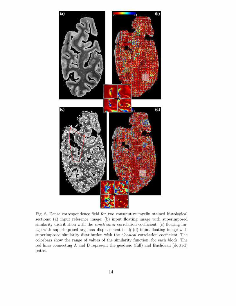
Fig. 6. Dense correspondence field for two consecutive myelin stained histologicalsections: (a) input reference image; (b) input floating image with superimposedsimilarity distribution with the constrained correlation coefficient; (c) floating im-age with superimposed arg max displacement field; (d) input floating image withsuperimposed similarity distribution with the classical correlation coefficient. Thecolorbars show the range of values of the similarity function, for each block. Thered lines connecting A and B represent the geodesic (full) and Euclidean (dotted)paths.

14

2.2.1 Clustering the correspondence field

We are looking for a hierarchical clustering of LF , that is, a sequence of parti-tions in which each partition is nested into the next partition in the sequence(Backer, 1995). Cluster analysis (unsupervised learning) essentially consists ofsorting a series of multi-dimensional points into a number of groups (clusters)so as to maximize the intra-cluster degree of association and minimize theinter-cluster one. It is particularly well suited here as it behaves adequatelyeven when very little is known about the category structure of the input setof points. That is, it does not require strong hypotheses to be formulatedbeforehand.

For simplicity’s sake, we rewrite LF as an ordered set of sites:

LF = {s suchthat ∃!(i, j) ∈ LF , s = (i, j)}wF .hF

t=1 .

Our clustering method is adapted from the standard agglomerative hierarchi-cal clustering algorithm described in (Johnson, 1967):

step 1: initialize a cluster list by placing each site of LF in an individual clus-ter, and let the distance between any two of those clusters be the distance(to be defined) between the sites they contain (the more similar the clusters,the smaller the distance).

step 2: find the closest pair of clusters, remove them from the cluster list,merge them into a new single cluster and add the new cluster to the clusterlist.

step 3: compute the distances between the newly formed cluster and theother ones in the cluster list.

step 4: repeat steps 2 and 3 until the desired number of clusters have beenreached.

In our case, the number of clusters is specified by the user. Pre-indicatorslike the Davies-Bouldin index (Davies and Bouldin, 1979) for instance, orthe cophenetic correlation coefficient (Backer, 1995) could possibly assist thischoice. Section 3.2 discusses the influence of this parameter over the registra-tion quality.

To store the distances between any two clusters in the cluster list at eachiteration, we maintain a variable-size distance matrix M which summarizestheir proximity (or similarity). At each iteration, M is therefore a squaresymmetric matrix whose size is the number of clusters in the cluster list atthat iteration. The computation of similarity matrix M is the pivotal elementof the clustering algorithm. The distance measure between clusters shouldbe consistent with both the model we chose for the input images and therelationships we expect between them.

15

To define a distance on clusters, we first need a distance on sites. This dis-tance is defined as a linear combination of two distances, a distance betweenthe centroids of the associated blocks and a distance between the associatedsimilarity distributions:

Dsite = α Dcentroid + (1 − α) Ddistribution (4)

Distance between the centroids. To satisfy the model constraint, we haveto ensure that close blocks are more likely to be clustered than blocks farapart. It appears that the Euclidean distance is not the most suitable here.Indeed, if the input images contain several pieces of tissues (e.g., in histologi-cal images, they can easily be identified by thresholding) that are potentiallynon convex, a geodesic distance within each piece will be more convenientto define the proximity of two points from an anatomical point of view.We recall that the geodesic distance between two points is the length ofthe shortest path that connects these points within a component that mustcontain them. By convention, when two sites cannot be connected (whenthey belong to disjoint components), we define the geodesic distance as theEuclidean distance between their associated centroids plus the radius of theinput image. Computation of the geodesic distances was done using a vari-ant of the circular propagation algorithm introduced in (Cuisenaire, 1999)which achieves a good trade-off of precision over speed.

Given two sites t and u, their centroid distance is written: Dcentroid (t, u) =Dgeodesic (pt

F , puF ).

Distance between similarity distributions. The high expressivity of thesimilarity distributions described above (Section 2.1), which summarize thesimilarity landscapes associated with the neighborhoods of the blocks ofinterest, makes them remarkably well suited to capture the actual differencesbetween those blocks, in spite of noise or decoys, and thus allows for abetter discrimination. We use a normalized version ρ of these distributionsto ensure that they all have the same overall unit mass (see (Singh andAllen, 1992) for a similar distributional approach in the context of image-flow computation).

Given a site t in LF , the associated 2-D normalized distribution ρt isdefined for sites u in the neighborhood Nt of t in LR by ρt (pu

R − ptF ) =

sim(btF

,buR)

∑

v ∈Ntsim(bt

F,bv

R). Such distributions are depicted in Fig. 6 (middle column).

As a distance between distributions, we chose the Earth mover’s distance(Rubner et al., 1998), a discrete solution to the discrete Monge-Kantorovichmass-transfer problem (Haker et al., 2003). Given the so-called “ground dis-tance” (the distance between elements of the distribution, the Euclideandistance in our case), the Earth mover’s distance (EMD) between two dis-tributions becomes the minimal total amount of work (= mass × distance)it takes to transform one distribution into the other. As argued by Rubneret al. (1998), this boils down to a bipartite network flow problem, which can

16

be modeled with linear programming and solved by a simplex algorithm.Among other advantages, the EMD is a true metric, is not impaired byquantization problems (as opposed to histogram-based approaches for in-stance) and can handle variable-size distributions (our case here). For sitest and u, we obtain: Ddistribution (t, u) = DEMD (ρt, ρu).

To summarize, given two sites t and u, their site distance is written:

Dsite (t, u) = α Dgeodesic

(

ptF , pu

F

)

+ (1 − α) DEMD

(

ρt, ρu)

(5)

where α is a real-valued positive weight (0 ≤ α ≤ 1).

Once we have a distance between sites, a cluster distance can be defined. Weadapted the standard complete link distance (Backer, 1995) to additionallytake into account the transformations that can be estimated on the alreadyformed clusters.

Namely, when the size of a cluster reaches a given threshold (we usually takeθcluster=20, even though experiments showed that the value of that thresholddoes not really impact the quality of the clustering), a rigid or affine trans-formation can be estimated, in a robust fashion, from the associated set of“arg max” displacement vectors (via a least-square regression combined withan LTS (Least Trimmed Squares) estimator, see Section 2.4). The decision tomerge two clusters can then be biased by the agreements between their associ-ated estimated transformations, again as this might indicate that they belongto the same component. Incidentally, when the distance between a cluster withan associated transformation and another one without enough sites to haveallowed an estimation must be computed, we choose to return 0. Althoughtheoretically possible, such a case almost never occurs in practice as a hierar-chical clustering algorithm tends to aggregate sites in small clusters at earlystages before merging them into large ones in subsequent iterations, not leav-ing single sites un-aggregated very long (see (Backer, 1995) for details). Thisso-called “chaining effect” also motivates the use of transformation distances.

Given two transformations T a and T b, we use a standard symmetric distance:

Dtrsf

(

T a, T b)

=

∑

i,j

[

T aT b−1− Id

]2

i,j+

∑

i,j

[

T a−1T b − Id]2

i,jif both T a and T b are defined

0 otherwise(6)

(where i, j are matrix indices).

Finally, given two clusters of sites Ca = {a1, . . . , ana} and Cb = {b1, . . . , bnb

},

17

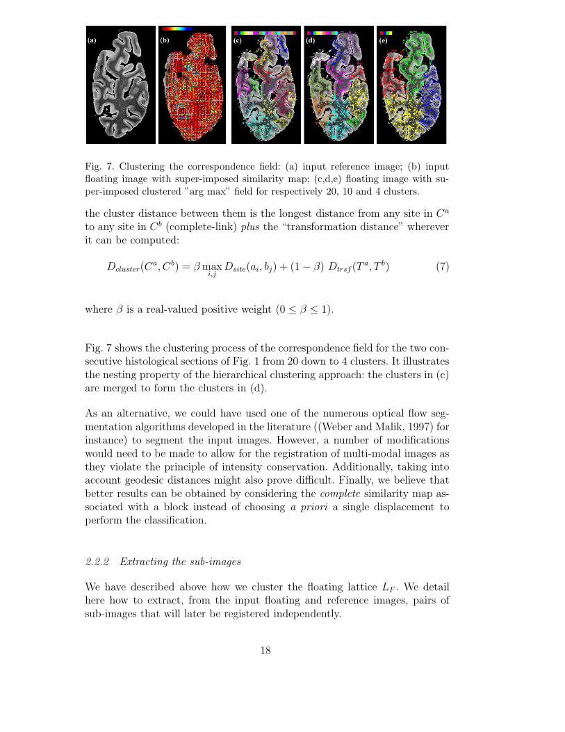
Fig. 7. Clustering the correspondence field: (a) input reference image; (b) inputfloating image with super-imposed similarity map; (c,d,e) floating image with su-per-imposed clustered ”arg max” field for respectively 20, 10 and 4 clusters.

the cluster distance between them is the longest distance from any site in Ca

to any site in Cb (complete-link) plus the “transformation distance” whereverit can be computed:

Dcluster(Ca, Cb) = β max

i,jDsite(ai, bj) + (1 − β) Dtrsf(T

a, T b) (7)

where β is a real-valued positive weight (0 ≤ β ≤ 1).

Fig. 7 shows the clustering process of the correspondence field for the two con-secutive histological sections of Fig. 1 from 20 down to 4 clusters. It illustratesthe nesting property of the hierarchical clustering approach: the clusters in (c)are merged to form the clusters in (d).

As an alternative, we could have used one of the numerous optical flow seg-mentation algorithms developed in the literature ((Weber and Malik, 1997) forinstance) to segment the input images. However, a number of modificationswould need to be made to allow for the registration of multi-modal images asthey violate the principle of intensity conservation. Additionally, taking intoaccount geodesic distances might also prove difficult. Finally, we believe thatbetter results can be obtained by considering the complete similarity map as-sociated with a block instead of choosing a priori a single displacement toperform the classification.

2.2.2 Extracting the sub-images

We have described above how we cluster the floating lattice LF . We detailhere how to extract, from the input floating and reference images, pairs ofsub-images that will later be registered independently.

18

Let NC be the final number of clusters, C ={

C1, . . . , CNC

}

the cluster parti-

tion of LF , and{

ci1, . . . , c

ini

}

the ni sites of the ith cluster C i. We want to build

a set of NC sub-images {I iF}

NC

i=1, each of them associated with a single cluster.Given the partition of LF , a partition of IF can be built in many ways. Forinstance, one could compute a Voronoı diagram of the sites cj

i (or equivalentlyof their centroids) and draw a partition of the pixels (x, y) of IF from it. How-ever, our clustering method does not ensure that the borders between clustersare sufficiently precise to adequately represent the sub-images’ borders. More-over, as we are going to use these sub-images to find local transformations, itis often better to choose larger supports to avoid boundary effects.

Consequently, rather than build a partition of IF from the partition of LF , webuild a covering of IF , i.e., a set of sub-images that could overlap. To do so,we aggregate in I i

F the pixels of IF in the vicinity of the sites of the clusterCi. We get:

I iF = {(x, y) ∈ IF such that D((x, y), ci

j) ≤ coverradius for some cij ∈ Ci}(8)

In practice we use the L∞ distance. Then, with blocks of size bsize associated to

the sites, taking coverradius = bsize/2 we get I iF =

⋃

j bcij

IF. In our experiments,

to ensure a large support, we chose coverradius = 3/4 bsize.

The corresponding reference sub-images I iR are built identically, but with the

centroids p(k,l)max

R of the most similar blocks (see Section 2.1):

I iR = {(x, y) ∈ IR such that D((x, y), ci

j + dcij) ≤ coverradius, for some ci

j ∈ Ci}(9)

Again, we use the L∞ distance here, with coverradius = bsize (a larger ex-tent than that of the floating sub-image) to ensure that I i

F can be effectivelyregistered against I i

R.

2.3 Registering the sub-images

Once we have extracted the reference and floating sub-images, we use therobust affine block-matching algorithm described in (Ourselin et al., 2001)to register them, independently, pair by pair. Briefly, this algorithm first esti-mates a sparse “arg max” displacement field, using a block matching approach(our block-matching algorithm is closely derived from this approach, and wefeed both of them the same parameters and similarity measure). From thisfield, a least square regression extracts a rigid or an affine transformation. As

19

an illustration, in the rigid case we are looking for R∗ and t∗ such that:

(R∗, t∗) = arg minR,t

∑

i,j

∥

∥

∥

(

pi,jF + di,j

)

− R.pi,jF − t

∥

∥

∥

2(10)

where(

pi,jF + di,j

)

− Rpi,jF − t is the residual error and ‖.‖ the L2 Euclidean

norm.

However, given the rather noisy appearance of the displacement field, an LTSestimator (Least Trimmed Squares, see (Rousseeuw, 1984) for details) is usedin place of the least square one to ensure a robust estimation of the trans-formation. At a glance, instead of minimizing the total sum of the squaredresiduals (equation 10), a LTS estimator will iteratively minimize the sum ofthe h smallest squared residuals (we take h at 50% of the number of residuals),to reduce the influence of outliers.

Finally, a better trade-off between robustness and registration precision isachieved via a multi-scale implementation. Note that even though this block-matching algorithm computes displacements (actually, translations) only lo-

cally, it is able to recover global rotations and translations, thanks to its itera-tive nature. For instance, a robustness study on rat brains sections presentedin (Ourselin et al., 2001) demonstrated its ability to recover rotations up to28 degrees.

Then, for each pair of sub-images{

I lR, I l

F

}

, l ∈ 1 . . . NC , we obtain a rigid

or an affine transform T l. Note that since these registrations are robust, thesub-images do not need to perfectly correspond to the anatomically separatecomponents.

2.4 Composing the final images

We selected the method of Little et al. (1997) to compose the final regis-tered floating image. In their approach, a user selects a number of pairs ofcorresponding rigid structures in the input images along with associated lin-ear transformations (also given by the user). A number of pairs of landmarksfurther constrain a hybrid affine/non-linear interpolation scheme that acts asa local registration algorithm. This technique then essentially applies user-provided affine transforms to user-defined structures and ensures a smoothinterpolation in between them.

20

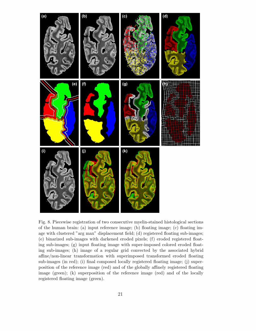
Fig. 8. Piecewise registration of two consecutive myelin-stained histological sectionsof the human brain: (a) input reference image; (b) floating image; (c) floating im-age with clustered ”arg max” displacement field; (d) registered floating sub-images;(e) binarized sub-images with darkened eroded pixels; (f) eroded registered float-ing sub-images; (g) input floating image with super-imposed colored eroded float-ing sub-images; (h) image of a regular grid convected by the associated hybridaffine/non-linear transformation with superimposed transformed eroded floatingsub-images (in red); (i) final composed locally registered floating image; (j) super-position of the reference image (red) and of the globally affinely registered floatingimage (green); (k) superposition of the reference image (red) and of the locallyregistered floating image (green).

21

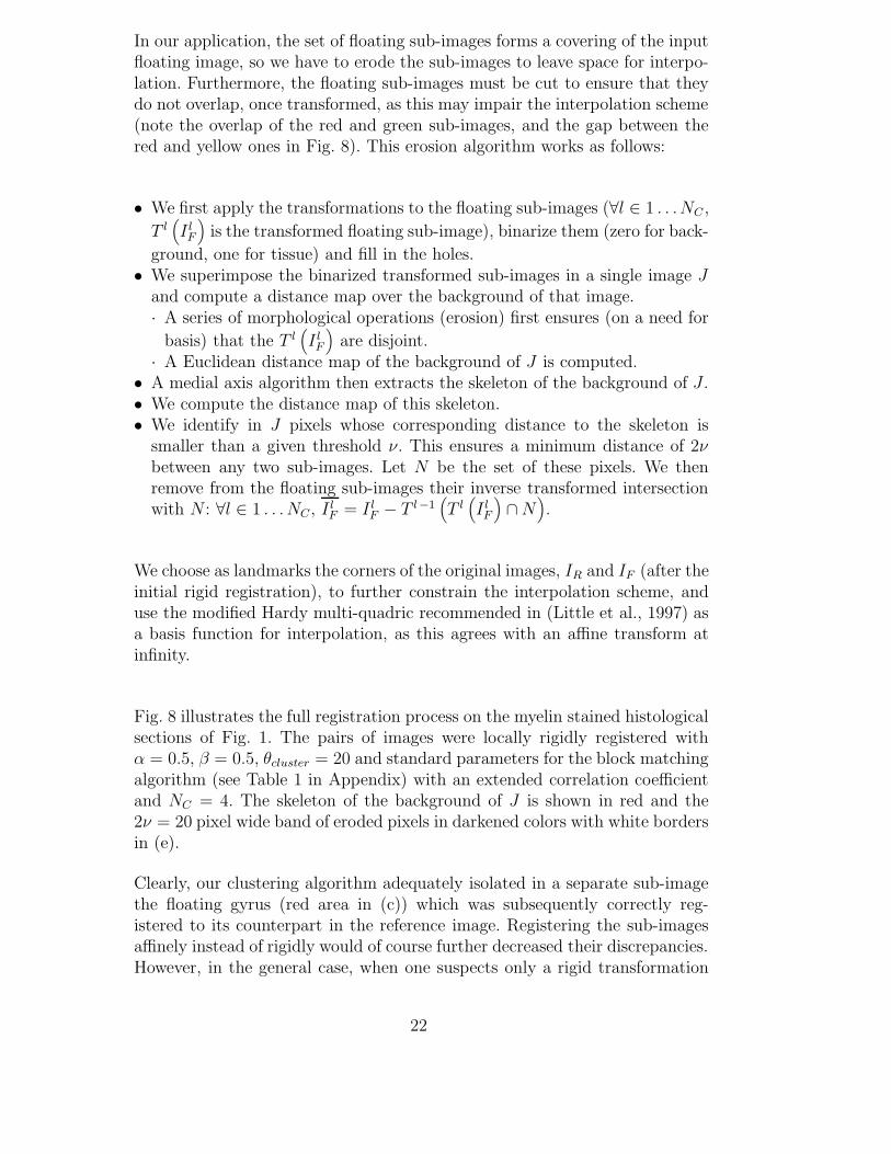
In our application, the set of floating sub-images forms a covering of the inputfloating image, so we have to erode the sub-images to leave space for interpo-lation. Furthermore, the floating sub-images must be cut to ensure that theydo not overlap, once transformed, as this may impair the interpolation scheme(note the overlap of the red and green sub-images, and the gap between thered and yellow ones in Fig. 8). This erosion algorithm works as follows:

• We first apply the transformations to the floating sub-images (∀l ∈ 1 . . .NC ,

T l(

I lF

)

is the transformed floating sub-image), binarize them (zero for back-

ground, one for tissue) and fill in the holes.• We superimpose the binarized transformed sub-images in a single image J

and compute a distance map over the background of that image.· A series of morphological operations (erosion) first ensures (on a need for

basis) that the T l(

I lF

)

are disjoint.· A Euclidean distance map of the background of J is computed.

• A medial axis algorithm then extracts the skeleton of the background of J .• We compute the distance map of this skeleton.• We identify in J pixels whose corresponding distance to the skeleton is

smaller than a given threshold ν. This ensures a minimum distance of 2νbetween any two sub-images. Let N be the set of these pixels. We thenremove from the floating sub-images their inverse transformed intersectionwith N : ∀l ∈ 1 . . . NC , I l

F = I lF − T l−1

(

T l(

I lF

)

∩ N)

.

We choose as landmarks the corners of the original images, IR and IF (after theinitial rigid registration), to further constrain the interpolation scheme, anduse the modified Hardy multi-quadric recommended in (Little et al., 1997) asa basis function for interpolation, as this agrees with an affine transform atinfinity.

Fig. 8 illustrates the full registration process on the myelin stained histologicalsections of Fig. 1. The pairs of images were locally rigidly registered withα = 0.5, β = 0.5, θcluster = 20 and standard parameters for the block matchingalgorithm (see Table 1 in Appendix) with an extended correlation coefficientand NC = 4. The skeleton of the background of J is shown in red and the2ν = 20 pixel wide band of eroded pixels in darkened colors with white bordersin (e).

Clearly, our clustering algorithm adequately isolated in a separate sub-imagethe floating gyrus (red area in (c)) which was subsequently correctly reg-istered to its counterpart in the reference image. Registering the sub-imagesaffinely instead of rigidly would of course further decreased their discrepancies.However, in the general case, when one suspects only a rigid transformation

22

between sub-images, opting for an affine registration would only introduceunnecessary over-parameterization which, among other disadvantages, couldsubstantially alter textures.

Note that the entire registration process could easily be included within aniterative multi-scale framework to achieve a better trade-off between accuracyand complexity. Such a framework could also be useful for handling bothlarge-scale and small-scale components.

3 Results

We present here the various experiments we have conducted to assess theperformances of our local registration approach. We detail two histologicalreconstructions (Section 3.1) before discussing in Section 3.2 the influenceof the various components and parameters of our registration system on thequality of the registration.

3.1 Reconstruction of a 3-D histological volume

Even though the deformations recovered by our registration method maysometimes be rather subtle, as exemplified by the registration of the pairof myelin-stained sections (Fig. 8), they become a clear nuisance when entirestacks of sections must be aligned.

We aim here to reconstruct a 3-D volume from a series of histological images.Previous work (Ourselin et al., 2001; Malandain et al., 2004) showed that byregistering (affinely or rigidly) each pair of consecutive slices in the stack wecan recover a geometrically coherent 3-D alignment of the 2-D images andprovide a satisfying 3-D reconstruction. However, local rigid/affine piece-wisetransformations, as described in the Introduction Section, still impair this reg-istration process and must be accounted for.

As an illustration of the benefits of our piece-wise approach, we first describethe reconstruction of a 3-D histological volume from a series of 70 images.These were 50µm thick myelin-stained histological sections of the human braincut in the V1 area. Reconstruction was performed using the classic pair-wiseapproach described above. This process requires the choice of a reference sec-tion: if we let Img(ref) be this reference section, with 1 < ref < 70, thereconstruction algorithm is then as follows:

23

for i from ref+1 upto 70

rigid piece-wise register Img(i) to Img(i-1)

for i from ref-1 downto 1

rigid piece-wise register Img(i) to Img(i+1)

Consequently, the quality of the overall reconstruction depends on the charac-teristics of the reference section, which should therefore be selected with greatcare. Indeed, any hole, tear or arbitrary distortion in the reference image isbound to affect the reconstructed 3-D volume. However, in the absence of anexternal anatomical reference, such a 3-D volume can only be reconstructedupto the transformation associated with the reference image. When an exter-nal reference is available, anatomical information can be exploited to guidethe registration process (Malandain et al., 2004).

We used here the same parameters as for the registration of the myelin-stainedsections of Fig. 8: α = 0.5, β = 0.5, θcluster = 20 and standard parameters forthe block matching algorithm with the constrained correlation coefficient andNC = 6.

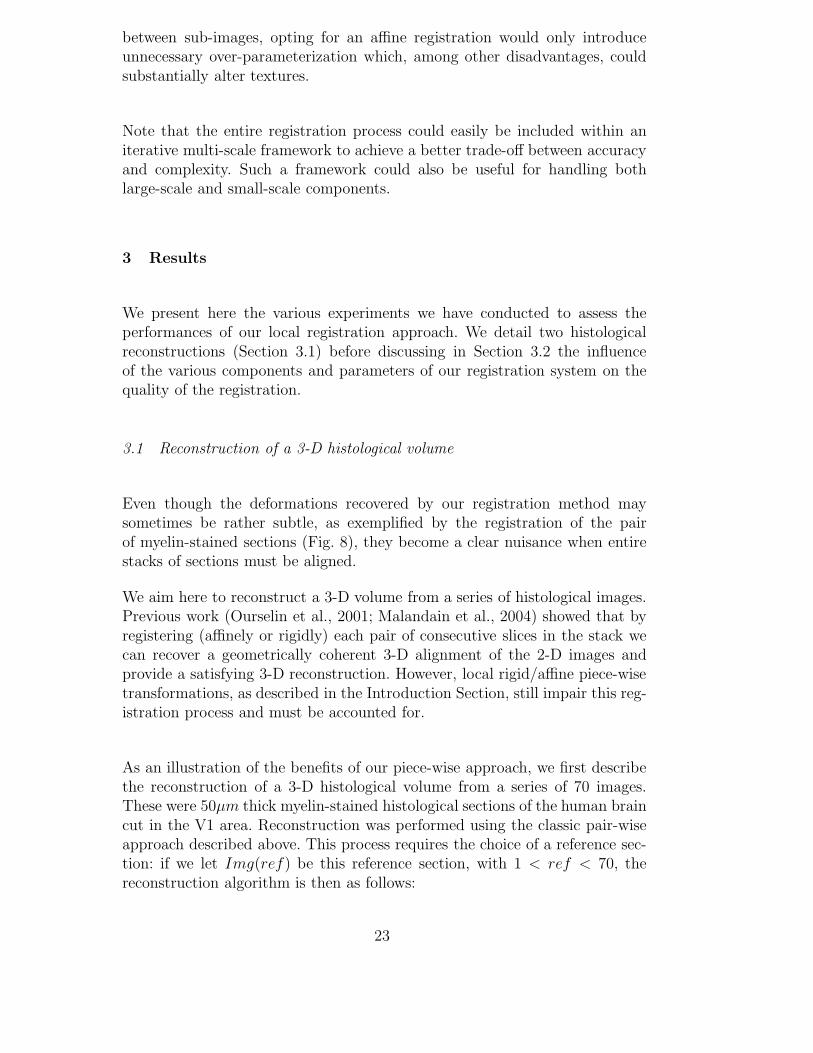
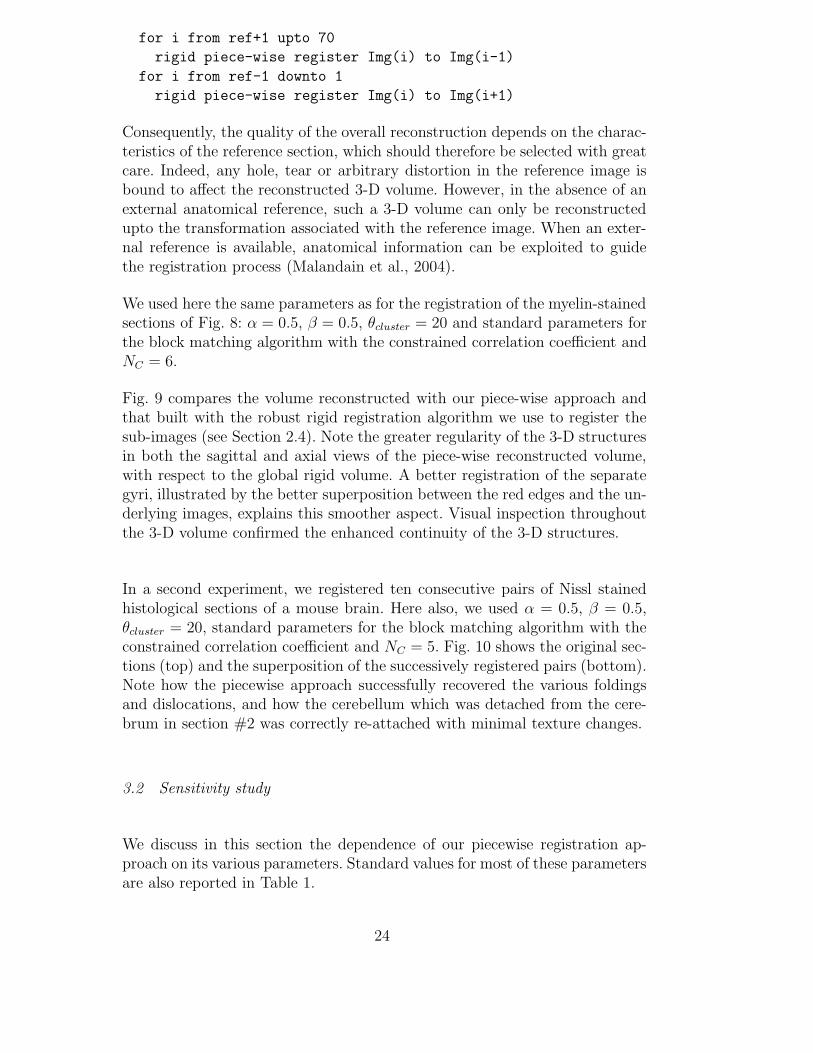
Fig. 9 compares the volume reconstructed with our piece-wise approach andthat built with the robust rigid registration algorithm we use to register thesub-images (see Section 2.4). Note the greater regularity of the 3-D structuresin both the sagittal and axial views of the piece-wise reconstructed volume,with respect to the global rigid volume. A better registration of the separategyri, illustrated by the better superposition between the red edges and the un-derlying images, explains this smoother aspect. Visual inspection throughoutthe 3-D volume confirmed the enhanced continuity of the 3-D structures.

In a second experiment, we registered ten consecutive pairs of Nissl stainedhistological sections of a mouse brain. Here also, we used α = 0.5, β = 0.5,θcluster = 20, standard parameters for the block matching algorithm with theconstrained correlation coefficient and NC = 5. Fig. 10 shows the original sec-tions (top) and the superposition of the successively registered pairs (bottom).Note how the piecewise approach successfully recovered the various foldingsand dislocations, and how the cerebellum which was detached from the cere-brum in section #2 was correctly re-attached with minimal texture changes.

3.2 Sensitivity study

We discuss in this section the dependence of our piecewise registration ap-proach on its various parameters. Standard values for most of these parametersare also reported in Table 1.

24

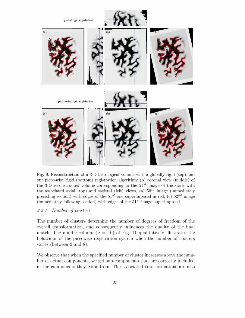
Fig. 9. Reconstruction of a 3-D histological volume with a globally rigid (top) andour piece-wise rigid (bottom) registration algorithm: (b) coronal view (middle) ofthe 3-D reconstructed volume corresponding to the 51st image of the stack withthe associated axial (top) and sagittal (left) views, (a) 50th image (immediatelypreceding section) with edges of the 51st one superimposed in red, (c) 52nd image(immediately following section) with edges of the 51st image superimposed

3.2.1 Number of clusters

The number of clusters determine the number of degrees of freedom of theoverall transformation, and consequently influences the quality of the finalmatch. The middle column (ν = 10) of Fig. 11 qualitatively illustrates thebehaviour of the piecewise registration system when the number of clustersvaries (between 2 and 8).

We observe that when the specified number of cluster increases above the num-ber of actual components, we get sub-components that are correctly includedin the components they come from. The associated transformations are also

25

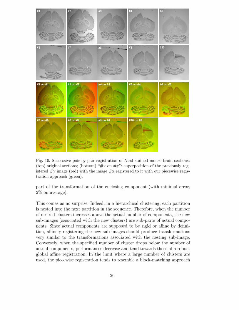
Fig. 10. Successive pair-by-pair registration of Nissl stained mouse brain sections:(top) original sections; (bottom) “#x on #y”: superposition of the previously reg-istered #y image (red) with the image #x registered to it with our piecewise regis-tration approach (green).

part of the transformation of the enclosing component (with minimal error,2% on average).

This comes as no surprise. Indeed, in a hierarchical clustering, each partitionis nested into the next partition in the sequence. Therefore, when the numberof desired clusters increases above the actual number of components, the newsub-images (associated with the new clusters) are sub-parts of actual compo-nents. Since actual components are supposed to be rigid or affine by defini-tion, affinely registering the new sub-images should produce transformationsvery similar to the transformations associated with the nesting sub-image.Conversely, when the specified number of cluster drops below the number ofactual components, performances decrease and tend towards those of a robustglobal affine registration. In the limit where a large number of clusters areused, the piecewise registration tends to resemble a block-matching approach

26

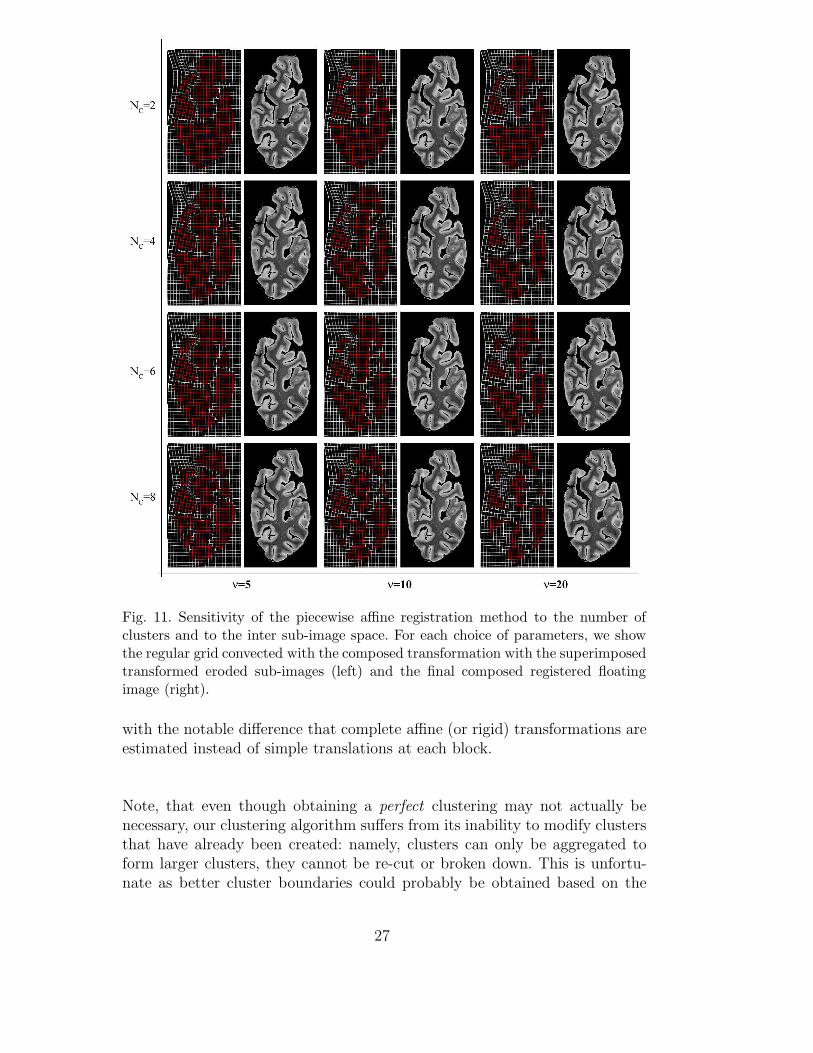
Fig. 11. Sensitivity of the piecewise affine registration method to the number ofclusters and to the inter sub-image space. For each choice of parameters, we showthe regular grid convected with the composed transformation with the superimposedtransformed eroded sub-images (left) and the final composed registered floatingimage (right).

with the notable difference that complete affine (or rigid) transformations areestimated instead of simple translations at each block.

Note, that even though obtaining a perfect clustering may not actually benecessary, our clustering algorithm suffers from its inability to modify clustersthat have already been created: namely, clusters can only be aggregated toform larger clusters, they cannot be re-cut or broken down. This is unfortu-nate as better cluster boundaries could probably be obtained based on the

27

associated cluster transformations, which are computed only after the clus-ters have reached a sufficient size to ensure a correct estimation. The useof stochastic clustering approaches or the introduction of uncertainty in theclustering process may alleviate this issue.

3.2.2 Block-matching parameters

As argued above, the quality of the similarity map computed between thefloating and the reference image depends on the block matching parameters:similarity measure, size of the exploration neighborhood, step in that neigh-borhood, size of blocks, etc. We already studied in Section 2.1.2 how the use ofa constrained correlation coefficient helped increase both the homogeneity andthe precision of the similarity map. Our block-matching algorithm is similar tothat detailed in (Ourselin et al., 2001), (Ourselin, 2002) and (Malandain et al.,2004) to which we report the reader for a detailed sensitivity investigation ofthe other parameters.

Note that the selection of the “arg max” displacement vector is clearly sub-optimal and somewhat arbitrary when many blocks in the reference explo-ration neighborhood have close associated similarity measures. Better esti-mation of the sub-image transformations might be obtained by taking intoaccount the full spectrum of displacement vectors, together with their simi-larity measures.

3.2.3 Parameters of the registration algorithm for the sub-images

The robust affine block-matching algorithm used in Section 2.3 to register thesub-images too requires that a number of parameters be set. In addition toblock matching parameters similar to ours, the cut-off of the robust estimator,the parameters controlling the multi-scale system within which it works, orthe parameters of the various variance and intensity tests performed on theblock to discard them from the robust estimation must be managed. Again,we report the reader to (Ourselin, 2002) for details about their influence onthe registration performances.

3.2.4 Composition parameters

The choice of the amount of space to leave in between structures (2ν pixels)depends on the input images and should be set accordingly. However, thereis no general prescription for selecting a good value for ν which would workwell for all images and, within a single image, for all sub-images. Clearly, asthe amount of space decreases, the band in between sub-images becomes morestretched (which might induce substantial textural changes).

28

Fig. 11 illustrates the relationships between the selected number of clustersand the space to leave between sub-images. As a rule of thumb, the greater thenumber of clusters is, the smaller ν should be, as the size of the componentstend to decrease. Note that even though we restricted ourselves to a constantvalue for ν across the image in this study, a variable ν should increase the over-all registration performances. Namely, for each pair of sub-images, ν shoulddepend on the differences between the transformations associated to the sub-images. If the difference is large, then a large ν is to be used to prevent largedistortions of the textures of the underlying tissues. Conversely, when the twosub-images share very similar transformations (even though these transforma-tion might be large with respect to the identity), ν can be much smaller (forinstance, for components A and B in Fig. 11).

The choice of ν could also depends on the nature of the underlying material:large deformations will not impair the quality of the registration if they occurover the black background. Use of tissue/background segmentation maps couldthen also help choose locally an optimal value for ν.

3.3 Specificity versus genericity

As argued in Section 1.2, the ill-posed nature of the medical image registra-tion problem makes it difficult to evaluate a posteriori the performance ofany given registration algorithm. This difficulty is essentially due to that ofcharacterizing an appropriate measure of performance. We submit that sincewe cannot trust the registration result, we must at least have confidence in theregistration method. A safe approach then consists of devising a registrationmodel which mimics, at the desired scale, the actual transformation under-gone by the imaged tissues. Prior medical knowledge is then pivotal in helpingdesign such a specific registration method. This concept of trust becomes es-pecially relevant in the context of high throughput registration (our case heresince reconstructing a volume requires registering a large number of images)where the quality of each registration results affects that of the subsequentones.

For histological reconstruction, our piecewise model adequately recovers thearbitrarily large transformations introduced during the glass mounting step,while allowing flexible deformations at the interface between anatomical re-gions. As mentioned before, a number of fluid or elastic approaches could beapplied to the same histological reconstruction problem with most certainlyvery similar visual results once their parameters have been tuned. However,given their inherently generic nature, only somewhat indirect control could beexerted over the registration process. It is thus difficult to weight the contri-butions of the various parts of the image in the process and how they interact

29

with the registration algorithm. In particular, the resulting transformationmay exhibit local deformations in unexpected locations. For instance, onemight wonder if and how the background was discarded, or whether particu-larly bright lesions or tumors did not heavily biased the joint histogram fromwhich mutual information or correlation ratio were computed, etc.

Incidentally, our piecewise approach is also more economical in terms of de-grees of freedom than a typical fluid one.

4 Conclusion

We have presented an automated 3D volume reconstruction methodologybased on the pair-by-pair registration of consecutive 2D images. Our methodrelies on the modeling of the actual transformation undergone by the imagedtissues in each section. In view of the ill-posed nature of image registration,we believe that specific registration techniques, which closely model the ac-tual physical transformations, are more suitable than generic all-purpose al-gorithms for reconstruction.

In the case of histological sections, our system builds complex spatial trans-formations by elastically interpolating between rigid or affine transforms thatare locally defined on pairs of sub-images. These sub-images represent geomet-rically, and often anatomically, coherent components. They are automaticallyextracted from an initial displacement field computed between the images tobe registered (by contrast with other approaches (Little et al., 1997)).

The use of a hierarchical clustering approach and a similarity distributiondistance proved very promising: while the distribution distance can effectivelydeal with noise and textural issues to discriminate between image blocks, ourclustering algorithm manages to extract the expected sub-images.

Finally, preliminary experiments have also shown that the developed approachworked well on multi-modal registration cases (Pitiot et al., 2003b,a).

Acknowledgement

This work was partially funded by European project MAPAWAMO (ref. QLG3-CT-2000-30161). Grant support for AP and PT was provided by a P41 Re-source Grant from the National Center for Research Resources (RR13642), theNational Library of Medicine (LM05639), the National Institute for Biomed-ical Imaging and Bioengineering (EB001561) and by a Human Brain Project

30

grant to the International Consortium for Brain Mapping, funded jointly byNIMH and NIDA (MH52176). AP was also supported by the INRIA associatedteam grant.

The authors would like to thank J. Annese from the LONI laboratory for pro-viding the human brain sections, and Y.Z. Wadghiri, J. Blind and D. Turnbullfrom the Skirball Institute at NYU for the mouse brain images.

Appendix

Standard values

Table 1 reports standard values for the various parameters of the algorithmswe use in our approach.

References

Arsigny, V., Pennec, X., Ayache, N., 2003. Polyrigid and Polyaffine Transfor-mations: A New Class of Diffeomorphisms for Locally Rigid or Affine Reg-istration. In: Proc. of Medical Image Computing and Computer-AssistedIntervention (MICCAI’03). pp. 829–837.

Ashburner, J., Friston, K. J., 1999. Nonlinear Spatial Normalization UsingBasis Functions. Human Brain Mapping 7 (4), 254–266.

Backer, E., 1995. Computer-Assisted Reasoning in Cluster Analysis. PrenticeHall.

Cachier, P., 2002. Recalage Non Rigide d’Images Mdicales Volumiques - Con-tribution aux Approches Iconiques et Gomtriques. Ph.D. thesis, Ecole Cen-trale des Arts et Manufactures.

Christensen, G. E., 1999. Consistent Linear-Elastic Transformations for Im-age Matching. In: Proc. of Information Processing in Medical Imaging(IPMI’99). pp. 224–237.

Cohen, F., Yang, Z., Huang, Z., Nissanov, J., 1998. Automatic Matching ofHomologous Histological Sections. IEEE Transaction on Biomedical Engi-neering 45 (5), 642–649.

Collignon, A., Maes, F., Delaere, D., Vandermeulen, D., Suetens, P., Marchal,G., 1995. Automated multimodality image registration using informationtheory. In: Proc. of Information Processing in Medical Imaging (IPMI’95).pp. 263–274.

Collins, D. L., Evans, A. C., Holmes, C., Peters, T. M., 1995. Automatic3D Segmentation of Neuro-anatomical Structures from MRI. In: Proc. ofInformation Processing in Medical Imaging (IPMI’95). pp. 139–152.

31

Collins, D. L., Zijdenbos, A. P., Paus, T., Evans, A. C., 2003. Use of Regis-tration for Cohort Studies. In: Medical Image Registration.

Cuisenaire, O., 1999. Distance Transformations: Fast Algorithms and Appli-cations to Medical Image Processing. Ph.d. thesis.

Davatzikos, C., 1997. Spatial Transformation and Registration of Brain Imagesusing Elastically Deformable Models. Computer Vision and Image Under-standing 66 (2), 207–222.

Davies, D. L., Bouldin, D. W., 1979. A Cluster Separation Measure. IEEETransactions on Pattern Analysis and Machine Intelligence 1, 224–227.

Dengler, J., 1991. Estimation of Discontinuous Displacement Vector Fieldswith the Minimum Description Length Criterion. In: IEEE Conference onComputer Vision and Pattern Recognition (CVPR’91). pp. 276–282.

Deverell, M., Salisbury, J., Cookson, M., Holman, J., Dykes, E., Whimster,F., 1993. Three-Dimensional Reconstruction: Methods of Improving ImageRegistration and Interpretation. Analytical Cellular Pathology 5 (5), 253–263.

Feldmar, J., Ayache, N., 1996. Rigid, Affine and Locally Affine Registration ofFree-Form Surfaces. The International Journal of Computer Vision 18 (2).

Ford-Holevinski, T., Castle, M., Herman, J., Watson, S., 1991. Microcomputer-based three-dimensional reconstruction of in situ hybridization autoradio-graphs. Journal of Chemical Neuroanatomy 4 (5), 373–385.

Gee, J. C., Reivich, M., Bajcsy, R., 1993. Elastically Deforming 3D Atlas toMatch Anatomical Brain Images. Journal of Computer Assisted Tomogra-phy 17 (2), 225–236.

Goldszal, A., Tretiak, O., Hand, P., Bhasin, S., McEachron, D., 1995. Three-Dimensional Reconstruction of Activated Columns from 2-[14C]deoxy-D-glucose Data. Neuroimage 2 (1), 9–20.

Goldszal, A., Tretiak, O., Liu, D., Hand, P., 1996. Multimodality Multidi-mensional Image Analysis of Cortical and Subcortical Plasticity in the RatBrain. Annal of Biomedical Engineering 24 (3), 430–439.

Haker, S., Angenent, S., Tannenbaum, A., 2003. Minimizing Flows for theMonge-Kantorovich Problem. SIAM Journal of Mathematical Analysis35 (1), 61–97.

Haney, S., Thompson, P., Cloughesy, T., Alger, J., Toga, A., 2001. TrackingTumor Growth Rates in Patients with Malignant Gliomas: A Test of TwoAlgorithms. American Journal of Neuroradiology 22 (1), 73–82.

Hibbard, L., Hawkins, R., 1988. Objective Image Alignment for Three-Dimensional Reconstruction of Digital Autoradiograms. Journal of Neuro-science Methods 26 (1), 55–74.

Humm, J., Macklis, R., Lu, X., Yang, Y., Bump, K., Beresford, B., Chin,L., 1995. The Spatial Accuracy of Cellular Dose Estimates Obtained from3D Reconstructed Serial Tissue Autoradiographs. Physics in Medicine andBiology 40 (1), 163–180.

Jain, A. K., 1981. Image Data Compression: A Review. Proceedings of theIEEE 69 (3), 349–389.

32

Johnson, S. C., 1967. Hierarchical Clustering Schemes. Psychometrika 32, 241–254.

Jolesz, F. A., Nabavi, A., Kikinis, R., 2001. Integration of Interventional MRIwith Computer-Assisted Surgery. Journal of Magnetic Resonance Imaging13 (1), 69–77.

Kay, P., Robb, R., Bostwick, D., Camp, J., 1996. Robust 3-D Reconstruc-tion and Analysis of Microstructures from Serial Histologic Sections, withEmphasis on Microvessels in Prostate Cancer. In: Proc. of Visualisation inBiomedical Computing. Hamburg (Germany), pp. 129–134.

Kim, B., Frey, K., Mukhopadhyay, S., Ross, B., Meyer, C., 1995. Co-Registration of MRI and Autoradiography of Rat Brain in Three-Dimensions Following Automatic Reconstruction of 2D Data Set. In: Proc.of Computer Vision, Virtual Reality and Robotics in Medicine. pp. 262–266.

Little, J. A., Hill, D. L. G., Hawkes, D. J., 1997. Deformations IncorporatingRigid Structures. Computer Vision and Image Understanding 66 (2), 223–232.

Maintz, J. B. A., Viergever, M. A., 1998. A Survey of Medical Image Regis-tration. Medical Image Analysis 2 (1), 1–36.

Malandain, G., Bardinet, E., Nelissen, K., Vanduffel, W., 2004. Fusion of au-toradiographs with an MR volume using 2D and 3D linear transformations.Neuroimage 23 (1), 111–127.

McInerney, T., Terzopoulos, D., 1996. Deformable Models in Medical ImageAnalysis: A Survey. Medical Image Analysis 1 (2), 91–108.

Ourselin, S., 2002. Recalage d’Images Medicales par Appariement de Regions- Application a la Construction d’Atlas Histologiques 3D. Ph.d. thesis, Uni-versite de Nice Sophia-Antipolis.

Ourselin, S., Roche, A., Subsol, G., Pennec, X., Ayache, N., 2001. Recon-structing a 3D Structure from Serial Histological Sections. Image and VisionComputing 19 (1-2), 25–31.

Pitiot, A., Bardinet, E., Thompson, P., Malandain, G., 2003a. AutomatedPiecewise Affine Registration of Biological Images. Research report RR-4866, INRIA.

Pitiot, A., Malandain, G., Bardinet, E., Thompson, P., 2003b. Piecewise AffineRegistration of Biological Images. In: Proc. of Workshop on BiomedicalImage Registration (WBIR’03). pp. 91–101.

Pitiot, A., Toga, A., Ayache, N., Thompson, P., 2002. Texture based MRIsegmentation with a two-stage hybrid neural classifier. In: Proc. of WorldCongress on Computational Intelligence / INNS-IEEE International JointConference on Neural Networks WCCI-IJCNN’02. pp. 2053–2058.

Rangarajan, A., Chui, H., Mjolsness, E., Pappu, S., Davachi, L., Goldman-Rakic, P., Duncan, J., 1997. A Robust Point-Matching Algorithm for Au-toradiograph Alignment. Medical Image Analysis 1 (4), 379–398.

Rey, D., Subsol, G., Delingette, H., Ayache, N., 2002. Automatic Detectionand Segmentation of Evolving Processes in 3D Medical Images: Applicationto Multiple Sclerosis. Medical Image Analysis 6 (2), 163–179.

33

Roche, A., Malandain, G., Ayache, N., 2000. Unifying Maximum LikelihoodApproaches in Medical Image Registration. International Journal of ImagingSystems and Technology: Special Issue on 3D Imaging 11 (1), 71–80.

Rousseeuw, P., 1984. Least Median of Squares Regression. Journal of theAmerican Statistical Association 79, 871–880.

Rubner, Y., Tomasi, C., Guibas, L., 1998. A Metric for Distributions withApplications to Image Databases. In: Proc. of International Conference onComputer Vision (ICCV’98). pp. 59–66.

Rydmark, M., Jansson, T., Berthold, C., Gustavsson, T., 1992. Computer As-sisted Realignment of Light Micrograph Images from Consecutive SectionsSeries of Cat Cerebral Cortex. Journal of Microscopy 165, 29–47.

Singh, A., Allen, P., 1992. Image-Flow Computation: an Estimation-TheoreticFramework and a Unified Perspective. Computer Vision, Graphics, and Im-age Processing: Image Understanding 56 (2), 152–177.

Studholme, C., Hill, D. L. G., Hawkes, D. J., 1996. Incorporating ConnectedRegion Labelling into Automated Image Registration Using Mutual Infor-mation. In: Proc. of IEEE Workshop on Mathematical Methods in Biomed-ical Image Analysis (MMBIA’96). pp. 23–31.

Taubin, G., 1993. An Improved Algorithm for Algebraic Curve and Sur-face Fitting. In: Proc. of International Conference on Computer Vision(ICCV’93). pp. 658–665.

Thompson, P., Woods, R., Mega, M., Toga, A., 2000. Mathemati-cal/Computational Challenges in Creating Deformable and ProbabilisticAtlases of the Human Brain. Human Brain Mapping 9 (2), 81–92.

van den Elsen, P., Pol, E., Viergever, M., 1993. Medical Image Matching - aReview with Classification. IEEE Transactions on Engineering in Medicineand Biology 12 (4), 26–39.

Weber, J., Malik, J., 1997. Rigid Body Segmentation and Shape Descriptionfrom Dense Optical Flow Under Weak Perspective. IEEE transactions onPattern Analysis and Machine Intelligence 19 (2), 139–143.

Wells, W. M., Viola, P., Atsumi, H., Nakajima, S., 1996. Multi-modal vol-ume registration by maximization of mutual information. Medical ImageAnalysis 1 (1), 35–51.

Woods, R. P., Grafton, S. T., Holmes, C. J., Cherry, S. R., Mazziotta, J. C.,1998. Automated Image Registration: I. General Methods and Intrasubject,Intramodality Validation. Journal of Computer Assisted Tomography 22 (1),141–154.

Zhao, W., Young, T., Ginsberg, M., 1993. Registration and Three-DimensionalReconstruction of Autoradiographic Images by the Disparity AnalysisMethod. IEEE transactions on Medical Imaging 12 (4), 782–791.

34

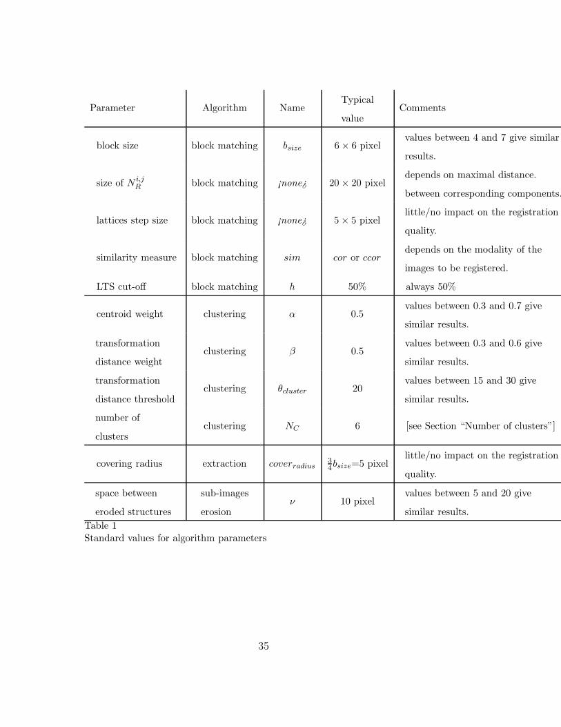
Parameter Algorithm NameTypical

valueComments

block size block matching bsize 6 × 6 pixelvalues between 4 and 7 give similar

results.

size of Ni,jR block matching ¡none¿ 20 × 20 pixel

depends on maximal distance.

between corresponding components.

lattices step size block matching ¡none¿ 5 × 5 pixellittle/no impact on the registration

quality.

similarity measure block matching sim cor or ccordepends on the modality of the

images to be registered.

LTS cut-off block matching h 50% always 50%

centroid weight clustering α 0.5values between 0.3 and 0.7 give

similar results.

transformation

distance weightclustering β 0.5

values between 0.3 and 0.6 give

similar results.

transformation

distance thresholdclustering θcluster 20

values between 15 and 30 give

similar results.

number of

clustersclustering NC 6 [see Section “Number of clusters”]

covering radius extraction coverradius34bsize=5 pixel

little/no impact on the registration

quality.

space between

eroded structures

sub-images

erosionν 10 pixel

values between 5 and 20 give

similar results.

Table 1Standard values for algorithm parameters

35