Numerical method for optimal stopping of piecewise deterministic Markov processes

Submitted to the Annals of Applied Probability

NUMERICAL METHOD FOR OPTIMAL STOPPING OF PIECEWISEDETERMINISTIC MARKOV PROCESSES

By Benoıte de Saporta

Universite de Bordeaux, GREThA, CNRS, UMR 5113,IMB, CNRS, UMR 5251, and INRIA Bordeaux, team CQFD, France

and

By Francois Dufour

Universite de Bordeaux, IMB, CNRS, UMR 5251,and INRIA Bordeaux, team CQFD, France

and

By Karen Gonzalez

Universite de Bordeaux, IMB, CNRS, UMR 5251,and INRIA Bordeaux, team CQFD, France

Abstract We propose a numerical method to approximate thevalue function for the optimal stopping problem of a piecewise deter-ministic Markov process (PDMP). Our approach is based on quan-tization of the post jump location – inter-arrival time Markov chainnaturally embedded in the PDMP, and path-adapted time discretiza-tion grids. It allows us to derive bounds for the convergence rate ofthe algorithm and to provide a computable ε-optimal stopping time.The paper is illustrated by a numerical example.

1. Introduction. The aim of this paper is to propose a computational method for optimalstopping of a piecewise deterministic Markov process X(t) by using a quantization techniquefor an underlying discrete-time Markov chain related to the continuous-time process X(t) andpath-adapted time discretization grids.

Piecewise-deterministic Markov processes (PDMP’s) have been introduced in the literatureby M.H.A. Davis [6] as a general class of stochastic models. PDMP’s are a family of Markov pro-cesses involving deterministic motion punctuated by random jumps. The motion of the PDMPX(t) depends on three local characteristics, namely the flow φ, the jump rate λ and the tran-sition measure Q, which specifies the post-jump location. Starting from x the motion of the

AMS 2000 subject classifications: Primary 93E20; secondary 93E03, 60J25.Keywords and phrases: optimal stopping, piecewise deterministic Markov processes, quantization, numerical

method, dynamic programming

1imsart-aap ver. 2007/12/10 file: QuantifAAP-R.tex date: September 4, 2009

2 B. DE SAPORTA, F. DUFOUR, K.GONZALEZ

process follows the flow φ(x, t) until the first jump time T1 which occurs either spontaneouslyin a Poisson-like fashion with rate λ(φ(x, t)) or when the flow φ(x, t) hits the boundary of thestate-space. In either case the location of the process at the jump time T1: X(T1) = Z1 is selectedby the transition measure Q(φ(x, T1), .). Starting from Z1, we now select the next interjump timeT2 − T1 and postjump location X(T2) = Z2. This gives a piecewise deterministic trajectory forX(t) with jump times Tk and post jump locations Zk which follows the flow φ betweentwo jumps. A suitable choice of the state space and the local characteristics φ, λ, and Q providesstochastic models covering a great number of problems of operations research [6].

Optimal stopping problems have been studied for PDMP’s in [3, 5, 6, 9, 11, 13]. In [11] theauthor defines an operator related to the first jump time of the process, and shows that the valuefunction of the optimal stopping problem is a fixed point for this operator. The basic assumptionin this case is that the final cost function is continuous along trajectories, and it is shown that thevalue function will also have this property. In [9, 13] the authors adopt some stronger continuityassumptions and boundary conditions to show that the value function of the optimal stoppingproblem satisfies some variational inequalities, related to integro-differential equations. In [6],M.H.A. Davis assumes that the value function is bounded and locally Lipschitz along trajectoriesto show that the variational inequalities are necessary and sufficient to characterize the valuefunction of the optimal stopping problem. In [5], the authors weakened the continuity assuptionsof [6, 9, 13]. A paper related to our work is [3] by O.L.V. Costa and M.H.A. Davis. It is the onlyone presenting a computational technique for solving the optimal stopping problem for a PDMPbased on a discretization of the state space similar to the one proposed by H. J. Kushner in [12].In particular, the authors in [3] derive a convergence result for the approximation scheme butno estimation of the rate of convergence is derived.

Quantization methods have been developed recently in numerical probability, nonlinear fil-tering or optimal stochastic control with applications in finance [1, 2, 14, 15, 16, 17]. Morespecifically, powerful and interesting methods have been developed in [1, 2, 17] for computingthe Snell-envelope associated to discrete-time Markov chains and diffusion processes. Roughlyspeaking, the approach developed in [1, 2, 17] for studying the optimal stopping problem fora continuous-time diffusion process Y (t) is based on a time-discretization scheme to obtaina discrete-time Markov chain Y k. It is shown that the original continuous-time optimizationproblem can be converted to an auxiliary optimal stopping problem associated with the discrete-time Markov chain Y k. Under some suitable assumptions, a rate of converge of the auxiliaryvalue function to the original one can be derived. Then, in order to address the optimal stoppingproblem of the discrete-time Markov chain, a twofold computational method is proposed. Thefirst step consists in approximating the Markov chain by a quantized process. There exists anextensive literature on quantization methods for random variables and processes. We do not pre-tend to present here an exhaustive panorama of these methods. However, the interested readermay for instance, consult the following works [10, 14, 17] and references therein. The second

imsart-aap ver. 2007/12/10 file: QuantifAAP-R.tex date: September 4, 2009

OPTIMAL STOPPING FOR PDMP 3

step is to approximate the conditional expectations which are used to compute the backwarddynamic programming formula by the conditional expectation related to the quantized process.This procedure leads to a tractable formula called a quantization tree algorithm (see Proposition4 in [1] or section 4.1 in [17]). Providing the cost function and the Markov kernel are Lipschitz,some bounds and rates of convergence are obtained (see for example section 2.2.2 in [1]).

As regards PDMP’s, it was shown in [11] that the value function of the optimal stoppingproblem can be calculated by iterating a functional operator, labeled L (see equation (3.5) forits definition), which is related to a continuous-time maximization and a discrete-time dynamicprogramming formula. Thus, in order to approximate the value function of the optimal stoppingproblem of a PDMP X(t), a natural approach would have been to follow the same lines as in[1, 2, 17]. However their method cannot be directly applied to our problem for two main reasonsrelated to the specificities of PDMP’s.

First, PDMP’s are in essence discontinuous at random times. Therefore, as pointed out in[11], it will be problematic to convert the original optimization problem into an optimal stop-ping problem associated to a time discretization of X(t) with nice convergence properties.In particular, it appears ill-advised to propose as in [1] a fixed-step time-discretization schemeX(k∆) of the original process X(t). Besides, another important intricacy concerns the tran-sition semigroup Ptt∈R+ of X(t). On the one hand, it cannot be explicitly calculated fromthe local characteristics (φ, λ,Q) of the PDMP (see [4, 7]). Consequently, it will be complicatedto express the Markov kernel P∆ associated to the Markov chain X(k∆). On the other hand,the markov chain X(k∆) is in general not even a Feller chain (see [6, pages 76-77]), thereforeit will be hard to ensure it is K-Lipschitz (see Definition 1 in [1]).

Second, the other main difference stems from the fact the function appearing in the backwarddynamic programming formula associated to L and the reward function g is not continuous evenif some strong regularity assumptions are made on g. Consequently, the approach developedin [1, 2, 17] has to be refined since it can only handle conditional expectations of Lipschitz-continuous functions.

However, by using the special structure of PDMP’s, we are able to overcome both these ob-stacles. Indeed, associated to the PDMP X(t), there exists a natural embedded discrete-timeMarkov chain Θk with Θk = (Zk, Sk) where Sk is given by the inter-arrival time Tk−Tk−1. Themain operator L can be expressed using the chain Θk and a continuous-time maximization.We first convert the continuous-time maximization of operator L into a discrete-time maximiza-tion by using a path-dependent time-discretization scheme. This enables us to approximate thevalue function by the solution of a backward dynamic programming equation in discrete-timeinvolving conditional expectation of the Markov chain Θk. Then, a natural approximation of



this optimization problem is obtained by replacing Θk by its quantized approximation. It mustbe pointed that this optimization problem is related to the calculation of conditional expecta-tions of indicator functions of the Markov chain Θk. As said above, it is not straightforwardto obtain convergence results as in [1, 2, 17]. We deal successfully with indicator functions byshowing that the event on which the discontinuity actually occurs is of small enough probability.This enables us to provide rate of convergence for the approximation scheme.

In addition and more importantly, this numerical approximation scheme enables us to proposea computable stopping rule which also is an ε-optimal stopping time of the original stoppingproblem. Indeed, for any ε > 0 one can construct a stopping time, labeled τ , such that

V (x)− ε ≤ Ex

[g(X(τ))

]≤ V (x)

where V (x) is the optimal value function associated to the original stopping problem. Our com-putational approach is attractive in the sense that it does not require any additional calculations.Moreover, we can characterize how far it is from optimal in terms of the value function. In [1,section 2.2.3, Proposition 6], another criteria for the approximation of the optimal stopping timehas been proposed. In the context of PDMP’s, it must be noticed that an optimal stopping timedoes not generally exists as shown in [11, section 2].

An additional result extends Theorem 1 of U.S. Gugerli [11] by showing that the iteration ofoperator L provides a sequence of random variables which corresponds to a quasi -Snell envelopeassociated to the reward process

g(X(t))

t∈R+

where the horizon time is random and given bythe jump time (Tn)n∈0,...,N of the process

X(t)

t∈R+

.

The paper is organized as follows. In Section 2 we give a precise definition of PDMP’s andstate our notation and assumptions. In Section 3, we state the optimal stopping problem, recalland refine some results from [11]. In Section 4, we build an approximation of the value function.In Section 5, we compute the error between the approximate value function and the real one. InSection 6 we propose a computable ε-optimal stopping time and evaluate its sharpness. Finallyin Section 7 we present a numerical example. Technical results are postponed to the Appendix.

2. Definitions and assumptions. We first give a precise definition of a piecewise de-terministic Markov process. Some general assumptions are presented in the second part of thissection. Let us introduce first some standard notation. Let M be a metric space. B(M) is the setof real-valued, bounded, measurable functions defined on M . The Borel σ-field of M is denoted

by B(M). Let Q be a Markov kernel on (M,B(M)) and w ∈ B(M), Qw(x) =∫Mw(y)Q(x, dy)

for x ∈M . For (a, b) ∈ R2, a ∧ b = min(a, b) and a ∨ b = max(a, b).



2.1. Definition of a PDMP. Let E be an open subset of Rn, ∂E its boundary and E itsclosure. A PDMP is determined by its local characteristics (φ, λ,Q) where:• The flow φ : Rn × R → Rn is a one-parameter group of homeomorphisms: φ is continuous,φ(., t) is an homeomorphism for each t ∈ R satisfying φ(., t+ s) = φ(φ(., s), t)).For all x in E, let us denote

t∗(x) .= inft > 0 : φ(x, t) ∈ ∂E,

with the convention inf ∅ =∞.• The jump rate λ : E → R+ is assumed to be a measurable function satisfying:

(∀x ∈ E), (∃ε > 0) such that∫ ε

0λ(φ(x, s))ds <∞.

• Q is a Markov kernel on (E,B(E)) satisfying the following property:

(∀x ∈ E), Q(x,E − x) = 1.

From these characteristics, it can be shown [6, p. 62-66] that there exists a filtered probabilityspace (Ω,F , Ft, Pxx∈E) such that the motion of the process X(t) starting from a pointx ∈ E may be constructed as follows. Take a random variable T1 such that

Px(T1 > t) .=

e−Λ(x,t) for t < t∗(x)0 for t ≥ t∗(x)

where for x ∈ E and t ∈ [0, t∗(x)]

Λ(x, t) .=∫ t

0λ(φ(x, s))ds.

If T1 generated according to the above probability is equal to infinity, then for t ∈ R+, X(t) =φ(x, t). Otherwise select independently an E-valued random variable (labelled Z1) having dis-tribution Q(φ(x, T1), .), namely Px(Z1 ∈ A) = Q(φ(x, T1), A) for any A ∈ B(E). The trajectoryof X(t) starting at x, for t ≤ T1 , is given by

X(t) .=

φ(x, t) for t < T1,

Z1 for t = T1.

Starting from X(T1) = Z1, we now select the next inter-jump time T2 − T1 and post-jumplocation X(T2) = Z2 is a similar way.

This gives a strong Markov process X(t) with jump timesTkk∈N (where T0 = 0). Asso-

ciated to X(t), there exists a discrete time process(Θn)n∈N defined by Θn = (Zn, Sn) with



Zn = X(Tn) and Sn = Tn−Tn−1 for n ≥ 1 and S0 = 0. Clearly, the process (Θn)n∈N is a Markovchain.

We introduce a standard assumption, see for example equations (24.4) or (24.8) in [6].

Assumption 2.1 For all (x, t) ∈ E × R+, Ex

[∑k

1Tk≤t]<∞.

In particular, it implies that Tk →∞ as k →∞.

For n ∈ N, letMn be the family of all Ft-stopping times which are dominated by Tn and forn < p, letMn,p be the family of all Ft-stopping times ν satisfying Tn ≤ ν ≤ Tp. Let Bc denotethe set of all real-valued, bounded, measurable functions, w defined on E and continuous alongtrajectories up to the jump time horizon: for any x ∈ E, w(φ(x, .)) is continuous on [0, t∗(x)]. LetLc be the set of all real-valued, bounded, measurable functions, w defined on E and Lipschitzalong trajectories:

1. there exists[w]1∈ R+ such that for any (x, y) ∈ E2, u ∈ [0, t∗(x) ∧ t∗(y)], one has∣∣w(φ(x, u))− w(φ(y, u))

∣∣ ≤ [w]1|x− y|,

2. there exists[w]2∈ R+ such that for any x ∈ E, and (t, s) ∈ [0, t∗(x)]2, one has∣∣w(φ(x, t))− w(φ(x, s))

∣∣ ≤ [w]2|t− s|,

3. there exists[w]∗ ∈ R+ such that for any (x, y) ∈ E2, one has∣∣w(φ(x, t∗(x)))− w(φ(y, t∗(y)))

∣∣ ≤ [w]∗|x− y|.In the sequel, for any function f in Bc, we denote by Cf its bound:

Cf = supx∈E|f(x)|,

and for any Lipschitz-continuous function f in B(E) or B(E), we denote by [f ] its Lipschitzconstant: [

f]

= supx6=y∈E

∣∣f(x)− f(y)∣∣

|x− y|.

Remark 2.2 Lc is a subset of Bc and any function in Lc is Lipschitz on E with[w]≤[w]1.

Finally, as a convenient abbreviation, we set for any x ∈ E, λQw(x) = λ(x)Qw(x).



2.2. Assumptions. The following assumptions will be in force throughtout.

Assumption 2.3 The jump rate λ is bounded and there exists[λ]1∈ R+ such for any (x, y) ∈

E2, u ∈ [0, t∗(x) ∧ t∗(y)[, ∣∣λ(φ(x, u))− λ(φ(y, u))∣∣ ≤ [λ]

1|x− y|.

Assumption 2.4 The exit time t∗ is bounded and Lipschitz-continuous on E.

Assumption 2.5 The Markov kernel Q is Lipschitz in the following sense : there exists[Q]∈

R+ such that for any function w ∈ Lc the following two conditions are satisfied:

1. for any (x, y) ∈ E2, u ∈ [0, t∗(x) ∧ t∗(y)], one has∣∣Qw(φ(x, u))−Qw(φ(y, u))∣∣ ≤ [Q][w]

1|x− y|,

2. for any (x, y) ∈ E2, one has∣∣Qw(φ(x, t∗(x)))−Qw(φ(y, t∗(y)))∣∣ ≤ [Q][w]∗|x− y|.

The reward function g associated to the optimal stopping problem satisfies the followinghypothesis.

Assumption 2.6 g is in Lc.

3. Optimal stopping problem. From now on, assume that the distribution of X(0) isgiven by δx0 for a fixed state x0 ∈ E. Let us consider the following optimal stopping problemfor a fixed integer N :

(3.1) supτ∈MN

Ex0 [g(X(τ))]

This problem has been studied by U.S. Gugerli in [11].

Note that Assumption 2.3 yields Λ(x, t) <∞ for all x, t. Hence, for all x in E, the jump timehorizon s∗(x) defined in [11] by t∗(x) ∧ inft ≥ 0, e−Λ(x,t) = 0 is equal to the exit time t∗(x).Therefore, operators H : B(E) → B(E × R+), I : B(E) → B(E × R+), J : B(E) × B(E) →B(E × R+), K : B(E)→ B(E) and L : B(E)×Bc → Bc introduced by Gugerli in [11, section2] reduce to

Hf(x, t) = f(φ(x, t ∧ t∗(x))

)e−Λ(x,t∧t∗(x)),

Iw(x, t) =∫ t∧t∗(x)

0λQw(φ(x, s))e−Λ(x,s)ds,

J(w, f)(x, t) = Iw(x, t) +Hf(x, t),(3.2)

Kw(x) =∫ t∗(x)

0λQw(φ(x, s))e−Λ(x,s)ds+Qw(φ(x, t∗(x)))e−Λ(x,t∗(x)),(3.3)

L(w, h)(x) = supt≥0

J(w, h)(x, t) ∨Kw(x).



It is easy to derive a probabilistic interpretation of operators H, I, K and L in terms of theembedded Markov chain

(Zn, Sn

)n∈N.

Lemma 3.1 For all x ∈ E, w ∈ B(E), f ∈ B(E), h ∈ Bc and t ≥ 0, one has

Hf(x, t) = f(φ(x, t ∧ t∗(x))

)Px(S1 ≥ t ∧ t∗(x)

),

Iw(x, t) = Ex

[w(Z1)1S1<t∧t∗(x)

],

Kw(x) = Ex[w(Z1)

],(3.4)

L(w, h)(x) = supu≤t∗(x)

Ex[w(Z1)1S1<u

]+ h

(φ(x, u)

)Px(S1 ≥ u

)∨Ex

[w(Z1)

].(3.5)

For a reward function g ∈ Bc, it has been shown in [11] that the value function can berecursively constructed by the following procedure:

supτ∈MN

Ex0 [g(X(τ))] = v0(x0)

with vN = g,

vk = L(vk+1, g) for k ≤ N − 1.

Definition 3.2 Introduce the random variables (Vn)n∈0,...,N by

Vn = vn(Zn),

or equivalently

Vn = supu≤t∗(Zn)

E[vn+1(Zn+1)1Sn+1<u + g

(φ(Zn, u)

)1Sn+1≥u

∣∣Zn]∨E

[vn+1(Zn+1)

∣∣Zn].(3.6)

The following result shows that the sequence (Vn)n∈0,...,N corresponds to a quasi -Snell en-velope associated to the reward process

g(X(t))

t∈R+

where the horizon time is random andgiven by the jump times (Tn)n∈0,...,N of the process

X(t)

t∈R+

:

Theorem 3.3 Consider an integer n < N . Then

Vn = supν∈Mn,N

Ex0 [g(X(ν))|FTn ].



Proof: Let ν ∈ Mn,N . According to Proposition B.4 and Corollary B.6 in Appendix B, thereexists ν : E × (R+ × E)n × Ω → R+ such that for all (z0, γ) ∈ E × (R+ × E)n the mappingν(z0, γ) : Ω → R+ is an

Ftt∈R+

-stopping time satisfying ν(z0, γ) ≤ TN−n, and ν = Tn +ν(Z0,Γn, θTn), where Γn =

(S1, Z1, . . . , Sn, Zn

)and θ is the shift operator. For (z0, γ) ∈ E ×

(R+ × E)n define W : E × (R+ × E)n → R by

W(z0, γ) = Ezn [g(X(ν(z0, γ)))] ≤ supτ∈MN−n

EZn [g(X(τ))],

where γ = (s1, z1, . . . , sn, zn). Hence, the strong Markov property of the process X(t) yields

Ex0 [g(X(ν))|FTn ] = Ex0 [g(X(Tn + ν(Z0,Γn, θTn)))|FTn ] =W(Z0,Γn).

Consequently, one has

Ex0 [g(X(ν))|FTn ] ≤ supτ∈MN−n

EZn [g(X(τ))],

and therefore, one has

supν∈Mn,N

Ex0 [g(X(ν))|FTn ] ≤ supτ∈MN−n

EZn [g(X(τ))],(3.7)

Conversely, consider τ ∈ MN−n. It is easy to show that Tn + τ θTn ∈ Mn,N . The strongMarkov property of the process X(t) again yields

EZn [g(X(τ))] = Ex0 [g(X(Tn + τ θTn))|FTn ] ≤ supν∈Mn,N

Ex0 [g(X(ν))|FTn ],

hence we obtain

supτ∈MN−n

EZn [g(X(τ))] ≤ supν∈Mn,N

Ex0 [g(X(ν))|FTn ].(3.8)

Conbining equations (3.7) and (3.8), one has

supτ∈MN−n

EZn [g(X(τ))] = supν∈Mn,N

Ex0 [g(X(ν))|FTn ].

Finally, it is proved in [11, Theorem 1] that vn(x) = supτ∈MN−n Ex[g(X(τ))], whence

Vn = supτ∈MN−n

EZn [g(X(τ))],

showing the result. 2



4. Approximation of the value function. To approximate the sequence of value func-tions (Vn), we proceed in two steps. First, the continuous-time maximization of operator Lis converted into a discrete-time maximization by using a path-dependent time-discretizationscheme to give a new operator Ld. In particular, it is important to remark that these time-discretization grids depend on the the post-jump locations Zk of the PDMP (see Definition4.1 and Remark 4.2). Second, the conditional expectations of the Markov chain (Θk) in the def-inition of Ld are replaced by the conditional expectations of its quantized approximation (Θk)to define an operator Ld.

First, we define the path-adapted discretization grids as follows.

Definition 4.1 For z ∈ E, set ∆(z) ∈]0, t∗(z)[. Define n(z) = int( t∗(z)

∆(z)

)− 1, where int(x)

denotes the greatest integer smaller than or equal to x. The set of points (ti)i∈0,...,n(z) withti = i∆(z) is denoted by G(z). This is the grid associated to the time interval [0, t∗(z)].

Remark 4.2 It is important to note that, for all z ∈ E, not only one has t∗(z) /∈ G(z), but alsomaxG(z) = tn(z) ≤ t∗(z)−∆(z). This property is crucial for the sequel.

Definition 4.3 Consider for w ∈ B(E) and z ∈ E,

Ld(w, g)(z) = maxs∈G(z)

E[w(Z1)1S1<s + g

(φ(z, s)

)1S1≥s

∣∣Z0 = z]

∨E[w(Z1)

∣∣Z0 = z]

Now let us turn to the quantization of (Θn). The quantization algorithm will provide us witha finite grid ΓΘ

n ⊂ E × R+ at each time 0 ≤ n ≤ N as well as weights for each point of thegrid, see e.g. [1, 14, 17]. Set p ≥ 1 such that Θn has finite moments at least up to the order pand let pn be the closest-neighbour projection from E × R+ onto ΓΘ

n (for the distance of normp; if there are several equally close neighbours, pick the one with the smallest index). Then thequantization of Θn is defined by

Θn =(Zn, Sn

)= pn

(Zn, Sn

).

We will also denote ΓZn the projection of ΓΘn on E and ΓSn the projection of ΓΘ

n on R+.

In practice, one will first compute the quantization grids and weights, and then compute apath-adapted time-grid for each z ∈ ΓZn , for all 0 ≤ n ≤ N − 1. Hence, there is only a finitenumber time grids to compute, and like the quantization grids, they can be computed and storedoff-line.

The definition of the discretized operators now naturally follows the characterization given inLemma 3.1.



Definition 4.4 For k ∈ 1, . . . , N, w ∈ B(ΓZk ), z ∈ ΓZk−1, and s ∈ R+

Jk(w, g)(z, s) = E[w(Zk)1Sk<s + g

(φ(z, s)

)1Sk≥s

∣∣Zk−1 = z]

Kk(w)(z) = E[w(Zk)

∣∣Zk−1 = z]

Ldk(w, g)(z) = maxs∈G(z)

Jk(w, g)(z, s)

∨ Kk(w)(z).

Note that Θn is a random variable taking finitely many values, hence the expectations aboveactually are finite sums, the probability of each atom being given by its weight on the quanti-zation grid. We can now give the complete contruction of the sequence approximating (Vn).

Definition 4.5 Consider vN (z) = g(z) where z ∈ ΓZN and for k ∈ 1, . . . , N

vk−1(z) = Ldk(vk, g)(z),(4.1)

where z ∈ ΓZk−1

Definition 4.6 The approximation of Vk is denoted by

Vk = vk(Zk),(4.2)

for k ∈ 0, . . . , N.

5. Error estimation for the value function. We are now able to state our main result,namely the convergence of our approximation scheme with an upper bound for the rate ofconvergence.

Theorem 5.1 Set n ∈ 0, . . . , N − 1, and suppose that ∆(z), for z ∈ Γzn, are chosen such that

minz∈Γzn∆(z) > (2Cλ)−1/2([t∗]‖Zn − Zn‖p + ‖Sn+1 − Sn+1‖p

)1/2.

Then the discretization error for Vn is no greater than the following:

‖Vn − Vn‖p ≤∥∥Vn+1 − Vn+1

∥∥p

+ α‖∆(Zn)‖p + βn‖Zn − Zn‖p + 2[vn+1

]‖Zn+1 − Zn+1‖p

+γ([t∗]‖Zn − Zn‖p + ‖Sn+1 − Sn+1‖p

)1/2,

where α =[g]2

+ 2CgCλ, βn =[vn]

+[vn+1

]1E2 + CgE4 +

([g]1

+[g]2

[t∗])∨([vn+1

]∗[Q])

,γ = 4Cg(2Cλ)1/2, and E2 and E4 are defined in Appendix A.

Recall that VN = g(ZN ) and VN = g(ZN ), hence ‖VN − VN‖p ≤ [g]∥∥ZN − ZN∥∥p. In addition,

the quantization error ‖Θn − Θn‖p goes to zero as the number of points in the grids goes toinfinity, see e.g. [14]. Hence |V0− V0| can be made arbitrarily small by an adequate choice of thediscretizations parameters.



Remark that the squere root in the last error term is the price to pay for integrating non-continuous functions, see the definition of operator J with the indicator functions, and theintroduction of section 5.2.

To prove Theorem 5.1, we split the left-hand-side difference into four terms:

‖Vn − Vn‖p ≤4∑i=1

Ξi,

where

Ξ1 = ‖vn(Zn)− vn(Zn)‖pΞ2 = ‖L(vn+1, g)(Zn)− Ld(vn+1, g)(Zn)‖pΞ3 = ‖Ld(vn+1, g)(Zn)− Ldn+1(vn+1, g)(Zn)‖pΞ4 = ‖Ldn+1(vn+1, g)(Zn)− Ldn+1(vn+1, g)(Zn)‖p.

The first term is easy enough to handle thanks to Proposition A.7 in Appendix A.2.

Lemma 5.2 A upper bound for Ξ1 is

‖vn(Zn)− vn(Zn)‖p ≤ [vn]‖Zn − Zn‖p.

We are going to study the other terms one by one in the following sections.

5.1. Second term. In this part we study the error induced by the replacement of the supre-mum over all non-negative t smaller than or equal to t∗(z) by the maximum over the finite gridG(z) in the definition of operator L.

Lemma 5.3 Let w ∈ Lc. Then for all z ∈ E,∣∣ supt≤t∗(z)

J(w, g)(z, t)− maxs∈G(z)

J(w, g)(z, s)∣∣ ≤ (CwCλ +

[g]2

+ CgCλ)∆(z).

Proof: Clearly, there exists t ∈ [0, t∗(z)] such that supt≤t∗(z) J(w, g)(z, t) = J(w, g)(z, t), andthere exists 0 ≤ i ≤ n(z) such that t ∈ [ti, ti+1] (with tn(z)+1 = t∗(z)). Consequently, Lemma A.2yields

0 ≤ supt≤t∗(z)

J(w, g)(z, t)− maxs∈G(z)

J(w, g)(z, s) ≤ J(w, g)(z, t)− J(w, g)(z, ti)

≤(CwCλ +

[g]2

+ CgCλ)|t− ti|

≤(CwCλ +

[g]2

+ CgCλ)|ti+1 − ti|,

implying the result. 2

Turning back to the second error term, one gets the following bound.



Lemma 5.4 A upper bound for Ξ2 is

‖L(vn+1, g)(Zn)− Ld(vn+1, g)(Zn)‖p ≤([g]2

+ 2CgCλ)‖∆(Zn)‖p.

Proof: From the definition of L and Ld we readily obtain

‖L(vn+1, g)(Zn)− Ld(vn+1, g)(Zn)‖p≤∥∥ supt≤t∗(Zn)

J(vn+1, g)(Zn, t)− maxs∈G(Zn)

J(vn+1, g)(Zn, s)∥∥p.

Now in view of the previous lemma, one has

‖L(vn+1, g)(Zn)− Ld(vn+1, g)(Zn)‖p≤(Cvn+1Cλ +

[g]2

+ CgCλ)‖∆(Zn)‖p.

Finaly, note that Cvn+1 = Cg (see Appendix A.2), completing the proof. 2

5.2. Third term. This is the crucial part of our derivation, where we need to compare condi-tional expectations relative to the real Markov chain (Zn, Sn) and its quantized approximation(Zn, Sn). The main difficulty stems from the fact that some functions inside the expectations areindicator functions and in particular they are not Lipschitz-continuous. We manage to overcomethis difficulty by proving that the event on which the discontinuity actually occurs is of smallenough probability, this is the aim of the following two lemmas.

Lemma 5.5 For all n ∈ 0, . . . , N − 1 and 0 < η < minz∈ΓZn

∆(z),

∥∥∥ maxs∈G(Zn)

E[|1Sn+1<s − 1Sn+1<s

|∣∣Zn]∥∥∥

p≤ 1

η‖Sn+1 − Sn+1‖p + 2Cλη.

Proof: Set 0 < η < minz∈ΓZn

∆(z). Remark that the difference of indicator functions is non-zero

if and only if Sn+1 and Sn+1 are on either side of s. Hence, one has∣∣1Sn+1<s − 1Sn+1<s∣∣ ≤ 1|Sn+1−Sn+1|>η

+ 1|Sn+1−s|≤η.

This yields ∥∥ maxs∈G(Zn)

E[|1Sn+1<s − 1Sn+1<s

|∣∣Zn]∥∥p

≤∥∥1|Sn+1−Sn+1|>η

∥∥p

+∥∥ maxs∈G(Zn)

E[1s−η≤Sn+1≤s+η

∣∣Zn]∥∥p.(5.1)

On the one hand, Chebychev’s inequality yields

(5.2)∥∥1|Sn+1−Sn+1|>η

∥∥pp

= P(|Sn+1 − Sn+1| > η) ≤

∥∥Sn+1 − Sn+1

∥∥pp

ηp.



On the other hand, as s ∈ G(Zn) and by definition of η, one has s+η < t∗(Zn), see Remark 4.2.Thus, one has

E[1s−η≤Sn+1≤s+η

∣∣Zn] = E[E[1s−η≤Sn+1≤s+η|Zn = Zn

]∣∣∣Zn]= E

[ ∫ s+η

s−ηλ(φ(Zn, u))du

∣∣∣Zn]≤ 2ηCλ.(5.3)

Combining equations (5.1)-(5.3), the result follows. 2

Lemma 5.6 For all n ∈ 0, . . . , N and 0 < η < minz∈ΓZn

∆(z),

∥∥1t∗(Zn)<t∗(Zn)−η

∥∥p≤ [t∗]‖Zn − Zn‖p

η.

Proof: We use Chebychev’s inequality again. One clearly has

E[|1t∗(Zn)<t∗(Zn)−η|

p]

= P(t∗(Zn) < t∗(Zn)− η

)≤ P

(∣∣t∗(Zk)− t∗(Zk)∣∣ > η)≤

[t∗]p‖Zk − Zk‖ppηp

,

showing the result. 2

Now we turn to the consequences of replacing the Markov chain (Zn, Sn) by its quantizedapproximation (Zn, Sn) in the conditional expectations.

Lemma 5.7 Let w ∈ Lc, then one has∣∣∣E[w(Zn+1)∣∣Zn = Zn

]−E

[w(Zn+1)

∣∣Zn]∣∣∣≤(CwE4 +

[w]1E2 +

[w]∗[Q])

E[|Zn − Zn|

∣∣ Zn]+[w]E[|Zn+1 − Zn+1|

∣∣Zn].Proof: First, note that

E[w(Zn+1)

∣∣Zn = Zn]−E

[w(Zn+1)

∣∣Zn] = E[w(Zn+1)

∣∣Zn = Zn]−E

[w(Zn+1)

∣∣Zn]+ E

[w(Zn+1)

∣∣Zn]−E[w(Zn+1)

∣∣Zn].On the one hand, Remark 2.2 yields∣∣∣E[w(Zn+1)

∣∣Zn]−E[w(Zn+1)

∣∣Zn]∣∣∣ ≤ [w]E[|Zn+1 − Zn+1|∣∣Zn].



On the other hand, recall that by construction of the quantized process, one has(Zn, Sn

)=

pn(Zn, Sn

). Hence we have the following property: σZn ⊂ σZn, Sn. By using the special

structure of the PDMP X(t), we have σZn, Sn ⊂ FTn . Now, by using the Markov propertyof the process X(t), it follows

E[w(Zn+1)

∣∣Zn] = E[E[w(Zn+1)

∣∣FTn]∣∣∣Zn] = E[E[w(Zn+1)

∣∣Zn]∣∣∣Zn].Equation (3.4) thus yields

E[w(Zn+1)

∣∣Zn = Zn]−E

[w(Zn+1)

∣∣Zn]= E

[E[w(Zn+1)

∣∣Zn = Zn]−E

[w(Zn+1)

∣∣Zn]∣∣∣Zn]= E

[Kw(Zn)−Kw(Zn)

∣∣∣Zn].Now we use Lemma A.4 to conclude. 2

Now we combine the preceding lemmas to derive the third error term.

Lemma 5.8 For all 0 < η < minz∈ΓZn

∆(z), an upper bound for Ξ3 is

∥∥Ld(vn+1, g)(Zn)− Ldn+1(vn+1, g)(Zn)∥∥p

≤[vn+1

]1E2 + CgE4 + 2Cg

[t∗]

η+([g]1

+[g]2

[t∗])∨([vn+1

]∗[Q])‖Zn − Zn‖p

+[vn+1

]‖Zn+1 − Zn+1‖p + 2Cg

(2Cλη +

‖Sn+1 − Sn+1‖pη

).

Proof: To simplify notation, set Ψ(x, y, t) = vn+1(y)1t<s+g(φ(x, t)

)1t≥s. From the definition

of Ld and Ldn+1, one readily obtains∣∣Ld(vn+1, g)(Zn)−Ldn+1(vn+1, g)(Zn)∣∣

≤ maxs∈G(Zn)

∣∣∣E[Ψ(Zn, Zn+1, Sn+1)∣∣Zn = Zn

]−E

[Ψ(Zn, Zn+1, Sn+1)

∣∣Zn]∣∣∣∨∣∣∣E[vn+1(Zn+1)

∣∣Zn = Zn]−E

[vn+1(Zn+1)

∣∣Zn]∣∣∣.(5.4)

On the one hand, combining Lemma 5.7 and the fact that vn+1 is in Lc (see Proposition A.7),we obtain ∣∣∣E[vn+1(Zn+1)

∣∣Zn = Zn]−E

[vn+1(Zn+1)

∣∣Zn]∣∣∣≤

[vn+1

]E[|Zn+1 − Zn+1

∣∣ Zn]+(CgE4 +

[vn+1

]1E2 +

[vn+1

]∗[Q])

E[|Zn − Zn|

∣∣ Zn].(5.5)



On the other hand, similar arguments as in the proof of Lemma 5.7 yield

E[Ψ(Zn, Zn+1, Sn+1)

∣∣Zn = Zn]−E

[Ψ(Zn, Zn+1, Sn+1)

∣∣Zn]= E

[E[Ψ(Zn, Zn+1, Sn+1)

∣∣Zn = Zn]−E

[Ψ(Zn, Zn+1, Sn+1)

∣∣Zn = Zn]∣∣∣Zn]

+E[Ψ(Zn, Zn+1, Sn+1)

∣∣Zn]−E[Ψ(Zn, Zn+1, Sn+1)

∣∣Zn].(5.6)= Υ1 + Υ2

The second difference of the right hand side of equation (5.6), labeled Υ2, clearly satisfies

|Υ2| ≤[vn+1

]E[|Zn+1 − Zn+1|

∣∣Zn]+[g]1E[|Zn − Zn|

∣∣Zn]+2CgE

[|1Sn+1<s − 1Sn+1<s

|∣∣Zn].(5.7)

Let us turn now to the first difference of the right hand side of equation (5.6), labeled Υ1. Wemeet another difficulty here. Indeed, we know by construction that s < t∗(Zn), but we knownothing regarding the relative positions of s and t∗(Zn). On the event where s ≤ t∗(Zn) as well,we recognize operator J inside the expectations. On the opposite event s > t∗(Zn), we crudelybound Ψ by Cvn+1 + Cg = 2Cg. Hence, one obtains

|Υ1| ≤ E[∣∣J(vn+1, g)(Zn, s)− J(vn+1, g)(Zn, s)

∣∣1s≤t∗(Zn)

∣∣∣Zn]+ 2CgE[1t∗(Zn)<s

∣∣Zn].Now Lemma A.3 gives an upper bound for the first term. As for the indicatror function, bydefinition of G(Zn) and our choice of η, we have s < t∗(Zn)− η. Thus, one has

|Υ1| ≤(CgE1 +

[vn+1

]1E2 + E3

)E[|Zn − Zn|

∣∣Zn]+ 2CgE[1t∗(Zn)<t∗(Zn)−η

∣∣Zn].(5.8)

Now, combining (5.4), (5.5), (5.7) and (5.8), and the fact that CgE1+E3 = CgE4+[g]1+[g]2

[t∗],

one gets∣∣Ld(vn+1,g)(Zn)− Ldn+1(vn+1, g)(Zn)∣∣

≤[vn+1

]1E2 + CgE4 +

([g]1

+[g]2

[t∗])∨([vn+1

]∗[Q])

E[|Zn − Zn|

∣∣Zn]+[vn+1

]E[|Zn+1 − Zn+1|

∣∣Zn]+ 2CgE

[1t∗(Zn)<t∗(Zn)−η

∣∣Zn]+ 2Cg maxs∈G(Zn)

E[|1Sn+1<s − 1Sn+1<s

|∣∣Zn].

Finally, we conclude by taking the Lp norm on both sides and using Lemmas 5.5 and 5.6. 2

5.3. Fourth term. The last error term is a mere comparison of two finite sums.

Lemma 5.9 An upper bound for Ξ4 is

‖Ldn+1(vn+1, g)(Zn)− Ldn+1(vn+1, g)(Zn)‖p ≤[vn+1

]∥∥Zn+1 − Zn+1

∥∥p

+∥∥Vn+1 − Vn+1

∥∥p.



Proof: By definition of operator Ldn, one has

‖Ldn+1(vn+1, g)(Zn)− Ldn+1(vn+1, g)(Zn)‖p=

∥∥∥ maxs∈G(Zn)

E[vn+1(Zn+1)1Sn+1<s

+ g(φ(Zn, s)

)1Sn+1≥s

∣∣Zn] ∨ E[vn+1(Zn+1)

∣∣Zn]− maxs∈G(Zn)

E[vn+1(Zn+1)1Sn+1<s

+ g(φ(Zn, s)

)1Sn+1≥s

∣∣Zn] ∨ E[vn+1(Zn+1)

∣∣Zn]∥∥∥p

≤∥∥E[vn+1(Zn+1)− vn+1(Zn+1)

∣∣Zn]∥∥p

≤∥∥vn+1(Zn+1)− vn+1(Zn+1)

∥∥p

+∥∥vn+1(Zn+1)− vn+1(Zn+1)

∥∥p.

We conclude using the fact that vn+1 ∈ Lc (see Proposition A.7) and the definitions of Vn andVn. 2

5.4. Proof of Theorem 5.1. We can finally turn to the proof of Theorem 5.1. Lemmas 5.2,5.4, 5.8 and 5.9 from the preceding sections directly yield, for all 0 < η < min

z∈Γzn∆(z),

‖Vn − Vn‖p ≤[vn]‖Zn − Zn‖p +

([g]2

+ 2CgCλ)‖∆(Zn)‖p

+[vn+1

]1E2 + CgE4 + 2Cg

[t∗]

η+([g]1

+[g]2

[t∗])∨([vn+1

]∗[Q])‖Zn − Zn‖p

+[vn+1

]‖Zn+1 − Zn+1‖p + 2Cg

(2Cλη +

‖Sn+1 − Sn+1‖pη

)+[vn+1

]∥∥Zn+1 − Zn+1

∥∥p

+∥∥Vn+1 − Vn+1

∥∥p.

The optimal choice for η clearly satisfies

2Cλη =1η

([t∗]‖Zn − Zn‖p + ‖Sn+1 − Sn+1‖p

),

providing it also satisfies the condition 0 < η < minz∈Γzn∆(z). Hence, rearranging the terms above,

one gets the expected result:

‖Vn − Vn‖p ≤∥∥Vn+1 − Vn+1

∥∥p

+([g]2

+ 2CgCλ)‖∆(Zn)‖p

+[vn]

+[vn+1

]1E2 + CgE4 +

([g]1

+[g]2

[t∗])∨([vn+1

]∗[Q])‖Zn − Zn‖p

+ 2[vn+1

]‖Zn+1 − Zn+1‖p + 4Cg(2Cλ)1/2([t∗]‖Zn − Zn‖p + ‖Sn+1 − Sn+1‖p

)1/2.

6. Numerical construction of an ε-optimal stopping time. In [11, Theorem 1], U.S.Gugerli defined an ε-optimal stopping time for the original problem. Roughly speaking, thisstopping time depends on the embedded Markov chain (Θn), and on the optimal value function.



Therefore, a natural candidate for an ε-optimal stopping time should be obtained by replacing theMarkov chain (Θn) and the optimal value function by their quantized approximations. However,this leads to un-tractable comparisons between some quantities involving (Θn) and its quantizedapproximation. It is then far from obvious to show that this method would provide a computableε-optimal stopping rule. Nonetheless, by modifying the approach of U.S. Gugerli [11], we areable to propose a numerical construction of an ε-optimal stopping time of the original stoppingproblem.

Here is how we proceed. First, recall that pn be the closest-neighbour projection from E×R+

onto ΓΘn , and for all (z, s) ∈ E × R+ define (zn, sn) = pn(z, s). Note that zn and sn depend on

both z and s. Now, for n ∈ 1, . . . , N, define

s∗n(z, s) = mint ∈ G(zn−1)

∣∣∣Jn(vn, g)(zn−1, t) = maxu∈G(zn−1)

Jn(vn, g)(zn−1, u)

and

rn,β(z, s) =

t∗(z) if Knvn(zn−1) > max

u∈G(zn−1)Jn(vn, g)(zn−1, u),

s∗n(z, s)1s∗n(z,s)<t∗(z) + (t∗(z)− β)1s∗(z,s)≥t∗(z) otherwise.

Note the use of both the real jump time horizon t∗(z) and the quantized approximations of K,J and (z, s). Set

τ1 = rN,β(Z0, S0) ∧ T1,

and for n ∈ 1, . . . , N − 1, set

τn+1 =

rN−n,β(Z0, S0) if T1 > rN−n,β(Z0, S0),T1 + τn θT1 otherwise.

Our stopping rule is then defined by τN .

Remark 6.1 This procedure is especially appealing because it requires no more calculation: wehave already computed the values of Kn and Jn on the grids. One just has to store the pointwhere the maximum of Jn is reached.

Lemma 6.2 τN is an FT -stopping time.

Proof: Set U1 = r1,β(Z0, S0) and for 2 ≤ k ≤ N Uk = rk,β(Zk−1, Sk−1)1rk−1,β(Zk−2,Sk−2)≥Sk−1.

One then clearly has τN =N∑k=1

Uk ∧ Sk which is an FT -stopping time by Proposition B.5. 2



Now let us show that this stopping time provides a good approximation of the value functionV0. Namely, for all z ∈ E set

vn(z) = E[g(XτN−n)

∣∣Zn = z],

and in accordance to our previous notation introduce, for n ∈ 1, . . . , N − 1

V n = vn(Zn).

The comparison between V0 and V 0 is provided by the next two Theorems.

Theorem 6.3 Set n ∈ 0, . . . , N − 2 and suppose the discretization parameters are chosensuch that there exists 0 < a < 1 satisfying

β

a= (2Cλ)−1/2

( [t∗]1− a

‖Zn − Zn‖p + ‖Sn+1 − Sn+1‖p)1/2

< minz∈Γzn∆(z).

Then one has∥∥V n − Vn∥∥p≤

∥∥V n+1 − Vn+1

∥∥p

+∥∥Vn+1 − Vn+1

∥∥p

+∥∥Vn − Vn∥∥p

+2[vn+1

]∥∥Zn+1 − Zn+1

∥∥p

+ an∥∥Zn − Zn∥∥p

+4Cg(2Cλ)1/2( [t∗]

1− a‖Zn − Zn‖p + ‖Sn+1 − Sn+1‖p

)1/2,

with an =(2[vn+1

]1E2 + 2CgCt∗

[λ]1(2 + Ct∗Cλ) +

(4CgCλ

[t∗]

+ 2[vn+1

]∗[Q])∨ (3

[g]1))

.

Proof: The definition of τn and the strong Markov property of the process X(t) yield

vn(Zn)= E

[g(Xrn+1,β(Zn,Sn))1Sn+1>rn+1,β(Zn,Sn)

∣∣Zn]+ E[vn+1(Zn+1)1Sn+1≤rn+1,β(Zn,Sn)

∣∣Zn]= 1rn+1,β(Zn,Sn)≥t∗(Zn)Kvn+1(Zn) + 1rn+1,β(Zn,Sn)<t∗(Zn)J(vn+1, g)(Zn, rn+1,β(Zn, Sn)).

However, our definition of rn,β with the special use of parameter β impliesrn+1,β(Zn, Sn) ≥ t∗(Zn)

=Kn+1vn+1(Zn) > max

s∈G(Zn)

Jn+1(vn+1, g)(Zn, s).

Consequently, one obtains

vn(Zn) = Kn+1vn+1(Zn) ∨ maxs∈G(Zn)

Jn+1(vn+1, g)(Zn, s)

+ 1rn+1,β(Zn,Sn)≥t∗(Zn)[Kvn+1(Zn)− Kn+1vn+1(Zn)

](6.1)

+ 1rn+1,β(Zn,Sn)<t∗(Zn)[J(vn+1, g)(Zn, rn+1,β(Zn, Sn))− max

s∈G(Zn)

Jn+1(vn+1, g)(Zn, s)].



Let us study the term with operator K. First, we insert Vn to be able to use our work of theprevious section (we cannot directy apply it to vn because it may not be Lipschitz-continuous).Clearly, one has∣∣∣Kvn+1(Zn)− Kn+1vn+1(Zn)

∣∣∣ ≤ E[|V n+1 − Vn+1|

∣∣Zn]+∣∣∣Kvn+1(Zn)− Kn+1vn+1(Zn)

∣∣∣.(6.2)

Similar calculations to those of Lemmas A.4, 5.7 and 5.9, and Equation (5.5) yield∣∣∣Kvn+1(Zn)− Kn+1vn+1(Zn)∣∣∣

≤(CgE4 +

[vn+1

]1E2 +

[vn+1

]∗[Q])(∣∣Zn − Zn∣∣+ E

[|Zn − Zn|

∣∣Zn])+2[vn+1

]E[|Zn+1 − Zn+1|

∣∣Zn]+ E[|Vn+1 − Vn+1|

∣∣Zn].(6.3)

Now we turn to operator J . Set Rn = rn+1,β(Zn, Sn). We first study the case when Rn =s∗n+1(Zn, Sn) < t∗(Zn). By definition, one has

Jn+1(vn+1, g)(Zn, Rn) = maxs∈G(Zn)

Jn+1(vn+1, g)(Zn, s).

As above, we insert Vn and obtain∣∣∣[J(vn+1, g)(Zn, Rn)− maxs∈G(Zn)

Jn+1(vn+1, g)(Zn, s)]1Rn=s∗n+1(Zn,Sn)

∣∣∣≤ E

[|V n+1 − Vn+1|

∣∣Zn]1Rn=s∗n+1(Zn,Sn)

+∣∣∣J(vn+1, g)(Zn, Rn)− Jn+1(vn+1, g)(Zn, Rn))

∣∣∣1Rn=s∗n+1(Zn,Sn).(6.4)

Again, similar arguments as those used for Lemmas A.3, 5.6 and 5.9, and Equations (5.6), (5.7)and (5.8) yield, on Rn = s∗n+1(Zn, Sn)∣∣∣J(vn+1, g)(Zn, Rn)− Jn+1(vn+1, g)(Zn, Rn))

∣∣∣≤

([vn+1

]1E2 +

[g]1

+ CgCt∗[λ]1(2 + Ct∗Cλ))

(∣∣Zn − Zn∣∣+ E[|Zn − Zn|

∣∣Zn])+2[vn+1

]E[|Zn+1 − Zn+1|

∣∣Zn]+ E[|Vn+1 − Vn+1|

∣∣Zn]+[g]1E[|Zn − Zn|

∣∣Zn]+ 2CgE[|1Sn+1<Rn − 1Sn+1<Rn

|∣∣Zn].(6.5)

Note that all the constants with a factor[t∗]

have vanished, because we know here that bothRn < t∗(Zn) and Rn < t∗(Zn) hold on Rn = s∗n+1(Zn, Sn).



Finally, on s∗(Zn) ≥ t∗(Zn) = Rn + β, by construction of the grid G(Zn) (see Remark 4.2),one has for all 0 < η < min

z∈ΓZn

∆(z),

Rn = t∗(Zn)− β < s∗(Zn) < t∗(Zn)− η.

Consequently, using the crude bound∣∣∣J(vn+1, g)(Zn, Rn))∣∣∣+ ∣∣∣ max

s∈G(Zn)

Jn+1(vn+1, g)(Zn, s)∣∣∣ ≤ 2Cg,

one obtains∣∣∣J(vn+1, g)(Zn, rn+1,β(Zn, Sn))− maxs∈G(Zn)

Jn+1(vn+1, g)(Zn, s)∣∣∣1rn+1,β(Zn,Sn)=t∗(Zn)−β

≤ 2Cg∣∣∣1t∗(Zn)−β<t∗(Zn)−η

∣∣∣.(6.6)

Now the combination of Equations (6.1)-(6.6) and Lemmas 5.5 and 5.6 yields, for all β < η <minz∈ΓZn

∆(z)

∥∥V n − Vn∥∥p≤

∥∥V n+1 − Vn+1

∥∥p

+∥∥Vn+1 − Vn+1

∥∥p

+ 2[vn+1

]∥∥Zn+1 − Zn+1

∥∥p

+∥∥Zn − Zn∥∥p(2

[vn+1

]1E2 + 2CgCt∗

[λ]1(2 + Ct∗Cλ)

+(4CgCλ

[t∗]

+ 2[vn+1

]∗[Q])∨ (3

[g]1))

+2Cg(2Cλη +

1η

∥∥Sn+1 − Sn+1

∥∥p

+[t∗]

η − β∥∥Zn − Zn∥∥p).

Now suppose there exists 0 < a < 1 such that η = a−1β. Then the optimal choice for η satisfies

2Cλη =1η

( [t∗]1− a

‖Zn − Zn‖p + ‖Sn+1 − Sn+1‖p),

providing it also satisfies the condition 0 < η < minz∈Γzn∆(z), Hence the result. 2

Theroem 6.3 gives a recursive error estimation. Here is the initializing step.

Theorem 6.4 Suppose the discretization parameters are chosen such that there exists 0 < a < 1satisfying

β

a= (2Cλ)−1/2

( [t∗]1− a

‖ZN−1 − ZN−1‖p + ‖SN − SN‖p)1/2

< minz∈ΓzN−1

∆(z).



Then one has∥∥V N−1 − VN−1

∥∥p≤

∥∥VN−1 − VN−1

∥∥p

+ 3[g]∥∥ZN − ZN∥∥p + aN−1

∥∥ZN−1 − ZN−1

∥∥p

+4Cg(2Cλ)1/2( [t∗]

1− a‖ZN−1 − ZN−1‖p + ‖SN − SN‖p

)1/2,

with aN−1 =(2[g]1E2 + 2CgCt∗

[λ]1(2 + Ct∗Cλ) +

(4CgCλ

[t∗]

+ 2[g]∗[Q])∨ (3

[g]1))

.

Proof: As before, the strong Markov property of the process X(t) yields

vN−1(ZN−1) = E[g(XrN,β(ZN−1,SN−1))1SN>rN,β(ZN−1,SN−1)

∣∣ZN−1

]+ E

[g(ZN )1SN≤rN,β(ZN−1,SN−1)

∣∣ZN−1

]= 1rN,β(ZN−1,SN−1)≥t∗(ZN−1)Kg(ZN−1)

+ 1rN,β(ZN−1,SN−1)<t∗(ZN−1)J(g, g)(ZN−1, rN,β(ZN−1, SN−1)).

The rest of the proof is similar to that of the previous theorem. 2

As in Section 5, it is now clear that an adequate choice of discretization parameters yieldsarbitrarily small errors if one uses the stopping-time τN .

7. Example. Now we apply the procedures decribed in Sections 4 and 6 on a simple PDMPand present numerical results.

Set E = [0, 1[, and ∂E = 1. The flow is defined on [0, 1] by φ(x, t) = x+vt for some positivev, the jump rate is defined on [0, 1] by λ(x) = βxα, with β > 0 and α ≥ 1, and for all x ∈ [0, 1],one sets Q(x, ·) to be the uniform law on [0, 1/2]. Thus, the process moves with constant speed vtowards 1, but the closer it gets to the boundary 1, the higher the probability to jump backwardson [0, 1/2]. Figure 1 shows two trajectories of this process for x0 = 0, v = α = 1 and β = 3 andup to the 10-th jump.

The reward function g is defined on [0, 1] by g(x) = x. Our assumptions are clearly satisfied,and we are even in the special case when the flow is Lipschitz-continuous (see Remark A.8). Allthe constants involved in Theorems 5.1 and 6.3 can be computed explicitely.

The real value function V0 = v0(x0) is unknown, but, as our stopping rule τN is a stoppingtime dominated by TN , one clearly has

(7.1) V 0 = Ex0

[g(X(τN )

)]≤ V0 = sup

τ∈MN

Ex0

[g(X(τ))

]≤ Ex0

[sup

0≤t≤TNg(X(t)

)].

The first and last terms can be evaluated by Monte Carlo simulations, which provides anotherindicator of the sharpness of our numerical procedure. For 106 Monte Carlo simulations, oneobtains Ex0

[sup0≤t≤TN g

(X(t)

)]= 0.9878. Simulation results (for d = 2, x0 = 0, v = α = 1,



Figure 1. Two trajectories of the PDMP.

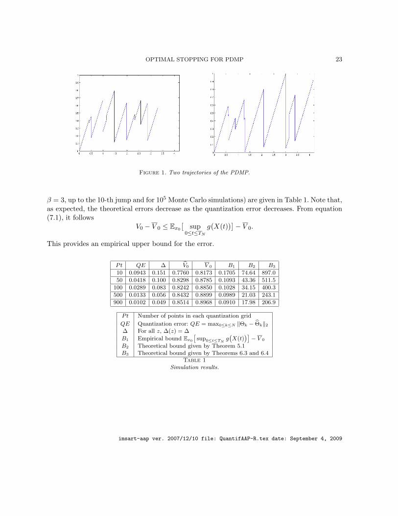
β = 3, up to the 10-th jump and for 105 Monte Carlo simulations) are given in Table 1. Note that,as expected, the theoretical errors decrease as the quantization error decreases. From equation(7.1), it follows

V0 − V 0 ≤ Ex0

[sup

0≤t≤TNg(X(t)

)]− V 0.

This provides an empirical upper bound for the error.

Pt QE ∆ V0 V 0 B1 B2 B3

10 0.0943 0.151 0.7760 0.8173 0.1705 74.64 897.0

50 0.0418 0.100 0.8298 0.8785 0.1093 43.36 511.5

100 0.0289 0.083 0.8242 0.8850 0.1028 34.15 400.3

500 0.0133 0.056 0.8432 0.8899 0.0989 21.03 243.1

900 0.0102 0.049 0.8514 0.8968 0.0910 17.98 206.9

Pt Number of points in each quantization grid

QE Quantization error: QE = max0≤k≤N ‖Θk − Θk‖2∆ For all z, ∆(z) = ∆

B1 Empirical bound Ex0

[sup0≤t≤TN

g(X(t)

)]− V 0

B2 Theoretical bound given by Theorem 5.1B3 Theoretical bound given by Theorems 6.3 and 6.4

Table 1Simulation results.



APPENDIX A: AUXILIARY RESULTS

A.1. Lipschitz properties of J and K. In this section, we derive useful Lipschitz-typeproperties of operators J and K. The first result is straightforward.

Lemma A.1 Let h ∈ Lc. Then for all (x, y) ∈ E2 and (t, u) ∈ R2+, one has∣∣∣h(φ(x, t ∧ t∗(x))

)e−Λ(x,t∧t∗(x)) − h

(φ(y, u ∧ t∗(y))

)e−Λ(y,u∧t∗(y))

∣∣∣≤ D1(h)|x− y|+D2(h)|t− u|,

where

• if t < t∗(x) and u < t∗(y),

D1(h) =[h]1

+ ChCt∗[λ]1, D2(h) =

[h]2

+ ChCλ,

• if t = t∗(x) and u = t∗(y),

D1(h) =[h]∗ + ChCt∗

[λ]1

+ ChCλ[t∗], D2(h) = 0,

• otherwise,

D1(h) =[h]1

+ ChCt∗[λ]1

+[h]2

[t∗]

+ ChCλ[t∗], D2(h) =

[h]2

+ ChCλ.

Lemma A.2 Let w ∈ B(E). Then for all x ∈ E, (t, u) ∈ R2+, one has∣∣∣J(w, g)(x, t)− J(w, g)(x, u)

)∣∣∣ ≤ (CwCλ +[g]2

+ CgCλ)|t− u|,

Proof: By definition of J , we obtain∣∣∣J(w, g)(x,t)− J(w, g)(x, u))∣∣∣ ≤ ∣∣∣∣∣

∫ u∧t∗(x)

t∧t∗(x)λQw(φ(x, s))e−Λ(x,s)ds

∣∣∣∣∣+∣∣∣g(φ(x, t ∧ t∗(x)))e−Λ(x,t∧t∗(x)) − g(φ(x, u ∧ t∗(x)))e−Λ(x,u∧t∗(x))

∣∣∣.Applying Lemma A.1 to h = g, the result follows. 2

Lemma A.3 Let w ∈ Lc. Then for all (x, y) ∈ E2, t ∈ R+,∣∣∣J(w, g)(x, t)− J(w, g)(y, t))∣∣∣ ≤ (CwE1 +

[w]1E2 + E3

)|x− y|,

where

E1 = Cλ[t∗]

+ Ct∗[λ]1

(1 + Ct∗Cλ

),

E2 = Ct∗Cλ[Q],

E3 =[g]1

+[g]2

[t∗]

+ CgCt∗[λ]1

+ Cλ[t∗]



Proof: again by definition, we obtain∣∣∣J(w, g)(x, t)− J(w, g)(y, t))∣∣∣

≤∣∣∣∣∣∫ t∧t∗(x)

0λQw(φ(x, s))e−Λ(x,s)ds−

∫ t∧t∗(y)

0λQw(φ(y, s))e−Λ(y,s)ds

∣∣∣∣∣+∣∣∣g(φ(x, t ∧ t∗(x)))e−Λ(x,t∧t∗(x)) − g(φ(y, t ∧ t∗(y)))e−Λ(y,t∧t∗(y))

∣∣∣.Without loss of generality it can be assumed that t∗(x) ≤ t∗(y). From Lemma A.1 for h = g andusing the fact that

∣∣t ∧ t∗(x)− t ∧ t∗(y)∣∣ ≤ ∣∣t∗(x)− t∗(y)

∣∣, we get∣∣∣J(w, g)(x, t)− J(w, g)(y, t))∣∣∣

≤∫ t∧t∗(x)

0

∣∣∣λQw(φ(x, s))e−Λ(x,s) − λQw(φ(y, s))e−Λ(y,s)∣∣∣ds

+(CwCλ

[t∗]

+ E3)|x− y|.

By using a similar results as Lemma A.1 for h = λQw, we obtain the result. 2

Lemma A.4 Let w ∈ Lc. Then for all (x, y) ∈ E2,∣∣Kw(x)−Kw(y)∣∣ ≤ (CwE4 +

[w]1E2 +

[w]∗[Q])|x− y|,

where E4 = 2Cλ[t∗]

+ Ct∗[λ]1

(2 + Ct∗Cλ

).

Proof: The proof is similar to the previous ones and therefore omitted. 2

A.2. Lipschitz properties of the value functions. Now we turn to the Lipschitz con-tinuity of the sequence of value functions (vn). Namely, we prove that under our assumptions,vn belongs to Lc for all 0 ≤ n ≤ N . We also compute the Lipschitz constant of vn on E as it ismuch sharper in this case than

[vn]1, see Remark 2.2.

We start with proving sharper results on operator J .

Lemma A.5 Let w ∈ Lc. Then for all x ∈ E and (s, t) ∈ R2+,∣∣∣ sup

u≥tJ(w, g)(x, u)− sup

u≥sJ(w, g)(x, u)

∣∣∣ ≤ (CwCλ +[g]2

+ CgCλ)|t− s|,

Proof: Without loss of generality it can be assumed that t ≤ s. Therefore, one has∣∣∣ supu≥t

J(w, g)(x, u)− supu≥s

J(w, g)(x, u)∣∣∣ = sup

u≥tJ(w, g)(x, u)− sup

u≥sJ(w, g)(x, u).(A.1)



Remark that there exists t ∈ [t ∧ t∗(x), t∗(x)] such that supu≥t

J(w, g)(x, u) = J(w, g)(x, t). Conse-

quently, if t ≥ s then one has∣∣∣ supu≥t


J(w, g)(x, u)∣∣∣ = 0.

Now if t ∈ [t ∧ t∗(x), s[, then one has

supu≥t


J(w, g)(x, u) ≤ J(w, g)(x, t)− J(w, g)(x, s).

From Lemma A.2, we obtain the following inequality

supu≥t


J(w, g)(x, u) ≤(CwCλ +

[g]2

+ CgCλ)|t− s|.(A.2)

Combining equations (A.1), (A.2) and the fact that |t− s| ≤ |t− s| the result follows. 2

similarly, we obtain the following result.

Lemma A.6 Let w ∈ Lc. Then for all (x, y) ∈ E2,∣∣∣ supt≤t∗(x)

J(w, g)(x, t)− supt≤t∗(y)

J(w, g)(y, t)∣∣∣ ≤ (CwE5 +

[w]1E2 + E6

)|x− y|,

where E5 = E1 + Cλ[t∗]

and E6 = E3 +([g]2

+ CgCλ)[t∗].

Now we turn to (vn). Recall from [11] that for all 0 ≤ n ≤ N , (vn) is bounded with Cvn = Cg.

Proposition A.7 For all 0 ≤ n ≤ N , vn ∈ Lc and[vn]1≤ eCλCt∗

(2[vn+1

]1E2 + CgE1 + CgE4 + CgCt∗

[λ]1(1 + CλCt∗)

)+eCλCt∗

([g]1

+[g]2

[t∗])∨([vn+1

]∗[Q])

,(A.3) [vn]2≤ eCλCt∗

CgCλ

(4 + CλCt∗

)+[g]2

,(A.4) [

vn]∗ ≤

[vn]1

+[vn]2

[t∗],[

vn]≤

[vn+1

]1E2 + CgE5 +

E6 ∨

([vn+1

]∗[Q]

+ CgCt∗[λ]1

).

Proof: Clearly, vN = g is in Lc. Assume that vn+1 is in Lc, then by using the semi-groupproperty of the drift φ it can be shown that for any x ∈ E, t ∈ [0, t∗(x)], one has (see [11, Eq.(8)])

vn(φ(x, t)) = eΛ(x,t)(

supu≥t

J(vn+1, g)(x, u) ∨Kvn+1(x))− Ivn+1(x, t)

.(A.5)

Remark that for x ∈ E, t ∈ R+, one has

supu≥t

J(vn+1, g)(x, u) ∨Kvn+1(x) ≤ supuJ(vn+1, g)(x, u) ∨Kvn+1(x) = vn(x).(A.6)



Set (x, y) ∈ E2 and t ∈ [0, t∗(x) ∧ t∗(y)]. It is easy to show that∣∣∣eΛ(x,t) − eΛ(y,t)∣∣∣ ≤ eCλCt∗

[λ]1Ct∗ |x− y|,(A.7) ∣∣∣Ivn+1(x, t)− Ivn+1(y, t)

∣∣∣ ≤ (Cvn+1E1 +

[vn+1

]1E2

)|x− y|.(A.8)

Then, equations (A.5)-(A.8) yield∣∣∣vn(φ(x, t))− vn(φ(y, t))∣∣∣ ≤ ∣∣vn(x)

∣∣+ ∣∣Ivn+1(x, t)∣∣eCλCt∗ [λ]

1Ct∗ |x− y|

+ eΛ(y,t)

supu≥t

∣∣∣J(vn+1, g)(x, u)− J(vn+1, g)(y, u)∣∣∣ ∨ ∣∣Kvn+1(x)−Kvn+1(y)

∣∣+ eΛ(y,t)

(Cvn+1E1 +

[vn+1

]1E2

)|x− y|.(A.9)

For x ∈ E, t ∈ [0, t∗(x)] and n ∈ N, note that

eΛ(x,t) ≤ eCλCt∗ ,∣∣Ivn+1(x, t)

∣∣ ≤ CλCvn+1Ct∗ , and |vn+1(x)| ≤ Cg.(A.10)

Therefore, we obtain inequality (A.3) by using equations (A.9), (A.10) and Lemma A.3, A.5,and the fact that CgE1 + E3 = CgE4 +

[g]1

+[g]2

[t∗].

Now, set x ∈ E and t, s ∈ [0, t∗(x)]. Similarly, one has∣∣∣eΛ(x,t) − eΛ(x,s)∣∣∣ ≤ eCλCt∗Cλ|t− s|,(A.11) ∣∣∣Ivn+1(x, t)− Ivn+1(x, s)∣∣∣ ≤ CλCvn+1 |t− s|.(A.12)

Combining equations (A.5), (A.6), (A.11) and (A.12), it yields∣∣∣vn(φ(x, t))− vn(φ(x, s))∣∣∣ ≤ ∣∣vn(x)

∣∣+ ∣∣Ivn+1(x, t)∣∣eCλCt∗Cλ|t− s|

+ eΛ(x,t)∣∣∣ sup

u≥tJ(vn+1, g)(x, u)− sup

u≥sJ(vn+1, g)(x, u)

∣∣∣+ CλCvn+1 |t− s|.(A.13)

Finally, inequality (A.4) follows from equations (A.10), (A.13) and Lemma A.4.

One clearly has[vn]∗ ≤

[vn]1

+[vn]2

[t∗]. Finally, set (x, y) ∈ E2. By definition, one has∣∣vn(x)− vn(y)

∣∣≤

∣∣∣ supu≤t∗(x)

J(vn+1, g)(x, u)− supu≤t∗(y)

J(vn+1, g)(y, u)∣∣∣ ∨ ∣∣Kvn+1(x)−Kvn+1(y)

∣∣,and we conclude using Lemmas A.6 and A.4, and the fact that E4 = E5 + Ct∗

[λ]1. 2

Remark A.8 Note that[vn]

is much sharper than[vn]1. If in addition to our assumptions, the

drift φ is Lipschitz-continuous in both variables, then with obvious notation, one has[vn]i≤[

vn][φ]i

for i ∈ 1, 2, ∗, which should yields better constant, see the example in Section 7.



APPENDIX B: STRUCTURE OF THE STOPPING TIMES OF PDMP’S

Let τ be anFtt∈R+

-stopping time. Let us recall the important result from M.H.A. Davis[6]

Theorem B.1 There exists a sequence of nonnegative random variables(Rn)n∈N∗ such that Rn

is FTn−1-measurable and τ ∧ Tn+1 =(Tn +Rn+1

)∧ Tn+1 on τ ≥ Tn.

Lemma B.2 Define R1 = R1, and Rk = Rk1Sk−1≤Rk−1. Then one has

τ =∞∑n=1

Rn ∧ Sn.

Proof : Clearly, on Tk ≤ τ < Tk+1, one has Rj ≥ Sj and Rk+1 < Sk+1 for all j ≤ k.Consequently, by definition Rj = Rj for all j ≤ k + 1, whence

∞∑n=1

Rn ∧ Sn =k∑

n=1

Rn ∧ Sn +Rk+1 ∧ Sk+1

+

∞∑n=k+2

Rn ∧ Sn

= Tk +Rk+1 +∞∑

n=k+2

Rn ∧ Sn.

Since Rk+1 = Rk+1 < Sk+1 we have Rj = 0 for all j ≥ k + 2. Therefore,∑∞n=1Rn ∧ Sn =

Tk +Rk+1 = τ , showing the result. 2

There exists a sequence of measurable mappings(rk)k∈N∗ defined on E × (R+ × E)k−1 with

value in R+ satisfying

R1 = r1(Z0),Rk = rk(Z0,Γk−1),

where Γk =(S1, Z1, . . . , Sk, Zk

).

Definition B.3 Consider p ∈ N∗. Let(Rk)k∈N∗ be a sequence of mappings defined on E×(R+×

E)p × Ω with value in R+ defined by

R1(y, γ, ω) = rp+1(y, γ),

and for k ≥ 2

Rk(y, γ, ω) = rp+k(y, γ,Γk−1(ω))1Sk−1≤Rk−1(y, γ, ω).



Proposition B.4 Assume that Tp ≤ τ ≤ TN . Then, one has

τ = Tp + τ(Z0,Γp, θTp),

where τ : E × (R+ × E)p × Ω→ R+ is defined by

τ(y, γ, ω) =N−p∑n=1

Rn(y, γ, ω) ∧ Sn(ω).(B.1)

Proof : First, let us prove by induction that for k ∈ N∗, one has

Rk(Z0,Γp, θTp) = Rp+k.(B.2)

Indeed, one has R1(Z0,Γp, θTp) = Rp+1, and on the set τ ≥ Tp, one also has Rp+1 = Rp+1.Consequently, R1(Z0,Γp) = Rp+1. Now assume that Rk(Z0,Γp, θTp) = Rp+k. Then, one has

Rk+1(Z0(ω),Γp(ω), θTp(ω)) = rp+k+1(Z0(ω),Γp(ω),Γk(θTp(ω)))1Sk≤Rk(Z0(ω),Γp(ω), θTp(ω)).

By definition, one has Γk(θTp(ω)) =(Sp+1(ω), Zp+1(ω), . . . , Sp+k(ω), Zp+k(ω)

)and the induction

hypothesis easily yields 1Sk≤Rk(Z0(ω),Γp(ω), θTp(ω)) = 1Sp+k≤Rp+k(ω). Therefore, we get

Rk+1(Z0,Γp, θTp) = Rp+k+1, showing (B.2).

Combining equations (B.1) and (B.2) yields

τ(Z0,Γp, θTp) =N−n∑n=1

Rp+n ∧ Sp+n.(B.3)

However, we have already seen that on the set T ≥ Tp, one has Rk = Rk ≥ Sk, for k ≤ p.Consequently, using equation (B.3), we obtain

Tp + τ(Z0,Γp, θTp) =p∑

k=1

Sk +N∑

k=p+1

Rk ∧ Sk =N∑k=1

Rk ∧ Sk.

Since τ ≤ TN , we obtain from Lemma B.2 and its proof that τ =N∑n=1

Rn ∧ Sn, showing the

result. 2

Proposition B.5 Let(Un)n∈N∗ be a sequence of nonnegative random variables such that Un is

FTn−1-measurable and Un+1 = 0 on Sn > Un, for all n ∈ N∗. Set

U =∞∑n=1

Un ∧ Sn.

Then U is anFtt∈R+

-stopping time.



Proof : Assumption 2.1 yields

U ≤ t =∞⋃n=0

[(Tn ≤ U < Tn+1∩U ≤ t∩t < Tn+1

)∪(Tn ≤ U < Tn+1∩U ≤ t∩Tn+1 ≤ t

)](B.4)

From the definition of Un, one has U ≥ Tn = Un ≥ Sn, hence one has

Tn ≤ U < Tn+1∩U ≤ t∩t < Tn+1 =Sn ≤ Un∩Tn + Un+1 ≤ t∩Tn ≤ t∩t < Tn+1

Theorem 2.10 ii) in [8] now yields Sn ≤ Un∩Tn + Un+1 ≤ t∩Tn ≤ t ∈ Ft, thus one has

Tn ≤ U < Tn+1∩U ≤ t∩t < Tn+1 ∈ Ft.(B.5)

On the other hand, one has

Tn ≤ U < Tn+1∩U ≤ t∩Tn+1 ≤ t = Sn ≤ Un∩Un+1 < Sn+1∩Tn+1 ≤ t

Hence Theorem 2.10 ii) in [8] again yields

Tn ≤ U < Tn+1∩U ≤ t∩Tn+1 ≤ t ∈ Ft.(B.6)

Combining equations (B.4), (B.5), and (B.6) we obtain the result. 2

Corollary B.6 For any (y, γ) ∈ E×(R+×E

)p, τ(y, γ, .) is anFtt∈R+

-stopping time satisfyingτ(y, γ, .) ≤ TN−p.

Proof : It follows form the definition of Rk that Rk(y, γ, ω) < Sk(ω) implies Rk+1(y, γ, ω) = 0and the nonnegative random variable Rk(y, γ, .) is FTk−1

-measurable. Therefore, Proposition B.5yields that τ(y, γ, .) is an

Ftt∈R+

-stopping time. finally, by definition of τ , see equation (B.1),

one has τ(y, γ, .) ≤N−p∑n=1

Sn = TN−p showing the result. 2

REFERENCES

[1] Bally, V., and Pages, G. A quantization algorithm for solving multi-dimensional discrete-time optimalstopping problems. Bernoulli 9, 6 (2003), 1003–1049.

[2] Bally, V., Pages, G., and Printems, J. A quantization tree method for pricing and hedging multidimen-sional American options. Math. Finance 15, 1 (2005), 119–168.

[3] Costa, O. L. V., and Davis, M. H. A. Approximations for optimal stopping of a piecewise-deterministicprocess. Math. Control Signals Systems 1, 2 (1988), 123–146.

[4] Costa, O. L. V., and Dufour, F. Stability and ergodicity of piecewise deterministic Markov processes.SIAM J. Control Optim. 47, 2 (2008), 1053–1077.



[5] Costa, O. L. V., Raymundo, C. A. B., and Dufour, F. Optimal stopping with continuous control ofpiecewise deterministic Markov processes. Stochastics Stochastics Rep. 70, 1-2 (2000), 41–73.

[6] Davis, M. H. A. Markov models and optimization, vol. 49 of Monographs on Statistics and Applied Proba-bility. Chapman & Hall, London, 1993.

[7] Dufour, F., and Costa, O. L. V. Stability of piecewise-deterministic Markov processes. SIAM J. ControlOptim. 37, 5 (1999), 1483–1502 (electronic).

[8] Elliott, R. J. Stochastic calculus and applications, vol. 18 of Applications of Mathematics (New York).Springer-Verlag, New York, 1982.

[9] G‘atarek, D. On first-order quasi-variational inequalities with integral terms. Appl. Math. Optim. 24, 1

(1991), 85–98.

[10] Gray, R. M., and Neuhoff, D. L. Quantization. IEEE Trans. Inform. Theory 44, 6 (1998), 2325–2383.Information theory: 1948–1998.

[11] Gugerli, U. S. Optimal stopping of a piecewise-deterministic Markov process. Stochastics 19, 4 (1986),221–236.

[12] Kushner, H. J. Probability methods for approximations in stochastic control and for elliptic equations.Academic Press [Harcourt Brace Jovanovich Publishers], New York, 1977. Mathematics in Science andEngineering, Vol. 129.

[13] Lenhart, S., and Liao, Y. C. Integro-differential equations associated with optimal stopping time of apiecewise-deterministic process. Stochastics 15, 3 (1985), 183–207.

[14] Pages, G. A space quantization method for numerical integration. J. Comput. Appl. Math. 89, 1 (1998),1–38.

[15] Pages, G., and Pham, H. Optimal quantization methods for nonlinear filtering with discrete-time obser-vations. Bernoulli 11, 5 (2005), 893–932.

[16] Pages, G., Pham, H., and Printems, J. An optimal Markovian quantization algorithm for multi-dimensional stochastic control problems. Stoch. Dyn. 4, 4 (2004), 501–545.

[17] Pages, G., Pham, H., and Printems, J. Optimal quantization methods and applications to numericalproblems in finance. In Handbook of computational and numerical methods in finance. Birkhauser Boston,Boston, MA, 2004, pp. 253–297.

IMB, 351 cours de la Liberation, F33405 Talence, FranceE-mail: [email protected]: [email protected]: [email protected]

IMB, 351 cours de la Liberation, F33405 Talence, France


Numerical method for optimal stopping of piecewise deterministic Markov processes

Documents

Transcript of Numerical method for optimal stopping of piecewise deterministic Markov processes