Copyright 2002, Intel Corporation, All rights reserved.

A Linear Programming Formulation of Flows over Time with Piecewise Constant Capacity and Transit Times Juan Alonso and Kevin Fall IRB-TR-03-007 June, 2003

DISCLAIMER: THIS DOCUMENT IS PROVIDED TO YOU "AS IS" WITH NO WARRANTIES WHATSOEVER, INCLUDING ANY WARRANTY OF MERCHANTABILITY NON-INFRINGEMENT, OR FITNESS FOR ANY PARTICULAR PURPOSE. INTEL AND THE AUTHORS OF THIS DOCUMENT DISCLAIM ALL LIABILITY, INCLUDING LIABILITY FOR INFRINGEMENT OF ANY PROPRIETARY RIGHTS, RELATING TO USE OR IMPLEMENTATION OF INFORMATION IN THIS DOCUMENT. THE PROVISION OF THIS DOCUMENT TO YOU DOES NOT PROVIDE YOU WITH ANY LICENSE, EXPRESS OR IMPLIED, BY ESTOPPEL OR OTHERWISE, TO ANY INTELLECTUAL PROPERTY RIGHTS

A Linear Programming Formulation of Flows over Time with

piecewise constant capacity and transit times

Juan Alonso1 and Kevin Fall2

1 Swedish Institute of Computer Science, Stockholm Sweden2 Intel Research, Berkeley USA

Abstract. We present an algorithm to solve a deterministic form of a routing problem in delay tolerantnetworking, in which contact possibilities are known in advance. The algorithm starts with a finite setof contacts with time-varying capacities and transit delays. The output is an optimal schedule assigningmessages to edges and times, that respects message priority and minimizes the overall delivery delay.The algorithm consists of two main ingredients: a discretization step in which the raw data providedby the contacts is used to obtain appropriate subdivisions of the relevant time intervals, and a linearprogram, a dynamic version of the classical multicommodity flow problem, in which transit times arepiecewise constant, and where both edges and nodes are capacitated (in the case of edges, with piece-wise constant capacities). In fact, we present two equivalent LP formulations, of which one is smallerand runs faster in CPLEX, a general purpose linear solver.

1 Introduction

Route selecting in data networks typically consists of selection of shortest paths in a connecteddirected (or undirected) graph. In this work, we look at the problem of optimal message routing in adelay tolerant network (DTN)[1], which is assumed to suffer from frequent partitioning such that nocontemporaneous end-to-end path may ever exist. In graph theoretic terms, this problem is a formof dynamic multicommodity flow or quickest transshipment problem in which both edge capacitiesand transit delays along an edge can vary as a function of time and are permitted to be zero,and finite buffer capacities are assigned to each vertex. Examples of real networks exhibiting suchbehavior include Low-Earth Orbiting Satellites, which provide network connectivity for predictableintervals of time (and at predictable capacities) based on orbital mechanics.

For purposes of this study, we assume that a set of vertices V and a set of contacts are given. Acontact C is a directed edge between two vertices in V for a particular interval of time in which aconstant capacity and latency is available to carry commodity flow. More precisely, a contact C isa 4-tuple (e, I, c, d), where e ∈ V × V , I is a time interval during which flow is permitted to departalong edge e, and c, d are non-negative real numbers representing edge capacity and transit time,respectively. In practice, the time intervals are finite for contacts describing links (communicationopportunities) that come and go periodically or occasionally, and are (−∞,∞) for persistent ones(persistent links are thus assumed to have a perpetual constant capacity and delay). Given the setof vertices and contacts, we construct the routing (multi)graph G = (V,E) where E = {e|e is anedge in any contact given}.

In addition to the topology elements of vertices and contacts, we assume that each vertex alsohas an associated maximum buffer capacity bv, and that there is a commodity demand matrix Mknown in advance where M = {mk,p|k = (u, v) ∈ V × V, p ∈ (1 . . . 4)}, where p is a priority level.In addition, we assume a weight function w(p) to be given that gives the relative penalty paid fordelaying high-priority traffic. Its use is explained below.

Our approach is to use a linear programming formulation of this problem, as it is perhaps themost natural mechanism to express the various constraints. Our goal is to capture the essence of theproblem as closely as possible, with less emphasis on proof of polynomial-time algorithm operation.Future work will pursue the computational complexity of this problem, and of related problems inwhich M or E are not deterministically known with certainty in advance.

2 A system of time intervals

As mentioned above, the model requires special care with the time intervals used. In the LPformulation of the problem given in Section 3, it is assumed that we are given a system of timeintervals and subdivision points satisfying a certain property (see condition (i) below). In thissection we explain how to obtain (some of) these subdivision points from first principles (i.e. fromthe contacts described above). In Sections 4 and 5, we complete the algorithm and give proofs thatthe subdivision points so constructed do satisfy the required condition.

We assume that G is constructed as described above and that ”reality” has provided us witha finite set C = {C1, . . . , Cn} of contacts. Here ”reality” also means that when the delay (and/orcapacity) of a certain link is not constant over a given time interval, we subdivide the time intervalinto subintervals so that the variable delay can be satisfactorily approximated by constant delaysover the subintervals. This situation will thus be modelled as a finite number of contacts of thetype defined above.

By collecting the endpoints of all finite time intervals of contacts in C, we form a set T1 oftime-points, i.e.3

T1 = {t|∃C = (e, I, c, d) ∈ C with I finite, such that t = ι(I) or t = τ(I)}.

We can think of T1 as a subdivision of the transmission time interval [t0, th], where t0 = min T1, andth = max T1. Collecting the delays of all contacts, we form the set D = {d|d is the delay of some C ∈C}, and set ∆ = max D. We also have a reception interval [t0, th + ∆] and an extended interval[t0 − ∆, th + ∆], see Fig. 1. Observe that transmission on any link occurs entirely in time-interval[t0, th] and that, due to delay, transmissions are (completely) received in the period [t0, th + ∆](notice that delay can be zero in some links).

-

transmission

reception

extended

th + ∆t0 − ∆ tht0

Fig. 1. Time intervals.

We extend T1 to T2 = T1 ∪ {t0 − ∆, th + ∆}. Observe that T2 is a subdivision of the extendedinterval, T2 ∩ [t0, th + ∆] is a subdivision of the reception interval, and T1 = T2 ∩ [t0, th] is a

3 Here, for any ordered pair X = (a, b), ι(X) = a and τ (X) = b.

2

subdivision of the transmission interval. At every subdivision, T2 generates a set of subintervals(of the extended interval), denoted I2, as follows. If T2 = {t0 − ∆, t0, t1, . . . , th, th + ∆}, thenI2 = {[t0 − ∆, t0], [t0, t1], . . . , [th, th + ∆]}.

Next, we define a capacity function c : E × I2 → R+ ∪ {0} [resp. delay function d : E × I2 →R+ ∪{0}]. The set of contacts satisfy constraints that imply that, given a pair (e, I) ∈ E ×I2, onlyone of the following possibilities can occur: there is a unique contact C ′ = (e′, I ′, c′, d′) ∈ C withe = e′ and I ⊆ I ′, or else no contact involving e has a time interval containing I. In the first casewe define ce,I = c′ [resp. de,I = d′], and in the second case ce,I = 0 [resp. de,I = 0].

At this point we have constructed a time axis and identified transmission, reception and ex-tended intervals which are provided with compatible subdivisions. To proceed further and definethe required property, we need to further subdivide the constructed intervals. More exactly, weneed to refine the given subdivisions T1 and T2. The precise details of the construction and proofsare given later, in sections 4 and 5 below. For the time being, we content ourselves with makingprecise the assumptions needed for the LP formulation.

Thus, assume we are given a finite subdivision TE of the extended interval [t0 −∆, th + ∆]. Wewill assume, moreover, that TE contains t0 and th. This condition ensures that TX = TE ∩ [t0, th]and TR = TE ∩ [t0, th + ∆] are (finite) subdivisions of the transmission interval [t0, th] and of thereception interval [t0, th + ∆], respectively.

From these subdivisions we generate subintervals in the usual way: order the elements of, say,TE and let IE consist of all intervals of the form [ti, ti+1], where ti, ti+1 are consecutive elementsof TE . Observe that |IE| = |TE | − 1, the intersection of any pair of different subintervals of IE

is either a point of empty, and the union of all of them is the extended interval [t0 − ∆, th + ∆].Similarly, TX [resp. TR] defines a set of subintervals IX [resp. IR] whose union is the transmission[resp. reception] interval. Observe that IX ⊆ IR ⊆ IE.

For an interval I = [a, b] and real number d, we let I ± d denote the interval [a ± d, b ± d]. Thecondition mentioned above can be expressed as follows:

i) ∀d ∈ D ∀I ∈ IR, I − d ∈ IE

In the input to the problem formulated below we assume that this condition is satisfied.

3 LP formulation

In this section we describe a linear programming model for the routing problem described in Section1. The model is a dynamic version of the classical multicommodity flow problem. The commoditiesare source-destination pairs. Another appropriate choice of commodities would have been triplesof the form source-destination-priority. We model delay by distinguishing between transmissionand reception, i.e. we introduce two parallel sets of variables, one set to take care of transmission(transmission variables are denoted X) and the other to take care of reception (reception variablesare denoted R). In the model, we consider transmission to be the primal activity and reception thederived one. We begin by giving a list of the input to the model.

Sets and Functions

G directed graph, G = (V,E)TE finite subdivision of [t0 − ∆, th + ∆]TX finite subdivision of [t0, th] induced by TE , TX = TE ∩ [t0, th]

3

TR finite subdivision of [t0, th + ∆]

induced by TE, TR = TE ∩ [t0, th + ∆]IE set of time intervals induced by TE

IX set of time intervals induced by TX

IR set of time intervals induced by TR

c c : E × IE → R+ ∪ {0}, where ce,I is the (transmission) capacity of edge e on time intervalI ∈ IE, and ce,I = 0 for all e, whenever I ⊆ [t0 − ∆, t0] ∪ [th + ∆]

d d : E × IE → R+ ∪ {0}, where de,I is the propagation delay of edge e during time intervalI ∈ IE,

and de,I = 0 for all e, whenever I ⊆ [t0 − ∆, t0] ∪ [th + ∆]K set of commodities, K ⊆ V × VP set of priorities, P = {1, 2, 3, 4}w weight function w : P → R+,

strictly monotone decreasingIv set of incoming edges (arc heads) at node vOv set of outgoing edges (arc tails) at node v

Constants

∆ largest delay, ∆ = max Dbv buffer capacity of node vmk,` size of all messages from ι(k) to τ(k) which have priority `

Variables

Nk,`v,t amount of commodity k of priority ` occupying the buffer at node v at time t ∈ TR

Xk,`e,I amount of data from ι(k) to τ(k) and priority ` that is transmitted at ι(e) (sent to τ(e))

during I ∈ IE

Rk,`e,I amount of data from ι(k) to τ(k) and priority ` that is received at τ(e) (coming from ι(e))

during I ∈ IR

When e = (v, w) is a link from node v to node w, we let ι(e) = v denote the initial point (arc tail)

of e, and τ(e) = w denote its terminal point (arc head). Note that X k,`e,I has been defined for

I ∈ IE, i.e. even for I outside the transmission interval. This does not contradict the fact thattransmission occurs only for I ∈ IX since it will turn out (from equations (5) below, together with

the conditions on c imposed above) that Xk,`e,I = 0 for all I ⊆ [t0 − ∆, t0] ∪ [th + ∆]. Observe once

again that c stands for the capacity of an edge at its tail (the departing point of a link). It is animplicit assumption of the model that the receiver at the far end of the link is capable of receivingat the appropriate times so that all transmissions (occurring at the initial point of the link) over[t0, th] will be received (at the end point of the link) over [t0, th + ∆].In formulas (1) (2) below we need to relate time intervals to their endpoints. We do this byassuming the time intervals are numbered I1, . . . , Iq, . . . , and satisfy Iq = [tq−1, tq].

LP formulation

min∑

`∈P

∑

k∈K

∑

e∈E

∑

Iq∈IX

w(`) · tq · Xk,`e,Iq

(1)

4

subject to

∑

w∈Iv

Rk,`

(w,v),Iq−

∑

w∈Ov

Xk,`

(v,w),Iq= Nk,`

v,tq− Nk,`

v,tq−1, k, `, v, Iq ∈ IR (2)

Rk,`e,I = Xk,`

e,(I− de,I ), k, `, e, I ∈ IE (3)∑

`∈P

∑

k∈K

Nk,`v,t ≤ bv, k, `, v, t ∈ TR (4)

∑

`∈P

∑

k∈K

Xk,`e,I ≤ ce,I · |I|, k, `, e, I ∈ IE (5)

∑

I∈IR

∑

w∈Ov

Xk,`

(v,w),I −∑

I∈IR

∑

w∈Iv

Rk,`

(w,v),I

0 if v 6= ι(k) & v 6= τ(k)

mk,` if v = ι(k)

−mk,` if v = τ(k)

(6)

Nk,`v,t0

=

mk,` if v = ι(k)

0 if v 6= ι(k), k, `, v (7)

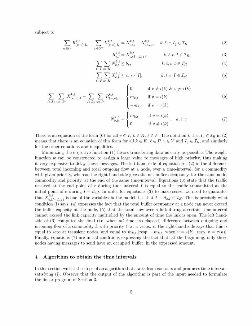
There is an equation of the form (6) for all v ∈ V, k ∈ K, ` ∈ P . The notation k, `, v, Iq ∈ IR in (2)means that there is an equation of this form for all k ∈ K, ` ∈ P, v ∈ V and Iq ∈ IR, and similarlyfor the other equations and inequalities.

Minimizing the objective function (1) favors transferring data as early as possible. The weightfunction w can be constructed to assign a large value to messages of high priority, thus makingit very expensive to delay these messages. The left-hand side of equation set (2) is the differencebetween total incoming and total outgoing flow at a node, over a time-interval, for a commoditywith given priority, whereas the right-hand side gives the net buffer occupancy, for the same node,commodity and priority, at the end of the same time-interval. Equations (3) state that the trafficreceived at the end point of e during time interval I is equal to the traffic transmitted at theinitial point of e during I − de,I . In order for equations (3) to make sense, we need to guarantee

that Xk,`

e,(I−de,I ) is one of the variables in the model, i.e. that I − de,I ∈ IE. This is precisely what

condition (i) says. (4) expresses the fact that the total buffer occupancy at a node can never exceedthe buffer capacity at the node, (5) that the total flow over a link during a certain time-intervalcannot exceed the link capacity multiplied by the amount of time the link is open. The left hand-side of (6) computes the final (i.e. when all time has elapsed) difference between outgoing andincoming flow of a commodity k with priority `, at a vertex v; the right-hand side says that this isequal to zero at transient nodes, and equal to mk,` [resp. −mk,`] when v = ι(k) [resp. v = τ(k)].Finally, equations (7) are initial conditions expressing the fact that, at the beginning, only thosenodes having messages to send have an occupied buffer, in the expressed amount.

4 Algorithm to obtain the time intervals

In this section we list the steps of an algorithm that starts from contacts and produces time intervalssatisfying (i). Observe that the output of the algorithm is part of the input needed to formulatethe linear program of Section 3.

5

0) Start with a set of contacts and vertices, and construct the directed graph G = (V, E).

1) Extract the time points to form T1 and the delays to form D. Set ∆ = max D.

2) Set t0 = min T1, th = max T1. Set T2 = T1 ∪ {t0 − ∆, th + ∆}.

3) From T2 construct the induced set I2 of subintervals.

4) Use the contacts to define the capacity and delay functions c, d : E × I2 → R + ∪{0}.

5) Form the set D′ = D ∪ {|ti − ti−1| : ti−1, ti are consecutive elements of T2} and denote its elements

D′ = {d1, . . . , dN}.

6) Approximate the numbers in D′ by rational numbers. From now on, we assume the elements of D ′

have the form di = ni/mi, for appropriate integers ni, mi.

7) Compute q = lcm{m1, . . . , mN}, p = gcd{n1 · (q/m1), . . . , nN · (q/mN )}, and set ε = p/q.

8) Let Tε = {t0 + ` · ε|` ∈ Z}. Then the subdivisions TE = Tε ∩ [t0 − ∆, th + ∆], TR = Tε ∩ [t0, th + ∆], and

TX = Tε ∩ [t0, th] of, respectively, the extended, reception and transmission intervals, together

with their induced set of subintervals IE , IR, and IE satisfy condition (i).

9) Use 4) to define capacity and delay functions c, d : E × IE → R + ∪{0}.

Steps 0)-4) were explained in section 2. Steps 5)-8) are discussed in the next section. For step9), use the fact that every interval in IE is contained in a unique interval in I2, together with thefunctions defined in step 4), to extend these definitions to E × IE.

5 Proofs

The basic idea behind steps 5)-8) is to subdivide the set of time points so that the correspondingtime intervals have the property that, when translated by a delay (i.e. going from I to I + de,I),they remain time intervals. In this section we give a recipe to do this, show that it is efficient, andprove that the resulting time intervals have the stated property. The crucial step to achieve thisis the construction of ε, a positive rational number with the property that every delay and everylength of an interval in I2 is an integral multiple of ε (cfr. Corollary 1 below).

Suppose we are given sets T = {t0, . . . , th} and D = {d} as above. Note that T = T1 of theprevious sections; we use T here to simplify the notation. We enlarge D by adding the lengths ofthe subintervals defined by T1, thus D′ = D ∪ {t1 − t0, . . . , th − th−1}. We assume the elements ofD′ to be rational numbers, say D′ = {d1, . . . , dN} with di = ni/mi (ni,mi ∈ Z). Furthermore, weassume that the fractions cannot be simplified and that 0, if it is an element of D ′, is representedas 0/1. Let

q = lcm(m1, . . . ,mN ), p = gcd(n1 · (q/m1), . . . , nN · (q/mN ))

and set ε = pq. Note that ε is a positive rational number. The main property of this number is

that any integral linear combination of the di is an integral multiple of ε. This can be expressedmore formally as follows. Let Zd = {` · d|` ∈ Z} denote the set of integral multiples of d, and letA + B = {a + b|a ∈ A, b ∈ B} denote the set of sums of elements of A and B. With this notationwe have:

Lemma 1.

Zd1 + · · · + ZdN = Zε

Proof. Note that p is defined as the greatest common divisor of a finite number of integers. Bywell-known properties of the gcd, it follows that

Z(n1 · (q/m1)) + · · · + Z(nN · (q/mN )) = Zp (8)

6

To prove Zε ⊆ Zd1 + · · · + ZdN it suffices to show that ε can be expressed as an integral linearcombination of the di. By (8),

p = `1 · n1 · (q/m1) + · · · + `N · nN · (q/mN )

for appropriate integers `1, . . . , `N . Dividing by q,

ε = p/q = `1 · d1 + · · · + `N · dN

as desired. The reversed inclusion is proved similarly. This concludes the proof.

Corollary 1. ε divides every di ∈ D′, i.e. di/ε ∈ Z.

Proof. Since di = 0 · d1 + · · · + 1 · di + · · · + 0 · dN is an integral linear combination of the elementsof D′, Lemma 1 implies di = r · ε for some integer r, as desired.

Given T and ε as above, let Tε = {t0 + ` · ε|` ∈ Z}. Note that, despite the notation, Tε is actuallydefined by both T and D.

Lemma 2. T is contained in Tε, i.e. T ⊆ Tε.

Proof. The lemma follows easily from Corollary 1. For instance, since we can find an integer r suchthat t1 − t0 = r · ε, it follows that t1 = t0 + r · ε is in Tε. The proof can be completed by induction.

In the next result we use the notation A ± b = {a ± b|a ∈ A}.

Lemma 3. For all d ∈ D′, Tε ± d = Tε.

Proof. We show that Tε ⊆ Tε + d. By Corollary 1, there is an integer r such that d = r · ε. Thent0 + ` · ε = t0 + (` − r) · ε + d ∈ Tε + d, since (` − r) is an integer. The reversed inclusion is provedsimilarly. Similarly for − instead of +.

Lemma 4. Suppose that Y ⊆ R is a subset of realnumbers that satisfies:

i) T ⊆ Yii) for all d ∈ D′, Y + d = Y

then Tε ⊆ Y .

Proof. Observe that condition Y + d = Y is equivalent to Y − d = Y . Next, for any A ⊆ R weconstruct inductively a set D(A) as follows. Set D0(A) = A, D1(A) = {a ± d|a ∈ A, d ∈ D′},Dn(A) = D1(Dn−1(A)) for n ≥ 2, and define

D(A) =⋃

n≥0

Dn(A).

Note that if A ⊆ Y , then D1(A) ⊆ Y (by (ii) and the observation at the beginning of the proof).This, together with the fact that both D0(T ) and D1(T ) are subsets of Y , imply that D(T ) ⊆ Y .

We complete the proof by showing that Tε ⊆ D(T ). Suppose that ε = `′1 · d1 + · · · + `′N · dN , byLemma 1. Then a typical element of Tε has the form t0 + r · ε = t0 + `1 · d1 + · · · + `N · dN , where`i = r · `′i. But t0 + `1 · d1 ∈ D`1(T ), (t0 + `1 · d1) + `2 · d2 ∈ D`2(D`1(T )) = D`1+`2(T ), and so on.We conclude that t0 + r · ε ∈ D`1+···+`N (T ) ⊆ D(T ), as desired (a similar argument shows that Tε

is actually equal to D(T ), but we don’t need this fact). This concludes the proof.

7

Theorem 1 below shows that the constructed set Tε is efficient, in the sense that it is contained inany other set satisfying similar conditions.

Theorem 1. Tε is the smallest set of numbers that contains T and is closed under translation byelements of D′.

Proof. Let Y denote the smallest set that contains T and is closed under translation by D ′. ByLemma 4, Tε ⊆ Y . By Lemma 2 and 3, Tε contains T and is closed under translation by D ′. SinceY is the smallest such set, Y ⊆ Tε, as desired.

Next, let TE = Tε ∩ [t0 −∆, th + ∆], TR = Tε ∩ [t0, th + ∆], and TX = Tε ∩ [t0, th], together withtheir induced set of subintervals IE, IR, and IE be as in 9) of the previous section. We will showthat condition (i) is satisfied.

Theorem 2. Condition (i) of section 2 is satisfied, i.e. for all d ∈ D and I ∈ IR, we haveI − d ∈ IE.

Proof. Consider an interval of the form

Ir = [t0 + r · ε, t0 + (r + 1) · ε]

for some integer r. Lemma 3 implies that, for all d ∈ D ′, Ir ± d = Is for some integer s. In otherwords, translation by elements of D ′ permutes the set of intervals of the form Ir. To complete theproof of (i) it remains only to check that if Ir is in IR (i.e. if Ir ⊆ [t0, th + ∆]), then Ir − d ∈ IE

(i.e. Ir − d ⊆ [t0 − ∆, th + ∆]). This is trivially true.

6 An equivalent LP formulation

In this section we present an equivalent formulation of the program in Section 3. A possible ad-vantage of the new formulation is that the program itself, even though the number of constraintsis unchanged, becomes smaller because the new constraints can be expressed more succinctly. Wehave tried the two formulations on CPLEX 7.1 (with default settings). The text file for the tighterformulation is, in our example, about 20% smaller and runs about 10% faster than the formulationin section 3.

To derive the new formulation, notice that, up to sign, the left-hand side of each equation oftype (6), denoted LHS(6), equals the sum over I ∈ IR of the left-hand side of the correspondingequation of type (2), denote LHS(2). On the other hand, the sum over I ∈ IR of the right-handside of an equation of type (2), denoted RHS(2) is a ”telescopic” sum that simplifies, collapsingto the difference of the last and initial terms. In symbols (where, in order to simplify the notation,we let tf = th + ∆ denote the last time point, and tf−1 denote the previous one),

−LHS(6) =∑

I∈IR

LHS(2)∑

I∈IR

(Nk,`v,tq

− Nk,`v,tq−1

) (9)

= Nk,`v,t1

− Nk,`v,t0

+ Nk,`v,t2

− Nk,`v,t1

+ · · · + Nk,`v,tf

− Nk,`v,tf−1

(10)

= Nk,`v,tf

− Nk,`v,t0

= −RHS(6) (11)

8

Finally, from equations (7) and (11) we obtain:

Nk,`v,tf

=

mk,` if v = τ(k)

0 if v 6= τ(k)(12)

We have thus shown that the ”old” polyhedron, defined by the constraints (2)-(7), is containedin the polyhedron defined by the constraints (2)-(5) together with the constraints (7) and (12).However,it is easy to see that the converse is also true: the two polyhedra coincide. Thus, the newprogram: minimize the objective function (1) subject to equations (2), (3), (4), (5), (12) and (7),is equivalent to the program in section 3.

The interpretation of the set of equations (12) is clear: it requires that, at the final time, onlythe node τ(k) will contain commodity k (of any priority) in the amount mk,`, while all other nodeswill be empty of this commodity (any priority).

7 Related Work

The formulation of max flow for networks with constant positive capacities and arc traversal timesoriginates with Ford and Fulkerson[4, 5], where a time-expanded graph is used to capture both arccapacities as well as transit delays. Variations and extensions of this approach have been used exten-sively in approaches to several flows-over-time problems including maximum flow, transshipment,and others. The attraction of time-expanded graphs arises due to the ability to take advantageof the rich set of algorithms for static graphs that can be applied to the time expanded graph tosolve flows-over-time problems. The primary disadvantage of these approaches relates to the non-polynomial growth in graph size when constructing the time-expanded graph, which is generallyexpanded as a function of the time discretization selected. By using coarser discretizations, efficientapproximation algorithms have been developed. Fleischer and Skutella construct a condensed timeexpanded graph[7] which can improve the time-expanded graph size down to a polynomial of theoriginal graph and can potentially be used as the basis for approximating the solutions of severalother flows over time problems.

When multiple sources and sinks are considered for the flows-over-time problem, a straightfor-ward time expanded graph construction is not sufficient. Hoppe and Tardos[6] study the quickesttransshipment problem, discovering it to be much more challenging than the case with a singlesource/sink pair. The overall “complexity landscape” of these problems is described in a nice re-view by Kohler, Mohring, and Skutella[2]. In[8], reference is made to a personal communication byA. Hall and M. Skutella indicating the multicommodity flows over time problem is NP-hard.

Note that virtually all of the approaches above rely on construction of a form of time-expandedgraph generated from the original graph. In our work, we instead formulate the problem directlywith respect to the given graph as a linear program. As a consequence, however, we must constructa special time interval set that is in some ways analogous to the arcs in a time-expanded graph.

For completeness, it is worth mentioning that several researchers have begun to focus on prob-lems involving flows over time in graphs where arc traversal times are a function of the flowsassigned to the arc. Such cases arise in the modelling of congested networks, including highways.These problems can be daunting, given the highly complex arc delay functions thought to exist for

9

real-world traffic network situations. This problem is more complicated than the one we are explor-ing here for a variety of reasons, and the interested reader is referred to Carey and Subrahmanian[9]and Kohler, Langkau and Skutella[3].

8 Conclusions

We have presented and algorithm to solve a version of a routing problem in delay tolerant networkingin which contact possibilities are known in advance. The algorithm starts with a finite set of contactswith (possibly variable) capacities and delays, and produces an optimal schedule assigning messagesto edges and times, that respects message priority and minimizes the overall delivery delay.

There are two steps to the algorithm. A first crucial step is to obtain from the contacts adiscretization of time satisfying a certain property (Sections 2, 4 and 5). In the usual treatment ofdynamic flow problems in the literature, discrete time plays the role of a ”period” or ”phase” tobe repeated. By contrast, in delay tolerant networking the time points at which to inject flow, aswell as for how long, are of the utmost importance.

The second step is to formulate a linear program that captures the characteristics of the prob-lem. In fact, we present two equivalent LP formulations of the problem, of which one is smaller andruns faster in CPLEX, a general purpose linear solver. The linear programs are dynamic versionsof the classical multicommodity flow problem, where both edges and nodes are capacitated (in thecase of edges, with piece-wise constant capacities). Delay is modelled by distinguishing betweentransmission and reception: a set of variables is introduced to deal with transmission (at the be-ginning of a link) and another set to deal with reception (at the endpoint of the link). Variablesin the two sets are related by the condition that whatever was transmitted (at the beginning of alink) during a certain time interval, is received (at the end of the link) during the same intervaltranslated by the delay the link in question has during the given time interval.

References

[1] K. Fall “A Delay Tolerant Network Architecture for Challenged Internets” Proc. SIGCOMM 2003 Aug., 2003[2] E. Kohler, R. Mohring, M. Skutella. “Traffic Networks and Flows over Time” TU-Berlin Technical Report

752/2002 2002.[3] E. Kohler, K. Langkau, M. Skutella. “Time-Expanded Graphs for Flow-Dependent Transit Times” TU-Berlin

Technical Report 751/2002 2002.[4] L.R. Ford, D.R. Fulkerson Flows in Networks Princeton University Press Princeton, NJ, 1962[5] L.R. Ford, D.R. Fulkerson “Constructing maximal dynamic flows from static flows” Operations Research

6:419-433, 1958[6] B. Hoppe, E. Tardos “The quickest transshipment problem” Proc. 6th ACM-SIAM symp. on Discrete Algorithms

(SODA) 1995[7] L. Fleischer, M. Skutella “The quickest multicommodity flow problem” in Integer Programming and Combi-

natorial Optimization W.J. Cook, A.S. Schulz, eds Lecture Notes in Computer Science, vol 2337 2002, pp.36-53

[8] L. Fleischer, M. Skutella “Minimum Cost Flows over Time without Intermediate Storage” Proc. SODA 2003[9] M. Carey, E. Subrahmanian “An approach to modelling time-varying flows on congested networks” Trans-

portation Research B Volume 34 (2000), pp.157-183

10