Global dynamics in a non-linear model of the equity ratio

Anna Agliari a, Laura Gardini a,b,*, Domenico Delli Gatti c, Mauro Gallegati d

a University di Parma, Faculty of Economics, Viale Kennedy, Italyb Instituto di Scienze Economiche, University di Parma and University of Urbino, 61029 Urbino, Italy

c Catholic University in Milan, Italyd University of Teramo, Italy

Accepted 5 October 1998

Abstract

A model for ®rms' ®nancial conditions is proposed, which ultimately reduces to a two-dimensional non-invertible map in the

variables mean and variance of the equity ratio. The possible dynamics of the model and the global behaviour are investigated. We

describe the mechanism of bifurcations leading to fractalization of the basins and/or fractalization of their boundaries, showing how a

locally stable attractor may be almost globally unstable. Multistability is also investigated. Two, three or four co-existing attractors have

been found and we describe the mechanism of bifurcations leading their basins to become chaotically intermingled, and thus to un-

predictability of the asymptotic state in a wide region. The knowledge of such regimes, besides those associated with simple dynamics,

may be of help for the operators. While the use of the technical tools we propose to study the global dynamics and bifurcations may be

of help for further investigations. Ó 2000 Elsevier Science Ltd. All rights reserved.

1. Introduction

In this paper we present a model of ¯uctuating growth in which ®rms' ®nancial conditions play a crucialrole. Our analysis starts from the distribution of ®rms according to their equity ratio, that is the ratio of theequity base or net worth to the capital stock, a proxy of ®nancial robustness. We identify two dynamic lawsfor the mean and the variance of this distribution. The motion over time of the average equity ratio is theengine of growth and ¯uctuations. The dynamic pattern of the dispersion of the distribution, captured bythe variance, however, interacts with evolution of the average equity ratio.

Given the non-linear nature of the map which describes the laws of motion of the mean and the varianceof the equity ratio, a wide range of dynamic patterns are possible. Fixed points or periodic orbits, attractingclosed invariant curves and thin annular chaotic areas wide chaotic areas or explosions may occur. Forquite plausible values of the parameters which characterize the map, the dynamics of the equity ratio can beregular or chaotic, and the motion of capital and output can be characterized as a process of ¯uctuatinggrowth, although, as we shall see, often very sensitive to small perturbations.

The goal of the present paper is to show how the global properties (deriving from the structure of thebasins, their boundaries and the critical curves of non-invertible two-dimensional maps) may be used tounderstand the dynamic behaviour of the model, especially when analytical results are not accessible, as inour case, where not only the equilibrium values, but also the number of existing ®xed points, cannot beexplicitly known.

www.elsevier.nl/locate/chaos

Chaos, Solitons and Fractals 11 (2000) 961±985

* Corresponding author. Fax: +39-722-327-655.

E-mail addresses: agliari@ipruniv.cce.unipr.it (A. Agliari), gardini@econ.uniurb.it (L. Gardini), delliga@mi.unicatt.it (D.D. Gatti),

gallegati@deanovell.unian.it (M. Gallegati).

0960-0779/00/$ - see front matter Ó 2000 Elsevier Science Ltd. All rights reserved.

PII: S 0 9 6 0 - 0 7 7 9 ( 9 8 ) 0 0 2 5 8 - 6

The paper is organized as follows. In Section 2 we brie¯y describe the general features of the economyunder scrutiny. Moreover, we derive the optimal ratio of the output supplied to the capital stock and theinvestment ratio. In Section 3 we describe the model governing the dynamics of the average equity ratio andof the variance, whose generic properties are given in Section 4. It is shown that analytical results cannot beobtained in general. However, the model can be considered as a perturbation of the symmetric distributioncase, also of interest. This is simpler to investigate by qualitative and analytical methods, as described inSection 5, where the main results are presented. In Section 5.1 we show how the global dynamics areimportant in order to classify a locally stable attractor as suitable for the applications or not, depending onthe shape and structure of its basin of attraction. Several kinds of global bifurcations are evidenced, whichinvolve the frontiers of the basins of attraction and their contacts with the critical curves of the non-inv-ertible map, as described in [1,2]. The di�erent situations shown in this paper constitute an exemplary``route'' of sequences of bifurcations, of fundamental importance (both in a theoretical and applicativeframework). We hope to contribute, with this paper, to the divulgation of such kinds of bifurcationmechanisms and of the technical tools to detect them.

Another peculiarity of the model is the co-existence of several di�erent attractors. As shown in Section5.2, the global properties show that although only simple attractors exist (as ®xed points or cycles of lowperiod), we may have unpredictability of the asymptotic behaviour, due to the existence of chaoticallyintermingled basins. The results of Section 5 are used to understand the dynamics of the more genericmodel, described in Section 6. Some conclusions are drawn in Section 7.

2. The behaviour of ®rms

We consider a closed economy populated by ®rms, households and banks. Households demand con-sumption goods and supply labour services. Banks extend credit to ®rms at a given interest rate. We do notdig deeper into the microfoundations of households and banks' behaviour (on this issue see [3]) and focuson ®rms instead.

There is a large number of price-taking ®rms which produce a homogeneous good by means of capitaland labour and accumulate capital (invest) in order to expand productive capacity when the actual capitalstock is smaller than the target (``desired'') level. Firms are heterogeneous with respect to their ®nancialrobustness captured by the equity ratio, i.e. the ratio of the equity base or net worth to the capital stock. Inother words the equity ratio of the ith ®rm at time t, say ait is a random variable with mean E�ait� � at andvariance E�ait ÿ at�2 � Vt :

The ith ®rm carries on production �Yi� by means of a ``well behaved'' production function which usescapital �Ki� and labour �Ni� as inputs : Yi � F �tNi;Ki�. t is a technological shock uniform across ®rms andF ��� is homogeneous of degree one. Thanks to the homogeneity assumption, the production function can bewritten in intensive form as follows

yi � f �tni�; �1�

where yi � Yi=Ki; ni � Ni=Ki; fn > 0; fnn < 0:Therefore, the labour requirement function is

ni � u yi� �t

; �2�

where uy > 0; uyy > 0:Each ®rm is not sure at which price it will sell its goods. The relative price, i.e. the ratio of the individual

selling price to the average price level ui � Pi=P is a random variable with distribution function W���, ex-pected value ue � P e=P and ®nite variance r2

u. For the sake of simplicity, we assume that the expectedrelative price is the same for each and every ®rm (homogeneous expectations).

Therefore pro®t in real terms will be

Pi � uiYi ÿ r wNi� � Ki�;

962 A. Agliari et al. / Chaos, Solitons and Fractals 11 (2000) 961±985

where r and w are the (gross) interest rate charged by the banks and the real wage respectively, which will begiven and uniform across ®rms.

Firms cannot raise external ®nance on the equity market (see [4]) so that they have to rely on credit inorder to ®nance production. Therefore, they run the risk of bankruptcy. The ®rm goes bankrupt if the realpro®t becomes negative. This bankruptcy condition occurs if the actual selling price, i.e. the realization ofthe random relative price ui, happens to be lower than the average cost �ui, which in turn is equal to debt perunit of output. The probability of bankruptcy therefore is: Pr ui < �ui� � � W��ui�, Wu > 0; where

�ui � rwNi � Ki

Yi:

We assume that the distribution of the relative price is uniform, with support �0; u�. The probability ofbankruptcy therefore is

Pr ui

�< �ui

�� �ui

u� r

wNi � Ki

uYi:

Bankruptcy is costly and the cost of bankruptcy is increasing with the scale of production and decreasingwith the equity ratio: CBi � c�aitÿ1�Yi; ca < 0: On bankruptcy costs see [5±8].

2.1. Supply

Since capital is a ®xed factor of production in the short run, we can formulate the problem of the ®rm inintensive form as follows:

Maxyi

E pi� � ÿ CBi Pr ui

�< �ui

�� ueyi ÿ R�r; aitÿ1� w

tu yi� �

h� 1i; �3�

where pi is the pro®t rate, u�yi�=t is the labour requirement function (see (2)) and

R�r; aitÿ1� � r 1

�� c aitÿ1� �

u

�is the bankruptcy cost augmented interest rate, i.e. the interest rate as perceived by the ®rm, which includesthe borrower's risk [9,10].

From the ®rst order condition of (3) we obtain

yi � uÿ1y

tue

R�r; aitÿ1�w� �

: �4�

For the sake of simplicity we will assume that (4) is linear in aitÿ1 so that it can be rewritten as follows:

yi � / r;w; t; ue� �aitÿ1: �5�Let y and atÿ1 be the average supply and the average equity ratio, respectively. Thanks to the linearity

assumption above, we can write the average supply as

y � / r;w; t; ue� �atÿ1: �6�

2.2. Investment

Capital is a ®xed factor of production in the short run. In the long run, however, it becomes variable.Long run pro®t maximization requires the equality of the technical rate of substitution and the relativeprice of inputs

FN tNi;Ki� �FK tNi;Ki� � �

R�r; aitÿ1�wR�r; aitÿ1� � w:

A. Agliari et al. / Chaos, Solitons and Fractals 11 (2000) 961±985 963

From the equation above we can derive the long run (optimal) capital-labour ratio, which in turn willdepend only on the technological parameter and the real wage. The long run capital output ratio (say k) is amonotonic increasing transformation of the capital-labour ratio. It too, therefore, will depend only on thetechnological parameter and the real wage.

For each ®rm, investment is proportional to the di�erence between the long run optimal or desiredcapital stock �kYi� and the stock of capital inherited from the past �Kitÿ1�:

Ii � k kYi� ÿ Kitÿ1�; �7�where k is the stock adjustment parameter, 0 < k < 1� �.

Taking into account (7) and assuming that there is no capital depreciation, the law of motion of thecapital stock can be written as follows: Ki � Kitÿ1 � Ii � Kitÿ1�1ÿ k� � kkYi. Dividing by the stock of capitaland rearranging we get

Kitÿ1

Ki� 1ÿ kkyi

1ÿ k: �8�

3. The dynamic model

The level of net worth in real terms for the ith ®rm is

Ait � Aitÿ1 � ueYi ÿ r wNi� � Ki�:Dividing by the capital stock we obtain the law of motion of the equity ratio

ait � aitÿ1

Kitÿ1

Ki� ueyi ÿ r wni� � 1�:

Recalling (8) and (5) from the expression above we obtain

ait � aitÿ1

1ÿ kk/ r;w; t; ue� �aitÿ1

1ÿ k� ue/ r;w; t; ue� �aitÿ1 ÿ r wu / r;w; t; ue� �aitÿ1� �� � 1�: �9�

The model we study in the following is obtained by specifying the production function in (1) as the Cobb±Douglas function:

Yi � �tNi�fK1ÿfi 0 < f < 1

and the function R��� in (3)) as

R�r; aitÿ1� � raitÿ1

:

Thus (4) becomes

yi � tuefrw

aitÿ1

� �f=�1ÿf�: �10�

Assuming f � 1=2, (10) becomes linear in aitÿ1:

yi � tue

2rwaitÿ1: �11�

Thanks to the linearity assumption above, we can write the average supply (11) as

y � tue

2rwatÿ1: �12�

Under these assumptions, the desired capital-output ratio turns out to be

k � wt

� �1=2

: �13�

964 A. Agliari et al. / Chaos, Solitons and Fractals 11 (2000) 961±985

Now, using the expression for /��� deduced from (12), (9) becomes

ait � aitÿ1

1ÿ kk�tue=2rw�aitÿ1

1ÿ k� t ue� �2

2rwaitÿ1 ÿ r

wt

tue

2rwaitÿ1

� �2"

� 1

#:

After some tidying up we obtain

ait � ÿC0 � C01aitÿ1 ÿ C02a2itÿ1; �14�

where

C0 � r;C01 �1

�1ÿ k� �t�ue�22rw

and C02 �kk

1ÿ k

�� ue

2

�tue

2rw:

Averaging across ®rms, substituting k given in (13), and assuming ue � 1, from (14) we obtain the law ofmotion of the average equity ratio

at � ÿC0 � C1atÿ1 ÿ C2a2tÿ1 ÿ C2Vtÿ1; �15�

where

C0 � r; C1 � 1

1ÿ k� t

2rw; C2 � k

2r�1ÿ k�tw

� �1=2

� t4rw

: �16�

Consider now the variance of the equity ratio

Vt � E�ÿ C0 � C01aitÿ1 ÿ C02a2

itÿ1 ÿ at

�2

:

After some tedious calculations we get

Vt � C22 b� ÿ 1�V 2

tÿ1 � 2C2a� ÿ C1�2Vtÿ1 � 4C22C3at ÿ 2C1C2C3; �17�

where C3 is the third moment from the mean and b is the coe�cient which measures the degree of kurtosisof the distribution of the equity ratio. We shall assume that C3 and b are exogenous constants.

The study of the dynamical properties of the model (15) and (17) allows to explore on the long-runbehaviour of the distribution of the equity ratio, as captured by its mean and variance, starting from a giveninitial condition.

4. Some general properties

As described in Section 3, the time evolution of the mean and the variance of the equity ratio is obtainedby the iteration of a two-dimensional map T : �a; V � ! �a0; V 0� given by

T :a0 � ÿC0 � C1aÿ C2a2 ÿ C2V ;V 0 � C2

2 bÿ 1� �V 2 � 2C2aÿ C1� �2V � 4C22C3aÿ 2C1C2C3;

��18�

where the coe�cients

C0 � r > 0; C1 � 1

1ÿ k� v

2rw> 0; C2 � k

2r�1ÿ k�����tw

r� t

4rw> 0; �19�

depend on the relevant parameters: the interest rate r, the ratio t=w (between a technological shock t andthe real wage rate w), and the stock adjustment parameter k �0 < k < 1�:

In (18) the symbol 0 denotes the unit time advancement operator, that is, if the right-hand side variablesare mean and variance at time �t ÿ 1� then the left-hand ones represent mean and variance at time t.

The study of the attracting sets of the map T and of their basins of attraction is not an easy task. Themap (18) is a non-invertible map of the plane, that is, starting from some initial values for mean andvariance, say �a0; V0�, the iteration of (18) uniquely de®nes the trajectory �a�t�; V �t�� � T t�a0; V0�;

A. Agliari et al. / Chaos, Solitons and Fractals 11 (2000) 961±985 965

t � 1; 2; . . . ; whereas the backward iteration of (18) is not uniquely de®ned. In fact, a point �a0; V 0� of theplane may have several pre-images, obtained by solving the algebraic system (18) with respect to a and V.Substituting the expression of V obtained from the ®rst equation of (18) in the second one, we have anequation of 4th degree in the variable a, which can have four, two or zero solutions. Thus, following thenotation used in [1,2], we expect this map to be of the so called type Z0 ÿ Z2 ÿ Z4, which means that thephase plane is subdivided in di�erent regions Zj (j � 0; 2; 4) each point of which has j distinct rank-1 pre-images. Z0 denotes a region whose points have no pre-image. Following the critical curves theory developedby Gumowski and Mira [11] and in the references given above, we look for the critical curves of rank-1 ofthe map, denoted by LC, which generally bound such Zj regions. The critical curve of rank-1 is the locus ofpoints having at least two merging rank-1 pre-images, and the locus of such merging rank-1 pre-imagesconstitutes the critical curve of rank-0 of T, denoted by LCÿ1. The images of the critical curve LC are calledcritical curves of higher rank: LCk � T k�LC� for k > 0. This notion is the two-dimensional analogue of thenotion of critical point Cÿ1 of a one-dimensional map (Cÿ1 local maximum or minimum), and its images,which are critical points of higher rank.

In our map (18), the critical curve LCÿ1 is given by the locus of points of the phase plane �a; V � in whichthe Jacobian matrix of T, say J�a; V �, vanishes

�LCÿ1� : Det J�a; V � � 0:

The critical curve LC, which separates the regions Z0, Z2 and Z4, is given by the image of LCÿ1

under T

LC � T �LCÿ1�:As we shall see, the critical curve LCÿ1 (and thus LC) is made up of two branches, say

LCÿ1 � LC�a�ÿ1 [ LC�b�ÿ1 , and we have LC � LC�a� [ LC�b�. The role played by such curves is fundamental inorder to understand the global bifurcations occurring both in the attracting sets and in their basins ofattraction. We recall that an attractor A is a closed invariant set including a dense orbit, for which aneighbourhood U1 exists such that A � U2 � U1 for a suitable neighbourhood U2 whose points have thetrajectory included in U1 and the x-limit set belonging to A. The basin of attraction of A is the set of pointswhose x-limit set belongs to A. A weaker notion is that of attracting set (for example an attracting area), bywhich we mean a subset of the plane which is mapped into itself which attracts the points in a suitableneighbourhood. Moreover, in non-invertible maps we also use the notion of absorbing areas to denoteattracting areas for which the boundary is made up of segments of critical curves. We shall see some ex-amples in the following sections. We note that also this notion has a one-dimensional analogue in non-invertible maps, given by absorbing intervals, bounded by the images of critical points [12,1,13].

Now let us turn to the dynamics of our map T. The ®rst problem refers to the existence of ®xed pointsand their local stability analysis. However, this simple problem is already of not easy solution. In fact, theequilibrium points of the model are the solutions of the algebraic system

ÿC0 � C1 ÿ 1� �aÿ C2a2 ÿ C2V � 0;

C22 bÿ 1� �V 2 � 2C2aÿ C1� �2 ÿ 1

� �V � 4C2

2C3aÿ 2C1C2C3 � 0;�20�

obtained by setting a0 � a and V 0 � V in (18).We can see that the system (20) has at most four real solutions. Substituting the expression of V obtained

from the ®rst equation in the second one, we get an equation of 4th degree in the variable a. In order toovercome the algebraic di�culties due to factorization of the fourth order polynomial we shall consider ®rstthe particular case occurring under the assumption C3 � 0. In this case we can ®nd the explicit solutions ofthe system (20), and thus of the ®xed points of the map, which we shall denote by T0. This case is not onlyinteresting from a dynamical point of view, as we shall see in the next sections, but it also has a particularmeaning from an applicative point of view. In fact, this choice corresponds to the hypothesis of symmetricdistribution of the equity ratio. Moreover, this case is not too far from the other cases of applicative in-terest, because realistic estimations of the parameter C3 give very small values, say C3 2 �0; 0:002�. Thusafter the study of some properties of the map T0, in Section 5 we shall turn to the generic case, considering Tas a ``perturbation'' of the map T0.

966 A. Agliari et al. / Chaos, Solitons and Fractals 11 (2000) 961±985

We close this section noticing that in the numerical examples given in this work we assume ®xed valuesfor the rate between the technological shock t and the wage rate w, such that t=w � 1=3. For the stockadjustment parameter k the interval of interest is assumed to be 0:56 k6 0:7. Thus we consider the maps Tand T0 when the interest rate r (r > 0) and the parameter k are let to vary, in relation to di�erent choices ofthe distribution parameters b and C3.

5. Symmetric distribution case �C3 � 0�

In this section we suppose that the equity ratio has a symmetric distribution around its mean value. Thisimplies that in the map T (18) the parameter C3 is equal to 0, and we get the following map

T0 :a0 � ÿC0 � C1aÿ C2a2 ÿ C2V ;V 0 � C2

2 bÿ 1� �V 2 � 2C2aÿ C1� �2V :

��21�

A ®rst noticeable feature of the map (21) is that the coordinate axis V � 0 is trapping, that is, mappedinto itself, since V � 0 gives V 0 � 0 in (21). This means that starting from an initial condition on the axisV � 0 (representative agent) the dynamics are con®ned to the same axis for each t, governed by the re-striction of the map T0 to that axis. Such a restriction is given by the following one-dimensional unimodalmap f (obtained from the ®rst equation in (21) with V � 0)

f : a0 � ÿC0 � C1aÿ C2a2: �22�Looking for the ®xed points of the one-dimensional map f, we can see that two ®xed points exist i� the

parameters are such that D > 0; where

D � C1� ÿ 1�2 ÿ 4C0C2; �23�depends on the parameters of the model, given in (19), and in particular on the interest rate r and on thestock adjustment parameter k. It is simple to verify that in the parameters' ranges we are considering D ispositive, increasing with k and decreasing with r.

In the case DP 0 the map f in (22) is topologically conjugate to the standard logistic map

x0 � lx 1� ÿ x� �24�through the linear transformation

a � 1� ����Dp

C2

x� C1 ÿ 1ÿ ����Dp

2C2

and the following relation among the parameters

l � 1�����Dp

: �25�This means that the dynamics of (22) are completely known, as these can be obtained from those of the

logistic map (24), cf. [14,11,12].Of the two ®xed points of f, a�Q � �C1 ÿ 1ÿ ����

Dp �=2C2 and a�P � �C1 ÿ 1� ����

Dp �2C2, the ®xed point a�Q is

repelling for D > 0; while a�P is attracting for 0 < D < 4. At D � 4 a ¯ip bifurcation occurs, which starts thewell known Feigenbaum cascade of period doubling bifurcations leading to chaotic behaviour of (22). Suchbifurcations of f are also bifurcations for the whole map T0, which we shall consider depending on theparameters r and k. Of course, the points Q� � �a�Q; 0� and P � � �a�P ; 0� are ®xed points of T0 and theirstability depends on the eigenvalues of the Jacobian matrix of T0 at such points. As shown in Appendix A,the Jacobian matrix of T0 evaluated in a point �a; 0� of the a-axis is upper triangular with eigenvalues givenby k1 � �C1 ÿ 2C2a� and k2 � �k1�2. It is easy to recognize that k1 is the derivative of the one-dimensionalfunction f in a point a. From this it follows immediately:

Property 1 (Cycles of T0 on the invariant line). Let a1 . . . ; akf g be a k-cycle of the unimodal map f ; k P 1;with eigenvalue k, then Ak � �a1; 0� . . . ; �ak; 0�f g is a k-cycle of T0 with eigenvalues k1 � k and k2 � �k�2:

A. Agliari et al. / Chaos, Solitons and Fractals 11 (2000) 961±985 967

Moreover, from the particular structure of the Jacobian matrix J�a; 0� other properties can be deduced.For example, any bifurcation of a k-cycle of f is also a bifurcation of the two-dimensional map T0.Moreover, it is a non-standard one, since both the eigenvalues cross the value +1 in modulus at the sametime (i.e. it is always a co-dimension two bifurcation). Therefore, we can state the following:

Property 2 (Bifurcations of cycles of T0 on the invariant line). Any local bifurcation of a k-cycle of theunimodal map f, k P 1; is also a local bifurcation of the corresponding k-cycle Ak of T0. A fold bifurcation of f k

gives rise to two k-cycles of T0, a repelling node and an attracting node, while a flip bifurcation of a k-cycle of fchanges an attracting node of T0 into a repelling node giving rise to at least one attracting node of period 2k onthe a-axis.

As a consequence of the above properties, whenever a cycle is attracting for the restriction on the a-axis(22), it is an attracting node also for the two-dimensional map T0, while a cycle repelling for the restriction(22) is a repelling node for T0:

Thus, for D > 0 the ®xed point Q� � �a�Q; 0� is always a repelling node for T0, whereas the pointP � � �a�P ; 0� from attracting node (for 0 < D < 4� becomes a repelling node at D � 4, giving rise to a 2-cycleon the a-axis, attracting node. And so on. It is important to note that for the one-dimensional map f, a k-cycle or k-cyclic chaotic intervals, k P 1, always exists in the range 4 < D6 9. However, only an attracting k-cycle of f is also an attractor for T0, because when a chaotic interval exists for f, it is ``transversally repelling''for T0 and thus behaves as a chaotic saddle.

One of the main consequences of the existence of the invariant line for the dynamics of T0 is the mul-tistability, that is, co-existence of disjoint attracting sets, one of which is with variance zero, and the otherswith positive variances. In fact, for D > 4 another ®xed point exists in the positive quadrant V > 0, denotedby R� in Appendix A, which has intervals of stability and may become repelling, giving rise to other dif-ferent attractors, all with positive variance. In these cases we are interested in the analysis of the corre-sponding basins of attraction, in order to see which are the points (initial conditions) whose trajectorieseventually converge to each attracting set.

Among the attracting sets we have also to include attractors at in®nity, on the Poincar�e Equator. In factthe map T0 can generate divergent trajectories. For example, divergent trajectories on the a-axis are ob-tained with the points �a; 0� having a < a�Q and a > aQÿ1

; where aQÿ1� �C1 � 1� ����

Dp �=2C2 is the rank-1 pre-

image of a�Q on the a-axis (i.e. Q�ÿ1 � �aQÿ1; 0� is the rank-1 pre-image of the ®xed point Q� belonging to the

a-axis). All the points �a; 0� with a 2 �a�Q, aQÿ1� have bounded trajectories, with zero variance. But the

attractor with zero variance has not only points of this interval in its basin. When an attracting k-cycle Ak

exists on the a-axis its basin of attraction B�Ak� is wider, and includes also points having positive variance.In the following we shall see several co-existing bounded attractors (which may include ®xed points,

periodic orbits or more complex attractors) and we shall denote by B their basin of attraction. B�1�denotes the basin of the Poincar�e Equator, locus of points having divergent trajectories.

An example is shown in Fig. 1(c). The parameters are such that D is just beyond 4, thus the ®xed point P �

is a repelling node and a 2-cycle attracting node A2 � �a1; 0�; �a2; 0�

� exists on the a-axis. At the same time

also the ®xed point R� is attracting. The white points of Fig. 1(c) belong to the basin B�R��, the dark-greypoints denote B�A2� and the light-grey points B�1�.

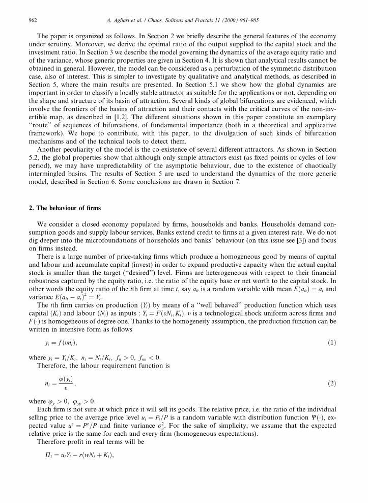
A particular symmetry property is immediately evident from Fig. 1(c). That is, whichever is the attractorwe are considering (at ®nite distance or at in®nity), its basin of attraction is symmetric, as stated in thefollowing:

Property 3 (Symmetry of the basins of T0). Let B be a basin of attraction of an attractor of T0, then B issymmetric with respect to the vertical line of equation:

a � C1

2C2

: �26�

That is, points which are symmetric with respect to (26) are mapped by T0 in the same point. Actuallythis line of symmetry for the basins is a particular line for the map T0. As we shall see below, it belongs to

968 A. Agliari et al. / Chaos, Solitons and Fractals 11 (2000) 961±985

the critical curve LCÿ1 of T0, and is also the line of symmetry of the parabola f, as the critical point Cÿ1 of fhas co-ordinate acÿ1

; acÿ1� C1=2C2:

The proof of Property 3 is easily obtained by using the change of co-ordinate b � aÿ C1=2C2 in (21). Weget a topologically conjugate map:

b0 � ÿC2b2 ÿ C2V � Dÿ 1

4C2

; V 0 � C22 b� ÿ 1�V 2 � 4C2

2b2V �27�

which depends only on b2:We can also investigate whether ``feasible trajectories'' of the map exist. From an applicative point of

view we are interested in bounded trajectories the points of which have V P 0 and a > 0. The secondcondition may probably be obtained if the parameters are such that a�Q � 0. This is not a rigorous proof,but an empirical result, shown in the examples of this paper, which has a theoretical support on the one-dimensional restriction to the a-axis. Moreover, from Property 4 follows that the map is suitable for ap-plications.

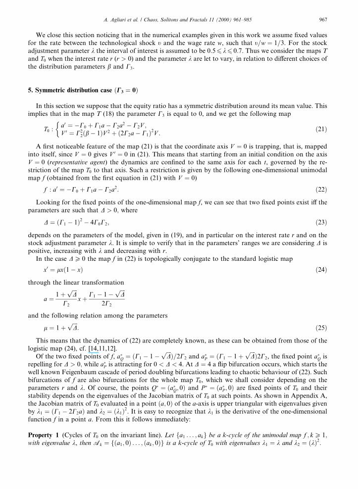
Fig. 1. (a) The critical curve LCÿ1. The values of the parametrs are given in the ®gure. (b) Critical curves LC � T0�LCÿ1�. The regions

Zk represent the set of point having k distinct pre-images. The points of LC�a� have four pre-images, two of which merge on LC�a�ÿ1 ; the

points of LC�b� have four pre-images, two of them merge on the left branch of LC�b�ÿ1 , the other two on the right branch of LC�b�ÿ1 . (c)

Basins of attraction of a 2-cycle attracting node A2 on the a-axis and of the ®xed point R�. The white points belong to the basin B�R��,the dark-grey points denote the basin B�A2� and the light-grey points belong to the basin of in®nity (diverging trajectories). The

repelling ®xed points Q�, P � and S� belong to the boundaries. In the enlargement of (c) the half-fractal structure of the frontier of the

basins is shown, due to the pre-images of any rank of the small area U0 in the region V > 0.

A. Agliari et al. / Chaos, Solitons and Fractals 11 (2000) 961±985 969

Property 4 (Feasible trajectories of T0). Let bP 1. Then a point �a; V � with V > 0 is mapped by T0 into apoint �a0; V 0� with V 0 > 0:

In other words, a point �a; V � having V < 0 cannot have a feasible point as rank-1 pre-image, and thismeans that all its pre-images, of any rank, are in the negative half-plane V < 0. This property is useful tounderstand the global structure of the basins of attraction. Even if we are interested in the portion be-longing to the half-plane V P 0, the changes in the structure of the basins depend on the global propertiesof the map in the whole plane. In particular on the number and position of the rank-1 pre-images of apoint �a0; V 0� by backward application of T0. To this scope we have to determine the critical curves of themap. From the Jacobian matrix given in Appendix A it is easy to see that the locus Det J�a; V � � 0 isgiven by two curves, which represent, in our case, two branches of LCÿ1, that is LCÿ1 � LC�a�ÿ1 [ LC�b�ÿ1

where

LC�a�ÿ1 : a � C1

2C2

and LC�b�ÿ1 : V � C1 ÿ 2C2a� �22C2

2 3ÿ b� � : �28�

The ®rst curve is the symmetry line (26) of the basin, the second one is a parabola with vertex on the a-axis, in the critical point Cÿ1 of the map f. We note that LC�a�ÿ1 intersects the trapping axis in the critical pointCÿ1; while LC�b�ÿ1 is tangent to that axis in Cÿ1 (an example is shown in Fig. 1(a)). The images of these curvesunder the map T0 give the two branches of LC, LC � T0�LCÿ1� � LC�a� [ LC�b�. The branch LC�a� ofequation

LC�a� : V � b� ÿ 1� a�ÿ C2

1 ÿ 4C0C2

4C2

�2

�29�

is a convex parabola, when b > 1, with vertex on the a-axis in the critical point C of the map f, of co-ordinate aC � f �aCÿ1

� � �C21 ÿ 4C0C2�=4C2, while for b � 1 the curve degenerates into the a-axis V � 0. The

branch LC�b� of equation

LC�b� :V � 4

5ÿb aÿ C21ÿ4C0C2

4C2

� �2

a6 aC � C21ÿ4C0C2

4C2

8<: �30�

is a semi-parabola with vertex on the a-axis, again in the critical point C of f, as shown in Fig. 1(b).The portions of phase plane bounded by the critical curves LC�a� and LC�b� are regions Zj, j 2 0; 2; 4f g,

the points of which have j di�erent rank-1 pre-images. This can be seen by computing the rank-1 pre-imagesby �T0�ÿ1

of a generic point of the plane. Given a point p � �a0; V 0�; its rank-1 pre-images are the pointsb� �C1=2C2�; V� � where �b; V � are the real solutions of the algebraic system

ÿC2b2 ÿ C2V � Dÿ 1

4C2

� a0 ÿ C1

2C2

; C22 b� ÿ 1�V 2 � 4C2

2b2V � V 0: �31�

The system (31) may have 0, 2 or 4 solutions, which can be explicitly written, as shown in Appendix B.As a consequence we have that the portion of plane between LC�a� and LC�b� is a region Z4 (see Fig. 1(b)).The region below the curve LC�a� is a region Z2. The remaining portion of plane, bounded by LC�b� and apart of LC�a� (the one on the right of the point C) is a region Z0:

From Fig. 1(c) it is also immediately evident the di�erent structure which characterizes the basins in theregion V > 0 with respect to those in the region V < 0. Besides Property 3 (which is peculiar of the mapunder study), we recall here another important property of any basin of attraction B, that is, the boundary,or frontier, say F � oB, is backward invariant, which means invariant by inverse iterations of the map,including all the di�erent inverses. Thus a frontier F includes the stable sets of all the cycles belonging toF. In Fig. 1(c) the frontier F � oB�1� includes the repelling ®xed points S� (see Appendix A), Q� and P �,and their stable sets. Note that if a point is a repelling node (as Q� for example), then its stable set is givenby the set of all its pre-images of any rank (W s � Sn>0 Tÿn

0 �Q��). The upper boundary of the frontiers ofB�R�� and B�A2� in the region V > 0 have a smooth shape. This is due to the fact that only a few cycles

970 A. Agliari et al. / Chaos, Solitons and Fractals 11 (2000) 961±985

exist on the frontier in the region V > 0 (on which the pre-images of points of the frontiers accumulate),and to the existence of the region Z0 whose points have no pre-images. On the contrary, the frontiers of thetwo basins in the region V < 0 have an ``half-fractal'' structure, i.e. are made up of smooth arcs having aself-similar structure which accumulate on a Cantor set of points which includes repelling cycles of T0 of anyorder. This can be explained as follows. We recall that the whole half-plane V < 0 belongs to Z2, that is, anypoint in this region has two rank-one pre-images, which are one on the right and one on the left of LC�a�ÿ1 , thesymmetry line. For a point p � �a; V � with V < 0, let �T0�ÿ1

1 �p� be the rank-1 pre-image on the right, and�T0�ÿ1

2 �p� the one on the left, of LC�a�ÿ1 . From Property 4 we have that both these rank-1 pre-images are againin the half-plane V < 0. Thus we can iteratively repeat the application of the two inverses �T0�ÿ1

1 and �T0�ÿ12

to all the points so obtained, and also to a portion in this region, noticing that starting from points in B�R��or in B�A2 in the region V < 0 we cannot exit from these basins. This mechanism can be used to show thatin®nitely many repelling cycles of T0, of any order, exist on the boundaries. In particular the ®xed points Q�

and P � on the a-axis have in®nitely many pre-images on the frontiers below the invariant line, and these pre-images also have the ®xed points as limit sets. That is, pre-images of the ®xed points can be found as near tothe ®xed points as we want. This means that both the ®xed points Q� and P � are snap-back-repellers (see[15,13]) and chaotic dynamics exist on the frontiers of the basins (but not inside). It is also easy to computenumerically homoclinic points of Q� and homoclinic points of P �, as the inverses are explicitly known, andwe can choose particular sequences in the arborescent structure of inverses, more suitable to ®nd the ho-moclinic points. For example, consider the rank-1 pre-image Q�ÿ1 � �aQÿ1

; 0� whereaQÿ1� �C1 � 1� ����

Dp �=2C2, then applying iteratively the inverse which gives points on the left,S

n>0�T0�ÿn2 �Q�ÿ1�, we get an homoclinic orbit of Q�. Similarly, considering the rank-1 pre-image of P � on the

a-axis, say P �ÿ1; thenS

n>0�T0�ÿn1 �P �ÿ1� gives an homoclinic orbit of P �. We remark that by repeating iter-

atively any kind of composition of the two inverses �T0�ÿ11 and �T0�ÿ1

2 , all the cycles of any order of thefrontiers can be detected. Although this is not of direct interest in the applicative model under study (forwhich only the basins in the region V > 0 are to be considered), we can give reason of the half-fractalstructure of the basins below the a-axis. The smooth arcs come from the basin B�R��. In the enlargement ofFig. 1(c), an arrow shows a region denoted by U0 above the a-axis, bounded by an arc of critical curve LC�a�

and a portion of oB�R��. The pre-images Uÿ1 � �T0�ÿ11 �U0� [ �T0�ÿ1

2 �U0� give rise to the two regions con-nected on LC�a�ÿ1 ; the two white portions having the shape of a ``crescent''. On its turn the region Uÿ1 has anarborescent sequence of pre-images which gives rise to the half-fractal shape of the frontiers. We use theterm ``half'' in characterizing this kind of frontier because we have the smooth arcs which accumulate in aself-similar shape on a repelling Cantor set. As we shall see in Section 5.2, the absence of smooth arcs givesrise to a ``fractal'' frontier.

5.1. Simply-connected, multiply-connected and disconnected basins

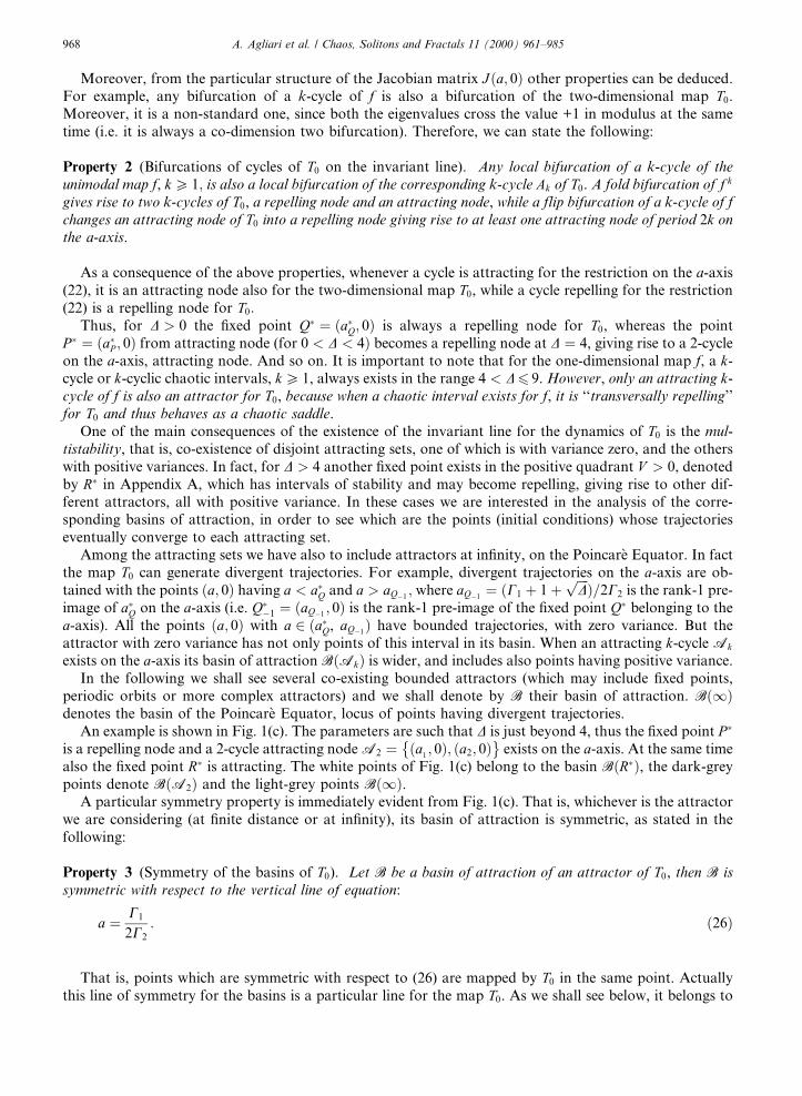
As we can see from Fig. 1(c), the white points belonging to the basin B�R�� in the half-plane V > 0 weare interested in, constitute a simply-connected region, wide enough to consider this case quite suitable foran applicative interpretation, i.e. quite good also from a global point of view. Let us assume, for example,that the state of our system is near the equilibrium R�; which is locally stable. We expect that the phasepoint will converge to the equilibrium, and if some exogenous event (a shock) happens, which changes thestate of the system, putting it not far from the previous state, the basin is wide enough to think that we shallnot go out of the basin of attraction. After the shock the iterations will continue to converge to the stableequilibrium starting from the new position. However the situation is often quite di�erent, and even if a ®xedpoint (or a di�erent attractor) is locally stable, its basin may be not wide and not ``robust'' with respect toperturbations of the state.

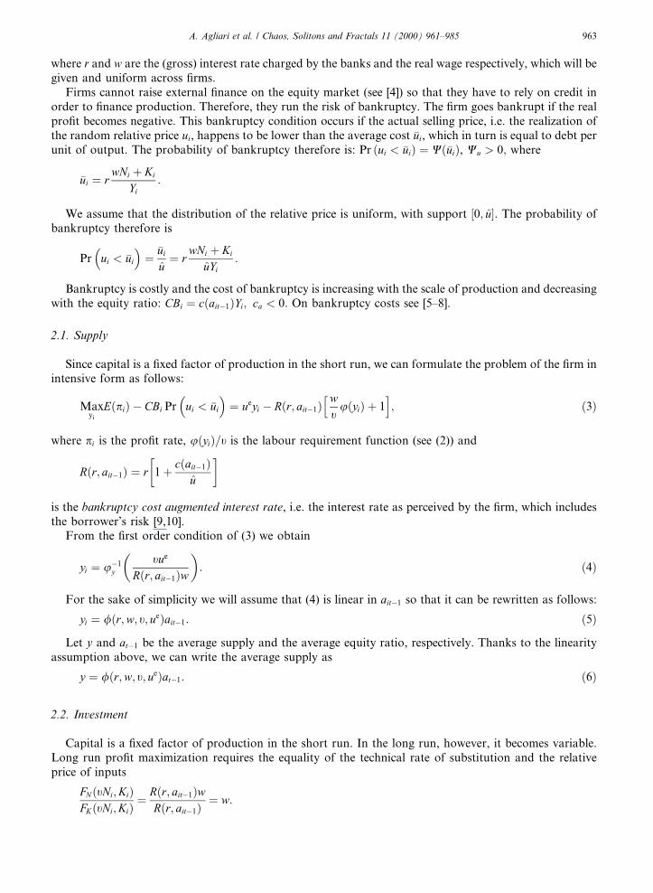
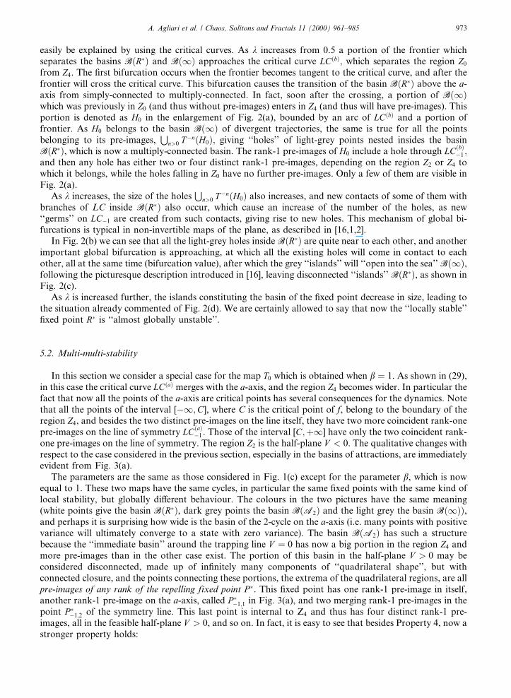
An example is shown in Fig. 2(d), obtained with the same parameter values used in Fig. 1(c) except for asmall increase in the value of k. In Fig. 2(d) the ®xed point R� is still attracting but now the white points(belonging to its basin of attraction) are located in small ``islands'', although in®nitely many in number. It isclear that a small shock applied to a point in the basin B�R�� is likely to bring the point out of the basin,and from the new state the trajectory will be divergent. We remark again that what is changed from thesituation in Fig. 1(c) to that of Fig. 2(d) is only the global structure of the basin B�R�� and not the localcharacter of the ®xed point. On increasing k from 0.5 to 0.57 several global bifurcations occur, which can

A. Agliari et al. / Chaos, Solitons and Fractals 11 (2000) 961±985 971

Fig. 2. Bifurcations of the basin B�R��: (a) After the contact of LC�b� with the portion of frontier which separates the basins B�R�� and

B�1�, the region H0 enters in Z4, as shown in the enlargement. The pre-images of H0 give ''holes'' of light-grey points nested inside the

basin the basin B�R��, which is multiply-connected. (b) The light-grey holes inside B�R�� are increased in size and in number and are all

quite near to each other. (c) After the global bifurcation at which all the existing holes come in contact to each other, B�R�� is made up

of disconnected ``islands''. (d) The ®xed point R� is still attracting but now its basin (the white points) is quite reduced.

972 A. Agliari et al. / Chaos, Solitons and Fractals 11 (2000) 961±985

easily be explained by using the critical curves. As k increases from 0.5 a portion of the frontier whichseparates the basins B�R�� and B�1� approaches the critical curve LC�b�; which separates the region Z0

from Z4. The ®rst bifurcation occurs when the frontier becomes tangent to the critical curve, and after thefrontier will cross the critical curve. This bifurcation causes the transition of the basin B�R�� above the a-axis from simply-connected to multiply-connected. In fact, soon after the crossing, a portion of B�1�which was previously in Z0 (and thus without pre-images) enters in Z4 (and thus will have pre-images). Thisportion is denoted as H0 in the enlargement of Fig. 2(a), bounded by an arc of LC�b� and a portion offrontier. As H0 belongs to the basin B�1� of divergent trajectories, the same is true for all the pointsbelonging to its pre-images,

Sn>0 Tÿn�H0�; giving ``holes'' of light-grey points nested insides the basin

B�R��, which is now a multiply-connected basin. The rank-1 pre-images of H0 include a hole through LC�b�ÿ1 ;and then any hole has either two or four distinct rank-1 pre-images, depending on the region Z2 or Z4 towhich it belongs, while the holes falling in Z0 have no further pre-images. Only a few of them are visible inFig. 2(a).

As k increases, the size of the holesS

n>0 T ÿn�H0� also increases, and new contacts of some of them withbranches of LC inside B�R�� also occur, which cause an increase of the number of the holes, as new``germs'' on LCÿ1 are created from such contacts, giving rise to new holes. This mechanism of global bi-furcations is typical in non-invertible maps of the plane, as described in [16,1,2].

In Fig. 2(b) we can see that all the light-grey holes inside B�R�� are quite near to each other, and anotherimportant global bifurcation is approaching, at which all the existing holes will come in contact to eachother, all at the same time (bifurcation value), after which the grey ``islands'' will ``open into the sea'' B�1�,following the picturesque description introduced in [16], leaving disconnected ``islands'' B�R��, as shown inFig. 2(c).

As k is increased further, the islands constituting the basin of the ®xed point decrease in size, leading tothe situation already commented of Fig. 2(d). We are certainly allowed to say that now the ``locally stable''®xed point R� is ``almost globally unstable''.

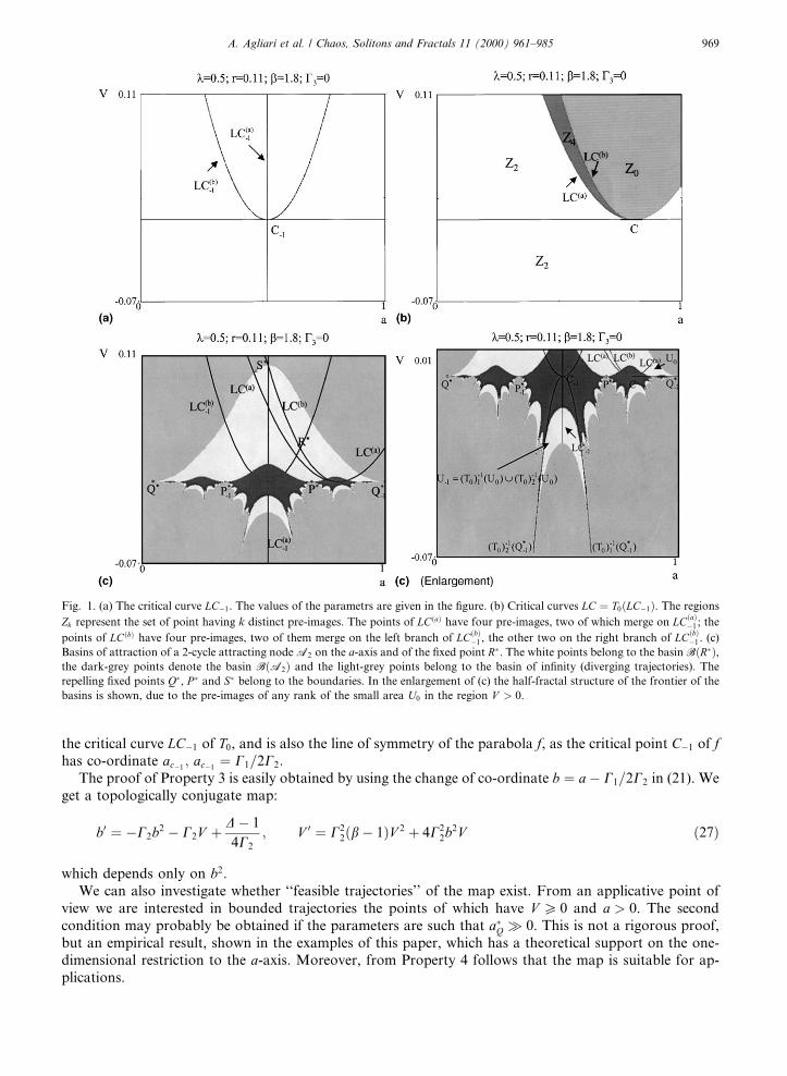
5.2. Multi-multi-stability

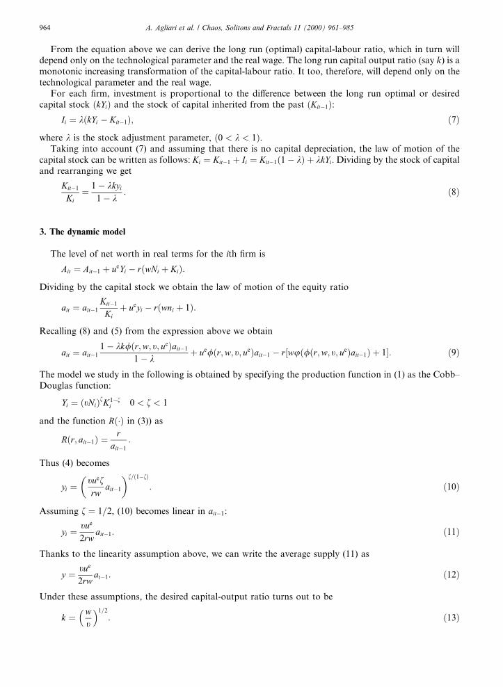
In this section we consider a special case for the map T0 which is obtained when b � 1. As shown in (29),in this case the critical curve LC�a� merges with the a-axis, and the region Z4 becomes wider. In particular thefact that now all the points of the a-axis are critical points has several consequences for the dynamics. Notethat all the points of the interval [ÿ1;C], where C is the critical point of f, belong to the boundary of theregion Z4, and besides the two distinct pre-images on the line itself, they have two more coincident rank-onepre-images on the line of symmetry LC�a�ÿ1 . Those of the interval [C;�1] have only the two coincident rank-one pre-images on the line of symmetry. The region Z2 is the half-plane V < 0. The qualitative changes withrespect to the case considered in the previous section, especially in the basins of attractions, are immediatelyevident from Fig. 3(a).

The parameters are the same as those considered in Fig. 1(c) except for the parameter b, which is nowequal to 1. These two maps have the same cycles, in particular the same ®xed points with the same kind oflocal stability, but globally di�erent behaviour. The colours in the two pictures have the same meaning(white points give the basin B�R��, dark grey points the basin B�A2� and the light grey the basin B�1��,and perhaps it is surprising how wide is the basin of the 2-cycle on the a-axis (i.e. many points with positivevariance will ultimately converge to a state with zero variance). The basin B�A2� has such a structurebecause the ``immediate basin'' around the trapping line V � 0 has now a big portion in the region Z4 andmore pre-images than in the other case exist. The portion of this basin in the half-plane V > 0 may beconsidered disconnected, made up of in®nitely many components of ``quadrilateral shape'', but withconnected closure, and the points connecting these portions, the extrema of the quadrilateral regions, are allpre-images of any rank of the repelling fixed point P �. This ®xed point has one rank-1 pre-image in itself,another rank-1 pre-image on the a-axis, called P �ÿ1;1 in Fig. 3(a), and two merging rank-1 pre-images in thepoint P �ÿ1;2 of the symmetry line. This last point is internal to Z4 and thus has four distinct rank-1 pre-images, all in the feasible half-plane V > 0, and so on. In fact, it is easy to see that besides Property 4, now astronger property holds:

A. Agliari et al. / Chaos, Solitons and Fractals 11 (2000) 961±985 973

Fig. 3. (a) The white points belong to the basin B�R��, the red points denote the basin B�A2� of the 2-cycle on the a-axis, and the grey points B�1�. The

portion of the basin B�A2� in the region V > 0 is made up of in®nitely many components of ``quadrilateral shape'', whose extrema are pre-images of the

repelling ®xed point P �. In the enlargement of (a) it is shown the portion of the basin B�A2� in the region V < 0 which is fractal. (b) A 4-cycle A4

attracting node (marked with stars) exists on the a-axis (born by ¯ip-bifurcation). Other two attracting cycles exist: a 2-cycle A02, marked with circles, just

above the a-axis, and a 4-cycle A04, marked with cross, near the ®xed point R�, now repelling. The points inside the ``old quadrilateral portions'' of Fig.

3(a) now are divided into points belonging to B�A4� and to B�A02�, again in basins having a quadrilateral shape (self-similar structure). (c) There are three

co-existing di�erent attractors, with chaotic dynamics: a 4-band chaotic attractor around the repelling ®xed point R�, a 2-band chaotic attractor near the

a-axis (all in the positive region), and a 4-pieces chaotic attractor having one side on the a-axis. (d) All the chaotic areas of Fig. 3(c) belong to an ab-

sorbing area bounded by the critical arcs LC�b�k � T k0 LC�b�ÿ1

� �, k � 1; 2; . . . ; 7. (e) Single chaotic area, bounded by arcs of LC and LC1.

974 A. Agliari et al. / Chaos, Solitons and Fractals 11 (2000) 961±985

Property 5. Let b � 1 in the map T0. Then all the rank-1 pre-images of a point �a; V � with V > 0 (resp. V < 0)are points belonging to the half-plane V > 0 (resp. V < 0).

As a consequence of this property we have that no white point can exist below the a-axis, that is, thebasin B�R�� of the stable ®xed point is necessarily in the feasible region V > 0:

As already remarked in Section 5, there is a great di�erence in the shape of the frontiers in the two half-planes: those above the a-axis are smooth, and those below are fractal (now true fractal). It is quite evidentthe similarity of the frontier of the basin in the region V < 0 (see the enlargement of Fig. 3(a)) with thefractal set obtained for the basin of the complex map z0 � z2 ÿ 1 (see, for example, [17]). The ®xed points Q�

and P � have homoclinic points, and the same is true for all the in®nitely many repelling cycles on thatfrontier in the region V < 0.

As the parameter r is decreased, we increase the non-linear e�ects in the one-dimensional map f, theattracting 2-cycle undergoes a ¯ip-bifurcation, and an attracting 4-cycle appears. As we know fromProperty 2, this is also a bifurcation for the map T0, of co-dimension two. The result in our case is that the2-cycle A2 turns into a repelling node and a 4-cycle A4 attracting node appears on the a-axis, and, at thesame time, another 2-cycle A0

2 attracting node appears just above the a-axis (bifurcating from A2�.Moreover, also the ®xed point R� becomes unstable, and attracting cycles are created near it. In Fig. 3(b) anattracting 4-cycle, say A0

4, exists near the repelling focus R�. Reassuming, we have three co-existing at-tracting cycles: A0

2 and A04 in the positive half-plane and A4 on the a-axis. Their basin of attraction are

shown in Fig. 3(b). It can be seen that the points inside the ``old quadrilateral portions'' (old basin B�A2��of Fig. 3(a) now are divided into points belonging to B�A4� and to B�A0

2�, again in basins having aquadrilateral shape (self-similar structure), the extrema of which are the pre-images of any rank of therepelling two cycle A2:

As r is further decreased several bifurcations lead to chaotic attractors. In Fig. 3(c) we show a situationin which there are three co-existing di�erent attractors, with chaotic dynamics: a 4-band chaotic attractoraround the repelling ®xed point R�; a 2-band chaotic attractor near the a-axis (but all in the positive re-gion), and a 4-pieces chaotic attractor having one side on the a-axis. As in the one-dimensional case thechaotic intervals are bounded by critical points, in the two-dimensional case we have absorbing areas andchaotic areas bounded by segments of critical curves. Following [1,2], by taking the segment of criticalcurve LC�b�ÿ1 inside the area of the example given in Fig. 3(c), with a few images by T0 we get an invariant areabounded by critical segments, shown in Fig. 3(d). With smaller segments of LC�b�ÿ1 all the distinct pieces ofchaotic areas are bounded by a few critical arcs. Then the chaotic areas increase in size, and shall merge intoa single chaotic piece. An example is shown in Fig. 3(e). It is clear that now the state of the system isunpredictable. However, we can observe that such a state is not ``completely'' unknown, because we knowits width, i.e. the boundary of the chaotic area. It means that even if we cannot predict the state of thesystem we know the possible width of its variations. For the a-values we know the range, say �amin; amax� inwhich it is con®ned, and the same for the values of the variance, V 2 �Vmin; Vmax�; and often this is already agood information.

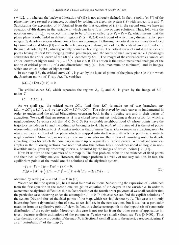
The sequence in Fig. 3 commented above is associated with parameter values of the logistic map insidethe period-2 ``box'' (see the ``box-within-a-box'' bifurcation structure described in [12], or the ``window'' in[14]), and we know that on decreasing r all the boxes associated with any cycle appear. Similar behaviouroccurs also in the positive half-plane: several co-existing attracting cycles may exist, and transition tokÿband chaotic attractors for any natural k. In Fig. 4 we show some situations occurring inside the``period-3 box''.

In Fig. 4(a) we have observed two attractors: a 3-cycle on the a-axis and a 3-cycle around the repellingR�: It is worth noting that inside the area previously occupied by the chaotic attractor now a chaotic re-pellor survives (which are zero-measure invariant sets with chaotic dynamics, containing repelling cyclesand their stable sets) and this is the cause of the complex structure of the basins of the two 3-cycles, asshown in Fig. 4(a) and in its enlargement. Note that although we have only two simple attractors (twocycles of period 3), and a wide set of points with bounded trajectories in the positive half-plane, there areseveral regions in which we cannot predict the asymptotic behaviour for a generic initial condition. In fact,apart from the immediate basins of the two cycles and their ®rst pre-images of low rank, the areas be-longing to the di�erent basins become smaller and smaller accumulating in the points of the repelling

A. Agliari et al. / Chaos, Solitons and Fractals 11 (2000) 961±985 975

Fig. 4. Period-3 box. (a) Basins of two di�erent attractors: a 3-cycle on the a-axis, marked with stars, and a 3-cycle around the repelling

point R�, marked with cross. The areas belonging to the di�erent basins (red and white points) are intermingled in a chaotic (fractal)

way, as shown in the Enlargement. (b) We have four di�erent attractors: a 6-cycle on the a-axis, a 3-cycle just above the a-axis and two

6-cycles with positive variance. Their basins of attraction (white, green, yellow and red points) are chaotically intermingled. All these

cycles belong to the absorbing area bounded by three critical arcs. (c) Two co-existing attractors: a 3-band chaotic attractor in the

region V > 0 and a 3-pieces chaotic attractor having one side on the a-axis. (d) One-piece chaotic attractor, bounded by three arcs of

critical curves. (e) The chaotic area completely ®lls its basin.

976 A. Agliari et al. / Chaos, Solitons and Fractals 11 (2000) 961±985

Cantor sets, and thus are intermingled in a chaotic (fractal) way. Clearly in this situation there is alsounpredictability with respect to an exogenous shock, as perturbing a state we can no longer say whether theasymptotic behaviour will be the same or will change.

As before, when the ¯ip bifurcation of the 3-cycle on the a-axis occurs, giving rise to an attracting 6-cycleon the a-axis, then (due to the bifurcation of both the eigenvalues) also an attracting 3-cycle with positivevariance appears. Moreover, other bifurcations of the two-dimensional map lead to two other di�erent 6-cycles with positive variance, and in the absorbing area of Fig. 4(b) there are such four different attractingsets. It is clear that their basins of attraction are chaotically intermingled.

As expected, we get chaotic regions as r is decreased further. In Fig. 4(c) we have two co-existing chaoticattractors: a 3-band chaotic pieces in the region V > 0 and 3-cyclical chaotic pieces having one side on thea-axis. These will turn into a one-piece chaotic attractor, bounded by three arcs of critical curves, as shownin Fig. 4(d).

On decreasing r for the one-dimensional map f all the dynamics occur, up to D � 9 (i.e. l � 4 in thestandard logistic), and this is the last value at which a bounded invariant interval exists. Similarly, the two-dimensional attracting sets belong to wider and wider absorbing areas, up to this last bifurcation, when thetwo-dimensional chaotic area completely ®lls its basin (as it occurs for the one-dimensional restriction), asshown in Fig. 4(e). Beyond this value the generic trajectory will be divergent.

6. Non-symmetric distribution case �C3 > 0�

In this section we return to consider the complete model, the map T given in (18), in the generic case ofnon-symmetric distribution, which means that the parameter C3 is positive (and small, as already remarkedin Section 4). In this case we loose all the analytical results of Section 5. Only ``guided'' numerical inves-tigations can be used. Being C3 very close to zero, we can consider the map T as a slight perturbation of themap T0 of the symmetric case. This will be evident from the examples described in this section.

We ®rst note that the critical curves can be obtained numerically, by drawing the set Det J�a; V � � 0which gives LCÿ1: This curve now consists of two disjoint branches (perturbations of the two intersectingbranches occurring in the symmetric case). In Fig. 5(a) we consider parameter values close to those used inFigs. 1 and 2 of Section 5.

Besides the critical curve LCÿ1 � LC�a�ÿ1 [ LC�b�ÿ1 also LC � T �LCÿ1� is numerically computed, and its twobranches are shown in Fig. 5(a). The branch LC�a� has a cusp point while the branch LC�b� has a parabolicshape. Moreover we compute numerically the distinct rank-1 pre-images of a point of the plane ®nding thatthe area enclosed by the critical curve LC�a� is a region Z4; the region above LC�b� is Z0 and the remainingregion is Z2:

Also the ®xed points are numerically computed, solving the system in (20), which has four real solutions,called R�, Q�; P � and S� in Fig. 5(a). Only R� is locally stable, the other three ®xed points belong to thefrontier F which separates the basin of R� from the points having divergent trajectories (i.e.F � oB�R�� � oB�1��. Now the a-axis is no longer invariant, however we can still observe two di�erentqualitative structures in the shape of F. The lower part between Q� and Q�ÿ1 (completely in Z2� has still anhalf-fractal shape, which can be explained by using arguments similar to those used in Section 5. Whereasthe upper part of F has a smooth shape. The grey points of Fig. 5(a) give the basin B�1�, while the whiteregion is the locus of points having bounded trajectories. As besides the ®xed point R� we have not observedany other attracting set for T, we assume that the white region is B�R��.

The dynamic behaviour of T as the parameters are varied from the case of Fig. 5(a) are very similar tothose observed in the symmetric case. Either increasing k or decreasing r the global bifurcations of the basinof bounded trajectories occur, due to contacts with the critical curves, changing the simply-connected basininto a multiply-connected and then into a disconnected one. The only di�erence is in the attracting setwhich, instead of the ®xed point R�, may be a closed invariant curve C� born at the supercritical Neimark±Hopf bifurcation of R� (turned into repelling focus). In Fig. 5(b) we can see such closed invariant attractingcurve C� (we have chosen to show what occurs on decreasing r). A contact bifurcation between F and thecritical curve LC�b�, causing the ®rst global bifurcation of the basin, has already occurred, and then thecrossing creates a portion H0 of the basin B�1� which belongs now to Z2 (previously in Z0�, see the

A. Agliari et al. / Chaos, Solitons and Fractals 11 (2000) 961±985 977

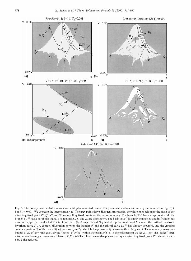
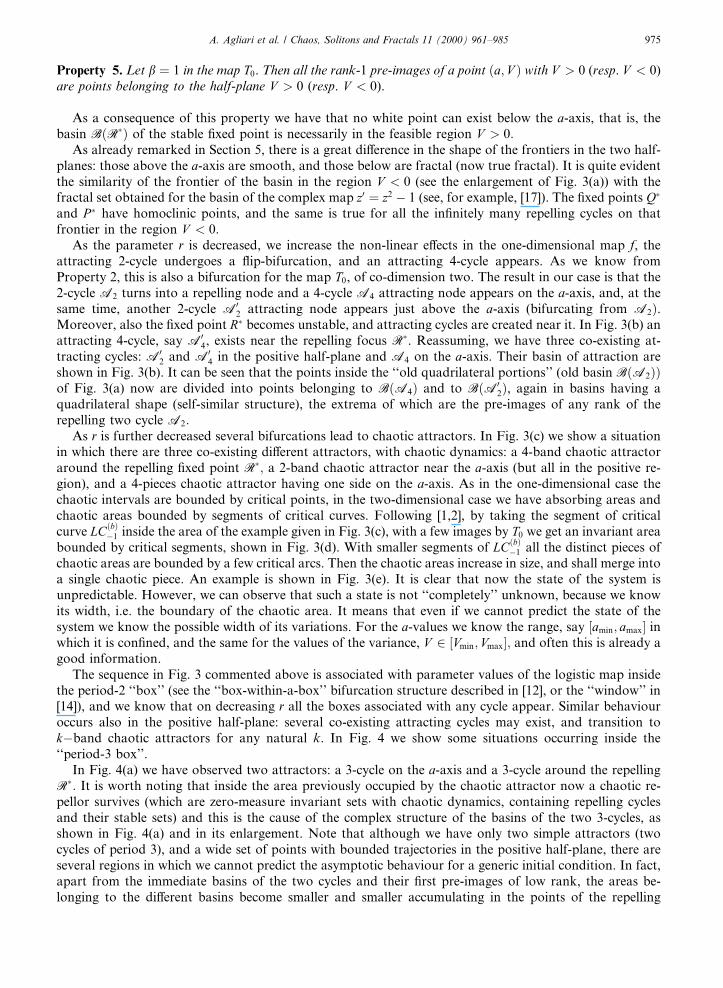
Fig. 5. The non-symmetric distribution case: multiply-connected basins. The parameters values are initially the same as in Fig. 1(c),

but C3 � 0:001. We decrease the interest rate r. (a) The grey points have divergent trajectories, the white ones belong to the basin of the

attracting ®xed point R�. Q�, P � and S� are repelling ®xed points on the basin boundary. The branch LC�a� has a cusp point while the

branch LC�b� has a parabolic shape. The regions Z0, Z2 and Z4 are also shown. The basin B�R�� is simply-connected and its frontier has

a smooth upper part and a half-fractal lower part. (b) A supercritical Neymark±Hopf bifurcation of R� caused the birth of the closed

invariant curve C�. A contact bifurcation between the frontier F and the critical curve LC�b� has already occurred, and the crossing

creates a portion H0 of the basin B�1�, previously in Z0; which belongs now to Z2; shown in the enlargement. Then in®nitely many pre-

images of H0 of any rank exist, giving ``holes'' of B�1� within the basin B�C��. In the enlargement we see Hÿ1. (c) The ''holes'' open

into the sea, leaving a disconnected basins B�C��. (d) The closed curve disappears leaving an attracting ®xed point R�, whose basin is

now quite reduced.

978 A. Agliari et al. / Chaos, Solitons and Fractals 11 (2000) 961±985

enlargement of Fig. 5(b). Then in®nitely many pre-images of H0 of any rank exist, giving ``holes'' of B�1�within the basin B�C��. As r is decreased further the holes increase in size as well as in number, due to othercontacts of the boundaries of the holes with the branches of critical curves LC�a� and LC�b� inside the basinB�C��. The holes will then approach each other until a global bifurcation occurs, at which all of them willcome in touch and then ``the holes will open into the sea'', leaving a disconnected basin B�C��. An exampleis shown in Fig. 5(c). A particular behaviour is now observed on decreasing r: the closed invariant attractingcurve C� decreases in size, approaching the repelling focus R�; and a ``reverse'' Neimark±Hopf bifurcationoccurs: the closed curve disappears leaving an attracting ®xed point R�: In Fig. 5(d) we are in such a sit-uation. Note that now the immediate basin of R�; say B0�R��, (i.e. the simply connected area of the basinincluding the attracting set) is very small, and on its frontier there is only the saddle S�: We argue that thefrontier oB0�R�� of the immediate basin is the local stable set of the saddle S�; and then the total basin ismade up of all its pre-images of any rank, B�R�� � Sn P 0 Tÿn�B0�R���, which are in®nitely many (even ifonly a few of them can be observed in Fig. 5(d)), and accumulating on all the existing repelling cycles of T.

Comparing the dynamics of the map in the cases shown in Fig. 5(a) and (d), where T has a uniqueattracting set, the stable ®xed point R�; we are led to comments similar to those presented in Section 5.1.Attention must be paid when only the local stability of an attractor is analyzed, because we may be in aglobally robust situation as that of Fig. 5(a) or in a situation in which the locally stable ®xed point may beconsidered as almost globally unstable, as that in Fig. 5(d).

We end the comments of this example by noticing that if r is further decreased, the ®xed point R� (whichturns into an attracting node) and the saddle S� will come close to each other, and will merge together at a``reverse'' saddle-node bifurcation which make disappear these two ®xed points. Then the generic trajectoryhas been observed to be divergent.

Finally we close this section showing the dynamics of T when we perturb the particular case presented inSection 5.2, considering C3 � 0:001. In Fig. 6(a) the numerically computed critical curves LCÿ1 and LC aredrawn, each of which is made up of two distinct branches, and also the ®xed points R�; Q�; P � and S�. Asabove, only R� is locally stable while the other three ®xed points belong to the frontier F which separatesthe basin of R� from the points having divergent trajectories.

Also now the area enclosed by the critical curve LC�a� is a region Z4; the region above LC�b� is Z0 while Z2

is the remaining region. We can observe that Z4 is a wide region (a perturbation of the one in Fig. 3(a)), andnow it includes the ®xed point Q�: Then this ®xed point has four distinct rank-1 pre-images, one in itself andthe points Q�ÿ1;1; Q�ÿ1;2; Q�ÿ1;3 shown in Fig. 6(a), the last two of which belong to Z0 and have no other pre-images, while Q�ÿ1;1 belongs to Z2 and has an arborescent sequence of pre-images, located in the lower partof F (where F appears to be half-fractal). In fact, as in the previous case, F is made up of two parts withdi�erent structures, the lower part between Q� and Q�ÿ1;1 which has an half-fractal shape, and the upper partwhich is smooth.

Again the multistability, which was a characteristic of the symmetric case, is lost after the symmetry-breaking, and we don't observe any other attractor besides the ®xed point R�; or the attracting set bifur-cated from that point. Thus the white points of Fig. 6(a) are assumed to give B�R��, while those in Fig. 6(b)belong to B�C��, where C� is an attracting closed invariant curve born via Neimark±Hopf bifurcation fromR�; on increasing k: In the enlargement of Fig. 6(b) we see that the frontier F , after a tangency with thelower branch of LC�a� crosses LC�a� and a portion H0 of the basin B�1�, previously in Z2, now belongs to Z4,giving rise to a couple of new pre-images, one on the right and one on the left of LC�a�ÿ1 , together constitutingthe hole Hÿ1: Thus the contact bifurcation of the frontier has caused the transition of the basin of boundedtrajectories from simply-connected to multiply-connected, although now we have only one hole Hÿ1 (be-cause Hÿ1 belongs to the region Z0 and thus it has no other pre-images).

As k is increased, frequency locking on the closed curve leads to an attracting 4-cycle for T and sequencesof ¯ip-bifurcations give rise to a 4-band chaotic attractor, belonging to an absorbing area of annular shape,and a contact bifurcation of the four pieces causes their reunion into a single chaotic attractor, as shown inFig. 6(c). In the enlargement of that ®gure we see that the absorbing area is bounded by segments of criticalcurves LC�b�; LC�b�1 ; . . . ; LC�b�6 , obtained by iterating the small piece of arc of LC�b�ÿ1 which crosses that area.

In Fig. 6(c) we can also see that the hole Hÿ1 is increased in size and now crosses LC�b�, thus a smallportion of this hole enters Z2, giving rise to new pre-images, called Hÿ2 in that ®gure, but Hÿ2 belongs to theregion Z0 and thus it has no other pre-images. However, the number of holes in the basin of bounded

A. Agliari et al. / Chaos, Solitons and Fractals 11 (2000) 961±985 979

Fig. 6. Chaotic attractors in the non-symmetric case. As in Figs. 3 and 4, we set b � 1, but C3 � 0:001. Chaotic attracting areas are obtained by in-

creasing k. (a) R� is locally stable. The region Z4 now is wider with respect to that of Fig. 5(a) and contains the ®xed points Q�. The points Q�ÿ1;1; Q�ÿ1;2;

Q�ÿ1;3 are the rank-1 pre-images of Q�. Q�ÿ1;1 belongs to Z2 and has an arborescent sequence of pre-images, located in the lower part of the frontier F

(where F appears to be half-fractal). In fact, as in the previous case, F is made up of two parts with di�erent structures, the lower part between Q� and

Q�ÿ1;1 which has an half-fractal shape, and the upper part which is smooth. (b) C� is an attracting closed invariant curve born via Neimark±Hopf bi-

furcation from R� and the white points belong to its basin. In the Enlargement we see that the frontier F, after a tangency with the lower branch of LC�a�

crosses LC�a� and a portion H0 of the basin B�1�, previously in Z2, now belongs to Z4, giving rise to the hole Hÿ1. Now we have only one hole Hÿ1 (because

Hÿ1 belongs to the region Z0 and thus it has no other pre-images). (c) Absorbing area of annular shape. In the Enlargement we see that the absorbing area

is bounded by segments of critical curves LC�b�; LC�b�1 ; . . . ; LC�b�7 , obtained by iterating the small piece of arc of LC�b�ÿ1 which crosses that area.

980 A. Agliari et al. / Chaos, Solitons and Fractals 11 (2000) 961±985

trajectories is increasing also due to new contacts of F with the lower part of LC�a�, which is more clearlyvisible in the enlargement of Fig. 7(a).

Here we see that sequences of bifurcations in the attracting sets have led to a chaotic area, againbounded by a few segments of critical curves LC�b�j . As k is further increased the chaotic area crosses alsoLC�a�ÿ1 and the boundary of the chaotic area now includes also segments of LC�a�j : Also the holes approachand cross the upper branch of LC�a� having a portion which, from Z2; enters Z4 giving rise to new pre-images. The appearance of a portion of the hole Hÿ1 in the region Z4 is a bifurcation with more conse-quences than the previous ones because now the pre-images of any rank of this portion are not ®nite innumber, but in®nitely many, even if only a few of them are visible in Fig. 7(b) (for example, an in®nitesequence of pre-images exists which gives smaller and smaller holes approaching the ®xed point Q� insidethe region Z4�:

Several bifurcations are observed in the attracting sets on varying k, appearance of boxes of stable cyclesand their routes to chaos, and explosions in wider chaotic areas. In the last ®gure, Fig. 7(c), we see that thechaotic area is now very close to the frontier of its basin. As in fact a contact will occur, causing thetransition of that chaotic attractor into a chaotic repellor, after which the generic trajectory is observed tobe divergent. However, we remark that this example corresponds to what is generally observed in

Fig. 7. Chaotic attractors of di�erent shapes in the non- symmetric case with b � 1. (a) The number of ''holes'' in the basin of bounded

trajectories is now increased. In the enlargement the new contacts of the frontier F with LC�a� are shown. The chaotic area is bounded

by a few segments of critical curves LC�b�j . (b) The chaotic area crosses also LC�a�ÿ1 and the boundary of the chaotic area now includes

also segments of LC�a�j . Due to the crossing of Hÿ1 with the region Z4 now the grey holes are in®nitely many. (c) The chaotic area is now

very close to the frontier of its basin.

A. Agliari et al. / Chaos, Solitons and Fractals 11 (2000) 961±985 981

two-dimensional non-invertible maps, in which the contact between an invariant chaotic area and theboundary of its basin occurs when the invariant area has not completely ®lled the basin (di�erently fromwhat was exceptionally found in the example shown in Fig. 4(e)). In this generic case it is very di�cult tounderstand whether some attracting set survives or not. A cycle of high period and very small basin ofattraction may exist, not only after the contact, but also in the case shown in Fig. 7(c), although it isnumerically not detectable. However, we also note that such cases are of less importance from an appli-cative point of view, where the generic behaviour is considered as representative of the dynamics of thesystem.

7. Conclusions

The model of ¯uctuating growth presented in this paper gives rise to several kinds of dynamic behav-iours. Although almost analytically intractable, we have shown how several dynamical properties can beexplained by using theoretical arguments coupled with numerical tools. The global bifurcations of thebasins of attractions described in Sections 5 and 6 show that local stability is often not enough to consider amodel as stable or suitable for the applications. Whereas the arguments in Section 5.2 show that we mayhave di�erent co-existing attractors whose basins have complex structures, which gives rise to the unpre-dictability of the asymptotic behaviour for a generic point in the region of interest.

The cases we have considered certainly do not cover all the possible dynamics. However, by applying thetechniques which make use of the global basins and of the critical curves, as described in Sections 5 and 6,we hope that other kinds of dynamics can be explained, both locally and globally, as well as new bifurcationmechanisms.

From an applicative point of view we are led to be cautions with our models. Given a situation whichde®nes the parameters' values, we can describe the time evolution and realize if we are in a stable regime orin a regime with oscillatory cycles or in a complex one, and whether particular attention must be paid tosmall perturbations, which may drastically change the time evolution. We hope that the knowledge of theparameters' regimes, specially those ``more critical'' for the dynamics, may be of help also to guide theoperators.

Acknowledgements

The work has been performed under the activity of the national research project ``Dinamiche non-lineariedapplicazioni alle scienze economiche e sociali'', MURST, Italy and under the auspices of CNR, Italy.

Appendix A

In this appendix we consider the map T0 in (21) and determine its ®xed points, solutions of the algebraicsystem (21) with C3 � 0, that is

ÿC0 � C1 ÿ 1� �aÿ C2a2 ÿ C2V � 0;

V �C22�bÿ 1�V � 2C2aÿ C1� �2 ÿ 1� � 0:

�A:1�

As observed in Section 5, the a-axis is trapping for the map T0, and the restriction to this axis is conjugatedto the standard logistic map. Thus, assuming D > 0, where D � �C1 ÿ 1�2 ÿ 4C0C2, two ®xed points are onthe a-axis, say Q� and P �. The solutions obtained with V � 0 in the ®rst equation of (A.1),a�Q � �C1 ÿ 1ÿ ����

Dp �=2C2 and a�P � �C1 ÿ 1� ����

Dp �=2C2; give the two ®xed points of the map T0:

Q� � C1 ÿ 1ÿ ����Dp

2C2

; 0

!and P � � C1 ÿ 1� ����

Dp

2C2

; 0

!: �A:2�

Two other ®xed points exist.

982 A. Agliari et al. / Chaos, Solitons and Fractals 11 (2000) 961±985

· For b > 1, substituting V � 1ÿ �2C2aÿ C1�2�=C22�bÿ 1� in the ®rst equation we get, after rearranging,

c0 � c1a� c2a2 � 0, where c0 � ÿ1� C21 ÿ C0C2�bÿ 1�, c1 � C2�C1 ÿ 1��bÿ 1� ÿ 4C1C2; c2 � C2

2�5ÿ b�,which gives the values a�S � �ÿc1 ÿ

��������������������c2

1 ÿ 4c0c2

p �=2c2 and a�R � �ÿc1 ���������������������c2

1 ÿ 4c0c2

p �=2c2; thus the two®xed points of the map T0 are:

S� � a�S ; V�

S

ÿ �and R� � a�R; V

�R

ÿ �; �A:3�

where V � � �1ÿ �2C2a� ÿ C1�2�=�C22�bÿ 1��.

· For b � 1, from the second equation in (A.1) we get a�S � �C1 ÿ 1�=2C2 and a�R � �C1 � 1�=2C2, and byusing the ®rst equation we obtain:

S� � C1 ÿ 1

2C2

;D

4C22

!and R� � C1 � 1

2C2

;Dÿ 4

4C22

!: �A:4�

The local stability of the ®xed points depends on the eigenvalues of the Jacobian matrix of (21) givenby

J a; V� � � C1 ÿ 2C2a ÿ C2

ÿ4C2 C1 ÿ 2C2a� �V C1 ÿ 2C2a� �2 � 2C22�bÿ 1�V

� ��A:5�

evaluated at the ®xed points. In points belonging to the a-axis the matrix J is upper triangular with ei-genvalues given by k1 � C1 ÿ 2C2a and k2 � �k1�2. With a � a�Q and a � a�P we have the eigenvalues as-sociated with the ®xed points on the a-axis. Hence Q� is a repelling node, being k1�Q�� � 1� ����

Dp

witheigenvectors r1�Q�� � 1; 0� �, along the a-axis, and k2 � 1� ����

Dpÿ �2

, with eigenvectorr2�Q�� � �1;ÿ��

����Dp �1� ����

Dp ��=C2��, whereas P � has eigenvalues given by k1�P �� � 1ÿ ����

Dp

, with eigendi-rection along the a-axis, and k2�P �� � �1ÿ

����Dp �2, with eigenvector r2�P �� � �1; �

����Dp �1ÿ � ����Dp ��=C2��. For

0 < D < 4; P � is an attracting node, becoming a repelling node for D > 4. The bifurcation occurring atD � 4 is of co-dimension two, having both the eigenvalues equal to 1 in absolute value. It is a ¯ip bifur-cation along the a-axis, creating a cycle of period 2, attracting node not only for the one-dimensional re-striction but also for the whole map T0, while in the transverse direction the bifurcation is associated withthe eigenvalues +1. Below we shall comment it in the case b � 1.

It is worth noting that for the restriction of the map T0 to the a-axis, given in (22), we know all thedynamics, being that of the logistic map, and from the structure of the Jacobian matrix, upper triangular onthe a-axis, the property stated above regarding the two eigenvalues holds for any cycle.

Regarding the local stability of the other ®xed points, we consider only the case with b � 1 for which wehave simpler explicit solutions. Evaluating the Jacobian matrix (A.5) at S� we have:

J S�� � � 1 ÿ C2

ÿ DC2

1

� �: �A:6�

The matrix (A.6) has real eigenvalues for D > 0, given by k1�S�� � 1� ����Dp

with eigenvectorr1�S�� � 1;ÿ ����

Dp

=C2

ÿ �, and k2�S�� � 1ÿ ����

Dp

with eigenvector r2�S�� � 1;����Dp

=C2

ÿ �. Therefore, for

0 < D < 4; S� is a saddle point, with local stable manifold tangent to r2 and the unstable one tangent to r1;while for D > 4 the saddle becomes a repelling node, via ¯ip-bifurcation (the eigenvalue k2 crosses throughÿ1), creating a 2-cycle saddle.

For the local stability of R� we consider the Jacobian matrix

J R�� � � ÿ1 ÿ C2Dÿ4C2

1

� �

A. Agliari et al. / Chaos, Solitons and Fractals 11 (2000) 961±985 983

which has real opposite eigenvalues if D < 5, being k1�R�� �������������5ÿ Dp

and k2�R�� � ÿ������������5ÿ Dp

, and complexones, with real part 0 (i.e. pure imaginary), otherwise. Hence R� is a repelling node for D < 4, an attractingnode for 4 < D < 6, and a repelling focus for D > 6.

The bifurcation occurring at D � 4 corresponds to a ''change of stability'', as in fact the ®xed points P �

and R� merge at this bifurcation value. The ®xed point R� from the half-plane V < 0 for D < 4, and un-stable, enters the half-plane V > 0 for D > 4 becoming an attracting node.

The bifurcation occurring at D � 6 is a resonant Hopf bifurcation associated with the two eigenvalues +iand ÿi (i being the imaginary unit).

Appendix B

In this appendix we consider the rank-1 pre-images of the map T0 in Eq. (21). Given a generic point ofthe plane, p � �a0; V 0�, then its rank-1 pre-images are the points �b� �C1=2C2�; V � where �b; V � are the realsolutions of the algebraic system in (31), which we rewrite for convenience:

ÿC2b2 ÿ C2V � Dÿ 1

4C2

� a0 ÿ C1

2C2

; C22 b� ÿ 1�V 2 � 4C2

2b2V � V 0: �B:1�

From the ®rst equation of (B.1) we can write

b2 � ÿV � Dÿ 1

4C22

� C1 ÿ 2C2a0

2C22

�B:2�

and substituting into the second equation of (B.1) we get a quadratic equation inV : ÿV 0 � a1V � a2V 2 � 0, where a1 � Dÿ 1� 2�C1 ÿ 2C2a0� and a2 � C2

2 bÿ 5� �. It follows that whenr � �a2

1 � 4a2V 0� < 0 then the point p has zero rank-1 pre-images. While for r > 0 then two values for Vexist, given by V � Vÿ � �ÿa1 ÿ

���rp �=2a2 and V � V� � �ÿa1 �

���rp �=2a2, which are to be substituted in

(B.2). Thus two solutions (i.e. two rank-1 pre-images of p) are get if ÿ Vÿ � Dÿ 1

4C22

� C1 ÿ 2C2a0

2C22

!> 0

and two more pre-images if ÿ V� � Dÿ 1

4C22

� C1 ÿ 2C2a0

2C22

!> 0:

References

[1] C. Mira, L. Gardini, A. Barugola, J.C. Cathala, Chaotic Dynamics in Two-Dimensional Non-Invertible Maps, World Scienti®c,

Singapore, 1996.

[2] R. Abraham, L. Gardini, C. Mira, Chaos in Discrete Dynamical Systems (a Visual Introduction in Two-Dimension), Springer,

Berlin, 1997.

[3] D. Delli Gatti, M. Gallegati, Financial fragility, ¯uctuations and growth, beyond the representative agent, mimeo, 1998.

[4] S. Myers, N. Majluf, Corporative ®nancing and investment decisions when ®rms have informations that investors do not have,

J. Financial Econom. 13 (1984) 187±221.

[5] R. Gordon, B. Malkiel, Corporation ®nance, in: H. Aaron, J. Pechman (Eds.), How Taxes A�ect Economic Behaviour, Brooking

Institution, Washigton, DC, 1981.

984 A. Agliari et al. / Chaos, Solitons and Fractals 11 (2000) 961±985

[6] E. Altman, A further empirical investigation of the bankruptcy cost question, J. Finance 39 (1984) 1067±1089.

[7] S. Gilson, Bankruptcy, boards, band and blockholder: evidence on changes in corporate ownership an control when ®rms default,

J. Financial Econom. 27 (1990) 355±388.

[8] S. Kaplan, D. Reishus, Outside directorship and corporate performance, J. Financial Econom. 27 (1990) 389±410.

[9] J.M. Keynes, The General Theory of Employment, Interest and Money, Macmillan, London, 1936.

[10] H. Minsky, John Maynard Keynes, Columbia University Press, New York, 1975.

[11] I. Gumowski, C. Mira, Dynamique Chaotique, Cepadues Editions, Toulose, 1980.

[12] C. Mira, Chaotic Dynamics, World Scienti®c, Singapore, 1987.

[13] L. Gardini, Homoclinic bifurcations in n-dimensional endomorphisms, due to expanding periodic points, Non-linear Analysis,

T.M.A. 23 (1994) 1039±1089.

[14] P. Collet, J.P. Eckmann, Iterated maps on the interval as dynamical systems, Birkh�auser, Boston, 1980.

[15] F.R. Marotto, Snap-back repellers imply chaos in Rn, J. Math. Anal. Appl. 63 (1978) 199±223.

[16] C. Mira, D. Fournier-Prunaret, L. Gardini, H. Kawakami, J.C. Cathala, Basin bifurcations of two-dimensional non-invertible

maps: fractalization of basins, Int. J. Bifurcation and Chaos 4 (2) (1994) 343±381.

[17] R.L. Devaney, An Introduction to Chaotic Dynamical Systems, The Benjamin/Cummings, Menlo Park, CA, 1987.

A. Agliari et al. / Chaos, Solitons and Fractals 11 (2000) 961±985 985