A coupled mesoscale–microscale framework for windresource estimation and farm aerodynamics

Harish Gopalan a,n, Christopher Gundling a, Kevin Brown a, Beatrice Roget a,Jayanarayanan Sitaraman a, Jefferey D. Mirocha b, Wayne O. Miller b

a Wind Energy Research Center, University of Wyoming, 1000 E. University Avenue, Laramie, WY 82071, USAb Lawrence Livermore National Laboratory, 7000 East Avenue, Livermore, CA 94550, USA

a r t i c l e i n f o

Article history:Received 22 August 2013Received in revised form1 April 2014Accepted 1 June 2014

Keywords:Overset gridsMesoscale microscale couplingLillgrund wind farmWind turbine aerodynamicsWind resource estimation

a b s t r a c t

This study discusses the development of a coupled mesoscale–microscale framework for wind resourceestimation and farm aerodynamics. WINDWYO is a computational framework for performing coupledmesoscale–microscale simulations. The framework is modular, automated and supports coupling ofdifferent mesoscale and microscale solvers using overset or matched grids. The modular nature of theframework and the support for overset grids allows the independent development of mesoscale andmicroscale solvers and the efficient coupling between the codes. The performance of the framework isevaluated by coupling Weather Research and Forecasting (WRF) model with three microscale computa-tional fluid dynamics (CFD) codes of varying complexity. The solvers used are: (i) UWake: a bladeelement model with free-vortex wake, (ii) Flowyo: large eddy simulation code with actuator line/diskparametrization of the wind turbine and (iii) HELIOS: detached eddy simulation code with full rotormodeling and adaptive mesh refinement. Power predictions and wake visualization of single turbine andoff-shore Lillgrund wind farm in uniform and turbulent inflow are used to demonstrate the capabilitiesof the framework.

& 2014 Elsevier Ltd. All rights reserved.

1. Introduction

The prediction of the expected power generation and wakeevolution in a wind farm is a complex fluid–structure interactionproblem which involves interaction between the atmosphericboundary layer (ABL) in the wind farm due to global windpatterns, effect of the upstream local terrain on the wind flowpattern in the farm, turbulent boundary layer on the wind turbineblades and structural vibrations of the entire framework. Thesimulations are further complicated due to the multi-scale spa-tio-temporal turbulence interactions. The length scales in theatmosphere are of the order of several meters and can last forseveral minutes. On the other hand, the size of the turbulentboundary layer on the turbine blades are of the order of fewmicro-meters and the turbulent eddies have life time of fewseconds. A reliable tool for the prediction of the aerodynamicsand power in a wind farm needs to account for these differentscales. However, the current wind farm design tools have

numerical inaccuracies of the order of 10–20% for a single turbine(Gundling et al., 2011, 2012; Rai et al., 2012). Hence, furtherimprovements of the existing methods are required to providean efficient numerical tool for studying the flow in a wind farmand prediction of the performance of the wind turbines.

There are three different methods which have been used forthe investigation of wind farms: (i) upscaling, (ii) downscaling or(iii) coupled methods. The upscaling of a microscale code (Fockenet al., 2001) (adding numerical capability to predict the atmo-spheric wind pattern) or downscaling of a mesoscale code(Yu et al., 2006; Zajaczkowski et al., 2011) (addition of capabilityto predict wind turbine aerodynamics) is clearly not the optimumsolution for this problem due to the multi-scale nature of theproblem and the different algorithmic requirements at the differ-ent scales. The use of a coupled approach allows the simulation ofthe ABL and wind farm separately using their respective algo-rithms and the information is exchanged between both the solversusing some form of numerical interpolation. The coupling can be aone-way data transfer from the mesoscale code to the microscalecode as a boundary condition (Churchfield et al., 2012; Troldberg,2008; Gundling et al., 2012) or body force term (Troldborg et al.,2007) or a two-way data transfer between both the codes (Moenget al., 2007). This coupled method is more general than the

Contents lists available at ScienceDirect

journal homepage: www.elsevier.com/locate/jweia

Journal of Wind Engineeringand Industrial Aerodynamics

http://dx.doi.org/10.1016/j.jweia.2014.06.0010167-6105/& 2014 Elsevier Ltd. All rights reserved.

n Corresponding author: Union College Mechanical Engineering, 218 SteinmetzHall, 807 Union Street, Schenectady, NY 12308, USA.

E-mail address: harish.gopalan@gmail.com (H. Gopalan).

J. Wind Eng. Ind. Aerodyn. 132 (2014) 13–26

upscaling/downscaling procedure using a monolithic code frame-work and has many advantages. First, there are no restrictions onthe choice of the mesoscale or microscale solver. The atmosphericwind speed can be provided either using synthetic turbulence(Mann, 1994; Troldborg et al., 2007; Jonkman, 2009) or realisticsimulations using Weather Research and Forecasting (WRF) orother atmospheric codes. Second, the codes can be developedindependently. The only requirement is that the coupling proce-dure needs to be able to handle the data from both the codes in anautomated and efficient fashion with little user intervention.Numerical computations using such coupled approaches havebeen demonstrated to work successfully in the literature for windenergy applications (Troldborg et al., 2007; Churchfield et al.,2012; Troldberg, 2008; Gundling et al., 2012). However, there aremany issues regarding this coupling which are yet to be resolved.The mesoscale solver can be run using RANS or LES methods. Thecoupling procedure has to be modified based on the turbulencemodeling approach used in the mesoscale solver. The RANSmethods do not provide any unsteady turbulent flow structuresand synthetic turbulence (Mann, 1994; Troldborg et al., 2007;Jonkman, 2009) is required to create the unsteady inflow for themicroscale LES. If LES methods are used in the mesoscale code, thesubgrid scale (SGS) turbulent kinetic energy (TKE) has a muchhigher value because of the coarse grid resolutions while thisvalue is small in the micro scale solver due to the relatively finergrids. Consequently, the subgrid scale turbulent kinetic energy/viscosity cannot be interpolated from one solver to the other inLES and a procedure is required for correctly calculating thisquantity (Moeng et al., 2007). These problems are further compli-cated if hybrid RANS–LES methods are used in either of the codes.All these factors coupled with added difficulty for complex terrainsmake it essential to further investigate and improve the couplingalgorithms.

The one-way coupling approach often involves performing theatmospheric RANS/LES simulations and saving the flow field datafor a specific number of time steps. Single or multiple slices ofvelocity flow field from the mesoscale simulations at each timestep are used as the boundary condition or body force term in themicroscale solvers. A weighted linear interpolation is often used tointerpolate the data between the codes and also between timesteps. The coupling method usually requires that the grids matchat the boundaries for the interpolation of data. This may requireadditional modification to the existing algorithms to couple codeswith different storage paradigms (collocated or staggered grid,cell-centered or vertex centered, etc.) and may reduce the speedand efficiency of the computations.

The current study proposes and discusses the development ofWINDWYO: an overset coupling strategy for using multiple codesin a modular, efficient, and flexible fashion. An overset domainconnectivity assembly is used for coupling the mesoscale andmicroscale codes. The use of this approach mitigates the require-ment of having to match the grids between the different codes.In addition, it is relatively straight forward to couple any mesoscalecode with any microscale code without concern about the gridstructure, flow variable storage, etc. The overset assembly is paralleland fully automated. The simulations can be performed automati-cally with no user intervention. The interpolation of data betweenthe codes is also straight forward. This framework also includes thetraditional coupling method as a specialized case and can beconsidered a more general extension of the existing couplingapproaches.

The rest of the study is organized as follows. Section 2 discussesthe setup of the mesoscale–microscale framework. The effect ofgrid resolution in the mesoscale and microscale simulations on theprediction of singe turbine power production in uniform inflow isinvestigated in Section 3. The results obtained using the coupled

framework for a single turbine and a wind farm are presented inSection 4. Section 5 presents the conclusions of the current study.

2. Coupled mesoscale–microscale framework

The computational framework consists of three parts:(i) mesoscale solver, (ii) microscale solver and (iii) couplingmodule. The mesoscale solver is used for simulation of the globalwind speeds and the local wind speed in the region of interest.WRF model is used as the mesoscale solver in the current study.The microscale solver is used for the simulation of the flow field inthe regions around the turbine. For microscale solvers using anEulerian framework, the simulations use an off-body grid forpredicting the wind speed in the wind farm and an overset near-body grid in the region around the wind turbine. Although this isnot a requirement for the framework, the two-grid setup is usedfor the following reasons:

1. The numerical schemes used in both regions can be different.This is essential since in the near-body grids, regions of highvelocity gradients exist near the wind turbine and use of anumerical scheme with no dissipation can introduce numericalinstability in the computations. On the other hand, the off-bodygrids have to propagate the wake without dissipation anddispersion from the upstream turbine to turbines downstream.This requires the use of a high-order numerical scheme withminimum dissipation.

2. Fine grids are required in the near-body region to resolve theregions of high velocity while relatively coarse grids aresufficient in the far wake to propagate the wake from theupstream turbine.

3. The generation of grid for an entire wind farm as a multi-blockstructured grid can take a long time while with an oversetframework, we use a local body-conforming grid and let thegrids overlap with each other.

Three CFD solvers of varying complexity from a free vortex to a fullturbine code are used for the microscale solver. This allows one todemonstrate the generality of the framework. No modificationshave been made in the mesoscale or microscale solvers forperforming the coupled simulations. The coupling module,referred to as the mesoscale microscale coupling interface (MMCI),is developed as a part of the study. This module performs twofunctions: (i) post processes the velocity flow field data frommesoscale solver to provide input and initial flow field to themicroscale solvers and (ii) sets up the overset grid assembly andinterpolation between the mesoscale and microscale solvers. TheMMCI module is flexible and supports both overset and traditionalcoupling approaches. Brief description of the mesoscale andmicroscale solvers are outlined below. The details of these solversand their validation can be found in the literature (Skamarock andKlemp, 2008; Gundling et al., 2011, 2012). Detailed description ofMMCI is provided here.

2.1. Mesoscale solver: WRF

In this work, we use version 3.3.3 of the WRF model as themesoscale solver for performing LES of the atmospheric boundarylayer (ABL). It should be noted that the coupled framework canalso be used with RANS simulations fromWRF by adding syntheticfluctuations. As the focus of the current study was on demonstrat-ing the advantages of the overset framework, all the WRF simula-tions were run in LES mode. WRF contains a number of SGS stressmodels for calculation of the SGS stress tensor. The current studyuses the nonlinear backscatter and anisotropy (NBA) model of

H. Gopalan et al. / J. Wind Eng. Ind. Aerodyn. 132 (2014) 13–2614

Kosovic (Kosovic, 1997; Mirocha et al., 2010) with a 1.5-order SGSturbulent kinetic energy (TKE) closure. The surface shear stresscalculations were modified to specify the roughness length z0explicitly in the calculations. This was necessary since the defaultvalue of the roughness length ðz0 ¼ 0:1 mÞ in WRF cannot be usedfor the wind farm simulations. The surface heat flux was set tozero in all the WRF simulations while the friction velocity wascalculated using the Monin–Obukhov theory. The default numer-ical schemes are used for spatial discretization and time marchingand other settings provided with the LES example in WRF havebeen employed for the simulations.

2.2. Microscale CFD solvers

Three different solvers using different levels of wind turbineparametrization are used to demonstrate the coupling approach.These solvers range from a simple free-vortex code to a full CFDcode with adaptive mesh refinement. The free-vortex code can becoupled with the WRF data only in a traditional coupling mannerwhile the other two codes can be used in both, the traditional andoverset manner. The performance of both these codes, coupledwith LES data of a neutral ABL in a traditional manner, has beenshown before (Gundling et al., 2011, 2012). This study focuses onlyon the overset coupling for both these codes.

2.2.1. UWakeUWake is an in-house free-vortex wake code that uses a

Lagrangian formulation of the vorticity-transport equation tomodel the time evolution of vorticity fields. Considering thedominant structures in the wind turbine flow field to be the tipand root vortices, the present analysis considers a single tip androot vortex for each wind turbine blade, released from the bladetip and root, respectively. The vortex elements are assumed toconvect with the fluid particles. With this assumption, the govern-ing vorticity transport equation can be expressed in Lagrangianform as

d r!ðψ ; ζÞdt

¼ V!ð r!ðψ ; ζÞÞ; ð1Þ

where r!ðψ ; ζÞ defines the position vector of a wake marker,located on a vortex filament that is trailed from a rotor bladelocated at an azimuth ψ, and was first created when the blade waslocated at an azimuth ðψ�ζÞ. The vorticity transport equation canthen be written in the partial differential form as

∂ r!ðψ ; ζÞ∂ψ

þ∂ r!ðψ ; ζÞ∂ζ

¼ 1Ω

V!ð r!ðψ ; ζÞÞ: ð2Þ

The right hand side velocity accounts for the instantaneousvelocity field encountered by a marker on a vortex filament inthe rotor wake. This includes the free-stream velocity, the inducedvelocities due to the vortex filaments present in the wake, and theinduced contributions of the bound circulation representing thelifting rotor blades. This equation must be discretized into a set offinite difference equations that can then be numerically integrated.The time marching algorithm is a 2nd order backward predictorcorrector algorithm (Bhagwat and Leishman, 2001). The velocityterm in the vorticity transport equation is computed from theBiot–Savart law:

V!ð r!Þ¼ Γ

4πh2ffiffiffiffiffiffiffiffiffiffiffiffiffiffih2þr2c

q Zdl!� dr

!

j r!j3; ð3Þ

where V!ð r!Þ is the velocity induced at a point P located at r!

relative to the vortex element dl!

. The integral is evaluated over theentire length of the vortex filament. Γ is the total strength of the

filament, and dl!

is an elemental unit vector along the vortexfilament. The circulation released at the blade tip is assumed to beequal to the maximum bound circulation along the outboard halfof the blade and the circulation at the root is the negative of themaximum circulation in conformance with Helmholtz laws. Thetip and root vortex core radius is denoted by rc, and h is theperpendicular distance of the evaluation point from the influen-cing vortex element. An appropriate aerodynamic model for theblade has to be coupled with a free-vortex wake model to predictboth the wake evolution as well as the blade loading. UWakeutilizes a blade element model for the aerodynamic modeling,with aerodynamic coefficients interpolated from tabulated 2-Dairfoil data (Sørensen and Shen, 2002). In addition, the Duf andSelig (1998) stall-delay model is included to account for theaerodynamics at separated flow conditions.

2.2.2. FlowyoFlowyo is an in-house compressible mixed finite volume/

difference code that solves the strong conservative form of theNavier–Stokes equations. The solver can be used for DNS, LES orRANS simulations. Due to the different numerical requirements forthe different modeling approaches, a number of spatial discretiza-tion options are available. In the current study, the convectionterms have been calculated using a modified low-dissipationversion of the Roe's flux scheme suitable for LES. The interpolationof the primitive variables for the flux calculation was performedusing a blended fourth-order central difference scheme and QUICKscheme. A fourth-order central difference scheme has been usedfor the viscous terms and second-order central difference for theother gradient terms and for the calculation of the metrics. Theoverset algorithm used to interpolate data between the near-bodyand off-body grids and also between the mesoscale and microscalesolver uses a tri-linear interpolation. Temporal discretization isaccomplished using a second-order implicit backward differencescheme. To reduce the storage associated with the use of theexact Jacobians, a lower-upper symmetric Gauss–Siedel (LU-SGS)scheme (Yoon and Jameson, 1998) is used for the solution of theimplicit system. A number of SGS stress closure options areavailable. However, initial studies did not reveal any significantadvantage in using the more complex closures. Hence, all thesimulations have been performed using the Smagorinsky model(Smagorinsky, 1963). The wind turbine can be parametrized usingan actuator disc or line model in this solver.

2.2.3. HELIOSHelicopter Overset Simulation Tool (HELIOS) is a software

framework targeted towards prediction of vortex dominated flowsseen in rotary-wing systems. HELIOS is co-developed by the U.SArmy and the University of Wyoming. In contrast to traditionalCFD codes which are built on a single gridding paradigm, (e.g.structured, unstructured or Cartesian grids) HELIOS relies on amore flexible multi-mesh approach. Body conforming structuredor unstructured grids are used for representation of the wettedsurfaces, while Cartesian grids capable of automatic solution basedadaptation are used away from the body. The multi-meshapproach is implemented using a multiple solver model withdedicated efficient solvers for each grid type. The communicationbetween near-body and off-body solvers is accomplished throughan automated overset grid assembly algorithm. The executionof the entire solution scheme is orchestrated through a highlevel object oriented python based computational platform.HELIOS has the capability for modeling the flow around a realwind turbine blade.

H. Gopalan et al. / J. Wind Eng. Ind. Aerodyn. 132 (2014) 13–26 15

2.3. Mesoscale microscale coupling interface (MMCI)

This module handles the interpolation of data between themesoscale and microscale codes. MMCI can currently only handleone-way coupling between WRF, and the microscale codes. In thiscoupling approach, the mesoscale simulations are performed first.The data from the WRF simulations are fed to MMCI and thisgenerates the boundary flow field information, and initial condi-tion required for the CFD codes. The entire framework is setupusing a high level object oriented python based computationalplatform.

One of the important requirements in the performance of thecoupled LES is the interpolation of the SGS quantities between thedifferent codes. This is necessary because the SGS quantities havemuch larger values on the coarse WRF grids compared to the finemicroscale grids. This interpolation is performed by introducing acompatibility condition between the mesocale and microscalecodes for the interpolation of the SGS variables. As both Flowyoand HELIOS are Eulerian CFD codes, the compatibility conditionrequired for both these codes are the same. A similar compatibilitycondition is also used for the free-vortex code but the implemen-tation has been done in a Lagrangian framework.

In the current study, the approach of Moeng et al. (2007) isused to interpolate the viscosity and turbulent kinetic energy atthe overset boundaries. This condition can be better understood byconsidering the budget of the SGS turbulent kinetic energy, whichcan be symbolically written as follows:

Unsteady þ Convection¼ ProductionþDissipationþDiffusion:

ð4ÞIn the above system, the convection, unsteady and diffusion termsare neglected in the overset regions and a balance between SGSturbulent kinetic energy (TKE) production and dissipation isconsidered. This results in

2μtSdij�

23ρkδij

� �∂Ui

∂xj¼ CEρ

k3=2

Δð5Þ

where μt ¼ CkρΔffiffiffik

pis the turbulent viscosity, Ck is a model

constant, Δ is the filer width, ρ is the fluid density, k is the SGSTKE, Sdij ¼ Sij�Snn=3 is the deviatoric part of the strain tensorSij ¼ 1=2ð∂Ui=∂xjþ∂Uj=∂xiÞ, and CE is a model constant. If wesubstitute the expression for the turbulent viscosity in Eq. (5)and neglect the second-term on the left-hand side (negligible forlow-speed flows), we obtain

k¼ 2Ck

CEΔ2Sdij

∂Ui

∂xj: ð6Þ

If the effect of buoyancy (for convective boundary layers) or a non-linear model for SGS stress tensor is considered, an explicitsolution still exists for the TKE. Once the value of TKE is calculatedat the overset boundaries from the interpolated velocities, thedynamic viscosity can be obtained from it. The above condition isimplicitly satisfied when the Smagorinsky model is used while ithas to be explicitly satisfied for the other models. It should benoted that the grid points in the overset region are available forthe solver through iblanking and no additional effort is required toexplicitly calculate the turbulent viscosity in the overset regions.

When the WRF flow field is used as the driving inflow for thewind farm simulations, the small-scale structures consistent withthe wind-farm grid resolution are not supplied as the WRF–LESsimulations have been performed on relatively coarse meshes. Thiscan be a relevant issue since the size of the eddies to which theturbine responds to are at the lower end of the spectrum in amesoscale simulation and the accurate capturing of these struc-tures is important for accurate prediction of wind turbine loading(Rai et al., 2012). However, computations at such small grid

resolutions are not possible for the atmospheric boundary layer.Hence, as an alternative for using realistic inflow conditions,synthetic inflow generators have often been used to provideinflow conditions at very fine grid resolutions. These simulationsare tractable as the size of the domain size becomes one-tenth ofthe ABL domain size with synthetic inflow. However, studies ofstable boundary layer by Park et al. (2014) have revealed that theturbine-scale variables like wind-speed, wind shear, etc. arestrongly inter-related and should not be prescribed independently.Most of the synthetic inflow generators do not currently have thecapability to account for the relation between the differentvariables and the difference in results due to independentlyprescribing them is unclear. To overcome this issue and to providerealistic fluctuations for a given wind farm grid resolution, asynthetic inflow generator module based on the algorithm devel-oped by Mann (1994) has been added to the MMCI. This algorithmis based on a model of the spectral tensor and is capable ofsimulating all three components of a three-dimensional incom-pressible turbulence field. Furthermore, it can simulate turbulencewith the same second order statistics as the atmosphere. Thedetails of the model can be found in Mann (1994). The modelallows the generation of anisotropic fluctuations and the ability tospecify the turbulent intensity. However, the model is applicableonly to neutral boundary layer. Hence, synthetic inflow has beenimplemented in two different forms:

1. Large-scale model: In this form, the flow-field is decomposed asfollows:

uið x!; tÞ ¼ Uið x!Þþu0ið x!

; tÞ ð7Þwhere ui is the inflow velocity for the microscale simulations,Ui is the specified mean inflow velocity and u0

i is the fluctua-tions generated by the model. Ui can be specified using a log-law or power law. This form is applicable only for the neutralboundary layer.

2. Small-scale model: In this method, the flow-field is decomposedas follows:

uið x!; tÞ ¼ Uið x!; tÞþu0ið x!

; tÞ ð8Þwhere Uið x!; tÞ is the inflow velocity obtained from LES of theatmospheric boundary layer using WRF and u0

ið x!

; tÞ is the windfarm grid resolvable fluctuations which are generated usingMann model. To understand the meaning of this term, let usconsider that the turbulent inflow has been generated using ahorizontal resolution of 16 m in WRF while the Flowyo simula-tions are performed using a horizontal resolution of 8 m.Hence, there is a portion of the energy spectrum betweendx¼16 m and dx¼8 m which can be resolved in the Flowyosimulations but are not resolvable in the ABL simulationsperformed using WRF. The Mann model is used to generatefluctuations u0 to account for the missing portion of thespectrum in the inflow field provided to the microscalesimulation. This can be accomplished by adjusting the energyspectrum provided as input to the Mann model as follows:

EðkÞ ¼ Ck4

k50exp �2

k2

k20

( )20@

1A ð9Þ

where C is a constant that depends on the inputs that arerequired for this model (Mann, 1994; Troldborg et al., 2007),and k0 is a cut-off frequency that has to be specified. Specifyingthe cut-off frequency ko ¼ π=dx such that it lies between theWRF and Flowyo grid resolution ensures that the wavenumbersin this range has most of the energy content and the large scalestructures are not contaminated. Presently, this parameter is

H. Gopalan et al. / J. Wind Eng. Ind. Aerodyn. 132 (2014) 13–2616

specified as k0 ¼ 0:9kuþ0:1kl where kl is the highest resolvablewave number in the WRF grid and ku is the highest resolvablewavenumber in the Flowyo grid.

The ability of the small-scale model to add fluctuations over aspecified range of wavenumbers is demonstrated in Fig. 1(a) and (b).The wind speeds are shown for a Flowyo with a horizontal resolutionof 8 m while the WRF simulations were performed using a horizontalresolution of 16 m. It can be seen that the fluctuations have beenadded only at the smaller scales. Theoretically, fluctuations provided inthis manner allow the method to be used for stable and unstableboundary layers. However, this has to be verified by simulations. Theeffect of the added fluctuations on the simulations of the neutralboundary layer will be shown in Section 4.

2.4. Simulation setup

The coupled numerical simulations are performed in fivestages, as outlined below:

1. Generate the grid and perform the WRF simulations.2. Generate the grid for the microscale CFD solver.3. Set-up the MMCI interpolation information. Turn on the

synthetic inflow module, if required.4. Initialize the microscale CFD solver from WRF flow field data.5. Run the CFD simulations.

The first step is the same for all the three solvers and can beperformed independently. The LES setup in WRF follows theprocedure in Mirocha et al. (2010) and will not be repeated here.All the WRF–LES simulations in the current study used a numericalgrid which satisfies the condition: dx¼dy¼4dz. The couplingprocedure for each of the solvers is discussed separately below.

2.4.1. UWakeFor simulations performed using UWake, the only requirement

is that the freestream component of the markers is obtained fromWRF data. This is accomplished using a straight forward trilinearinterpolation in space and weighted interpolation in time ofthe velocity data from WRF to UWake. The turbulent viscosity atthe marker location is calculated using a Lagrangian variation ofthe compatibility condition given in Eq. (5). The only differenceis that the filter width Δ is replaced by the vortex filament lengths.

2.4.2. FlowyoThe domain setup for the coupled simulations using Flowyo is

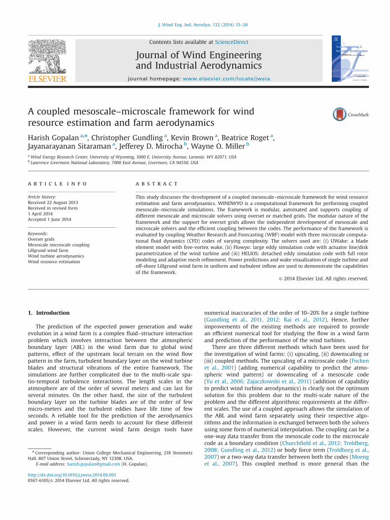
shown in Fig. 2(a)–(c). The outer box in Fig. 2 is a schematicrepresentation of the WRF domain while the inner shaded boxrepresents the CFD domain (referred as off-body domain). The off-body domain uses a single-block structured grid with grid refine-ment in the terrain normal direction, if required. The overset grid

boundaries at the interface between the off-body domain andWRFdomain are shown in Fig. 2(b) for a single grid line. It is notrequired to have only one line in the overset region. Multiple gridpoints can be used and the MMCI module takes care of calculationof the velocities and SGS quantities at all these locations. The WRFflow field information is interpolated to the off-body domain usingthe MMCI module while the turbulent viscosity in the CFD domainis calculated using Eq. (6). The interpolation information at theoverset grid boundaries are calculated dynamically to avoid sig-nificant overhead associated with storage of the WRF data in thememory for the entire time span. This setup is sufficient forperforming wind resource estimation studies. It should be notedthat for complex terrains, curvilinear single-block structured gridsare used and the MMCI module can account for the curvature inthe terrain. Fluid Structure Interaction capability can also be addedby incorporating the structural module to the microscale solver(Masarati and Sitaraman, 2011).

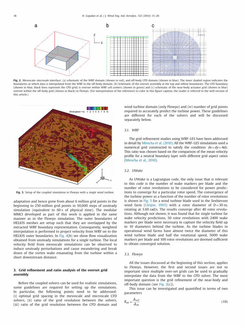
For modeling a wind turbine using actuator disc or actuatorline, cylindrical structured grids (referred as near-body domain)are overset inside the off-body domain. One such grid is used foreach turbine. This automates the grid generation process andmakes it easier to add any number of turbines in the CFD domainin a straight forward way without the need for multiple levels ofgrid refinement (Churchfield et al., 2012). When finer grids arerequired in the region near the wind turbine, an additional bufferdomain is overset between the outer off-body domain and thenear-body domain. This avoids a significant jump in the gridresolution ratios, albeit with increase in the computational time.The overlapping regions of the off-body and near-body grids areshown in Fig. 2(c) for a single turbine grid. Once the grids for allthe wind turbines have been assembled, the WRF flow fieldinformation is used to initialize both the domains. In this way,the simulations can be started using realistic initial conditions. Thesimulations are performed after the initial conditions have beengenerated. A sample flow field for a coupled simulation with asingle wind turbine is shown in Fig. 3. It should be noted that thetime step of simulation in Flowyo is much smaller than the WRFsimulations. A weighted linear interpolation is used for interpola-tion of boundary data from WRF to the CFD domain at time stepswhich do not coincide with the WRF data.

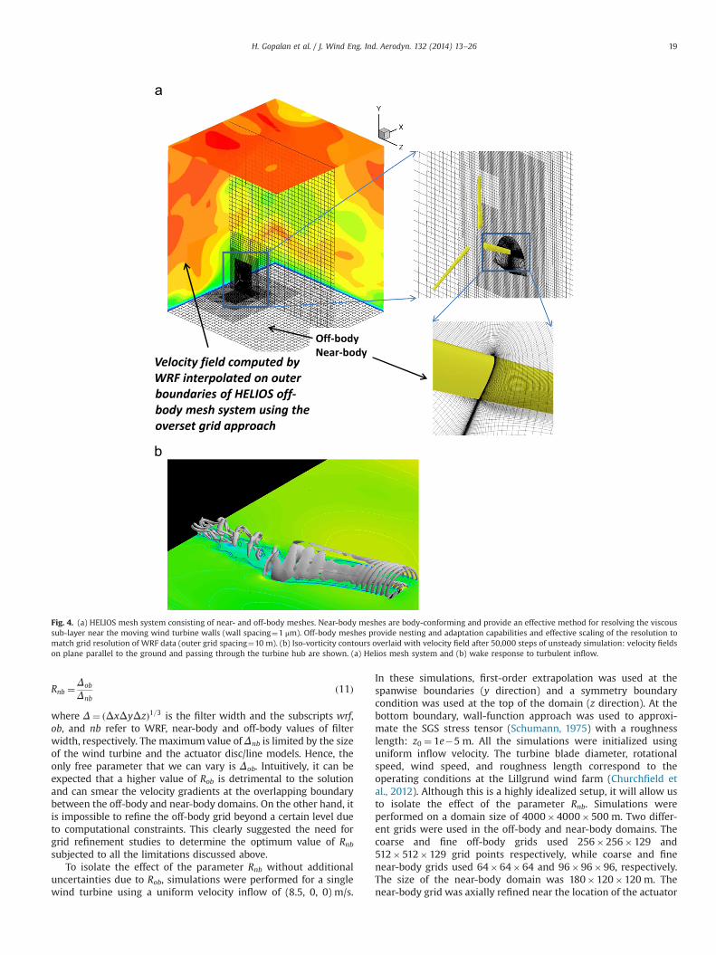
2.4.3. HELIOSHELIOS mesh system consists of body conforming (termed

near-body meshes) that are overlapped by a system of nestedCartesian grids of incremental resolution. A sample grid from atypical HELIOS detached eddy simulation is shown in Fig. 4(a).Near-body meshes that conform to this three bladed turbineconsisted of 2.15 million grid points with stretched cells at thesurface to provide enough resolution to match the viscous sub-layer requirement for near-body RANS simulations ðyþ r1Þ. Theoff-body grid LES system is capable of dynamic feature based

Fig. 1. Instantaneous wind speed along a spanwise plane to demonstrate the synthetic small-scale model: (a) no added fluctuations and (b) fluctuations added using thesmall-scale model.

H. Gopalan et al. / J. Wind Eng. Ind. Aerodyn. 132 (2014) 13–26 17

adaptation and hence grew from about 6 million grid points in thebeginning to 250 million grid points in 50,000 steps of unsteadysimulation (equivalent to 60 s of physical time). The modularMMCI developed as part of this work is applied in the samemanner as in the Flowyo simulation. The outer boundaries ofHELIOS meshes are setup such that they are overlapped by theextracted WRF boundary representation. Consequently, weightedinterpolation is performed to project velocity from WRF on to theHELIOS outer boundaries. In Fig. 4(b) we show flow visualizationobtained from unsteady simulations for a single turbine. The localvelocity field from mesoscale simulations can be observed toinduce unsteady perturbations and cause meandering and breakdown of the vortex wake emanating from the turbine within ashort downstream distance.

3. Grid refinement and ratio analysis of the overset gridassembly

Before the coupled solvers can be used for realistic simulations,some guidelines are required for setting up the simulations.In particular, the following points need to be addressed:(i) optimal grid spacing in the mesoscale and microscale CFDsolvers, (ii) ratio of the grid resolution between the solvers,(iii) ratio of the grid resolution between the CFD domain and

wind turbine domain (only Flowyo) and (iv) number of grid pointsrequired to accurately predict the turbine power. These guidelinesare different for each of the solvers and will be discussedseparately below.

3.1. WRF

The grid refinement studies using WRF–LES have been addressedin detail by Mirocha et al. (2010). All the WRF–LES simulations used anumerical grid constructed to satisfy the condition: dx¼dy¼4dz.This ratio was chosen based on the comparison of the mean velocityprofile for a neutral boundary layer with different grid aspect ratios(Mirocha et al., 2010).

3.2. UWake

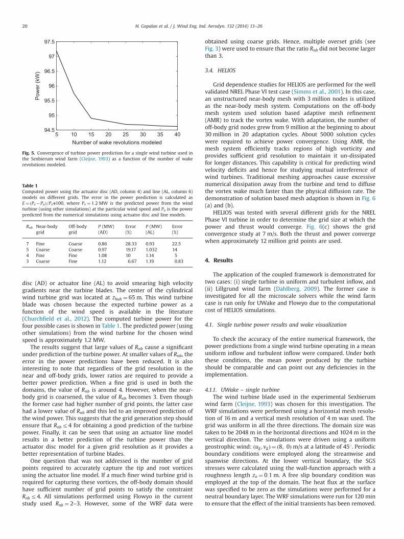
As UWake is a Lagrangian code, the only issue that is relevantto this code is the number of wake markers per blade and thenumber of rotor revolutions to be considered for power predic-tions to converge for a particular rotor speed. The convergence ofthe turbine power as a function of the number of rotor revolutionsis shown in Fig. 5 for a wind turbine blade used in the Sexbierumwind farm (Cleijne, 1993) with a rotor diameter of D¼30 m,rotating at 3.69 rad/s. The results converge after 40 rotor revolu-tions. Although not shown, it was found that for single turbine farwake velocity predictions, 50 rotor revolutions with 2400 wakemarkers per blade were necessary to capture the velocity field upto 10 diameters behind the turbine. As the turbine blades inoperational wind farms have almost twice the diameter of thiswind turbine blade and half the rotational speed, 5000 wakemarkers per blade and 100 rotor revolutions are deemed sufficientto obtain converged solution.

3.3. Flowyo

All the issues discussed at the beginning of this section, appliesto Flowyo. However, the first and second issues are not soimportant since multiple over-set grids can be used to graduallyinterpolate the data from the WRF to the CFD solver. The mostimportant question is the grid refinement of the near-body andoff-body domain (see Fig. 2(c)).

This issue can be investigated and quantified in terms of twoparameters

Rob ¼Δwrf

Δobð10Þ

Fig. 2. Mesoscale–microsale interface: (a) schematic of the WRF domain (shown in red), and off-body CFD domain (shown in blue). The inner shaded region indicates theboundaries at which data is interpolated from the WRF to the off-body domain. (b) Schematic of the overset assembly at the top and inflow boundaries. The CFD boundary(shown in blue, black lines represent the CFD grid) is overset within WRF cell centers (shown in green) and (c) schematic of the near-body actuator grid (shown in blue)overset within the off-body grid (shown in black) in Flowyo. (For interpretation of the references to color in this figure caption, the reader is referred to the web version ofthis article.)

Fig. 3. Setup of the coupled simulation in Flowyo with a single wind turbine.

H. Gopalan et al. / J. Wind Eng. Ind. Aerodyn. 132 (2014) 13–2618

Rnb ¼Δob

Δnbð11Þ

where Δ¼ ðΔxΔyΔzÞ1=3 is the filter width and the subscripts wrf,ob, and nb refer to WRF, near-body and off-body values of filterwidth, respectively. The maximum value of Δnb is limited by the sizeof the wind turbine and the actuator disc/line models. Hence, theonly free parameter that we can vary is Δob. Intuitively, it can beexpected that a higher value of Rob is detrimental to the solutionand can smear the velocity gradients at the overlapping boundarybetween the off-body and near-body domains. On the other hand, itis impossible to refine the off-body grid beyond a certain level dueto computational constraints. This clearly suggested the need forgrid refinement studies to determine the optimum value of Rnbsubjected to all the limitations discussed above.

To isolate the effect of the parameter Rnb without additionaluncertainties due to Rob, simulations were performed for a singlewind turbine using a uniform velocity inflow of (8.5, 0, 0) m/s.

In these simulations, first-order extrapolation was used at thespanwise boundaries (y direction) and a symmetry boundarycondition was used at the top of the domain (z direction). At thebottom boundary, wall-function approach was used to approxi-mate the SGS stress tensor (Schumann, 1975) with a roughnesslength: z0 ¼ 1e�5 m. All the simulations were initialized usinguniform inflow velocity. The turbine blade diameter, rotationalspeed, wind speed, and roughness length correspond to theoperating conditions at the Lillgrund wind farm (Churchfield etal., 2012). Although this is a highly idealized setup, it will allow usto isolate the effect of the parameter Rnb. Simulations wereperformed on a domain size of 4000�4000�500 m. Two differ-ent grids were used in the off-body and near-body domains. Thecoarse and fine off-body grids used 256�256�129 and512�512�129 grid points respectively, while coarse and finenear-body grids used 64�64�64 and 96�96�96, respectively.The size of the near-body domain was 180�120�120 m. Thenear-body grid was axially refined near the location of the actuator

Fig. 4. (a) HELIOS mesh system consisting of near- and off-body meshes. Near-body meshes are body-conforming and provide an effective method for resolving the viscoussub-layer near the moving wind turbine walls (wall spacing¼1 μm). Off-body meshes provide nesting and adaptation capabilities and effective scaling of the resolution tomatch grid resolution of WRF data (outer grid spacing¼10 m). (b) Iso-vorticity contours overlaid with velocity field after 50,000 steps of unsteady simulation: velocity fieldson plane parallel to the ground and passing through the turbine hub are shown. (a) Helios mesh system and (b) wake response to turbulent inflow.

H. Gopalan et al. / J. Wind Eng. Ind. Aerodyn. 132 (2014) 13–26 19

disc (AD) or actuator line (AL) to avoid smearing high velocitygradients near the turbine blades. The center of the cylindricalwind turbine grid was located at zhub ¼ 65 m. This wind turbineblade was chosen because the expected turbine power as afunction of the wind speed is available in the literature(Churchfield et al., 2012). The computed turbine power for thefour possible cases is shown in Table 1. The predicted power (usingother simulations) from the wind turbine for the chosen windspeed is approximately 1.2 MW.

The results suggest that large values of Rnb cause a significantunder prediction of the turbine power. At smaller values of Rnb, theerror in the power predictions have been reduced. It is alsointeresting to note that regardless of the grid resolution in thenear and off-body grids, lower ratios are required to provide abetter power prediction. When a fine grid is used in both thedomains, the value of Rnb is around 4. However, when the near-body grid is coarsened, the value of Rnb becomes 3. Even thoughthe former case had higher number of grid points, the latter casehad a lower value of Rnb and this led to an improved prediction ofthe wind power. This suggests that the grid generation step shouldensure that Rnbr4 for obtaining a good prediction of the turbinepower. Finally, it can be seen that using an actuator line modelresults in a better prediction of the turbine power than theactuator disc model for a given grid resolution as it provides abetter representation of turbine blades.

One question that was not addressed is the number of gridpoints required to accurately capture the tip and root vorticesusing the actuator line model. If a much finer wind turbine grid isrequired for capturing these vortices, the off-body domain shouldhave sufficient number of grid points to satisfy the constraintRnbr4. All simulations performed using Flowyo in the currentstudy used Rnb ¼ 2–3. However, some of the WRF data were

obtained using coarse grids. Hence, multiple overset grids (seeFig. 3) were used to ensure that the ratio Rnb did not become largerthan 3.

3.4. HELIOS

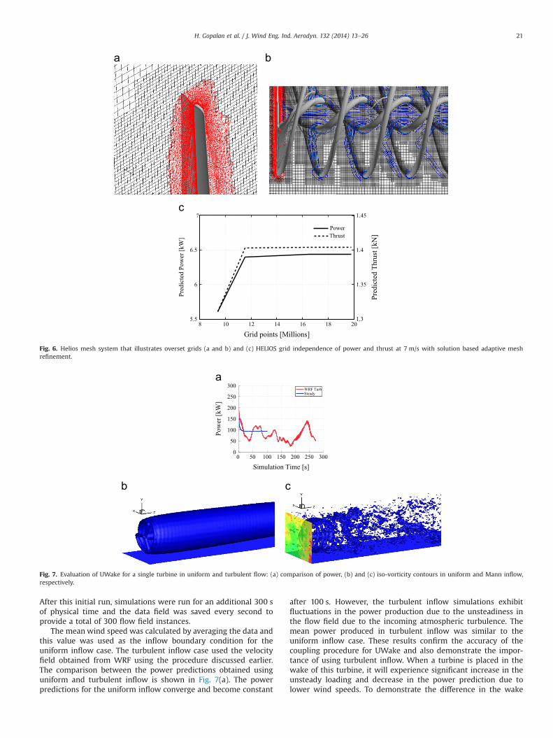
Grid dependence studies for HELIOS are performed for the wellvalidated NREL Phase VI test case (Simms et al., 2001). In this case,an unstructured near-body mesh with 3 million nodes is utilizedas the near-body mesh system. Computations on the off-bodymesh system used solution based adaptive mesh refinement(AMR) to track the vortex wake. With adaptation, the number ofoff-body grid nodes grew from 9 million at the beginning to about30 million in 20 adaptation cycles. About 5000 solution cycleswere required to achieve power convergence. Using AMR, themesh system efficiently tracks regions of high vorticity andprovides sufficient grid resolution to maintain it un-dissipatedfor longer distances. This capability is critical for predicting windvelocity deficits and hence for studying mutual interference ofwind turbines. Traditional meshing approaches cause excessivenumerical dissipation away from the turbine and tend to diffusethe vortex wake much faster than the physical diffusion rate. Thedemonstration of solution based mesh adaption is shown in Fig. 6(a) and (b).

HELIOS was tested with several different grids for the NRELPhase VI turbine in order to determine the grid size at which thepower and thrust would converge. Fig. 6(c) shows the gridconvergence study at 7 m/s. Both the thrust and power convergewhen approximately 12 million grid points are used.

4. Results

The application of the coupled framework is demonstrated fortwo cases: (i) single turbine in uniform and turbulent inflow, and(ii) Lillgrund wind farm (Dahlberg, 2009). The former case isinvestigated for all the microscale solvers while the wind farmcase is run only for UWake and Flowyo due to the computationalcost of HELIOS simulations.

4.1. Single turbine power results and wake visualization

To check the accuracy of the entire numerical framework, thepower predictions from a single wind turbine operating in a meanuniform inflow and turbulent inflow were compared. Under boththese conditions, the mean power produced by the turbineshould be comparable and can point out any deficiencies in theimplementation.

4.1.1. UWake – single turbineThe wind turbine blade used in the experimental Sexbierum

wind farm (Cleijne, 1993) was chosen for this investigation. TheWRF simulations were performed using a horizontal mesh resolu-tion of 16 m and a vertical mesh resolution of 4 m was used. Thegrid was uniform in all the three directions. The domain size wastaken to be 2048 m in the horizontal directions and 1024 m in thevertical direction. The simulations were driven using a uniformgeostrophic wind: ðug ; vgÞ ¼ ð8; 0Þm/s at a latitude of 451. Periodicboundary conditions were employed along the streamwise andspanwise directions. At the lower vertical boundary, the SGSstresses were calculated using the wall-function approach with aroughness length zo ¼ 0:1 m. A free slip boundary condition wasemployed at the top of the domain. The heat flux at the surfacewas specified to be zero as the simulations were performed for aneutral boundary layer. The WRF simulations were run for 120 minto ensure that the effect of the initial transients has been removed.

Table 1Computed power using the actuator disc (AD, column 4) and line (AL, column 6)models on different grids. The error in the power prediction is calculated asE¼ ðPe�PaÞ=Pen100, where Pe ¼ 1:2 MW is the predicted power from the windturbine (using other simulations) at the particular wind speed and Pa is the powerpredicted from the numerical simulations using actuator disc and line models.

Rnb Near-bodygrid

Off-bodygrid

P (MW)(AD)

Error(%)

P (MW)(AL)

Error(%)

7 Fine Coarse 0.86 28.33 0.93 22.55 Coarse Coarse 0.97 19.17 1.032 144 Fine Fine 1.08 10 1.14 53 Coarse Fine 1.12 6.67 1.19 0.83

94.5

95

95.5

96

96.5

97

97.5

5 10 15 20 25 30 35 40

Pow

er (k

W)

Number of wake revolutions modeled

Fig. 5. Convergence of turbine power prediction for a single wind turbine used inthe Sexbierum wind farm (Cleijne, 1993) as a function of the number of wakerevolutions modeled.

H. Gopalan et al. / J. Wind Eng. Ind. Aerodyn. 132 (2014) 13–2620

After this initial run, simulations were run for an additional 300 sof physical time and the data field was saved every second toprovide a total of 300 flow field instances.

The mean wind speed was calculated by averaging the data andthis value was used as the inflow boundary condition for theuniform inflow case. The turbulent inflow case used the velocityfield obtained from WRF using the procedure discussed earlier.The comparison between the power predictions obtained usinguniform and turbulent inflow is shown in Fig. 7(a). The powerpredictions for the uniform inflow converge and become constant

after 100 s. However, the turbulent inflow simulations exhibitfluctuations in the power production due to the unsteadiness inthe flow field due to the incoming atmospheric turbulence. Themean power produced in turbulent inflow was similar to theuniform inflow case. These results confirm the accuracy of thecoupling procedure for UWake and also demonstrate the impor-tance of using turbulent inflow. When a turbine is placed in thewake of this turbine, it will experience significant increase in theunsteady loading and decrease in the power prediction due tolower wind speeds. To demonstrate the difference in the wake

8 10 12 14 16 18 205.5

6

6.5

7

Grid points [Millions]

Pred

icte

d Po

wer

[kW

]

1.3

1.35

1.4

1.45

Pred

icte

d Th

rust

[kN

]

PowerThrust

Fig. 6. Helios mesh system that illustrates overset grids (a and b) and (c) HELIOS grid independence of power and thrust at 7 m/s with solution based adaptive meshrefinement.

0 50 100 150 200 250 3000

50

100

150

200

250

300

Simulation Time [s]

Pow

er [k

W]

WRF TurbSteady

Fig. 7. Evaluation of UWake for a single turbine in uniform and turbulent flow: (a) comparison of power, (b) and (c) iso-vorticity contours in uniform and Mann inflow,respectively.

H. Gopalan et al. / J. Wind Eng. Ind. Aerodyn. 132 (2014) 13–26 21

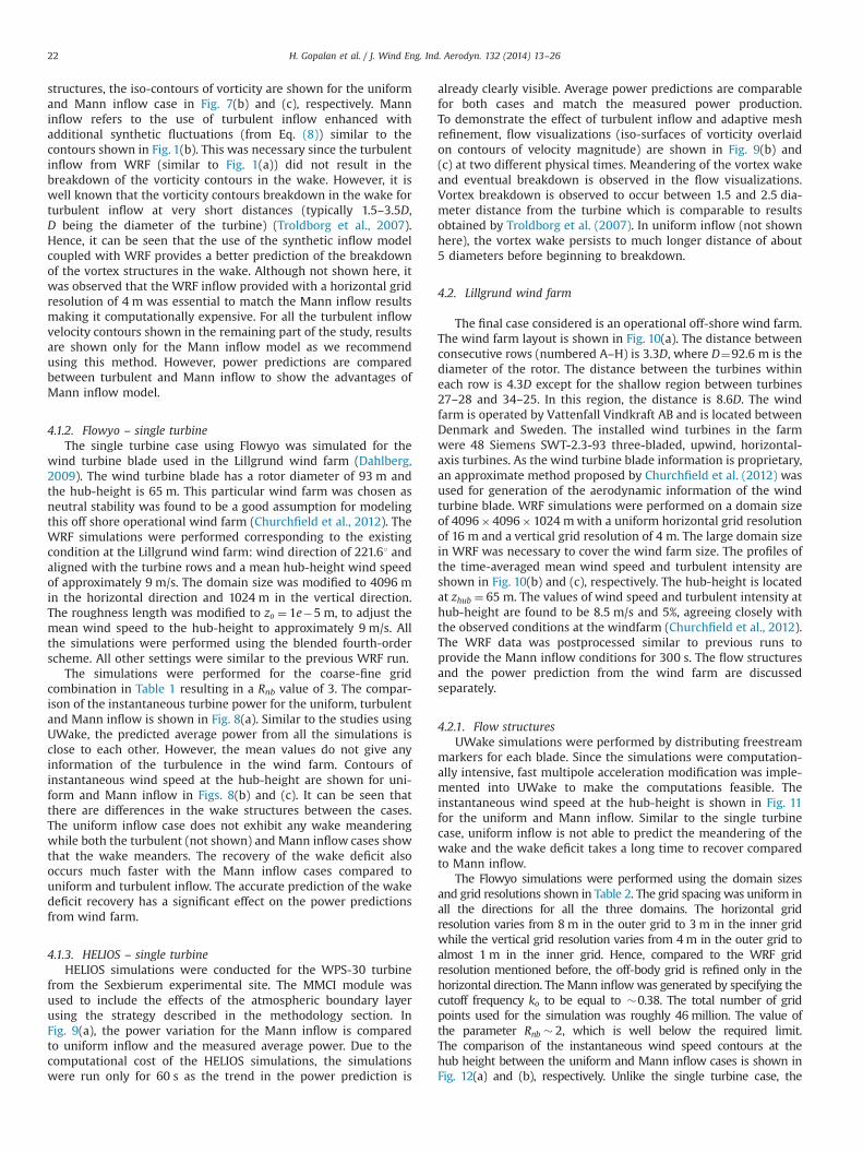
structures, the iso-contours of vorticity are shown for the uniformand Mann inflow case in Fig. 7(b) and (c), respectively. Manninflow refers to the use of turbulent inflow enhanced withadditional synthetic fluctuations (from Eq. (8)) similar to thecontours shown in Fig. 1(b). This was necessary since the turbulentinflow from WRF (similar to Fig. 1(a)) did not result in thebreakdown of the vorticity contours in the wake. However, it iswell known that the vorticity contours breakdown in the wake forturbulent inflow at very short distances (typically 1.5–3.5D,D being the diameter of the turbine) (Troldborg et al., 2007).Hence, it can be seen that the use of the synthetic inflow modelcoupled with WRF provides a better prediction of the breakdownof the vortex structures in the wake. Although not shown here, itwas observed that the WRF inflow provided with a horizontal gridresolution of 4 m was essential to match the Mann inflow resultsmaking it computationally expensive. For all the turbulent inflowvelocity contours shown in the remaining part of the study, resultsare shown only for the Mann inflow model as we recommendusing this method. However, power predictions are comparedbetween turbulent and Mann inflow to show the advantages ofMann inflow model.

4.1.2. Flowyo – single turbineThe single turbine case using Flowyo was simulated for the

wind turbine blade used in the Lillgrund wind farm (Dahlberg,2009). The wind turbine blade has a rotor diameter of 93 m andthe hub-height is 65 m. This particular wind farm was chosen asneutral stability was found to be a good assumption for modelingthis off shore operational wind farm (Churchfield et al., 2012). TheWRF simulations were performed corresponding to the existingcondition at the Lillgrund wind farm: wind direction of 221.61 andaligned with the turbine rows and a mean hub-height wind speedof approximately 9 m/s. The domain size was modified to 4096 min the horizontal direction and 1024 m in the vertical direction.The roughness length was modified to zo ¼ 1e�5 m, to adjust themean wind speed to the hub-height to approximately 9 m/s. Allthe simulations were performed using the blended fourth-orderscheme. All other settings were similar to the previous WRF run.

The simulations were performed for the coarse-fine gridcombination in Table 1 resulting in a Rnb value of 3. The compar-ison of the instantaneous turbine power for the uniform, turbulentand Mann inflow is shown in Fig. 8(a). Similar to the studies usingUWake, the predicted average power from all the simulations isclose to each other. However, the mean values do not give anyinformation of the turbulence in the wind farm. Contours ofinstantaneous wind speed at the hub-height are shown for uni-form and Mann inflow in Figs. 8(b) and (c). It can be seen thatthere are differences in the wake structures between the cases.The uniform inflow case does not exhibit any wake meanderingwhile both the turbulent (not shown) and Mann inflow cases showthat the wake meanders. The recovery of the wake deficit alsooccurs much faster with the Mann inflow cases compared touniform and turbulent inflow. The accurate prediction of the wakedeficit recovery has a significant effect on the power predictionsfrom wind farm.

4.1.3. HELIOS – single turbineHELIOS simulations were conducted for the WPS-30 turbine

from the Sexbierum experimental site. The MMCI module wasused to include the effects of the atmospheric boundary layerusing the strategy described in the methodology section. InFig. 9(a), the power variation for the Mann inflow is comparedto uniform inflow and the measured average power. Due to thecomputational cost of the HELIOS simulations, the simulationswere run only for 60 s as the trend in the power prediction is

already clearly visible. Average power predictions are comparablefor both cases and match the measured power production.To demonstrate the effect of turbulent inflow and adaptive meshrefinement, flow visualizations (iso-surfaces of vorticity overlaidon contours of velocity magnitude) are shown in Fig. 9(b) and(c) at two different physical times. Meandering of the vortex wakeand eventual breakdown is observed in the flow visualizations.Vortex breakdown is observed to occur between 1.5 and 2.5 dia-meter distance from the turbine which is comparable to resultsobtained by Troldborg et al. (2007). In uniform inflow (not shownhere), the vortex wake persists to much longer distance of about5 diameters before beginning to breakdown.

4.2. Lillgrund wind farm

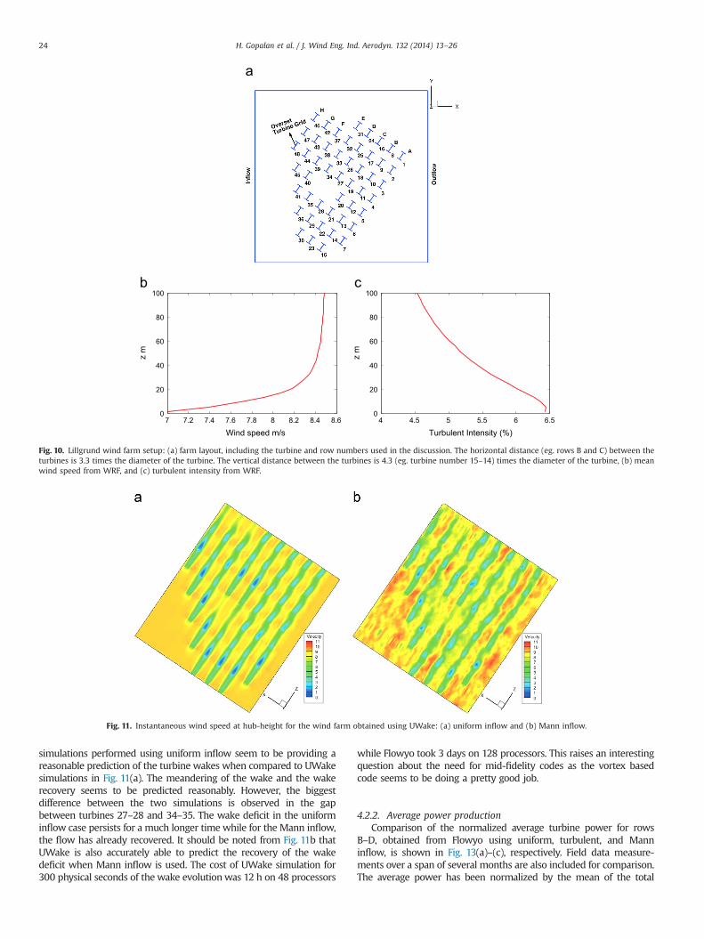
The final case considered is an operational off-shore wind farm.The wind farm layout is shown in Fig. 10(a). The distance betweenconsecutive rows (numbered A–H) is 3.3D, where D¼92.6 m is thediameter of the rotor. The distance between the turbines withineach row is 4.3D except for the shallow region between turbines27–28 and 34–25. In this region, the distance is 8.6D. The windfarm is operated by Vattenfall Vindkraft AB and is located betweenDenmark and Sweden. The installed wind turbines in the farmwere 48 Siemens SWT-2.3-93 three-bladed, upwind, horizontal-axis turbines. As the wind turbine blade information is proprietary,an approximate method proposed by Churchfield et al. (2012) wasused for generation of the aerodynamic information of the windturbine blade. WRF simulations were performed on a domain sizeof 4096�4096�1024 mwith a uniform horizontal grid resolutionof 16 m and a vertical grid resolution of 4 m. The large domain sizein WRF was necessary to cover the wind farm size. The profiles ofthe time-averaged mean wind speed and turbulent intensity areshown in Fig. 10(b) and (c), respectively. The hub-height is locatedat zhub ¼ 65 m. The values of wind speed and turbulent intensity athub-height are found to be 8.5 m/s and 5%, agreeing closely withthe observed conditions at the windfarm (Churchfield et al., 2012).The WRF data was postprocessed similar to previous runs toprovide the Mann inflow conditions for 300 s. The flow structuresand the power prediction from the wind farm are discussedseparately.

4.2.1. Flow structuresUWake simulations were performed by distributing freestream

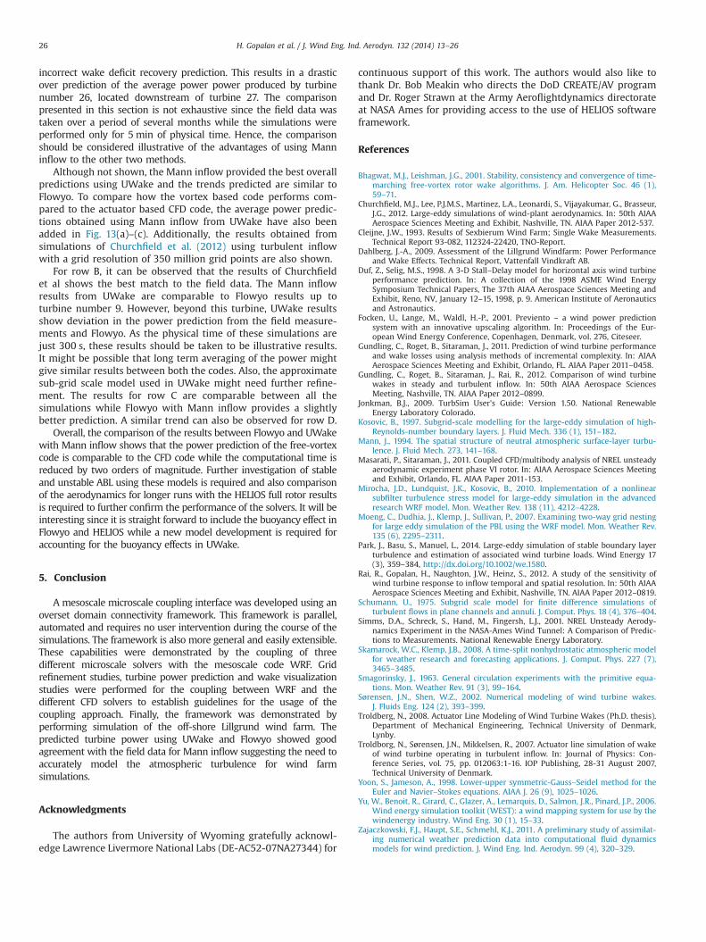
markers for each blade. Since the simulations were computation-ally intensive, fast multipole acceleration modification was imple-mented into UWake to make the computations feasible. Theinstantaneous wind speed at the hub-height is shown in Fig. 11for the uniform and Mann inflow. Similar to the single turbinecase, uniform inflow is not able to predict the meandering of thewake and the wake deficit takes a long time to recover comparedto Mann inflow.

The Flowyo simulations were performed using the domain sizesand grid resolutions shown in Table 2. The grid spacing was uniform inall the directions for all the three domains. The horizontal gridresolution varies from 8m in the outer grid to 3 m in the inner gridwhile the vertical grid resolution varies from 4m in the outer grid toalmost 1 m in the inner grid. Hence, compared to the WRF gridresolution mentioned before, the off-body grid is refined only in thehorizontal direction. The Mann inflowwas generated by specifying thecutoff frequency ko to be equal to �0.38. The total number of gridpoints used for the simulation was roughly 46 million. The value ofthe parameter Rnb � 2, which is well below the required limit.The comparison of the instantaneous wind speed contours at thehub height between the uniform and Mann inflow cases is shown inFig. 12(a) and (b), respectively. Unlike the single turbine case, the

H. Gopalan et al. / J. Wind Eng. Ind. Aerodyn. 132 (2014) 13–2622

600

800

1000

1200

1400

1600

1800

2000

2200

2400

0 5000 10000 15000 20000 25000 30000

Pow

er (k

W)

Time step

SteadyTurbulent

Turbulent - Mann

Fig. 8. Evaluation of Flowyo for a single turbine in uniform and turbulent flow: (a) comparison of power, (b) and (c) velocity contours in uniform and Mann inflow,respectively.

-100-50

0 50

100 150 200 250 300 350

0 5 10 15 20 25 30 35 40

Pow

er [k

W]

time [seconds]

WRF/HeliosHelios (8 m/s)

Measured (8 m/s)

Fig. 9. Evaluation of Flowyo for a single turbine in uniform and turbulent flow: (a) comparison of power, (b) and (c) iso surfaces of vorticity (ω¼0.003) overlaid with velocitycontours for turbulent inflow at different physical times. Grid systems are also overlaid on the flow visualizations to show the efficacy of solution based AMR: (b) t¼11 s and(c) t¼59 s.

H. Gopalan et al. / J. Wind Eng. Ind. Aerodyn. 132 (2014) 13–26 23

simulations performed using uniform inflow seem to be providing areasonable prediction of the turbine wakes when compared to UWakesimulations in Fig. 11(a). The meandering of the wake and the wakerecovery seems to be predicted reasonably. However, the biggestdifference between the two simulations is observed in the gapbetween turbines 27–28 and 34–35. The wake deficit in the uniforminflow case persists for a much longer time while for the Mann inflow,the flow has already recovered. It should be noted from Fig. 11b thatUWake is also accurately able to predict the recovery of the wakedeficit when Mann inflow is used. The cost of UWake simulation for300 physical seconds of the wake evolutionwas 12 h on 48 processors

while Flowyo took 3 days on 128 processors. This raises an interestingquestion about the need for mid-fidelity codes as the vortex basedcode seems to be doing a pretty good job.

4.2.2. Average power productionComparison of the normalized average turbine power for rows

B–D, obtained from Flowyo using uniform, turbulent, and Manninflow, is shown in Fig. 13(a)–(c), respectively. Field data measure-ments over a span of several months are also included for comparison.The average power has been normalized by the mean of the total

0

20

40

60

80

100

7 7.2 7.4 7.6 7.8 8 8.2 8.4 8.6

z m

Wind speed m/s

0

20

40

60

80

100

4 4.5 5 5.5 6 6.5

z m

Turbulent Intensity (%)

Fig. 10. Lillgrund wind farm setup: (a) farm layout, including the turbine and row numbers used in the discussion. The horizontal distance (eg. rows B and C) between theturbines is 3.3 times the diameter of the turbine. The vertical distance between the turbines is 4.3 (eg. turbine number 15–14) times the diameter of the turbine, (b) meanwind speed from WRF, and (c) turbulent intensity from WRF.

Fig. 11. Instantaneous wind speed at hub-height for the wind farm obtained using UWake: (a) uniform inflow and (b) Mann inflow.

H. Gopalan et al. / J. Wind Eng. Ind. Aerodyn. 132 (2014) 13–2624

power produced by the first turbine in each row. The results show thatthe most significant impact of the turbine wake is the significant dropin the power produced by the second turbine in the row. This effect is

also present up to the fifth turbine in rows B and C. Beyond theserows, there is a slight recovery of the turbine power loss. For turbinesin row D, there is an increase of the power production in the fourthturbine due to the additional spacing between turbines (shallowwaterregion). The fourth turbine recovers approximately 20% of additionalturbine power compared to the second and the third turbines. Forturbines located beyond the fourth turbine in row D, the drop in thepower production is comparable to the other rows.

The differences between the Mann, turbulent and uniform infloware clearly visible by comparing the turbine power production. Theuse of uniform inflow results in a significant under prediction of theaverage turbine power in rows B and C. In row D, uniform inflow caseclearly changes the physics between the turbine number 27 due to

Fig. 12. Instantaneous wind speed at hub-height for the wind farm obtained using Flowyo: (a) uniform inflow and (b) Mann inflow.

0.2

0.4

0.6

0.8

1

8 9 10 11 12 13 14 15

3P/(P

15+P

23+P

30)

Turbine Number

0.2

0.4

0.6

0.8

1

16 17 18 19 20 21 22 23

3P/(P

15+P

23+P

30)

Turbine Number

0.2

0.4

0.6

0.8

1

24 25 26 27 28 29 30

3P/(P

15+P

23+P

30)

Turbine Number

Uniform InflowTurbulent Inflow

Mann InflowUWake Mann Inflow

Churchfield Field Data

Fig. 13. Comparison of relative turbine power for rows B–D for the Lillgrund wind farm between uniform inflow, turbulent inflow, Mann inflow, field data and simulations ofChurchfield et al. (2012): (a) row B, (b) row C and (c) row D.

Table 2Domain sizes and grid spacing for the Lillgrund wind farm simulation usingFlowyo.

Grid Domain (m) Resolution

Off-body outer 3960�3960�240 490 �490�61Buffer 320�200�180 80�50�90Near-body 240�60�60 80�54�54

H. Gopalan et al. / J. Wind Eng. Ind. Aerodyn. 132 (2014) 13–26 25

incorrect wake deficit recovery prediction. This results in a drasticover prediction of the average power power produced by turbinenumber 26, located downstream of turbine 27. The comparisonpresented in this section is not exhaustive since the field data wastaken over a period of several months while the simulations wereperformed only for 5 min of physical time. Hence, the comparisonshould be considered illustrative of the advantages of using Manninflow to the other two methods.

Although not shown, the Mann inflow provided the best overallpredictions using UWake and the trends predicted are similar toFlowyo. To compare how the vortex based code performs com-pared to the actuator based CFD code, the average power predic-tions obtained using Mann inflow from UWake have also beenadded in Fig. 13(a)–(c). Additionally, the results obtained fromsimulations of Churchfield et al. (2012) using turbulent inflowwith a grid resolution of 350 million grid points are also shown.

For row B, it can be observed that the results of Churchfieldet al shows the best match to the field data. The Mann inflowresults from UWake are comparable to Flowyo results up toturbine number 9. However, beyond this turbine, UWake resultsshow deviation in the power prediction from the field measure-ments and Flowyo. As the physical time of these simulations arejust 300 s, these results should be taken to be illustrative results.It might be possible that long term averaging of the power mightgive similar results between both the codes. Also, the approximatesub-grid scale model used in UWake might need further refine-ment. The results for row C are comparable between all thesimulations while Flowyo with Mann inflow provides a slightlybetter prediction. A similar trend can also be observed for row D.

Overall, the comparison of the results between Flowyo and UWakewith Mann inflow shows that the power prediction of the free-vortexcode is comparable to the CFD code while the computational time isreduced by two orders of magnitude. Further investigation of stableand unstable ABL using these models is required and also comparisonof the aerodynamics for longer runs with the HELIOS full rotor resultsis required to further confirm the performance of the solvers. It will beinteresting since it is straight forward to include the buoyancy effect inFlowyo and HELIOS while a new model development is required foraccounting for the buoyancy effects in UWake.

5. Conclusion

A mesoscale microscale coupling interface was developed using anoverset domain connectivity framework. This framework is parallel,automated and requires no user intervention during the course of thesimulations. The framework is also more general and easily extensible.These capabilities were demonstrated by the coupling of threedifferent microscale solvers with the mesoscale code WRF. Gridrefinement studies, turbine power prediction and wake visualizationstudies were performed for the coupling between WRF and thedifferent CFD solvers to establish guidelines for the usage of thecoupling approach. Finally, the framework was demonstrated byperforming simulation of the off-shore Lillgrund wind farm. Thepredicted turbine power using UWake and Flowyo showed goodagreement with the field data for Mann inflow suggesting the need toaccurately model the atmospheric turbulence for wind farmsimulations.

Acknowledgments

The authors from University of Wyoming gratefully acknowl-edge Lawrence Livermore National Labs (DE-AC52-07NA27344) for

continuous support of this work. The authors would also like tothank Dr. Bob Meakin who directs the DoD CREATE/AV programand Dr. Roger Strawn at the Army Aeroflightdynamics directorateat NASA Ames for providing access to the use of HELIOS softwareframework.

References

Bhagwat, M.J., Leishman, J.G., 2001. Stability, consistency and convergence of time-marching free-vortex rotor wake algorithms. J. Am. Helicopter Soc. 46 (1),59–71.

Churchfield, M.J., Lee, P.J.M.S., Martinez, L.A., Leonardi, S., Vijayakumar, G., Brasseur,J.G., 2012. Large-eddy simulations of wind-plant aerodynamics. In: 50th AIAAAerospace Sciences Meeting and Exhibit, Nashville, TN. AIAA Paper 2012-537.

Cleijne, J.W., 1993. Results of Sexbierum Wind Farm; Single Wake Measurements.Technical Report 93-082, 112324-22420, TNO-Report.

Dahlberg, J.-A., 2009. Assessment of the Lillgrund Windfarm: Power Performanceand Wake Effects. Technical Report, Vattenfall Vindkraft AB.

Duf, Z., Selig, M.S., 1998. A 3-D Stall–Delay model for horizontal axis wind turbineperformance prediction. In: A collection of the 1998 ASME Wind EnergySymposium Technical Papers, The 37th AIAA Aerospace Sciences Meeting andExhibit, Reno, NV, January 12–15, 1998, p. 9. American Institute of Aeronauticsand Astronautics.

Focken, U., Lange, M., Waldl, H.-P., 2001. Previento – a wind power predictionsystem with an innovative upscaling algorithm. In: Proceedings of the Eur-opean Wind Energy Conference, Copenhagen, Denmark, vol. 276, Citeseer.

Gundling, C., Roget, B., Sitaraman, J., 2011. Prediction of wind turbine performanceand wake losses using analysis methods of incremental complexity. In: AIAAAerospace Sciences Meeting and Exhibit, Orlando, FL. AIAA Paper 2011–0458.

Gundling, C., Roget, B., Sitaraman, J., Rai, R., 2012. Comparison of wind turbinewakes in steady and turbulent inflow. In: 50th AIAA Aerospace SciencesMeeting, Nashville, TN. AIAA Paper 2012–0899.

Jonkman, B.J., 2009. TurbSim User's Guide: Version 1.50. National RenewableEnergy Laboratory Colorado.

Kosovic, B., 1997. Subgrid-scale modelling for the large-eddy simulation of high-Reynolds-number boundary layers. J. Fluid Mech. 336 (1), 151–182.

Mann, J., 1994. The spatial structure of neutral atmospheric surface-layer turbu-lence. J. Fluid Mech. 273, 141–168.

Masarati, P., Sitaraman, J., 2011. Coupled CFD/multibody analysis of NREL unsteadyaerodynamic experiment phase VI rotor. In: AIAA Aerospace Sciences Meetingand Exhibit, Orlando, FL. AIAA Paper 2011-153.

Mirocha, J.D., Lundquist, J.K., Kosovic, B., 2010. Implementation of a nonlinearsubfilter turbulence stress model for large-eddy simulation in the advancedresearch WRF model. Mon. Weather Rev. 138 (11), 4212–4228.

Moeng, C., Dudhia, J., Klemp, J., Sullivan, P., 2007. Examining two-way grid nestingfor large eddy simulation of the PBL using the WRF model. Mon. Weather Rev.135 (6), 2295–2311.

Park, J., Basu, S., Manuel, L., 2014. Large-eddy simulation of stable boundary layerturbulence and estimation of associated wind turbine loads. Wind Energy 17(3), 359–384, http://dx.doi.org/10.1002/we.1580.

Rai, R., Gopalan, H., Naughton, J.W., Heinz, S., 2012. A study of the sensitivity ofwind turbine response to inflow temporal and spatial resolution. In: 50th AIAAAerospace Sciences Meeting and Exhibit, Nashville, TN. AIAA Paper 2012–0819.

Schumann, U., 1975. Subgrid scale model for finite difference simulations ofturbulent flows in plane channels and annuli. J. Comput. Phys. 18 (4), 376–404.

Simms, D.A., Schreck, S., Hand, M., Fingersh, L.J., 2001. NREL Unsteady Aerody-namics Experiment in the NASA-Ames Wind Tunnel: A Comparison of Predic-tions to Measurements. National Renewable Energy Laboratory.

Skamarock, W.C., Klemp, J.B., 2008. A time-split nonhydrostatic atmospheric modelfor weather research and forecasting applications. J. Comput. Phys. 227 (7),3465–3485.

Smagorinsky, J., 1963. General circulation experiments with the primitive equa-tions. Mon. Weather Rev. 91 (3), 99–164.

Sørensen, J.N., Shen, W.Z., 2002. Numerical modeling of wind turbine wakes.J. Fluids Eng. 124 (2), 393–399.

Troldberg, N., 2008. Actuator Line Modeling of Wind Turbine Wakes (Ph.D. thesis).Department of Mechanical Engineering, Technical University of Denmark,Lynby.

Troldborg, N., Sørensen, J.N., Mikkelsen, R., 2007. Actuator line simulation of wakeof wind turbine operating in turbulent inflow. In: Journal of Physics: Con-ference Series, vol. 75, pp. 012063:1-16. IOP Publishing, 28-31 August 2007,Technical University of Denmark.

Yoon, S., Jameson, A., 1998. Lower-upper symmetric-Gauss–Seidel method for theEuler and Navier–Stokes equations. AIAA J. 26 (9), 1025–1026.

Yu, W., Benoit, R., Girard, C., Glazer, A., Lemarquis, D., Salmon, J.R., Pinard, J.P., 2006.Wind energy simulation toolkit (WEST): a wind mapping system for use by thewindenergy industry. Wind Eng. 30 (1), 15–33.

Zajaczkowski, F.J., Haupt, S.E., Schmehl, K.J., 2011. A preliminary study of assimilat-ing numerical weather prediction data into computational fluid dynamicsmodels for wind prediction. J. Wind Eng. Ind. Aerodyn. 99 (4), 320–329.

H. Gopalan et al. / J. Wind Eng. Ind. Aerodyn. 132 (2014) 13–2626