Microscale Modeling of Fluid Flow in PorousMedium Systems

byJames McClure

A dissertation submitted to the faculty of the University of North Carolina at ChapelHill in partial fulfillment of the requirements for the degree of Doctor of Philosophy inthe Environmental Sciences and Engineering.

Chapel Hill2011

Approved by:

Cass T. Miller, Advisor

William G. Gray, Reader

Matthew Farthing, Reader

David Adalsteinsson, Reader

Sorin Mitran, Reader

Jan Prins, Reader

ABSTRACTJAMES MCCLURE: Microscale Modeling of Fluid Flow in Porous

Medium Systems.(Under the direction of Cass T. Miller.)

Proper mathematical description of macroscopic porous medium flows is essential for

the study of a wide range of subsurface contamination scenarios. Existing mathematical

formulations, however, demonstrate inadequacies that preclude the accurate description

of many systems. Multi-scale models developed using thermodynamically constrained

averaging theory (TCAT) rigorously define macroscopic variables in terms of more

well-understood microscopic counterparts, permitting detailed analysis of macroscopic

model forms based on microscale simulation and experiment. Within this framework,

the primary objectives of microscale modeling are to elucidate important physical mech-

anisms and to inform both the form of macroscale closure relations as well as associated

parameter values. In order to meet these goals, numerical tools must include: (1) sim-

ulations that provide accurate microscopic solutions for physical phenomena in large,

complex domains; (2) morphological analysis tools that can be used to upscale sim-

ulation results to larger scales as dictated by the associated theoretical framework.

Development of a numerical toolbox for microscale porous medium studies is consid-

ered in line with these objectives, including both implementation and optimization

strategies. High-performance implementations of the lattice Boltzmann method are

developed to simulate one- and two-phase flows using several computing platforms. A

modified marching cubes algorithm is developed to explicitly construct all entities in a

two-phase system, including all interfaces between the fluid and solid phases in addi-

tion to the three phase contact curve. These entities serve as a numerical skeleton for

upscaling multiphase porous medium simulation results to the macroscale. Based on

these tools, development of macroscopic constitutive laws is illustrated for a special case

of anisotropic flow in porous media. In this example, microscale simulation is used to

demonstrate a limitation of existing macroscopic forms for cases in which the momen-

tum resistance depends on the flow direction in addition to the orientation. A modified

macroscopic form is proposed in order to properly account for this phenomenon.

ii

TABLE OF CONTENTS

LIST OF TABLES . . . . . . . . . . . . . . . . . . . . . . . . . . . . . . . . . . vi

LIST OF FIGURES . . . . . . . . . . . . . . . . . . . . . . . . . . . . . . . . . vii

1 Introduction . . . . . . . . . . . . . . . . . . . . . . . . . . . . . . . . . . . 1

1.1 Flow and Transport in Porous Media: Scope and Significance . . . . . . 1

1.2 Scale Considerations . . . . . . . . . . . . . . . . . . . . . . . . . . . . 2

1.2.1 Scales of Interest for Porous Media . . . . . . . . . . . . . . . . 3

1.2.2 Microscale Simulation and Macroscale Model Development . . . 4

1.2.3 Sources of Microscale Information . . . . . . . . . . . . . . . . . 5

1.3 Macroscopic Modeling Approaches for Porous Media . . . . . . . . . . 7

1.3.1 Thermodynamically Constrained Averaging Theory . . . . . . . 9

1.4 Research Objectives . . . . . . . . . . . . . . . . . . . . . . . . . . . . 11

2 High Performance Implementations of the Lattice Boltzmann

Method . . . . . . . . . . . . . . . . . . . . . . . . . . . . . . . . . . . . . 12

2.1 Introduction . . . . . . . . . . . . . . . . . . . . . . . . . . . . . . . . . 12

2.2 Methods . . . . . . . . . . . . . . . . . . . . . . . . . . . . . . . . . . . 14

2.2.1 Model Problems for Porous Media . . . . . . . . . . . . . . . . . 14

2.2.2 Permeability Measurement . . . . . . . . . . . . . . . . . . . . . 14

2.2.3 Capillary Pressure - Saturation Relationships . . . . . . . . . . 15

iii

2.2.4 LBM Fundamentals . . . . . . . . . . . . . . . . . . . . . . . . . 16

2.2.5 Single-Component Multi-Relaxation Time Model . . . . . . . . 18

2.2.6 Multi-Component Shan-Chen MRT Model . . . . . . . . . . . . 20

2.3 Implementation and Optimization Approaches . . . . . . . . . . . . . . 21

2.3.1 Hardware Overview . . . . . . . . . . . . . . . . . . . . . . . . . 22

2.3.2 Serial CPU Implementations (C++) . . . . . . . . . . . . . . . 26

2.3.3 Parallel Implementation of the LBM (C++/MPI) . . . . . . . . 28

2.3.4 Node-level Implementation of the LBM . . . . . . . . . . . . . . 31

2.3.5 GPU Implementation of the LBM (CUDA) . . . . . . . . . . . . 31

2.4 Results . . . . . . . . . . . . . . . . . . . . . . . . . . . . . . . . . . . . 35

2.4.1 Serial CPU Implementation . . . . . . . . . . . . . . . . . . . . 35

2.4.2 MPI Implementation . . . . . . . . . . . . . . . . . . . . . . . . 38

2.4.3 GPU implementation . . . . . . . . . . . . . . . . . . . . . . . . 41

2.4.4 Model Problems for Porous Media . . . . . . . . . . . . . . . . . 42

2.5 Discussion . . . . . . . . . . . . . . . . . . . . . . . . . . . . . . . . . . 47

2.6 Conclusions . . . . . . . . . . . . . . . . . . . . . . . . . . . . . . . . . 49

3 Morphological Tools . . . . . . . . . . . . . . . . . . . . . . . . . . . . . . 51

3.1 Approximation of Interfacial Properties in Multiphase

Porous Medium Systems . . . . . . . . . . . . . . . . . . . . . . . . . . 51

3.1.1 Introduction . . . . . . . . . . . . . . . . . . . . . . . . . . . . . 51

3.2 Methods . . . . . . . . . . . . . . . . . . . . . . . . . . . . . . . . . . . 53

3.2.1 Marching cubes algorithm . . . . . . . . . . . . . . . . . . . . . 54

3.2.2 Porous media marching cubes approach . . . . . . . . . . . . . . 56

iv

3.2.3 Higher order porous media marching cubes approach . . . . . . 60

3.2.4 Approximation of mean curvatures . . . . . . . . . . . . . . . . 62

3.2.5 Data source . . . . . . . . . . . . . . . . . . . . . . . . . . . . . 64

3.3 Results . . . . . . . . . . . . . . . . . . . . . . . . . . . . . . . . . . . . 66

3.4 Discussion . . . . . . . . . . . . . . . . . . . . . . . . . . . . . . . . . . 72

3.5 Conclusions . . . . . . . . . . . . . . . . . . . . . . . . . . . . . . . . . 74

3.6 Additional Morphological Properties . . . . . . . . . . . . . . . . . . . 75

3.6.1 Contact Angle . . . . . . . . . . . . . . . . . . . . . . . . . . . . 75

3.7 Collective Rearrangement Sphere Packing Algorithm . . . . . . . . . . 77

4 Direction-Dependent Flow in Porous Media . . . . . . . . . . . . . . . . . 79

4.1 Introduction . . . . . . . . . . . . . . . . . . . . . . . . . . . . . . . . . 79

4.2 Background . . . . . . . . . . . . . . . . . . . . . . . . . . . . . . . . . 81

4.3 Methods . . . . . . . . . . . . . . . . . . . . . . . . . . . . . . . . . . . 85

4.3.1 Lattice Boltzmann Model . . . . . . . . . . . . . . . . . . . . . 85

4.3.2 Solid Geometry . . . . . . . . . . . . . . . . . . . . . . . . . . . 86

4.3.3 Anti-symmetric Orientation Tensor . . . . . . . . . . . . . . . . 87

4.4 Results . . . . . . . . . . . . . . . . . . . . . . . . . . . . . . . . . . . . 91

4.5 Conclusions . . . . . . . . . . . . . . . . . . . . . . . . . . . . . . . . . 95

5 Summary and Recommendations . . . . . . . . . . . . . . . . . . . . . . . 97

5.1 Single Phase Flow . . . . . . . . . . . . . . . . . . . . . . . . . . . . . . 98

5.2 Multiphase Flow . . . . . . . . . . . . . . . . . . . . . . . . . . . . . . 98

BIBLIOGRAPHY . . . . . . . . . . . . . . . . . . . . . . . . . . . . . . . . . . 101

v

LIST OF TABLES

2.1 Reported peak performance based on serial execution of

the D3Q19 BGK LBM for a variety of processors [183,

117, 116, 77]. . . . . . . . . . . . . . . . . . . . . . . . . . . . . . . . . 36

2.2 Basic computational and memory reference parameters

per lattice site for the LBM models considered in this work. . . . . . . 36

2.3 Overview of hardware specifications and LBM perfor-

mance for the parallel systems used in this work. . . . . . . . . . . . . . 38

3.1 Sets needed for the PMMC algorithm. . . . . . . . . . . . . . . . . . . 57

4.1 Properties for asymmetric porous media constituted of

solid grains defined by Eq. (4.28) . . . . . . . . . . . . . . . . . . . . . 94

vi

LIST OF FIGURES

1.1 Flow chart depicting a multi-scale modeling framework

for porous media . . . . . . . . . . . . . . . . . . . . . . . . . . . . . . 10

2.1 Random close-packing of 128,000 identical spheres in a

cubic domain. . . . . . . . . . . . . . . . . . . . . . . . . . . . . . . . . 15

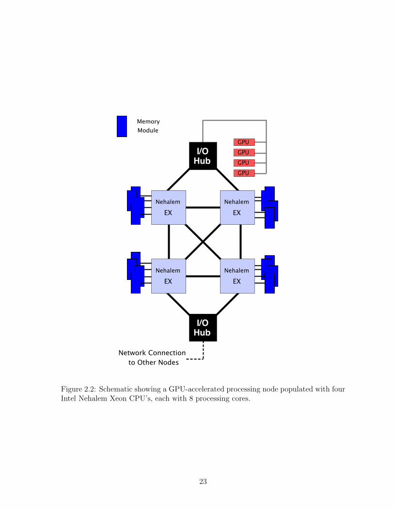
2.2 Schematic showing a GPU-accelerated processing node

populated with four Intel Nehalem Xeon CPU’s, each

with 8 processing cores. . . . . . . . . . . . . . . . . . . . . . . . . . . . 23

2.3 Typical GPU setup in which the CPU and GPU are uti-

lized in tandem. . . . . . . . . . . . . . . . . . . . . . . . . . . . . . . . 25

2.4 Domain structure for serial CPU implementation of the

LBM. Regular storage and access patterns are preserved

by storing ghost nodes for a halo of lattice sites on the

domain exterior and for sites within the solid phase (de-

noted by shaded gray circles). Interior and exterior lat-

tice sites are identified from index lists, which are used

to direct computations. . . . . . . . . . . . . . . . . . . . . . . . . . . . 27

2.5 Swap algorithm illustrated for the D2Q9 model: Non-

stationary distributions at a lattice site are swapped based

on the symmetry of the discrete velocity set. Note that

the D3Q19 velocity structure is identical to the D2Q9

structure in each coordinate plane. . . . . . . . . . . . . . . . . . . . . 27

2.6 Schematic summarizing communication between proces-

sors p and r in a parallel LB simulation using MPI. Dis-

tributions needed by processor r are packed into a send

buffer on processor p. Using MPI, these values are pro-

vided to a receive buffer on processor r, from which they

are unpacked to the proper location. . . . . . . . . . . . . . . . . . . . 29

vii

2.7 Domain decomposition for GPU implementation of the

LBM. In this 2-D analog, the 11 × 11 spatial domain is

divided into grid blocks (nBlocks = 4) with a fixed num-

ber of threads per threadblock (nThreads = 8). With

nBlocks and nThreads fixed, each thread performs com-

putations for S = 4 lattice sites so that the entire spatial

domain is accounted for. . . . . . . . . . . . . . . . . . . . . . . . . . . 32

2.8 Overview of data flow in GPU implementation of the

LBM. The example shows memory access are for nthreads =

8 with blockIdx.x = 2, s = 2. . . . . . . . . . . . . . . . . . . . . . . . 33

2.9 Serial performance for various implementations of the

LBM as a function of domain size. Once the lattice ar-

rays exceed the L2 cache size, performance is limited by

available memory bandwidth. . . . . . . . . . . . . . . . . . . . . . . . 35

2.10 Parallel efficiency based on a fixed problem size (2003)

for various implementations of the LBM on three super-

computing systems. . . . . . . . . . . . . . . . . . . . . . . . . . . . . 39

2.11 Parallel efficiency based on constant sub-domain size per

core for various implementations of the LBM on (a) Top-

sail (2 cores/node) and (b) Franklin. . . . . . . . . . . . . . . . . . . . 39

2.12 Performance on NVidia QuadroPlex Model IV Quadro

FX 5600 for a range of problem sizes using implementa-

tions of the BGK, MRT and Shan-Chen LBM. . . . . . . . . . . . . . . 41

2.13 Permeability estimation . . . . . . . . . . . . . . . . . . . . . . . . . . 42

2.14 Resolution dependence for wetting-phase drainage curve

based on simulations performed in a packing of 250 equally

sized spheres. . . . . . . . . . . . . . . . . . . . . . . . . . . . . . . . . 43

viii

2.15 Equilibration of the Shan-Chen LBM for drainage per-

formed in a packing of 250 identical spheres: (a) equili-

bration of the saturation (b) equilibration of the density

fluctuation. . . . . . . . . . . . . . . . . . . . . . . . . . . . . . . . . . 45

2.16 Non-physical dissolution phenomena observed for two non-

wetting fluid blobs trapped at different capillary pres-

sures. Due to the dependence of dissolution equilibrium

criteria on the density, the blob trapped at higher capil-

lary pressure (left) dissolves and its mass is subsequently

transferred to the blob at lower capillary (right) pres-

sure. Simulation density profiles for non-wetting phase

are shown for (a) 1× 105 iterations (b) 5× 105 iterations

(c) 1× 106 iterations (d) 1.5× 106 iterations. . . . . . . . . . . . . . . . 46

3.1 Analog of the MC algorithm for a two-dimensional sys-

tem illustrating computation of the contour defined by

G(x) = 0.5. . . . . . . . . . . . . . . . . . . . . . . . . . . . . . . . . . 56

3.2 Solid-phase triangles containing a common curve segment

are subdivided along this segment, creating three trian-

gles, which are then incorporated into the appropriate

surface. In this example, two of the vertices, and resul-

tant triangles, are located in a region where F (x) > νwn

and are assigned to Ωns, and the other triangle becomes

part of the Ωws. . . . . . . . . . . . . . . . . . . . . . . . . . . . . . . 60

3.3 The construction of the component surfaces and common

curve for a grid cell in which all three phases are present:

(a) solid surface (grey) is constructed using the MC al-

gorithm and extrapolated values of F (x) are estimated

at solid phase vertices; (b) Vwns,l (orange) are found us-

ing by using linear interpolation between pairs of solid-

phase vertices; (c) the solid surface is subdivided along

the common curve to form members of Tns (blue) and

Tws (brown); and (d) Ωwn is approximated using Vwns

and Vwn yielding Twn (green). . . . . . . . . . . . . . . . . . . . . . . . 61

ix

3.4 Refinement of the common curve resulting from a single

subdivision of the common curve line segments shown in

Fig. 3.3 (d) and refinement of all locations using the

HOPMMC approach. . . . . . . . . . . . . . . . . . . . . . . . . . . . 63

3.5 Slice of a porous medium data set generated using the

LB method: (a) F is comprised of the fluid density dis-

tribution and shown by color shading, and (b) the known

location of a spherical solid-phase is used to create a

signed-distance function and Ωs is represented in black

after being constructed using the PMMC algorithm. . . . . . . . . . . 64

3.6 Flow chart depicting the formatting procedure used to

obtain input data for the PMMC approach using infor-

mation available from a porous medium LB simulation. . . . . . . . . . 65

3.7 Formatting procedure used to obtain input data for the

PMMC approach when integers are used to represent the

phases in a three-phase system. . . . . . . . . . . . . . . . . . . . . . . 66

3.8 Slice of the bridge geometry shown with values of F com-

puted using νwn = 0.5, Rs = 0.5, rc = 0.2, and R = 1.4. . . . . . . . . . 67

3.9 Relative error for εwn as computed using the approach of

Dalla et. al. compared to PMMC. . . . . . . . . . . . . . . . . . . . . . 69

3.10 Relative error for integer data representation for (a) inter-

facial area εwn, (b) interfacial area εns, and (c) common

curve length εwns. . . . . . . . . . . . . . . . . . . . . . . . . . . . . . . 70

3.11 Relative error for real number data representation for (a)

interfacial area εwn, (b) interfacial area εns, and (c) com-

mon curve length εwns. . . . . . . . . . . . . . . . . . . . . . . . . . . . 71

3.12 Contact angle in a three-phase system. . . . . . . . . . . . . . . . . . . 76

3.13 Maximum relative error for estimated contact angle . . . . . . . . . . . 76

x

3.14 (a) Sphere packing of 250 lognormally distributed sphere

with φ = 0.34722 (b) Histogram of radii plotted beside

the lognormal distribution with µ = −2.76, σ2 = 0.2. . . . . . . . . . . 77

4.1 Smoothed triangular solid grains are defined by the grain

width wg, grain height hg, and smoothing radius rg. . . . . . . . . . . . 87

4.2 Morphology of the stretched ellipsoid grain shape with

rx = 0.4, ry = 0.36. Asymmetry is controlled via the

parameter s, which attains the values: (a) 0.0 (b) 0.5 (c)

1.0 (d) 1.5. . . . . . . . . . . . . . . . . . . . . . . . . . . . . . . . . . . 88

4.3 Morphology of a 2-D flow: Streamlines show the region

of “conductive” flow; the vertical component of vw is

shown in color. Streamlines remain relatively constant

with flow direction and Reynolds number for |Re| < 1;

as |Re| increases, inertial effects distort the flow field,

which is manifested differently depending upon the flow

direction. The associated values of |Fo| are: (a) 1.179 (b)

209.79 (c) 984.96 (d) 2084.22 (e) 4328.96 (f) 8807.87 (g)

17524.6 (h) 34050.7. . . . . . . . . . . . . . . . . . . . . . . . . . . . . 92

4.4 Simulation of non-Darcy flow in 3-D: non-Darcy curves

obtained from simulation in a domain containing smoothed

triangular grains with wg = 0.8, hg = 0.44 and rg = 0.2.

(a) For large values of |Re|, significant deviations are ob-

served in the flow behavior depending on the flow direc-

tion. (b) Results show good agreement with the model

form proposed in Eq. (4.21). . . . . . . . . . . . . . . . . . . . . . . . 93

4.5 Effect of asymmetry using data from Table 4.1: (a) asym-

metry quantification demonstrates a one-to-one relation-

ship between Gaxx and s; (b) asymmetry is shown to de-

termine the magnitude of the extended anisotropic effect,

determined by the coefficient c. . . . . . . . . . . . . . . . . . . . . . . 95

xi

Chapter 1

Introduction

1.1 Flow and Transport in Porous Media: Scope

and Significance

Groundwater systems contain a majority of the fresh water present on earth, providing

a repository of water that is essential to both human society and ecological systems.

Residence times for groundwater range from hundreds to thousands of years, making

it a water source that is largely independent of the seasonal caprices associated with

many surface water sources. As a primary source of drinking water worldwide, protec-

tion of this resource is critical to ensure widespread access to reliable sources of clean

water. Instances of groundwater contamination are common, and many can be identi-

fied with significant risks to public health. Unfortunately, long residency times often

extend to groundwater contamination, and pollutants can be associated with long-term

deleterious impacts on contaminated resources.

Non-aqueous phase liquids (NAPLs) represent a a class of contaminants for which

existing remediation strategies are particularly inadequate. NAPL contaminated sys-

tems are common, arising from improper disposal of solvents used in industry, leakage

of underground storage tanks containing petroleum products, spills and byproducts of

refinement and coal gasification [31, 123, 124]. NAPLs are immiscible in water, and

most are soluble in trace amounts. Once NAPLs have been introduced into a system

contamination can persist for decades or even centuries [197, 195]. Development of

effective remediation strategies for these systems has been largely unsuccessful, and

standard mathematical modeling approaches used to describe flow behavior for these

systems are subject to a number of deficiencies, severely limiting their predictive ca-

pability [126, 128]. Existing modeling approaches fail to properly account for multiple

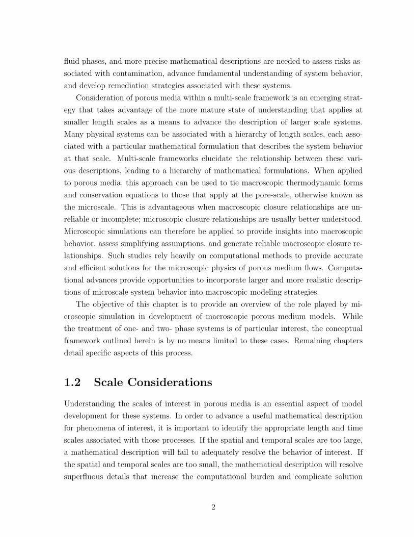
fluid phases, and more precise mathematical descriptions are needed to assess risks as-

sociated with contamination, advance fundamental understanding of system behavior,

and develop remediation strategies associated with these systems.

Consideration of porous media within a multi-scale framework is an emerging strat-

egy that takes advantage of the more mature state of understanding that applies at

smaller length scales as a means to advance the description of larger scale systems.

Many physical systems can be associated with a hierarchy of length scales, each asso-

ciated with a particular mathematical formulation that describes the system behavior

at that scale. Multi-scale frameworks elucidate the relationship between these vari-

ous descriptions, leading to a hierarchy of mathematical formulations. When applied

to porous media, this approach can be used to tie macroscopic thermodynamic forms

and conservation equations to those that apply at the pore-scale, otherwise known as

the microscale. This is advantageous when macroscopic closure relationships are un-

reliable or incomplete; microscopic closure relationships are usually better understood.

Microscopic simulations can therefore be applied to provide insights into macroscopic

behavior, assess simplifying assumptions, and generate reliable macroscopic closure re-

lationships. Such studies rely heavily on computational methods to provide accurate

and efficient solutions for the microscopic physics of porous medium flows. Computa-

tional advances provide opportunities to incorporate larger and more realistic descrip-

tions of microscale system behavior into macroscopic modeling strategies.

The objective of this chapter is to provide an overview of the role played by mi-

croscopic simulation in development of macroscopic porous medium models. While

the treatment of one- and two- phase systems is of particular interest, the conceptual

framework outlined herein is by no means limited to these cases. Remaining chapters

detail specific aspects of this process.

1.2 Scale Considerations

Understanding the scales of interest in porous media is an essential aspect of model

development for these systems. In order to advance a useful mathematical description

for phenomena of interest, it is important to identify the appropriate length and time

scales associated with those processes. If the spatial and temporal scales are too large,

a mathematical description will fail to adequately resolve the behavior of interest. If

the spatial and temporal scales are too small, the mathematical description will resolve

superfluous details that increase the computational burden and complicate solution

2

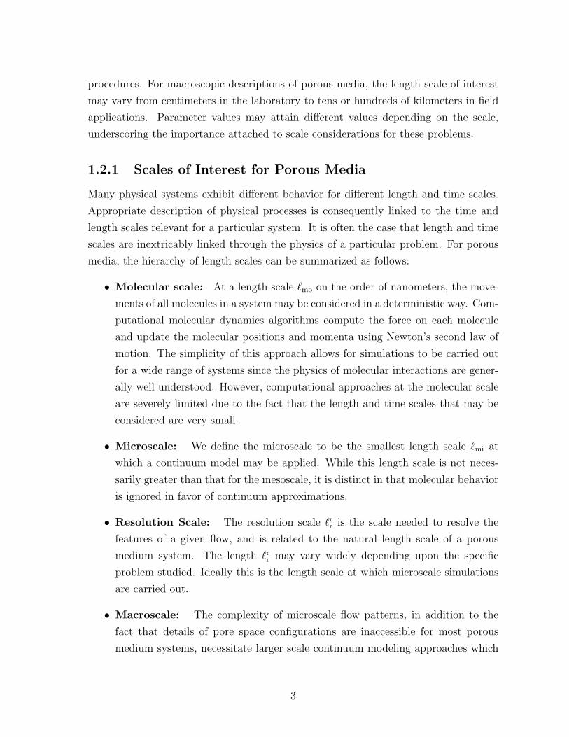
procedures. For macroscopic descriptions of porous media, the length scale of interest

may vary from centimeters in the laboratory to tens or hundreds of kilometers in field

applications. Parameter values may attain different values depending on the scale,

underscoring the importance attached to scale considerations for these problems.

1.2.1 Scales of Interest for Porous Media

Many physical systems exhibit different behavior for different length and time scales.

Appropriate description of physical processes is consequently linked to the time and

length scales relevant for a particular system. It is often the case that length and time

scales are inextricably linked through the physics of a particular problem. For porous

media, the hierarchy of length scales can be summarized as follows:

• Molecular scale: At a length scale `mo on the order of nanometers, the move-

ments of all molecules in a system may be considered in a deterministic way. Com-

putational molecular dynamics algorithms compute the force on each molecule

and update the molecular positions and momenta using Newton’s second law of

motion. The simplicity of this approach allows for simulations to be carried out

for a wide range of systems since the physics of molecular interactions are gener-

ally well understood. However, computational approaches at the molecular scale

are severely limited due to the fact that the length and time scales that may be

considered are very small.

• Microscale: We define the microscale to be the smallest length scale `mi at

which a continuum model may be applied. While this length scale is not neces-

sarily greater than that for the mesoscale, it is distinct in that molecular behavior

is ignored in favor of continuum approximations.

• Resolution Scale: The resolution scale `rr is the scale needed to resolve the

features of a given flow, and is related to the natural length scale of a porous

medium system. The length `rr may vary widely depending upon the specific

problem studied. Ideally this is the length scale at which microscale simulations

are carried out.

• Macroscale: The complexity of microscale flow patterns, in addition to the

fact that details of pore space configurations are inaccessible for most porous

medium systems, necessitate larger scale continuum modeling approaches which

3

describe the behavior in an average sense. This approach has the advantage of

neglecting many smaller scale details that do not ultimately effect transport at

the larger scale. The macroscale is the length scale `ma at which the properties

of this larger system are invariant with respect to system size. The goal of most

microscale approaches is to simulate a domain large enough to achieve the lower

end of this scale.

It is clear that for a given system `mo < `mi < `rr < `ma. Additionally, sub-molecular

length scales can be important when quantum mechanical effects are significant, and at

larger macroscopic length scales (sometimes called field scale, regional scale or megas-

cale) can be important, especially when large-scale heterogeneity must be accounted

for. Consideration of the issues associated with these systems is beyond the scope of

this work.

1.2.2 Microscale Simulation and Macroscale Model Develop-

ment

The hierarchy of length scales can be exploited within a multi-scale framework by devel-

oping strategies to transfer information between spatial scales. The primary objective

of a multi-scale simulation framework is to use microscale simulation data to generate

insights about system behavior at the macroscale. Length-scale considerations are in-

timately tied to computational cost for most simulation procedures, and simulations

must be sufficiently large to bridge the gap between spatial scales. An appropriate

theoretical framework is also a necessity; in order to transfer information from the

microscale to the macroscale, the relationships among respective variables must be ex-

plicitly defined. This requirement is discussed further in §1.3.1. Provided that the

details of the microscale system are known, the macroscopic system may be computed

directly. Hence a given micro-state will correspond with exactly one macro-state. The

converse is not true, as a given macroscopic state will often correspond with infinitely

many micro-states. This is indicative of loss of microscopic detail associated with the

macroscopic formulation. In practice, this information is not omitted entirely, instead

aspects are reconstituted in the form of constitutive laws.

Multi-scale simulation approaches generally fall within two categories: (1) direct

approaches in which information from a larger scale simulation is used to initialize a

simulation performed at a smaller scale, which in turn returns information directly to

the larger scale simulation; (2) indirect approaches in which microscopic simulations

4

are used to quantify constitutive laws relating macroscopic variables. As the direct

approach relies on the larger scale simulation to initialize the smaller scale simula-

tion, their application is primarily heuristic; it would be straightforward to replace the

small scale simulation with a derived constitutive law. Since microscale simulations are

computationally expensive, constitutive laws provide an efficient way to incorporate

microscale simulation data into macroscopic forms that allow simulation data to be

reused many times.

In recent years, microscale study of porous medium systems has expanded consid-

erably. This is in large part due to computational advances that now provide access

to simulations of sufficiently large, three-dimensional domains as necessary to obtain

results that are extensible to macroscopic systems. In addition to the development of

constitutive laws, microscale studies provide opportunities to consider macroscopic sys-

tems in the absence of simplifying assumptions, access information that is not available

from macroscopic approaches, and improve conceptual understanding of system behav-

ior. Where macroscopic descriptions are incomplete, microscale information provides

a platform to study assumptions and approximations related to their establishment.

In cases in where macroscopic model forms are relatively well established, microscale

information can be used to expand the range of validity for these forms and estimate

associated macroscopic model parameters. Particular attention has been paid to mi-

croscale study of multiphase systems. Significant gaps are present in our understanding

of macroscopic multiphase systems, particularly concerning the proper description of

thermodynamic forms [66, 68, 70, 69, 57]. Although open questions remain even at the

microscale, thermodynamic forms and constitutive laws are more well established and

allow for useful simulation [49, 132, 91, 103, 170].

1.2.3 Sources of Microscale Information

Network Modeling

Developing a computationally tractable simulation procedure which can be used to

study macroscopic behavior while adequately describing flow processes in porous media

is one of the principle challenges to the computational study of microscopic porous

medium systems. In order to obtain realistic insights into macroscopic behavior, large

domains must be considered. Network models construct idealized approximations of

the pore space so that flow processes are described by simple analytical expressions.

These simplifications allow for the consideration of much larger systems than what

5

could be considered using other methods. Network models have been extended to

consider a wide range of porous medium systems [28, 171, 46, 20, 45, 2]. However, the

simplified physics and pore structure significantly limit the utility of these approaches,

particularly as computational capabilities increase the viability of alternative simulation

procedures.

Lattice Boltzmann Modeling

Direct simulation of fluid flows in realistic porous media is a computational intensive

process. Traditional fluid mechanics approaches are not well-suited to dealing with

the complexity of solid boundaries and fluid interfaces present in porous media. The

lattice Boltzmann method has become a primary tool for simulation of porous medium

flows in part due to the simplicity by which fluid and solid interfaces are treated.

Porous medium calculations are routinely performed for single- and multiphase systems

[137, 175, 138, 139, 150, 159, 167, 148]. A proliferation of multiphase lattice Boltzmann

schemes have resulted from the desire to increase physical accuracy and to expand the

range of systems that can be considered using this approach [33, 74, 84, 100, 85, 122,

101, 86, 102, 47, 96, 172]. Schemes have been devised to model a wide range of physical

phenomena in addition to single- and multi-phase flows, particularly approaches to

simulate transport of fluids and dissolved components and with consideration of reactive

transport [178, 9, 93, 10, 8, 11, 92].

Computed Micro-Tomography

Tomographic imaging provides a non-invasive way to obtain high-resolution, three-

dimensional images of real porous medium systems. This approach can be used to

generate hi-resolution images of real porous medium systems, and is most typically used

to obtain images of equilibrium configurations in multiphase porous media [80, 37, 191,

188, 192, 190, 3, 162, 189, 149]. A primary limitation of tomographic imaging is that

dynamic information is typically inaccessible, limiting studies to cases of mechanical

equilibrium.

6

1.3 Macroscopic Modeling Approaches for Porous

Media

Porous medium models are typically formulated at sufficiently large length scales so that

any microscopic dynamics that do not directly impact the macroscopic behavior can be

neglected. While such formulations are properly considered as averages of the micro-

scopic behavior, many existing porous medium models have been constructed without

giving due consideration to the definitions of derived variables, particularly those which

pertain to thermodynamics. Traditional models are often applied outside their range of

validity, are plagued by unrealistic or oversimplified assumptions regarding system be-

havior, and suffer from the lack of a sufficiently general modeling framework to provide

guidance when models fail. In order to overcome these shortcomings, it is necessary to

consider alternative strategies to produce the rigorous and flexible models needed to

accurately describe the behavior of porous medium systems. Given that systems are

usually better understood at smaller scales, it is logical to develop models by establish-

ing a connection to smaller scale physics. In this section, we review the typical model

formulations applied to describe single- and multi-phase systems in porous media, and

provide an introduction to thermodynamically constrained averaging theory as a means

to generate more reliable models.

Traditional Model Formulation for Single Phase Systems

For the case of a porous medium is fully saturated with a single fluid phase, flow

behavior is typically described using Darcy’s law. Darcy’s law was initially obtained

as an empirical expression relating the total change in head h across a system with the

volumetric flow rate [41]. This expression has been generalized into a differential form

with which Darcy’s law has become synonymous:

εαvα = −K · ∇h, (1.1)

where εα is the volume fraction of the fluid, vα is the flow velocity, and K is the

permeability tensor for the porous media. Expressions such as Eq. (1.1) have been

applied broadly, well beyond the range of support of the original experiments [58].

Subsequently, theoretical approaches have succeeded in deriving Darcy’s law from first

principles, which has provided more precise definitions for the variables appearing in

Eq. (1.1) as well as insights in to its range of validity [184, 60]. Such approaches have

7

also been used to derive extensions to Darcy’s law, such as the Forchheimer equation

[152, 153, 185]. These expressions are widely used, and generally considered to be

useful.

Systems containing a single fluid phase within the solid matrix are typically de-

scribed by inserting a differential form of Darcy’s law into an equation for conservation

of mass formulated at the macroscale:

∂(ραεα)

∂t+∇·(ραεαvα) = 0, (1.2)

where ρα is the fluid density. By inserting Eq. (1.1) into Eq. (1.2) and applying various

approximations, one obtains the standard equations used to model single phase flow

in porous media [16]. While these approaches are generally effective, there is some

cause for concern. For example, by formulating conservation principles directly at the

macroscale the precise definitions of quantities appearing in Eq. (1.2) are obscured [58].

Although the physical meaning of these variables may be intuitive, this still presents

a problem because the relationship among variables appearing in the mathematical

formulation and variables which are actually measured is not clear. In order to resolve

this issue, it is necessary to provide additional information so that the relationship

among variables at different scales is clear.

Model Formulation for Multiphase Systems

The standard mathematical formulation for description of multiphase systems is similar

to the single phase formulation, constructed by inserting an extension of Darcy’s law

into the mass conservation equation given by Eq. (1.2) for each phase α. For the

multiphase formulation, the extension to Darcy’s law is given by [29]:

εαvα = −κκαr

µα(∇pα − ραgα). (1.3)

New quantities introduced in this equation are the intrinsic permeability κ, the dynamic

viscosity µα, the fluid pressure pα, and the gravitational acceleration gα. The relative

permeability καr is included to account for the effective change in permeability due to

the presence of additional fluid phases. While theoretical work exists to support the

single phase form of Darcy’s law, no sound theoretical approach has been used to justify

the multiphase extension given by Eq. (1.3). In fact, limitations associated with this

formulation are widely recognized and its inclusion is largely attributable to the lack

8

of a suitable alternative [130, 83, 79]. An inherent limitation of this approximation

is that Eq. (1.3) serves as a replacement for a formal momentum equation, yet offers

no mechanism to include the effects of potentially important processes such as viscous

coupling between the fluid phases present in the system [12, 13, 14, 15, 104].

An additional problem has been introduced into the multiphase flow formulation due

to the fact that the fluid pressure and relative permeability for each phase are unknown.

In order to close this equation, constitutive laws are introduced in which pα and καr are

provided as functions of known variables. In most cases, it assumed that both variables

are functions of the fluid saturation εα/εs alone. In each case, the existence of such

a functional relationship has been called into question. In many instances, pα and καr

will depend on other variables, such as interfacial area. Ignoring these dependencies

leads to hysteresis in derived constitutive relations [23, 24, 25, 22, 26, 21, 104, 163,

155]. Accurate description of multiphase systems cannot be accomplished without

an appropriate deterministic set of macroscopic variables. Pore-scale studies are an

essential tool for identification of these variables and quantification of the associated

relationships [39, 154, 65, 76, 30, 109, 119, 120, 151]

1.3.1 Thermodynamically Constrained Averaging Theory

Thermodynamically constrained averaging theory (TCAT), provides a systematic ap-

proach for obtaining porous medium flow models models, This framework has been used

to advance approaches to model flow and transport for a wide range of systems. In

order to construct a macroscopic description of particular system, macroscopic conser-

vation equations, thermodynamic forms, and an entropy inequality are constructed by

averaging their microscopic counterparts. This ensures that macroscopic variables are

rigorously defined in terms of microscale variables, eliminating ambiguity with respect

to these variables [59, 127, 60, 129, 62, 87, 61, 63]. This framework provides solutions

to many of the shortcomings associated with traditional modeling approaches:

• Macroscale variables are rigorously defined;

• Firm connection of scales;

• Flexible modeling framework;

• Constrained by 2nd law of thermodynamics;

9

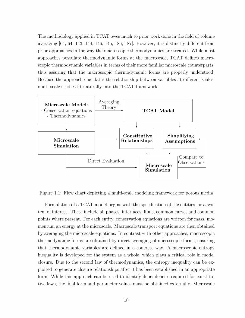
The methodology applied in TCAT owes much to prior work done in the field of volume

averaging [64, 64, 143, 144, 146, 145, 186, 187]. However, it is distinctly different from

prior approaches in the way the macroscopic thermodynamics are treated. While most

approaches postulate thermodynamic forms at the macroscale, TCAT defines macro-

scopic thermodynamic variables in terms of their more familiar microscale counterparts,

thus assuring that the macroscopic thermodynamic forms are properly understood.

Because the approach elucidates the relationship between variables at different scales,

multi-scale studies fit naturally into the TCAT framework.

Microscale Model:- Conservation equations

- Thermodynamics

?

MicroscaleSimulation

Direct Evaluation-

-

-

AveragingTheory

TCAT Model

??

SimplifyingAssumptions

ConstitutiveRelationships

MacroscaleSimulation

? ?Compare toObservations

Figure 1.1: Flow chart depicting a multi-scale modeling framework for porous media

Formulation of a TCAT model begins with the specification of the entities for a sys-

tem of interest. These include all phases, interfaces, films, common curves and common

points where present. For each entity, conservation equations are written for mass, mo-

mentum an energy at the microscale. Macroscale transport equations are then obtained

by averaging the microscale equations. In contrast with other approaches, macroscopic

thermodynamic forms are obtained by direct averaging of microscopic forms, ensuring

that thermodynamic variables are defined in a concrete way. A macroscopic entropy

inequality is developed for the system as a whole, which plays a critical role in model

closure. Due to the second law of thermodynamics, the entropy inequality can be ex-

ploited to generate closure relationships after it has been established in an appropriate

form. While this approach can be used to identify dependencies required for constitu-

tive laws, the final form and parameter values must be obtained externally. Microscale

10

simulation is a natural candidate to finalize constitutive laws because a wide range

of systems may be considered and local values of microscopic variables are known,

permitting computation of their macroscopic counterparts.

1.4 Research Objectives

Microscopic simulation can play a vital role in the development of macroscopic porous

medium models. Construction of appropriate numerical tools is an essential aspect of

constitutive law development. The objective of this document is to detail the devel-

opment of microscale simulation and analysis tools, to evaluate the viability of these

tools for various porous medium simulation scenarios, and to advance the state of un-

derstanding for macroscopic flow processes using simulation and analysis.

The specific research objectives to be accomplished are as follows:

1. High performance parallel lattice Boltzmann schemes targeted toward microscale

simulation of one and two phase flows in porous media;

2. Construct a comprehensive set of tools designed to accurately measure geometric

and morphological properties from real and simulated data sets;

3. Demonstrate insufficiencies in the form of momentum approximations used to

describe non-Darcy flow in anisotropic porous media and demonstrate how TCAT

can be used to guide the construction of extended models.

11

Chapter 2

High Performance Implementations

of the Lattice Boltzmann Method

2.1 Introduction

The lattice Boltzmann Method (LBM) occupies a prominent role in the development

of porous medium flow and transport models. The principal objective of associated

pore-scale study is to advance understanding of macroscopic system behavior such

that the microscopic details of flow can be neglected. In such cases critical aspects of

the microscopic physics must be provided to macroscopic model formulations in the

form of closure relations [59]. Pore-scale simulation provides a mechanism to study

these relations provided that simulations are able to accommodate the complex solid

morphology and large domain sizes needed to produce results that can be scaled to a

macroscopically significant length scale, and to resolve adequately the relevant physical

mechanisms.

The LBM is well-suited to simulation of porous medium flows and has become

a primary tool for simulation of single- and multiphase flow in porous media. The

significance of this role is evidenced by widespread efforts to evaluate and predict porous

medium permeability values for single-phase flows based on microscopic simulation [115,

137, 166, 164]. LBM investigations of multiphase flow behavior represent an even more

important niche due to well-documented deficiencies in existing macroscopic model

formulations [126, 87]. Widely used constitutive relationships relating capillary pressure

and saturation exhibit strong hysteresis, an effect which is being actively studied using

the LBM [138, 104, 159, 168, 1]. The necessity for large, efficient simulations motivates

the development of scalable parallel implementations, which allow for the simulation of

larger scale systems than would be possible on single processor or even a single node

with multiple processing cores.

Achieving high performance requires concurrency for the computations performed

at all levels of hierarchically organized parallel computing systems. This objective

has been investigated in detail for distributed memory systems, for which concurrent

computations can be achieved by subdividing computations between processors by con-

structing an appropriate domain decomposition strategy [140, 182, 181, 179]. Trends in

processor design are establishing new paradigms for LBM computing. Individual pro-

cessor speeds are no longer increasing at a rapid rate and hardware-based acceleration

therefore hinges on exploiting multiprocessing throughout the hierarchical structure of

modern parallel computing systems [72]. LBM’s are particularly challenging since their

performance is dominated by memory bandwidth that does not always scale uniformly

with the number of processors in many modern architectures [77]. Newer developments

address this bottleneck, which have not been fully tested in parallel implementations of

the LBM. Graphics processing units (GPU’s) have become a popular target for acceler-

ating the LBM due to their high-memory bandwidth and performance that scales well

with the number of processor cores and often outperform CPU’s for memory-limited

computations [50]. In recent years, the capabilities and tools associated with computa-

tional science applications on GPU’s have evolved rapidly. GPU implementations have

been associated with significant speedup for single-component, 3-D implementations of

the LBM [135, 50, 174, 95, 180, 98]. Myre et. al. found that this high performance can

be scaled to multiple GPU’s for both single and multiple component implementations

of the LBM [131].

Algorithm advancements and hardware evolution have important ramifications for

porous medium flow simulations. Unfortunately, many performance studies have fo-

cused exclusively on implementations that utilize a simple BGK approach for single

fluid component systems. More computationally intensive multi-relaxation time (MRT)

schemes are essential to reproduce accurately certain aspects of the fluid physics, and

performance results for the BGK scheme are not representative of such methods [139].

Assessments of parallel performance often make use of outdated data structures and

algorithms such that scaling results are derived from serial code that is not optimal.

Furthermore, many advanced algorithms and data structures have not been considered

in the context of the multi-component schemes typically used to study multiphase flow,

which impose both higher computational demands and more complex algorithmic con-

straints. The extension of state-of-the-art algorithms to the simulation of multiphase

13

flow in porous medium systems has not been detailed in the literature. Furthermore,

the range of problems that can and cannot be addressed, even using the very best meth-

ods, have not been considered in the literature. Lastly, physical mechanisms manifest

in multiphase porous medium systems pose special challenges that have not yet been

sufficiently documented in the literature.

The overall goal of this work is to advance LBM modeling of multiphase flow in

porous medium systems. The specific objectives of this work are: (1) to detail the for-

mulation of state-of-the-art algorithms for LBM modeling of multiphase flow in porous

medium systems; (2) to illustrate approaches that produce an efficient simulator on

a single processor; (3) to summarize methods needed to produce a multiphase LBM

simulator that scales well across multiple processors; (4) to extend a state-of-the art

multiphase LBM to a GPU computing environment; (5) to derive limits on the scale of

multiphase LBM simulations that are feasible using efficient methods as a function of

the computing resources available; and (6) to illustrate challenges remaining to simulate

efficiently, and with high fidelity, multiphase flow in porous medium systems.

2.2 Methods

2.2.1 Model Problems for Porous Media

Microscale simulation of flow in porous media requires detailed knowledge of pore struc-

ture in order to provide boundary conditions to the LBM. This information is usually

obtained either by using advanced imaging techniques to obtain a three-dimensional

picture of a real porous medium system or by generating a synthetic representation of

a porous medium system [191, 192, 190, 162]. In this work, surrogate porous media

are constructed by generating random close packings of equally-sized spheres [194]. All

media considered have a porosity of 0.369, slightly above the known minimum value.

A packing of 128,000 spheres is shown in Fig. (3.14). Sphere packings are provided to

the LBM code in digitized form, with D being the diameter of each sphere expressed

in lattice units.

2.2.2 Permeability Measurement

Permeability measurement has become a standard calculation for the LBM in porous

media. For sufficiently small flow rates, the 1-D macroscopic flow behavior obeys

14

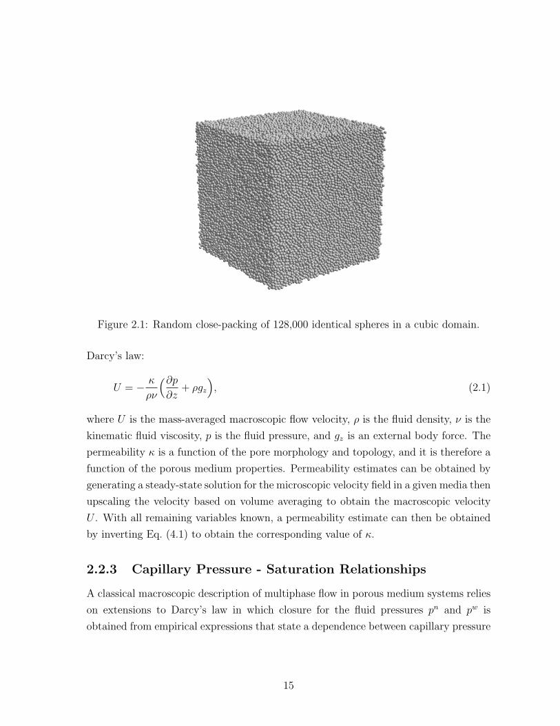
Figure 2.1: Random close-packing of 128,000 identical spheres in a cubic domain.

Darcy’s law:

U = − κ

ρν

(∂p∂z

+ ρgz

), (2.1)

where U is the mass-averaged macroscopic flow velocity, ρ is the fluid density, ν is the

kinematic fluid viscosity, p is the fluid pressure, and gz is an external body force. The

permeability κ is a function of the pore morphology and topology, and it is therefore a

function of the porous medium properties. Permeability estimates can be obtained by

generating a steady-state solution for the microscopic velocity field in a given media then

upscaling the velocity based on volume averaging to obtain the macroscopic velocity

U . With all remaining variables known, a permeability estimate can then be obtained

by inverting Eq. (4.1) to obtain the corresponding value of κ.

2.2.3 Capillary Pressure - Saturation Relationships

A classical macroscopic description of multiphase flow in porous medium systems relies

on extensions to Darcy’s law in which closure for the fluid pressures pn and pw is

obtained from empirical expressions that state a dependence between capillary pressure

15

pc and fluid saturation sw:

pn − pw = pc(sw). (2.2)

The mathematical form of this relationship was first investigated experimentally. In a

typical experimental setup, reservoirs of wetting and non-wetting fluids are established

on opposite sides of the domain, and flow of the two fluids is controlled by varying

the capillary pressure difference pc as determined by the pressure difference between

the fluid reservoirs [110]. Problematically, the relationship stated in Eq. (2.2) depends

on the system history, an effect that is due, at least in part, to the dependence of the

relationship on typically neglected variables such as specific interfacial areas, specific

common curve lengths, and average interfacial curvatures [70, 87]. Lattice Boltzmann

investigations into multiphase behavior are of interest because they provide a straight-

forward way to evaluate microscale properties directly from highly resolved pore-scale

simulations [148].

2.2.4 LBM Fundamentals

The LBM can be used to model a wide range of physical systems that are of interest

to the study of porous media. From an implementation standpoint, these schemes

share much in common. In this work, we consider schemes that utilize a three-

dimensional, nineteen velocity vector (D3Q19) structure. For the planes in the x-,

y- and z- directions, the D3Q19 structure matches the velocity structure of the familiar

two-dimensional, nine velocity vector (D2Q9) model. The computational domain Ω is

defined by a rectangular prism discretized to obtain regularly spaced lattice sites xi

where i = 0, 1, . . . , N − 1, N = Nx ×Ny ×Nz. The number of lattice sites in the x, y

and z directions are denoted as Nx, Ny and Nz. For the D3Q19 velocity structure, the

microscopic velocity space is discretized to include 19 discrete velocities [73]

ξq =

0, 0, 0T for q = 0

±1, 0, 0T , 0,±1, 0T , 0, 0,±1T for q = 1, 2, . . . , 6

±1,±1, 0T , ±1, 0,±1T , 0,±1,±1T for q = 7, 8, . . . , 18.

(2.3)

A set of discrete distributions fαq is constructed to track the fluid behavior for each fluid

component α ∈ E, where the component set E is model specific. For each component,

16

the density and velocity are obtained directly from the discrete distributions

ρα =

Q−1∑q=0

fαq , (2.4)

uα =1

ρα

Q−1∑q=0

ξqfαq . (2.5)

The total density and average velocity are obtained by summing over all components

ρ =∑α∈E

ρα, (2.6)

u =1

ρ

∑α∈E

ραuα. (2.7)

Since density and velocity can be obtained directly from the distributions, a nu-

merical solution for fαq implies a solution for ρα and uα. This solution is obtained by

solving the lattice Boltzmann equation, which may be expressed in the general form

fαq (xi + ξq, t+ 1)− fαq (xi, t) = Cαq. (2.8)

The model-specific collision operator Cαq accounts for changes in fαq due to the inter-

molecular interactions and collisions. The collision term depends only on local values

of the distributions, but may depend non-locally on conserved moments of the dis-

tributions. Solution of Eq. (2.8) is usually accomplished in two steps, referred to as

streaming

fα∗q (xi + ξq, t+ 1) = fαq (xi, t), (2.9)

and collision, which accounts for molecular collision and interaction

fαq (xi, t+ 1) = fα∗q (xi, t+ 1) + Cα∗q. (2.10)

The streaming step defined by Eq. (2.9) propagates the distributions on the lattice,

a process that depends only on the discrete velocity set ξq. Since streaming is in-

dependent of the model-specific collision operator Cαq, optimization of the streaming

step depends only on the velocity structure and the number of components. For all

models considered in this work, the solid phase is assumed immobile and boundary

conditions are prescribed by the bounce-back rule [54]. To explore the optimization of

17

LBM methods, we consider three common approaches used to simulate flow in porous

medium systems. Collision structures for the BGK, MRT and Shan-Chen schemes are

given below, and implementation and optimization details are provided in §2.3.

Single-Component BGK Model

The simple BGK model remains a widely applied collision rule for the LBM [89, 118,

114, 88, 133]. For a single component w, this approximation assumes that the distri-

butions relax at a constant rate toward equilibrium values f eq,wq prescribed from the

Maxwellian distribution [73]:

Cwq =1

τw(f eq,wq − fwq

). (2.11)

The relaxation rate is specified by the parameter τw > 0.5, known as the relaxation

time, which is related to the kinematic viscosity of the fluid:

ν =1

3

(τ − 1

2

). (2.12)

Based on a quadrature scheme for the Maxwellian distribution, the equilibrium distri-

butions take the form:

f eq,wq = wqρw[1 + 3(ξq·uw) + 9

2(ξq·uw)2 − 3

2(uw·uw)

], (2.13)

where w0 = 1/3, w1,...,6 = 1/18 and w7,...,18 = 1/36. In choosing the equilibrium

distributions, conservation of the fluid density ρw and momentum jw = ρwuw is ensured

by:

ρw =

Q−1∑q=0

fwq =

Q−1∑q=0

f eq,wq , (2.14)

jw =

Q−1∑q=0

ξqfwq =

Q−1∑q=0

ξqfeq,wq . (2.15)

2.2.5 Single-Component Multi-Relaxation Time Model

In the BGK approximation to the collision term as given by Eq. (2.11), all non-conserved

hydrodynamic modes relax toward equilibrium at the same rate, specified by the re-

laxation time τw. Multi-relaxation time (MRT) schemes are constructed such that

18

different hydrodynamic modes relax at different rates. Many physically significant

hydrodynamic modes are associated with linear combinations of the distributions fwq[99, 44]:

fwm =

Q−1∑q=0

Mm,qfwq , (2.16)

where Mm,q represents a set of constant coefficients associated with a particular mode

m. Since there are Q independent, linear combinations of fwq , coefficients are defined

for m = 0, 1, 2, . . . , Q− 1. The coefficients must be chosen carefully in order to ensure

that moments correspond with physical modes that are hydrodynamically significant.

Based on the approach of d’Humieres and Ginzburg [44], the coefficients Mm,q are

obtained by applying a Gram-Schmidt orthogonalization to polynomials of the discrete

velocities ξq. The resulting set of moments include density, momentum, and kinetic

energy modes, as well as modes associated with elements of the stress tensor. Once the

transformation coefficients are known, the relaxation process is carried out in moment

space, with each mode relaxing at its own rate specified by λwm:

Cwq =

Q−1∑m=0

M∗q,mλ

wm

(f eq,wm − fwm

). (2.17)

The inverse transformation coefficients M∗q,m map the moments back to distribution

space, and are obtained by applying a matrix inverse using the values of the transfor-

mation coefficients, Mm,q. In the MRT formulation, the equilibrium moments f eq,wm are

functions of the local density ρw and momentum jw. In order to minimize the depen-

dence of the permeability on the solid wall location, the relaxation parameters take the

form [139]:

λw1 = λw2 = λw9 = λw10 = λw11 = λw12 = λw13 = λw14 = λw15 =1

τw, (2.18)

λw4 = λw6 = λw8 = λw16 = λw17 = λw18 =8(2− λw1 )

8− λα1. (2.19)

Since the density and momentum modes do not undergo relaxation, there is no need

to specify relaxation parameters for the associated moments.

19

2.2.6 Multi-Component Shan-Chen MRT Model

Description of multi-component mixtures and immiscible fluid flows, which is the focus

of this work, can be accomplished by introducing modified collision operations, which

account for these interactions. While a number of schemes have been constructed to

achieve this purpose, the Shan-Chen scheme represents the simplest and most widely-

used approach for simulating multi-component flows in porous media. We consider the

Shan-Chen model for binary mixtures, E = w, n. In this approach, a quasi-molecular

interaction force is introduced to approximate the force acting on component α due to

component β:

Fα(xi, t) = ρα(xi, t)

Q−1∑q=1

Gwnρβ(xi − ξq, t)ξq, α, β ∈ w, n, α 6= β. (2.20)

The parameter Gwn determines miscibility and surface tension between the wetting and

non-wetting components w and n. An analogous force is introduced to account for

interactions between the solid and fluid phases. In practice, this may be achieved with

appropriate assignment of the density values within the solid phase:

ρw(xi) =Gs

Gwnfor xi ∈ Ωs, (2.21)

ρn(xi) = − Gs

Gwnfor xi ∈ Ωs. (2.22)

The fluid-solid interaction parameter Gs > 0 can be tuned to determine the contact

angle [81].

Interfacial forces are incorporated by considering their effect on the fluid momentum.

Due to this choice, momentum is no longer conserved locally and a relaxation process

must be introduced for the associated moments. The common velocity u′ is defined as:

u′ =

∑α=w,n

jα∑α=w,n

ρα. (2.23)

The post-collision momentum is then defined as:

j′α = ραu′ + Fα. (2.24)

The equilibrium moments are computed in terms of the post-collision momentum j′α to

20

define the collision process for the Shan-Chen model. Since Eq. (2.20) is non-local in

terms of the fluid densities, both the streaming step and density computation must be

performed prior to collision in order to ensure that the collision step is implicit in terms

of the component densities. Unlike the single-component MRT scheme, momentum is

not conserved locally in the Shan-Chen LBM. This means that the momentum modes

undergo relaxation, and the full set of relaxation parameters used in this work are:

λα3 = λα5 = λα7 = 1, (2.25)

λα1 = λα2 = λα9 = λα10 = λα11 = λα12 = λα13 = λα14 = λα15 =1

τα, (2.26)

λα4 = λα6 = λα8 = λα16 = λα17 = λα18 =8(2− λα1 )

8− λα1. (2.27)

2.3 Implementation and Optimization Approaches

Computational performance for the LBM is determined primarily from two factors:

(1) the number of arithmetic operations that must be performed, and (2) the amount

of data to be moved between processors and memory. The former is determined by

the processor clock speed and instruction set, whereas the latter is limited by memory

bandwidth. Performance of the LBM relies heavily on memory bandwidth due to the

large number of variables that must be accessed from arrays to perform each lattice

update [7, 6]. LBM’s exhibit poor temporal locality of data — each distribution fαq

computed in the collision step at each lattice site is used just once in the streaming step.

For single component schemes, performance is strongly linked to the streaming step

implementation, which can be accomplished by implementing one of several existing

algorithms [117]. Performance of the LBM is also sensitive to the lattice structure and

access patterns, an effect which can be traced to spatial locality of the distributions

needed in the collision step [193, 183, 198]. Domain decomposition and communication

overlap is essential to generate efficient parallel implementations [140, 182, 181, 179].

Careful consideration of all these aspects are needed to produce an efficient simulator.

Two measures of efficiency are especially important: (1) the number of lattice up-

dates per second that can be computed, and (2) how the lattice update rate scales

with the number of processors allocated for the computation. Achieving high efficiency

is critical because many multiphase LBM simulations of porous medium problems of

concern are at, or beyond, current computational limits for even the most advanced

computers.

21

We focus our discussion on the most critical aspects of the hardware, and summarize

algorithms that have been shown to yield excellent performance. We also provide imple-

mentation guidance to enable others to more readily develop efficient LBM simulators.

Specifically we address hardware considerations, serial CPU optimization, parallel CPU

optimization, and GPU optimization.

2.3.1 Hardware Overview

Scalable parallel computers combine multiple CPU’s sharing memory into a node, and

interconnect multiple nodes through a high speed switching network into a cluster.

Fig. (2.2) illustrates the structure of a single node in a parallel computing cluster circa

2010. An Intel node based on four Nehalem-EX processors is illustrated; similar designs

are available from other manufacturers (e.g. based on AMD opteron or IBM Power

components). Each Nehalem-EX processor contains 8 parallel processing cores, and

can reference directly attached high-speed memory at about 40 GB/s. It also connects

directly to the other three processors through a high speed interconnect (100GB/s) to

access non-local memory. In aggregate, this configuration provides 32 processing cores

with up to 160 GB/s of shared main memory bandwidth. Computational accelerators,

in the form of graphics processing units can also be incorporated in the node. Data is

transferred to and from the GPUs at about 4–8 GB/s. Data is transferred to and from

other nodes in the cluster at about the same rate (4–8 GB/s).

Multiple levels of cache are provided to reduce the latency associated with memory

accesses. Depending on the specific processor, a particular data cache may be associated

with each individual core or may be shared between multiple cores. For the setup shown

in Fig. (2.2), each of the eight cores in a Nehalem-EX is equipped with 32 KB dedicated

L1 data cache and 256 KB L2 cache. A 24 MB L3 cache is shared among the eight cores.

Each cache stores a subset of the data contained within main memory based on which

data is required by the processor cores to perform computations. The time to access

data from the caches is considerably lower than the time to access data from main

memory. Once data has been loaded into the cache, it remains there until subsequent

data accesses require it to be replaced. Temporal and spatial locality of cache references

can be improved by manipulating data access patterns, which can impact performance

significantly. Relatively little temporal locality is presented by LBM methods.

While the processor cores on a multi-core CPU are capable of performing computa-

tions in parallel, serial codes use only one core at a time and therefore do not take full

22

MemoryModule

GPUGPUGPUGPU

I/O

I/O

Hub

Hub

Nehalem

Nehalem Nehalem

Nehalem

EX

EX EX

EX

Network Connectionto Other Nodes

Figure 2.2: Schematic showing a GPU-accelerated processing node populated with fourIntel Nehalem Xeon CPU’s, each with 8 processing cores.

23

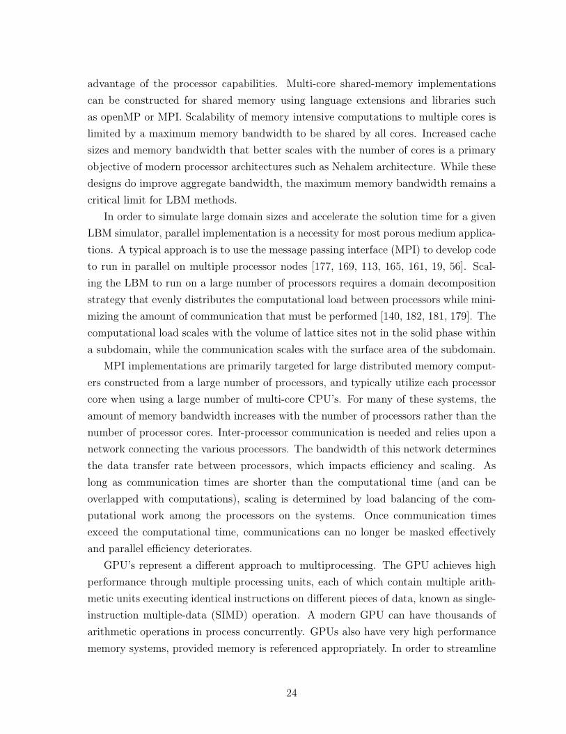
advantage of the processor capabilities. Multi-core shared-memory implementations

can be constructed for shared memory using language extensions and libraries such

as openMP or MPI. Scalability of memory intensive computations to multiple cores is

limited by a maximum memory bandwidth to be shared by all cores. Increased cache

sizes and memory bandwidth that better scales with the number of cores is a primary

objective of modern processor architectures such as Nehalem architecture. While these

designs do improve aggregate bandwidth, the maximum memory bandwidth remains a

critical limit for LBM methods.

In order to simulate large domain sizes and accelerate the solution time for a given

LBM simulator, parallel implementation is a necessity for most porous medium applica-

tions. A typical approach is to use the message passing interface (MPI) to develop code

to run in parallel on multiple processor nodes [177, 169, 113, 165, 161, 19, 56]. Scal-

ing the LBM to run on a large number of processors requires a domain decomposition

strategy that evenly distributes the computational load between processors while mini-

mizing the amount of communication that must be performed [140, 182, 181, 179]. The

computational load scales with the volume of lattice sites not in the solid phase within

a subdomain, while the communication scales with the surface area of the subdomain.

MPI implementations are primarily targeted for large distributed memory comput-

ers constructed from a large number of processors, and typically utilize each processor

core when using a large number of multi-core CPU’s. For many of these systems, the

amount of memory bandwidth increases with the number of processors rather than the

number of processor cores. Inter-processor communication is needed and relies upon a

network connecting the various processors. The bandwidth of this network determines

the data transfer rate between processors, which impacts efficiency and scaling. As

long as communication times are shorter than the computational time (and can be

overlapped with computations), scaling is determined by load balancing of the com-

putational work among the processors on the systems. Once communication times

exceed the computational time, communications can no longer be masked effectively

and parallel efficiency deteriorates.

GPU’s represent a different approach to multiprocessing. The GPU achieves high

performance through multiple processing units, each of which contain multiple arith-

metic units executing identical instructions on different pieces of data, known as single-

instruction multiple-data (SIMD) operation. A modern GPU can have thousands of

arithmetic operations in process concurrently. GPUs also have very high performance

memory systems, provided memory is referenced appropriately. In order to streamline

24

CPU Memory

8 GB/s

10-30 GB/s

170 GB/sGPU Memory

CPU

GPU

Data CacheCore 1

Core 2

- Individual GPU core

- Cache shared by multiple cores

Figure 2.3: Typical GPU setup in which the CPU and GPU are utilized in tandem.

25

the development process, NVidia introduced CUDA, an extension to the C program-

ming language targeted for GPU applications [134]. The CUDA programming model is

based on the GPU setup shown in Fig. (2.3) in which a CPU is used to perform basic

tasks such as allocating memory and performing input and output, while the GPU is

used to perform intensive calculations. Main memory is divided between the CPU and

GPU, and data must be copied explicitly from one location to another. In order to

maximize performance, memory operations involving data transfer between the CPU’s

and GPU’s must be minimized. Data transfer rates between the GPU and its associ-

ated memory significantly outperform other memory operations, especially when data

accesses follow advantageous patterns. This derives from the fact that memory trans-

actions can be coalesced into a single operation for 16 or 32 SIMD threads provided

that alignment and contiguity conditions are met. While these conditions become sub-

stantially less restrictive with each new generation of GPU, data alignment remains a

critical consideration for optimization of GPU-based code.

2.3.2 Serial CPU Implementations (C++)

CPU-based optimization of the BGK LBM has received extensive treatment in the lit-

erature [193, 7, 6, 183, 117, 198]. Data structures, addressing schemes and streaming

step implementation all impact the performance of the LBM. A comprehensive study

of optimization strategies for the D3Q19 BGK model is available from Mattila et. al.

[116]. Our serial implementation combines and extends optimal methods for simulation

of single and multi-component flows while anticipating parallel implementation. While

indirect storage procedures can reduce memory requirements for porous medium sim-

ulations, regular storage arrays typically yield a higher lattice update rate due to less

indirection in address calculations. Therefore, we use semi-direct addressing schemes

in which lattice sites are accessed as described in Fig. (2.4). Memory is allocated for all

distributions at all lattice sites, including those within the solid phase and the halo of

ghost sites surrounding the domain exterior to ensure that lattice access is prescribed

according to a regular pattern. Storage for the distributions is generalized to store

multiple fluid components into a single merged array Dist based on the collide layout:

fαq (xi) = Dist[iQNc + qNc + α], (2.28)

where Nc is the number of fluid components and Q is the number of discrete velocities.

This convention ensures that all distributions needed to perform the collision step at

26

- Interior Node- Exterior Node

- Ghost Node

0 1 2 3 4 5 6 7 8

9 10 11 12 13 14 15 16 17

18 19 20 21 22 23 24 25 26

27 28 29 30 31 32 33 34 35

36 37 38 39 40 41 42 43 44

45 46 47 48 49 50 51 52 53

54 55 56 57 58 59 60 61 62

63 64 65 66 67 68 69 70 71

72 73 74 75 76 77 78 79 80

1314151625376166676869

2223243138394047484957585960

List of Exterior List of Interior Node Indices Node Indices

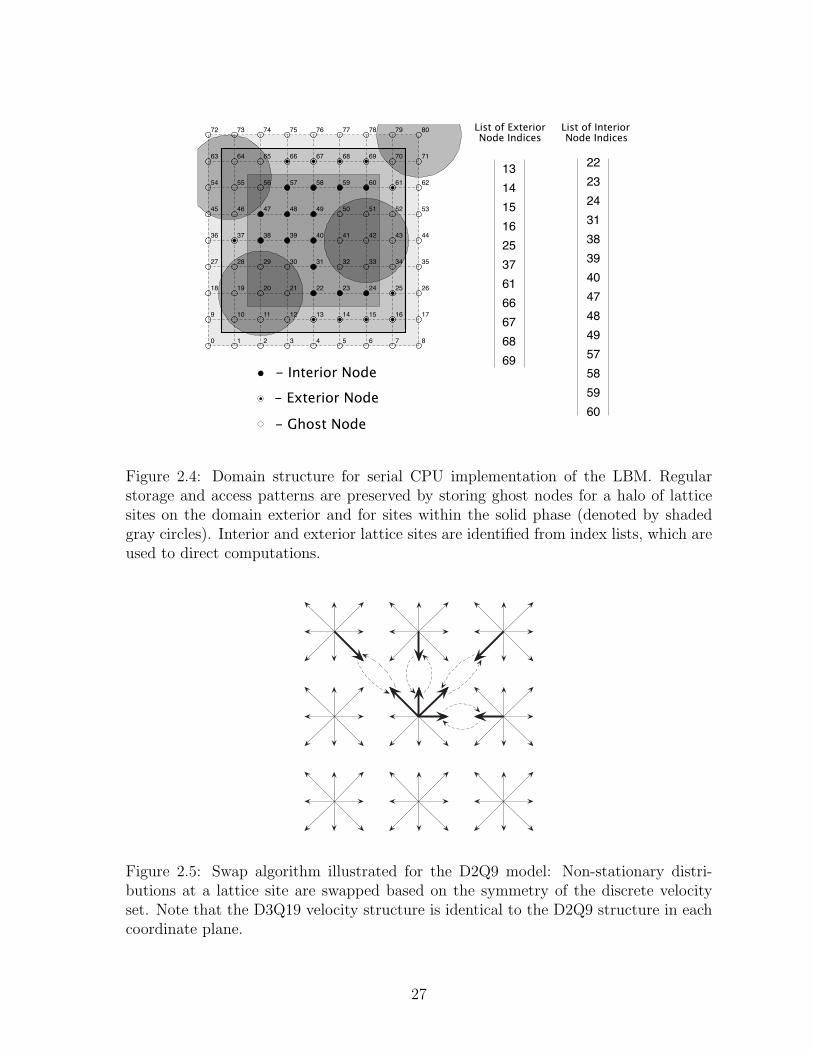
Figure 2.4: Domain structure for serial CPU implementation of the LBM. Regularstorage and access patterns are preserved by storing ghost nodes for a halo of latticesites on the domain exterior and for sites within the solid phase (denoted by shadedgray circles). Interior and exterior lattice sites are identified from index lists, which areused to direct computations.

Figure 2.5: Swap algorithm illustrated for the D2Q9 model: Non-stationary distri-butions at a lattice site are swapped based on the symmetry of the discrete velocityset. Note that the D3Q19 velocity structure is identical to the D2Q9 structure in eachcoordinate plane.

27

a particular lattice site will be stored in a contiguous block of memory. Alternative

data layouts can be constructed such that values needed to perform the streaming

step are stored sequentially, as well as hybrid layouts, which can demonstrate superior

performance for single component flows [116]. However, the collide layout is considered

here due to advantages for the Shan-Chen model, in which the distributions must be

accessed twice per iteration.

Due to memory bandwidth-limited performance of the LBM for most porous medium

applications, efficient implementation of the streaming step is critical to development of

fast LBM code since this step involves a large number of memory references. The swap

algorithm has been shown to achieve high lattice update rates while reducing storage

requirements relative to other approaches [117]. A schematic of the swap algorithm is

shown in Fig. (2.5). This approach makes use of the symmetry of the discrete velocity

set by noting that each discrete velocity ξq is associated with an opposing velocity

ξq = −ξq. At a particular lattice site xi, distribution fαq will translate to site xi + ξq,

and fαq (xi + ξq) will translate to site xi.

Memory bandwidth demands are significantly reduced by fusing the streaming step

with computations to the greatest extent possible. For the BGK and MRT methods,

the entire collision step can be carried out immediately after swapping the distributions

at a site provided that swapping has already been performed for all lattice sites xj :

j < i. For the multiphase Shan-Chen LBM, the non-local interaction force (Eq. (2.20))

must be fully implicit in terms of the fluid densities to ensure numerical stability. As a

consequence, the streaming and collision steps cannot be fused in any straightforward

way. Instead, density computations are fused with the streaming step, and all lattice

sites must be accessed subsequently in order to perform the collision step. This imposes

additional memory bandwidth demands for the multiphase Shan-Chen LBM relative

to single component methods, an important attribute that extends to other multiphase

schemes as well.

2.3.3 Parallel Implementation of the LBM (C++/MPI)

For parallel simulations using MPI, domain decomposition is necessary to distribute

computations between the processors. The method of orthogonal recursive bisection

(ORB), which was used in this work, has been shown to achieve excellent load balancing

for flow in porous medium systems while maintaining a small surface-to-volume ratio

to minimize communication expenses [140]. This approach recursively subdivides the

28

Pack send

buffer at

process p

Send data

from process p

to process r

Unpack

receive buffer

at process r

Prior to communication at process p After communication at process r

Figure 2.6: Schematic summarizing communication between processors p and r in aparallel LB simulation using MPI. Distributions needed by processor r are packed intoa send buffer on processor p. Using MPI, these values are provided to a receive bufferon processor r, from which they are unpacked to the proper location.

domain Ω to obtain subdomains Ω(p) for each processor p = 0, 1, . . . , Np − 1, where Np

is the total number of processors. Each subdomain is constructed in the same manner

as for the serial case, shown in Fig. (2.4). The index lists that store the interior and

exterior lattice sites for each processor p are denoted by X(p)int and X

(p)ext.

In parallel LBM’s implemented using MPI, computations are performed simultane-

ously for each subdomain. At the pre-processing stage, communication patterns are de-

termined based on the domain decomposition. Parallel implementation of the streaming

step requires communication to provide a subset of the distributions within the domain

exterior. To complete the streaming step at lattice site xi ∈ X(p)ext, processor r must

provide to processor p all distributions fαq (xi) that satisfy xi− ξq ∈ Ω(r),xi− ξq 6∈ Ωs.

The symmetry of the discrete velocity set ensures that each value received by processor

p from processor r will mirror a value sent by p to r. This eliminates the need to

store separate sets of indices for the distributions that each processor must send and

receive. Separate buffers are required to store the values sent and received as shown in

Fig. (2.6). Each processor maintains one buffer for distributions to send and one buffer

for distributions to receive. The total number of distributions sent to processor r by

processor p is N(p→r)f , which are offset from the beginning of the buffer by X

(p↔r)f . Due

to symmetry of the discrete velocity set, the number of values received by r from p is

N(p→r)f = N

(r←p)f .

For single-phase implementations, streaming is the only task that requires commu-

29

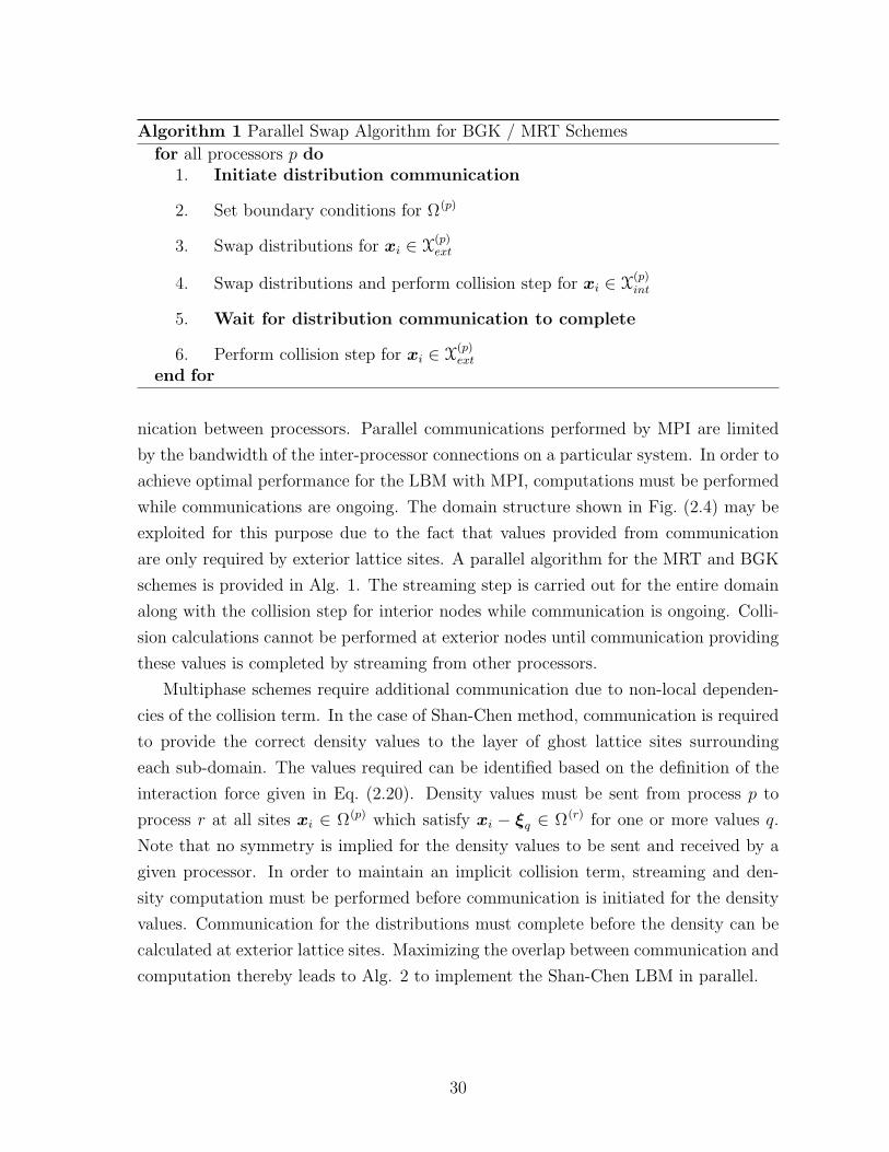
Algorithm 1 Parallel Swap Algorithm for BGK / MRT Schemes

for all processors p do1. Initiate distribution communication

2. Set boundary conditions for Ω(p)

3. Swap distributions for xi ∈ X(p)ext

4. Swap distributions and perform collision step for xi ∈ X(p)int

5. Wait for distribution communication to complete

6. Perform collision step for xi ∈ X(p)ext

end for

nication between processors. Parallel communications performed by MPI are limited

by the bandwidth of the inter-processor connections on a particular system. In order to

achieve optimal performance for the LBM with MPI, computations must be performed

while communications are ongoing. The domain structure shown in Fig. (2.4) may be

exploited for this purpose due to the fact that values provided from communication

are only required by exterior lattice sites. A parallel algorithm for the MRT and BGK

schemes is provided in Alg. 1. The streaming step is carried out for the entire domain

along with the collision step for interior nodes while communication is ongoing. Colli-

sion calculations cannot be performed at exterior nodes until communication providing

these values is completed by streaming from other processors.

Multiphase schemes require additional communication due to non-local dependen-

cies of the collision term. In the case of Shan-Chen method, communication is required

to provide the correct density values to the layer of ghost lattice sites surrounding

each sub-domain. The values required can be identified based on the definition of the

interaction force given in Eq. (2.20). Density values must be sent from process p to

process r at all sites xi ∈ Ω(p) which satisfy xi − ξq ∈ Ω(r) for one or more values q.

Note that no symmetry is implied for the density values to be sent and received by a

given processor. In order to maintain an implicit collision term, streaming and den-

sity computation must be performed before communication is initiated for the density

values. Communication for the distributions must complete before the density can be

calculated at exterior lattice sites. Maximizing the overlap between communication and

computation thereby leads to Alg. 2 to implement the Shan-Chen LBM in parallel.

30

Algorithm 2 Parallel Swap Algorithm for Shan-Chen Scheme

for All processors p do1. Initiate distribution communication

2. Set boundary conditions for Ω(p)

3. Swap distributions for xi ∈ X(p)ext

4. Swap distributions and compute density for xi ∈ X(p)int

5. Wait for distribution communication to complete

6. Compute density for xi ∈ X(p)ext

7. Initiate density communication

8. Perform collision step for xi ∈ X(p)int

9. Wait for density communication to complete

10. Perform collision step for xi ∈ X(p)ext

end for

2.3.4 Node-level Implementation of the LBM

Within a node, there is the possibility to take advantage of shared memory. However, for

LBM implementations this provides little advantage because the domain decomposition

has a relatively limited amount of data to be transferred between processors. Instead,

running an MPI process on each core of a node pins the domain to the directly attached

memory, and permits the communication of the halo nodes to proceed asynchronously

with the computation. It also greatly simplifies the software design to be able to use

MPI processes within nodes as well as across nodes. As a result of the aggregate memory

bandwidth limitations within a node, an LBM implementation may lose efficiency when

all cores are utilized. Thus maximum performance may be reached using less than the

total set of cores available at a node.

2.3.5 GPU Implementation of the LBM (CUDA)

Implementation of the LBM on a GPU represents a considerably different task from

a standard CPU implementation. Each GPU contains a large number of relatively

simplistic cores that are capable of carrying out tasks in parallel. Memory is allocated to

store data separately on both the CPU and GPU. Using syntax provided within CUDA,

31

blockIdx.x = 0

blockIdx.x = 1

blockIdx.x = 2

blockIdx.x = 3

Fluid Site

Solid Site

Figure 2.7: Domain decomposition for GPU implementation of the LBM. In this 2-Danalog, the 11 × 11 spatial domain is divided into grid blocks (nBlocks = 4) with afixed number of threads per threadblock (nThreads = 8). With nBlocks and nThreads

fixed, each thread performs computations for S = 4 lattice sites so that the entire spatialdomain is accounted for.

initialized variables are copied to the GPU where the main computations are performed.

When the simulation completes, data is copied back to the CPU so that it can be

output. CUDA kernels are based on a SIMD model in which many threads execute

identical instructions simultaneously. Domain decomposition on a GPU is structured

so as to take advantage of the multi-threaded framework, as shown in Fig. (2.7). The

number of threads nThreads and the number of threadblocks nBlocks can be varied

to maximize performance. Kernels provide instructions to the GPU that account for

all computations required to complete each iteration of the LBM. A set of registers

f0,f1,f2,...,f18 store the nineteen distributions required to perform computations

at each lattice site. These values reside in fast register memory once they have been

accessed from the main arrays. Computations are expressed in terms of these registers

in order to maximize performance.

The memory system of the GPU functions most efficiently when the values read

by each threadblock are aligned within contiguous blocks of memory. When data is

properly aligned, the GPU is able to coalesce memory accesses within each threadblock

into a smaller number of memory transactions. In order to use memory bandwidth most

efficiently, each half-warp of sixteen threads should access contiguous memory blocks

32

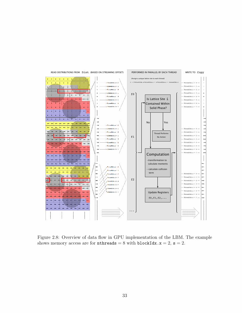
PERFORMED IN PARALLEL BY EACH THREADREAD DISTRIBUTIONS FROM (BASED ON STREAMING OFFSET)Dist WRITE TO Copy

ThreadIdx.x = 0

ThreadIdx.x = 1

ThreadIdx.x = 2

ThreadIdx.x = 3

ThreadIdx.x = 4

ThreadIdx.x = 5

ThreadIdx.x = 6

ThreadIdx.x = 7

f0

f1

f2

...

ThreadIdx.x = 0

ThreadIdx.x = 1

ThreadIdx.x = 2

ThreadIdx.x = 3

ThreadIdx.x = 4

ThreadIdx.x = 5

ThreadIdx.x = 6

ThreadIdx.x = 7

ThreadIdx.x = 0

ThreadIdx.x = 1

ThreadIdx.x = 2

ThreadIdx.x = 3

ThreadIdx.x = 4

ThreadIdx.x = 5

ThreadIdx.x = 6

ThreadIdx.x = 7

i = S*blockIdx.x*blockDim.x + s*blockDim.x + threadIdx.x

(Assign a unique lattice site to each thread)

No Yes

Thread Performs

No Action

Computation

- calculate collision term

calculate moments-transformation to

iIs Lattice Site Contained Within

Solid Phase?

f0,f1,f2,...

Update Registers

Figure 2.8: Overview of data flow in GPU implementation of the LBM. The exampleshows memory access are for nthreads = 8 with blockIdx.x = 2, s = 2.

33

of size 32, 64, or 128 bytes. In order to accomplish this, storage of the distributions is

dictated by the stream layout:

fαq (xi) = Distα[qN + i], (2.29)

for α ∈ E. For multi-component methods, separate distribution arrays are allocated

for each fluid component in order to reduce the number of registers needed to carry

out the computations. Note that this is in contrast to the storage scheme used for our

CPU implementation.

Since threadblocks do not execute in a predictable order, order-dependent streaming

algorithms such as the swap algorithm lose their advantage in GPU implementation.

In order to fuse the streaming step with computations on a GPU, it is necessary to use

a streaming algorithm that does not depend on the order the lattice sites are updated.

This means that the streaming and collision operations can not be fused for the swap

algorithm on a GPU, which therefore requires that GPU implementations have more

memory references than a corresponding CPU implementation.

Implementation of the streaming step using the two-lattice algorithm (TLA) is

schematically illustrated in Fig. (2.8). An additional copy of the distribution array,

labeled as Copy, is necessary to perform streaming with the TLA. The distributions

are read based on the streaming offset and stored in register memory for each thread.

Reading based on the streaming offset within a threadblock will access contiguous

blocks of memory for each distribution unless periodic boundary conditions shift one or

more distributions. High performance is contingent on a high number of computations

per memory operation. For the single component BGK and MRT schemes, the entire

collision process can be performed before writing the updated distributions back to

main memory. At even iterations, data is read and written as seen in Fig. (2.8). At

odd iterations, the position of Dist and Copy are interchanged.

For the multiphase Shan-Chen scheme, computation of density and velocity are

fused into the streaming step, and the distributions must be read into memory a second

time to perform the collision step. The distributions are therefore read one time based

on the streaming offset and once from the local indices, and written twice based on

the local indices. Good coalescence is ensured within a threadblock when reading

and writing is based on the local indices. In order to compute the interaction force,

18 additional density values must be accessed from memory for each component. As

a consequence, the Shan-Chen LBM must access approximately five times as many

34

variables for each iteration compared with single-component BGK and MRT LBM.

2.4 Results

We analyzed the performance of the BGK, MRT, and Shan-Chen LBM algorithms for

serial, parallel CPU, and GPU implementations. We also performed simulations for

realistic porous medium problems, a routine single-phase permeability calculation and

a more demanding Shan-Chen multiphase simulation of the drainage of a non-wetting

phase. These results are presented in turn in the sections that follow.

2.4.1 Serial CPU Implementation

BGKMRTShan-Chen

10 3 10 4 10 5 10 60

1

2

3

4

5

6

7

8

9

10

11

12

13

14

15Serial Performance of the LBM (Intel Xeon X5355)

Number of Nodes

MLU

PS

Figure 2.9: Serial performance for various implementations of the LBM as a functionof domain size. Once the lattice arrays exceed the L2 cache size, performance is limitedby available memory bandwidth.

Serial performance was analyzed for the BGK, MRT and Shan-Chen implementa-

tions of the LBM based on simulations performed using a single core of a 3 GHz Intel

Xeon X5355 processor. Lattice update rates are reported in million-lattice-updates-

per-second (MLUPS) as a function of lattice size in Fig. (2.9). In each case, cubic lat-

tices were considered. Results demonstrate that performance is roughly proportional

to the computational intensity of the model for domains that fit within the L2 cache

(2× 4 MB). This corresponds to a maximum lattice size of approximately 253 for the

35

Authors Year Processor GHz GB/s MLUPSWellein, Zeiser, Hager, 2006 Intel Xeon DP 3.4 5.3 4.8Donath AMD Opteron 1.8 5.3 2.7

Intel Itanium 2 1.4 6.4 7.6IBM Power4 1.7 9.1 5.9

Mattila, Hyvaluoma, Rossi, 2007 AMD Opteron 246 2.0 - 2.47Aspnas, WesterholmMattila, Hyvaluoma, 2008 AMD Opteron 2.0 - 4.02Timonen, Rossi Intel Xeon 3.2 - 4.67Heuveline, Krause, Latt 2009 AMD Opteron 2.6 6.4 1.9McClure, Prins, Miller - Intel Xeon 3.0 3.0 4.43

- Intel Nehalem 2.93 12.5 11.92

Table 2.1: Reported peak performance based on serial execution of the D3Q19 BGKLBM for a variety of processors [183, 117, 116, 77].

Model FLOPs Memory ReferencesBGK 295 19 read + 19 write = 38MRT 975 19 read + 19 write = 38Shan-Chen 2050 114 read + 78 write = 192

Table 2.2: Basic computational and memory reference parameters per lattice site forthe LBM models considered in this work.

36

BGK and MRT schemes, whereas the increased storage requirements of the Shan-Chen

scheme lead to a maximum of about 203. For flow in porous medium systems that are

representative of a macroscale representative elementary volume (REV) [17], the more

relevant performance estimates are those obtained for larger domain sizes. In these

cases, execution speed is primarily memory bandwidth limited with maximum execu-

tion speeds of 4.43 MLUPS for the BGK scheme, 3.55 MLUPS for the MRT scheme

and 1.25 MLUPS for the two-component Shan-Chen scheme. This memory bandwidth

limitation is key for the applications of greatest concern in porous medium science.

Performance of the BGK LBM is consistent with results reported by other authors

for the D3Q19 model, tabulated in Table 2.1 with hardware specifications noted when

available. Full periodic boundary conditions for the distributions and separate execu-

tion of interior and exterior lattice sites impose a slight performance penalty for our

implementation, both of which are necessary to carry out porous medium simulations

in parallel. Due to similar memory bandwidth demands, the MRT scheme achieves

similar performance to BGK model when the problem size exceeds the L2 cache limit.

The performance deficit for the MRT scheme indicates that computational intensity

does have limited impact on performance, meaning that memory bandwidth is not the

sole limiting factor. The performance of the Shan-Chen scheme is consistent with the

higher memory bandwidth demand associated with this model.

Total memory requirements are roughly equivalent for the BGK and MRT schemes

due to the fact that the distributions represent the only major variable that must be

allocated and stored. A total of 19×8 = 152 bytes are required to store the distributions

for a single component at a lattice site. An equivalent number of bytes must be accessed

from either data caches or main memory to perform each lattice update in the BGK and

MRT schemes. The demand for memory bandwidth is proportional to the number of

values which must be accessed from main memory. Due to the fusion of the streaming

and collision operations, the total number of memory references per lattice update is

given by Q(R+W ), where R denotes a memory read and W denotes a write. Memory

references for the single component D3Q19 BGK and MRT schemes are shown in Table

2.2, along with those for the two-component Shan-Chen scheme. In the Shan-Chen

LBM, arrays must be allocated to store both distribution and density values at each

lattice site for each of the two components, requiring 2× (19 + 1)× 8 = 320 bytes per

lattice site. Compared with the BGK and MRT schemes, significantly more memory

references are required for implementation of the Shan-Chen scheme. In addition to

the streaming requirement for two fluid components, additional memory references are

37

Topsail Franklin MMQNumber of cores per Node 8 4 32Total number of nodes 520 9,572 1Aggregate mem. bandwidth (GB/s) - 32 160Interconnect mem. bandwidth (GB/s) 1.0 1.6 -BGK (max. MLUPS/core) 5.31 5.04 11.92MRT (max. MLUPS/core) 3.78 3.71 5.67Shan-Chen (max. MLUPS/core) 1.06 0.998 2.237

Table 2.3: Overview of hardware specifications and LBM performance for the parallelsystems used in this work.

required to write the post-streaming density values and separately execute the collision

step. The total number of memory references for the Shan-Chen scheme are given by:

MRPLUS−C = (R +W )(Q×Nc)︸ ︷︷ ︸streaming

+W (Nc)︸ ︷︷ ︸density

+ (2R +W )(Q×Nc)︸ ︷︷ ︸collision

. (2.30)

Note that it is possible to implement each scheme with a greater number of memory

references but it is not possible to do so with less. For the two-component Shan-Chen

scheme, approximately five times as many values must be accessed from memory to

perform a lattice update compared with the basic MRT approach. Fig. (2.9) indicates a

roughly three-fold performance differential between these two methods, suggesting that

use of merged storage arrays combined with various compiler optimizations decreases

the relative cost of the Shan-Chen scheme.

2.4.2 MPI Implementation

Parallel performance tests were run on three different machines. Topsail is a Linux-

based supercomputing system with each compute node consisting of two quad-core 2.3

GHz Intel EMT processors with 2×4MB L2 Cache (ES5345) and 12 GB of memory.

Franklin is a Cray supercomputer with each compute node consisting of a 2.3 GHz

quad-core AMD Opteron (Budapest) processor with 8 GB of memory. MMQ is a four-

socket shared memory machine with a total of 32 Intel Nehalem cores, as illustrated

in Fig. (2.2). Additional specifications for these machines are provided in Table 2.3.

All scaling results are reported based on simulations performed for a porous medium

system generated from homogeneous sphere packings that approach the close-packing

density.

38

(a)

BGK (Franklin)BGK (Topsail)BGK (MMQ)MRT (Franklin)MRT (Topsail)MRT (MMQ)S-C (Franklin)S-C (Topsail)S-C (MMQ)

1 10 1000

0.1

0.2

0.3

0.4

0.5

0.6

0.7

0.8

0.9

1.0Parallel Scaling for the LBM

Number of Cores

Effic

ienc

y

Figure 2.10: Parallel efficiency based on a fixed problem size (2003) for various imple-mentations of the LBM on three supercomputing systems.

(a)

BGK (4M/core)BGK (250k/core)MRT (4M/core)MRT (250k/core)Shan-Chen (2M/core)Shan-Chen (250k/core)

1 10 1000

0.5

1

1.5

2

2.5

3

3.5

4

4.5

5

5.5

6

6.5

Scaling on Topsail

Number of Cores

MLU

PS /

Core

(b)

BGK (500k/core)BGK (125k/core)MRT (500k/core)MRT (125k/core)Shan-Chen (2M/core)Shan-Chen (250k/core)

1 10 1000

0.5

1

1.5

2

2.5

3

3.5

4

4.5

5Scaling on Franklin

Number of Cores

MLU

PS /

Core

Figure 2.11: Parallel efficiency based on constant sub-domain size per core for variousimplementations of the LBM on (a) Topsail (2 cores/node) and (b) Franklin.

39

Scaling behavior for a fixed lattice size (2003) is considered in Fig. (2.10). The

plots highlight the fact that memory bandwidth limited implementations tend to scale

poorly when adding additional cores on Xeon and Opteron CPU’s. This is a well

known consequence of the fact that memory bandwidth does not increase when adding

additional cores for these processors. The loss of efficiency is particularly severe on

topsail due to the larger number of cores per node and higher single-core performance

with lower aggregate memory bandwidth shared between the processor cores. Due to

the improved memory architecture of the Nehalem processor, implementations of the

LBM scale well across shared memory cores on MMQ. Scaling across nodes (Np > 8 on

Topsail, Np > 4 on Franklin) yields much better results than scaling across additional

cores on a node due to the fact that the available memory bandwidth increases with

the number of nodes. As the number of processor cores increases, communication

costs overwhelm computational costs and efficiency declines rapidly. This transition

will occur differently for different parallel systems based on the memory bandwidth for

communications.

While the efficiency exhibits a similar pattern for the BGK and MRT schemes, com-

munications drive down efficiency much sooner for the Shan-Chen scheme. This is easily

understood based on Algs. 1 and 2. For the single-component methods, communica-

tion for the distributions overlaps with interior streaming and collision computations,

which make up the majority of the computational expenditure. For the Shan-Chen

LBM, communication for the distributions overlap with less demanding computations

since collision cannot be performed. Communication required to provide density values

represents an additional bottleneck.

The plots provided by Fig. (2.10) can be used to determine the minimum subdo-

main size per core before communication becomes the dominant performance bottle-

neck. Since the communication-to-computation ratio can be approximated by a surface

area-to-volume ratio, maintaining sufficiently large sub-domains Ω(p) ensures that com-

munication will not limit efficiency. The LBM can be scaled to run on a very large

number number of cores by increasing the total domain size with the number of cores.

The minimum sub-domain sizes are approximately 503 for the BGK/MRT schemes

and 643 for the Shan-Chen scheme. Maximum sub-domain sizes are determined by the

amount of memory available on each node. Efficiency (scaled by MLUPS/core) is shown

in Fig. (2.11). These results demonstrate that even for massively parallel simulations,

each core is capable of sustaining a relatively constant number of MLUPS on par with

the performance obtained for the serial case provided that subdomains are sufficiently

40

large.

Maximum performance for a domain of size 6353 using 512 cores on Franklin was

2177.5 MLUPS for BGK, 1715.2 MLUPS for MRT, and 435.2 MLUPS for Shan-Chen.

On Topsail, for a domain of size 8003 simulation using 128 cores produced a maximum

performance of 862.7 MLUPS and 485.1 MLUPS for the BGK and MRT schemes,

respectively. For Shan-Chen LBM, peak performance was 157.44 MLUPS based on

a lattice size of 6353 distributed across 128 cores. On MMQ, the peak performance

on sixteen cores was 170.4 MLUPS for the BGK model, 87.3 MLUPS for the MRT

model and 32.8 MLUPS for Shan-Chen. The advantages of the modern setup shown in

Fig. (2.2) include a nearly two-fold performance increase in per-core performance with

excellent scaling achieved in shared memory. This level of performance is expected to

scale equally well in a distributed memory setting.

2.4.3 GPU implementation

(a)

BGKMRTShan-Chen

10 4 10 5 10 60

20

40

60

80

100

120

140

160

LBM Performance on GPU

Number of Nodes

MLU

PS

Figure 2.12: Performance on NVidia QuadroPlex Model IV Quadro FX 5600 for arange of problem sizes using implementations of the BGK, MRT and Shan-Chen LBM.

Simulations were carried out using a NVidia QuadroPlex Model IV Quadro FX5600

graphics card with 1.5 GB RAM. Limitations of this hardware restrict calculations to

single-precision floating point. By varying the number of threads and threadblocks, op-

timal performance was obtained by choosing nBlocks = 32 and nThreads = 128. While

the FX5600 is theoretically capable of accommodating up to 512 threads, there is insuf-

ficient register memory to perform calculations for the D3Q19 LBM with nThreads >

128. Domain sizes were varied from 163–2083 for the BGK and MRT schemes, and

41

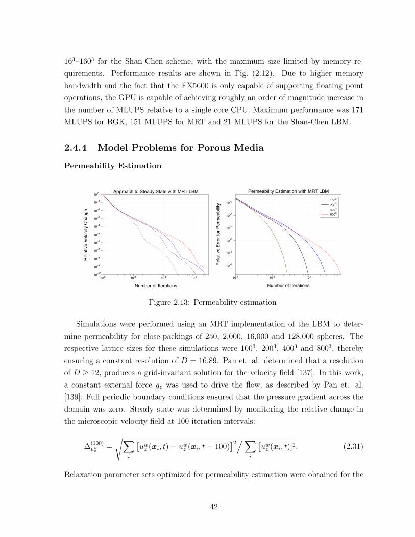
163–1603 for the Shan-Chen scheme, with the maximum size limited by memory re-

quirements. Performance results are shown in Fig. (2.12). Due to higher memory

bandwidth and the fact that the FX5600 is only capable of supporting floating point

operations, the GPU is capable of achieving roughly an order of magnitude increase in

the number of MLUPS relative to a single core CPU. Maximum performance was 171

MLUPS for BGK, 151 MLUPS for MRT and 21 MLUPS for the Shan-Chen LBM.

2.4.4 Model Problems for Porous Media

Permeability Estimation

10 2 10 3 10 4 10 510 -10

10 -9

10 -8

10 -7

10 -6

10 -5

10 -4

10 -3

10 -2

10 -1

10 0 Approach to Steady State with MRT LBM

Number of Iterations

Rela

tive

Velo

city

Chan

ge

1003

2003

4003

8003

10 2 10 3 10 4

10 -7

10 -6

10 -5

10 -4

10 -3

10 -2

Permeability Estimation with MRT LBM

Number of Iterations

Rela

tive

Erro

r for

Per

mea

bility

Figure 2.13: Permeability estimation

Simulations were performed using an MRT implementation of the LBM to deter-

mine permeability for close-packings of 250, 2,000, 16,000 and 128,000 spheres. The

respective lattice sizes for these simulations were 1003, 2003, 4003 and 8003, thereby

ensuring a constant resolution of D = 16.89. Pan et. al. determined that a resolution

of D ≥ 12, produces a grid-invariant solution for the velocity field [137]. In this work,

a constant external force gz was used to drive the flow, as described by Pan et. al.

[139]. Full periodic boundary conditions ensured that the pressure gradient across the

domain was zero. Steady state was determined by monitoring the relative change in

the microscopic velocity field at 100-iteration intervals:

∆(100)uw

z=

√∑i

[uwz (xi, t)− uwz (xi, t− 100)

]2/∑i

[uwz (xi, t)]2. (2.31)

Relaxation parameter sets optimized for permeability estimation were obtained for the

42

MRT LBM based on the work of d’Humieres et. al. [44]. Permeability estimates were

not obtained for the BGK LBM due to the well-known deficiencies of this approach

[139].

Two aspects of the approach to steady state are shown in Fig. (2.13). In Fig. (2.13)

(a), the magnitude of changes to the microscopic velocity field as measured by Eq. (2.31)

are plotted as a function of simulation time. The initial response of the system is

largely independent of the domain size due to the acceleration of the velocity field from

a uniform zero state. At longer simulation times, the number iterations required to

reduce the error is a function of domain size. Permeability estimates computed from

the microscopic velocity field every 100 iterations were compared to the permeability

obtained from the final velocity field in order to estimate the error, which is plotted in

Fig. (2.13) (b). The macroscale permeability was observed to converge more rapidly

than the microscale velocity field, which is not surprising given the averaged nature of

the macroscale variable. Such calculations are considered routine and representative

values for media of the nature used in this work can be obtained for domains on the scale

of 2003. Given the lattice update rates previously computed, it is straightforward to

show that such computations can easily be done at the REV scale on a single processor

in a manageable time.

Drainage Simulation

D=20.27D=16.89D=13.51

0.2 0.3 0.4 0.5 0.6 0.7 0.8 0.90

0.2

0.4

0.6

0.8

1.0

1.2

1.4

1.6

1.8

2.0

2.2Resolution Dependence of the Shan-Chen LBM

sw

p c D

Figure 2.14: Resolution dependence for wetting-phase drainage curve based on simula-tions performed in a packing of 250 equally sized spheres.

Resolution dependence for drainage simulations performed in a packing of 250

equally sized spheres is shown in Fig. (2.14). Lattice sizes were 803, 1003 and 1203 for

43

resolutions of D = 13.51, 16.89 and 20.27, respectively. Pressure boundary conditions

were implemented in order to match a typical experimental setup [200]. The domain

was initially saturated with wetting-phase and drained by incrementally increasing the

pressure difference pc. For each point the inlet densities were chosen according to

ρn = 1.0 + 32pc, ρ

w = 0.0 and the outlet densities are ρn = 0.0, ρw = 1.0 − 32pc. The

sequence of pressure differences was chosen such that the sequence of values pcD remain

constant at all resolutions.

In order to obtain valid equilibrium relationships, fluids must be permitted to equi-

librate fully. Various criteria have been used to monitor equilibration of the Shan-Chen

LBM. Pan et. al. computed the capillary number, which is problematic due to spurious

velocities near interfaces [138]. A saturation-based termination criteria has also been

applied [148]. In this work, we evaluated equilibration based on the density fluctuation,

defined by:

∆(1k)ρ =

√∑i

∑α

[ρα(xi, t)− ρα(xi, t− 1000)

]2/∑i

∑α

[ρα(xi, t)

]2. (2.32)

The density fluctuation accounts for both local changes in density values due to the

equilibration of the pressure and interface shape in addition to macroscopic fluid flow.

Various factors influence the resolution-dependence of Shan-Chen based equilibria.

Since the equilibration of multiphase porous medium systems is typically dominated

by interfacial physics, local equilibria are extremely sensitive to small changes in solid

boundary locations, which is manifested in the sensitivity of pc − sw curves to changes

in resolution. Establishing grid independence for the Shan-Chen method is complicated

by the fact that maintaining immiscibility and numerical stability limit the parameters

Gwn and Gs to within a relatively narrow range. As a result, surface tension cannot be

maintained as a constant between simulations performed over a wide range of resolu-

tions. For our simulations, the interaction parameters were Gwn = 0.09 and Gs = 0.01.

Due to proportionality between pressure and density, the density ratio of the two fluids

changes for each point on the capillary pressure-saturation curve. Coarser resolutions

require larger density differences, suggesting that the shifting density ratio may bias

curves obtained for coarsely resolved systems. Although reasonable qualitative agree-

ment in curve shape is observed at D = 16.89, it is clear that higher resolutions are

needed to obtain a grid-independent value for each point on the curve.

The approach to the equilibrium state is shown for D = 16.89 in Fig. (2.15) (a)

and (b). Of principle concern is the length of time required for the saturation to stabi-

44

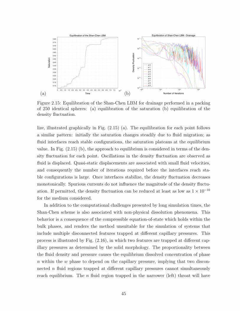
(a)10 60 0.5 1.0 1.5 2.0 2.5 3.0 3.5 4.0 4.5 5.0 5.5 6.0 6.5 7.0 7.5

0.10

0.15

0.20

0.25

0.30

0.35

0.40

0.45

0.50

0.55

0.60

0.65

0.70

0.75

0.80

Equilibration of the Shan-Chen LBM

Time

Satu

ratio

n

(b)

pt 0pt 1pt 2pt 3pt 4pt 5pt 6pt 7pt 8pt 9

10 3 10 4 10 5 10 610 -6

10 -5

10 -4

10 -3

10 -2

10 -1

Equilibration of Shan-Chen LBM - Drainage

Number of Iterations

Dens

ity F

luct

uatio

n

Figure 2.15: Equilibration of the Shan-Chen LBM for drainage performed in a packingof 250 identical spheres: (a) equilibration of the saturation (b) equilibration of thedensity fluctuation.

lize, illustrated graphically in Fig. (2.15) (a). The equilibration for each point follows

a similar pattern: initially the saturation changes steadily due to fluid migration; as

fluid interfaces reach stable configurations, the saturation plateaus at the equilibrium

value. In Fig. (2.15) (b), the approach to equilibrium is considered in terms of the den-

sity fluctuation for each point. Oscillations in the density fluctuation are observed as

fluid is displaced. Quasi-static displacements are associated with small fluid velocities,

and consequently the number of iterations required before the interfaces reach sta-

ble configurations is large. Once interfaces stabilize, the density fluctuation decreases

monotonically. Spurious currents do not influence the magnitude of the density fluctu-

ation. If permitted, the density fluctuation can be reduced at least as low as 1× 10−10

for the medium considered.

In addition to the computational challenges presented by long simulation times, the

Shan-Chen scheme is also associated with non-physical dissolution phenomena. This

behavior is a consequence of the compressible equation-of-state which holds within the

bulk phases, and renders the method unsuitable for the simulation of systems that

include multiple disconnected features trapped at different capillary pressures. This

process is illustrated by Fig. (2.16), in which two features are trapped at different cap-

illary pressures as determined by the solid morphology. The proportionality between

the fluid density and pressure causes the equilibrium dissolved concentration of phase

n within the w phase to depend on the capillary pressure, implying that two discon-

nected n fluid regions trapped at different capillary pressures cannot simultaneously

reach equilibrium. The n fluid region trapped in the narrower (left) throat will have

45

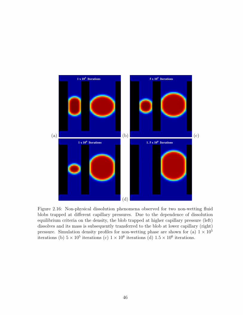
(a)

1 x 105 Iterations

(b)

5 x 105 Iterations

(c)

1 x 106 Iterations

(d)

1. 5 x 106 Iterations

Figure 2.16: Non-physical dissolution phenomena observed for two non-wetting fluidblobs trapped at different capillary pressures. Due to the dependence of dissolutionequilibrium criteria on the density, the blob trapped at higher capillary pressure (left)dissolves and its mass is subsequently transferred to the blob at lower capillary (right)pressure. Simulation density profiles for non-wetting phase are shown for (a) 1 × 105

iterations (b) 5× 105 iterations (c) 1× 106 iterations (d) 1.5× 106 iterations.

46

a higher capillary pressure, higher density, and higher solubility compared with the

blob trapped at lower capillary pressure. This leads to non-physical mass transfer from

blobs trapped at higher capillary pressure to those trapped at lower capillary pressure.

Ultimately, this dissolution process will continue until only one blob remains. For sim-

ulations carried out with pressure boundary conditions, the existence of disconnected

phases is precluded at equilibrium, and only n-phase connected to the reservoir can

remain at equilibrium. This phenomena explains the apparent absence of disconnected

phases from the simulations reported by Porter et. al. [148]. The existence of dis-

connected phases observed by Pan et. al. is due to termination prior to equilibrium

as a consequence of the termination criteria used [138]. Several alternative multiphase

formulations exist which may provide a more appropriate description of disconnected

features, but these methods have not yet been applied in a porous medium setting

[85, 101, 122, 97].

2.5 Discussion

Typical simulation scenarios for the LBM in porous medium systems are limited either

by total simulation time or by the amount of memory required to store the lattices. The

latter case is exemplified by permeability calculation, in which very large lattices sizes

may be considered due to the relatively small number of iterations needed to obtain

a steady state solution for the velocity field. The maximum domain size considered

in this work contained 128,000 equally-sized spheres, leading to a simulation domain

consisting of 8003 lattice nodes. For this case, 80, 000 iterations of the MRT LBM

produce a permeability estimates accurate to seven significant figures. These results

can be achieved without any loss of efficiency due to the fact that excellent scaling can

be achieved for MPI implementations as long as sufficiently large sub-domains (> 503)

are maintained for each processor core. For the MRT LBM, the lattice update rate

can be maintained at 3.0–3.5 MLUPS per processor core even in massively parallel

simulation. The primary performance drop-off is due to adding additional cores of

a multi-core CPU, a well known limitation that can be alleviated by using improved

hardware such as the intel Nehalem processor, which demonstrates excellent scaling

across shared memory cores.

Multiphase drainage simulations performed using the Shan-Chen method highlight

challenging computational realities for simulating multiphase flows in porous media.

High resolution is necessary for grid-independent results, and the number of iterations

47

required to allow the system to equilibrate are several orders of magnitude higher than

for the single-phase case. The primary reason for this difference is that the convergence

to steady state is limited by the mach number in single-phase simulations, whereas mul-

tiphase simulations achieve steady state only after rearrangements of fluid interfaces,

a process which is limited by the typically small flow velocity. While the Shan-Chen

LBM is demonstrated to scale to 1.0 MLUPS per processor core as long as subdomain

sizes are larger than 643, total simulation time severely restricts the maximum domain

size that can be considered. These results highlight the potential importance of algo-

rithm optimizations that reduce the number of lattice updates required per-iteration

for multiphase LBM. Sophisticated algorithms that utilize local grid refinement in the

vicinity of interfaces and/or permit larger time steps have the potential to address

this issue directly and significantly reduce the computational burden associated with

multiphase simulation. It is also pointed out that non-physical behavior makes the

Shan-Chen LBM ill-suited for simulation of porous medium systems. It is likely that

more computationally intensive methods would be necessary to properly describe fluid

physics, thereby increasing the computational burden associated with solution of this

problem.

The capability for GPU’s to accelerate the LBM is most evident for the case of single-

phase flow, for which the memory accesses can be effectively hidden by computations.

Relative speedup is less dramatic for the two-component Shan-Chen scheme, an effect

which is attributed to the fact that fusion of the streaming and collision cannot be

achieved and twice as many memory references must be performed during the collision

step in order to incorporate the interaction forces. While the GPU speedup relative

to serial CPU implementation is significant for all schemes considered, higher lattice

update rates can still be achieved via MPI implementation utilizing many CPU cores.

Since distributed memory parallelization is necessary to achieve large domain sizes,

MPI implementations utilizing many GPU’s across multiple nodes would be necessary

to perform most porous medium simulations.

While the use of GPU’s to accelerate the LBM is attractive, memory system im-

provements to CPU’s such as those implemented in the Nehalem processor lead to

similar performance for typical configurations. For more complex problems such as

multiphase simulation, sophisticated flow control and pre-fetching allow CPU’s to out-

perform GPU’s when scaling across nodes. Using 8 cores of the Nehalem processor

produced a lattice update rate of 17.44 for double precision floating point calculations,

whereas the GPU achieved only a slightly higher lattice update rate for a less inten-

48

sive single precision calculation. The implications for more sophisticated multiphase

schemes, which require significantly more memory references in the interfacial force

computation, may further disadvantage GPU implementations in this respect.

2.6 Conclusions

1. Performance of the LBM is dominated by the number of memory references re-

quired by the scheme.

2. Performance of the LBM on a CPU core is sensitive to the choice of data structures

and access patterns. Optimization strategies addressing these considerations are

mature and extensible to a wide range of schemes. While streaming step opti-

mization is the primary focus for single component schemes, multi-component

schemes introduce significantly more memory references and impose additional

algorithmic constraints.

3. Implementation of the LBM on a GPU can be associated with a significant

speedup relative to serial CPU approaches due to the higher memory bandwidth

of the GPU. The speedup associated with the multiphase Shan-Chen LBM is less

dramatic than for the single component approaches, an effect that is attributed

to advantages gained from sophisticated compiler optimizations that bolster the

CPU performance for this scheme. The multi-core performance of the Nehalem

processor is competitive with that of the GPU and considerably better than for

the previous generation of CPU’s.

4. Permeability estimates can be reliably obtained for very large porous medium

systems due to rapid convergence to steady state and excellent scaling for large

domain sizes on distributed memory supercomputers.

5. Simulation of multiphase porous medium flows are constrained by significant chal-

lenges that cannot be overcome based on existing hardware, algorithms, and opti-

mization strategies. While good scaling can be achieved for the multi-component

Shan-Chen LBM, long equilibration times severely limit simulation sizes. This

result underscores the importance associated with development of schemes that

utilize adaptive grid refinement and allow larger time steps, thereby reducing the

number of lattice updates required to reach steady state solutions.

49

6. New multiphase porous medium LBM algorithms will be needed to resolve the im-

portant problem of two-fluid-phase flow and quasi-static distributions for systems

that contain disconnected non-wetting phases.

50

Chapter 3

Morphological Tools

3.1 Approximation of Interfacial Properties in Mul-

tiphase Porous Medium Systems

3.1.1 Introduction

The standard continuum approach for modeling multiphase flow in porous medium

systems avoids explicit description of complex microscopic phenomena by making use

of closure relations that do not rigorously incorporate microscale physics. For exam-

ple, commonly used closure relations state a functional dependence between capillary

pressure and fluid saturation [176, 27] that depend upon the system history due to

non-wetting phase entrapment and other pore-scale effects. It has been posited that

the specification of additional variables, including specific interfacial areas, common

curve lengths and interfacial curvatures, may reduce or eliminate the hysteresis ob-

served in traditional closure relations [57]. Pore-scale, or microscale, investigations of

this hypothesis have been undertaken using network models [32, 75] and experimental

approaches using two-dimensional micro-models [35].

In addition to evidence that specification of interfacial areas is necessary to deter-

mine the thermodynamic state of a multiphase system, interfaces also play an important

role in other processes. In porous medium systems, interfaces must be taken into ac-

count in order to rigorously develop equations for conservation of mass, momentum, and

energy [57]. Furthermore, because interphase mass exchange takes place at interfaces,

interfacial areas are also important to the modeling of processes such as dissolution and

sorption [125, 90]. For these reasons, resolving the role of interfacial areas is an essential

step in the development of multiphase porous medium models that rigorously connect

microscale characteristics to macroscale models. Interfacial curvatures and common

curve lengths are also of interest in evolving theories [57], and these quantities have

received little attention in the porous medium literature.

The nature of porous media typically makes simulation as well as direct measure-

ment of microscale quantities difficult. As a consequence, many of the methods that

have been used to estimate interfacial areas rely upon assumptions that are not ideal;

and it is often difficult to assess the magnitude of errors that result. These meth-

ods include theoretical approaches to compute interfacial areas based upon capillary

pressure-fluid saturation relations using thermodynamic principles in conjunction with

assumptions about the geometry of the entrapped fluid [25, 136]. Interfacial areas have

also been estimated with pore-network models, in which fluid flow is simulated through

porous media constructed using idealized pore geometries, such as spherical pore bodies

connected by cylindrical throats, and certain other simplifying assumptions. Because of

the simplified geometry, interfacial areas and common curve lengths can be computed

easily in network models [46, 20, 55]. Although such models do provide a window

into pore-scale phenomena, simplifications employed can contribute to deviations in

the behavior of ideal systems compared to the real system of concern.

In cases where interfacial areas have been measured experimentally, techniques uti-

lizing interfacial tracers, such as surfactants, have been the predominant approach

[158, 160, 5, 157, 94]. Recently, Cheng et. al. [35] synthesized two-dimensional porous

medium networks, which allowed them to examine the interfaces for a two-fluid-phase

system. Magnetic resonance imaging has been used to resolve interfaces in three-

dimensional multiphase systems [90]. X-ray computed micro-tomorgraphy has also

been used to obtain high resolution images of porous media and interfacial areas [38].

In each of these instances, it was implied that the marching cubes (MC) algorithm was

used to compute the interfacial area, but no discussion of numerical error was presented.

Other authors have experienced difficulty achieving accurate area estimates when using

the MC algorithm for porous medium work [40]. In order to develop constitutive rela-

tions that can be used in predictive models, it is necessary to extract accurate estimates

of interfacial areas and related quantities.

Numerical simulation of fluid flows through realistic porous media presents an at-

tractive opportunity to study details of multiphase flow at the microscale. Sophisticated

methods such as the lattice Boltzmann (LB) method are capable of recovering hysteretic

behavior observed in experimental systems [141]. Because LB methods do not typically

track the interface between fluids, these interfaces must be extracted afterwards. Meth-

52

ods to estimate interfacial properties have not yet been advanced specifically to deal

with the nuances of such microscale simulations, which in principle offer challenges and

opportunities beyond those of simplified network models.

The overall goal of this work is to develop computational tools needed to approx-

imate accurately interfaces, common curves, and interfacial curvatures for two-fluid-

phase porous medium systems. The specific objectives of this work are: (1) to develop

methods that improve the estimation of interfacial quantities in multiphase porous

medium systems compared to MC methods currently in use; (2) to develop algorithms

showing the implementation of these methods; (3) to advance an approach to approxi-

mate interfacial quantities resulting from LB simulation of multiphase porous medium

systems; (4) to assess the accuracy of the methods developed compared to extant ap-

proaches; and (5) to consider ways in which interfacial property estimations can be

further improved.

3.2 Methods

The MC algorithm was originally designed as a tool to construct surfaces of constant

density from three-dimensional medical datasets [108]. Subsequently, a number of au-

thors proposed improvements to the original algorithm to overcome shortcomings and

improve efficiency [156, 43, 199]. Although the MC algorithm has been used to com-

pute interfacial areas in porous medium systems, the resulting estimates have not been

particularly accurate [40]. We seek to improve and extend these results for a range of

multiphase porous medium systems.

We consider a regularly shaped domain Ω ⊂ Re3, such as a cube or rectangular

prism, with a boundary Γ. The external closure of the domain is given as Ω = Ω ∪ Γ.

The domain is comprised of up to three phases such that Ω = Ωw ∪ Ωn ∪ Ωs, where

the subscripts w, n, and s specify a wetting fluid phase, a non-wetting fluid phase, and

a solid phase. Consider a general set of phase qualifiers, which we denote using the

subscripts α, β, and γ, where it is assumed that α 6= β 6= γ. For a given phase α, the

closure of the domain is Ωα = Ωα∪Γα, where Γα = Γαi∪Γαe, the subscript i denotes an

internal boundary, and the subscript e denotes an exernal boundary, such that Γαe ⊂ Γ

and Γαi =⋃β 6=α(Ωα ∩ Ωβ) 6⊂ Γ.

The goal of this work is to identify and measure two types of entities, interfacial

areas, which we define as Ωαβ = Ωα ∩ Ωβ ⊂ Re2; and common curves, which we define

as Ωαβγ = Ωα ∩ Ωβ ∩ Ωγ ⊂ Re1. The extent of Ω has a measure of volume V , Ωα

53

has a measure of volume V α, Ωαβ has a measure of area Aαβ, and Ωαβγ has a measure

of length Lαβγ. Specific measures are often of interest for macroscale porous medium

systems and are described as the volume fraction εα = V α/V , the specific interfacial

area εαβ = Aαβ/V , and the specific common curve length εαβγ = Lαβγ/V . Quantities

such as the mean microscale curvature Jαβ of Ωαβ and the macroscale counterpart Jαβ

are also of interest. More complete definitions of systems, entities, and scales relevant

to the multiphase systems of concern in this work are available in the literature [127].

The methods developed in this work provide approximations for these macroscale

geometric quantities and a basis upon which graphical reconstruction may be based.

In the sections that follow, we summarize the MC approach, a porous media marching

cubes (PMMC) approach, a higher order porous media marching cubes (HOPMMC)

approach, approximation of curvatures, and data source issues.

3.2.1 Marching cubes algorithm

The MC algorithm is a procedure that may be used to construct an approximation of

Ωαβ, which we will refer to as Ωαβ. This reconstructed surface may be used for some

combination of graphical visualization and estimation of the extent, say Aαβ or εαβ,

and other properties. This construction requires two components: a discretization of

Ω, and a general function containing information related to the distribution of phases

G(x) defined, at least approximately as G(x), ∀x ∈ Ω. These two components will be

summarized in turn.

Consider a domain aligned with a Cartesian coordinate system Ω = [0, `]× [0, `]×[0, `] ⊂ Re3 of length ` on each side discretized with a mesh Mh consisting of n

evenly spaced nodes along each side of the domain for a total of n3 nodes. The node

spacing is h = `/(n− 1) = ∆x = ∆y = ∆z. Mh can be used to describe a set of cubes

C = Ωl|l = 1, . . . , n3c, where Ωl = [(i−1)∆x, i∆x]×[(j−1)∆y, j∆y]×[(k−1)∆z, k∆z],

nc = n − 1, and l = i + (j − 1)nc + (k − 1)n2c and i, j, and k refer to integer indexes

to a cube location defined by eight bounding nodes inMh in the x, y, and z Cartesian

coordinate direction, respectively. Each cube Ωl has boundary Γl, which contains a set

of 12 edges Ec,l = eli, i = 1, . . . 12 that are each parallel with one of the coordinate

directions and connect a pair of the eight nodes from Mh that together bound cube

Ωl. The set of nodes comprising the end points of the i edge in Ωl are denoted Nli =

nli1, nli2, the set of nodes bounding Ωl are denoted Nc,l =⋃i=1,··· ,12 Nli, and the set of

spatial locations corresponding to these boundings nodes are Xl = xi, i = 1, · · · , 8.

54

The set of all nodes in Mh are defined as N = ni, i = 1, ..., n3.G(x) represents a general function containing information related to the distribution

of phases. Because many different approaches exist to measure and represent phase

distributions in a multiphase system, the specific nature of this function will depend

upon details of the application. For the time being, we will assume G(x) is a continuous,

smooth, real-valued function that may be evaluated at all nodes in Mh. We will

furthermore assume that a value ν is known such that G(x) = ν for x ∈ Ωαβ. Thus the

approximation of Ωαβ reduces to approximating the surface where G(x) = ν, which is

accomplished using linear interpolation along the set of edges Ec,l within each Ωl using

values of G(x) at the eight nodes from Mh that bound Ωl and form the members of

the end-point nodal sets Nli.

Consider the location of two end points of any edge to be x− and x+ and the

corresponding general distribution function values corresponding to these end points to

be G(x−) and G(x+). A vertex where G(x) = ν will exist along the edge if and only if

[G(x+)− ν][G(x−)− ν] ≤ 0 (3.1)

If a vertex exists along the edge, the location of the vertex may be approximated using

linear interpolation as

xv = x+ +G(x+)− ν

G(x+)−G(x−)(x− − x+) (3.2)

Evaluating Eqs. (3.1) and (3.2) for each edge in a cube, and eliminating duplicates

that fall at nodes, will lead to a set of vertices Vαβ,l such that the number of members

in the set is bounded by 0 ≤ Card (Vαβ,l) ≤ 12. A non-unique set of triangles Tαβ,l

can be constructed from the set of Vαβ,l where Card (Tαβ,l) = max[0,Card (Vαβ,l)− 2].

To preserve continuity, if multiple vertices exist for a face of a cube, they should be

connected identically for both cubes bounded by the face. Global sets of vertices Vαβ

and triangles Tαβ can be constructed by concatenating all unique entries in all local cube

sets Vαβ,l and Tαβ,l, respectively. The global sets can be used for graphical purposes,

and estimation of various measures of the system.

To aid clarity, we illustrate the MC algorithm for a two-dimensional system in

Fig. 3.1. In this figure, the shading indicates the value of G(x) and the surface of

interest is located at G(x) = 0.5. The white square indicates an example local cell and

two vertices exist in this cell, which follows from examination of the values at the nodes

55

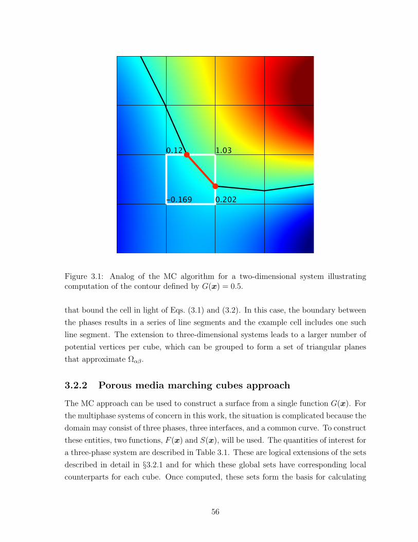
-0.169 0.202

0.12 1.03

Figure 3.1: Analog of the MC algorithm for a two-dimensional system illustratingcomputation of the contour defined by G(x) = 0.5.

that bound the cell in light of Eqs. (3.1) and (3.2). In this case, the boundary between

the phases results in a series of line segments and the example cell includes one such

line segment. The extension to three-dimensional systems leads to a larger number of

potential vertices per cube, which can be grouped to form a set of triangular planes

that approximate Ωαβ.

3.2.2 Porous media marching cubes approach

The MC approach can be used to construct a surface from a single function G(x). For

the multiphase systems of concern in this work, the situation is complicated because the

domain may consist of three phases, three interfaces, and a common curve. To construct

these entities, two functions, F (x) and S(x), will be used. The quantities of interest for

a three-phase system are described in Table 3.1. These are logical extensions of the sets

described in detail in §3.2.1 and for which these global sets have corresponding local

counterparts for each cube. Once computed, these sets form the basis for calculating

56

interfacial areas, common curve lengths, and other quantities of interest. Computing

the members of these sets depends upon the nature of the data available, the smoothness

of this data, the fraction of the domain over which each source of data is well-defined,

and modifications made to the basic MC algorithm.

Table 3.1: Sets needed for the PMMC algorithm.Set Description

Nc,l,Nli,Ec,l,Xl nodes bounding cube, nodes forming all edges i, edges in cube l, andlocations of nodes bounding cube

Vwn,Vns,Vws,Vs vertices on the respective surfaceTwn,Tns,Tws,Ts triangles comprised of vertices on the respective surfaceVwns vertices where the three phases meetLwns line segments consisting of pairs of vertices from Vwns

Consider the common case of a three-phase system in which a smooth, continu-

ous, differentiable function related to the location of the solid phase S(x) is defined

∀x ∈ Ω. Also, a second smooth, continuous, differentiable function related to fluid

properties F (x) is defined ∀x ∈ Ω. Such functions can result from either experimen-

tal measurements or computational approaches applied to three-phase porous medium

systems. The surface of the solid phase corresponds to S(x) = νs, and Ωwn corresponds

to F (x) = νwn. In some cases, it may be true that F (x) is only defined ∀x ∈ Ωw ∪Ωn.

An example of this would be if F (x) corresponds to the fluid density. Our PMMC

algorithm is designed to construct the objects of interest for either of these cases.

The sets listed in Table 3.1 are constructed locally in each cube using Algorithm 3.

For each cube, local sets corresponding to nodes, edges, and the corresponding spatial

locations are formed. One of five conditions must hold for each cube given the values of

S(x) and F (x) at the nodes in the cube: (1) all nodes have values that correspond to a

single phase Ωα, thus no interfaces or common curve segments exist; (2) all of the nodes

are in a fluid phase with some values of F (x) ≤ νwn and some value of F (x) > νwn,

thus only the Ωwn interface exists; (3) some of the nodes have S(x) ≤ νs and are in Ωs,

and the rest of the nodes have F (x) ≤ νwn and are in Ωw, thus only the Ωws interface

exists; (4) some of the nodes have S(x) ≤ νs and are in Ωs, and the rest of the nodes

have F (x) > νwn and are in Ωn, thus only the Ωns interface exist; and (5) some of the

nodes have S(x) ≤ νs and are in Ωs, some of the remaining nodes have F (x) ≤ νwn

and are in Ωw, and the rest of the nodes have F (x) > νwn and are in Ωn, thus interfaces

Ωws,Ωns,Ωwn, and common curve Ωwns all exist within the cube. For Cases 2–4 the

standard MC algorithm is applied using the F (x) = νwn or S(x) = νs condition to

57

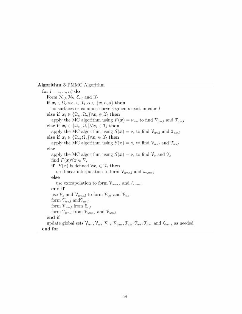
Algorithm 3 PMMC Algorithm

for l = 1, ..., n3c do

Form Nc,l,Nli,Ec,l and Xl

if xi ∈ Ωα∀xi ∈ Xl, α ∈ w, n, s thenno surfaces or common curve segments exist in cube l

else if xi ∈ Ωw,Ωn∀xi ∈ Xl thenapply the MC algorithm using F (x) = νwn to find Vwn,l and Twn,l

else if xi ∈ Ωw,Ωs∀xi ∈ Xl thenapply the MC algorithm using S(x) = νs to find Vws,l and Tws,l

else if xi ∈ Ωn,Ωs∀xi ∈ Xl thenapply the MC algorithm using S(x) = νs to find Vns,l and Tns,l

elseapply the MC algorithm using S(x) = νs to find Vs and Tsfind F (x)∀x ∈ Vs

if F (x) is defined ∀xi ∈ Xl thenuse linear interpolation to form Vwns,l and Lwns,l

elseuse extrapolation to form Vwns,l and Lwns,l

end ifuse Vs and Vwns,l to form Vws and Vns

form Tws,l andTns,lform Vwn,l from Ec,lform Twn,l from Vwns,l and Vwn,l

end ifupdate global sets Vwn,Vws,Vns,Vwns,Twn,Tws,Tns, and Lwns as needed

end for

58

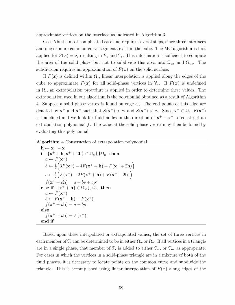
approximate vertices on the interface as indicated in Algorithm 3.

Case 5 is the most complicated case and requires several steps, since three interfaces

and one or more common curve segments exist in the cube. The MC algorithm is first

applied for S(x) = νs resulting in Vs and Ts. This information is sufficient to compute

the area of the solid phase but not to subdivide this area into Ωws and Ωns. The

subdivision requires an approximation of F (x) on the solid surface.

If F (x) is defined within Ωs, linear interpolation is applied along the edges of the

cube to approximate F (x) for all solid-phase vertices in Vs. If F (x) is undefined

in Ωs, an extrapolation procedure is applied in order to determine these values. The

extrapolation used in our algorithm is the polynomial obtained as a result of Algorithm

4. Suppose a solid phase vertex is found on edge eli. The end points of this edge are

denoted by x+ and x− such that S(x+) > νs and S(x−) < νs. Since x− ∈ Ωs, F (x−)

is undefined and we look for fluid nodes in the direction of x+ − x− to construct an

extrapolation polynomial f . The value at the solid phase vertex may then be found by

evaluating this polynomial.

Algorithm 4 Construction of extrapolation polynomial

h← x+ − x−

if x+ + h,x+ + 2h ∈ Ωw

⋃Ωn then

a← F (x+)

b← 12

(3F (x+)− 4F (x+ + h) + F (x+ + 2h)

)c← 1

2

(F (x+)− 2F (x+ + h) + F (x+ + 2h)

)f(x+ + ρh) = a+ bρ+ cρ2

else if x+ + h ∈ Ωw

⋃Ωn then

a← F (x+)b← F (x+ + h)− F (x+)f(x+ + ρh) = a+ bρ

elsef(x+ + ρh) = F (x+)

end if

Based upon these interpolated or extrapolated values, the set of three vertices in

each member of Ts can be determined to be in either Ωw or Ωn. If all vertices in a triangle

are in a single phase, that member of Ts is added to either Tws or Tns as appropriate.

For cases in which the vertices in a solid-phase triangle are in a mixture of both of the

fluid phases, it is necessary to locate points on the common curve and subdivide the

triangle. This is accomplished using linear interpolation of F (x) along edges of the

59

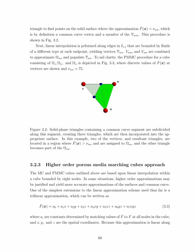
triangle to find points on the solid surface where the approximation F (x) = νwn, which

is by definition a common curve vertex and a member of the Vwns. This procedure is

shown in Fig. 3.2.

Next, linear interpolation is peformed along edges in Ec,l that are bounded by fluids

of a different type at each endpoint, yielding vertices Vwn. Vwns and Vwn are combined

to approximate Ωwn and populate Twn. To aid clarity, the PMMC procedure for a cube

consisting of Ωs,Ωw, and Ωn is depicted in Fig. 3.3, where discrete values of F (x) at

vertices are shown and νwn = 75.

Figure 3.2: Solid-phase triangles containing a common curve segment are subdividedalong this segment, creating three triangles, which are then incorporated into the ap-propriate surface. In this example, two of the vertices, and resultant triangles, arelocated in a region where F (x) > νwn and are assigned to Ωns, and the other trianglebecomes part of the Ωws.

3.2.3 Higher order porous media marching cubes approach

The MC and PMMC cubes outlined above are based upon linear interpolation within

a cube bounded by eight nodes. In some situations, higher order approximations may

be justified and yield more accurate approximations of the surfaces and common curve.

One of the simplest extensions to the linear approximation scheme used thus far is a

trilinear approximation, which can be written as

F (x) = a0 + a1x+ a2y + a3z + a4xy + a5xz + a6yz + a7xyz (3.3)

where ai are constants determined by matching values of F to F at all nodes in the cube,

and x, y, and z are the spatial coordinates. Because this approximation is linear along

60

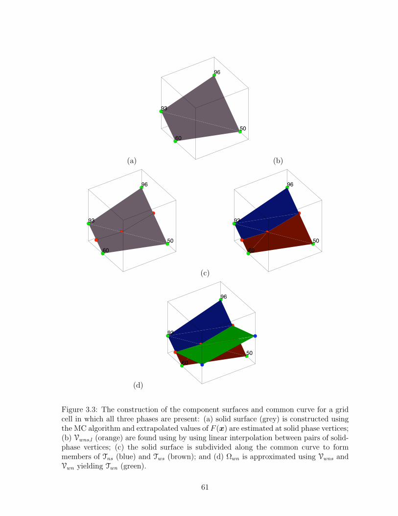
(a) (b)

(c)

(d)

Figure 3.3: The construction of the component surfaces and common curve for a gridcell in which all three phases are present: (a) solid surface (grey) is constructed usingthe MC algorithm and extrapolated values of F (x) are estimated at solid phase vertices;(b) Vwns,l (orange) are found using by using linear interpolation between pairs of solid-phase vertices; (c) the solid surface is subdivided along the common curve to formmembers of Tns (blue) and Tws (brown); and (d) Ωwn is approximated using Vwns andVwn yielding Twn (green).

61

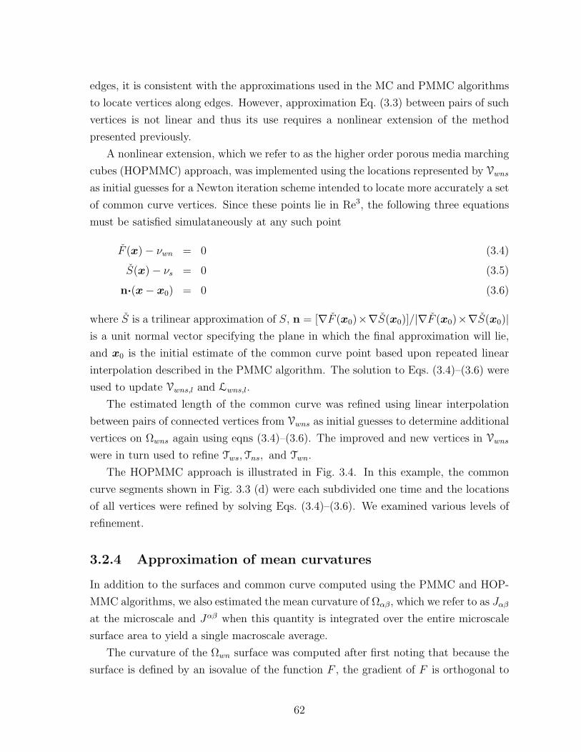
edges, it is consistent with the approximations used in the MC and PMMC algorithms

to locate vertices along edges. However, approximation Eq. (3.3) between pairs of such

vertices is not linear and thus its use requires a nonlinear extension of the method

presented previously.

A nonlinear extension, which we refer to as the higher order porous media marching

cubes (HOPMMC) approach, was implemented using the locations represented by Vwns

as initial guesses for a Newton iteration scheme intended to locate more accurately a set

of common curve vertices. Since these points lie in Re3, the following three equations

must be satisfied simulataneously at any such point

F (x)− νwn = 0 (3.4)

S(x)− νs = 0 (3.5)

n·(x− x0) = 0 (3.6)

where S is a trilinear approximation of S, n = [∇F (x0)×∇S(x0)]/|∇F (x0)×∇S(x0)|is a unit normal vector specifying the plane in which the final approximation will lie,

and x0 is the initial estimate of the common curve point based upon repeated linear

interpolation described in the PMMC algorithm. The solution to Eqs. (3.4)–(3.6) were

used to update Vwns,l and Lwns,l.

The estimated length of the common curve was refined using linear interpolation

between pairs of connected vertices from Vwns as initial guesses to determine additional

vertices on Ωwns again using eqns (3.4)–(3.6). The improved and new vertices in Vwns

were in turn used to refine Tws,Tns, and Twn.

The HOPMMC approach is illustrated in Fig. 3.4. In this example, the common

curve segments shown in Fig. 3.3 (d) were each subdivided one time and the locations

of all vertices were refined by solving Eqs. (3.4)–(3.6). We examined various levels of

refinement.

3.2.4 Approximation of mean curvatures

In addition to the surfaces and common curve computed using the PMMC and HOP-

MMC algorithms, we also estimated the mean curvature of Ωαβ, which we refer to as Jαβ

at the microscale and Jαβ when this quantity is integrated over the entire microscale

surface area to yield a single macroscale average.

The curvature of the Ωwn surface was computed after first noting that because the

surface is defined by an isovalue of the function F , the gradient of F is orthogonal to

62

Figure 3.4: Refinement of the common curve resulting from a single subdivision of thecommon curve line segments shown in Fig. 3.3 (d) and refinement of all locations usingthe HOPMMC approach.

Ωwn. Thus the unit normal was computed as:

nwn =∇F|∇F |

(3.7)

From Eq. (3.7), the mean curvature Jwn = ∇·nwn at points on Ωwn may be calcu-

lated as

Jwn = ∇· ∇F|∇F |

=(Fxx(F

2y + F 2

z ) + Fyy(F2x + F 2

z ) + Fzz(F2x + F 2

y )− 2FxyFxFy

−2FyzFyFz − 2FxzFxFz

)/(F 2

x + F 2y + F 2

z )3/2 (3.8)

where the subscripts denote differentiation of F .

Eq. (3.8) was approximated using centered difference approximations to compute

all needed derivatives of F at all nodes in a cube. The values of these derivatives were

then used to linearly interpolate values at the vertices Vwn,l and used to evaluate Jwn at

these vertices. Jwn was computed as an area-weighted average over the entire domain

Jwn =

∫Ωwn

JwndS∫Ωwn

dS. (3.9)

Using the surfaces constructed with the PMMC approach, these integrals can be eval-

uated numerically. Curvatures Jws and Jns were computed using a similar approach.

63

3.2.5 Data source

In many cases, raw data will not be in the format required by the PMMC algorithm. In

this section, we discuss schemes that allow us to obtain input data in the proper format

from various sources. Generally, two primary challenges must be addressed in order to

apply this approach correctly: (1) functions F and S must be identified and measured

to determine their values at nodes inMh, and (2) appropriate isovalues that correspond

to the surfaces of interest must be identified. In practice, the functions F and S will

correspond to different physical quantities depending on the origin of the data. It is

not feasible to develop well-defined guidelines regarding the data formatting issues for

all possible situations. Instead, we provide a selection of example cases corresponding

to likely scenarios that give insight into considerations that also apply to more general

circumstances.

(a) (b)

Figure 3.5: Slice of a porous medium data set generated using the LB method: (a) Fis comprised of the fluid density distribution and shown by color shading, and (b) theknown location of a spherical solid-phase is used to create a signed-distance functionand Ωs is represented in black after being constructed using the PMMC algorithm.

Fig. 3.5 (a) shows a slice of a porous medium data set in which F (x) is the fluid

density determined from a LB simulation. A value of zero is assigned to all nodes that

are in Ωs to denote that the fluid density is undefined in this region. In this case, the

position of the solid phase is known a priori, and the solid surface may be reconstructed

by using this knowledge to determine S(x). The solid phase is composed of nS spheres

with centers cs and radii rs, where s = 1, . . . , nS, and we choose S(x) to be the signed

distance from a point x in Mh to the nearest surface of the solid, which we compute

64

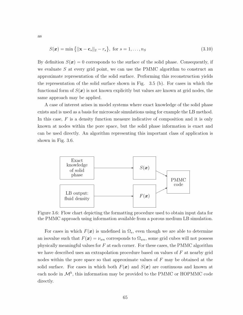
as

S(x) = min||x− cs||2 − rs

, for s = 1, . . . , nS (3.10)

By definition S(x) = 0 corresponds to the surface of the solid phase. Consequently, if

we evaluate S at every grid point, we can use the PMMC algorithm to construct an

approximate representation of the solid surface. Performing this reconstruction yields

the representation of the solid surface shown in Fig. 3.5 (b). For cases in which the

functional form of S(x) is not known explicitly but values are known at grid nodes, the

same approach may be applied.

A case of interest arises in model systems where exact knowledge of the solid phase

exists and is used as a basis for microscale simulations using for example the LB method.

In this case, F is a density function measure indicative of composition and it is only

known at nodes within the pore space, but the solid phase information is exact and

can be used directly. An algorithm representing this important class of application is

shown in Fig. 3.6.

Exactknowledge

of solidphase

LB output:fluid density

-

-

S(x)

F (x)

HHHj

*

PMMCcode

Figure 3.6: Flow chart depicting the formatting procedure used to obtain input data forthe PMMC approach using information available from a porous medium LB simulation.

For cases in which F (x) is undefined in Ωs, even though we are able to determine

an isovalue such that F (x) = νwn corresponds to Ωwn, some grid cubes will not possess

physically meaningful values for F at each corner. For these cases, the PMMC algorithm

we have described uses an extrapolation procedure based on values of F at nearby grid

nodes within the pore space so that approximate values of F may be obtained at the

solid surface. For cases in which both F (x) and S(x) are continuous and known at

each node inMh, this information may be provided to the PMMC or HOPMMC code

directly.

65

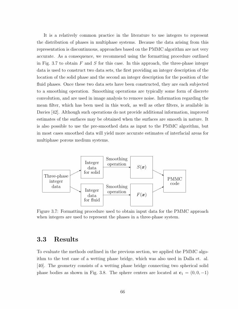
It is a relatively common practice in the literature to use integers to represent

the distribution of phases in multiphase systems. Because the data arising from this

representation is discontinuous, approaches based on the PMMC algorithm are not very

accurate. As a consequence, we recommend using the formatting procedure outlined

in Fig. 3.7 to obtain F and S for this case. In this approach, the three-phase integer

data is used to construct two data sets, the first providing an integer description of the

location of the solid phase and the second an integer description for the position of the

fluid phases. Once these two data sets have been constructed, they are each subjected

to a smoothing operation. Smoothing operations are typically some form of discrete

convolution, and are used in image analysis to remove noise. Information regarding the

mean filter, which has been used in this work, as well as other filters, is available in

Davies [42]. Although such operations do not provide additional information, improved

estimates of the surfaces may be obtained when the surfaces are smooth in nature. It

is also possible to use the pre-smoothed data as input to the PMMC algorithm, but

in most cases smoothed data will yield more accurate estimates of interfacial areas for

multiphase porous medium systems.

Three-phaseintegerdata

*

HHHj

Integerdata

for solid

Integerdata

for fluid

-

-

Smoothingoperation

Smoothingoperation

S(x)

F (x)

HHHj

*

PMMCcode

Figure 3.7: Formatting procedure used to obtain input data for the PMMC approachwhen integers are used to represent the phases in a three-phase system.

3.3 Results

To evaluate the methods outlined in the previous section, we applied the PMMC algo-

ithm to the test case of a wetting phase bridge, which was also used in Dalla et. al.

[40]. The geometry consists of a wetting phase bridge connecting two spherical solid

phase bodies as shown in Fig. 3.8. The sphere centers are located at c1 = (0, 0,−1)

66

and c2 = (0, 0, 1) and have radii r1 = r2 = Rs. The signed distance function given by

Eq. (3.10) was used to obtain S(x). F (x) is given by:

F (x) =

νwn +√x2 + y2 +

√R2 − z2 − (R + rc) if |z| ≤ L/2

νwn − a+(x2 + y2 +

(|z| − L/2

)2)1/2

if |z| > L/2(3.11)

where R is the radius of curvature in any plane intersecting with the z axis and rc is the

minimum throat radius. The specification of these two parameters with Rs completely

defines the bridge geometry. It follows that the length of the bridge L and radial

distance of the contact curve from the z-axis a can be expressed in terms of Rs, R, and

rc using basic trigonometry.

Figure 3.8: Slice of the bridge geometry shown with values of F computed using νwn =0.5, Rs = 0.5, rc = 0.2, and R = 1.4.

From this geometry, values for εwn, εns, εws, and εwns can be calculated analytically

as

εns =4πRs

V

(Rs −

L

2+ 1)

(3.12)

εws =4πRs

V

(Rs +

L

2− 1)

(3.13)

67

εwns =4πa

V(3.14)

where V is the volume of the region analyzed. Note that Eqs. (3.12) and (3.13) involve

expressions for the area of a sphere and spherical cap, and Eq. (3.14) is the length of

the perimeter of two circles of radius a. The surface area of the bridge is computed by

evaluating the surface integral:

εwn =1

V

(∫∫S

|τu × τv|u. v.

)

=4πR

V

[(R + rc) arcsin

( L2R

)− L

2

](3.15)

where τu and τv are tangent vectors for the surface parameterized by u and v.

The approach of [40] uses the MC algorithm to approximate the total wetting, non-

wetting, and solid surfaces from integer valued data sets. The interfacial area εwn is

then computed by using the surface areas of these objects. Fig. 3.9 shows the relative

errors for this approach in comparison with errors for the PMMC method on the same

geometry.

It is a relatively common practice in the literature to represent a multiphase system

by using integers to mark the positions of the phases. For this reason, we tested the

PMMC approach described in §3.2.2 using input data in this form, as well as data from

the continuous functions described in Eqs. (3.10) and (3.11). For the integer data, we

used

S(x) =

−1 if S(x) < 0

1 otherwise(3.16)

F (x) =

1 if F (x) < νwn

2 otherwise(3.17)

Data generated in this manner was used as input to the PMMC algorithm along with

the isovalue for Ωws. We also subjected S(x) and F (x) to smoothing algorithms as

described in §3.2.5. In both cases, the isovalues for the fluid phases were determined

to be midway between the integer values. Relative errors for this test case are plotted

in Fig. 3.10 (a), (b) and (c). The ratio of the minimum radius of curvature to the grid

spacing for each object of interest is plotted on the abscissa. Filtering the integer data

as depicted in Fig. 3.7 lead to smooth surfaces and estimates of their measure converged

68

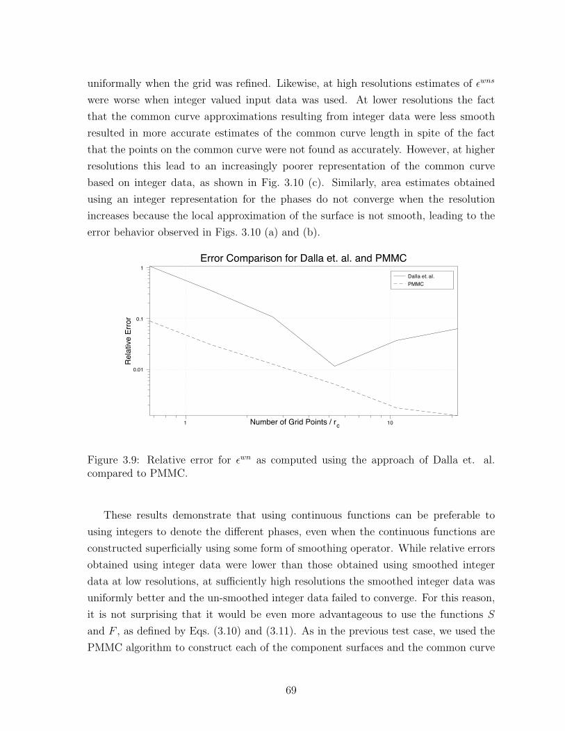
uniformally when the grid was refined. Likewise, at high resolutions estimates of εwns

were worse when integer valued input data was used. At lower resolutions the fact

that the common curve approximations resulting from integer data were less smooth

resulted in more accurate estimates of the common curve length in spite of the fact

that the points on the common curve were not found as accurately. However, at higher

resolutions this lead to an increasingly poorer representation of the common curve

based on integer data, as shown in Fig. 3.10 (c). Similarly, area estimates obtained

using an integer representation for the phases do not converge when the resolution

increases because the local approximation of the surface is not smooth, leading to the

error behavior observed in Figs. 3.10 (a) and (b).

Figure 3.9: Relative error for εwn as computed using the approach of Dalla et. al.compared to PMMC.

These results demonstrate that using continuous functions can be preferable to

using integers to denote the different phases, even when the continuous functions are

constructed superficially using some form of smoothing operator. While relative errors

obtained using integer data were lower than those obtained using smoothed integer

data at low resolutions, at sufficiently high resolutions the smoothed integer data was

uniformly better and the un-smoothed integer data failed to converge. For this reason,

it is not surprising that it would be even more advantageous to use the functions S

and F , as defined by Eqs. (3.10) and (3.11). As in the previous test case, we used the

PMMC algorithm to construct each of the component surfaces and the common curve

69

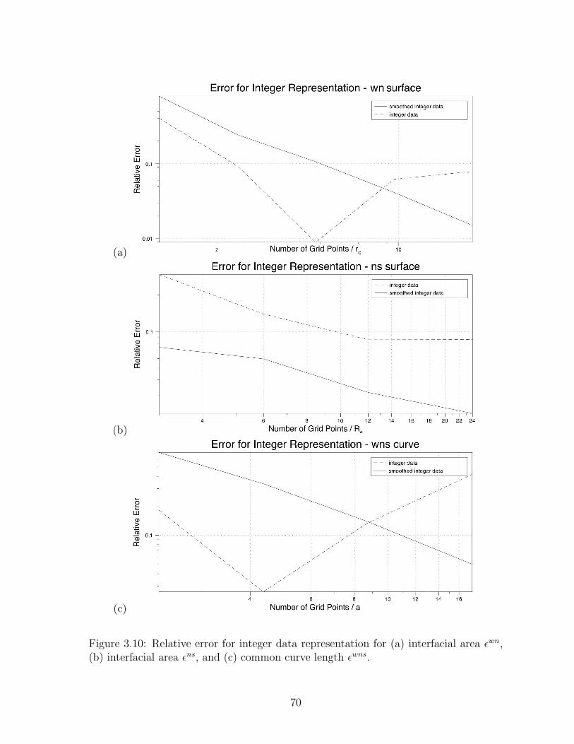
(a)

(b)

(c)

Figure 3.10: Relative error for integer data representation for (a) interfacial area εwn,(b) interfacial area εns, and (c) common curve length εwns.

70

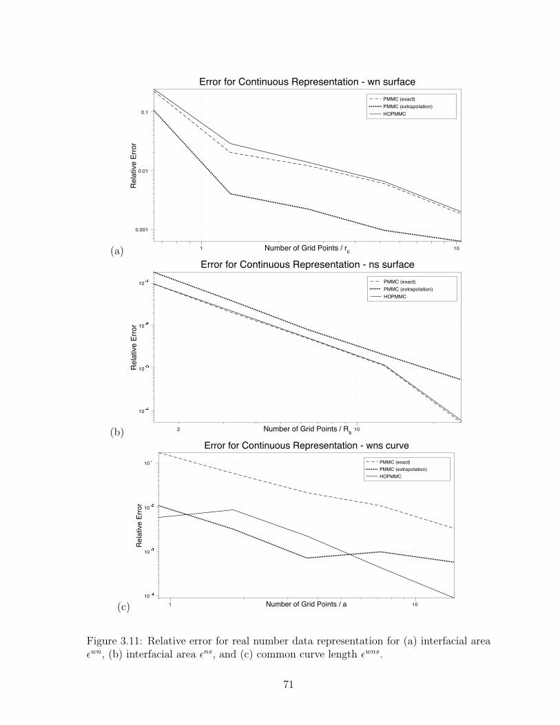
(a)

(b)

4 3 2 1

(c)

4 3 2 1

Figure 3.11: Relative error for real number data representation for (a) interfacial areaεwn, (b) interfacial area εns, and (c) common curve length εwns.

71

using S and F in conjunction with the formatting procedure outlined in Fig. 3.6. Errors

for εwn, εns, and εwns are plotted in Fig. 3.11 (a), (b) and (c). For the results labeled

exact, we used a direct evaluation of F at all mesh points. For the results labeled

extrapolation, we extrapolated values of F for all locations within the solid phase

using the approach detailed in Algorithm 4. Additionally, we applied the HOPMMC

approach discussed in §3.2.3 using Newton’s method to obtain an updated position for

each point on the common curve. In addition to the points found using the PMMC

approach, each common curve segment was subdivided to provide one additional point

per line segment. In these plots, F and S were trilinear polynomials chosen to match

the values of F and S exactly at each of the cube corners.

3.4 Discussion

Our analysis of the test case presented in the previous section provides a number of

insights as to what may be expected from the PMMC approach. First and foremost,

it is clear that this method is capable of providing accurate representations of the

component surfaces and common curve for multiphase systems, something that is not

possible using the standard MC algorithm alone. Second, it is also clear that the use

of continuous functions is superior to the use of integers to represent the positions of

the phases, despite the fact that integer representations are used with some regularity

[40, 105]. The continuous functions used may be obtained from sources such as fluid

density, photon absorption data for experimental systems, distance functions, and even

integer data subjected to smoothing operations.

In many cases, particularly pertaining to experimental data, the application of

smoothing operations is necessary to remove noise and cannot be avoided. A drawback

to applying such procedures when not needed is that they remove information from the

system, thereby making it more difficult to resolve features that are small relative to

the grid spacing. For this reason, it is wise to apply smoothing operations only when

necessary.

The results of the previous section provide a general idea of the level of resolution

needed to resolve features of a particular size. It is important to consider the relative

size of various features when viewing the error plots in order ascertain what error

should be anticipated when analyzing a porous medium data file. There are several

different length scales of interest that could be useful in determining how these results

should be interpreted. Features that are smaller than individual grid cubes cannot be

72

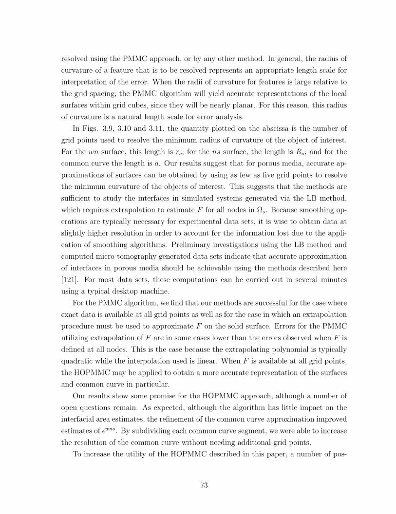
resolved using the PMMC approach, or by any other method. In general, the radius of

curvature of a feature that is to be resolved represents an appropriate length scale for

interpretation of the error. When the radii of curvature for features is large relative to

the grid spacing, the PMMC algorithm will yield accurate representations of the local

surfaces within grid cubes, since they will be nearly planar. For this reason, this radius

of curvature is a natural length scale for error analysis.

In Figs. 3.9, 3.10 and 3.11, the quantity plotted on the abscissa is the number of

grid points used to resolve the minimum radius of curvature of the object of interest.

For the wn surface, this length is rc; for the ns surface, the length is Rs; and for the

common curve the length is a. Our results suggest that for porous media, accurate ap-

proximations of surfaces can be obtained by using as few as five grid points to resolve

the minimum curvature of the objects of interest. This suggests that the methods are

sufficient to study the interfaces in simulated systems generated via the LB method,

which requires extrapolation to estimate F for all nodes in Ωs. Because smoothing op-

erations are typically necessary for experimental data sets, it is wise to obtain data at

slightly higher resolution in order to account for the information lost due to the appli-

cation of smoothing algorithms. Preliminary investigations using the LB method and

computed micro-tomography generated data sets indicate that accurate approximation

of interfaces in porous media should be achievable using the methods described here

[121]. For most data sets, these computations can be carried out in several minutes

using a typical desktop machine.

For the PMMC algorithm, we find that our methods are successful for the case where

exact data is available at all grid points as well as for the case in which an extrapolation

procedure must be used to approximate F on the solid surface. Errors for the PMMC

utilizing extrapolation of F are in some cases lower than the errors observed when F is

defined at all nodes. This is the case because the extrapolating polynomial is typically

quadratic while the interpolation used is linear. When F is available at all grid points,

the HOPMMC may be applied to obtain a more accurate representation of the surfaces

and common curve in particular.

Our results show some promise for the HOPMMC approach, although a number of

open questions remain. As expected, although the algorithm has little impact on the

interfacial area estimates, the refinement of the common curve approximation improved

estimates of εwns. By subdividing each common curve segment, we were able to increase

the resolution of the common curve without needing additional grid points.

To increase the utility of the HOPMMC described in this paper, a number of pos-

73

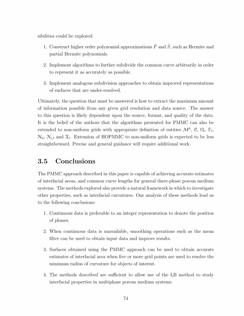
sibilities could be explored:

1. Construct higher order polynomial approximations F and S, such as Hermite and

partial Hermite polynomials.

2. Implement algorithms to further subdivide the common curve arbitrarily in order

to represent it as accurately as possible.

3. Implement analogous subdivision approaches to obtain improved representations

of surfaces that are under-resolved.

Ultimately, the question that must be answered is how to extract the maximum amount

of information possible from any given grid resolution and data source. The answer

to this question is likely dependent upon the source, format, and quality of the data.

It is the belief of the authors that the algorithms presented for PMMC can also be

extended to non-uniform grids with appropriate definition of entities Mh, C, Ωl, Γl,

Nli, Nc,l and Xl. Extension of HOPMMC to non-uniform grids is expected to be less

straightforward. Precise and general guidance will require additional work.

3.5 Conclusions

The PMMC approach described in this paper is capable of achieving accurate estimates

of interfacial areas, and common curve lengths for general three-phase porous medium

systems. The methods explored also provide a natural framework in which to investigate

other properties, such as interfacial curvatures. Our analysis of these methods lead us

to the following conclusions:

1. Continuous data is preferable to an integer representation to denote the position

of phases.

2. When continuous data is unavailable, smoothing operations such as the mean

filter can be used to obtain input data and improve results.

3. Surfaces obtained using the PMMC approach can be used to obtain accurate

estimates of interfacial area when five or more grid points are used to resolve the

minimum radius of curvature for objects of interest.

4. The methods described are sufficient to allow use of the LB method to study

interfacial properties in multiphase porous medium systems.

74

The proposed algorithms represent a substantial improvement over the standard MC

algorithm, which was studied in [40]. In addition to interfaces, the PMMC approach

also allows extraction of common curves so that they can be studied in the context of

evolving theories.

3.6 Additional Morphological Properties

3.6.1 Contact Angle

The contact angle θwns is an important geometric quantity in multiphase porous media

as it provides a boundary condition for the interfacial profile. In a multiphase system,

the contact angle is related to the various surface energies γwn, γws, andγns as given by

Young’s equation:

γwn cos θwns = γns − γws. (3.18)

The contact angle may be computed geometrically by relating its value to the normal

vectors to the fluid and solid surfaces, denoted by nwn and ns:

cos θwns = nwn · ns. (3.19)

The results of §3.2.4 demonstrate how the geometric surface quantities can be evaluated

based on the functions F and S. The solid normal vector be computed based on the

analog of Eq. (3.7):

ns =∇S|∇S|

. (3.20)

With the normal vectors defined in terms of F and S, the contact angle can be nu-

merically evaluated by using a second order finite difference stencil to evaluate the

derivatives and applying linear interpolation to obtain the contact angle values along

the common curve Ωwns. The maximum relative error is shown in Fig. (3.13) for a

sequence of systems in which F and S are assigned from distance functions. In general,

contact angle approximations will be less accurate when F and S can not be prescribed

from a distance function.

75

ns

nwn

θwns

Wetting Phase

Non-wetting Phase

Solid Phase

Figure 3.12: Contact angle in a three-phase system.

θwns

= π/8

θwns

= π/4

θwns

= π/3

10

10-4

10-3

10-2

10-1

Error for Contact Angle Measurement

Resolution

Maxim

um

Rela

tive E

rror

Figure 3.13: Maximum relative error for estimated contact angle

76

3.7 Collective Rearrangement Sphere Packing Al-

gorithm

(a) (b)0 0.02 0.04 0.06 0.08 0.1 0.12 0.14 0.16 0.18 0.2 0.22

0

2

4

6

8

10

12

14

16

18

20

Distribution of Radii for Simulated System

r

Figure 3.14: (a) Sphere packing of 250 lognormally distributed sphere with φ = 0.34722(b) Histogram of radii plotted beside the lognormal distribution with µ = −2.76, σ2 =0.2.

Pore-scale simulations of flow in porous media require precise information about

solid boundaries in order to provide boundary conditions to the flow solver. Sphere

packings provide a realistic surrogate porous media which are often utilized for pore-

scale flow simulation [].

The sphere packing code utilizes the algorithm used by Williams and Philipse to

generate packings of sphereocylinders [194]. The algorithm has been modified to sup-

port generation of packings for systems of spheres with lognormally distributed radii,

and to provide control over the final porosity of the packing. The major steps are

summarized as follows:

1. Instantiate a system of spheres, i = 1, 2, . . . , Ns :

• c(i)x U [0, `x]

• c(i)y U [0, `y]

• c(i)z U [0, `z]

• log(r(i))n([)µ, σ2]

2. Eliminate overlaps between spheres (see Williams and Philipse)

77

3. Increase size of radii:

• r(i) ← α(f)r(i)

• µ← µ+ log(α(f))

It is easy to verify that rescaling of the radii by a constant factor α(f) preserves

the lognormal distribution variance σ2 and that the mean µ will increase by log(α)

each time the radii are rescaled. This means that while σ2 is specified as an input

parameter, µ is not known until the simulation completes. Note that it is not possible

to independently specify µ, σ2 and φ. Given σ2, the final value of µ can be estimated

based on the target porosity φtarget. The expected volume of the lognormal packing is:

4πNs

3E[r3] = 4πNs

3exp

(3µ+ 9

2σ2)

(3.21)

To accelerate convergence, the spheres are divided into a collection of cells which

consist of equally-sized sub-domains. This is a standard optimization for N -particle

methods. The number of cells in each direction is determined from line 6 of the input

file. Each cell contains a list of the spheres with centroids contained within the physical

boundaries of the cell. For a given sphere, potential overlaps are considered only from

the neighboring cells. The code is accelerated significantly by increasing the number

of cells, thereby decreasing the length of the search path required when computing

overlaps. However, this optimization can lead to oversights in the overlap computation

if the maximum radius exceeds one half of the cell width, as shown in Fig. (??) (a).

The maximum radius is checked after the simulation completes, and a warning message

is issued if the maximum radius is too large based on the cell width:

The well-known limit for a close packing of equal sized spheres is φ ≈ 0.36. Likewise,

the maximum stable porosity for a homogeneous sphere packing is φ ≈ 0.44–0.47,

with a coordination number of approximately six [48]. Each of these results has been

reproduced with this packing code.

78

Chapter 4

Direction-Dependent Flow in

Porous Media

4.1 Introduction

Modeling of single-phase flow in porous media is accomplished by an almost universal

approach that makes use of Darcy’s law at low flow rates [41] as well as nonlinear ex-

tensions that apply at higher flow rates [52]. Recent work has focused on formulating a

rigorous theoretical basis for these empirically determined expressions and establishing

a firm connection between spatial scales [18, 34, 67, 71, 111, 60]. Development of this

theoretical foundation has been complemented by application of highly-resolved numer-

ical solutions to the Navier-Stokes equations that have been used to study macroscopic

flow behavior from the pore-scale [4, 51, 78, 107, 112]. These efforts have contributed

important insights into the microscopic origins of macroscopic phenomena, leading to a

more nuanced understanding of single-phase flow. This work supports classification of

single-phase flows into three primary regimes: a Darcy regime that can be linked with

microscopic Stokes flow, a transition regime corresponding with moderate Reynolds

numbers and the onset of inertial effects, and an inertial regime in which inertial effects

contribute strongly to the macroscopic flow behavior.

For Stokes flow, the microscopic velocity structure is independent of the Reynolds

number Re. This means that if the velocity structure is known for a single value of Re,

it may be obtained for any Re by a linear rescaling of the velocity field. Since the flow

field is itself linear, it follows that the macroscopic flow will also be linear, in accordance

with Darcy’s law. However as Re increases, the microscopic Stokes’ flow solution does

not apply. Numerical solutions to the Navier-Stokes equations demonstrate that this

breakdown corresponds to the formation of eddies within the microscopic flow field,

ultimately resulting in nonlinear behavior at the macroscale [53, 142]. These micro-

scopic origins of macroscopic nonlinearity have interesting implications for anisotropic

flows. At the pore-scale, details of the pore morphology and topology determine the

formation, location and size of eddies within a particular porous medium flow. If the

grain shapes are not symmetric with respect to the flow direction, the structure and po-

sition of eddies may exhibit directional dependence. In such situations, it is reasonable

to expect a flow reversal to have a corresponding effect on macroscopic nonlinearity.

Existing forms of non-Darcy flow models fail to anticipate this possibility, creating a

scenario in which the coefficients for a particular porous medium will depend on the

flow direction.

At the pore-scale, flow processes are strongly dependent on details of the mor-

phology and topology of the pore structure. However, the complexity of real porous

media dictates that many details of pore structure are often inaccessible. As a conse-

quence, construction of representative macroscopic forms relies in part upon an ability

to approximate the complexity of real porous medium pore structure based upon only a

few morphological and topological measures. Unfortunately, identification of such mea-

sures is not always obvious. Thermodynamically constrained averaging theory (TCAT),

which has been used to derive Darcy’s Law [60], represents a theoretical framework for

deriving macroscopic flow models by systematically upscaling a microscale, or pore

scale, model [59, 127]. Various geometrical measures arise as a consequence of the av-

eraging, but they do not always appear in the final flow equations. Nevertheless, these

ancillary parameters represent potentially important quantitative measures of the mor-

phology and topology of the pore structure. Incorporation of these quantities provides

a systematic way to improve the macroscopic description of processes influenced by

aspects of the pore morphology and topology that are often ignored.

The overall goal of this manuscript is to examine the microscopic and macroscopic

consequences of reversing the flow direction in simple asymmetric porous media. Appli-

cation of numerical simulations at the pore-scale will serve to demonstrate that reversal

of the flow direction can lead to significant differences in the velocity structure at the

pore-scale, an effect which has a direct impact on the macroscopic behavior. In order

to account for this phenomenon, we suggest ways to incorporate this behavior into

macroscopic models. The primary objectives are:

1. to propose an alternative form for the momentum equation (extended Darcy’s

law) that accounts for extended anisotropy due to grain asymmetry;

80

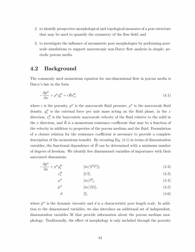
2. to identify prospective morphological and topological measures of a pore structure

that may be used to quantify the symmetry of the flow field; and

3. to investigate the influence of asymmetric pore morphologies by performing pore-

scale simulations to support macroscopic non-Darcy flow analysis in simple, pe-

riodic porous media.

4.2 Background

The commonly used momentum equation for one-dimensional flow in porous media is

Darcy’s law in the form

−∂pw

∂x+ ρwgwx = εRvwx , (4.1)

where ε is the porosity, pw is the macroscale fluid pressure, ρw is the macroscale fluid

density, gwx is the external force per unit mass acting on the fluid phase, in the x

direction, vwx is the barycentric macroscale velocity of the fluid relative to the solid in

the x direction, and R is a momentum resistance coefficient that may be a function of

the velocity in addition to properties of the porous medium and the fluid. Formulation

of a closure relation for the resistance coefficient is necessary to provide a complete

description of the momentum transfer. By recasting Eq. (4.1) in terms of dimensionless

variables, the functional dependence of R can be determined with a minimum number

of degrees of freedom. We identify five dimensioned variables of importance with their

associated dimensions:

−∂pw

∂x+ ρwgwx [m/(l2t2)], (4.2)

vwx [l/t], (4.3)

ρw [m/l3], (4.4)

µw [m/(lt)], (4.5)

d [l], (4.6)

where µw is the dynamic viscosity and d is a characteristic pore length scale. In addi-

tion to the dimensioned variables, we also introduce an additional set of independent,

dimensionless variables M that provide information about the porous medium mor-

phology. Traditionally, the effect of morphology is only included through the porosity

81

ε. We consider the flow to depend on M, a set of variables that includes ε as well as

other variables to be determined. Specification of these additional variables provides a

general mechanism to incorporate aspects of the morphology and topology of the pore

space that influence macroscopic flow behavior but are neglected in traditional model

forms.

Since there are three dimensions involved and five dimensioned variables, we can

form two independent, dimensionless groups in addition to the set of inherently non-

dimensional quantities in M. Select these as:

Π1 =

(−∂p

w

∂x+ ρwgwx

)db1(µw)c1(vwx )e1 , (4.7)

Π2 = ρwdb2 (µw)c2(vwx)e2 . (4.8)

Solution for the values of the exponents that assure non-dimensionality of the group of

parameters gives:

Π1 =

(−∂p

w

∂x+ ρwgwx

)d2

vwx µw

, (4.9)

and:

Π2 =ρwvwx d

µw. (4.10)

The grouping of Π2 is the Reynolds number and will be denoted using:

Re =ρwvwx d

µw. (4.11)

It is critical to note that vwx may be either positive or negative, depending on whether

the flow is in the +x or −x direction. Consequently, the Reynolds number employed

here may take on both positive and negative values. Thus, the dimensionless equation

that arises is:

0 = Φ

(−∂p

w

∂x+ ρwgwx

)d2

vwx µw

,Re,M

. (4.12)

82

The explicit form of this equation for Π1 in terms of the other variables is:

−∂pw

∂x+ ρwgwx =

µw

d2F (Re,M) vwx , (4.13)

where F is a dimensionless function of Re and M to be determined. From the analysis

of single-fluid-phase flow that includes consideration of the entropy inequality, we know

that F ≥ 0.

By comparison with Eq. (4.1), we see that:

εRvwx =µw

d2F (Re,M) vwx , (4.14)

so that:

R =µw

εd2F (Re,M) . (4.15)

From experimental work on porous media, it is known that for small magnitudes of

Re, the resistance factor does not depend on Re. Thus we can separate the function F

into two parts: one, designated a, that depends only on the pore structure morphology

and topology measures M and one, designated B, that depends on Re as well as M

with the stipulation that when |Re| is small, the contribution of B to the value of R is

essentially zero. Thus, Eq. (4.15) becomes:

R =µw

εd2[a(M) +B (Re,M)] . (4.16)

In one sense, the purpose of this paper is to examine cases where the function B is

important for accurately describing the macroscale flow. For these cases the resistance

coefficient will also increase as the magnitude of Re increases. Since we have discussed

the fact that B(0,M) = 0, the simplest assumption for the explicit form of B would be

linear in |Re| such that:

B (Re,M) = b (M) |Re|. (4.17)

We note that this expression is linear in the absolute value of Re because the contri-

bution to resistance of higher velocity flow is positive. This expansion is a common

approach and results in the Forchheimer expression when b(M) is linearly proportional

to ε. For the case of extended anisotropy to be considered here, we add the condition

83

that besides being linear in |Re|, B is linear in Re, providing a direction-dependent

effect:

B (Re,M) = b (M) |Re|+ c (M) Re. (4.18)

Thus the resistance coefficient is:

R =µw

εd2

(a(M) + b (M) |Re|+ c (M) Re

). (4.19)

Substitution of this expression into Eq. (4.1) gives:

−∂pw

∂x+ ρwgwx =

µw

d2

(a(M) + b (M) |Re|+ c (M) Re

)vwx (4.20)

Multiplication by ρwd3/ (µw)2 allows this to be expressed as:

Fo =[a(M) + b (M) |Re|+ c (M) Re

]Re, (4.21)

where:

Fo =ρwd3

(µw)2

(−∂p

w

∂x+ ρwgwx

). (4.22)

Eq. (4.21) is similar to the Forchheimer equation in that it is quadratic in the flow

velocity. However, it will differ from the Forchheimer equation when the momentum

resistance depends on the direction of flow (i.e., the sign of Re), resulting in a non-zero

value of c. The coefficients a, b and c are medium-specific properties, as indicated by

their dependence on the set of dimensionless morphological measures M. The leading

coefficient a(M) is related to the intrinsic permeability of the medium. The parameter

b(M) determines the mean correction to Darcy’s law, which will be a positive quantity

because an increase in the flow velocity will tend to decrease the overall permeability.

The direction-dependent correction given by c(M) may be positive or negative with

|c(M)| < b(M).

84

4.3 Methods

4.3.1 Lattice Boltzmann Model

The lattice Boltzmann Method (LBM) is a well-established numerical approach for

simulation of fluid flows. For single-fluid-phase flow, the LBM may be considered as an

alternative solution procedure for the Navier-Stokes equations rooted in kinetic rather

than continuum theory. Instead of solving conservation equations to track the evolu-

tion of the fluid density and momentum, a discrete approximation of the microscopic

distribution function is used to track fluid behavior. This discrete approximation is

obtained by formulating a quadrature scheme for the microscopic velocity space, lead-

ing to a set of discrete velocities ξq and an associated set of distributions fq, where

q = 0, 1, . . . , Q − 1 [73]. The discrete distributions provide a mechanism to track the

fluid density:

ρw =

Q−1∑q=0

fq, (4.23)

and momentum:

ρwvw =

Q−1∑q=0

fqξq. (4.24)

where the subscripts on ρw and vw denote microscale quantities.

According to kinetic theory, changes to fq result from contributions of intermolecular

collisions Cq and external forces Fq. The discrete distributions can therefore be updated

by:

fq(xi + ξqδt, t+ δt) = fq(xi, t) + Cq(xi, t) + Fq. (4.25)

The form of the collision operator Cq(xi, t) is critical to proper description of the fluid

physics, and exerts a significant influence on numerical behavior [139]. Our approach

utilizes the three-dimensional, nineteen velocity vector (D3Q19) multiple-relaxation-

time (MRT) scheme described in detail by [44]. The MRT scheme considers molecular

collisions as a relaxation process in which a set of moments, constructed from the dis-

tributions, relax toward their equilibrium values. Specification of these moments along

with their equilibrium values ensures recovery of the Navier-Stokes equations. Due to

85

the locality of the left-hand side of Eq. (4.25), parallel implementations of the LBM can

achieve near-optimal scaling [137, 138]. Complex solid geometry can be accommodated

efficiently by applying the bounce-back rule to achieve a no-slip boundary condition on

the solid surface [54]. These qualities are particularly advantageous for porous medium

applications, where large domain sizes and complex solid geometry are the rule.

Description of non-Darcy flow is accomplished by simulating a sequence of steady-

state velocity fields within a specified pore structure. Each point on the non-Darcy

curve is obtained by choosing a fixed value of Fo to drive flow in the x direction.

Iterations are then carried out until the pore-scale velocity field reaches a steady-state

according to the criteria:

∑i

|vw(xi, t)− vw(xi, t− 200)||vw(xi, t)|

< 1.0× 10−7. (4.26)

Once a steady-state velocity field has been obtained, the macroscopic flow velocity vw

is obtained as the density-weighted volume average of the pore velocity u integrated

over the flow domain Ωw:

vw =

∫Ωw

ρwvw dr∫Ωw

ρw dr

= 〈vw〉Ωw,Ωw,ρw. (4.27)

Once the macroscopic velocity has been determined, Re can be computed according to

Eq. (4.11).

4.3.2 Solid Geometry

To construct flow domains in which the nonlinear behavior is likely to depend upon

the flow direction, we define porous media composed of asymmetrical, oriented solid

grains. Clearly, many asymmetrical grain shapes are possible. The objective is not to

examine a large set of such possibilities, but to investigate the hypothesized behavior by

examining some simple examples of such media. Pursuant to this goal, we consider two

simple grain shapes that lack reflection symmetry with respect to the plane orthogonal

to the flow direction. Porous media constructed using these basic grain shapes oriented

in one direction serve as the basis for this study.

The first grain shape is the smoothed triangular grain shown in Fig. (4.1). Smoothed

86

rg

wg

hg

Figure 4.1: Smoothed triangular solid grains are defined by the grain width wg, grainheight hg, and smoothing radius rg.

triangular grains are described by the grain width wg, the grain height hg, and the

smoothing radius rg. Note that reflection symmetry is present in the vertical, but not

the horizontal direction for this geometry. This grain shape is used to construct a

two-dimensional periodic packing, and its surface of revolution is used to construct a

three-dimensional packing.

It is also desirable to consider a geometry for which the asymmetry is easily quan-

tified. For this reason, we consider a case in which a single parameter controls the

symmetry of the solid grain. One such geometry is a “stretched” ellipsoid, given by:

x2

r2x

+1

1 + sx

(y2 + z2

r2d

)= 1. (4.28)

For this particular geometry, the parameter s determines how much reflection asymme-

try the grain shape will exhibit in the x direction When s = 0, the surface obtained from

Eq. (4.28) will be an ellipsoid with principle radii rx and rd. The geometry becomes

increasingly asymmetrical as s increases. This increase in asymmetry is illustrated

graphically in Fig. (4.2) (a)–(d).

4.3.3 Anti-symmetric Orientation Tensor

Thermodynamically constrained averaging theory provides a rigorous framework for

derivation of macroscopic flow equations. For single-fluid-phase flow, macroscopic quan-

tities are defined by averages over the fluid or solid phase volumes Ωf and Ωs or the

interfacial surface Ωws. Many details of the solid morphology are included implicitly

87

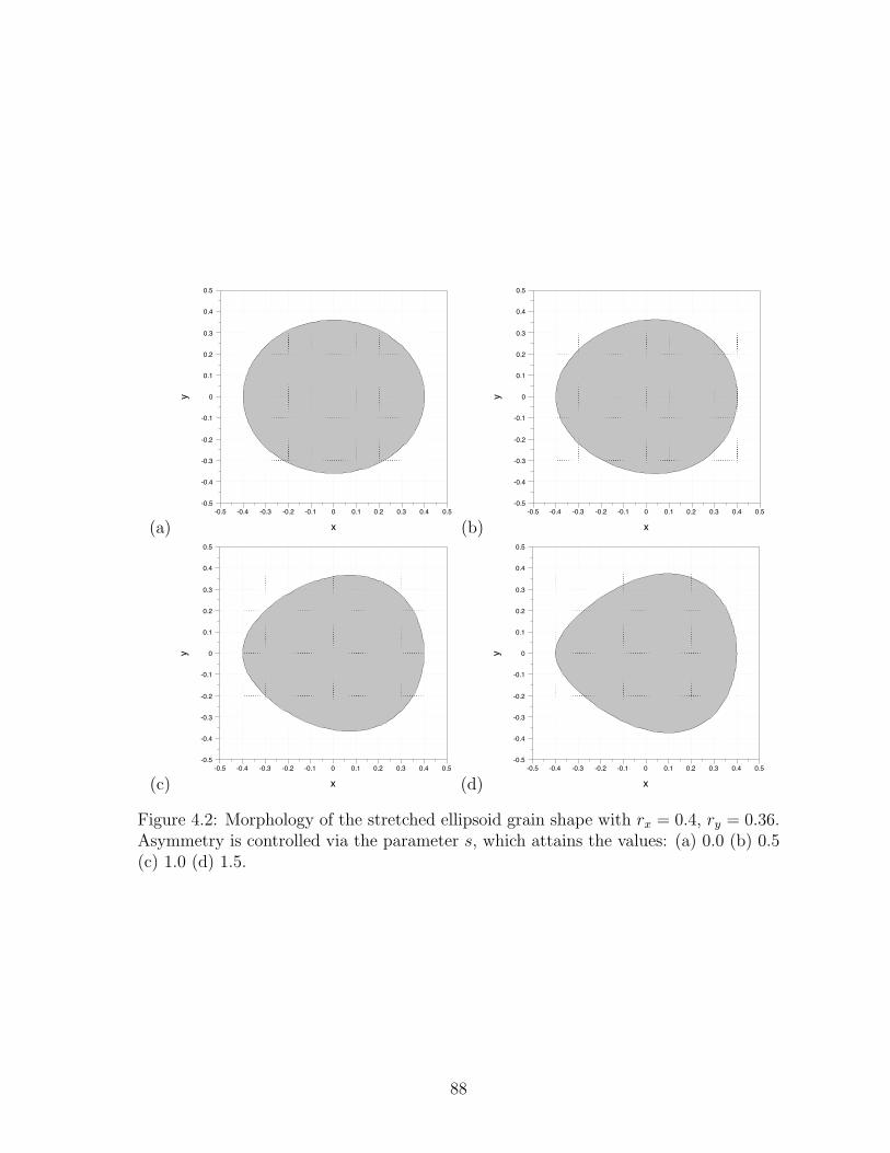
(a)-0.5 -0.4 -0.3 -0.2 -0.1 0 0.1 0.2 0.3 0.4 0.5

-0.5

-0.4

-0.3

-0.2

-0.1

0

0.1

0.2

0.3

0.4

0.5

x

y

(b)-0.5 -0.4 -0.3 -0.2 -0.1 0 0.1 0.2 0.3 0.4 0.5

-0.5

-0.4

-0.3

-0.2

-0.1

0

0.1

0.2

0.3

0.4

0.5

x

y

(c)-0.5 -0.4 -0.3 -0.2 -0.1 0 0.1 0.2 0.3 0.4 0.5

-0.5

-0.4

-0.3

-0.2

-0.1

0

0.1

0.2

0.3

0.4

0.5

x

y

(d)-0.5 -0.4 -0.3 -0.2 -0.1 0 0.1 0.2 0.3 0.4 0.5

-0.5

-0.4

-0.3

-0.2

-0.1

0

0.1

0.2

0.3

0.4

0.5

x

y

Figure 4.2: Morphology of the stretched ellipsoid grain shape with rx = 0.4, ry = 0.36.Asymmetry is controlled via the parameter s, which attains the values: (a) 0.0 (b) 0.5(c) 1.0 (d) 1.5.

88

through this integration. However, other quantities appear explicitly in the formu-

lation, and can be used to quantify important aspects of the solid morphology. For

example, the tensor:

Gij =1

2〈ninj + njni〉Ωws,Ωws

= 〈ninj〉Ωws,Ωws(4.29)

represents an average surface orientation defined in terms of the components of the unit

vector normal to the solid surface, ni where i = x, y, z. For anisotropic media, the tensor

components Gij provide a simple way to quantify the anisotropy of the solid surface.

Unfortunately, the definition given by Eq. (4.29) does not provide any information about

asymmetry of the solid. However, it is possible to incorporate reflection asymmetry by

considering the integration over the solid surface in such a way that the direction of the

normal vector is identified in addition to its orientation. Since |ni| gives the magnitude

of the associated normal component, the actual value of ni will be one of the pair of

values ±|ni|, depending upon the sign of ni. The other value represents the normal

component which would be obtained by reflection through a plane orthogonal to axis i.

Integration over the latter set of values corresponds to integration over a hypothetical

object generated by assuming reflection symmetry. Without changing the value of Gij,

we can incorporate reflections with respect to the cartesian axes by writing Eq. (4.29)

as:

Gij =1

4〈(ninj + ni|nj|) + (ninj + |ni|nj) + (ninj − ni|nj|) + (ninj − |ni|nj)〉Ωws,Ωws

,

(4.30)

or more compactly:

Gij =1

2

(G+ij +G−ij

), (4.31)

where:

G+ij =

1

2〈(ninj + ni|nj|) + (ninj + |ni|nj)〉Ωws,Ωws

= Gij +1

2〈ni|nj|+ |ni|nj〉Ωws,Ωws

,

(4.32)

89

and

G−ij =1

2〈(ninj − ni|nj|) + (ninj − |ni|nj)〉Ωws,Ωws

= Gij −1

2〈ni|nj|+ |ni|nj〉Ωws,Ωws

.

(4.33)

The pair of tensors G+ij and G−ij describe an average surface orientation which in-

cludes contributions from both the actual object and a hypothetical, reflected object.

The orientation of the reflected object will contribute to G+ij wherever the associated

solid normal components are negative, and to G−ij wherever the normal components are

positive. By construction, these contributions cancel exactly in Eq. (4.31). However, if

we consider their difference:

Gaij =

1

2

(G+ij −G−ij

), (4.34)

integration over the surface of the hypothetical object will be compared with integration

over the surface of the actual object. Based on Eqs. (4.32)–(4.33), we can see that:

Gaij =

1

2〈ni|nj|+ |ni|nj〉Ωws,Ωws

. (4.35)

In the event that the geometry considered is reflection symmetric with respect to both

coordinates i and j, contributions due to integration over the actual and hypothetical

objects will be equal in magnitude but opposite in sign, so that Gaij = 0 for all possible

values of i and j. Otherwise, Gaij is a quantitative measure of the morphological differ-

ence between the actual object and the hypothetical object constructed by assuming

reflection symmetry across planes orthogonal to each of the axes i and j. This provides

a basis for quantifying reflection symmetry of porous medium in an averaged sense.

The grain shapes described in §?? are defined by surfaces of revolution, which

ensures symmetry in the y and z directions. If the grain orientation is aligned with the

coordinate axes and the grain is asymmetric with respect to the x direction only, the

tensors Gij and Gaij assume the following forms:

G =

Gxx 0 0

0 Grr 0

0 0 Grr

(4.36)

(4.37)

90

Ga =

Gaxx Ga

rr Garr

Garr 0 0

Garr 0 0

. (4.38)

Since the parameters Gij and Gaij are dimensionless, it is natural to incorporate them

into the set M, so that the flow coefficients may be expressed as a function of anisotropy

(for a multidimensional macroscale flow problem) and asymmetry.

4.4 Results

Simulation of non-Darcy flow was performed using the single-fluid-phase lattice Boltz-

mann model described in §??. This procedure was used to generate a sequence of

steady-state pore-scale flow fields for several periodic porous media. The correspond-

ing dimensionless flow curves represent the macroscopic behavior, while the pore-scale

velocity fields permit investigation of the influence of solid morphology on microscopic

flow behavior.

For heuristic purposes, simulation of a two-dimensional flow was performed utilizing

the smooth triangular grain shape as described in §?? with wg = 0.8, hg = 0.44 and

rg = 0.2. A square periodic domain was constructed using this geometry, as shown in

Fig. (4.3) (a)–(h), and discretized on a 642 lattice. The length scale d for the simulation

was taken to be the period length, which was 32 lattice nodes. This period length was

constant for all subsequent simulations. The pore-scale velocity structure of the two-

dimensional flow is shown for a sequence of |Fo| in Fig. (4.3) (a)–(h). These figures

demonstrate that for small |Re| the pore-scale flow structure is independent of both |Re|and the flow direction. Quantitatively, this is evident by the close agreement between

the values of |Re| obtained by applying the same value of |Fo| for both flow directions.

As |Re| increases, inertial effects distort the flow field, leading to a velocity structure

that is dynamic in terms of |Re| and qualitatively different for each flow direction. This

also leads to the formation of eddies for sufficiently high flow rates. In Fig. (4.3), the

location of eddies can be identified by areas where the direction of the y component

of vw is opposite to the macroscopic flow direction, which are plotted in dark blue.

In 2-D, streamlines are forced around these recirculation zones, effectively narrowing

the flow channels. The position and shape of these eddies is shown to vary with the

flow direction, leading to significant differences in the streamlines shown in Fig. (4.3)

(e)–(h). The macroscopic consequences of these differences can be inferred from the

91

(a) 0

10-5

2·10-5

3·10-5

4·10-5

5·10-5

6·10-5

7·10-5

8·10-5

9·10-5

0.0001

Flow Direction Flow Direction

|Re| = |Re| = 0.00878672 0.00878672

(b) 0

0.001

0.002

0.003

0.004

0.005

0.006

0.007

0.008

0.009

0.01

Flow Direction Flow Direction

|Re| = |Re| = 1.55414 1.55416

(c) 0

0.002

0.004

0.006

0.008

0.01

0.012

0.014

0.016

0.018

0.02

0.022

0.024

0.026

0.028

0.03

0.032

Flow Direction Flow Direction

|Re| = |Re| = 7.22516 7.22403

(d) 0

0.005

0.01

0.015

0.02

0.025

0.03

0.035

0.04

0.045

0.05

0.055

Flow Direction Flow Direction

|Re| = |Re| = 14.9505 14.9224

(e) 0

0.01

0.02

0.03

0.04

0.05

0.06

0.07

0.08

0.09

Flow Direction Flow Direction

|Re| = |Re| = 29.3653 29.0427

(f) 0

0.01

0.02

0.03

0.04

0.05

0.06

0.07

0.08

0.09

0.1

0.11

0.12

0.13

0.14

Flow Direction Flow Direction

|Re| = |Re| = 53.7215 51.9051

(g)

0

0.02

0.04

0.06

0.08

0.1

0.12

0.14

0.16

0.18

0.2

Flow Direction Flow Direction

|Re| = |Re| = 91.667 85.8599

(h) 0

0.02

0.04

0.06

0.08

0.1

0.12

0.14

0.16

0.18

0.2

0.22

0.24

0.26

0.28

0.3

0.32

Flow Direction Flow Direction

|Re| = |Re| = 147.485 133.868

Figure 4.3: Morphology of a 2-D flow: Streamlines show the region of “conductive”flow; the vertical component of vw is shown in color. Streamlines remain relativelyconstant with flow direction and Reynolds number for |Re| < 1; as |Re| increases,inertial effects distort the flow field, which is manifested differently depending upon theflow direction. The associated values of |Fo| are: (a) 1.179 (b) 209.79 (c) 984.96 (d)2084.22 (e) 4328.96 (f) 8807.87 (g) 17524.6 (h) 34050.7.

92

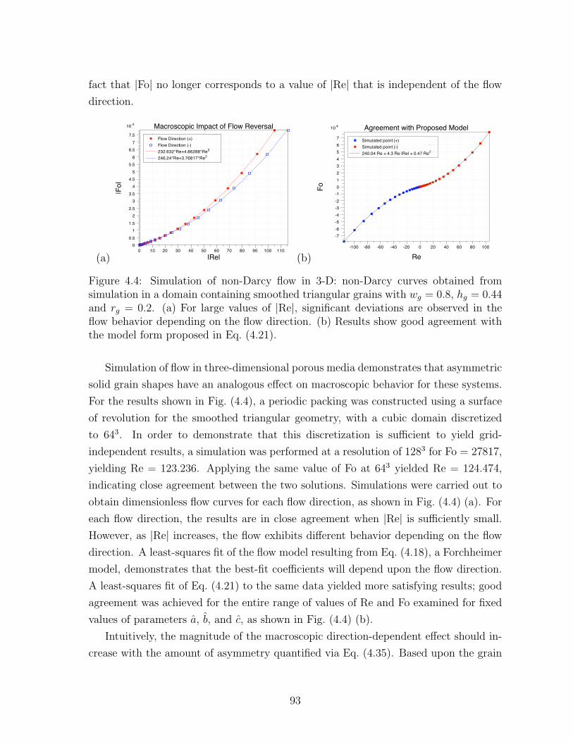
fact that |Fo| no longer corresponds to a value of |Re| that is independent of the flow

direction.

(a)

Flow Direction (+)

Flow Direction (-)

232.632*Re+4.86288*Re2

246.24*Re+3.76817*Re2

0 10 20 30 40 50 60 70 80 90 100 110

104

0

0.5

1

1.5

2

2.5

3

3.5

4

4.5

5

5.5

6

6.5

7

7.5

Macroscopic Impact of Flow Reversal

|Re|

|Fo|

(b)

Simulated point (+)

Simulated point (-)

240.04 Re + 4.3 Re |Re| + 0.47 Re2

-100 -80 -60 -40 -20 0 20 40 60 80 100

104

-7

-6

-5

-4

-3

-2

-1

0

1

2

3

4

5

6

7

Agreement with Proposed Model

Re

Fo

Figure 4.4: Simulation of non-Darcy flow in 3-D: non-Darcy curves obtained fromsimulation in a domain containing smoothed triangular grains with wg = 0.8, hg = 0.44and rg = 0.2. (a) For large values of |Re|, significant deviations are observed in theflow behavior depending on the flow direction. (b) Results show good agreement withthe model form proposed in Eq. (4.21).

Simulation of flow in three-dimensional porous media demonstrates that asymmetric

solid grain shapes have an analogous effect on macroscopic behavior for these systems.

For the results shown in Fig. (4.4), a periodic packing was constructed using a surface

of revolution for the smoothed triangular geometry, with a cubic domain discretized

to 643. In order to demonstrate that this discretization is sufficient to yield grid-

independent results, a simulation was performed at a resolution of 1283 for Fo = 27817,

yielding Re = 123.236. Applying the same value of Fo at 643 yielded Re = 124.474,

indicating close agreement between the two solutions. Simulations were carried out to

obtain dimensionless flow curves for each flow direction, as shown in Fig. (4.4) (a). For

each flow direction, the results are in close agreement when |Re| is sufficiently small.

However, as |Re| increases, the flow exhibits different behavior depending on the flow

direction. A least-squares fit of the flow model resulting from Eq. (4.18), a Forchheimer

model, demonstrates that the best-fit coefficients will depend upon the flow direction.

A least-squares fit of Eq. (4.21) to the same data yielded more satisfying results; good

agreement was achieved for the entire range of values of Re and Fo examined for fixed

values of parameters a, b, and c, as shown in Fig. (4.4) (b).

Intuitively, the magnitude of the macroscopic direction-dependent effect should in-

crease with the amount of asymmetry quantified via Eq. (4.35). Based upon the grain

93

Table 4.1: Properties for asymmetric porous media constituted of solid grains definedby Eq. (4.28)

s rx rd ε Gaxx Ga

rr a b c0.0 0.5 0.5 0.476349 0 0 219.76 3.01295 2.1× 10−17

0.25 0.5 0.499 0.478561 -0.01033 0.00388 217.64 3.4277 -0.067390.5 0.505 0.496 0.48027 -0.02031 0.00765 218.4 3.4041 -0.106540.75 0.51 0.4913 0.484818 -0.02947 0.01118 218.88 3.3987 -0.132881.0 0.52 0.4845 0.489792 -0.03765 0.01434 220.17 3.3462 -0.16671.25 0.54 0.474 0.496414 -0.04474 0.01693 223.26 3.1492 -0.199961.5 0.57 0.4617 0.503387 -0.0499 0.0187 224.85 2.9948 -0.24174

shape described by Eq. (4.28), several periodic media were constructed to illustrate this

correlation, as listed in Table 4.1. The medium asymmetry was controlled by increas-

ing the value of s, and values of rx and rd were chosen in order to preserve a relatively

constant value of the coefficient a, which is proportional to a the inverse of the leading

order term in the permeability. The best-fit parameters a, b and c listed in Table 4.1

were obtained to match simulated data. By construction, the leading-order parameter

a varies only within a narrow range. Of particular interest is the parameter c, which

determines the magnitude of the direction-dependent effect. The data demonstrates

that as asymmetry increases, the magnitude of c will also increase. Since the asymme-

try of the geometry defined by Eq. (4.28) depends on a single parameter, it is sufficient

to express it in terms of Gaxx only. Data listed in Table 4.1 are plotted in Fig. (4.5)

(a), demonstrating a one-to-one relationship between Gaxx and s. Consequently, the

coefficient c can expressed as a function of Gaxx, a quantity which can be computed for

general grain shapes, as opposed to s which is specific to Eq. (4.28).

While this data does not provide a basis for the formulation of a precise param-

eterized closure relation, it does provide strong evidence that extended anisotropic

properties of a particular porous medium can be predicted using the tensor Ga. As

a consequence, the set of morphological measures M should include this quantity in

addition to other quantities likely to influence the macroscopic behavior. The work

performed here suggests that porosity, solid surface area, and orientation tensors are

all likely to have an impact on the flow coefficients a(M), b(M) and c(M).

94

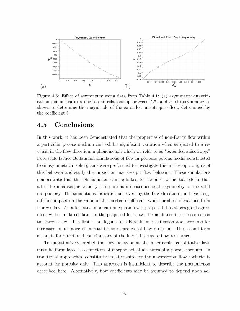
(a)

0 0.2 0.4 0.6 0.8 1 1.2 1.4

-0.045

-0.04

-0.035

-0.03

-0.025

-0.02

-0.015

-0.01

-0.005

0Asymmetry Quantification

s

Ga xx

(b)-0.045 -0.04 -0.035 -0.03 -0.025 -0.02 -0.015 -0.01 -0.005 0

-0.24

-0.22

-0.2

-0.18

-0.16

-0.14

-0.12

-0.1

-0.08

-0.06

-0.04

-0.02

0Directional Effect Due to Asymmetry

Gaxx

ĉ

Figure 4.5: Effect of asymmetry using data from Table 4.1: (a) asymmetry quantifi-cation demonstrates a one-to-one relationship between Ga

xx and s; (b) asymmetry isshown to determine the magnitude of the extended anisotropic effect, determined bythe coefficient c.

4.5 Conclusions

In this work, it has been demonstrated that the properties of non-Darcy flow within

a particular porous medium can exhibit significant variation when subjected to a re-

versal in the flow direction, a phenomenon which we refer to as “extended anisotropy.”

Pore-scale lattice Boltzmann simulations of flow in periodic porous media constructed

from asymmetrical solid grains were performed to investigate the microscopic origins of

this behavior and study the impact on macroscopic flow behavior. These simulations

demonstrate that this phenomenon can be linked to the onset of inertial effects that

alter the microscopic velocity structure as a consequence of asymmetry of the solid

morphology. The simulations indicate that reversing the flow direction can have a sig-

nificant impact on the value of the inertial coefficient, which predicts deviations from

Darcy’s law. An alternative momentum equation was proposed that shows good agree-

ment with simulated data. In the proposed form, two terms determine the correction

to Darcy’s law. The first is analogous to a Forchheimer extension and accounts for

increased importance of inertial terms regardless of flow direction. The second term

accounts for directional contributions of the inertial terms to flow resistance.

To quantitatively predict the flow behavior at the macroscale, constitutive laws

must be formulated as a function of morphological measures of a porous medium. In

traditional approaches, constitutive relationships for the macroscopic flow coefficients

account for porosity only. This approach is insufficient to describe the phenomenon

described here. Alternatively, flow coefficients may be assumed to depend upon ad-

95

ditional morphological properties. Thermodynamically constrained averaging theory

provides some guidance for the determination of these quantities. To treat the case

of extended anisotropy, we construct a tensor that serves as a measure of reflection

asymmetry. Preliminary results show a strong correlation between this quantity and

the strength of the direction-dependent effect.

Examination of non-Darcy flow within the simple, oriented packings considered

in this work provides useful physical insights into the underlying mechanisms that

lead to extended anisotropy. Introduction of a tensor to serve as a measure of solid-

phase asymmetry provides an opportunity to quantitatively evaluate the impact of this

aspect of the solid geometry on macroscopic flow behavior. However, the simple grain

shapes considered in this work do not adequately represent the range of asymmetries

possible in general porous media. Our research indicates that additional quantities,

including porosity, solid surface area, and solid orientation tensors, must be accounted

for in order to adequately predict coefficients for certain anisotropic flows. Many open

questions remain with respect to approximation of morphological properties of real

porous media. Extension of closure relationships to incorporate additional aspects

of porous medium morphology presents an opportunity to more accurately predict

macroscopic flow parameters.

96

Chapter 5

Summary and Recommendations

Microscale simulation plays a vital role in the development of macroscopic porous

medium models. Flow simulations performed for single- and multi- phase systems pro-

vide a clear way to study the macroscopic implications of flow processes, determine the

suitability of modeling assumptions and approximations, and develop macroscopic con-

stitutive laws. Various numerical tools are needed to generate microscopic simulation

results and perform upscaling in a manner consistent with the theoretical framework.

The lattice Boltzmann method is a flexible and widely used for simulating flow pro-

cesses in porous media. The large domain sizes required to study macroscopic processes

necessitate high-performance, parallel implementations of the LBM. In addition to mi-

croscopic flow simulators, geometric analysis tools are required to accurately compute

averaged quantities from microscopic simulation data. The major contributions from

previous chapters of this document are summarized as follows:

• Development of efficient parallel lattice Boltzmann simulators for one- and two-

phase flows in porous media;

• Construction of analysis tools for upscaling simulation results to the macroscale;

• Assessment of computational constraints on porous medium simulations for per-

meability estimation and generation of two-phase equilibrium configurations;

• Analysis of the macroscopic form for the momentum equation for single-phase

flow subject to asymmetrical flow geometry.

This chapter addresses remaining challenges and opportunities for microscale porous

medium simulation. In particular, the ensuing sections focus on problems of particular

interest to the advancement of macroscopic porous media and identifies areas for which

existing tools are insufficient to meet the demands imposed by these problems.

5.1 Single Phase Flow

Single phase flow represents the simplest and most well-established porous medium

modeling scenario. Microscale simulation techniques such as the MRT LBM are capable

of carrying out simulations in realistic porous media based for domain sizes which

approach the REV for homogeneous and moderately heterogeneous media. Macroscopic

descriptions of single phase flows offer reliable predictions for many systems, and a

connection between macroscopic and microscopic physics is well-established [52, 53,

142, 60].

The results of Chapter 5 demonstrate that how microscale simulation can be ex-

tended to gain insight into the functional form of the momentum equation for non-

Darcy flow in porous media. These results demonstrate that the correction to the

Darcy permeability is linear in both the flow velocity and its absolute value, leading

to a correction which depends on both the flow velocity and the flow direction. This

direction dependence can be identified with asymmetry of the flow field which results

from the formation of eddies as determined by the shape of asymmetrical solid grains.

The values of the associated macroscopic flow coefficients can be predicted as a function

of this asymmetry.

In spite of relatively mature understanding of single phase flows, a variety of open

questions remain, particularly with respect to heterogeneous and anisotropic systems.

Extending the predictive capabilities of macroscopic constitutive laws for the perme-

ability and inertial coefficients is a straightforward application of the tools and ideas

presented herein. In Chapter 4, it was suggested that these coefficients can be expressed

generally as functions of a set of dimensionless measures of the solid morphology. Quan-

titative assessments based on the measures of greatest importance would provide useful

extensions to existing correlations which consider these coefficients to be a function of

porosity only. Incorporating orientation tensors into these expressions would provide

a natural measure by which correlations could be extended to consider anisotropic

systems.

5.2 Multiphase Flow

Multiphase flow processes are substantially less well understood in comparison to single

phase flows. Open questions remain at all scales, and the development of computation-

ally tractable and physically realistic microscopic simulation approaches is an important

98

area of ongoing research. Primary objectives of porous medium study are the elucida-

tion of equilibrium and near-equilibrium behavior of multi- fluid systems, including:

• Development of non-hysteretic relationships to describe the equilibrium state for

multi-fluid systems;

• Construction of non-hysteretic relative permeability relationships;

• Evaluation of the range of systems for which equilibrium and near-equilibrium

approximations may be applied;

• Investigation snap-off phenomena for non-wetting phases and identification of

morphology and flow based criteria for snap-off and reconnection on non-wetting

phases.

These research objectives impose specific demands on numerical tools, including both

simulators and morphological analysis tools. While morphological analysis is unlikely

to be a limiting factor in terms of computational time, measurement of certain vari-

ables may still present challenges. Computation of interfacial mean curvatures, for

example, can be accomplished efficiently and accurately for simple test cases, extension

to simulation data is not always straightforward. Most porous medium data sets are

discontinuous at fluid-solid interfaces, posing a problem for the curvature estimates

presented in Chapter 3. Since accurate computation of the average curvature is essen-

tial to the study of capillary pressures, further study of these schemes is necessary to

improve the fidelity of these measurements.

Significant physical and computational hurdles restrict microscale studies of multi-

phase porous medium flows using the LBM. These may be divided into two categories:

(1) physical inaccuracies that result from incorrect description of fluid physics; (2) nu-

merical limitations related to the timescale for flow processes in multiphase systems.

Addressing these issues and developing efficient simulators which adequately represent

multiphase physics is essential for study of porous medium systems. Relatively simple

LB schemes such as the Shan-Chen method are most typically used to perform simu-

lations of flow processes in multiphase porous media. While a wide range of schemes

exist to simulate multiphase flows, only a small subset have been applied to porous

medium systems. More physically accurate description of the fluid interfaces can be

accomplished by considering more sophisticated schemes which deal directly with the

physical deficiencies inherent in the Shan-Chen LBM [84, 86, 85, 100, 96, 172, 173, 82].

The issues of greatest interest are as follows:

99

(1) A widely recognized shortcoming of the Shan-Chen LBM is the non-physical

definition of the fluid velocity near interfaces, which prevents direct computation of

averaged velocities for associated systems. Alternate multiphase schemes have been

constructed which correct for these spurious currents by constructing a consistent dis-

cretization for the interaction potential [147, 36].

(2) In order to properly treat multiphase thermodynamics, solid boundary con-

ditions must be introduced to generate an associated surface energy for each fluid.

A typical approach is to handle solid surface energies with a boundary condition for

the contact angle, which only been devised for a subset of multiphase LB schemes

[102, 81, 106, 196]. Testing for these schemes has only been performed for the most

straightforward solid morphologies and dynamic expressions for the contact angle,

where needed, are not well-established. These issues are of critical importance to the de-

velopment of valid simulation regimes for description of equilibria in multiphase porous

media.

(3) Non-physical dissolution phenomena result from the application of an ideal gas

equation of state within the bulk phases in the Shan-Chen LBM. Alternative schemes

de-couple the pressure and density fields in order to more accurately describe non-ideal

fluids [122]. Evidence suggests that such schemes can be subject to mass conservation

issues and must therefore be treated with caution [82].

(4) Multiphase drainage simulations require long simulation times before fluids reach

equilibrium configurations. These long equilibration times are a consequence of the fact

that the fluid interfaces must migrate through a porous medium until they reach a stable

configuration, a process which is inherently controlled by the flow velocity. Very small

flow velocities push iteration counts into the millions even for relatively small systems.

Since the flow velocity is determined by the solution of a physical problem, the only

ways to reduce the simulation demands are to take a larger timestep or to perform

fewer lattice updates per iteration. The implication is that schemes which utilize grid

refinement are likely to provide a significant advantage with respect to accelerated

simulation of large systems.

100

BIBLIOGRAPHY

[1] B. Ahrenholz, J. Toelke, P. Lehmann, A. Peters, A. Kaestner, M. Krafczyk, and

W. Durner. Prediction of capillary hysteresis in a porous material using lattice-

Boltzmann methods and comparison to experimental data and a morphological

pore network model. ADVANCES IN WATER RESOURCES, 31(9):1151–1173,

SEP 2008.

[2] M. S. Al-Gharbi and M. J. Blunt. Dynamic network modeling of two-phase

drainage in porous media. Physical Review E, 71(1), 2005.

[3] R. I. Al-Raoush and C. S. Willson. Extraction of physically realistic pore network

properties from three-dimensional synchrotron X-ray microtomography images

of unconsolidated porous media systems. Journal of Hydrology, 300(1–4):44–64,

2005.

[4] J. S. Andrade, U. M. S. Costa, M. P. Almeida, H. A. Makse, and H. E. Stanley.

Inertial effects on fluid flow through disordered porous media. Physical Review

Letters, 82(26):5249–5252, 1999.

[5] A. H. M. F. Anwar, M. Bettahar, and U. Matsubayashi. A method for deter-

mining air-water interfacial area in variably saturated porous media. Journal of

Contaminant Hydrology, 43:129–146, 2000.

[6] R. Argentini, A. Bakker, and C. Lowe. Efficiently using memory in lattice Boltz-

mann simulations. Future Generation Computer Systems, 20(6):973–980, 2004.

[7] R Argentini, AF Bakker, and CP Lowe. A reduced-storage implementation of the

lattice Boltzmann equation. In Sloot, MAP and Abramson, D and Bogdanov,

AV and Dongarra, JJ and Zomaya, AY and Gorbachev, YE, editor, COMPU-

TATIONAL SCIENCE - ICCS 2003, PT I, PROCEEDINGS, volume 2657 of

LECTURE NOTES IN COMPUTER SCIENCE, pages 987–996. 2003.

[8] S. Arnout, F. Verhaeghe, B. Blanpain, and P. Wollants. Lattice Boltzmann model

for diffusion-controlled indirect dissolution. COMPUTERS & MATHEMATICS

WITH APPLICATIONS, 55(7):1377–1391, APR 2008.

101

[9] P. Asinari. Semi-implicit-linearized multiple-relaxation-time formulation of lat-

tice Boltzmann schemes for mixture modeling. Physical Review E, 73:056705–1–

056705–24, 2006.

[10] Pietro Asinari. Multiple-relaxation-time lattice Boltzmann scheme for homoge-

neous mixture flows with external force. PHYSICAL REVIEW E, 77(5, Part 2),

MAY 2008.

[11] Pietro Asinari and Li-Shi Luo. A consistent lattice Boltzmann equation with

baroclinic coupling for mixtures. JOURNAL OF COMPUTATIONAL PHYSICS,

227(8):3878–3895, APR 1 2008.

[12] D. G. Avraam and A. C. Payatakes. Flow regimes and relative permeabilities

during steady-state two-phase flow in porous media. Journal of Fluid Mechanics,

293:207–236, 1995.

[13] D. G. Avraam and A. C. Payatakes. Generalized relative permeability coefficients

during steady-state two-phase flow in porous media, and correlation with the flow

mechanisms. Transport in Porous Media, 20(1-2):135–168, 1995.

[14] D. G. Avraam and A. C. Payatakes. Flow mechanisms, relative permeabilities,

and coupling effects in steady-state two-phase flow through porous media, the case

of strong wettability. Industrial and Engineering Chemistry Research, 38(3):778–

786, 1999.

[15] M. Ayub and R. G. Bentsen. Interfacial viscous coupling: A myth or reality?

Journal of Petroleum Science and Engineering, 23(1):13–26, 1999.

[16] J. Bear. Dynamics of Fluids in Porous Media. Elsevier, New York, 1972.

[17] J. Bear. Hydraulics of Groundwater. McGraw-Hill, New York, 1979.

[18] L. S. Bennethum and T. Giorgi. Generalized Forchheimer equation for two-phase

flow based on hybrid mixture theory. Transport in Porous Media, 26(3):261–275,

1997.

[19] M. Bernaschi, S. Melchionna, S. Succi, M. Fyta, E. Kaxiras, and J. K. Sircar.

MUPHY: A parallel MUlti PHYsics/scale code for high performance bio-fluidic

simulations. COMPUTER PHYSICS COMMUNICATIONS, 180(9):1495–1502,

SEP 2009.

102

[20] M. J. Blunt, M. D. Jackson, M. Piri, and P. H. Valvatne. Detailed physics,

predictive capabilities and macroscopic consequences for pore-network models of

multiphase flow. Advances in Water Resources, 25(8-12):1069–1089, 2002.

[21] S. A. Bradford and L. M. Abriola. Dissolution of residual tetrachloroethylene in

fractional wettability porous media: Incorporation of interfacial area estimates.

Water Resources Research, 37(5):1183–1195, 2001.

[22] S. A. Bradford, L. M. Abriola, and K. M. Rathfelder. Flow and entrapment

of dense nonaqueous phase liquids in physically and chemically heterogeneous

aquifer formations. Advances in Water Resources, 22(2):117–132, 1998.

[23] S. A. Bradford and F. J. Leij. Wettability effects on scaling two- and three-fluid

capillary pressure saturation relations. Environmental Science & Technology,

29(6):1446–1455, 1995.

[24] S. A. Bradford and F. J. Leij. Predicting two- and three-fluid capillary pres-

sure saturation relationships of porous media with fractional wettability. Water

Resources Research, 32(2):251–259, 1996.

[25] S. A. Bradford and F. J. Leij. Estimating interfacial areas for multi-fluid soil

systems. Journal of Contaminant Hydrology, 27(1–2):83–105, 1997.

[26] S. A. Bradford, T. J. Phelan, and L. M. Abriola. Dissolution of residual tetra-

chloroethylence in fractional wettability porous media: Correlation development

and application. Journal of Contaminant Hydrology, 45:35–61, 2000.

[27] R. H. Brooks and A. T. Corey. Properties of porous media affecting fluid flow.

Journal of the Irrigation and Drainage Division, Proceedings of the American

Society of Civil Engineers, IR2:61–88, 1966.

[28] S. Bryant and M. Blunt. Prediction of relative permeability in simple porous

media. Physical Review A, 46(4):2004–2011, 1992.

[29] M. A. Celia and P. Binning. A mass conservative numerical solution for two-phase

flow in porous media with application to unsaturated flow. Water Resources

Research, 28(10):2819–2828, 1992.

[30] M. A. Celia, S. M. Hassanizadeh, and H. K. Dahle. Inclusion of dynamic cap-

illary pressure in unsaturated flow simulators. In EOS Transactions, American

103

Geophysical Union Fall Meeting, volume 82(47), pages H12F–02, San Francisco,

CA, 2001. American Geophysical Union.

[31] M. A. Celia, H. Rajaram, and L. A. Ferrand. A multi-scale computational model

for multiphase flow in porous media. Advances in Water Resources, 16(1):81–92,

1993.

[32] M. A. Celia, P. C. Reeves, and L. C. Ferrand. Recent advances in pore

scale models for multiphase flow in porous media. Reviews of Geophysics,

33(Supplement):1049–1057, 1995.

[33] S. Chen and G. D. Doolen. Lattice Boltzmann method for fluid flows. Annual

Review of Fluid Mechanics, 30:329–364, 1998.

[34] Z. X. Chen, S. L. Lyons, and G. Qin. Derivation of the Forchheimer law via

homogenization. Transport in Porous Media, 44(2):325–335, 2001.

[35] J. T. Cheng, L. J. Pyrak-Nolte, D. D. Nolte, and N. J. Giordano. Linking pressure

and saturation through interfacial areas in porous media. Geophysical Research

Letters, 31(8), 2004.

[36] Daniele Chiappini, Gino Bella, Sauro Succi, Federico Toschi, and Stefano Uber-

tini. Improved Lattice Boltzmann Without Parasitic Currents for Rayleigh-Taylor

Instability. COMMUNICATIONS IN COMPUTATIONAL PHYSICS, 7(3):423–

444, MAR 2010.

[37] M. E. Coles, R. D. Hazlett, E. L. Muegge, K. W. Jones, B. Andrews, B. Dowd,

P. Siddons, A. Peskin, P. Spanne, and W. Soll. Developments in synchrotron X-

ray microtomography with applications to flow in porous media. SPE Reservoir

Evaluation and Engineering, 1(4):288–296, 1998.

[38] K. A. Culligan, D. Wildenschild, B. S. B. Christensen, W. G. Gray, M. L.

Rivers, and A. F. B. Tompson. Interfacial area measurements for unsaturated

flow through a porous medium. Water Resources Research, 40(12), 2004.

[39] H. K. Dahle and M. A. Celia. A dynamic network model for two-phase immiscible

flow. Computational Geosciences, 3(1):1–22, 1999.

104

[40] E. Dalla, M. Hilpert, and C. T. Miller. Computation of the interfacial area for two-

fluid porous medium systems. Journal of Contaminant Hydrology, 56(1–2):25–48,

2002.

[41] H. Darcy. Les Fontaines Publiques de la Ville de Dijon. Dalmont, Paris, 1856.

[42] E. Davies. Machine vision: Theory, algorithms, practicalities. Academic Press,

San Diego, 1997.

[43] K. S. Delibasis, G. K. Matsopoulos, N. A. Mouravliansky, and K. S. Nikita. A

novel and efficienet implementation of the marching cubes algorithm. Computer-

ized Medical Imaging and Graphics, 25:343–352, 2001.

[44] D. d’Humieres, I. Ginzburg, M. Krafczyk, P. Lallemand, and L. S. Luo. Multiple-

relaxation-time lattice Boltzmann models in three dimensions. Philosophical

Transactions of the Royal Society of London Series A-Mathematical Physical and

Engineering Sciences, 360:437–451, 2002.

[45] L. A. Dillard and M. J. Blunt. Development of a pore network simulation model to

study nonaqueous phase liquid dissolution. Water Resources Research, 36(2):439–

454, 2000.

[46] L. A. Dillard, H. I. Essaid, and M. J. Blunt. A functional relation for field-

scale nonaqueous phase liquid dissolution developed using a pore network model.

Journal of Contaminant Hydrology, 48:89–119, 2001.

[47] Hang Ding, Peter D. M. Spelt, and Chang Shu. Diffuse interface model for

incompressible two-phase flows with large density ratios. JOURNAL OF COM-

PUTATIONAL PHYSICS, 226(2):2078–2095, OCT 1 2007.

[48] F. A. L. Dullien. Porous Media: Fluid Transport and Pore Structure. Academic

Press, San Diego, CA, 1992.

[49] L. Fan, H. Fang, and Z. Lin. Simulation of contact line dynamics in a two-

dimensional capillary tube by the lattice Boltzmann model. Physical Review E.,

63:051603:1–6, 2001.

[50] Zhe Fan, Feng Qiu, and Arie E. Kaufman. Zippy: A framework for computa-

tion and visualization on a GPU cluster. COMPUTER GRAPHICS FORUM,

27(2):341–350, APR 2008.

105

[51] S. D. Feng, L. H. Zhong, S. T. Gao, and P. Dong. Equilibrium distribution bound-

ary condition in lattice Boltzmann model and numerical simulation of Darcy-

Forchheimer drag for fluid flow across a square cylinder array. Acta Physica

Sinica, 56(3):1238–1244, 2007.

[52] P. H. Forchheimer. Wasserbewegun durch boden. Zeitschrift des Vereines

Deutscher Ingenieure, 45:1782–1788, 1901.

[53] M. Fourar, G. Radilla, R. Lenormand, and C. Moyne. On the non-linear behavior

of a laminar single-phase flow through two and three-dimensional porous media.

Advances in Water Resources, 27(6):669–677, 2004.

[54] I. Ginzburg and D. d’Humieres. Multireflection boundary conditions for lattice

Boltzmann models. Physical Review E, 68:066614:1–30, 2003.

[55] M. Gladkikh and S. Bryant. Prediction of interfacial areas during imbibition in

simple porous media. Advances in Water Resources, 26(6):609–622, 2003.

[56] J. Goetz, K. Iglberger, C. Feichtinger, S. Donath, and U. Ruede. Coupling multi-

body dynamics and computational fluid dynamics on 8192 processor cores. PAR-

ALLEL COMPUTING, 36(2-3):142–151, FEB-MAR 2010.

[57] W. G. Gray and S. M. Hassanizadeh. Macroscale continuum mechanics for multi-

phase porous-media flow including phases, interfaces, common lines and common

points. Advances in Water Resources, 21(4):261–281, 1998.

[58] W. G. Gray and C. T. Miller. Examination of Darcy’s law for flow in porous media

with variable porosity. Environmental Science & Technology, 38(22):5895–5901,

2004.

[59] W. G. Gray and C. T. Miller. Thermodynamically constrained averaging theory

approach for modeling flow and transport phenomena in porous medium systems:

1. Motivation and overview. Advances in Water Resources, 28(2):161–180, 2005.

[60] W. G. Gray and C. T. Miller. Thermodynamically constrained averaging theory

approach for modeling flow and transport phenomena in porous medium systems:

3. Single-fluid-phase flow. Advances in Water Resources, 29(11):1745–1765, 2006.

106

[61] W. G. Gray and C. T. Miller. Thermodynamically constrained averaging theory

approach for heat transport in single-fluid-phase porous media systems. Journal

of Heat Transfer, In press, 2009.

[62] W. G. Gray and C. T. Miller. Thermodynamically constrained averaging theory

approach for modeling flow and transport phenomena in porous medium systems:

5. Single-fluid-phase transport. Advances in Water Resources, 32(5):681–711,

2009.

[63] W. G. Gray and C. T. Miller. Thermodynamically constrained averaging theory

approach for modeling flow and transport phenomena in porous medium systems:

7. Single-phase megascale flow models. In review, 2009.

[64] S. M. Hassanizadeh. Derivation of basic equations of mass transport in porous

media, part 2. Generalized Darcy’s and Fick’s laws. Advances in Water Resources,

9(4):207–222, 1986.

[65] S. M. Hassanizadeh, M. A. Celia, and H. K. Dahle. Dynamic effect in the capillary

pressure-saturation relationship and its impact on unsaturated flow. Vadose Zone

Journal, 1:38–57, 2002.

[66] S. M. Hassanizadeh and W. G. Gray. General conservation equations for multi-

phase systems: 3. Constitutive theory for porous media flow. Advances in Water

Resources, 3(1):25–40, 1980.

[67] S. M. Hassanizadeh and W. G. Gray. High-velocity flow in porous-media. Trans-

port in Porous Media, 2(6):521–531, 1987.

[68] S. M. Hassanizadeh and W. G. Gray. Mechanics and thermodynamics of multi-

phase flow in porous media including interphase boundaries. Advances in Water

Resources, 13(4):169–186, 1990.

[69] S. M. Hassanizadeh and W. G. Gray. Thermodynamic basis of capillary pressure

in porous media. Water Resources Research, 29(10):3389–3405, 1993.

[70] S. M. Hassanizadeh and W. G. Gray. Toward an improved description of the

physics of two-phase flow. Advances in Water Resources, 16(1):53–67, 1993.

107

[71] S. M. Hassanizadeh and W. R. Gray. Reply to comments by Barak on ’High

velocity flow in porous media’ by Hassanizadeh and Gray. Transport in Porous

Media, 3(3):319–321, 1988.

[72] Thomas Hauser and Raymond LeBeau. OPTIMIZATION OF A COMPUTA-

TIONAL FLUID DYNAMICS CODE FOR THE MEMORY HIERARCHY: A

CASE STUDY. INTERNATIONAL JOURNAL OF HIGH PERFORMANCE

COMPUTING APPLICATIONS, 24(3):299–318, AUG 2010.

[73] X. He and L. S. Luo. A priori derivation of the lattice Boltzmann equation.

Physical Review E, 55:R6333–R6336, 1997.

[74] X. Y. He, S. Y. Chen, and R. Y. Zhang. A lattice Boltzmann scheme for incom-

pressible multiphase flow and its application in simulation of Rayleigh-Taylor

instability. Journal of Computational Physics, 152(2):642–663, 1999.

[75] R. J. Held and M. A. Celia. Modeling support of functional relationships between

capillary pressure, saturation, interfacial areas and common lines. Advances in

Water Resources, 24:325–343, 2001.

[76] R. J. Held and M. A. Celia. Pore-scale modeling extension of constitutive relation-

ships in the range of residual saturations. Water Resources Research, 37(1):165–

170, 2001.

[77] Vincent Heuveline, Mathias J. Krause, and Jonas Latt. Towards a hybrid par-

allelization of lattice Boltzmann methods. COMPUTERS & MATHEMATICS

WITH APPLICATIONS, 58(5):1071–1080, SEP 2009.

[78] R. J. Hill, D. L. Koch, and A. J. C. Ladd. The first effects of fluid inertia on

flows in ordered and random arrays of spheres. Journal of Fluid Mechanics,

448:213–241, 2001.

[79] M. Hilpert, J. F. McBride, and C. T. Miller. Investigation of the residual-funicular

nonwetting-phase-saturation relation. Advances in Water Resources, 24(2):157–

177, 2000.

[80] J. W. Hopmans, T. Vogel, and P. D. Koblik. X-ray tomography of soil water

distribution in one-step outflow experiments. Soil Science Society of America

Journal, 56(2):355–362, 1992.

108

[81] Haibo Huang, Daniel T. Thorne, Jr., Marcel G. Schaap, and Michael C. Sukop.

Proposed approximation for contact angles in Shan-and-Chen-type multicompo-

nent multiphase lattice Boltzmann models. PHYSICAL REVIEW E, 76(6, Part

2), DEC 2007.

[82] Haibo Huang, Hongwei Zheng, Xi-yun Lu, and Chang Shu. An evaluation of

a 3D free-energy-based lattice Boltzmann model for multiphase flows with large

density ratio. INTERNATIONAL JOURNAL FOR NUMERICAL METHODS

IN FLUIDS, 63(10):1193–1207, AUG 10 2010.

[83] P. T. Imhoff, M. H. Arthur, and C. T. Miller. Complete dissolution of

trichloroethylene in saturated porous media. Environmental Science & Tech-

nology, 32(16):2417–2424, 1998.

[84] T Inamuro, N Konishi, and F Ogino. A Galilean invariant model of the lattice

Boltzmann method for multiphase fluid flows using free-energy approach. COM-

PUTER PHYSICS COMMUNICATIONS, 129(1-3):32–45, JUL 2000.

[85] T Inamuro, T Ogata, S Tajima, and N Konishi. A lattice Boltzmann method

for incompressible two-phase flows with large density differences. JOURNAL OF

COMPUTATIONAL PHYSICS, 198(2):628–644, AUG 10 2004.

[86] Takaji Inamuro. Lattice Boltzmann methods for viscous fluid flows and for two-

phase fluid flows. FLUID DYNAMICS RESEARCH, 38(9):641–659, SEP 2006.

[87] A. B. S. Jackson, C. T. Miller, and W. G. Gray. Thermodynamically con-

strained averaging theory approach for modeling flow and transport phenomena in

porous medium systems: 6. Two-fluid-phase flow. Advances in Water Resources,

32(6):779–795, 2009.

[88] Namgyun Jeong. Advanced Study About the Permeability for Micro-Porous

Structures Using the Lattice Boltzmann Method. TRANSPORT IN POROUS

MEDIA, 83(2):271–288, JUN 2010.

[89] Namgyun Jeong, Do Hyung Choi, and Ching-Long Lin. Prediction of Darcy-

Forchheimer drag for micro-porous structures of complex geometry using the

lattice Boltzmann method. JOURNAL OF MICROMECHANICS AND MICRO-

ENGINEERING, 16(10):2240–2250, OCT 2006.

109

[90] M. L. Johns and L. F. Gladden. Magnetic resonance imaging study of the dis-

solution kinetics of octanol in porous media. Journal of Colloid and Interface

Science, 210(2):261–270, 1999.

[91] S. Kalliadasis and H. C. Chang. Apparent dynamic contact angle of an advancing

gas-liquid meniscus. Physics of Fluids, 6(1):12–23, 1994.

[92] Qinjun Kang, Peter C. Lichtner, and David R. Janecky. Lattice Boltzmann

Method for Reacting Flows in Porous Media. ADVANCES IN APPLIED MATH-

EMATICS AND MECHANICS, 2(5):545–563, OCT 2010.

[93] Qinjun Kang, Peter C. Lichtner, and Dongxiao Zhang. An improved lattice

Boltzmann model for multicomponent reactive transport in porous media at the

pore scale. WATER RESOURCES RESEARCH, 43(12), NOV 29 2007.

[94] M. V. Karkare and T. Fort. Determination of the air-water interfacial area in wet

”unsaturated” porous media. Langmuir, 12(8):2041–2044, 1996.

[95] Arie Kaufman, Zhe Fan, and Kaloian Petkov. Implementing the lattice Boltz-

mann model on commodity graphics hardware. JOURNAL OF STATISTICAL

MECHANICS-THEORY AND EXPERIMENT, JUN 2009.

[96] E. S. Kikkinides, A. G. Yiotis, M. E. Kainourgiakis, and A. K. Stubos. Thermody-

namic consistency of liquid-gas lattice Boltzmann methods: Interfacial property

issues. PHYSICAL REVIEW E, 78(3, Part 2), SEP 2008.

[97] A. Kuzmin and A. A. Mohamad. Multirange multi-relaxation time Shan-Chen

model with extended equilibrium. COMPUTERS & MATHEMATICS WITH

APPLICATIONS, 59(7):2260–2270, APR 2010.

[98] Frederic Kuznik, Christian Obrecht, Gilles Rusaouen, and Jean-Jacques Roux.

LBM based flow simulation using GPU computing processor. COMPUTERS &

MATHEMATICS WITH APPLICATIONS, 59(7):2380–2392, APR 2010.

[99] P. Lallemand and L. S. Luo. Theory of the lattice Boltzmann method: Disper-

sion, dissipation, isotropy, Galilean invariance, and stability. Physical Review E,

61(6):6546–6562, 2000.

110

[100] T Lee and CL Lin. Pressure evolution lattice-Boltzmann-equation method for

two-phase flow with phase change. PHYSICAL REVIEW E, 67(5, Part 2), MAY

2003.

[101] T Lee and CL Lin. A stable discretization of the lattice Boltzmann equation for

simulation of incompressible two-phase flows at high density ratio. JOURNAL

OF COMPUTATIONAL PHYSICS, 206(1):16–47, JUN 10 2005.

[102] Taehun Lee and Paul F. Fischer. Eliminating parasitic currents in the lattice

Boltzmann equation method for nonideal gases. PHYSICAL REVIEW E, 74(4,

Part 2), OCT 2006.

[103] D. Li and A. W. Neumann. Thermodynamic status of contact angles. In A. W.

Neumann and J. K. Spelt, editors, Applied Surface Thermodynamics, pages 109–

168. Marcel Dekker, New York, 1996.

[104] H. Li, C. Pan, and C. T. Miller. Pore-scale investigation of viscous coupling effects

for two-phase flow in porous media. Physical Review E., 72(2):026705:1–14, 2005.

[105] J. Lindblad. Surface area estimation of digitized planes using weighted local

configurations. In Discrete Geometry for Computer Imagery, Proceedings, volume

2886, pages 348–357. 2003.

[106] Lin Liu and Taehun Lee. WALL FREE ENERGY BASED POLYNOMIAL

BOUNDARY CONDITIONS FOR NON-IDEAL GAS LATTICE BOLTZMANN

EQUATION. INTERNATIONAL JOURNAL OF MODERN PHYSICS C,

20(11):1749–1768, NOV 2009.

[107] S. J. Liu and J. H. Masliyah. Single fluid flow in porous media. Chemical Engi-

neering Communications, 150:653–732, 1996.

[108] W. E. Lorenson and H. E. Cline. Marching cubes: A high resolution 3D surface

construction algorithm. Computer Graphics, 21(4):163–169, 1987.

[109] M. I. Lowry and C. T. Miller. Pore-scale modeling of nonwetting-phase residual

in porous media. CMR News, 1(1):7–9, 1994.

[110] L. Luckner, M. T. van Genuchten, and D. R. Nielsen. A consistent set of para-

metric models for the two-phase flow of immiscible fluids in the subsurface. Water

Resources Research, 25(10):2187–2193, 1989.

111

[111] H. Ma and D. W. Ruth. The microscopic analysis of high Forchheimer number

flow in porous-media. Transport in Porous Media, 13(2):139–160, 1993.

[112] H. Ma and D. W. Ruth. A numerical-analysis of the interfacial drag force for

fluid-flow in porous-media. Transport in Porous Media, 17(1):87–103, 1994.

[113] AID Macnab, G Vahala, L Vahala, J Carter, M Soe, and W Dorland. Non-local

closure and parallel performance of lattice Boltzmann models for some plasma

physics problems. PHYSICA A-STATISTICAL MECHANICS AND ITS AP-

PLICATIONS, 362(1):48–56, MAR 15 2006.

[114] R. S. Maier and R. S. Bernard. Lattice-Boltzmann accuracy in pore-scale flow sim-

ulation. JOURNAL OF COMPUTATIONAL PHYSICS, 229(2):233–255, JAN 20

2010.

[115] R. S. Maier, D. M. Kroll, Y. E. Kutsovsky, H. T. Davis, and R. S. Bernard. Sim-

ulation of flow through bead packs using the lattice Boltzmann method. Physics

of Fluids, 10(1):60–74, 1998.

[116] K. Mattila, J. Hyvaeluoma, J. Timonen, and T. Rossi. Comparison of imple-

mentations of the lattice–Boltzmann method. Computers & Mathematics with

Applications, 55(7):1514–1524, 2008.

[117] Keijo Mattila, Jari Hyvaluoma, Tuomo Rossi, Mats Aspnas, and Jan Westerholm.

An efficient swap algorithm for the lattice Boltzmann method. COMPUTER

PHYSICS COMMUNICATIONS, 176(3):200–210, FEB 1 2007.

[118] M. D. Mazzeo and P. V. Coveney. HemeLB: A high performance parallel lattice-

Boltzmann code for large scale fluid flow in complex geometries. COMPUTER

PHYSICS COMMUNICATIONS, 178(12):894–914, JUN 15 2008.

[119] J. F. McBride and C. T. Miller. Nondestructive measurement of phase fractions

in multiphase porous-media experiments by using X-ray attenuation. CMR News,

1(1):10–13, 1994.

[120] J. F. McBride and C. T. Miller. Development and application of X-ray analysis

methods for multiphase porous media systems. In review, 2002.

112

[121] J. E. McClure, D. Adalsteinsson, C. Pan, W. G. Gray, and C. T. Miller. Approx-

imation of interfacial properties in multiphase porous medium systems. Advances

in Water Resources, 30(3):354–365, 2007.

[122] ME McCracken and J Abraham. Multiple-relaxation-time lattice-Boltzmann

model for multiphase flow. PHYSICAL REVIEW E, 71(3, Part 2), MAR 2005.

[123] J. W. Mercer and R. M. Cohen. A review of immiscible fluids in the subsurface:

Properties, models, characterization and remediation. Journal of Contaminant

Hydrology, 6(2):107–163, 1990.

[124] J. W. Mercer, R. M. Parker, and C. P. Spalding. Site characterization: Use

of site characterization data to select applicable remediation technologies. In

Subsurface Restoration Conference — Third International Conference on Water

Quality Research, pages 26–27, Dallas, TX, 1992. National Center for Ground

Water Research.

[125] C. T. Miller. NAPL entrapment and removal in heterogeneous porous media sys-

tems. In GQ 98. International Conference and Special Seminars on Groundwater

Quality: Remediation and Protection, Tubingen, Germany, 1998.

[126] C. T. Miller and W. G. Gray. Hydrogeological research: Just getting started.

Ground Water, 40(3):224–231, 2002.

[127] C. T. Miller and W. G. Gray. Thermodynamically constrained averaging theory

approach for modeling flow and transport phenomena in porous medium systems:

2. Foundation. Advances in Water Resources, 28(2):181–202, 2005.

[128] C. T. Miller and W. G. Gray. Hydrogeological research, education, and practice:

A path to future contributions. Journal of Hydrologic Engineering, 13(1):7–12,

2008.

[129] C. T. Miller and W. G. Gray. Thermodynamically constrained averaging theory

approach for modeling flow and transport phenomena in porous medium systems:

4. Species transport fundamentals. Advances in Water Resources, 31(3):577–597,

2008.

[130] C. T. Miller and P. T. Imhoff. Formulating models for multiphase flow and

transport in heterogeneous porous media: Challenges and approaches. CMR

News, 2(2):1–6, 1996.

113

[131] J. Myre, S. D. C. Walsh, D. Lilja, and M. O. Saar. Performance analysis of

single-phase, multiphase, and multicomponent lattice-Boltzmann fluid flow simu-

lations on GPU clusters. CONCURRENCY AND COMPUTATION-PRACTICE

& EXPERIENCE, 23(4):332–350, MAR 2011.

[132] G. D. Nadkarni and S. Garoff. An investigation of microscopic aspects of contact

angle hysteresis: Pinning of the contact line on a single defect. Europhysics

Letters, 20(6):523–528, 1992.

[133] Ariel Narvaez, Thomas Zauner, Frank Raischel, Rudolf Hilfer, and Jens Hart-

ing. Quantitative analysis of numerical estimates for the permeability of porous

media from lattice-Boltzmann simulations. JOURNAL OF STATISTICAL

MECHANICS-THEORY AND EXPERIMENT, NOV 2010.

[134] NVIDIA. NVidia CUDA Programming Guide, Version 3.0, 2010.

[135] Leonid Oliker, Andrew Canning, Jonathan Carter, John Shalf, and Stephane

Ethier. Scientific application performance on leading scalar and vector super-

computering platforms. INTERNATIONAL JOURNAL OF HIGH PERFOR-

MANCE COMPUTING APPLICATIONS, 22(1):5–20, SPR 2008.

[136] M. Oostrom, M. D. White, and M. L. Brusseau. Theoretical estimation of free and

entrapped nonwetting-wetting fluid interfacial areas in porous media. Advances

in Water Resources, 24(8):887–898, 2001.

[137] C. Pan, M. Hilpert, and C. T. Miller. Pore-scale modeling of saturated perme-

abilities in random sphere packings. Physical Review E, 64(6):9, 2001.

[138] C. Pan, M. Hilpert, and C. T. Miller. Lattice-Boltzmann simulation of two-phase

flow in porous media. Water Resources Research, 40(1), 2004.

[139] C. Pan, L.-S. Luo, and C. T. Miller. An evaluation of lattice Boltzmann schemes

for porous medium flow simulation. Computers & Fluids, 35(8–9):898–909, 2006.

[140] C. Pan, J. F. Prins, and C. T. Miller. A high-performance lattice Boltzmann im-

plementation to model flow in porous media. Computer Physics Communication,

158(2):89–105, 2004.

114

[141] D. Pan, M. Hilpert, and C. T. Miller. Lattice-Boltzmann simulation of immiscible

two-fluid displacement in porous media. In SIAM Conference on Mathematical

and Computational Issues in the Geosciences, Austin, TX, 2003.

[142] M. Panfilov and M. Fourar. Physical splitting of nonlinear effects in high-velocity

stable flow through porous media. Advances in Water Resources, 29(1):30–41,

2006.

[143] O. A. Plumb and S. Whitaker. Dispersion in heterogeneous porous media 1.

Local volume averaging and large-scale averaging. Water Resources Research,

24(7):913–926, 1988.

[144] O. A. Plumb and S. Whitaker. Dispersion in heterogeneous porous media 2.

Predictions for stratified and two-dimensional spatially periodic systems. Water

Resources Research, 24(7):927–938, 1988.

[145] O. A. Plumb and S. Whitaker. Diffusion, adsorption and dispersion in hetero-

geneous porous media: The method of large-scale averaging. In J. H. Cushman,

editor, Dynamics of Fluids in Hierarchical Porous Meida, pages 149–176. Aca-

demic Press, New York, 1990.

[146] O. A. Plumb and S. Whitaker. Diffusion, adsorption and dispersion in porous

media: Small-scale averaging and local volume averaging. In J. H. Cushman,

editor, Dynamics of Fluids in Hierarchical Porous Meida, pages 97–148. Academic

Press, New York, 1990.

[147] C. M. Pooley and K. Furtado. Eliminating spurious velocities in the free-energy

lattice Boltzmann method. PHYSICAL REVIEW E, 77(4, Part 2), APR 2008.

[148] M. L. Porter, M. G. Schaap, and D. Wildenschild. Comparison of interfacial area

estimates for multiphase flow through porous media using computed microto-

mography and lattice-Boltzmann simulations. Water Resources Research, to be

submitted, 2009.

[149] M. L. Porter, D. Wildenschild, G. P. Grant, and J. I. Gerhard. Investigating

nonwetting-wetting phase specic interfacial area in an NAPL-water-glass bead

system using computed microtomography data. Water Resources Research, to be

submitted, 2009.

115

[150] M. L. Porter, D. Wildenschild, and M. G. Schaap. Investigating dynamic behavior

in experimental capillary pressure-saturation curves using a lattice-Boltzmann

model. Eos Trans. AGU, Fall Meet. Suppl., 86(52), 2005.

[151] M. Quintard, H. Bertin, and S. Whitaker. Two-phase flow in heterogeneous

porous media: Large-scale capillary pressure and permeability determination. In

P. R. e. King, editor, The Mathematics of Oil Recovery, pages 751–765. Clarendon

Press, Oxford, 1992.

[152] M. Quintard and S. Whitaker. Transport in chemically and mechanically het-

erogeneous porous media. I: Theoretical development of region-averaged equa-

tions for slightly compressible single-phase flow. Advances in Water Resources,

19(1):29–47, 1996.

[153] M. Quintard and S. Whitaker. Transport in chemically and mechanically hetero-

geneous porous media. II: Comparison with numerical experiments for slightly

compressible single-phase flow. Advances in Water Resources, 19(1):49–60, 1996.

[154] H. Rajaram, L. A. Ferrand, and M. A. Celia. Prediction of relative permeabil-

ity for unconsolidated soils using pore-sale network models. Water Resources

Research, 33(1):43–52, 1997.

[155] P. C. Reeves and M. A. Celia. A functional relationship between capillary pres-

sure, saturation, and interfacial area as revealed by a pore-scale network model.

Water Resources Research, 32(8):2345–2358, 1996.

[156] S. Roll, A. Haase, and M. Vonkienlin. Fast generation of leakproof surfaces from

well-defined objects by a modified marching cubes algorithm. Computer Graphics

Forum, 14(2):127–138, 1995.

[157] K. P. Saripalli, H. Kim, P. S. C. Rao, and M. D. Annable. Measurement of specific

fluid-fluid interfacial areas of immiscible fluids in porous media. Environmental

Science & Technology, 31(3):932–936, 1997.

[158] K. P. Saripalli, P. S. C. Rao, and M. D. Annable. Determination of specific NAPL-

water interfacial areas of residual NAPLs in porous media using the interfacial

tracers technique. Journal of Contaminant Hydrology, 31(3–4):375–391, 1998.

116

[159] M. G. Schaap, M. L. Porter, B. S. B. Christensen, and D. Wildenschild. Com-

parison of pressure-saturation characteristics derived from computed tomography

and lattice Boltzmann simulations. Water Resources Research, 43, 2007.

[160] C. E. Schaefer, D. A. Diarlo, and M. J. Blunt. Experimental measurement of air-

water interfacial area during gravity drainage and secondary imbibition in porous

media. Water Resources Research, 36(4):885–890, 2000.

[161] Claudio Schepke, Nicolas Maillard, and Philippe O. A. Navaux. Parallel Lattice

Boltzmann Method with Blocked Partitioning. INTERNATIONAL JOURNAL

OF PARALLEL PROGRAMMING, 37(6, Sp. Iss. SI):593–611, DEC 2009.

[162] G. Schnaar and M. L. Brusseau. Pore-scale characterization of organic immiscible-

liquid morphology in natural porous media using synchrotron X-ray microtomog-

raphy. Environmental Science & Technology, 39(21):8403–8410, 2005.

[163] W. E. Soll, M. A. Celia, and J. L. Wilson. Micromodel studies of three-fluid porous

media systems: Pore-scale processes relating to capillary pressure-saturation re-

lationships. Water Resources Research, 29(9):2963–2974, 1993.

[164] M. L. Stewart, A. L. Ward, and D. R. Rector. A study of pore geometry effects on

anisotropy in hydraulic permeability using the lattice-Boltzmann method. AD-

VANCES IN WATER RESOURCES, 29(9):1328–1340, SEP 2006.

[165] Kevin Stratford and Ignacio Pagonabarraga. Parallel simulation of particle sus-

pensions with the lattice Boltzmann method. COMPUTERS & MATHEMATICS

WITH APPLICATIONS, 55(7):1585–1593, APR 2008.

[166] Triantafyllos Stylianopoulos, Andrew Yeckel, Jeffrey J. Derby, Xiao-Juan Luo,

Mark S. Shephard, Edward A. Sander, and Victor H. Barocas. Permeability

calculations in three-dimensional isotropic and oriented fiber networks. PHYSICS

OF FLUIDS, 20(12), DEC 2008.

[167] M. C. Sukop, H. Huang, C. L. Lin, M. D. Deo, K. Oh, and J. D. Miller. Distribu-

tion of multiphase fluids in porous media: Comparison between lattice Boltzmann

modeling and micro-x-ray tomography. Physical Review E, 77(2), 2008.

[168] Michael C. Sukop, Haibo Huang, Chen Luh Lin, Milind D. Deo, Kyeongseok Oh,

and Jan D. Miller. Distribution of multiphase fluids in porous media: Comparison

117

between lattice Boltzmann modeling and micro-x-ray tomography. PHYSICAL

REVIEW E, 77(2, Part 2), FEB 2008.

[169] C. Shyam Sunder, G. Baskar, V. Babu, and David Strenski. A detailed perfor-

mance analysis of the interpolation supplemented lattice Boltzmann method on

the Cray T3E and Cray X1. INTERNATIONAL JOURNAL OF HIGH PER-

FORMANCE COMPUTING APPLICATIONS, 20(4):557–570, WIN 2006.

[170] P. S. Swain and R. Lipowsky. Contact angles on heterogeneous surfaces: A new

look at Cassie’s and Wenzel’s laws. Langmuir, 14:6772–6780, 1998.

[171] F. Thauvin and K. K. Mohanty. Network modeling of non-Darcy flow through

porous media. Transport in Porous Media, 31(1):19–37, 1998.

[172] G. Thoemmes, J. Becker, M. Junk, A. K. Vaikuntam, D. Kehrwald, A. Klar,

K. Steiner, and A. Wiegmann. A lattice Boltzmann method for immiscible mul-

tiphase flow simulations using the level set method. JOURNAL OF COMPUTA-

TIONAL PHYSICS, 228(4):1139–1156, MAR 1 2009.

[173] A. Tiribocchi, N. Stella, G. Gonnella, and A. Lamura. Hybrid lattice Boltzmann

model for binary fluid mixtures. PHYSICAL REVIEW E, 80(2, Part 2), AUG

2009.

[174] J. Toelke and M. Krafczyk. TeraFLOP computing on a desktop PC with GPUs

for 3D CFD. INTERNATIONAL JOURNAL OF COMPUTATIONAL FLUID

DYNAMICS, 22(7):443–456, 2008.

[175] J. Tolke, X. Krafczyk, M. Schulz, and E. Rank. Lattice Boltzmann simulations

of binary fluid flow through porous media. Philosophical Transactions of the

Royal Society of London Series A-Mathematical Physical and Engineering Sci-

ences, 360(1792):535–545, 2002.

[176] M. T. van Genuchten. A closed-form equation for predicting the hydraulic conduc-

tivity of unsaturated soils. Soil Science Society of America Journal, 44:892–898,

1980.

[177] AC Velivelli and KM Bryden. Parallel performance and accuracy of lattice

Boltzmann and traditional finite difference methods for solving the unsteady

two-dimensional Burger’s equation. PHYSICA A-STATISTICAL MECHANICS

AND ITS APPLICATIONS, 362(1):139–145, MAR 15 2006.

118

[178] F Verhaeghe, S Arnout, B Blanpain, and P Wollants. Lattice-Boltzmann mod-

eling of dissolution phenomena. PHYSICAL REVIEW E, 73(3, Part 2), MAR

2006.

[179] David Vidal, Robert Roy, and Francois Bertrand. A parallel workload balanced

and memory efficient lattice-Boltzmann algorithm with single unit BGK relax-

ation time for laminar Newtonian flows. COMPUTERS & FLUIDS, 39(8):1411–

1423, SEP 2010.

[180] Stuart D. C. Walsh, Martin O. Saar, Peter Bailey, and David J. Lija. Accelerating

geoscience and engineering system simulations on graphics hardware. COMPUT-

ERS & GEOSCIENCES, 35(12):2353–2364, DEC 2009.

[181] Junye Wang, Xiaoxian Zhang, Anthony G. Bengough, and John W. Crawford.

Performance evaluation of the cell-based algorithms for domain decomposition in

flow simulation. INTERNATIONAL JOURNAL OF NUMERICAL METHODS

FOR HEAT & FLUID FLOW, 18(5-6):656–672, 2008.

[182] JY Wang, XX Zhang, AG Bengough, and JW Crawford. Domain-decomposition

method for parallel lattice Boltzmann simulation of incompressible flow in porous

media. PHYSICAL REVIEW E, 72(1, Part 2), JUL 2005.

[183] G. Wellein, T. Zeiser, G. Hager, and S. Donath. On the single processor perfor-

mance of simple Lattice Boltzmann kernels. Computers and Fluids, 35(8–9):910–

919, 2006.

[184] S. Whitaker. Flow in porous media I: A theoretical derivation of Darcy’s law.

Transport in Porous Media, 1:3–25, 1986.

[185] S. Whitaker. The Forchheimer equation: A theoretical development. Transport

in Porous Media, 25(1):27–61, 1996.

[186] S. Whitaker. Volume averaging of transport equations. In J. P. du Plessis,

editor, Fluid Transport in Porous Media, pages 1–60. Computational Mechanics

Publications, Southampton, 1997.

[187] S. Whitaker. The method of volume averaging. In J. Bear, editor, Theory and

Application of Transport in Porous Media. Kluwer, Dordrecht, Netherlands, 1998.

119

[188] D. Wildenschild, B. S. B. Christensen, J. W. Hopmans, A. J. R. Kent, and

M. L. Rivers. Quantifying pore scale flow processes with X-ray microtomography.

Technical report, 2001.

[189] D. Wildenschild, K. A. Culligan, and B. S. B. Christensen. Application of X-ray

microtomography to environmental fluid flow problems. Developments in X-Ray

Tomography IV, 5535:432–441, 2004.

[190] D. Wildenschild, J. W. Hopmans, M. L. Rivers, and A. J. R. Kent. Quantitative

analysis of flow processes in a sand using synchrotron-based X-ray microtomog-

raphy. Vadose Zone Journal, 4(1):112–126, 2005.

[191] D. Wildenschild, J. W. Hopmans, C. M. P. Vaz, and M. L. Rivers. Advanced

photon source activity report 2000. In Using X-ray microtomography to de-

termine gas and liquid phase distributions in porous media, page available at

http://www.aps.anl.gov/apsar2000/wildenschild1.pdf. Advanced Photon Source,

Argonne National Laboratory, Argonne, IL, 2000.

[192] D. Wildenschild, J. W. Hopmans, C. M. P. Vaz, M. L. Rivers, D. Rikard, and

B. S. B. Christensen. Using X-ray computed tomography in hydrology: Systems,

resolutions, and limitations. Journal of Hydrology, 267(3-4):285–297, 2002.

[193] J Wilke, T Pohl, M Kowarschik, and U Rude. Cache performance optimiza-

tions for parallel lattice Boltzmann codes. In Kosch, H and Boszormenyi, L

and Hellwagner, H, editor, EURO-PAR 2003 PARALLEL PROCESSING, PRO-

CEEDINGS, volume 2790 of LECTURE NOTES IN COMPUTER SCIENCE,

pages 441–450. 2003.

[194] SR Williams and AP Philipse. Random packings of spheres and spherocylinders

simulated by mechanical contraction. PHYSICAL REVIEW E, 67(5, Part 1),

MAY 2003.

[195] J. L. Wilson, S. H. Conrad, W. R. Mason, W. Peplinksi, and E. Hagan. Lab-

oratory investigation of residual organics from spills, leaks, and the disposal of

hazardous wastes in groundwater. Technical Report EPA CR-813571-01-0, U.S.

Environmental Protection Agency, Robert S. Kerr Environmental Research Lab-

oratory, Ada, OK, 1989.

120

[196] Fabiano G. Wolf, Luis O. E. dos Santos, and Paulo C. Philippi. Modeling and sim-

ulation of the fluid-solid interaction in wetting. JOURNAL OF STATISTICAL

MECHANICS-THEORY AND EXPERIMENT, JUN 2009.

[197] S. C. T. Yu. Transport and fate of chlorinated hydrocarbons in the vadose zone—

a literature review with discussions on regulatory implications. Journal of Soil

Contamination, 4(1):25–56, 1995.

[198] T. Zeiser, G. Wellein, A. Nitsure, K. Iglberger, U. Ruede, and G. Hager. In-

troducing a parallel cache oblivious blocking approach for the lattice Boltzmann

method. PROGRESS IN COMPUTATIONAL FLUID DYNAMICS, 8(1-4):179–

188, 2008.

[199] C. Zhou, R. Shu, and M. S. Kankanhalli. Selectively meshed surface representa-

tion. Computer Graphics, 19(6):793–804, 1995.

[200] Q. Zou and X. He. On pressure and velocity boundary conditions for the lattice

Boltzmann BGK model. Physics of Fluids, 9(6):1591–1598, 1997.

121