engineering microscale magnetic devices for next-generation

ENGINEERING MICROSCALE MAGNETIC DEVICES FOR NEXT-GENERATION MICROROBOTICS

By

CAMILO VELEZ CUERVO

A DISSERTATION PRESENTED TO

THE GRADUATE SCHOOL OF THE UNIVERSITY OF FLORIDA IN PARTIAL FULFILLMENT OF THE REQUIREMENTS FOR THE DEGREE OF

DOCTOR OF PHILOSOPHY

UNIVERSITY OF FLORIDA

2017

To my parents, the real reason all this is possible

4

ACKNOWLEDGMENTS

I gratefully thank the guidance, support, and mentorship from my great advisor,

Professor David Arnold. He is the vision of the team and the direction of this work. I

thank my committee members Drs. Jon Dobson, Carlos Rinaldi and Jack Judy. I

specially thank my partners and friends at lab: Dr. Alexandra Garraud, Nicolas Garraud,

Xiao Wen, Keisha Castillo, Yuzheng Wang and the old crew: Drs William Patterson,

Oniku Ololade, Shashank Sawant, Rob Carrol and Bin Qi. Thanks to all Professors and

colleagues at IMG. Very special thanks to the staff of University of Florida’s Research

Service Centers (RSC) at the Herbert Wertheim College of Engineering. I also thanks

colleagues and friends from UF Dr. Isaac Torres-Díaz, Lorena Maldonado-Camargo, Dr.

Fan Ren and David Whitney. And external colleagues: Drs. Ron Pelrine, Annjoe Wong-

Foy, and Allen Hsu at SRI International, Dr. Jonas Henricksson from Femto-Tools AG

and Dr. Johann Osma and German Yamhure for given me the opportunity to mentor

future engineers.

I want to acknowledge funding support from the Defense Advanced Research

Project Agency (DARPA) under AFRL Contract #FA8650-15-C-7547 (the views,

opinions and/or findings expressed are those of the author and should not be

interpreted as representing the official views or policies of the Department of Defense or

the U.S. Government) and the University of Florida Office of Research.

Finally, thanks for the support from my family and Alicia Otálora, Carlos Escobar

(many ideas were born with them), el Corillo (Specially Veronica Negron), Diana

Escobar and Diana Shao and all my friends at Gainesville.

5

TABLE OF CONTENTS

page

ACKNOWLEDGMENTS .................................................................................................. 4

LIST OF TABLES ............................................................................................................ 8

LIST OF FIGURES .......................................................................................................... 9

LIST OF ABBREVIATIONS ........................................................................................... 15

TERMS AND SYMBOLS ............................................................................................... 16

ABSTRACT ................................................................................................................... 18

CHAPTER

1 INTRODUCTION .................................................................................................... 21

1.1 Purpose & Objectives .................................................................................... 24 1.1.1 Research Purpose .............................................................................. 24 1.1.2 Research Objectives ........................................................................... 26

1.1.3 Research Methodology ....................................................................... 27 1.2 Dissertation Overview ................................................................................... 28

2 BACKGROUND ...................................................................................................... 31

2.1 Microrobotics ................................................................................................. 32

2.1.1 Books About Microrobotics ................................................................. 34 2.1.2 Review Papers in Microrobotics .......................................................... 40

2.2 Understanding Magnetostatics ...................................................................... 41

2.2.1 Classification of Magnetic Materials .................................................... 41 2.2.2 Magnetic Model of Ferromagnetic Materials ....................................... 47

2.2.3 Demagnetization Corrections for Ferromagnetic Materials ................. 51 2.2.4 DC Demagnetization (DCD) ................................................................ 55 2.2.5 Stray Magnetic Field Characterization ................................................ 57

2.2.6 Single Magnet Simulation ................................................................... 60 2.2.7 Magnetic Pole Boundary Simulation ................................................... 64 2.2.8 Checkerboard Pattern Simulation ....................................................... 66

2.3 Summary ....................................................................................................... 68

3 MAGNETIC FORCES AT SMALL SCALE .............................................................. 69

3.1 Relevant Forces for Microrobotics ................................................................. 69 3.1.1 Forces Interacting at Long Ranges ..................................................... 70 3.1.2 Surface and Contact Forces ............................................................... 72

6

3.1.3 Hydrodynamic Forces ......................................................................... 74 3.1.4 Actuation Forces ................................................................................. 76

3.2 Theoretical Analysis of the Magnetic Forces ................................................. 77

3.2.1 General Expression for the Magnetic Force ........................................ 78 3.2.2 Specific Cases for the Magnetic Force ................................................ 81

3.3 Analytical Solution of the Force Between Two Magnets ............................... 84 3.4 Diamagnetic Levitation .................................................................................. 86 3.5 Direct Measurement and Microscale Mapping of NanoNewton to

MilliNewton Magnetic Forces ............................................................................... 92 3.5.1 Measuring Magnetic Forces at Microscale .......................................... 93 3.5.2 Experimental ....................................................................................... 94 3.5.3 Results and Discussion ....................................................................... 97

3.6 Summary ..................................................................................................... 100

4 SELECTIVE MAGNETIZATION ............................................................................ 102

4.1 Patterning Magnetic Fields .......................................................................... 102 4.2 Selective Magnetization Process ................................................................ 109

4.2.1 COMSOL Simulation ......................................................................... 110 4.2.2 Magnetization Mask Machining and Model Validation ....................... 113 4.2.3 Variations on the Selective Magnetization ........................................ 115

4.3 Summary ..................................................................................................... 118

5 MICROROBOT FABRICATION: BOTTOM-UP APPROACH ................................ 119

5.1 Magnetic Assembly and Cross-Linking of Nanoparticles for Releasable Magnetic Microstructures ................................................................................... 120

5.2 Results and Discussion ............................................................................... 124 5.3 Experimental Methods ................................................................................ 133

5.3.1 Magnetization Mask Fabrication ....................................................... 133

5.3.2 Substrate Magnetization ................................................................... 135 5.3.3 Nanoparticle Synthesis and Phase Transfer ..................................... 135

5.3.4 Nanoparticle Assembly ..................................................................... 137 5.3.5 Analysis of Nanoparticle Assemblies ................................................ 137 5.3.6 Nanoparticle Crosslinking ................................................................. 138

5.3.7 Structure Release ............................................................................. 138 5.4 Summary ..................................................................................................... 139

6 MICROROBOT FABRICATION: TOP-DOWN APPROACH ................................. 140

6.1 The Magnetic Substrate .............................................................................. 142

6.2 Machining the Magnetic Substrate .............................................................. 146 6.3 Adapting Selective Magnetization for Microrobot Bases ............................. 150

6.3.1 Improving Magnetization: Simulations ............................................... 151 6.3.2 Improving Magnetization: Field Selection .......................................... 154

6.4 The Magnetization Mask ............................................................................. 155 6.4.1 Mask Fabrication Exploration ............................................................ 155

7

6.4.2 Low Aspect Ratio Magnetization Mask ............................................. 158 6.4.3 High Aspect Ratio Magnetization Mask ............................................. 159

6.5 Characterization of Microrobot Bases ......................................................... 163

6.6 Summary ..................................................................................................... 170

7 ADDING FUNCTIONALITY TO MICROROBOTS: END EFFECTORS ................ 171

7.1 End-effector Design and Fabrication ........................................................... 173 7.1.1 Design Considerations ...................................................................... 173 7.1.2 Fabrication ........................................................................................ 175

7.2 Fabrication Results ..................................................................................... 180 7.2.1 Magnetic Attachment and (Lack Of) Self-alignment .......................... 180 7.2.2 Supporting Tethers and Sacrificial Layer .......................................... 182

7.2.3 End Effector Materials ....................................................................... 183 7.2.4 End Effector Tips............................................................................... 184

7.3 End Effector Testing .................................................................................... 186

7.4 Summary ..................................................................................................... 190

8 ADDING FUNCTIONALITY TO MICROROBOTS: ELECTROPERMANENT MAGNETS ............................................................................................................ 192

8.1 Electropermanent Magnet ........................................................................... 193 8.2 Sub-millimeter Electropermanent Magnets for Microgripper ....................... 195

8.2.1 Experimental Results ........................................................................ 196 8.2.2 Simulation Results ............................................................................ 198

8.3 Axisymmetric Sub-millimeter Electropermanent Magnet ............................. 202 8.3.1 Simulations of the Axisymmetric EPM ............................................... 202

8.3.2 Fabrication of the Axisymmetric EPM ............................................... 204 8.3.3 Characterization of the Axisymmetric EPM ....................................... 205

8.4 Summary ..................................................................................................... 209

9 CONCLUSIONS ................................................................................................... 210

9.1 Summary of Research Contributions .......................................................... 210

9.2 Future Work ................................................................................................ 212 9.2.1 Selective Magnetization .................................................................... 213 9.2.2 End Effectors .................................................................................... 216

9.3 Final Conclusions ........................................................................................ 217

REFERENCES ............................................................................................................ 220

BIOGRAPHICAL SKETCH .......................................................................................... 239

8

LIST OF TABLES

Table page 2-1 Magnetic properties of some commercial soft ferromagnetic materials. ............. 46

3-1 Comparison of actuation forces. ......................................................................... 77

7-1 End effector material properties. ....................................................................... 173

7-2 Thickness measurement of each material in the end effector. ......................... 183

9

LIST OF FIGURES

Figure page 1-1 Global robotics industry. ..................................................................................... 21

1-2 Potential global markets for microrobotics .......................................................... 23

1-3 NSF awarded grants for microrobotics. .............................................................. 24

1-4 Selective magnetization concept. ....................................................................... 26

1-5 Modeling methodology concept diagram ............................................................ 28

1-6 Research and document description. ................................................................. 30

2-1 Genealogy tree for microrobotics ........................................................................ 34

2-2 History of publications related with microrobotics ............................................... 34

2-3 Periodic table of elements illustrating their magnetic behavior at 273K .............. 43

2-4 Measured magnetization curves of different types of magnetic materials .......... 46

2-5 Material properties comparison for some soft ferromagnets ............................... 47

2-6 Coordinate system for the calculation of the magnetic field in a point P ............. 49

2-7 Experiment to validate the simulation model of a spherical magnet ................... 51

2-8 Coordinate system representation used to calculate the demagnetization ......... 54

2-9 Example of demagnetization correction .............................................................. 55

2-10 Schematic of the DC demagnetization measurement procedure........................ 56

2-11 DCD in plane and out of plane of an example material ...................................... 57

2-12 State of the art of submillimeter magnetic field measurement techniques .......... 58

2-13 Magneto optical imaging (MOI) measurement technique ................................... 59

2-14 Scanning hall probe measurement technique..................................................... 59

2-15 NdFeB magnet characterization ......................................................................... 60

2-16 Analytical solution of the Bz field produced by a bar magnet .............................. 61

2-17 Magneto optical images of a single NdFeB magnet at different heights ............. 62

10

2-18 Stray magnetic Bz field measurements using magneto optical images ............... 63

2-19 Bx, By and Bz reconstructions from single axis magneto optical images ........... 64

2-20 Magnetic properties of the substrate measured using VSM ............................... 65

2-21 Finite element simulation of the magnetic field generated by the tape ............... 66

2-22 Analytical solution of the Bz produced by a checkerboard pattern ...................... 67

2-23 Comparison between COMSOL simulation (using magnetization curve) ........... 67

3-1 Scaling analysis for forces interacting at long range ........................................... 72

3-2 Scaling analysis for surface forces ..................................................................... 73

3-3 Scaling analysis for hydrodynamic forces ........................................................... 76

3-4 Interpretation of the magnetic force and magnetic torque at microscale ............ 81

3-5 Magnetic force expressions based on the behavior ............................................ 84

3-6 Analytical solution for the force between two cuboidal magnets ......................... 85

3-7 3D representation of the analytical solution for the magnetic force .................... 86

3-8 Stray magnetic field of an array of magnets ....................................................... 89

3-9 Analytical solution to calculate the diamagnetic force ......................................... 90

3-10 Representation of the magnetic force density .................................................... 92

3-11 Direct magnetic force measurement mechanism ................................................ 95

3-12 Micromagnet characterization............................................................................. 95

3-13 Magneto-optical image measurements of the magnetic field (Bz) ....................... 96

3-14 Force measurements at a different scan height above the test sample. ............. 98

3-15 Comparison of analytical model and force measurements ................................. 99

3-16 Magnetic field gradient limits detected by the proposed technique................... 100

4-1 Three different types of permanent magnet power generation technology ....... 104

4-2 First magnetization mechanism by passing current .......................................... 105

4-3 Schematic diagrams of the thermomagnetic patterning process ...................... 107

11

4-4 Sketch of the irradiation induced intermixing .................................................... 108

4-5 Schematic of selective magnetization process ................................................. 110

4-6 Selective magnetization process simulation ..................................................... 111

4-7 Simulations of the stray magnetic field comparison at 50 µm ........................... 112

4-8 Low aspect ratio magnetization mask ............................................................... 113

4-9 Magneto-optical images of the selectively magnetized sample ........................ 114

4-10 Measurement/simulations at 50 μm above the substrate ................................. 115

4-11 Zero-base magnetization experiment description ............................................. 116

4-12 Zero-base magnetization experiment.. ............................................................. 117

4-13 Inclusion of a soft magnetic back plate during the magnetization ..................... 117

4-14 Comparison between manually assembled micro-robot ................................... 118

5-1 A method is presented to batch-fabricate magnetic microstructures ................ 120

5-2 Schematic of fabrication process ...................................................................... 124

5-3 Magnetically assembled iron oxide nanoparticles............................................. 127

5-4 Time dependence of the line height for different volume fractions.................... 128

5-5 Calculation of number of particles per cross section versus time ..................... 129

5-6 Number of particles per unit of length ............................................................... 129

5-7 Schematic of the crosslinking process on iron oxide nanoparticles .................. 131

5-8 Examples of released structures free-floating in water ..................................... 131

5-9 Superimposed snap-shots of a single microstructure translated ...................... 132

5-10 Rotation of a microstructure by rotating the magnetic field (TOP) .................... 133

5-11 Microfabrication process for the selective magnetization mask ........................ 134

6-1 Diamagnetic levitated robots ............................................................................ 141

6-2 Bz field magneto optical image measurement of a 2x2 magnets array ............. 142

6-3 Comparison off magnetic properties commercial available thin film ................. 143

12

6-4 Magnetic characterization comparison for SRI and BJA magnets .................... 144

6-5 Magnetization characterization at different temperatures ................................. 145

6-6 DCD at different temperatures .......................................................................... 146

6-7 Successful dicing of the BJA NdFeB material................................................... 147

6-8 Sample comparison before and after polishing................................................. 148

6-9 Optical microscopy image of the BJA magnet surface ..................................... 149

6-10 Optical profilometer image of polished and unpolished magnet ....................... 150

6-11 Set of materials to take into consideration for the magnetization mask ............ 152

6-12 Selective magnetization simulation model ........................................................ 153

6-13 Selective magnetization simulation model, double mask .................................. 154

6-14 DC magnetization of lines, varying the applied magnetic field. ......................... 155

6-15 (Top) Mask fabrication initial exploration with a batch of four robots per mask 156

6-16 Magneto optical images measured at 50 µm .................................................... 157

6-17 Modeling the log aspect ratio mask .................................................................. 158

6-18 Model and fabrication of double side mask ...................................................... 159

6-19 Laminated mask approach ............................................................................... 160

6-20 Finding the right external magnetic field ........................................................... 161

6-21 Magneto optical image of a selectively magnetized samples ........................... 162

6-22 3D simulation of the laminated mask (double mask) ........................................ 163

6-23 Magneto optical image of the selective magnetization of BJA substrates ........ 164

6-24 MOI measures .................................................................................................. 165

6-25 Fabrication of nine micro-robots per batch ....................................................... 166

6-26 MOI characterization of samples from the same batch (280 µm thickness) ..... 166

6-27 Scanning hall probe measurements ................................................................. 167

6-28 Diamagnetic force measurement using a microbalance ................................... 169

13

6-29 Characterization of batch fabricated robots at SRI ........................................... 169

7-1 Comparison between fabricated end effector ................................................... 172

7-2 Microfabricated end effector assembled on a magnetic base ........................... 175

7-3 Cross section schematic and layer thicknesses ............................................... 176

7-4 End effector fabrication schematics .................................................................. 178

7-5 Fabrication recipe for hybrid (Nickel + SU-8) end effector ................................ 179

7-6 Fabrication recipe for hybrid (Nickel + SU-8) end effector ................................ 180

7-7 Three designs of magnetic attachment to the magnetic base .......................... 181

7-8 End effectors assembly tests ............................................................................ 182

7-9 Examples of end effectors fabricated in the second generation ....................... 183

7-10 Released end effectors fabricated in four different techniques ......................... 184

7-11 Fabrication of different tools and resolutions .................................................... 185

7-12 Three examples of end effector tips made in nickel .......................................... 185

7-13 Hybrid end effector tips made of nickel and SU-8 ............................................. 186

7-14 Top view of nickel end effector mounted on magnetic bases ........................... 187

7-15 Pick and place testing using end effectors coated with SBS ............................ 188

7-16 Sequence of the end effector entering and leaving a droplet ........................... 189

7-17 Sequence demonstrating the proof of concept of µEDM .................................. 190

8-1 Concept of switchable magnets. ....................................................................... 193

8-2 Concept of electropermanent magnet .............................................................. 194

8-3 EPM schematics. A)EPM configurations in the on/off states ............................ 196

8-4 Magnetic field measurements for EPM fabricated with two materials ............... 198

8-5 NdFeB 1500 µm x 2000 µm x 500 µm EPM magnetic field .............................. 199

8-6 COMSOL simulation results for a NdFeB EPM ................................................ 200

8-7 Simulation of the beam stress and deflection when the EPM is “on”. ............... 201

14

8-8 Operational concept of the conventional and new axisymmetric EPM ............. 202

8-9 Example EPM configuration yielding maximum latching force on/off ratio ........ 203

8-10 2D axisymmetric COMSOL simulation ............................................................. 204

8-11 Fabrication of the EPM core ............................................................................. 205

8-12 Magnetization curve (VSM) of two EPM core configurations ............................ 206

8-13 Stray magnetic field (MOI) for ON and OFF states of the EPM ........................ 207

8-14 EPM magnets after applying different reverse magnetic fields ......................... 208

8-15 MOI from the fully assembled EPMs (with ferromagnetic plates) ..................... 209

9-1 Fabrication process for magnetization mask to enhance the contrast .............. 214

9-2 Cross section of a 3D simulation of the Bz field ................................................ 215

9-3 Bz field simulations for three configurations ...................................................... 216

15

LIST OF ABBREVIATIONS

µEDM micro electro discharge machining

CAGR compound annual rate

DCD DC demagnetization

EPM electro permanent magnet

FEM finite element models

MEMS micro electro mechanic systems

MOI magneto optical image

SBS styrene-butadiene-styrene

SHPM scanning Hall probe microscope

VSM vibrating sample magnetometer

16

TERMS AND SYMBOLS

B

magnetic flux density field

extB

external magnetic flux density field

0B

additional (bias) external magnetic flux density field

d differential

F

magnetic force

m magnetic scalar potential.

H

magnetic field

applH

applied external magnetic field in VSM measurements

ciH intrinsic coercivity

rH remanent coercivity

m

dipole magnetic moment

M

magnetization field

rM remanent magnetization

sM saturation magnetization (or remanent magnetization in some cases)

Bn extB

unitary vector (direction of scalar external magnetic flux density)

Mn M

unitary vector (direction of scalar saturation magnetization)

N Symmetrical tensor containing the demagnetization coefficients

xxN demagnetization coefficients in x coordinate (analogous for yy and zz)

magnetic flux

electrical conductivity

17

T

torque

0µ permeability of free space

rµ relative permeability

µ material permeability (rµµµ 0)

V volume

m material susceptibility

18

Abstract of Dissertation Presented to the Graduate School of the University of Florida in Partial Fulfillment of the Requirements for the Degree of Doctor of Philosophy

ENGINEERING MICROSCALE MAGNETIC DEVICES FOR NEXT-GENERATION

MICROROBOTICS

By

Camilo Velez Cuervo

August 2017

Chair: David Arnold Major: Electrical and Computer Engineering

This dissertation focuses on engineering advancements to solve technological

challenges in the field of microrobotics. Like colonies of ants or bees, it is conceivable

for coordinated “swarms” of small-scale robots to together solve complex tasks, such as

micro/nanomanufacturing, biomedical treatments (e.g., direct cell manipulation, minimal

invasive medicine, theranostics, etc.), monitor and maintenance of structures, or

surveillance and information security. In the last few years, researchers have

demonstrated significant advancements along this theme, including locomotion

(magnetic, flaying, swimming), multiple robot manipulation, chemical actuation, and

human in-vivo experimentation. This sci-fi idea has even been promoted in the general

public by films like Fantastic Voyage (20th Century Fox - 1966) and the recent Big Hero

6 (Walt Disney – 2014). However, to fully realize this futuristic vision, the microrobot

units must be made smaller, smarter, cheaper, and more capable than anything seen

before.

To address some of these challenges, this research focuses on (1) the

development of batch-fabrication strategies for scalable manufacturing of magnetic

19

microrobots and (2) development of magnetic mechanisms to enhance the functionality

of microscale robots. These efforts are unified by the micro-engineering of magnetic

fields, structures, and devices at sub-millimeter dimensional scales.

In a first thrust, a batch-fabrication process denoted “selective magnetization” is

developed to produce complex magnetic field patterns by “imprinting” permanent

magnetic films/substrates with alternated microscale poles. Two examples illustrate the

utility of the process for microrobotics: 1) a bottom-up approach, using magnetically

driven assembly of magnetic nanoparticles for potential roll-to-roll manufacturing of free-

floating microscale magnetic microrobots; and 2) a top-down approach, for mass

production of diamagnetically levitated millimeter-scale robots to be used in high speed

microfactories.

In a second thrust, two magnetic strategies are explored in an effort to enhance

the functionality of microrobots (magnetic or non-magnetic robots): 1) magnetically

attached end effectors, which are used to demonstrate nanoscale precision

manipulation of micron size objects; and 2) sub-millimeter electropermanent magnets,

which are magnet assemblies that can be used as electronically switchable magnetic

actuators.

Ultimately, this research contributions are: a design a methodology, that can help

future researcher in academia to continue building the field of magnetic microrobotics; a

selective magnetization technology, that can be potentially used by industry to fabricate

better and more functional magnetic devices at nano and micro scale; a novel magnetic

force sensing technique at microscale, that can be used by researchers looking to

enhance characterization capabilities in the microsystems field; a fabrication process for

20

free floating magnetically responsive microstructures, that can potentially be used by

researchers in biomedical applications; a fabrication technique for batch production of

levitated microrobots with detachable end effectors, that can be used in new

manufacturing and micropositioning technologies; and a proof of concept of the

microfabrication of electropermanent magnets, that can be used to enhance functionally

in the next generation of microrobots.

21

CHAPTER 1 INTRODUCTION

Robotics is nowadays a driving force for a new industrial revolution. It is

recognized itself as an industry that is in the early stage of fundamental changes for

humanity. In a 2016 report from BCC research [1], robotics was a $ 26 B worldwide

industry with a 4% compound annual growth rate (CAGR) projected to 2021 (global

distribution of robotics industry in Figure 1-1). Robotics have direct impact in other

industries such industrial manufacturing, military, healthcare, domestic services,

professional services, security and even entertainment.

Figure 1-1: Global robotics industry.

In the Roadmap for US Robotics [2], Presented to the congress in November 7

2016 (inspired in the report presented in 2009 under the Obama administration to

launch the National Robotics Initiative in 2011, which allocated $70 M and the National

Robotics Initiative 2.0 that will allocated $30M-$45M in 2017 to advancing robotics

research), it was clearly stated that restructuring U.S. manufacturing (a sector that

represents 12% of U.S. GDP) is essential to the future of economic growth of the

5.3 5.3 5.3 6.6

8.5 9.1 10.011.9

5.4 5.4 5.6

7.54.9 5.0 5.1

5.6

0

5

10

15

20

25

30

35

40

45

2014 2015 2016 2021

Mar

ket

by

regi

on

[$

Bill

ion

s]

Year

North America Asia-PacificEurope Plus Other markets

$ 24 B $ 25 B $ 26 B

$ 32 B4% CAGR 2016-2021

22

country. It also was emphasizing that Robotics is a key transformative technology that

can revolutionize this manufacturing. Within manufacturing, robotics represents a $8 B-

industry in the U.S. that is growing steadily at 9% per year and that in the last 5-6 years

have introduced ~600,000 jobs.

The roadmap also established that for the next 15 years the advances in micro

and nano-scale sciences will be able to develop safe, provably-correct designs for any

product line to contribute to this manufacturing industry. It also confirmed the necessity

for integration of MEMS, low-power VLSI, and nano-technology to enable sub-mm

(micro-nano robotics) self-powered robots. Two main technology drivers were defined

for sub-mm robotics:

1) Healthcare/Biomedical: Where there is a need for creating, new or improving

existing medical procedures and devices for micro-scale interventions, where

micro/nano-manufacturing for micro/nano-robots for drug delivery, therapeutics and

diagnostics is required. As an example, robotic surgery equipment manufactory is today

a $2.8 B industry in USA, with 12.1% annual growth, projected growth of 14.1% to 2021,

catalogued as a quality growth industry and generating ~$394 M in profits. This industry

is comprised by 30% neurosurgical robots, 23% orthopedic surgery robots, 12%

steerable robotic catheters and 35% to other robots [3]. This shows the potential fertile

soil of microrobotics in this in healthcare and biomedical.

2) Manufacturing: Where the next generation of high-value products relaying on

embedded computers, advanced sensors and microelectronics requires micro/nano-

scale assembly, for which labor-intensive manufacturing with human workers is no

longer a viable option. Research and development of new mechanisms and actuators

23

for new manufacturing techniques to make it possible to fabricate truly microscale

robotic elements and incorporate techniques such as massively parallel assembly via

self-assembly.

These two technology drivers (healthcare/biomedical and manufacturing) where

micro-nano robotics could find niche, do not only have local impact in United States

markets, they have created global markets in Europe and Asia Pacific. Based on reports

by BCC research [1], [4], [5] the healthcare/biomedical technology driver could find a

potential market in minimally invasive medical devices as well as in medical robotics

and computer assisted surgery. In 2016, the former one was a $ 4 B worldwide market

of 11.8% CAGR for 2021. By the other hand, looking manufacturing technology driver,

the potential market is in the industrial robotics that in 2016 was a $ 15 B worldwide

market with a 2.7% CAGR for 2021. Micro-nano robotics is shyly appearing in any of

those reports and that is the big opportunity for this emerging field. Figure 1-2

represents the global potential markets that microrobotics could pursue in the near

future.

Figure 1-2: Potential global markets for microrobotics: A) Surgical robotics and B) industrial robotics.

2.7 2.7 2.7 3.0

5.6 6.0 6.4 7.4

2.9 2.9 3.03.92.5 2.5 2.5

2.4

2014 2015 2016 2021

Year

Global industrial robotics market

North America Asia-Pacific

Europe Plus Other markets

3.15.4 4.40.1

0.2

3.6

0.7

1.2

5.9

0.1

0.1

7.9

0

5

10

15

20

25

2015 2016 2021

Mar

ket

by

regi

on

[$

Bill

ion

s]

Year

Global surgical robotics market

North America Asia-Pacific

Europe Plus Other markets

$ 14 B$ 14 B $ 15 B

$ 17 B2.7% CAGR 2016-2021

$ 3.5 B

$ 4.0 B

$ 6.8 B

11.8% CAGR 2016-2021

A B

24

This promising perspective of the global markets are one of the many

justifications to push the boundaries of micro-nano robotics field. It is a reality that

penetrating the market with microrobotics is ambitious and still distant in the future, but

it is an emerging field the requires interdisciplinary research. As an encouraging

example of research efforts in the field of microrobotics, it is presented a record of

awarded grands in USA by the national science foundation (NSF) in Figure 1-3 [6]. A

total of $14.4 M since 1998 has been invested in projects related with microrobotics.

Note: data for year 2017 is only available up to June.

Figure 1-3: NSF awarded grants for microrobotics.

1.1 Purpose & Objectives

1.1.1 Research Purpose

The purpose of this doctoral dissertation is to advance the field of micro-nano

robotics and deepen the understanding of relevant physical phenomenon at small

scales. This document will mainly focus on robots with micrometer scale feature sizes

(therefore only microrobotics appears in the title) and their interactions with magnetic

fields.

0.07

0.0

6 0.3

8

0.6

0

0.40

0.24

0.6

9

0.03

0.41

2.29

1.4

1

0.4

0

1.3

2

2.10

0.7

7

1.68

1.47

0.06

0.0

0.5

1.0

1.5

2.0

2.5

3.0

3.5

19

97

19

98

19

99

20

00

20

01

20

02

20

03

20

04

20

05

20

06

20

07

20

08

20

09

20

10

20

11

20

12

20

13

20

14

20

15

20

16

20

17

20

18

Mill

ion

do

llars

[$]

Year

NSF total awarded to microrobotics

$ 14.4 M

25

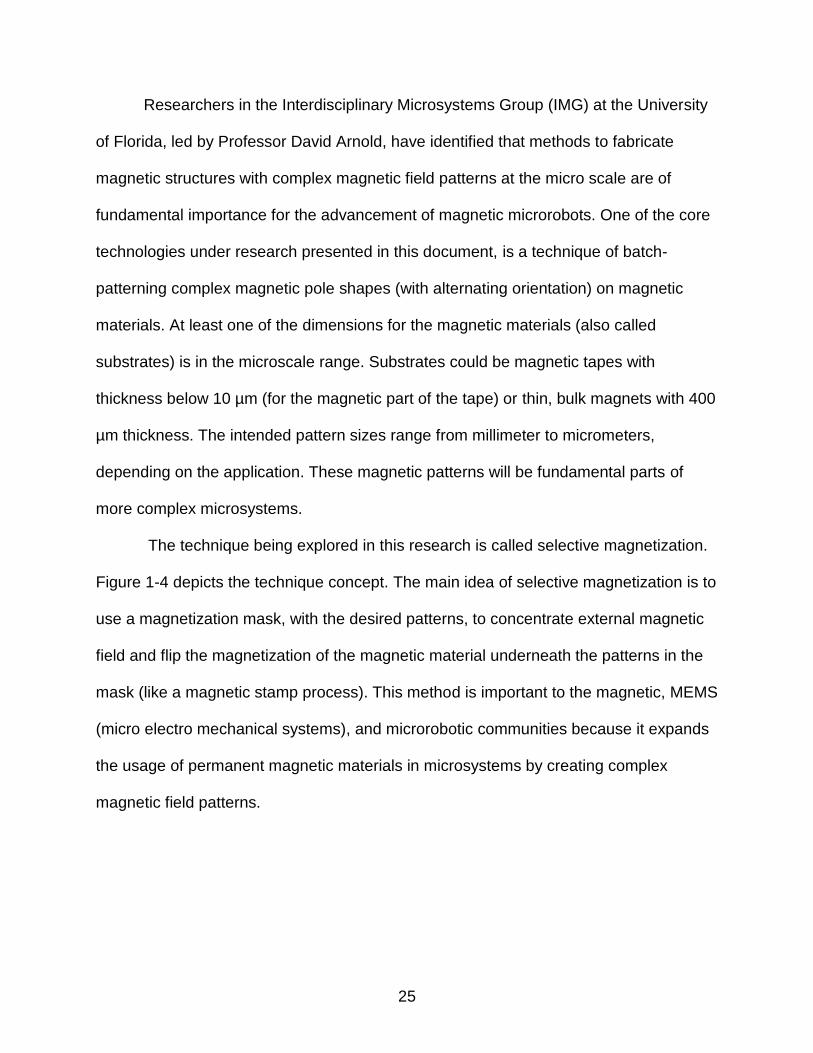
Researchers in the Interdisciplinary Microsystems Group (IMG) at the University

of Florida, led by Professor David Arnold, have identified that methods to fabricate

magnetic structures with complex magnetic field patterns at the micro scale are of

fundamental importance for the advancement of magnetic microrobots. One of the core

technologies under research presented in this document, is a technique of batch-

patterning complex magnetic pole shapes (with alternating orientation) on magnetic

materials. At least one of the dimensions for the magnetic materials (also called

substrates) is in the microscale range. Substrates could be magnetic tapes with

thickness below 10 µm (for the magnetic part of the tape) or thin, bulk magnets with 400

µm thickness. The intended pattern sizes range from millimeter to micrometers,

depending on the application. These magnetic patterns will be fundamental parts of

more complex microsystems.

The technique being explored in this research is called selective magnetization.

Figure 1-4 depicts the technique concept. The main idea of selective magnetization is to

use a magnetization mask, with the desired patterns, to concentrate external magnetic

field and flip the magnetization of the magnetic material underneath the patterns in the

mask (like a magnetic stamp process). This method is important to the magnetic, MEMS

(micro electro mechanical systems), and microrobotic communities because it expands

the usage of permanent magnetic materials in microsystems by creating complex

magnetic field patterns.

26

Figure 1-4: Selective magnetization concept.

1.1.2 Research Objectives

The general objective of this dissertation is to study the creation of complex

magnetic field patterns at microscale, and the usage of such patterns in the fabrication

and functionality of microrobots. The modeling describing the magnetic behavior and

fabrication of the magnetic structures must fulfill the geometric necessities of

microsystem fabrication.

There are two specific objectives, grouping designated tasks governing the

research conducted in this dissertation:

First, to provide strategies and demonstrate processes for batch fabrication of

magnetic microrobots, using selective magnetization as a fundamental technology.

Designated tasks are: to demonstrate feasibility of patterning complex magnetic field

patterns, to model and validate the selective magnetization process, to propose and

execute fabrication techniques for multiple magnetic structures in a batch process,

propose a technique for particle capturing at the boundary of magnetic poles, and

generate diamagnetically levitating micro-robot bases.

Bext Bext

Magnetic layer (initial state)

NO Magnetized

MagnetizedUP

Magnetized DOWN

Magnetizationmask

Strong magnetization

Reverse magnetization

Selectively magnetized pattern

Bext

Bext

27

Second, to suggest mechanisms to enhance functionality of microrobots, in terms

of interaction with the objects to be manipulated. These mechanisms could be

implemented over existing microrobotic platforms. Designated tasks are: to prove

feasibility of a magnetically detachable end effector, to stablish a batch fabrication

procedure of end effectors for microrobotics, and to propose alternatives for

microfabrication of electropermanent magnets.

1.1.3 Research Methodology

A diagram in Figure 1-5 is presented as a general methodology for this research.

The proposed path to elaborate a simulated model is to start from understanding the

theory behind some specific natural phenomena or physical behavior. Next, elaborate a

theoretical model that describes a simple configuration of this phenomena. Then, use

this theoretical model to start the designing process, i.e. selection of components or

identifying general constraints in the problem. After, it is possible to elaborate a

simulation model that combines the theoretical model and de designed variables. The

objective of a simulation tool is to improve the design, therefore, better design

constraints and an iteration process will lead to a more accurate simulation. It is

important to have in mind that simulation is not the ultimate goal. With the design and

the simulation results, then it is possible to fabricate a prototype. Testing or measuring

this prototype will generate important information to validate or feedback the simulation

model. This work believes that multiple iterations on this loop will generate more

accurate results each time and will reduce time in future designs.

28

Figure 1-5: Modeling methodology concept diagram.

1.2 Dissertation Overview

Chapter 1 of the dissertation (Introduction) presents an overview of the potential

that microrobotics have in the global industry of robotics, as a justification for the

importance of the work presented in this document. It also explains the objectives

research contributions of the conducted research.

A detail analysis of the state of the art of microrobotics and magnetostatics at

small scale is presented in Chapter 2 (Background). Magnetostatics is fundamental to

develop validated models (analytical and numeric) that can predict the stray magnetic

fields of complex patterns

It is fundamental to elaborate the theoretical bases of magnetic forces at

microscales. Magnetic forces will be the physics governing the mobility mechanism for

the selected microrobots (diamagnetic levitated) and governing the fabrication principle

for the bottom-up approach (magnetic nanoparticle collection). Chapter 3 (Magnetic

29

forces at small scale) will explain the concepts and present and alternative solution to

the problem of measuring magnetic forces at small scales.

And overview of magnetic field patterning at microscale and a description of the

selective magnetization process is presented in Chapter 4 (Selective magnetization).

The chapter will also include description of a simulation model for the selective

magnetization process, fundamental to interpret the changes in variables involved in

this process and predict the stray magnetic fields of the fabricated complex patterns.

The micro-nanorobotics community (as a subset of the microsystems and

nanotechnology communities) considered two fabrication approaches: 1) the bottom-up

and 2) top-down [7]. Both approaches will be exemplified in this dissertation for

fabricating microrobots using magnetic field patterns. 1) A bottom-up approach,

centered in the idea of magnetically assemble nanoparticles onto the interface boundary

of magnetic patterns, then crosslinking the particles for later release them as magnetic

microrobots. This project will be presented in Chapter 5 (Microrobot fabrication: bottom-

up approach). 2) A top-down approach of microrobot fabrication will be addressed in

Chapter 6 (Microrobot fabrication: top-down approach) by demonstrating a batch

fabrication technique for diamagnetic levitated robots. The selective magnetization

technique will be used in this approach.

Once the microrobots are fabricated, it is time to give them additional

functionality. A first approach will be providing exchangeable/replaceable end effectors

with different “tools” to perform variety of tasks. The mechanism to attach every end

effector with the microrobot will be by using magnetic patterns. The fabrication

procedures will be presented in Chapter 7 (Adding functionality to microrobots: end

30

effectors). A second approach will be designing a complex magnetic pattern that can

turn on/off the external magnetic field. Such magnetic pattern is called electropermanent

magnet and will be explained and demonstrated in Chapter 8 (Adding functionality to

microrobots: electropermanent magnet).

Figure 1-6 presents a summary of the content of this document and how each

chapter is related with the specific objective for this research. This figure compress the

main spirit of this work. Remarks of the wok conducted in this document and a

summary of the accomplishment will be presented in Chapter 9 (conclusions).

Figure 1-6: Research and document description.

Magnetically

detachable

end effectors

Electro-

permanent

magnets

Background

Magnetostatics

Nanoparticle

assembly

Bottom-up

Diamagnetic

levitation

Top-down

Micro-magnetic

field patterns

MicrorobotsAdding

functionality

Chapters

Specific Objectives

Concepts

Selective

magnetization

Modeling

Multiphysics

Simulations

Validation

Magnetic

forces

31

CHAPTER 2 BACKGROUND*

This chapter is design for future students and researchers exploring the field of

microrobotics for the first time. The goal of this chapter is to lead the reader through the

brief history of microrobotics and point in the direction of the leaders of the field (in the

humble opinion of the writer). This literature review will cover the most important books

wrote about microrobotics and the review papers that summarize the work of many

research groups in the last 30 years across the world. This review is by any means

comprehensive, and many other authors should be included in the future, but it is a

starting point for the reader to discover the “big players” in this field that is still in its

infant stage.

This chapter also aims to illustrate some theoretical concepts of magnetostatics

and the modeling of magnetic materials at the microscale. Magnetostatic problems area

commonly simulated nowadays using finite element modeling These

modeling/simulation approaches are common topics in most of the modern magnetic

theory textbooks, but there are some important details that need to be considered when

modeling structures in the microscale domain, such as material magnetic

characterization (and corresponding demagnetization corrections). This chapter will

cover a simplified analytical model to evaluate the magnetic B field generated by

permanent magnets, as well as soft magnetic materials in the presence of external

magnetic fields. The model will be validated, demonstrating the accuracy and

* This section contains excerpts from reference [8] and [9]. Reprinted (adapted) with permission from C. Velez, I. Torres-Díaz, L. Maldonado-Camargo, C. Rinaldi, and D. P. Arnold, “Magnetic Assembly and Cross-Linking of Nanoparticles for Releasable Magnetic Microstructures / Supporting information,” ACS Nano, vol. 9, no. 10, pp. 10165–10172, 2015. Copyright 2015 American Chemical Society

32

possibilities of this research. A description of the importance of pole boundaries will be

also presented and described through simulations.

The magnetostatics section is divided in in seven sub-sections: 1) Classification

of the magnetic materials by interpretation of their material properties. 2) Introduction to

modeling magnetostatics. 3) Demagnetization correction for ferromagnetic materials, 4)

DC demagnetization will be mentioned. 5)Techniques used at University of Florida for

measuring stray magnetic fields and visualization of magnetic micropatterning will be

presented.6) Simulation methods and validations used as fundamental block for

modeling magneto static problems with finite element approach (single magnet). 7)

Simulation of magnetic pole boundaries. 8) Simulation of alternated magnetic pole

patterns in the form of a checkerboard.

2.1 Microrobotics

Since the first mention of small scale machines (called today microrobots) in

1959 by Richard Feynman [10], [11], numerous fields of applications for micro/milli

robotic systems have emerged such as minimal invasive medicine [12], bioengineering

[13], and microassembly [14]–[16]. Inspired by Feynman some visionaries such as A.M.

Flynn [17] and W. Trimmer [18], envisioning creating complex machines with sizes and

abilities of insects. Advances to achieve those goals were only possible by the progress

in the field of microsystems (MEMS), in microfabrication technologies [19] and specially

by using silicon as mechanical material [20].

Most of researchers working in the field of microrobotics, recognize their

inspiration in the founding works of R.S. Fearing [21], F. Arai and T. Fukuda [22], that in

the International conference on Intelligent robots and systems (ICIRS) on 1995, set the

fundamentals of micromanipulation and adhesive forces at microscale. Another

33

important founder in the 90’s was S. Fatikow who author or coauthor some of the first

books in the field.

A generation of researchers in the decade of 00’s brought exiting applications

and could be easily be named “parents” of the current research groups. During this

decade researchers in Europe leans towards biological applications and magnetic

actuation mechanisms (B. Nelson, M. Sitti, and O. Schmidt), meanwhile American

researchers lean towards enhance mobility in air and ground and industrial applications

(R. Pelrine, K. Pister, R. Wood, and D. Rus).

The decade of 10’s is still in its peak and many new groups have sprout, bringing

new challenges and facing interesting new problems. Each researcher in this generation

is working to develop new technologies and open new frontiers, therefore they could be

called the Progeny generation. Figure 2-1 depicts a genealogy tree with the most

important contributors in the field of microrobotics. This three is by any means extensive

(is a subjective representation based on visibility) and represents a starting point for

networking and research in the field. This tree will continue growing to become strong

and deliver impactful research.

Ronald S. FearingUC Berkeley

Biomimetic millisystems

Kristofer PisterUC BerkeleySmart dust

Metin SittiMax Planck Institute

Microrobotics

Robert WoodHarvard

Microrobotics

Kirstin PetersenCornell University

Bio insp. robot

Eric DillerUniversity of Toronto

Microrobotics

Bradley NelsonETH Zürich

Microrobotics

Lixin DongMichigan State University

Nanorobotics

Jake J. AbbottUniversity of Utah

Telerobotics

Fumihito AraiNagoya University

Micro/Nano Robotics

Toshio FukudaNagoya University

Intelligent Robotics

Sarah BergbreiterUniversity of Maryland

Microrobotics

Yves BellouardEPFL

Micromanufacturing

David CappelleriPurdue

Microrobotics

Igor PaprotnyUniversity of Illinois

Microrobotics

Sergej FatikowUniversität Oldenburg

Intelligent Robotics

Oliver SchmidtIFW DresdenMicromotors

Daniela RusMIT

Robotics

Sámuel SánchezMax Planck Institute

Nanorobotic biosensor

Richard FeynmanMicro-nano technology

William TrimmerBelle Mead Research

MEMS

1st generation(60’s and 80’s)

2nd generation(90’s)

3rd generation(00’s)

4th generation(10’s)

InspirationAlumni (PhD/postdoc)

Movie

Ron PelrineSRI internationalMicrofactories

Stephane RegnierUniversity of Paris VI

Microrobotics

Fantastic voyage1966

Big Hero 62014

Michaël GauthierFemto-ST

Micromanipulation

A.M. FlynnMIT

Mobile robots

34

Figure 2-1: Genealogy tree for microrobotics, containing the most cited researchers in the field.

Searching publications by “microrobotics” in google scholar (up to June 19th

2017) will result in 7.672 references, including patents and citations. A historical

representation of this references in Figure 2-2, will show an increasing trend

demonstrating the potential growth of the field. The field of microrobotics is in an infancy

stage and it can be proven by comparing number of references published in 2016 in

better stablished areas such as nanotechnology (74.100), MEMS (28.800), and

Robotics (~52.600). The field of nanorobotics have comparative numbers than

microrobotics, with a total of 5.790 references.

Figure 2-2: History of publications related with microrobotics (academic papers, references, citations). Source: Google Scholar.

2.1.1 Books About Microrobotics

If the reader is new to the field of microrobotics, two suggestions are offered: The

first (and most important) suggestion is to start familiarizing with the field by reading [23]

[24]. These references are two parts of the tutorial about robotics in the small (Part I:

557

0

100

200

300

400

500

600

196

5

197

0

197

5

198

0

198

5

199

0

199

5

200

0

200

5

201

0

201

5

202

0

Pu

blic

atio

ns

Year

Total references: 7.672

Source: Google ScholarSearch: Microrobotics

Include: Patents and citations

References in 2016:"MEMS" ≈ 28.800"Nanotechnology" ≈ 74.100"Robotics" ≈ 52.600

35

Microrobotics and Part II: Nanorobotics) published in IEEE Robotics & Automation

Magazine, prepared by Bradley Nelson’s research group. This is a very useful, clear

and introductory tutorial that summarizes the most important topics to be considered

when studying the field, such as scaling effects, forces, microfabrication,

micromanipulation, nature inspiration, power constraints, imaging and assembly.

The second suggestion is Chapter 18 in the Springer Handbook of robotics [25],

it is a guide into the micro and nano robotics world describing scaling, actuation

mechanisms (electrostatics, electromagnetics, piezoelectric), sensing techniques

(optical, electron and scanning probe microscopy), basic techniques in micro/nano

fabrication and microassembly. A classification of the microrobots based on their

functionality is presented and specific emphasis in bio-microrobotics is made. A general

description of nanorobotics with special emphasis on manipulation techniques is made.

After following these two introductory suggestions, the reader is ready to go in

depth into the field. Beneath, a list of books directly related to microrobotics (published

in English) and a brief comment on the content of each books. As mentioned before, the

microrobotics is a field that is in its infancy and probably many books will be written in

the future. Four groups of books will be presented: 1) Academic oriented books, 2)

books collecting papers about selected topic, and 3) conference proceeding books.

Academic oriented books

Researchers in Europe (specially France), have been leading efforts to structure

the field of microrobotics along books suitable for the academic environment. The

following three books could be perfectly used as text books in courses dedicated to

microrobotics. Each book presents a diverse perspective (mechanical, manipulation or

36

assembly). The constant in these books is the careful and meticulous explanation of

every angle of the topic.

Microrobotics: Methods and applications [26] (one of the favorite books of the

author of this dissertation), is a very complete book from the mechanical engineering

perspective of microrobotics. It is constantly supported by mathematical analysis and is

divided in three parts: Part I - Prerequisites. It explains the fundamental concepts of

linear elasticity and kinetics. Part II - Core technology. It makes descriptions of the

applied physics (scaling effect, adhesion forces, material structure and properties), the

flexures, actuators and sensors. Part III - Implementation, applications and prospects. It

describes state of the art microfabrication techniques and applications (and

technologies) that are driving the microrobotic field to the future.

Microrobotics for Micromanipulation [27] is a pedagogical book that covers the

principles of micromanipulation, from the perspective of the physics of the microworld

and the strategies of micro handling. It also includes the fundamentals of the actuation

mechanisms for the microrobotics (piezoelectric, electrostatic, thermal and magnetic)

and the overall architecture of a micromanipulation system. Class exercises and

projects on different topics, are an important inclusion of this book.

Even though, Robotic microassembly [28] is a compilation of documents from

different authors, it is carefully edited to present microassembly in the form of a

coherent book. It starts from modeling of microworld by describing the impact of

vacuum, liquids and roughness in the overall force analysis at microscale. A second

section dedicated to handling strategies at small scales, describes micro handling, self-

assembly and micromanipulation (in dry and wet environments). And a third section

37

called robotic and microassembly, is dedicated to industrial MEMS structures. It

evaluates strategies for 3D microassembly, high-yield automated procedures and micro

solder applications.

Micro-nanorobotic manipulation systems and their applications [7] offers a clear

explanation about the boundaries between the micro and nano world and describes

fabrication techniques using the top-down and bottom-up approaches. It describes the

physics at small scale by always pointing differences in both worlds. It dedicates a

section to the technologies and materials that enable research in both worlds and

explains in detail manipulation under optical and electron microscope. It evaluates the

complexity of manipulation and motility of three systems at small scale: bacteria flagella,

cells, and carbon nanotubes.

Intracorporeal Robotics [29] uses a simple classification to present this topic: the

scale size. It starts by describing principles, scientific issues and applications for

intracorporal millirobots, followed by paradigms, methods and devices used in

microrobotics. It has a special chapter dedicate by devices manipulating objects

bridging the micro and nano world (such as cells) and finalizes by defining the scientific

challenges for biomedical nanorobotics.

A special mention should be made to Microsystem Technology and Microrobotics

[30], to be the first book (to our acknowledge) dedicated to microrobotics. Its

introduction presented a worldwide analysis of the present and future of microsystems

(called microsystems technology –MST- in the book) and, even though, many of the

techniques available at the 90’s had evolved, it is still a reference point for studying

38

microrobotics. The book described the actuation principles and sensing mechanisms,

containing numerous examples.

Selected topics

Selected topics in micro/nano-robotics for biomedical applications [31], is an

effort to document research results in the biomedical field using micro/nano robotics.

The introduction of this book presents a clear description of the challenges presented to

the field of microrobotics in the future. In a systemic approach, four examples were

presented: biomedical image analysis, a programing a capsule robot to navigate in the

gastro-intestinal tract, optical tweezers for cell manipulation and catheter surgery

assisted by robots. In a device approach, the book presented alternatives to solve the

power problem in microrobots (towards autonomous systems) by the integration of fuel

cells and energy harvesting mechanism. The inclusion of a piezoelectric sensor was

also commented. Two examples were presented of applications using nanorobot, a

cooperative scheme for drug delivery and cancer target therapy.

Micro- and Nanomanipulation Tools [32], specially focus on manipulation of

biological elements such as cells (mechanic, magnetic, and optic manipulation),

bacteria, DNA, and organic molecules. It presents examples of manipulation for plant

pathology and untethered tools for surgery. It also presents non-biological examples of

manipulation techniques in optical induced electro-kinetics, nanomaterial manipulation,

scanning probe microscopes, atomic force microscopy, Industrial tools for

micromanipulation, scanning electron microscope, and magnetic helical structures.

Automated Nanohandling by Microrobots [33] is based on the assumption that

the primordial function of microrobots is the manipulation of object at nanoscale. It

evaluates diverse topics such as the trends, automation and problems of nanohandling,

39

the problem of controlling microrobots, tracking and imaging objects inside scanning

electron microscopes, characterization and handling of cells and nanotubes and

nanomaterials’ testing and modification.

Not all chapters in Advanced Mechatronics and MEMS Devices [34] are

dedicated to microrobotics, but it contains certain topics of interest to the microrobotics

community such as: microscale sensors (force-torque and elasticity), piezoelectric end-

effectors, miniaturization of micromanipulation tools, digital microrobotics, micro gripping

and bioinspired (biomimetic) microrobots.

Conference proceedings

Microrobotics : Components and Applications [35], is a proceedings book for one

of the first official conferences in the field of microrobotics. It is important because the

design and control methodology for microrobots was not well stablished. Important

contributors such as S. Fatikow, T. Fukuda, and F. Arai presented some of their first

work at this conference.

Small-Scale Robotics [36], is the proceeding of the first international workshop on

microrobotics at the International Conference on Robotics and Automation (ICRA). An

introduction on small scale presented examples of robots bridging the gap between

millimeter a micrometer fabrication. The main topic of this workshop was the mobility of

the microrobots and magnetically actuated was the predominate mechanism described

by the presenters. Six device examples were presented by different groups.

Two additional book chapters dedicated to microrobotic applications are of

interest: An applications in medicine (locomotion of legged microrobot in gastrointestinal

tract) could be found in section V of [37] and the simultaneous control of multiple

microrobots [38].

40

2.1.2 Review Papers in Microrobotics

If the reader is new to the field, it will be very useful to know in which direction

start looking for information. After considering books in the topic, the next logical step is

to search for review papers. At least 18 review papers have been written about topics

related to microrobotics. A brief description of the most important review papers is

presented below, by grouping the papers in three groups: 1) Actuation principles, 2)

biological applications, and 3) problematics in the field.

1) A first group of papers is traying to describe research efforts in the field of

microrobotics by presenting the trends and technologies [15] and describing the

actuation principles [39]. Two main principles are mainly discussed: Swimming and

Flying.

For swimming microrobots, magnetic actuation is one of the most important

mechanisms of locomotion, as mentioned before. This statement is demonstrated by

[40]. A subset of microrobots with magnetic locomotion technique but using rotating

fields and helical shapes is presented by [41].

For flying, a very comprehensive review of aerial robots (drones) is presented in

[42]. Three specific classification of flying microdrones is presented: micro unmanned

air vehicles (µUAV), micro air vehicles (MAV), nano air vehicles (NAV) and pico air

vehicles (PAV). It is important to highlight, that names in this classification are highly

influenced by marketing strategies and do not represent real dimensions.

2) A second group of review papers is entirely dedicated to biological/biomedical

applications. The environment of microrobots dedicated to these applications is mainly

liquid and it has its own special characteristics. Evidently, the mobility of the microrobots

in these environments requires special attention [43]. And untethered mobile

41

alternatives are desired [13]. New bio-inspired swimming microrobots arise [44], as well

as hybrids combining microfabricated structures with living bacteria [45]. Despite these

advances, most of the microrobots in biological applications remain to be manipulated

using magnetic fields [46]. Two specific goals are in mind in microrobots for biomedical

applications: the minimal invasive medicine [12] and theranostics (the fusion of

diagnostics and therapy) [47], that leans towards the usage of nanorobots instead of

microrobots.

In a side note and going in the direction of nanorobots, it is important to highlight

a review paper about the usage of carbon nanotubes in the field of nanorobotics [48].

3) The third group of papers is dedicated to describe solutions for two of the most

pressing problems for microrobotics: power and functionality. The problem of power

sources at small scales (with special orientation to remote sensors) is presented in [49]

and electrochemistry is presented as one of the alternative for solution [50]. The

problem of functionality is partially addressed by researchers in the neighbor field of soft

robotics. There is a recent interest in soft robotics because of the versatility and low

power consumption of these robots [51] [52]. This interest transcends into the

microrobotics field [53] making soft robotics an enabling technology for future

applications.

2.2 Understanding Magnetostatics

2.2.1 Classification of Magnetic Materials

The minimum magnetic unit in nature is defined as the magnetic dipole (can be

interpreted as a pair of charges or and equivalent small current loop). Not all elements

in nature respond the same way to an external magnetic field because each element

has an associated dipole magnetic moment ( m

in units of A·m2). This is the

42

fundamental unit to evaluate magnetic properties in materials. In the analysis of

elements more complex than dipoles, it is possible to consider the magnetization M

as

the measurement of the net magnetic dipole moments per unit of volume ( V ) as in

[54]:

V

m

VM i i

0

lim

2-1

For most of the applications involving homogeneous and isotropic materials (it

will be clear later that those materials are called diamagnetic and paramagnetic), their

magnetization will have a linear behavior in the presence of and external magnetic field

H

. This relationship is expressed as HM m

, were m is defined as the material

magnetic susceptibility. H

and M

are expressed in units of A/m.

It is possible to make a rough classification of every element (or materials) based

on their susceptibility ( m ). If 0m then the material is considered diamagnetic,

meaning that their internal magnetic dipoles will orient in antiparallel direction of any

external magnetic field. If 0m the material is considered paramagnetic, meaning that

their internal dipoles will align in parallel direction with the external magnetic field.

Another important property for materials is the relative permeability rµ defined as

m1 (some authors instead use µ , the material permeability as rµµµ 0). This

property is mainly used to characterize materials with non-linear behavior in presence of

external magnetic field. Those non-linear materials that have a net magnetic moment at

the atomic level and a strong coupling between neighboring moments are called

ferromagnetic. If the coupled neighboring moments are equal but aligned antiparallel to

43

each other (no net magnetic moment, therefore magnetization is zero), the material is

considered antiferromagnetic. Figure 2-3 shows the periodic table of elements with this

magnetic classification. It is important to notice that at room temperature (273 K) there

are only four ferromagnetic elements (iron, cobalt, nickel and gadolinium) and one

antiferromagnetic (Chromium).

Figure 2-3: Periodic table of elements illustrating their magnetic behavior at 273K. Adapted from © DoITPoMS, University of Cambridge, https://doitpoms.admin.cam.ac.uk/tlplib/ferromagnetic/printall.php.

Ferromagnetic materials are of special interest for this document. Their

magnetization curve( M

vs H

) sometimes present two values at each H

and its

interpretation depends on its prior state of magnetization. This behavior is called

hysteresis. The magnetization hysteresis curve will highlight two important properties:

remanence and intrinsic coercivity. The first property is evaluated without the presence

Po At Rn84 85 86

Ra88

Ac89

Gd64

Fe26

Co27

Ni28

FerromagneticParamagnetic

Antiferromagnetic

Diamagnetic

Cr24

Magnetism at temperature = 273K

H1

He2

Unknown

https://doitpoms.admin.cam.ac.uk/tlplib/ferromagnetic/printall.php

44

of external magnetic field ( H

=0) where the ferromagnetic material will present a

remanent magnetization ( rM ) that is called remanence. The sign of the remanence can

be either positive or negative depending on the previous magnetization direction, but

the positive and negative remanences generally have equal magnitude. The second

property is evaluated when the applied external magnetic field is in opposite direction of

the material’s magnetization. The internal magnetization of the material will change

direction if the external field is high enough ( M

will switch from positive to negative or

vice versa). The value of the external magnetic field to switch magnetization is called

intrinsic coercivity (ciH ).

Based on the intrinsic relative permeability, coercivity and remanence,

ferromagnetic materials can be classified in two groups: hard and soft ferromagnetic

materials. Hard ferromagnetic materials (also called permanent magnets) are

characterized for high intrinsic coercivity, high remanence and low relative permeability.

They retain the magnetic field and are very difficult to demagnetize (only by high

temperatures, large demagnetizing magnetic fields, mechanical stress, or chemical

damage). Soft ferromagnetic materials have lower intrinsic coercivity and remanence,

but they generally present very high permeability. This means that they will magnetize

very easily in the presence of an external magnetic field, achieving a maximum

magnetization value called saturation magnetization sM .

A special magnetic classification called superparamagnetic occurs for particles

with nanometer diameter. Because of their reduced volume, these particles can

spontaneously reverse their own magnetization due to thermal fluctuations even in the

absence of external magnetic field. Therefore, in a time-average sense,

45

superparamagnetic particles have zero intrinsic coercivity and zero remanence, but act

as ferromagnets in the presence of external magnetic fields. The external magnetic field

provides enough energy to overcome the thermal fluctuations in order to align the

magnetic moments with the field direction.

A comparison of magnetization curve of materials with different magnetic

classification is made by measuring their magnetic moments at different external fields

using vibrating sample magnetometer (VSM) (ADE Technologies EV9). The measured

moments are divided by the volume of each sample to obtain the magnetization. Figure

2-4 compares measurements made for following materials: diamagnetic (pyrolytic

graphite), paramagnetic (aluminum), hard-ferromagnetic (nickel coated NdFeB magnet,

grade N42 and reference B111 from K&J magnetics Inc.), and soft-ferromagnetic (AISI

1018 mild/low carbon steel). Superparamagnetic particles are also compared (iron

oxide nanoparticles embedded in a polystyrene matrix from Corpuscular Inc.), although

they were measured using superconducting quantum interference device (SQUID)

magnetometer (Quantum Design).

46

Figure 2-4: Measured magnetization curves of different types of magnetic materials. A) Full scale and B) Zoom-in into µ0M to compare diamagnetic, superparamagnetic and paramagnetic materials.

Because of the nature of the research reported in this document, it is of special

interest the magnetic properties of soft ferromagnetic materials. Using information of

commercial soft magnetic materials available in COMSOL library, Table 2-1 is created.

For uniformity, the table reports the relative permeability when the external field is 1 µT

(called µri). Tis field was chosen (~0 T) to guaranty data points in all materials. It also

reports the saturation magnetization (µ0*Ms in units of Tesla) when the external field is 3

T (~∞). It also presents the electrical conductivity of the materials (σ, in units of MS/m),

although this property will not be used during this document.

Table 2-1. Magnetic properties of some commercial soft ferromagnetic materials.

Material 1 µr [--] µ0*Ms [T] σ [MS/m]

Low carbon steel 1006 3882 2.1 8.4

Low carbon steel 1008 1221 2.1 8.4

Low carbon steel 1010 2119 2.1 8.4 Low carbon steel 1018 835 2.0 8.4

Metglas Nano Finemet 50 Hz 87031 1.2 0.8 Nickel Steel Molypermalloy (Alloy 79) 65709 0.8 1.7

Nickel Steel Permalloy Oriented 41882 1.1 1.7 Nickel Steel Mumetal 80% Ni 79518 0.7 1.7

Alloy Powder Core Ferrite 1229 0.4 1 µS/m Nickel Steel Supermalloy 445540 0.8 1.7

A B

-0.0015

-0.0010

-0.0005

0.0000

0.0005

0.0010

0.0015

-3.0 -2.0 -1.0 0.0 1.0 2.0 3.0

µo·M

[T]

µo·H field [T]

Soft ferromagnetic

Hard ferromagnetic

Superparamagnetic

Paramagnetic

Diamagnetic-3.0

-2.0

-1.0

0.0

1.0

2.0

3.0

-3.0 -2.0 -1.0 0.0 1.0 2.0 3.0

µo·M

[T]

µo·H field [T]

Soft ferromagnetic

Hard ferromagnetic

Superparamagnetic

Paramagnetic

Diamagnetic

47

Silicon Steel NGO Arnon 7 3333 1.5 2.1 1 µr measured at 1 µT / 2 µ0*Ms measured at 3 T

Figure 2-5 is a graphic representation of the magnetic properties of commercial

available soft ferromagnets (data obtained from COMSOL library). Each element is

allocated corresponding to its material properties, where the x axis represents the

saturation magnetization in units of Teslas, they y axis represents the relative

permeability, and the diameter of the marker represents the electrical conductivity.

Figure 2-5B represents a zoom- in view of the material properties for selected low-

carbon steels.

Figure 2-5: Material properties comparison for some soft ferromagnets in COMSOL library. A) Full list of materials and B) zoom in to low carbon steels.

2.2.2 Magnetic Model of Ferromagnetic Materials

Numerous applications related with magnetic phenomena require the usage of

hard ferromagnetic materials. Having a theoretical model that can predict the magnetic

field produced by a hard magnet with any geometry will be ideal. Although, because of

the nature of the physics in magnetism, the resulting equations (individual solutions of

the Maxwell’s equations) will be extremely complicated. The most common approach to

recreate the stray magnetic field of any shape is by using finite element models (FEM).

A B

48

A fundamental step, whenever using numerical methods is to validate the

simulations. To this goal, it is always recommended to solve a very simple problem (with

the most basic geometries) and to compare the analytical solution with the simulation

results. This step will give the researcher the confidence to explore further complicated

geometries, assuming accurate results. To the purpose of this dissertation, the

validation will be done by calculating the stray magnetic field produced by a sphere of

hard ferromagnetic material and compare the results with a COMSOL simulation.

Simulation and analytical model will be both compared with measurements of the

magnetic flux density to obtain a full validation of our models.

This problem requires the solution of Maxwell’s equations where there is no time

variation. This leads to cancel (neglect) the time-dependent terms in the equations. It

will also be of interest to consider a current-free problem where only the magnetic

component of the equations remains, narrowing the set of equations to a theory called

magnetostatics ( 0 H

and 0 B ). This theory also includes the constitutive

equation (from the Sommerfeld convention):

)(0 MHµB

2-2

where B

is the magnetic flux density in Tesla, H

is the magnetic field strength in A/m,

M

is the magnetization in A/m and AmTµ /104 7

0 is a constant representing the

permeability of free space. Further results will be derived based on theory from [54]–

[56].

The problems that will be solved ahead will be using the charge model as a

method to analyzing the magnetic field. Therefore, by using one of the propositions for

calculus, where the irrotational vector filed can be written as the gradient of a scalar-

49

valued function, another important term arises: the scalar potential m . This final term

will be useful to describe the magnetic field as:

mHH

0 2-3

By substituting Equation 2-2 and 2-3 into 0 B

(from Maxwell’s equations) the

magnetostatic Poisson equation can be obtained:

Mm

2 2-4

The Poisson equation is the fundamental part of the charge model and it is used

to find the magnetization field of a ferromagnetic material in any point of the space. The

problem with this differential equation is the enormous complexity of its solution for

complex geometries. As mentioned before, this is the main reason why it is necessary

to use finite element models (simulations) to predict magnetic fields of complicated

structures. A schematic of the sphere to be analyzed is presented in Figure 2-6. Figure

also depicts the selected coordinated system and conventions to calculate the magnetic

flux density in the point P.

Figure 2-6: Coordinate system for the calculation of the magnetic field in a point P near a spherical permanent magnet.

50

The assumptions are: the sphere of radius a, uniformly magnetized with

saturation magnetization sM (could also be interpreted as remanent magnetization) in

the direction z , the sphere is made of isotropic permanent magnet material and it is

suspended in free space. For a better solution of the problem it is necessary to

represent the Laplace equation (specific case of Poisson equation when 02 m ) in

spherical coordinates. This solution can be found in [54]. The solution of the magnetic

flux density can be calculated for two values of radius ( ar and ar ). Those two

values represent the field inside the sphere and the field outside the sphere respectively

in Equation 2-5.

arrr

aMµ

arzMµ

B

s

s

)sin()cos(23

1

3

2

3

3

0

0

2-5

An experimental setup is installed to measure the magnetic flux density of a

permanent magnet sphere and compare the results with preliminary COMSOL

simulations and the theoretical model presented before. A NdFeB sphere with 2”

diameter, grade N42 from K&J magnetics was measured using a gaussmeter (F.W.

Bell, series 9950) and a micro positioner. The material magnetization of the sphere is

estimated to be sM =926 kA/m, based on vendor specifications and by measuring the

maximum B field in the surface of the sphere, that should be sMµ0)3/2( (~776 mT).

Comparative results are presented in Figure 2-7 and show very good agreement. The

positioning error of the hall probe is calculated to be ~200 µm (probably the error in the

position of the sensor inside the probe).

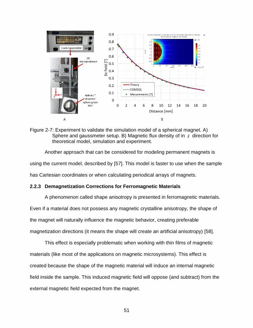
51

Figure 2-7: Experiment to validate the simulation model of a spherical magnet. A) Sphere and gaussmeter setup. B) Magnetic flux density of in z direction for theoretical model, simulation and experiment.

Another approach that can be considered for modeling permanent magnets is

using the current model, described by [57]. This model is faster to use when the sample

has Cartesian coordinates or when calculating periodical arrays of magnets.

2.2.3 Demagnetization Corrections for Ferromagnetic Materials

A phenomenon called shape anisotropy is presented in ferromagnetic materials.

Even if a material does not possess any magnetic crystalline anisotropy, the shape of

the magnet will naturally influence the magnetic behavior, creating preferable

magnetization directions (it means the shape will create an artificial anisotropy) [58].

This effect is especially problematic when working with thin films of magnetic

materials (like most of the applications on magnetic microsystems). This effect is

created because the shape of the magnetic material will induce an internal magnetic

field inside the sample. This induced magnetic field will oppose (and subtract) from the

external magnetic field expected from the magnet.

52

A way to understand this phenomenon is by representing the hard ferromagnet

using the charge model. It is easy to observe that north and south magnetic poles are

represented as a collection of positive and negative charges, respectively. Using this

convention, the stray magnetic field H

will create flux lines outside of the magnet

starting from positive charges and ending in negative ones. It is only logical that inside

the magnet the magnetic field will create the same lines from positive charges to

negative ones. The resulting H

lines inside the magnet are called demagnetization

field and are in opposite direction of the magnetization of the material.

It is very important to account for this demagnetization field (correcting the

measurement) whenever a material (with a shape different than a sphere) is being

characterized. Otherwise the resulting values will not represent the real properties of the

material and will lead to design or simulation errors. It is important to remember that one

of the goals is to use the correct measurement of magnetic properties as an input for

simulation models.

To have a correct demagnetization correction, the first step is measuring the

magnetization curve of the material using a magnetometer. The magnetization curves of

all the ferromagnetic materials described below were measured using a vibrating

sample magnetometer (VSM) (ADE technologies) with maximum applied fields of 2.26

T. This technique reveals the average distribution of the magnetization of the bulk

sample. To calculate the total internal magnetic field of a sample ( H

) including the

demagnetization, it is necessary to use the formula [59]:

53

MNHH appl

2-6

where applH

represents applied magnetic field by the VSM and M

is the magnetization

measured by the instrument. According to this notation, N is a symmetrical tensor [58]

[59] that contains the demagnetization factors: xxN ,

yyN and zzN . All other non-diagonal

factors are =0. These demagnetization factors will be related to the geometry of the

sample; every factor will be related with the corresponding coordinate axis (x y and z)

and 1 zzyyxx NNN . Calculating each demagnetization factor is not an easy task,

each sample geometry will have different set of equations for its calculation. This

dissertation focus on magnets with a prism geometry and their demagnetization factors

can be found in [60].

Consider a cuboidal magnet (rectangular prisms) as shown in Figure 2-8, with edge

dimensions in the x, y, and z directions of a2 , b2 and c2 . The magnet is subjected to a

magnetic field in the z direction. For thin samples with square area, i.e. ba , a term

acp / is created for simplification. According to [61] the calculation of zzN leads to :

54

p

121)+(p

3

2

3p

2

3p

)p2(12)+(p

3p

)p2(1

2)+(p

1arctan2

12)+(p

1-2)+(plnp1+2ln

p

2

1-2)+(p

1+2)+(pln

p

1-p=

2

3/232

2

2

2

2

2

2

p

p

N zz

2-7

Figure 2-8: Coordinate system representation used to calculate the demagnetization coefficients. Reprinted from A. Aharoni, “Demagnetizing factors for rectangular ferromagnetic prisms,” J. Appl. Phys., vol. 83, no. 6, p. 3432, 1998., with the permission of AIP Publishing [60].

Based on this geometry (square shape in xy plane), the other two

demagnetization factors (xxN and

yyN ) are equal and can be calculated by

2/)1( zzyyxx NNN (because all factors should sum 1). The use of these theoretical

factors has been compared with observations of the saturation process in prisms by

[62].

An example of the demagnetization correction process, for an isotropic

ferromagnetic material of Pt/Co alloy (platibalt after 700ºC annealing for 40min) is

presented in Figure 2-9. It is important to notice how the out and in plane

measurements before correction present the shape anisotropy (they look very different),

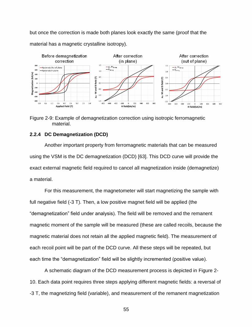
55

but once the correction is made both planes look exactly the same (proof that the

material has a magnetic crystalline isotropy).

Figure 2-9: Example of demagnetization correction using isotropic ferromagnetic material.

2.2.4 DC Demagnetization (DCD)

Another important property from ferromagnetic materials that can be measured

using the VSM is the DC demagnetization (DCD) [63]. This DCD curve will provide the

exact external magnetic field required to cancel all magnetization inside (demagnetize)

a material.

For this measurement, the magnetometer will start magnetizing the sample with

full negative field (-3 T). Then, a low positive magnet field will be applied (the

“demagnetization” field under analysis). The field will be removed and the remanent

magnetic moment of the sample will be measured (these are called recoils, because the

magnetic material does not retain all the applied magnetic field). The measurement of

each recoil point will be part of the DCD curve. All these steps will be repeated, but

each time the “demagnetization” field will be slightly incremented (positive value).

A schematic diagram of the DCD measurement process is depicted in Figure 2-

10. Each data point requires three steps applying different magnetic fields: a reversal of

-3 T, the magnetizing field (variable), and measurement of the remanent magnetization

56

at 0 T. In the example, 3 different data points were marked (for external fields equal to

0.2 T, 0.32 T and 0.4 T).

Figure 2-10: Schematic of the DC demagnetization measurement procedure.

Figure 2-11 illustrate an example of DCD curve for a hard ferromagnet (Pt/Co

platibalt) in plane and out of plane. As mentioned in the previews section, it is important

to correct the demagnetization of the material in any magnetization curve (including

DCD), to account for the geometry of the sample.

The DCD curve is important because it enables the determination of the

remanent coercivity ( rH ) which represents the required applied field at which the

measured remanent magnetization changes sign. One of the hypothesis of this work is

that the remanent coercivity is tightly related with the optimal external magnetic needed

to obtain a successful selective magnetization. Later in this document, the DCD curve

will be an input in the simulations to calculate the optimal external magnetic field to

-0.3

-0.2

-0.1

0.0

0.1

0.2

0.3

0.0 0.2 0.4 0.6 0.8 1.0

μ0 ·M

DC

D[T]

μ0·H field [T]

-0.3

-0.2

-0.1

0.0

0.1

0.2

0.3

-1.0 -0.5 0.0 0.5 1.0

μ0·M

fie

ld [

T]

μ0·H field [T]

Remanent coercivity: Hr=0.32 T

DCD curve

recoilsμ0·M

DCD

Magnetization curve

Demagnetization field = 0.4 T

Demagnetization field = 0.2 T

Demagnetization field = 0.32 TSteps in each

data point:

1) µ0·Hexternal = -3 T (Reversal)2) µ0·Hexternal = 0.32 T (demagnetization)3) µ0·Hexternal = 0 T (recoil)

57

generate the selectively magnetization and the resulting stray magnetic fields produced

by the successfully magnetized samples.

Figure 2-11: DCD in plane and out of plane of an example material. Before and after demagnetization correction.

2.2.5 Stray Magnetic Field Characterization

As mentioned by Patterson [64], the measurement of stray magnetic fields

produced by ferromagnetic materials is especially challenging at the microscale and

represents a technology gap that must be addressed by the MEMS community.

Professor David Arnold’s group at University of Florida have developed two

instrumentation systems with two different principles have been developed to enable the

visualization and quantification of the stray magnetic field at micro scale: The magneto

optical image (MOI) system and the scanning Hall probe microscope (SHPM).

Figure 2-12 illustrate the state of the art of the submillimeter magnetic field

measurement techniques (adapted from [64]), comparing each technique by its spatial

resolution in meters (x axis), the magnetic field sensitivity in Teslas (y axis) and the

frame scan time in seconds (color code). An ideal technique for magnetic fields in

58

microrobotics will have a spatial resolution between 10-7 to 10-3 and minimizing the field

sensitivity and the frame scan time.

Figure 2-12: State of the art of submillimeter magnetic field measurement techniques. Adapted from information on [64].

MOI is a technique that uses a magneto-optical indicator film as a lens for

reflective polarizing light microscope to image and quantify variations on the intensity in

a stray magnetic field. The magneto-optical indicator film leverages the Faraday effect

of a light wave crossing through special materials in the presence external magnetic

fields. The Faraday effect is a rotation of the plane of polarization, which is (to first

order) proportional to the field intensity and the film’s thickness, with the proportionality

constant known as the Verdet constant [65]. The fabricated MOI equipment, presents

field resolution between ±50 µT to ± 1 mT, field range between ±5 mT to ±230 mT,

spatial resolution of 4 µm, and average frame scan time in the order of few seconds.

Figure 2-13 illustrate the technique and presents an example image.

59

Figure 2-13: Magneto optical imaging (MOI) measurement technique. Reprinted from W. C. Patterson, N. Garraud, E. E. Shorman, and D. P. Arnold, “A magneto-optical microscope for quantitative measurement of magnetic microstructures,” Rev. Sci. Instrum., vol. 86, no. 9, p. 94704, 2015, with the permission of AIP Publishing [65].

On the other hand, the SHPM uses a Hall sensor/probe as a gaussmeter

mounted on 3D micropositioning stage for raster scanning magnetic fields in space and

reconstruct the image computationally. The main advantages of the technique are the

accuracy (electrical characterization), the high magnetic field range (>2 T) and high

spatial resolution. Unfortunately, because the rastering nature of the technique, the

drawback is the long scan time. The system built with this technique provides a range of

operation and resolution that can be adjusted by changing the currents in the hall probe.

The system also has a spatial resolution of 1.6 µm, raster scan resolution of 0.3 µm,

and average scan speed of 0.7 points per second. Figure 2-14 depicts the SHPM

technique and provides an example image [64].

Figure 2-14: Scanning hall probe measurement technique.

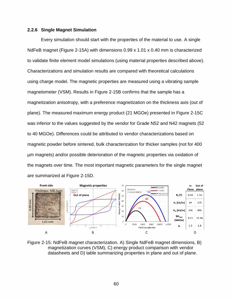
60

2.2.6 Single Magnet Simulation

Every simulation should start with the properties of the material to use. A single

NdFeB magnet (Figure 2-15A) with dimensions 0.99 x 1.01 x 0.40 mm is characterized

to validate finite element model simulations (using material properties described above).

Characterizations and simulation results are compared with theoretical calculations

using charge model. The magnetic properties are measured using a vibrating sample

magnetometer (VSM). Results in Figure 2-15B confirms that the sample has a

magnetization anisotropy, with a preference magnetization on the thickness axis (out of

plane). The measured maximum energy product (21 MGOe) presented in Figure 2-15C

was inferior to the values suggested by the vendor for Grade N52 and N42 magnets (52

to 40 MGOe). Differences could be attributed to vendor characterizations based on

magnetic powder before sintered, bulk characterization for thicker samples (not for 400

µm magnets) and/or possible deterioration of the magnetic properties via oxidation of

the magnets over time. The most important magnetic parameters for the single magnet

are summarized at Figure 2-15D.

Figure 2-15: NdFeB magnet characterization. A) Single NdFeB magnet dimensions, B) magnetization curves (VSM), C) energy product comparison with vendor datasheets and D) table summarizing properties in plane and out of plane.

61

Knowing the magnetic properties of the permanent magnet, it is possible to

predict the stray magnetic field produced in the surroundings. This task is just the

implementation of the theory available in textbooks using the charge model. Derivations

from Furlani 2001 [54] theory were implemented to obtain the expression for the z

component of the B field outside of a cuboidal magnet. A MATLAB code was created to

solve the book example for a magnet with dimensions: a=10 mm, b=20 mm and

c=10mm and sM =8.0x105 A/m. The Bz field was evaluate at z = 0.5 mm and z = 2 mm

and the results can be observed in Figure 2-16.

Figure 2-16: Analytical solution of the Bz field produced by a bar magnet and comparison with literature result. Reprinted from Permanent Magnet and Electromechanical Devices: Materials, Analysis, and Applications, First Edition, E. P. Furlani, Chapter 4 Permanent Magnet Applications, p. 217, Copyright 2001, with permission from Elsevier (Academic Press) [54].

62

Using a magneto optical image technique, developed by our group and

presented in [65], it was possible to evaluate and quantify the Bz field produced by this

single NdFeB magnet at different heights from above the surface (Figure 2-17).

Evaluated fields are compared with two models: 1) finite-element simulations (COMSOL

Multiphysics) using independent measured magnetization curves of the NdFeB material

and 2) an analytical solution assuming ideal magnetization [57] using the current model.

Figure 2-18 shows the comparison between measured, simulated, and theoretically

predicted Bz field, along the centerline of the magnet at increasing z heights. The tight

agreement of all three techniques confirms accuracy of the measurements.

Figure 2-17: Magneto optical images of a single NdFeB magnet at different heights.

63

Figure 2-18: Stray magnetic Bz field measurements using magneto optical images of an NdFeB square magnet and comparison with analytical solution and finite element modeling. Source: [64].

An additional reconstruction of the full vector B-field from a series of single axis

measurement images was made. First, Bz is measured in multiple planes above the

sample surface using the magneto optic measuring system. Then, because the vector

field is incompressible, the Bx and By components are reconstructed by calculating the

gradient of Bz with respect to x and y, and integrating the new dBz values in the z

direction. The continuous functions for Bx and By are converted into a discrete numerical

form to make them part of the measurement system’s post processing options and

finally are compared with the finite element model. The right side of Figure 2-19 depicts

the reconstructed Bx and By components of the field and the directly measured Bz.

Representations are calculated at a slice in the x-y plane 200 µm above the surface of

the magnet. Simulations show good agreement with the reconstruction of each field

component.

64

Figure 2-19: Bx, By and Bz reconstructions from single axis magneto optical images. Bz field measurements using magneto optical images of an NdFeB square magnet and comparison with finite element modeling (left side).

2.2.7 Magnetic Pole Boundary Simulation

After modeling a single pole magnet (previous section), the next logical step is to

model the boundary between two magnets: the first one magnetized up ( z direction)

and the second one in parallel but with opposite direction ( z

). Such case is presented,

for example, in perpendicular media recording; were specific areas of a thin magnetic

layer (e.g. films, substrates, tapes) are magnetized out of plane, in opposite direction of

the original magnetization of the layer. The interest of this configuration lies in the high

magnetic field and high magnetic gradient produced at this pole boundary. As it will be

explained later in Chapter 3, higher magnetic gradients correspond to high magnetic

forces.

65

To understand this behavior, a 2D magneto static finite-element simulation was

used to estimate the stray magnetic field at a magnetic pole boundary in a magnetic

substrate [66]. The simulation was made with COMSOL Multiphysics version 5.1, using

“Magnetic Fields, No Currents (mfnc) as the physics [67], [68]. A 2D cross section was

recreated with an air domain (17.5 µm height and 15 µm length) surrounding the

magnetic substrate (Hi8MP video cassette tape). The substrate domain was designed

with thickness and length of 1.75 µm / 15 µm and divided in two even ferromagnetic

segments with opposite magnetizations (as representation of two ideal magnetic poles

magnetized with opposite directions). As shown in Figure 2-20, the magnetization of the

substrate material was defined using demag-corrected magnetization curves measured

using VSM. Figure 2-21 presents the resulting B, M and H fields near the boundary.

Simulation of the field along the measurement line depicted in Figure 2-A was used to

generate Figure 2-21B and Figure 2-21C.

Figure 2-20: Magnetic properties of the substrate measured using VSM (second quadrant of hysteresis loop) and used as input for finite element model simulations. Dashed line represents the µ0M field and solid line represents the B field.

0.00

0.01

0.02

0.03

0.04

0.05

-75 -55 -35 -15

µ0 M

and B field [T]

H field [kA/m]

B

µ0∙M

Bµ0M

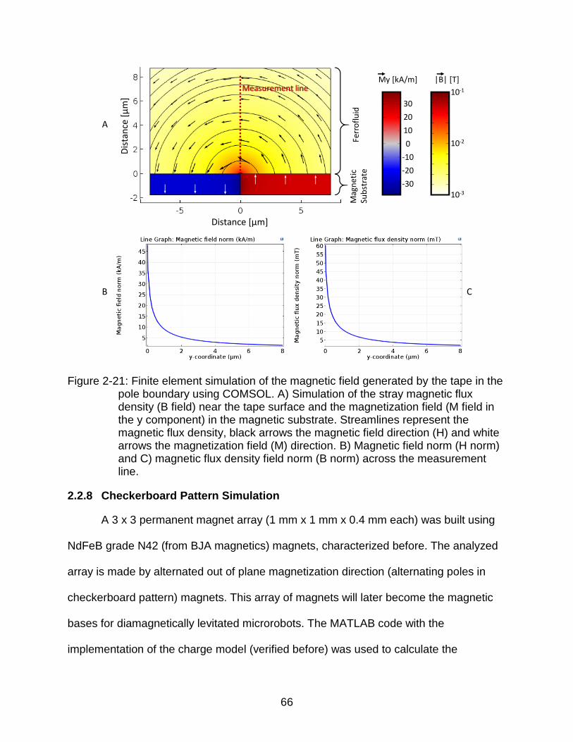
66

Figure 2-21: Finite element simulation of the magnetic field generated by the tape in the pole boundary using COMSOL. A) Simulation of the stray magnetic flux density (B field) near the tape surface and the magnetization field (M field in the y component) in the magnetic substrate. Streamlines represent the magnetic flux density, black arrows the magnetic field direction (H) and white arrows the magnetization field (M) direction. B) Magnetic field norm (H norm) and C) magnetic flux density field norm (B norm) across the measurement line.

2.2.8 Checkerboard Pattern Simulation

A 3 x 3 permanent magnet array (1 mm x 1 mm x 0.4 mm each) was built using

NdFeB grade N42 (from BJA magnetics) magnets, characterized before. The analyzed

array is made by alternated out of plane magnetization direction (alternating poles in

checkerboard pattern) magnets. This array of magnets will later become the magnetic

bases for diamagnetically levitated microrobots. The MATLAB code with the

implementation of the charge model (verified before) was used to calculate the

Distance [µm]

Dis

tan

ce [

µm

]

Mag

net

ic

Sub

stra

teFe

rro

flu

id

My [kA/m]

30

20

10

0

-10

-20

-30

|B| [T]

10-1

10-2

10-3

Measurement line

A

CB

67

analytical solution of the stray magnetic field in the surroundings. The concept of

superposition of magnetic fields was necessary to generate a solution for the array. An

example solution is presented in Figure 2-22.

Figure 2-22: Analytical solution of the Bz produced by a checkerboard pattern of 1mm ×

1 mm × 0.4 mm magnets with sM = 1,051 kA/m and calculations at z = 100

µm from magnets surface.

Additionally, a 3D COMSOL simulation was made using measured magnetic

properties of the materials. The result yielded a solution in good agreement with the

theoretical (charge) model, as can be observed in Figure 2-23. The results are

calculated at 50 µm from the surface of the magnet array.

Figure 2-23: Comparison between COMSOL simulation (using magnetization curve) and analytical model (charge model using saturation magnetization) for the magnetic field of the checkerboard pattern with 1 mm x 1 mm x 0.4 mm magnets.

68

2.3 Summary

This chapter presented a background of microrobotics. The most important

researchers in the field were introduced, the main books written to the date of this

dissertation were discussed and a list of the review papers was suggested as

introductory material to explore this field. A demonstration about the infancy of the field

was made, by comparing number of publications in 2016 with related fields.

An introduction to magnetostatics was made, providing tools for solving problems

in this field and to design magnetic microsystems that uses magnetic materials. The

used methodology is based on the acknowledge of the theoretical model, the magnetic

properties of the materials involve (characterization), the construction of a simulation

model, the fabrication and testing of a device and a final validation of the proposed

models. This process is always iterative. Because of this methodology, an accurate

simulation model was created and validated with the theoretical models and

experiments.

69

CHAPTER 3 MAGNETIC FORCES AT SMALL SCALE*

This chapter aims to discuss the relevant forces at small scale, that ultimate will

govern the locomotion of microrobots and the interaction with surrounding objects and

environment. This chapter is divided in five sections. The first section is a description of

all the forces presented at small by dividing them by the type of interaction with the

environment. The second section is the theoretical analysis of the magnetic force. The

third section presents an analytical solution for the forces exerted by two permanent

magnets. Section forth is dedicated to diamagnetic levitation. Finally, section five will

describe a novel implementation of a direct magnetic force measurement technique,

proposed for this research.

3.1 Relevant Forces for Microrobotics

Even though the laws governing physical behavior at the microscale are the

same as the macroscopic world, the relative importance of various physical laws can

dramatically change at small scales. For microrobotics, the interest relays on the forces

acting on a structure and they depend on the surrounding environment. However, the

importance of the forces in microrobotics is not entirely related to dimensions (size

scale) but also by the context of application (environment and application). Four

scenarios will be described to present the forces for microrobotics: 1) Forces interacting

at long range, 2) Surface and contact forces, 3) Hydrodynamic forces, and 4) Actuation

forces.

* This section contains extracts from reference [69]. Special thanks to Nicolas Garraud for their contribution on this chapter.

70

Presenting a proper explanation and a mathematical derivation of each of the

possible forces at microscale is beyond the scope of this document. The intention is to

introduce the reader to each force, present some relevant references that discuss more

carefully each force and in some cases use the scaling theory proposed by Trimmer in

[18] to compare the magnitude of forces to understand their importance. The following

analysis is limited for scale sizes between 10 nm and 1 mm. For analysis of forces

around the nanometer scale it is recommended to follow the work of nanorobots

presented by [24] and the study of forces in scanning probe microscopy by [70]. Only

the magnetic forces will be discussed in detail in the next section, for the relevance of

this force for the research projects described in this document.

3.1.1 Forces Interacting at Long Ranges

In this document, the expression “long range” means forces that start interacting

at the surfaces of the object and disappear several size-scale of the object under

analysis (interactions far from the object are the interest). The three forces that interact

in the long range are the gravitational force, the electrical (electrostatic) force and the

magnetic force. It is common to find the electric and magnetic forces named

electrophoresis and magnetophoresis, respectively (per the etymology, phoresis -

φόρησις - in ancient Greek that means “the act of bearing”).

A descriptive comparison of these three forces is presented in [23] and

summarized in Figure 3-1, where the force over the weight (assuming Earth’s gravity) of

an element is plotted at different sizes. The thought experiment considers how to lift

(against gravity) a sphere of conductive material of radius r (this will be the main

variable for scaling) and density ρ = 6.72×103 kg/m3 (as a fictional example). One way is

by using electrostatic (capacitive) force produce by an infinite plate, made of the same

71

material of the sphere, and potential difference U = 100 V. Another way is by using

magnetic force with a cylindrical permanent magnet of radius 4r and height 8r. Both, the

sphere and the cylinder are permanent magnets with magnetization M = 1.1×106 A/m in

the same direction (aligned). The distance between the sphere and the actuation

mechanism is αr, with dimensionless value of 1 or 0.1 (to evaluate the importance of the

sphere’s proximity to the actuation mechanism).

The gravitational force is one of the most important forces in the macroworld, but

often becomes minimized in the microworld. It is observed in the figure that the

magnetic force quickly surpasses gravity when r is below 1 m. The electrostatic force

surpasses gravity below ~100 µm. The electrostatic force surpasses the magnetic force

when r is below ~1 µm. This is a very important result because it presents the magnetic

forces as the strongest forces in the most common scales of operation of the

microrobots (1 µm to 100 mm). This analysis motivates specific focus on magnetic

forces.

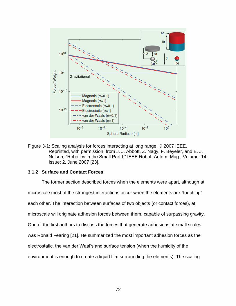
72

Figure 3-1: Scaling analysis for forces interacting at long range. © 2007 IEEE. Reprinted, with permission, from J. J. Abbott, Z. Nagy, F. Beyeler, and B. J. Nelson, “Robotics in the Small Part I,” IEEE Robot. Autom. Mag., Volume: 14, Issue: 2, June 2007 [23].

3.1.2 Surface and Contact Forces

The former section described forces when the elements were apart, although at

microscale most of the strongest interactions occur when the elements are “touching”

each other. The interaction between surfaces of two objects (or contact forces), at

microscale will originate adhesion forces between them, capable of surpassing gravity.

One of the first authors to discuss the forces that generate adhesions at small scales

was Ronald Fearing [21]. He summarized the most important adhesion forces as the

electrostatic, the van der Waal’s and surface tension (when the humidity of the

environment is enough to create a liquid film surrounding the elements). The scaling

Gravitational

73

analysis of the surface forces is presented in Figure 3-2A. Even though the figure is

extracted from [71], it is an adaptation of the original analysis made by Fearing.

Figure 3-2: Scaling analysis for surface forces. A) Force versus object radius. © 2006 IEEE. Reprinted, with permission, from Z. L. Z. Lu, P. C. Y. Chen, and W. L. W. Lin, “Force Sensing and Control in Micromanipulation,” IEEE Trans. Syst. Man Cybern. Part C Appl. Rev., vol. 36, no. 6, pp. 713–724, 2006 [71]. B) Force per unit area versus surface separation distance. Republished with permission of CRC Press, from Microrobotics : methods and applications, Y. Bellouard, first edition 2010; permission conveyed through Copyright Clearance Center, Inc [26].

Once again it is observed that the gravity diminishes with the reduction of the

scale. The surface tension is higher than the van der Waal’s forces, but scales at the

same rate (it is more difficult to separate wet surfaces than dry surfaces). Meanwhile the

electrostatic is weaker than the van der Waal’s below 1 mm but reduces faster. These

ratify the importance of the surfaces forces and how dominant they are in the

microscale. Of special interest in microscale are the van der Waal’s forces [72]. They

describe intermolecular forces and the importance increases when the objects have

dimensions below 10-7 m (as demonstrated in Figure 3-2). These forces became so

Forc

e [

N]

Forc

e p

er

unit a

rea [

µN

/m2]

10-14

10-12

10-10

10-8

10-6

10-4

10-2

10-4

10-2

100

102

10-6 10-5 10-4 10-3

Object radius [m] Surface separation distance [m]

10-9 10-8 10-7

A B

74

strong that manipulations objects at small scale became very challenging [73] (e.g.

when manipulate sub-micron size objects, releasing the object is very complicated).

A later analysis of the surface forces (with a more mechanical engineering

perspective) was made in Chapter 4 of Microrobotics Methods and Applications [26].

Additional experimental analysis of the physical phenomena made by Gauthier et al.

[74], separated these types of forces in two separated groups: 1) The surface forces

(non-contact), including the van de Waals, the electrostatic and capillary forces (as a

special form of the surface tension). 2) The contact forces, which includes the pull-off

force, as the force necessary to break the contact surface between two objects.

It is necessary to mention that from the perspective of the damage these surface

forces inflicted in objects, a different field of engineering emerged called microtribology

[75]. The force per unit of area is more relevant in this cases, as shown in Figure 3-2B.

In this example the analysis is made for two atomically-smooth SiO2 surfaces in close

proximity (surface sizes consider infinite compared with proximity). Instead of scaling

the size of the object it was scaled the distance between surfaces. This plot confirms

the importance of the capillary forces and how difficult result to overcome them. It also

illustrates how close the three forces became when reducing the scale (keeping the

charge constant). For this document purposes (and microrobotics in general) it

becomes more important to control and mitigate the effects generated by those forces.

3.1.3 Hydrodynamic Forces

Because many of the applications of microrobotics are in liquids, it is very

important to mention the forces experimented by objects in fluids at microscale. One of

the most complete descriptions of these types of forces is presented in [76]. It is evident

that the form and shape of the object affect the forces but for a dimensional analysis it is

75

possible to simplify the object as a sphere. In the field of microfluidics these spheres are

described as particles or even as “cells,” and the scaling analysis is made by changing

the particle diameter.

The main forces discussed in microfluidics are the buoyancy (capability to float

an object against the gravity), the Brownian (a random movement produced by random

collision of molecules of the fluid with the suspended particles), the Stokes’ drag (a

force that oppose the particle movement), and the lift (results in a velocity perpendicular

to the streamlines and is divided in two types: shear gradient-induced lift and boundary

layer lift).

Figure 3-3 presents a comparison of the hydrodynamic forces adapted from [76],

were a particle is moved by a magnetic force. As described by [77] the magnetic

actuation on particles is very common in these field, which is why it is included in the

figure. The selected velocity is 1 mm s−1 and channel width and depth of 100 μm. As

mentioned before, the gravitational force is once again present in the analysis, but in

fluidics, it is converted into the buoyancy force. It is important to mention that the

buoyancy and the magnetic force scales at the same rate, but magnetic force is

stronger. And is also important to show how the magnetic force became smaller than

the drag force for particles smaller than 1 µm. Finally, it is interesting how Brownian

forces are not problematic in the microscale but gain influence in the nanoscale.

76

Figure 3-3: Scaling analysis for hydrodynamic forces. Reproduced from M. Hejazian, W. Li, and N.-T. Nguyen, “Lab on a chip for continuous-flow magnetic cell separation,” Lab Chip, vol. 15, no. 4, pp. 959–970, 2015 ( http://dx.doi.org/10.1039/C4LC01422G) with permission of The Royal Society of Chemistry [76].

3.1.4 Actuation Forces

Another perspective to analyze the forces at microscale is regarding the

actuation mechanisms (actuators) for object positioning. It generally involves nanometer

positioning or displacement techniques. An analysis of these actuation forces was made

in Chapter 18 of the Springer Handbook of Robotics [25]. In this analysis, the three main

actuation forces are electrostatic, magnetic (electromagnetic) and piezoelectric. It also

mentioned that additional forces used in the field are thermomechanical, phase change,

shape memory, magnetostrictive, electrorheological, electrohydrodynamic and

http://dx.doi.org/10.1039/C4LC01422G

77

diamagnetism. Table 3-1 summarizes the actuation mechanisms that generate forces at

micro-nano scale and comments on the efficiency, the speed of actuation (on/off

commuting) and the power density required to actuate each mechanism. Each

characteristic is represented in the table with arrows denotating if is very high, high,

medium or low (e.g. Electromagnetic has high efficiency speed and power density

compared with others). The table shows electrostatic, electromagnetic and piezoelectric

are preferable actuation forces because their high efficiencies at high speeds.

Table 3-1. Comparison of actuation forces. Adapted from [25].

Method Efficiency Speed Power density

Electrostatic ↑↑↑ ↑ ↓ Electromagnetic ↑ ↑ ↑

Piezoelectric ↑↑↑ ↑ ↑

Thermomechanical ↑↑↑ ↔ ↔ Phase change ↑↑↑ ↔ ↑ Shape memory ↓ ↔ ↑↑↑ Magnetostrictive ↔ ↑ ↑↑↑

Electrorheological ↔ ↔ ↔ Electrohydrodynamic ↔ ↔ ↓

Diamagnetism ↑ ↑ ↑

↑↑↑ Very high ↑ High/Fast ↔ Medium ↓ Low

3.2 Theoretical Analysis of the Magnetic Forces

As mentioned before, the magnetic forces have great importance in the

microworld because their strength and the ability to use them for remote actuation. This

section will present magnetic forces using a differential analysis, due to the convenience

to use them on application were finite element model simulations are required. For

simplicity, no theoretical analysis of the stray magnetic field will be presented in this

section. This section was conceived thanks to the fundamental collaboration of Nicolas

Garraud.

78

3.2.1 General Expression for the Magnetic Force

Magnetism theory textbooks often start to analyze magnetic forces using the

magnetic dipole pair. Before 1988, there was a discrepancy among physicists about the

equation that models the magnetic force generated by this magnetic dipole pair. The

differences originated in the model for the dipole itself. The electric current loop model

leads to the force )( BmF

, where F

is the magnetic force, m

is the dipole magnetic

moment and B

is the magnetic flux density. If instead, the charge model is selected as

the magnetic model for the dipole then the resulting force will be BmF

)( . Timothy

Boyer [78] contributed to clarify the discrepancy in 1988, which is explained below.

Boyer highlights that differences between one or the other equation should be

considered depending on the specific application. But as a general analysis, he

proposed to expand the term )( Bm

using the vector identity to obtain:

mBmBBmBmBm

)()()()()( 3-1

Boyer explained that from Equation 3-1 the terms: mBmB

)()( will be negligible

in most of the applications, because a dipole should not have any space dependence

for m

(assumption that m

is independent of the spatial derivative because the dipole

definition). Later on in 1990 Vaidman [79] reinforce this concept and explained that in

term )( Bm

of Equation 3-1, a replacement could be made following Ampere’s law

as )( BJ

, with J as a current density. Therefore, if a specific problem does not

involve electric current, this term could be reduced as well. This leads us to consider

that for general purposes the dipole magnetic force where no external currents are

considered can be expressed in both ways BmBm

)()( .

79

In the doctoral dissertation [80], the author presents analytical models,

experiments and simulations to analyze both equations in the problem of calculating the

diamagnetic levitation force and the levitation height for a diamagnetic material

suspended over an array of magnets. In her conclusions, the most accurate model was

)( BmF

obtained from the current model.

No additional literature presenting substantial information related to the

comparison between these two models was found. Therefore, in this document the

magnetic force (in the magnetic particle assembly and in the diamagnetic levitation

problem) will be described using the current model in the form:

)( BmF

3-2

In a broader analysis of the force for elements more complex than dipoles, it is

possible to consider the magnetization M

as the measurement of the net magnetic

dipole moments per unit of volume ( V ) as in [54]:

V

m

VM i i

0

lim

3-3

In a differential analysis, the magnetization of a material with multiple magnetic

moments (m

) of the same magnitude and direction, in a differential of volume ( dV )

could be defined as dVMm

. Therefore, a differential of force ( Fd

) can be

interpreted from Equation 3-2 as )( BdVMFd

and because of the scalar nature of

dV we obtain:

80

dVBMFd )(

3-4

It is very important to make the following analysis, based on Equation 3-4: If we

imagine that the magnetization vector M

is in the same direction of B

, then the force

will be applied in the direction of the magnetic field gradient, B

.

Another important concept to consider is the magnetic torque [81]. A derivation of

the torque experienced by a magnetic material in an external magnetic field can be find

in Chapter 3.4 of [54]. Because the torque will not be used for any of the specific

applications covered in in this dissertation, the author refrains to present the full

derivation on this chapter. It is important to mention that the general formula for the

torque is obtained from the current model and it is always calculated in uniform external

magnetic fields (where 0 B

), to simplify the analysis. In its differential form, the

torque ( Td

in units of Nm) is presented as:

dVBMTd )(

3-5

Equation 3-4 and 3-5 are fundamental to understand the role of magnetism at

small scales (i.e. microrobotics). In an interpretation of them, the behavior of magnetic

objects at microscale can be summarized in the following two sentences (Figure 3-4): 1)

The object that experience an external magnetic field gradient, will feel an attraction and

will tend to be displaced towards the direction of the gradient (force). 2) The object in

the presence of a constant magnetic field will tend to rotate and align its magnetic

moment with the direction of the field (torque).

81

Figure 3-4: Interpretation of the magnetic force and magnetic torque at microscale.

3.2.2 Specific Cases for the Magnetic Force

Returning to the analysis of the magnetic force. Using Equation 3-4 as a general

expression for the force it is possible to obtain equivalent simplified equations for

several groups of problems, if the magnetization is interpreted based on its behavior

(non-linear, linear and constant) and its direction (aligned or not aligned with the

external field). These simplified equations are very useful in finite element model

simulations like COMSOL. Therefore, the following cases are presented:

Linear and not aligned

For most of the applications involving homogeneous and isotropic diamagnetic or

paramagnetic materials, their magnetization will have a linear behavior and can be

expressed as HM m

, were m is the material magnetic susceptibility and H

is the

field strength inside the material. This magnetic field is a vector and has its own

direction. If B

represents the magnetic flux density in the direction of the magnetic

source, then the force will be expressed as:

Magnetic Force

Magnetic Torque

dVBMFd )(

dVBMTd )(

Equation Action Direction

Displacement

Rotation

Gradient of the magnetic field

Align with the magnetic field

B

M

M

Interpretation

B

82

dVBHFd m )(

3-6

Linear and aligned

If the magnetization of the material is aligned with the applied magnetic field

(assumption in most of the cases), then the Sommerfeld convention can be used and

the field strength can be expressed in terms of the flux density using the permeability of

free space ATmµ /104 7

0

by the expression 0µ

BM m

and obtaining:

dVBBµ

Fd m )(0

3-7

It is important to remember that the dot product of two vectors

(2222

BBBBBBBBBBBB zyxzzyyxx

) is a scalar and the gradient operator (of

a scalar) result in a vector, as defined by:

zBBBz

yBBBy

xBBBx

BB zyxzyxzyxˆˆˆ)(

222222222

3-8

dVBµ

Fd m2

0

3-9

Constant and not aligned

In some applications when calculating the force over ferromagnetic materials, it is

common to search for expressions that consider the material when the magnetization

saturates at a constant value (referred as saturation magnetization sM ). In this case the

magnetization becomes MsnMM ˆ

, were Mn is the unitary vector describing the

direction of this scalar saturation magnetization. The force expression is then:

83

dVBnMFd Ms )ˆ(

3-10

Constant and aligned

Most of the multiphysics simulations over super paramagnetic nanoparticles

assume that the magnetization of the particles aligns instantaneously with the external

magnetic field (sometimes this is a very rough approximation). In these cases, it is

possible to describe the external magnetic flux density vector as the norm and direction

of the unitary vector: BnBB ˆ

and if the field and magnetization are aligned then

MB nn ˆˆ . Therefore, BMnBnMBM sBBs

ˆˆ because 1ˆˆ BB nn and the force

expression simplifies as:

dVBMFd s

3-11

Nonlinear and not aligned

Not all the ferromagnetic applications consider the saturation magnetization of

the material. Most of the times, the magnetization behavior of a material is presented by

a magnetization function (hysteresis curve in case of permanent magnets). When this

happens, the magnetization is represented as a vector function of the external magnetic

field )(HMM

. This case is the one that should be considered in most of the finite

element model simulations where is desired to include measured properties of

materials. The general force equation became:

84

dVBHMFd ))((

3-12

Nonlinear and aligned

Finally, when the magnetization vector function is aligned with the external field,

the dot product of them can be simplified as BHMnBnHMBM BB

)(ˆˆ)(

because MB nn ˆˆ and 1ˆˆ BB nn . The expression for the force in this case is:

dVBHMFd

)( 3-13

The following figure (Figure 3-5) summarizes the expressions of the magnetic

force based on the direction and behavior of the material magnetization in an external

magnetic field.

Figure 3-5: Magnetic force expressions based on the behavior and direction of the magnetization of the material.

3.3 Analytical Solution of the Force Between Two Magnets

In the previous section the force generated by an external magnetic field over a

magnetic object was explained, but in some applications, the magnetic field is produced

by another magnetic object. An example of this case is the force between two cuboidal

magnets. The solution is not trivial, it is related to the relative position of both magnets

and in most cases, it is better to use finite element model to compute that force.

dVBHm )(

dVBµ

m2

0

dVBnM Ms )ˆ(

dVBM s

dVBHM ))((

dVBHM

)(

Linear Constant Non linear

Not Aligned

Aligned

mFd

85

In 1984 Akoun and Yonnet [82] provided a 3D analytical solution for this problem

and experimental verification showing astonishing match. A later solution for the force

between two cylindrical magnets was presented by [83]. These generic calculations

were used to generate a “map” of the magnetic force in the space, by fixing the position

of one of the magnets and calculate the force in each point of the space meanwhile the

other magnet is displaced [84]. Based on these calculations, Robertson et al. [85], [86]

created a public framework for calculating forces between magnets and create a 2D plot

of these forces as a function of the position of one of the magnets. Using this

framework, a simplified case of one magnet separating from other in x axis is presented

in Figure 3-6.

Figure 3-6 Analytical solution for the force between two cuboidal magnets. Magnets displacement in x axis only.

Advancing the understanding of the magnetic forces, the following experiment

was made: If the moving magnet is orders of magnitude smaller (almost as a

“differential” magnetic volume) than the fixed one, then it is possible to raster it through

86

the entire area of the big magnet and obtain a 3D representation of the magnetic force.

Figure 3-7 illustrate this concept by calculating the magnetic force between a 3 mm × 3

mm × 0.4 mm NdFeB magnet (grade N42) and a 150 µm x 150 µm x 8 µm CoPt magnet

(not shown in the figure). The magnet separation is 296 µm. Because the superposition

of magnetic fields, this technique is useful to estimate the forces generated by

multipole-arrays of magnets. As it will be demonstrated later in section 3.5, these results

not only provide a better understanding of the array of magnets, but also serve as a

proof of concept for an alternative “force measurement” method. The forces between

two magnets can be used to characterize magnetic constructions at micro scales, such

as microrobots.

Figure 3-7: 3D representation of the analytical solution for the magnetic force between two cuboidal magnets when one magnet is one order of magnitude bigger that the other. Magnet separation is 296 µm.

3.4 Diamagnetic Levitation

Because of its curiosity, repulsive forces generate by magnetic fields over

diamagnetic materials are of high interest. According to Jiles [87], “Diamagnets are

solids with no permanent net magnetic moment per atom…Diamagnetism leads to very

weak magnetization which opposes the applied magnetic field”. A priori analysis of this

87

statement will lead to think that it is trivial to use these repulsive forces to suspend

(levitate) a magnet over a diamagnetic material or vice versa. Unfortunately, it is not.

The first set back is theoretical. For many researchers, levitating a magnet

appears to be a violation of the Earnshaw theorem [88]. In 1839 Earnshaw

demonstrated mathematically that a stable free suspension of a collection of particles

with the characteristics of a permanent magnet in vacuum is not possible. Earnshaw

proved that a configuration consisting of bodies that attract or repel one another with a

force proportional to the inverse square of the distance between them is always

unstable. The stability will come with the addition of other attractive or repelling forces

such as induced by currents. In a personal interpretation of this theorem, this will be true

if we are trying to find a stable state (suspension) in a configuration of only particles (or

permanent magnets) with the same characteristics. (In a satirical note: it is important to

recognize the limitations of the time when this paper was published and the fact that it is

trying to explain the constitution of the luminiferous ether).

An expanded theory of the possibilities and the conditions for free levitation was

given by Braunbeck [89], where it was stated that stable levitation is indeed possible

when a diamagnetic material is involved because the introduction of repulsive forces

that balance the attractive forces of the magnet. With this premise in mind, several

attempts to pursue diamagnetic levitation have been made. A complete history of

diamagnetic levitation can be found in [90], [91] where the concept has been used in

applications as diverse as sensors for structural monitoring in civil engineering [92],

energy harvesting [80], microfabricated rotors [93], biomedical applications [94],

88

acceleration sensors [95] and even to levitate frogs [96] (very iconic and controversial

research that won the IG Nobel Prize in 2000).

Although many of the elements in the periodic table are diamagnetic (copper,

gold, silver), not all are used for diamagnetic levitation. The two commonly used

materials for levitation are bismuth and pyrolytic graphite [97], because they are the

materials with the highest magnetic susceptibility at room temperature, with

10-16.6 -5m and 10-40.9 -5m respectively [98]. There are four configurations

to obtain diamagnetic levitation:

1) By levitating the diamagnetic material on top of an array of magnets with

alternated poles [95], [99], [100]. A variation of this technique is to use a single magnet

with selectively magnetized regions to obtain multiple poles [101].

2) By levitating a magnet using the diamagnetic material and additional magnets

to balance the forces (also called assisted levitation) [102], [103], [104].

3) An assisted levitation but replacing the balancing magnets by electric coils to

induce magnetic fields [105], [106].

4) To levitate the magnet over the diamagnetic material without balancing forces

[107], [108]. It is important to recognize the first to demonstrate the feasibility of levitate

a magnet over diamagnet without balancing forces was Pelrine in [109]. This technique

was used to fabricate levitated microrobots [110]. The microrobot is an array of cuboidal

magnets with alternated magnetic poles (checkerboard pattern), such as the one

presented in Figure 3-8.

89

Figure 3-8: Stray magnetic field of an array of magnets intended for diamagnetic levitation. Simulation obtained in COMSOL.

Using the charge model presented in section 2.2.6 (Figure 2-16) it is possible to

calculate the stray magnetic field produced by the array of magnets to be levitated as

microrobots. Additionally, following analysis on section 3.2.2 to calculate the magnetic

forces, the diamagnetic force can be understood by considering the magnetization of

the diamagnetic material always aligned with the applied magnetic field and with a linear

behavior for any applied field (negative susceptibility m ). Therefore, a differential

expression of such forces will be described by Equation 3-9: dVBµFd m

2

0 )/(

.

This analytical solution was experimentally confirmed by [80].

An analytical model is then created to predict the diamagnetic force produced by

the array of magnets, levitating on top of a diamagnetic surface. An example with

Mz

[MA/m]Bz

[T]

Black arrows represents B and white arrows represents M

90

magnets 3x3 NdFeB magnets (1 mm x 1 mm x 0.4 mm) with remanent magnetization

~1,051 kA/m over a pyrolithic graphite surface (4.8 mm x4.8 mm x 2.4 mm) with

susceptibility 51041 m was modeled. The parameters involved in the levitation will

be: the thickness and susceptibility of the diamagnetic material, the order of the

magnetic poles (+-+ or -+-), thickness, size and magnetic properties (remanence

magnetization) of the magnets. Figure 3-9 present a comparison of a magnetic array

reducing all parameters in half, the reference sample is the array called (- + -). This

model is a powerful tool to predict trends in the behavior of the magnetic force and will

be used later in this document.

Figure 3-9: Analytical solution to calculate the diamagnetic force. Sample is a 3 x 3 magnet array with alternated poles. Variation of all the parameters involve in the model.

0.01

0.1

1

10

100

1000

0 0.2 0.4 0.6 0.8 1

Dia

mn

etic

Fo

rce

[µN

]

Distance [mm]

- + -

+ - +

Half diam. thick.

Half susceptibility

Half thickness

Half magnetization

Half size

91

A more versatile model is desired, therefore finite element models (COMSOL)

were used to calculate the diamagnetic force, three steps are required. 1) Calculate the

quasistatic solution of the stray magnetic field (as in Figure 3-8). 2) Generate a map of

the magnetic force density in the space surrounding the magnets. This could be

obtained by calculating 2

0 )/( Bµm

on each point of the space, using the magnetic

susceptibility of the diamagnetic material. The force density units are N/m3. 3) Integrate

the force density values in the volume corresponding to the diamagnetic material. This

method simplifies the computational burden of the diamagnetic force, enabling the

calculation of diamagnetic forces in complex magnetic patterns.

Figure 3-10 illustrates the technique by presenting a cross section of the

magnetic force density generated by the magnets. To calculate the force generated by

the magnets suspended over block of pyrolithic graphite, it is only necessary to

integrate this force density function over the volume occupy by the pyrolytic graphite. As

hypothetical example, the diamagnetic force (if they were touching each other) between

and array of magnets and a block of pyrolytic graphite (5 mm x 5 mm x 2.5 mm), with

susceptibility 4104 m , will be 1.8 mN.

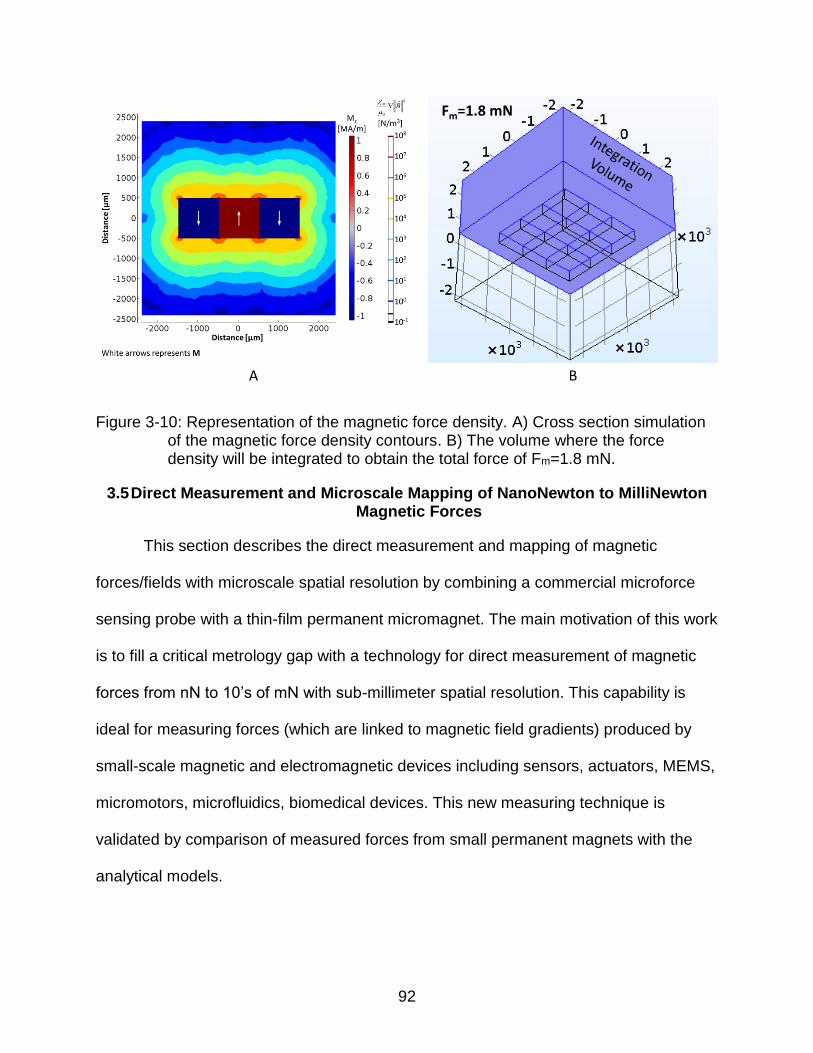
92

Figure 3-10: Representation of the magnetic force density. A) Cross section simulation of the magnetic force density contours. B) The volume where the force density will be integrated to obtain the total force of Fm=1.8 mN.

3.5 Direct Measurement and Microscale Mapping of NanoNewton to MilliNewton Magnetic Forces

This section describes the direct measurement and mapping of magnetic

forces/fields with microscale spatial resolution by combining a commercial microforce

sensing probe with a thin-film permanent micromagnet. The main motivation of this work

is to fill a critical metrology gap with a technology for direct measurement of magnetic

forces from nN to 10’s of mN with sub-millimeter spatial resolution. This capability is

ideal for measuring forces (which are linked to magnetic field gradients) produced by

small-scale magnetic and electromagnetic devices including sensors, actuators, MEMS,

micromotors, microfluidics, biomedical devices. This new measuring technique is

validated by comparison of measured forces from small permanent magnets with the

analytical models.

Fm=1.8 mN

A B

93

3.5.1 Measuring Magnetic Forces at Microscale

Ongoing technological advancements in microscale devices motivate the need

for magnetic force metrology at small spatial scales. Atomic force microscopy (AFM)

provides force sensing capability with sub-micron spatial resolution [111] and two

variants of scanning probe microscopy are capable of measuring forces produced by

magnetic fields: magnetic force microscopy (MFM) [112]–[121] and magnetic resonance

force microscopy (MRFM) [122]. While these techniques are well suited for measuring

forces at the micrometer and nanometer length scales, they are generally limited to

forces on the order of ~1 nN or smaller [123].

For measurements of larger forces in the nN to N range, microfabricated

microelectromechanical systems (MEMS) force-sensing approaches are well suited

[70], [124], [125], [126]. Contact-based microscale force measurements have been

made using vision-based (optical) [127], [128], [129] and capacitance sensing

mechanisms [130], [131]. However, non-contact magnetic force sensing at the

microscale has not been widely explored, but rather forces are inferred from magnetic

field measurement methods using Hall probe [132] or magneto-optical imaging (MOI)

[133] techniques. To infer forces from magnetic field measurements it is necessary to

calculate the magnetic field gradient (as described in Equation 3-4), which requires

multiple scans at different heights (at least two). Furthermore, noise and/or resolution

limitations in the measurement of B

can lead to significant errors in calculating the

gradient, and hence force, especially if the field gradients are small. Therefore, in

certain applications a direct force measurement is desired to decrease the

measurement time and potentially increase the accuracy.

94

This work reports the combination of a microforce capacitive sensing probe

(FemtoTools FT-S1000) [131] with a microfabricated permanent magnet as a sensing

probe yielding uniaxial magnetic force mapping capabilities at any point in space, with

microscale spatial resolution and nanometer positional accuracy. A similar construction

for sensing forces using MEMS devices and magnetic materials was previously

explored,[134], [135] but not intended as a force mapping tool. To validate the

construction of the proposed magnetic force sensing technique, an analytical model of

the force between two magnets was implemented and compared with experimental

measurements.

3.5.2 Experimental

As shown in Figure 3-11, an L10 CoPt micromagnet [136] (~150 µm x 150 µm x 8

µm) with out-of-plane magnetization serves as the “probe magnet” and is attached to a

microforce sensing probe (FemtoTools FT-S1000) [131]. The force probe is factory

calibrated to sense forces in the z-direction in a ±1000 µN range with 50 nN resolution

and cross-axis rejection factor of >30. The micromagnet is detached from the silicon

substrate on which it was formed and glued on the end tip of sensing probe using UV-

curable glue. The micromagnet is oriented such that attractive or repulsive forces acting

on the magnet are directed along the sensing direction of the force probe (along the

probe shank). The probe is then rastered at different vertical heights (from 25 µm to 200

µm) above a magnetic sample via a micromechanical testing station (FemtoTools FT-

MTA02) that facilitates a three-dimensional scanning range of 26 mm and minimum

step size of 1 nm in all three directions. Microforce sensing probes can be exchanged in

order to extend the force range from ±100 µN (5 nN resolution) up to 100 mN (5 µN

95

resolution). This means that the proposed technique can potentially measure magnetic

forces ranging from 5 nN to 100 mN.

Figure 3-11: Direct magnetic force measurement mechanism and overall experimental schematic. Force range 5 nN to 100 mN and displacement range of 26 mm in xyz.

The size, shape, magnetization direction, and material properties of the probe

micromagnet determine the magnitudes of the forces on the force sensor, as well as the

spatial resolution of the measurement. Figure 3-12A shows the micromagnet topology

as measured using an optical profilometer (Bruker Contour GT-I). Measurements of the

stray magnetic field at the surface of the micromagnet are made using a MOI method

(Figure 3-12B) [133]. The magnetization curves (Figure 3-12C) are measured using a

vibrating sample magnetometer (VSM) (ADE Technologies EV9) evidencing: Br=0.65 T,

Hc=405.8 kA/m, Hci=726 kA/m, BHmax=52 kJ/m3 and remanent magnetic moment

m=74 µemu.

Figure 3-12: Micromagnet characterization. A) Optical profilometer analysis. B) MOI measurements of the micromagnet Bz field and cross section values. Inset is

Raster directions

Force sensing probe

Micro MagnetM

M

Micromechanical testing station(FT-MTA02)

Microforce sensing probe(FT-S1000)

z

x

y

Force sensor with glued magnet

Force sensing probe

Micro magnet

-13.9 µm

-7.8 µm

Height

Dimensions: 148.6 µm x 146.0 µm x 8.0 µm

Optical profiler measurements

-1.0

-0.8

-0.6

-0.4

-0.2

0.0

0.2

0.4

0.6

0.8

1.0

-2.0 -1.5 -1.0 -0.5 0.0 0.5 1.0 1.5 2.0

Mag

net

izat

ion

: µ

0·M

(T)

Applied Field: µ0·H (T)

Hysteresis Out of plane

Hysteresis In plane

Cross section

-10

-5

0

5

10

Bz field [mT]

0 200 400 600 800 1000

X distance [µm]

0

200

400

600

800

1000

1200

Y d

ista

nce

[µ

m]

Micro magnet

0

12

Bz

Fiel

d [

mT]

6

A B C

96

a microscope image of the micromagnet. C) Magnetization curves for material out of plan and in-plane.

To create an “interesting” test sample for field mapping purposes, a 3 mm ×

3 mm x 0.4 mm N52 grade NdFeB magnet (BJA - Bob Johnson Associates, Inc.) was

used, exhibiting preferential out-of-plane magnetic properties, measured by VSM to be

Br=1.16 T, Hci=899 kA/m, BHmax=170 kJ/m3. The magnet sample was mechanically

polished to a surface roughness (Ra) of ~20 nm and then selectively magnetized using

the procedures described in Chapter 4 and by Velez, et al. [137] to imprint stripe-like

alternating negative and positive poles in the out-of-plane direction (perpendicular

magnetization). In brief, the magnet was initially magnetized upwards at 7 T and then

selectively reversed (downwards) using a 1-mm-thick low-carbon steel sheet (ASTM

A108) magnetizing mask subjected to a 1.5 T reversal field. The result of this process is

a patterned magnetic substrate where the imprinted poles have an estimated

magnetization of 0Mr=0.27 T. The stray magnetic field (Bz) generated by the

selectively magnetized test sample was characterized using magneto-optical image

(MOI) measurements at three different heights: 0 µm, 50 µm and 300 µm (Figure 3-13).

Figure 3-13: Magneto-optical image measurements of the magnetic field (Bz) produced by the 3 mm x 3 mm x 0.4 mm selectively magnetized test sample at different measurement heights. Comparative cross section plot (right).

2.5

2

1.5

1

0.5

00 0.5 1.511.5 0.51

X distance [mm]

Y d

ista

nce

[m

m]

0 µm from sample

Cross section

150 µm from sample

300 µm from sample

-200

-150

-100

-50

0

50

100

150

200

-1.5 -1 -0.5 0 0.5 1 1.5

Bz

fie

ld [

mT]

X distance [mm]

0 µm150 µm300 µm

Dimensions: 3 mm x 3 mm x 400 µm

0 50 150100150 50100B field [mT]

200200

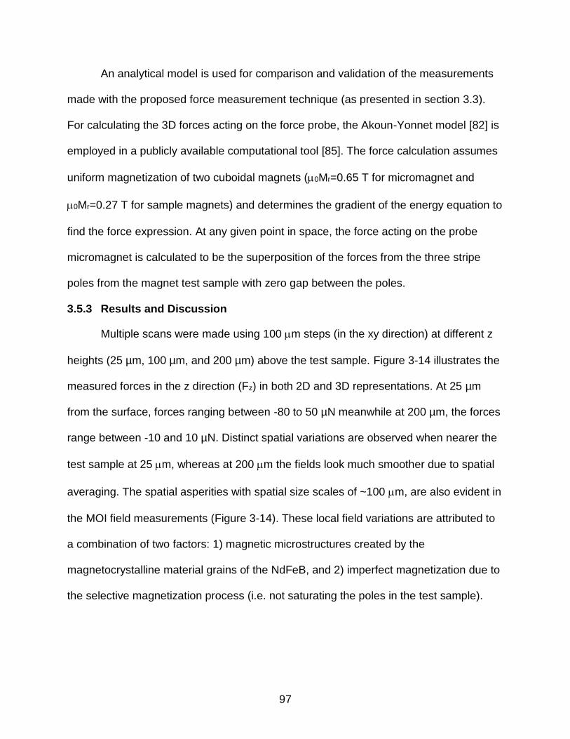
97

An analytical model is used for comparison and validation of the measurements

made with the proposed force measurement technique (as presented in section 3.3).

For calculating the 3D forces acting on the force probe, the Akoun-Yonnet model [82] is

employed in a publicly available computational tool [85]. The force calculation assumes

uniform magnetization of two cuboidal magnets (0Mr=0.65 T for micromagnet and

0Mr=0.27 T for sample magnets) and determines the gradient of the energy equation to

find the force expression. At any given point in space, the force acting on the probe

micromagnet is calculated to be the superposition of the forces from the three stripe

poles from the magnet test sample with zero gap between the poles.

3.5.3 Results and Discussion

Multiple scans were made using 100 m steps (in the xy direction) at different z

heights (25 µm, 100 µm, and 200 µm) above the test sample. Figure 3-14 illustrates the

measured forces in the z direction (Fz) in both 2D and 3D representations. At 25 µm

from the surface, forces ranging between -80 to 50 µN meanwhile at 200 µm, the forces

range between -10 and 10 µN. Distinct spatial variations are observed when nearer the

test sample at 25 m, whereas at 200 m the fields look much smoother due to spatial

averaging. The spatial asperities with spatial size scales of ~100 m, are also evident in

the MOI field measurements (Figure 3-14). These local field variations are attributed to

a combination of two factors: 1) magnetic microstructures created by the

magnetocrystalline material grains of the NdFeB, and 2) imperfect magnetization due to

the selective magnetization process (i.e. not saturating the poles in the test sample).

98

Figure 3-14: Force measurements at a different scan height above the test sample.

Figure 3-15 shows a comparison between the micromagnetic force

measurements (performed with 50 µm step size for maximum resolution) and an

analytical calculation [85]. The measurements show good general agreement with the

force model and prove the concept of direct magnetic force measurement.

25 µm from sample 100 µm from sample 200 µm from sampleM

agn

etic

Fo

rce

[µm

]

y coordinate [µm] x coordinate [µm]

x coordinate [µm]

y co

ord

inat

e [µ

m]

Mag

net

ic F

orc

e [µ

m]

Mag

net

ic F

orc

e [µ

m]

Mag

net

ic F

orc

e [µ

m]

99

Figure 3-15: Comparison of analytical model and force measurements at 100 µm tip-surface distance and 50 µm step size.

The limits of the proposed technique are calculated by hypothetically varying the

micromagnet size by changing the edge length from 1 µm to 1 mm, while keeping the

magnet thickness constant at 8 µm and assuming a constant out of plane magnetization

of the magnetic material (rM =426 kA/m). The force equation )( BmF

, reduced in

one dimension to dBz/dz=Fz/(V·Mr), where V is the volume of the micromagnet. Figure

3-16 shows the range of measurable field gradients (dBz/dz) versus magnet size. The

red region indicates the maximum and minimum possible force resolvable by the

microforce sensor platform using different probes (5 nN to 100 mN). The purple region

indicates the max and min force by the specific probe used in the results presented here

(50 nN to 1 mN). The field gradient range obtained from the fabricated magnet (150 µm

(a) (b)

30

20

10

0

-10

Magnetic Force [µN]

403020100

-10-20

Mag

ne

tic

Forc

e [

µN

]

Magnetic Force [µN]

30

20

10

0

-10

-20

-30

3D View

4020

0-20-40

Mag

ne

tic

Forc

e [

µN

]

An

alyt

ical

mo

de

l

-1 0 0.5 1

-1.5

Dis

tan

ce [

mm

]

Distance [mm]

1.5-0.5-1.5

-1

-0.5

0

0.5

1

1.5M

eas

ure

me

nt

-1 0 0.5 1

-1.5

Dis

tan

ce [

mm

]

1.5-0.5-1.5

-1

-0.5

0

0.5

1

1.5

Top View

100

edge length) is also highlighted from 0.7 T/m to 13,500 T/m). This plot highlights the

tradeoff between spatial resolution and field gradient resolution.

Figure 3-16: Magnetic field gradient limits detected by the proposed technique as a function of the micromagnet edge length. The equipment, the probe and the fabricated magnet detection ranges are highlighted.

3.6 Summary

This chapter described the relevant forces at small scale and highlighted the

importance of magnetic forces for microrobotic applications. The magnetic forces were

explained and a set of equations intended to be used in simulation models were

derived. The diamagnetic levitation was explained and calculated for a set of

simulations. A magnetic force sensing technique for force range of ±1000 µN with 50 nN

resolution and with a minimum step size of 50 µm has been demonstrated. The

actuation principle is by attaching a micromagnet (~150 µm x 150 µm x 8 µm) to a

commercial micro-force measuring probe (FemtoTools FT-S1000) and controlled by a

micromechanical testing station (FemtoTools FT-MTA02). Resulting magnetic forces

dB

z /d

z -

Ma

gne

tic

fie

ld g

rad

ien

t [T

/m]

Magnet edge length [µm]

10-2

10-1

100

101

102

103

104

105

106

107

108

109

1010

100 101 102 103

Calculations for fixed 8 µm thick magnet

Fab

rica

ted

m

agn

et

101

measured using this method were compared with the analytical solution of the forces

between two magnets (with one fixed and the other raster the surface). Measurements

and an analytical model present a good agreement.

102

CHAPTER 4 SELECTIVE MAGNETIZATION*

This chapter contextualize some of the techniques used nowadays by

researchers to solve the problem of creating magnetic field patterns at small scale. An

alternative technique called selective magnetization (briefly described in Chapter 1) will

be presented as a batch fabrication process for magnetic patterns. A simulation model

for the process will be presented and experimental results will confirm the existence of

an ideal reversal magnetic field for this process.

4.1 Patterning Magnetic Fields

The use of permanent magnets in MEMS (micro electro mechanical systems)

has been amply discussed by [138] and can track its origins back to the 1990’s with the

first implementations of micromotors [139]–[142]. Later on an extensive review on the

fabrication methods for integrating magnetic materials in MEMS was made by [143].

One important application of permanent magnets in microsystems is as part of

microscale power generators [144], and energy harvesting systems [145]. More recently

these power sources with permanent magnets as driving mechanism, have found

specific applications in bioengineering as energy generators for implantable medical

devices [146], powering biomedical sensors [147], and biomedical devices [148].

The use of permanent magnetic materials in MEMS was originally restricted to a

single magnetization direction, i.e. the entire magnet is “poled” in only one direction. In

contrast, at the macroscale, much more complex, three-dimensional magnetic field

arrangements are typically used to create desirable magnetic field patterns, such as

* This section contains excerpts from reference [8].

103

Halbach arrays [149]. These arrangements generally enable stronger magnetic fields

and/or field gradients, which enhance device-end effect performance. The ability to

create complex magnetic field patterns with sub-millimeter or even micrometer features

in MEMS can significantly broaden the utility of magnetic materials, and also enable

new microscale device architectures.

Previous attempts for creating complex magnetic structures (patterning) with sub-

millimeter features began with machining permanent magnets, individually magnetizing,

and assembling them [150]–[152]. Due to the high attractive forces between magnetic

poles the assembly is troublesome; furthermore, the lack of batch processing makes

large-scale manufacturing difficult. A more recent alternative is the inkjet-print of micro-

magnets [153], but this approach still requires additional permanent magnets to

guarantee a certain field orientation.

The solution presented in this work is to pattern (magnetically) permanent

magnet layers by “writing” magnetic poles with desired shape and orientation. As

mentioned by [144] and [154], this magnetic patterning is still one of the ongoing

challenges with this technology. For instance, Figure 4-1 shows three types of power

generation and all of them relay on the fabrication of complex magnetic shapes and

magnetized pole patterns that are difficult to integrate in a batch fabrication process.

Another example is the complex magnetic pattern for inertial rotation-based generators

presented in [147].

104

Figure 4-1: Three different types of permanent magnet power generation technology. Blue sections represent regions where pole patterns are required. © 2007 IEEE. Reprinted, with permission, from D. P. Arnold, “Review of microscale magnetic power generation,” IEEE Transactions on Magnetics, vol. 43, no. 11, pp. 3940–3951, 2007 [144].

The five mechanisms that are mainly used for magnetic micro-patterning are

described below. This literature review describes these mechanisms and presents the

most relevant work up to date.

First, poles can be created by generating spatially varying magnetic fields with

current-carrying conductors. This mechanism, published in 1998 by [155], proposed a

magnetization feature based on the magnetic field generated by passing current in a

conductor (Figure 4-2). The magnet was made out of plastiform flexible NdFeB and the

magnetized poles had minimum size of 42 mm (inner length for each one of the 6

segments in the ring). Magnetic flux densities were measured using a Hall effect

gaussmeter.

105

Figure 4-2: First magnetization mechanism by passing current. A) Schematic representations of single and double-sided axial field multipole magnetizing fixture. Reprinted from C. D. Riley, G. W. Jewell, and D. Howe, “The design and analysis of axial field multipole impulse magnetizing fixtures,” J. Appl. Phys., vol. 83, no. 1998, pp. 7112–7114, 1998, with the permission of AIP Publishing [155]. B) Magnetizing fixture used to multi-pole magnetize magnet plates of dimensions 50 X 50 X h mm3 with a pole pitch of 1 mm. Reprinted from J. Magn. Magn. Mater., vol. 270, Author(s), Töpfer, B. Pawlowski, H. Beer, K. Plötner, P. Hofmann, and J. Herrfurth, “Multi-pole magnetization of NdFeB magnets for magnetic micro-actuators and its characterization with a magnetic field mapping device”, pp. 124–129, Copyright 2004, with permission from Elsevier [156].

In [156], [157], the magnetization of 0.5 mm thick NdFeB magnets with 1 mm

pole pitch was reported. Poles were obtained by using pulse magnetization using wire

windings. Remanent induction of the patterns was measured using Hall probe scanning

and magnetic field reconstruction was made by software.

Using a configuration of wire windings and a soft ferromagnetic magnetizer, [158]

[159] present a planar micro-generator. A 8 mm diameter and 0.5 mm thickness disk

made of SmCo5 was magnetized with 15 pairs of poles. No direct measurement of the

magnetic fields generated by the magnet was documented. So far all groups working

with windings recognize that scalability below 1 mm is an issue.

A B

106

In the second mechanism, the composition of the magnetic material is modified

in order to locally change the coercivity of the material. If the material has predefined

areas with lower coercivities than others, then all the material can be strongly

magnetized in one direction and after, the field can be switched to a negative value

greater than the coercivity of sections with higher coercivity, but less than that of the

areas with lower coercivity.in order to create pole patterns. This mechanism was

presented by [160]. The entire permanent magnet was electrodeposited, but the regions

with different coercivity were generated by using patterned electrodes (with the desired

shape of the poles) that will alter the current conditions during the electrodeposition.

The current changes induce chemical modification of the magnet composition, therefore

the coercivity alterations. Poles of 450 µm were generated and the stray fields were

measured using a Hall probe.

The third mechanism to magnetize patterns on a permanent magnet is the

thermomagnetic patterning [161]. This method aims to reduce the coercivity of the

magnet by increasing the temperature locally, using laser irradiation through a mask. If

this heating process is done in the presence of external magnetic field (in the opposite

direction of the magnet’s magnetization), then the segments exposed to the laser will

change the orientation of their magnetization. This process is illustrated in Figure 4-3.

NdFeB films with thickness of 4 µm were magnetized with 50 µm pitch [162]. Scanning

Hall probe microscopy was used to measure the stray magnetic fields of the patterned

structures [162]. One drawback of this technology is the depth of magnetization

reversal, which was estimated to be 1.1 ± 0.2 µm. Later on, in [163] this depth was

107

increased to 1.3 µm. Thermomagnetic patterning has been mainly used in microfluidic

[163], particle capturing applications [164], [165], and cell capturing [166], [167].

Figure 4-3: Schematic diagrams of the thermomagnetic patterning process. Reprinted from F. Dumas-Bouchiat, L. F. Zanini, M. Kustov, N. M. Dempsey, R. Grechishkin, K. Hasselbach, J. C. Orlianges, C. Champeaux, A. Catherinot, and D. Givord, “Thermomagnetically patterned micromagnets,” Appl. Phys. Lett., vol. 96, no. 10, pp. 3–6, 2010., with the permission of AIP Publishing [161].

In order to increase the magnetization depth, a variation of the thermomagnetic

patterning was made by [168]. The external magnetic DC field was applied by an array

of permanent magnets and the heat process was conducted by laser beam scanning

(speed of 12m/s). A 4.5 µm thick NdFeB/Ta magnet over glass was magnetically

patterned with features between 70 µm and 100 µm. Magnetic flux density of the

patterns was measured using a Hall element.

The fourth mechanism relays on ion implantation or irradiation for patterning

magnetic films. This mechanism pertains the change in magnetization of selected areas

using ion irradiation or implantation results in a reduction of the magnetic anisotropy

108

[169]–[174]. The mechanism is explained in figure Figure 4-4. This mechanism, has a

bottom-up approach and it is more suitable for nanoscale magnetic patterning, but

because it’s relevance in the field it worth to be mentioned. Depth and size of the

magnetized patters are still in the order of hundreds of nanometers, and is a useful

technique for patterning thin magnetic films.

Figure 4-4: Sketch of the irradiation induced intermixing at the upper and lower Co/Pt interface. Reprinted from J. Magn. Magn. Mater., vol. 320, no. 3–4, J. Fassbender and J. McCord, Magnetic patterning by means of ion irradiation and implantation, pp. 579–596, Copyright 2008, with permission from Elsevier [169].

Lastly, in the fifth mechanism the magnetic fields can be shaped using soft-

magnetic magnetizing heads to selectively magnetize poles into magnetic layers. This

mechanism does not involve wire windings or altering physical properties of the magnet,

instead it uses ferromagnetic magnetized heads to imprint patterns on magnets. This

method was originally proposed by [175] [176] to pattern a SmCo magnet. Eight poles

were magnetized in a disk of 9.5 mm diameter and 0.5 mm thickness. A Hall sensor

measures the magnetic field. Dr Arnold’s group at University of Florida has continued

working on improving this method by varying the magnetization mask according to the

needs of the application. A laser and mechanical machined Hiperco50 mask (with 200

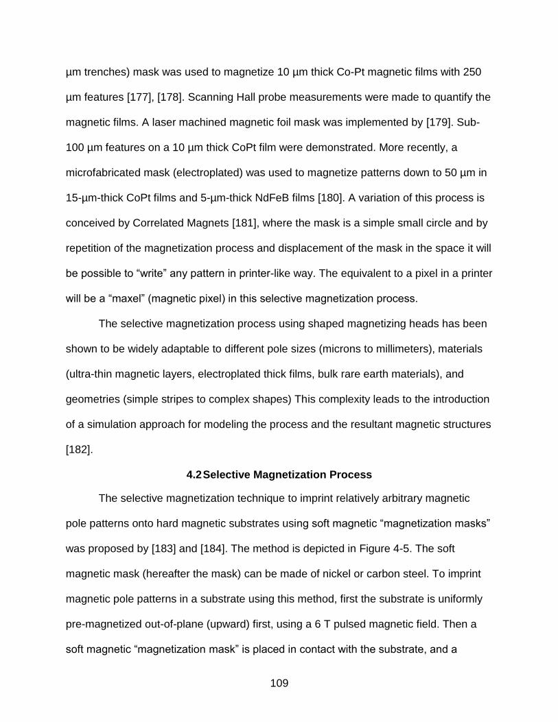
109

µm trenches) mask was used to magnetize 10 µm thick Co-Pt magnetic films with 250

µm features [177], [178]. Scanning Hall probe measurements were made to quantify the

magnetic films. A laser machined magnetic foil mask was implemented by [179]. Sub-

100 µm features on a 10 µm thick CoPt film were demonstrated. More recently, a

microfabricated mask (electroplated) was used to magnetize patterns down to 50 µm in

15-µm-thick CoPt films and 5-µm-thick NdFeB films [180]. A variation of this process is

conceived by Correlated Magnets [181], where the mask is a simple small circle and by

repetition of the magnetization process and displacement of the mask in the space it will

be possible to “write” any pattern in printer-like way. The equivalent to a pixel in a printer

will be a “maxel” (magnetic pixel) in this selective magnetization process.

The selective magnetization process using shaped magnetizing heads has been

shown to be widely adaptable to different pole sizes (microns to millimeters), materials

(ultra-thin magnetic layers, electroplated thick films, bulk rare earth materials), and

geometries (simple stripes to complex shapes) This complexity leads to the introduction

of a simulation approach for modeling the process and the resultant magnetic structures

[182].

4.2 Selective Magnetization Process

The selective magnetization technique to imprint relatively arbitrary magnetic

pole patterns onto hard magnetic substrates using soft magnetic “magnetization masks”

was proposed by [183] and [184]. The method is depicted in Figure 4-5. The soft

magnetic mask (hereafter the mask) can be made of nickel or carbon steel. To imprint

magnetic pole patterns in a substrate using this method, first the substrate is uniformly

pre-magnetized out-of-plane (upward) first, using a 6 T pulsed magnetic field. Then a

soft magnetic “magnetization mask” is placed in contact with the substrate, and a

110

reversal (downward) magnetic field pulse is applied (in the order of hundreds of mT).

The high permeability of the magnetization mask concentrates the magnetic flux in the

poles of the mask, thereby flipping the magnetization down in those areas. In the other

regions (between the poles underneath the air gaps of the mask), where the fields are

weaker, the magnetization remains in the original upward orientation.

Figure 4-5: Schematic of selective magnetization process. Magnetic tape is strongly magnetized. up (6 T). Then the magnetization mask is placed on top of the substrate, and a reverse magnetic field is applied. This reversal field selectively reverses the direction of the magnetization on the substrate, only in the areas underneath the mask.

The mask can be optimized by simulating feature sizes, separation between

structures, materials, and mask thickness. Every parameter variation involve in the

magnetization process can be simulated by using finite element method in COMSOL

Multiphysics.

4.2.1 COMSOL Simulation

The selective magnetization process is modeled using COMSOL Multiphysics

using a 2D simulation. The finite-element method is used to solve the magneto-quasi-

static Maxwell equations, following the methods reported in [182]. The experimentally

measured nonlinear magnetic properties of the substrate and mask materials

(magnetization curves) are used in the simulations.

111

Simulations are divided in two consecutive and dependent steps: first, the

application of the reversal magnetic field (Figure 4-6, top row), followed by second, the

stray field generated by the remanent magnetization in the substrate after selective

magnetization (Figure 4-6, bottom row). In the first step, the substrate is initially

considered uniformly magnetized up, and the simulation models the fields during the

peak of the downward selective reversal pulse. The result of this first step is then used

to calculate the conditions for second step. Following Samwel,, et al. [185], the

remanent magnetization at every point in the substrate is calculated using the DCD

curve. The DCD curve relates the peak field from step one to the resultant residual

magnetization used in step two. Step two of the simulation computes the stray fields for

the selectively magnetized substrate (with the magnetizing mask no longer present).

Figure 4-6: Selective magnetization process simulation (during magnetization – top row) and stray B field generated by the magnetic substrate after selective magnetization (after magnetization – bottom row). The M field inside the magnetic substrate and the mask.

Bext = 100 mT Bext = 400 mT Bext = 700 mT

Air

Magnetic substrate

0 0.5 1-0.5-1

-0.8-1

-0.6-0.4-0.2

00.20.40.60.8

1

Distance [mm]

After magnetization

During magnetization

-40

-20

0

20

40

M field [kA/m]

B field [mT]

-150

-50

0

50

150

100

-100

Air

Air Air

Magnetic substrate

Mask

Air

112

The sensitivity of the magnetization process with respect to the reversal B field

amplitude is evident in simulations shown in Figure 4-7, comparing reversal fields of 100

mT, 400 mT, and 700 mT. Figure 4-7 shows the profile of the predicted Bz stray fields at

50 µm above the surface of the substrate for the same three cases. For the 400 mT

case, the simulations indicate that it is possible to selectively reverse the substrate

through its entire thickness, as compared to the thermomagnetic patterning [161], [163],

which was limited to ~1 μm in depth. This case also yielding the strongest magnetic

stray field contrast. These simulations suggest there exists an ideal (optimal) reversal

magnetic field at which the substrate sections underneath the mask reverse without

affecting the magnetizations of the remaining substrate. Consequently, a parametric

series of simulations and experiments are conducted, varying the reversal B field from

50 to 1100 mT in order to determine the optimal field.

Figure 4-7: Simulations of the stray magnetic field comparison at 50 µm above the substrate for three reversal magnetic fields.

113

4.2.2 Magnetization Mask Machining and Model Validation

Figure 4-8 shows the magnetizing mask used in this section and the resulting

pole pattern of a selectively magnetized substrate. The mask has a simple stripe pattern

and is conventionally machined (using Sherline CNC) from AISI 1018 mild/low carbon

steel (relative permeability μr=102) with the feature size (line/space) of 1 mm and

feature depth of 0.6 mm. The magnetic substrate for selective magnetization is a flexible

iron oxide material with 0.57 mm thickness, remanence of Br=180 mT, and coercivity of

Hci=125 kA/m (μ0Hci=0.16 T).

Figure 4-8: Low aspect ratio magnetization mask. A) Schematic of the magnetization mask (gray) over magnetic substrate (orange). Red dashed lines represent the simulation line and the images taken using magneto optical images at 50 μm of the surface (shown late). B) Magnetization mask. C) Magnetized pattern on flexible iron oxide observed using magnetic viewer paper.

Magnetization fields from 100 mT to 1000 mT are applied using a pulse

magnetizer on independent samples. Magneto-optical images of each sample are taken

[65] using a 250 mT saturation magneto-optical indicator film at 50 μm above the

surface of the substrate. Figure 4-9A presents an example 3D representation of the field

pattern after magnetization, and Figure 4-9B presents the average measurement of the

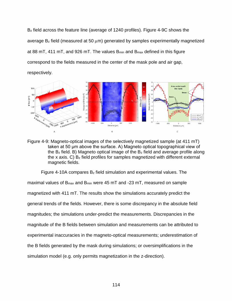
114

Bz field across the feature line (average of 1240 profiles). Figure 4-9C shows the

average Bz field (measured at 50 m) generated by samples experimentally magnetized

at 88 mT, 411 mT, and 926 mT. The values Bmin and Bmax defined in this figure

correspond to the fields measured in the center of the mask pole and air gap,

respectively.

Figure 4-9: Magneto-optical images of the selectively magnetized sample (at 411 mT) taken at 50 μm above the surface. A) Magneto optical topographical view of the Bz field. B) Magneto optical image of the Bz field and average profile along the x axis. C) Bz field profiles for samples magnetized with different external magnetic fields.

Figure 4-10A compares Bz field simulation and experimental values. The

maximal values of Bmax and Bmin were 45 mT and -23 mT, measured on sample

magnetized with 411 mT. The results show the simulations accurately predict the

general trends of the fields. However, there is some discrepancy in the absolute field

magnitudes; the simulations under-predict the measurements. Discrepancies in the

magnitude of the B fields between simulation and measurements can be attributed to

experimental inaccuracies in the magneto-optical measurements; underestimation of

the B fields generated by the mask during simulations; or oversimplifications in the

simulation model (e.g. only permits magnetization in the z-direction).

115

Figure 4-10: Measurement/simulations at 50 μm above the substrate for different reversal fields during magnetization. A) Bmax and Bmin B) B-field contrast.

As an overall figure of merit for the magnetization process, the magnetic contrast

is defined as [186]: C=(Bmax-Bmin)/(Bmax+Bmin). Figure 4-B shows a comparison between

the B field contrast from simulations and the experimental measurements. These results

confirm the existence of an optimal external magnetic field value at which the contrast is

maximized (~500 mT in this case). A contrast difference between simulations and

measurements is on the order of 29%.

4.2.3 Variations on the Selective Magnetization

To improve the selective magnetization procedure and make it viable for

magnetic substrates with high intrinsic coercivity and remanence (such as NdFeB)

some variations of the process were considered. It is necessary to remark that none of

the following configurations were used in future experiments, although they show

important learning lessons for future applications.

The intention of this set of experiments is to compare the selective reversal

magnetizations (were the initial state of the substrate is fully magnetized up) with two

techniques where the magnet has no initial magnetization (zero-base magnetization).

116

One sample will be magnetized in one step and the other sample will be magnetized in

two steps with opposite field direction, as depicted in Figure 4-11.

Figure 4-11: Zero-base magnetization experiment description. Inset represents the cubical soft magnetic mask used for magnetization.

For this experiment, we used a 3 mm x 3 mm x 0.4 mm NdFeB diced magnet

(magnetic properties described before in Chapter 2) and a cuboidal mask of iron oxide

of 1 mm x 1mm x ~1 mm. We demagnetize samples by rising the temperature to

327ºC. The applied magnetic field was selected from DCD measurements. Magnetized

samples were measured using MOI technique. Figure 4-7 compares the field

measurements of the three samples with a COMSOL 3D simulation of an ideal square

fully magnetized in a middle of the 3 mm x 3 mm substrate. We shifted all results to the

same field level for comparison. Results were very encouraging because showed the

possibility to increase the magnetic field amplitude by simply selectively magnetize the

substrate that is originally demagnetized.

117

Figure 4-7: Zero-base magnetization experiment. A) MOI images of three different magnetized samples, measured at 500 µm from surface and B) Bz field cross section plot for samples and COMSOL simulation (shifted at the same level).

Another variation that was considered during the reversal magnetization process

was the inclusion of a soft magnetic back plate (same material of the magnetization

mask). Unfortunately, this experiment didn’t show significant improvement, as can be

observed in Figure 4-13. The back plate increases the resulting maximum stray

magnetic field, but also increases the minimum magnetic fields reducing significantly the

contrast.

Figure 4-13: Inclusion of a soft magnetic back plate during the magnetization.

Another experiment performed in the search of alternatives for increasing the

magnetic field generated by the selectively magnetized sample was the inclusion of a

A B

118

soft magnetic back plate. The hypothesis was that the plate could close the magnetic

flux lines in one side (top side of the checkerboard) and enhance the stray magnetic

field in the opposite side (bottom side). A manually assembled checkerboard pattern

was used for this experiment and a soft ferromagnetic back plate with similar

dimensions (thickness ~140 µm) of the magnet array was machined. Figure 4-14

presents the comparison of the magnetic field generated by the manually assembled

checkerboard array with and without back plate (measured using the MOI). Even though

the field is relatively stronger with back plate, the results were inconclusive and lower

than expected (it was intuitively expected to double the fields).

Figure 4-14: Comparison between manually assembled micro-robot with and without back plate and picture of the micro-robot with the back plate.

4.3 Summary

A process for imprinting magnetic pole patterns on permanent magnets was

proposed called selective magnetization. The fabrication process was modeled using

simulations and validated with experiments showing very good agreement and the

potential to be used in the microfabrication of magnetic microsystems such as

microrobots.

119

CHAPTER 5 MICROROBOT FABRICATION: BOTTOM-UP APPROACH*

By the time the research reported in this chapter was conducted, the idea of

working on the microrobotics field was not contemplated by the researchers related with

this project. Later involvement in this field, reveals that the product of our work (called

releasable magnetic microstructures in this chapter) is in fact another form of

microrobots. The fabrication approach presented here is called bottom-up (piecing

together of elements to give origin a more complex system), because uses the physics

of nanostructured materials to conform structures with micrometer dimensions and

observe the behavior in the macro world.

This chapter describes a versatile method to fabricate magnetic microstructures

with complex two-dimensional geometric shapes using magnetically assembled iron

oxide (Fe3O4) and cobalt ferrite (CoFe2O4) nanoparticles. Magnetic pole patterns are

imprinted into magnetizable media, onto which magnetic nanoparticles are assembled

from colloidal suspension into defined shapes via the shaped magnetic field gradients.

The kinetics of this assembly process are studied by evaluation of the microstructure

features (e.g. line width and height) as a function of time, particle type, and volume

fraction. After assembly, the iron oxide particles are crosslinked in situ, and

subsequently released by dissolving a sacrificial layer. The free-floating magnetic

structures are shown to retain their patterned shape during manipulation with external

magnetic fields. Figure 5-1 summarize the intention of this research.

* This chapter is entirely based on reference [66]. Reprinted (adapted) with permission from C. Velez, I. Torres-Díaz, L. Maldonado-Camargo, C. Rinaldi, and D. P. Arnold, “Magnetic Assembly and Cross-Linking of Nanoparticles for Releasable Magnetic Microstructures / Supporting information,” ACS Nano, vol. 9, no. 10, pp. 10165–10172, 2015. Copyright 2015 American Chemical Society.

120

Figure 5-1: A method is presented to batch-fabricate complex, free-floating magnetic microstructures from magnetic nanoparticle feedstocks. Magnetically patterned substrates using selective magnetization technique are used to assemble the nanoparticles into complex geometric shapes. Particles are then crosslinked in situ, creating rigid magnetic microstructures that are released as free-floating structures for external magnetic manipulation.

5.1 Magnetic Assembly and Cross-Linking of Nanoparticles for Releasable Magnetic Microstructures

Magnetically directed and self-assembly of magnetic micro/nanoparticles in one,

two, and three dimensions[187] is of increasing interest owing to the unique stimuli-

responsive behavior of the resultant micro/nanostructures. For example, in sensors and

electronics,[188] assembly of magnetic nanoparticles into microstructures is desirable to

tailor the properties of the structure (e.g. photoelectrical activity,[189] surface

morphology,[190] electrochemical response,[191] surface enhanced Raman scattering

121

[192] or surface plasmon [193]). For microelectromechanical systems (MEMS),[194]

structural characteristics of the assembled microstructures and the mechanical

deformation of the structures in the presence of magnetic fields can be used for

manipulation and actuation. In the biomedical field, there is interest in microstructures

fabricated with magnetic nanoparticles for targeted delivery of therapeutic agents and

for more effective diagnosis techniques that extend the limits of molecular

diagnostics.[195] Magnetic nanoparticle assembly has also been used in photonics for

obtaining periodic structures, designed to have a strong interaction with light.[196], [197]

In the above examples, externally applied magnetic fields are used to drive the

assembly of the particles. Methods for magnetically-directed assembly can be generally

classified as colloidal-assembly techniques and surface-patterning techniques. In the

former, magnetic dipole-dipole interactions are used to drive the assembly of particles

(typically microparticles) in suspension, while in the latter, magnetic media with a pre-

determined field gradient pattern is used to drive assembly of particles (typically

nanoparticles) onto a surface.

The formation of magnetically-directed colloidal superstructures with multipole

symmetry, consisting of paramagnetic and diamagnetic microparticles assembled

mediated by induced dipole-dipole interactions in a magnetic nanoparticle suspension,

has been demonstrated.[198] Depending on the relative sizes and induced dipole

moments of the constituent particles, a variety of shapes have also been

demonstrated.[199]–[201] However, it is not possible to generate complex asymmetric

shapes using this approach, and the structures reported thus far do not retain their

shape once the magnetic field is removed,[202] except when fixing them to the

122

substrate. Magnetic dipole-dipole interactions have also been used to drive colloidal

assembly of superparamagnetic microparticles into chain-like structures.[203], [204]

Crosslinking of the microparticles using complementary DNA strand hybridization and

by chemical means has been reported to yield microparticle chains that retain their form

once the magnetic field is removed.[205] These structures can also be manipulated

using applied magnetic fields, in order to actuate their rotation and vibration,[204] and

applications in mixing of microfluidic systems have been reported.[206] However, this

method of magnetically-directed assembly and crosslinking appears limited to formation

of linear structures and lacks control over the length of the resulting linear aggregates.

Thus, it would seem that current methods of colloidal magnetically-directed assembly

are limited to particles with high degree of symmetry or to chain-like aggregates, and

the current methods are difficult to extend to obtaining structures with complex

asymmetric shapes.

For more complex shapes, the use of patterned magnetic media templates to

drive the assembly of magnetic particles from solution to the surface of the media has

also been reported. Experiments have demonstrated assemblies with micron[207] and

sub-micron feature sizes,[208]–[212] and simulations have indicated that assembly for

such small structures occurs in millisecond time scales.[213], [214] Most commonly, a

magnetic pattern is recorded in magnetic recording media (e.g., magnetic tape or a hard

drive surface) using a magnetic write head.[215] The resulting magnetization pattern

then generates magnetic field gradients that capture particles from solution, resulting in

linear or bit-like patterns.[216] These patterns can be transferred to a polymer film

substrate, which can be lifted-off and used, for example, as a diffraction grating.[217]

123

Although these techniques are promising, to date the complexity of the patterns of

assembled magnetic particles has generally been limited to the geometry of the

magnetic bit of the respective recording medium.[217] Furthermore, although basic

shapes can be obtained using this method, they are confined to a surface or film, and

fabrication of free-floating magnetic microstructures has not been demonstrated using

these techniques.

In this contribution, we report a method that combines the potential of

magnetically-directed assembly of magnetic nanoparticles on a substrate with in situ

nanoparticle crosslinking to obtain releasable free-floating complex magnetic

microstructures. The magnetic field gradient patterns required to drive magnetic

nanoparticle assembly into complex shapes are obtained using a selective

magnetization technique to imprint relatively arbitrary magnetic pole patterns onto hard

magnetic substrates using soft magnetic “magnetization masks”.[183] By chemical

crosslinking, the magnetically assembled structures retain their shape after release from

the substrate even in the absence of a magnetic field. They can also be manipulated

through applied magnetic stimulus, enabling control of their translational and rotational

motion in suspension, and their deformation, depending on their shape and degree of

crosslinking. By changing the polymer linkers in combination of selected drug molecules

a magnetically-triggered drug release mechanism can be envisioned, as reported

recently[210], [218]–[222].The reported method is a simple, low cost, and scalable route

to generating free-floating magnetically assembled complex microstructures of

crosslinked magnetic nanoparticles. Furthermore, refinement of the selective

magnetization and crosslinking steps should enable generating structures with sub-

124

micrometer features. Finally, the process flow could conceivably be adapted for

continuous, e.g. roll-to-roll, fabrication of the magnetic microstructures.

5.2 Results and Discussion

The fabrication method of magnetic microstructures is illustrated schematically in

Figure 5-2, where magnetic nanoparticles are assembled via the magnetic fields from a

magnetically patterned substrate (in this case a Hi8MP video cassette tape). The

particles preferentially assemble in the higher magnetic gradient regions at the

boundaries of the magnetic poles, allowing for the generation of complex two-

dimensional shapes.

Figure 5-2: Schematic of fabrication process: (from left) Coating of the selective magnetized tape with sacrificial layer. Magnetic assembly of the particles over the magnetic patterns. Crosslinking of nanoparticles on substrate with PEI. Dissolution of sacrificial layer and releasing of magnetic structures.

Both iron oxide (Fe3O4) and cobalt ferrite (CoFe2O4) nanoparticles were used in

this work, in an effort to explore how different magnetic relaxation mechanisms may

influence the assembly process [187], [203], [223], [224]. During the assembly process,

125

particles will translate and rotate as they respond to the magnetic field gradient

generated by the magnetic pole pattern. The iron oxide nanoparticles used in this study

respond to magnetic fields through internal dipole rotation, known as Néel relaxation,

whereas the cobalt ferrite nanoparticles used in this study respond to magnetic fields by

rigid body rotation, known as Brownian relaxation. We expected possible differences in

the rate of assembly of the Néel and Brownian particles due to the differences in

magnetic torques and the corresponding hydrodynamic translation/rotation coupling.

However, as will be seen upon discussion of our results, there were no measurable

differences in the assembly rates of the two types of nanoparticle.

The iron oxide and cobalt ferrite nanoparticles were each synthesized by thermal

decomposition.[225], [226] The hydrodynamic diameter distributions were obtained by

dynamic light scattering (DLS) using a Brookhaven Instruments 90Plus/BIMAS. For the

analysis, oleic acid coated nanoparticles were suspended in toluene and then filtered

with 0.1 mm PTFE filter syringes prior to measurement. Typical number-weighted

hydrodynamic diameters for the oleic acid coated particles used in the experiments

were 19 ± 3.9 nm iron oxide and 20 ± 3.3 nm for cobalt ferrite.

The particle’s core diameter distribution was determined by fitting the diameter

histograms measured by TEM (JEOL 200CX microscope, operating at 120 kV

acceleration voltage) to a lognormal size distribution, indicating the particles had narrow

size distributions, with average core diameters of 17 ± 5.6 nm for iron oxide and 13 ±

2.9 nm for cobalt ferrite.

Some of the iron oxide nanoparticles were transferred to the aqueous phase by

cleavage of the oleic acid double bond to obtain nanoparticles with surface carboxylic

126

acid groups. The resulting nanoparticles were now colloidally stable in aqueous media

and possessed reactive carboxylic acid groups that were subsequently used to crosslink

the structures. After transferring the particles to the aqueous phase, the particle

hydrodynamic diameter remained practically the same, confirming that there was no

particle aggregation.

Equilibrium magnetization measurements at 300 K for aqueous nanoparticle

suspensions, made using an MPMS-3 superconducting quantum interference device

(SQUID) magnetometer (Quantum Design), demonstrated superparamagnetic behavior

in the samples. By fitting the data to the Langevin function using the procedure

suggested by Chantrell,[227] the average magnetic diameter was 8 ± 5.2 nm for iron

oxide and 13 ± 3.3nm for cobalt ferrite, while the volume fraction (ϕ) of magnetic

nanoparticles in the stock solutions were determined to be 0.19% and 0.14%,

respectively. After transferring the iron oxide nanoparticles to the aqueous phase, the

average magnetic diameter was 9 ± 4.5 nm, and the magnetic volume fraction (ϕ) in the

stock solution was 0.062%.

The poles in the magnetic tape were created by a selective magnetization

technique using soft magnetic “magnetization masks”.[184] A magnetization mask

(hereafter mask) was fabricated by electroplating 45-µm-thick Ni structures on a silicon

wafer. Different shape and size structures were included in the mask, as shown in

Figure 5-3. However, detailed analysis focused on 175-µm-wide squares and 150-µm-

wide crosses with minimum edge-to-edge distance between structures of 225 µm. It is

important to remark that the magnetic mask can be reused, thereby reducing fabrication

time and cost associated with lithography steps. A magnetic reversal field of ~200 mT

127

was used to generate the magnetization pattern in the magnetic tape substrate.

Because experimental measurement of the resultant microscale magnetic field

gradients is quite difficult, simulations[67] were used to estimate orders of magnitude of

the magnetic field and magnetic field gradient in a typical boundary between two

opposing magnetic poles.

Figure 5-3: Magnetically assembled iron oxide nanoparticles and crosslinked microstructures over the magnetic tape substrate before release.

The kinetics of the assembly process and the resultant microstructural features

were studied for three process variables: (1) assembly time, (2) volume fraction of the

particles in suspension, and (3) iron oxide vs. cobalt ferrite nanoparticles. Figure 5-4

shows the average deposited line height as a function of time for different volume

fractions and particle types. As expected, the line height increases with increasing

collection time and increasing particle concentration. The line height is greater for the

iron oxide particles (Figure 5-4A) as compared to the cobalt ferrite particles (Figure 5-

4B) under all conditions tested. This observation was initially unexpected, considering

that iron oxide exhibited a smaller magnetic core diameter than the cobalt ferrite (8 ± 5.2

nm vs. 13 ± 3.3 nm). Because of their larger magnetic core diameter, the cobalt ferrite

particles would experience a larger magnetic force during assembly. However, the two

128

particles have unequal hydrodynamic diameters, so additional analysis was performed

to estimate the number of particles collected.

Figure 5-4: Time dependence of the line height for different volume fractions. A) Iron oxide nanoparticles with Néel relaxation mechanism and B) cobalt ferrite nanoparticles with Brownian relaxation mechanism.

Figure 5-5 shows the number of particles assembled per unit length as a function

of assembly time for different volume fractions and particle types. The roughness of the

substrate and the detection limits of the profilometer caused significant statistical

variation in the data. The most reliable results were generated by samples with larger

numbers of particles accumulated on the substrate, e.g. the experiments with maximum

collection time (105 s) and maximum volume fractions of particles in solution (0.19% for

iron oxide and 0.14% for cobalt ferrite). Figure 5-6 further illustrates these maximal

cases for direct comparison between the two particle types. It is worth noting that the

order of magnitude of number of particles collected is the same for both particle

relaxation mechanisms. However, the iron oxide particles exhibit a larger line height

because the core diameter is greater than the cobalt ferrite particles (17 nm vs. 13 nm).

-0.1

0.0

0.1

0.2

0.3

0.4

0.5

0.6

0.7

0.8

0.9

1.0

1.E+01 1.E+02 1.E+03 1.E+04 1.E+05L

ine

hei

gh

t [µ

m]

Collection time [s]

0.14

0.028

0.015

0.0031

0.0021

-0.1

0.0

0.1

0.2

0.3

0.4

0.5

0.6

0.7

0.8

0.9

1.0

1.E+01 1.E+02 1.E+03 1.E+04 1.E+05

Lin

e h

eig

ht

[µm

]

Collection time [s]

0.19

0.035

0.018

0.0048

0.0025

101 102 103 104 105

A

1.0

0.9

0.8

0.0

Lin

e h

eig

ht

[µ

m]

Collection time [s]

Iron Oxide

fv (% v/v)

101 102 103 104 105

B

Collection time [s]

Cobalt Ferrite

0.1

0.2

0.3

0.4

0.5

0.6

0.7

1.0

0.9

0.8

0.0

0.1

0.2

0.3

0.4

0.5

0.6

0.7fv (% v/v)

129

Figure 5-5: Calculation of number of particles per cross section versus time, parametric with the suspension’s volume fraction for: A) iron oxide particles and B) cobalt ferrite particles.

Figure 5-6: Number of particles per unit of length. A) Volume fraction dependence (time=105 seconds) and B) time dependence (for cobalt ferrite ϕ = 0.14% and iron oxide ϕ = 0.19%).

As was pointed out earlier, we expected possible differences in the rate of

assembly of nanoparticles with Néel (iron oxide) vs Brownian (cobalt ferrite) relaxation

mechanisms. However, the results of Figure 5-6 indicate that particles with either

relaxation mechanism are captured at essentially the same rate. Consequently, it was

1.E+02

1.E+03

1.E+04

1.E+05

1.E+06

1.E+07

1.E+01 1.E+02 1.E+03 1.E+04 1.E+05

Par

ticl

es p

er u

nit

of

leg

th [

#·µ

m-1

]

Collection time [s]

0.19

0.035

0.018

0.0048

0.0025

101 102 103 104 105

A

107

106

105

102

104

103

Par

ticl

es p

er u

nit

of

leng

th

[#·µ

m-1

]

Collection time [s]

Iron Oxide

fv (% v/v)

1.E+02

1.E+03

1.E+04

1.E+05

1.E+06

1.E+07

1.E+01 1.E+02 1.E+03 1.E+04 1.E+05

Par

ticl

es p

er u

nit

of

leg

th [

#·µ

m-1

]

Collection time [s]

0.19

0.035

0.018

0.0048

0.0025

1.E+02

1.E+03

1.E+04

1.E+05

1.E+06

1.E+07

1.E+01 1.E+02 1.E+03 1.E+04 1.E+05

Par

ticl

es p

er u

nit

of

leg

th [

#·µ

m-1

]

Collection time [s]

0.19

0.035

0.018

0.0048

0.0025

1.E+02

1.E+03

1.E+04

1.E+05

1.E+06

1.E+07

1.E+01 1.E+02 1.E+03 1.E+04 1.E+05

Par

ticl

es p

er u

nit

of

leg

th [

#·µ

m-1

]

Collection time [s]

0.14

0.028

0.015

0.0031

0.0021

101 102 103 104 105

B

107

106

105

102

104

103

Collection time [s]

Cobalt Ferrite

1.E+02

1.E+03

1.E+04

1.E+05

1.E+06

1.E+07

1.E+01 1.E+02 1.E+03 1.E+04 1.E+05

Par

ticl

es p

er u

nit

of

leg

th [

#·µ

m-1

]

Collection time [s]

0.14

0.028

0.015

0.0031

0.0021

fv (% v/v)

1.E+02

1.E+03

1.E+04

1.E+05

1.E+06

1.E+07

1.E+01 1.E+02 1.E+03 1.E+04 1.E+05

Par

ticl

es p

er u

nit

of

leg

th [

#·µ

m-1

]

Collection time [s]

0.14

0.028

0.015

0.0031

0.0021

1.E+02

1.E+03

1.E+04

1.E+05

1.E+06

1.E+07

1.E-03 1.E-02 1.E-01 1.E+00

Par

ticl

es p

er u

nit

of

leg

th [

#·µ

m-1

]

Volme fraction: f (%v/v)

Fe3O4 100,000s

CoFe 100,000s

10-3 10-2 10-1 100

A

107

106

105

102

104

103

Par

ticl

es p

er u

nit

of

leng

th

[#·µ

m-1

]

Volume fraction: f [%v/v]

1.E+02

1.E+03

1.E+04

1.E+05

1.E+06

1.E+07

1.E+01 1.E+02 1.E+03 1.E+04 1.E+05

Par

ticl

es p

er u

nit

of

leg

th [

#·µ

m-1

]

Collection time [s]

Fe3O4: f= 0.19%

CoFe: f= 0.14%

101 102 103 104 105

B

107

106

105

102

104

103

Collection time [s]

1.E+02

1.E+03

1.E+04

1.E+05

1.E+06

1.E+07

1.E-03 1.E-02 1.E-01 1.E+00

Par

ticl

es p

er u

nit

of

leg

th [

#·µ

m-1

]


Fe3O4 100,000s

CoFe 100,000sCobalt Ferrite: 105 seconds

Iron Oxide: 105 seconds

1.E+02

1.E+03

1.E+04

1.E+05

1.E+06

1.E+07

1.E-03 1.E-02 1.E-01 1.E+00

Par

ticl

es p

er u

nit

of

leg

th [

#·µ

m-1

]


Fe3O4 100,000s

CoFe 100,000sCobalt Ferrite: Φv = 0.14 %

Iron Oxide: Φv = 0.19 %

130

decided to carry out subsequent experiments demonstrating crosslinking and release

solely with the iron oxide nanoparticles.

To demonstrate fabrication of free floating structures, an assembly experiment

was conducted using the iron oxide nanoparticles that had been transferred to the

aqueous phase (ϕ = 0.062%) and an assembly time of 19 hr. The resulting structures

had typical line height and width of 230 80 nm and 3.9 1 µm, respectively. After

assembly, the carboxylic acid groups present on the nanoparticle surface were

crosslinked with the primary amines present in branched polyethylenimine (PEI).[228]–

[231] A schematic of the process from phase transfer to crosslinking is shown in Figure

5-7. Structure release was achieved by dissolving an underlying sacrificial layer of

polydimethylglutarimide-based resist added before particle assembly. Figure 5-8

illustrates the results by showing free-floating structures and demonstrating the

successful crosslinking of particles forming a structure. Additional magnetic

characterization of the resulting free-floating structures demonstrated that structures

have superparamagnetic properties similar to those of the nanoparticles used in their

formation. Superparamagnetic behavior is desirable because micrometric-size

structures will be magnetized in the presence of external fields (higher susceptibility

than counterpart paramagnetic structures) but structure agglomeration and unwanted

structure-structure interaction in the absence of magnetic field will be prevented due to

the absence of residual magnetization.

131

Figure 5-7: Schematic of the crosslinking process on iron oxide nanoparticles, starting from the formation of the oleic acid after particle thermal decomposition. The cleavage of the double bond in the oleic acid creates a terminal carboxylic group that can be used to crosslink particles using a poly-amine such as PEI, via EDC chemistry.

Figure 5-8: Examples of released structures free-floating in water after crosslinking iron oxide nanoparticles with 25kDa PEI.

132

The free-floating magnetic microstructures were shown to retain their geometric

shape, even under response to an applied magnetic field. Figure 5-9 illustrates the

displacement of one of those structures in the presence of an applied magnetic field

generated by a permanent magnet. The displacement of the structure was in the

direction of higher field gradient, due to magnetic forces exerted on the magnetic

nanoparticles within the structure.[232] In other experiments the direction of the applied

magnetic field was changed, and the microstructures were shown to move along

different axes (rotate and flip) depending on the direction of magnetic field rotation, as

illustrated in Figure 5-10. These observations demonstrate the potential utility of these

structures that can be remotely actuated, and retain their shape after the magnetic field

is removed.

Figure 5-9: Superimposed snap-shots of a single microstructure translated towards a magnetic field generated by a permanent magnet (images extracted from video). Structure made of iron oxide nanoparticles.

133

Figure 5-10: Rotation of a microstructure by rotating the magnetic field (TOP). Microstructure flipping produced by the change of direction of the rotation in the magnetic field (Bottom). Images extracted from video. Structure made of iron oxide nanoparticles.

5.3 Experimental Methods

5.3.1 Magnetization Mask Fabrication

The mask is manufactured using micromachining techniques as described by

[233], using photolithographic patterns and 45 µm electrodeposited and polished Nickel.

Figure 5-11 depicts the microfabrication process followed for the fabrication of the

magnetization mask. The first step is to remove the native oxide from a Si 100 wafer

using BOE. Then clean it using nitrogen and Asher (Power of 300 W for 300 s with

600 sccm O2 at 1200 mtorr). Then sputter (KJL CMS-18) an adhesion-promoter layer of

134

TI (30 nm), an electroplating seed layer of Cu (30 nm), and a protective layer of Ti (30

nm) to avoid oxidation. A positive photolithographic process is conducted using KMPR

1025 (static 300 rpm by 10 s / 3000rpm by 30 s / 12 min soft bake at 100ºC) and

exposition of the mask using MA6 (157.4 s at 4.1 mW/cm2). 2 min post bake at 100ºC

are recommended. Photoresist development using 1.38% of TMAH solution

(AZ300MIF) for 30 min. Additional Asher treatment (100 W for 120 s with 10 sccm of O2

at 25 mtorr). The photoresist thickness was confirmed at 45.6 µm.

Right before the electroplating, the Ti is etched using 1:1 solution of HF 49% and

Di water for 30 sec. A commercial Ni plating bath (Techni Nickel "S“) is used under

constant agitation at 100 rpm at room temperature. The conditions on the power supply

are: current 10.56 mA and 1.3 V for 4 hours. (30 mA/cm2 for an estimated area of

0.35cm2). Mechanical polish (microcut silicon carbide P2400/ micromesh AO1200 /

Alumina powder 0.05 µm and 20 N of force) was conducted to planarize the final mask.

Figure 5-11: Microfabrication process for the selective magnetization mask.

135

5.3.2 Substrate Magnetization

Using the methods described by Garraud et al.,[183] a nickel magnetization

mask (hereafter the mask) is used to create the desired magnetic patterns (shapes) on

a magnetic substrate (Hi8MP video cassette tape). The mask was optimized by

simulating the magnetization process using the finite element method in COMSOL

Multiphysics in order to minimize magnetic field interference between structures. Size,

separation between structures and mask thickness were simulated. To imprint the

geometric shapes of the mask as magnetic pole patterns in the tape, a selective

magnetization method reported by Oniku et al.,[184] was used. In this method, first a

tape is uniformly pre-magnetized out-of-plane (6 T, upward), then the mask is placed in

contact with the tape to apply reverse (downward) magnetic field pulse. Patterns were

generated using reversal fields of 200 mT, which yielded the best results.

5.3.3 Nanoparticle Synthesis and Phase Transfer

Two different magnetic nanoparticles representing two different relaxation

mechanisms were studied: iron oxide nanoparticles with predominant Néel relaxation

mechanism (i.e. magnetic dipole alignment with the applied field without physical

particle rotation) and cobalt ferrite with predominant Brownian relaxation mechanism

(i.e. particle physical rotation due to magnetic dipole alignment).

Iron oxide nanoparticles were synthesized by thermal decomposition of an iron-

oleate precursor as described by Park et al.[225] An iron-oleate was prepared by mixing

sodium oleate (72 mmol) and iron (III) chloride hexahydrate in 3:1 molar ratio with water

(36 mL), hexane (84 mL) and ethanol (48 mL). The mixture was kept at 70 °C for 4 hr

under reflux and further washed with water to remove unreacted reagents. Thermal

decomposition of the iron-oleate in a high boiling point solvent in presence of oleic acid

136

yielded iron oxide nanoparticles coated with a monolayer of oleic acid and narrow size

distributions. Trioctylamine was used as the solvent and the temperature maintained at

345 °C for 1 hr. After synthesis, magnetic nanoparticles were suspended in chloroform

and precipitated with acetone to remove the excess of solvent and free oleic acid, and

finally dried at room temperature to remove excess solvent.

Cobalt ferrite nanoparticles with predominant Brownian relaxation mechanism

were synthesized by thermal decomposition of organo-metallic precursor at 320 °C in

the presence of oleic acid using 1-Octadecene as solvent.[226]. The iron/cobalt oleate

was prepare using a 2:1 molar ratio of iron (III) chloride hexahydrate to cobalt (II) in a

mixture of 50 mL of deionized water, 100 mL of hexane and 50 mL of ethanol at 67 °C

under reflux condenser during 4 hours., and then aged for 3 days. 1-Octadecene was

used as the solvent and the temperature maintained at 320 °C for 3 hr. After synthesis,

the reaction product was washed using the same procedure was for iron oxides

nanoparticles.

The as-synthesized iron oxide and cobalt ferrite nanoparticles were soluble only

in organic solvents due to oleic acid coating their surface. In order to crosslink the

nanoparticles in their magnetically assembled patterns, a reactive group is necessary

on the particle surface. Furthermore, most applications of interest require particles that

are compatible with an aqueous environment. Therefore a phase transfer procedure

described by Wang et al.[234] was used to cleave the double bond in the oleic acid

chain, simultaneously transferring the particles to the aqueous phase and introducing a

reactive carboxylic acid group on the outer surface of the nanoparticles. In a typical

procedure, dried particles (100 mg) were suspended in toluene (10 mL) and mixed with

137

a mixture of ethyl acetate/acetonitrile, 1:1 volume ratio (8 mL), and a solution of sodium

periodate (6 mL of NaIO4 0.28 molar). The mixture was placed under ultrasound for 20

min, and the product was magnetically decanted to remove excess solvent. For particle

assembly over the magnetized substrate, a stock solution was prepared by suspending

particles in water (10 mL). This procedure is equally effective for iron oxide and cobalt

ferrite nanoparticles, although only the results for the iron oxide nanoparticles are

reported herein.

5.3.4 Nanoparticle Assembly

The patterned substrate was immersed in a suspension of magnetic

nanoparticles and after a specified assembly time, the substrate was removed from the

particle suspension, washed with water at the same pH of the particle solution, and

dried at room temperature. Serial stock dilutions of 1:1 / 1:5 / 1:10 / 1:50 and 1:100 were

prepared in order to study the effect of nanoparticle volume fraction on the assembly

process.

The volume fraction was calculated from the measured magnetization curve

using superconducting quantum interface device (SQUID). Particles were collected over

independent substrates (for different relaxation mechanism and different volume

fraction), during: 32s / 100s / 316s / 1,000s / 10,000s and 100,000s.

5.3.5 Analysis of Nanoparticle Assemblies

The microstructural features of the assembled structures were evaluated by

optical profilometry measurements. An optical profilometer (Contour GT-I, Bruker) was

used to measure the hill-like profile of the collected nanoparticles over the substrate.

Post-processing analysis converted the 3D-profile map into a series of cross-sections.

From this, the average line widths (at the base of the hill) and average line heights were

138

calculated for different experimental conditions. Each experimental condition was

analyzed using cross-sections from 5 different square microstructures. Using these

averaged profiles, it was possible to estimate the number of particles collected by unit of

length.

5.3.6 Nanoparticle Crosslinking

For the nanoparticle crosslinking, iron oxide nanoparticles in the water phase,

described before, were assembled for 19 hr by immersing the tape in a particle

suspension. A gentle wash process with deionized water over the inclined surface was

necessary after assembly to remove free particles from the surface. Once the particles

were deposited, a solution of branched polyethylenimine (PEI, 25wt% and molecular

weight of 2.5 kDa), was used to crosslink the carboxylic acid groups present on the

nanoparticle surfaces with the primary amines in the polymer chains, using 1-ethyl-3-[3-

dimethylaminopropyl] carbodiimide hydrochloride (EDC) chemistry (0.03 mmol). To

catalyze the reaction, N-hydroxysulfosuccinimide (Sulfo-NHS) was added to the solution

at an EDC: Sulfo-NSH (0.1 molar ratio). The reaction was carried out by adding this

solution on top of the substrate containing magnetically assembled microstructures and

the reaction was allowed to occur for 1 hr. A final rinse with deionized water and acetic

acid was used to remove free polymer (process described in Figure 5-2).

5.3.7 Structure Release

In order to release structures the magnetizable tape was coated with a 350 nm-

thick sacrificial layer of LOR 3B (polydimethylglutarimide based resist), after the

selective magnetization step. After magnetic assembly and crosslinking of nanoparticles

on top of the sacrificial layer, this underlying sacrificial layer was dissolved in AZ300

MIF developer (tetra-methyl ammonium hydroxide), releasing the magnetic

139

microstructures into solution. Samples were very gently agitated to accelerate

dissolution of the LOR 3B layer.

5.4 Summary

A fabrication technique to obtain free-floating magnetic microrobots by in situ

crosslinking of magnetically assembled nanoparticles (bottom-up approach) was

demonstrated. Complex two-dimensional geometric shapes were obtained by using a

selective magnetization technique to define structure boundaries. Squares and crosses

were obtained with external dimensions of 175 µm and 150 µm, respectively, with

boundary line dimensions of 230 80 nm in height and 3.9 1 µm in width. The

magnetic microstructures were successfully released from the substrate and retained

their shape in suspension during manipulation with external magnetic fields.

140

CHAPTER 6 MICROROBOT FABRICATION: TOP-DOWN APPROACH

The University of Florida collaborated with the company SRI International in a

project called: “Levitated Microfactories for High Speed Adaptive Microassembly”. This

project is under the umbrella of the DARPA’s Atoms to Product (A2P) program. The

A2P program is looking to develop technologies and processes to assemble nanometer-

scale pieces, whose dimensions are near the size of atoms, into systems, components,

or materials that are at least millimeter-scale in size.

The “Levitated Microfactories for High Speed Adaptive Microassembly” project

focuses on assembling micron-sized (~10-6 m) feedstocks into at least millimeter scale

(~10-3 m) components (micron to millimeter), using a revolutionary microfactory concept

developed by SRI International [110]. A microfactory is a platform for displacement and

accurate positioning of swarms of small-scale robots.

Figure 6-1 shows the schematic of the microfactory with an inset picture of the

levitated robots and the magnetic force patterns generated by the platform to

manipulate each robot. Diamagnetic levitation was explained in Section 3.4.

The state of the art for these diamagnetic levitated robots, as developed by SRI

International, combines two parts: (1) A manually assembled/glued square magnets

forming a magnetic base. The simplest magnetic base is composed by a 2x2 magnet

array. Each magnet has the opposite magnetic orientation of its immediate neighbors

and the same magnetic orientation of its diagonal neighbor, forming a magnetic

checkerboard pattern. (2) The manually bent end effectors made of 0.005 inch thick

(chemically etched) stainless steel [235], which are glued or simply rested on top of the

magnetic bases.

141

The contribution of University of Florida researchers in this project is to develop a

batch fabrication technique for the robots to operate under the microfactory platform

provided by SRI International. This dissertation will continue considering each robot as

an integration of two parts, therefore the fabrication of the magnetic bases will be

presented in this chapter, meanwhile the fabrication of the end effectors will be

discussed in Chapter 7.

Figure 6-1: Diamagnetic levitated robots. A) Schematic of diamagnetic levitated robot system; actual board uses two layers each for x and y offset by 0.5 mm (four trace layers total; two not shown for clarity); colors on robot indicate vertical magnetization polarity in these “checkerboard” arrays B) Magnetic force patterns on robot due to trace currents; x and y motion is obtained by phasing traces while vertical z force is adjusted using trace current amplitude. © 2007 IEEE. Reprinted, with permission, from R. Pelrine, A. Hsu, A. Wong-Foy, B. McCoy, and C. Cowan, “Optimal control of diamagnetically levitated milli robots using automated search patterns,” in 2016 International Conference on Manipulation, Automation and Robotics at Small Scales (MARSS), 2016, pp. 1–6 [236].

A

B

142

A manually assembled 2x2 SRI microrobot (using 1 mm x 1 mm x 0.4 mm

NdFeB magnets of from BJA magnetics) was characterized using magneto optical

image technique. Figure 6-2 presents the topological surface of the measured field at

500 µm and compares cross sections of the Bz field at different heights of the magnet

array surface.

Figure 6-2: Bz field magneto optical image measurement of a 2x2 magnets array. A) 500 µm from the array surface and B) comparison at different heights.

6.1 The Magnetic Substrate

The most important part of the levitated microrobot is the magnetic base. One of

the goals of this project is to fabricating this magnetic base from a single magnet (this

magnet will be called substrate). Therefore, choosing the right magnetic material is

fundamental for the evolution of this project. Several commercial materials and

fabrication process were evaluated to find the thinnest magnet possible (bellow 500 µm)

with the highest energy product. Figure 6-3 shows a comparison for four vendors that

could offer magnets with this thickness. Unfortunately, none of the companies offering

high energy product materials (solid lines in the figure) guarantee that those magnets

143

could be micromachined to target the project needs. Based on our exploration, only one

company offers the fabrication capabilities to create machinable magnetic materials,

with high energy product, with thicknesses of ~400 µm: BJA magnetics.

Figure 6-3: Comparison off magnetic properties commercial available thin film magnetic materials. Selected vendors: Arnold Magnetics, Daily Magnetics, Risheng Magnetics and K&J Magnetics.

BJA magnetics produces their N42 grade NdFeB “micro-magnets” by sintered

the magnetic elements using strip casting. They pulverize the strips (using a 600 grit

grinding wheels) to obtain bigger and uniform grain size powders in the order of

hundreds of microns. Finally a process called hydrogenation disproportionation

desorption recombination (HDDR) is used to obtain an isotropic powder with grainsizes

around ~0.3 µm [237]. The mechanism to compact this powder into the final shape of

the magnet (sintering, pressing, etc.) was not disclosed by the vendor.

A custom-made batch of magnets with sizes of 10 mm x 10 mm x 0.4 mm was

used for this project. This material will be called substrate hereon. The magnetization

curve for this material was measured using a vibrating sample magnetometer (VSM).

Measurements corroborate the magnetic grade of the material (N42). Figure 6-4

144

compares the magnetization of the magnets used by SRI (1 mm x 1 mm x 0.4 mm BJA

magnetics) in the manually assembled robots with the new custom-made batch

magnets provided by BJA magnetics. The energy product of the magnets used in the

batch fabrication process of the micro-robots is 39.6 MGOe, whereas the magnets

provided by SRI before this project was 21.3 MGOe (possibly due to aging).

Figure 6-4: Magnetic characterization comparison for SRI and BJA magnets. A) Out of plane magnetization and B field curves. B) Energy product curves.

It was of interest of this project to measure magnetic properties of the BJA

substrate at different temperatures. The reason was based on the success of heat-

assisted magnetic recording [238] to enhance the local magnetization of a material, by

reducing the coercivity after increasing the temperature locally. It was intended to

evaluate viability of this technique during the selectively magnetization process, to

improve the final magnetization pattern. Two sets of measurements were performed: (1)

The remanent magnetization recoils and (2) the DC demagnetization curves.

For the magnetic recoils (1), the cycle was: Sample was fully magnetized, the

temperature was raised, the magnetization was measured, and then the temperature

was reduced to room temperature and the remanent magnetization was again

After demagcorrection

A B

145

measured. Additionally, the hysteresis loops were measured at different temperatures,

and it was observed that the maximum temperature for the substrate to be expose

before magnetic degradation is 47ºC. Higher temperatures will generate more than 5%

reduction (i.e. considered to be irreversible) on the remanent magnetization, as shown

in Figure 6-5.

Figure 6-5: Magnetization characterization at different temperatures. A) Remanent magnetization recoils and B) hysteresis loops.

By using this information, a second set of measurements was conducted: (2) the

DC-demagnetization curves (DCD explained in section 2.2.4). The DCD curves were

measured at different temperatures, to understand the effect of temperature on the

remanent coercivity (field which Mr(H)/H changes sign). The remanent coercivity is very

important for the selectively magnetization process. This value is related with the

reversal magnetic field to be applied for generating the selectively magnetized patterns.

At room temperature, the BJA substrate remanent coercivity is 1.5 T. By

evaluating the remanent coercivity at different temperatures, it was discovered that the

remanent coercivity was reduced only by 227 mT by raising the temperature above

47ºC (maximum temperature before reducing 5% in the coercivity).

5% reduction @ 46.85ºC

Sample: 3 mm x 3 mmEnvironment: Argon

A B

146

Figure 6-6 presents the DCD measurements at different temperatures making

emphasis on the remanent coercivity. Because the reduction in remanent coercivity

(227 mT) is not significant (only 15% of the NdFeB remanent coercivity at room

temperature), this technique proves to be not cost effective for this project goal,

therefore was not further considered.

Figure 6-6: DCD at different temperatures. A) DCD demagnetization curves at different temperatures. B) Remanent coercivity fields at different temperatures. Data extracted from the DCD curves.

6.2 Machining the Magnetic Substrate

Two steps were necessary to guarantee batch fabrication of magnetic bases

using the same substrate (monolithic fabrication): dicing the substrate in individual

bases after fabrication (singulated) and polishing the surface.

A semiconductor dicing saw (from ADT) was used to singulated the substrate.

The dicing blade was a hubbed resin bond diamond blade. 2.250” X .750” X .007" Thick,

325 mesh with 40-60 µm grit size (reference CA-007-325-030-H from Dicing

Technologies). The parameters used to set up the dicing were: blade thickness of

178 µm, blade exposure of 762 µm, rotation speed of 15 -18 kRPM, feed rate of

Remanent Coercivity

Remanent Coercivity

5% reduction @ 47ºCis 227 mT difference in Hr

DC demagnetization at different temperatures

A B

147

0.1 mm/s. Magnetic substrates were successfully diced in 9 squares of 3 mm x 3 mm

each. The use of a dicing saw proved to generate repetitive and reliable dimensions

with very tight tolerances (Dicing lines ~214 µm wide kerf and 422 µm deep). Figure 6-7

shows the results of the dicing process for the magnetic substrate.

There are two caveats of this technique. (1) The substrate is constantly exposed

to water. This could generate oxidation on the surface which may require removal via

polishing. (2) If the substrate is magnetized before singulation, multiple residual

particles will accumulate on the edges or each base. It is necessary to thoroughly clean

bases with adhesive tape to eliminate any debris.

Figure 6-7: Successful dicing of the BJA NdFeB material, producing 9 magnetic bases per substrate.

The next important step to guaranty good levitation of the micro-robots is the

polishing of the magnetic layer before magnetization. Polishing is mainly necessary on

the side facing the diamagnetic board. Because the levitation is of only tens of microns,

any particle or surface roughness will be critical and will reduce the motion of the robots.

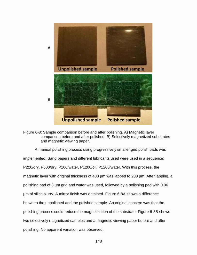
148

Figure 6-8: Sample comparison before and after polishing. A) Magnetic layer comparison before and after polished. B) Selectively magnetized substrates and magnetic viewing paper.

A manual polishing process using progressively smaller grid polish pads was

implemented. Sand papers and different lubricants used were used in a sequence:

P220/dry, P500/dry, P100/water, P1200/oil, P1200/water. With this process, the

magnetic layer with original thickness of 400 µm was lapped to 280 µm. After lapping, a

polishing pad of 3 µm grid and water was used, followed by a polishing pad with 0.06

µm of silica slurry. A mirror finish was obtained. Figure 6-8A shows a difference

between the unpolished and the polished sample. An original concern was that the

polishing process could reduce the magnetization of the substrate. Figure 6-8B shows

two selectively magnetized samples and a magnetic viewing paper before and after

polishing. No apparent variation was observed.

Unpolished sample Polished sample

Unpolished sample Polished sample

A

B

149

Some magnetic imperfection over the surface of the magnet were observed

during the magneto optical image of the selectively magnetized samples, even after

polishing. These imperfections were originally attributed to material roughness;

therefore, roughness characterization was conducted. Results are presented in Figure

6-9 showing microscopy images of the surface and cross-section (after cleaving).

Figure 6-9: Optical microscopy image of the BJA magnet surface, top view and cleaved cross section. Magneto optical image at the surface of a selectively magnetized sample (similar image for polished and unpolished samples).

Magneto optical images of a selectively magnetized sample were taken before

and after polishing and magnetic fields remain almost the same (right image in Figure 6-

9). This confirms that the magnetic imperfections were not produced by the material

roughness and suggest that the selectively magnetization process is not completely

magnetizing the poles on the substrate. This gives evidence that there is still room for

improvement on the selective magnetization process.

To accurately evaluate the effectiveness of the polishing, two samples (polished

and unpolished) were analyzed using an optical profilometer (Bruker, Contour GT-I).

150

The unpolished sample has an average Ra=770 nm (surface roughness), while the

polished sample Ra=20. Results presented in Figure 6-10.

Figure 6-10: Optical profilometer image of polished and unpolished 3 mm × 3 mm magnet (BJA).

From these results, it is concluded that NdFeB magnets grade N42 provided by

BJA, are the best candidates to be a substrate in the mass fabrication of magnetic

bases for levitated microrobots. To the date of this research, this is the material that

offers higher magnetic energy product, lower thickness and better qualities for

machining.

6.3 Adapting Selective Magnetization for Microrobot Bases

As explained in Chapter 4 of this document, selective magnetization is a

technique to reverse the magnetization of selected areas of a magnet by “imprinting”

magnetic patterns using a magnetization mask meanwhile a reversal field is applied.

This process is ideal for the batch fabrication of the robot bases with checkerboard

magnetic patterns, because it will eliminate the manual assembly of individual 1 mm x

1 mm square magnets. Manual assembly is difficult and time consuming due to

attractive and repelling forces of the magnets.

151

6.3.1 Improving Magnetization: Simulations

The selective magnetization process was simulated using COMSOL multiphysics

(2D quasi-static simulations in COMSOL), as described in section 4.2.1. These

simulations provide a fast evaluation mechanism for different design parameters. The

first parameter to be evaluated is the mask material. Different soft ferromagnetic

materials will have different saturation magnetization. A higher saturation magnetization

will produce a higher magnetic field underneath the mask during the reversal

magnetization. The hypothesis is that higher magnetic field under the mask will result in

an increase of magnetic contrast (defined as C=(Bmax-Bmin)/(Bmax+Bmin)), therefore the

magnetic patterns quality will be improved.

During section 4.2.1. Carbon steel was used to magnetize flexible iron oxide (at

0.5 T). The saturation magnetization of the carbon steel was not a limiting factor, but the

magnetic substrate (NdFeB) requires a high reversal magnetic field of ~1.5 T. By

simulating the magnetization process at different reversal fields and measured the peak

magnetic field underneath a simple 1 mm x 1 mm square mask, it is possible to

compare the effectiveness of different mask materials. Figure 6-11, compares the

magnetic field produced underneath masks fabricated with 2V permendur,

supermendur, low carbon steel 1018, and permalloy. The magnetic properties for these

various materials were from the COMSOL library and/or measured in the laboratory.

The reversal magnetic fields used during selective magnetization are highlighted.

152

Figure 6-11: Set of materials to take into consideration for the magnetization mask fabrication.

Although it is possible to increase the reversal magnetic field underneath the

mask by selecting a different material such as supermendur or 2V permendur rather

than carbon steel, the reality is that this increment (9% for 2V permendur and 6% for

supermendur) does not worth the extra cost and difficult machinability of these two

materials for this project. Therefore, carbon steel will continue to be the designated

material for the mask.

Variations on the mask thickness were also simulated. The magnetic contrast will

be used as figure of merit. Figure 6-12 confirms that it necessary to fabricate thicker

masks to increase magnetic fields. Increasing the fields will generate better magnetic

patterns with sharper edges. Simulations indicated that a minimum aspect ratio (mask

pole height / pole width) of 3 is necessary for achieving good magnetic contrast.

153

Figure 6-12:Selective magnetization simulation model. A) COMSOL simulations of Bz field generated by a magnetization mask, parametric with thickness. B) Contrast calculation for different mask thickness (at the middle section of the magnet).

Another important parameter that was simulated was the importance of using

one magnetization mask in comparison with two aligned magnetization masks (beneath

and underneath the magnetic substrate). Comparative simulations are presented in

Figure 6-13A. Double mask showed better performance in terms of magnetic contrast

underneath the patters. It is easy to appreciate how strong and uniform is the magnetic

field (across the thickness of the magnet) when using double mask. A numeric

comparison of the magnetic field at the center of the magnet is presented in Figure 6-

13B. Double mask generates a higher magnetic contrast underneath the mask features.

Field dependency with mask thickness

minmax

minmax

BB

BBC

Last machined mask thickness

Mas

k th

ickn

ess

A B

154

Figure 6-13: Selective magnetization simulation model, double mask. A) Simulation comparison for single and double mask with magnet on the middle. B) Comparison of the magnetic field along the center of the magnet for single and double mask. External applied field Bext= 1. 5 T.

6.3.2 Improving Magnetization: Field Selection

The following steps will describe variation process for the selective magnetization

procedure and experiments conducted after selecting carbon steel as material for the

magnetization mask. To have a better control over the applied magnetic field and to

reduce Eddy currents during the magnetization (that could potentially reduce the total

magnetization of the sample), we proposed to use DC magnetic field instead of a pulse

magnetizer. We used a vibrating sample magnetometer (VSM – ADE technologies) to

generate the external reversal field.

Considering the DC-demagnetization curve of the substrate for the magnetic

bases (NdFeB), we compared three reversal fields (1 T, 1.5 T and 2 T). A magnetization

mask with stripe-like patterns and pole width of 1 mm was used for the experiment.

Figure 6-14 present MOI measurements of the substrate after selective magnetization

of the three reversal fields, confirming that ~1.5 T will be the best reversal field to obtain

Bext = 1.5 T Dt= 1 mm Single mask over magnet

Double mask: Magnet in the middle

Bext =1.5 T \ Dt =1mm

Single

Double

-3

-2

-1

-1.2

-1.4

-1.6

-1.8

-2.2

-2.4

-2.6

-2.8

By

fiel

d [

T]

-3 -2 -1 0 1 2 3Distance [mm]

Mask

Magnet

Dt

Dt

Magnet

Mask

Mask

Single mask over magnet


2.5

2.0

1.5

1.0

|B|[T]

Mask

Magnet

Dt

Dt

Magnet

Mask

Mask



Mask

Magnet

Dt

Dt

Magnet

Mask

Mask



Mask

Magnet

Dt

Dt

Magnet

Mask

Mask



-3

-2

-1

0

1

2

-5 -4 -3 -2 -1 0 1 2 3 4 5Distance [mm]

Dis

tan

ce [

mm

]

Double maskSingle mask

Mask

Magnet

Dt

Dt

Magnet

Mask

Mask



BA

155

magnetic pole patterns of the same size and fields with the same absolute value

(symmetric magnetization pattern with positive magnetic field equal to the negative

magnetic field).

Figure 6-14: DC magnetization of lines, varying the applied magnetic field. MOI measurements at 500 µm from surface.

6.4 The Magnetization Mask

6.4.1 Mask Fabrication Exploration

The most important job is to fabricate the magnetization mask. This should be

accomplished after defining geometry parameters, magnetization mask material and

reversal field to be applied during the selective magnetization process. The mask

fabrication is a critical step towards obtaining multiple magnetic bases from a single

magnetic substrate (batch-fabrication). The first set of magnetization masks was

designed to magnetize four robots (each one as an array of 3x3 alternated poles of

1 mm side) in the same substrate.

2 T 1.5 T 1 T

Magnetizing lines: Measures at 500 µm from surfaceX displacement [µm]Y

dis

pla

cem

ent

[µm

]

156

Figure 6-15: (Top) Mask fabrication initial exploration with a batch of four robots per mask. Mask design alternatives using different commercial CNC end mills and drill bits. (Bottom) Final machined masks.

As presented in the top row of Figure 6-15, four variations were made on the

mask: Mask 1_1 was designed with squares made with a 1/64” commercial end mill;

Mask 1_2_1 and Mask 1_2_2 were made with simple circles using 1/32” end mill and

1mm drill bit respectively, and Mask 1_3 was made with simple circles using 1/64” end

mill. All masks were made from the same material (AISI 1018 mild/low carbon steel).

Top row on Figure 6-15 shows schematics and bottom row presents pictures of the

resulting masks.

Mask 1_1 Square structures

Mask 1_2_1 End-mill circle structures

Mac

hin

ed m

ask

pic

ture

Mask 1_2_2 Drill-bit circle structures

Mask 1_3 Small circle structures

157

Figure 6-16: Magneto optical images measured at 50 µm of magnetized samples. Samples magnetized using the same field (1.5 T) and four different masks. Bz comparison for substrates at similar height (200 µm) but different mask. The manually assembled 2x2 magnet array was also measured and compared (SRI sample in green).

Samples were magnetized using different masks. The substrates in this

experiment were 4.9 mm x 4.9 mm x 0.7 mm NdFeB magnets. The reversal magnetic

field was 1.5 T. Individual 3x3 bases were not diced for this experiment. Figure 6-16

summarizes the stray magnetic field (Bz) measured using magneto optical images at

50 µm from surface. Additional measurement (200 µm from surface) of a manually

assembled magnetic base was included for comparison (2x2 magnet array sample

provided by SRI – line in green). The results look promising; Bz fields are in the same

order of magnitude for most of the masks (except small 1/64” circles mask that remains

lower).

X 10-3

Squares

Circles 1 mm

Circles 1/32”

Circles 1/64”

SRI 2x2 (@250 µm)@250 µm





X 10-3

Squares

Circles 1 mm

Circles 1/32”

Circles 1/64”

SRI 2x2 (@250 µm)@250 µm

Squares

Circles 1mm

Circles 1/32”

Circles 1/64”SRI @250 µm

X 10-3

Squares

Circles 1 mm

Circles 1/32”

Circles 1/64”

SRI 2x2 (@250 µm)@250 µm





X 10-3

X 10-3

Squares

Circles 1 mm

Circles 1/32”

Circles 1/64”

SRI 2x2 (@250 µm)@250 µm





X 10-3

X 10-3

Squares

Circles 1 mm

Circles 1/32”

Circles 1/64”

SRI 2x2 (@250 µm)@250 µm





X 10-3

X 10-3

Squares

Circles 1 mm

Circles 1/32”

Circles 1/64”

SRI 2x2 (@250 µm)@250 µm





X 10-3

500 µm

Bz

fiel

d [

mT]

Distance [µm]

Circles 1/64”Squares

Circles 1/32” Circles 1 mm

158

6.4.2 Low Aspect Ratio Magnetization Mask

The aspect ratio of the mask will be designated as the thickness over feature

length. If a square with 1 mm side and 1 mm depth is machined, then the aspect ratio

will be 1. A square patter mask was selected to complain with the specifications of the

microfactory base. Differing from design in Figure 6-15, all the robots have the same

magnetic pattern. Resulting magnetic square poles at individual bases should have

1 mm side. A total of 9 magnetic bases (3 mm x 3 mm) can be fabricated in the selected

10 mm x 10 mm substrate. Robot distribution over a substrate is presented in Figure 6-

17A. With this distribution, it will take 22 substrates to fabricate 200 robots.

As mentioned in section 6.3.1, it was clear that the next step was to design and

fabricate a double side magnetization mask. Technical drawings were made using solid

works. Figure 6-17B shows the desired pattern and the 3D model of one side of the

mask.

Figure 6-17: Modeling the log aspect ratio mask. A) Desired pattern for batch fabrication of 9 micro-robots per substrate. B) 3D representation of the magnetization mask to generate the desired pattern.

The complete mask was designed as sandwich of two identical patterned masks,

made of carbon steel (AISI 1018 mild/low carbon steel - ASTM A108). All mask features

(a) (b)A B

159

are 1 mm depth (feature in the mask will have an aspect ratio of 1). In the middle, a zinc

spacer was designed to align the magnetic layer. Figure 6-18A shows and explosion

schematic of the mask. The three parts of the mask and the magnetic layer will hold

together using three wood alignment pins. This mask was machined using a Sherline

2000 CNC and 1/64”-two flutes end mills. Figure 6-18B shows the final machined mask

disassembled.

Figure 6-18: Model and fabrication of double side mask. A) Schematic of the double side magnetization mask used to produce 9 micro-robots. B) Fabricated magnetization mask (disassembled).

6.4.3 High Aspect Ratio Magnetization Mask

As mentioned in Figure 6-12, the higher the aspect ratio of the mask the better

magnetic field quality will be generated during the reversal magnetization. With this

premise in mind, it is necessary to fabricate different magnetization masks, but this

raises a fabrication problem. It is very complicated to machine carbon steel with high

aspect ratios using dimensions smaller than 1 mm. Commercial end-mills smaller than

1/64” are limited to 1 mm length.

Zinc spacer

(a) (b)A B

160

A laminated design was proposed to obtain high aspect ratios: Use the CNC or

laser cut to machine individual layers out of 1 mm thick carbon steel sheets (two

different designs of layers, one with 6 x 1 mm3 poles and other with 3 x 1 mm3 poles to

create the checkerboard). This process will generate perfect square shape angles in the

features and the most important, controllable aspect rations higher than 10. After three

layers are machined, they will be glued together in rows (6/3/6 pole layer) and three

rows will be glued with a 300 µm spacer between them, as shown in Figure 6-19. This

fabrication concept was originally tested using laser cur over stainless steel (easier to

machine) and then implemented in carbon steel using CNC. As shown in Figure 6-19C,

the saturation magnetization of stainless steel is lower than the carbon steel.

Figure 6-19: Laminated mask approach. A) 3D design of the mask and CNC program to produce every layer of the mask. B) Laser machined stainless steel mask C) VSM measurement comparison of low carbon steel (CNC), stainless steel (laser cut) and NdFeB (BJA) magnet.

The optimal reversal magnetic field for the high and low aspect ratio masks are

different. Both high aspect ratio masks (stainless steel and carbon steel) were used to

magnetize individual magnetic bases (3 mm × 3 mm x 0.4 mm). Variations on the

reversal magnetic field were made to find the optimal magnetization (higher contrast).

A

CNC program to machine

both parts of mask

B

-2.5

-2.0

-1.5

-1.0

-0.5

0.0

0.5

1.0

1.5

2.0

2.5

-2.0 -1.5 -1.0 -0.5 0.0 0.5 1.0 1.5 2.0

µo·M

[T]

µo·H field [T]

Low Carbon Steel

Stainless Steel

NdFeB (BJA)

C

161

For these two masks the best external magnetic field was selected as 1T, as shown in

Figure 6-20.

Figure 6-20: Finding the right external magnetic field used during the selective magnetization. Stainless steel and carbon steel masks.

A comparison of three substrates magnetized with the fabricated masks is

presented in Figure 6-21. Contrary to expectations, the high aspect ratio did not provide

significant improvement over the low aspect ratio mask. Even though the shape of the

Stainless steel (laser cut) Low carbon steel (CNC)

-100

-80

-60

-40

-20

0

20

40

60

80

100

-1 -0.5 0 0.5 1

B f

ield

[m

T]

Distance [mm]

Bext = 1.6 T

Bext = 1.4 T

Bext = 1.2 T

Bext = 1.0 T

-100

-80

-60

-40

-20

0

20

40

60

80

100

-1 -0.5 0 0.5 1

B f

ield

[m

T]

Distance [mm]

Bext = 1.5 T

Bext = 1.3 T

Bext = 1.0 T

162

magnetization pattern was improved, the absolute values of the magnetic fields

produced by the selectively magnetized arrays were not significantly different.

Figure 6-21: Magneto optical image of a selectively magnetized samples using each of the machined masks. Measured at 500 µm from magnet surface. S1 corresponds to low aspect ratio carbon steel, S2 is the high aspect ratio, laser cut stainless steel, and S3 is the high aspect ratio CNC machined.

To understand the discrepancy between the results using low and high aspect

ratio masks, it was necessary to generate a 3D simulation model (2D simulations have

been used so far), as depicted in Figure 6-22. We simulated the magnetic fields

generated between two (aligned) high aspect ratio masks, separated by an air gap of

400 µm, in a constant external magnetic field of 1 T over the z-axis (to simulate pulse

magnetizer and VSM). Under these circumstances we observed that the difference of

magnetic field between exposed and unexposed areas (by the mask) was only 600 mT.

Generating a very low magnetic contrast ~0.2. We then noticed that unexposed areas

were experiencing very high fields contributing to reversing the overall magnetization of

the sample.

To overcome these difficulties and to increase the magnetic contrast during the

selective magnetization process, results in a task that exceeds the scope of this project.

Future development on this specific area will be described at the end of this dissertation

in Chapter 9. To advance with the batch fabrication of magnetic bases, the only

-50-40-30-20-10

01020304050

-1.2 -0.8 -0.4 0 0.4 0.8 1.2

B f

ield

[m

T]

Distance [mm]

UF 1stUF 2ndUF 3th

S1: Low aspect ratio

carbon steel

S2:High aspect ratio

stainless steel

S2:High aspect ratio

carbon steelS1

(1.0 T) (1.5 T) (1.5 T)

S2S3

163

magnetization mask that will be used hereafter is the double side low aspect ratio

presented in Figure 6-18.

Figure 6-22: 3D simulation of the laminated mask (double mask) under permanent external B field. External field = 1 T. A) Perspective view, B) horizontal cross section in the middle of the air gap, and C) Bz field measurement.

6.5 Characterization of Microrobot Bases

Using selective magnetization process to create magnetic bases (at 1 T reversal

field), the following results are presented: Figure 6-23 shows the magnetization of the

BJA magnetic layer using the machined double mask. Two magneto optical image

techniques were used: A) and B) were obtained using magneto optical (MO) sensor of

38 mT saturation field in the “Minimo” magnetic camera (Matesy). These pictures show

a manually assembled 3x3 magnetic bases, a selectively magnetized base, and the

entire substrate (10 mm x 10 mm x 0.4 mm) before being singulated. The images are

crisper and the magnetic poles are well defined, because the magnetic sensor saturates

at magnetic fields lower than the produced by the magnets. This images confirms that

the selectively magnetization process is not fully magnetizing the alternated poles.

Figure 6-23C is using the magneto optical image developed in Dr. David Arnold’s group

[133]. The advantage of this technique is that the intensity of the magnetic field can be

quantified. The magneto optical image taken at 500 µm from the substrate was

A B C

164

superpose over the micrograph image of the substrate to demonstrate the success of

selectively magnetization process.

Figure 6-23: Magneto optical image of the selective magnetization of BJA substrates. A) Comparison between manually assembled and selectively magnetized bases. B) Selectively magnetized substrate containing 9 robots (before dicing). C) In house magneto optical image, superpose over a micrograph of the magnetic substrate.

By quantifying the stray magnetic field from the magneto optical image, a

comparison between manually assembled micro-robots and selectively magnetized

micro-robots is presented in Figure 6-24. These measurements show the B field peaks,

obtained from the selectively magnetized samples (~50 mT maximum) are about 50%

weaker than the manually assembled robot (~100 mT maximum).

Manually assembled robot

Selectively magnetized robot

Selectively magnetized BJA substrate(10 mm x 10 mm)

Magneto Optical Image

1 mm

North pole South pole

Magnetic Layer

A B C

165

Figure 6-24: MOI measures. Assembled and selectively magnetized levitated micro-robot’s comparison. Measurements at 600 µm.

Two batches of magnetic bases were fully produced. A ~280 µm and a ~400 µm

thick batches, with 9 bases each. Figure 6-25 shows the fabrication results. The

fabrication process can be summarized in the following steps:

• Lapping one side of a commercial 10 mm x 10 mm x 0.4 mm NdFeB magnetic substrate, to obtain a designated thickness.

• Polishing the lapped side to obtain mirror finish.

• Fully magnetize the substrate up (7T).

• Reverse magnetization using low aspect ratio, carbon steel double side mask (1.2 T).

• Substrate singulation into nine micro-robot bases using dicing saw.

• Manually cleaned, separation and packaging.

Manually assembled 3x3 magnets micro-robots

Magnetized and not diced (double mask)

500 μm 500 μm

Measurement

MOI measurements at 600 μm

Measurement

-200 -150 -100 -50 0 50 100 150 200B field [mT]

Manually assembled

Selectively magnetized

166

Figure 6-25: Fabrication of nine micro-robots per batch. A) None polished magnetic base after dicing, with a magneto optical image (MOI) inset of one of the base. B) Singulated and polished robots ready for shipping.

The stray magnetic field of each base was measured using magneto optical

imaging technique and presented in Figure 6-26, for evaluation of the process

reproducibility.

Figure 6-26: MOI characterization of samples from the same batch (280 µm thickness). A) Images obtained at 500 µm from surface. B) Quantification of the B field cross section for all robots in the batch.

3 mm

A B

400 μm thick

280 μm thick

MOI inset

1 3 5

A

C

E

A1 A3 A5 C1 C3 C5 E1 E3

Measurement height: 500 µm

BA

167

An additional stray magnetic field characterization technique was used to validate

results: scanning hall probe. Figure 6-27 depicts an example of this characterization

technique by comparing a manually assembled robot with a batch-fabricated one.

Scanning hall probe confirms that selective magnetization of 280 µm thick substrates

generates patterns with only ~39% of the magnetic field strength of the manually

assembled patterns.

Figure 6-27: Scanning hall probe measurements of manually assembled and selectively magnetized sample.

The final goal of the micro-robots is the diamagnetic levitation of their own

masses plus a payload. In this order of ideas, we studied the diamagnetic force

generated for three samples: a manually assembled robot, a selectively magnetized

X displacement (mm)

B f

ield

(mT)

Man

ual

ly a

ssem

ble

d S

RI s

amp

le

(sen

sor

at s

urf

ace)

Max field139.8 mT

Min field-140.7 mT

Plot line

X displacement (mm)

B f

ield

(mT)

Sele

ctiv

ely

mag

net

ize

sam

ple

(sen

sor

at s

urf

ace

)

Max field54.5 mT

Min field-51.2 mT

280 µm thickness

168

400 µm thick robot and a 280 µm thick robot. We used a combination of a microbalance

(Explorer 2, Ohaus) and a polished pyrolytic graphite as a sensing mechanism, as a

variation of experiment conducted by [239]. Each sample was attached to a glass and

plastic sample holder facing the graphite and connected the holder using a stiff brass

beam with a 3D micro positioner (build on house with Newport DC servo controllers). By

cautiously lowering the magnet on top of the graphite, the repelling diamagnetic

levitation force will push the graphite away and we will register this force as weigh in the

balance. Figure 6-28 illustrate the experiment and results.

Figure 6-28C compares measurements of the magnetic force with COMSOL

simulations and charge model calculations (as presented in section 3.4). A factor of

0.35 and 2.8 (simulation and analytic model) are used arbitrarily to compensate

variations on material properties for the specific samples. Differences in the slope of the

manually assembled base compared with models are attributed to instrumentation error.

It is clear from Figure 6-28C that the force produced by the manually assembled

base is higher than its own weight (red curve). On the other hand, the force produced by

400 µm thick selectively magnetized bases is slightly smaller than their own weights,

and therefore it won’t levitate. Similar behavior occurs with the 280 µm thick bases, but

the produced force is considerably lower. Enhancing the magnetic field produced by the

selective magnetization will increase the diamagnetic force and overcome the weight of

the magnet making the micro-robot levitate.

169

Figure 6-28: Diamagnetic force measurement using a microbalance. A) General assembly, B) close-up of sample holder and C) force measurement results.

Although the selectively magnetized fields and the diamagnetic forces are

weaker than the manually assembled counterparts, experiments conducted using SRI

microfactory (Figure 6-29) verify that this technique can in fact fabricate microrobots to

perform assisted levitation (diamagnetic levitation biased by an additional external

magnetic field) and assisted magnetic sliding (using the microfactory platform to

displace bases, achieved by controlled electric currents and diamagnetic layer).

Figure 6-29: Characterization of batch fabricated robots at SRI. Left, assisted levitation and right, assisted sliding.

Glass

3 axis micro-

positioner

Scale (resolution μg)

Measurement assembly:

Sample holder

arm

pyrolytic graphite

ScaleSample

Sample holder arm

A B C

Dash lines: Magnetic base weight

Levitation region for 400 µm thick bases

10

100

1000

0 200 400 600 800

Dia

mag

net

ic F

orc

e [µ

N]

Distance [µm]

SimulationAnalyticManually assem.UF_400µmUF_280µm

170

6.6 Summary

A batch fabrication of monolithic magnetic bases for microrobots was

successfully obtained. Selective magnetization was used to imprint alternated magnetic

pole patterns in a machinable NdFeB substrate, producing 9 microrobots per batch.

Two types of magnetization mask were explored (low and high magnetization) showing

similar results among them. The diamagnetic repelling force of bases with two thickness

(400 µm and 280 µm) was measured showing that the thicker base produced higher

force. Enthought the fabricate bases don’t self-levitate, they were capable of assisted

levitation (external magnetic field bias) and operation in sliding mode (lateral movement

using microfactory platform).

171

CHAPTER 7 ADDING FUNCTIONALITY TO MICROROBOTS: END EFFECTORS*

A common challenge for microrobotic platforms is adding more functionality [13]

and the need of fixturing and gripping strategies [241] to better interact with external

micro-parts. Most of the strategies used to address this problem rely on some form of

microgrippers [242], [243], [244] that are very difficult to customize because of the

system complexity. However, there are many microrobotic manipulation tasks that do

not require grabbing, such as dispensing droplets and micropositioning, which are the

target of this work.

The primary solution for enabling multi-functional interactions in macroscale

robotics is the use of end effectors. An end effector is the protrusion of a robot intended

to interact with the environment and perform a task. This end effector can be fixed or

replaceable, and translating this concept to the field of micro/milli robotics is of high

interest. In small scales, there is the same need for simple, task-specific end effectors

[245] that can be exchangeable for addressing different tasks (i.e. pick and place,

scanning surfaces) or interacting with objects with different properties (i.e. solids,

liquids, different sizes). Fabrication techniques capable to create end effectors with

micrometer resolution features will bridge the gap between millirobots and micro-part

assembly. Exchangeability is also desirable in case of damage or part wear.

Wafer-level microfabrication is desirable for realization of hundreds or thousands

of microrobots that can complete complex tasks by working in parallel, such as

“microfactory” or “swarm” concepts. Because magnetic actuation is fairly common for

* This section contains excerpts from reference [240].

172

micro/milli robots [40], [46], [246] and based on the successful advances in functionality,

complexity and reproducibility developed by SRI International [110], [235], the end

effectors developed here are designed for compatibility with these magnet-array

microrobot platforms operating under the diamagnetic levitation principle. However, the

general concepts presented here could be modified for other microrobotic platforms.

Previews attempts of end effectors used by SRI international in their levitated

microrobots were described at [247]. Those attempts included tungsten wires

(electrochemically etched), polyamide (photolithography) and a combination of

polyimide and soft elastomer styrene-butadiene-styrene -SBS- (dip-coated). The former

one used to increase the surface area upon contact and the pick strength of the end

effector. In Figure 7-1, commercial end effectors are compared with an electroplated

end effector fabricated following procedures described in this chapter. The primary

parameter for maintaining the microrobot’s levitation is that the mass of the end effector

should be <5% of the robot’s mass.

Figure 7-1: Comparison between fabricated end effector (Copper) and commercially available end effectors: tungsten wire, polyamide and a combination of polyamide and SBS elastomer [247].

A microfabrication process for batch production of magnetically attached

(exchangeable) end effectors for micro/milli robots is describe in this chapter. The end

effectors make use of soft ferromagnetic materials to enable interchangeable and

173

adjustable attachment to magnetic bonding surfaces on robotic bases. The end

effectors have overall dimensions in the millimeter scale (8 mm and 7 mm length), but

employ microstructured tools (eight shapes) for manipulation of objects below 10 µm

with micro and nano scale precision. Three materials—copper, nickel and SU-8—are

used for forming the end effector body, and nickel is used as the magnetic attachment

material in all cases. An additional fabrication method called hybrid produced end

effectors with nickel body and tips made of SU-8. The end effectors are assembled onto

diamagnetically levitated microrobot bases in order to demonstrate the versatility of the

exchangeable end effector technology.

7.1 End-effector Design and Fabrication

7.1.1 Design Considerations

A first goal for the end effector is to enable task-specific function, while

minimizing the weight (payload) of the end effector. Another long-term goal is to provide

for multiple functionalities (electrical, mechanical, thermal, etc.), so three types of

materials are considered for the main end effector body: a non-magnetic metal (copper),

a ferromagnetic material (nickel), and a dielectric material (SU-8 photo-patternable

epoxy). A comparison of each material’s Young’s modulus, density and weight (based

on end effectors fabricated for 3x3 and 4x4 magnets arrays) is presented in Table 7-1.

Even though SU-8 is the lighter material, it also has a lower Young’s modulus, making it

less rigid and potentially mechanically unstable for long thin end effectors.

Table 7-1. End effector material properties.

Material Young's modulus

[GPa] Density [g/cm3]

Mass (3x3) [μg]

Mass (4x4) [μg]

Nickel 220 8.9 140 283

Copper 117 8.9 140 284

SU-8 2 1.2 19 38

174

In the case of the SRI microrobots, the stray fields from the magnetic base are

used to attach end effectors without affecting the properties or function of the robot

base. Since the microrobot base is an array of permanent magnets, soft ferromagnetic

nickel is incorporated in the end effector enabling it to easily and reversibly snap onto

the base. To enable attachment to other types of microrobots, permanent magnet

materials could be used instead of nickel.

The microfactory concept involves multiple robots, potentially working in close

proximity to one other and even co-manipulating the same part. To avoid unwanted

attractive forces between magnetic bases, the end effectors are designed with shanks

that protrude at least 2 mm away from the base. Additionally, in order to manipulate

objects smaller than 10 µm, finely shaped, high-precision end effectors are required

(~10 µm). Together, these requirements demand fabrication of long, slender structures,

which can be prone to bending. Consequently, the mechanical robustness of the long

end effectors is a key area for investigation. Figure 7-2 shows an end effector (nickel)

magnetically attached to the magnetic base (here, a 2 x 2 array of permanent magnets).

End effectors are designed to have the center of mass at the same x and y position as

the center of mass of the magnetic base. Two sizes of end effectors are developed: 7.1

mm and 8.6 mm in overall length (for 3 x 3 and 4 x 4 magnet bases with 2 mm shank).

175

Figure 7-2: Microfabricated end effector assembled on a magnetic base. A) Schematic of the assembly. B) Fabricated microrobot. Body made of ~2.6 µm thick nickel. Close-up of the end effector tip to show the interaction surface with 17 µm diameter.

7.1.2 Fabrication

Two generations of end effectors were proposed: In the first generation, the end

effector (containing magnetic attachment features) and the tip are fabricated in the

same material. In the second generation, the end effector and the tip are fabricated with

different materials, therefore it will be called hybrid.

First generation: Single material for end effector and tip

To enable heterogeneous integration of multiple materials (one for magnetic

attachment, the other for the main structure), a two-step fabrication process is used.

The first step employs electroplating to form the nickel magnetic attachment structures,

and the second step forms the shank and tool tip. Figure 7-3 shows cross-section

schematics of the three different materials.

Nickel magnetic attachment

Manually assembled magnetic base

1 mm

Nickel end effector

17 μm

Tip

B

End effector body

Magnetic base

Magnetic attachment

A

176

Figure 7-3: Cross section schematic and layer thicknesses of the three different end effector types: copper, nickel and SU-8 (not drawn to scale).

For the first step, a seed layer of Ti/Cu (100 nm/50 nm) is sputtered (Multi-

Source RF and DC Sputter System CMS-18, Kurt J. Leskar), 9.5-µm-thick photoresist

(AZ9260) is patterned using a first lithography mask, and a ~2.5 µm nickel layer is

electroplated using a commercial bath (Nickel Sulfamate RTU, 33 mA/cm2 current

density, nickel anode). The Ti layer serves as adhesion layer between the Cu and the Si

during the electroplating and also serves as a sacrificial layer during the releasing step.

In the second step, the process flow depends on the material. For the Cu and Ni

structures electroplating is again used, so it is necessary to sputter a second seed layer

of Ti/Cu (100 nm/50 nm) on top of the existing features. An ~8-µm-thick photoresist

(AZ9260) is photo-patterned with a second lithography mask, and the metal (Cu or Ni) is

electroplated. Cu uses a solution of copper (II) sulfate pentahydrate and sulfuric acid

(10 mA/cm2 current density, copper anode). Ni uses the same bath conditions as

177

before. Alternatively, the SU-8 end effectors are made by spin coating OmniCoatTM

(MicroChem) and a ~10 µm layer of SU-8 over the sample, followed by lithographic

patterning. For all three materials, the final structures are released from the substrate by

dissolving the Ti/Cu seed layer in a bath of ammonium hydroxide saturated with copper

sulfate (blue etch) [etches Cu] followed by hydrofluoric acid (HF) [etches Ti].

Second generation: Hybrid materials for end effector and tip

For the second generation of end effectors the fabrication process is divided in

two main layers (therefore 2 lithography masks): (1) The first layer form a nickel end

effector body that was electroplated. (2) The second layer is intended to produce the

tips and tethers that support the end effectors and it was fabricate by spin coating SU-8.

Both layers were produced following procedures described in the first generation

of end effectors, except for the structure release were different sacrificial layers were

used. Two sacrificial layers were compared during this generation: Titanium and LOR

3A (polymeric lift off resist by MicroChem). A cross section comparison of both

sacrificial layers before releasing is presented in Figure 7-4A. The reason to eliminate Ti

as a sacrificial layer, is to avoid using hydrochloric acid and improve the quality of the

produced structures (prolonged exposures to HCl will swallow the SU-8). A polymeric

sacrificial layer will also speed up the releasing process and increment the yield of the

produced structures.

It is important to mention that second generation of end effectors will not have

additional magnetic attachment structures because the entire body is made of nickel,

simplifying the fabrication and reducing one lithographic mask. Cross section and top

view schematics of the end effector after release are presented in Figure 7-4B. Final

178

recipe used to produce the first layer of end effectors (second generation) is presented

in Figure 7-5 and the second layer is presented in Figure 7-6.

Figure 7-4: End effector fabrication schematics. A) Cross section schematic of the materials for the end effector body (no SU-8), before releasing. Comparisons of two sacrificial layers: Ti and LOR. B) Schematic of the hybrid end effectors after release, were the tip is made of SU-8 and the body of nickel.

BA

Cu seed layer Nickel SU-8

Hybrid end effector:

Nickel - electroplated

Cross section

Top view

Nickel - electroplated

SU-8

179

Figure 7-5: Fabrication recipe for hybrid (Nickel + SU-8) end effector with LOR as a sacrificial layer. First layer: the nickel electroplated end effector body.

Substrate Name: A2P_EE_M2_01

Material / Type / Orientation: Silicon / N type / <100>

Wafer Diameter / Thickness: 100 mm / 500 µm

PO# / Lot: PO# 437422 / Lot 3115

1Step Procedure Parameter Value

1.1 Si Wafer cleaning PRS 3000 bath at 70ºC for 3 minutes in solvent bench

Triple water rinse in solvent bench

Ni blow

BOE etch for 30 sec in acid bench

Water rinse in acid bench

Ni blow

Asher treatment for: 300 w, 300 s, O2 at 600 sccm, ~1200 mtorr (Anatech Barrel SCE600)

1.2 Coat LOR 3A layer (aprox 700nm) Dispense dinamic, covering 90% of wafer in Laurel spinner - Manual mode

Spread during dispense at 600rpm, Aceleration: 130 (as soon as dispensed change step)

Spin for 45 sec, 600rpm, Aceleration: 145

Bake for 30min in Despatch oven at 170ºC

1.3 Seed layer deposition (Cu) Mount wafer and glass slide (half area protected with kapton tape) in sputter holder

Deposit 200 nm of Cu using sputter deposition- (KJL CMS-18 Multi-Source) Dwell time (s) 417

Source 3

Measure seed layer thickness using profilometer over glass slide (Dektak 150) Thickness (nm)

1.4 AZ9260 [+] patterning (~ 10 µm) HMDS treatment (hot plate 3 min / HMDS 30 s / hot plate 2:30 min / out side 30 s)

Spin coat ~10 µm AZ9260 using recipe LP_9260_10.13 / Tall ring (Suss Delta 80 spinner)

Mask name: Bake for 3 min in hot plate at 112ºC. Rehydrate for 24 min

A2P_EE_M2_L1 Expose mask, hard contact, Algap=50 µm and wec =0 (Karl Suss MA6) Lamp (mW/cm^2) 7.1

Time (s) = Dose(mJ/cm^2) / Energy (mW/cm^2) => Dose @ 10 µm = 720 mJ/cm^2 Expose time (s) 101.41

Prepare 3:1 (H2O:AZ400K) solution (75 ml DI: 25 ml AZ400K) at room temperature

Develop AZ400K (4:1) solution for 5:30 min under agitation Develop time (m) 5:30

Stop process immersing in DI water for 30sec, stir


Measure photoresist thickness using profilometer on test area (Dektak 150) Thickness (µm)

1.5 Ni electroplating (~2.5 µm) Prepare Nickel Sulfamate RTU (Techni nickel S) over hotplate: 100 rpm / 54ºC / temperature probe

Connect nickel electrode in the positive (+) terminal

Prepare power supply for 33 mA/cm^2 current density (DuPR10-.1-.3) Area (cm^2)

Current (mA) = Current density (mA/cm^2)* Area (cm^2) Set current (mA)

Remove Cu oxide usign 1:10 (HCl:H2O) 30 s under agitation

Rinse with water for 1 min

Ni blow

Assemble wafer in the holder and connect to negative (-) terminal

Turn on current in the power supply

Measure pH: 3-4.5 (Optimal: 3.8) pH

Insert wafer in the bath and electroplate for 20 min Time (m) 20

Deposition rate = ~0.65µm/min @ 33 mA/cm^2 Current m. (mA)

Voltage m. (V)

Measure pH pH

Remove sample and turn off current in the power supply

Rinse with water

Strip photoresist with acetone

Isopropanol (IPA) rinse

Ni blow

Measure Ni thickness using profilometer on test area (Tencor AS500) Thickness (µm)




Ni blow


Bake for 3 min in hot plate at 112ºC. Rehydrate for 24 min

2.2 Coat OmniCoat HMDS treatment (hot plate 3 min / HMDS 30 s / hot plate 2:30 min / out side 30 s)

Dispense static, covering 90% of wafer in Headway spinner

Spin for 15 sec, 500rpm


Bake for 1 min in Wenesco hotplate at 200ºC

2.3 SU-8 2005 [-] patterning (~ 6 µm) Dispense SU-8 2005 static, covering 90% of wafer in Headway spinner



Mask name: Soft bake for 5 min in HS61 hotplate at 95ºC (no Al foil)


Time (s) = Dose(mJ/cm^2) / Energy (mW/cm^2) => Dose @ 6 µm = 110-140 mJ/cm^2 Expose time (s) 31

Post exposure bake for 3 min in HS61 hotplate at 95ºC (no Al foil)

Develop using SU-8 developer for 2 min under agitation Develop time (m) 2:00

Stop process rinsing IPA for 10sec

Hard bake for 15 min in oven (Despatch) at 150ºC


2.4 Structure releasing Develop OmniCoat using AZ 300 mif developer for 30 sec under agitation

Rinse with water 2 min


Etch Cu using Ammonium hydroxide saturated with copper sulfate (blue etch) 2 min under agitation


Ni blow

Etch LOR using AZ 422 mif, room temp, no agitation, for at least 1 hour. Full release will take 6 h. Releasing time (h) 6:00

Rinse with water

Asembly to final robots

End effector level (electroplating)

Tip level (SU-8)

180

Figure 7-6: Fabrication recipe for hybrid (Nickel + SU-8) end effector with LOR as a sacrificial layer. Second layer: the spin coated SU-8 tip.

7.2 Fabrication Results

7.2.1 Magnetic Attachment and (Lack Of) Self-alignment

In order to evaluate a possible self-alignment behavior between the end effectors

and the magnetic base, three types of magnetic attachment designs were considered:

full nickel layer, lines of nickel on the magnetic field high gradients (produced by the

boundary of the magnets at the base with opposite magnetic poles), and crosses of

nickel on the corners of the magnets intersections. Figure 7-7 illustrates all the

combinations of magnetic attachment evaluated (with additional layer of SU-8

representing the end effector). All three designs and all combinations of materials and

thickness withstand the weight of the magnetic bases without detaching from the end

effector (meaning the robot base could be lifted up by the end effectors). It was also

possible to detach the end effectors without causing damage to the structures, by

Substrate Name: A2P_EE_M2_01

Material / Type / Orientation: Silicon / N type / <100>

Wafer Diameter / Thickness: 100 mm / 500 µm

PO# / Lot: PO# 437422 / Lot 3115




Ni blow

BOE etch for 30 sec in acid bench

Water rinse in acid bench

Ni blow


1.2 Coat LOR 3A layer (aprox 700nm) Dispense dinamic, covering 90% of wafer in Laurel spinner - Manual mode

Spread during dispense at 600rpm, Aceleration: 130 (as soon as dispensed change step)

Spin for 45 sec, 600rpm, Aceleration: 145

Bake for 30min in Despatch oven at 170ºC

1.3 Seed layer deposition (Cu) Mount wafer and glass slide (half area protected with kapton tape) in sputter holder

Deposit 200 nm of Cu using sputter deposition- (KJL CMS-18 Multi-Source) Dwell time (s) 417

Source 3

Measure seed layer thickness using profilometer over glass slide (Dektak 150) Thickness (nm)

1.4 AZ9260 [+] patterning (~ 10 µm) HMDS treatment (hot plate 3 min / HMDS 30 s / hot plate 2:30 min / out side 30 s)

Spin coat ~10 µm AZ9260 using recipe LP_9260_10.13 / Tall ring (Suss Delta 80 spinner)

Mask name: Bake for 3 min in hot plate at 112ºC. Rehydrate for 24 min


Time (s) = Dose(mJ/cm^2) / Energy (mW/cm^2) => Dose @ 10 µm = 720 mJ/cm^2 Expose time (s) 101.41

Prepare 3:1 (H2O:AZ400K) solution (75 ml DI: 25 ml AZ400K) at room temperature

Develop AZ400K (4:1) solution for 5:30 min under agitation Develop time (m) 5:30

Stop process immersing in DI water for 30sec, stir



1.5 Ni electroplating (~2.5 µm) Prepare Nickel Sulfamate RTU (Techni nickel S) over hotplate: 100 rpm / 54ºC / temperature probe

Connect nickel electrode in the positive (+) terminal

Prepare power supply for 33 mA/cm^2 current density (DuPR10-.1-.3) Area (cm^2)

Current (mA) = Current density (mA/cm^2)* Area (cm^2) Set current (mA)

Remove Cu oxide usign 1:10 (HCl:H2O) 30 s under agitation


Ni blow

Assemble wafer in the holder and connect to negative (-) terminal

Turn on current in the power supply

Measure pH: 3-4.5 (Optimal: 3.8) pH

Insert wafer in the bath and electroplate for 20 min Time (m) 20

Deposition rate = ~0.65µm/min @ 33 mA/cm^2 Current m. (mA)

Voltage m. (V)

Measure pH pH

Remove sample and turn off current in the power supply

Rinse with water

Strip photoresist with acetone

Isopropanol (IPA) rinse

Ni blow

Measure Ni thickness using profilometer on test area (Tencor AS500) Thickness (µm)




Ni blow


Bake for 3 min in hot plate at 112ºC. Rehydrate for 24 min

2.2 Coat OmniCoat HMDS treatment (hot plate 3 min / HMDS 30 s / hot plate 2:30 min / out side 30 s)

Dispense static, covering 90% of wafer in Headway spinner



Bake for 1 min in Wenesco hotplate at 200ºC

2.3 SU-8 2005 [-] patterning (~ 6 µm) Dispense SU-8 2005 static, covering 90% of wafer in Headway spinner



Mask name: Soft bake for 5 min in HS61 hotplate at 95ºC (no Al foil)


Time (s) = Dose(mJ/cm^2) / Energy (mW/cm^2) => Dose @ 6 µm = 110-140 mJ/cm^2 Expose time (s) 31

Post exposure bake for 3 min in HS61 hotplate at 95ºC (no Al foil)

Develop using SU-8 developer for 2 min under agitation Develop time (m) 2:00

Stop process rinsing IPA for 10sec

Hard bake for 15 min in oven (Despatch) at 150ºC


2.4 Structure releasing Develop OmniCoat using AZ 300 mif developer for 30 sec under agitation

Rinse with water 2 min


Etch Cu using Ammonium hydroxide saturated with copper sulfate (blue etch) 2 min under agitation


Ni blow

Etch LOR using AZ 422 mif, room temp, no agitation, for at least 1 hour. Full release will take 6 h. Releasing time (h) 6:00

Rinse with water

Asembly to final robots

End effector level (electroplating)

Tip level (SU-8)

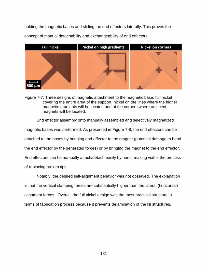
181

holding the magnetic bases and sliding the end effectors laterally. This proves the

concept of manual detachability and exchangeability of end effectors.

Figure 7-7: Three designs of magnetic attachment to the magnetic base: full nickel covering the entire area of the support, nickel on the lines where the higher magnetic gradients will be located and at the corners where adjacent magnets will be located.

End effector assembly onto manually assembled and selectively magnetized

magnetic bases was performed. As presented in Figure 7-8, the end effectors can be

attached to the bases by bringing end effector to the magnet (potential damage to bend

the end effector by the generated forces) or by bringing the magnet to the end effector.

End effectors can be manually attach/detach easily by hand, making viable the process

of replacing broken tips.

Notably, the desired self-alignment behavior was not observed. The explanation

is that the vertical clamping forces are substantially higher than the lateral (horizontal)

alignment forces. Overall, the full nickel design was the most practical structure in

terms of fabrication process because it prevents delamination of the Ni structures.

182

Figure 7-8: End effectors assembly tests. A) Attachment by bringing end effector to magnet or magnet to end effector. B) Attachment strength to manually assembled and selectively magnetized magnetic base. C) Replacement/detachability of broken end effector.

7.2.2 Supporting Tethers and Sacrificial Layer

Variations on the end effectors design were made to include tethers with notches

to support the structures during the releasing step. These variations were made when

introducing hybrid materials (SU-8 and nickel) for the second generation of end effector.

In this second generation of end effectors it was also evaluated a polymeric sacrificial

layer instead of the titanium. By using LOR (lift off resist) it was possible to reduce the

releasing time and enhance the fabrication yield. Figure 7-9 compares samples with

both sacrificial layers and the usage of the tethers before releasing. Thicknesses of

2 mm x 2 mm manually assembled magnetic base

3 mm x 3 mm selectively magnetized base

Nickel end effector

1st generation

Copper end effector

1st generation

2 mm x 2 mm manually assembled magnetic base

3 mm x 3 mm selectively magnetized base

Nickel end effector

1st generation

Copper end effector

1st generation

Broken end effector

End effector replacement

A

B

C

Bring end effector to magnet

Bring magnet to end effector

Remove debris Replace end effector

Attachment to manually assembled base

Attachment to selectively magnetized base

183

each material involved in the fabrication of the second generation of end effectors were

measured using profilometer (Tencor AS500) and presented in Table 7-2.

Figure 7-9: Examples of end effectors fabricated in the second generation. A) Using Ti and B) LOR as sacrificial layer. Unreleased structures.

Table 7-2. Thickness measurement of each material in the end effector.

Material Ti sacrificial layer LOR sacrificial layer

Nickel 13 µm 11 µm SU-8 6 µm 6 µm

SU-8 + Nickel 18 µm 16 µm Seed layer 243 nm 262 nm

7.2.3 End Effector Materials

Examples of fully fabricated end effectors in the four proposed techniques are

presented in Figure 7-10, with an example end effector array (before releasing)

demonstrating a batch microfabrication process. Cu and Ni successful resulted in rigid

structures that can protrude over 2 mm without bending with the weight of the beam

itself (as shown in Figure 7-2). However, end effector deformation (curling) was

observed in SU-8 structures during structure release. It is feasible to obtain successful

end effectors made of SU-8, but they may require much thicker structural layers.

Tethers

Ni

LOR Ni +SU-8

SU-8

100 µm

LOR sacrificial layer before releasing

B

Ni

Ti

Ti sacrificial layer before releasing

Tethers

A

100 µm

SU-8

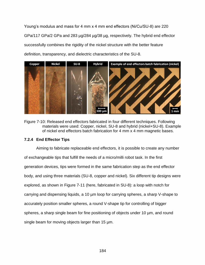
184

Young’s modulus and mass for 4 mm x 4 mm end effectors (Ni/Cu/SU-8) are 220

GPa/117 GPa/2 GPa and 283 µg/284 µg/38 µg, respectively. The hybrid end effector

successfully combines the rigidity of the nickel structure with the better feature

definition, transparency, and dielectric characteristics of the SU-8.

Figure 7-10: Released end effectors fabricated in four different techniques. Following materials were used: Copper, nickel, SU-8 and hybrid (nickel+SU-8). Example of nickel end effectors batch fabrication for 4 mm x 4 mm magnetic bases.

7.2.4 End Effector Tips

Aiming to fabricate replaceable end effectors, it is possible to create any number

of exchangeable tips that fulfill the needs of a micro/milli robot task. In the first

generation devices, tips were formed in the same fabrication step as the end effector

body, and using three materials (SU-8, copper and nickel). Six different tip designs were

explored, as shown in Figure 7-11 (here, fabricated in SU-8): a loop with notch for

carrying and dispensing liquids, a 10 µm loop for carrying spheres, a sharp V-shape to

accurately position smaller spheres, a round V-shape tip for controlling of bigger

spheres, a sharp single beam for fine positioning of objects under 10 µm, and round

single beam for moving objects larger than 15 µm.

185

Figure 7-11: Fabrication of different tools and resolutions (~10 µm) at the tip of the end effectors: Loop (with/without notch), V shape (sharp/round) and single beam (sharp and round).

Additional geometries were designed for the second generation of end effectors,

including liquid handling capabilities in a pen-like shape, a ~7 µm loop with a notch and

a fork to better manipulation of spherical objects. Examples of the designs fabricated in

nickel are presented in Figure 7-12. The smallest tip diameter obtained with nickel end

effectors was 4.7 µm.

Figure 7-12: Three examples of end effector tips made in nickel: A pen-like shape to dispense liquids, a loop with a notch to transport small spheres and a fork for positioning objects.

186

Successful hybrid end effectors were fabricated and released. Three

configurations of SU-8 and nickel were tested and represented in Figure 7-13: (1) Were

the SU-8 is totally contained inside the boundaries of nickel structure, forming 3D

structure (Out-plane circle). (2) The SU-8 has a conformable shape surrounding the

nickel structure (fork and sharp V-shape). (3) The active section of the tip is fabricated

in SU-8 and is protruding from the nickel (liquid handling and square). The minimum tip

diameter obtained in the SU-8 section of the hybrid tip was 3.8 µm. This result confirms

an improvement on feature size resolution between first and second generation of end

effectors.

Figure 7-13: Hybrid end effector tips made of nickel and SU-8. The SU-8 can be positioning in three configurations: Totally contained inside the nickel structure (Out of plane circle), conforming the nickel structure (fork and sharp V-shape) and with the active section protruding from the nickel (liquid handling and square).

7.3 End Effector Testing

First generation nickel end effectors were magnetically attached to magnetic

bases, creating a fully assembled levitated microrobot. End effector tips were dip-coated

187

in styrene-butadiene-styrene (SBS) following procedures in [247] to enhance adhesion

with objects to be manipulated. To facilitate the process, the SBS was dissolved in

toluene before dip coating. After coating the toluene is evaporated at room temperature.

Figure 7-14 illustrates the usage of the end effectors to manipulate a 10 µm gold wire A)

and a 1005-package surface mount technology (SMT) resistor (1 mm x 0.5 mm). For

demonstration purposes, the end effectors were mounted with the cooper seed layer

facing up in Figure 7-14A and the nickel facing up Figure 7-14B therefore the difference

in color. The functionality of the end effectors was unaltered when flipping the end

effectors.

Figure 7-14: Top view of nickel end effector mounted on magnetic bases and manipulating objects. A) Sharp single beam tip carrying 10 µm diameter gold wire. Seed layer facing up. B) Sharp V shape tip carrying a SMT resistor. Nickel facing up. Adhesion is enhanced by using SBS polymer (elastomer).

The assembled levitated microrobots with nickel end effectors were successfully

tested using the SRI microfactory platform, proving that there was no deleterious

electromagnetic interference between the driving platform and the end effectors, nor

interference with the levitation of the magnetic base. End effectors were successfully

used to manipulate a nickel square test piece (150 µm x 150 µm x 11 µm) and transport

it to a sticky surface as presented in Figure 7-15.

2 mm 2 mm

1.4 mm x 1.4 mm magnets on bot sticking out

Adhesive polymer coating

1 mm

Picked 1 x 0.5 mm SMT resistor

Limit of polymer coating

10 m diameter gold wireMagnetic

base

End effector

A B

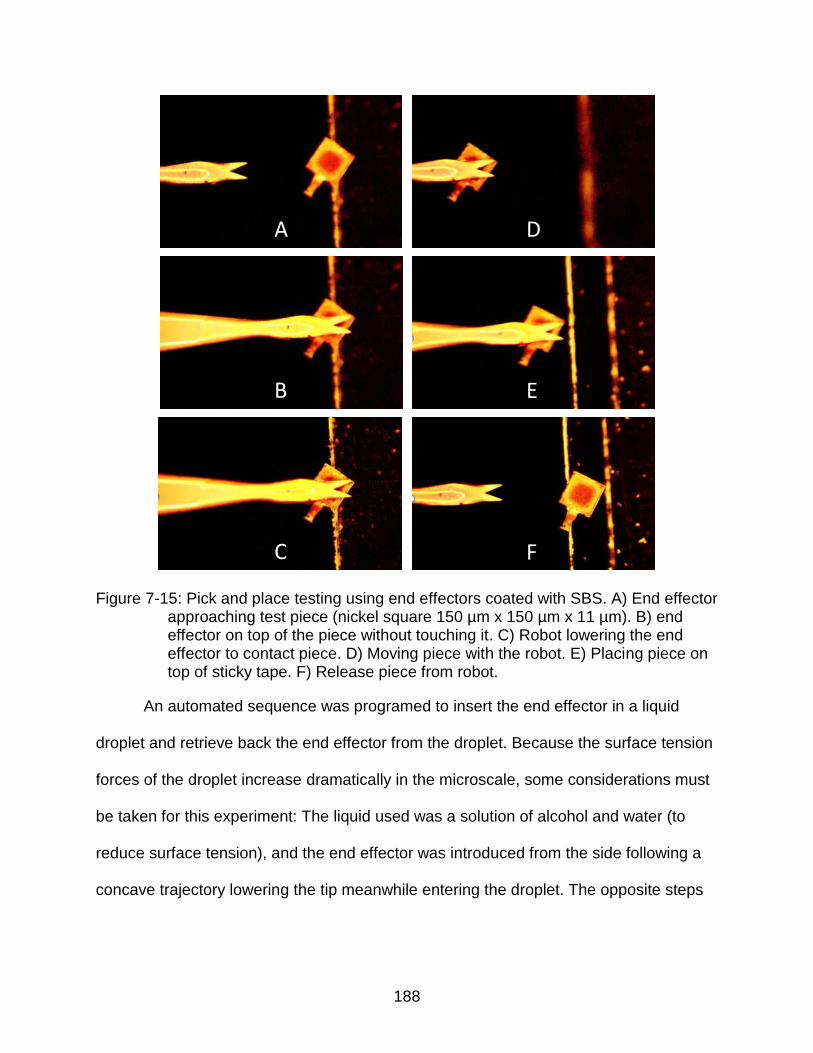
188

Figure 7-15: Pick and place testing using end effectors coated with SBS. A) End effector approaching test piece (nickel square 150 µm x 150 µm x 11 µm). B) end effector on top of the piece without touching it. C) Robot lowering the end effector to contact piece. D) Moving piece with the robot. E) Placing piece on top of sticky tape. F) Release piece from robot.

An automated sequence was programed to insert the end effector in a liquid

droplet and retrieve back the end effector from the droplet. Because the surface tension

forces of the droplet increase dramatically in the microscale, some considerations must

be taken for this experiment: The liquid used was a solution of alcohol and water (to

reduce surface tension), and the end effector was introduced from the side following a

concave trajectory lowering the tip meanwhile entering the droplet. The opposite steps

A

B

C

D

F

E

189

were followed to retrieve the end effector. Clips from a video demonstrating the

procedure were organized in a sequence presented in Figure 7-16.

Figure 7-16: Sequence of the end effector entering and leaving a droplet solution of alcohol and water (for reducing surface tension).

Another interesting application for the end effectors is the possibility to use them

for micro electro discharge machining (µEDM) [248], [249]. By connecting in series, the

electrically conducive end effectors (nickel or copper) to a high voltage circuit ended in a

conductive thin film layer (gold-coated polyamide tape), the circuit could only be closed

if the pointy tip of the end effector reach the film layer (Figure 7-17). Right before

touching the film, the end effector will discharge energy used to create an eroding spark

that will consume the gold layer. The precision, position and direction of the erosion are

dependent on the microrobot positioning and electrical circuit. µEDM is beyond the

scope of this dissertation. The experiment reported at Figure 7-17 was conducted as a

proof of concept at SRI laboratories but experiment conditions were not shared with

researches at University of Florida for confidentiality reasons.

190

Figure 7-17: Sequence demonstrating the proof of concept of micro electro discharge machining (µEDM) using nickel end effectors.

7.4 Summary

Herein we demonstrate successful batch fabrication of two generations of

detachable/exchangeable end effectors. The first generation made of Cu, Ni and SU-8

had thickness between 10-13 µm and minimum tip diameter of 4.7 µm. The second

hybrid generation is fabricated on Ni with SU-8 tips were 6 µm thick and minimum tip

diameter of 3.8 µm. The Cu and Ni end effectors prove more robust than the SU-8. Fully

assembled microrobots are achieved by attaching the end effectors to magnetic bases

Polyimide tape coted in gold

End effector

V

µEDM

Displacement of the robot

Gold removed

191

using nickel attachment structures embedded in the end effector bodies. This magnetic

attachment can withstand the weight of ~12 mg (magnetic base of 2x2 magnets) when

lifting the robot by the end effector. End effectors are entirely fabricated using standard

microfabrication techniques, therefore demonstrating the possibility of batch fabrication

of hundreds of interchangeable end effectors in the same lot. Eight different end effector

tips (tools) with micrometer scale features are successfully implemented, demonstrating

the potential of having multiple exchangeable tools designed for specific tasks.

The end effectors fully assembled on levitated microrobots proved to be useful

for manipulated objects at milli-scale (gold wire and SMT resistors), further tests must

be conducted to demonstrate manipulation of objects at the micro-scale. Fabricated

robots also proved to have a straightforward interaction with the microfactory platform

(no electromagnetic interference), and no interference with the levitation.

192

CHAPTER 8 ADDING FUNCTIONALITY TO MICROROBOTS: ELECTROPERMANENT MAGNETS*

Electropermanent magnets (EPM) can play an important role on microgrippers,

microrobot end-effectors, microfluidic systems, mechanobiology, MEMS and actuators.

This work describes the simulation, fabrication, and experimental demonstration of the

smallest reported EPM and subsequent simulation as an actuator for microgrippers.

Highly miniaturized EPMs— a NdFeB EPM (900 µm x 2000 µm x 500 µm) and a flexible

iron oxide EPM (790 µm x 1000 µm x 500 µm, one order of magnitude smaller than

state of the art)—are fabricated using precision dicing and microassembly of bulk

magnetic materials. The stray fields from the as-fabricated EPM devices are measured,

demonstrating a 15x ratio for the fields between the “on” and “off” states. Additionally,

theoretical and simulation models predict the function as actuation mechanism in

microgrippers.

A second section of this chapter will describe the fabrication of sub-millimeter

axisymmetric electropermanent magnets (EPMs), introducing for the first time a

fabrication technique for EPM that involves flexible magnets and bonded magnetic

powders. Two different bonded magnets were investigated: NdFeB and SmCo,

obtaining magnetic field on/off ratios of 2.8 and 4.6 respectively. Compared to magnet

assembly, the fabricated axisymmetric EPM provides: 1) symmetric magnetic field along

the magnetization axis, as opposed to the asymmetric fields in the transverse direction,

2) a path for future microfabrication, and 3) an alternative for mass production using roll-

to-roll process.

* This section contains excerpts from reference [250]. Special thanks to Catlin Beker, Zahira Gonzalez,

Lars Tatum and Dr. Johann Osma for their contribution on this chapter.

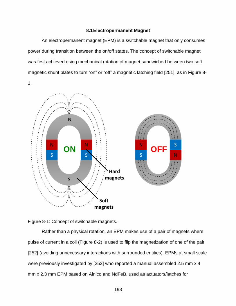
193

8.1 Electropermanent Magnet

An electropermanent magnet (EPM) is a switchable magnet that only consumes

power during transition between the on/off states. The concept of switchable magnet

was first achieved using mechanical rotation of magnet sandwiched between two soft

magnetic shunt plates to turn “on” or “off” a magnetic latching field [251], as in Figure 8-

1.

Figure 8-1: Concept of switchable magnets.

Rather than a physical rotation, an EPM makes use of a pair of magnets where

pulse of current in a coil (Figure 8-2) is used to flip the magnetization of one of the pair

[252] (avoiding unnecessary interactions with surrounded entities). EPMs at small scale

were previously investigated by [253] who reported a manual assembled 2.5 mm x 4

mm x 2.3 mm EPM based on Alnico and NdFeB, used as actuators/latches for

ON OFF

194

microrobots and programmable matter. Padovani et al. [254] presented a 3.2 mm x 4

mm x 3.6 mm EPM application for the control of a droplet inside a microfluidic system

and generated a magnetic field of 50 mT.

Figure 8-2: Concept of electropermanent magnet. The EPM will remain in the designated state in the absence of electrical currents.

There are multiple application drivers for miniaturization of this component such

as actuators/latches for microrobots and programmable matter [3], ferrofluid droplet

manipulations in microfluidic devices [4], and more. This work focus is the permanent

magnet array and explores a novel axisymmetric EPM fabrication technique that is

amenable to miniaturization, building on the design principles previously proposed by

the authors in [5].

ON OFF

195

8.2 Sub-millimeter Electropermanent Magnets for Microgripper

Microgrippers [243] have been used for precise manipulation and assembly of

microscale elements and the most common actuation mechanisms are electrostatic

[255], electro-thermal expansion[256], thermos-magnetically[257], piezoelectric [242],

[258] and magnetic [241], [259]. Magnetic actuation results very attractive for the ability

to generate high forces through remote actuation. A previously reported magnetically

actuated microgripper [260] used a permanent magnet on one side of the gripper and a

ferrite on the other side (reverting the ferrite to attract them). A pulsed external magnetic

field on the surrounding environment is required. This work proposes an alternative

actuation mechanism to build a microgripper by using a magnet that can be remotely

turned on/off.

This work explores the feasibility of employing an EPM as an on/off microgripper

as shown in Figure 8-3. By placing the EPM at the end of a cantilever (top jaw of the

gripper) and an iron foil in front (bottom jaw). When the EPM is switched “off”, there is

no magnetic force and the gripper is open; when the EPM is switched “on”, the

magnetic force between the EPM and iron foil will bend the cantilever and close the

jaws of the gripper.

196

Figure 8-3: EPM schematics. A)EPM configurations in the on/off states. Magnetization on Magnet 1 (left) is fixed and Magnet 2 (right) is switching magnetizations. B) Schematic representation of microgripper configuration using EPM and C) on/off actuation.

8.2.1 Experimental Results

EPM Fabrication

An order-of-magnitude size down-scaling of EPMs using semiconductor dicing

technology (ADT dicing saw) is proposed. Two magnetic materials (hard ferromagnets)

were machined: (1) NdFeB magnets 650 µm x 1000 µm x 500 µm (thick/width/depth),

with remanence of Br=1.16 T, and coercivity of Hci=899 kA/m (μ0Hci=1.13 T), and (2)

flexible iron oxide magnets 540 µm x 500 µm x 500 µm, with remanence of Br=180 mT,

and coercivity of Hci=125 kA/m (μ0Hci=0.16 T). Two iron foils (soft ferromagnets) were

machined, with 125 µm of thickness, covered the magnets to conduct the magnetic flux.

Two EPMs were successfully assembled with the two magnetic materials as

presented in the insets of Figure 8-4. Each EPM consist of two magnets of the same

size and material, in between two iron foils. The NdFeB EPM was 900 µm x 2000 µm x

500 µm, and the flexible iron oxide EPM was 790 µm x 1000 µm x 500 µm. EPMs were

manually assembled and the switching magnet was mechanically rotated to change

on/off states. This consideration was made as initial approach to constraint the problem

Magnet 1

Magnet 2Magnet 1

Magnet 2c

cc

c

Iron

Iron

OFF state

ON state

Lb

Wb

Hb

EPM

Iron

foil

Gap

distance

OFF state

ON state

Microgripper

Iron

Iron

OFF

(a) (b)A B C

197

analysis to the magnetostatic domain and to focus on the behavior of the magnetic

materials without considering external currents.

A test bench with computer interface platform was built using a commercial Hall

effect sensor (SSE49) to measure the magnetic flux density ( B

field) produced by the

EPM after fabrication. According to these measurements, calculations for using a

single-turn solenoid and a straight wire circuits were made to generate the necessary

field to electrically switch the state of the EPM.

Measurement of EPM magnetic fields

The measured magnetic fields for each EPM are shown in Figure 8-4 for on/off

states. As expected, the NdFeB EPM presented a larger magnetic flux density at the

surface during “on” state (2.7 mT) in comparison with the iron oxide EPM (0.75 mT). On

the other hand, the NdFeB EPM presented lower on/off ratio (9) than the flexible iron

oxide (15). It is strongly suspected that the “off” state magnetic field of the iron oxide

EPM is in the resolution limits of the measurement system therefore, future

measurements of the magnetic fields with higher resolution equipment are suggested.

198

Figure 8-4: Magnetic field measurements for EPM fabricated with two materials: NdFeB (900 µm x 2000 µm x 500 µm) and flexible iron oxide (790 µm x 1000 µm x 500 µm). Insets present pictures of both fabrications (depth for both pictures is 500 µm).

According to the measured fields, the necessary current to invert the

magnetization direction of the flexible iron oxide magnet, when using a single-turn

solenoid of 750 µm radius and a straight wire circuits were calculated (currents of 187 A

and 895 A respectively). Future work will be dedicated to evaluate the strategies to

generate such currents and to flip the magnetization direction of the magnets.

8.2.2 Simulation Results

Three sets of finite element model simulations were implemented using

COMSOL® Multiphysics. (1) A 2D magnetostatic simulation predicted the stray

magnetic field generated by the EPM at on/off states. (2) By placing an iron foil in front

of the magnet and change the separation, it is possible to estimate the total force

generated by the EPM at each state (on/off) as a function separation. (3) Knowing the

2.70 mT

0.75 mT0.30 mT

0.05 mT0

1

2

3

4

5

NdFeB Flexible Iron Oxide

Ma

gn

etic

fie

ld [

mT

] ON OFF

1000 µm

790 µm

900 µm

2000 µm

199

force generated by the magnet it is possible to simulate the gripper deflection towards

the iron foil.

Magnetic Field Simulation

Simulations of the stray magnetic B

field at on/off states for the strongest EPM

(NdFeB) are presented in Figure 8-5 Simulations include an iron foil in front of the EPM

and two independent configurations with different EPM-foil separations were evaluated:

1 mm and 0 mm separation. Figure 8-6A summarizes simulation results for the “on”

state of the EPM at multiple separations. The maximum force when the EPM is “on” and

separation is 1 mm (microgripper will change from open to close) is ~686 mN. When the

EPM is “on” and separation is 0 mm (microgripper is touching the surface) the magnetic

force is ~881 mN.

Figure 8-5: NdFeB 1500 µm x 2000 µm x 500 µm EPM magnetic field lines simulation for “on” and “off” states when the distance between the EPM and the iron foil is zero.

ON STATE OFF STATE

10-8

10-7

10-6

10-5

10-4

10-3

10-2

10-1

|B| [T]

-300

-200

-100

0

100

200

300

|My| [kA/m]

200

Figure 8-6: COMSOL simulation results for a NdFeB EPM (540 µm x 1000 µm x 500 µm) at “on” state: A) Magnetic force vs gap distance. B) Beam displacement vs applied magnetic force.

Microgripper Mechanical Simulation

The beam dimensions were chosen considering the size and weight of the EPM

and the desire deflection produced by the magnetic force at 1 mm of distance. Using the

force values simulated above, it is possible to simulate the mechanical response of

cantilever beam by applying different point force loads at the tip of the beam.

Considering the EPM dimensions, the beam height and thickness were

constrained to 800 µm and 300 µm respectively. Considering the possibility of having

symmetrical beams (jaws) in the microgripper and each one bending half the separation

gap, an analytical solution for bending the beam 500 µm was found. The beam length is

obtained by solving Equation 8-1, the maximum deflection equation ( max ).

IE

LF

Si

bEPM

3

3

max

8-1

where EPMF is the magnetic force made by the EPM at “on” state, bL is the length

of the beam, SiE is the Silicon young’s modulus and I is the moment of inertia (

0

0.2

0.4

0.6

0.8

1

0 0.5 1 1.5 2 2.5 3

Magn

etic

fo

rce

[N]

Gap distance [mm]

0

200

400

600

800

0 0.2 0.4 0.6 0.8 1

Bea

m d

efle

ctio

n [

µm

]

Applied force [N]

Expected

deflection

A B

Selected

gap

201

12/3

bb HWI ). An appropriate length of ~8.6 mm was calculated to meet the desire

requirements. Thus, the beams with those dimensions are expected to suffer a

deformation of 500 µm when a magnetic force of 674 mN is applied. Simulations

confirmed the beam deflection as shown in Figure 8-7. Additionally, beam deflection

simulations for all forces calculated under section III. A. (Magnetic field simulation) for

different EPM separations were made and presented in Figure 8-6B.

Figure 8-7: Simulation of the beam stress and deflection when the EPM is “on”.

The weight of the EPM was considered for the beam deformation analysis. The

weight of each iron foil was 22.62 mg and each NdFeB magnet was 2.79 mg, thus, the

total EPM mass was 50.84 mg equivalent to a weight force of ~499 µN, which is

negligible compared to the magnetic forces acting on the beam. The deflection of the

beam due to the weight of the EPM was simulated to be 0.37 µm and also confirmed by

calculations.

Maximum

displacement:

~ 506 µm

0 100 200 300 400 500

Von Mises stress [MN/m2]

Y Distance [mm]

Z D

ista

nce

[m

m]

202

8.3 Axisymmetric Sub-millimeter Electropermanent Magnet

A design and fabrication of sub-millimeter axisymmetric electropermanent

magnets (EPMs) will be presented in this section. Figure 8-8 shows the operation

principle of the traditional EPM, and compares the conventional (transversal field [252]–

[254]) vs. the new (axisymmetric field) architectures. The axisymmetric architecture

aims to generate stray B fields and latching forces along the axis, using two concentric

permanent magnets and two soft magnetic cap plates.

Figure 8-8: Operational concept of the conventional and new axisymmetric EPM architectures showing the ON and OFF states.

8.3.1 Simulations of the Axisymmetric EPM

Using 2D simulations in COMSOL Multiphysics, the B fields and latching forces

of both architectures are studied as a function of several design variables: outer radius,

permanent magnet aspect ratio and radius ratio, and cap plate thickness. For this

investigation, the following materials were assumed: grade N52 NdFeB as fixed inner

magnet, grade 5 Alnico for the outer switching magnet, and mild/low-carbon steel (AISI

1018) for the cap plates. The cap plate thickness was found to be an important variable

for tuning the on/off latching force ratio Figure 8-9 shows the final proposed dimensions

203

as a function of the magnetic layer thickness (T). These dimensions were selected to

maximize the on/off latching force ratio for a given cap plate thickness.

Figure 8-9: Example EPM configuration yielding maximum latching force on/off ratio

Simulations of the stray magnetic field of the optimal EPM evidence ~10x

difference in B field near the EPM poles in the on/off states (Figure 8-8A). Figure 8-8B

shows the magnitude of the on/off B-fields along the central axis with and without the

cap plates. Additional modeling is used to predict the latching force to a semi-infinite

steel plate. Figure 8-8C shows how the on/off latching force ratio can be tuned by

changing the thickness of the cap plates. Simulations of the new configuration

(dimensions used in Figure 8-9) suggest an on/off force ratio of 450, with the ability for

tuning this ratio from 1 up to 784, for sizes between 8 mm3 and 34 mm3, respectively.

These results suggest the new axisymmetric design may afford hundred-fold higher

latching force ratio than conventional EPM architectures in 1/10th the volume.

OFF configuration ON configuration

Co

nve

nti

on

al(T

ran

sver

sal)

New

(Axi

sym

met

ric)

(a) (b)

204

Figure 8-8: 2D axisymmetric COMSOL simulation. A) B field norm contour plots. B) Comparison of on/off fields for EPM with and without cap plates. C) Latching force generated by different EPM’s (on and off states) vs. thickness of the steel plates.

Simulations and optimization of sub-millimeter axisymmetric electropermanent

magnets (EPMs) predicting a latching force on/off ratio of 784 with total volume of 34

mm3. Compared to conventional architectures, the axisymmetric design provides: 1)

better performance in a smaller form factor, 2) symmetric magnetic field along the

magnetization axis, as opposed to the asymmetric fields in the transverse direction, 3) a

path for future microfabrication, and 4) large tunability of the magnetic field on/off ratio

(therefore the force) as a function of design variables (e.g. radii and thickness).

8.3.2 Fabrication of the Axisymmetric EPM

The concentric magnets on the EPM are fabricated by punching ~1 mm diameter

holes (using a cutting cannula) on flexible iron oxide (switching magnet) magnetic

substrate, previously demagnetized. Bonded magnets (fixed magnet) are fabricated on

these holes using permanent magnet powder as the magnetic material and

cyanoacrylate glue as bonding agent (applied on both sides), following technique

described in [261]. Finally, a ~2 mm cutting cannula is aligned to punch the outer ring.

The resulting assembly (called EPM core) is presented in Figure 8-11. Two different

bonded magnets were analyzed: NdFeB (6 µm) and Sm2Co17 (~15 µm). EPM cores are

1.E-01

1.E+00

1.E+01

1.E+02

1.E+03

1.E-03

1.E-02

1.E-01

1.E+00

1.E+01

1.E-01 1.E+00 1.E+01

on

/off

fo

rce

ra

tio

Forc

e (

N)

Steel Thickness [mm]

OnOffForce Ratio

101

100

10-1

10-2

10-3

10-1 100 101

103

102

101

100

10-1

Forc

e [

N]

On

/off

fo

rce

ra

tio

Steel thickness [mm]

CBA

205

magnetically characterized by using vibration sample magnetometer (VSM) and

magneto optical images (MOI). A pulse magnetizer is used to switch the EPM cores

from ON state (pulsing 7 T in the axial direction) to OFF state (by pulsing -700 mT for

SmCo or -440 mT for NdFeB EPMs). Mild/low-carbon steel (AISI 1018) plates are milled

and glued to the EPM core to finish the EPM.

Figure 8-11: Fabrication of the EPM core. A) Top view and B) cross section. C) Frontal view of the EPM including caps.

8.3.3 Characterization of the Axisymmetric EPM

A switchable 2.1 mm diameter and 0.8 mm thickness EPM was fabricated using

the proposed technique. Magnetic characterization of the EPM cores using VSM (Figure

8-12), showed that the SmCo EPM presented higher remanence (µ0Mr = 117 mT) and

lower intrinsic coercivity (Hci=210 kA/m) than the NdFeB EPM (75 mT and 252 kA/m).

Bonded magnet

Flexible magnet

2.1

mm

0.9

mm

Bonded Flexible

A

B

0.8

mm

2.1 mm

Bondedmagnet

Flexible magnet

2.8 mm

3.1

mm

Carbon Steel

C

206

Figure 8-12: Magnetization curve (VSM) of two EPM core configurations: with NdFeB and SmCo as bonded magnets.

MOI characterization (Figure 8-13) of the ON and OFF states demonstrate that it

exists a reversal magnetic field capable to switch the magnetization of only one of the

concentric magnets (flexible iron oxide) without switching the fix magnet (bonded

magnet). Cross section measurements of the B field suggest that the average ON/OFF

ration of the magnetic cores for the SmCo (27.3 mT/-6 mT) and NdFeB (23 mT/8.3 mT)

EPM cores are 4.6 and 2.8 respectively. These are fundamental advances in the small-

scale fabrication of EPMs and an important demonstration of the working principle for

the axisymmetric EPM design.

207

Figure 8-13: Stray magnetic field (MOI) for ON and OFF states of the EPM. A)Two configurations with different bonded magnets are measured: NdFeB and SmCo. B) Cross section measurement over the X axis.

Different reverse magnetic fields were applied to each sample of NdFeB and

SmCo EPM and MOI measures were made. A full magnetization of (7 T) was always

applied before the reversal field (Figure 8-14A). Post processing treatment from MOI

data was made to calculate the magnetic flux (in units of nWb). For this calculation, the

outer diameter of the EPM was manually selected for each image (constant diameter

through all images). The integral of the magnetic flux density field (through the selected

circular area) was used to define the magnetic flux. A plot of the magnetic flux as a

function of the reversal magnetic field for each sample is presented in Figure 8-14B.

This plot demonstrates that it exists a reversal magnetic field that cancel completely the

magnetic flux of the EMP. This is a prove of concept of the feasibility of obtaining an

“off” state from the EPM. This reversal magnetic field to turn the EPM off is 430 mT for

the NdFeB sample and 300 mT for the SmCo sample.

SmC

oN

dFe

B

-1.0 -0.5 0.0 0.5 1.0

X [mm]

Bz [mT]

50

0

-50

-1.0

-0.5

0.0

0.5

1.0

ON OFF

100

-100

Y [

mm

]

-80

-60

-40

-20

0

20

40

60

80

-1.0 -0.5 0.0 0.5 1.0

Bz

[mT]

X [mm]

SmCo-ONSmCo-OFFNdFeB-ONNdFeB-OFF

A B

208

Figure 8-14: EPM magnets after applying different reverse magnetic fields. SmCo and NdFeB samples were fully magnetizing before each test. Magnetic flux density calculated from MOI data. MOI of EPM magnets (inset).

Fully assembled EPMs with the caps were used to measure the magnetic flux in

the on and off state (by applying the reversal magnetic field found below). Carbon steel

plates proved to be a bad choice because their dimensions generate leakage magnetic

fields that interfere with the accuracy of the measurement. Instead, 150 µm thick film

made of steel, was used to create the plates. The film was laminated (top and bottom of

the magnet) before punching the EPM. This technique self-align the core of the EPM

with the plates and guaranty the same diameter. Figure 8-15 illustrates the result of the

magnetic flux measurements for the fully assembled EPM. The proof of concept of a

EPM that can be turned “on” and “off” was demonstrated and magnetic flux on/off ratio

of ~2 were achieved for both samples (NdFeB and SmCo).

Future efforts should be made to optimize the reversal field value for the fully

assembled EPM and to maximize the on/off ratio.

-100

-50

0

50

100

0 200 400 600 800 1,000

Ma

gne

tic

flu

x [n

Wb

]

µ0·H field [mT]

NdFeBSmCo

300 mT

430 mT

0.0·Hc 0.75·Hc 1.0·Hc 2.0·Hc 3.0·Hc

SmCo

NdFeB

Bz[mT]30

-30

-20

-10

0

20

10

209

Figure 8-15: MOI from the fully assembled EPMs (with ferromagnetic plates). Calculation of the on/off magnetic flux ratio.

8.4 Summary

This work demonstrates successful design of a microgripper based on EPM

actuation using NdFeB magnets to obtain higher magnetic field. It also demonstrates

the fabrication of the two smallest EPM reported to date, a NdFeB EPM (900 µm x 2000

µm x 500 µm) and a flexible iron oxide EPM (790 µm x 1000 µm x 500 µm. The

structure generates an estimate magnetic field on/off ratio of 9 and 15 respectively.

Future magnetic field measurements with higher resolution are required to confirm this

ratio. An application of the EPM as a microgripper is demonstrated using finite-element

model simulations. These promising results validate a future microfabrication path of

such microgrippers and enable the technology advance towards smaller scales.

A novel axisymmetric configuration of EPM was proposed. A fabrication

technique that enables the batch microfabrication of this components was also

demonstrated. Two fully assembled EPM (SmCo and NdFeb) with magnetic flux on/off

ratio of ~2 were achieved.

Sm

Co

Nd

Fe

B

-1.0 -0.5 0.0 0.5 1.0

X [mm]

-1.0

-0.5

0.0

0.5

1.0

ON OFF

Y [

mm

]

Bz[mT]

30

-30

-20

-10

0

20

10

ON OFF

ON/OFF

NdFeB 34 nWb -18 nWb 1.9

SmCo 40 nWb -20 nWb 2.0

Magnetic Flux

210

CHAPTER 9 CONCLUSIONS

The presented work advanced the field of microrobotics by developing of a

micro-magnetic field pattern fabrication process called selective magnetization. The

process imprinted pre-designed mili/micro-scale patterns on hard magnetic thick films.

This process was modeled via the finite-element method to solve the magneto-quasi-

static Maxwell equations using the measured nonlinear magnetic properties of the

materials (magnetization curves) and successfully validated using experimental

characterization with two techniques: magneto-optical imaging and a scanning hall

probe. The model predicted the general trends observed in the experimental results.

Using the selective magnetization process, two applications were demonstrated

in this work: 1) the magnetic assembly of nanoparticles (bottom-up) for the manufacture

of releasable magnetic microstructures and 2) the batch fabrication of diamagnetic

levitated microrobots (to-down). Selective magnetization proved to be fundamental

enhancing both sub-millimeter fabrication approaches: Bottom-up and top-down.

Solutions for two fundamental problems in the field were presented: 1) A

successful batch fabrication process of microrobots, to counteract the low throughput of

manually assembled robots. 2) The creation of exchangeable end effectors and

magnetic actuators, to counteract the lack of functionality.

9.1 Summary of Research Contributions

A selective magnetization process was successfully implemented, with the

versatility to create complex magnetic field patterns to be used in nano/micro

application. The technology core is the magnetization mask. Three different alternatives

to produce these masks were presented: 1) A microfabricated nickel mask, with 150 µm

211

feature size, successfully magnetizing magnetic recording media. 2) A low aspect ratio

(0.6), with 1mm feature size, fabricated using end mill machining and successfully

magnetizing flexible iron oxide and NdFeB magnets, and 3) a high aspect ratio (10),

with 1 mm feature size, laser machined that successfully magnetized NdFeB.

Using selective magnetization, a novel fabrication technique was demonstrated

to obtain free-floating magnetic microrobots by in situ crosslinking of magnetically

assembled nanoparticles. Microrobots with square and cross shape were obtained with

external dimensions of 175 µm and 150 µm, respectively, with boundary line

dimensions of 230 80 nm in height and 3.9 1 µm in width. The magnetic microrobots

were successfully released from the substrate retaining their shape in suspension

during manipulation with external magnetic fields.

Additionally, using selective magnetization, a process was successfully

implemented to fabricate 9 diamagnetically levitated microrobots per batch. The

millimeter-scale robots utilized a checkerboard magnetic pole pattern imprinted into a

400-m-thick NdFeB substrate. Fabricated microrobots were capable of assisted

levitation (external magnetic field bias) and operation in sliding mode (lateral movement

using microfactory platform).

A magnetic force sensing technique for force range of ±1000 µN with 50 nN

resolution and with a minimum step size of 50 µm was also demonstrated. Resulting

magnetic forces measured using this method were compared with the analytical solution

of the forces between two magnets (with one fixed and the other raster the surface).

Measurements and an analytical model present a good agreement. The results

212

demonstrate this technology could be a valuable contribution to close the technological

gap for microscale magnetic force sensing.

Next, magnetically detachable/replaceable end effector were developed. A

fabrication recipe for these end effectors was created and successfully standardized

(over 4” wafer) to produce structures with nickel body and SU-8 tip tools. End effectors

accomplished the manipulation of objects at microscale and were successfully used to

perform micro-electro discharge machining (µEDM) with the microrobots.

Finally, the usage of electropermanent magnets as actuators for microrobot was

successfully demonstrated, by designing an EPM-based microgripper. The two smallest

EPM reported to date in literature were fabricated: a NdFeB EPM (900 µm x 2000 µm x

500 µm) and a flexible iron oxide EPM (790 µm x 1000 µm x 500 µm). Furthermore, a

novel axisymmetric configuration of EPM was proposed (leading to the filing of a patent)

and a fabrication technique that enables the batch microfabrication of this components

was also demonstrated.

9.2 Future Work

There is always room for improvement in research. It was fortunate that most of

the individual efforts described in this dissertation successfully demonstrated a proof of

concept of the respective technology. However, each effort has the potential for follow-

on work (especially in the emerging, infant-stage field of microrobotics). For example, in

the case of electropermanent magnets, it was demonstrated that the configuration of

magnets in the axisymmetric EPM can be magnetized to turn on/off the external

magnetic flux. Despite that, a full microfabrication of the EPM should be pursued in

future research projects. Another example is the work conducted with the bottom-up

approach of fabricating releasable magnetic structures can be continued by exploring

213

biomedical applications for the technique. What if before releasing, the structures are

coated with some medicine and they are remotely manipulated after release (i.e. using

magnetic resonances images MRI), to be used as drug delivery mechanism into cells,

tumors or damaged tissue.

9.2.1 Selective Magnetization

From all the topics covered in this document (and because of its broad relevance

and applicability), the one requiring special discussion of future work is the selective

magnetization process. Future work towards enhancing the selective magnetization

process must address alternatives to increase the magnetic fields (therefore

diamagnetic force) produced by selectively magnetized bases and make them levitate.

The alternative hypothesis to solve the problem is: during the reversal magnetization,

the magnetic field experienced by the substrate under the unexposed areas (magnetic

mask) is so high (between 1 T and 1.5 T), that the material start to demagnetize and

loose magnetic field. This problem is observed either using pulse magnetizer or VSM.

An alternative solution is to reduce the magnetic field in the unexposed areas.

One way to do it is to follow developments by the company called Correlated Magnetics.

This company has produced devices called PolyMagnets (cm size selectively

magnetized NdFeB magnets). They use a fabrication procedure [181], were they induce

magnetic field on a single ferromagnetic tip by driving current trough a coil and

magnetizing an individual square (pixel like). By displacing the tip in x and y and

repeating the magnetization they will “imprint” any designated pattern.

An alternative could be to combine Correlated Magnetics’ approach the selective

magnetization propose in this dissertation. To fabricate a magnetization mask in the

form of a C-shape transformer (like the one proposed by Figure 9-1), with a 450 µm

214

gap. The rationale is that an electric current pulse will generate a concentrated

magnetic field only under the mask patterns, reducing the external magnetic field in the

areas without the presence of a magnetization mask, leading towards the selective

magnetization of the substrate.

Figure 9-1: Fabrication process for magnetization mask to enhance the contrast during magnetization.

A proof of concept of the proposed C-shape transformer with a coil (transformer

configuration with the magnet substrate to be magnetized placed in the air gap) was

simulated. This configuration will potentially increase the field underneath the mask but

keep almost 0 T field everywhere else. A cross section of the 3D COMSOL simulations

are presented in Figure 9-2. The current and number of wire loops was selected so the

field in the gap was ~1.5 T.

Gap for substrate: 450 µm

Coil

Gap for substrate: 450 µm

215

Figure 9-2: Cross section of a 3D simulation of the Bz field generated by a coil and the mask.

As a control simulation, a laminated C shape core with no pattern was also

simulated. Figure 9-3A compares the Bz fields observed at the air gap in: the control

simulation (coil and core), the mask under surrounding external field (external field) and

the coil, the core and the mask (coil and mask). The results showed that by using a coil,

the field outside the patterns can be dramatically reduced by ~750 mT, and therefore

the magnetic contrast can be enhanced. Figure 9-3B presents the minimum and

maximum fields obtained and the calculated contrast superimpose over the DC

demagnetization curve of substrate. These results are encouraging because the

contrast was immediately duplicated. Further investigation is required to find the right

conditions to maximize the magnetizations of the patterns.

Top view

Top view: Zoom in, mask Bz [T]

Distance [mm]

216

Figure 9-3: Bz field simulations for three configurations. A) A block of steel with no pattern is simulated as a baseline (coil and core) and the two magnetization techniques are compared. B) Max and min fields comparison over BJA DC demagnetization curve.

By observing Figure 9-3A a new concern arises: The separation between poles

in the mask during reversal could affect the contrast. Three peaks can be observed in

the figure, the ones at the sides observe a contrast of ~0.8 meanwhile the one in the

middle has a contrast of ~0.4. A minimum separation between features in the mask

could exist to maximize contrast. If this is true, a single reversal magnetization will not

be enough to solve the problem. Multiple masks with the minimum separation between

poles should be aligned and used at different times to magnetize the designated patter

and obtain levitation.

9.2.2 End Effectors

For future fabrications of end effectors, the authors suggest to make the following

modifications on the process: (1) Use LOR as a sacrificial layer, this will improve the

quality of the resulted structures and reduce fabrication time. (2) Use AZ 422 MIF for

dissolving the LOR sacrificial layer. Other commercial stripper or developers (such as

A B

217

AZ 312 mif or PG remover) might etch the copper seed layer or detach the SU-8 from

the nickel. (3) Eliminate Ti as a protective material in the seed layer (replace this step

by etching the copper oxide using a 1:10 solution of hydrochloric acid and water), this

will prevent the peeling of end effectors during electroplating. (4) Avoid using magnetic

attachment structures, it was proven that these structures will not generate a self-

alignment of the end effector and not having them will simplify the process. (5) Fabricate

the body of the end effectors in nickel. As show before, the nickel offered magnetic

adhesion to the robot bases and high stiffness to support objects. (6) Keep two

separated steps for end effectors and tips but fabricate the tips by electroplating nickel

or copper (depending on the application). This will improve the adhesion between end

effector and tip, increasing yield and making the tethers more robust. (7) Invert the order

of the layers. Electroplate the tips first (smaller feature size) and then electroplate the

end effector body (bigger feature size). This will guaranty that the surface of the tip (the

one in direct contact with manipulated objects) will be flatter and smother.

In a broader vision of future work on end effectors, it is relevant to remember that

their functionality is totally dependable on the applications. New applications will require

different tools, therefore is necessary to continue improving this technology to create

alternatives that are more customizable by the end user. An interesting direction of this

concept is making the body end effector with the planar fabrication technologies

presented here, but using micro-nano scale 3D printing (i.e. Nanoscribe technlogy) for

creating the final tips.

9.3 Final Conclusions

Microrobotics is a ~30 years old field that technologically is still in its infancy

stage. Many physical phenomenon at the micro/nano level are not fully understood and

218

technical/technological challenge remain unsolved. Even though there are many and

fantastic potential applications (mainly in industrial manufacturing, military and

bioengineering) they still need more momentum to be considered opportunities for the

industry or governments and invest full steam in their development. It is the time for the

research community to take advantage of this fertile soil, numerous questions to solve

and infinite opportunities to explore. Microrobotics is living now the prophesy of Richard

Feynman that drove the semiconductor industry, fortify the microsystems community

and exploit in the nanotechnology potential: There's Plenty of Room at the Bottom.

The research presented in this dissertation, advanced another step towards the

realization of the dreams associated with microrobotics providing clever engineering

solutions to tackle technological two challenges: the batch fabrication of microrobots

and their functionality. The vehicle to advance this step is name “selective

magnetization”, a technique so versatile that proved to be useful to fabricate structures

with the two existing approaches: bottom-up (assembly nanoparticles into free floating

microrobots) and top down (machining centimeter magnets into levitated microrobots).

The importance of this work relays in the link between academia and industry.

Any technology looking to impact industry in a certain stage, necessary requires

advances in batch fabrication and that was precisely the direction of this work.

Contributions made in this research can potentially be used by industry to fabricate and

test (with the magnetic force measuring technique) better and more functional magnetic

devices at nano and micro scale.

This research carries the hope that the fabricated microrobots themselves can be

used in two scenarios: the free floating magnetically responsive microstructures, can

219

potentially be used by researchers in biomedical applications for drug delivery or even

theranostic applications, where is required precise remote manipulation of cell-size-

structures. By the other hand, the levitated robots are very close to contribute

manufacturing and 3D positions of complex devices with sub-micron accuracy.

Detachable end effectors will be indispensable to give customization and versatility to

the final customer.

The other inspiring technology brought by this research is in the direction of

functionality. The presented proof of concept of the microfabricated electropermanent

magnet, could inspire the research community with the idea of “digital micro magnets”.

This component is an actuator that could enhance the microrobots by giving them

“smart” tools.

The author of this dissertation, firmly believes that the true potential of

microrobotics will come when the advances in electronics start bridge the gap between

the promises of the micro/nano world and functionality of the meter scale world. And

that is the reason this research contributed towards the functionally of the next

generation of microrobots. Ultimately, humanity will continue pushing the limits of the

small scale, and only connecting the dots between independent technologies (i.e. the

nano – micro gap) we will be able to deliver the promises and vision to create enhanced

human-size products starting from atoms.

220

REFERENCES

[1] J. Wilson, “Robotics: Technologies and global markets,” 2016.

[2] Robotics_Technology_Consortium, “A Roadmap for US Robotics, From Internet to Robotics,” 2016.

[3] N. Petrillo, “IBISWorld US - Industry, Company and Business Research Reports and Information,” 2015. [Online]. Available: http://clients1.ibisworld.com/reports/us/industry/default.aspx?entid=4074. [Accessed: 11-Jun-2017].

[4] A. Mcwilliams, “The Market for Minimally Invasive Medical Devices,” 2016.

[5] A. Kumar, “Medical robotics and computer assisted surgery: the global market,” 2017.

[6] National Science Foundation, “NSF Award Search: Advanced Search.,” 2017. [Online]. Available: https://www.nsf.gov/awardsearch/advancedSearch.jsp. [Accessed: 11-Jun-2017].

[7] T. Fukuda, F. Arai, and M. Nakajima, Micro-nanorobotic manipulation systems and their applications, vol. 9783642363. 2013.

[8] C. Velez, W. C. Patterson, and D. P. Arnold, “Simulation and experimental validation of a selective magnetization process for batch-patterning magnetic layers,” in Journal of Physics: Conference Series, 2015, vol. 660, pp. 3–7.

[9] C. Velez, I. Torres-Díaz, L. Maldonado-Camargo, C. Rinaldi, and D. P. Arnold, “Magnetic Assembly and Cross-Linking of Nanoparticles for Releasable Magnetic Microstructures / Supporting information,” ACS Nano, vol. 9, no. 10, pp. 10165–10172, 2015.

[10] R. Feynman, “Infinitesimal Machinery,” J. Microelectromechanical Syst., vol. 2, no. 1, pp. 4–14, 1993.

[11] R. P. Feynman, “There’s (still) plenty of room at the bottom,” Applied Thermal Engineering, vol. 61, no. 2, pp. 22–36, 1960.

[12] B. J. Nelson, I. K. Kaliakatsos, and J. J. Abbott, “Microrobots for Minimally Invasive Medicine,” Annu. Rev. Biomed. Eng., vol. 12, no. 1, pp. 55–85, 2010.

[13] M. Sitti, H. Ceylan, W. Hu, J. Giltinan, M. Turan, S. Yim, and E. Diller, “Biomedical Applications of Untethered Mobile Milli/Microrobots,” Proc. IEEE, vol. 103, no. 2, pp. 205–224, 2015.

[14] M. Probst, K. Vollmers, B. E. Kratochvil, and B. J. Nelson, “Design of an Advanced Microassembly System for the Automated Assembly of Bio-Microrobots,” Proc. 5th Int. Work. MicroFactories, IWMF 2006, pp. 1–6, 2006.

[15] R. D. D. Souza, S. Sharma, A. Jacob, and A. Al Hashimi, “Microrobotics : Trends And Technologies,” Am. J. Eng. Res., vol. 5, no. 5, pp. 32–39, 2016.

221

[16] J. Agnus, N. Chaillet, C. Clévy, S. Dembélé, M. Gauthier, Y. Haddab, G. Laurent, P. Lutz, N. Piat, K. Rabenorosoa, M. Rakotondrabe, and B. Tamadazte, “Robotic microassembly and micromanipulation at FEMTO-ST,” J. Micro-Bio Robot., vol. 8, no. 2, pp. 91–106, 2013.

[17] A. M. Flynn, “Gnat Robots (And How They Will Change Robotics),” 1987.

[18] W. S. N. Trimmer, “Microrobots and micromechanical systems,” Sensors and Actuators, vol. 19, no. 3, pp. 267–287, 1989.

[19] J. Fluitman, “Microsystems technology: objectives,” Sensors Actuators A Phys., vol. 56, no. 1–2, pp. 151–166, 1996.

[20] K. E. Petersen, “Silicon as a mechanical material,” Proc. IEEE, vol. 70, no. 5, pp.

420–457, 1982.

[21] R. S. Fearing, “Survey of sticking effects for micro parts handling,” Proc. 1995 IEEE/RSJ Int. Conf. Intell. Robot. Syst. Hum. Robot Interact. Coop. Robot., vol. 2, pp. 212–217, 1995.

[22] F. Arai, D. Ando, T. Fukuda, Y. Nonoda, and T. Oota, “Micro manipulation based on micro physics-strategy based on\nattractive force reduction and stress measurement,” Proc. 1995 IEEE/RSJ Int. Conf. Intell. Robot. Syst. Hum. Robot Interact. Coop. Robot., vol. 2, pp. 236–241, 1995.

[23] J. J. Abbott, Z. Nagy, F. Beyeler, and B. J. Nelson, “Robotics in the Small Part I,” IEEE Robot. Autom. Mag., vol. 14, no. September, pp. 111–121, Jun. 2007.

[24] L. Dong and B. J. Nelson, “Robotics in the Small Part II,” IEEE Robot. Autom. Mag., no. September, pp. 111–121, 2007.

[25] B. J. Nelson, L. Dong, and F. Arai, “Micro/Nanorobots,” in Springer Handbook of Robotics, B. Siciliano and O. Khatib, Eds. Berlin, Heidelberg: Springer Berlin Heidelberg, 2008, pp. 411–450.

[26] Y. Bellouard, Microrobotics : methods and applications. CRC Press, 2010.

[27] N. Chaillet and S. Regnier, Microrobotics for Micromanipulation. Hoboken, NJ, USA: John Wiley & Sons, Inc., 2013.

[28] M. Gauthier and S. Régnier, Robotic Microassembly. IEEE Press, 2011.

[29] M. Gauthier, N. Andreff, and E. Dombre, Intracorporeal Robotics. ISTE - Wiley, 2014.

[30] S. Fatikow and U. Rembold, Microsystem Technology and Microrobotics. Springer-Verlag Berlin Heidelberg GmbH, 1997.

[31] Y. Guo, Selected topics in micro/nano-robotics for biomedical applications. Springer, 2010.

[32] Y. Sun and X. Liu, Micro- and Nanomanipulation Tools. Wiley-VCH, 2015.

[33] S. Fatikow, Automated Nanohandling by Microrobots. Springer, 2007.

222

[34] D. Zhang, Advanced Mechatronics and MEMS Devices. Springer, 2013.

[35] A. Sulzmann, “Microrobotics : Components and Applications,” in Proceedings of the SPIE, 1996, vol. 2906.

[36] I. Paprotny and S. Bergbreiter, Small-Scale Robotics. Springer, 2013.

[37] E. Bruno, S. Oussama, K. Frans, E. B. Siciliano, O. Khatib, and F. Groen, Springer Tracts in Advanced Robotics Volume 21 Springer Tracts in Advanced Robotics, Volume 21., vol. 15. Springer, 2006.

[38] B. R. Donald, C. G. Levey, I. Paprotny, and D. Rus, “Simultaneous Control of Multiple MEMS Microrobots,” in Springer Tracts in Advanced Robotics: Algorithmic Foundations of Robotics VIII, Springer, 2001, pp. 69–84.

[39] J. Breguet, S. Johansson, W. Driesen, and U. Simu, “A review on actuation principles for few cubic millimeter sized mobile micro-robots,” 10th Int. Conf. New Actuators (Actuator 2006), pp. 374–381, 2006.

[40] T. Xu, J. Yu, X. Yan, H. Choi, and L. Zhang, “Magnetic actuation based motion control for microrobots: An overview,” Micromachines, vol. 6, no. 9, pp. 1346–1364, 2015.

[41] K. E. Peyer, S. Tottori, F. Qiu, L. Zhang, and B. J. Nelson, “Magnetic helical micromachines,” Chem. - A Eur. J., vol. 19, no. 1, pp. 28–38, 2013.

[42] M. Hassanalian and A. Abdelkefi, “Classifications, applications, and design challenges of drones: A review,” Prog. Aerosp. Sci., no. November 2016, 2017.

[43] H. Ceylan, J. Giltinan, K. Kozielski, and M. Sitti, “Mobile Microrobots for Bioengineering Applications,” Lab Chip, 2017.

[44] K. E. Peyer, L. Zhang, and B. J. Nelson, “Bio-inspired magnetic swimming microrobots for biomedical applications.,” Nanoscale, vol. 5, no. 4, pp. 1259–72, 2013.

[45] M. M. Stanton and S. Sánchez, “Pushing Bacterial Biohybrids to In Vivo Applications,” Trends Biotechnol., vol. xx, pp. 2–5, 2017.

[46] L. Zheng, L. guo Chen, H. bo Huang, X. peng Li, and L. lei Zhang, “An overview of magnetic micro-robot systems for biomedical applications,” Microsyst. Technol., vol. 22, no. 10, pp. 2371–2387, 2016.

[47] I. L. Sokolov, V. R. Cherkasov, A. A. Tregubov, S. R. Buiucli, and M. P. Nikitin, “Smart materials on the way to theranostic nanorobots: Molecular machines and nanomotors, advanced biosensors, and intelligent vehicles for drug delivery,” Biochim. Biophys. Acta - Gen. Subj., no. in-press, 2017.

[48] L. Dong, A. Subramanian, and B. J. Nelson, “Carbon nanotubes for nanorobotics,” Nano Today, vol. 2, no. 6, pp. 12–21, 2007.

[49] A. Dewan, S. U. Ay, M. N. Karim, and H. Beyenal, “Alternative power sources for remote sensors: A review,” Journal of Power Sources, vol. 245. 2014.

223

[50] J. G. S. Moo, C. C. Mayorga-Martinez, H. Wang, B. Khezri, W. Z. Teo, and M. Pumera, “Nano/Microrobots Meet Electrochemistry,” Adv. Funct. Mater., p. 1604759, 2017.

[51] M. Wehner, R. L. Truby, D. J. Fitzgerald, B. Mosadegh, G. M. Whitesides, J. A. Lewis, and R. J. Wood, “An integrated design and fabrication strategy for entirely soft, autonomous robots,” Nature, vol. 536, no. 7617, pp. 451–455, 2016.

[52] D. Rus and M. T. Tolley, “Design, fabrication and control of soft robots,” Nature, vol. 521, no. 7553, pp. 467–475, 2015.

[53] L. Hines, K. Petersen, G. Z. Lum, and M. Sitti, “Soft Actuators for Small‐ Scale Robotics,” Adv. Mater., 2016.

[54] E. P. Furlani, Permanent Magnet and Electromechanical Devices: Materials, Analysis, and Applications. Academic Press, 2001.

[55] E. Y. Tsymbal, “Section 6: Magnetostatics,” 2015.

[56] J. M. Camacho and V. Sosa, “Alternative method to calculate the magnetic field of permanent magnets with azimuthal symmetry,” Rev. Mex. Fis. E, vol. 59, no. 1, pp. 8–17, 2013.

[57] G. Xiao-fan, Y. Yong, and Z. Xiao-jing, “Analytic expression of magnetic field distribution of rectangular permanent magnets,” Appl. Math. Mech., vol. 25, no. 3, pp. 297–306, 2004.

[58] M. Getzlaff, Fundamentals of magnetism. Springer, 2008.

[59] a. Smith, K. K. Nielsen, D. V. Christensen, C. R. H. Bahl, R. Bjørk, and J. Hattel, “The demagnetizing field of a nonuniform rectangular prism,” J. Appl. Phys., vol. 107, pp. 1–8, 2010.

[60] A. Aharoni, “Demagnetizing factors for rectangular ferromagnetic prisms,” J. Appl. Phys., vol. 83, no. 6, p. 3432, 1998.

[61] A. Aharoni, “‘Local’ Demagnetization in a Rectangular Ferromagnetic Prism,” Phys. Status Solidi, vol. 229, no. 3, pp. 1413–1416, 2002.

[62] A. Aharoni, L. Pust, and M. Kief, “Comparing theoretical demagnetizing factors with the observed saturation process in rectangular shields,” J. Appl. Phys., vol. 87, no. 9, pp. 6564–6566, 2000.

[63] B. C. Dodrill, “Measurements with a VSM,” 2015.

[64] W. C. Patterson, “Of magnetic imaging system experiments and micro electro-mechanical systems ‘of mise and MEMS,’” Doctoral dissertation, University of Florida, 2015.

[65] W. C. Patterson, N. Garraud, E. E. Shorman, and D. P. Arnold, “A magneto-optical microscope for quantitative measurement of magnetic microstructures,” Rev. Sci. Instrum., vol. 86, no. 9, 2015.

224

[66] Camilo, Velez, Isaac, Torres-Díaz, Lorena, Maldonado-Camargo, Carlos, Rinaldi, D. P, and Arnold, “Magnetic Assembly and Cross-Linking of Nanoparticles for Releasable Magnetic Microstructures,” ACS Nano, vol. 9, no. 10, pp. 10165–10172, Oct. 2015.

[67] O. D. Oniku, A. Garraud, E. Shorman, W. C. Patterson, and D. P. Arnold, “Modeling of a Micromagnetic Imprinting Process,” in Tech. Dig. Solid-State Sensors, Actuators, and Microsystems Workshop (Hilton Head 2014), 2014, pp. 187–190.

[68] R. Bjørk, C. R. H. Bahl, a. Smith, and N. Pryds, “Comparison of adjustable permanent magnetic field sources,” J. Magn. Magn. Mater., vol. 322, no. 22, pp. 3664–3671, 2010.

[69] C. Velez, R. E. Carroll, and D. P. Arnold, “Direct measurement and microscale mapping of nanoNewton to milliNewton magnetic forces,” AIP Adv., vol. 7, no. 5, pp. 56809-1-56809–6, May 2017.

[70] S. Fahlbusch and S. Fatikow, “Force sensing in microrobotic systems-an overview,” 1998 IEEE Int. Conf. Electron. Circuits Syst. Surfing Waves Sci. Technol., vol. 3, pp. 259–262, 1998.

[71] Z. L. Z. Lu, P. C. Y. Chen, and W. L. W. Lin, “Force Sensing and Control in Micromanipulation,” IEEE Trans. Syst. Man Cybern. Part C Appl. Rev., vol. 36, no. 6, pp. 713–724, 2006.

[72] S. Alvo, P. Lambert, M. Gauthier, and S. Régnier, “A van der Waals Force-Based Adhesion Model for Micromanipulation,” J. Adhes. Sci. Technol., vol. 24, no. 15–16, pp. 2415–2428, 2010.

[73] C. Kian Ti, “Control of micromanipulation in the presence of van der Waals force,” National University of Singapore, 2003.

[74] M. Gauthier, N. Chaillet, S. Régnier, and P. Rougeot, “Analysis of forces for micromanipulations in dry and liquid media,” J. Micromechatronics, vol. 3, no. 3, pp. 389–413, 2006.

[75] K. Komvopoulos, “Surface engineering and microtribology for microeleetromechanical systems,” Wear, vol. 200, pp. 305–327, 1996.

[76] M. Hejazian, W. Li, and N.-T. Nguyen, “Lab on a chip for continuous-flow magnetic cell separation,” Lab Chip, vol. 15, no. 4, pp. 959–970, 2015.

[77] A. Garraud, C. Velez, Y. Shah, N. Garraud, B. Kozissnik, E. G. Yarmola, K. D. Allen, J. Dobson, and D. P. Arnold, “Investigation of the capture of magnetic particles from high-viscosity fluids using permanent magnets,” IEEE Trans. Biomed. Eng., vol. 63, no. 2, pp. 372–378, 2016.

[78] T. H. Boyer, “The force on a magnetic dipole,” Am. J. Phys., vol. 56, no. 8, pp. 688–692, 1988.

[79] L. Vaidman, “Torque and force on a magnetic dipole,” Am. J. Phys., vol. 58, no. 10, pp. 978–983, 1990.

225

[80] C. S. Siyambalapitiya, “Model and Validation of Static and Dynamic Behavior of Passive Diamagnetic Levitation for Energy Harvesting,” University of South Florida, 2012.

[81] J. J. Abbott, O. Ergeneman, M. P. Kummer, A. M. Hirt, and B. J. Nelson, “Modeling magnetic torque and force for controlled manipulation of soft-magnetic bodies,” IEEE Trans. Robot., vol. 23, no. 6, pp. 1247–1252, 2007.

[82] J.-P. Akoun, G.; Yonnet, “3D analytical calculation of the forces exerced between two cuboidal magnets,” Magn. IEEE Trans., vol. MAG-20, no. 5, pp. 1962–1964, 1984.

[83] J. S. Agashe and D. P. Arnold, “A study of scaling and geometry effects on the forces between cuboidal and cylindrical magnets using analytical force solutions,” J. Phys. D. Appl. Phys., vol. 42, pp. 099801–099801, 2009.

[84] H. Allag, J. P. Yonnet, and M. E. H. Latreche, “3D analytical calculation of forces between linear halbach-type permanent-magnet arrays,” 2009 8th Int. Symp. Adv. Electromechanical Motion Syst. Electr. Drives Jt. Symp. ELECTROMOTION 2009, no. July, pp. 1–3, 2009.

[85] W. Robertson, B. Cazzolato, and A. Zander, “Parameters for optimizing the forces between linear multipole magnet arrays,” IEEE Magn. Lett., vol. 1, 2010.

[86] W. Robertson, B. Cazzolato, and A. Zander, “A public framework for calculating the forces between magnets and multipole arrays of magnets,” Unpublished, pp. 1–6, 2010.

[87] D. C. Jiles, Introduction to Magnetism and Magnetic Materials, Second. Chapman & Hall/CRC, 1990.

[88] S. Earnshow, “On the Nature of the Molecular Forces which Regulate the Constitution of the Luminiferous Ether,” Transactions of the Cambridge, Philosophical Society, vol. 7. pp. 97–112, 1842.

[89] W. Braunbek, “Freischwebende Körper im elektrischen und magnetischen Feld,” Zeitschrift für Phys., vol. 112, no. 11–12, pp. 753–763, 1939.

[90] G. Kustler, “Diamagnetic levitation - Historical milestones,” Rev. Roum. Des Sci. Tech. Electrotech. Energ., vol. 52, no. 3, pp. 265–282, 2007.

[91] M. D. Simon and A. K. Geim, “Diamagnetic levitation: Flying frogs and floating magnets (invited),” J. Appl. Phys., vol. 87, no. 9, pp. 6200–6204, 2000.

[92] F. Barrot, “Acceleration and Inclination Sensors Based on Magnetic Levitation . Application in the Particular Case of Structural Health Monitoring in Civil Engineering,” École Polytechnique Fédérale de Lausanne, 2008.

[93] H. Bleuler, R. Moser, and J. Sandtner, “Diamagnetic suspension system for small rotors,” J. Micromechatronics, vol. 1, no. 2, pp. 131–137, Jan. 2001.

226

[94] H. Chetouani, B. Delinchant, and G. Reyne, “Efficient modeling approach for optimization of a system based on passive diamagnetic levitation as a platform for bio-medical applications,” COMPEL Int. J. Comput. Math. Electr. Electron. Eng., vol. 26, no. 2, pp. 345–355, 2007.

[95] F. Barrot, J. Sandtner, and H. Bleuler, “Acceleration Sensor Based on Diamagnetic Levitation,” IUTAM Symp. Vib. Control Nonlinear Mech. Struct., pp. 81–90, 2005.

[96] M. V Berry and A. K. Geim, “Of flying frogs and levitrons,” Eur. J. Phys., vol. 18, no. 4, pp. 307–313, 1997.

[97] R. D. Waldron, “Diamagnetic levitation using pyrolytic graphite,” Rev. Sci. Instrum., vol. 37, no. 1, pp. 29–35, 1966.

[98] H. D. Young and F. W. Sears, University physics. Extended version with modern physics. Addison-Wesley Pub. Co, 1992.

[99] G. Küstler, “Extraordinary levitation height in a weight compensated diamagnetic levitation system with permanent magnets,” IEEE Trans. Magn., vol. 48, no. 6, pp. 2044–2048, 2012.

[100] R. Moser, F. Barrot, J. Sandtner, and H. Bleuler, “Optimization of Two-Dimensional Permanent Magnet Arrays for Diamagnetic Levitation,” Int. Conf. Magn. Levitated Syst. Linear Drives, pp. 1–5, 2002.

[101] G. Küstler, “Diamagnetic levitation of pyrolytic graphite over monolithic NdFeB magnet,” Electron. Lett., vol. 50, no. 18, pp. 1289–1290, 2014.

[102] C. Emil, “Permanent Magnet Levitation Stabilized by Diamagnetic Materials: A case-study,” in Sixth International Conference on Computational Electromagnetics : CEM 2006, 2006, vol. 146, p. 633.

[103] M. Boukallel, J. Abadie, E. Piat, and A. Savary, “Levitated micro-nano force sensor using diamagnetic materials magnetic materials,” Proc. IEEE Int. Conf. Robot. Autom., pp. 3219–3224, 2003.

[104] D. B. Wilmink, “Theoretical and experimental investigations into magnetic levitation systems,” University of Adelaide, Australia, 2015.

[105] A. Minhaj, H. Fahad, H. Emdadul, O. Farrok, and M. Mynuddin, “Design and Construction of a Magnetic Levitation System Using Programmable Logic Controller,” Am. J. Mech. Eng., vol. 4, no. 3, p. 8, 2016.

[106] M. B. Khamesee, N. Kato, Y. Nomura, and T. Nakamura, “Design and control of a microrobotic system using magnetic levitation,” IEEE/ASME Trans. Mechatronics, vol. 7, no. 1, pp. 1–14, 2002.

[107] H. B. Profijt, C. Pigot, G. Reyne, R. M. Grechishkin, and O. Cugat, “Stable diamagnetic self-levitation of a micro-magnet by improvement of its magnetic gradients,” J. Magn. Magn. Mater., vol. 321, no. 4, pp. 259–262, 2009.

227

[108] E. Cazacu and I. Nemoianu, “Estimation of the influence terms involved in static diamagnetic levitation,” Rev. Roum. Des Sci. Tech. Electrotech. Energ., pp. 283–290, 2007.

[109] R. E. Pelrine, “Room temperature, open-loop levitation of microdevices using\ndiamagnetic materials,” IEEE Proc. Micro Electro Mech. Syst. An Investig. Micro Struct. Sensors, Actuators, Mach. Robot., pp. 1–4, 1990.

[110] R. Pelrine, A. Wong-Foy, B. McCoy, D. Holeman, R. Mahoney, G. Myers, J. Herson, and T. Low, “Diamagnetically levitated robots: An approach to massively parallel robotic systems with unusual motion properties,” Proc. - IEEE Int. Conf. Robot. Autom., pp. 739–744, 2012.

[111] H.-J. Butt, B. Cappella, and M. Kappl, “Force measurements with the atomic force microscope: Technique, interpretation and applications,” Surf. Sci. Rep., vol. 59, no. 1–6, pp. 1–152, 2005.

[112] F. A. Ferri, M. D. A. P. Da Silva, and E. M. Junior, “Magnetic Force Microscopy : Basic Principles and Applications,” At. Force Microsc. - Imaging, Meas. Manip. Surfaces At. Scale, 2012.

[113] T. Göddenhenrich, U. Hartmann, and C. Heiden, “Generation and imaging of domains with the magnetic force microscope,” Ultramicroscopy, vol. 42–44, no. PART 1, pp. 256–261, 1992.

[114] P. Grütter, D. Rugar, and H. J. Mamin, “Magnetic force microscopy of magnetic materials Sample,” Ultramicroscopy, vol. 47, pp. 393–399, 1992.

[115] U. Hartmann, “Magnetic force microscopy,” Russ. Chem. Rev., vol. 68, no. 3, pp. 165–170, 1999.

[116] U. Hartmann, T. Göddenhenrich, and C. Heiden, “Magnetic force microscopy: Current status and future trends,” J. Magn. Magn. Mater., vol. 101, no. 1–3, pp. 263–270, 1991.

[117] H. J. Hug, B. Stiefel, P. J. A. van Schendel, A. Moser, R. Hofer, S. Martin, H.-J. Güntherodt, S. Porthun, L. Abelmann, J. C. Lodder, G. Bochi, and R. C. OHandley, “Quantitative magnetic force microscopy on perpendicularly magnetized samples,” J. Appl. Phys., vol. 83, no. 11, pp. 5609–5620, 1998.

[118] M. R. Koblischka and U. Hartmann, “Recent advances in magnetic force microscopy,” Ultramicroscopy, vol. 97, no. 1–4, pp. 103–112, 2003.

[119] B. Moskowitz, “Magnetic Force Microscopy Techniques and Applications University of Minnesota,” in International Conference on Rock Magnetism and its Earth Science Applications, 2008.

[120] A. Schwarz and R. Wiesendanger, “Magnetic sensitive force microscopy,” Nano Today, vol. 3, no. 1–2, pp. 28–39, 2008.

228

[121] J. J. Sáenz, N. García, P. Grütter, E. Meyer, H. Heinzelmann, R. Wiesendanger, L. Rosenthaler, H. R. Hidber, and H. J. Güntherodt, “Observation of magnetic forces by the atomic force microscope,” J. Appl. Phys., vol. 62, no. 10, pp. 4293–4295, 1987.

[122] J. A. Sidles, J. L. Garbini, K. J. Bruland, D. Rugar, O. Zger, S. Hoen, and C. S. Yannoni, “Magnetic resonance force microscopy,” Rev. Mod. Phys., vol. 67, no. 1, pp. 249–265, 1995.

[123] Y. Martin and H. K. Wickramasinghe, “Magnetic imaging by ‘force microscopy’ with 1000 ?? resolution,” Appl. Phys. Lett., vol. 50, no. 20, pp. 1455–1457, 1987.

[124] Q. Liang, D. Zhang, G. Coppola, Y. Wang, S. Wei, and Y. Ge, “Multi-dimensional MEMS/micro sensor for force and moment sensing: A review,” IEEE Sens. J., vol.

14, no. 8, pp. 2643–2657, 2014.

[125] Y. Wei and Q. Xu, “An overview of micro-force sensing techniques,” Sensors Actuators, A Phys., vol. 234, pp. 359–374, 2015.

[126] R. J. J. J. Wood and R. S. S. S. Fearing, “Flight Force Measurements for a Micromechanical Flying Insect,” Proc. 2001 IEEE/RSJ Int. Conf. Intell. Robot. Syst. Expand. Soc. Role Robot. Next Millenn. (Cat. No.01CH37180), pp. 355–362, 2001.

[127] D. J. Cappelleri, G. Krishnan, C. Kim, V. Kumar, and S. Kota, “Toward the Design of a Decoupled, Two-Dimensional, Vision-Based μN Force Sensor,” J. Mech. Robot., vol. 2, no. 2, p. 21010, 2010.

[128] D. J. Cappelleri, G. Piazza, and V. Kumar, “Two-dimensional, vision-based µN force sensor for microrobotics,” {IEEE} Int. Conf. Robot. Autom., pp. 1016–1021, 2009.

[129] Y. H. Anis, J. K. Mills, and W. L. Cleghorn, “Vision-based measurement of microassembly forces,” J. Micromechanics Microengineering, vol. 16, no. 8, pp. 1639–1652, 2006.

[130] S. Muntwyler, F. Beyeler, and B. J. Nelson, “Three-axis micro-force sensor with tunable force range and sub-micronewton measurement uncertainty,” Proc. - IEEE Int. Conf. Robot. Autom., pp. 3165–3170, 2010.

[131] F. Beyeler, S. Muntwyler, and B. J. Nelson, “A Six-Axis MEMS Force – Torque Sensor With Micro-Newton and Nano-newtonmeter Resolution,” J. Microelectromechanical Syst., vol. 18, no. 2, pp. 433–441, 2009.

[132] P. Ripka and M. Janosek, “Advances in Magnetic Field Sensors,” IEEE Sens. J., vol. 10, no. 6, pp. 1108–1116, 2010.

[133] W. C. Patterson, N. Garraud, E. E. Shorman, and D. P. Arnold, “A magneto-optical microscope for quantitative measurement of magnetic microstructures,” Rev. Sci. Instrum., vol. 86, no. 9, pp. 1–10, 2015.

229

[134] L. Wang, M. Dkhil, A. Bolopion, P. Rougeot, S. Régnier, and M. Gauthier, “Simulation and Experiments on Magnetic MicroForces for Magnetic MicroRobots Applications,” in International Conference on Manipulation, Manufacturing and Measurement on the Nanoscale (3M-NANO), 2013, no. 26–30 August, pp. 15–20.

[135] G. Hwang, I. A. Ivan, J. Agnus, H. Salmon, S. Alvo, N. Chaillet, S. Régnier, and A. M. Haghiri-Gosnet, “Mobile microrobotic manipulator in microfluidics,” Sensors Actuators, A Phys., vol. 215, pp. 56–64, 2014.

[136] O. D. Oniku, B. Qi, and D. P. Arnold, “Electroplated thick-film cobalt platinum permanent magnets,” J. Magn. Magn. Mater., 2016.

[137] C. Velez, W. C. Patterson, and D. P. Arnold, “Simulation and experimental validation of a selective magnetization process for batch-patterning magnetic layers,” J. Phys. Conf. Ser., vol. 660, pp. 3–7, 2015.

[138] N. M. Dempsey, “Hard Magnetic Materials for MEMS Applications,” in Nanoscale Magnetic Materials and Applications, 2009, pp. 661–680.

[139] T. M. Liakopoulos, W. Zhang, and C. H. Ahn, “Micromachined Thick Permanent Magnet Arrays on Silicon Wafers,” IEEE Trans. Magn., vol. 32, no. 5, pp. 5154–5156, 1996.

[140] H. Guckel, K. J. Skrobis, T. R. Christenson, J. Klein, S. Han, B. Choi, E. G. Lovell, and T. W. Chapman, “Fabrication and testing of the planar magnetic micromotor,” J. Micromechanics Microengineering, vol. 1, no. 3, pp. 135–138, 1991.

[141] C. H. Ahn, Y. J. Kim, and M. G. Allen, “Planar variable reluctance magnetic micromotor with fully integrated stator and coils,” J. Microelectromechanical Syst., vol. 2, no. 4, pp. 165–173, 1993.

[142] B. Wagner, M. Kreutzer, and W. Benecke, “Linear and rotational magnetic micromotors fabricated using silicon technology,” in Proceedings IEEE Micro Electro Mechanical Systems, 1992, pp. 183–189.

[143] D. P. Arnold, N. Wang, and S. Member, “Permanent Magnets for MEMS,” J. Micromechanical Syst., vol. 18, no. 6, pp. 1255–1266, 2009.

[144] D. P. Arnold, “Review of microscale magnetic power generation,” IEEE Trans. Magn., vol. 43, no. 11, pp. 3940–3951, 2007.

[145] R. L. Harne and K. W. Wang, “A review of the recent research on vibration energy harvesting via bistable systems,” Smart Mater. Struct., vol. 22, no. 2, p. 23001, 2013.

[146] A. Amar, A. Kouki, and H. Cao, “Power Approaches for Implantable Medical Devices,” Sensors, vol. 15, no. 11, pp. 28889–28914, 2015.

[147] E. Romero, R. O. Warrington, and M. R. Neuman, “Energy scavenging sources for biomedical sensors,” Physiol. Meas., vol. 30, no. 9, pp. R35–R62, 2009.

[148] E. Romero, Powering Biomedical Devices. Academic Press, 2013.

230

[149] K. Halbach, “Design of permanent multipole magnets with oriented rare earth cobalt material,” Nucl Instrum Methods, vol. 169, no. 3, pp. 1–10, 1980.

[150] K. Yamaguchi, T. Fujita, Y. Tanaka, N. Takehira, K. Sonoda, K. Kanda, and K. Maenaka, “MEMS Batch Fabrication of the Bipolar Micro Magnet Array for Electromagnetic Vibration Harvester,” J. Phys. Conf. Ser., vol. 557, p. 12033, 2014.

[151] F. Herrault, B. C. Yen, C. Ji, Z. S. Spakovszky, J. H. Lang, and M. G. Allen, “Fabrication and Performance of Silicon-Embedded,” J. Micromechanical Syst., vol. 19, no. 1, pp. 4–13, 2010.

[152] B. a Peterson, W. C. Patterson, F. Herrault, D. P. Arnold, and M. G. Allen, “Laser-Micromachined Permanent Magnet Arrays With Spatially Alternating Magnetic Field Distribution,” in PowerMEMS, 2012, pp. 2–5.

[153] P. Chen, Y.-Y. Huang, G. Bhave, K. Hoshino, and X. Zhang, “Inkjet-Print Micromagnet Array on Glass Slides for Immunomagnetic Enrichment of Circulating Tumor Cells,” Ann. Biomed. Eng., 2015.

[154] S. Merzaghi, C. Koechli, and Y. Perriard, “Development of a hybrid MEMS BLDC micromotor,” IEEE Trans. Ind. Appl., vol. 47, no. 1, pp. 3–11, 2011.

[155] C. D. Riley, G. W. Jewell, and D. Howe, “The design and analysis of axial field multipole impulse magnetizing fixtures,” J. Appl. Phys., vol. 83, no. 1998, pp. 7112–7114, 1998.

[156] J. Töpfer, B. Pawlowski, H. Beer, K. Plötner, P. Hofmann, and J. Herrfurth, “Multi-pole magnetization of NdFeB magnets for magnetic micro-actuators and its characterization with a magnetic field mapping device,” J. Magn. Magn. Mater., vol. 270, pp. 124–129, 2004.

[157] J. B. Tracy and T. M. Crawford, “Magnetic field-directed self-assembly of magnetic nanoparticles,” MRS Bull., vol. 38, no. 11, pp. 915–920, Nov. 2013.

[158] P. A. Gilles, J. Delamare, and O. Cugat, “Rotor for a brushless micromotor,” J. Magn. Magn. Mater., vol. 242–245, no. PART II, pp. 1186–1189, 2002.

[159] H. Raisigel, O. Cugat, and J. Delamare, “Permanent magnet planar micro-generators,” Sensors Actuators A Phys., vol. 130–131, pp. 438–444, 2006.

[160] F. M. F. Rhen, E. Backen, and J. M. D. Coey, “Thick-film permanent magnets by membrane electrodeposition,” J. Appl. Phys., vol. 97, no. 11, p. 113908, 2005.

[161] F. Dumas-Bouchiat, L. F. Zanini, M. Kustov, N. M. Dempsey, R. Grechishkin, K. Hasselbach, J. C. Orlianges, C. Champeaux, A. Catherinot, and D. Givord, “Thermomagnetically patterned micromagnets,” Appl. Phys. Lett., vol. 96, no. 10, pp. 3–6, 2010.

231

[162] M. Kustov, P. Laczkowski, D. Hykel, K. Hasselbach, F. Dumas-Bouchiat, D. O’Brien, P. Kauffmann, R. Grechishkin, D. Givord, G. Reyne, O. Cugat, and N. M. Dempsey, “Magnetic characterization of micropatterned Nd–Fe–B hard magnetic films using scanning Hall probe microscopy,” J. Appl. Phys., vol. 108, no. 6, p. 63914, 2010.

[163] O. Osman, S. Toru, F. Dumas-Bouchiat, N. M. Dempsey, N. Haddour, L.-F. Zanini, F. Buret, G. Reyne, and M. Frenea-Robin, “Microfluidic immunomagnetic cell separation using integrated permanent micromagnets,” Biomicrofluidics, vol. 7, no. 5, p. 54115, 2013.

[164] N. M. Dempsey, D. Roy, H. Marelli-Mathevon, G. Shaw, a. Dias, R. B. G. Kramer, V. Cuong, M. Kustov, L. F. Zanini, C. Villard, K. Hasselbach, C. Tomba, F. Dumas-Bouchiat, D. Le Roy, H. Marelli-Mathevon, G. Shaw, a. Dias, R. B. G. Kramer, L. Viet Cuong, M. Kustov, L. F. Zanini, C. Villard, K. Hasselbach, C. Tomba, and F. Dumas-Bouchiat, “Micro-magnetic imprinting of high field gradient magnetic flux sources,” Appl. Phys., vol. 104, no. 26, p. 262401, 2014.

[165] L. F. Zanini, N. M. Dempsey, D. Givord, G. Reyne, and F. Dumas-Bouchiat, “Autonomous micro-magnet based systems for highly efficient magnetic separation,” Appl. Phys. Lett., vol. 99, no. 23, p. 232504, 2011.

[166] L. F. Zanini, O. Osman, M. Frenea-Robin, N. Haddour, N. M. Dempsey, G. Reyne, and F. Dumas-Bouchiat, “Micromagnet structures for magnetic positioning and alignment,” J. Appl. Phys., vol. 111, no. 7, p. 07B312, 2012.

[167] J. Pivetal, D. Royet, G. Ciuta, M. Frenea-Robin, N. Haddour, N. M. Dempsey, F. Dumas-Bouchiat, and P. Simonet, “Micro-magnet arrays for specific single bacterial cell positioning,” 10th Int. Conf. Sci. Clin. Appl. Magn. Carriers 10-14 June, 2014, Dresden, Ger., vol. 380, no. 0, pp. 72–77, 2015.

[168] R. Fujiwara, T. Shinshi, and E. Kazawa, “Micromagnetization patterning of sputtered NdFeB/Ta multilayered films utilizing laser assisted heating,” Sensors Actuators A Phys., vol. 220, pp. 298–304, 2014.

[169] J. Fassbender and J. McCord, “Magnetic patterning by means of ion irradiation and implantation,” J. Magn. Magn. Mater., vol. 320, no. 3–4, pp. 579–596, 2008.

[170] E. Menéndez, M. O. Liedke, J. Fassbender, T. Gemming, A. Weber, L. J. Heyderman, K. V. Rao, S. C. Deevi, S. Suriñach, M. D. Baró, J. Sort, and J. Nogués, “Direct Magnetic Patterning due to the Generation of Ferromagnetism by Selective Ion Irradiation of Paramagnetic FeAl Alloys,” Small, vol. 5, no. 2, pp. 229–234, 2008.

[171] D. G. Merkel, L. Bottyán, F. Tanczik, Z. Zolnai, N. Nagy, G. Vértesy, J. Waizinger, and L. Bommer, “Magnetic patterning perpendicular anisotropy FePd alloy films by masked ion irradiation,” J. Appl. Phys., vol. 109, no. 12, pp. 1–7, 2011.

[172] B. D. Terris, D. Weller, L. Folks, J. E. E. Baglin, a. J. Kellock, H. Rothuizen, and P. Vettiger, “Patterning magnetic films by ion beam irradiation,” J. Appl. Phys., vol. 87, no. 9, p. 7004, 2000.

232

[173] C. Vieu, J. Gierak, H. Launois, T. Aign, P. Meyer, J. P. Jamet, J. Ferre, C. Chappert, V. Mathet, and H. Bernas, “High resolution magnetic patterning using focused ion beam irradiation,” J. Chem. Inf. Model., vol. 53, pp. 1689–1699, 2013.

[174] Y. G. Wang and Y. Z. Huang, “Magnetic Patterning of Co/Pt Multilayers by Ga+ Ion Irradiation,” J. Electron. Mater., vol. 38, no. 3, pp. 468–474, 2008.

[175] D. P. Arnold, S. Das, J. Park, I. Zana, J. H. Lang, and M. G. Allen, “Microfabricated High-Speed Axial-Flux Multiwatt Permanent-Magnet Generators—Part II: Design, Design , Fabrication , and Testing,” Ieee Trans. Microelectromechanical Syst., vol. 15, no. 5, pp. 1351–1363, 2006.

[176] I. Zana, F. Herrault, D. Arnold, and M. Allen, “Magnetic patterning of permanent-magnet rotors for microscale motor/generators,” in Tech. Dig. 5th Int. Workshop on Micro and Nanotechnology for Power Generation and Energy Conversion Apps. PowerMEMS 2005, 2005, no. 404, pp. 0–3.

[177] O. Oniku, R. Regojo, Z. Kaufman, W. C. Patterson, and D. P. Arnold, “Batch Patterning of SubMillimeter Features in Hard Magnetic Films Using Pulsed Magnetic Fields and Soft Magnetizing Heads,” IEEE Trans. Magn., vol. 49, no. 7, pp. 4116–4119, Jul. 2013.

[178] B. a. Peterson, O. D. Oniku, W. C. Patterson, D. Le Roy, a. Garraud, F. Herrault, N. M. Dempsey, D. P. Arnold, and M. G. Allen, “Technology Development for Short-period Magnetic Undulators,” Phys. Procedia, vol. 52, pp. 36–45, 2014.

[179] O. D. Oniku, P. V. Ryiz, A. Garraud, and D. P. Arnold, “Imprinting of fine-scale magnetic patterns in electroplated hard magnetic films using magnetic foil masks,” J. Appl. Phys., vol. 115, no. 17, p. 17A718, 2014.

[180] A. Garraud, O. D. Oniku, W. C. Patterson, E. Shorman, D. Le Roy, N. M. Dempsey, and D. P. Arnold, “Microscale magnetic patterning of hard magnetic films using microfabricated magnetizing masks,” in 2014 IEEE 27th International Conference on Micro Electro Mechanical Systems (MEMS), 2014, pp. 520–523.

[181] M. D. Roberts, L. W. Fullerton, D. P. Machado, D. Mize, and K. Loum, “Magnetic structure production,” US 8648681 B2, 2014.

[182] O. D. Oniku, A. Garraud, E. E. Shorman, W. C. Patterson, and D. P. Arnold, “Modeling of a micromagnetic imprinting process,” in Tech. Dig. Solid-State Sensors, Actuators, and Microsystems Workshop (Hilton Head 2014), 2014, pp.

187–190.

[183] A. Garraud, O. D. Oniku, W. C. Patterson, E. Shorman, D. Le Roy, N. M. Dempsey, and D. P. Arnold, “Microscale magnetic patterning of hard magnetic films using microfabricated magnetizing masks,” in MEMS 2014, 2014, pp. 520–523.

[184] O. D. Oniku, P. V. Ryiz, A. Garraud, and D. P. Arnold, “Imprinting of fine-scale magnetic patterns in electroplated hard magnetic films using magnetic foil masks,” J. Appl. Phys., vol. 115, no. 17, p. 17A718, May 2014.

233

[185] E. O. Samwel, P. R. Bissell, and J. C. Lodder, “Remanent magnetic measurements on perpendicular recording materials with compensation for demagnetizing fields,” J. Appl. Phys., vol. 73, no. 3, pp. 1353–1359, 1993.

[186] E. Peli, “Contrast in complex images.,” J. Opt. Soc. Am. A., vol. 7, no. 10, pp. 2032–2040, 1990.

[187] Q. Dai and A. Nelson, “Magnetically-responsive self assembled composites.,” Chem. Soc. Rev., vol. 39, no. 11, pp. 4057–66, Nov. 2010.

[188] A. N. Shipway, E. Katz, and I. Willner, “Nanoparticle Arrays on Surfaces for Electronic , Optical , and Sensor Applications,” ChemPhysChem, vol. 1, pp. 18–52, 2000.

[189] M. Chirita and I. Grozescu, “Fe 2 O 3 – Nanoparticles , Physical Properties and Their Photochemical And Photoelectrochemical Applications,” Chem Bull Politeh. Univ Timsisoara, vol. 54, no. 68, pp. 1–8, 2009.

[190] G. K. Kouassi and J. Irudayaraj, “Magnetic and Gold-Coated Magnetic Nanoparticles As a DNA Sensor Magnetic and Gold-Coated Magnetic Nanoparticles As a DNA Sensor,” Society, vol. 78, no. 10, pp. 3234–3241, 2006.

[191] S. Qu, J. Wang, J. Kong, P. Yang, and G. Chen, “Magnetic loading of carbon nanotube/nano-Fe3O4 composite for electrochemical sensing,” Talanta, vol. 71, no. 3, pp. 1096–1102, 2007.

[192] J. L. Gong, Y. Liang, Y. Huang, J. W. Chen, J. H. Jiang, G. L. Shen, and R. Q. Yu, “Ag/SiO2 core-shell nanoparticle-based surface-enhanced Raman probes for immunoassay of cancer marker using silica-coated magnetic nanoparticles As separation tools,” Biosens. Bioelectron., vol. 22, no. 7, pp. 1501–1507, 2007.

[193] J. Wang, A. Munir, Z. Zhu, and H. S. Zhou, “Magnetic Nanoparticle Enhanced Suface Plasmon Resonance Sensing and Its Application for the Ultrasensitive Detection of Magnetic Nanoparticle-Enriched Small Molecules,” Anal. Chem., vol. 82, no. 16, pp. 6782–6789, 2010.

[194] J. Kim, S. E. Chung, S.-E. Choi, H. Lee, J. Kim, and S. Kwon, “Programming magnetic anisotropy in polymeric microactuators.,” Nat. Mater., vol. 10, no. 10, pp. 747–52, Oct. 2011.

[195] D. F. Emerich and C. G. Thanos, “The pinpoint promise of nanoparticle-based drug delivery and molecular diagnosis.,” Biomol. Eng., vol. 23, no. 4, pp. 171–84, Sep. 2006.

[196] A. Yethiraj, J. H. J. Thijssen, A. Wouterse, and A. Van Blaaderen, “Large-Area Electric-Field-Induced Colloidal Single Crystals for Photonic Applications,” Adv. Mater., vol. 16, no. 7, pp. 596–600, 2004.

[197] L. He, Y. Hu, H. Kim, J. Ge, S. Kwon, and Y. Yin, “Magnetic assembly of nonmagnetic particles into photonic crystal structures.,” Nano Lett., vol. 10, no. 11, pp. 4708–4714, Nov. 2010.

234

[198] B. B. Yellen and G. Friedman, “Programmable Assembly of Heterogeneous Colloidal Particle Arrays,” Adv. Mater., vol. 16, no. 2, pp. 111–115, Jan. 2004.

[199] R. M. Erb, H. S. Son, B. Samanta, V. M. Rotello, and B. B. Yellen, “Magnetic assembly of colloidal superstructures with multipole symmetry.,” Nature, vol. 457, no. 7232, pp. 999–1002, Feb. 2009.

[200] Y. Yang, L. Gao, G. P. Lopez, and B. B. Yellen, “Tunable Assembly of Colloidal Crystal Alloys Using Magnetic Nanoparticle Fluids,” ACS Nano, vol. 7, no. 3, pp. 2705–2716, 2013.

[201] M. Wang, L. He, and Y. Yin, “Magnetic field guided colloidal assembly,” Mater. Today, vol. 16, no. 4, pp. 110–116, 2013.

[202] A. F. Demirörs, P. P. Pillai, B. Kowalczyk, and B. a Grzybowski, “Colloidal assembly directed by virtual magnetic moulds.,” Nature, vol. 503, no. 7474, pp. 99–103, Nov. 2013.

[203] S. Biswal and A. Gast, “Mechanics of semiflexible chains formed by poly(ethylene glycol)-linked paramagnetic particles,” Phys. Rev. E, vol. 68, no. 2, p. 21402, Aug. 2003.

[204] S. L. Biswal and A. P. Gast, “Rotational dynamics of semiflexible paramagnetic particle chains.,” Phys. Rev. E. Stat. Nonlin. Soft Matter Phys., vol. 69, p. 41406, 2004.

[205] D. Li, S. Banon, and S. L. Biswal, “Bending dynamics of DNA-linked colloidal particle chains,” Soft Matter, vol. 6, p. 4197, 2010.

[206] S. L. Biswal and A. P. Cast, “Micromixing with linked chains of paramagnetic particles,” Anal. Chem., vol. 76, no. 21, pp. 6448–6455, 2004.

[207] L. F. Zanini, N. M. Dempsey, D. Givord, G. Reyne, and F. Dumas-Bouchiat, “Autonomous micro-magnet based systems for highly efficient magnetic separation,” Appl. Phys. Lett., vol. 99, no. 23, p. 232504, 2011.

[208] B. B. Yellen, O. Hovorka, and G. Friedman, “Arranging matter by magnetic nanoparticle assemblers.,” Proc. Natl. Acad. Sci. U. S. A., vol. 102, no. 25, pp. 8860–8864, Jun. 2005.

[209] Y. Sahoo, M. Cheon, S. Wang, H. Luo, E. P. Furlani, and P. N. Prasad, “Field-directed self-assembly of magnetic nanoparticles,” J.Phys.Chem.B, vol. 108, no. 11, pp. 3380–3383, 2004.

[210] S. Singamaneni, V. N. Bliznyuk, C. Binek, and E. Y. Tsymbal, “Magnetic nanoparticles: recent advances in synthesis, self-assembly and applications,” J. Mater. Chem., vol. 21, no. 42, p. 16819, 2011.

[211] L. He, Y. Hu, X. Han, Y. Lu, Z. Lu, and Y. Yin, “Assembly and Photonic Properties of Superparamagnetic Colloids in Complex Magnetic Fields,” Langmuir, vol. 27, pp. 13444–13450, 2011.

235

[212] O. Kruglova, P.-J. Demeyer, K. Zhong, Y. Zhou, and K. Clays, “Wonders of colloidal assembly,” Soft Matter, vol. 9, no. 38, p. 9072, 2013.

[213] X. Xue and E. P. Furlani, “Template-assisted nano-patterning of magnetic core-shell particles in gradient fields.,” Phys. Chem. Chem. Phys., vol. 16, no. 26, pp. 13306–17, Jul. 2014.

[214] X. Xue and E. P. Furlani, “Analysis of the Dynamics of Magnetic Core–Shell Nanoparticles and Self-Assembly of Crystalline Superstructures in Gradient Fields,” J. Phys. Chem. C, vol. 119, pp. 5714–5726, 2015.

[215] J. Henderson, S. Shi, S. Cakmaktepe, and T. M. Crawford, “Pattern transfer nanomanufacturing using magnetic recording for programmed nanoparticle assembly.,” Nanotechnology, vol. 23, no. 18, p. 185304, May 2012.

[216] L. Ye, B. Qi, T. Pearson, Y. Cordeau, O. T. Mefford, and T. M. Crawford, “Real time monitoring of superparamagnetic nanoparticle self-assembly on surfaces of magnetic recording media,” J. Appl. Phys., vol. 115, no. 17, p. 17B513, May 2014.

[217] L. Ye, B. Terry, O. T. Mefford, C. Rinaldi, and T. M. Crawford, “All-nanoparticle concave diffraction grating fabricated by self-assembly onto magnetically-recorded templates,” Opt. Express, vol. 21, no. 1, pp. 1994–1998, 2013.

[218] Q. A. Pankhurst, J. Connolly, S. K. Jones, and J. Dobson, “Applications of magnetic nanoparticles in biomedicine,” J. Phys. D. Appl. Phys., vol. 36, pp. R167–R181, 2003.

[219] J. Dobson, “Magnetic Nanoparticles for Drug Delivery,” Drug Dev. Res., vol. 67, pp. 55–66, 2006.

[220] T. Hoare, B. P. Timko, J. Santamaria, G. F. Goya, S. Irusta, S. Lau, C. F. Stefanescu, D. Lin, R. Langer, and D. S. Kohane, “Magnetically triggered nanocomposite membranes: A versatile platform for triggered drug release,” Nano Lett., vol. 11, no. 3, pp. 1395–1400, 2011.

[221] C. Sun, J. S. H. Lee, and M. Zhang, “Magnetic nanoparticles in MR imaging and drug delivery,” Adv. Drug Deliv. Rev., vol. 60, no. 11, pp. 1252–1265, 2008.

[222] C. S. Brazel, “Magnetothermally-responsive nanomaterials: Combining magnetic nanostructures and thermally-sensitive polymers for triggered drug release,” Pharm. Res., vol. 26, no. 3, pp. 644–656, 2009.

[223] I. Torres-Diaz, a Cortes, Y. Cedeño-Mattei, O. Perales-Perez, and C. Rinaldi, “Flows and torques in Brownian ferrofluids subjected to rotating uniform magnetic fields in a cylindrical and annular geometry,” Phys. Fluids, vol. 26, no. 1, p. 12004, 2014.

[224] Y. Min, M. Akbulut, K. Kristiansen, Y. Golan, and J. Israelachvili, “The role of interparticle and external forces in nanoparticle assembly.,” Nat. Mater., vol. 7, no. 7, pp. 527–538, 2008.

236

[225] J. Park, K. An, Y. Hwang, J.-G. Park, H.-J. Noh, J.-Y. Kim, J.-H. Park, N.-M. Hwang, and T. Hyeon, “Ultra-large-scale syntheses of monodisperse nanocrystals.,” Nat. Mater., vol. 3, no. 12, pp. 891–895, Dec. 2004.

[226] A. P. Herrera, L. Polo-Corrales, E. Chavez, J. Cabarcas-Bolivar, O. N. C. Uwakweh, and C. Rinaldi, “Influence of aging time of oleate precursor on the magnetic relaxation of cobalt ferrite nanoparticles synthesized by the thermal decomposition method,” J. Magn. Magn. Mater., vol. 328, pp. 41–52, Feb. 2013.

[227] R. Chantrell, J. Popplewell, and S. Charles, “Measurements of particle size distribution parameters in ferrofluids,” IEEE Trans. Magn., vol. 14, no. 5, pp. 975–977, Sep. 1978.

[228] A. López-Cruz, C. Barrera, V. L. Calero-DdelC, and C. Rinaldi, “Water dispersible iron oxide nanoparticles coated with covalently linked chitosan,” J. Mater. Chem., vol. 19, no. 37, p. 6870, 2009.

[229] X. Wang, L. Zhou, Y. Ma, X. Li, and H. Gu, “Control of aggregate size of polyethyleneimine-coated magnetic nanoparticles for magnetofection,” Nano Res., vol. 2, no. 5, pp. 365–372, Mar. 2010.

[230] H. H. P. Yiu, S. C. McBain, Z. a D. Lethbridge, M. R. Lees, and J. Dobson, “Preparation and characterization of polyethylenimine-coated Fe3O4-MCM-48 nanocomposite particles As a novel agent for magnet-assisted transfection.,” J. Biomed. Mater. Res. A, vol. 92, no. 1, pp. 386–392, Jan. 2010.

[231] S. A. Madison and J. O. Carnali, “pH Optimization of Amidation via Carbodiimides,” Ind. Eng. Chem. Res., vol. 52, no. 38, pp. 13547–13555, Sep. 2013.

[232] M. Varón, M. Beleggia, T. Kasama, R. J. Harrison, R. E. Dunin-Borkowski, V. F. Puntes, and C. Frandsen, “Dipolar magnetism in ordered and disordered low-dimensional nanoparticle assemblies.,” Sci. Rep., vol. 3, p. 1234, Jan. 2013.

[233] A. Garraud, O. D. Oniku, W. C. Patterson, E. Shorman, D. Le Roy, N. M. Dempsey, and D. P. Arnold, “Microscale magnetic patterning of hard magnetic films using microfabricated magnetizing masks,” in Proceedings of the IEEE International Conference on Micro Electro Mechanical Systems (MEMS), 2014, pp. 520–523.

[234] M. Wang, M.-L. Peng, W. Cheng, Y.-L. Cui, and C. Chen, “A novel approach for transfering oleic acid capped Iron Oxide Nanoparticles to water phase,” J. Nanosci. Nanotechnol., vol. 11, no. 4, pp. 3688–3691, 2011.

[235] A. Hsu, A. Wong-Foy, B. McCoy, C. Cowan, J. Marlow, B. Chavez, T. Kobayashi, D. Shockey, and R. Pelrine, “Application of micro-robots for building carbon fiber trusses,” in 2016 International Conference on Manipulation, Automation and Robotics at Small Scales, MARSS 2016, 2016, pp. 1–6.

237

[236] R. Pelrine, A. Hsu, A. Wong-Foy, B. McCoy, and C. Cowan, “Optimal control of diamagnetically levitated milli robots using automated search patterns,” in 2016 International Conference on Manipulation, Automation and Robotics at Small Scales (MARSS), 2016, pp. 1–6.

[237] R. S. Sheridan, A. J. Williams, I. R. Harris, and A. Walton, “Improved HDDR processing route for production of anisotropic powder from sintered NdFeB type magnets,” J. Magn. Magn. Mater., vol. 350, pp. 114–118, 2014.

[238] T. Rausch, E. Gage, and J. Dykes, “Heat assisted magnetic recording,” Springer Proc. Phys., vol. 159, no. 11, pp. 200–202, 2015.

[239] D. Laumann and S. Heusler, “Determining magnetic susceptibilities of everyday materials using an electronic balance,” Am. J. Phys., vol. 85, no. 5, pp. 327–332,

2017.

[240] C. Velez and D. P. Arnold, “Microfabrication of Magnetically Attached End Effectors for Micro / Milli Robots,” in International Conference on Manipulation, Automation and Robotics at Small Scales (MARSS), 2017, p. (In Press).

[241] J. Cecil, M. B. Bharathi Raj Kumar, Y. Lu, and V. Basallali, “A review of micro-devices assembly techniques and technology,” Int. J. Adv. Manuf. Technol., vol. 83, no. 9–12, pp. 1569–1581, 2016.

[242] J. Agnus, D. Hériban, M. Gauthier, and V. Pétrini, “Silicon end-effectors for microgripping tasks,” Precis. Eng., vol. 33, no. 4, pp. 542–548, 2009.

[243] K. Tai, A.-R. El-Sayed, M. Shahriari, M. Biglarbegian, and S. Mahmud, “State of the Art Robotic Grippers and Applications,” Robotics, vol. 5, no. 11, pp. 1–20, 2016.

[244] R. Chang and Y.-H. Lai, “Design and Implementation of Micromechatronic Systems: SMA Drive Polymer Microgripper,” in Design, Control and Applications of Mechatronic Systems in Engineering, InTech, 2017.

[245] F. Arai, D. Andou, Y. Nonoda, T. Fukuda, H. Iwata, and K. Itoigawa, “Integrated microendeffector for micromanipulation,” IEEE/ASME Trans. Mechatronics, vol. 3, no. 1, pp. 17–23, 1998.

[246] C. Iss, G. Ortiz, A. Truong, Y. Hou, T. Livache, R. Calemczuk, P. Sabon, E. Gautier, S. Auffret, L. D. Buda-Prejbeanu, N. Strelkov, H. Joisten, and B. Dieny, “Fabrication of nanotweezers and their remote actuation by magnetic fields,” Sci. Rep., vol. 7, no. 1, p. 451, 2017.

[247] A. Hsu, C. Cowan, W. Chu, B. Mccoy, A. Wong-foy, R. Pelrine, C. Velez, D. Arnold, J. Lake, J. Ballard, J. Randall, and A. D. L. Micro-robots, “Automated 2D Micro-Assembly Using Diamagnetically Levitated Milli-Robots,” in International Conference on Manipulation, Automation and Robotics at Small Scales (MARSS), 2017, p. (in Press).

238

[248] T. Masaki, K. Kawata, and T. Masuzawa, “Micro electro-discharge machining and its applications,” IEEE Proc. Micro Electro Mech. Syst. An Investig. Micro Struct. Sensors, Actuators, Mach. Robot., pp. 278–286, 1990.

[249] M. P. Jahan, “Micro-electrical discharge machining,” in Nontraditional Machining Processes: Research Advances, London: Springer London, 2013, pp. 111–151.

[250] C. Velez, D. P. Arnold, Z. I. Gonzalez, and J. F. Osma, “Sub-millimeter Electropermanent Magnets for Microgrippers,” in International Conference on Manipulation, Automation and Robotics at Small Scales (MARSS), 2017, p. (In Press).

[251] A. F. Israelson, “Turn-off permanent magnet, US Patent 3452310,” 3,452,310, 1965.

[252] F. Jurish, “‘Electrical permanent-magnet system for manouvring a magnetic, particularly a ferromagnetic, load’ International Patent WO1997003911,” WO1997003911, 1996.

[253] A. Knaian, “Electropermanent magnetic connectors and actuators: devices and their application in programmable matter. PhD Dissertation, MIT,” 2010.

[254] J. I. Padovani, S. S. Jeff, and R. T. Howe, “Electropermanent magnet actuation for droplet ferromicro fluidics,” Technology, vol. 4, no. 2, pp. 110–119, 2016.

[255] Q. Xu, “Design , Fabrication , and Testing of an MEMS Microgripper With Dual-Axis Force Sensor,” vol. 15, no. 10, pp. 6017–6026, 2015.

[256] R. Voicu, R. Muller, and L. Eftime, “Design optimization for an electro-thermally actuated polymeric microgripper,” DTIP MEMS MOEMS - Symp. Des. Test, Integr. Packag. MEMS/MOEMS, pp. 182–186, 2008.

[257] J. C. Breger, C. Yoon, R. Xiao, H. R. Kwag, M. O. Wang, J. P. Fisher, T. D. Nguyen, and D. H. Gracias, “Self-folding thermo-magnetically responsive soft microgrippers,” ACS Appl. Mater. Interfaces, vol. 7, no. 5, pp. 3398–3405, 2015.

[258] K. Kim, E. Nilsen, T. Huang, A. Kim, M. Ellis, G. Skidmore, and J. B. Lee, “Metallic microgripper with SU-8 adaptor as end-effectors for heterogeneous micro/nano assembly applications,” Microsyst. Technol., vol. 10, no. 10, pp. 689–693, 2004.

[259] J. Cecil, D. Vasquez, and D. Powell, “A review of gripping and manipulation techniques for micro-assembly applications,” Int. J. Prod. Res., vol. 43, no. 4, pp. 819–828, 2005.

[260] E. Diller and M. Sitti, “Three-dimensional programmable assembly by untethered magnetic robotic micro-grippers,” Adv. Funct. Mater., vol. 24, no. 28, pp. 4397–4404, 2014.

[261] O. D. Oniku, B. J. Bowers, S. B. Shetye, N. Wang, and D. P. Arnold, “Permanent magnet microstructures using dry-pressed magnetic powders,” J. Micromechanics Microengineering, vol. 23, no. 7, p. 75027, 2013.

239

BIOGRAPHICAL SKETCH

Camilo Velez Cuervo is a researcher who received his Ph.D. in the electrical and

computer engineering department of University of Florida in 2017. He worked on Dr.

David Arnold’s group at the Interdisciplinary Microsystems Group (IMG). He is hoping to

further apply his expertise on magnetic microsystems in the field of microrobotics, as a

stepping stone toward a faculty position. Skilled researcher in microsystems, MEMs,

microfluidics and electronics engineering. He strength any team by bringing creativity,

innovation, entrepreneurship, and leadership. His curriculum include 9 years of research

experience in micro/nano device fabrication, 2 years of industry experience in Siemens

healthcare diagnostics, teaching experience for more than 20 courses at graduate and

undergraduate level covering more than 13 areas at 3 different universities, he is a co-

author on 14 papers, he has participation in 18 conferences, he has 2 provisional

patents filed, plus 1 additional invention disclosure, and he is also a co-founder of a

startup company (Real NanoMicro).

Camilo was awarded the Gator Engineering Award for Creativity (awarded

annually to only one PhD student in the entire UF College of Engineering), his bachelor

graduation work at Pontifícia Universidad Javeriana received honorable mention and he

has won two best poster awards. Camilo is also Magister in Science from UF, a

Magister in Engineering at Universidad de los Andes and has a bachelor degree in

Electronic Engineering from Potificia Universidad Javeriana in Colombia.

engineering microscale magnetic devices for next-generation

Documents

Transcript of engineering microscale magnetic devices for next-generation