
Remote Sensing Four Methods for LIDAR Retrieval of Microscale Wind Fields
27
Remote Sens. 2012, 4, 2329-2355; doi:10.3390/rs4082329 OPEN ACCESS Remote Sensing ISSN 2072-4292 www.mdpi.com/journal/remotesensing Article Four Methods for LIDAR Retrieval of Microscale Wind Fields Allen Q. Howard, Jr. 1,2, * and Thomas Naini 2 1 Faculdade de Geofis´ ıca, Instituto de Geociˆ ences, Universidade Federal do Par´ a, Rua Augusto Correa, 01-Guam´ a, Belem-PA, 66075-110, Brazil 2 Department of Physics, Utah State University, Logan, UT 84322, USA; E-Mail: [email protected] * Author to whom correspondence should be addressed; E-Mail: [email protected]; Tel.: +55-435-757-3206; Fax: +55-435-797-2492. Received: 25 June 2012; in revised form: 25 July 2012 / Accepted: 27 July 2012 / Published: 8 August 2012 Abstract: This paper evaluates four wind retrieval methods for micro-scale meteorology applications with volume and time resolution in the order of 30 m 3 and 5 s. Wind field vectors are estimated using sequential time-lapse volume images of aerosol density fluctuations. Suitably designed mono-static scanning backscatter LIDAR systems, which are sensitive to atmospheric density aerosol fluctuations, are expected to be ideal for this purpose. An important application is wind farm siting and evaluation. In this case, it is necessary to look at the complicated region between the earth’s surface and the boundary layer, where wind can be turbulent and fractal scaling from millimeter to kilometer. The methods are demonstrated using first a simple randomized moving hard target, and then with a physics based stochastic space-time dynamic turbulence model. In the latter case the actual vector wind field is known, allowing complete space-time error analysis. Two of the methods, the semblance method and the spatio-temporal method, are found to be most suitable for wind field estimation. Keywords: LIDAR; 3D; vector wind fields; spatio-temporal and semblance methods; fluid flow models; retrievals 1. Introduction Space-time volume profiling is expected to be an important tool for designing optimum wind farm parameters for wind power generation, facilitating the next-generation tools for large area 3D wind
-
Upload
trick-computer -
Category
Documents
-
view
1 -
download
0
Transcript of Remote Sensing Four Methods for LIDAR Retrieval of Microscale Wind Fields

Remote Sens. 2012, 4, 2329-2355; doi:10.3390/rs4082329OPEN ACCESS
Remote SensingISSN 2072-4292
www.mdpi.com/journal/remotesensing
Article
Four Methods for LIDAR Retrieval of Microscale Wind FieldsAllen Q. Howard, Jr. 1,2,* and Thomas Naini 2
1 Faculdade de Geofisıca, Instituto de Geociences, Universidade Federal do Para, Rua Augusto Correa,01-Guama, Belem-PA, 66075-110, Brazil
2 Department of Physics, Utah State University, Logan, UT 84322, USA; E-Mail: [email protected]
* Author to whom correspondence should be addressed; E-Mail: [email protected];Tel.: +55-435-757-3206; Fax: +55-435-797-2492.
Received: 25 June 2012; in revised form: 25 July 2012 / Accepted: 27 July 2012 /Published: 8 August 2012
Abstract: This paper evaluates four wind retrieval methods for micro-scale meteorologyapplications with volume and time resolution in the order of 30 m3 and 5 s. Wind field vectorsare estimated using sequential time-lapse volume images of aerosol density fluctuations.Suitably designed mono-static scanning backscatter LIDAR systems, which are sensitiveto atmospheric density aerosol fluctuations, are expected to be ideal for this purpose. Animportant application is wind farm siting and evaluation. In this case, it is necessary tolook at the complicated region between the earth’s surface and the boundary layer, wherewind can be turbulent and fractal scaling from millimeter to kilometer. The methods aredemonstrated using first a simple randomized moving hard target, and then with a physicsbased stochastic space-time dynamic turbulence model. In the latter case the actual vectorwind field is known, allowing complete space-time error analysis. Two of the methods, thesemblance method and the spatio-temporal method, are found to be most suitable for windfield estimation.
Keywords: LIDAR; 3D; vector wind fields; spatio-temporal and semblance methods; fluidflow models; retrievals
1. Introduction
Space-time volume profiling is expected to be an important tool for designing optimum wind farmparameters for wind power generation, facilitating the next-generation tools for large area 3D wind

Remote Sens. 2012, 4 2330
modeling over complex terrains, improving wind turbine performance, increasing turbine life, andreducing turbine operating and maintenance costs. Presently, anemometers are commonly used to samplewind fields at several selected points or regions. Newer large turbines have hub heights larger than130 m. Anemometer masts need to be at hub height while masts higher than 100 m are problematic [1].For this reason our interest is in volume wind methods with voxel element volumes in the order of30 m3. Our work here focuses on software processing from a suitable volume scanning backscatterLIDAR system. Recently, a commercial conical scanning vertical pointing aerosol LIDAR systemspecifically designed for the wind industry has been introduced [2]. We plan to discuss ideas for avolume prototype LIDAR system elsewhere. Our modeling study does not include measurement errors,because they are yet unknown and system dependent.
Measurement of wind fields using elastic backscatter LIDAR with short pulse and angular scanningcapability has better time and space resolution than radar or sodar systems [3]. Non-Doppler or directdetection scanning LIDARs are intrinsically more simple as they do not need a coherent detectiontransceiver. More importantly, backscatter LIDAR can measure equally well all three components of thewind field. A Doppler system measures only the radial component of the velocity field. Another point infavor of non-Doppler systems is that they use smaller wavelengths. Typically Doppler systems use 2 or10 µm wavelengths. Because the aerosol particles distribution functions are predominately in the 0.5 to5 µm range, the associated backscattering cross sections at the Doppler wavelengths are relatively small.In the last decade, commercial high-power eye-safe lasers operating at 1.5 µm have become available,making it possible to build scanning, eye-safe, backscatter LIDAR systems with sufficient signal-to-noisefor volume scans in the order of 1 km3 with ranges of a few kilometers. This opens the door for possiblenon-Doppler, volumetric three-component LIDAR wind field measurements ideally suited for wind farmsiting and evaluation. Most of the required components for such systems are commercially available.Wilkerson [4] is one example method for validation of such a LIDAR retrieval system. Comparisonswith tracking systems are not comprehensive, nor are comparisons with anemometers, but they are aplace to start and would lead to a better understanding of system performance.
Features in the LIDAR backscatter patterns are caused by lower atmospheric aerosol particle loading.Particles with diameters D in the order of a wavelength of the incident radiation are resonant scatterers.This corresponds to D on the interval of approximately [0.5, 5.0]µm. Because lower atmosphereomni-present aerosol particles have little associated inertia and their characteristic Stokes times τs [5] forresponding to applied forces due to wind fields are in the order of milliseconds, tracking aerosol patternmovement does correspond accurately with wind field motion.
Motion inferred from time-lapse LIDAR imagery has been developed by many authors. An importantearly example is by Eloranta [6]. In contrast, a paper [7] includes a review of the technological advancesin the intervening 40 years. The reference [1] contains a comparison of sodar, LIDAR, and anemometerwind measurement technologies. Hasager et al. [8] determine meso-scale wind fields over the sea byanalyzing associated ocean wave motion using satellite C-band synthetic aperture radar (SAR). Theresults compare favorably with mast based anemometers. Key papers on the development of LIDARmeasurement and retrieval of wind fields include [1,9–18].
Here, because of the interdisciplinary nature of this paper, it seems appropriate to include both asummary and comparison of four alternative vector wind field retrieval methods. All methods compare

Remote Sens. 2012, 4 2331
successive time lapse imagery. The methods are (a) cross correlation method (CCM), (b) semblancemethod (SM), (c) translation phase shift method (TPSM), and (d) a spatio-temporal method (STM). Thefirst three methods use a combination of segmentation and Fourier transform (FFT) processing. STMuses smaller neighborhood processing and therefore applies directly in the space and time domain. Careis taken to make all the methods numerically efficient. CCM is defined in one dimension, but has obviousextension to two and three spatial dimensions using multi-dimensional FFT’s. Vector field examples intwo dimensions using synthetic time lapse target imagery are used to illustrate the methods. To compareand evaluate these four methods, we have implemented a version of Stam’s [19,20] realistic physicsbased dynamic turbulent wind field model. The four dimensional space-time model uses 4D FFT’s andis thus computationally efficient.
Once the dynamic 3D vector field has been estimated, it remains a non-trivial task tovisualize the dynamical results. Indeed, computer visualization is intrinsically two-dimensional; thethree-dimensional vector field has seven variables, four independent (x, y, z, t) and three dependentvx, vy, vz. Fortunately, visualization of dynamic vector fields is an area of active research; see forexample [21,22]. The time dimension naturally leads to animation graphics using for example an avifile format. Then, because wind fields are usually primarily horizontal near the earth’s surface, cutsof constant altitude reduce the display to five dimensions. The x, y and component vx, vy horizontalvectors, i.e., vh = vxx + vyy, are displayed as arrows at the grid point (xn, ym) with the length of thearrow proportional to the horizontal wind speed vh = (v2
x + v2y)
1/2. Finally, the color of the vector vh ischosen from a color pallet with for example the red end of the pallet for maximum positive ratio vz/vhand the blue end for maximum negative ratio vz/vh.
Dense rectangular arrays of length-modulated and color-coded arrows are not eye friendly.Streamlines are more intuitive and yield a less cluttered map. Completing the visualization are streamlets,moving along the streamlines with speed proportional to vh and color as before encoding the ratio vz/vh.
An important processing detail relates to the aerosol backscatter data. Signal and image processingare most directly accomplished in rectangular coordinates. Each volume of spherical coordinate datathus needs to be interpolated onto a rectangular voxel grid. Note 30 m3 resolution over volumes inthe order of 1 km3 could result in a computational bottleneck. Since the scan is doubly periodic,volume interpolation is done every period. The period is in the order of several seconds. An efficientstrategy is to pre-compute locations for a given number of nearest neighbor pointers, say L = 3, 5, 7.These are then used to interpolate between the spherical grid neighboring points ζn , enumerated asn = 1, 2, · · · , N to the center of each voxel xm ,m = 1, 2, · · · ,M in the Cartesian grid. Thevector subscripts `(m, j), j = 1, 2, · · · ,L defining the L spherical nearest neighbors of each Cartesiancoordinate point xm are defined as [n(`(m, 1)), n(`(m, 2)), · · · , n(`(m, L))]. The matrix of vectorsubscripts `(m, j) of size [M,L] is saved along with the derived weights Wmn(`(m,j)), j = 1, 2, · · · ,Lthat are chosen to be inversely proportional to distance Dnm = |xm − ζn | between voxel center andspherical grid neighboring points. The weights are normalized such that
L∑j=1
Wmn(`(m,j)) = 1
Then for each data cycle, the spherical scan can be rapidly interpolated onto the Cartesian gridas weighted averages. More explicitly let ρs(n)n = 1, 2, · · · , N be the measured 3D aerosol
Remote Sens. 2012, 4 2332
density fluctuation from the scanning LIDAR backscatter returns in spherical coordinates and letρc(m)m = 1, 2, · · · ,M be the aerosol density fluctuation at the center of the mth Cartesian grid point.Then the interpolation is
ρc(m) =L∑j=1
Wmn(`(m,j)) ρs(n(`(m, j)))
Simulations of this 3D interpolation scheme at 100 m3 resolution over a 1 km3 scan volume,corresponding to 1.0× 10⁷ voxels, takes 0.6 s for L = 5 on a quad Intel processor in 64 bit Matlab R©.
The next eight sections summarize the four alternative and complementary methods for estimatingvector fields from time lapse imagery. Then we discuss some image processing and filtering of the datathat proceeds wind field estimation. This is followed by a derivation of the dynamic turbulent wind fieldmodel and a method for advecting aerosol particles in the resulting wind field. The paper concludes withcomparisons of the four wind field estimation methods using the modeled dynamic wind field data.
2. Cross Correlation Method (CCM)
In this and the following three sections, methods are stated for the most simple one-dimensional case.However, the results easily generalize to two and three-dimensions. Details of the implementation ofthese methods can be found in [23]. The normalized cross-correlation function Crs(x) is defined as
Cfg(x) =Re
∫∞−∞ f(x+ x′) g∗(x′) dx′√∫∞
−∞ |f(x′)|2 dx′∫∞−∞ |g(x′)|2 dx′
(1)
It can be shown that
− 1 ≤ Cfg(x) ≤ 1 (2)
When Cfg(x) = 1, the signals have perfect correlation for offset x.
3. Computation
Computation of Cfg(x) is usually performed via Fourier transforms where
F (K) = F(f(x)) =∫ ∞∞
f(x) e−iKx dx (3)
and
f(x) = F−1(F (K)) =∫ ∞∞
F (K) eiKxdK
2π(4)
If signals are normalized such that
∫∞−∞ |f(x′)|2 dx′ = 1∫∞−∞ |g(x′)|2 dx′ = 1
(5)
Then as in [24]
Remote Sens. 2012, 4 2333
Cfg(x) = Re∫ ∞−∞
f(x+ x′) g∗(x′) dx′ (6)
Substitute Equation (4) into Equation (6) to obtain
∫ ∞−∞
Cfg(x)e−iKx dx = F (K)G∗(K) (7)
Then numerical computation of the normalized form of Cfg(x) makes use of FFT (Fast FourierTransform) algorithms via the sequence
Cfg(x) = F−1(F(f(x)) [F(g(x))]∗
)(8)
4. Semblance Method (SM)
Semblance is a generalization of cross-correlation and depends upon relative amplitudes in additionto correlation [25]. Assuming both signals f and g are real, the semblance Sfg(τ) of two signals f(t) andg(t) is defined [25] as:
Sfg(x) =
∫∞−∞[f(x′) + g(x′ + x)]2 dx′
2( ∫∞−∞ f
2(x′)dx′ +∫∞−∞ g
2(x′ + x) dx′) (9)
Define γf and γg as:
γf =∫∞−∞ f
2(x′) dx′ ,
γg =∫∞−∞ g
2(x′) dx′(10)
Again it can be shown that |Sfg(x)| ≤ 1. From definitions in Equations (9) and (10) it follows that
Sfg(x) =1
2+
(γg/γf )1/2
1 + γg/γfCfg(x) (11)
Note Sfg(x) is linearly related to cross correlation Cfg(x) with gain coefficient of the form α/(1 + α2)
having maximum value of 1/2 for α = 1, value 0 for α = 0, and goes to zero as 1/α for large α. This isan important property of SM depending on image signal-to-noise: only correlated signals of comparableamplitudes have large semblance.
5. Translation Phase Shift Method (TPSM)
The underlying idea of the translation phase shift method follows from definition in Equation (3). Itis convenient to write this equation in relationship form, i.e.,
f(x)⇐⇒ F (K) (12)
From Equations (3) and (12) it follows that a translation of δ m in the space domain corresponds toa linear phase shift in the spatial frequency domain. In n-dimensions in x1, x2, · · · , xn coordinates thisrelation is

Remote Sens. 2012, 4 2334
f(x + δ)⇐⇒ exp(iK · δ)F (K) (13)
For discrete FFT application with (Nx, Ny) point transforms in the x and y coordinates,Marchant et al. [23] defines the necessary FFT parameters.
Assume f(xn, ym) and g(xn, ym), n = 1, 2, · · · , Nx,m = 1, 2, · · · , Ny, are two successive digitalNx by Ny pixel images, where for vector field estimation, it is assumed that images f and g are relatedby translation. In the Fourier transform domain, the translational relationship of successive time-lapseimages becomes
Im(log(G(Kx, Ky)/F (Kx, Ky))) = Kx δx +Ky δy (14)
In Equation (14), Im denotes imaginary part. Let Gnm = G(Kxn, Kym), and similarly for Fnm.Then define
Dnm = Im(log(Gnm/Fnm)) (15)
and quadratic form L(δx, δy) as
L(δx, δy) =∑n,m
wnm|Dnm −Kxnδx −Kymδy|2 (16)
In Equation (16), the weights wnm are normalized such that
∑n,m
wnm = 1 (17)
Minimization of Equation (16) leads to the linear weighted least-mean-square solution for thetranslational shifts δx, δy `11 `12
`21 `22
δx
δy
=
b1
b2
(18)
where the elements are
`11 =∑n,mwnmK
2xn
`12 =∑n,mwnmKxnKym
`21 = `12
`22 =∑n,mwnmK
2ym
(19)
and the right-hand-side elements are
b1 = −∑n,mwnmDnmKxn
b2 = −∑n,mwnmDnmKym
(20)
This method directly extends to three dimensions determining δx, δy, δz by introducingthree-dimensional data matrices Dnmp.
Remote Sens. 2012, 4 2335
6. Segmentation
CCM, SM and TPSM as formulated here produce global estimates of translation shifts δx, δy. Localestimates are obtained by segmenting the images into sub-domains. For FFT methods it is important forsub-domains to have FFT parameters Nx and Ny be at least 16 or 32 for reliable estimation. Becausezero frequency is near the center of the transform sequence, and higher edge frequencies are typicallynoisy and not well resolved, only the low frequency central components are used in computing the matrixelements defined by Equations (19) and (20).
For a segmented implementation, let the digital image fnm, n = 1, 2, · · · , nr ,m = 1, 2, · · · , nc, besegmented into N2
b overlapping square sub-regions each having Nf rows and columns. Again for FFTapplication assume both Nb and Nf are compound integers. The distances between segment center rowand column positions (Nrs, Ncs)
Nrs = floor((nr − Nf)/(Nb − 1))
Ncs = floor((nc − Nf)/(Nb − 1))(21)
where floor(x) = greatest integer≤x. Last distance between center positions given by Equation (21) needsto be adjusted if ratios in the arguments of the floor function are not integers. With the same proviso, leftand right hand end points of pixel intervals of the subintervals N left
rn , Nrightrn , N left
cm , Nrightcm are
N leftrn = (n− 1)Nrs + 1
N rightrn = (n− 1)Nrs +Nf
N leftcm = (m− 1)Ncs + 1
N rightcm = (m− 1)Ncs +Nf
(22)
where n,m, 1, 2, · · · , Nb. Slightly more complicated rules apply when floor(x) 6= x. As an examplesegmentation, assume the image pixel size is 512 × 512, let Nb = Nf = 32. The segmentation resultsin an output matrix of 32 × 32 with row and column distance between centers of Nrs = Ncs = 15.
7. Spatio-Temporal Method (STM)
A limitation of CCM, SM and TPSM is that intrinsic resolution can be less than the underlyingtime-lapse image sequence data. This is a consequence of transform methods requiring minimumsub-interval lengths of 16 or 32 to have reliable central transform values. STM is formulated in thespace and time domain. Because of this, STM honors the resolution intrinsic to the data. The method,also called optical flow, is well documented by Lim [26]. The method is actually related to a moregeneral conservation law in phase space, namely Liouville’s theorem from statistical mechanics [27].
In common with the other three methods, time-lapse image differences are assumed to be causedsolely by aerosol feature pattern translation. For three-dimensional motion, with local velocitycomponents (vx, vy, vz), this assumption leads to the relationship between consecutive image framesat times tn−1 and tn = tn−1 + ∆t for tn−1 ≤ t ≤ tn. Equation (23) is valid for small enough timeincrements ∆t = tn − tn−1 and over source-free regions where aerosol patterns are advected withoutdistortion. As shown in [26], Equation (23) satisfies the first order partial differential equation

Remote Sens. 2012, 4 2336
f(x, y, z, t) = f(x− vx(t− tn−1), y − vy(t− tn−1)
z − vz(t− tn−1), tn−1)(23)
∂f(x,y,z,t)∂x
vx + ∂f(x,y,z,t)∂y
vy
+ ∂f(x,y,z,t)∂z
vz + ∂f(x,y,z,t)∂t
= 0(24)
Equation (24) can be used to derive a system of equations for the local velocity component estimates(vx, vy, vz). Use segmentation as developed in Section 6, with Nf a small odd integer, for example 5or 7 for voxel spatial coordinates (xm, yn, zp), and two successive time values t`−1, t`. Then define thequadratic cost function L(vx, vy, vz) as
L(vx, vy, vz) =∑m,n,p,` |
∂f(xm,yn,zp,t`)∂x
vx+∂f(xm,yn,zp,t`)
∂yvy + ∂f(xm,yn,zp,t`)
∂zvz + ∂f(xm,yn,zp,t`)
∂t|2 (25)
The multi-dimensional sums in Equation (25) are over local neighborhoods. Minimization ofL(vx, vy, vz) with respect to the local velocity components yields the matrix equation
L11 L12 L13
L21 L22 L23
L31 L32 L33
vx
vy
vz
=
b1
b2
b3
(26)
where the symmetric matrix elements are defined as
L11 =∑m,n,p,` (∂f(xm,yn,zp,t`)
∂x)2
L12 =∑m,n,p,`
∂f(xm,yn,zp,t`)∂x
∂f(xm,yn,zp,t`)∂y
L13 =∑m,n,p,`
∂f(xm,yn,zp,t`)∂x
∂f(xm,yn,zp,t`)∂z
L21 = L12 ,
L22 =∑m,n,p,` (∂f(xm,yn,zp,t`)
∂y)2
L23 =∑m,n,p,`
∂f(xm,yn,zp,t`)∂y
∂f(xm,yn,zp,t`)∂z
L31 = L13
L32 = L23
L33 =∑n,m,p,` (∂f(xm,yn,zp,t`)
∂z)2
(27)
Similarly, the right-hand-side elements of Equation (26) are
b1 = −∑m,n,p,`∂f(xm,yn,zp,t`)
∂x∂f(xm,yn,zp,t`)
∂t
b2 = −∑m,n,p,`∂f(xm,yn,zp,t`)
∂y∂f(xm,yn,zp,t`)
∂t
b3 = −∑m,n,p,`∂f(xm,yn,zp,t`)
∂z∂f(xm,yn,zp,t`)
∂t
(28)
Equation (26) is solved for each space-time neighborhood center. Solution in Equation (26) isimplemented in the space-time domain allowing small neighborhoods to be employed yielding resolutiondepending only upon the data. Because Equation (26) may be poorly conditioned, truncated singularvalue decomposition (TSVD) [28] can be used as implemented in the computational and graphicalenvironment Matlab [29]. In examples computed for this report, the condition number Cn is not anissue. The order of magnitude of Cn is ≈ 10.
Remote Sens. 2012, 4 2337
In the three-dimensional case, an equation of motion, namely conservation of mass or massbalance [30], can be applied to stabilize the solution. Let ρ(x, y, z, t) be the atmospheric aerosolnumber density in number of particles per unit volume, then the conservation law for the velocity fieldv(x, y, z, t) of the tracer particles is written in the familiar form
∇ · (ρ(x, y, z, t)v(x, y, z, t)) +∂ρ(x, y, z, t)
∂t= 0 (29)
This general result often simplifies to the condition of incompressible flow. This approximationof microscale meteorological conditions is valid [30] when distances L << 12 km, wind speedsv << 100m/s, L<< v2
s/g, and L<< vs/f , where the air velocity of sound vs ≈ 331.4 + 0.6Tc [m/s],g = 9.81m/s2 is the typical gravitational constant acceleration at the earth’s surface, Tc is the temperaturein ◦C, and f is the frequency in Hz of possible pressure waves. These conditions are almost always metfor microscale wind fields. When these conditions are true, incompressible flow results and it follows that
∇ · v(x, y, z, t) = 0 (30)
Implementation of Equation (30) in STM couples neighborhood solutions as discussed in [23].
8. Image Filtering and Processing
In order to improve image resolution in the time-lapse data, some image processing and filteringcan be applied. For time lapse image analysis for motion retrieval, a good indication of imageresolution is the relative area under local semblance peaks in the vicinity of local maxima. Anopen question is the importance of quantization error in this regard, i.e., do 12 bit gray scaleimages with 4,096 levels significantly outperform 8 bit gray scale images. Related to this is theimportance of image histogram equalization Schols and Eloranta [17] and to better utilize the imagespectrum Piironen and Eloranta [12].
In Schols and Eloranta [17] high pass temporal filtering is used to remove structures that do not movewith the wind. For wind farm citing applications, ground returns from towers, buildings, telephone poles,etc., are removed by mapping the LIDAR field of view at the beginning of the survey. Here, too, the shortterm temporal variability due to turbulence is important for estimating wind turbine component fatigue.
The first three methods process in the spatial frequency domain. In these cases, optional FFT basedfilters are used. Kaiser low pass windows [26] with adjustable side lobe level and bandwidth areemployed. In the STM, filtering and signal processing are implemented directly in the space domain.For reasons of efficiency, the space domain filters use an auxiliary large redundant matrix. If input imagematrix fin has size [nr, nc], then the derived auxiliary matrix faux(i, j) has size [nrnc, nneib] where nneib
is the number of neighborhood pixels for the image point i, j. This approach trades computer memoryfor speed of execution. All segmented filter and image processing are then efficient dot products. Withthis approach, in Matlab syntax, application of filter F to input matrix fin then is simply the dot product
Ffin = reshape(faux ∗ w′, nr, nc) (31)
where w is the one-dimensional row vector form (of length nneib) of the filter coefficients for one, two,or three-dimensional filtering and reshape returns the one dimensional output into the original matrix

Remote Sens. 2012, 4 2338
size with dimensions [nr, nc]. Near edges of images, the auxiliary matrix faux(i, j) is augmented withduplicated values extending outside of the image domain in order to define all necessary nearest neighborpixels. Note that as a consequence, the corner regions of image domains have poorly conditionedneighborhood matrices. In the three-dimensional case, neighborhood extension off the bounding surfacesis easily and efficiently implemented with that Matlab repmat function. Note that the spatio-temporalneighborhood averaging explicit in matrix element definitions in Equation (27), the large augmentedmatrix faux as defined by Equation (31), is not needed. Matlab vector subscripts are used to index localneighborhoods of the input image fin.
9. Dynamical Aerosol Cloud Model
To develop robust wind field estimation methods, it is essential to have a realistic dynamical movingaerosol density model. The model should be stochastic, turbulent, and produce a known underlying windfield allowing space-time error analysis.
Fortunately, such models exist. In particular, we make use of the pioneering and seminal work ofStam [19,20]. His method uniquely results in succinct and efficient algorithms. We implement a versionof his stochastic vector field model using a Kolmogorov wave number energy spectrum [31] specifyingthe distribution of energy and size scale of turbulent vortices.
The turbulent model of Stam incorporated here is an efficient FFT-PC based solution to the nonlinearNavier–Stokes equation for incompressible fluids with periodic boundary conditions. Reference to someof his numerical result graphics confirms their realism. Simulating fluids is one of the more challengingproblems in computational physics so this is a non-trivial feature. Even so, the model does not includetemperature effects, vertical wind shear caused by surface friction arising from vegetation, terrain, etc.However we believe it is adequate for evaluating different algorithms for dynamic wind field retrievals.The physics of turbulent flow between the earth’s surface and the boundary layer is more complicated, seeKaimal and Finnigan [32], Kaimal, Wyngaard, Izumi, and Cote [33]. If specific terrain and roughnesseffects are required, they can be indirectly estimated using the commercial linearized software WAsP(Wind Atlas Analysis and Application Program), developed by DTU (Technical University of Denmark)and the Risø National Laboratory. A future non-linear release of the WAsP will incorporate a full CFDtreatment of turbulence.
The wind field is composed of two components, large and small, i.e.,u(x, t) = u`(x, t) + us(x, t) (32)
The large scale is chosen to be slowly varying and deterministic. The small scale is random andturbulent. Dropping its subscript, this vector field component has the Fourier transform representation
u(x, t) =∫ d3K
(2π)3
∫ dω
2πei(K·x−ωt) U(K, ω) (33)
Under the Gaussian assumption, the random component is defined by its first two statistical moments.Without loss of generality, the means are assumed to be zero. The remaining statistic is the space-timecross correlation φij(x, t) between wind components i and j defined as
φij(x, t) =∫d3x′
∫dt′ < u∗i (x− x′, t− t′)uj(x′, t′) > (34)
Remote Sens. 2012, 4 2339
By the correlation theorem the Fourier transform of φij(x, t) is
Φij(K, ω) =< U∗i (K, ω)Uj(K, ω) > (35)
The wind field is assumed to be incompressible, i.e.,
∇ · u(x, t) = 0 (36)
There is a simple way to enforce the incompressibility condition in the Fourier transformdomain. By the Helmholtz theorem [34], any suitable continuous vector field v(x, t) can bedecomposed into transverse and longitudinal components. The Helmholtz decomposition [35] yieldsthe longitudinal component
v`(x, t) = −∇∇4π·∫d3x′
v(x′, t)
|x− x′|(37)
In the Fourier domain this becomes
V`(K, ω) =KK ·V(K, ω)
k2(38)
From this it follows that the projection operator Pij onto the transverse component of the vector field is
Pij =(k2δij −KiKj)
k2(39)
where δij is the Kronecker delta
δij =
1 , if i = j
0 , otherwise(40)
Thus for any vector field v(x, t), the projected vector field u(x, t)
u(x, t) = F−13∑
i,j=1
iiPijVj(K, ω) (41)
is transverse, i.e., ∇ · u(x, t) = 0. In Equation (41) ii is the unit vector in the direction xi, and F−1 isthe inverse Fourier transform operator. The mean kinetic energy per unit mass of the vector field is
E = 1/2∫d3x
∫dt < u∗(x, t) · u(x, t) > (42)
with the alternative frequency domain form
E = 1/2∫ d3K
(2π)3
∫ dω2π< U∗(K, ω) ·U(K, ω) >
=∫ d3K
(2π)3
∫ dω2πA(K, ω)
=∫∞
0 dk∫ dω
2πE(k, ω)
(43)
The kinetic energy spectrum function E(k, ω) as defined in Equation (43) results from the isotropicassumption and is thus defined in terms of the energy amplitude A(K, ω) as
E(k, ω) =A(K, ω)
4πk2(44)
Remote Sens. 2012, 4 2340
In the case of isotropic, locally homogeneous turbulence, Lesieur [31] determines the relationshipbetween the kinetic energy spectrum function and the cross-spectral density function, namely
Φij(K, ω) =
PijE(k,ω)4πk2
, in 3 dimensions
PijE(k,ω)πk
, in 2 dimensions(45)
where k2 = K21 + K2
2 + K23 . Equation (45) assumes also for the three dimensional case the wind field
helicity is zero. The famous Kolmogorov turbulent flow energy spectrum can be used to define E(k, ω)
when the Reynolds number is asymptotically large. Measurements of ocean and atmospheric turbulenceshow that this spectrum fits remarkably well over several orders of magnitude of spatial wavenumber.As shown for example by [36], the form of the spectrum can be determined by a dimensional argumentwhen E(k, ω) depends only on the energy viscous dissipation rate ε and the wavenumber magnitude k.This yields the Kolmogorov spatial wavenumber energy spectrum
EK(k) =
0, , for k < ki
CKε2/3/k5/3 , otherwise
(46)
As stated by [37], the energy spectrum of fully developed homogeneous turbulence is thought to becomposed of three regions: a region of energy injection at the largest scales, an intermediate inertialrange characterized by zero forcing and zero dissipation, and, at the very smallest scales, a regiondominated by viscosity. The interpretation of Equation (46) is that energy is injected by large eddies withwave numbers near the inertial value ki. The energy cascades to smaller and smaller eddies where it isremoved by molecular viscosity.
Using Stam’s method [19], the kinetic energy spectrum function E(k, ω) is defined as
E(k, ω) = EK(k)Gk(ω) (47)
where Gk(ω) is the Gaussian
Gk(ω) =1
(2π)1/2kσexp
( −ω2
2k2σ2
)(48)
Note that for this choice
∫ ∞−∞
E(k, ω)dω = EK(k) (49)
showing that kinetic energy is conserved. The form of Gk(ω) also causes small eddies (large k) tocorrectly damp out more quickly than large ones.
The second order statistics for the wind field are now determined. It remains to construct an explicitassociated wind field u(x, t) and a dynamic aerosol mass density ρ(x, t). Again following [19], adirect route to this end assumes the velocity spectrum function defined by Equation (33) is given viadeterministic kernel functions Hn`(K, ω), i.e.,
Un(K, ω) =3∑`=1
Hn`(K, ω)w`(K, ω) (50)

Remote Sens. 2012, 4 2341
where w`(K, ω) are white noise spectral functions with statistical expectations
< w`(K, ω)w`′(K, ω) >= δ` `′ (51)
Thus substitution of Equation (50) into Equation (35) yields
Φnm(K, ω) =3∑`=1
Hn`(K, ω) Hm`(K, ω) (52)
Because Φnm(K, ω) is symmetric, only six elements in Hn` are independent. Let H12 = H13 = H23 = 0resulting in the solution
H11 =√
Φ11
H21 = Φ21/H11
H22 =√
Φ22 − H221
H31 = Φ31/H11
H32 = (Φ32 − H31 H21)/H22
H33 =√
Φ33 − H231 − H2
32
(53)
Using a numerical pseudo-random number generator define the random vectors
X` = r` e2iθ` (54)
where r` is a normally distributed and θ` is uniformly distributed on the unit interval [0, 1]. Both arefour-dimensional arrays of size (Nx, Ny, Nz, Nt). This results in the explicit velocity spectra
Un(K, ω) =3∑`=1
Hn`(K, ω) X`(K, ω) (55)
and finally, by inverse Fourier transform, the desired model for the turbulent four-dimensional space-timevelocity field
un(x, t) = F−1Un(K, ω) (56)
10. Aerosol Transport
It remains to associate with the velocity field u(x, t) an approximate dynamic aerosol mass densityfunction ρ(x, t). A complete atmospheric aerosol model accounts for advection, diffusion, nucleation,coagulation, condensation growth, evaporation, sedimentation and aqueous chemistry [38,39]. Thesereferences point to the complicated and as yet not fully understood atmospheric dynamics of aerosolchemistry and physics. However, for short periods of time (a few seconds), many of the processes canbe neglected. The fundamental mass conservation law is
∂ρ(x, t)
∂t+∇ · j(x, t) = S(x, t) (57)
In Equation (57) S(x, t) represents aerosol sources and sinks and j(x, t) is the mass current. Foraerosol transport there are two types of current, one advective and the other diffusive [40]. Thus
Remote Sens. 2012, 4 2342
j(x, t) = jadv(x, t) + jdiff(x, t)
jadv(x, t) = u(x, t) ρ(x, t)
jdiff(x, t) = D∇ρ(x, t)
(58)
In Equation (58), D is the diffusion coefficient for aerosol particles in the Stokes regime. Forincompressible flow the resulting advection-diffusion equation is
∂ρ(x, t)
∂t+ u(x, t) · ∇ρ(x, t)−∇ · (D∇ρ(x, t)) = S(x, t) (59)
The diffusion coefficient D is dependent on the particle diameter Dp ([5]; p. 474). Figure 1 showsthe dependence of D as a function of the aerosol particle diameter Dp in µm. To estimate the relativeimportance of the advective and diffusion terms, assume that the wind field is a constant u = u0. Takingthree dimensional Fourier transforms of the two terms over the spatial dependence then yields
F(u(x, t) · ∇ρ(x, t)−∇ · (D∇ρ(x, t))
)= (iu0 +DK) ·KP (K, t)
F(ρ(x, t)
)= P (K, t)
(60)
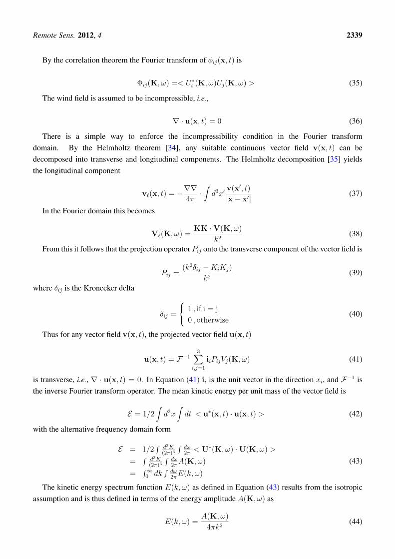
Figure 1. Diffusion coefficient D as a function of aerosol diameter Dp in µm at 20 ◦C.
10−3 10−2 10−1 100 101
10−6
10−4
10−2
D [c
m2 s
−1]
Particle Diameter Dp [µ m]
The spatial wavenumber magnitude is K = |K| = (K2x +K2
y +K2z )1/2 [ m−1]. Use a spatial grid of
dx = dy = dz = 1 m, and the digital transform relation dx dKx = 2π/Nx, where Nx is the number ofgrids in the x direction and similarly for y and z directions. It follows that K has the maximum valueKmax = 2π 31/2 = 10.9. From Figure 1, the maximum diffusion coefficient Dmax for particles withDp = 1 × 10⁻³µm is Dmax ≈ 2 × 10⁻⁶ m2/s so that KmaxDmax ≈ 2.2 × 10⁻⁵m/s. The maximumBrownian motion transport speed is four orders of magnitude less than usable surface winds. Hence thediffusion term in Equation (59) can be neglected. In the absence of diffusion and sources or sinks, theadvective solution to Equation (59), from Equations (23) and (24) is
ρ(x, t+ dt) = ρ(x− u dt, t) (61)
Remote Sens. 2012, 4 2343
Statistically the total mass density of aerosol particles is a measured quantity, i.e., the total suspendedparticulates or TSP. Reference Brook et al. [41] is based upon the Canadian National Air PollutionSurveillance network, and at the time was one of the world’s largest and most geographically diversedata sets. The average 24 h collections at 14 sites with a sample size of n = 2,831 resulted in a TSPnormal distribution N(m,σ) fit with mean m = 55µ g/m3 and standard deviation σ = 38µ g/m3. Ourwind field uses m = 100µ g/m3 and σ = 20µ g/m3.
Let ρn(x) ≡ ρ(x, tn) be the mass density at the nth time interval and ∆ρ(x) a small random sourceof aerosol particulates. Then the density model is defined as
ρn(x) = ρn−1(x− un−1(x)∆t) + ∆ρ(x) (62)
The refresh term in Equation (62) is necessary. Without it, after a few cycles, the advection processmixes the atmospheric aerosol density distribution to a non-physical featureless uniform one. Particles inthe atmosphere are continuously being created and removed by several complicated chemical processesincluding nucleation, coagulation, and Stokes sedimentation [5]. More importantly, wind blown sandand minerals lofted by saltation is a primary source of atmospheric mineral dust [42]. Recently it hasbeen discovered that the saltated particles are ionized, thus increasing this effective particle source [43].Figure 2, Whitby and Cantrell [44] gives an idealized tri-modal distribution of atmospheric aerosolsurface area as a function of particle diameter in µm. It shows how the three particle size modes interact,and contains particle sources and sinks. The particles in the accumulation range, from 0.1 to 2.5 µm,have the longest lifetimes and also represent the largest component of aerosol surface area per unitvolume of air. The coarse range particles, created from wind blown dust and biological particles as wellas anthropomorphic sources, have relatively brief lifetimes because of their larger Stokes settling time.For example particles of diameter greater than 10 µm settle with speeds greater than 10 m/h. Howeverthis mode of the particle size distribution has much larger volume backscatter coefficients for 1.5µm
laser light.In Equation (62), the initial time value ρ1(x) is chosen to be a three-dimensional (Nx, Ny, Nz)
random normally distributed array with given mean and standard deviation (mm, σm), i.e., distributedN(mm, σm) representing TSP (total suspended particulates) in units of µg/m3. As seen in Figure 2,atmospheric aerosol TSP typically contains particle diameters ranging from 0.01 to 100 µm. Mean valuemass densities are in the range 20 < mm < 200µg/m3. At later times, n = 2, 3, · · · , Nt, the densityis advected using interpolation. Points advected outside the rectangular volume are wrapped around byperiodic extension of the fundamental cell. Without the random addition of ∆ρ(x) to Equation (62),numerical diffusion would flatten the starting distribution to homogeneity. The heterogeneity of theaerosol mass density function ρn(x) makes it possible to correlate aerosol density fluctuations.
Because of the cited complicated nature of actual aerosol dust sources and their interactions, a simplead hoc source model is chosen. To maintain aerosol heterogeneity, a small amplitude of random massdensity ∆ρ(x), 3.5 percent of the mean value of TSP, is injected with random subsets of pixels intothe fundamental cell at each time frame. This amplitude value is chosen empirically to maintain thespatial bandwidth of the aerosol density images approximately constant. The injected TSP also drawsfrom distributions N(m,s). One half the points receive this injection. The grid injection points are alsoselected randomly for each cycle. For each cycle, the modified distribution is renormalized to N(m,s).

Remote Sens. 2012, 4 2344
Figure 2. Idealized schematic of atmospheric aerosol cycles including sources, sinks,particle modes and particle creation as a function of particle diameter in µm. From Whitbyand Cantrell [44].
Whitby and Cantrell, 1976
11. Streamlines
Recently, the challenge to visualize high-resolution dynamic three-dimensional vector fields in anintuitive manner has been addressed by many authors (see for example [21,22,45]). For static vectorfield visualization, high resolution spatial coherence of the vector field is displayed by using a randomtexture background with essentially zero correlation length. Line integral convolution (LIC) along thestreamlines (field lines) correlate the image along field lines, literally like the elementary experimentusing iron fillings on a piece of glass to visualize the magnetic field lines of a bar magnet placed beneaththe glass. This results in spatial coherence along flow lines. For high-resolution dynamic vector fieldvisualization, the random background texture map evolves continuously in time to support temporalcoherence [21]. Here we choose a more simple approach and use the aerosol movie density maps asbackground, and superimpose computed streamlines over the density maps.
A streamline or flow line is a path σ(x, x0), with start point x0. By definition a streamline iseverywhere tangent to the vector field v(x). Physically, a streamline is the path that a massless particlewould follow. Let x(u), y(u), z(u) be a parametric representation of a streamline. Streamlines are thussolutions to the first order vector differential equation

Remote Sens. 2012, 4 2345
dσ(u)
du= v(σ(u)) (63)
Solutions σ(u) to Equation (63) beginning at point x0 are called integral curves. It can be shown thatin regions where |v| > 0, the solutions are unique [46]. Equation (63) is simplified when the differentialparameter du is chosen as the arc length differential ds = (dx2 + dy2 + dz2)1/2. Units are chosen suchthat the speed is v = (x2
u + y2u + z2
u)1/2 resulting in
dσ(u)
ds= v(σ(u)) (64)
where v is the unit vector pointing in direction v. The start points x0 are chosen to be a randomlypermuted subset N0 of the centers of the display grid cells, and then each point is moved to a randomlocation within its cell. Numerical solutions to streamline Equation (64) typically use an error correctingRunge–Kutta algorithm [47]. Experimentation shows that a Runge–Kutta 23 solver, which comparespoint wise second and third order solutions for error correction, is a reasonable compromise betweenspeed and accuracy. For our application, the right-hand-side unit vector in Equation (64) is determined byinterpolation, in the examples to follow by two-dimensional interpolation of the velocity field estimatedon a three-dimensional grid by the spatio-temporal method. Profiling shows interpolation is the mosttime consuming task in streamline computation. In our Matlab [29] script, substitution, where possible,of interp2 by qinterp2 [48] reduces computation time by approximately a factor of six.
12. Summary of Orbiting Cloud Model
Reference [23] compares the four wind field estimation methods using a two-dimensional cloudmodel. The particle density of the cloud is Gaussian modulated, with a filtered random-like shape.The cloud background is filtered random noise. The cloud is stretched and rotated to have a prescribedaspect ratio. The centroid of the cloud moves in a circular orbit. Forty five time lapse 2D images(512 × 512 pixels) corresponding to one orbit are used to simulate a moving cloud. Eight figurescompare the true centroid velocity components (vx, vy) in units of m/s as a function of time with theestimated values (vx, vy) for each of the four methods. All comparisons are based upon the same 45image data set. Because of the circular motion, this results in a noisy sine wave versus time for vx andsimilarly a noisy cosine wave for vy. For this model, the true velocity is assumed to be defined by thecloud centroid motion. The cloud edge is modulated by a small amplitude random number input thatvaries image to image. Thus all four methods, based upon all pixel information in the images, will beaffected. Four conclusions can be drawn from this study. Firstly, SM is superior to CCM, because of theability of SM to discriminate against noise. Secondly, for STM, 2D local neighborhood median filteringyields better estimates than the equivalent 2D local neighborhood mean filtering. Thirdly, on average,SM and STM provide better estimates than CCM and TPSM. The fourth observation is that for TPSM,for this type of noisy cloud model, a global 2D Kaiser window, i.e., using segmentation parameters(Nf = 512, Nb = 1), yields more accurate estimates than the choice (Nf = 384 = 128 × 3, Nb = 6).This is because the underlying centroid motion is composed of low spatial frequencies.
Table 1 statistically summarizes the time statistics of median, mean, and standard deviation for STMvelocity estimation over the the 45 time lapse images for the velocity field parameters vx, vy and speed
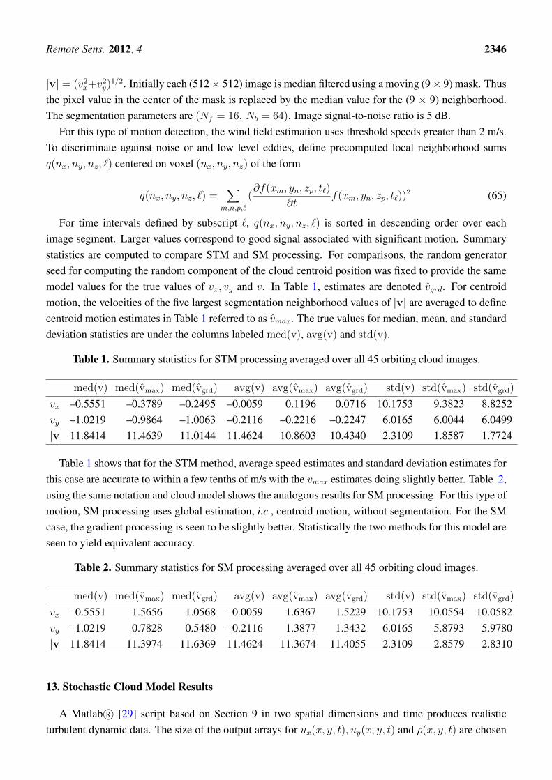
Remote Sens. 2012, 4 2346
|v| = (v2x+v2
y)1/2. Initially each (512× 512) image is median filtered using a moving (9× 9) mask. Thus
the pixel value in the center of the mask is replaced by the median value for the (9 × 9) neighborhood.The segmentation parameters are (Nf = 16, Nb = 64). Image signal-to-noise ratio is 5 dB.
For this type of motion detection, the wind field estimation uses threshold speeds greater than 2 m/s.To discriminate against noise or and low level eddies, define precomputed local neighborhood sumsq(nx, ny, nz, `) centered on voxel (nx, ny, nz) of the form
q(nx, ny, nz, `) =∑
m,n,p,`
(∂f(xm, yn, zp, t`)
∂tf(xm, yn, zp, t`))
2 (65)
For time intervals defined by subscript `, q(nx, ny, nz, `) is sorted in descending order over eachimage segment. Larger values correspond to good signal associated with significant motion. Summarystatistics are computed to compare STM and SM processing. For comparisons, the random generatorseed for computing the random component of the cloud centroid position was fixed to provide the samemodel values for the true values of vx, vy and v. In Table 1, estimates are denoted vgrd. For centroidmotion, the velocities of the five largest segmentation neighborhood values of |v| are averaged to definecentroid motion estimates in Table 1 referred to as vmax. The true values for median, mean, and standarddeviation statistics are under the columns labeled med(v), avg(v) and std(v).
Table 1. Summary statistics for STM processing averaged over all 45 orbiting cloud images.
med(v) med(vmax) med(vgrd) avg(v) avg(vmax) avg(vgrd) std(v) std(vmax) std(vgrd)
vx –0.5551 –0.3789 –0.2495 –0.0059 0.1196 0.0716 10.1753 9.3823 8.8252vy –1.0219 –0.9864 –1.0063 –0.2116 –0.2216 –0.2247 6.0165 6.0044 6.0499|v| 11.8414 11.4639 11.0144 11.4624 10.8603 10.4340 2.3109 1.8587 1.7724
Table 1 shows that for the STM method, average speed estimates and standard deviation estimates forthis case are accurate to within a few tenths of m/s with the vmax estimates doing slightly better. Table 2,using the same notation and cloud model shows the analogous results for SM processing. For this type ofmotion, SM processing uses global estimation, i.e., centroid motion, without segmentation. For the SMcase, the gradient processing is seen to be slightly better. Statistically the two methods for this model areseen to yield equivalent accuracy.
Table 2. Summary statistics for SM processing averaged over all 45 orbiting cloud images.
med(v) med(vmax) med(vgrd) avg(v) avg(vmax) avg(vgrd) std(v) std(vmax) std(vgrd)
vx –0.5551 1.5656 1.0568 –0.0059 1.6367 1.5229 10.1753 10.0554 10.0582vy –1.0219 0.7828 0.5480 –0.2116 1.3877 1.3432 6.0165 5.8793 5.9780|v| 11.8414 11.3974 11.6369 11.4624 11.3674 11.4055 2.3109 2.8579 2.8310
13. Stochastic Cloud Model Results
A Matlab R© [29] script based on Section 9 in two spatial dimensions and time produces realisticturbulent dynamic data. The size of the output arrays for ux(x, y, t), uy(x, y, t) and ρ(x, y, t) are chosen

Remote Sens. 2012, 4 2347
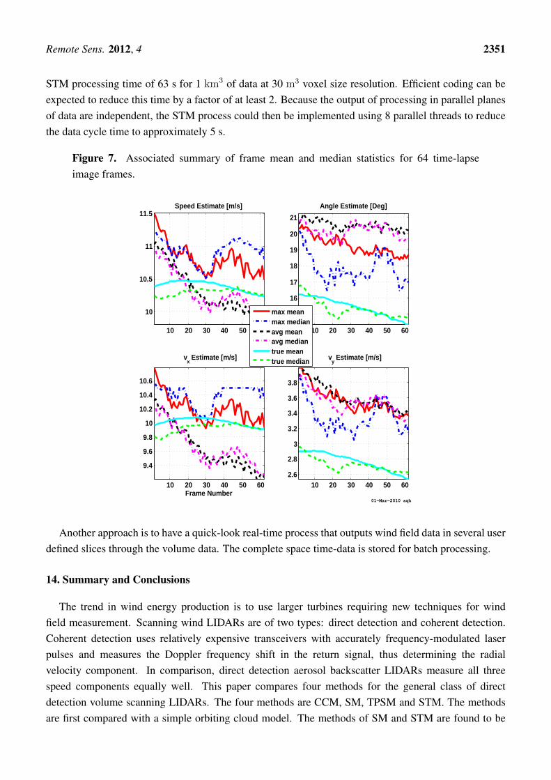
to be [640, 640, 320]. Computations use FFTs that efficiently utilize compound integers of the form640 = 5 × 27, 320 = 5 × 26). The inertial wavenumber cutoff in Equation (46) is chosen aski = 1/(4π), corresponding to large eddies of approximately 20 m as seen in Figure 3. InEquation (48), σ = 2.87. Matlab R© uses the maximally performant FFTW algorithm [49] andautomatically detects real input arrays saving almost the theoretical factor of two in space and time.Comparison of our implementation of segmented STM and SM on the stochastic cloud and data model,as developed in Section 9, shows semblance to be slightly more accurate in estimating wind fieldmagnitude and direction. We believe this is partially explained by the unique ability of semblance toanalyze both amplitude and pattern. It is also more efficient by approximately a factor of 2 because of theFFT implementation. The 3D synthetic data computation takes 22 s of CPU time on an i7 Intel computerwith 12 GB memory. Each 640 × 640 frame of motion retrieval analysis requires approximately 0.5CPU seconds. This can be improved by more efficient 2D interpolation.
Figure 3. Segmented SM processing result for one frame of stochastic cloud model data.Color bar scale aerosol density units are µg/m3.
The large scale slowly varying wind component u`(x, t) from Equation (32) is defined as
ux`(t) = 10 cos(12t/T ) ,
uy`(t) = 3.5 cos(12t/T + π/4) ,
(66)
where T = 40 s, the discrete has Nω = 320 components t = [−T/2 + dt/2 : dt : T/2 − dt/2].The wind speed units in Equation (66) are m/s. In the following examples the subset of times tn for

Remote Sens. 2012, 4 2348
64 ≤ n ≤ 128 is chosen for both large and small wind components for the dynamical simulations.Figures 3 through 7 are based on the same data set. Figure 3 shows one of 320 representative outputframes of 2D vector wind processing superimposed on bone colored aerosol density map in µg/m3.Image processing converts each 640 × 640 spatial grid to a 20 × 20 segmentation. Each of the 400resulting segments is analyzed by a 64 × 64 FFT for local semblance computation. Figure 3 has threearrow colors. Red is the true value, blue is the maximum semblance estimate and magenta gives theaveraged semblance estimate. Maximum semblance uses the velocity based on the maximum semblanceoutput. The more robust averaged estimate uses the largest 100 semblance outputs for each segment andcomputes a semblance weighted average. Color bar at right assigns gray scale to aerosol mass density.Visual inspection of Figure 3 shows the arrows for the most part overlapping. Video clip avi files of theturbulent model and vector field processing, corresponding to single frame results of Figures 3 and 4, arein file mar21 wind avi files.pdf for viewing in the same directory as the file for this paper.
Figure 4. Runge–Kutta streamline example from stochastic model using 25 start pointsshown in yellow. Cubic interpolation is used to smooth the results.
Figure 4 demonstrates the Runge–Kutta computation of streamlines. The processing selects 25 startpoints shown as yellow asterisks. The associated aerosol mass density is shown in background. Thestart points in this case are chosen to be uniformly spaced on left hand and bottom borders. Streamlinesmoothing uses five point cubic interpolation between each pair of Runge–Kutta points. The cubicsections use known end points and slopes. Figure 5 is a pixel by pixel color contour error analysisof Figure 3. Note the magnitude error has a log10 scale so that for example bright red corresponds toapproximately 10% relative error with cooler colors less. Figure 6 is a frame-by-frame average median

Remote Sens. 2012, 4 2349
analysis of 64 successive time lapse image frames. Upper right hand subplot is difference in degreesbetween true and estimated median wind direction. Averaging over all frames of turbulent motionestimation, the average median speed error is approximately 7.5%. The average median pointing error is5 degrees.
Figure 5. Associated magnitude and direction error analysis for Figure 3 data. Uppercolor bar units are log10(pe), where pe is speed percent relative error. Lower color bar unitsare degrees.
x [m], Mean Speed Error= 7.92 [%], STD = 6.966 [m/s]
y [
m]
log10
Averaged Semblance Speed Error Contours [%], t = −2.9375
−50 0 50
−50
0
50
−1.5
−1
−0.5
0
0.5
1
1.5
x [m], Mean Angle Diff = 4.13 [Deg], STD = 6.914 [Deg]
y [
m]
Averaged Semblance Angle Difference Contours [Deg], t = −2.9375
−50 0 50
−50
0
50
5
10
15
20
25
30
35
The error analysis in Figures 5 and 6 do not tell the whole story. Time-lapse techniques are proneto yield biased mean speed estimates. Figure 7 plots frame-by-frame mean and median speed as wellas component velocity statistics for 64 frames of time lapse data and compares them to the true valuesfrom the modeled wind field data. The bias for this more realistic turbulent model is evident and in thesecases is less than ±1 m/s. The bias shifts from positive to negative during the 64 frame sequence. Suchbias between anemometer and wind LIDAR are documented and explained in [1]. The idea is that windLIDAR by necessity samples a larger volume of air than a cup anemometer to infer wind speed. Near theearth, there is a positive vertical gradient of wind speed due to surface drag that is more pronounced inareas with more terrain relief. Volumetric samples near the earth are therefore biased to smaller valuesthan anemometers. The difference in measurement spatial averaging also explains the observed largerstandard deviation of anemometer wind speeds in comparison to LIDAR. Anemometers measure smallerscale turbulence that the LIDAR measurement does not see. Methods for correcting for this bias are anarea for future investigation.

Remote Sens. 2012, 4 2350
Figure 6. Associated summary median percent relative error statistics for 64 time-lapseimage frames.
20 40 60
1
2
3
4
5
6
7Avg Median Speed Relative Error %
20 40 60
4
4.2
4.4
4.6
4.8
5
5.2
5.4
5.6
Avg Median Angle Difference [Deg]
20 40 60
1
2
3
4
5
6
Avg Median vx Relative Error %
Frame Number20 40 60
26
28
30
32
34
36
Avg Median vy Relative Error %
Frame Number
01−Mar−2010 aqh
The techniques proposed here fail when the aerosol density is uniform, i.e., when there are nomeasurable fluctuations. For example if the density is nearly constant in the vicinity of a flow linefor a period of time in the volume data, velocity estimation in this vicinity by correlation is not possible.Doppler LIDAR wind and anemometers mapping remains useful in this case. Segmentation and therobust signal-to-noise-property of SM reduce, but cannot overcome, this deficiency.
Finally some words on integration of this process with hardware and applying it to 4D wind fieldestimation. Because such systems are monostatic, all signals are returned via a collecting telescope tothe detector area in the order of 0.04 mm2. Commercial 12 bit high-speed digitizers can now sample upto 2 GS/s. A cubic km of data at a resolution of 30 m3 per voxel is 3.33 × 10⁷ samples. Assume a 5 speriod for the scanning system, and 100 sample averaging. This corresponds to 0.67 GS/s. The signalaveraging can also be done on the digitizer card and then stored to a solid state drive with speeds up to500 Mb/s. All of this is at the front end of the wind field estimation process outside of the CPU. The firststep of the CPU process is to interpolate the 3D spherical coordinate data onto rectangular coordinatesas described in the introduction. Linearly scaling this interpolation time to 3.33 × 10⁷ samples yields2 s. Because the data is 12 bit, faster integer arithmetic can be used. Also, as planes of rectangular databecome available, the STM processing can begin in the populated planes. As expected, the majority oftime is spent with the velocity field estimation step. For example, as presently coded, STM processingof 512 × 512 time lapse images takes 0.5 s. Linear scaling of this time to 3.33× 10⁷ voxels predicts an
Remote Sens. 2012, 4 2351
STM processing time of 63 s for 1 km3 of data at 30 m3 voxel size resolution. Efficient coding can beexpected to reduce this time by a factor of at least 2. Because the output of processing in parallel planesof data are independent, the STM process could then be implemented using 8 parallel threads to reducethe data cycle time to approximately 5 s.
Figure 7. Associated summary of frame mean and median statistics for 64 time-lapseimage frames.
10 20 30 40 50 60
10
10.5
11
11.5Speed Estimate [m/s]
10 20 30 40 50 60
15
16
17
18
19
20
21
Angle Estimate [Deg]
10 20 30 40 50 60
9.4
9.6
9.8
10
10.2
10.4
10.6
vx Estimate [m/s]
Frame Number
max meanmax medianavg meanavg mediantrue meantrue median
10 20 30 40 50 602.6
2.8
3
3.2
3.4
3.6
3.8
vy Estimate [m/s]
01−Mar−2010 aqh
Another approach is to have a quick-look real-time process that outputs wind field data in several userdefined slices through the volume data. The complete space time-data is stored for batch processing.
14. Summary and Conclusions
The trend in wind energy production is to use larger turbines requiring new techniques for windfield measurement. Scanning wind LIDARs are of two types: direct detection and coherent detection.Coherent detection uses relatively expensive transceivers with accurately frequency-modulated laserpulses and measures the Doppler frequency shift in the return signal, thus determining the radialvelocity component. In comparison, direct detection aerosol backscatter LIDARs measure all threespeed components equally well. This paper compares four methods for the general class of directdetection volume scanning LIDARs. The four methods are CCM, SM, TPSM and STM. The methodsare first compared with a simple orbiting cloud model. The methods of SM and STM are found to be
Remote Sens. 2012, 4 2352
most accurate, with averaged mean-speed errors of 0.03 m/s for gradient weighted SM and 0.05 m/s forgradient weighted STM.
A second non-linear turbulent flow model provides for more realistic simulations and incorporates aFFT-PC based solution for the Navier–Stokes equation for isotropic and non-compressible flow. It doesnot contain terrain profile nor boundary layer effects but is nonetheless adequate for inter-comparison ofthe four retrieval methods. To simulate LIDAR backscatter data, an associated model for atmosphericaerosol density fluctuations ρ(x, y, t) is implemented. Example results using this model demonstrateprocessing algorithm validation and comparison in a simulated environment where the true vector windfield is known. Extensions to the simulated wind field incorporating earth surface drag and boundarylayer shear will result in more accurate turbulence scaling. Adding a more realistic saltation source tothe aerosol transport model is another important extension. Correction for the wind speed bias throughauxiliary measurement, extended modeling and/or image processing needs to be investigated. The wayforward is to design, build, and evaluate a suitable, eye-safe, volumetric scanning backscatter LIDARwith effective range of at least 2 km, and spatial and time resolution respectively on the order 30 m3
and 5 s.
AcknowledgmentsThe authors gratefully acknowledge USTAR funding and the support and collaboration of the CASI
and EDL staff at Utah State University that made this work possible. The first author thanks theGeophysics Department of UFPa for their support during paper revisions. We also acknowledgethe MDPI reviewers and editors for several important comments and suggestions leading to animproved paper.
References
1. Lang, S.; McKeogh, E. Lidar and sodar measurements of wind speed and directions in uplandterrain for wind energy purposes. Remote Sens. 2011, 3, 1871–1903.
2. Sela, N. The SpiDAR Wind Measurement Technique; Available online:http://www.windtech-international.com/articles/the-spidar-wind-measurement-technique(accessed on 16 July 2012).
3. Kovalev, K.; Eichinger, W. Elastic Lidar: Theory, Practice, and Analysis Methods; John Wiley &Sons, Inc.: Hoboken, NJ, USA, 2004.
4. Wilkerson, T.D.; Marchant, A.B.; Apedaile, T.J. Wind-field characterization from the trajectoriesof small balloons. J. Atmos. Ocean. Technol. 2012, In Press.
5. Seinfeld, J.; Pandis, S. Atmospheric Chemistry and Physics; John Wiley & Sons, Inc.: Hoboken,NJ, USA, 1998.
6. Eloranta, E.W.; King, J.M.; Weinman, J.A. The determination of wind speeds in the boundary layerby monostatic lidar. J. Appl. Meteorol. 1975, 14, 1485–1489.
7. Mayor, S.; Lowe, J.P.; Mauzey, C.F. Two-component horizontal aerosol motion vectors in theatmospheric surface layer from a cross-correlation algorithm applied to elastic backscatter lidardata. J. Atmos. Ocean. Technol. 2012, In Press.

Remote Sens. 2012, 4 2353
8. Hasager, C.B.; Badger, M.; Na, A.P.; Larsen, X.; Bingol, F. SAR-based wind resource statistics inthe Baltic Sea. Remote Sens. 2011, 3, 117–144.
9. De Wekker, S.F.J.; Mayor, S. Observations of atmospheric structure and dynamics in the owensvalley of California with a ground-based eye-safe, scanning aerosol lidar. J. Appl. Meteorol.Climatol. 2009, 48, 1483–1498.
10. Kunkel, K.E.; Eloranta, E.W.; Shipley, S.T. Lidar observations of the convective boundary layer.J. Appl. Meteorol. 1977, 16, 1306–1311.
11. Kunkel, K.E.; Eloranta, E.W.; Weinman, J.A. Remote determination of winds, turbulence spectraand energy dissipation rates in the boundary layer from lidar measurements. J. Atmos. Sci. 1980,37, 978–985.
12. Piironen, A.K.; Eloranta, E.W. Accuracy analysis of wind profiles calculated from volume imaginglidar data. J. Geophys. Res. 1995, 100, 559–567.
13. Sroga, J.T.; Eloranta, E.W.; Barber, T. Lidar measurements of wind velocity profiles in the boundarylayer. J. Appl. Meteorol. 1980, 19, 598–605.
14. Sasano, Y.; Hirohara, H.; Yamasaki, T.; Shimizu, H.; Takeuchi, N.; Kawamura, T. Horizontal windvector determination from the displacement of aerosol distribution patterns observed by a scanninglidar. J. Appl. Meteorol. 1982, 21, 1516–1523.
15. Hooper, W.P.; Eloranta, E.W. Lidar measurements of wind in the planetary boundary layer: Themethod, accuracy and results from joint measurements with radiosonde and kytoon. J. Appl.Meteorol. 1986, 25, 990–1001.
16. Kolev, I.; Parvanov, O.; Kaprielov, B. Lidar determination of winds by aerosol inhomogeneities:Motion velocity in the planetary boundary layer. Appl. Opt. 1988, 27, 2524–2531.
17. Schols, J.L.; Eloranta, E.W. The calculation of area-averaged vertical profiles of the horizontalwind velocity from volume-imaging lidar data. J. Geophys. Res. 1992, 97, 18395–18407.
18. Mayor, S.; Eloranta, E.W. Two-dimensional vector wind fields from volume imaging lidar data.J. Appl. Meteorol. 2001, 40, 1331–1346.
19. Stam, J.; Fuime, E. Turbulent Wind Fields for Gaseous Phenomena. In Proceedings of the 20thAnnual Conference on Computer Graphics and Interactive Techniques, SIGGRAPH’93, Anaheim,CA, USA, 2–6 August 1993; pp. 369–376.
20. Stam, J. A simple fluid solver based on the FFT. J. Graph. Tools 2001, 6, 43–52.21. Sundquist, A. Dynamic line integral convolution for visualizing streamline evolution. IEEE Trans.
Vis. Comput. Graph. 2003, 9, 273–282.22. Weiskopf, D.; Eriebacher, G.; Ertl, T. A Texture-Based Framework for Spacetime-Coherent
Visualization of Time-Dependent Vector Fields. In Proceedings of IEEE Visualization 2003,Seattle, WA, USA, 19–24 October 2003; pp. 107–114.
23. Marchant, A.B.; Barson, R.L.; Wojcik, M.; Howard, A.Q. Dynamic 3D Wind Mapping System andMethod. US Patent 0149268 A1, 23 June 2011.
24. Oppenheim, A.; Schafer, R. Discrete-Time Signals and Systems. In Digital Signal Processing;Prentice Hall, Inc.: Englewood Cliffs, NJ, USA, 1975; pp. 242–244.
25. Tittman, J. The Physics of Logging Measurements. In Geophysical Well Logging; Academic Press,Inc.: Orlando, FL, USA, 1986; pp. 164–165.
Remote Sens. 2012, 4 2354
26. Lim, J.S. Image Enhancement. In Two-Dimensional Signal and Image Processing; Prentice HallPTR: Upper Saddle River, NJ, USA, 1990; pp. 503–506.
27. Tolman, R.C. Statistical Ensembles in the Classical Mechanics. In The Principles of StatisticalMechanics; Oxford University Press: Oxford, UK, 1962; pp. 43–54.
28. Golub, G.H.; Loan, C.V. Special Topics. In Matrix Computations, 2nd ed.; The John HopkinsUniversity Press: Baltimore, MD, USA, 1989; pp. 579–633.
29. The Mathworks, Inc. Matlab R©; Available online: www.mathworks.com (accessed on 2 August2012).
30. Stull, R.B. Application of the Governing Equations to Turbulent Flow. In An Introduction toBoundary Layer Meteorology; Kluwer Academic Publishers: Dordrecht, The Netherlands, 1988;pp. 75–114.
31. Lesieur, M. Fourier Analysis of Homogeneous Turbulence. In Turbulence in Fluids, Stochastic andNumerical Modelling, 2nd ed.; Kluwer Academic Publishers: Dordrecht, The Netherlands, 1990;pp. 137–138.
32. Kaimal, J.C.; Finnigan, J.J. Atmospheric Boundary Layer Flows: Their Structure andMeasurement; Oxford University Press: New York, NY, USA, 1994.
33. Kaimal, J.C.; Wyngaard, J.C.; Izumi, Y.; Cote, O.R. Spectral characteristics of surface-layerturbulence. Quart. J. Roy. Meteorol. Soc. 1972, 98, 563–589.
34. Arfken, G. Vector Analysis. In Mathematical Methods for Physicists, 2nd ed.; Academic Press:New York, NY, USA, 1970; pp. 66–67.
35. Howard, A.Q., Jr. On the longitudinal component of the green’s function Dyadic. Proc. IEEE1974, 62, 1704–1705.
36. Knight, B.; Sirovich, L. Kolmogorov inertial range for inhomogeneous turbulent flows. Phys. Rev.Lett. 1990, 65, 1356–1359.
37. Bowman, J. On inertial-range scaling laws. J. Fluid Mech. 1996, 306, 167–181.38. Lu, R.; Turco, R.; Jacobson, M. An integrated air pollution modeling system for urban and regional
scales: I. Structure and performance. J. Geophys. Res. 1997, 102, 6063–6079.39. Costabile, F.; Birmilli, W.; Klose, S.; Tuch, T.; Wehner, B.; Wiedensohler, A.; Franck, U.;
Konig, K.; Sonntag, A. Spatio-temporal variability and principal components of particle numbersize distribution in an urban atmosphere. Atmos. Chem. Phys. 2009, 9, 3163–3195.
40. Stocker, T. Introduction to Climate Change; Springer: New York, NY, USA, 2011.41. Brook, J.; Dann, T.; Burnett, R. The relationship among TSP, PM10, PM2.5, and inorganic
constituents of atmospheric particulate matter at multiple Canadian locations. J. Air Waste Manage.Assoc. 1997, 47, 2–19.
42. Field, J.; Belnap, J.; Breshears, D.D.; Neff, J.C.; Okin, G.S.; Whicker, J.J.; Painter, T.H.; Ravi, S.;Reheis, M.C.; Reynolds, R.L. The ecology of dust. Front. Ecol. Environ. 2010, 8, 423–430.
43. Kok, J.F.; Renno, N.O. Electrostatics in wind-blown sand. Phys. Rev. Lett. 2008, 100, 014501.44. Whitby, K.; Cantrell, B. Fine Particles. In Proceedings of International Conference on
Environmental Sensing and Assessments, Las Vegas, NV, USA, 14–19 September 1975.45. Shen, H.W.; Kao, D. A new line integral convolution algorithm for visualizing time-varying flow
fields. IEEE Trans. Vis. Comput. Graph. 1998, 4, 98–108.

Remote Sens. 2012, 4 2355
46. O’Neill, B. Elementary Differential Geometry; Academic Press: New York, NY, USA, 1966.47. Moler, C.B. Numerical Computing with Matlab; SIAM: Philadelphia, PA, USA, 2004.48. Brahms, N. Fast 2-Dimensional Interpolation; Available online: http://www.mathworks.com/
matlabcentral/fileexchange/10772 (accessed on 31 May 2006).49. Frigo, M.; Johnson, S. The design and implementation of FFTW3. Proc. IEEE 2005, 93, 213–216.
c© 2012 by the authors; licensee MDPI, Basel, Switzerland. This article is an open access articledistributed under the terms and conditions of the Creative Commons Attribution license(http://creativecommons.org/licenses/by/3.0/).