Non-Contact Microscale Manipulation using laser-induced ...
103
HAL Id: tel-00647226 https://tel.archives-ouvertes.fr/tel-00647226 Submitted on 1 Dec 2011 HAL is a multi-disciplinary open access archive for the deposit and dissemination of sci- entific research documents, whether they are pub- lished or not. The documents may come from teaching and research institutions in France or abroad, or from public or private research centers. L’archive ouverte pluridisciplinaire HAL, est destinée au dépôt et à la diffusion de documents scientifiques de niveau recherche, publiés ou non, émanant des établissements d’enseignement et de recherche français ou étrangers, des laboratoires publics ou privés. Non-Contact Microscale Manipulation using laser-induced convection flows Emir Augusto Vela Saavedra To cite this version: Emir Augusto Vela Saavedra. Non-Contact Microscale Manipulation using laser-induced convection flows. Automatic. Université Pierre et Marie Curie - Paris VI, 2010. English. tel-00647226
-
Upload
khangminh22 -
Category
Documents
-
view
2 -
download
0
Transcript of Non-Contact Microscale Manipulation using laser-induced ...

HAL Id: tel-00647226https://tel.archives-ouvertes.fr/tel-00647226
Submitted on 1 Dec 2011
HAL is a multi-disciplinary open accessarchive for the deposit and dissemination of sci-entific research documents, whether they are pub-lished or not. The documents may come fromteaching and research institutions in France orabroad, or from public or private research centers.
L’archive ouverte pluridisciplinaire HAL, estdestinée au dépôt et à la diffusion de documentsscientifiques de niveau recherche, publiés ou non,émanant des établissements d’enseignement et derecherche français ou étrangers, des laboratoirespublics ou privés.
Non-Contact Microscale Manipulation usinglaser-induced convection flows
Emir Augusto Vela Saavedra
To cite this version:Emir Augusto Vela Saavedra. Non-Contact Microscale Manipulation using laser-induced convectionflows. Automatic. Université Pierre et Marie Curie - Paris VI, 2010. English. �tel-00647226�

NON-CONTACT MICROSCALE MANIPULATION
USING LASER-INDUCED CONVECTION FLOWS
THESE
presentee a
L’UNIVERSITE PIERRE ET MARIE CURIE
ECOLE DOCTORALE 391
SMAER Sciences Mecaniques, Acoustique, Electronique et Robotique de Paris
par
Emir Augusto VELA SAAVEDRA
pour l’obtention du grade de
DOCTEUR DE L’UNIVERSITE
PIERRE ET MARIE CURIE
Specialite:Mecanique - Robotique
A soutenir le 28 mai 2010
JURY
Mr. Charles BAROUD Professeur a l’Ecole Polytechnique RapporteurMr. Pierre LAMBERT Professeur a l’Universite Libre de Bruxelles RapporteurMr. Stephane ZALESKI Professeur a l’Universite Pierre et Marie Curie ExaminateurMr. Yves BELLOUARD Professeur a l’Universite Technologique d’Eindhoven ExaminateurMr. Moustapha HAFEZ Docteur-Ingenieur CEA LIST Co-directeur de these
Mr. Stephane REGNIER Professeur a l’Universite Pierre et Marie Curie Directeur de these


Contents
Contents ii
List of Figures vii
List of Tables ix
Notations xi
Introduction 1
1 Non-contact micromanipulation 3
1.1 Electric field driven effects . . . . . . . . . . . . . . . . . . . . . . . . . . . . . . . 5
1.2 Dielectrophoresis . . . . . . . . . . . . . . . . . . . . . . . . . . . . . . . . . . . . 6
1.3 Optical tweezers . . . . . . . . . . . . . . . . . . . . . . . . . . . . . . . . . . . . 11
1.4 Electrowetting . . . . . . . . . . . . . . . . . . . . . . . . . . . . . . . . . . . . . 14
1.5 Magnetic manipulation . . . . . . . . . . . . . . . . . . . . . . . . . . . . . . . . . 14
1.6 Acoustic waves . . . . . . . . . . . . . . . . . . . . . . . . . . . . . . . . . . . . . 17
1.7 Manipulation via actuated flows . . . . . . . . . . . . . . . . . . . . . . . . . . . 18
1.8 Summary . . . . . . . . . . . . . . . . . . . . . . . . . . . . . . . . . . . . . . . . 20
1.9 Conclusions . . . . . . . . . . . . . . . . . . . . . . . . . . . . . . . . . . . . . . . 22
2 Opto-fluidic actuation for non-contact micromanipulation 23
2.1 Theoretical background . . . . . . . . . . . . . . . . . . . . . . . . . . . . . . . . 23
2.1.1 The fluid mechanics laws . . . . . . . . . . . . . . . . . . . . . . . . . . . 24
2.1.2 Hypothesis on the model . . . . . . . . . . . . . . . . . . . . . . . . . . . 25
2.1.3 Dimensionless numbers . . . . . . . . . . . . . . . . . . . . . . . . . . . . 26
2.2 Natural convection . . . . . . . . . . . . . . . . . . . . . . . . . . . . . . . . . . . 29
2.2.1 The microfluidic system . . . . . . . . . . . . . . . . . . . . . . . . . . . . 29
2.2.2 Simulations . . . . . . . . . . . . . . . . . . . . . . . . . . . . . . . . . . . 31
2.2.3 Comparison to experimental measurements of flows . . . . . . . . . . . . . 33
2.3 Thermocapillary convection . . . . . . . . . . . . . . . . . . . . . . . . . . . . . . 36
2.3.1 Surface tension . . . . . . . . . . . . . . . . . . . . . . . . . . . . . . . . . 36
2.3.2 Marangoni effect . . . . . . . . . . . . . . . . . . . . . . . . . . . . . . . . 36
2.3.3 Working principle . . . . . . . . . . . . . . . . . . . . . . . . . . . . . . . 37
2.3.4 Formulation . . . . . . . . . . . . . . . . . . . . . . . . . . . . . . . . . . . 38
2.4 Conclusions . . . . . . . . . . . . . . . . . . . . . . . . . . . . . . . . . . . . . . . 40

ii Contents
3 Experimental analysis of thermal-induced convection flows 41
3.1 Introduction . . . . . . . . . . . . . . . . . . . . . . . . . . . . . . . . . . . . . . . 413.2 Experimental set-up . . . . . . . . . . . . . . . . . . . . . . . . . . . . . . . . . . 41
3.2.1 Microheat source: Infrared laser λ = 1480 nm . . . . . . . . . . . . . . . . 423.2.2 2-DOF mirror scanner . . . . . . . . . . . . . . . . . . . . . . . . . . . . . 433.2.3 Sample preparation . . . . . . . . . . . . . . . . . . . . . . . . . . . . . . 46
3.3 Experimental analysis of convection flows . . . . . . . . . . . . . . . . . . . . . . 473.3.1 The disturbed fluidic zone . . . . . . . . . . . . . . . . . . . . . . . . . . . 473.3.2 Velocity measurements . . . . . . . . . . . . . . . . . . . . . . . . . . . . . 473.3.3 Influence of larger beads . . . . . . . . . . . . . . . . . . . . . . . . . . . . 533.3.4 Micro-objects floating on the water-air interface . . . . . . . . . . . . . . . 543.3.5 Estimation of the manipulation force . . . . . . . . . . . . . . . . . . . . . 56
3.4 Conclusions . . . . . . . . . . . . . . . . . . . . . . . . . . . . . . . . . . . . . . . 60
4 Toward a fully automated vision-based opto-fluidic system for non-contact
micromanipulation 61
4.1 Vision feedback for micromanipulation . . . . . . . . . . . . . . . . . . . . . . . . 624.1.1 Optical flow . . . . . . . . . . . . . . . . . . . . . . . . . . . . . . . . . . . 624.1.2 Image segmentation . . . . . . . . . . . . . . . . . . . . . . . . . . . . . . 624.1.3 Hough transform . . . . . . . . . . . . . . . . . . . . . . . . . . . . . . . . 634.1.4 Image correlation . . . . . . . . . . . . . . . . . . . . . . . . . . . . . . . . 64
4.2 System calibration . . . . . . . . . . . . . . . . . . . . . . . . . . . . . . . . . . . 654.3 Micromanipulation: Operation modes . . . . . . . . . . . . . . . . . . . . . . . . 69
4.3.1 Manual operation mode . . . . . . . . . . . . . . . . . . . . . . . . . . . . 694.3.2 Automatic operation mode . . . . . . . . . . . . . . . . . . . . . . . . . . 73
4.4 Conclusions . . . . . . . . . . . . . . . . . . . . . . . . . . . . . . . . . . . . . . . 79
Conclusions and Perspectives 81
Bibliography 83

List of Figures
1.1 Assembly at all-scales. . . . . . . . . . . . . . . . . . . . . . . . . . . . . . . . . . 3
1.2 Electric field driven effects. (a) Electrophoresis. (b) DC electroosmosis. (c)Dielectrophoresis (d) AC electro-hydrodynamics. . . . . . . . . . . . . . . . . . . 6
1.3 Principle of dielectrophoresis . . . . . . . . . . . . . . . . . . . . . . . . . . . . . 7
1.4 Trapping and manipulation of a polystyrene bead. (a) Bead follows the minimumregion of electric field by selectively energizing the post shaped electrodes. (b)Simulations of the minimum region of electric field. The arrows indicate thedirection of the trap motion. . . . . . . . . . . . . . . . . . . . . . . . . . . . . . 8
1.5 Trapping in an AC octode cage field. (a) Latex bead 15 µm in diameter. (b)Latex beads 0.954 µm in diameter. . . . . . . . . . . . . . . . . . . . . . . . . . . 8
1.6 Spiral electrodes used for sorting of cells infected with malaria (in the center ingreen) . . . . . . . . . . . . . . . . . . . . . . . . . . . . . . . . . . . . . . . . . . 9
1.7 Sorting technique which combines dielectrophoresis and hydrodynamic forces. . . 9
1.8 Particle sorting using a combination of dilectrophoresis and hydrodynamic forces. 10
1.9 Capture of micro-objects above electrodes . . . . . . . . . . . . . . . . . . . . . . 10
1.10 Use of dielectrophoresis in the nanomanipulation of carbon nanotubes . . . . . . 11
1.11 Principle of optical forces. (a) Change of light momentum generating a forcegradient. (a1) Gradient light profile directed to the right hand. (a2) Gradientlight profile directed to the center. A vector diagram of the change of moment forthe left and right ray is shown. (b) Diagram of the ray-optic theory. The axis ofthe scattering force is parallel to the beam and gradient force is perpendicular. Ran T are the index of reflexion and refraction respectively, P is the laser power, θthe incident angle, ǫ the angle of refraction, ϕ the cone’s half angle of the incidentbeam, n the normal vector surface, rap the aperture radius and f is the focus ofthe lens. . . . . . . . . . . . . . . . . . . . . . . . . . . . . . . . . . . . . . . . . . 11
1.12 Optical tweezers setup. . . . . . . . . . . . . . . . . . . . . . . . . . . . . . . . . . 12
1.13 Manipulation of micro spherical beads by optical tweezers . . . . . . . . . . . . . 13
1.14 Microassembly of cells and polystyrene beads with the help of optical tweezers. . 14
1.15 Electrowetting on insulator (EWOD). (a) Principle of the EWOD, droplet sand-wiched between insulator layers deposited on both electrode plates, the insulatorsdecrease the wettability. A surface tension gradient is electrically generated fordriven the droplet toward the active electrode. V is the voltage, U is the averagetransport velocity, τ is the surface tension and Fm is the electrostatic driven forceper unit length. (b) snapshots of a moving droplet at 33 ms intervals. A 80 Vpotential is applied to the right electrode and droplet follows. . . . . . . . . . . . 15

iv LIST OF FIGURES
1.16 Magnetic manipulation. (a) Sequence of images showing the transport of a yeastcell by changing in steps the localized magnetic field controlled by currents in thewires. Y is yeast cell and M is magnetic bead. (b) Simulations of the magneticfield peak at the yeast position within the wire matrix. . . . . . . . . . . . . . . . 16
1.17 Principle of magnetic sorting of cells. . . . . . . . . . . . . . . . . . . . . . . . . . 16
1.18 Principle of cell sorting by magnetophoresis (Furlani, 2007). . . . . . . . . . . . . 17
1.19 Manipulation of fluorescent polystyrene beads of 1.9 µm in diameter. (a:a) Con-cept for 1D acoustic system. (a:b) 2D acoustic system. (b:a) 1D acoustic system.(b:b) Perpendicular arrangement of IDTs for 2D manipulation. (b:c) 1D arrange-ment of beads. (b:d) 2D arrangement of beads. . . . . . . . . . . . . . . . . . . . 18
1.20 Droplet manipulation in one degree of freedom. (a) Apparatus of the fluidicmanipulation. (b) Snapshots of the oil droplet displacement. Scale bar 100 µm . 19
1.21 Device concept . . . . . . . . . . . . . . . . . . . . . . . . . . . . . . . . . . . . . 19
1.22 Microfluidic platforms . . . . . . . . . . . . . . . . . . . . . . . . . . . . . . . . . 20
2.1 Fluid particle in cylindrical coordinates. . . . . . . . . . . . . . . . . . . . . . . . 24
2.2 Laser absorption by a liquid layer . . . . . . . . . . . . . . . . . . . . . . . . . . . 25
2.3 The system is a petri dish with a laser heating source at its center. Distilled waterfills the dish with a depth of 1.650 mm. . . . . . . . . . . . . . . . . . . . . . . . 29
2.4 Model of an objective: magnification and focusing of the light beam. . . . . . . . 30
2.5 Triangular mesh of the finite element solver. The symmetry axis is highlighted ingreen. The upper figure represents the whole chamber and the below figure is azoom view around the laser spot. . . . . . . . . . . . . . . . . . . . . . . . . . . . 31
2.6 Velocity field plotted with arrows. Axis units are in meters. . . . . . . . . . . . . 32
2.7 Radial speed plotted in contours in m/s. The maximum radial speed in thedirection of the laser is highlighted by a dotted line. Axis units are in meters. . . 32
2.8 Supperposition of 10 images during a laser group manipulation of hollow glassbeads. Those images were used to localized the particles in function of time andevaluate their speed. . . . . . . . . . . . . . . . . . . . . . . . . . . . . . . . . . . 33
2.9 The mesh quality refers to triangle angles. For example, a equilateral triangle isequal to 1. If the triangle’s angles are inferior to 90◦, the solution will be continuous. 34
2.10 Temperature field in Kelvin. Axis units are in meters. . . . . . . . . . . . . . . . 34
2.11 Radial speed in function of the radius and height position of the particles. Theexperimental data are plot with solid lines and the simulation data with dashcurves. . . . . . . . . . . . . . . . . . . . . . . . . . . . . . . . . . . . . . . . . . . 35
2.12 Three-dimensional simulation of the fluid trajectories in the fluid chamber witha laser heating source at its center. . . . . . . . . . . . . . . . . . . . . . . . . . . 35
2.13 Hexagonal pattern formation at the free surface observed in Benard convection. . 37
2.14 Schematic depicting the Benard-Marangoni convection. Convective cells are shownby the arrows. . . . . . . . . . . . . . . . . . . . . . . . . . . . . . . . . . . . . . . 37
2.15 Principle of thermocapillary manipulation. (a) IR laser absorption heats a thinfilm of liquid from below, therefore a convective flow is generated by a surfacetension gradient. (b) A 3D representation of the localized flows. (c) Velocityprofile of the convection flow in a thin liquid layer heated from below. A micro-bead immersed within the liquid is reached by a velocity profile that drags ittoward the laser focus. The arrow above the bead represents the motion direction. 38
3.1 Experimental set-up. Inset: close-up view of the microscope left part. . . . . . . 42
3.2 Water absorption spectrum. The dotted lines show the absorption coefficient fora wavelength of 1480 nm . . . . . . . . . . . . . . . . . . . . . . . . . . . . . . . . 43
LIST OF FIGURES v
3.3 TIP/TILT laser scanner. (a) Compact mechatronic device actuated by four elec-tromagnets. (b) Cross view showing the forces exerted F by the electromagneticactuators in a push-pull configuration. (c) The laser scanner prototype. . . . . . 44
3.4 TIP/TILT laser scanner mounted on the inverted microscope, under the nosepiece. 44
3.5 Experimental set-up. An IR laser 1480nm is directed by a 2-DOF laser scannerto the microscope objective to be focused on the petri dish bottom surface. Thelaser scanner also allows the imaging light to pass toward a high-speed camera. . 45
3.6 Frequency response of the laser scanner. . . . . . . . . . . . . . . . . . . . . . . . 46
3.7 Picture of a convection cell within 450 µm of water depth. At the center, theaccumulation of beads show the laser position. Hollow glass beads in the rangeof 8 up to 12 µm are used as tracers. . . . . . . . . . . . . . . . . . . . . . . . . . 48
3.8 Fluidic flow radius vs different water depths. The radius increases with the waterdepth. Error bars are taken over ten measurements. . . . . . . . . . . . . . . . . 49
3.9 Convection cell build-up while irradiating with an IR laser. The laser position isat the center of the convection cell. Every picture is shown at 110 ms of intervals.The water depth is 150 µm and particles used as tracers are hollow glass beadsof 8-12 µm in diameter. . . . . . . . . . . . . . . . . . . . . . . . . . . . . . . . . 49
3.10 Image sequences for velocity measurements of a spherical glass bead with 92µmin diameter and within 600µm of water depth. One image every 212.5ms isshown. (3.10a) Sequence taken at 80Hz. (3.10b) Image processing to determinethe velocity field between the laser and bead. The mass center is obtained fromthe white region for each image, and then the distance between two successivemas center is computed and multiplied by the frame rate. Scale bar 100µm. . . . 50
3.11 Velocity of a glass bead with 92µm in diameter vs the radial distance of the beadcenter to the laser focus (origin) with 3 different water depths. . . . . . . . . . . 51
3.12 Velocity of 3 different glass beads of 92, 62, 31 µm in diameter vs the radialdistance to the laser focus. . . . . . . . . . . . . . . . . . . . . . . . . . . . . . . 51
3.13 Velocity of glass beads with 92 and 31 µm in diameter for 600 µm water depth vsthe radial distance to the laser focus. Error bar is calculated over ten measurements. 52
3.14 Peak velocity of glass beads 31, 62, 71, 79, 92µm in diameter respectively forthree different water depth of 375, 450, 600µm. . . . . . . . . . . . . . . . . . . . 53
3.15 Illustration of the fluid velocity profile with respect to microbeads size. Aroundthe free surface, flows go away from the heat source (IR laser beam), aroundthe reservoir bottom surface flows are directed toward the laser beam. Keepingthe water depth constant, a microbead can be dragged either by the bottomsubsurface flows or also by the top subsurface flows. . . . . . . . . . . . . . . . . 54
3.16 Velocity profile of a 240 µm glass bead for 250, 300 and 450 µm of water depth.The bead is placed at about 550 µm from the laser focal point. The laser isswitched on during 100 ms. . . . . . . . . . . . . . . . . . . . . . . . . . . . . . . 55
3.17 Illustration of the convection flow profile with respect to floating microbeads in athin water layer. If a microbead bead size is comprised within the top subsurfaceflows (TSF), the bead is pushed away from the heat source. For a much largermicrobead, the bottom subsurface (BSF) flows acts also the bead and this one isdragged toward the laser beam. . . . . . . . . . . . . . . . . . . . . . . . . . . . . 55

vi LIST OF FIGURES
3.18 Image sequence showing the displacement of a floating glass bead of 180 µm indiameter. The dashed circles illustrate the bead-air interface. The white regionis a focused red laser and indicates the IR laser shot. Every image is shown atintervals of 33.3 ms. (a) The microbead goes away from laser beam within 450 µmin water depth. (b) The microbead goes toward the laser bead within 265 µm inwater depth. . . . . . . . . . . . . . . . . . . . . . . . . . . . . . . . . . . . . . . 56
3.19 Schematic of the forces involved for the estimation of the fluidic forces exerted ona spherical microbead within a liquid medium. . . . . . . . . . . . . . . . . . . . 57
3.20 Net force computed with the bead center of mass acceleration (cf. Eq. 3.1). Aglass bead of 92 µm in diameter is used within 450 µm in water depth. Theacceleration data is taken by deriving twice the bead position. . . . . . . . . . . . 57
3.21 Estimation of the force that the flows exerted on a 92µm-sized glass according toEq. 3.8. . . . . . . . . . . . . . . . . . . . . . . . . . . . . . . . . . . . . . . . . . 59
3.22 Estimation of the flows velocity distribution that drags a 92µm-sized glass im-mersed in a water depth of 450 µm according to Eq. 3.8. . . . . . . . . . . . . . 59
4.1 Image segmentation of cells (Chen et al., 2006). It shows the separation of featureswith different advanced segmentation techniques . . . . . . . . . . . . . . . . . . 63
4.2 Micro-sphere detection using the Hough transform (Pawashe & Sitti, 2006). Inthe left hand side the parametric space is shown and in the right hand side themicro-spheres detected with its respective localization (drawn circles) are depicted. 64
4.3 Images of a correlation method applied to track a glass spherical bead. Thebottom image is the result of the correlation method applied to the top image.In the top right corner the template is shown. . . . . . . . . . . . . . . . . . . . . 65
4.4 Block schemes illustrating the calibration process where the polynomial approxi-mation is used. . . . . . . . . . . . . . . . . . . . . . . . . . . . . . . . . . . . . . 66
4.5 Simulation of geometrical distortions. If a square reference is sent to the laserscanner, a curve quadrilateral is obtained on the sample due to the scanner’sdistortions. . . . . . . . . . . . . . . . . . . . . . . . . . . . . . . . . . . . . . . . 67
4.6 Superposition of eight images containing the reference laser positions on the sam-ple. (a) Background image subtraction to detect the IR laser positions. (b) Imagebinarization of each point found after background subtraction. Then morphologi-cal operations are used to improve the image quality. Computation of the objects’center of mass using OpenCV. . . . . . . . . . . . . . . . . . . . . . . . . . . . . 67
4.7 The calibration process allows to obtain a line reference on the sample (squaremarks) by sending a curve trajectory (circle marks) to the laser scanner. Thiscurve is determined by a polynomial approximation. . . . . . . . . . . . . . . . . 68
4.8 Flow chart illustrating the system calibration process. . . . . . . . . . . . . . . . 68
4.9 Representation scheme of the manual operation mode. . . . . . . . . . . . . . . . 70
4.10 Pictures depicting the manipulation of beads. (a) Separation of three beads of 75to 85 µm in diameter. The red dot is the laser position. b) Trapping of micro-spheres inside a laser circular pattern. Glass beads of 75 to 85 µm in diameter.. . . . . . . . . . . . . . . . . . . . . . . . . . . . . . . . . . . . . . . . . . . . . . 71
4.11 Annular PZT piezo-transducer is glued on a petri dish. It engenders acousticvibrations to push the micro-parts up from the substrate. (a) View of the petridish bottom surface. (b) Side view of petri dish and transducer. . . . . . . . . . 71
4.12 Manipulation of non-spherical parts. (a) Silicon cubes of 100 µm in size aredragged. (b) Silicon parts of 200 µm as maximum side are being grouped. Thewhite dot is the laser position. . . . . . . . . . . . . . . . . . . . . . . . . . . . . 72

List of Figures vii
4.13 Pictures depicting the manipulation of large and heavy micro-parts. (a) Lead-tinsolder bead of 200 µm in diameter is dragged. (b) Manipulation of a capacitor of400 × 200 × 50 µm3 in size. A PZT transducer is used to reduce the adhesionsforces with the glass substrate. . . . . . . . . . . . . . . . . . . . . . . . . . . . . 73
4.14 Flow chart illustrating the control algorithm used for automation. . . . . . . . . 754.15 Block diagram of the implemented multithreaded program. The main program
is divided into three independent programs which communicates between eachother with shared and protected variables. I0,1 and P0,1 are images and positionshared variables. . . . . . . . . . . . . . . . . . . . . . . . . . . . . . . . . . . . . 76
4.16 Representation scheme of the tracking method using image correlation. The laseris shot to drag the bead, the bead moves and the ROI updates its position to findthe bead. Once the bead position is computed, the laser is shot. . . . . . . . . . 76
4.17 Image sequence depicting the automatic manipulation of two beads. (a) The beadpositions are detected by the program. (b) The user introduces the respective goalpositions with a computer mouse by only clicking on the image frame. (c-h) TheIR laser is shot by switching from one bead to the other till the beads arrive todestination. The pictures are shown at intervals of 1 s. Scale bar of 200 µm . . . 78

viii List of Figures
List of Tables
1.1 Comparisons of non-contact micromanipulation methods . . . . . . . . . . . . . . 21
2.1 Thermophysical properties of liquid water (Straub, 1993) . . . . . . . . . . . . . 282.2 Boundary conditions . . . . . . . . . . . . . . . . . . . . . . . . . . . . . . . . . . 30
4.1 Comparisons of image processing methods . . . . . . . . . . . . . . . . . . . . . . 65

x List of Tables
Notations
σ = σij Total stress tensor [N m−2]
Fs Forces acting in surfaces or Stress forces [N ]
Fv Body Forces [N ]
∇ =∂
∂xiGradient operator [m−1]
x = xi coordinate system [m]
u = ui Velocity field of the fluid [m s−1]
∂S Surface of a fluid particle [m2]
∂V Volume of the fluid particle [m3]
β Coefficient of thermal expansion [K−1]
γ Surface tension [N m−1]
κ Thermal diffusivity [m2s−1]
µ = ρν Dynamic viscosity [N s m−2]
ν Cinematic viscosity [m2 s−1]
ρ =∂m
∂VDensity [kg m−3]
b Superficial tension’s temperature variation rate [K−1]
Cp Specific heat at constant pressure [J kg−1 K−1]
m Mass [kg]
ρ0 Referential density [kg m−3]
L Characteristic length [m]
U Characteristic velocity [ms−1]
λ Laser wavelength [m]
I Radiation intensity [W m2]
Ql Volumetric heat flux induced by the laser absorption [J s−1]

xii Notations

Introduction
This work relates to the automated parallel manipulation of parts at sub-millimeter scale andis a part of EU funded GOLEM Project. The main challenge at this scale is to develop novelmethods for high throughput parallel assembly of components of a few hundreds of micrometers.At this scale, a serial approach would be extremely limited by the requirements on precision,speed ans especially by the particularities of physics.
The proposed approach in this work is opto-fluidic, based on the Marangoni effect, a con-vective fluidic phenomena. The Marangoni effect is explored and analyzed both theoreticallyand experimentally. An experimental set-up is designed and constructed in this purpose. Thesestudies show the advantages of the proposed approach for high speed manipulation of micro-components in different sizes and geometries. The manipulation set-up is also entirely automatedin order to show the parallel manipulation capabilities of this novel assembly technique.
The first chapter gives an overview of contactless manipulation techniques at microscale,such as optical tweezers, electric field, dielectrophoresis, acoustic waves and thermal motionbased techniques. A comparison of the techniques points Marangoni effect as a viable solution.
The second chapter deals with the theoretical analysis of two convection phenomena: freeconvection and Benard-Marangoni convection. This through a multi-physics finite elementsbased modeling. The governing equations for these phenomena are presented based on the fluiddynamics laws. A Proposed model is applied on a simple case of natural convection for initialanalysis. Several simulations and their experimental validations are presented. Different pa-rameters are analyzed such as water depth, temperature distribution and velocity field. Finally,a comparison between these phenomena is presented to know which mechanism predominatesand is more suitable in our case. The Marangoni effect is presented as a promising methodto drag micro-objects immersed in liquid media using only an IR laser beam as a heat source.This analysis allowed us to define the parameters for a conception of an experimental set-up fornon-contact manipulation.
The third chapter describes the design of this above mentioned robotic platform. This plat-form is composed of several components: an optical microscope, a laser source as local thermalsource, a scanner to address the laser with precision and other electronics. A vision system, usinga high speed camera is also implemented. A calibration of this vision system is established inorder to define the available precision of the overall system, dimensions and measurable velocitiesof manipulated parts by experimental analysis. This approach also allows to measure instanta-neous acceleration values and leads to the estimation of the force applied to manipulated objects.

2 Introduction
The fourth chapter deals with the automation of the manipulation process. The aim is toshow that the proposed system is able to displace several microparts to predefined positionswithout user interaction. Particularly, the control of the Marangoni effect through the controlof the position of the local heat source is demonstrated. The motion of this local thermal sourceis supplied by reflecting a laser beam on a mirror controlled by a high speed scanner. Theimplemented automation allows for a real time and high speed control hence it is possible toact simultaneously on several parts. The control loop is closed with vision feedback which isable to track at high frequency and sufficient precision all the involved parts at different formand dimensions. An experimental validation of parallel manipulation is describes and shows theoriginality of the proposed approach.

Chapter 1
Non-contact micromanipulation
The miniaturization of integrated devices with broad functionalities requires the developmentof new technologies that can overcome the conventional challenges in cost-effective assemblywith high precision and speed. Two manufacturing routes form the basis for all miniaturizationprocesses.
The first one is based on the continuous miniaturization and adaptation of technologiesdeveloped for larger scales systems. This method has been popularized under the name as ”top-down”. Due to the ever increasing difficulties raised by adhesion forces and the componentsdimensions, the applications of this approach is limited to the sub-millimeter range.
The second route, commonly called as ”bottom-up”, is based on the self-assembly of complexstructures from atoms and molecules. While the method is appealing from its similarity tonatural processes, our current knowledge of molecular synthesis does not allow us to fabricatecomponents bigger than a few tenth of nanometers. It is often simpler to fabricate componentswith sizes in the range 0.1-1mm than it is to synthesize molecules. The bottom-up method stillpresents formidable challenges that make the production of complete systems based on molecularself-assembly a longer term objective for scales above 0.1 mm.
Both approaches are illustrated in Figure 1.1.
Figure 1.1: Assembly at all-scales.

4 Non-contact micromanipulation
Systems based on components with the size ranging from 1 µm to 100 µm -the mesoscale-cannot be efficiently produced and neither the ”top-down” nor ”the bottom-up” methods offera complete answer to the problem. On the other hand, there are already various demands forsuch mesoscale systems. Examples are numerous and we only mention a few among them:
• In the hybrid electronic industry, components with sizes well below the millimeter are nowreadily available and yet find limited applications because of handling difficulties.
• Millimeter and sub-millimeter implantable diagnostic devices and implantable drug-deliverydevices would be extremely beneficial for future therapies.
• Haptic devices like artificial skins with a massive amount of sub-millimeter sensors are newinterfaces desired by Information Technologies.
The fabrication of mesoscale systems is not only an interesting scientific challenge but canalso allow the development of high-impact and high-value products.Therefore, there are needs for the methods which can manipulate mesoscale objects and compo-nents. A large amount of research is underway in this field, searching for flexible and versatilemesoscale manipulation methods that can be used for a high-throughput and cost-effective pro-duction in the hybrid electronic, microsystem and biomedical industries.Such applications are beyond the limits of pick-and-place methods, such as microgrippers (Milletet al., 2004) and cantilevers (Haliyo et al., 2006), because at this scale they become too time-consuming. There are also significant difficulties for manipulation due to the dominant effect ofsurface forces and there is a high risk of sample contamination.
In the microworld, adhesive or surface forces such as electrostatic forces have a significanteffect on the prehension task. Standard prehension strategies in the microworld must be adaptedto the behaviors of micro-objects. Whereas on conventional scales, the most difficult phase ofprehension is undoubtedly the gripping phase, in the microworld the release phase is particularlysensitive to adhesion. Thus when an attempt is made to release a micro-object from a gripper,the object remains stuck to the gripper, since its weight is not enough to overcome the adhesiveforces. The prehension function must consequently be redesigned for such manipulation tasks.This has led to two main approaches, which can either exploit physical phenomena specific tothe microworld or minimize such effects.
Alternate ways of prehension strategies can be expressed in the following two classes:
• contact-free solutions such as optical tweezers, dielectrophoretic systems or magnetic tweez-ers, which have the advantage that there is never direct contact between the effector andthe object. This eliminates adhesive effects. The achievable blocking forces on the micro-objects are however weak, and these processes are often limited to a restricted class ofmaterials, in terms of shape and physical properties;
• contact prehension solutions such as capillary prehensors, gel prehensors, microgrippersor adhesive prehensors are capable of manipulating micro-objects made from a wide rangeof materials and shapes. They are also capable of producing considerable forces, whichcan for example be useful during insertion operations for microassembly. These methodsgenerally suffer from adhesive effects, and innovative release strategies must be developedin order to ensure a controlled and precise release of the object.
Non-contact methods are more suitable for fast and parallel manipulation tasks and a numberof methods are being investigated using different types of driving forces, such as optical tweezers

1.1 Electric field driven effects 5
(Arai et al., 2004, Curtis et al., 2002), electric fields (Moesner & Higuchi, 1997), (Chiou et al.,2005) and magnetic fields (Assi et al., 2002). Each of these methods is limited to specific types ofobjects, in terms of shape and physical properties. For example, to achieve precise manipulationusing optical tweezers the object being moved must be transparent to the specific wavelengthof the laser and have a spherical shape; when using dielectrophoresis techniques, the particlesneed to be dielectric or conductive.
The European project GOLEM1 aims to achieve better assembly process for meso-scale ob-jects using bio-inspired self assembly technologies. These objects can be of any kind of shapes,materials and sizes ranging from few µm up to several hundreds of µm. One of the key issuesis to be able to move these micro-parts in a liquid medium independently of their composition.The manipulation methods described above are not suitable to the project as they put to muchrestriction in the type of object to be handled.
A much more interesting way is to move particles via the drag force of a liquid current ortrapped into a liquid droplet. The actuation is in this case no more directly applied on theobject but on the fluid around it. A recent and promising method is microfluidic actuation bymodulation of surface stresses (Kataoka & Troian, 1999; Darhuber & Troian, 2005). In thiscase, fluid motion is driven by altering the surface tension at the fluid interfaces. Droplet ma-nipulation using this technology is now a broad area of research. It has been investigated withinthe project GOLEM and is described further in this chapter.
Basu & Gianchandani, 2007 demonstrated micromanipulation with localized fluid actuationby shaping thermocapillary flow, or Marangoni flow, in thin, free surface liquid layers. This flowis driven by a temperature perturbation of surface tension using a micro heat source positionedabove the liquid-air interface (free surface). Toroidal flows can be shaped which are centered atthe heat source position. With this method, suspended microparticles of up to 30 µm in sizeand water droplets in oil can be manipulated without the need of microfabricated structures onsubstrates (Basu & Gianchandani, 2008).
Following the same principles, we have investigated the possibility to transport underwatermicro-components using convection flow induced in a thin liquid layer by a focused 1480 nminfrared (IR) laser light. The generated flow is shaped as toroidal and centered at the focalpoint of the laser, allowing heavy and random-shaped mesoscale objects to be dragged. Theflow drags these objects, which are totally immersed and in contact with the substrate, towardthe focal point of laser. The principle of precise and controlled manipulation of single or multiplemesoscale objects on a non-patterned substrate was reported in (Vela et al., 2008).
In this chapter, conventional non-contact approaches will be discussed. The different char-acteristics are summarized and compared.
1.1 Electric field driven effects
Electric fields are used for non-contact manipulation, transportation and separation of submi-crometric particles suspended in aqueous media. There are four groups of electric fields methodsthat can be used for micromanipulation (Velev & Bhatt, 2006). Electrophoresis, where chargedparticles move toward the opposite sign of the electrode under constant (DC) electric field; DCelectroosmosis, where fluid flows are produced by the motion of the counter-ions near the sur-
1http://www.golem-project.eu/

6 Non-contact micromanipulation
face between the electrodes; Dielectrophoresis, where a dielectric particle is attracted or repelledby the highest gradient of alternating (AC) field intensity; AC electro-hydrodynamics, wherefluid flows are generated at the surface near the electrodes by the gradient of the AC field. InFigure 1.2 these four groups are shown.
Figure 1.2: Electric field driven effects. (a) Electrophoresis. (b) DC electroosmosis. (c) Dielec-trophoresis (d) AC electro-hydrodynamics.
From the methods mentioned above, the most used one for micromanipulation and assemblyof micro and nanosized objects is dielectrophoresis. One drawback in using DC electric fieldsfor manipulation of particles is the generation of electroosmosis: the ionic media develop acounterionic layer with the substrate. These ions move toward the oppositely charged electrodedragging the fluid. Thus, this fluid motion can drag the particles on arbitrary direction. Forthis reason, AC electrophoresis and dielectrophoresis (term introduced by Pohl, 1950) are morecommonly used for separation and manipulation of microparticles.
1.2 Dielectrophoresis
AC field applied across particle suspended in liquid media generates dielectrophoretic (DEP)force. This allows precise control of the DEP forces exerted on the particles. However, the DEPforce is not limited only to AC fields, however using DC field, the electric field magnitude ismuch smaller, making the DC dielectrophoresis impractical.
The force and torque may be approximated as (Jones, 2003):
F ≈ (p · ∇)E (1.1a)
T ≈ p ∧E (1.1b)
where p is the vector moment of a small electric dipole and E is the electric field. By replacing theeffective moment of the induced dipole in Eq. 1.1, the DEP force and torque are obtained (Jones,2003):
FDEP = 2πR3εmℜe[fCM (ω)]∇E2 (1.2)
where R is the radius of a sphere, εm the dielectric permitivity of the media and ℜe (fCM ) isthe real part of the Clasius-Mossotti factor. This factor is dependent of the angular frequency(ω) of the AC electric field. When the ℜe(fCM ) > 0, the particle is directed toward the highestelectric field gradient, this attraction is called positive DEP (pDEP). The opposite effect is neg-ative DEP (nDEP), when ℜe(fCM ) < 0 the particle is repelled from the regions of high electric

1.2 Dielectrophoresis 7
field gradient. Figure 1.3 depicts the principle of DEP and its comparison with electrophoresis.
(a) Homogeneous field (b) Non-homogeneous field
Figure 1.3: Principle of dielectrophoresis
In the last 10 years, the use of DEP forces have drawn a great interest from the researchand industry communities, especially in the applications in µTAS (micrototal-analysis-systems)technology. Besides, advances in microfabrication technology provides a wide variety of struc-ture geometries, from simple planar to complex three-dimensional electrodes (Schnelle et al.,2000). In this way, fully functional Lab-On-Chip (LOC) systems have been developed. Dielec-trophoresis has been investigated and developed for transportation, separation (Suehiro et al.,2003), (Abidin & Markx, 2005) and manipulation (Moesner & Higuchi, 1997),(Politano et al.,1998) of biological and artificial micro-objects.
Hunt et al., 2004 demonstrated the trapping and handling of yeast cells and polystyrenebeads using positive and negative DEP. Their device was a post shaped microelectrodes arraycombined with a microfluidic channel, each post was 5 µm in diameter and 15 µm spaced centerto center. The speed of a yeast cell (about 5 µm in diameter) from one post to another was ofabout 10 µms−1 for a 10 V and an ω of 10 MHz. Figure 1.4 shows the handling of a polystyrenebead (about 10 µm in diameter). The bead follows the minimum region of electric field (nDEP).By selectively energizing each post, the minimum region of electric field can be controlled. Thus,single and parallel addressable handling of micro-objects were performed.Schnelle et al., 2000 performed the trapping of latex beads (0,95 and 15 µm in diameter) in a3D electrode cage (40 µm in height). For a bead 15 µm in diameter in a streamline fluid velocityof 100 µms−1 the critical escape voltage was of 2 V at 5 MHz (See Figure 1.5).
Many biological applications make use of dielectrophoresis. A summary of the methods used,which vary in the shape and number of electrodes, but also in terms of the nature of the objectsbeing manipulated is given below.
Particle sorting, and in particular the sorting of biological cells, finds many applications inthe field of medical research. The advantage of separating certain types of cells from an undif-ferentiated population is that researchers can perform more precise and better targeted studies.For example, the separation of cancerous and noncancerous cells to improve the tests of specifictreatments for the disease.
Among existing sorting methods, it is worth mentioning the sorting of a population of bi-ological cells using spiral electrodes (Figure 1.6). The different types of cells do not have the

8 Non-contact micromanipulation
Figure 1.4: Trapping and manipulation of a polystyrene bead. (a) Bead follows the minimumregion of electric field by selectively energizing the post shaped electrodes. (b) Simulations ofthe minimum region of electric field. The arrows indicate the direction of the trap motion.
Figure 1.5: Trapping in an AC octode cage field. (a) Latex bead 15 µm in diameter. (b) Latexbeads 0.954 µm in diameter.

1.2 Dielectrophoresis 9
same dielectric constant, and as a result the behavior of each population of cells is different.Thus an electrical signal with a specific frequency can be applied so that one part of the cellsdisplay negative dielectrophoresis and the other part a positive dielectrophoresis, enabling thetwo populations to be sorted (Becker et al., 1999).
Figure 1.6: Spiral electrodes used for sorting of cells infected with malaria (in the center ingreen)
The use of the dielectrophoretic force can thus be used to separate cells into two populations.However, another method exists which combines microfluidics and DEP to enable the sortinginto larger numbers of populations (Gascoyne & Vikoukal, 2004).
Figure 1.7: Sorting technique which combines dielectrophoresis and hydrodynamic forces.
A flux of particles (biological or artificial) in suspension in water travels along a microchanneletched onto one face of a network of electrodes that apply an electric field. The parabolic velocityprofile established in the microchannel is used to sort the cells (see Figure 1.7). The altitude ofeach particle in the microchannel is given by the equilibrium between the dielectrophoretic force(assumed vertical) and the gravitational force. In this way, the cells that are subject to a largenegative dielectrophoretic force are strongly repelled from the boundary of the microchanneland move into a region where the fluid velocity is large. The velocity in the flux of a populationof particles depends directly on these electrical properties. This technique makes the sortingmore selective and more practical, because the sorting takes place on a flux of particles ratherthan on particles within a stable medium (Figure 1.8).

10 Non-contact micromanipulation
Figure 1.8: Particle sorting using a combination of dilectrophoresis and hydrodynamic forces.
Particle positioning using dielectrophoresis involves keeping a particle in a desired positiondefined by the applied electric field. Dielectrophoresis is able to produce a large enough force toconfine a particle close to the electrodes.
Figure 1.9 shows an example of a device used for particle positioning. The electrode structuredeposited onto a substrate includes square regions where the electrode coating is absent. Itcan be shown that the dielectrophoretic force will tend to position the beads at these sites(Figure 1.9). This technique can be used to select the material of the captured particle and tochoose a maximum size of particle to be trapped. This system differs from earlier examples inthat the aim is not to sort cells but to position them individually at precise locations (Freneaet al., 2003, Rosenthal & Voldman, 2005) (Figure 1.9).
Figure 1.9: Capture of micro-objects above electrodes
The dielectrophoretic force has also been widely used for manipulating nano-objects such ascarbon nanotubes (Seo et al., 2005) (see Figure 1.10).

1.3 Optical tweezers 11
Figure 1.10: Use of dielectrophoresis in the nanomanipulation of carbon nanotubes
1.3 Optical tweezers
Since Ashkin demonstrated that it is possible to move or even levitate a dielectric bead by theradiation pressure of light (optical force) using a laser (Ashkin, 1970,Ashkin & Dziedzic, 1971),several teams have studied many techniques to use this principle for micro/nanomanipulation.A special interest is to handle and characterize biological objects such as cells (Goksor et al.,2004), vesicles (Ashkin et al., 1990), ADN (Chu, 1991). A recent work demonstrated the manip-ulation of hundreds of microparticles in parallel using holographic systems (Emiliani et al., 2005).
(a) (b)
Figure 1.11: Principle of optical forces. (a) Change of light momentum generating a forcegradient. (a1) Gradient light profile directed to the right hand. (a2) Gradient light profiledirected to the center. A vector diagram of the change of moment for the left and right rayis shown. (b) Diagram of the ray-optic theory. The axis of the scattering force is parallel tothe beam and gradient force is perpendicular. R an T are the index of reflexion and refractionrespectively, P is the laser power, θ the incident angle, ǫ the angle of refraction, ϕ the cone’shalf angle of the incident beam, n the normal vector surface, rap the aperture radius and f isthe focus of the lens.
The basic explanation of this method is based on the variation of light momentum whenlight encounters a refracting object. So, when a laser is focused in such an object, a change inmoment light is generated by the refraction of the light into the object. This produces gradientand scattering forces. The scattering force is directed along the ray beam and the gradient force

12 Non-contact micromanipulation
is directed toward the intensity gradient of the laser. The optical trap is produced with thegradient force, so for a stable trap the gradient force has to be greater than the scattering force.Figure 1.11a depicts this principle. (a1), the rays are refracted by the sphere generating changeof moment, the brighter ray gives rise to a reaction force (gray arrow) greater than the dimmerleft ray. The sum of this forces tend to pull the sphere toward the largest intensity of the laser.(a2), a parallel ray beam with a significant intensity gradient profile is refracted by a sphere,the change of moment generates reaction forces that pull the sphere upwards, toward the laserbeam focal position.
The optical force can be defined as (Svoboda & Block, 1994):
F =Qnm P
c(1.3)
where Q is a dimensionless efficiency, nm is the index of refraction of the medium, P is theincident laser power and c is the light velocity. Q represents the fraction of laser power usedto exert force and is the main determinant of the trapping force. This factor depends on thecoefficient of refraction, frequency of the laser, numerical aperture (NA) of the objective, lasermode structure and geometry of the particle.There are three regimes for computing optical forces, the Rayleigh regime (λ >> r), intermedi-ate regime (r ≤ λ ≈ 1µm) and Mie regime (λ << r), where r is the radius of the specimen andλ is the wavelength of the laser. In Figure 1.11b a diagram of the ray-optic theory developedby Ashkin for the Mie regime (Ashkin, 1992) is shown.
Figure 1.12: Optical tweezers setup.
In the last years, several laboratories have investigated and developed different apparatusto exploit this method. In Figure 1.12 a typical laser trapping system is sketched; this sortof system is called optical tweezers, a term referred to a single beam laser trapping. (Sasakiet al., 1991) performed the manipulation of latex beads 2 µm in diameter by scanning the laserwith galvanometric scanners. Thus, any type of pattern (cf. Figure. 1.13a) could be formedand moved. For instance, a circular pattern (∼13.5 µm in diameter) was moved at a speed of∼12.2 µm/s, scanning repetition rate of 15 Hz and applied laser power of 120 mW.

1.3 Optical tweezers 13
Improvements of control and manipulation of multiple microbeads for a single laser beamwere demonstrated by Arai et al., 2004. The microbeads not only could form a pattern but theycould be manipulated independently by a synchronized laser. In Figure 1.13b, the manipulationof six polystyrene spheres (7 µm in diameter) are shown. The laser scanning is performed bygalvanometer mirrors with a time of change of mirror positions of 1 ms to keep a stable manip-ulation. The laser irradiation time was 63.8 ms.
(a) Scanning laser manipulation (b) Synchronized laser manipulation
Figure 1.13: Manipulation of micro spherical beads by optical tweezers
Future directions to analyze and manipulate biological objects are on chip µTAS. Therefore,optical tweezers are suitable for on chip micromanipulation. (Boer et al., 2007) demonstratedthe manipulation of microbeads by optical tweezers in a microfluidic chip. It aims at analyzingbiological objects within different flow reaction solutions in the same chip (microchannel of 250x 30 µm2 in cross section). Thus, polystyrene beads of 2 and 5 µm in diameter were trappedand moved across three different solution flows, obtaining for a 2 µm bead a force of 16 pN ata flow speed of 800 µm/s.
Various commercial devices are available for manipulating objects, such as the LaserTweezer(R)system available from the company Cell Robotics International, Palm Microlaser Systems fromthe company PALM MicroLaser Technologies as well as the Optical Tweezer system from thecompany Elliot Scientific. In this industrial landscape the product BioRyx 200 from the companyArryx, Inc. stands out because of its use of the HOT technique which allows to manipulate 200particles in parallel (Grier & Lopes, 2007). Forces involved are of the order of a few piconewtonsfor objects with diameters of the order of a micrometer (Emiliani et al., 2004, Nambiar et al.,2004).
This principle can be used to manipulate a wide variety of micro-objects such as artificialspheres, biological objects or nano-objects such as carbon nanotubes (Agarwal et al., 2005). Di-rect bio-manipulation where the beam is focused on a biological object can lead to damage. Onesolution to this problem when moving biological cells is to move them in an indirect manner,by pushing them with the help of a tool which is itself moved using the optical tweezers (Araiet al., 2006).
Optical tweezers are used for microassembly applications (Holmlin et al., 2000). The cellsare initially bound to polystyrene beads 3 µm in diameter, using suitable molecular structures.They are then moved using optical tweezers by focusing the laser beam onto the polystyrene

14 Non-contact micromanipulation
beads. The polystyrene bead is brought into contact with a nearby cell, producing molecularbonding. The structure shown in Figure 1.14 can be produced using this technique.
Figure 1.14: Microassembly of cells and polystyrene beads with the help of optical tweezers.
1.4 Electrowetting
This recent method is based on variation of surface tension of a polarizable and conductiveliquid droplet by applying an electric field at one its edges. For this, the droplet has to bekept between two plates (sandwiched), one plate grounded and the other containing the controlelectrode array, the both plates forming capacitances. When an electric field is set, the chargesat the surface of the droplet accumulate upon the electrode and thus diminishing the surfacetension. The generated surface tension gradient drives the motion of the droplets toward theside of the active electrode (Ren et al., 2002) (see Figure. 1.15a). To ensure the motion, thedroplets have to be in the same size of the electrode pitch.(Pollack et al., 2000) performed the manipulation of discrete microdroplets of 100 mM KClranging from 0.7 - 1 µl (about 620 µm in diameter). The top plate provided a gap betweenthe opposing electrodes of 300 µm, thus obtaining a droplet velocity of 30 mm s−1 for 80 V(Fig. 1.15b).
1.5 Magnetic manipulation
With the magnetic method, only the manipulation of magnetic or paramagnetic beads is pos-sible. So, for the manipulation of biological parts using magnetic forces, functionalization ofparamagnetic beads with antibodies, peptides or lectins is required so that molecules or cellscan attach to beads.The magnetic force produced on a paramagnetic bead is dependent on the induced magneticmoment of the bead and the magnetic field applied as follows:
Fm =m · ∇B, (1.4)

1.5 Magnetic manipulation 15
(a) (b)
Figure 1.15: Electrowetting on insulator (EWOD). (a) Principle of the EWOD, droplet sand-wiched between insulator layers deposited on both electrode plates, the insulators decrease thewettability. A surface tension gradient is electrically generated for driven the droplet toward theactive electrode. V is the voltage, U is the average transport velocity, τ is the surface tensionand Fm is the electrostatic driven force per unit length. (b) snapshots of a moving droplet at33 ms intervals. A 80 V potential is applied to the right electrode and droplet follows.
where m is the induced magnetic moment of the bead and B is the magnetic field. In ad-dition, the magnetic moment is proportional to the external magnetic field B, m = V χB/µ0,where V is the volume of the bead, χ is the magnetic susceptibility of the bead and µ0 is thepermeability in a vacuum.
(Lee et al., 2004) developed an electromagnet matrix device to transport paramagnetic beads(2.8 µm in diameter) with yeast cells (6 µm in diameter) attached to them. The matrix consistedof 10 x 10 Au wires of 4 µm in width and spaced of 8 µm. Thereby, the objects were movedwith micrometric resolution and forces of 40 pN and B of 10 mT. Figure 1.16 illustrates theseresults.The manipulation of Deoxyribose Neucleic Acid (DNA) is also possible with this technique, byattaching them on the surface of a paramagnetic bead their bond characteristics can be studied,either with single (Yan et al., 2004) or multiple DNA molecules. (Assi et al., 2002) performedthe manipulation of multiple DNA molecules attached to beads using a permanent magnet. Themagnet was suspended above a microfluidic channel containing the sample (solution of DNAand functionalized beads). By varying the position of the magnet with an x-y-z stage, the DNAmolecules were handled. The forces were in the range of 0.1 to 200 pN for 0 to 8 mm distancebetween the magnet and the microchannel.
This technique is mostly used for cell sorting. Since the cells are only very slightly sensitiveto magnetic fields, the magnetic force applied directly to the cells is very weak and may not beenough to produce a displacement. The most commonly-used method involves moving the cellsusing magnetic energy, and hence requires them to be fixed to objects that are sensitive to themagnetic field.

16 Non-contact micromanipulation
Figure 1.16: Magnetic manipulation. (a) Sequence of images showing the transport of a yeastcell by changing in steps the localized magnetic field controlled by currents in the wires. Yis yeast cell and M is magnetic bead. (b) Simulations of the magnetic field peak at the yeastposition within the wire matrix.
Figure 1.17: Principle of magnetic sorting of cells.
In another work, small paramagnetic, diamagnetic or ferromagnetic particles (1500-50 nmin diameter (Kemshead & Ugelstad, 1985)) are attached to antibodies (see Figure 1.17). An-tibodies and their magnetic companions are introduced into the sample to be analyzed. Theyattach themselves to the target cells, which can then be manipulated using magnetic energy.Since the cells without companions are virtually insensitive to the magnetic field (Kemshead &Ugelstad, 1985), it is possible to use a magnetic field to separate the target cells from the restof the population.
Recently, investigations have been carried out into optimizing the structure of the system thatproduces the magnetic gradient required to produce the magnetic force. These have enableda considerable increase in the forces that can be applied. It is thus now possible to directlymanipulate cells, and to sort them as a function of their intrinsic magnetic properties, withoutthe addition of extra particles (Furlani, 2007, Zborowski et al., 2003) (see Figure 1.18).

1.6 Acoustic waves 17
Figure 1.18: Principle of cell sorting by magnetophoresis (Furlani, 2007).
1.6 Acoustic waves
Another method to manipulate and pattern micro-parts in a parallel and massive manner isusing standing acoustic waves (Shi et al., 2009; Haake & Dual, 2002). One advantage of thismethod is the handling of micro-particles regardless of their optical or electrical properties.The micro-parts are moved and manipulated by the propagation of acoustic waves in a substrate.The particles are in a liquid medium over the substrate. The interaction between these acousticwaves and the liquid medium causes the particles to move.Two propagation modes are used with acoustic waves: surface acoustic waves (SAW)(Shi et al.,2009) and bulk acoustic waves (BAW)(Manneberg et al., 2009; Petersson et al., 2007).
As an example, the working principle of SAW is presented because it is more interesting interms of miniaturisation in comparison to BAW.Shi et al., 2009 developed an acoustic system based on standing SAW (SSAW). It is composedof a microfluidic channel on a piezoelectric substrate. On the substrate interdigital transducers(IDTs) are deposited in order to generate SSAW (see Figure 1.19a). When the SSAW interactswith the liquid medium, a longitudinal-mode leakage waves is engendered. This leads to acousticradiation forces that act on the suspended particle to move them into the regions of minimumpressure amplitudes or nodes in the SSAW field.
The primary acoustic force exerted on the object can be expressed as:
F = −(πp2Vobβm/2λ)φ(β, ρ)sin(2kx),
φ(β, ρ) =5ρob − 2ρm2ρob + ρm
−βobβm
,
where p, λ, Vob are the acoustic pressure, wavelength and volume of the object, respectively;ρob, ρm, βob, βm are the density of the object and the medium, compressibility of the object andmedium, respectively. φ(β, ρ) determines the balanced positions of the objects: if φ(β, ρ) > 0,the objects will aggregate at pressure nodes, and vice versa.
Figure 1.19b shows the manipulation of fluorescent polystyrene beads. The arrangement ofbeads in three rows is performed using the 1D mode and the beads are placed in a matrix using

18 Non-contact micromanipulation
(a) (b)
Figure 1.19: Manipulation of fluorescent polystyrene beads of 1.9 µm in diameter. (a:a) Conceptfor 1D acoustic system. (a:b) 2D acoustic system. (b:a) 1D acoustic system. (b:b) Perpendiculararrangement of IDTs for 2D manipulation. (b:c) 1D arrangement of beads. (b:d) 2D arrangementof beads.
the 2D mode.
1.7 Manipulation via actuated flows
Recently, different modes to drive flows are drawing a great interest in the scientific community.A great advantage is the generation of localized fluid motion to drag microparts to analyzeand perform self-assembly in a non-contact manner. To generate flow motion, methods such aselectroosmosis, electrohydrodynamics, micromechanical and thermocapillary pumping (Burnset al., 1996) are used. Most of these methods require microfabrication of fluidic channels andkilovolt sources. Therefore, a much more suitable method is the use of thermocapillary effect,where fluid motion is generated by variation of surface tension at the interface of two immisciblefluids (most commonly air-water and oil-water interface). Surface tension being dependent ofthe temperature, a variation of temperature causes a surface tension gradient. For pure liquids,surface tension decreases as temperature increases. Hereby, the cold regions pull the fluid fromthe hot ones due to the shear stress applied by the surface tension gradient. Here the surfacestress is defined as follows: τ = ∂σ/∂r, where τ is the surface shear and σ is the surface tension.
The control of surface tension is a natural approach to drive flows because at the microscale,the surface to volume forces ratio is large. Several microfluidic apparatus have been developedto manipulate microparts in fluids or droplets as object carriers and reaction sites for chemicalsubstances.
(Farahi et al., 2004) realized a device to transport droplets in the range of pico/nanoliters.In Figure 1.20 the setup and image results are shown. As seen in Figure 1.20b, an oil droplet

1.7 Manipulation via actuated flows 19
(a) (b)
Figure 1.20: Droplet manipulation in one degree of freedom. (a) Apparatus of the fluidicmanipulation. (b) Snapshots of the oil droplet displacement. Scale bar 100 µm
100 µm in diameter is moved from one metallic line to another at a speed of 1.5 mm s−1. Apulse of 20 V, 300 mA, and 10 ms width was required.
(a) (b)
Figure 1.21: Device concept
Marangoni effect
An interesting technique for trapping and collecting micron-sized particles using Marangoniflows was developed by Basu (Basu & Gianchandani, 2005). By heating locally a thin layer (50 -400 µm) of oil or water at the free surface, convective flows are generated due to the variation inthe surface tension. This flow has toroidal and doublet shapes (Basu & Gianchandani, 2007) foroil and water layers respectively. Toroidal flow is in the volume of the oil layer, on the other handdoublet flow is at the surface of the water layer. Figure 1.21 illustrates the operating principleof the device. A micromachined tip (heat source) heats the air-surface interface generating

20 Non-contact micromanipulation
Marangoni flow, where the particles are trapped or collected in the toroidal currents as shown inFigure. 1.21a. The tip can be moved over the sample by a scanning stage, thus a 2D manipulationis performed. The toroidal radius depends on the thickness of the liquid layer. Thereby, verylocalized trapping regions are possible (∼80 µm in radius - ∼150 µm in thickness and ∼380 µmin radius - ∼1100 µm in thickness). Figure. 1.21b sketches the collection area beneath the tipwhere the torus is centered. The velocity of the flow depends primarily on fluid temperaturewhich can be controlled by the input power applied to the tip. For 140 µm of oil thickness, thespeed of flows is about 1500 µm/s (with 18 mW input power and 30 µm gap between the tipand oil surface). With this technique, the trapping of weed pollen 25 µm in diameter and waterdroplets with radii ranging from 5 - 100 µm were performed.
(a) (b)
Figure 1.22: Microfluidic platforms
(Basu et al., 2007) proposed a microfluidic platform based on an array of microheaters suspendedabove an oil layer (see Figure 1.22). By activating independently each microheater, almost anysort of thermal patterns can be produced and projected over the oil surface. Thus, droplets ofwater in the range of 300 - 1000 µm in diameter can be manipulated by creating size-selectivefilters, traps, channels and pumps. For instance, a speed of about 1700 µm/s was obtained using25 µm pollens and a speed of 140 µm/s for a water droplet of 600 µm in diameter. The liquidmedium was a high density oil (specific gravity of 1.07, Dow Corning 550 Fluid). Figure. 1.22ashows the heater arrays pushing away a 900 µm droplet in diameter in a square trajectory byactivating the heaters sequentially. The active heaters are highlighted with rectangles drawnon the picture. In Figure. 1.22b, a thermal pattern example is sketched, thereby a complexmicrofluidic system without micromachined elements may be achieved.
1.8 Summary
The following table gives a comparative summary of various non-contact micromanipulationmethods.

1.8
Su
mm
ary
21
Table 1.1: Comparisons of non-contact micromanipulation methods
Method Characteristic of micro-part Force Speed Resolution Comments
1 Dielectrophoresis Conductive or dielectric 10 µm/s low Patterned substrates
2 Optical tweezers Close to a spherical shape up to 20 pN 12 µm/s high Depend also on the indexTransparent to a laser light (Sasaki et al., 1991) of refraction mediaup to 20-30 µm in size Radiation pressure
damage
3 Electrowetting Droplets 30 mm/s low Patterned substrate(Hunt et al., 2004)
4 Magnetic tweezers Magnetic properties no limit low External magnetic field
5 Acoustic waves Any shape and composition 25 pN µm/s range low No single handling(Shi et al., 2009)
6 Thermocapillary Droplets 1.5 mm/s low Patterned substrate(Farahi et al., 2004) Temperature damage
7 Marangoni flows Any shape and composition 100s to nN mm/s range high Thermal damageup to 300 µm in size (Vela et al., 2009) Single and Parallel
handlingDepend on the liquid depthFree surface

22 Non-contact micromanipulation
1.9 Conclusions
Micromanipulation methods can be classified into two classes: contact (mechanical) manipula-tion and non-contact manipulation.The first one has handling difficulties due to adhesion forces that increase with the micro-partssize reduction. Such methods are time-consuming and not cost-effective for a high-throughput.On the other hand, non-contact methods are more suitable for handling micro-parts in the rangeof 0.1 - 100 µm in a parallel and massive manner in liquid media thus making possible cost-effective and high-throughput microdevice production.
In this chapter, an overview of different micromanipulation methods is given with a compari-son of contact and non-contact techniques. These analysis points some advantages of contactlesstechniques, especially when the size and the shape of the objects may vary. Addion phtionally,contactless methods in liquid allow to minimize the effects of adhesion phenomena, which arethe most dominant forces at this scale.Among the liquid convectienomena, Marangoni effect stands out because of its ability to gener-ate locally high-speed flows. The strength of these flows and their spatial distribution are enoughto drag several micro-parts in parallel. Moreover, As this phenomenon is based on surface forces(proportional to L), it is more suitable for miniaturisation than free convection which is basedon body forces (proportional to L3). Their theoretical and experimental analysis is presentedin chapter 2. This analysis shows that this method can be implemented by using a single laserbeam as a heat source. The main advantage advantage of using a laser is that it can be focusedin a very small surface, thus obtaining a very localized convection flows.

Chapter 2
Opto-fluidic actuation for
non-contact micromanipulation
In this chapter, two phenomena based on opto-fluidic actuation are proposed and investigatedto perform non-contact micromanipulation in liquid media. Working in liquid media allowsto reduce or avoid significant problems encountered in micromanipulation in the air such ascapillary or electrostatic forces.
Moreover, the ability of engineering microfluidic patterns in order to handle immersed micro-parts in a non-contact manner would be a very good approach to perform parallel or singlemanipulation such as the assembly of hybrid micro-components that are fabricated with batchprocesses, where liquid media are omnipresent.For this purpose, only the light interactions with fluid can be used, allowing rapid and free ofcontamination manipulation through laser-induced convection flows.
The two phenomena studied are natural and Benard-Marangoni convections. Both occurwith the laser absorption of a liquid medium resulting in thermal heating.The natural convection is established by the Archimedes force, which is a body force due togravity, and the Benard-Marangoni convection is imparted by changes in surface forces at afluid-air interface.
Firstly, the fluid mechanics laws that govern these phenomena are given and dimensionlessnumbers are used to asses which mechanism predominates. Secondly, natural convection isstudied using numerical simulations in order to know the temperature distribution and velocityfield. Finally, Benard-Marangoni convection is explained and compared to the natural convectionfor micromanipulation.
2.1 Theoretical background
The convection phenomena depend on fluid mechanics laws. In order to explain the fluid motion,the problem is theoretically analyzed with the fluid mechanics principles. Based on experimen-tal data, hypothesis are proposed and dimensionless numbers are calculated. This allows todetermine which phenomena predominates and simplify the fluid mechanics equations.

24 Opto-fluidic actuation for non-contact micromanipulation
2.1.1 The fluid mechanics laws
In fluid dynamics, the measurable quantities of a fluid particle vary with time and coordinate.An operator DDt , the material derivative, is introduced:
Dψ
Dt=∂ψ
∂t+ (u · ∇)ψ, (2.1)
where ψ is an arbitrary measurable fluid quantity. The first law of fluid mechanics is the massconservation: in a small open volume ∂V of fluid, the mass is conserved regardless the movementinside it.
∂ρ
∂t+∇ · (ρu) = 0, (2.2)
Dρ
Dt+ ρ(∇ · u) = 0, (2.3)
Figure 2.1: Fluid particle in cylindrical coordinates.
The second law is the momentum conservation or Navier-Stokes equation. It is the equivalentof the Newton first’s law in fluidic systems (see Figure 2.1):
∂(ρu)
∂t+ (u ·∇)(ρu) =
∂F
∂V(2.4)
D(ρu)
Dt=∂Fv∂V
+∂Fs∂V
(2.5)
To deal with temperature diffusion, the Fourier equation is used:
DT
Dt= κ∇2T +Ql (2.6)
where κ is the thermal diffusivity and Ql is the volumetric heat flux due to an internal heatsource.
The volumetric heat flux Ql
The absorption of a laser beam is used as a heat source. The light absorption equation statesthat the variation of intensity is proportional to the intensity at a determined position:
∇I(r, z) = −(α)I(r, z), (2.7)

2.1 Theoretical background 25
where α is the absorption coefficient (α = 23.45/cm for a 1480 nm of wavelength). The intensitygradient is negative, which means that it decreases along the light path. This lost in the laserradiative energy is transformed in heat energy in the liquid. The intensity gradient is thendirectly the opposite of the volumetric heat flux. Considering a Gaussian shape of the laserintensity, the volumetric heat flux gives:
Ql = αI(r, z) = αI0
(w0
w(z)
)2
exp
(
−2r2
w2(z)
)
(2.8)
where I0 is the initial intensity of the beam, w0 is the waist of the convergent laser beam, w(z)is the radius at which the intensity drops to 1/e2 of its axial value. w(z) expression is:
w(z) = w0
√
1 +
(λz
πw20
)2
where λ is the laser wavelength.
Figure 2.2 illustrates the system. The laser irradiates a thin liquid layer from below. It isfocused at the bottom of the layer.
Figure 2.2: Laser absorption by a liquid layer
2.1.2 Hypothesis on the model
The system is a circular Petri dish with a thin layer of distilled water. A laser source is placedunder this sample and lights the bottom of the Petri dish. The laser beam is focused by amicroscope objective. Water has a good absorption rate at the chosen wavelength (1480 nm).Different hypothesis on this system are proposed:
1. The laser light force is negligible compared to the thermal effect. The only body force isthe Archimedes force.
2. The distilled water may be considered as a Newtonian fluid.
3. The geometry of the problem is cylindrical, so the problem is independent of θ coordinate.
4. Only the permanent regime is considered.

26 Opto-fluidic actuation for non-contact micromanipulation
As the stress forces density can be expressed by a tensor and considering hypothesis (1), theNavier-Stokes equation can be written as follows:
D(ρu)
Dt= (ρ− ρ0)g +∇ · σ (2.9)
σ is the total stress tensor that distinguishes two parts: an isotropic part −pδij , where p isthe normal stress on surface, or the pressure, and a non-isotropic part. This second part isthe deviatoric stress tensor, it contributes to the tangential stress and allows flow movements.Newtonian fluids have special properties with respect to the shear stress and give for σ:
σ = σij = −pδij + 2µ(eij −1
3eiiδij)
where eij =1
2( ∂ui∂xj +
∂uj∂xi
) and µ is the dynamic viscosity. Thus, Eq. 2.9 gives:
D(ρu)
Dt= (ρ− ρ0)g −∇p+∇(µ∇ · u) (2.10)
Hypothesis (3) and (4) allow to write the system of equations in cylindrical coordinates. Sim-plification due to motion absence in θ direction and the mass conservation is possible (Johnson,1998).
1
r
∂rρur∂r
+∂ρuz∂z
= 0 (2.11)
1
rurρ
∂rur∂r
+ uzρ∂ur∂z
= −∂p
∂r+
1
r
∂
∂r(rτrr) +
∂
∂z(τzr) (2.12)
1
rurρ
∂ruz∂r
+ uzρ∂uz∂z
= −(ρ− ρ0)g −∂p
∂z+
1
r
∂
∂r(rτrz) +
∂
∂z(τzz) (2.13)
1
r
rur∂T
∂r+uz∂T
∂z= κ(
∂2T
∂r2+
1
r
∂T
∂r+∂2T
∂z2) + αI(r, z) (2.14)
and
τrr = 2µ∂ur
∂r−
2
3µ(
1
r
∂
∂r(rur) +
∂uz∂z
)
τzz = 2µ∂uz
∂z−
2
3µ(
1
r
∂
∂r(rur) +
∂uz∂z
)
τrz = τzr = µ(∂uz∂r
+∂ur∂z
)
This equation system is valid for the two convection phenomena which are investigated.However, they differ in the boundary conditions. The equations above are used to simulate theconvection phenomena.
2.1.3 Dimensionless numbers
In fluid mechanics, dimensionless numbers are powerful concepts. They can asses which fluidphenomenon dominates, as they express the ratio between different mechanisms. For example,the Reynolds number is the ratio between inertial and viscous forces. Its expression is:

2.1 Theoretical background 27
Re =FinertialFviscous
=ρU2
L·L2
µU,
=ρUL
µ(2.15)
where U and L are respectively the characteristic values for the speed and length of the flow. Ifthe inertial effects are much superior to the viscosity effect, the flow is defined as turbulent andis unstable. On the contrary, if inertial effects are small the flow is laminar and a permanentregime can be reached. If Reynolds number is very small (<< 1), the inertial term could beneglected in the Navier-Stokes equation.
In water, the Prandtl number is superior to 1 (Pr = νκ = 7.14). The velocity changes
are higher than the thermal changes, the fluid have a good potential for convection in compari-son to conduction. As this number is not very high, the thermal conduction is still very effective.
In order to define the convection mode, the Rayleigh number asses whether the natural con-vection occurs. It is the ratio of the buoyant force (Archimedes force) and viscous force. If thisnumber is over a critical value (Rac = 1708 for Rayleigh-Benard instabilities), a convection flowappears. If it is below the critical value, the heat transfer is mainly conduction. The expressionof the Rayleigh number is:
Ra =FbuoyantFviscous
=β∆TgL3
νκ(2.16)
Here the characteristic length L can be the water depth.
To compute the dimensionless numbers, the values of the density and viscosity with respectto the temperature are needed.Table 2.1 summarizes the thermophysical properties of water from 0 to 90 ◦C. It is shownthat the viscosity varies significantly as a function of temperature. From this table, polynomialapproximations for the density and viscosity for the temperature range of T=[293,363]K areproposed.
ρ(T [K]) = 796.2936 + 1.6296T − 3.2077 · 10−3T 2 (2.17)
µ(T [K]) = 1.6953 · 10−2− 0.9.1110 · 10−4T + 1.2485 · 10−7T 2 (2.18)
Two examples where convection phenomena can occur in the microfluidic system are pre-sented below. The characteristic values for length and speed are defined from experimentalobservations. In the first example, the water depth is 1.65 mm and the medium observed speedis about 0.4 mm/s. The laser absorption produces a temperature variation of about 60°C. TheReynolds number is equal to 0.66 and the Rayleigh number is equal to 3869.55.In the second case, the water depth is 375 µm and a speed of 5 mm/s is observed. The Reynoldsnumber is then equal to 1.875 and the Rayleigh number is equal to 45.43.For the two examples, the Reynolds number is around 1, because the velocity is high for the

28 Opto-fluidic actuation for non-contact micromanipulation
Table 2.1: Thermophysical properties of liquid water (Straub, 1993)
T ρ µ ν k κ Cp γ b β
◦C kgm3
10−6Nsm2
10−6m2
s10−3WmK
10−6m2
s103JkgK
10−3Nm
10−4
K10−3
K
0 999.84 1792.3 1.793 561.0 0.1330 4.218 -0.0672
10 999.70 1306.4 1.307 580.0 0.1384 4.192 0.0879
T0=20 998.21 1002.0 1.004 598.4 0.1434 4.181 73 2.1 0.2067
30 995.65 797.68 0.801 615.5 0.1480 4.177 0.3034
40 992.21 653.25 0.658 630.6 0.1521 4.177 0.3855
50 988.04 547.08 0.554 643.6 0.1558 4.180 0.4578
60 983.20 466.59 0.475 654.4 0.1591 4.184 0.5232
70 977.77 404.06 0.413 663.1 0.1619 4.190 0.5840
80 971.79 354.49 0.365 670.0 0.1643 4.197 0.6414
90 965.31 314.53 0.326 675.2 0.1663 4.206 0.6967
microfluidic system. The inertial forces may not be negligible. In the first case, the naturalconvection is occurs, but in the second one the Rayleigh number is too small for the onset ofnatural convection.As a result, another dimensionless number is introduced: the Marangoni number. It is theratio between the surface tension force (driving force) and the viscous force (dissipative force).This number assesses the onset of the Marangoni convection, which is a surface-tension-drivenphenomenon. The critical value for the onset of the Marangoni convection is 81 (Guyon et al.,2001). The Marangoni number’s expression is:
Ma =Fsurfacetension
Fviscous
=∂γ
∂T
∆TL
κµ
=bγ∆TL
κµ(2.19)
where γ is the surface tension, b its temperature variation rate and ∆T is the temperaturevariation on the free surface.In the first example seen above (water depth = 1.65 mm), the free surface is too high from thebottom, the temperature distribution can be considered homogeneous. In the second case, thewater thickness is smaller than the absorption length (Labsorbtion = 1/α = 426µm). At this,60% of the laser power is absorbed, the heat flux is only 40%, the maximum temperature at thesurface is estimated as 40% of the maximum temperature at the laser focal point. The gradientis then estimated to 24°C at the surface. The Marangoni number gives 960.2. In this case theMarangoni convection is dominant.
The last dimensionless number to consider is the Bond number, which is the comparisonof the gravity effect to the surface tension effect. It can also be considered as the ratio of the

2.2 Natural convection 29
Rayleigh number over the Marangoni number.
Bo =Ra
Ma=
FbuoyantFsurfacetension
=β∆T1gL
3
νκ
κµ
bγ∆T2L
=ρβgL2
bγ
∆T1
∆T2
(2.20)
This number varies with L2 and the ratio between the total temperature variation ∆T1 over thesurface tension variation ∆T2. In this case, if the water depth (L) decreases, ∆T2 increases andthe Bond number decreases as well. If the Bond number is small (<< 1), the surface tensioneffect drives mainly the flow. In the first case with a larger water depth, Bo ≈ 22. The buoyanteffects drive the flows. In the second case where L = 375µm, Bo = 0.0473. The surface tensioneffects mainly drive the flows. With the approximation ∆T2 ≈ ∆T1e
−αL, the Bond number isequal to 1 for L = 900µm, and equal to 0.1 for L = 500µm. The Marangoni effect is dominantwhen the water is under 500µm.
In the following section, the natural convection is investigated with numerical simulations todefine the temperature distribution in the liquid medium and the velocity profile of flows.
2.2 Natural convection
2.2.1 The microfluidic system
Figure 2.3: The system is a petri dish with a laser heating source at its center. Distilled waterfills the dish with a depth of 1.650 mm.
In this section, the flows driven by the buoyant forces and natural are considered. The mainhypothesis is that the density is only dependent of the temperature and may be approximatedby:
∇ρ =∂ρ
∂T∇T (2.21)
For a liquid medium, the following approximation may be used if β(Tmax − T0) << 1:
(ρ− ρ0)g = ρ0β(T − T0)g, (2.22)
where T0 is the ambient temperature. Also the additional hypothesis u∇ρρ∇u << 1 is considered.The term dependent of ρ variation in the product rule formula is neglected. In this case, theproblem corresponds to Boussinesq approximation: the density is considered constant except in

30 Opto-fluidic actuation for non-contact micromanipulation
the Archimedes force term. The system of equations is then:
1
r
∂rur∂r
+∂uz∂z
= 0 (2.23)
ρ0(1
rur∂rur∂r
+ uz∂ur∂z
) = −∂p
∂r+
1
r
∂
∂r(rτrr) +
∂
∂z(τzr) (2.24)
ρ0(1
rur∂ruz∂r
+ uz∂uz∂z
) = −(ρ− ρ0)g −∂p
∂z+
1
r
∂
∂r(rτrz) +
∂
∂z(τzz) (2.25)
1
r
rur∂T
∂r+uz∂T
∂z= κ(
∂2T
∂r2+
1
r
∂T
∂r+∂2T
∂z2) + αI(r, z) (2.26)
and
τrr = 2µ0
∂ur
∂r−
2
3µ0(
1
r
∂
∂r(rur) +
∂uz∂z
)
τzz = 2µ0
∂uz
∂z−
2
3µ0(
1
r
∂
∂r(rur) +
∂uz∂z
)
τrz = τzr = µ(∂uz∂r
+∂ur∂z
)
There are 4 equations and 4 unknowns : ur, uz, T , p. The system can be solved with thefollowing boundary conditions (see Figure 2.3):
Table 2.2: Boundary conditions
Boundary Coordinate ur uz T pWall 1 z = 0 0 0Wall 2 r = R 0 0 T0
Free surface z = H 0 patmSymmetry axis r = 0
The last parameter to determine is w0, the laser waist to calculate Ql according to 2.8. Thelaser is focused by a 4× microscope objective whose focal length is 22 mm. The laser beam iscollimated to 3 mm in diameter, the wavelength is 1480 nm. The gaussian beam properties give(see Figure 2.4):
w′0 =λf
πRlaserg= 27.6µm (2.27)
Figure 2.4: Model of an objective: magnification and focusing of the light beam.

2.2 Natural convection 31
Figure 2.5: Triangular mesh of the finite element solver. The symmetry axis is highlighted ingreen. The upper figure represents the whole chamber and the below figure is a zoom viewaround the laser spot.
2.2.2 Simulations
The natural convection system is solved by a numerical method using COMSOL, which is afinite element solver software. It allows to couple different physical laws. The ”Incompress-ible Navier-Stokes” module for fluid dynamics and the ”General heat transfer” module for thethermodynamic principles are used. A cylindrical geometry or ”axi-symmetry” is selected. Thefunction of the heat flux due to the gaussian beam absorption is integrated as well. The linear”PARDISO” solver for a stationary system with 10−2 relative tolerance is used. In order tohave a convergent solution, the heat flux is incremented step by step and introduced in the newcomputed fields as initial values.
The mesh is triangular and refined in the important boundaries where the temperature andvelocity variation are high (see Figure 2.5 for the mesh design and Figure 2.9 for the meshquality). The initial conditions are T0 = 293K, w0 = 10µm and I0 = 16mW . The temperaturedistribution and velocity field are shown in Figures 2.10, 2.6, 2.7.The maximum temperature is 86.2◦C for a laser power of 16 mW. The laser heat is confined toa small region of the chamber: the temperature is below 40◦C for a radial distance larger than300µm from the laser (see Figure 2.10).The Archimedes force drives the flows in a vertical manner in the laser spot axis. Flows are di-rected horizontally in the bottom and the top of the liquid layer (cf. Figure 2.6). The maximumspeed is 815 µm/s and is directed vertically from the laser spot to the top of the water layer.The radial speed, of main interest for micromanipulation, is more significant around the laserspot, 414 µm/s on the water-air interface. A speed of 327 µm/s is located at a depth of about380 µm from the bottom of the Petri dish, in which the flows change their radial direction (cf.

32 Opto-fluidic actuation for non-contact micromanipulation
Figure 2.7).In vertical positions lower than where the maximum speed is located, the radial speed decreasestoward the bottom of the petri dish. This is due to a boundary layer around the petri dish’swalls. For viscous liquid the flow speed is null in the walls.
Figure 2.6: Velocity field plotted with arrows. Axis units are in meters.
Figure 2.7: Radial speed plotted in contours in m/s. The maximum radial speed in the directionof the laser is highlighted by a dotted line. Axis units are in meters.

2.2 Natural convection 33
Figure 2.8: Supperposition of 10 images during a laser group manipulation of hollow glass beads.Those images were used to localized the particles in function of time and evaluate their speed.
2.2.3 Comparison to experimental measurements of flows
To compare the simulation results with the experimentally measured flows, the speed of particleswith image processing is measured. Hollow glass microspheres whose density is equivalent towater, and diameters between 8 and 12 µm are used. A standard CMOS camera (12 fps,) whichgives a view from the bottom of the Petri dish, monitors the experiments. The displacement ofthe microscope objective changes the image focal plane as well as the laser focal plane. In thisvelocimetry experiment, 10 s data was taken for different depths of a given water layer thick-ness (same thickness during the recording while moving vertically the microscope objective). Inconsequence, the laser spot does not have the same position in the different experiments. Thepositions were measured manually on the recorded images. This first experimental protocol isnot precise and does not allow the treatment of a huge number of data, however it was enoughto evaluate the experimental velocity for the natural convection.
It is observed that toward the bottom of the petri dish the particles are directed toward thelaser, and toward the free surface they moved away from the laser beam. At the bottom, manyparticles stick to the Petri dish surface. In Figure 2.8, the rectilinear trajectories and the axialsymmetry of the flows are shown.
Figure 2.11 compares the experimental speed values with the simulations. A first observationis that the speed is underestimated by the simulations. The reasons may be that the laser poweris not well known after the objective, the simulations rely on hypothesis like the temperatureindependence of the physical parameters. Another reason may also be the influence of lightforces, surface tension and surface deformation.Qualitatively, the shape of the flows are almost the same and the maximum velocity is about at

34 Opto-fluidic actuation for non-contact micromanipulation
Figure 2.9: The mesh quality refers to triangle angles. For example, a equilateral triangle isequal to 1. If the triangle’s angles are inferior to 90◦, the solution will be continuous.
Figure 2.10: Temperature field in Kelvin. Axis units are in meters.

2.2 Natural convection 35
the same radial position. The simulations give thus a good approximation of the velocity andtemperature distribution, and help to understand the influence of parameters like water depthor chamber size. Figure 2.12 shows the trajectories of flows in a 3D chamber. The convergenceto the laser in the bottom of the chamber and the diverging trajectories at the surface of theliquid can be seen.
Natural convection is limited due to the boundary layer close to the petri dish surface.The height of this layer can totally cover microparts remaining on the substrate, thus reducingtheir motion speed. The convection phenomenon described in the next section is engenderedby surface forces, which are more significant that volume forces at this scale. Therefore, thethermocapillary effect may be more suitable and interesting for micromanipulation.
Figure 2.11: Radial speed in function of the radius and height position of the particles. Theexperimental data are plot with solid lines and the simulation data with dash curves.
Figure 2.12: Three-dimensional simulation of the fluid trajectories in the fluid chamber with alaser heating source at its center.

36 Opto-fluidic actuation for non-contact micromanipulation
2.3 Thermocapillary convection
Before explaining the thermocapillary convection or convection flows due to variations in surfacetension with respect to the temperature, a definition of surface tension is presented. The surfacetensions play an important role in the equilibrium and flows of fluids.
2.3.1 Surface tension
Surface tension is the energy per unit surface that minimizes the surface interface between twofluids. For instance, a water drop takes a spherical shape to have a minimum surface interfacein the air. This energy is due to the internal cohesion forces (van der Waals, hydrogens, ionicand metallic bonds) exerted between the fluid molecules. At the interface, these forces areunbalanced and the work per unit surface realized by the internal forces to keep the fluid in asteady state is the surface tension. It is expressed in N/m.
Variation of surface tension
Surface tension varies with the presence of a surfactant or a temperature gradient.A surfactant, is a chemical substance composed of molecules having a hydrophilic head and ahydrophobic tail in presence of water. Thus, this substance lays at the interface between twofluids, where the hydrophilic head is in the water part and the hydrophobic tail is in the othermedium. A surfactant decreases the surface tension between two fluids because of its affinity forboth of them. Therefore, a surfactant concentration gradient induces a surface tension gradient.The surface tension variation also depends on the temperature. An increase of the temperaturereduces the surface tension due to the reduction of the cohesion forces between the molecules ofthe fluid media. Therefore, a temperature gradient induces a surface tension gradient.
2.3.2 Marangoni effect
The Marangoni effect is the motion of a fluid due to a surface tension gradient (Maroto et al.,2007). As introduced above, this motion can be generated by a surfactant concentration gradi-ent or a temperature gradient at the interface. The fluid motion due to a temperature gradientis also known as thermocapillary convection or Benard-Marangoni convection.
The first person who observed this phenomenon was Henri Benard. He investigated thebehavior of a thin layer of whale oil by heating it from below with a heating plate. He observeda formation of hexagonal patterns at the free surface (Benard, 1900). He determined that at thecenter of a hexagonal cell the flows go up, and at its borders the flows go down (see Figure 2.13).He also explained that in the warmer regions (border of the hexagon) the flows go up and in thecolder regions (border of a hexagon) the flows go down (Figure 2.14.)However, he explained that this phenomenon is due to buoyant forces acting in the bulk of thefluid. In 1958, Pearson theoretically showed that Benard observations were actually due to vari-ations in surface tension caused by a temperature gradient (Pearson, 1958). This phenomenonis also known as Marangoni convection due to Marangoni’s work (Marangoni, 1871).
As this phenomenon is established by surface forces, it is more suitable to work at smallscales. For instance, taking L as a characteristic length, surface tension is proportional to L,pressure forces are proportional to L2 and volumetric forces are proportional to L3; therefore atsmall scales the Marangoni effect becomes more significant.

2.3 Thermocapillary convection 37
Figure 2.13: Hexagonal pattern formation at the free surface observed in Benard convection.
Figure 2.14: Schematic depicting the Benard-Marangoni convection. Convective cells are shownby the arrows.
In this work, the thermocapillary or Benard-Marangoni convection is studied and used toperform fluidic actuation-based micromanipulation at the mesoscale.
2.3.3 Working principle
Variations in surface tension at the interface between two immiscible fluids cause an imbalancein the shear stress, which in turn causes fluid motion to arise at the interface. A surface ten-sion gradient can be generated by locally heating from below using absorption of an IR laser(1480nm) in a thin liquid layer that is in direct contact with the air. The surface tension gra-dient is imparted when the laser or the heat transferred from below reaches the interface. Thisgives rise to a shear stress gradient and a resultant motion of the fluid. This motion arises incold regions located away from the laser beam axis and draws liquid from the warm regions.This phenomenon can be explained in terms of a decrease of cohesion forces that is caused bythe temperature increase near the laser axis, while within colder regions cohesion forces remainlarger. Figure 2.15 illustrates this principle.
An IR laser is used in the proposed system as a heat source to locally heat a thin liquid layerfrom below to engender localized Marangoni flows. In Figure 2.15a, a toroidal convective cell isestablished due to the surface tension gradient. At the free surface, the flow is directed awayfrom the laser beam axis because cold regions draw the liquid from hot regions. At the bottomnear the glass substrate, the flow is directed toward the laser beam creating a recirculationzone maintaining an overall null net flow for the convective micro-fluidic system. Figure2.15billustrates the 3D toroidal shape. Figure2.15c depicts the flow velocity profile (Guyon et al.,

38 Opto-fluidic actuation for non-contact micromanipulation
2001; DaCosta, 1993) and an immersed micro-bead that is dragged by the subsurface flowstoward the laser focus. This is the principle used to manipulate meso-sized beads.
(a) (b)
(c)
Figure 2.15: Principle of thermocapillary manipulation. (a) IR laser absorption heats a thinfilm of liquid from below, therefore a convective flow is generated by a surface tension gradient.(b) A 3D representation of the localized flows. (c) Velocity profile of the convection flow in athin liquid layer heated from below. A micro-bead immersed within the liquid is reached by avelocity profile that drags it toward the laser focus. The arrow above the bead represents themotion direction.
2.3.4 Formulation
In fluid mechanics, the shear stress is proportional to the strain rate and the coefficient ofproportionality is the viscosity of the fluid. In Eq. 2.28 this proportionality is given for aNewtonian fluid.
τ = µ∂ur∂z
, (2.28)
where ur is the horizontal velocity and z is the vertical coordinate (see Figure 2.15c). If theviscous stresses is equal to the thermocapillary stresses at the liquid-air interface, the following

2.3 Thermocapillary convection 39
equation is obtained:
τ = µ∂ur∂z
=∂γ
∂T
∂T
∂r, (2.29)
where ∂γ∂T is the temperature derivative of surface tension bγ . Eq. 2.29 highlights that the shearstress depends on the temperature gradient due to the temperature dependence of surface ten-sion. bγ < 0 for most liquids and is taken as a constant in this work. This is a valid assumptionsince when the temperature is lower than a critical temperature Tc, the surface tension de-pendence on the temperature is near linear and can be computed by Eotvo’s law (Adamson& Gast, 1997). However, (Ramsay & Shields, 1893) adjusted this law by replacing the criticaltemperature Tc by Tc−6, since at this temperature the surface tension is close to zero, giving:
γV 2/3m = ke(Tc − 6− T ), (2.30)
where Vm is the molar volume of the liquid and ke is a constant with a value of about 2.1 × 10⁻⁷
Nm/K for most liquids. This relationship shows that the surface tension varies linearly withrespect to the temperature, and by computing the derivative, the value of bγ is found giving anegative slope.
The equations governing fluid motion during heating with a laser beam for Marangoni con-vection were reported by Longtin et al., 1999. These equations are adjusted according to oursystem.First, the geometrical conditions of the system that is used for the experiments are introduced.Thus, the governing equations and boundary conditions can be given. A petri dish with 5.8 cmin diameter is used, in which water is filled until obtaining a predetermined water depth. AnIR laser with 1480 nm of wavelength and 120 mW of power is used as a heat source in theliquid medium. This heat flux is due to the laser radiation absorption in water. The absorptioncoefficient is 23.45/cm for this wavelength. The laser beam is focused into the sample through amicroscope objective (MO) 4× with a focal length f = 22 mm. To estimate the waist Eq. 2.27is used.The governing equations are the same that in section 1.2.1, however the boundary conditionschange. Eq. 2.29 becomes a boundary condition in the equation system due to the Marangonieffect at the free surface.The equation system is as follows:
1
r
∂rur∂r
+∂uz∂z
= 0
ρ0(1
rur∂rur∂r
+ uz∂ur∂z
) = −∂p
∂r+
1
r
∂
∂r(rτrr) +
∂
∂z(τzr)
ρ0(1
rur∂ruz∂r
+ uz∂uz∂z
) = −(ρ− ρ0)g −∂p
∂z+
1
r
∂
∂r(rτrz) +
∂
∂z(τzz)
1
r
rur∂T
∂r+uz∂T
∂z= κ(
∂2T
∂r2+
1
r
∂T
∂r+∂2T
∂z2) + αI(r, z)
The boundary conditions are:
z = H :∂ur∂z
=1
µbγ∂T
∂r, (2.31)

40 Opto-fluidic actuation for non-contact micromanipulation
r = 0, r = R, z = 0 : ur = 0, (2.32a)
z = 0, z = H, r = R : uz = 0, (2.32b)
r = 0, r = R :∂u
∂r= 0, (2.32c)
z = 0, z = H :∂T
∂z= 0, (2.32d)
r = 0, r = R :∂T
∂r= 0, (2.32e)
where R is the radius of the petri dish and H is the position of the free surface in z coordinate.The equation system for the Benard-Maragoni convection was introduced as a reference for
numerical simulations.
2.4 Conclusions
The Benard-Marangoni convection appears as an adapted solution for manipulation and assem-bly of micro/meso components in a liquid medium.This convection is dependent of surface forces, hence dominates the natural convection, whichis volume-dependent. An analysis of dynamic Bond number confirms this approach for the mi-croscale.
As the motion of the microparts is due to the motion of the liquid around them and theseflows are generated by local heating, it is possible to create complex patterns by scanning thelaser beam on the manipulation area. Moreover, the method is independent of the properties ofthe manipulated parts.A detailed experimental analysis of the Marangoni convection is discussed in the next chapter.

Chapter 3
Experimental analysis of
thermal-induced convection flows
There are two possible outcomes: if the result confirms the hypothesis, then youhave made a measurement. If the result is contrary to the hypothesis, then you havemade a discovery.
Enrico Fermi
3.1 Introduction
This chapter describes the experimental analysis of thermal-induced convection flows and theused micromanipulation system.Main components of the system are a 2 degrees of freedom actuated mirror and an infra redlaser as thermal source.This system is used to characterize convection flows generated by laser absorption. Accordingly,an estimation of the fluidic force exerted on a spherical microbead is reported.Finally, relevant physical parameters are discussed for an optimal use of these flows as a non-contact micromanipulation method.
3.2 Experimental set-up
The experimental set-up (see Fig. 3.1) consists of an inverted microscope (Olympus IX71) with a4× objective (numerical aperture NA= 0.1; working distance = 18.5 mm), a high speed DALSAGenie Monochrome CMOS camera (1”, 1400 × 1024 pixels, 60 fps), an IR laser (1480 nm,120 mW; Octax GmbH) and a 2 degrees of freedom (DOF) mirror scanner.A petri dish (soda-lime-glass, 60 mm in diameter and 12 mm in height) is used as a samplereservoir. Distilled water is used as the liquid medium. The filling depth is≤ 0.6 mm for mostexperiments while maintaining a free surface, air-water interface. Figure 3.5 shows the schematicof the experimental set-up. A dichroic mirror (from Octax GmbH) reflects the IR laser beam intothe microscope objective entrance pupil. The objective focuses the laser beam on the sample.The dichroic mirror is mounted on a 2 DOF mechatronic device (cf. Figure 3.3). Hence, the

42 Experimental analysis of thermal-induced convection flows
laser beam can be focused on any point on the bottom of the petri dish. It is also possible toproduce different scanning patterns such as lines and circles.A high-speed camera mounted on the microscope records the experiments. Additionally, a C-mount Olympus lens adapter 0.33× is coupled to the camera to enlarge the field of view on thecomputer screen.
Microscope
Scanner
High-speed Camera
Petri dish
NI card
Scanner power
supply
Octax laser system
Scanner
Figure 3.1: Experimental set-up. Inset: close-up view of the microscope left part.
3.2.1 Microheat source: Infrared laser λ = 1480 nm
The actuation principle is based on thermal phenomena. A local heat source is hence needed toproduce thermal energy in the liquid medium.There are different ways to generate heat in microfluidic systems for thermal-based microma-nipulation, such as microheaters (Darhuber et al., 2003), microresistors (Basu & Gianchandani,2009) and photothermal effect (Ohta et al., 2007). In the case of microheaters, they have tobe patterned onto a substrate surface in defined paths by microfabrication processes. This ap-proach is limited to manipulate microparts of predefined size. The displacement precision cannot be varied which make this process not flexible. Moreover, it is challenging to connect inde-pendently the microheaters. Microresistors have the same drawbacks mentioned above. On theother hand, Ohta et al., 2007 uses localized non-coherent light absorption onto a photopolymericsubstrate. The heat produced by absorption in the substrate is transferred to the liquid mediumengendering thermocapillary forces that move air bubbles.
We propose an addressable laser beam as the heat source. As laser absorption depends on theliquid media, an infra red diode laser with 1480 nm in wavelength and 120 mW in power is used.At this wavelength the absorption coefficient of water is 23.45/cm as shown in the absorptionspectrum in Figure 3.2. This kind of diode laser source is generally used in biomedical applicationsuch as in vitro fertilization (Hollis et al., 1996).

3.2 Experimental set-up 43
Figure 3.2: Water absorption spectrum. The dotted lines show the absorption coefficient for awavelength of 1480 nm
3.2.2 2-DOF mirror scanner
In order to be able to address any position on the sample, the laser beam has to be moved andcontrolled. Several techniques are mentioned in the literature, such as holograms using a spatiallight modulator (Cordero et al., 2008), acousto-optic deflectors (Ferrari et al., 2005; Reddy &Saggau, 2005), microlens array (Merenda et al., 2007), or laser scanning with galvanometricmirrors (Arai et al., 2004).
In this work, an 2-DOF TIP/TILT laser scanner (cf. Figure 3.3) is used to address the laserand to perform different scanning patterns. This device, developed by (Roselier & Hafez, 2006),is a compact mechatronic system actuated by four electromagnets in a push-pull antagonisticconfiguration. The forces exerted by the actuators are illustrated in Figure 3.3b. The magnitudesof these forces are identical for each magnet. They are placed on four cardinal positions aroundthe pivot of the mirror holder. Hence, a couple of magnets induces 1 degree of freedom inrotation.Due to its dimensions (50×50×15 mm3) the scanner is easy to mount on the inverted microscope,under the nosepiece as shown in Figure 3.4.As seen in Figure 3.3c, a dichroic mirror is mounted on the scanner’s flat plate in order toreflect the laser beam. The scanner is mounted onto the microscope in such a way that its flatplate would be in vertical position under the microscope objective. Then the dichroic mirror isplaced onto the flat plate with a 45◦ angle. In this configuration, the dichroic mirror makes a45◦ angle with the incident laser beam and the microscope optical axis. As shown in Fig. 3.5,this configuration allows to address the laser on the sample without interfering with the imaginglight toward the high-speed camera, thus reducing considerably the laser beam optical path.Also, the compactness of the configuration ensures that the micromanipulation system would fitwithin the inverted microscope.

44 Experimental analysis of thermal-induced convection flows
(a) (b)
(c)
Figure 3.3: TIP/TILT laser scanner. (a) Compact mechatronic device actuated by four elec-tromagnets. (b) Cross view showing the forces exerted F by the electromagnetic actuators in apush-pull configuration. (c) The laser scanner prototype.
Figure 3.4: TIP/TILT laser scanner mounted on the inverted microscope, under the nosepiece.

3.2 Experimental set-up 45
Figure 3.5: Experimental set-up. An IR laser 1480nm is directed by a 2-DOF laser scanner tothe microscope objective to be focused on the petri dish bottom surface. The laser scanner alsoallows the imaging light to pass toward a high-speed camera.
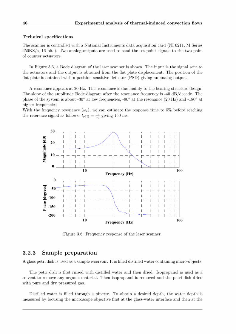
46 Experimental analysis of thermal-induced convection flows
Technical specifications
The scanner is controlled with a National Instruments data acquisition card (NI 6211, M Series250KS/s, 16 bits). Two analog outputs are used to send the set-point signals to the two pairsof counter actuators.
In Figure 3.6, a Bode diagram of the laser scanner is shown. The input is the signal sent tothe actuators and the output is obtained from the flat plate displacement. The position of theflat plate is obtained with a position sensitive detector (PSD) giving an analog output.
A resonance appears at 20 Hz. This resonance is due mainly to the bearing structure design.The slope of the amplitude Bode diagram after the resonance frequency is -40 dB/decade. Thephase of the system is about -30◦ at low frequencies, -90◦ at the resonance (20 Hz) and -180◦ athigher frequencies.With the frequency resonance (ωr), we can estimate the response time to 5% before reachingthe reference signal as follows: tr5% = 3
ωrgiving 150 ms.
Magn
itu
de
[dB
]
Frequency [Hz]
Frequency [Hz]
10 100
10010
0
10
20
30
Ph
ase
[d
egre
es]
-50
0
-100
-150
-200
Figure 3.6: Frequency response of the laser scanner.
3.2.3 Sample preparation
A glass petri dish is used as a sample reservoir. It is filled distilled water containing micro-objects.
The petri dish is first rinsed with distilled water and then dried. Isopropanol is used as asolvent to remove any organic material. Then isopropanol is removed and the petri dish driedwith pure and dry pressured gas.
Distilled water is filled through a pipette. To obtain a desired depth, the water depth ismeasured by focusing the microscope objective first at the glass-water interface and then at the

3.3 Experimental analysis of convection flows 47
water-air interface. The water depth hence sequentially adjusted by adding or removing dropletswith the pipette until getting the working depth.Next, micro-objects are carefully deposited on the water-air interface using tweezers. In orderto immerse objects in the medium, a droplet is removed from the sample with a pipette andthen re-dropped on them.
The microscope objective is focused at the glass-water interface in order to focus the IR laserand to image the micro-objects.
3.3 Experimental analysis of convection flows
In order to characterize convection flows, velocity patterns of glass spherical beads ranging from31 µm up to 270 µm in diameter are measured. Moreover, the effect of the water depth on thedisturbed liquid zone due to the laser spot is presented. These analysis lead to an estimation ofthe fluidic forces acting on the spherical beads.
3.3.1 The disturbed fluidic zone
When heating a thin water layer from below using an IR laser, toroidal-shaped subsurface flowsare generated around the focal point. Localized high-speed flows can then be shaped withinan extent water layer. Micro-objects remaining within this region are dragged toward the focalpoint by the subsurface flows, and dragged away by the surface flows.The IR laser is shot at the middle of a petri dish containing distilled water and hollow glassbeads ranging from 8 up to 12 µm used as tracers. Their densities are close to water density.Figure 3.7 shows a region of convection flows (lighter gray zone) while focusing at the petri dish’ssurface. This region appears when the laser is shot. Beads within this part are radially draggedby the flow toward the center, where the laser is focused. At this point beads are directed towardthe water surface and they start going out of focus. Therefore a darker zone is built up. Thispicture was taken when the convection region reaches its maximum diameter. The water depthis 450 µm and the measured radius is about 2.15 mm.
In Figure 3.8 the variation of the fluidic radius with respect to the water depth is shown.Three different water depths, 150, 300 and 450 µm are compared. The fluidic flow radiusincreases with the water depth. For a depth of 150 µm a radius of about 1.2 mm is obtained;and respectively a radius of 2.15 mm for 450 µm in water depth. Each measurement is repeatedfive times.
In Figure 3.9 an image sequence of a convection cell build-up is depicted. Ten images areshown at 110 ms intervals. Images capture rate is 100 Hz. It was observed that at 20 msparticles laying at the bottom surface starts moving. The time for the convection cell to reachits maximum diameter is about 1 s. At 220 ms, the diameter is already about 70% of itsmaximum value.
3.3.2 Velocity measurements
To proceed with bead velocity measurements, toroidal convection flows are generated by heatinga thin water layer from below using a focused IR laser. A spherical glass bead is placed at adistance from the IR focal point. When the laser is switched on, the fluid starts moving and thebead is dragged toward the laser. The motion of the bead is captured by a high-speed camera

48 Experimental analysis of thermal-induced convection flows
1 mm
laser
focal point
convection
cell
Figure 3.7: Picture of a convection cell within 450 µm of water depth. At the center, theaccumulation of beads show the laser position. Hollow glass beads in the range of 8 up to 12 µmare used as tracers.

3.3 Experimental analysis of convection flows 49
150 300 4500
0.5
1
1.5
2
2.5
water depth [µm]
flu
idic
ra
diu
s [m
m]
Figure 3.8: Fluidic flow radius vs different water depths. The radius increases with the waterdepth. Error bars are taken over ten measurements.
1 mm
Figure 3.9: Convection cell build-up while irradiating with an IR laser. The laser position isat the center of the convection cell. Every picture is shown at 110 ms of intervals. The waterdepth is 150 µm and particles used as tracers are hollow glass beads of 8-12 µm in diameter.

50 Experimental analysis of thermal-induced convection flows
at a frame rate of 80 Hz. The sequence is analyzed by image processing to compute the beadposition in respect to the laser focal point. The velocity profile is then obtained by the differencebetween two successive bead positions multiplied by the frame rate.
The velocity of different bead sizes within different water depths are investigated. The beadsizes range from 31 µm up to 270 µm. The water depth values are 375, 450, 600 and 750 µm.It should be noted that the beads remaining at the petri dish surface before switching the laseron are laying on the glass-water interface. Each measurement shown is the mean of ten mea-surements.
Figure 3.10 shows an image sequence and associated image processing for bead velocitymeasurements. A glass bead was placed at a specified distance (about 800µm) from the laserfocus. The laser is then switched on in a continuous mode and switched off once the glass beadreaches the laser focal point. When the IR laser was on, the bead moves toward the laser focus(white region in Figure 3.10a) and stops close to the focal point. The glass bead’s displacementis monitored with the high speed CMOS camera at 80 Hz. The images are processed (3.10b)one by one, to determine the distance and velocity field between the bead’s center of mass andthe laser focal point. The velocity is then computed by multiplying the difference between twosuccessive center-of-mass positions and the frame rate.
(a) (b)
Figure 3.10: Image sequences for velocity measurements of a spherical glass bead with 92µmin diameter and within 600µm of water depth. One image every 212.5ms is shown. (3.10a)Sequence taken at 80Hz. (3.10b) Image processing to determine the velocity field between thelaser and bead. The mass center is obtained from the white region for each image, and thenthe distance between two successive mas center is computed and multiplied by the frame rate.Scale bar 100µm.
Figure 3.11 depicts the radial velocity field of a glass bead of diameter 92 µm, immersed inwater and in contact with the petri dish surface. The zero point of the x axis corresponds tothe focal point of the laser. Marangoni convection depends inversely on the liquid depth: thesmaller this depth, the larger the flow velocity. Three different water depths of 375, 450 and600 µm were investigated.As shown in this Figure, the bead velocity field increases while decreasing the water depth. Thisis due to the increase of the temperature gradient at the water-air interface, as more energy

3.3 Experimental analysis of convection flows 51
Figure 3.11: Velocity of a glass bead with 92µm in diameter vs the radial distance of the beadcenter to the laser focus (origin) with 3 different water depths.
Figure 3.12: Velocity of 3 different glass beads of 92, 62, 31 µm in diameter vs the radial distanceto the laser focus.

52 Experimental analysis of thermal-induced convection flows
from the laser beam reaches this interface: the absorption coefficient, 23.45/cm, leads to a laserpenetration of about 425 µm. An increase in the temperature gradient causes an increase in thevelocity gradient.
It is observed that the bead velocity increases until reaching a maximum, then decreasesas the bead approaches the laser focal point. This is because that at the beginning the beadstarts being dragged by the flows, thus gaining in speed. However, approaching the laser or heatsource, the flows starts going up. It means that the flows change their direction from radial tovertical. Therefore, the bead is dragged by a decreasing radial flow. As a result, the bead stopsin the laser position where the radial flow is null.
Figure 3.13: Velocity of glass beads with 92 and 31 µm in diameter for 600 µm water depth vsthe radial distance to the laser focus. Error bar is calculated over ten measurements.
A comparison between the velocity fields of different bead sizes is depicted in Figure 3.12 for450 µm water depth. It shows that the bead velocity depends on the bead size for a given waterdepth (450 µm). Naturally, the drag force is also larger. A larger bead will also be heavier.However, at this scale surface effects are dominant over inertial effects and the flow has a greatersurface area to push against. For smaller beads, there is a smaller contact surface area withthe flow and they may become totally immersed in the boundary layer, decreasing significantlytheir velocity.
Figure 3.13 shows the velocity profiles for beads of 92 and 31 µm in diameter (the largestand smallest beads used for these measurements) in a water depth of 600 µm. The error baris calculated as the standard deviation over ten measurements. The errors are larger for highervelocities. These errors are due to the bead initial positions with respect to the laser focal point.
Figure 3.14 illustrates the maximum bead velocity for different bead sizes, 31, 45, 62, 71, 79and 92 µm in diameter, in three different water depths 375, 450 and 600 µm, respectively. Noticethat in all cases, the maximum velocity increases while decreasing the water depth. For a givendepth, considering all the different bead sizes, the maximum bead velocity tends to decrease asbead size get smaller. The water depth are increased by 75 µm and then 150 µm from 375 µm,to reach 450 and 600 µm. By taking the maximum peak velocity for 375 µm of water depth as

3.3 Experimental analysis of convection flows 53
reference, a 92-micron bead exhibits a speed decrease of 21% and 54.8% as water depth increasesfrom 375 µm to 450 µm and 600 µm respectively. The velocity decrease is about 2.6 times whenreducing the water depth by a factor of 2 (150 µm).For a 31µm bead the speed decreases were about 16.8% and 42.4%. For a 71 µm bead, thevelocity decrease is about 3 times. From Figure 3.14, one can conclude that if the water depthis increased by a factor of 2, the velocity for a constant bead size decreases between 2.5 to 3times.
Figure 3.14: Peak velocity of glass beads 31, 62, 71, 79, 92µm in diameter respectively for threedifferent water depth of 375, 450, 600µm.
As shown in Figure 3.15, the velocity profile of a thin liquid layer locally heated from belowhas a pair of counter subsurface convection flows. Close to the free surface, flows are directedaway from the heat source, and toward the reservoir surface flows are directed toward the heatsource. Hence, convection flows reverse their direction from the top (top subsurface flow: TSF)toward the bottom (bottom subsurface flow: BSF) at a given depth. At this position, flows arealmost null.
As seen previously, a bead velocity increases with the bead size. It would reach its maximumvelocity if the bead size is exactly the dimension of the BSF depth, as the whole BSF velocityprofile would drag the bead. However, if the bead size is larger than the BSF depth, it is ex-pected that the velocity decreases because of the counter flows in TSF region.
3.3.3 Influence of larger beads
Velocity measurements on a 240 µm in diameter glass bead are presented in Figure 3.16. Alarger bead size is selected to find the decrease of the bead velocity by decreasing the waterdepth. The bead is placed at about 550 µm from the laser focus. The laser is then switched onduring 100 ms. Three different water depths are investigated, 250, 300 and 450 µm.As compared to previous results, the bead velocity increases by decreasing the water depthfrom 450 to 300 µm. Maximum velocity values range from 4.3 mm/s to 6 mm/s. Therefore,the distance covered by the bead increases while decreasing the water depth. For 300 µm the

54 Experimental analysis of thermal-induced convection flows
distance covered is 270 µm and for 450 µm, a distance of 220 µm is measured as the fluid velocityfor a smaller water depth is larger.On the contrary, when the water depth is almost identical to the bead size, the bead velocitydecreases, as in the case of 250 µm water depth and a 240 µm bead. The counter TSF flowacts also on the bead’s top part, diminishing drastically its velocity. In this case, a maximumvelocity of about 1.8 mm/s is found and the distance covered by the bead center of mass isabout 80 µm.
glass substrate
water
microbeads
air
convection flows
IR laser beam
Figure 3.15: Illustration of the fluid velocity profile with respect to microbeads size. Around thefree surface, flows go away from the heat source (IR laser beam), around the reservoir bottomsurface flows are directed toward the laser beam. Keeping the water depth constant, a microbeadcan be dragged either by the bottom subsurface flows or also by the top subsurface flows.
3.3.4 Micro-objects floating on the water-air interface
As the top subsurface flows (TSF) is directed away from the heat source, micro-objects remain-ing at the free surface are repelled from the heat source. However, when the bead size becomeslarger than the TSF depth, the the bottom subsurface (BSF) acts also on the microbead. Hence,for a given floating micro-bead size, it can be dragged toward the heat source, when the influenceof the BSF over the bead become larger than the TSF influence (cf. Figure 3.17).
Figure 3.17 depicts the convection flows velocity profile with respect to a floating microbeadsize. For a constant water depth, a floating microbead can be dragged away from the heat sourceor toward the heat source, depending on its size.
Figure 3.18 shows an image sequence of a floating glass bead in motion. The bead size is180 µm in diameter. Each image is taken at 33.3 ms of intervals. The position of the IR lasershot is represented by the white region. At water depth 450 µm it is observed that the beadgoes away from the laser beam. It means that the TSF are dominant over the BSF, or the bead

3.3 Experimental analysis of convection flows 55
150 200 250 300 350 400 450 500 5500
2
4
6
Radial distance to the laser focus [µm]
Bea
d ve
loci
ty [m
m/s
]Glass bead of 240 µm in diameter
250 µm300 µm450 µm
Figure 3.16: Velocity profile of a 240 µm glass bead for 250, 300 and 450 µm of water depth.The bead is placed at about 550 µm from the laser focal point. The laser is switched on during100 ms.
glass substrate
watermicrobeads
air
convection flows
IR laser beam
Figure 3.17: Illustration of the convection flow profile with respect to floating microbeads in athin water layer. If a microbead bead size is comprised within the top subsurface flows (TSF), thebead is pushed away from the heat source. For a much larger microbead, the bottom subsurface(BSF) flows acts also the bead and this one is dragged toward the laser beam.

56 Experimental analysis of thermal-induced convection flows
is only subject to the TSF.When the water depth is reduced from 450 to 375, 300 and 265 µm, at 300 µm the bead velocityis diminished significantly, meaning that there was no dominance observed between TSF andBSF. At d=265 µm, the bead goes toward the laser beam as observed in Figure 3.18b. In thiscase, the BSF is dominant over the TSF.For a bead of 270 µm in diameter at d=750 µm the bead is pushed away from the laser, at500 µm it remains almost static, and finally at 450 µm is dragged toward the laser beam.
With these localized convection flows, it is hence possible not only to manipulate immersedmicro-object but also floating beads. As observed, it is much more controllable to drag floatingbeads toward the heat source than away from it. In this configuration, the bead is attracted tothe laser remaining close to it. However, this kind of trapping scheme has not been investigatedin this work.
150 µm
laser
(a)
150 µmlaser
(b)
Figure 3.18: Image sequence showing the displacement of a floating glass bead of 180 µm indiameter. The dashed circles illustrate the bead-air interface. The white region is a focused redlaser and indicates the IR laser shot. Every image is shown at intervals of 33.3 ms. (a) Themicrobead goes away from laser beam within 450 µm in water depth. (b) The microbead goestoward the laser bead within 265 µm in water depth.
3.3.5 Estimation of the manipulation force
In the proposed convection flow based manipulation process, the motion of microparts in theliquid is due to the motion of the liquid around which exerts a viscous force on them. This forceis naturally proportional to the velocity difference between the flow and the object, hence islimited by the maximum velocity of the liquid. Thus, the evaluation of the manipulation force

3.3 Experimental analysis of convection flows 57
requires to define the velocity profile of the convection flow.
In order to estimate the fluid velocity profile that drags a spherical beads and supposing thatthe immersed beads remain on the substrate surface, a rolling with sliding model is considered.
It is assumed that the spherical bead and the horizontal plane are rigid and non-deformable
Figure 3.19: Schematic of the forces involved for the estimation of the fluidic forces exerted ona spherical microbead within a liquid medium.
Figure 3.20: Net force computed with the bead center of mass acceleration (cf. Eq. 3.1). Aglass bead of 92 µm in diameter is used within 450 µm in water depth. The acceleration datais taken by deriving twice the bead position.
bodies. The micro-sphere is uniform of mass m and radius R.
The dynamic equations that describe the motion of the bead can be written as:
∑
F = macm, (3.1)
∑
M = Icmα, (3.2)

58 Experimental analysis of thermal-induced convection flows
where acm is the acceleration of the bead center of mass, Icm (2/5mR2 for a sphere) is themoment of inertia about an axis through the center of mass, M is the resultant torque, F is thenet force and α is the angular acceleration. acm is computed from Figure 3.12, by derivation ofthe velocity data with a time step of 1/80 s. The net force F is then calculated multiplying acmby the mass of the bead (see Figure 3.20).Althought it is observed that the bead rolls while moving, only the motion due to the linearacceleration of the bead is considered here as a first approximation. The moment equation isnot analyzed.
Based on these equations, a force analysis on a bead gives the following set of equations (aschematic of this analysis is shown in Figure 3.19). The net force is the sum of the viscous dragforce exerted by the fluid and the friction.
F = Fd − Ff , (3.3)
where Fd is considered the viscous force applied on the bead and Ff is the friction force opposingthe bead motion.As the motion is rolling with sliding, the friction force is a kinematic friction force:
Ff = µkFN , (3.4)
where µk is the coefficient of kinematic friction between the two surfaces and FN is the normalforce exerted on the bead. This latter force is equal to the difference between the bead weightand the Archimedes force FA = ρgVvolb, where ρ is the water density, g is the acceleration ofgravity and Vvolb is the bead volume.Therefore the force equation on the vertical axis is:
FN = mg − FA. (3.5)
The mass of the bead is m = ρbVvolb where ρb is the density of glass (2500 Kg/m3) andVvolb = 4/3πR3.
The coefficient of kinematic friction for a glass-glass relative motion within water medium isµk = 0.2 (Ishibashi et al., 1994).
As the acceleration is measured through velocity, and the mass of the bead is known, theviscous force applied on the object can be written as:
Fd = macm + Ff (3.6)
Fd is due to the relative velocity between the spherical bead and the convection flow:
Fd = A(vf − vb), (3.7)
where A is the drag coefficient in low Reynolds Stokes flow for a spherical shape: A = 6πµR,vf is the velocity of the fluid and vb is the velocity of the bead (cf. Figure 3.12).
Hence, using equations 3.6 and 3.7 vf can be expressed as:
vf =macm + Ff +Avb
A(3.8)
These results are reported in Figures 3.21 and 3.22 for the force due to flows speed and theestimated speed of flows respectively.
The maximum force that can be exerted on the bead is naturally located at the maximumflow velocity point. It appears that with convection flows, significant forces can be exerted. Forinstance, these forces are much larger than optical tweezers forces: 5 nN vs tens of pN.

3.3 Experimental analysis of convection flows 59
Figure 3.21: Estimation of the force that the flows exerted on a 92µm-sized glass according toEq. 3.8.
Figure 3.22: Estimation of the flows velocity distribution that drags a 92µm-sized glass immersedin a water depth of 450 µm according to Eq. 3.8.

60 Experimental analysis of thermal-induced convection flows
3.4 Conclusions
An experimental set-up have been developed in order to generate thermocapillary convectionflows which are used to drag micro-parts. A focused 1480 nm IR laser was used to locally heata thin liquid layer of distilled water and to generate localized convection flow.
This permitted manipulation without the need for patterned or microfabricated substrates.A simple petri dish was filled with liquid water to a predetermined depth.Velocity measurements of glass beads (ranging from 31 to 92µm in diameter) were performedwith a high speed CMOS camera. Results showed that the largest glass bead (92µm in diame-ter) was dragged at about 5.5 mm/s in 375µm water depth. It appeared that the bead velocitydepends on the bead size. The larger the size, the larger the velocity, because the flow veloc-ity profile on its surface is larger. For smaller beads, the velocity profile decreases due to theboundary layer at the substrate-water interface.The bead velocities also depend on water depth; the smaller the water depth, the higher thebead velocity. The manipulation velocity could be controlled to handle particles by adjustingthe water depth.
Also, a force model is proposed in order to estimate the exerted forces by the flows on thebeads. It appears that it is possible to exert forces approximatly 100 larger than optical tweezers.

Chapter 4
Toward a fully automated
vision-based opto-fluidic system for
non-contact micromanipulation
There is a computer disease that anybody who works with computers knowsabout. It’s a very serious disease and it interferes completely with the work. Thetrouble with computers is that you ’play’ with them!
Richard P. Feynman
The growing development and production of microsystems in both the industrial and researchfield requires versatile and high-autonomous micromanipulation systems. The increase in thediversification, therefore in complexity, of these systems such as MEMS, NEMS, MOEMS andrecently bioMEMS, needs the use of different and several microfabrication processes to engineermicrocomponents. And these components, made of different geometries, materials and proper-ties, have to be assemble to form microsystems for a wide variety of applications. Due to thepotential market of these micro and nano devices, industries need to improve their throughput.Indeed, the micromanipulation and assembly of these components rely on operators limitinglarge production. However, with autonomous micromanipulation and assembly systems high-throughput and cost-effective devices could be carried out. Moreover, more precise and reliablemanipulation and assembly could be achieved.
This field is rapidly progressing as autonomous micromanipulation is of great interest nowa-days. Several research groups are working on micromanipulation systems. Most of worksare based on mechanical or contact micromanipulation mode (Dionnet et al., 2004, Sitti &Hashimoto, 2000, Probst et al., 2009). However, contact micromanipulation is a slow processthat does not allow parallel manipulation capabilities due to the limited displacement speed ofthe microtools (tens of microns per second).
Among non-contact micromanipulation systems, optical tweezers have reached a high degreeof autonomy (Tanaka et al., 2008, Arai et al., 2004). Nevertheless, this technique is limited toobjects up to tens of microns in size.

62
Toward a fully automated vision-based opto-fluidic system for non-contact
micromanipulation
Autonomous micromanipulation is also of interest in biology and the manipulation of livingcells such as bacterias and embryos (Yu & Nelson, 2001).
In the previous chapter, it has been demonstrated that convection flows induced by a laser canbe successfully used to displace microscopic particles in a liquid medium. In order to automatethis novel manipulation method, it is necessary to implement a closed loop feedback mechanism.The chosen feedback is vision through optical microscope. Several image processing methodsare first evaluated in order to implement the most adapted to the system. Then the calibrationof the micromanipulation system is detailed, followed by the operation modes developed.
4.1 Vision feedback for micromanipulation
Vision feedback is widely used for robotic manipulation, especially in the macroscale where cam-eras can be easily used as optical sensors.In the microscale the use of vision feedback is attractive because of the lack of alternative sensingsystems. Optical microscopes are coupled to a camera to provide a visual feedback to the useror a position information to microrobotic systems.In nanomanipulation, due to the limited optical resolution, other instruments are used for po-sition feedback such as a Scanning Electron Microscope (SEM). Even hybrid systems (opticalmicroscope-SEM) can be used for a 3D micro/nanomanipulation (Jahnisch & Fatikow, 2007).
This section addresses different methods in vision feedback using image processing for mi-croscopic applications in order to select the most adapted to our system. Image processing willallow to calibrate the system and to track the moving particles. For calibration, the detectionof the IR laser position on the sample is needed. For tracking, a robust and fast method isrequired.
4.1.1 Optical flow
This method is used to estimate the relative motion of features in an image at time t withrespect to an image at time t+δt. It is based on the smooth intensity variation of these featuresbetween two successive images, I(x, y, t) and I(x + δx, y + δy, t + δt). Moreover, the featuremotion between two images is assumed to be very small in order to obtain:
δI
δxVx +
δI
δyVy = −
I
t,
where Vx and Vy are the optical flow velocity of I(x, y, t). In microscopic environments wherethe illumination and environment are well controlled, this method is proved to be robust.As an example, (Yu & Nelson, 2002) uses an optical flow tracking algorithm for visual servoing ofa microrobotics system. A tip of an injection pipette is tracked to inject foreign genetic materialinto cells.
4.1.2 Image segmentation
Segmentation is widely used from microscopic detection to vision-based robot control. It isan image process that partitions an image into homogeneous non-intersected features in whichconnected pixels are labeled.
There are different techniques to implement image segmentation such as histogram thresh-olding and edge detection (other approach can be used (Pal & Pal, 1993)).

4.1 Vision feedback for micromanipulation 63
Histogram thresholding is one of the simple and popular image segmentation techniques where agray level information is used. Thresholding techniques can be classified as global thresholdingand local thresholding. When only a threshold is used for the whole image, it is global thresh-olding. When an image is partitioned into several subregions, several thresholds are necessaryfor each region, it is local thresholding or also called adaptive thresholding. In case where animage is partitioned into two regions, black and white, it is called bilevel thresholding.Edge detection can also be used for image segmentation. Features are obtained by detecting astrong gray level gradient at the object’s borders. Methods such as Sobel gradient and Laplacianoperator are generally used. The Sobel’s operator is a first differential operator with a very goodimmunity to noise. On the other hand, the Laplacian operator is a second differential operatorand responds strongly to corners, lines, and isolated points. However, it is heavily influenced bynoisy images.
(Chen et al., 2006) showed the use of advanced segmentation techniques such as the Water-shed segmentation to detect and track individual cells in a living cell population (cf. Figure 4.1).
Figure 4.1: Image segmentation of cells (Chen et al., 2006). It shows the separation of featureswith different advanced segmentation techniques
4.1.3 Hough transform
This method is most commonly used to detect lines and circles. It is a robust method whenworking under noisy conditions such as optical microscopes. Hough transform involves trans-forming each of a figure points in a parametric representation within a parametric space. Forexample, a line is represented by a point in its parametric space. In order to find a line in apicture, every point is transformed in its parametric representation. However, an infinity of linescan passes through a point, a family of lines. This family is represented by a sinusoidal curve inthe parameter space. Hence two points have two sinusoidal representation, and the intersectionpoint of these curves is the line passing through both points in the picture.The Hough transformation has a generalized form, any shape of feature can be detected. How-ever, the number of parameters increases with the complexity of the feature shape. Therefore,this method becomes time-consuming in computer vision.This method was used by (Pawashe & Sitti, 2006 and Tanaka et al., 2008) to detect micro-objects.(Pawashe & Sitti, 2006) performed automatic micromanipulation of sphere by a mechanical tech-nique with vision feedback. (Tanaka et al., 2008) used also image processing to automaticallyhandle non-spherical micro-objects using optical tweezers.
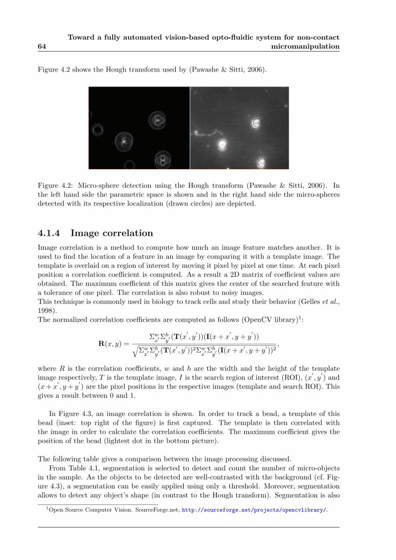
64
Toward a fully automated vision-based opto-fluidic system for non-contact
micromanipulation
Figure 4.2 shows the Hough transform used by (Pawashe & Sitti, 2006).
Figure 4.2: Micro-sphere detection using the Hough transform (Pawashe & Sitti, 2006). Inthe left hand side the parametric space is shown and in the right hand side the micro-spheresdetected with its respective localization (drawn circles) are depicted.
4.1.4 Image correlation
Image correlation is a method to compute how much an image feature matches another. It isused to find the location of a feature in an image by comparing it with a template image. Thetemplate is overlaid on a region of interest by moving it pixel by pixel at one time. At each pixelposition a correlation coefficient is computed. As a result a 2D matrix of coefficient values areobtained. The maximum coefficient of this matrix gives the center of the searched feature witha tolerance of one pixel. The correlation is also robust to noisy images.This technique is commonly used in biology to track cells and study their behavior (Gelles et al.,1998).The normalized correlation coefficients are computed as follows (OpenCV library)1:
R(x, y) =Σwx′Σhy′ (T(x
′
, y′
))(I(x+ x′
, y + y′
))√
Σwx′
Σhy′
(T(x′ , y′))2Σwx′
Σhy′
(I(x+ x′ , y + y′))2,
where R is the correlation coefficients, w and h are the width and the height of the templateimage respectively, T is the template image, I is the search region of interest (ROI), (x
′
, y′
) and(x+ x
′
, y+ y′
) are the pixel positions in the respective images (template and search ROI). Thisgives a result between 0 and 1.
In Figure 4.3, an image correlation is shown. In order to track a bead, a template of thisbead (inset: top right of the figure) is first captured. The template is then correlated withthe image in order to calculate the correlation coefficients. The maximum coefficient gives theposition of the bead (lightest dot in the bottom picture).
The following table gives a comparison between the image processing discussed.
From Table 4.1, segmentation is selected to detect and count the number of micro-objectsin the sample. As the objects to be detected are well-contrasted with the background (cf. Fig-ure 4.3), a segmentation can be easily applied using only a threshold. Moreover, segmentationallows to detect any object’s shape (in contrast to the Hough transform). Segmentation is also
1Open Source Computer Vision. SourceForge.net, http://sourceforge.net/projects/opencvlibrary/.

4.2 System calibration 65
Figure 4.3: Images of a correlation method applied to track a glass spherical bead. The bottomimage is the result of the correlation method applied to the top image. In the top right cornerthe template is shown.
Table 4.1: Comparisons of image processing methods
Method Robustness time to process feature detection
Optical flow low no so fast badSegmentation low fast goodHough transform high no so fast good for lines and circlesCorrelation high fast if ROI very small good. Template required
used to calibrate the system, where the laser position is required. This process is explained inthe next section.For the bead tracking process, correlation is preferred because it is robust, fast for small ROIsand accurate.
4.2 System calibration
The micromanipulation system has to be calibrated due to distortions introduced by the laser-scanner, in order to have a precise control on the beads positions.This means that the laser, displaced by the tip/tilt scanner on the sample, is not projectedexactly on the desired position. For instance, if a square reference is given to the scanner, onthe sample this desired square trajectory of the laser is curved due to the scanner’s distortions(see Figure 4.5). These distortions are explained in details in (Hafez, 2000).
To correct these distortions a third degree polynomial approximation is used in order tohave:
xcorrected = axx+ bxy + cxx2 + dxxy + exy
2 + fxx2y + gxx
3 + hxy2x (4.1a)
ycorrected = ayx+ byy + cyx2 + dyxy + eyy
2 + fyx2y + gyx
3 + hyy2x (4.1b)
where xcorrected and ycorrected are the corrected positions to be sent to the scanner command, xand y are the desired positions of the laser on the sample. To calculate the coefficients, at leasteight positions values of x and y are required to obtain a system of eight equations and eightunknowns. The index 1 to 8 represent eight measurements of the laser positions. The resulting

66
Toward a fully automated vision-based opto-fluidic system for non-contact
micromanipulation
equation system is as follows:
x1corrected...
x8corrected
︸ ︷︷ ︸
X
=
x1 y1 x21 x1y1 y2
1 x21y1 x3
1 y21x1
......
x8 y8 x28 x8y8 y2
8 x28y8 x3
8 y28x8
︸ ︷︷ ︸
P
×
ax...hx
︸ ︷︷ ︸
C
, (4.2)
As C is the unknown, the inverse of P is calculated to obtain:
P−1X = C (4.3)
In Figure 4.4 the process where X, P and C intervene is shown.In order to solve this system, a square reference composed of eight positions values is used for X(see the square marks in Figure 4.5). The values of P , the eight laser positions that correspondto the command reference X, are captured by a camera and calculated by image segmentation(see Figure 4.6). The IR laser causes a circular shadow in the water layer, this shadow is detectedwith image background subtraction. It means that, an image of the sample without laser is firstcaptured with a camera. The laser is then shot into its respective reference position in orderto capture a second image containing the IR laser’s shadow. By subtracting both images, onlythe IR shadow is obtained (cf. Figure 4.6a). The center of the shadow, center of the IR laser, iscomputed with image segmentation using thresholding (see Figure 4.6b).P is then calculated with the eight laser’s positions, X is the command reference and C iscalculated according to Eq. 4.3.C is used to correct the desired positions and compute a new command reference for the scanner.For instance, if a line trajectory of the laser is desired (square marks in Figure 4.7), a curvereference trajectory has to be sent to the scanner according to Eq. 4.1 (circle marks in Figure 4.7).
Figure 4.4: Block schemes illustrating the calibration process where the polynomial approxima-tion is used.
A flow chart for the calibration process is shown in Figure 4.8. Eight reference positions aresent to the laser, at each position the laser is detected using image processing and its center iscalculated. This is performed consecutively for the eight reference positions. Once the laser’positions computed, the coefficients for the polynomial approximation are calculated.
The calibration process allows to have a precise control on the bead’s positions, thus themanipulation system is implemented in two operation modes: manual and automatic.

4.2 System calibration 67
0 100 200 300 400 5000
100
200
300
400
500
x image frame [pixels]
y im
ag
e f
ram
e [
pix
els
]obtained ref.
expected ref.
Figure 4.5: Simulation of geometrical distortions. If a square reference is sent to the laserscanner, a curve quadrilateral is obtained on the sample due to the scanner’s distortions.
(a) (b)
Figure 4.6: Superposition of eight images containing the reference laser positions on the sample.(a) Background image subtraction to detect the IR laser positions. (b) Image binarization ofeach point found after background subtraction. Then morphological operations are used toimprove the image quality. Computation of the objects’ center of mass using OpenCV.

68
Toward a fully automated vision-based opto-fluidic system for non-contact
micromanipulation
0 100 200 300 400 5000
100
200
300
400
500
x image frame [pixels]
y im
ag
e f
ram
e [
pix
els
]desired ref.
corrected ref.
Figure 4.7: The calibration process allows to obtain a line reference on the sample (square marks)by sending a curve trajectory (circle marks) to the laser scanner. This curve is determined by apolynomial approximation.
Figure 4.8: Flow chart illustrating the system calibration process.

4.3 Micromanipulation: Operation modes 69
4.3 Micromanipulation: Operation modes
Two operation modes have been implemented with a C++ program:
1. A manual operation mode, in order to handle different micro-parts such as spherical beads,silicon cubes solder beads and capacitors to move them in desired positions. In this mode,the user, through a computer mouse, addresses the laser at a target position within theimage frame to drag the micro-objects toward this position in the workspace.
2. An automatic operation mode, in order to handle multiple beads autonomously. In thiscase, a reference position value is introduced in the program. The laser is then automat-ically addressed to a determined position close to the bead to drag it toward their finalpositions.
4.3.1 Manual operation mode
A manual micromanipulation mode is first implemented, in which the user can drag differenttypes of beads such as glass beads, silicon microcubes, solder beads and capacitors.The user controls the laser-scanner displacement by moving a computer mouse onto the videoframe displayed on a Graphical User Interface (GUI). The user can shoot the IR laser at adesired position by pressing the mouse’s left button. The laser exposure time is a parameterthat can be changed in the computer program.The user has to manage to shoot the laser at a distance from the micro-object in order to dragit. As seen in chapter 3, the beads go faster when the laser is irradiated at a predetermineddistance from the beads. The bead velocity depends on this distance and the exposure time.The only feedback that the user have is the video frame displayed on the computer screen. Theuser has to correct the laser position with respect to the micro-part position by looking at thecomputer screen.
Figure 4.9 illustrates the overview of the manual operation mode. The user controls the laserposition and laser exposure time with the computer mouse. When a mouse click is performed,the mouse position in pixels is introduced in the program. The laser-scanner and IR laser arethen actuated and pointed at the mouse position. The user has to see the bead position and todisplace the IR laser with respect to the bead in order to drag it close to the desired positiondestination.
This manipulation mode is used to handle spherical beads and larger and heavier non-spherical parts. In the case of heavier micro-parts, acoustic vibrations are applied to the sub-strate in order to break the adhesion forces between the parts and the substrate.
Handling of spherical beads
The handling of spherical beads is shown in Figure 4.10. In the first sequence of pictures, theseparation of three beads previously in contact and placing them at different positions is per-formed. The bead sizes lie between 75 up to 85 µm in diameter. They are immersed in distilleda water depth of 300 µm. Pictures are taken every 8 seconds. The bead speeds are in the rangeof 1 to 3 mm/s. The red dot is the position of the IR laser. Manipulation is simply made bymoving the laser focal point with the mouse and by clicking to apply a 20 to 100 ms of the IRlaser (cf. Figure 4.10a). The user has to point the laser at a suitable position with respect tothe beads in order to handle them with a desired speed. In addition, the user has to deal with

70
Toward a fully automated vision-based opto-fluidic system for non-contact
micromanipulation
Figure 4.9: Representation scheme of the manual operation mode.
the displacements of the beads at the same time for one laser shot.
The manipulation of beads by scanning the laser in a circular pattern was successfully per-formed. The particles are in this case trapped in the middle of the circle. This result is interestingbecause the particle stays away from the laser irradiation. Also, we observed that the micro-objects trapped this way tend to rotate at a slow speed. The direction of the rotation can becontrolled by the direction of the laser rotation. This feature may be use for precise positioningeither in translation or rotation. Figure 4.10b shows three beads, ranging from 75 to 85 µm indiameter, trapped in the center of a circular laser pattern. A circular pattern is projected onthe working surface to trap the objects. The objects remain in the center due to the radial flowsacting in them.Parallel manipulation of beads was also demonstrated using a linear scanning of the laser. Inthis case the beads follow the laser line in an aligned formation.
Handling of non-spherical micro-parts
Different micropart shapes can be also dragged. Figure 4.12a shows the drag of a silicon micro-cube of 100 µm in side. It is immersed in a PBS solution of 400 µm in depth. The white dotshows the laser position. A speed of 800 µm/s can be reached. Even if the micro-cube has amuch larger surface of contact with the substrate and it does not roll, it can be dragged easilyat a reasonably high-speed.In Figure 4.12b, silicon parts of about 200 µm of maximum size are dragged. They are large
particles with a non-defined geometrical shape. They are also very thin, about 20 to 30 µm inthickness. In this case, the current affecting the object is quite low because of the boundarylayer of the liquid flow. However, they are quite easily manipulated. They are actually trappedin the recirculation zone spinning at the speed of the flows. Figure 4.12b shows a task consistingof bringing all the parts together. Total manipulation time is 20 seconds. The water depth is300 µm.

4.3 Micromanipulation: Operation modes 71
(a)
(b)
Figure 4.10: Pictures depicting the manipulation of beads. (a) Separation of three beads of 75to 85 µm in diameter. The red dot is the laser position. b) Trapping of micro-spheres inside alaser circular pattern. Glass beads of 75 to 85 µm in diameter.
(a)
PZT transducer
petri dish
water layer
(b)
Figure 4.11: Annular PZT piezo-transducer is glued on a petri dish. It engenders acousticvibrations to push the micro-parts up from the substrate. (a) View of the petri dish bottomsurface. (b) Side view of petri dish and transducer.

72
Toward a fully automated vision-based opto-fluidic system for non-contact
micromanipulation
The strong dynamics of these flows allow to drag much larger and heavier microparts. Someexamples are solder beads and microcapacitors. However, for these cases, an annular PZT trans-ducer is used to engender acoustic vibrations in the substrate in order to reduce the adhesionforces. This transducer is glued on the petri dish substrate as shown in Figure 4.11.Figure 4.13a depicts the handling of a lead-tin solder bead of about 200 µm in diameter. Thisbead has not a spherical shape, increasing significantly the contact area with the substrate. Inthis case, the flows are not able to drag the solder bead because of the adhesion forces with thesubstrate. To drag this object, acoustic waves are used to reduce the adhesion forces in sucha way that the solder bead is pushed up from the substrate due to acoustic vibrations. Themanipulation is slow, each of the pictures are shown at an interval of 1.6 s.
Figure 4.13b shows the manipulation of a micro-capacitor within 300 µm in water depth. Itsdimensions are 400 × 200 × 50 µm3. To drag this capacitor, the same PZT transducer is used.The transducer is actuated with a swept back and forth signal from 20 kHz to 150 kHz in 50 mswith an amplitude of 5 V peak-to-peak.The measured manipulation speed is between 20 to 50 µm/s. Each image is shown at an intervalof 4 s.
(a)
(b)
Figure 4.12: Manipulation of non-spherical parts. (a) Silicon cubes of 100 µm in size are dragged.(b) Silicon parts of 200 µm as maximum side are being grouped. The white dot is the laserposition.
The manual operation mode does not allow to handle multiple micro-beads in a fast andprecise manner. On the other hand, an automatic operation mode has been implemented toallow a fast and accurate multiple bead manipulation.

4.3 Micromanipulation: Operation modes 73
(a)
(b)
Figure 4.13: Pictures depicting the manipulation of large and heavy micro-parts. (a) Lead-tin solder bead of 200 µm in diameter is dragged. (b) Manipulation of a capacitor of400 × 200 × 50 µm3 in size. A PZT transducer is used to reduce the adhesions forces with theglass substrate.
4.3.2 Automatic operation mode
Automatic systems for micromanipulation are of great interest in the microtechnology and bi-ology industry or in the research field. It can provide precision, accuracy, massive manipulationand therefore cost-effective production. It can also reduce significantly the time-consuming pro-cess of manual operation modes. Even in the research laboratories it is of great interest tobe equipped with automatic manipulation to test or asses several micro-processes in a more re-duced time such as self-assembly, mixing chemical components, gathering or sorting micro-parts.
In this section, the automation of the micromanipulation system is presented. This is possibledue to the predictable convection flows behavior described in chapter 3 and the negligible inertialeffects.As an example of automatic manipulation, the handling of two glass spherical beads rangingfrom 30 to 90 µm in diameter are reported. Additionally, with the algorithm discussed below,spherical beads up to 300 µm can be automatically manipulated.
Algorithm for automation
An algorithm for automatic operation mode has been developed based on a visual servoing, inwhich the beads are tracked till their final position. The flow chart explaining this algorithm isshown in Figure 4.14. The control algorithm used is as follows:
1. Initialization: Detection of spherical beads using segmentation within an image frame of500 × 500 pixels in size.
2. Image templates of beads are taken and search region of interest (ROI) are located at thebead’s center of mass.

74
Toward a fully automated vision-based opto-fluidic system for non-contact
micromanipulation
3. Reference goal positions are introduced by an user through a computer mouse or specifiedin the program.
4. Close-loop starts: Image correlation starts to the tracking process.
5. The line passing through the bead center of mass position and goal position is computed.
6. Laser-scanner is positioned at a predefined distance d from the bead and the IR laser isshot during an exposure time te. The laser position is located at a distance d that belongsto the precomputed line.
7. The ROI position is updated to the present bead position.
8. The bead is placed at the goal position, the laser-scanner is then positioned at its initialposition. End of process.
The algorithm tests if the bead reaches the goal position, otherwise it continues to the bead’scenter of mass calculation. The IR laser is then shot at a distance d belonging to the line passingthrough the bead and the goal position. The calculation of the bead position is tested. If thebead moves too fast and goes out of the search ROI, the process restarts for detecting the beadlocation.
Program implementation
The automatic mode is implemented using the C++ language in a windows operating system.A multithreaded program was necessary to perform the tracking process, the IR laser shot witha determined exposure time and the GUI display in an independent manner. A serial programblocks these processes while one of them is performed.To implement a multithreaded program in C++, OpenMP2 application programming interface(API) was used. It is an open source library not difficult to be implemented.
Figure 4.15 shows the threads used in the program. Thread1: Image acquisition and GUIdisplay; Thread2: image processing; and Thread3: DAQ NICard, command for laser-scannerand IR laser shot. These threads communicate each other through shared variables. As thethreads are asynchronous, these resources must be protected to avoid their overwriting whilecommunicating, otherwise it can cause wrong calculations.
Tracking method and position feedback
The beads have to be tracked in order to know their position at all times. Their positionsprovide to the system the feedback to know where the laser has to be addressed and if the beadshave reached the desired destination.Image correlation is used to track the beads. Its computing time depends on the ROI size. AROI size of 100 × 100 pixel is used and the time to find a bead (10 to 20 pixels in diameter)within this size is about 2 ms.
Figure 4.16 illustrates how the tracking method works. After detection of bead by segmen-tation, the templates are captured and the ROIs are positioned at the beads’ center of mass.Once the correlation is performed in the whole ROI, the bead position is obtained. A line pathis then calculated between the bead and goal positions. The laser is shot a distance d from the
2OpenMP: Open Multi-Processing API. http://openmp.org

4.3 Micromanipulation: Operation modes 75
Figure 4.14: Flow chart illustrating the control algorithm used for automation.

76
Toward a fully automated vision-based opto-fluidic system for non-contact
micromanipulation
Master thread
Image acquisition
&
GUI display
Image processing
correlation method
Laser-scanner
&
IR laser
NIcard
Close program
shared
variables
shared
variables
I I PP1 10 0
Figure 4.15: Block diagram of the implemented multithreaded program. The main program isdivided into three independent programs which communicates between each other with sharedand protected variables. I0,1 and P0,1 are images and position shared variables.
bead. The bead is displaced by the laser shot. The correlation is performed in order to computethe new bead position. Once the bead position is computed, the ROI updates its location inorder to have the present bead position at the ROI’s center. For a new bead position, the linepath is recalculated to address the IR in this line.For each iteration, the distance between the bead and the goal position is compared to a desiredaccuracy distance introduced in the program. When the bead-goal distance is smaller than theaccuracy distance, the process ends. The highest accuracy that the system can achieve is onepixel, which is the position error given by the image correlation process. In the micromanipula-tion system, one pixel correspond to 5 µm.The time to achieve the displacement of a bead in a close loop is given by the sum of: thelaser exposure time (50-90 ms) and the scanner response time (125 ms) that gives 215 ms. Thecorrelation time (2 ms) is not taken into account because the image correlation is performed ina parallel thread.
Figure 4.16: Representation scheme of the tracking method using image correlation. The laseris shot to drag the bead, the bead moves and the ROI updates its position to find the bead.Once the bead position is computed, the laser is shot.

4.3 Micromanipulation: Operation modes 77
Experimental validation
First experiments are aimed to validate the full automation of this novel non-contact manipu-lation technique. The automatic manipulation of two beads is depicted in Figure 4.17. Thesebeads are 50 and 85 µm in diameter respectively. The water depth is 450 µmFirstly, the beads are located by the user and contained in an image frame of 500 × 500 pixels(Figure 4.17(a)). One pixel corresponds to 5 µm in the workspace. Then the detection process isactivated by the user on the GUI. A detection filter is also implemented to avoid the detection ofimpurities or beads smaller than 30 µm and larger than 150 µm in diameter. These parameterscan be changed in the program.Once the beads are detected, the user introduces the goal positions or destinations by clickingwith a computer mouse on the video displayed (Figure 4.17(b)). The goal positions are shownby a black circle of 50 µm in radius. This dimension also represents the positioning tolerance.That means when the bead’s center of mass is located at a distance smaller the 50 µm from thegoal position, the automatic process stops. This tolerance can be changed in the program.After the introduction of the goal positions, the laser is shot at a distance of 450 µm from eachbead during 90 ms of exposure time (Figure 4.17(c)). The laser position is switched from onebead to the other, thus each bead is moved of one step after the other (Figure 4.17(c-h)). Thisstrategy is implemented due to the radial shape of flows. That means for one laser shot all beadsgo toward the laser if they are close enough.Due to the different distant destinations, one of the two beads arrives to its goal position faster(cf. Figure 4.17(g)). As a result, the laser will focus on the remaining bead till it reaches itsdestination. When the two beads are in their respective goal positions the automatic processstops.The pictures in Figure 4.17(b-h) are shown at an interval of 1 s, taking a time of 6 s, since theuser introduces the goal positions, for both beads to arrive to their destinations.
Limitations of the implemented control algorithm
We demonstrated the automation of this method by implementing a simple position feedback,in which the computed error (distance between the bead and goal position) is compared to thetolerance position without regulation. A regulator can be implemented to improve the perfor-mances of the system, it can increase the speed and accuracy of the automatic process. Forinstance, in our program the distance at which the laser is shot is not variable as well as theexposure time. If this parameters are varied with respect to the position error, the bead couldmove faster when it is far from the goal position and slower when it is close to it. In this way,an accuracy of 1 pixel can be reached in a shorter time. One pixel is the error due to the imagecorrelation.
The main drawback of this method for a multiple bead manipulation is the cross-talk en-gendered due to the radial symmetry of convection flows with respect to the heat source. Theimplemented control algorithm does not take into account this cross-talk. A more sophisticatedalgorithm has to be implemented with a suitable regulator.
Apart from the control algorithm, to better address the cross-talk a faster laser-scanner isrequired. Thus the laser can switch from one bead to another much faster or to produce dedi-cated patterns almost in parallel in order to reduce the cross-talk. The laser-scanner used has aresponse time of about 125 ms.

78
Toward a fully automated vision-based opto-fluidic system for non-contact
micromanipulation
Figure 4.17: Image sequence depicting the automatic manipulation of two beads. (a) The beadpositions are detected by the program. (b) The user introduces the respective goal positionswith a computer mouse by only clicking on the image frame. (c-h) The IR laser is shot byswitching from one bead to the other till the beads arrive to destination. The pictures areshown at intervals of 1 s. Scale bar of 200 µm

4.4 Conclusions 79
4.4 Conclusions
In this chapter a first fully automated non-contact fluidic-based micromanipulation system us-ing visual servoing is presented. Immersed spherical beads ranging from 30 up to 250 µm indiameter can be handled manually and autonomously.The automatic manipulation of two spherical beads is successfully achieved and presented. Alaser-scanner device is used to address an IR laser to a specified position with respect to thebeads and their destinations. The IR laser generates localized convection flows close to thebeads, these flows are used to drag the beads to their destinations.In addition, a manual operation mode is proposed. It allows an user to handle micro-parts byonly clicking with a computer mouse on a image frame displayed on a GUI.
The operation modes developed show the feasibility of handling micro-parts within a liquidmedium. This is of great interest for the fabrication of microdevices, self-assembly or produc-tion with batch processes in the mesoscale. Moreover, our system can be extended to handlebiological cells either in manual or automatic operation modes.
The main drawbacks of this method for a parallel manipulation of single beads, is the cross-talk engendered by the flows. In order to reduce that, a better control algorithm has to bestudied and developed. Moreover, a better control algorithm will allow to enhance greatly theperformance of the method proposed in terms of rapidity, accuracy and number of beads to behandled.Future work will deal with the study of better control and image processing algorithms formultiple beads and non-spherical micro-objects manipulation in an autonomous manner.

80
Toward a fully automated vision-based opto-fluidic system for non-contact
micromanipulation

Conclusions and Perspectives
In this work, a novel contactless micromanipulation technique in fluid medium is developed.Handling micro-parts in the 1 - 100 µm range is an actual challenge for the industrialization ofnew products based on opto-electro-mechanical components, namely MEMS, OLEDs etc. Allthis components are fabricated from bulk on silicon or similar wafers and the production ofcomplex systems requires reliable assembly process.The manipulation technique proposed here is based on the use of thermal induced convectionflows in liquid. The Marangoni effect is a torus shaped flow generated around a local heat sourcein a fluid. The micromanipulation setup designed and constructed in this work generates control-lably these Marangoni convection flows using a single laser beam. A full closed loop operation ispossible thanks to implemented high frequency vision feedback and image treatment. The highdynamic and controllability of the system makes it suitable for massive parallel manipulationand assembly.
In the first chapter, an overview of different micromanipulation methods is given with acomparison of contact and non-contact techniques. These analysis points some advantages ofcontactless techniques, especially when the size and the shape of the objects may vary. Ad-ditionally, contactless methods in liquid allow to minimize the effects of adhesion phenomena,which are the most dominant forces at this scale.Among the liquid convection phenomena, Marangoni effect stands out because of its ability togenerate locally high-speed flows. The strength of these flows and their spatial distributionare enough to drag several micro-parts in parallel. Moreover, as this phenomenon is based onsurface forces (proportional to L), it is more suitable for miniaturisation than free convectionwhich is based on body forces (proportional to L3). Their theoretical and experimental analysisis presented in chapter 2. This analysis shows that this method can be implemented by usinga single laser beam as a heat source. The main advantage advantage of using a laser is that itcan be focused in a very small surface, thus obtaining a very localized convection flows.Additionally, different fluidic flow patterns can be easily performed only by scanning the laserbeam on the sample.
The third chapter describes the experimental setup designed and constructed for Marangoni-effect based fluid micromanipulation. The system is composed of an optical microscope, a scan-ner holding a mirror to address the laser at any point on the manipulation area and a fastcamera based vision system. This system is then characterized in its technical specificities andis used to define physical parameters influencing the Marangoni effect, such as the water depth,object shapes and dimensions the laser power.
The fourth chapter takes the robotic implementation one step further. Based on the cal-

82 Conclusions and Perspectives
ibration physical and technical specificities of the manipulation system, a full automation isimplemented. The control loop is closed using vision feedback. In this purpose, several imagetreatment techniques are investigated in order to implement a high speed feedback loop. Imagecorrelation is used to track the beads on real time. This method is robust to noise and fastenough, allowing to compute the positions of several beads for multiple beads manipulation.Two operation modes are implemented. The first one is the manual operation where the usercontrols directly the laser focal point’s position. The second one is an automatic mode. A fullautomation algorithm is implemented using complete closed-loop vision servoing. The user justpoints the target position and the system drags the object at that desired location. This mode isalso experimentally validated in a multiple manipulation scenarii. In this experiments, the userdefines 2 target positions for two beads and the system moves them to these desired locationswithout further user interaction.
The developed techniques show the feasibility of parallel handling micro-parts within a liq-uid medium using convection flows. This is of great interest for the fabrication of microdevices,self-assembly or production with batch processes in the mesoscale. Moreover, our system canbe extended to handle biological cells either in manual or automatic operation mode.This work opens several perspectives, through a more reliable analysis of the fluidic convectionor by increasing the technical capabilities of the scanner and the vision system, in order to beable to address larger populations of microparts.

Bibliography
Abidin, Z. Z., & Markx, G. H. 2005. High-gradient electric field system for the dielectrophoreticseparation of cells. Journal of Electrostatics, 63, 823–830.
Adamson, A. W., & Gast, A. P. 1997. Physical Chemistry of Surfaces. 6 edn. Wiley-IntersciencePublication.
Agarwal, R., Ladavac, K., Roichman, Y., Yu, G., Lieber, C., & Grier, D. 2005. Manipulationand assembly of nanowires with holographic optical traps. Optics Express, 13(22), 8906–8912.
Arai, F., Yoshikawa, K., Sakami, T., & Fukuda, T. 2004. Synchronized laser micromanipulationof multiple targets along each trajectory by single laser. Applied Physics Letters, 85(19),4301.1–4301.3.
Arai, F., Endo, T., Yamuchi, R., & Fukuda, T. 2006. 3D 6DOF manipulation of micro-objectsusing laser-trapped microtool. In: IEEE International Conference on Robotics and Automa-tion.
Ashkin, A. 1970. Acceleration and trapping of particles by radiation pressure. Physical ReviewLetters, 24(4), 156–159.
Ashkin, A. 1992. Forces of a single-beam gradient laser trap on a dielectric sphere in the rayoptics regime. Biophysical Journal, 61(2), 569–582.
Ashkin, A., & Dziedzic, J. M. 1971. Optical levitation by radiation pressure. Applied PhysicsLetters, 19(8), 283–285.
Ashkin, A., Schuetze, K., Dziedzic, J.M., Euteneuer, U., & Schliwa, M. 1990. Force generationof organelle transport measured in vivo by an infrared laser trap. Nature, 348, 346–348.
Assi, F., Jenks, R., Yang, J., Love, Ch., & Prentiss, M. 2002. Massively parallel adhesion andreactivity measurements using simple and inexpensive magnetic tweezers. Journal of AppliedPhysics, 92(9), 5584–5586.
Basu, A. S., & Gianchandani, Y. B. 2009. A Programmable Array for Contact-Free Manipulationof Floating Droplets on Featureless Substrates by the Modulation of Surface Tension. Journalof Microelectromechanical Systems, 18, 1163–1172.
Basu, A. S., & Gianchandani, Y. E. 2005 (June). Trapping and Manipulation of Particles andDroplets using Micro-toroidal Convection Currents. Pages 85–88 of: TRANSDUCERS’O5,The 13th International Conference on Solid-state Sensors, Actuators and Microsystems.

84 BIBLIOGRAPHY
Basu, A. S., Yee, S. Y., & Gianchandani, Y. B. 2007. Virtual Components for Droplet Controlusing Marangoni Flows: Size-Selective Filters, Traps, Channels, and Pumps. Pages 401–404of: MEMS 2007.
Basu, Amar S., & Gianchandani, Yogesh B. 2007. Shaping high-speed Marangoni flow in liquidfilms by microscale perturbations in surface temperature. Applied Physics Letters, 90(3),034102.1–034102.3.
Basu, Amar S, & Gianchandani, Yogesh B. 2008. Virtual microfluidic traps, filters, channels andpumps using Marangoni flows. JOURNAL OF MICROMECHANICS AND MICROENGI-NEERING, 18(11), 115031.1–115031.11.
Becker, F., Gascoyne, P., Huang, Y., & Wang, X.-B. 1999. Method and apparatus for manipu-lation using spiral electrodes. Brevet 5,858,192, USA.
Benard, H. 1900. Les tourbillons cellulaires dans une nappe liquide. Rev. Gen. Sci. Pures Appl.,11, 1261–1271.
Boer, G., Johann, R., Rohner, J., Merenda, F., Delacretaz, G., Renaud, Ph., & Salathe, R.-P. 2007. Combining multiple optical trapping with microflow manipulation for the rapidbioanalytics on microparticles in a chip. Review of Scientific Instruments, 78(11), 116101–3.
Burns, M A, Mastrangelo, C H, Sammarco, T S, Man, F P, Webster, J R, Johnsons, B N,Foerster, B, Jones, D, Fields, Y, Kaiser, A R, & Burke, D T. 1996. Microfabricated structuresfor integrated DNA analysis. Proceedings of the National Academy of Sciences of the UnitedStates of America, 93(11), 5556–5561.
Chen, Xiaowei, Zhou, Xiaobo, & Wong, Stephen T. C. 2006. Automated Segmentation, Clas-sification, and Tracking of Cancer Cell Nuclei in Time-Lapse Microscopy. IEEE TRANSAC-TIONS ON BIOMEDICAL ENGINEERING, 53(4), 762–766.
Chiou, Pei Yu, Ohta, Aaron T., & Wu, Ming C. 2005. Massively parallel manipulation of singlecells and microparticles using optical images. Nature letters, 436(7049), 370–372.
Chu, S. 1991. Laser Manipulation of Atoms and Particles. Science, 253(5022), 861 – 866.
Cordero, M. L., Burnham, D. R., Baroud, Ch. N., & McGloin, D. 2008. Thermocapillarymanipulation of droplets using holographic beam shaping: Microfluidic pin ball. AppliedPhysics Letters, 93(3), 034107.1–034107.3.
Curtis, J. E., Koss, B. A., & Grier, D. G. 2002. Dynamic holographic optical tweezers. OpticsCommunications, 207(1), 169–175.
DaCosta, German. 1993. Optical visualization of the velocity distribution in a laser-inducedthermocapillary liquid flow. APPLIED OPTICS, 32(12), 2143–2151.
Darhuber, A. A., Valentino, J. P., Troian, S. M., & Wagner, S. 2003. Thermocapillary Actuationof Droplets on Chemically Patterned Surfaces by Programmable Microheater Arrays. Journalof Microelectromechanical Systems, 12(6), 873–879.
Darhuber, Anton A., & Troian, Sandra M. 2005. PRINCIPLES OF MICROFLUIDIC AC-TUATION BY MODULATION OF SURFACE STRESSES. Annu. Rev. Fluid Mech., 37,425–455.

BIBLIOGRAPHY 85
Dionnet, F., Regnier, S., & Guinot, J. C. 2004 (May). Vision and Force Based AutonomousMicromanipulation. Pages 5019–5024 of: IEEE Int. Conf. on Robotics and Automation, vol.5.
Emiliani, V., Sanvitto, D., Zahid, M., Gerbal, F., & Coppey-Moisan, M. 2004. Multiforce opticaltweezers to generate gradients of forces. Optics Express, 12.
Emiliani, V., Cojoc, D., Ferrari, E., Garbin, V., Durieux, Ch., Coppey-Moisan, M., & Di Fab-rizio, E. 2005. Wave front engineering for microscopy of living cells. Optics Express, 13(5),1395–1405.
Farahi, R. H., Passian, A., Ferrell, T. L., & Thundat, T. 2004. Microfluidic manipulation viaMarangoni forces. Applied Physics Letters, 85(18), 4237–4239.
Ferrari, E., Emiliani, V., Cojoc, D., Garbin, V., Zahid, M., Durieux, C., Coppey-Moisan, M.,& Fabrizio, E. Di. 2005. Biological samples micro-manipulation by means of optical tweezers.Microelectronic Engineering, 78-79(Mar.), 575–581.
Frenea, M., Faure, S., Pioufle, B. L., Coquet, P., & Fujita, H. 2003. Positioning living cells on ahigh-density electrode array by negative dielectrophoresis. Material Science and Engineering,C23, 597–603.
Furlani, E. P. 2007. Magnetophoretic separation of blood cells at the microscale. J. Phys. D:Appl. Phys., 40(5).
Gascoyne, P., & Vikoukal, J. 2004. Dielectrophoresis-Based Sample Handle in General-PurposeProgrammable Diagnostic Instruments. In: IEEE Proceedings.
Gelles, Jeff, Schnapp, Bruce J., & Scheetz, Michael P. 1998. Tracking kinetic-driven movementswith nanometric scale precision. Nature, 331(4), 450–453.
Goksor, M., Enger, J., & Hanstorp, D. 2004. Optical manipulation in combination with multi-photon microscopy for single-cell studies. Applied Optics, 43(25), 4831–4837.
Grier, A., & Lopes, W. 2007. Apparatus and method to generate and control optical traps tomanipulate small particles. USA Patent 7 161 140.
Guyon, E., Hulin, J-P., & Petit, L. 2001. Hydrodynamique Physique. EDP, Sciences/CNRSEditions.
Haake, A., & Dual, J. 2002. Micro-manipulation of small particles by node position control ofan ultrasonic standing wave. Ultrasonics, 40(1-8), 317–322.
Hafez, Moustapha. 2000. Compact fast-steering tip/tilt laser scanner for high power materialprocessing applications. Ph.D. thesis, EPFL.
Hollis, A., Rastegar, S., Descloux, L., Delacrettaz, G., & Rink, K. 1996. Analysis of Dynam-ics of Zona Pellucida Microdrilling by a 1.48µm Diode Laser. Pages 2059–2060 of: IEEEEngineering in Medicine and Biology Society.
Holmlin, R. E., Schiavoni, M., Chen, C. Y., Smith, S. P., Prentiss, M. G., & Whitesides,G. M. 2000. Light-driven microfabrication: Assembly of multicomponent, three-dimensionalstructures by using optical tweezers. Angew. Chem., 39(19), 3503–3506.
Hunt, T. P., Lee, H., & Westervelt, R. M. 2004. Addressable micropost array for the dielec-trophoretic manipulation of particles in fluid. Applied Physics Letters, 85(26), 6421–6423.

86 BIBLIOGRAPHY
Ishibashi, I., Perry, C. III, & Agarwal, T. K. 1994. Experimental determinations of contactfriction for spherical glass particles. Soils and foundations, 34(4), 79–84.
Jahnisch, M., & Fatikow, S. 2007. 3-D Vision Feedback for Nanohandling Monitoring in aScanning Electron Microscope. International Journal of Optomechatronics Technologies, 1,4–27.
Johnson, Richard W. (ed). 1998. The Handbook of fluid dynamics. CRC Press and Springer-Verlag.
Jones, Th. B. 2003. Basic Theory of Dielectrophoresis and Electrorotation. IEEE Engineeringin Medicine and Biology Magazine, 33–42.
Kataoka, Dawn E., & Troian, Sandra M. 1999. Patterning liquid flow on the microscopic scale.Nature, 402(6763), 794–797.
Kemshead, J. T., & Ugelstad, J. 1985. Magnetic separation techniques: their applications tomedicine. Molecular and Cellular Biochemistry, 67, 11–18.
Lee, H., Purdon, A. M., & Westervelt, R. M. 2004. Manipulation of biological cells using amicroelectromagnet matrix. Applied Physics Letters, 85(6), 1063–1065.
Longtin, J P., Hijikata, K, & Ogawa, K. 1999. Laser induced surface tension driven flows inliquids. International Journal of Heat and Mass Transfer, 42(1), 85–93.
Manneberg, O., Vanherberghen, B., Onfelt, B., & Wiklund, M. 2009. Flow-free transport ofcells in microchannels by frequency-modulated ultrasound. Lab on a Chip, 9(6), 833–837.
Marangoni, Carl. 1871. Ueber die Ausbreitung der Tropfen einer Flussigkeit auf der Oberflacheeiner anderen. Annalen der Physik, 219(7), 337–354.
Maroto, J. A., Perez-Munuzuri, V., & Romero-Cano, M. S. 2007. Introductory analysis ofBenard-Marangoni convection. EUROPEAN JOURNAL OF PHYSICS, 28, 311–320.
Merenda, F., Rohnera, J., Lamothea, E., P. Pascoal, J.-M. Fourniera, & Salathe, R-P. 2007.Micro-Optics for Optical Trapping in Microfluidics. Page 66440P of: SPIE, vol. 6644.
Moesner, Felix M., & Higuchi, Toshiro. 1997 (October). Contactless Manipulation of Micropartsby Electric Field Traps. Pages 168–175 of: SPIE’s International Symposium on Microroboticsand Microsystem Fabrication, vol. 3202.
Nambiar, R., Gajraj, A., & Meiners, J.-C. 2004. All-Optical Constant-Force Laser-Tweezers.Biophysical Journal, 87, 1972–1980.
Ohta, A. T., Jamshidi, A., Valley, J. K., Hsu, H-Y., & Wu, M. C. 2007. Optically actuatedthermocapillary movement of gas bubbles on an absorbing substrate. Applied Physics Letters,91(7), 074103.1–074103.3.
Pal, N. R., & Pal, S. K. 1993. A Review on Image Segmentation Techniques. Pattern Recognition,26(9), 1277– 1294.
Pawashe, Chytra, & Sitti, Metin. 2006. Two-dimensional vision-based autonomous microparticlemanipulation using a nanoprobe. Journal of Micromechatronics, 3(3–4), 285–306.
Pearson, J. R. A. 1958. On convection cells induced by surface tension. Journal of FluidMechanics, 4(5), 489–500.

BIBLIOGRAPHY 87
Petersson, Filip, Aberg, Lena, Sward-Nilsson, Ann-Margret, & Laurell, Thomas. 2007. FreeFlow Acoustophoresis:? Microfluidic-Based Mode of Particle and Cell Separation. AnalyticalChemistry, 79(14), 5117–5123.
Pohl, H. A. 1950. The Motion and Precipitation of Suspensoids in Divergent Electric Fields.Journal of Applied Physics, 22(7), 869–871.
Politano, D. C., Prati, P. V., Woo, S-J, Homan, O. J., Moesner, F. M., & Stemmer, A. 1998.Dielectrophoretic Handling of Mesoscopic Objects. Pages 66–71 of: Fourth InternationalConference on Motion and Vibration Control MOVIC’ 98.
Pollack, M. G., Fair, R. B., & Shenderov, A. D. 2000. Electrowetting-based actuation of liquiddroplets for microfluidic applications. Applied Physics Letters, 77(11), 1725–1726.
Probst, Martin, Hurzeler, Christoph, Borer, Ruedi, & Nelson, Bradley J. 2009. A MicroassemblySystem for the Flexible Assembly of Hybrid Robotic MEMS Devices. International Journalof Optomechatronics, 3(2), 69–90.
Ramsay, W., & Shields, J. 1893. The Molecular Complexity of Liquids. Journal of ChemicalSociety, LXXXI, 1089–1103.
Reddy, G. D., & Saggau, P. 2005. Fast three-dimensional laser scanning scheme using acousto-optic deflectors. Journal of Biomedical Optics, 10(6), 064038–10.
Ren, Hong, Fair, Richard B., Pollack, Michael G., & Shaughnessy, Edward J. 2002. Dynamicsof electro-wetting droplet transport. Sensors and Actuators B: Chemical, 87(1), 201–206.
Roselier, S., & Hafez, M. 2006. ViFlex: A Compact Haptic 2D Interface with Force Feedbackfor Mobile Devices. Pages 93–104 of: EuroHaptics.
Rosenthal, A., & Voldman, J. 2005. Dielectrophoresis Traps for Single-Particles Patterning.Biophysical Journal, 88.
Sasaki, K., Koshioka, M., Misawa, H., Kitamura, N., & Masuhara, H. 1991. Pattern formationand flow control of fine particles by laser-scanning micromanipulation. Optics Letters, 16(19),1463–1465.
Schnelle, Th., Muller, T., & Fuhr, G. 2000. Trapping in AC octode field cages. Journal ofElectrostatics, 50, 17–29.
Seo, H.-W., Han, C.-S., Choi, D.-G., King, K.-S., & Lee, Y.-H. 2005. Controlled assembly ofsingle SWNTs bundle using dielectrophoresis. Microelectronic Engineering, 81, 83–89.
Shi, Jinjie, Ahmed, Daniel, Mao, Xiaole, Lin, Sz-Chin Steven, Lawit, Aitan, & Huang, Tony Jun.2009. Acoustic tweezers: patterning cells and microparticles using standing surface acousticwaves (SSAW). Lab on a Chip, 9, 2890–2895.
Sitti, M., & Hashimoto, H. 2000. Two-Dimensional Fine Particle Positioning Under OpticalMicroscope Using a Piezoresistive Cantilever as a Manipulator. Journal of Micromechatronics,1(1), 25–48.
Straub, J. 1993. VDI-Heat Atlas. VDI-Verlag.
Suehiro, J., Zhou, G., Imamura, Manabu, & Hara, Masanori. 2003. Dielectrophoretic Filterfor Separation and Recovery of Biological Cells in Water. IEEE Transactions on IndustryApplications, 39(5), 1514–1521.

88 BIBLIOGRAPHY
Svoboda, K, & Block, S M. 1994. Biological Applications of Optical Forces. Annual Review ofBiophysics and Biomolecular Structure, 23(1), 247–285.
Tanaka, Yoshio, Kawada, Hiroyuki, Hirano, Ken, Ishikawa, Mitsuru, , & Kitajima, Hiroyuki.2008. Automated manipulation of non-spherical microobjects using optical tweezers combinedwith image processing techniques. Optics Express, 16(19), 15115–15122.
Vela, E., Pacoret, C., Bouchigny, S., Regnier, S., Rink, K., & Bergander, A. 2008 (September).Non-contact Mesoscale Manipulation Using Laser Induced Convection Flows. Pages 913–918of: IEEE/RSJ International Conference on Intelligent Robots and Systems.
Vela, E., Hafez, M., & Regnier, S. 2009. Laser-Induced Thermocapillary Convection forMesoscale Manipulation. International Journal of Optomechatronics, 3(4), 289–303.
Velev, O. D., & Bhatt, K. H. 2006. On-chip micromanipulation and assembly of colloidal particlesby electric fields. Soft Matter, 2, 738–750.
Yan, J., Skoko, D., & Marko, J. 2004. Near-field-magnetic-tweezer manipulation of single DNAmolecules. Physical Review E, 70(1), 011905–5.
Yu, S., & Nelson, B. 2002. Biological Cell Injection Using an Autonomous MicroRobotic System.The International Journal of Robotics Research, 21(10-11), 861–868.
Yu, Sun, & Nelson, Bradley J. 2001. Autonomous Injection of Biological Cells Using VisualServoing. Pages 169–178 of: Experimental Robotics VII, vol. 271. Springer Berlin / Heidelberg.
Zborowski, M., Ostera, G. R., Moore, L. R., Milliron, S., Chalmers, J. J., & Schechter, A. N.2003. Red blood cell magnetophoresis. Biophysical Journal, 84, 2638–2645.