Manipulation of Colloids by Osmotic Forces
259
HAL Id: tel-00597477 https://tel.archives-ouvertes.fr/tel-00597477 Submitted on 1 Jun 2011 HAL is a multi-disciplinary open access archive for the deposit and dissemination of sci- entific research documents, whether they are pub- lished or not. The documents may come from teaching and research institutions in France or abroad, or from public or private research centers. L’archive ouverte pluridisciplinaire HAL, est destinée au dépôt et à la diffusion de documents scientifiques de niveau recherche, publiés ou non, émanant des établissements d’enseignement et de recherche français ou étrangers, des laboratoires publics ou privés. Manipulation of Colloids by Osmotic Forces Jérémie Palacci To cite this version: Jérémie Palacci. Manipulation of Colloids by Osmotic Forces. Physics [physics]. Université Claude Bernard - Lyon I, 2010. English. tel-00597477
-
Upload
khangminh22 -
Category
Documents
-
view
0 -
download
0
Transcript of Manipulation of Colloids by Osmotic Forces

HAL Id: tel-00597477https://tel.archives-ouvertes.fr/tel-00597477
Submitted on 1 Jun 2011
HAL is a multi-disciplinary open accessarchive for the deposit and dissemination of sci-entific research documents, whether they are pub-lished or not. The documents may come fromteaching and research institutions in France orabroad, or from public or private research centers.
L’archive ouverte pluridisciplinaire HAL, estdestinée au dépôt et à la diffusion de documentsscientifiques de niveau recherche, publiés ou non,émanant des établissements d’enseignement et derecherche français ou étrangers, des laboratoirespublics ou privés.
Manipulation of Colloids by Osmotic ForcesJérémie Palacci
To cite this version:Jérémie Palacci. Manipulation of Colloids by Osmotic Forces. Physics [physics]. Université ClaudeBernard - Lyon I, 2010. English. tel-00597477

Manipulation of Colloids byOsmotic Forces
Jeremie Palacci
Presentee pour l’obtention du titre deDocteur de l’Universite Claude Bernard Lyon 1
Soutenue publiquementLe 15 Octobre 2010

Laboratoire de Physique de la Matiere Condensee et desNanostructures
Universite Claude Bernard Lyon I
Jury:Annie Colin, LOF, Bordeaux (Rapporteur)Jean Francois Joanny, Institut Curie, Paris (Rapporteur)Olivier Dauchot, CEA, Saclay (Examinateur)Armand Ajdari, Saint Gobain, Aubervilliers (President du Jury)Cecile Cottin-Bizonne, LPMCN, Lyon (Directrice de these)Lyderic Bocquet, LPMCN, Lyon (Directeur de these)

Contents
1 Interfacial transport 131.1 Electro-osmosis . . . . . . . . . . . . . . . . . . . 14
1.1.1 Debye-Huckel double layer . . . . . . . . . 151.1.2 Electro-osmosis for dummies . . . . . . . 161.1.3 Electro-osmotic flow in microchannel . . . 191.1.4 Electro-phoretic motion of a colloidal par-
ticle . . . . . . . . . . . . . . . . . . . . . 211.1.5 Electro-osmosis: an interfacial transport . 22
1.2 Diffusio-osmosis: motion induced by a solute gra-dient . . . . . . . . . . . . . . . . . . . . . . . . . 231.2.1 Solute gradient in the bulk: Fick’s law . . 241.2.2 Diffusio-osmosis: interfacial transport un-
der solute gradient . . . . . . . . . . . . . 271.2.3 Diffusio-osmosis in a nutshell . . . . . . . 331.2.4 Diffusio-phoretic motion of a colloidal par-
ticle . . . . . . . . . . . . . . . . . . . . . 341.2.5 General case –New!– . . . . . . . . . . . 35
1.3 Further insights on diffusio transport . . . . . . . 411.3.1 Massive amplification by hydrodynamic slip 411.3.2 Thermo-phoresis vs Diffusio-phoresis . . . 46
1.4 Take home message . . . . . . . . . . . . . . . . . 49
2 Diffusio-phoresis in a controlled gradient : a geldevice 512.1 Calibration of the gradient . . . . . . . . . . . . . 552.2 Diffusio-phoretic migration . . . . . . . . . . . . 59
1

CONTENTS
2.2.1 Diffusio-phoretic migration in a solute gra-dient: first approach . . . . . . . . . . . . 60
2.2.2 Experimental validation . . . . . . . . . . 612.2.3 Analysis of the experiments . . . . . . . 63
2.3 Trapping by rectified diffusio-phoresis . . . . . . 702.3.1 Osmotic trapping of colloids . . . . . . . . 702.3.2 Principle in a nutshell . . . . . . . . . . . 712.3.3 Theoretical Predictions . . . . . . . . . . 762.3.4 Pattern symmetry versus temporal signal 83
2.4 Localization by osmotic shock . . . . . . . . . . . 882.4.1 Experimental observations . . . . . . . . . 892.4.2 Principle in a nutshell . . . . . . . . . . . 912.4.3 Theoretical predictions . . . . . . . . . . . 912.4.4 To sum up on localization by osmotic shock103
2.5 Further physical perspectives . . . . . . . . . . . 1032.5.1 Preliminary results: crystallisation and self-
healing by osmotic compression . . . . . . 1042.5.2 Further perspectives . . . . . . . . . . . . 107
2.6 Biological perspectives: an iconoclast questioning 1102.6.1 A toy model for chemotaxis? . . . . . . . 1102.6.2 Diffusio-phoresis and spatial cell biology . 112
2.7 Appendices . . . . . . . . . . . . . . . . . . . . . 121Appendix A: Soft Lithography of Microfluidic Masks . 121Appendix B: Hydrogel Microfluidic Channels . . . . . 124Appendix C: Running an experiment, step by step . . 126
3 Janus microswimmers 1313.1 The harsh life of swimmers at low Reynolds . . 134
3.1.1 The scallop theorem. . . . . . . . . . . . . 135
2

CONTENTS
3.2 Janus microswimmers . . . . . . . . . . . . . . . 1413.2.1 Artificial microswimmers . . . . . . . . . 1413.2.2 Janus microswimmers . . . . . . . . . . . 1433.2.3 From individuals to larger collections of
microswimmers . . . . . . . . . . . . . . . 1523.3 Microswimmer dynamics: a persistent random walk155
3.3.1 Dynamics of microswimmers . . . . . . . 1573.4 Sedimentation of active colloids . . . . . . . . . . 164
3.4.1 “Mouvement brownien et realite moleculaire”,Jean Perrin (1909) . . . . . . . . . . . . . 165
3.4.2 Sedimentation of active swimmers . . . . 1663.5 Appendices . . . . . . . . . . . . . . . . . . . . . 176Appendix A: synthesis of Janus microswimmers . . . . 176Appendix B: Janus colloids in a gel microchamber . . 181a187Appendix D: sedimentation, experimental benchmarks 191
4 Towards collective behaviors 1954.1 Preamble on active systems . . . . . . . . . . . . 1984.2 SPP flocks . . . . . . . . . . . . . . . . . . . . . . 200
4.2.1 Polar SPP with ferromagnetic interactions:Vicsek’s model and further . . . . . . . . 202
4.2.2 Polar SPP with nematic interactions . . . 2084.2.3 Active nematics . . . . . . . . . . . . . . 212
4.3 Low Reynolds number active suspensions . . . . 2154.3.1 Pushers and Pullers . . . . . . . . . . . . 2154.3.2 Breaking the second principle . . . . . . . 2174.3.3 Instability of orientation-ordered active sus-
pensions . . . . . . . . . . . . . . . . . . . 217
3

CONTENTS
4.3.4 Rheology of active suspensions . . . . . . 2234.4 Probing Janus microswimmers suspensions . . . . 227
4.4.1 Bulk rheology measurements . . . . . . . 2284.4.2 Passive tracers dynamics in an active bath
of Janus microswimmers . . . . . . . . . . 229
4

Remerciements
Je tiens en premier lieu a remercier l’ensemble des membres de monjury de these qui m’ont fait l’honneur d’accepter de juger ce tra-vail. Conformement aux regles d’usage –puis de galanterie pourdepartager– je commencerai par remercier Annie Colin puis Jean-Francois Joanny pour avoir rapporte cette these. Je tiens egalementa remercier sincerement mes deux examinateurs –pour lesquels l’ordrealphabetique prevaudra– Armand Ajdari et Olivier Dauchot. Enfinun immense merci, et j’y reviendrai par la suite, a mes encadrantsofficiels : Cecile, Lyderic ou officieux ”Cyb” qui m’ont entoure de leurattention et de leur amitie au quotidien et ont partage leur amour etleur connaissance de la Physique.
J’ai eu un mal incroyable a ecrire ces remerciements. Non pas
qu’il m’etait difficile de trouver des arguments allant dans ce sens
mais exactement le contraire. J’ai tant de choses a dire a tous ceux
que j’ai cotoyes lors de ces trois annees qu’il me semble impudique
de les coucher sur le papier. Alors pele-mele quelques anecdotes et
remerciements qui ne sont que de menus indices de tout ce que je
dois aux gens sous-cites.
Merci Cecile pour ta gentillesse et ta patience au quotidien. Et il en
fallait pour faire faire a un ”cross-over” de Benoit Brisefer et Pierre
Richard de la microfluidique et autres manipulations de precision !
Tu as ete une chef geniale ! :)
Merci Christophe pour ton aide, et ta ”froideur de tete” quand je
m’emballais et racontais des conneries, ce qui arrivait souvent ! Et
bien sur pour toutes les discussions annexes :)
Merci Lyderic pour avoir accepte de me prendre en these puis m’avoir
promis que tu stresserais a ma place ! C’etait tres agreable :) Et aussi
pour m’avoir enseigne que les ”cons osent tout”, et pour tout le reste!
5

CONTENTS
Merci Catherine pour ta bonne humeur et tes ragots, qui a defaut
d’etre fiables etaient toujours enthousiasmants ! ”you rock” !
Merci Anne-Laure (permanente C.R.2 a la date d’ecriture des remer-
ciements) d’avoir donne un peu de son temps, de sa gentillesse et de
sa bonne humeur a un NON-permanent ! :)
Merci Agnes pour les kms parcourus et les couleurs et la bonne
humeur au quotidien, tellement agreables !
Merci bien sur Elisabeth pour les 1000 discussions toujours engagees
et parfois apres que l’on a pu avoir ensemble sur des sujets aussi
varies que la burqa, cesarienne vs accouchement par voie basse, le
feminisme face au racisme, l’ostheopathie et les blocages lombaires
(si tu veux je te passe le numero de Flore, elle est vraiment bien ;))
et tant d’autres sujets ! Merci egalement pour ta disponibilite –pour
moi en tout cas hihi– et ta gentillesse ...
Merci Jean pour des blinds tests endiables et autres...
Merci a tous les autres permanents du labo (Luc, Jean-Louis ...) avec
qui j’ai eu tant plaisir a echanger !
NB : pour Anne-Laure, j’ai termine la section permanent, je passe
donc aux non-permanents, tu apprecieras la separation de genre ! :p
Merci aux etoiles filantes et a ceux qui nous ont quittes, Herve –dont
les pieds de plomb n’ont d’egale que des doigts de fee–, Pierre Yop,
Benjamin Abecassis -dit le mega steack ! ...
Merci aux autres thesards/postdocs et amis avec qui les petages de
plomb ont toujours ete agreables : Laurent –petit Steack deviendra
grand–, Lulu –qui devra malgre tout prendre garde a maıtriser ses
pulsions meurtrieres– Alessandro, mac forever !, et tous les autres !
Merci Laure-Petit (en un mot) pour 2 annes de these trop cool passees
a s’insulter et a se gaver de gateaux (tout en s’affutant). Puis pour
les annees qui suivirent ! Milles excuses pour la procrastination dont
6

CONTENTS
j’ai ete coupable pendant ces annees ... Je dedie un peu de cette these
a petit torchon qui sinon ne servirait vraiment a rien!
Eternels Remerciements aux merveilleux amis que sont –par ordre
alphabetique :p– Binjjjjjj, Claire, Laetitia, Mantxos et Samuel ! Un
rapide coup d’oeil nous permet de voir que Cedric n’est pas dernier
;) Merci pour les tennis, les soirees copines, les soirees rue Dedieu,
les nuits sur les coussins pourraves de canape –parce que quand
meme on va pas dormir a 2 dans un lit queen-size !–, les samedis
304/Tonk’s/crepes, les repas Domus (au fait c’est combien pour les
profs en classe prepa qui ont une carte etudiant ??)... Merci de
m’avoir ouvert les yeux sur des realites qui parfois m’echappaient...;)
Je tiens a associer pour cette derniere partie Mr. Tiss ! Et merci a ce
dernier d’avoir ete un rayon de soleil que dis-je un arc-en-ciel au quo-
tidien pendant toutes ces annees :D. Je tiens egalement a remercier
le petit bestiaud. D’abord parce qu’elle a des petites mains et que
c’est du coup pas toujours facile de manger un burger. Ensuite parce
que sans elle j’aurais passe mes soirees aux restos et aux cines avec
ses parents en me couchant tard et n’aurais du coup sans doute pas
pu mener ma these a son terme :D Plein de bisous petit bestiaud !
Et bienvenue aux nouveaux –paris en cours!!
Gros merci au vieux keggy et l’aimante Catherine ! Et encore desole
pour la photo ;D
Un immense merci a Mathilde ”Pic Pic”. Merci pour les milliards de
discussions et pour avoir eclaire ces annees, les precedentes –et celles
a venir– de tes petits sourires ! N’oublie jamais que tu peux deplacer
des montagnes si tu en as l’envie (et la volonte hihi) ! You are strong
and independent ;) !!
Merci aux potes d’infoENS (Joubs qui n’a plus de genoux, GG-
payday, Dan le coolos, Thieu avec qui j’adore m’engueuler , petit
7

CONTENTS
Pane ...)
Merci Thibaut Divoux ! Pour la seule nuit blanche de ma vie –sauf
omission involontaire ! Merci d’avoir sacrifie un we de ta vie a corriger
les milliards de coquilles et dramatiques typos qui emaillaient (pulu-
laient??) dans le manuscrit ! Et pour les nombreuses soirees passees
a refaire la recherche et le Monde ! Merci pour les persecutions
d’etudiants d’agreg. Comme pour tout, bourreau c’est plus amusant
a 2 !
Merci mes petits parents de m’avoir toujours accompagnes dans mes
choix et pour avoir toujours ete la pour moi quand j’en avais be-
soin ! Meme si chez moi la repartition des taches se fera peut-etre un
peu differemment (et toc mon papa, tu vas encore passer un certain
temps a etendre le linge pendant les vacances :p), vous etes pour moi
un modele ! Notamment pour avoir eu l’ouverture de nous aider a
faire ce dont on avait envie meme si cela pouvait sembler farfelu !
Vous assurez grave ! Bisous ! Et puis gros bisous a mes soeurs dont
le mauvais caractere n’a d’egal que le bon coeur :D Et puis je suis
trop fier d’avoir des soeurs aussi supers :D
Voila, je vais devoir refermer ces remerciements : compte tenu du
cout de l’impression, JLB va me tuer s’il y a trop de pages de remer-
ciements ! :D
Donc rapidos, merci Fanny, Guizz, Kzoo, Gaby, Petit Lo, Elise Hamard–
Perron, Nono, Lionel, Amandine, Marion, Prosper, Chris Bellier,
Eric... Thanks Andy for the last proofreading! Je suis sur d’oublier
des gens et cela m’attriste !
Je tiens donc a dedicacer ce manuscrit a tous ceux que j’ai eusle bonheur de croiser pendant ces 7 annees lyonnaises. Merci
pour tout et a bientot, ici ou ailleurs ! :)
8

Foreword
This thesis work deals with the manipulation of colloids bydiffusio-phoresis: the motion induced by a solute gradient. Thisphysical mechanism belongs to the more general class of surface-driven “phoretic” phenomena as the much more famous electroor thermo-phoresis. Thanks to its interfacial origin the phe-nomenon is robust to downsizing and appears as a relevant toolfor flow generation or colloid manipulation in a context of boom-ing micro and nano-fluidics. As diffusio-phoresis transformes thechemical free energy associated with the concentration gradientinto mechanical power, I interrogate its role of energy transducerin many situations in soft matter systems where concentrationsgradients are naturally present e.g. evaporation, biological sys-tems... The recent development of microfluidics gives a properavenue to study diffusio-phoresis with controlled solute gradi-ents and make it possible to go steps further the pioneeringwork of Deruyaguin and Prieve.Dealing with diffusiophoresis, one can consider two different ex-perimental scenarii: (i) Microfluidics: an external operator im-poses a solute gradient and studies the diffusio-phoretic behaviorof particles in the gradient or more subtle (ii) Swimmers: col-loids generate spontaneously the solute gradient and thus self-propel. These two scenarii are the two main axes of my PhDwork and represent each a chapter of this manuscript.
I first give a presentation of the physical mechanisms at workin interfacial transport in the first chapter and begin with thewell-known electro-osmosis to underline the role of the diffuselayer in the vicinity of the solid wall. Then I turn to diffusio-
9

CONTENTS
phoresis and give few comments on the phenomenon. The firstchapter aims at presenting a simple and pedagogical review ofthe literature to help the reader build an intuition of the phe-nomenon. The presentation is also enriched with two originalcontributions: (i) I demonstrate that diffusio-phoresis can begenerically written as a diffusio-phoretic mobility times the gra-dient of the osmotic pressure which hence constitutes the natu-ral thermodynamic field of the diffusio-phoretic thermodynamicforce and (ii) I compare thermo-phoresis and diffusio-phoresisphenomena and underline the deep origin of their different fieldof applications.
The second chapter is devoted to a microfluidic study ofdiffusio-phoresis. It has required the development of a specifichydrogel microfluidic device in order to control spatially andtemporally the concentration gradient. I first briefly presentthe principle of the hydrogel microfluidic and demonstrate thecontrol of the solute gradient. Then, I study the directed migra-tion of colloids in a controlled gradient and show a quantitativeagreement between the experimental observations and the the-oretical expectations. Imposing time-dependent concentrationprofiles, I observe intriguing phenomena of particles localizationwhich originate in the logarithmic form of the diffusio-phoreticvelocity with electrolytes concentrations: VDP ∝ ∇log(c). Thenon-linearity of the expression leads to (i) the trapping of par-ticles by rectification of oscillations while the high sensibilityof the log-sensing to vanishing concentrations is harnessed toobtain (ii) particles segregation by osmotic shock. This chap-ter ends with a few physical perspectives on diffusio-phoresisand an iconoclast questioning on the role of diffusio-phoresis in
10

CONTENTS
biological systems.The third chapter is dedicated to microswimmers Janus par-
ticles. I first describe the basics of the “life at low reynolds” tak-ing place in micro-systems and underline the differences withthe large Reynolds number world we usually inhabit. It ac-counts specific constraints, e.g. the time-reversibility of the mo-tion equation. I briefly review various strategies to swim at lowReynolds developed by biological or artificial microswimmers.Then I will discuss the synthesis of Janus colloids as experi-mental colloidal micro-swimmers. Thanks to the catalytic dis-mutation of hydrogen peroxide on platinum, they generate au-tonomously a solute gradient and propel by self-diffusio-phoresis.These swimmers are coupled by both hydrodynamic and chem-ical interactions which make them a natural system to studycollective behaviors and related out of equilibrium effects. Asa first step, l study the dynamics of individuals and connectit to the statistical properties of an assembly of swimmers un-der gravity in a tribute to Jean Perrin’s historical experiment.This yields to a direct measurement of the effective tempera-ture of the active system as a function of the particle activity,on the basis of the fluctuation-dissipation relationship and teststhe validity of thermodynamic concepts in active systems in thecase of a semi-dilute solution of Janus particles. This measure-ment is the first direct measurement of an active temperaturein an active system. In this context, it does not demonstrateimportant breakdown of equilibrium physics –certainly relatedto the dilute concentration of swimmers– but is a key first stepto address more complex behaviors of active matter.
In the fourth and last chapter I present a brief review of
11

CONTENTS
the abundant literature on collective effects, designed for ex-perimentalists. The aim is to point relevant and experimen-tally accessible observables and signatures related to the “out-of-equilibriumness” of active systems. I will report theoreticalpredictions as well as experimental demonstrations of these ef-fects. The purpose of this chapter is to build a basic toolboxfor the experimental study of active suspension and notably ofJanus microswimmers suspensions. In this context, further per-spectives and preliminary experimental results on dense suspen-sions of Janus microswimmers are discussed.
Each chapter of this thesis manuscript was written as muchas possible as standalone and can be read independently.
12

Je vous remercie d’etre venus, il y
a de la lumiere, c’est chauffe ...1
N. Sarkozy, 22 Janvier 2009.
1Interfacial transport
Historically, surfaces are considered to play a negligible role influids dynamics and are often reduced to boundary conditions.For solid-liquid interfaces, it is usually assumed a non-slip con-dition along the wall and derived flows in agreement with mostusual hydrodynamic situations (Poiseuille flow ...). This as-sumption ignores the microscopic and complex structure of thethin layer at the transition between the solid and the liquidphase considering its effect negligible at larger scales. Howevermany transport phenomena take their origin within the firstnanometers at the solid surface. In this chapter we recall howan interfacial gradient of a field O (O being an electrical poten-tial V , a temperature T , or a solute concentration c) leads toa thermodynamic force that drives the fluid under motion withrespect to (w.r.t.) a wall (by osmosis) or reciprocally move par-
1First and so far only, report of macroscopic migration in an intensityand thermal gradient, literally photo and thermo - taxis.
13

CHAPTER 1. INTERFACIAL TRANSPORT
ticles (by phoresis).We will present the physics at work in the example of electro-osmosis to underline the crucial role of the nanometric diffuselayer to generate flows at much larger scale. Moreover as wewill see the consequences of hydrodynamic flows induced byslip velocity are quite different from flows induced by net bodyforces. Notably, the “slip velocity” is size-independent whichconfer to the mechanism a strong robustness to miniaturizationand downsizing. Given the increased surface to volume ratioat micro-scales and the huge corresponding increase in hydro-dynamic resistance, interfacial transport appears as a properavenue to generate motion and flows in the advent of micro andnanofluidics.
1.1 Electro-osmosis
We first present the physical mechanism for “electro-osmosis”,i.e. the flow induced by a gradient of electric potential i.e. anelectric field. This is a “back of the envelop” presentation tocatch the physics at work and avoid cumbersome formalism.Furthermore, this example underlines the role of the nanometerdiffuse layer in a field gradient to generate a flow. Before os-mosis, we make a brief reminder on a few basics of interfacialphysics that will be needed in the following.
14

1.1. ELECTRO-OSMOSIS
1.1.1 Debye-Huckel double layer
Let us consider a solid surface in an aqueous solution containingions. For the sake of simplicity, we consider only ions and cationswith the same but opposite charge q. Once immersed in water,the solid surface gets charged. We consider a negative charge forthe demonstration, as spontaneously acquired by glass and sili-con substrates. Cations in solution are attracted by the chargedsurface whereas anions are repelled leading to the formation of adouble layer in the vicinity of the wall. The steady distributionresults from the balance between the electrostatic attraction bythe charged surface and the thermal brownian motion of theions. Finally if forms a a diffuse layer: the “Debye-Huckel”layer.At equilibrium with a thermal bath at temperature T , the dis-tribution of the ions, of charge ±q follows a Boltzmann distri-bution
ρ±(z) = ρ0e∓qV (z)/kBT
1.1
where kB is the Boltzmann constant and V (z) denotes the elec-tric potential in the solution induced by the solid charged surface(see figure 1.1)1.Moreover the electric potential obeys the Poisson equation:
∆V =−qρ+ + qρ−
ǫ
1.2
1In order to derive the Boltzmann distribution of the ions, we implicitlyassumed a mean field theory following Gouy-Chapman model: we neglectedthe fluctuations of V and consider only the mean value of the charge dis-tribution. And we also neglect the interactions ions-ions and ions-solvent.
15

CHAPTER 1. INTERFACIAL TRANSPORT
with ǫ = ǫ0ǫr the permittivity of the considered medium, ǫr = 80for water and ǫ0 the vacuum permittivity.Taking into account 1.1, the electric potential is given by thePoisson-Boltzmann equation
d2V
dz2=
2qρ0ǫ
sinh(qV/kBT )
1.3
with the following boundary conditions V = ζ, the “zeta” po-tential2 on the solid surface z = 0 and V (∞) = 0 (solution offinite energy). In the so-called Debye-Huckel approximation ofweak potentials: qV ≪ kBT Eq-1.3 can be linearized and thepotential exponentially decays from the solid surface on a Debyelength λD
V (z) = ζe−z/λD
1.4
with λ−2D = 2q2ρ0/ǫkBT , the screening length of the charged
surface. For a monovalent centimolar salt in water λD ∼ 3 nm. The diffuse nature of the distribution of the ions close toa charged surface is generally denoted as the “Debye-Huckeldouble layer”.
1.1.2 Electro-osmosis for dummies
In the following we will try to capture the crucial ingredientsand the basic physics of interfacial transport. We now apply anelectric field in the x direction, i.e. an electric potential gra-dient along the surface (see Fig. 1.1). Of course, as the system
2The zeta potential of a surface is typically in the range | ζ |∼ 10 −100mV.
16

1.1. ELECTRO-OSMOSIS
- - - - - - -
- + +
+ +
+
+ +
-
+ + - -
- -
-
+ -
E
veo
!D
Bulk solution
"=0
Diffuse layer
"#0
solid surface
+ + -
+
Figure 1.1: Debye layer and electro-osmotic flow. Most solid surfacesin water gets charged. It induces the formation of a diffuse Debye-huckellayer which screens the charge of the surface over the length λD (λD de-pends on the ions concentration but is typically 3 nm in 10−2 M solutions).In the double layer, the net charge is non zero while the bulk solution (be-yond λD) is neutral. If we now apply a macroscopic electric field in thesolution (blue arrow), it therefore exerts no force on the bulk and drivesthe diffuse layer under motion by a volume force fE = ρE. As λD is thinit can be assimilated from a macroscopic view to a stress σE ∼ λDρE.This is the interfacial driving power of electro-osmosis which leads to aflow velocity Veo far from the surface. At mechanical equilibrium, Veo
is given by the balance between the motor and the viscous dissipation byshear (velocity appears as light red arrows) in the Debye layer. Finally,i.e. σv = ηVeo/λD = σE (with no-slip boundary condition on the surfaceplane). The static distribution of ions is sketched in grey and the conse-quences of the electric field appear in red on the figure. An electric potentialgradient leads to a flow in the bulk while the total net force is zero. Thisinterfacial transport relies on the existence of a non neutral diffuse layer inthe close (∼ nm) vicinity of solid surface by electrostatic interactions. Theelectro-osmotic flow can be formally reduced to an apparent slip-velocityVeo for macroscale hydrodynamics.
17

CHAPTER 1. INTERFACIAL TRANSPORT
S =[surface+Debye-Huckel layer+bulk solution] is neutral, thetotal net force on the system Fe =
∫
SρEdV is zero. One could
therefore be tempted to say that there is “no force, no flow” butthis would be incorrect ! The system S is globally neutral but(i) the cloud of ions and counterions of the double layer is nonneutral and (ii) deformable on the sense ions may move. Thetotal charge density follows:
ρ =
= 0 si y ≥ λd
6= 0 si y < λd
The total charge density can be related to the surface potentialζ by the Poisson-Boltzmann equation. We can reduce Eq-1.3to:
ζ
λ2D
∼ −ρ
ǫ
1.5
using that the electrical potential gradient takes place in thediffuse layer. Under a macroscopic electric field E, only theions in the double layer undergo a net volume force f = ρEand move. The velocity within this thin layer determines thevelocity field outside the layer Veo = Veoex. As λD ∼ nm, werewrite the volume force in term of a macroscopic surface stressusing Eq-1.5:
σE ∼ ρλDE ∼ − ǫζ
λDE
1.6
This is the driving power of motion.This stress is balanced by a viscous stress ση taking its originin the velocity gradient within the diffuse Debye-Huckel layer.Given the non-slip boundary condition on the wall, we get:
18

1.1. ELECTRO-OSMOSIS
ση ∼ η
λDVeo
1.7
At mechanical equilibrium, the stress induced by the electricfield is dissipated by the the viscous stress σE = ση, and Eq-1.6and Eq-1.7 leads to the electro-osmotic velocity:
Veo ∼ −ǫζ
ηE
1.8
The result here derived with only physical and dimensional argu-ments can be shown exactly and is known as the Schmoluchovskyformula for the electro-osmotic velocity3.
1.1.3 Electro-osmotic flow in microchannel
We now apply an electric field in a microfluidic channel. If weconsider identical materials for each walls, the field drives theions in the Debye layer and the liquid in the channel is carriedat null force with velocity Veo (see Fig-1.2-a). A plug velocityprofile develops in the channel and all the dissipation takes place
3We want to underline that in this formula the zeta potential is theelectrostatic potential at the “shear plane”, i.e at z = 0 where the velocityvanishes. It is not very clear in our description if it is for example on thesolid surface, or after the Stern layer which is “rigidly” attached. In firstapproximation, one can consider that the Stern layer is small and identifyboth description to focus on the physics at work (while the condition ofvelocity continuity leads to define ζ outside the Stern layer in our case).Nevertheless, it can lead to subtleties in the specific defitions of the ζ po-tential versus the surface potential Ψ0, which we will not consider in thismanuscript but that are of importance in slippage theory [1].
19
CHAPTER 1. INTERFACIAL TRANSPORT
V
+ -
a) b)
- - - - - - -
- + +
+
+
+
+ +
-
+ +
- -
- -
-
+ -
!D~nm
solid surface
+ + -
+
- - - - - - -
- + +
+
+
+
+ +
-
+ +
- -
- -
-
+ -
+ + -
+
E v
eo
w
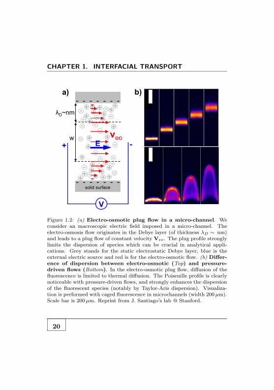
Figure 1.2: (a) Electro-osmotic plug flow in a micro-channel. Weconsider an macroscopic electric field imposed in a micro-channel. Theelectro-osmosis flow originates in the Debye layer (of thickness λD ∼ nm)and leads to a plug flow of constant velocity Veo. The plug profile stronglylimits the dispersion of species which can be crucial in analytical appli-cations. Grey stands for the static electrostatic Debye layer, blue is theexternal electric source and red is for the electro-osmotic flow. (b) Differ-ence of dispersion between electro-osmotic (Top) and pressure-driven flows (Bottom). In the electro-osmotic plug flow, diffusion of thefluorescence is limited to thermal diffusion. The Poiseuille profile is clearlynoticeable with pressure-driven flows, and strongly enhances the dispersionof the fluorescent species (notably by Taylor-Aris dispersion). Visualiza-tion is performed with caged fluorescence in microchannels (width 200µm).Scale bar is 200µm. Reprint from J. Santiago’s lab @ Stanford.
20

1.1. ELECTRO-OSMOSIS
in the nanometer-scale interfacial layer. Moreover, according toEq-1.8 the velocity is robust to downsizing and is insensitiveto the huge increase of hydrodynamic resistance experienced inpressure-driven flow [1].The plug profile of the flow strongly lim-its the Taylor dispersion [2] in the channel which is critical withPoiseuille flow. This makes electro-osmosis a very useful drivingmethod in microfluidics [3]. In particular for chemical analysispurposes which need to displace product without dispersion (seeFig-1.2b.). Conversely electro-osmosis is a common techniquefor pumping fluids [4, 5]. However pumping with DC voltageis limited by slow velocity (typically 100µm/s) and Faradaicreactions at the electrodes. AC applied voltages [6, 7] is there-fore used to increase pumping efficiency as well as more fancyelectrokinetics effects (ACEO, ICEO ..) thanks to non lineareffects [8–10]. The world of electrokinetics is broad and pas-sionating but goes far beyond the basic intuition of interfacialtransport we want to offer.
1.1.4 Electro-phoretic motion of a colloidal par-ticle
Let us consider the effect of an electric field on a colloidal par-ticle with radius R ≫ λD. Zooming at the scale of the Debyelayer, the surface of the colloid appears flat and the consid-ered situation is equivalent to the case of electro-osmosis butwith the fluid at rest. We therefore observe a motion of thecharged colloid in an electric field, namely the electro-phoresis.The derivation of the electro-phoretic velocity VEP requires thecomplete resolution of the Stokes flow around the colloid given
21

CHAPTER 1. INTERFACIAL TRANSPORT
the electro-osmotic slip boundary condition, i.e. V = VEO onthe surface. Assuming that the Debye layer is much smaller thatthe particle radius, it leads exactly to the result for an homoge-neous particle:
VEP =ǫζ
ηE = −VEO
1.9
1.1.5 Electro-osmosis: an interfacial transport
We now point some aspects of the results that are in fact sharedby all phoretic phenomena and deeply related to the interfacialorigin of the mechanism.
• The Debye length is only a few nanometers, and the electro-osmotic velocity Veo appears as an apparent slip velocityon a macroscopic length scale. Dynamical processes in theregion of finite thickness in interaction with a solid surfaceleads formally to a violation of the non-slip boundary con-dition (BC) with consequences on the flow at much higherscale.
• The osmotic velocity does not depend on the geometryof the particle, i.e. the radius of the colloid. Phoretictransport is hence very robust to downsizing and is thusa golden avenue in the advent of micro and nano-fluidics.
• The flow relies on the modifications of a solute –here ions–in the close vicinity of a solid surface through interac-tions –here electrostatic through the zeta potential of thesurface–.
22
1.2. DIFFUSIO-OSMOSIS: MOTION INDUCED BY A
SOLUTE GRADIENT
• The total net force exerted on the colloid is zero which istotally different from situations in which the particle mo-tion is induced by a net body force. In that respect thehydrodynamics flow field differs drastically from the flowfield associated with external fields as gravity. In partic-ular this implies that the 1/r term in the hydrodynamicfield vanishes.
1.2 Diffusio-osmosis: motion induced by
a solute gradient
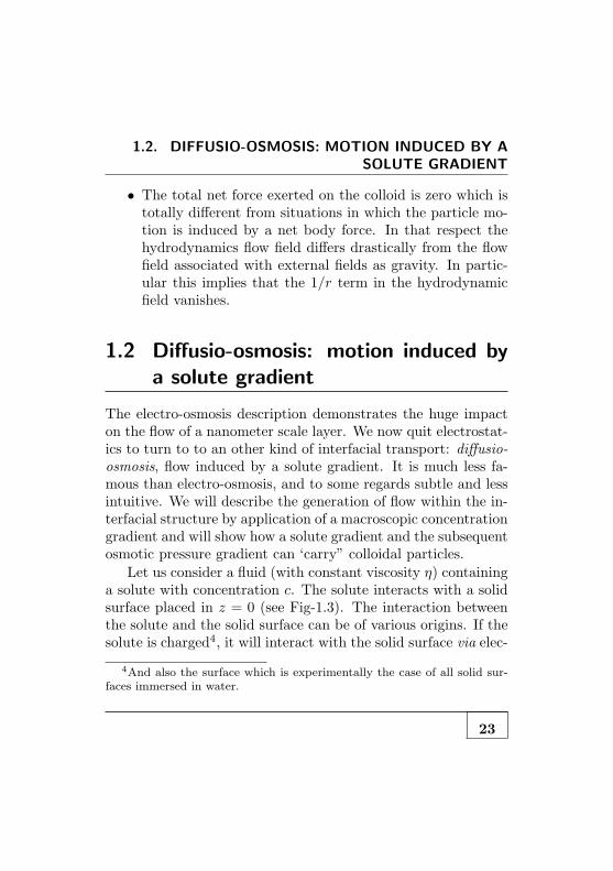
The electro-osmosis description demonstrates the huge impacton the flow of a nanometer scale layer. We now quit electrostat-ics to turn to to an other kind of interfacial transport: diffusio-osmosis, flow induced by a solute gradient. It is much less fa-mous than electro-osmosis, and to some regards subtle and lessintuitive. We will describe the generation of flow within the in-terfacial structure by application of a macroscopic concentrationgradient and will show how a solute gradient and the subsequentosmotic pressure gradient can ‘carry” colloidal particles.
Let us consider a fluid (with constant viscosity η) containinga solute with concentration c. The solute interacts with a solidsurface placed in z = 0 (see Fig-1.3). The interaction betweenthe solute and the solid surface can be of various origins. If thesolute is charged4, it will interact with the solid surface via elec-
4And also the surface which is experimentally the case of all solid sur-faces immersed in water.
23

CHAPTER 1. INTERFACIAL TRANSPORT
trostatic forces leading to a Debye double-layer at the interfacebetween the solid and the liquid phase. It may also result fromVan der Waals interactions between the neutral solutes and thesolid surface.We consider here a potential of interaction U(z) between thesolute and the surface and we define a typical length λ for therange of interaction, e.g. λ is the Debye length λD for electro-statics interactions (see section 1.1.1).At thermal equilibrium, in the dilute limit of non interactingions, it leads to a Boltzmann distribution of the solute species:
c(z) = c0e−
U(z)kBT
1.10
U can be positive (respectively negative) in the case of repulsive(respectively attractive) interactions between the solute and thesurface leading to a depletion (respectively accumulation) of thesolute near the surface5. We point out that the thermal equi-librium may depend on x along the surface (see Fig. 1.3), if theinteraction depends on this coordinate e.g. non uniform zetapotential ζ(x), supposed to vary a length scale a. The resultprescribed in equation Eq-1.10 remains locally valid as long asa ≫ λ.
1.2.1 Solute gradient in the bulk: Fick’s law
We now consider a situation where a concentration gradient ofsolute ∇c0(x) is imposed far away from the surface. In the bulk,
5For electrostatic interactions, a full derivation for the concentration cmust also take into account both anions and the cations of the electrolyteas well as electroneutrality.
24

1.2. DIFFUSIO-OSMOSIS: MOTION INDUCED BY A
SOLUTE GRADIENT
vDO
!
solid surface x
z
Figure 1.3: Diffusio-osmosis of a neutral solute. A solute gradientis additionally imposed along the x direction. The solute interacts withthe solid surface (grey) over the range λ. On the picture, we suppose anattractive interaction between the solute and the surface which leads to anaccumulation of solute at the interface. The solute gradient along the z re-sults in an osmotic pressure (blue arrow, the size of the arrow magnifies theamplitude of the osmotic pressure) which “squeezes” the liquid to the wall.The large scale solute gradient along the x direction gives an unbalancedosmotic pressure in the diffuse layer. That drives the liquid towards theregions of low concentration of solute (supposing attraction between saltand solute). Consequently there is an apparent slip velocity VDO outsideof the interfacial layer which magnitude is given by the balance betweenthe gradient of osmotic pressure in the layer –the motor– and the viscousstress due to the non-slip condition at the solid surface–the dissipation–(see Eq-1.16 and Eq-1.17)
25

CHAPTER 1. INTERFACIAL TRANSPORT
the concentration gradient induces a flux of solute – due to therandom motion of the particles – following the Fick’s law:
JF = −Ds∇c0(x)
with Ds the thermal diffusion of the solute. There is of courseno flux of solvent and thus no flow in a fluid in the bulkinduced by a solute gradient.6
Let us now reconsider this situation from an alternative perspec-tive. The solute concentration gradient may naively be associ-ated to a bulk osmotic pressure given for an ideal solution [11,12]by:
∇Π = −kbT ∇c(x)
1.11
It would thus be tantalizing to think prima facie that the solventflows under the osmotic pressure gradient which is in clear con-tradiction with the previous result. In fact, such an argumentis completely wrong! Indeed, at local equilibrium the mechan-ical –hydrostatic– pressure adapts in order to keep the “total”pressure7 constant everywhere in the bulk according to [13]:
psolvent + kBTc0(x) = p0
1.12
where p0 denotes the pressure in the bulk far from any surface.In bulk the osmotic pressure gradient is counterbalanced by the
6This is exactly true only considering point particles, solvent and solute.Taking into account the size difference between solute and solvent moleculesleads to a solvent flux given the fluid incompressibility. This small effect isnot considered in the following.
7Sum of the solvent and osmotic pressure.
26

1.2. DIFFUSIO-OSMOSIS: MOTION INDUCED BY A
SOLUTE GRADIENT
hydrostatic pressure maintaining the system at rest. In particu-lar, this effect can be used in osmometry. The osmotic pressureΠ exerted by the solute is measured by monitoring the rise ofa solution in vertical tube separated with the pure solvent by asemi-permeable membrane [13].We thus stress that the “bulk” osmotic pressure does not driveany flow in the fluid. We can figure out this effect remember-ing that in the bulk the system does not present any membraneagainst which the force exerted by the solute may act.
1.2.2 Diffusio-osmosis: interfacial transport un-der solute gradient
We now add a solid surface which interacts with the solutethrough an interaction potential U(z). Several orders of magni-tude separate the macroscopic scale of the solute gradient im-posed by an external operator, and the nanometer range λ ofthe interaction. This gives an equilibration time for the concen-tration and the pressure field in the z direction much smallerthan the relaxation for the gradient. Under this assumption,Eq-1.10 rewrites:
c(x, z) ≈ c0(x)e−
U(z)kBT
1.13
The presence of the wall alters the balance between osmoticand hydrostatic pressure. And the mechanical equilibrium ofthe normal forces along z gives:
−∂zp(x, z) +−∂zU(z) c(x, z) = 0
1.14
27

CHAPTER 1. INTERFACIAL TRANSPORT
Using Eq-1.13, Eq-1.14 can be easily integrated and gives the“osmotic equilibrium”:
p(x, z)− kBTc(x, z) = constant = p0 − kBTc0(x)
1.15
where the constant has been determined in the bulk far from thesurface (Eq-1.12). The differentiation of Eq-1.15 with respectto x leads to:
∂xp(x, z) = kBT∂x[c(x, z)− c0(x)]
1.16
A pressure gradient ∇xp rewritten in term of unbalanced os-motic pressure kBT∇x[c(x, z) − c0(x)] acts on the fluid andforces a flow parallel to the surface. As a driving force withinthe diffuse layer it is the motor of the diffusio-osmotic flow. Atmechanical equilibrium this force is balanced by the the viscousshear stress according to Stokes equation.
∂xp(x, z) = η∆vx ∼ η∂2xvx
1.17
where v is the fluid velocity in the layer and the Laplacian op-erator is replaced by ∆ ∼ ∂2
x as the velocity is along x. Finally,the fluid velocity vx(z) increases through the interfacial layer toa finite and constant value VDO in bulk8. Given the non-slipcondition at the wall (Navier boundary condition), double inte-grating the Eq- 1.17, one can determine the velocity profile in
8Once again, we remind that no net force is exerted by a solute gradienton a fluid in bulk.
28

1.2. DIFFUSIO-OSMOSIS: MOTION INDUCED BY A
SOLUTE GRADIENT
the diffuse layer [14, 15]:
V(z) =
∫ z
0
dz′[e−U(z′)/kBT − 1]dc0dx
ex
1.18
and thus obtain the “effective slip velocity” outside the layergiven by Eq-1.18 for z = ∞:
VDO = −(kBT/η)ΓLdc0dx
ex
1.19
where Γ =∫∞
0dz[e−U(z)/kBT − 1] measures the excess of so-
lute induced by the presence of a solid wall (Γ < 0 for de-pletion of solute and Γ > 0 for solid-solute attraction) andL = Γ−1
∫∞
0dzz[e−U(z)/kBT −1] is related to the range of inter-
action of the potential and is thus of the order of λ.
Case of an electrolyte
We consider the particular case of an electrolyte as the soluteand a charged wall characterized by its surface potential ζ in-teracting electrostatically. For the sake of simplicity we supposeanions and cations of the same but opposite charge | q |. Theproblem has been studied previously in section-1.1.1 and we onlyremind that the ions organize in a double layer of typical thick-ness λD screening the surface charge. We can thus conclude thatthe length scale Γ and L are of order λD and Eq-1.19 simplyrewrites:
VDO ∼ −λ2DkBT
η∇c0
1.20
29

CHAPTER 1. INTERFACIAL TRANSPORT
Using the expression for the Debye length, λ2D = ǫkBT/2q
2c0prescribed by the Gouy-Chapman model (see section-1.1.1), oneobtains:
VDO ∼ −DDO∇ log c0
1.21
where DDO = ǫk2BT2/2q2η is the diffusio-phoretic mobility of
the considered electrolyte (and surface). DDO has the dimen-sion of a diffusion coefficient and DDO ∼ 10−10 m2/s –at roomtemperature for a monovalent salt– which corresponds to thethermal diffusion coefficient of a ∼ 2 nm particle in water. Letus stress that DDO only depends on the characteristics of theinterfacial layer as for the electro-osmosis/phoresis phenomena.
Marangoni-like effect in the Debye layerPhysically the diffusio-osmotic velocity VDO can be interpretedfollowing the same reasoning as for electro-osmosis. The drivingforce of the flow is the excess of osmotic pressure ∇(−kBTc0)integrated over the Debye layer, of thickness λD. As λ ∼ nm,it can be expressed as a macroscopic surface stress:
σo ∼ λD ×∇[−kbTc0]
1.22
which is a Marangoni-like stress “−∇γ” with a non uniformsurface tension γ, related to the solute concentration as follows:
γ(x) = λDkBTc0(x)
1.23
The excess of osmotic pressure is balanced by a viscous stresstaking its origin in the velocity gradient in the diffuse layer.Given the non-slip BC at the wall and the diffusio-osmotic ve-locity outside the diffuse layer, the viscous stress can be written
30

1.2. DIFFUSIO-OSMOSIS: MOTION INDUCED BY A
SOLUTE GRADIENT
as:
ση ∼ η
λDVDO
1.24
The mechanical equilibrium σo = ση leads to the “apparent slipvelocity” VDO:
VDO ∼ −λ2DkBT
η∇c0(x)
1.25
as obtained in Eq-1.19. Finally the diffusio-osmotic flow canthus be rephrased as a Marangoni-like effect in the Debyelayer.
Ion specificityThe theory for diffusio-phoresis in electrolyte gradient relies onelectrostatic interaction and does not depend on the type of ionconsidered(at given charge). Actually we have discussed up tonow only the chemio-osmotic mechanism of the diffusio-phoreticflow. In order to take into account the salt ion-specificity mea-sured experimentally [16,17], one has to consider the local elec-troneutrality of the solution. A full treatment for charged speciesmust involve a supplementary electrophoretic contribution origi-nating in the difference of electrophoretic mobilities of the ions.Indeed, an electric field E’ is spontaneously generated in theabsence of electrical current when a concentration gradient ofan electrolyte is established:
je = −(−q)D−∇c0 − qD+∇c0 + (−q)c0µE+E
′ + qc0µE−E
′
1.26
31

CHAPTER 1. INTERFACIAL TRANSPORT
with q > 0 the electrical charge of the cation9, D+ (respectivelyD−) the thermal diffusivity of the cations, (respectively anions)and µE
+, (espectively µE−) the electrical mobility of the cations
(respectively anions). The fluctuation-dissipation theorem re-lates the electrical mobility and diffusivity [13]:
µE± =
±qD±
kBT
We can derive from Eq-1.26 the electric field E’ at zero current:
E′ = βkBT
q∇ log(c0)
1.27
with β = (D+−D−)/(D++D−) quantifies the difference of iondiffusion coefficients and is ion-specific. The self-induced electricfield E’ drives the diffuse layer by electro-osmosis (see section-1.1) at a slip velocity given by the Schmoluchovski formula (Eq-1.8):
V′E = −ǫζ
ηE′ = −β
ǫζkBT
ηq∇ log(c0)
1.28
It contributes simultaneously to chemio-osmosis to the diffusio-osmotic flow. A complete derivation of the problem gives thetotal apparent slip velocity VDO [18]:
VDO = −DDO∇ log(c0)
1.29
with
DDO = −βǫζ
η
kBT
q+
ǫ
2πη(kBT
q)2 log(1− ζ2)
1.30
9For the sake of simplicity we suppose anions and cations with the sameabsolute charge.
32

1.2. DIFFUSIO-OSMOSIS: MOTION INDUCED BY A
SOLUTE GRADIENT
where the first term originates in the self-induced electrophoreticcontribution, and the second term is the complete derivation ofchemio-osmotic contribution. Finally, Eq-1.29 and Eq-1.30 givea complete and quantitative expression of the diffusio-osmoticflow induced by an electrolyte gradient. One can use salt gradients–usually obtained with LiCl, NaCl, KCl– to benchmark the va-lidity of the theory of diffusio interfacial transport. This is donein [17] and in the experiments reported in the chapter 2 of thismanuscript.
1.2.3 Diffusio-osmosis in a nutshell
Focusing on main ingredients and the physics at stake , we fi-nally summarize the diffusio-osmotic mechanism:
1. Role of the imposed solute gradient. A solute gradientalong x gives a gradient along x of the normal osmoticpressure.
2. Role of the surface. The interaction potential U of thesolute with the surface provokes a normal osmotic pres-sure gradient which squeezes10 the fluid against the wall.This normal stress is mediated in the surface plane by theisotropy of the pressure.
Taking into account this two effects, one can thus figure out thata solute gradient along x gives an interfacial pressure gradient
10In the case of an attractive potential
33

CHAPTER 1. INTERFACIAL TRANSPORT
related to the unbalanced osmotic pressure along the same di-rection (see Fig-1.3). It pushes the fluid in the vicinity of thesurface and is at the source of the diffusio-osmotic flow.
1.2.4 Diffusio-phoretic motion of a colloidalparticle
As for electro-phoresis in section-1.1.4, we now consider the ef-fect of a solute gradient on a colloidal particle in the limit ofR ≫ Γ, L with R the radius of the colloid. The diffusio-osmoticflow in the interfacial layer leads to a net motion of the colloid inthe solute gradient, namely diffusio-phoresis. Considering thesame material and the same surface charge for both the colloidand the surface, the diffusio-phoretic velocity reads:
VDP = −VDO = DDO∇ log[c0(x)]
1.31
= DDP∇ log[c0(x)]
1.32
where DDP = DDO defines for consistency the diffusio-phoreticmobility. As for electro-phoresis (see section-1.1.4), the drivingforce acts only in the diffuse layer and gives a “phoretic” ve-locity which depends on interfacial properties but non of theradius of colloid. This gives the phenomenon a high robustnessto downsizing, provided R ≫ L,Γ.Diffusio-phoresis is a ballistic motion along a solute gradient andthus completely different from a diffusive dynamics. We canhowever assess on purely dimensionnal basis that the diffusio-phoretic mobility will compare with natural diffusion in the sys-
34

1.2. DIFFUSIO-OSMOSIS: MOTION INDUCED BY A
SOLUTE GRADIENT
tem and thus with the diffusion constant Dc of the colloid11.The thermal diffusion is given according to the fluctuation-dissipation theorem by the Stokes-Einstein formula: Dc = kBT/6πηR[19–22]. If we consider a colloidal particle of radius R = 0.5µmin water at ambient temperature, Dc ∼ 0.4µm2/s and is thusmuch smaller than DDP ∼ 100 − 500µm2/s. We now considerthe diffusivity of the solute used as a solute gradient e.g. LiClsalt. The thermal diffusion Ds ∼ 1300µm2/s12 is of the sameorder of magnitude as the diffusio-phoretic mobility of the col-loid. This is a hint on the role of carriers exerted by the solutemolecules to drag the big species –the colloid– along the gradientas recently underlined in [17].
1.2.5 General case –New!–
In this section, which may be skipped on a first reading, we comeback on the diffusio-osmosis phenomenon and emphasize the os-motic nature of the process. While most of the chapter is areview of the literature, we point that the following result is anoriginal contribution.We generalize the result of Eq- 1.19 to situations where the os-motic pressure discards the ideal solution which goes as Π =kBTc (see Eq-1.11). This is notably the case for polymer so-
11This intuition will be supported by numerous experimental and theo-retical results in chapter 2.
12For an mulitvalent electrolyte solution for which anion and cation donot present the same diffusivity, the salt diffusivity is defined as detailed
in [23] as Ds =(|z−|+z+)D−D+
z+D++|z−|D−
where D+ and D− the diffusivities of the
consituent ions and z+ and z− their valence.
35
CHAPTER 1. INTERFACIAL TRANSPORT
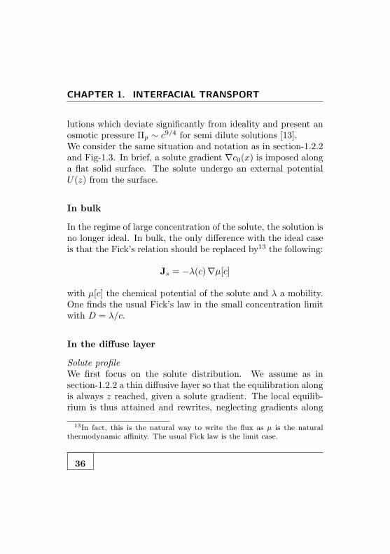
lutions which deviate significantly from ideality and present anosmotic pressure Πp ∼ c9/4 for semi dilute solutions [13].We consider the same situation and notation as in section-1.2.2and Fig-1.3. In brief, a solute gradient ∇c0(x) is imposed alonga flat solid surface. The solute undergo an external potentialU(z) from the surface.
In bulk
In the regime of large concentration of the solute, the solution isno longer ideal. In bulk, the only difference with the ideal caseis that the Fick’s relation should be replaced by13 the following:
Js = −λ(c)∇µ[c]
with µ[c] the chemical potential of the solute and λ a mobility.One finds the usual Fick’s law in the small concentration limitwith D = λ/c.
In the diffuse layer
Solute profileWe first focus on the solute distribution. We assume as insection-1.2.2 a thin diffusive layer so that the equilibration alongis always z reached, given a solute gradient. The local equilib-rium is thus attained and rewrites, neglecting gradients along
13In fact, this is the natural way to write the flux as µ is the naturalthermodynamic affinity. The usual Fick law is the limit case.
36

1.2. DIFFUSIO-OSMOSIS: MOTION INDUCED BY A
SOLUTE GRADIENT
the surface w.r.t. z gradients14 [13]:
µ[c(x, z)] + U(z) = µ[c0(x)]
1.33
Osmotic pressureA general formulation for Π can be expressed with f , the freeenergy density [13]:
Π(c) = c∂f
∂c− f(c) + f(c = 0)
1.34
Pressure profileWe now turn to the pressure profile. It is derived from theprojection of the Stokes equation along z:
0 = η∆vz −∇zp+ c(x, z)(−∂zU)
1.35
with vz = 0 as the flow is along x so that:
∇zp = c(−∂zU)
1.36
Using, Eq-1.33, the right term of Eq-1.36 gives,
c(x, z)(−∂zU) = −c×∇z (µ[c0(x)]− µ[c(x, z)]) = c∇z
(
∂f
∂c
)
T
1.37
14Note that this is the stationary solution of the Smoluchowski equation:∂tc+∇Js = 0, with
Jzs = −λ∇zµ+mc (−∂zU)
with m a mobility. Inserting the equilibrium solution Js = 0, we obtainthe fluctuation-dissipation relationship for the mobilities λ, µ: λ = m× c.
37

CHAPTER 1. INTERFACIAL TRANSPORT
using the thermodynamics definition for the chemical potential
µ =(
∂f∂c
)
T.
Now, using the expression 1.34 for the osmotic pressure, one has
∇zΠ[c] = c×∇z
(
∂f
∂c
)
Altogether,
c(−∂zU) = ∇zΠ[c].
1.38
Coming back to Eq-1.36, one deduces ∇z(p−Π) = 0, and thus
p(x, z)−Π[c(x, z)] = p0 −Π[c0(x)]
1.39
Velocity profileWe now consider the velocity profile projecting the Stokes equa-tion along x:
0 = η∆vx −∇xp+ c(−∂xU)
1.40
The last term being zero, using Eq-1.39, it can be recast intothe expression:
0 = η∆vx −∇x (Π[c0(x)]−Π[c(x, z)])
1.41
The solution of the equation is
vx(x, z) =−1
η
∫ z
0
dz′ z′ ∇x(Π[c0(x)]−Π[c(x, z)])
1.42
38

1.2. DIFFUSIO-OSMOSIS: MOTION INDUCED BY A
SOLUTE GRADIENT
Now using Gibbs-Duhem relation, dΠ = cdµ15, one may rewritethis expression as
vx(x, z) =1
η
∫ z
0
dz′ z′ (c0(x)− c(x, z))∇xµ[c0(x)]
1.43
For this result we also used, accordingly to Eq-1.33, that
∇xµ[c(x, z)] = ∇x (µ[c0(x)]− U(z)) = ∇xµ[c0(x)]
independent of z.Using the Gibbs-Duhem relation
c0(x)∇xµ[c0(x)] = ∇xΠ[c0(x)]
One obtains a more transparent expression for the diffusio-osmoticvelocity:
VDO = KDO ×∇Π[c0(x)]
1.44
with the diffusio-osmotic mobility KDO thus defined as
KDO = −1
η
∫ ∞
0
dz′ z′(
c0(x, z)
c0(x)− 1
)
1.45
This result demonstrates that diffusio-osmotic transport is os-motic by nature and points the osmotic pressure Π as the properthermodynamic variable of interest. It ultimately shows that the“logarithmic-sensing” of the diffusio velocity: VDO ∝ ∇ log c ∼
15Also shown directly: ∇Π = c ∂2c f(c)∇c, while ∇µ = ∂2
c f(c)∇c
39

CHAPTER 1. INTERFACIAL TRANSPORT
∇µ16 (see Eq-1.32) is not related to a gradient of a gradient offree energy as could be thought naively.Additionally the non-linear “sensing”, i.e. the non linear depen-dence of the velocity w.r.t. the solute concentration may orig-inate from non-linearities of the osmotic pressure (as for poly-mers) or from the mobility KDO (case of an electrolyte). Such anon-linearity can be harnessed for interesting out-of-equilibriumproperties as patterning (see section 2.3) which gives the mech-anism a wide range of applicable solute.
16Assuming the case of an ideal solution with chemical potential µ =kBT log(c).
40

1.3. FURTHER INSIGHTS ON DIFFUSIO TRANSPORT
1.3 Further insights on diffusio transport
1.3.1 Massive amplification by hydrodynamicslip
Figure 1.4: Slip length b. The sliplength is the distance in the solid atwhich the linear extrapolation of thevelocity vanishes. Reprint from [1].
We previously reviewed thegeneration of flow, electro-osmotic or diffusio-osmotic,within the diffuse layer byapplication of a macroscopic,respectively electric poten-tial or osmotic pressure gra-dient. As an interfacially-driven phenomenon, we nowreport the impact of slippageon the transport and outlinethe physical ingredients thatlead to its massive amplifica-tion.
Slippage
The question of hydrodynamic boundary conditions for simplefluids has motivated large amount of recent, theoretical and ex-perimental, work recently. Usually, when a simple liquid flowsover a motionless solid wall, its velocity is assumed to be zeronear the wall. This assumption postulated by hydrodynamics iscalled the Navier non-slip boundary condition. Although it iswidely verified for macroscopic flows, the nature of the boundary
41
CHAPTER 1. INTERFACIAL TRANSPORT
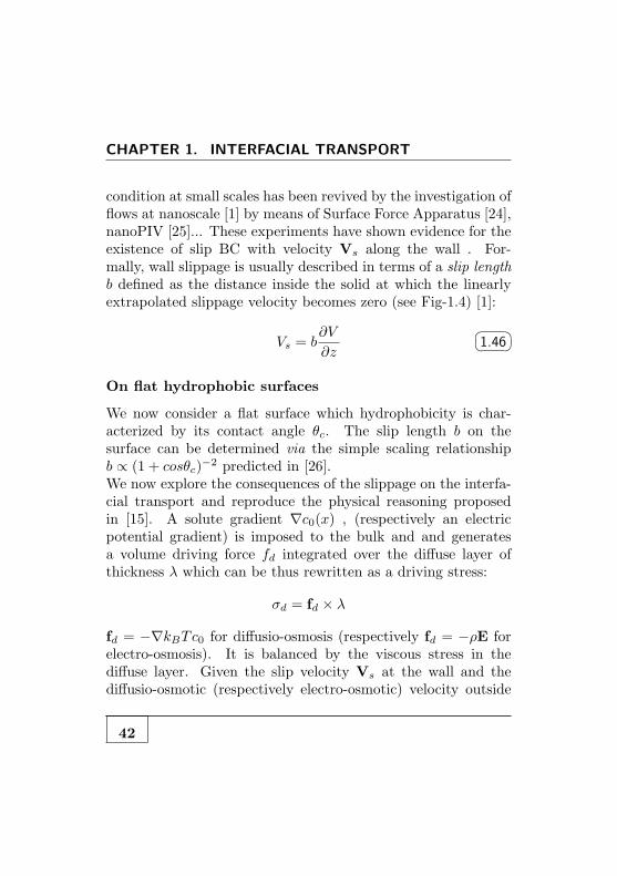
condition at small scales has been revived by the investigation offlows at nanoscale [1] by means of Surface Force Apparatus [24],nanoPIV [25]... These experiments have shown evidence for theexistence of slip BC with velocity Vs along the wall . For-mally, wall slippage is usually described in terms of a slip lengthb defined as the distance inside the solid at which the linearlyextrapolated slippage velocity becomes zero (see Fig-1.4) [1]:
Vs = b∂V
∂z
1.46
On flat hydrophobic surfaces
We now consider a flat surface which hydrophobicity is char-acterized by its contact angle θc. The slip length b on thesurface can be determined via the simple scaling relationshipb ∝ (1 + cosθc)
−2 predicted in [26].We now explore the consequences of the slippage on the interfa-cial transport and reproduce the physical reasoning proposedin [15]. A solute gradient ∇c0(x) , (respectively an electricpotential gradient) is imposed to the bulk and and generatesa volume driving force fd integrated over the diffuse layer ofthickness λ which can be thus rewritten as a driving stress:
σd = fd × λ
fd = −∇kBTc0 for diffusio-osmosis (respectively fd = −ρE forelectro-osmosis). It is balanced by the viscous stress in thediffuse layer. Given the slip velocity Vs at the wall and thediffusio-osmotic (respectively electro-osmotic) velocity outside
42
1.3. FURTHER INSIGHTS ON DIFFUSIO TRANSPORT
the diffuse layer, the viscous stress reads:
ση ∼ ηVO
λ+ b
1.47
using the definition of the slip length b as the equivalent position,in the solid, where the non-slip BC would apply. The mechanicalequilibrium finally gives an effective slip velocity V b
O, enhancedby the hydrodynamic slip, by a factor 1 + b/λ where λ measurethe interfacial thickness:
VbO ∼ −(1 + b/λ)
λ2
ηfd ∼ (1 + b/λ)V0
O
1.48
where V0O stands for the effective slip velocity without slippage
and VbO with a slip length b.
The enhancement of interfacial transport, notably electro or dif-fusio osmosis, by hydrodynamic slippage can actually be verylarge. For molecular solutes, the interaction range can be veryshort: λ ∼ 0.3 nm. As the slip length can be up to b ∼ 20−30 nm[24] on smooth hydrophobic surfaces, one can expect giant am-plification of the flow by a factor of 100, or at least by an orderof magnitude !
On superhydrophobic surfaces
Previous results encourage to increase the slip-length to magnifyeven more the amplification of the transport. In this scope therecent development of artificial superhydrophobic (SH) surfaces,which couple chemical hydrophobicity with multi and large scaleroughness with exceptional non wetting properties (θc ∼ 180)
43

CHAPTER 1. INTERFACIAL TRANSPORT
seem to be a relevant avenue to take up the challenge. Indeed, itwas shown that one could define an “effective slip length” beffon SH surface up to a few microns. With beff/λ ∼ 102−104 onthese surfaces, one could expect massive amplification of interfa-cial transport, and thus extremely efficient microfluidic pumpingbased on electro-osmosis or chemical diffusio-osmotic transduc-tion. In fact the problem is slightly more tricky and the massiveamplifification depends on the interfacial transport: no amplifi-cation is obtained for electro-osmosis on SH surface while am-plification of more than 3 orders of magnitude can be achievedfor diffusio-osmosis. This result was recently obtained in [27] bymolecular dynamics (MD) simulations and we will only give abasic idea of the physical reasons which make diffusio-osmosisand electro-osmosis so different on SH surfaces.
We consider a SH surface with slipping length beff (see Fig-).As for smooth surface, the effective slip velocity V beff is givenby:
Vbeff
O∼ −(1 + beff/λ)
λ
η〈Fd〉eff
1.49
where 〈Fd〉eff is the “effective” driving force integrated over thediffuse layer, i.e. averaged over the pattern.
Electro-osmosisAs liquid-air interface is not charged, the driving force of theelectro-osmotic flow only takes place in the regions where theliquid is in contact with the solid surface. One thus expressesthe effective driving force on SH surface 〈Fd〉eff in terms of the
44

1.3. FURTHER INSIGHTS ON DIFFUSIO TRANSPORT
integrated driving force F0d on a smooth, non slipping surface :
〈Fd〉eff ∼ ΦsFd
1.50
with Φs ∼ a/L the solid fraction of the SH surface where a andL are characteristics of the SH surface. a is the typical lengthscale for solid/liquid contact areas and L is the roughness peri-odicity and height.Using the expression of the effective slip length beff ∼ a/Φs asin [28] and gathering Eq-1.49 and Eq-1.50, one does not expecta large increase of the velocity [29]. This scaling argument hasbeen confirmed numerically by MD simulations [27]. Super hy-drophobicity does not amplify electro-osmotic transport as thedriving force is reduced as much as the viscous dissipation onsuch surfaces.
Diffusio-osmosisWe now turn to the case of diffusio-osmosis which is signifi-cantly different. The key point is that due to the interactions ofions with the air-water interface (e.g image charge repulsion ofspecific adsorption), a diffuse layer still exists at the air water-interface (contrary to electro-osmosis) [30]. The driving forceFd is thus approximately uniformly distributed and the effec-tive driving force on SH surface rewrites:
〈Fd〉eff ∼ Fd
1.51
Finally using Eq-1.49, one gets a giant amplification of thediffusio-osmotic flow by a factor beff/λ ∼ 1000 on SH surfaces.
45

CHAPTER 1. INTERFACIAL TRANSPORT
These theoretical expectations still remain to be supported andused experimentally to reach a new class of “high velocity” mi-crofluidic flows.
1.3.2 Thermo-phoresis vs Diffusio-phoresis
We discussed previously the motion of a colloidal particle undera solute gradient or an electric field. We now present a very briefoverview of an other class of interfacial transport, the motion ofa particle induced by a temperature gradient, so called thermo-phoresis.
Thermo-phoresis
When a colloid is placed in a temperature gradient ∇T0(x), itpresents a steady drift velocity along the gradient [31]:
VT = −DT∇T0(x)
1.52
where DT is the thermo-phoretic mobility, positive for thermo-phobic particles and thermophilic otherwise. Most colloids pref-erentially move to colder regions while macromolecular soluteas DNA present thermophilic characteristics.For most investigated systems, the order of magnitude of | DT |is rather universal and varies within a limited range 10−12 <|DT |< 10−11 m2/s−1K−1. But predictions on the mobility aretedious and strongly depend on the system [31]. Additionallythe sign of DT may depend on the temperature and presenta temperature inversion T ∗ of thermophobic to thermophilictransition. Moreover a size dependance of the mobility recently
46

1.3. FURTHER INSIGHTS ON DIFFUSIO TRANSPORT
reported [32] and unexpected for interfacial transport recentlyreported is at the core of a controversy feeding experimentaldebate as well as theoretical developments [32–34].
Thermo-phoresis vs Diffusio-phoresis in microfluidics
Gradient establishmentWe consider a microfluidic situation with a channel filled withparticles. An external operator imposes a gradient of solute(respectively temperature) to move particles by diffusio-phoresis(respectively thermo-phoresis) across the channel. The gradientis imposed through boundary conditions, i.e. side of the channeldistant of a length ℓ, and the typical time to achieve the steadygradient is dimensionally given by τ ∼ ℓ2/K where K is thediffusivity of the considered observable, i.e. K = Ds the solutediffusion coefficient for diffusio-osmosis andK = λT the thermaldiffusivity. The thermal diffusivity of water is λT ∼ 106 µm2/sand thus much larger that the diffusivity of a typical soluteDs ∼ 1000µm2/s which gives for the transient time:
τT ∼ τDP /1000 ≪ τDP
For ℓ ∼ 100µm which is a typical scale for microfluidic channels,τT ∼ 10−2 s while it can take up to 10 s to develop the solutegradient.
Response timeThe time τ can be seen on a slightly different perspective asthe “response time” of the system. Let us imagine now that
47

CHAPTER 1. INTERFACIAL TRANSPORT
the external operator varies the boundary conditions with a fre-quency f . If τ ≫ 1/f , the gradient does not develop and thus nophoretic motion of particles is observed. For smaller frequencies1/f ≫ τ , the phoretic migration is recovered. The microfluidicsystem behaves as a low-pass filter of cutoff frequency f∗ = τ−1
for the interfacial transport of particles.In this scope, the thermo-phoresis appears as a high speed mi-crofluidic tool as it can respond to high frequency 10− 1000Hzstimuli while diffusio-phoresis is strongly limited in its microflu-idic applicability by very low response time (10−100 s). Thanksto the use of IR laser which makes possible to heat locally,the developments of the thermo-phoresis in microfluidics [35,36](or more generally temperature driven motion [37,38]) are nowbooming.The counterpart of the high-speed response is a fast relaxationfor thermo-phoresis. If for some reasons the BC fluctuate thethermal gradient is modified by these fluctuations and the relax-ation of the gradient once the external constraints are releasedis very fast. In order to take advantage of controlled thermo-phoresis, a system must provide a steady energy supply whichis very costly. This might be the reason why thermo-phoresisin nature is up to now only reported in geological systems suchas hydrothermal pores [39]. On the contrary, the slow parti-cle diffusion transport smoothens changes in BC and make thegradient quite robust to fluctuating environments. Moreover atrack of the gradient lasts for seconds even after suppressing theBC. In that respect, one could imagine that living micro-systemsmay use diffusio-phoresis as a relevant transport phenomenon ofmacromolecules inside the cell in the noisy biological environ-
48

1.4. TAKE HOME MESSAGE
ment. Nevertheless, this point is for now purely speculativeas no diffusio-phoretic flow has ever been reported in micro-organisms.
1.4 Take home message
Surface-driven transport thus appears as particularly interest-ing in the scope of micron-size systems. The flow generationin the diffuse layer at the solid-liquid interface by field gradient(electric potential, temperature, concentration) appears as an“effective slip velocity” at the wall and thus strongly impactsthe velocity profile on much higher scale.In this manuscript, I will mainly focus on diffusio-phoretic trans-port: motion induced by a solute gradient. This phenomenonhas been little studied experimentally and thus needs furtherexperimental and theoretical investigations. Furthermore, itproposes in essence a transducer of free energy into mechani-cal power. This opens new routes in a context of new sources ofenergy by harnessing natural solute gradient. Moreover, a giantamplification of the effect is expected with SH surfaces whichmakes of diffusio an outstanding avenue for high efficiency mi-crofluidic pumps and chemical-mechanical transducers.Two natural scenarii can be considered for diffusio-phoresis: (i)an external operator imposes a solute gradient and particlesmove within or (ii) particles generates autonomously the gradi-ent and propel. I have developed these two axes during my PhDon two different classes of systems: microfluidics and swimmers.
49

CHAPTER 1. INTERFACIAL TRANSPORT
1. Microfluidic. I have designed a specific hydrogel microflu-idic technology and device to maintain and accuratelycontrol spatially and temporally solute gradients. Sucha setup makes it possible to study the diffusio-phoreticmigration of particles in a controlled environment.
2. Swimmers. I have synthetized self propelled micro-swimmersusing a catalytic reaction on one half of a colloid to gener-ate the solute gradient. These active particles constitutethe building bricks for the study of collective behaviorsof suspensions of self propelled particles thus intrinsicallyout-of-equilibrium.
Each of the scenario is a chapter of this thesis manuscript.
50
C’est veritablement utile puisque c’est joli
A. St Exupery, Le Petit Prince
2Diffusio-phoresis in a controlled
gradient : a gel device
In the previous chapter we have focused on simple physical ar-guments to build an intuition of interfacial and particularlydiffusio-phoretic transport. We now turn to an experimentalinvestigation of the phenomenon. Pioneering works were per-formed with membranes to establish the solute gradient, thusintroducing additional complexity both into the experience andinto the data analysis [16] or poor control of the gradient inmacroscale experiments [40,41]. Recently the use of microfluidictool has made possible to study the diffusiophoretic migrationof colloids in a well-defined electrolyte gradient [17,42]. Quanti-tative agreement with theoretical diffusio-phoretic behavior hasbeen recently achieved by Abecassis et al. and the experimenthas shown (i) a solute driven motion of colloids and (ii) a steadyobservations under flow. This microfluidic setup also leads to
51

CHAPTER 2. DIFFUSIO-PHORESIS IN A CONTROLLED
GRADIENT : A GEL DEVICE
quantitative predictions of the solute gradient but no temporalor spatial control.
Aim of this work
An important achievement of my PhD has been to develop anduse new experimental approaches allowing to go one step beyondin the exploration of diffusio-phoresis phenomena. This requires(i) the building-up of controlled concentration gradients and (ii)the observations of particles in a convection-free environment.We have therefore developed a specific microfluidic device basedon an agarose hydrogel technology, studied diffusio-phoretic mi-gration and unveiled new osmotically-driven effects.
Organization of the chapter
This chapter first begins with a presentation of the experimen-tal setup. In particular we demonstrate how to generate aconvection-free spatial gradient, together with its temporal ac-tuation.In a second part, we use this experimental device to study thediffusio-phoretic migration of various particles, colloids as wellas biological macromolecules, in a benchmark configuration andcompare our results with the theoretical expectations. Then thehydrogel microfluidic device is used to unravel new osmotically-driven effects such as patterning and localization. The local-ization process with time-dependent solute gradients originatesin the non-linearity of the diffusio-phoretic velocity and is ratio-nalized by an asymptotic model of rectification of oscillations as
52

well as numerical predictions. Conversely another trapping orlocalization is also demonstrated in a transient “osmotic shock”provided by the extreme sensibility of the logarithmic sensing ofdiffusio-phoresis to vanishing solute concentrations.We finally discuss a few perspectives of study of diffusio-phoresisboth fundamentaly or applied to microfluidic applications. Wewill end up by putting forward an iconoclast questioning on thepossible role of diffusio-phoresis in living soft matter as concen-tration gradients are common in living organisms.
Principle
The detailed study of diffusio-phoretic motion relies on our abil-ity to generate and control concentration gradients. Followingthe route proposed for the study of bacterial chemotaxis in amicrofluidic environment [43, 44], I have developed a microflu-idic device made of agarose hydrogel. The principle of the finaldevice is sketched in Fig. 2.1. It relies on the porous nature ofthe hydrogel [45]: the hydrogel matrix acts as solid walls for theflow but allows the free diffusion of salt and small molecules.In a nutshell, a solute gradient is created across the systemby imposing two different concentrations in boundary channels:the source, with concentration c1 = c0, and the sink c2 = 0.An external operator can therefore control the gradient in amicrofluidic chamber at rest, i.e. without any flow containingthe particles (colloids or DNA) under investigation. The set-up, sketched in Fig. 2.2-a, allows to impose stationary, as wellas temporally switchable, solute gradients in various microflu-
53

CHAPTER 2. DIFFUSIO-PHORESIS IN A CONTROLLED
GRADIENT : A GEL DEVICE
C C 1
C C 2
ColloidsHydrogel Colloids Colloids C1 C2
Hydrogel
Glass cover slip
Side view
Figure 2.1: Principle of the hydrogel microfluidic device. The porousnature of the gel makes possible to impose solute boundary conditions withconcentration c1 and c2 via two side channels and thus control the con-centration gradient. Particles under investigation are enclosed in a centralchamber.
idic designs1. Although the present manuscript will essentiallyfocus on the experimental study -using this new device- of differ-ent physical phenomenon, it should be stressed that the develop-ment of the setup itself is actually an important achievement ofthis PhD work, and mobilized a large amount of work to ensurea proper reliability and reproducibility. Overall, experimentaland technical details corresponding to the final configuration aregathered in Appendices A to C for the sake of clarity and a morepleasant reading.
Globally, a solute gradient, here either of fluorescein, or of asalt2 or a molecular species as H2O2 is created in the central
1The microfluidic design is made of two side channels along microfluidicchambers of various sizes (typically 300-600µm) and shape (rectangular orcircular).
2We have used LiCl, NaCl and KCl salts.
54

2.1. CALIBRATION OF THE GRADIENT
microfluidic chambers containing the particles via two side chan-nels imposing the concentration boundary conditions. The lat-ter can be switched on demand thanks to a manual microfluidicswitch that allows modification of the side-channels solute con-centrations. After a transient due to the diffusion of boundaryconditions across the middle item of the device, a steady profileof the gradient is reached. The concentration gradient is thesolution of the diffusion equation:
Ds∆c = ∂tc
2.1
with Ds the salt diffusivity and the boundary conditions givenby the concentration c1 and c2 injected by the syringe pump inthe two side channels.Under stationary conditions, the equation 2.1 reduces to ∆c = 0which gives at one dimension a linear profile for the concentra-tion with slope (c2 − c1)/ℓ, with ℓ the distance between sidechannels. For a 2D circular geometry, the solution is given byseries of Bessel functions according to the boundary conditions.
2.1 Calibration of the gradient
The gradient profile is calibrated using a fluorescein solution(Roth) of concentration c0 = 10−4 M. In this range of con-centration, Diao et al. showed a linear relation between thefluorescein concentration and fluorescence intensity [43] mak-ing a fluorescent measurement a straightforward visualizationof the chemical concentration field in the channel. A syringe
55

CHAPTER 2. DIFFUSIO-PHORESIS IN A CONTROLLED
GRADIENT : A GEL DEVICE
x/w!
Flu
o. In
ten
sit
y (
A.U
)
outlet
Agarose
channels Fluorescent colloids
Objective
Glass slide
a) C2
C1 T/T0
2
0 1 T/T0
Switch
b) Linear Steady Gradient
0 1
x
C2
C1
w
0
ℓ
1
Microfluidic chamber
w
Temporally Tunable
x/w
c)
T/T0
!C
/w (
A.U
)
0.5 -0.5
S.S S.S
Tr Tr
Figure 2.2: (a) Experimental Setup. hydrogel microfluidic device. Adouble syringe pump with two solutions of salt of concentration c1 and c2fills the two side channels. A microfluidic switch allows to exchange the saltsolutions in the side channels, leading to a time-dependent tuning of thegradient. Particles under investigation (colloids and λ-DNA) are located inthe center microfluidic chamber.(b)-(Left) Visualization of the fluorescein gradient. Top view of themicrofluidic device setup. The inner box shows the experimental fluores-cence intensity image measured for the stationary gradient (gel walls notrepresented) of a fluorescein solution (c1 − c2 = 10−4M)). The centralchamber width is w = 300µm while ℓ = 800µm is the total diffusion width(scale bar is 300µm). (b)-(Right) Steady fluorescence intensity pro-files. Steady linear concentration gradient. Temporal changes in boundaryconditions upon actuation of the microfluidic switch lead to gradient inver-sion (red and blue curves). (c) Temporal evolution of the gradient –for periodic actuation T0 = 10mins– of the difference ∆c of fluorescence in-tensity on both sides of the central chamber following a gradient inversion.Orange arrows stand for steady gradients whereas the black ones stand fortransient states.
56

2.1. CALIBRATION OF THE GRADIENT
pump fills one channel with a fluorescein solution of concentra-tion 10−4 M (the source) and the other with distilled water (thesink). A manual switch allows to invert the role of source andsink and thus reverse the gradient. Measurements are performedfor linear channels i.e. linear side channels and a rectangularmicrofluidic chamber. In the following experiments we did notobserve interactions between the electrolyte solutions we usedand the hydrogel structure of the microfluidic device.
Steady concentration gradientWe consider a linear 1D geometry and define x = 0 in the middleof the microfluidic chamber. The length scale ℓ is the length overwhich the gradient develops, i.e. the distance between the sidechannels as defined previously. The boundary conditions aregiven by c(−ℓ/2) = c1 and c(ℓ/2) = c2. As previously stated, asteady profile of the solute concentration is achieved, with slope(c2 − c1)/ℓ. The concentration can be written as:
c(x) =c02(1± 2
x
ℓ)
2.2
± depending whether the source is the side channel on ±ℓ/2.The concentration profile is measured via the fluorescence inten-sity of fluorescein (see Fig. 2.2-b). As expected for this geometry,the steady gradient is linear. The microfluidic switch allows toreverse the role of source and sinks and therefore to mirror thegradient with respect to the center of the channel (red and bluecurves). I checked experimentally that the solute flux in thesource/sink was sufficient to define constant boundary condi-tions along the channel. This can be understood in terms of a
57

CHAPTER 2. DIFFUSIO-PHORESIS IN A CONTROLLED
GRADIENT : A GEL DEVICE
definition of a Peclet number. The Peclet Pe ≡ τD/τC comparesthe diffusive time τD for the boundary conditions to diffuse alongthe length scale ℓ to the convective time τC for the fluid to gofrom the inlet to the outlet. In our experiments, τD = ℓ2/Df ,
τC = L/U and therefore Pe = ℓ2UDfL
where L ∼ 10 cm is the
length of the side channels, U ∼ 3 cm/s the velocity of the in-jected solutions, ℓ ∼ 800µm and Df = 420µm2/s [46], thefluorescein diffusion coefficient. Under the present conditions,the Peclet number is of order Pe ∼ 450, much larger than unity.This ensures the stability of the boundary conditions both dur-ing the calibration step and the experiment as LiCl diffusesfaster than fluorescein salt3.
Transient concentration gradient.Following the reversal of the side boundary conditions, the con-centration profile is in a transient state. As a diffusive process,the transient duration τtr thus scales as ℓ2/D. Experimentalvisualization of the transient gradient is performed once againwith a fluorescein solution monitoring the temporal evolution ofthe difference ∆c of the fluorescence intensity on both sides ofthe central chamber (see Fig-2.2-c). Both steady and transientstates are represented on this figure. After a sharp increase dur-ing the transient state, ∆c is constant. We nevertheless observea slow increase of the difference of the concentration. We at-tribute this “drift” in fluorescence intensity to the 3D diffusion
3Indeed the diffusion constant for LiCl is D′s = 1360µm2/s which cor-
responds to a Peclet number of Pe′ ∼ 140.
58
2.2. DIFFUSIO-PHORETIC MIGRATION
of the fluorescent salt at the top of the microfluidic chamber4.We measure a transient time τtr ∼ 2mins for fluorescein andℓ = 800µm. One can then estimate the transient time for LiClsalt given the diffusion constant of fluorescein Df = 430µm2/sand LiCl salt Ds = 1360µm2/s [47]. It gives a typical transienttime τtr ∼ 430
1360 × 2min ∼ 35 s.Finally after after a few tens of seconds for salts, wecan assume a linear and steady concentration profile inthe microfluidic chamber containing the particles under investi-gation.
2.2 Diffusio-phoretic migration
We now consider the situation where particles have been en-closed in the central chamber. We first concentrate on the caseof latex colloids of diameter 200nm. The step by step protocolto perform an experient, i.e. (1). mold the hydrogel micro-fuidics and (2). fill a microfluidic chamber with the particlesunder investigation is thoroughly developed in Appendix B andC at the end of the chapter.
59

CHAPTER 2. DIFFUSIO-PHORESIS IN A CONTROLLED
GRADIENT : A GEL DEVICE
t=0s
t=90s
t=180s
t=270s
20
0!
m
0
1
Figure 2.3: Diffusio-phoretic migration of fluorescent colloids to-wards high concentration of LiCl. The salt concentration normalized by c0is sketched by the lateral bar.
2.2.1 Diffusio-phoretic migration in a solutegradient: first approach
We start from a configuration where all particles are on oneside of the channel. At t = 0 the salt gradient is reversed withnow the high concentration on the opposite side. Under theimposed solute gradients, the colloids are observed to exhibita purely transverse motion (see Fig-2.3). The drift is alongthe salt concentration gradient and towards the higher soluteconcentration thus revealing a diffusio-phoretic migration
4Indeed the channels are typically 100µm high while the PDMS spacerdefines agarose stamps of thickness 700µm. As a consequence, a 600µmlayer of gel is at the top the channels/chambers
60

2.2. DIFFUSIO-PHORETIC MIGRATION
of the colloids thanks to a salt gradient (see Fig-2.3). Thediffusio-phoretic velocity is of order 1µm/s. When particleshave gathered at the opposite wall, the gradient is reversed againthus showing a symmetrical behavior with a reversed transversemotion (see Fig. 2.4-a and supplementary movie 1).
2.2.2 Experimental validation
Before a quantitative analysis of the diffusio-phoretic transportof particles in a controlled gradient, we want to underline a fewexperimental validation of the designed microfluidic device.
Experimental checks
I first checked that without any salt gradient the colloids dy-namics is purely Brownian. A slight longitudinal drift can beobserved in some experiments by the following of a few bunchesof colloids as markers. The upper bound for this occasional driftspeed is 50 nm/s which is small compared to the diffusio-phoreticvelocity of the particles and thus negligible. We infer this aDarcy flow through the porous gel5. This observation may ap-
5The pressure gradient originates in the pressure drop due to thePoiseuille flow in the side channels. The pressure gradient induced bythe flow in lateral channel is of order ∇P ∼ − η
h2 U with η the viscosityof the solution, h ∼ 100µm the height of the microfluidic chamber and Uthe velocity of the injected solution. This pressure gradient is transmittedthrough the gel walls to the microfluidic chamber and induces flow alongthe chamber thanks to the porosity of the gel. At steady state, the drift inthe chamber is related to the pressure gradient by the Darcy relationshipVdr = −κ
η∇P (b). For a flow velocity U ∼ 5 cm/s and a Darcy permeabil-
61

CHAPTER 2. DIFFUSIO-PHORESIS IN A CONTROLLED
GRADIENT : A GEL DEVICE
pear trivial but actually constitutes an essential test. First, thereproducible and reliable absence of leakage is not an easy taskto reach in microfluidics. Second, devicing an observation cham-ber maintened at rest with residual drifts of only a few nm/sgoes far beyond the standard accuracy required in microfluidics,even for pressure-driven flows.
Sedimentation
We use 200 nm latex colloids with a sedimentation length δ =kBT/mg ∼ 100µm, with kB the Boltzmann constant, T theroom temperature, m the boyant mass of colloid and g the grav-ity6. δ is thus of the same order of magnitude as the height of themicrofluidic chamber (h ∼ 120µm) which provides a reasonablevertical uniformity of the colloid concentration. Additionally,the sedimentation velocity7 vsed = mg/6πηR for these particlesis typically vsed ∼ 1 nm/s which ensures a weak effect of the sed-imentation during the typical time of an experiment (∼ 1−2 h).Finally, combined with the solute gradient calibration by flu-orescence, these control experiments and order of magnitudecalculations demonstrate that our microfluidic device can gen-erate a tunable and steady gradient in a chamber con-taining particles with no convective flow and withoutany leakage.
ity κ ∼ 500nm2 (extracted from the litterature for a 3% agarose gel [48]),we obtain Vdr ∼ 2.5 nm/s which is in reasonable agreement with what weobserved experimentally.
6This result will be discussed thoroughly in chapter 3.7η being the viscosity of the fluid and R the radius of the colloid.
62

2.2. DIFFUSIO-PHORETIC MIGRATION
2.2.3 Analysis of the experiments
Quantitative analysis
In order to quantify the diffusio-phoretic motion, we plot infigure 2.4-b the time dependent location of the colloid popula-tion. It is defined as the maximum of the fluorescence intensityprofile, measured using image analysis (Matlab)8. As can beseen, the observed drift is close to linear with a slight devia-tion observed at long times. Neglecting the transient regime(lasting about 30-60s for salt, see section 2.1), the stationarysalt concentration takes the form: c(x) = c0
2 (1 ± 2xℓ ), with ℓ−1
the slope of the concentration gradient, and x the distance tothe center of the observation channel. Using the expression ofthe diffusio-phoretic velocity VDP = DDP
∇cc (see Eq-1.32) in a
steady linear concentration (see Eq-2.2), the position X0 of acolloid obeys the equation:
dX0
dt= ±DDP
1(
ℓ
2±X0
) ,
2.3
± depending whether the source is the side channel on ±ℓ/2.Initially, all colloids are concentrated at a position X0(t = 0) =∓w/2 where w denotes the width of the central channel. For
8The process is the following. First, the intensity profile is averagedon the all picture to give a 1D profile. Then the maximum of the profileis determined. In order to limit the influence of intensity fluctuations inthe profile, a local quadratic fit of the intensity is carried to determine theposition of the maximum of intensity, X0.
63

CHAPTER 2. DIFFUSIO-PHORESIS IN A CONTROLLED
GRADIENT : A GEL DEVICE
a)
b)
c)
d)
time (s) time (s)
positio
n (!
m)
time time Colloids DNA
Figure 2.4: Diffusiophoretic transport of fluorescent colloids andλ-DNA under a LiCl gradient. (∆cs[LiCl] = |c2 − c1| = 100mM witha 1mM buffer in both channels to fix the pH (TRIS buffer for colloids andTRIS-EDTA buffer for DNA). Central channels are 200µm (a) or 300µm(c) wide with an identical ℓ = 800µm, scale bar 100µm). (a)-(c)). Motionof particles under a salt gradient, sketched by the lateral bar, towardshigher salt concentrations. Images are separated by 90 s for the colloidsand for DNA the images were taken at t =100, 150, 200, 300 s. (b)-(d)Time evolution of the particles population location characterizedby the maximum in particles density (measured from fluorescence inten-sity). Experimental data (symbols) are fitted according to the theoreticaldescription Eq-2.3 (dashed lines), with DDP as the only fitting parameter(see text). In (b), open symbols correspond to a subsequent migration, andfully superimposes on the previous results. The solid straight line in (b) isa guide line corresponding to constant drift velocity. Shaded regions corre-spond to time periods where wall effects prevent from proper fluorescencemeasurements.
64

2.2. DIFFUSIO-PHORETIC MIGRATION
short times dX0/dt = ±2DDP /(ℓ∓w) and the maximum of thecolloid density exhibits a quasi-linear dependence on time, asobserved experimentally in figure 2.4-b. For longer time, slightdeviations from the linear dependence are expected from equa-tion 2.3 and indeed observed in figure 2.4-b. Physically, thesenon-linearities in X0(t) take their origin in the logarithmic-sensing obeyed by the diffusio-phoretic phenomenon, i.e. thefact that the velocity is proportional to the gradient of the log-arithm of the concentration (see Eq-1.32). The diffusiophoreticvelocity VDP is thus expected to decrease during the migrationin a linear solute profile. Furthermore, given the experimentalinitial conditions X0(t = 0) = ∓w/2, equation 2.3 can be ana-lytically solved and leads to:
DDP t =
X20/2 + ℓX0/2− w2/8 + wℓ/4 if c(ℓ/2) = c0
X20/2− ℓX0/2− w2/8 + wℓ/4 if c(−ℓ/2) = c0
2.4
Overall, Eq-2.4 provides an excellent fitting expression for theexperimental data (Fig. 2.4-b) and gives access to the colloidsdiffusio-phoretic mobility DDP (see Table 2.5). We used thismethod to measureDDP for various salts and obtain the diffusio-phoretic mobility of latex colloids with great accuracy for LiCl.For NaCl and KCl salt, the migration is slower and the dif-fusive spreading of the colloid population increases. The de-termination of the maximum X0 becomes less accurate whichaffects the diffusio-phoretic mobility DDP determination. Al-ternatively, diffusio-phoretic mobilities can be determined withthe total crossing time Tcr, rather than the full dynamics of the
65

CHAPTER 2. DIFFUSIO-PHORESIS IN A CONTROLLED
GRADIENT : A GEL DEVICE
population maximum. Indeed, equation 2.4 for t = Tcr rewritesDDPTcr = f(w, ℓ), where f depends only on geometrical param-eters: w and ℓ, fixed on a serial of experiments. Given a couple(Tcr, DDP ) for a salt, the diffusio-phoretic mobility D′
DP of anunknown salt can thus be determined measuring the crossingtime T ′
cr following:
T ′cr/Tcr = D′
DP /DDP
This “integrated” method yields to DDP similar to the valuesdetermined by fitting without describing the complete displace-ment X0(t). In the case of colloids, the diffusiophoretic mobilitywas measured for three different salts, exhibiting values for themobility in the order LiCl>NaCl>KCl (see Table 2.5). Thissalt specifity effect is predicted by the theory. As a quick re-minder, it takes its origin in the difference of diffusivity betweenanions and cations of a salt and consequent self-induced-electro-phoresis (electro-phoretic contribution of diffusio-phoresis, seesection 1.2.2-ion specificity in the previous chapter).
While most of the experiments have been conducted with col-loids in salt gradients, the physical mechanism explored is notlimited to this “colloids in electrolytes” configuration. We thenturn to the diffusio-phoretic migration of alternative systemssuch as “biological colloids” (DNA) in salt gradient or colloidsin a neutral solute: hydrogen peroxyde.
66

2.2. DIFFUSIO-PHORETIC MIGRATION
Figure 2.5: Value for the diffusiophoretic mobility DDP extractedfrom the channel crossing experiments (see text). Experimental trapstrength K extracted from the trapping experiments (see section 2.3) andcompared to the predicted value from Eq-2.8.
Diffusio-phoretic migration of biological macromolecules
First, the moving particles are not bound to be spherical colloidsbut can also be macromolecules. As a demonstration, the samemotility experiments as presented above in figure 2.4-a,b werealso conducted with λ-DNA: phage-λ DNA (48kbp, Fermentas,Germany) diluted 10 times in Tris-EDTA buffer is enclosed inthe microfluidic chamber (see Appendix B and C of this chap-ter for more experimental details). A salt gradient -LiCl, NaCl,KCl- is imposed via the boundary conditions in the hydrogel mi-crofluidic chamber. The solute gradients induces the migrationof the biological colloid (gyration radius of typically 200 nm) to-wards the high concentration of salt (see Fig. 2.4-c,d). We thendemonstrate the motion of DNA molecules under salt concentra-tion gradients. The determination of the diffusio-phoretic mobil-ity of DNA by the fitting method is more tedious as the non lin-earity of the velocity is much higher for the experiment than for
67

CHAPTER 2. DIFFUSIO-PHORESIS IN A CONTROLLED
GRADIENT : A GEL DEVICE
simple diffusio-phoresis predictions (see Table 2.5). This resultshows that the simple prediction (Eq 1.32) derived for sphericalsolid colloids does not fully capture the specifity of the dynamicsof a complex macromolecule as DNA. For example, the gyrationradius of DNA can depend on the salt concentration throughthe screening of charges as well as the zeta potential of thispolymeric ball. Nevertheless we confirme the diffusiophoreticmigration of DNA towards higher concentrations of salt.
Diffusio-phoretic migration in a neutral solute
As a final remark, we emphasize that salt is used here because ofits simplicity, other solutes could be used as an alternative. The-oretically, a diffusio-phoretic migration will occur with any so-lute having non-vanishing interactions with the particle [15,23],while the details of such interaction (attractivity, repulsivity,strength, etc.) determines the amplitude and direction of theparticle response. Experimentally, the diffusio-phoretic responsewith neutral polymer as solutes have indeed been recently ob-served [36]. We here further demonstrate experimentally thediffusio-phoretic migration with a non-charged specie: the hy-drogen peroxide H2O2 solution. In contrast to LiCl, NaCl orKCl salt gradients, latex colloids escape the high concentrationof hydrogen peroxide. H202 acts as a repellent for latex colloids(DDP < 0)9.
9This sign for DDP must originate at microscopic scale in a depletionof H2O2 molecules at the solid latex surface according to Eq-1.19.
68

2.2. DIFFUSIO-PHORETIC MIGRATION
To summarize, we have shown that the diffusio-phoreticmigration of particles in electrolyte thus exhibits threemain features: motility driven by concentration gra-dient, salt specificity effects and logarithmic-sensing.Moreover, the logarithmic expression of the velocity VDP =DDP∇ log c presents two specificities: (i) it is non linear and(ii) the velocity “diverges”10 when the solute concentration goesto zero. In the following, we will address each of this point andshow how it leads to versatile and interesting localization pro-cesses.
10In the limit of our model
69

CHAPTER 2. DIFFUSIO-PHORESIS IN A CONTROLLED
GRADIENT : A GEL DEVICE
2.3 Trapping by rectified diffusio-phoresis
As noted previously, the diffusio-phoretic motion in electrolytegradients is characterized by a logarithmic-sensing which intro-duces a slight non-linearity in the velocity to concentration re-lationship. Such a non-linearity actually suggests that underperiodic oscillations of the salt gradients, a rectification of theparticles motion may be induced: we now explore this featurefor particles trapping and patterning.
2.3.1 Osmotic trapping of colloids
While the diffusiophoretic migration was studied under a sta-tionary gradient, we now generate concentration gradients os-cillations as in figure 2.2-b,c by periodic inversions of the con-centration boundary conditions (period T0). As stated in theprevious section, we choose T0 ∼ 6− 10mins depending on thesalt and therefore on the crossing time. We start from an ho-mogeneous concentrated population of colloids (F8888, 200 nm,Molecular Probes) in the central chamber11. After each oscilla-tion the population of colloids is depleted close to the wall of thechannels and after 3-4 oscillations, the colloids are trapped inthe center of the channel. The period of oscillations is then re-duced and the band keeps oscillating around the center with the
11As previously detailed the concentration profile of the colloids insidethe chamber is imaged by the spatial fluorescence intensity in the chamberwith a 20x objective. The fluorescence intensity is strongly attenuated bymicroscope filters and shutted between pictures to limit colloids bleachingphenomenon.
70

2.3. TRAPPING BY RECTIFIED DIFFUSIO-PHORESIS
salt cycles, but its width remains stationary. The experiment isshown in Fig. 2.6-a) for colloids: starting from a homogeneousdistribution, the particles population evolves after a few cyclestowards a band with a stationary width. This band is Gaussianto a very good approximation (see Fig. 2.6-a). Note that theprocess is robust: starting from inhomogeneous particles distri-bution, or changing the oscillation frequency -within our limitedaccessible range as specified earlier- yields the same width forthe trapped band. Finally as for the colloids motility, the widthof the trapped band depends on the salt nature: LiCl > NaCl> KCl in terms of trapping efficiency.Additionally, we also performed similar experiments with λ-DNA as motile particles: Fig. 2.6-b) shows that trapping isequally achieved with macromolecules, namely biological col-loids, the latter gathering also in a narrow band with Gaussianprofile. Despite a slow migration of DNA and a low DDP whichshould in principle limit the trapping efficiency, the experimen-tal observations show very effective localization. This originatesin the strong non-linearity of the DNA diffusio-phoretic migra-tion (see figure Fig. 2.4-b): the front particles nearly stop whilethe back ones still advance. This makes the trapping easy andefficient.
2.3.2 Principle in a nutshell
We now present a cartoon picture that captures the physics atwork in the phenomenon of particles segregation observed dur-ing experiments with oscillating concentration gradients. Con-sider that one syringe pump contains a salt with given concen-
71

CHAPTER 2. DIFFUSIO-PHORESIS IN A CONTROLLED
GRADIENT : A GEL DEVICEIn
tensity (
A.U
)
Colloids DNA a)
x/ℓ x/ℓ
-0.1! 0.1! -0.1! 0.1!
b)
Figure 2.6: Trapping under salt gradient oscillations. Trapping ofcolloids, (a), and λ-DNA with YOYO-1, (b), under salt gradient oscillations(buffers and salt concentration as in Fig. 2.4; T0 = 600 s). (Top): Startingfrom a homogeneous population, the particles focus to a band of stationarywidth (scale bar 100µm), independent of the oscillation frequency (300 µmwidth channels with 250 µm gel walls). (Bottom): symbols, experimentalparticles density profile in stationary state, as obtained from the fluores-cence images; dashed line, Gaussian fit from which experimental trappingstrengths K are deduced through K = kBT/σ2, with σ the Gaussian width.They are compared to theoretical expectations according to Eq-(2.8) in Ta-ble 2.5.
72

2.3. TRAPPING BY RECTIFIED DIFFUSIO-PHORESIS
tration c0 while the other syringe contains only buffer. For thesake of simplicity, we will first suppose that the linear steadyprofile of the gradient is instantaneous reached after a reversalof the boundary conditions i.e. we neglige the transient regime.Initially, we suppose that the high concentration of the salt is onthe right side of the chamber: source on the right, sink on the left(see Fig. 2.7) . A colloid on the left side on the chamber at t = 0will migrate to the right thanks to diffusio-phoresis phenomenon(see Fig. 2.7-a). After a time T0/2, the colloid has crossed a partof the chamber and the salt gradient is reversed. The colloid at-tracted by the high concentrations of salt reverse the directionof its motion and migrates to the left (see Fig. 2.7-b). At timeT0, the concentration gradient is reversed and so on... After oneperiod and a complete oscillation of the boundary conditions,the colloid has experienced a net displacement to the center ofthe chamber (see Fig. 2.7-c). After a few oscillations, any colloidinitially in the chamber ends up in x = 0. In other words, undera constant solute gradient, the velocity of particles is larger inregions with smaller solute concentration. Accordingly, the frontparticles move slower than the ones at the back: iterated overthe oscillations, such a process leads to the observed focusing.This phenomenon takes its origin in the logarithmic-sensing ofthe diffusio-phoretic migration in electrolyte solutions (see Eq-1.32). The distance covered during the first half-period [0;T0/2]is not the same during the second half-period [T0/2;T0]. Afterone period the colloid motion is therefore rectified towards thecenter of the channel.Through this cartoon, we have pictured the phenomenonof trapping by rectified oscillations of concentrations.
73

CHAPTER 2. DIFFUSIO-PHORESIS IN A CONTROLLED
GRADIENT : A GEL DEVICE
From cartoon to real life: time scales in the real experiment.In the cartoon picture of the trapping phenomenon we neglect–for the sake of simplicity– the transient state of the gradient.Nevertheless as we pinpointed in section 2.1, after a switch ofthe syringe, the side channels must be refilled by the new so-lution and boudary conditions need finite time to diffuse fromthe side channels to the microfluidic chamber. Therefore, a realexperiment is slightly more complex that the previous sketch.Experimentally, the trapping scenario must take into account3 different time scales: the transient time Ttr to refill the sidechannels and for the salt to diffuse through ℓ, the time Tcr for acolloid to cross the chamber and finally the oscillation period T0
of the concentration gradient. In order to follow the trappingscenario, T0 is smaller than Tcr. In addition, to limit limit-sizeeffects and accumulation of colloids blocked along the chamberwalls, T0 must be taken much lower than the crossing time. Butit must also be bigger than the transient time Ttr to assume rec-tified linear concentration gradient with good approximationAnideal trapping experiment thus follows Ttr ≪ T0 ≪ Tcr.With constant ℓ = 800µm in all experiments, the transienttime is Ttr ∼ 30 − 60 s (see section 2.2) and the crossing timeTcr ∼ 7 − 15mins. Given the experimental parameters – givenchannel geometry and colloids– the oscillation period is the onlyexperimentally tunable parameter. It is chosen in the range 6to 10mins i.e. the time for colloids to cross typically 1/5 to 1/3of the channel.
74

2.3. TRAPPING BY RECTIFIED DIFFUSIO-PHORESIS
a) b)
c)
Figure 2.7: Sketch of the phenomenon of trapping by rectified os-cillations of concentrations. We suppose instantaneous reversals of thesteady linear concentration profile (solid black line). The boundary condi-tions oscillate with a period T0. Only the microfluidic chamber containingthe colloids (red circles) is represented with the gel walls (blue). Color ar-rows stand for the colloids displacements.For clarity, effects are accentuated.The velocities are represented accordingly to equation 1.32: V ∼ ∇c/c. (a)0 < t < T0/2, the source channel on the right, the sink is on the left.The colloids migrate towards the high concentration of salt, i.e. on theright. The colloid on the left is faster than on the right given the expres-sion for the diffusio-phoretic velocity. At T0/2, the boundary conditionsare reversed and the reversed linear profile is instantaneously reached. (b)T0/2 < t < T0, the migration is reversed to the right towards the regionsrich of salt. Once again, the colloid in the lower concentration region isfaster. (c) After one oscillation, the colloids has experience a net displace-ment to the center. This trapping effect is thus a direct consequence of thenon linear dependance of the velocity with the concentration.
75

CHAPTER 2. DIFFUSIO-PHORESIS IN A CONTROLLED
GRADIENT : A GEL DEVICE
2.3.3 Theoretical Predictions
In order to get further insight into the trapping mechanism atwork, we have conducted a detailed investigation of the parti-cles dynamics. As we now show, the trapping of the particlesresults from the rectification of their motion under the oscillat-ing driving field of the salt concentration. The rectification isaccordingly induced by the non-linear sensing of the diffusio-phoretic motion, VDP ∝ ∇[log c] (see Eq-(1.32)) where c(x, t)stands for the salt concentration field.
Our starting point for the modelization is the Smoluchowskiequation for the particles concentration, ρ(x, t), here coupled tothe salt diffusive dynamics:
∂tρ = −∇ · (−Dc∇ρ+DDP∇[log c]ρ)
∂tc = Ds∆c
2.5
with Dc the particle diffusion constant, Ds that of the salt withconcentration c and DDP the particle diffusio-phoretic mobility.These equations are coupled to the time-dependent boundaryconditions for the salt concentration: every T0/2, the salt con-centration at the boundaries switches from 0 to c0 for one sideand vice-versa for the other side. At time t = 0 the particlesrepartition is chosen homogeneous12. The geometry fits that ofthe experiments, with particles confined in the central channelwhile the salt gradient develops over the central channel and thegel walls.
12But various initial conditions of the particles population could be im-plemented.
76

2.3. TRAPPING BY RECTIFIED DIFFUSIO-PHORESIS
Numerical Resolution
In a first step, the above coupled equations 2.5 are solved numer-ically using Matlab R©. The geometry as well as the boundaryconditions match the experiments. The salt concentrations inthe side channels oscillate with a stepwise function of periodT0. Accordingly the gel walls are implemented in the numeri-cal simulations as impermeable frontiers only for particles anda free-diffusion medium for salt.The problem is made dimensionless, using ℓ as the unit of lengthand determining the unit of time with Ds. Additional variablesare the following: x ≡ x/ℓ, t ≡ t/τ with τ ≡ ℓ2/Ds. Andthe diffusion coefficient expresses in units of the salt diffusiv-ity: Ds = 1, Dc ≡ Dc/Ds and DDP ≡ DDP /Ds. For anmulitvalent electrolyte solution for which anion and cation donot present the same diffusivity, the salt diffusivity is defined
as Ds = (|z−|+z+)D−D+
z+D++|z−|D−
where D+ and D− the diffusivities of
the consituent ions and z+ and z− their valence [23]. In thefollowing, Dc is set to 0.0016 to match the experimental valuefor colloids of diameter Φ = 200 nm in a LiCl salt. Finally, thecoupled partial equations are solved with Matlab in 1D withDc/DDP as the variable parameter.Results are shown in figure 2.8-a. Starting from a homogeneousspatial distribution of colloids in the channel, after a short tran-sient of a few oscillations the particles population focuses withina band with a stationary and constant width. In these simula-tions the oscillation period T0 = 470 s is chosen as in the ex-periments. We checked that except for the first oscillation thewall effects are limited and that the trapped state is not a con-
77

CHAPTER 2. DIFFUSIO-PHORESIS IN A CONTROLLED
GRADIENT : A GEL DEVICE
sequence of the accumulation of the colloids against the wall.The colloids population is additionally very well described by aGaussian distribution (see Fig. 2.8-b) while its center positionoscillates with the solute oscillations, as observed experimen-tally. We also checked that the trapped state does not dependon the initial conditions: a homogeneous as well as a dirac-like distribution relax to the same steady Gaussian distribution.Moreover we tested the independence of the trap with the oscil-lation period T0 varying the period in the same range as in theexperiments Numerical simulations allow to test conditions thatare not accessible in our experiments as very thin gel walls whichexperimentally do not prevent from leakage. Indeed we couldsuppress gel walls in our simulations13 to increase the range ofaccessible T0. Once again, modifying the oscillation frequencydoes not affect the final state.Consequently the final Gaussian state depends neitheron the oscillation period nor on the initial distributionof colloids nor on the presence of confining walls.Finally we explored numerically the influence on the trappedstate of the ratio DC/DDP in the range 10−2 to typically unity.For DC/DDP < 10−2, ie high diffusio-phoretic mobility, the col-loid migration is fast and the assumption of time scale separationbetween transient gradient and crossing-time breaks. Thereforecolloid population goes from one side to the other and “crashes”the gel walls systematically. The distribution is never steadyand artificially narrowed by periodic blockage against the wall.
13The removal of the walls does not affect the transient time Ttr as thelength scale ℓ is not modified and the salt freely diffuses in walls.
78

2.3. TRAPPING BY RECTIFIED DIFFUSIO-PHORESIS
For low diffusio-phoretic mobility DC/DDP > 1, the colloid mi-grates so slowly that the thermal diffusion spreads the distribu-tion in the whole channel. The population is weakly trapped andas a large number of colloids is close to the walls, side effects cannot be neglicted anymore. In the range 10−2 < DC/DDP < 1,the numerical results suggest a width of the Gaussian distribu-tion σ scaling as σ ∝ ℓ
√
Dc/DDP, with a prefactor 1/2 (seeFig. 2.8-c).
Asymptotic model
A simple asymptotic interpretation of the above results can beproposed. First, due to the fast salt diffusion, one may neglectthe gradient establishment thanks to the diffusion of the bound-ary conditions. The solute concentration profile thus writes as:
c(x, t) = c0/2 + c0f(t)x/ℓ
2.6
with x distance to the channel center, ℓ ≡ c/∇c the distanceover which the gradient establishes and f(t) a time-dependentfunction, oscillating with the salt concentration oscillation pe-riodicity T0. Typically in our experiments, f(t) is a ±1 step-function, in the limit of immediate renewal of the side channelssolutions, so that 〈f(t)〉 = 0 while 〈f(t)2〉 = 1 6= 0, with 〈·〉 thetime average over T0.Now, as in the first part of the study, the mean position X0(t)of the particle population is expected to obey Eq-2.3. For smallexcursions around the center (X0 ≪ ℓ), one can write
dX0/dt ≃ 2DDPf(t) [1− 2f(t)(X0/ℓ) + . . .] /ℓ
2.7
79

CHAPTER 2. DIFFUSIO-PHORESIS IN A CONTROLLED
GRADIENT : A GEL DEVICE
!"
#"
T/T
0
a)
Dc/DDP x/!
Collo
id d
ensity
-0.1 0.1
$%&'" %" %&'"
!"!#
!"!!
!"!$
!"!#
!"!!
!2/l
2
'"
x/!c)
b)
Figure 2.8: Numerical resolution of the particles dynamics underoscillating salt gradients: (a) Spatio-temporal evolution of the col-loid density ρ, where parameters have been set according to experimentsFig. 2.6-a): for Ds = 1360µm2/s, Dc/Ds = 0.0016, Dc/DDP = 0.01,ℓ = 800µm, w = 300µm and T0 = 470 s. White borders represent thegel walls. The color code ranges from blue (low density) to red (high den-sity). (b) Instantaneous particles distribution: (blue circles) initialdistribution, t = 0; (red circles) stationary state distribution; (dashedline) Gaussian profile fit. (c) Evolution of the normalized squaredGaussian width (σ/ℓ)2 as extracted from figure 2.8-b) as a function ofDc/DDP : (red cercles) numerical simulations; (dotted line) fit with linearrelationship, according to theoretical prediction (Eq-2.8).
80

2.3. TRAPPING BY RECTIFIED DIFFUSIO-PHORESIS
In this limit of fast salt oscillations14, one expects the distri-bution in steady state to behave to leading order as ρ(x, t) ≃ρ(x −X0(t)), i.e. the distribution is steady in the reference ofthe mean position of the population. Inserting this guess intothe Schmoluchowski equations for the particles gives:
J = −Dc∇xρ+ V ρ
≃ −Dc∇xρ+2DDPf(t)
ℓ [1− 2f(t)(X0/ℓ)]× ρ
Making the variable change yields δx = x − X0(t) and aver-aging out the fast salt variables yields to 〈J〉 = −Dc∇δxρ +(4DDP/ℓ
2)〈f2〉δx × ρ. Altogether, at steady state 〈J〉 = 0, wepredict a stationary Gaussian distribution for the particles:
ρ(δx) ∝ e−δx2
2σ2 with σ =1
2
√
Dc
DDPℓ
2.8
The gaussian distribution is steady in the reference of the meanposition X0 and oscillates as a whole around the channel centralposition.The asymptotic model stresses the origin of the trap-ping. The non linearity of the diffusio-phoretic velocitygathers the particles ultimately up to a Dirac distribu-tion, while the natural thermal diffusivity of the colloidswidens the trap. Finally the steady state is of Gaussianshape with a width which results from the balance be-tween the diffusio-phoretic narrowing and the Brownian
14corresponding to fast gradient oscillations compared to the time evolu-tion of the colloids distribution T ′
1 ∼ ℓ2/(4DDP)
81

CHAPTER 2. DIFFUSIO-PHORESIS IN A CONTROLLED
GRADIENT : A GEL DEVICE
motion spreading.The predicted Gaussian shape and the expression of its widthare in full agreement with the above numerical resolution of thecoupled dynamics (see Fig. 2.8-b,c). Indeed the the numericalresults collapse on the master curve derived from this asym-potic model with small discrepancies only observed in regimesfor which the wall effects are not negligible (DC/DDP > 1) orfor which the time scale separation assumption clearly breaks(DC/DDP < 10−2).We also point that this trapping process can be formally inter-preted in terms of an harmonic “osmotic” trapping potential,
Vtrap(x) =1
2
kBT
σ2x2.
2.9
While the kBT prefactor suggests an entropic origin, the trap-ping process is non-equilibrium in its root. Furthermore, thetrapping strength is accordingly characterized by an harmonicstrength K = kBT/σ
2. The experimental values for the mea-sured trapping strength K are gathered in Table 2.5 for vari-ous salts. These are compared to the theoretical predictions,in which DDP was set to the mobility measured independentlyin channel-crossing experiments (Fig. 2.4). Results in Table 2.5show a good agreement between experimental trapping and pre-dicted theoretical values from Eq-(2.8). A final important re-mark is that the trapping potential is strong: over the cell-chamber scale –with overall size ℓ– the trapping free-energy wellhas a depth of ∆F ≈ kBT
DDP
Dc∼ 100kBT .
82

2.3. TRAPPING BY RECTIFIED DIFFUSIO-PHORESIS
2.3.4 Pattern symmetry versus temporal sig-nal
We now generalize the previous results to more complex geome-tries in order to demonstrate the robustness and generic char-acter of the above scenario. To this end, we have tested thissegregation phenomenon in a circular, “cell shaped”, chamber.
Experimental observations
The experimental setup is derived from the previous experi-ments replacing a rectangular by a circular chamber and modify-ing the side channels in order to impose a gradient of circular ge-ometry. A sketch of the channels is represented in figure 2.9-a,b:a circular chamber (650µm in diameter) is surrounded by twoside-channels conveying the salt and the particles –here colloidswith 200 nm of diameter – are initially homogeneously spreadin the chamber. Two different concentration gradient forcingsare explored: an antisymmetric forcing where the salt bound-ary concentrations c1 and c2 are switched periodically between0 and c0 with antisymmetric phase as in the previous section;and a symmetric forcing where c1 = c2 switches periodically be-tween 0 and c0 in phase . We want to stress here that the originof the diffusio-phoretic migration depends on the nature of theforcing. The colloids move thanks to the steady concentrationgradient in the antisymmetric driving, but the transient gradi-ent -between two steady states of constant salt concentration-is the source of the migration in the symmetric case.As demonstrated in figures 2.9-c,d, the salt oscillations again
83
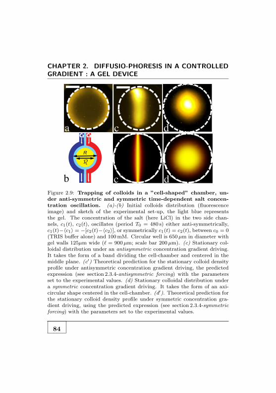
CHAPTER 2. DIFFUSIO-PHORESIS IN A CONTROLLED
GRADIENT : A GEL DEVICE
a! c! d!
b! d’!c’!
R
R
Figure 2.9: Trapping of colloids in a ”cell-shaped” chamber, un-der anti-symmetric and symmetric time-dependent salt concen-tration oscillation. (a)-(b) Initial colloids distribution (fluorescenceimage) and sketch of the experimental set-up, the light blue representsthe gel. The concentration of the salt (here LiCl) in the two side chan-nels, c1(t), c2(t), oscillates (period T0 = 480 s) either anti-symmetrically,c1(t)−〈c1〉 = −[c2(t)−〈c2〉], or symmetrically c1(t) = c2(t), between c0 = 0(TRIS buffer alone) and 100mM. Circular well is 650µm in diameter withgel walls 125µm wide (ℓ = 900µm; scale bar 200µm). (c) Stationary col-loidal distribution under an antisymmetric concentration gradient driving.It takes the form of a band dividing the cell-chamber and centered in themiddle plane. (c′) Theoretical prediction for the stationary colloid densityprofile under antisymmetric concentration gradient driving, the predictedexpression (see section 2.3.4-antisymmetric forcing) with the parametersset to the experimental values. (d) Stationary colloidal distribution undera symmetric concentration gradient driving. It takes the form of an axi-circular shape centered in the cell-chamber. (d′). Theoretical prediction forthe stationary colloid density profile under symmetric concentration gra-dient driving, using the predicted expression (see section 2.3.4-symmetricforcing) with the parameters set to the experimental values.
84

2.3. TRAPPING BY RECTIFIED DIFFUSIO-PHORESIS
produce a localization of the particles in the cell chamber (seealso supplementary movies 3 and 4). Furthermore the symmetryof the pattern depends directly on the symmetry of the driving:one observes a linear localization with a“cat eye” shape for theantisymmetric driving, and a circular egg-shape localization forthe symmetric driving. This demonstrates the versatility of thetrapping process. Once again, we observed experimentally thatthis localization process is also robust versus the initial distri-bution of the particles.
Theoretical predictions
These different experimental patterns can be understood alongsimilar lines as above. A prediction for the trapping potentialassociated with the particles localization is obtained by averag-ing out the fast salt variables.We consider the circular cell-like configuration sketched in Fig. 2.9.The colloids are embedded in an inner chamber with diameterR, while the salt boundary condition ring has a diameter R (seeFig. 2.9-b). The salt concentration c(r, θ, t) obeys the diffusionequation
∂tc = Ds∆c
with boundary conditions depending on the nature of the forc-ing.
Antisymmetric forcingFor the antisymmetric geometry with T0-periodic temporal in-version of the boundary conditions, the boundary conditions
85

CHAPTER 2. DIFFUSIO-PHORESIS IN A CONTROLLED
GRADIENT : A GEL DEVICE
rewrites with the polar coordinates r, θ:
For 0 < t < T0/2, c(R/2, θ, t) =
c0 if θ ∈ [0;π]0 if θ ∈ [π; 2π]
For T0/2 < t < T0, c(R/2, θ, t) =
0 if θ ∈ [0;π]c0 if θ ∈ [π; 2π]
As for the 1D linear geometry, we neglect the gradient establish-ment due to the diffusion of the boundary conditions and con-sider only the steady concentration profile given by ∆c(r, θ, t) =0. The solution of this equation given the boundary conditionstakes the form:
c(r, θ, t) =c02
[
1 +δ(r, θ)
R/2f(t)
]
2.10
with δ(r, θ) = 4π
∑
k,odd1k (r)
ksin[kθ], and f(t) the periodic step-
like function with period T0. Averaging over the flux of particlesover the fast salt oscillations the stationary colloid density pro-file is then obtained as
ρ[r, θ] ∝ exp
[
−1
2
DDP
Dc
δ(r, θ)2
(R/2)2
]
2.11
Symmetric forcingFor the symmetric geometry, a uniform ring of salt oscillatesperiodically between 0 and c0 and the boundary conditions takethe form:
86

2.3. TRAPPING BY RECTIFIED DIFFUSIO-PHORESIS
c(R/2, θ, t) = cb(θ, t) =
c0 for 0 < t < T0/20 for T0/2 < t < T0
which rewrites with Fourier series:
cb(θ, t) =c02
1 +4
π
∑
k,odd
1
ksin[kωt]
=c02
1 +4
π
∑
k,odd
1
kIm[exp(jkωt)]
with ω = 2π/T0.Here the steady concentration is uniform and one has to takeinto account the transient concentration profile. One obtainsthe salt concentration in the form
c(r, t) =c02[1 + δ(r, t)]
with δ(r, t) = 4π
∑
k,odd1k Im (fk(r) exp[j kω t]).
For each mode kω, fk is the 2D solution of the steady diffu-sion equation and rewrites with the Bessel function of order 0
I0(r/δk), with δk =√
jDs
k ω , the salt diffusive length. By super-
position, the salt concentration rewrites:
cb(r, t) =c02
1 +4
π
∑
k,odd
1
kIm
[
exp(jkωt)I0(
rδk)
I0(R2δk
)
]
87
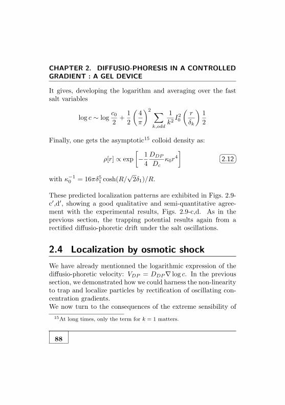
CHAPTER 2. DIFFUSIO-PHORESIS IN A CONTROLLED
GRADIENT : A GEL DEVICE
It gives, developing the logarithm and averaging over the fastsalt variables
log c ∼ logc02
+1
2
(
4
π
)2∑
k,odd
1
k2I20
(
r
δk
)
1
2
Finally, one gets the asymptotic15 colloid density as:
ρ[r] ∝ exp
[
−1
4
DDP
Dcκ0r
4
]
2.12
with κ−10 = 16πδ51 cosh(R/
√2δ1)/R.
These predicted localization patterns are exhibited in Figs. 2.9-c′,d′, showing a good qualitative and semi-quantitative agree-ment with the experimental results, Figs. 2.9-c,d. As in theprevious section, the trapping potential results again from arectified diffusio-phoretic drift under the salt oscillations.
2.4 Localization by osmotic shock
We have already mentionned the logarithmic expression of thediffusio-phoretic velocity: VDP = DDP∇ log c. In the previoussection, we demonstrated how we could harness the non-linearityto trap and localize particles by rectification of oscillating con-centration gradients.We now turn to the consequences of the extreme sensibility of
15At long times, only the term for k = 1 matters.
88

2.4. LOCALIZATION BY OSMOTIC SHOCK
diffusio-phoresis to vanishing electrolytes concentration. No-tably, it is expected from the expression of the diffusio-phoreticvelocity that a vanishing gradient can lead to measurable veloc-ity provided that the solute concentration is low enough. Weexplore further this point via experiments in an “osmotic shock”configuration.
2.4.1 Experimental observations
We start with a solution of 200 nm latex colloids in solutionwith LiCl salt of concentration c0 = 100mM. The colloidalsuspension is enclosed in a microfluidic chamber soaked withLiCl salt solution (see Fig. 2.10-a).At t = 0, distilled water plus buffer is injected with the syringe-pump and the boundary conditions (BC) for the salt are thuschanged from c = c0 to c = 016. The salt concentration in thechamber relaxes by diffusion and reaches in the long time limitthe conditions imposed by the BC: c = 0. During this process,the colloids are observed to strongly concentrate in the centerof the cell (see Fig. 2.10-b) and the migration surprinsingly lasts15− 16mins. For longer time, the Brownian motion dominates,the colloids do not focus anymore and the distribution widensby thermal diffusion of the colloids.
16In the following, we will omit the buffer and thus write that the saltconcentration is c = 0. The important role of the buffer will be explicitlydiscussed further in the section.
89

CHAPTER 2. DIFFUSIO-PHORESIS IN A CONTROLLED
GRADIENT : A GEL DEVICE
a b
Figure 2.10: Localization by osmotic shock. Circular well is 650µmin diameter with gel walls 125µm wide (ℓ = 900µm; scale bar 200µm).Initially, the colloid solution and the gel are in a LiCl salt solution of con-centration c0 = 100mM of salt. For t < 0, salt concentration is thushomogeneous, with value c0 in the system. (a) Initial colloids distribution(fluorescence image). A t=0, boundary conditions c = 0 is imposed by asyringe pump. And for t > 0, the concentration profile relaxes to reach inthe long time limit c = 0. (b) The system undergoes an “osmotic shock”and the colloids move towards the high concentration of salt, e.g. the centerof the chamber. The migration lasts up to 15mins leading to an efficient fo-cusing of the colloid population. The colloid distribution thereafter spreadsby Brownian diffusion.
90

2.4. LOCALIZATION BY OSMOTIC SHOCK
2.4.2 Principle in a nutshell
The directed motion to the center of the cell is of course ofdiffusio-phoretic origin as the salt concentration is higher in thecenter of the chamber than close to the wall (see Fig. 2.11) wherethe salt is sucked by side channels acting as sinks. At steadystate, the salt concentration is zero and homogeneous. As pre-viously discussed in benchmarks experiments, the steady stateshould be reached after ∼ 1min which makes the experimen-tal observations surprising. Actually, a key point of diffusio-phoresis with electrolytes originates in the expression of the diffusio-phoretic velocity V ∝ ∇c/c. This makes the diffusio-phoreticdrift very sensitive to regions where the concentration vanishes(c → 0), as long as ∇c
c 6= 0. We anticipate that this log-sensingof the velocity is at the origin of the long term evolution –over15mins– of the colloid migration. We now present a formalderivation of the colloidal density ρ(r, t) under an osmotic shock.It will develop and underline the role of the logarithmic expres-sion of the velocity in such a long term evolution.
2.4.3 Theoretical predictions
The aim of this part is to obtain the equation for the colloidaldensity, ρ(r, t). To this end we first need to describe the evolu-tion of the solute concentration which drives the colloidal mo-tion. The description is derived in a 2D circular cell and theparameters are set to the experimental values.
91

CHAPTER 2. DIFFUSIO-PHORESIS IN A CONTROLLED
GRADIENT : A GEL DEVICE
0 10.50
0.2
0.4
0.6
0.8
1
t
x/!
C/C
0
Figure 2.11: Solute concentration evolution during an osmoticshock. Initially, c = c0 uniform (blue line). At t > 0, BC c(x = 0, t) = 0and c(x = ℓ, t) = 0 are imposed with side channels as sink. The solute con-centration evolves and relaxes with time to c = 0. Numerical resolutionsof the 1D diffusion equation for t =0, 20 s, 50 s, 100 s, 150 s and 200 s forLiCl salt. Orange arrows stand for the diffusio-phoretic migration of la-tex colloids towards high concentration of salt. Osmotic shock localizationoriginates in the high sensibility to this solute gradient.
92

2.4. LOCALIZATION BY OSMOTIC SHOCK
Solute dynamics in an osmotic shock configuration
The salt concentration c obeys the diffusion equation, togetherwith the boundary conditions at the chamber perimeter. For theosmotic shock the boundary conditions are c(r = R, t < 0) = c0and c(r = R, t > 0) = 0 (same notations as for the trapping ina circular chamber).We first determine a basis of separable functions c = f(t).g(r)solutions of the time-dependent diffusion equation. We get
f ′/f = Ds∆g/g = −K
K being a constant. Developing the Laplacian operator in cylin-drical geometry to agree with the experimental geometry, g issolution of the following ODE: r2.g′′+r.g′+r2. KDs
g = 0. After a
change of variables u = r.√
K/Ds, we obtain a Bessel equationof order 0 defined at r = 0 [49]. Therefore, g(u) = J0(u) whereJ0 is the Bessel function of first kind. Boundary conditionsof null concentration at the border impose J0(R.
√
K/Ds) = 0
which lead to discrete values of K: R.√
Kn/Ds = αn, with αn
the nth zero of J0.One can thus rewrite any solution with separated variables asfollows:
c(r, t) =∑
n
an e−Knt J0
[
r
√
Kn
Ds
]
2.13
93

CHAPTER 2. DIFFUSIO-PHORESIS IN A CONTROLLED
GRADIENT : A GEL DEVICE
The coefficients an are defined by the initial condition c(r, t =0)17:
c0 =∑
n
an J0
[
r
√
Kn
Ds
]
, for r < R
2.14
In the long-time limit, as Kn > 0 and increases with n, only thefirst term in Eq.(2.13) remains and
c(r, t) ≃ a1e−Ds(α1
R )2t J0
[
α1r
R
]
2.15
with α1 ≃ 2.4the first zero of J0. This leads to a diffusio-phoreticvelocity of the following form:
VDP = DDP∇c
c= DDP∇ log J0
[
α1r
R
]
er
2.16
The (radial) asymptotic velocity is towards the center and timeindependent! It underlines the role of the log-sensing of thediffusio-phoretic transport in the long time evolution of the col-loid distribution during the osmotic shock. The cut-off of theeffect observed experimentally is related to the presence of bufferwhich gives a lower bound to the total solute concentration. Weneglected the buffer so far and will continue to do so in the the-oretical description. We will add its role and consequences as arefinement of the model and we will discuss it later in this part.
17A full resolution of the 1D case with the determination of the an coef-ficient is presented in Appendix D.
94

2.4. LOCALIZATION BY OSMOTIC SHOCK
Fokker-Planck equation for the colloid evolution
Now, we go back to the colloid evolution. As a first approxima-tion, one may use the above form for the diffusio-phoretic drift.This is strictly valid for sufficiently long times (t > K−1
1 ∼30 s),but in the present problem there is a time-scale separation be-tween the solute dynamics and the colloid dynamics (evolutionover ∼15 min), so that this is a reliable approximation.One may then write the equation for the colloid density ρ as
∂tρ = ∇ ·[
DDP ∇ log J0
[
α1r
R
]
× ρ]
+Dc∇2ρ
2.17
Stationary distributionFollowing the argument given in the osmotic trapping by recti-fied oscillations, the steady distribution is given by:
〈J〉 = −Dc∇rρ+ VDP ρ ≃ 0
leading to the steady colloid distribution:
ρ(r) ∼(
J0[r.α1
R])β
2.18
with β = DDP /DC ∼ 145. We thus obtain a trap widthΓ ∼ 32µm with Γ defined as the half width at 1/e. This pre-diction is in reasonable agreement with experimental measure-ments Γexp ∼ 75±5µm. We come back on this difference below.
Time dependent evolution of the colloid distribution ρ(r, t)
95

CHAPTER 2. DIFFUSIO-PHORESIS IN A CONTROLLED
GRADIENT : A GEL DEVICE
For small distances r to the center, one may furthermore ap-proximate the diffusio-phoretic drift term of Eq-2.17 using
∇ log J0
[
α1r
R
]
≃ 1
2
α21
R2× r
2.19
which gives a Fokker-Planck equation for ρ:
∂tρ = ∇ ·[
DDP
2
α21
R2× rρ
]
+Dc∇2ρ
2.20
This can be rewritten as
∂tρ =1
τ∇ ·
[
rρ+ σ2∇ρ]
2.21
with τ−1 = 12DDP
α21
R2 and σ2 = 2α2
1
Dc
DDP× R2. Note that τ =
σ2/Dc.This is the so-called Orstein-Uhlenbeck process [50].The stationary solution is a Gaussian with width σ2:
ρ(r, t) ∝ exp
(
− r2
2σ2
)
2.22
which is in full agreement with Eq-2.18, as Jβ0 can be approxi-
mated by a Gaussian with very good accuracy.The analytical solution of this Orstein-Uhlenbeck equation canbe expressed analytically [50].First the propagator – solution of Eq- 2.21 with a point-like ini-tial condition, P (r, t = 0|r′) = δ(r− r′) – takes the form in a d
96

2.4. LOCALIZATION BY OSMOTIC SHOCK
dimension space:
P (r, t|r′) = 1
(2πσ2(1− exp(−2γt)))d/2
× exp
[
− 1
2σ2
(r− e−γtr′)2
1− e−2γt
]
2.23
Then the complete solution for the colloid density is given by“propagating” the initial colloid distribution:
ρ(r, t) =
∫
dr′ ρ0(r′)× P (r, t|r′)
2.24
with ρ0(r) the initial condition for the colloid density. In linewith the experimental conditions, we assume a uniform initialdensity over a circle of radius R (not to be confused with R theradius of the salt boundary condition), so that
ρ(r, t) = ρ0
∫
|r′|<R
dr′ P (r, t|r′)
2.25
This integral can be calculated after some straightforward – butcumbersome – calculations. In the present 2D geometry, thisgives with I0 the zero order Bessel function:
ρ(r, t) = ρ0 A(t) e−r2
∫ R
0
2πr′dr′I0(2αβrr′)e−αβ2r′
2.26
where we introduced: A(t) =[
2πσ2(1− e−2γt)]−1
with γ = τ−1
and
97

CHAPTER 2. DIFFUSIO-PHORESIS IN A CONTROLLED
GRADIENT : A GEL DEVICE
α(t) =[
2σ2(1− e−2γt)]−1
, β(t) = e−γt.
Additional remarkWe could predict in a more simple way the exponential decayof time evolution of the rms width of the colloid distribution.Let us first define the rms width of the colloid distribution as〈r2〉 = 1/d
∫
drr2ρ(r, t) with d with the space dimension. Inte-grating the Fokker-Plank equation for the colloid density ρ(r, t)(see Eq-2.17) with part integrations, one obtains the temporalordinary differential equation for 〈r2〉:
∂t〈r2〉(t) = −2
τ
(
〈r2〉 − dσ2)
2.27
The rms width of the colloid distribution is linearly related tothe radius Γ(t) (radius at 1/e defined in experiments and pre-vious theoretical description) by: R2(t) = α × 〈r2〉. This thuspredics an exponential decay of the squared radius of the distri-bution over a time scale fixed by τ/2 in qualitative agreementwith the analytical solution of this Orstein-Uhlenbeck equation.
Comparison with the experiments
Let us arbitrarily define the radius Γ of the distribution asρ(r = Γ(t), t) = ρ(r = 0, t)/e. We extract numerically this ra-dius from Eq- 2.26. The same procedure is applied in the exper-iment. We superimpose on Fig. 2.12 the experimental measure-ments of Γ(t) and compare them with the theoretical predictionsderived above. The red dashed curve is the prediction using theexperimental parameters: Dc = 2µm2/s, DDP = 290µm2/s
98

2.4. LOCALIZATION BY OSMOTIC SHOCK
(measured independently in diffusio-phoretic migration, experi-ments, see section-2.2), R = 450µm andR = 325µm. Using theabove expressions, one obtains σ = 22.3µm and an exponentialdecay over a time τ = σ2/Dc ∼ 250s. These are in qualitativeand semi-quantitative agreement with the experiments. A muchbetter agreement can be obtained by relaxing the constraint onthe relaxation time and using τ = 290 s as a “best fit” whilekeeping the value of σ to the predicted one: (see green dashedline on Fig. 2.26)
The very good agreement between the theoretical predictions andthe experiments shows that this scenario really captures the physicsat work. We now discuss the discrepancy at long time betweentheory and experiments as consequences of the buffer presence.
Role of the buffer
Without buffer, one would expect a time-independent diffusio-phoretic velocity towards the center of the cell and an alwaysdecreasing function Γ(t). But we observe a slight increase of theradius Γ of the distribution at long time, for t > 500 s ≈ 2τ .Such an effect is actually expected due to the finite buffer con-centration which acts as a cut-off for the osmotic-shock process.Up to now we neglected the presence of the buffer by imposingboundary conditions c = 0 for t > 0. This is a reasonable as-sumption at small times as c = c0 = 100mM ≫ cb = 1mM,cb being the buffer concentration. But it becomes inappropri-ate for small solute concentrations. The buffer concentration
99

CHAPTER 2. DIFFUSIO-PHORESIS IN A CONTROLLED
GRADIENT : A GEL DEVICE
0 500 1000
t (seconds)
0
100
200
300
R(t
) (µ
m)
t (seconds)
!(t
) ("
m)
Figure 2.12: Radius of the colloid distribution versus time. Com-parison to theoretical predictions. Radius Γ(t) measured in experimentsfrom the colloid density profiles (blue symbols). The red dashed curve isthe prediction using the experimental parameters Dc = 2µm2/s, DDP =290µm2/s (measured independently by diffusio-phoretic migration experi-ments), R = 450µm, R = 325µm, yielding σ = 22.3µm and τ = 250 s. Thegreen dashed is obtained with the same value of σ = 22.3µm and τ = 290 s,chosen to obtain a ’best fit’ to the experimental data. The dashed blackline is the purely diffusive motion: Γ(t) = α
√Dct with α = 1.9 to fit the
data.
100

2.4. LOCALIZATION BY OSMOTIC SHOCK
then matters and one needs to use the total expression for thediffusio-phoretic velocity: VDP = DDP∇c/(c + cb). For longtimes, such that c(r, t) < cb, ∇c/(c + cb) → 0 and so does thediffusio-phoretic velocity.
Typically, as a1 ≈ c0, this occurs for a time T ≈ 1α2
1
R2
Ds×
log(c0/cb). For experiments in microfluidic cells R = 450µmwith LiCl salt, Ds ∼ 1350µm2/s, one finds T ∼ 2mins. Inthis long time limit, t > T (with T the cut-off time introducedabove), the size of the colloid distribution will re-increase dif-fusively, as R2 ∼ Dct. We have plotted this prediction on thefigure 2.26 (green dashed line, R(t) = 1.9
√Dct). This is in very
good agreement with the tendency observed experimentally (seeFig. 2.12). The expression of the cutoff time can be rewrittenT ≈ τ × DDP /Ds × log(c0/cs) ∼ τ ∼ 250 s. This is in roughagreement with the experimental observation of a cut-off timeof Texp ≈ 500 s.
We have verified this cut-off behavior by performing numericalanalysis to explore more quantitatively the role of the buffer.We have simulated the time-dependent diffusion equation in a2D circular chamber with and without buffer, the parametersbeing set to experimental values (notably cb = c0/100 when thebuffer is present). We then extract the average quantity:
1
2R〈∇c/(c+ cb)〉 =
1
2R
∫
cell
∇c(r, t)
c(r, t) + cb=
∫
cell
VDP (r, t)DDP
2R
It is a measurement of the mean diffusio-phoretic velocity in themicrofluidic chamber. The numerical results are represented on
101

CHAPTER 2. DIFFUSIO-PHORESIS IN A CONTROLLED
GRADIENT : A GEL DEVICE
0 500 1000 1500 20000
0.05
0.1
0.15
0.2
0.25
0.3
0.35
t (seconds)
RV
DP/D
DP
Figure 2.13: Cut-off of the osmotic shock by the buffer. The dif-fusion equation of the salt is solved numerically with Matlab R©in a 2Dcircular microfluidic cell with the parameters set to the experimental val-ues)and the average dimensionless diffusio-phoretic velocity calculated with12R
〈∇c/(c+cb)〉 (see text). Symbols stand for the diffusio-phoretic velocityaveraged in the whole cell with buffer of concentration cb = c0
100(red sym-
bols) or without buffer (black symbols). The cut-off by the buffer appearsclearly for times t > 500s = 2τ in agreement with the experiments.
102

2.5. FURTHER PHYSICAL PERSPECTIVES
figure 2.13 and indeed show the cut-off role of the buffer on thediffusio-phoretic effects. We can estimate the cut-off from thesesimulations to Tnum ≈ 500 s which is in good agreement withexperimental observations.
2.4.4 To sum up on localization by osmoticshock
Altogether the temporal dynamics of the localization inducedby osmotic shock is a two steps process:
1. R(t) follows an exponential decay for t < T related tothe sensibility to vanishing concentrations of electrolytesolution of diffusio-phoresis
2. R(t) is in a diffusive regime for t > T . The buffer acts as acut-off for the diffusio-phoretic migration and the thermalmotion of the particles dominates the dynamics in thisregime
And the time T ≈ τ ×DDP /Ds× log(c0/cs) ∼ τ is given by thecut-off role of the buffer on the osmotic shock.
2.5 Further physical perspectives
Up to now, we have mainly discussed the diffusio-phoretic be-havior of latex colloids in a solute gradient and demonstratedvarious use of the phenomenon as particles carriers or pattern-ing. We now open the discussion to perspectives on different
103

CHAPTER 2. DIFFUSIO-PHORESIS IN A CONTROLLED
GRADIENT : A GEL DEVICE
physical systems or applications. Any of the proposed experi-ments would gain to be performed in a non-convective environ-ment and controlled solute gradient as provided by our setup.This underlines the versatility of our gel microfluidic device inthe thorough exploration of diffusio-phoresis.
2.5.1 Preliminary results: crystallisation andself-healing by osmotic compression
We end this section by presenting physical perspectives andpreliminary experiments on colloidal crystal formation underosmotic compression. Such crystals present very interestingproperties of “self healing” which we attribute to the interfa-cial diffusio-phoretic flow at the colloidal surface.
Experiments
A dilute solution of latex colloids of diameter 1µm is enclosedin the microfluidic chamber of an hydrogel device as describedpreviously. A LiCl gradient is imposed in the chamber (c1 =100mM, c2 = 0 for LiCl) and colloids migrate by diffusio-phoresis towards the chamber wall with high concentration ofsalt. At the wall, particles pack and a colloidal crystal grows asthe diffusio-phoretic compression overhauls thermal noise. Thecolloidal crystal is not perfect and presents various symmetriese.g square or hexagonal lattices as can be seen in figure. 2.14-a.One can attribute the geometry defects to the non-flatness ofthe wall due to the “hydrogel technology” used here. Colloidalcrystal thus forms with different orientations leading to geomet-
104

2.5. FURTHER PHYSICAL PERSPECTIVES
rical frustration.Nevertheless the crystals present very few holes and an inter-esting ability to “self-healing”: it grows (i) row after row fromthe wall and (ii) when a colloid reaches the crystal, it displacesuntil “spontaneously” filling a void in a row (see Fig. 2.14-b).
First interpretation of self-healing
The ability of the colloidal crystal to self-organize and minimizethe number of holes is related to the interfacial origin of thecompression force. Colloids are pushed to the wall by diffusio-phoresis. A colloid 1 is pinned at the wall but still generatesa diffusio-phoretic interfacial flow at the surface. This resultsin a pumping of the fluid (see Fig. 2.14-c). A colloid 2 reachingthe crystal explores thermally the vicinity of the crystal un-til it is dragged by the pumping flow created by 1 acting asan attractive pseudo-force. Colloid 2 displaces until it fills thevoid next to Colloid 1. This scenario of a row “self-healing”explains the dynamics observed experimentally (see Fig. 2.14-b). This hydrodynamic attraction arises from the slip flow onthe particle surface, common to all phoretic phenomena, andhas thus been observed for thermo-phoresis [51, 52] or electro-phoresis [53]. Further study of this phenomenon and its appli-cation for osmotic annealing remains to be done and might beof great interest for colloidal crystal application as photonics.
105

CHAPTER 2. DIFFUSIO-PHORESIS IN A CONTROLLED
GRADIENT : A GEL DEVICE
a) b)
c)
1 2
3 4
5 6
1 2
Figure 2.14: (a) Colloidal crystallisation under osmotic compression. 1µmlatex colloids migrate by diffusio-phoresis and form a crystal against thechamber wall (dashed white line). This crystal is imperfect and presentvarious lattices: square (red) or hexagonal (blue) but no voids. Fluores-cence observations of only the first layer of colloid performed by confocalmicroscopy. (b) Self-healing of the diffusio-phoretic crystal. (1) A colloid(pointed by a red arrow) migrates to the wall (dashed white line) by diffusio-phoresis. (2 − 4) It explores the crystal surface thanks to thermal motionuntil it reaches a “defect”, i.e. a hole in a crystal row. (5) It fills the voidand erases the structural defect (6). A new row of the crystal then grows.Fluorescence episcopic observations with 60× of high numerical aperture(N.A 1.2). (c) The slip velocity on colloidal particle 1 pinned ad the wallby diffusio-phoresis generates a flow (black lines) leading to an attractivepseudo force for colloid 2 and thus to the healing-process observed. Thismechanism is common to any phoretic phenomenon. Reprint from [51] forcolloidal attraction under thermo-phoretic flow.
106

2.5. FURTHER PHYSICAL PERSPECTIVES
2.5.2 Further perspectives
Diffusio-phoresis of “complex” colloids
Until now both experimental and theoretical work have con-sidered only simple colloids. It would be interesting to testdiffusio-phoresis with more complex systems:
• Anisotropic colloids. Recent progress in colloidal engi-neering allowed to synthesize particles of various shapes:ellipsoids, rods or even fancier non uniform materials likeJanus colloids. Diffusio-phoresis on anisotropic colloids,anisotropic form or non uniform ζ-potential for Janus par-ticles, is still to be explored, notably the relative positionof the anisotropy axis with the migration direction.
• Macromolecules. As exposed in this chapter, diffusio-phoresis is observed with biological macromolecules as DNA.Nevertheless the dynamics of the migration more complexthan for latex colloids requires further theoretical descrip-tion of diffusio-phoresis of macromolecules.
Diffusio-phoresis on superhydrophobic surfaces
We mentioned in the first chapter the predictions for the gi-ant amplification of the diffusio-phoretic transport induced byslippage. Experimental investigations of this aspect are nec-essary, e.g. using the large effective slip length obtained withsuperhydrophobic surfaces . It can be practically realized with amicrofluidic chanel composed of one superhydrophobic wall and
107

CHAPTER 2. DIFFUSIO-PHORESIS IN A CONTROLLED
GRADIENT : A GEL DEVICE
three non-slipping walls. A concentration gradient is built upeither using the simple Ψ geometry proposed in [17] or with anhydrogel device as described along this chapter. The diffusio-osmotic flow can be measured by PIV to test the massive ampli-fication of diffusio-osmotic transport. If so, such system wouldpresent interesting applications in efficient mixing or pumpingdepending on the geometry of the superhydrophobic surface [27].An alternative perspective would be the study of self-propelleddiffusio-phoretic microswimmers in the vicinity of liquid-air in-terfaces, e.g.the Cassie state of the SH surface. At the interface,the particle generates autonomously a concentration gradient,and thus propels by a real Marangoni-effect leading to propul-slons velocities of order cm/s. This scenario also remains to betested experimentally.
Extreme sensitivity and vanishing concentra-tions
We discussed in section-2.4 some consequences of the logarith-mic sensing of the diffusio-phoretic velocity and underlined therole played by the buffer as the cut-off concentration for thephenomenon. If we now suppose the absence of buffer in utra-pure water the cut-off concentration should be given by wa-ter auto-protolysis with ca = 10−7 M. A salt concentration ofcs = ca represents 10−2 salt molecules in 1µm3, the typical vol-ume of a colloid. In this utra-dilute regime, the validity of thecontinuum description of diffusio-phoresis interfacial transportbecomes questionable.
108

2.5. FURTHER PHYSICAL PERSPECTIVES
Impact of diffusio-phoresis on evaporation
A droplet containing initially a uniform concentration of so-lute will develop concentration gradients during the evaporationprocess [54]. The concentration gradient should lead to an addi-tional diffusio-phoretic transport of colloidal particles over thecapillary flow causing ring stains from dried liquid drops [55].The question is whether this effect is large enough to be visibleout of the fast recirculating flows, and e.g. presenting solute andnotably salt specificity effects. The additional diffusio-phoreticcontribution would therefore be of interest in many industrialprocesses suchas coating, printing or washing...
109

CHAPTER 2. DIFFUSIO-PHORESIS IN A CONTROLLED
GRADIENT : A GEL DEVICE
2.6 Biological perspectives: an iconoclast
questioning
I don’t think that it will make enough impact onthe biologists and there is no reason to publish it oth-erwise
A PNAS editor (2009)
Nota Bene. In this section we underline analogies betweendiffusio-phoresis and some purely biological mechanisms: chemo-taxis or localization. In this regard we will raise iconoclast ques-tioning on the possible role of the physical phenomenon in thecomplex machinery of life. We will elude to give conclusive an-swers on the role of this physical mechanism in a most compli-cated biological problem and will prefer pro and cons arguments.The aim of this section is rather to open doors and ultimatelymotivate further experimental work to test the validity of theproposed scenario, e.g. localization, in living systems.
2.6.1 A toy model for chemotaxis?
As shown in previous sections, diffusio-phoresis is a physicalmechanism for –literally– a chemotactic-like motion of inertparticles: motion under the gradient of chemical solutes. Onpurely semantic basis, diffusio-phoresis can then be denoted as“physical chemotaxis”. This echoes the biological phenomenonof chemotaxis by which biological systems –cells, bacteria, or
110

2.6. BIOLOGICAL PERSPECTIVES: AN ICONOCLAST
QUESTIONING
multicellular organisms- direct their motion according to chem-icals gradients [56–59]. It is a complex phenomenon which relieson the orchestration of protein networks to achieve directed mo-tion but of prime importance for living systems life as they needto be attracted by food and repelled from poison.Of course diffusio-phoresis does not involve the complex ma-chinery involved on biological chemotaxis but the analogy raisesinterrogations:
Q1: Do some biological systems make use of diffusio-phoresis as a supplementary component on their chemo-tactic motion?We present some puzzling analogies in the context of bacterialchemotaxis, notably E. Coli chemotaxis. An interesting fact isthat the chemotaxis of bacteria could present salt specificity ef-fects. Qi et. al reported that (i) chloride salts of various alkalimetals behave as attractants for wild type E.Coli and measured(ii) salt specificity with “attractiveness” following Hofmeisterseries LiCl>NaCl>KCl (see Fig. 2.15-a). Both results are con-versely observed and expected in the context of diffusio-phoresisand might be some hints of a possible additional role of the phys-ical phenomenon in the biological migration.
Q2: Can diffusio-phoresis be used as a biomimeticphenomenon?It is generally assumed in the literature that the chemotac-tic velocity follows a Keller-Segel model [60] thus proportionalto the concentration gradient Vchemo = κ∇c. The chemotac-tic coefficient κ a priori depends on the concentration but is
111

CHAPTER 2. DIFFUSIO-PHORESIS IN A CONTROLLED
GRADIENT : A GEL DEVICE
usually defined as a constant to successfully describe exper-imental results [61–64]. However a careful study by Kalininet al., in a well controlled concentration gradient has recentlyunveiled a logarithmic sensing of the chemotactic response ofE. Coli Vchemo ∝ ∇c/c [65]. While its origin is different fromthe logarithmic sensing of diffusio-phoresis18, the non-linearityshould induce a trapping of the bacteria under chemo-attractantconcentration oscillations rectification (see section 2.3). Thestrength of the trap would be given by the balance between the“attractiveness” of the chemo-attractant and the effective dif-fusion constant Deff of the bacteria and thus gives a versatiletool to change on the fly the density of bacteria in a system.Finally beyond these analogies it is still difficult to confirm orinfirm the role played by diffusio-phoresis in the chemotaxis ofbacteria or cells.
2.6.2 Diffusio-phoresis and spatial cell biology
In this chapter we have demonstrated robust localization mecha-nisms of synthetic or biological–DNA– colloids by diffusio-phoresis.Alternatively, spatial cell biology, i.e. the spatial patterning in-side cells or at the multi-cellular level, and spatial organiza-tion appears crucial for development and physical integrity. Aspart of cancer metastasis, cancer cells develop the ability to es-cape their usual physical niche and set up residence elsewhere
18We briefly remind that the logarithmic sensing of diffusio-phoresis isgiven by an electrostatic interaction between an electrolyte and the chargedsurface of a particle and the concentration dependance of the Debye length:λ2D ∝ 1/c (see section 1.2.2).
112
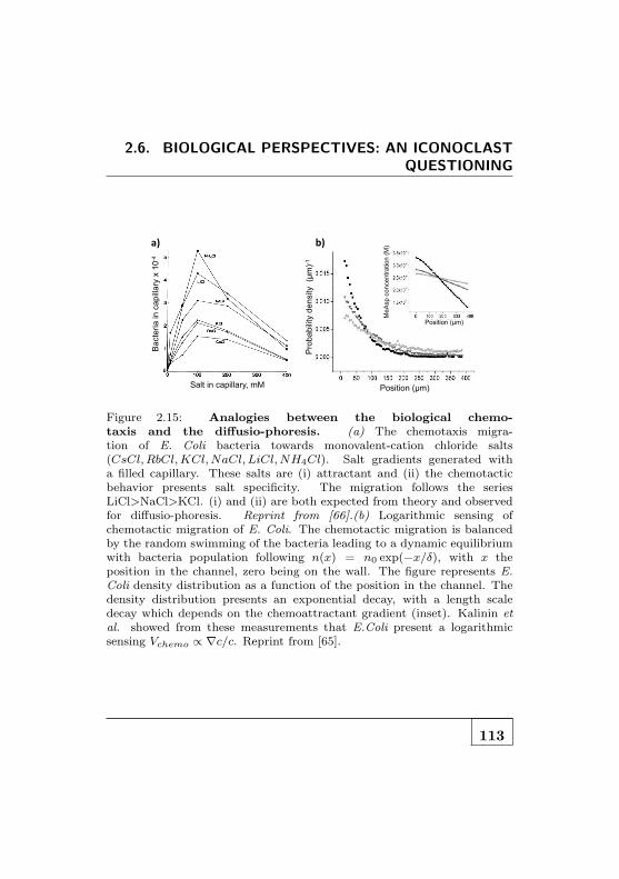
2.6. BIOLOGICAL PERSPECTIVES: AN ICONOCLAST
QUESTIONING
Salt in capillary, mM
Bacte
ria
in c
apill
ary
x 1
0-4
Position (!m)
Pro
babili
ty d
ensity
(!m
)-1
Position (!m)
MeA
sp
concentr
ation (
M) !"# $"#
Figure 2.15: Analogies between the biological chemo-taxis and the diffusio-phoresis. (a) The chemotaxis migra-tion of E. Coli bacteria towards monovalent-cation chloride salts(CsCl,RbCl,KCl,NaCl, LiCl,NH4Cl). Salt gradients generated witha filled capillary. These salts are (i) attractant and (ii) the chemotacticbehavior presents salt specificity. The migration follows the seriesLiCl>NaCl>KCl. (i) and (ii) are both expected from theory and observedfor diffusio-phoresis. Reprint from [66].(b) Logarithmic sensing ofchemotactic migration of E. Coli. The chemotactic migration is balancedby the random swimming of the bacteria leading to a dynamic equilibriumwith bacteria population following n(x) = n0 exp(−x/δ), with x theposition in the channel, zero being on the wall. The figure represents E.Coli density distribution as a function of the position in the channel. Thedensity distribution presents an exponential decay, with a length scaledecay which depends on the chemoattractant gradient (inset). Kalinin etal. showed from these measurements that E.Coli present a logarithmicsensing Vchemo ∝ ∇c/c. Reprint from [65].
113

CHAPTER 2. DIFFUSIO-PHORESIS IN A CONTROLLED
GRADIENT : A GEL DEVICE
within the body. Position within the body is coded by spe-cific gene expressions programs and affects cell’s differenciationand functional characteristics [67]. For successfull cytokinesis,i.e. the last step of the cell cycle with physical separation intotwo daughter cells, it is crucial to place the cleavage furrowin the right place between the separated chromosones, at thecell equator, task performed by actin cytoskeleton [68]. Thetranscription to proteins is regulated in animal cells by the in-tracellular localization of RNAs [69]. And bacteria control theircellular anatomy through the intracellular location of individ-ual proteins during growth and division in response to externalstimuli [70].These examples demonstrate the key role played by spatial or-ganization in biological systems and this domain has been veryactive over the recent years. In this context, concentration gra-dients of species, namely morphogens, are of prime importancein the toolbox of living systems and provide readily sophisticatedfunctionalities associated with spatial signaling, localization andpattern formation [71]. In order to figure out the positional in-formation given by a concentration gradient, we consider a 1Dcell for the sake of simplicity. A biological process, not definedhere, imposes a smooth gradient of a morphogen A in the cell,with high concentration on one pole and low concentration ofA on the other pole. We consider a gene B which is expressedin B∗ presence of A, A is the activator of the B gene. Thesmooth gradient of A is translated, by threshold effect relatedto the activation kinetics, into a sharp boundary of B∗ leadingto varying expressions of a gene in the cell, i.e. spatial organi-zation in a cell ! Structural patterns thus have their origins in
114

2.6. BIOLOGICAL PERSPECTIVES: AN ICONOCLAST
QUESTIONING
spatial patterns of morphogen molecules both at intra or supra-cellular level.
At the supra-cell level.The primary determinant of patterning along the anterior-posterioraxis in the fly Drosophilia is the gradient of the Bicoid (Bcd)morphogen, established by maternal displacement of Bcd RNAat the anterior end of the embryo. Bcd regulates genes ex-pressions which generates a reproducible spatial patterns [72].Similar mechanism with BMP morphogens are also reported inthe dorsal region of Drosophilia embryos [73].
At the intra-cellular cell level.In the bacterium E. Coli, the Min19 proteins oscillate betweenthe cell poles to select the cell center as division site by reaction-diffusion type mechanism. Furthermore, the same proteins spon-taneously form spatial planar surface waves on a flat membranein vitro with only limited number of proteins (MinD and MinE),ATP and a membrane. It underlines how complex behavior canemerge from strongly non-linear reaction-diffusion dynamics de-spite a small number of components at use [74]. Alternatively,the cell polarity protein Pom1 localized at the cell end regulatesa signaling network that contributes to the control of mitoticentry at the beginning of the cell division [75]. Morphogen gra-dients are at the core of the location of the cell division planefor bacteria [70, 76, 77]. Mathematically the emergence of spa-
19Min is a family of proteins. Here the system consists of proteins MinC,MinD and MinE.
115
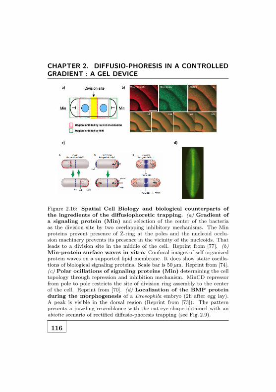
CHAPTER 2. DIFFUSIO-PHORESIS IN A CONTROLLED
GRADIENT : A GEL DEVICE
!"#$"#
%"# &"#
Figure 2.16: Spatial Cell Biology and biological counterparts ofthe ingredients of the diffusiophoretic trapping. (a) Gradient ofa signaling protein (Min) and selection of the center of the bacteriaas the division site by two overlapping inhibitory mechanisms. The Minproteins prevent presence of Z-ring at the poles and the nucleoid occlu-sion machinery prevents its presence in the vicinity of the nucleoids. Thatleads to a division site in the middle of the cell. Reprint from [77]. (b)Min-protein surface waves in vitro. Confocal images of self-organizedprotein waves on a supported lipid membrane. It does show static oscilla-tions of biological signaling proteins. Scale bar is 50µm. Reprint from [74].(c) Polar ocillations of signaling proteins (Min) determining the celltopology through repression and inhibition mechanism. MinCD repressorfrom pole to pole restricts the site of division ring assembly to the centerof the cell. Reprint from [70]. (d) Localization of the BMP proteinduring the morphogenesis of a Drosophila embryo (2h after egg lay).A peak is visible in the dorsal region (Reprint from [73]). The patternpresents a puzzling resemblance with the cat-eye shape obtained with anabiotic scenario of rectified diffusio-phoresis trapping (see Fig. 2.9).
116

2.6. BIOLOGICAL PERSPECTIVES: AN ICONOCLAST
QUESTIONING
tial patterns relies in a strong non-linearity in the evolutionequation of the system and its components. In the context ofspatial cell biology, various feedback mechanisms have been pro-posed, all supported by reaction-diffusion equation in a Turinglike approach [78]. The biological system presents sources andsinks of various signaling protein [77, 79] leading to a gradient(see Fig. 2.16-a). Other species are inhibited or expressed bythe presence of signaling proteins leading to the emergence ofpatterns. Thanks to the non-linearity of the chemical reactionkinetics and the coupling of a large number of these complexequations involving many intermediate chemicals, various pat-terns can be achieved and a good agreement between experi-mental and numerical predictions are achieved [73,80].This makes diffusion-reaction approach the “standard” descrip-tion of self organization in biological systems. Nevertheless theprecise positioning mechanism remains elusive and still raisesmany questions, concerning the building-up of the gradientsthemselves [81] and the process by which these gradients areread by the organizing entities. Also the accuracy and robust-ness of the positioning mechanisms especially in the noisy en-vironment of biological systems remain puzzling [72]. Finallyspatial cell biology strongly relates patterning mechanisms withconcentration gradient of species, the morphogens. In this con-text, we address the question of the potential role of the diffusio-phoretic trapping mechanism we unveiled –trapping by rectifiedoscillations and osmotic shock– in the spatial organization ofbiological systems. Again this question is very iconoclastic butdeserves to be raised.
117

CHAPTER 2. DIFFUSIO-PHORESIS IN A CONTROLLED
GRADIENT : A GEL DEVICE
Q3: Could the diffusio-phoretic patterning mechanismsplay any role in the spatial organization of biologicalsystems?This questioning is mainly speculative and we can not makeclear statement on the role played by diffusio-phoresis in spa-tial cell biology. But some characteristics of the physical phe-nomenon further support its potential relevance in biological en-vironment. As main point, diffusio-phoresis is sensitive to van-ishing concentration gradients, quite compatible with biologicalmorphogens concentrations, typically µM. Moreover, as a sideremark, the spatial extension of the diffusio-phoretic trapping isproportionnal to the length scale of the gradient (see equation2.8). Patterning can thus be achieved at the scale of a singlecell bacterium or during morphogenesis on much larger scale.Actually they are cons and pro for the possible role of diffusio-phoresis in these systems:
Cons:Spatial cell biology is strongly specific, e.g. only very specificgenes are spatially expressed in a morphogen gradient, and pro-teins react only to specific markers, by key-lock interaction. Bycontrast diffusio-phoresis is very generic and the phenomenontakes place each time the particle surface interacts with the so-lute through the interaction potential U . But this argument canbe partially answered if the potential U is itself very specific, i.e.requires specific interaction between the morphogen and the bi-ological particle.
Pros:
118

2.6. BIOLOGICAL PERSPECTIVES: AN ICONOCLAST
QUESTIONING
1. Biological systems present concentration gradients of mor-phogens in which biological colloids –proteins– should mi-grate by diffusio-phoresis.
2. Temporal oscillations of concentration occur in many ex-perimental systems: Min proteins concentration oscillatesfrom pole to pole in cell which is crucial to determinethe cell topology and define the equator as the divisionsite. (see Fig. 2.16-c), [74]. Moreover, pH as well as Ca2+
gradients oscillations are observed in pollen tubes, even ifthe mechanisms underlying the oscillations as well as theirphysiological role remain unknown [82].
Several biological systems present all the necessary ingredientsfor a diffusio-phoretic migration and possibly the localizationof species induced by concentration oscillations. Nonethelessanswering the question deserves a complete and specific studywhich has not been done up to now.Finally, given the robustness of diffusio-phoresis mechanism, itis interesting to go reverse and ask the following -open- questionas a conclusion of this section on the role of diffusio-phoresis inthe context of spatial cell biology:
All the ingredients being present, why would diffusio-phoresis not play any role in biological systems?
119

CHAPTER 2. DIFFUSIO-PHORESIS IN A CONTROLLED
GRADIENT : A GEL DEVICE
In this chapter, I studied diffusio-phoresis with colloidsor biological macromolecules in a controlled concentra-tion gradient which required the development of hydro-gel microfluidics. I characterized the diffusio-phoreticmigration of the particles and measured –in agreementwith theoretical predictions– a diffusio-phoretic velocityin electrolyte gradients:
VDP ∝ ∇ log c
I demonstrated experimentally that patterning of parti-cles arise from the logarithmic sensing. The non-linearityof the expression leads to (i) trapping of particles by rec-tification of oscillations while the high sensibility to van-ishing concentrations of the log-sensing is harnessed toobtain (ii) particles segregation by osmotic shock. Theobservations are rationalized by theoretical and numeri-cal predictions. Finally, I discussed further perspectivesof diffusio-phoresis and arose an iconoclast questioningof the relevance of the phenomenon in biology.
The big picture
120

2.7. APPENDICES
2.7 Appendices
Appendix A: Soft Lithography of Microflu-
idic Masks
The design and realisation of the silicon mold are based on stan-dard soft lithography techniques. I will consequently briefly re-port the steps and the interested reader can refer to [83, 84] tolearn more on the art of microfabrication.The desired features are designed on Adobe Illustrator R©(seeFig. 2.2) and printed at 3600 dpi on transparent films (APOLyon). The microfabrication is performed at the INL (Insti-tute of Nanotechnology Lyon) clean room. The positive relieffeatures on the silicon mask are obtained with a SU8 perma-nent epoxy negative photoresist (SU8-2100, Microchem). Theexperimental parameter are adaptated from the standard pro-cessing guideline to obtain channels of ∼ 120µm thickness inour facilities [85]. The following steps of lithography with theirparameters are the following.
1. Dehydration and Silicon Etching. A 4 inch diametersilicon wafer is first dehydrated on a hotplate at 200Cfor 30′ and cleaned with a plasma etching (RIE 51 MRC)at 200mTorr with 02 during 2′30”. The oxygen plasmais used to clean the silicon surface by reacting with theorganic residues. The resulting volatile products are sweptaway by the pumping action of the vacuum.
121
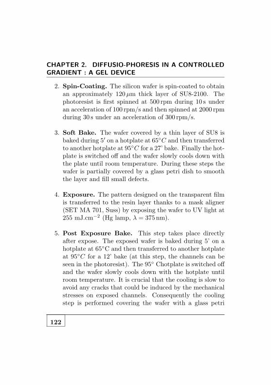
CHAPTER 2. DIFFUSIO-PHORESIS IN A CONTROLLED
GRADIENT : A GEL DEVICE
2. Spin-Coating. The silicon wafer is spin-coated to obtainan approximately 120µm thick layer of SU8-2100. Thephotoresist is first spinned at 500 rpm during 10 s underan acceleration of 100 rpm/s and then spinned at 2000 rpmduring 30 s under an acceleration of 300 rpm/s.
3. Soft Bake. The wafer covered by a thin layer of SU8 isbaked during 5′ on a hotplate at 65C and then transferredto another hotplate at 95C for a 27’ bake. Finally the hot-plate is switched off and the wafer slowly cools down withthe plate until room temperature. During these steps thewafer is partially covered by a glass petri dish to smooththe layer and fill small defects.
4. Exposure. The pattern designed on the transparent filmis transferred to the resin layer thanks to a mask aligner(SET MA 701, Suss) by exposing the wafer to UV light at255 mJ.cm−2 (Hg lamp, λ = 375 nm).
5. Post Exposure Bake. This step takes place directlyafter expose. The exposed wafer is baked during 5’ on ahotplate at 65C and then transferred to another hotplateat 95C for a 12’ bake (at this step, the channels can beseen in the photoresist). The 95 Chotplate is switched offand the wafer slowly cools down with the hotplate untilroom temperature. It is crucial that the cooling is slow toavoid any cracks that could be induced by the mechanicalstresses on exposed channels. Consequently the coolingstep is performed covering the wafer with a glass petri
122

2.7. APPENDICES
dish and preferentially on a hotplate with high thermalinertia. The cooling time is typically 2 h.
6. Development. The wafer is immersed in a developmentsolution of PGMEA, vigorously agitated during 30′ andthen rinced with acetone and ethanol. If a thin film ofphotoresist remains on the wafer or between the channel,this development step is repeated until removal of all non-reticulated photoresist.
7. Hard Bake. We make a post hard-bake procedure onthe mask to strengthen the mechanical properties of theSU8 and its adhesion on the silicon wafer given the thermalcycles imposed by the molding process. The mask is bakedat 150C during 1 − 2 h and let cool on the switch offhotplate during a couple of hours.
123

CHAPTER 2. DIFFUSIO-PHORESIS IN A CONTROLLED
GRADIENT : A GEL DEVICE
Appendix B: Hydrogel Microfluidic Chan-
nels
Hydrogel preparation
Agarose hydrogel powder (Agarose ME, for biochemistry, Acros)is weighted with a precision balance and added to ultra-purewater (resistivity 18.2 MΩ, MilliQ) up to a 4.5−5% w/v solution.This concentration is much higher that what biologist usuallyuse for cell cultures and presents a good compromise for both agood mechanical response after settling of the gel (high enoughYoung modulus, good stiffness) and a low enough viscosity andaging time of the liquid phase essential for the molding step.The solution is vortexed 30 s and appears as a cloudy suspension.It is microwaved at maximum power in a 50ml centrifugatingtube during ∼ 30 s until boiling. The solution is then shakedand microwaved again for five additionnal seconds. After theseheating steps, the agarose powder is fully dissolved in water andthe solution is homogeneous and transparent. Otherwise thesolution is shaken and microwaved again. The liquid hydrogel ispoured in a beaker on a hotplate at 80−90C and gently stirredat typically 100 − 200 rpm. The magnetic stirrer is necessaryto ensure a good thermal homogeneity in such a highly viscoussolution but must not inject bubbles in the hydrogel. The beakeris covered to limit evaporation and settling at the surface untilsubsequent use and molding of hydrogel channels.
124

2.7. APPENDICES
Agarose gel microchannels
The silicon master is placed on a hotplate at 75C. A volume ofhot liquid agarose typically 1.5− 2ml is poured onto the mold.The silicon wafer is then removed from the hotplate . Then aplexiglas manifod with a PDMS spacer (item 2 of figure 2.17) ispressed onto the mask. The PDMS spacer is a rectangular ringof thickness ∼ 700µm higher than the depth of the channels (∼ 120µm) and defines the shape and the thickness of the gelstamp. The agarose gel covered by the manifold is cooled atroom temperature during 40−60 s until settling of the hydrogelmatrix. The agarose stamp is carefully peeled off the mask andstored in ultra-pure water at 6 C until subsequent use. Theinlets and outlets of the channels are holed with a metal tipprior to any use of the agarose stamp.
125

CHAPTER 2. DIFFUSIO-PHORESIS IN A CONTROLLED
GRADIENT : A GEL DEVICE
Appendix C: Running an experiment, step
by step
Assembly of the device, filling of the microflu-idic chambers
!" #" $"
Figure 2.17: Photograph of the microfluidic device developed forthe gel system. Item-1 is the metal framework. Item-2 is the plexiglasmanifold to support the agarose stamp. Item-3 is the plexiglas cover of thesystem and ensures a proper sealing of the system.
The traditionnal sealing for PDMS soft lithography tech-niques is based on the covalent bonding of plasma activatedglass coverslip and PDMS microchannels. Such a covalent seal-
126

2.7. APPENDICES
ing cannot be achieved with hydrogel channels on a cover slipand we therefore developed a microfluidic device to seal agarosechannels on coverslips thanks to the applied pressure. A cleancoverslip of thickness 130 − 170µm is placed on a aluminiumframework (item-1, see Fig. 2.17)20. A recently holed agarosestamp is placed in the PDMS spacer frame of the plexiglasmanifold (item-2, see Fig. 2.17) with the channels opposite tothe plexiglas side. The plexiglas manifold is then inserted inthe plexiglas cover (item-3, see Fig. 2.17) with the channels op-posite to the plexiglas screw unscrewed (item 3’) Particles areintroduced in central chambers prior to the beginning of theexperiment because microfluidic chambers do not have inlet oroutlets. A large drop (∼ 1− 2ml) of the colloidal solution is de-posited on the clean glass slide. The item 3’ is tightly bound tothe metal framework (item 1) thanks to 4 screws driven in the4 cylindric blocks of the metal frame. The colloidal drop is thenpressed and one has to avoid capturing bubbles in the microflu-idic chamber while bubbles in the side channels will be expelledby the syringe-pump. Finally, the plexiglas screw is snuggedup until the applied necessary torque strongly increases due tothe contact of the PDMS frame-microchannels on the coverslip.We let the system relax for a few minutes. The system is thentightly sealed without any leakage!
20Different designs of this framework were manufactured to adapt vari-ous objectives. Indeed some objectives -in particular with high numericalaperture- have a working distance much shorter than the average metalthickness necessary to maintain the planarity essential for an efficient seal-ing of the device. The metal frame was therefore machined to allow closeapproach of the objective to the cover-slip
127

CHAPTER 2. DIFFUSIO-PHORESIS IN A CONTROLLED
GRADIENT : A GEL DEVICE
Microfluidic chambers and temporally tunablegradients
The microfluidic device described in the previous section is readyto be used and can be completed by microfluidic inlets and out-lets. The side-channels, used to impose the salt concentrationboundary condition in the system, are filled with a double sy-ringe pump (Kd Scientific) at a flow rate of Q = 0.1ml/minby means of 5ml plastic syringes (Braun) 21. Each syringe isfilled up with the buffer solution or 100mM salt (LiCl, NaCl orKCl) in buffer solution. Salt molecules diffuse freely in the pat-terned agarose gel while the solid hydrogel matrix prevents fromconvective flow between channels. Pressure differences in sidechannel and Darcy’s permeability of hydrogel walls makes fornegligible transverse flows as checked experimentally. Overall,side channels thus allows to set a concentration boundary con-dition, and the transverse gradient of salt in the central channelis linear and solution of the steady diffusion equation ∆c = 0(see Fig. 2.2-b). Temporal control is achieved with a manualmicrofludic switch (V140D, Upchurch) to reverse the concentra-tion boundary conditions. Finally, we used two types of motileparticles: polystyren-carboxylated fluorescent colloids (F8888200 nm, Molecular Probes, 2% w/v), diluted 10 times in Tris
21Note that the use of glass syringes systematically induces uncontrolleddissymetry between the channels and top-bottom bias in the chamber. Itis therefore necessary to use plastic syringes.The plastic syringes probablydeform to compensate the differences of heigth (and therefore pressure ap-plied at a given flux) between the 2 side channels which is precluded withthe much rigid glass syringes.
128

2.7. APPENDICES
buffer (1mM Trizma, pH9), and fluorescent phage-λ DNA (48kbp, Fermentas, Germany) at a concentration of 0.9nM in Tris-EDTA buffer (1mM Tris, 0.1mM EDTA, pH7.6).All the observations were carried out with an inverted micro-scope (DMI4000B, Leica R©) and a fluorescence camera (Orca,Hamamatsu R©). The fluorescence signal is recorded with a 20xobjective (ELWD, corrected for glass 0-2mm, N.A.0.4, 11506204,Leica) at 0.1Hz.
Appendix D: 1D concentration profile dur-
ing an osmotic shock
Calculations of the salt concentration profile are more transpar-ent in 1D, with a system confined in the interval |x| < ℓ/2.
c(x, t) =∑
k
ak e−Kkt cos((2k + 1)
π
ℓx)
2.28
with Kn = Ds
(
nπℓ
)2.
The initial condition is such that c(x, t = 0) = c0 for |x| <ℓ/2. One uses the identity:
c(x, 0) =4
π
∞∑
k=0
1
2k + 1(−1)k cos((2k + 1)
π
ℓx)
2.29
This leads to
c(x, t) =4
π
∞∑
k=0
1
2k + 1(−1)ke−Kkt cos((2k + 1)
π
ℓx)
2.30
129


Une face double, un charmant Janus, et, au-
dessus, la devise de la maison: ”Ne vous y fiez
pas”
A. Camus, La Chute 3Janus microswimmers
The collective behavior of self-propelled entities has raised con-siderable interest over the recent years in the context of non-equilibrium statistical physics [86–91]. Assemblies of active el-ements are rather commonly encountered in “societies” of bio-logical organisms and encompass systems as diverse -notably inscale- as swimming cells and bacteria colonies [92–99] , flocks ofbirds or sheeps and schools of fishes [87, 100]. All these entitiesmove actively by consuming energy and their behavior is thusintrinsically out of equilibrium. Building a general frameworkdescribing their collective properties remains accordingly a chal-lenging task and has led to a considerable amount of theoreticalwork along these lines [86–91,101]. By contrast, much less workhas been performed on the experimental side, and mainly onassemblies of living micro-organisms – which are naturally self-propelled – [92–96, 98, 99, 102–104] however at the expense ofa lack of control and flexibility of the individual particles and
131

CHAPTER 3. JANUS MICROSWIMMERS
their interactions. There is therefore a need to develop new ex-periments based on artificial model systems, involving suspen-sions of microscopic active particles with controlled propulsionand interaction mechanisms? Several routes to design individ-ual artificial microscopic swimmers have been explored in recentyears [105–109], taking advantage of the recent progresses madeto shape and design colloidal particles at microscales. Howevergoing from the individual to the many particles situation re-mains a challenging task and has not been achieved up to nowwith artificial motile particles.
Aim of this work
We aim at studying the properties of active matter, i.e. withactive particles, and the additional degrees of freedom givenby out-of-equilibrium phenomena over equilibrium paradigms.This out-of-equilibrium nature of the system leads to a rich vari-ety of new phenomena: collective behaviors, pattern emergence,break-down of the second principle ... We address this problemusing artificial diffusio-phoretic swimmers, namely Janus col-loids. The idea is to generate a solute gradient on the particleitself which in turn leads to a motion via diffusio-phoresis. Thisis done by means of a non uniform chemical activity on the par-ticle surface. Here we will follow a route proposed by proposedby Howse et al. [108]. And use the dismutation of hydrogen per-oxyde H2O2 on platinum catalyst asymmetrically coated on thecolloid. These particles convert the free energy into propulsionby diffusio-phoresis and provide synthetic “toy-models” in thestudy of the out-of-equilibrium properties of self-propelled par-
132

ticles (SPP). Moreover “chemical swimmers” interact throughhydrodynamic fields but also via the non-local concentration-field gradients they generate by the chemical reaction [110] andcould a priori present richer behaviors than simple SPP. Theconsequences of the chemical coupling with active systems havenot been considered up to now in the literature and appears asa relevant path to study collective behaviors out-of-equilibrium.
Organization of the chapter
I will first present the basics of life at low Reynolds number.This general part will describe the specificity of the dynam-ics of microorganisms and micro-swimmers and review a fewswimming strategies developed to overcome the time reversibil-ity of Stokes equation. In particular I will briefly review thecase of bio-mimetic synthetic swimmers. I will then introduce“phoretic” swimmers driven by interfacial motor and notablychemical Janus colloids, the core of the present work. I willreport the first results obtained by Howse et al. with these sys-tems in the “infinitely dilute”.To go further and study more concentrated regimes and ulti-mately collective effects, I developed improvements of the Janussynthesis. In a first step, I will characterize the high speed dy-namics of individual swimmers and show that it is a persistentrandom walk. Then, in the same spirit as the equilibrium statis-tical physics, I will turn to the response of a dilute assembly ofactive colloids under force field through a sedimentation experi-ment. I will show that in the “semi-dilute” regime, the system isproperly described as an equilibrium ideal gas of hot colloids at
133

CHAPTER 3. JANUS MICROSWIMMERS
temperature Teff , related to the energy injection by activity inthe system. This experiment is to my knowledge the only exper-imental measurement of effective temperature of active systems.Note that the experimental description of the synthesis of large collec-
tions of Janus colloids as well as benchmark experiments are gathered
for clarity in appendices A-C at the end of the chapter.
3.1 The harsh life of swimmers at low
Reynolds
Swimming microorganisms are ubiquitous in our world: algaeswim in oceans before feeding whales, bacteria travel in our guts,and spermatozoa are challengers during the fertilization race...But one has to keep in mind that the strategies developed by allthese microswimmers are very far from macro swimming tech-niques. The frontier between these two “worlds” is related tothe Reynolds number, Re ≡ UL/ν which compares inertial andviscous forces (U and L characteristic velocity and length scalesof the swimmer, respectively and ν the dynamic viscosity ofthe medium). While we experience at the human scale highReynolds number, typically 106 in a swimming pool or duringa sprint, a micron-size bacterium moving in water at 10µm/s,will present a Reynolds number of Re = 10−5. The world ofmicroorganisms is the world of low Reynolds numbers.In this world, the inertia does not play any role and viscousdamping dominates. It can be exemplified by the following sit-uation extracted from the famous paper by Purcell [111]. Let us
134

3.1. THE HARSH LIFE OF SWIMMERS AT LOW
REYNOLDS
imagine that we push a 1µm bacterium by a force f to move itat 30µm/s. Suddenly, we stop pushing and we wonder how farwill it coast before it slows down. Solving the equation of mo-tion with Stokes drag as the only force allows to answer -easily-the question. The bacterium moves 0.01 nm and the transienttime before stoppage lasts 0.6µs! At low Reynolds a microor-ganism experiences only the forces exerted and its dynamicsdoesn’t not present any inertial memory of the past. In otherwords, the Newton’s law becomes a simple statement of instan-taneous balance between external and fluid forces and torques.Any attempt to move by imparting momentum to the fluid as ina breaststroke is doomed and microorganisms need to developalternative strategies to overcome and exploit drag.
3.1.1 The scallop theorem.
Generally speaking, the flow field u and the pressure p in thesurrounding, incompressible and newtonian of with viscosity η,of a swimming organism is given by the Navier-Stokes equationwith the appropriate boundary conditions. At low Reynolds,this non-linear equation is reduced to the Stokes equation:
−∇p+ η∇2u = 0 with ∇.u = 0
3.1
This equation is linear and independent of time. As a conse-quence it presents a kinematic reversibility. Consider the motionof a solid body with an instantaneous prescribed velocity U androtation rate Ω together with the flow fluid surrounding it. Ifwe apply the scaling U → αU and Ω → αΩ, then by linear-ity the entire flow and pressure field transform as u → αu and
135

CHAPTER 3. JANUS MICROSWIMMERS
a) c)
b) d)
Figure 3.1: Theoritical swimmers with two discrete degrees of free-dom. (a) Purcell’s swimmer. Original drawing of Purcell’s swim-mer constituted of three linked rods. The sequence of motion is rep-resented through 5 different conformations to make a non-reciprocal cy-cle. (b) Macroscopic realization of a Purcell’s swimmer. Extractedfrom [112] and photo courtesy of Brian Chan and Peko Hosoi. (c) Three-spheres low reynolds swimmers proposed by Najafi et al.. Red arrowsindicate change of conformation of the swimmer shape. Thanks to the2 degrees of freedom, the cycle breaks the time-reversible symmetry andmakes a non reciprocal sequence of shapes. Reprint from [112]. (d) Ex-perimental realization of a micropump with colloidal beads andoptical tweezers following the route proposed for the three-sphere swim-mers. Reprint from [113].
136

3.1. THE HARSH LIFE OF SWIMMERS AT LOW
REYNOLDS
p → αp. The instantaneous flow streamlines thus remain iden-tical and the fluid stresses undergo a linear scaling, resulting inthe symmetry F → αF and Ω → αΩ, the force and the torquerespectively, acting on the body. In particular, when α = −1,an instantaneous reversing of the forcing does not modify theflow patterns, but only reverse its direction [112]. In short, atlow Reynolds, time makes no difference and only changes in theconformation of the swimmer matter. This result has two con-sequences. First, the rate independence : if a swimmer performsa sequence of shapes, the distance travelled by the swimmerdoes not depend on the rate at which the surface deformationoccur but only on the geometry of the configurations. The sec-ond main consequence is what is called the scallop theorem. Ifa swimmer performs a reciprocal motion, i.e. its body changesits shape and then goes back to the original shape by goingthrough the sequence in reverse, it does not move. Thanks tothe linearity and time independence underlined in Stokes equa-tion (Eq- 3.1), fast or slow, the “swimmer” retraces exactly itstrajectory. For this reason, a scallop opening its shell slowly andclosing it fast squirting out water could not move if it lived atlow Reynolds! As well as any animal that would try to swim bya reciprocal motion1...
1Nevertheless one has to keep in mind that rate independence and scalloptheorem remain true only in newtonian fluids and/or for individual swim-mers. Hydrodynamic interactions between reciprocal swimmers can breakthe time-reversibility and lead to collective locomotion. Moreover the dy-namics of micro-swimmers in non-newtonian fluids like most biological onesis much more complex than in a newtonian fluid [114–116]. These situationsare beyond the scope of this brief introduction on low Reynolds dynamics
137

CHAPTER 3. JANUS MICROSWIMMERS
Figure 3.2: Cross-section of anaxonene from wild type Chlamy-domonas. The diameter is approxi-mately 200 nm. We can observe thenine peripheric and the central micro-tubules doublet separated by dyneinmotors. Courtesy of Steve King, ex-tracted from [112].
Consequently, only systemswith at least 2 degrees offreedom in the configurationspace can swim. The fa-mous “Purcell swimmer” isan hypothetic animal “like aboat with a rudder at bothfront and back and nothingelse” [111] (see Fig. 3.1-a). Itperforms a cycle in the con-figuration space and a netdisplacement in space. An-other theoretical swimmerwith 2 degrees of freedomwas proposed by Najafi et al.with a three-spheres swim-mer [117]. An experimentalrealization of this swimmer,based on the forced motionof three colloidal beads by optical trapping recently showed thesuccess of this system to generate flow [113]. Of course, Naturehad to face the specificity of low Reynolds motion much beforephysicists and and regarding these constraints microorganismsdeveloped in two classes: “corkscrew” and flexible swimmers.Corkscrew swimmers continuously rotate their flagella which
and will not be developed in this manuscript. They are mentioned to pointout that surprising situations can come up despite the apparent simplicityof Stokes equation.
138

3.1. THE HARSH LIFE OF SWIMMERS AT LOW
REYNOLDS
propels the swimmer. This strategy is used by spiroplasma bac-terium (see Fig. 3.3-c) which generates “kinks” to rotate its corkshape [118,119]. Alternatively,flexible swimmers present a flex-ible flagella acting like an oar. While a stiff oar only presentsone degree of freedom and can not propel, a flexible one willdeform and change its shape during the first and the secondhalf of the stroke leading to a non-reciprocal cycle. Eukaryoticorganisms with flexible flagella and cilia belong to this class ofswimmers. The beating is then actuated by a continuous distri-bution of molecular motors along the filament or axonene. Thecore of a eukaryotic flagellum consists in nine microtubules dou-blets spaced along the circumference of the flagellum, with twomicrotubules running along the center. The bending originatesin the relative sliding of neighboring microtubule doublets whilethe sliding is driven by dynein motors regularly spaced along themicrotubules (see Fig. 3.2). Non-reciprocal motion is not suffi-cient for multiflagellated of ciliated organisms, and synchroniza-tion of the beating filaments is needed to achieve propulsion. Inthat respect, the full dynamics of many biological systems goesfar beyond the actuation of beating flagella.
The study of these mechanisms is under intensive research,and recent studies underlined the importance of hydrodynamicsinteractions [120] and flow patterns [121] to couple the beatingmotors -up to thousands of cilia for Volvox [98]- and propel themicroorganisms. Nevertheless these results are far beyond thescope of this section -which is to give a general basic intuition ofthe completely different “way of life” experienced by swimmingmicro-organisms- and will not be developed here despite theirgreat interest.
139

CHAPTER 3. JANUS MICROSWIMMERS
a) b)
Figure 3.3: (a) Spiroplasma : a corskrew swimmer. “Kink” propaga-tion in change of handedness of the helix propels the bacterium in viscousfluids [118]. Extracted from the illustrated glossary of plant pathology. (b)Chlamydomonas, a flexible flagellated swimmer. The propulsion of theorganism relies on the time-reversibility breakage due to the flexibility ofthe flagella. The full dynamics of the organism relies on the complex syn-chronization of the beating flagella out of the scope of this manuscript [120].Photograph from the Kamiya Lab, University of Tokyo.
140

3.2. JANUS MICROSWIMMERS
3.2 Janus microswimmers
3.2.1 Artificial microswimmers
Besides the intense research to understand the fundamentalmechanisms –both in biological and physical perspectives– un-derlying the motion of living microorganisms, swimming at lowReynolds is a keystone in the race for miniaturization. Micro-robotics and microfluidics need autonomous artificial swimmersand motors to carry and perform tasks at small scales. Twodifferent paths have been explored in this quest: a biomimeticapproach or the use of interfacial “self-phoretic” phenomena.We consider the latter class of swimmers in this thesis.
Biomimetic swimmersThese synthetic swimmers mimic the surface distortion andswimming strategies that proved to be efficient in biologicalsystems. Such approach was successfully followed by Dreyfuset al. to produce magnetic artificial microswimmers [105]. Alinear chain of magnetic colloids constituted an artificial flagel-lum linked to a red blood cell, the head of the artificial organism.An oscillating transverse magnetic field induces a non-reciprocalbeating pattern of the colloidal filament mimicking spermatozoaand a net displacement of the so-called “swimmer”.
Interfacially-driven microswimmersAn alternative route is to take advantage of physical phenom-ena predominant at small scales, notably surface effects. Takingtheir origin in an interplay with the surface, “phoretic” effects
141

CHAPTER 3. JANUS MICROSWIMMERS
a) b)
Figure 3.4: Different strategies to develop synthetic microswim-mers.(a) Biomimetic approach. Like a spermatozoid, the microswimmer hasa head (red blood cell) and an tail (flexible magnetic filament). Filamentbeating is actuated by an oscillating magnetic field and propels the swim-mer. Scale bar is 5µm. Reprint from [105]. (b) Phoretic swimmers.A colloidal particle is driven under motion by the gradient of a field (redgradient on the sketch). The diffuse layer -close to the surface- (brownstroke) in a field gradient gives a slip velocity along the particle surfacewhich consequently moves (black arrow).
142

3.2. JANUS MICROSWIMMERS
present a natural path given the increased surface to volumeratio at small scales. As developed in the first part of thismanuscript, a gradient of a field (electric potential, temperature,concentration of solute) leads to the motion of particles thanksto interfacial phenomena (electrophoresis, thermophoresis, anddiffusio-phoresis respectively). In short, the diffuse nature ofthe charged interface leads to a slip velocity across the interfaceand flow generation (see [23] and chapter 1). Experiments suchas those we described in the previous chapter underlined therelevance of phoretic phenomena to generate flow and motionat microscale. Macro-molecules and colloids move along tem-perature gradient by thermophoresis [31,32] or along concentra-tion gradient by diffusio-phoresis [17]. Moreover, heterogeneousnanorods with various catalytic or chemical reactions at theirdifferent ends have been reported to propel despite the physicalmechanism at the origin of the propulsion remains debated: selfelectrophoresis [106, 122] or Marangoni effect [107]. The readerinterested in phoretic phenomena will find much complete de-velopments in chapter 1.
3.2.2 Janus microswimmers
Janus particles
Janus particles are colloid-sized particles with two hemispheresof different surface chemical composition. Thanks to the asym-metry of their hemispheres, Janus particles appear as properbuilding block for supraparticular assemblies. This idea was firstrestrained by the lack of synthetic methods. But in recent years,
143

CHAPTER 3. JANUS MICROSWIMMERS
important efforts were devoted to the development of chemicalengineering that allowed to provide access to particles with awide range of shape and materials, making synthesis of Januscolloids possible [123,124]. The technological stepforward foundapplications in domains as diverse as: solid surfactants followingthe original idea of De Gennes, ‘micro-shuttles” thanks to ICEOforces [8,125], or self assembly bricks [126,127] (see Fig. 3.5-a)...The interested reader can will find more informations about thesynthesis and additional experimental Janus particles in recentreviews [123,124].
Janus diffusio-phoretic microswimmers
Based on phoretic phenomena, Ajdari et al. proposed a sim-ple model for a microswimmer based on self-diffusio-phoresis[110, 128]. A colloid is driven by an asymmetric chemical ac-tivity taking place on its surface and a consequent gradient ofreaction products and reactants (see figure Fig. 3.5-b). In or-der to use the surrounding medium as an infinite reservoir anddo not consume the colloid, the chemical activity of the surfaceshould be catalytic. While Ajdari et al. addressed various andcomplex distributions of the chemical activity, we will focus onthe case of the Janus colloids, i.e. one half chemically activeand the other half bare. These Janus particles are conceptu-ally easier to consider and developed experimentally. As wellthey constitute the first piece of all the experimental work weperform on swimmers.
144
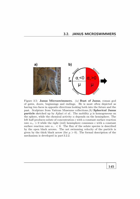
3.2. JANUS MICROSWIMMERS
a)
!+>0
"
z !=0
"
b)
!-<0 !
+>0
Figure 3.5: Janus Microswimmers. (a) Bust of Janus, roman godof gates, doors, beginnings and endings. He is most often depicted ashaving two faces in opposite directions looking both into the future and thepast. Sculpture from Vatican Museums collections.(b) Spherical Janusparticle sketched up by Ajdari et al.. The mobility µ is homogeneous onthe sphere, while the chemical activity α depends on the hemisphere. Theleft half produces solute of concentration c with a constant surface reactionrate α+ > 0 while the right (red) hemisphere consumes c with a constantsurface reaction rate α− < 0. The flux of the solute species is describedby the open black arrows. The net swimming velocity of the particle isgiven by the thick black arrow (for µ > 0). The formal description of themechanism is developed in part 3.2.2.
145

CHAPTER 3. JANUS MICROSWIMMERS
Diffusio-phoretic propulsion
Self-propelled colloids generate themselves the gradients of con-centration and move thanks to diffusio-phoresis. For the sakeof simplicity, we consider the simple situation of only one soluteat a given concentration c(rs), where rs is the considered posi-tion on the solid surface. The chemical activity is simplified ina consumption or creation of this species. The diffusio-phoreticvelocity is proportional to the gradient and yields to:
V = µ∇c
3.2
where µ is the so-called diffusio-phoretic mobility of the particle.At steady state, in the reference frame of the particle, and ne-glecting the effects of the motion of the colloid in the transportof the salt at small Peclet number [128] the solute concentrationis given by:
D∇2c = 0−Dn · ∇c(rs) = α(rs)
3.3
where D is the solute diffusion coefficient. α(rs) measures thechemical activity of the surface at position rs, e.g. the genera-tion or the consumption of the solute by the catalytic reactionon the surface. We assume for simplicity that α is a constant atgiven position on the surface, and only depends on the catalystpresent at this point2.
2A priori, the chemical activity is a complex quantity which dependson the number of available catalyst sites and on the concentration of soluteat a given position. As a consequence, our assumption is not obvious.
146

3.2. JANUS MICROSWIMMERS
The concentration gradient of Janus particles develops on theparticle size R and Eq- 3.2 thus rewrites dimensionaly V ∼µ∆c/R, where ∆c is the typical concentration difference be-tween the poles of the colloid and originates in the chemicalreaction. Using equation 3.3 dimensionally leads to a typicalpropulsion velocity:
V ∝ αµ/D
3.4
This expression underlines the importance of the competitionbetween the reaction rate α and the diffusivity D of the consid-ered solute to maintain a driving force via the solute gradient.Moreover, for a given pattern of surface properties and particleshape, the velocity of the self-propelled particle is independentof the swimmer size R. This result is quite different from thescaling of the velocity for an object propelled by a body forceF , e.g. gravity: the force F ∝ R3 is balanced by the Stokesviscous drag which leads to a velocity V ∝ R2. This pointemphasizes the robustness to downsizing of phoretic motor andnotably diffusio-phoresis for propulsion3.
Nevertheless if the solvent contains an excess of the reactants necessary toproduce or destroy the solute of interest, the density of active catalytic siteson the surface is what limits the reactions. In this case, α is reduced toa reaction rate constant per surface unit. α > 0 represents the number ofmolecules of the solute of interest generated at the surface per second andper surface unit [128]. In our case, the solution acts as an infinite reservoirand one can reasonably think that the chemical reaction on the catalyticsites limit the reaction. Anyway, this hypothesis allows to catch the physicsand the feeling of the phenomenon.
3The above description is especially derived in the case of self -diffusio-phoretic swimmers, but the general formalism is still valid for any phoreticphenomenon. A particle which autonomously generates an electric field
147

CHAPTER 3. JANUS MICROSWIMMERS
A full resolution of the previous equations can be performed be-yond the dimensional arguments. We consider chemical Januscolloids which generate autonomously the gradients of concen-tration via catalytic reactions on the two hemispheres. Theyare covered with two different catalytic materials with differentchemical activities α+ and α−. In general, the mobilities canalso differ for the speciess on each side and we note the µ+ andµ−. Ajdari et al. derived the full expression for the diffusio-phoretic velocity of the swimmer [110]:
V =1
8
1
D(α+ − α−)(µ+ + µ−)ez
3.5
This result once again pinpoints the importance of the symmetrybreaking in the chemical activity to propel the colloid.
Platinum-bare Janus microswimmers
Howse et al. proposed in a recent work a route to synthesize arti-ficial colloidal microswimmers [108]. Following the scheme pro-posed in the previous section and recent results of autonomousmotion of platinum-gold nanorods [106,129], he synthesized platinum-bare active colloids. One half of a commercial latex colloid iscoated by a thin layer (typically a few nm) of platinum while thesecond hemisphere of the colloid remains bare namely a Januscolloid (see figure Fig. 3.6-a).
Chemical reaction.
or thermal gradient will move along this gradient by, respectively self-electrophoresis or self-thermophoresis.
148

3.2. JANUS MICROSWIMMERS
Hydrogen peroxide H2O2 aqueous solution (in the range 0 to10% w/v) is added to the colloidal suspension of Janus parti-cles. While hydrogen peroxide is thermodynamically unstable,it does not dismute at room temperature. The kinetic block-age is passed if the hydrogen peroxide solution is put in contactwith an organic residue or any transition metal. The reductionof hydrogen peroxide then produces water and oxygen followingthe reaction:
2 H2O2 → O2 + 2H2O
Platinum-bare Janus particles thus present differential spatialchemical activity with hydrogen peroxide: the platinum side ofthe Janus catalyses the dismutation of H2O2 while the bare halfis chemically inert. With the notation of the previous part, thechemical activity on the platinum side is αPt = α 6= 0, and thechemical activity on the bare side is αb = 0.Finally, the particle presents on one side products of the reactionand on the other side a consumption of reactants. The chemicalsgradients propel the particle by self-diffusio-phoresis, accord-ingly to equation Eq- 3.5 and assuming equal diffusiophoreticmobility of the speciess µ+ = µ− = µ, the velocity (Eq- 3.5)rewrites as follows:
VDP =µ αPt
4D0
3.6
Note that additionally to the solute gradient, the chemical re-action may also induce a temperature gradient. The dismuta-tion reaction of hydrogen peroxide is indeed strongly exothermic(∆fH
0 = −188 kJ/mol) and local heating along the platinumhemisphere may induce a temperature gradient propelling the
149

CHAPTER 3. JANUS MICROSWIMMERS
colloid thanks to thermophoresis. In our experiments, the ap-parent velocity V is in a first approximation the sum of thedifferent phoretic velocities:
V = VDP + VT
3.7
where VDP is the diffusio-phoretic velocity of the particle in thesolute gradient generated by the chemical reaction and VT is thethermophoretic velocity of the particle in the thermal gradientgenerated by the exothermic dismutation. As our objective is tosynthesize artificial microswimmers, we do not try to separateand extract the different phoretic contributions of the particlesmotion and focus on the measurement of propulsion velocity Vdenoted as V in the following.Howse has demonstrated that the particles added in a solutionof “fuel” -H2O2- are propelled at a given velocity V whose am-plitude is controlled by the concentration of fuel accordingly toa Michaelis-Menten behavior for the decomposition of hydrogenperoxide on platinum [108]. The velocity first linearly increaseswith the fuel concentration and then tends to saturate (see fig-ure Fig 3.6-b) which can be interpreted as : (i) H2O2 forms acomplex [Pt(H2O2)] with rate per unit area k1[H2O2] and (ii)decomposes into water and oxygen with a rate per unit area k2independent of the peroxide concentration. Finally the effec-tive surface reaction rate α, defined on equation Eq- 3.5, can beexpressed as:
α = k2[H2O2]
[H2O2] + k2/k1
3.8
The parameters k1 and k2 can be extracted by fitting the veloc-ity dependence on hydrogen peroxide concentration and accord-
150

3.2. JANUS MICROSWIMMERS
ing to equation Eq- 3.6. This derivation presents a very goodagreement with experimental measurements (see Fig.3.6-b).
[H2O2] (%vol)
V (!
m/s
)
a) b)
Figure 3.6: (a) SEM picture of Janus, platinum-latex , colloids (scalebar 500nm) synthesized during my PhD. The platinum coating is 2 nm onone hemisphere of the colloid and appears bright on the picture. The con-trast is enhanced to enforce the brightness difference between the platinumand bare hemispheres. Grateful acknowledgments to J.M. Benoit. (b) Ve-locity measurements for platinum-bare Janus colloids (black) orbare colloids (red). They are obtained for various concentration of theH2O2 fuel (expressed in %/vol). The solid black line represents the fit ofthe velocity following a Michaelis-Menten kinetics for the dismutation ofhydrogen peroxide on platinum. Reprint from [108].
The first part of this chapter reported previous resultsin the literature on microswimmers, e.g. low Reynoldsnumber dynamics, Janus chemical microswimmers... Fromthis point, I will discuss now original contributions tothe field from my PhD work.
151
CHAPTER 3. JANUS MICROSWIMMERS
3.2.3 From individuals to larger collections ofmicroswimmers
In the present work, we followed the route proposed by Howseet al. to build microswimmers [108]. Our final aim is to studythe out-of-equilibrium properties of collectives of active self pro-pelled particles. This (i) requires to build up large collections ofJanus particles with “not too small” volume fraction –typicallyΦ ∼ 0.05 − 0.1%– which (ii) leads to some experimental diffi-culties.
Synthesizing large number of Janus particles
Inspired from the synthesis of Janus colloids proposed by Howseet al. I developed an improved protocol to strongly increasethe number of particles synthesized. A sufficient efficiency isrequired to obtain “concentrated” solutions of swimmers andexplore the physics of suspensions beyond the “infinitely dilute”regime. As the process is mainly technical, the detailed protocolof the synthesis of platinum-bare Janus colloids is displaced inAppendix C at the end of the chapter and I present here only asummary.A commercial solution of colloids is diluted –typically 200 times–in isopropanol and sonicated. A drop of the solution is depositedin a thin film on the rough side of a tilted 4′′ silicon wafer. Theroughness of the the substrate captures the contact line duringthe evaporation of the alcohol leading to an uniform dewetting ofthe film and the formation of a monolayer of individual colloids,i.e. without ring stains. A thin layer of platinum (typically
152

3.2. JANUS MICROSWIMMERS
2− 5 nm) is coated on the wafer by sputtering and one obtainsplatinum-bare Janus particles by shadowing effect. The parti-cles are resuspended in pure water by sonication of the waferand the solution is reconcentrated by centrifugation to finallyobtain a Janus suspension of ∼ 50µl with a maximal volumefraction Φ ∼ 0.1%.Nota Bene. The rough substrate prevents ring stains and dropletsformation and strongly increases the density of the monolayerof colloids. In addition with the use of large 4′′ substrate, thisexperimental protocol makes possible the synthesis of large col-lections of Janus particles.
Unlocking experimental difficulties: a gel device
“Concentrated” suspensions of Janus particles (with volume frac-tion in the range φ ∼ 0.01−0.1%) arise experimental difficulties.Large collections of swimmers (i) consume fuel -H2O2- and (ii)produce oxygen and oxygen bubbles which pollute the experi-ment. (i) can be verified experimentally monitoring the swim-ming velocity V along time checking that it remains constant4
during the experiment. But (ii) prescribes the use of glass cap-illaries or “traditional” enclosed systems as observation cells.The released oxygen exceeds solubility in the bulk and gas bub-bles appear. They strongly disturb measurements as they leadto fast recirculation flows and leakage.In order to unlock these experimental difficulties, I de-veloped a specifically designed microfluidic system based
4As pinpointed previously by Howse results, the amplitude of the propul-sion velocity is related to the fuel concentration in the bulk.
153

CHAPTER 3. JANUS MICROSWIMMERS
on a gel-microdevice technology allowing a constant re-newal of the chemical fuel, as well as removal of the waste, inan open reactor configuration.
A Gel microfluidic deviceThe swimmers are enclosed in a dedicated microfluidic devicemolded in agarose gel following the idea described in the pre-vious chapter and inspired by [44]. Let us remind that the hy-drogel nanoporous matrix acts as solid walls for the flow butallows free diffusion of molecules. The mold design is made of acircular microfluidic chamber and surrounded by two side chan-nels separated by gel walls (see Fig. 3.10-a). The central cham-ber is initially filled with Janus colloids in water, while H2O2
solution at concentration C0 is continuously circulated in lat-eral channels. This gel microsystem ensures a constant renewalof H2O2 fuel and removal of chemical waste products (O2) bydiffusion through hydrogel walls from the infinite reservoir andsink constitued by the circulating lateral channel. This providesa convection-free environnement5 in the colloids chamber withstable chemical conditions over hours, allowing to study largeassembly of active colloids. A similar study in a sealed capillarywould be limited to a few seconds by the production of oxygenbubbles. Unlocking the main experimental problems related tothe use of large collections of swimmers, we demonstrate therelevance of gel microfluidic tools to explore the properties ofactive colloidal suspensions.Nevertheless, the hydrogel technology presents specificities. H2O2
5With a typical drift V < 20 nm/s, see chapter 2.
154

3.3. MICROSWIMMER DYNAMICS: A PERSISTENT
RANDOM WALK
diffuses through the gel walls and alters the hydrogel structure.In order to quantify the consequences of the hydrogel aging, weperformed benchmarks experiments reported in the AppendixB of this chapter. The gathered results of the benchmark arereported on figure 3.7-b. The conclusions of these benchmarkexperiments can be summarized as:
1. After a few hours in contact with hydrogen peroxide, thediffusivity of the colloids reaches a plateau D0 = 0.34 ±0.02µm2/s independent of the H2O2 concentration andwhich remains stable up to 36 hours.
2. Beyond this time the degradation of the gel by H2O2 sys-tem is too strong to ensure good reliability of the system.
In the following experiments, we will inject H2O2 for a few hoursbefore measurements of the mean squared displacement to at-tain the “steady” viscosity and take D0 as the equilibrium valueof the diffusion coefficient of 1µm Janus colloids enclosed in gelmicrofluidic device.
3.3 Microswimmer dynamics: a persistent
random walk
We first characterize the individual dynamics of the active col-loids using high speed tracking measurements for proper tempo-ral resolution. While tracking the trajectories can be properlyperformed in a dilute sample from colloids films, we performsimultaneously sedimentation measurements (see next section).
155

CHAPTER 3. JANUS MICROSWIMMERS
0 20 40 600
0.1
0.2
0.3
0.4
0.5
!"#$
%&'()
*+$,)"-./0'() b) a)
!"##"$%&'
()#'
Figure 3.7: (a) Sketch of the gel microfluidic device. The design ismade of a circular microfluidic chamber surrounded by two side channelsseparated by gel walls. The central chamber is initially filled with Januscolloids in water, while H2O2 solution at concentration C0 is continuouslycirculated in lateral channels. This gel microsystem ensures a constantrenewal of H2O2 fuel and removal of chemical waste products (O2) bydiffusion through hydrogel walls from the infinite reservoir and sink con-stitued by the circulating lateral channel. This provides a convection-freeenvironnement to study mean squared displacements of colloids with highspeed camera. (b) Benchmark experiments on the effect of H2O2
on the gel device. We quantify the effect of H2O2 on the gel structurewith diffusion constants monitoring. The diffusion constants are extractedfrom mean squared displacements measurements at equilibrium for bare(blue) or Janus (red) colloids at. The diffusion coefficients measurementsare performed at different times, in water (open symbols) and H2O2 (fullsymbols). (⋆) is for an experiment in a glass capillary, the other experi-ments are performed with hydrogel systems. Black dashed lines representthe Stokes-Einstein equilibrium expectations DSE = 044 ± 0.02µm2/s.The measured diffusion constants agree with this value just after the in-troduction in the microfluidic chamber (glass or gel). It then decreasesto D0 = 034 ± 0.02µm2/s (magenta dashed line) with the introduction ofH2O2 and remains stable up to 2 days for various concentration of hydro-gen peroxide or in water. Beyond 2 days, the hydrogel presents aging andgets brittle. Measurements are then not reliable (grey zone).
156

3.3. MICROSWIMMER DYNAMICS: A PERSISTENT
RANDOM WALK
For this purpose, one has to handle “concentrated” solutions ofJanus particles (volume fraction φ ∼ 0.01%) which requires, asdiscussed above, the use of the gel microdevice.
3.3.1 Dynamics of microswimmers
Experimental protocol
Measurements of the dynamics of microswimmers are performedfor various H2O2 concentrations C0 (in the range 0 to 10%) ina circular microfluidic chamber (diameter Φ = 650µm, height≃80µm, volume V ≃ 30 nl) and surrounded by two side chan-nels separated by 125µm gel walls. The two-dimensional (x,y)motion of colloids is followed by fluorescent microscopy witha high speed camera (Phantom V5) at 100Hz and carried onan inverted microscope (DMI4000B, Leica) with a 60× objec-tive, water immersion and high numerical aperture (60x, WaterImmersion, N.A.=1.2, Nikon). The (2D) instantaneous colloidpositions r(t) are extracted from stack of images (typically 4000)with a single particle tracking algorithm (Spot Tracker, ImageJ [130]) to define the trajectories of the particles. As the ori-gin of the movie is arbitrary, we perform sliding time averageon the position denoted r(∆t) for a given time lag ∆t which is(i) the relevant observable and (ii) strongly increases the statis-tics of “short” times measurements. Finally, the mean squaredisplacement of the colloids at given fuel concentration C0 isobtained computing ∆L2(∆t) ≡ 〈(r(t+∆t)− r(t))2〉 where theaverage is performed over time for each individual trajectoryand then over an ensemble of trajectories denoted by 〈·〉. We
157

CHAPTER 3. JANUS MICROSWIMMERS
consider typically 20 independent particles which is sufficient fora statistical convergence.
Mean squared displacements
We plot in figure 3.8 ∆L2(t) as a function of time for bare (non-active) and active colloids in a solution of hydrogen peroxide,confirming the impact of injected chemical power on the indi-vidual motion of the colloids, in agreement with Ref. [108].
Equilibrium ExperimentsFor bare (non-active) colloids, the dynamics is purely diffusivei.e. the mean squared displacement is linear with time, andwe extract from the slope the diffusion coefficient of the colloid∆L2/4∆t = D0 = 0.34± 0.02µm2/s, which is found to be inde-pendent of the H2O2 concentration (see Fig. 3.7-b and AppendixB). We have furhermore measured the same value D0 for the dif-fusion coefficient of Janus colloids in pure water, at equilibrium,in the absence of H2O2 fuel. This value for the equilibrium dif-fusion coefficient of 1.1µm colloids is significantly smaller thanthe equilibrium Stokes Einstein value DSE = 0.44µm2/s withthe bulk water viscosity. As discussed above and in AppendixB, we infer that the difference is due to an increase of the viscos-ity of the hydrogen peroxide solution due to solubilized agarosegel.
Janus swimmersFor the Janus active colloids in a hydrogen peroxide solution,the mean square displacement differs drastically from the equi-
158

3.3. MICROSWIMMER DYNAMICS: A PERSISTENT
RANDOM WALK
(2 0 21(1(3 3
10(2
100
10(3
10(1
b)
PD
F
0 1 2 3 40
5
10
15
20
25
30
4D0
4Deff
a)
0 0.5 10
2
4
6
Figure 3.8: (a) Experimental mean squared displacements ∆L2(∆t)for bare (blue) and active colloids (red) in 7.5% H2O2 solution. Bare col-loids (bottom) show standard diffusion (∆L2 linear in time), while themean squared displacement of active colloids is fitted according to equa-tion (3.12). The measured diffusion coefficients are D0 = 0.33µm2/s forbare and Deff = 1.90µm2/s for active colloids. (Inset) Zoom of the meansquared displacement at short times scales. (b) PDF of particle dis-placement ∆R for various lag time ∆t as a function of the normalizeddisplacement ∆R/∆L(∆t). ∆t=0.3 s (⋆), 1 s (), 3 s (⋄) for bare (blue) andactive colloids (red) in a solution of 7.5% of H2O2. The dashed lines is thegaussian equilibrium prediction.
159

CHAPTER 3. JANUS MICROSWIMMERS
librium diffusive dynamics and strongly depends on the fuelconcentration. The colloid exhibits ballistic motion at shorttimes, ∆L2(t) ∼ V 2t2, while at longer times a diffusive regime,∆L2(t) ∼ 4Defft, is recovered with an effective diffusion coeffi-cient Deff much larger than the equilibrium coefficient D0.
A persistent random walkAs discussed in [108,131], the active colloids perform a persistentrandom walk, due to the competition between ballistic motionunder the locomotive power (with a constant swimming veloc-ity V ) and angular randomization by thermal rotational Brow-nian motion. The transition between the two regimes occurs atthe rotational diffusion time τr of the colloids. Physically, thistime scale represents the time for the direction of the particleto decorrelate. As the propulsion direction of a Janus swimmeris perpendicular to the equator of the colloid, τr also appears asthe time scale for which the direction of propulsion decorrelates.For t ≪ τr, the colloid propels along the direction u perpendic-ular to the equator and the rotational diffusion of the colloid isnegligible. The colloid goes along a straight line with velocity V.For t ∼ τr, a colloid crossed the distance V τr along u. Then thedirection of the propulsion is randomized and the colloid nowpropels along a new direction u′ decorrelated from the previousone. Finally, for t ≫ τr, the swimmer performs random steps oflength V τr with direction randomized at rate τ−1
r . Taking intoaccount the thermal diffusivity D0 of the colloid, the swimmerbehaves at long times as a Brownian particle with an effective
160
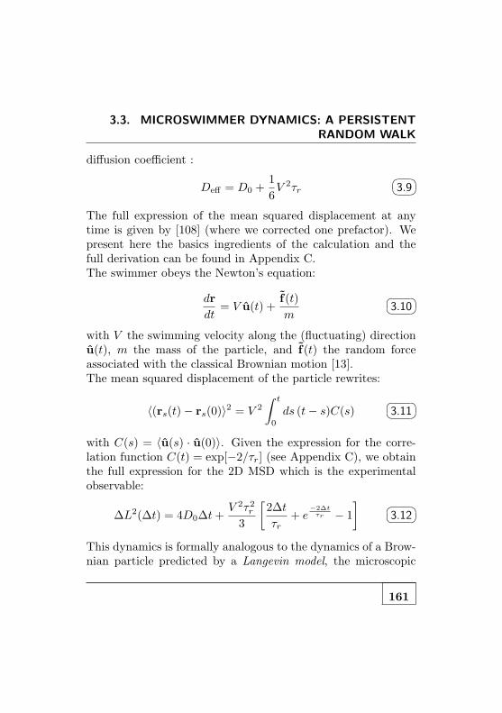
3.3. MICROSWIMMER DYNAMICS: A PERSISTENT
RANDOM WALK
diffusion coefficient :
Deff = D0 +1
6V 2τr
3.9
The full expression of the mean squared displacement at anytime is given by [108] (where we corrected one prefactor). Wepresent here the basics ingredients of the calculation and thefull derivation can be found in Appendix C.The swimmer obeys the Newton’s equation:
dr
dt= V u(t) +
f(t)
m
3.10
with V the swimming velocity along the (fluctuating) directionu(t), m the mass of the particle, and f(t) the random forceassociated with the classical Brownian motion [13].The mean squared displacement of the particle rewrites:
〈(rs(t)− rs(0)〉2 = V 2
∫ t
0
ds (t− s)C(s)
3.11
with C(s) = 〈u(s) · u(0)〉. Given the expression for the corre-lation function C(t) = exp[−2/τr] (see Appendix C), we obtainthe full expression for the 2D MSD which is the experimentalobservable:
∆L2(∆t) = 4D0∆t+V 2τ2r3
[
2∆t
τr+ e
−2∆tτr − 1
]
3.12
This dynamics is formally analogous to the dynamics of a Brow-nian particle predicted by a Langevin model, the microscopic
161

CHAPTER 3. JANUS MICROSWIMMERS
inertial time scale (∼ ns) being replaced by the rotational time(∼ s for 1µm colloids).
Back to the experimentWe fit the experimental mean squared displacement (MSD) ∆L2(∆t)using equation 3.12 with the propulsion velocity V as the onlyfitting parameter, while the value of D0 is taken from the equi-librium diffusion coefficient measured in water for Janus colloidsor in H2O2 for bare colloids. The rotational diffusion time τr isset at a constant value τr = 0.9 s in good agreement with Stokesexpectation τr = 8πηR3/kBT (for experiments with colloids ofradius R = 0.55µm at 25C in water η(25C) = 0.890mPa.s)6.As shown in Fig. 3.8-a, an excellent agreement with the experi-mental results is found with only one free parameter. The verygood fit lasts for times smaller than the rotational diffusion time∆t < τr as well as for times larger that this cut-off7.This supports the persistent random walk –with persistence timeτr and velocity V– to model the dynamics of microswimmers.Under the present conditions, we measure V in the range from0.5µm/s to 2.9µm/s. In terms of enhanced diffusion, the effec-tive diffusion constant Deff
8 can be increased by the swimming
6Nevertheless the fit is weakly sensitive on the precise value of τr in therange 0.8−1 s. As a consequence, we set the value to the Stokes equilibriumexpectation. The translational propulsion of the swimmer is not expectedto impact the angular balance between fluctuation and dissipation definingτr. This allows to use only one fitting parameter in equation 3.12.
7We also want to stress that we fit 400 data points with only one pa-rameter.
8Deff is obtained by measuring the slope in the linear region of theMSD i.e ∆t ≫ τr
162

3.3. MICROSWIMMER DYNAMICS: A PERSISTENT
RANDOM WALK
activity by a factor up to 5.5 compared to the equilibrium con-stant.In the following we use this measure of Deff as a probeof the colloidal “activity”.
Probability distribution functionWe can also extract from the trajectories of the colloids the prob-ability distribution function (PDF) of the displacement. To acertain extent the PDF is mainly a convenient way to rephraseprevious results with more sensitive statistical physics tools toprobe events like long time tails, intermittent dynamics... Wemeasure the PDF of the colloid displacement along x and y di-rections for a given time lag ∆t both for bare (blue) and active(red) colloid particles (see Fig.3.8-b). We check that (i) thePDF along x and y can be superimposed and (ii) are even withrespect to the zero axis for any time which ensures that there areno experimental bias! Finally, for both bare and active colloids,the PDF fits very well to a gaussian with variance ∆L2(∆t)given in equation 3.12.Although departures from a gaussian are expected at short timefor the persistent random walk, these are within experimentaluncertainty and we can not reasonably infer any specific outof equilibrium signatures from the PDF measurements. Indeed,more sophisticated theoretical predictions can also be performedon the dynamics of stochastic dynamics of diffusio-phoretic swim-mers. In particular, Golestanian identified three times scalesseparating four different regimes for Janus particles and showednon-markovian effects due to the diffusion of the chemical cloudand anomalous diffusion behaviors [132]. These long-time cor-
163

CHAPTER 3. JANUS MICROSWIMMERS
relations due to chemical relaxation are of premier importancefrom a fundamental point of view, nevertheless the experimen-tal validation of this result could be tricky: the contribution ofthese effects dominate at nm and ns in water and are robust tochange in the colloid size and only depends on the viscosity ofthe medium.To summarize, the active colloids are expected to per-form a persistent random walk of persistence time τrdue to the competition between ballistic motion underthe locomotive power (with a con- stant swimming ve-locity V), and angular randomization due to thermalrotational Brownian motion.
3.4 Sedimentation of active colloids
In the previous section we addressed and characterized the dy-namics of individual Janus particles and showed an out of equi-librium behavior of swimmers finally leading to an enhanceddiffusion coefficient Deff at long time-scale. The next step is tocharacterize the statistical behavior of an assembly of swimmers.Following a natural avenue in equilibrium statistical physics, wenow turn to the response of a collection of active particles in aforce field. In this scope we investigate the sedimentation prop-erties of such an active suspension under gravitational field inthe same spirit as the historical experiment performed by JeanPerrin in 1909 [133].
164

3.4. SEDIMENTATION OF ACTIVE COLLOIDS
3.4.1 “Mouvement brownien et realite moleculaire”,Jean Perrin (1909)
Figure 3.9: Jean Perrin re-ceived in 1926 the Nobel Prizein Physics for “his work on thediscontinuous structure of mat-ter, and especially for his dis-cover of sedimentation equilib-rium”. Reprint from nobel-prize.org
At thermal equilibrium with a bathat temperature T , it is well knownfrom most physics text-book thata dilute population of colloid with(buoyant) mass m under gravity gexhibits a steady Boltzmann distri-bution profile which reads [134]:
ρ(z) = ρ0 exp(−z/δ0)
3.13
with δ0 = kBT/mg the sedimenta-tion length, which balances gravi-tational and thermal energy. Thissedimentation equilibrium was firstobserved and quantified by JeanPerrin (1909) and represented acrucial step forward to establishthe discontinuity of matter beyonddoubt (Nobel Prize 1926). Alter-natively, a microscopic modeling of
the situation can also be performed. In this perspective, thisdensity profile can be seen as the stationary solution of theSmoluchowsky diffusion-convection equation ∂tρ + ∇ · J = 0with J the particle flux. The particles flux is the sum of a Fickterm JD=−D0∇ρ and a flux induced by a force field JF = µFwith D0 and µ the colloids diffusion coefficient and mobility.
165

CHAPTER 3. JANUS MICROSWIMMERS
Finally in the gravity field, the total flux of particles rewrites
J = −D0∇ρ+ µmg ρ
3.14
At equilibrium, the total flux is zero and the distribution profileof particles is given by ρ(z) = ρ0 exp(−z × mgµ
D0). Matching the
steady profile with the Boltzmann distribution of the popula-tion, one deduces the Fluctuation-Dissipation Theorem (FDT):D = kBTµ.In order to explore the validity of these concepts for the out-of-equilibrium active suspension, we have measured simultaneouslyto the individual particle tracking experiments the density pro-files ρ(z) of the colloids in the microfluidic chamber, for variousfuel concentrations C0 and related varying propulsion velocities.
3.4.2 Sedimentation of active swimmers
Experimental protocol
Colloid profiles are measured by scanning the chamber using apiezo-mounted microscope objective (PIFOC P-725.2CD, PhysikInstrumente).The microscope is first focused at z = 0, i.e. at the bottom ofthe microfluidic chamber, then a piezo is used to displace thefocus point along the z axis with high accuracy. At each altitudez, a stack of images with lateral dimensions 150× 200µm is ac-quired at 0.3 Hz with a fluorescence camera (Orca, Hamamatsu)and a 60x objective (60x, WI, N.A. 1.2, Nikon). A sketch of theexperiment is depicted in figure 3.10. We use a high numerical
166

3.4. SEDIMENTATION OF ACTIVE COLLOIDS
aperture (N.A.) objective9 to define with good accuracy a sliceof depth δ around the focus plane. On each stack, image analysisis performed with Matlab: first the maximum fluorescence in-tensity Ifoc is determined from “in-focus” colloids, then a 0.3 Ifocthreshold criterion is applied in order to discard out-of-focus col-loids, thus defining a slice with thickness of ± 2µm [135] (seeAppendix D for an experimental determination of the z depen-dence of fluorescence intensity I(z)). A stack of 100 images isused to obtain a good statistical convergence. Overall this al-lows to obtain the average number of colloids at each altitude z.Note that the adsorption or aggregates of colloids on the bottomsurface are found to bias the density profiles for small altitudesz and we accordingly discard data from the first slices, i.e. welimit ourselves to z ≥ 5µm.We validated the experimental setup and protocol with equilib-rium systems, i.e. bare colloids in H2O2 or Janus particles inwater. The details of the benchmarks experiments are gatheredin Appendix D at the end of the chapter.
Experimental results
The results of these ”Jean-Perrin” experiments are presented infigure 3.11. We have first checked that a stationary state of thesedimentation profile is reached which is a priori a non-trivialpoint for an out of equilibrium phenomenon.As shown in figure 3.11, the density profiles ρ(z) of the active
9With consequently small depth of field δf ∼ λ0n
NA2 with λ0 the wave-length of the considered light and n the refractive index of the medium ofimmersion (here water)
167

CHAPTER 3. JANUS MICROSWIMMERS
b) a)
piezo
60x
N.A. 1.2
agarose gel
colloids
cover slip
g
h
z
y x
gel
Figure 3.10: (a) Sketch of the experimental setup. A circular microflu-idic chamber (diameter Φ = 650µm, height h ∼ 80µm) molded in agarosegel (gray areas) contains the 1µm Janus colloids. H2O2 feeding is achievedby constant circulation (40µL/min flow rate) in side channels (dark blue).(b) z-profile measurements. The active colloidal suspension is observedthrough a piezo-driven high numerical aperture objective (Nikon, Waterimmersion 60×, N.A.=1.2) mounted on an inverted microscope.
colloidal suspension decreases with the altitudqe z and as inthe equilibrium case can be very well fitted by an exponentialdecay ρ(z) = ρ0 exp(−z/δeff), where ρ0 is used to normalizethe different measurements10. We measure δeq = 6 ± 1µm forequilibrium experiments with Janus colloids in water in goodagreement with the theoretical expectation δ∗eq = 5.5 ± 0.5µmfor 1.1µm latex colloids half-coated with 2 nm of platinum. We
10Note that the total number of colloids in the observation window rangestypically from 5. 103 to 3 104.
168

3.4. SEDIMENTATION OF ACTIVE COLLOIDS
0 10 20 30 40 50 600
0.2
0.4
0.6
0.8
1
z(!m)
"/"
0
Deff
Figure 3.11: Sedimentation profile in active suspensions. Normal-ized density profiles ρ/ρ0(z) for the active colloidal suspension in station-ary state, for increasing swimming activity, i.e. increasing Deff . Exper-imental data (symbols) are well fitted by an exponential decay ρ(z) =ρ0 exp(−z/δeff), with a sedimentation length δeff , which strongly dependson (and increases with) the swimming activity. Here δeff varies from 6µmat equilibrium up to 21µm. (Inset) Same datas in a log-linear plot.
169

CHAPTER 3. JANUS MICROSWIMMERS
point out the large difference of sedimentation length betweenJanus and bare colloids in water (see Appendix D) due to theheavy cap of platinum of density dPt = 20. The sedimentationlength δeff is found however to depend strongly on the activityof the colloids (see Fig. 3.11): δeff increases with an increasedpropulsion of the colloids, i.e. injected energy, as measured(independently) by their effective diffusion coefficient Deff (seeprevious section).
Effective temperature of an active suspension
The exponential decay suggests that in the present limit of adilute active suspension, the active colloids still obey an ef-fective Smoluchowsky equation, with the current replaced byJ = −Deff∇ρ + µmg ρ. This predicts at steady state a sedi-mentation length in the form
δeff =1
vT×Deff ,
3.15
where vT = µmg is the sedimentation velocity in the gravityfield.
We have checked this relationship by plotting the sedimentationlength δeff measured from the colloid density profiles, againstthe effective diffusion coefficient Deff measured in the individ-ual tracking measurements. As shown in figure 3.12, the pre-dicted proportionality between sedimentation length and effec-tive diffusion coefficient is demonstrated experimentally for allpropelling activities, with a proportionality constant which is
170

3.4. SEDIMENTATION OF ACTIVE COLLOIDS
0 0.5 1 1.5 2 2.50
10
20
30
40
50
Deff (!m2/s)
"e
ff (!
m)
0 2 4 60
2
4
6
8
Te
ff/T
Pe
Figure 3.12: Sedimentation length δeff as a function of effective dif-fusion Deff extracted from figures 3.8 and 3.11 respectively. The dashedline is a linear fit, δeff = α × Deff as expected from equation 3.15. Themeasured slope α =19.5±2.0µm−1.s is furthermore in good agreementwith the expected value α = 1/vT = δ0/D0 = 16.2± 2.5µm−1.s, withδ0 and D0 measured independently in the absence of injected H2O2. (In-set) Plot of the effective temperature normalized to the ambient tem-perature Teff/T versus the motility Peclet number of the active colloids,Pe ≡ V.R/D0. The dashed line is the theoretical expectation (see Eq-3.16).
171

CHAPTER 3. JANUS MICROSWIMMERS
furthermore found to agree with its expected value in equa-tion 3.15. This effectively connects the micro-dynamics of theactive colloids to their global stationary profile.Additionally, the equation 3.15 can be interpreted as a fluctu-ation dissipation measurement of the effective temperature ofthe system [136], here defined as kBTeff = Deff/µ = δeff ×mg.Depending on the swimming activity and propulsion velocity,effective temperatures for this active system are found to rangebetween the ambient temperature, for suspension close to equi-librium and “slow” swimmers, up to 103K. The effective tem-perature Teff can be related to a Peclet number Pe = V.R/D0
which characterizes the activity of the swimmer with respect toits equilibrium diffusion:
kBTeff = kBT ×(
1 +2
9Pe2
)
3.16
using Deff = D0 + V 2τr/6 (Eq- 3.9) and a re-expression of therotational diffusion time τr = 4R2/3D0 in Eq- 3.15. The expres-sion Eq- 3.16 for the effective temperature presents very goodagreement with experimental results (see Fig. 3.12-inset). Thisunderlines the role of the Peclet number as the physical relevantparameter of active systems in line with recent predictions [137].
Number fluctuations
Finally, we measured in the previous experiments the meansquared number of particles ∆N2(z) in each slide δz for variousaltitudes z. We plot in figure 3.13 ∆N2(z) versus the averagednumber N(z) for all fuel concentrations and swimming activity.
172
3.4. SEDIMENTATION OF ACTIVE COLLOIDS
Data are found to collapse onto a master curve ∆N2(z) = κNwith κ = 1. One can easily derive from equilibrium statisti-cal physics the mean squared of the number fluctuations for asystem at equilibrium at temperature T [13]:
∆N2(z) =N2kbT
V 2(−∂P/∂V )T,N= kBTρχTN
where ρ is the concentration of the considered species and χT
the isothermal compressibility of the fluid. For a perfect gas,χT = 1/P where P denotes the pressure, and the mean squarednumber reduce to ∆N2(z) = N . As a consequence our experi-mental measurements show that under the present semi-diluteconditions, the active suspension behaves like an ideal solutionat equilibrium or in other terms a perfect gas of colloids anddoes not exhibit anomalously large fluctuations (∆N2(z) ∼ Nγ ,with γ > 1) as previously predicted in [86] or experimentally re-ported in [138, 139], however for much denser active granularsystems (see chapter 4 for deeper developments on anomalousfluctuations in active systems).
Sedimentation of active suspension
Finally, in the dilute regime under investigation, swimmers be-have as a perfect gas of “hot” colloids with an effectivetemperature much larger than the bath temperature. Such be-havior was recently predicted in “run and tumble” model ofparticles under external fields in a regime where the swimmingspeed V is larger than the sedimentation velocity vT and is thusvalidated by our experimental results [91].
173

CHAPTER 3. JANUS MICROSWIMMERS
100
102
10(210
(2
100
102
N
!N
2
Figure 3.13: Number fluctuations. Mean squared number of colloidsin each slice ∆N2 versus the averaged number N for various swimmingactivity. The symbols colors refer to the the different swimming activitydepicted on figure 3.11. The dashed line is the prediction for equilibriumsystem ∆N2 = κ ·N , with κ = 1 for dilute systems.
174

3.4. SEDIMENTATION OF ACTIVE COLLOIDS
In this chapter, I investigated the non-equilibriumsteady state of an active colloidal suspensions undergravity field. This required the synthesis of large num-ber of Janus colloids and the use of a dedicated mi-crofluidic device, made of permeable gel microstruc-tures. The active particles are chemically powered col-loids showing self-propulsion in the presence of addedfuel, here hydrogen peroxide. I studied the micrody-namics of individual colloids and the global stationarystate of the suspension under gravity with optical mi-croscopy. I demonstrated that in the present semi-diluteregime, the active suspension followed a fluctuation-dissipation relationship with a temperature Teff directlyrelated to the Peclet number of the colloids activityPe ≡ V · R/D0. Moreover, I measured normal numberfluctuations ∆N2 ∝ N . It is the first direct measurementof the effective temperature of an active suspension.
The big picture
175

CHAPTER 3. JANUS MICROSWIMMERS
3.5 Appendices
Appendix A: synthesis of Janus microswim-
mers
The following Janus synthesis can be performed with any typeof colloids. Nevertheless experimental parameters (dilution rate....) can depend on the materials and coating that are used. Iwill extensively describe the case of 1µm latex colloids that Imainly used during my thesis. A sketch of the synthesis processfrom deposition of commercial colloids to resuspension is pre-sented in figure. 3.14a.
Colloid depositionA commercial solution of latex-carboxylated coated fluorescentcolloids (1 µm diameter, Molecular Probes F8823) is diluted 200times in isopropanol11(99.99%, Roth) and sonicated for typi-cally 1 h to break aggregates of colloids. We check that despitethe apolar nature of the solvent, the colloidal solution remainsstable for a few hours.A 1ml of this solution is deposited onthe rough side of a 4” silicon wafer (Epitaxial wafer, thickness525µm, Si-Mat) under laminar flow. The wafer is straightenedto drain the excess of solvent and the air flow is increased to70% of the maximum speed to finish evaporating. Thanks toits high roughness (typically hundreds of µm) the silicon sur-face presents large hysteresis and traps the contact line during
11We dilute in isopropanol rather than in water for its much highervolatility.
176

3.5. APPENDICES
1. 2. 3. 4. 5.
X (!m)
He
igth
(n
m)
nm
a)
b) c)
Figure 3.14: (a) Sketch of the protocol to obtain platinum Janusparticles. See text.(b) AFM Picture of the glass slide after resus-pension of the Janus particles. In this experiment, 1µm colloid weredeposited on a glass slide and coated by 5 nm of platinun, thickness deter-mined by a quartz balance during the deposition. An AFM scan on thesonicated glass slide is performed in contact mode. It is coated by a layerof platinum except on the shadow of a triplet of colloids for which the AFMmeasures an altitude of 5 nm. This measures allows to validate the valuesgiven by the quartz balance during the deposition step as well as to showthat the shadow effect presumed for the realization of Janus particles suc-ceeds. The red graph represents the topography along the red line on theAFM scan. Grateful acknowledgments to A. Piednoir (c) SEM pictureof synthesized Janus, platinum-latex, colloids (scale bar 500nm). Theplatinum side appears bright on the picture. Grateful acknowledgments toJ.M. Benoit.
177
CHAPTER 3. JANUS MICROSWIMMERS
the drainage of the alcohol film. The evaporation of the solventthin film is fast enough to ensure an homogeneous depositingof the colloids. The colloids are deposited as individuals on amonolayer. This monolayer is far from dense but it is crucialto have a surface without any packs or stuck colloids for theplatinum deposition step of the process. Such a quality of de-position cannot be reached with aqueous solutions of colloidsas the film destabilizes in droplets due to the Rayleigh-Plateauinstability. These droplets evaporates and the flow causes ringstains [55] and colloidal clusters incompatible with the propersynthesis of Janus particles.
Platinum coatingThe wafer is coated with a layer of platinum (purity 4N 99.99%)by sputtering (Evaporator EB3, Edwards, M. Gregoire, NanoLyon).Four 4” wafers can be sputtered at the same time with there-fore the “exact” same coating of platinum. This thickness of thelayer is determined by a quartz balance of frequency 6Mhz, dur-ing the sputtering. The standard coating is 2 nm of platinum,but to 5 nm coating were also synthesized. The thickness e ofthe layer is also checked a posteriori with an AFM (Asylum)in contact mode (see Fig. 3.14-b) measuring the step between abare side and a coated size on a flat surface of silicon12. Thecolloids are coated by platinum only on the top hemisphere by
12Note that e < 2 nm could not be measured with AFM while the sep-aration is visible with the eye by difference of reflectivity between the tworegions. The bare-platinum step convoluted with the AFM tip is finallysmothered by the drift of the AFM during the scan which forbids any reli-able measurement in this low-thickness regime
178

3.5. APPENDICES
shadowing, and are namely Janus colloids (see Fig. 3.14-c)13.
Resuspension of the colloidsThe particles are resuspended by sonication in ultra-pure water(Milli-Q, resistivity 18.2 MOhm.cm−1). Each wafer is sonicated30′ and rinsed to retrieve every colloids. With 4 wafers, the col-loidal solution is typically 40ml. This solution is centrifugatedat 104 g during 15mins (2-16K, Sigma) and the top of the solu-tion is carefully removed to avoid resuspension of the colloids.The bottom of the centrifugating tube is vortexed at maximumspeed during 5mins and sonicated during only 2 − 3mins toavoid damaging the platinum cap of the Janus particles. Finally,a concentrated Janus bare-platinum colloids solution of volume∼ 50µl is obtained with a volume fraction of Φ ∼ 0.01−0.1%.This stock solution is stored at 6C until subsequent use in anairtight tube14.
Comments on the synthesis techniqueThis synthesis process is inspired by the “recipe” reported in[108] but adapted to make much large numbers of identicalswimmers. All the process is performed under laminar flow orclean-room conditions, to strongly decrease the pollution of the
13Taking into account the cross section of the particles, the thickness isnon uniform and e(θ) = e cos(θ − π
2).
14If the tube is not very well sealed, the water fully evaporates and pack-ings of colloids form in detriment of the colloidal suspension quality. Dis-tilled water can be added and strong sonication performed to disintegrateaggregates of colloids but this process can damage the platinum cap and istherefore avoided as much as replaced by vortexation.
179

CHAPTER 3. JANUS MICROSWIMMERS
final solution by micron-size dust.In addition, as we want to explore the collective dynamics oflarge assembly of swimmers we need to synthesize these particlesat “large scale”. The use of “4” wafers rather than glass cover-slips strongly increase the surface of deposition. The roughnessand contact line trapping of the colloidal isopropanol solutionallows to strongly increase the density of particles depositionwhich of course affects the efficiency of the synthesis.
180

3.5. APPENDICES
Appendix B: Janus colloids in a gel mi-
crochamber
We deviced a gel microfluidic system in order to unlock the ex-perimental difficulties related to the use of large populations ofswimmers. The experimental details to design the microfluidicsmasks and to mold agarose stamps (5% w/w agarose gel) aredescribed in the previous chapter, section 2.7.As pinpointed in the synthesis of Janus microswimmers, a con-centrated sample of Janus colloids is typically 50µl. In orderto minimize dispersion (like platinum thickness dispersion forcolloids not obtained on the same platinum sputtering whichstrongly affects the weight and the sedimentation behavior ofthe colloids), we run series of experiments with Janus of thesame “bath”. This constraints imposes to limit to a very lowamount the use of the Janus solution for each experiment. Wenow report the experimental protocol.
Preparation of the Janus experimental sampleThe 50µl stock solution of synthesized platinum-bare Januscolloids is vortexed at maximum speed during 2′ to homoge-nize the solution. A sample of 0.5 − 1µl is taken with a mi-cropipette and deposited into a 500µl centrifugation tube. De-pending on the desired concentration of Janus colloids, this sam-ple can be diluted in ultra-pure water (Milli-Q, resistivity 18.2MOhm.cm−1). This solution is sonicated 3′ to resuspend col-loids and get individual colloids in bulk without damaging theplatinum cap. The solution of Janus colloids is then ready for
181

CHAPTER 3. JANUS MICROSWIMMERS
use.
Janus colloids enclosure in a gel microchamberAgarose gel has been previously printed with 2 side channelsand microfluidic chambers (see section 2.7 in the previous chap-ter) and stored at 6C in distilled water. After punching theinlets and outlets for the side channels, the stamp is dried withclean air. This additional step avoids dilution of the Janus so-lution by the thin layer of water presented on the hydrophilicgel. A 0.5 − 1µl drop of the solution is deposited on a cleanglass cover slip. Then after ensuring that the drop is enclosedin the microfluidic chamber of volume V ∼ 30 nl ≪ 0.5µl, themicrofluidic device is tightly sealed as described in section 2.7.This protocol necessitates only the use of a very little volume ofJanus particles and avoids dead volumes that would be inherentto standard microfluidic tubing and syringes.
Benchmark of the gel system
While unlocking main experimental difficulties to handle largepopulation of swimmers, the hydrogel technology presents speci-ficities. H2O2 diffuses from the side channels till the microfluidicchamber through the gel walls. After a few days soaked in hy-drogen peroxide, a gel stamp initially elastic gets brittle. AsH2O2 is a very strong oxydizing chemical species 15 it certainlyreacts with the gel molecules of the system.
In order to quantify the consequences of this aging process,
15which originates its use in the laundering!
182

3.5. APPENDICES
we ran benchmarks experiments at equilibrium, i.e bare colloidsin hydrogen peroxide or Janus particles in water. We measurethe MSD with the same but non-Janus 1µm latex colloids in mi-crofluidic gel chambers or glass capillaries for various conditionsand concentrations of injected H2O2. In each case, the colloidspresent standard diffusion (∆L2 linear in time) as expected forequilibrium experiments. For measurements in 2 dimensions,the slope is 4D and one can therefore extract the diffusion coeffi-cient D of the particle in the medium. Benchmarks experimentsshow a dependence of the diffusivity with the experimental con-ditions summarized in figure 3.10-b.
1. For colloids in water, just enclosed in a glass capillary ora gel chamber, we measure a diffusion coefficient DSE =kBT/6πηR = 0.42±0.02µm2/s. This is in agreement withStokes-Einstein expectations for R = 0.55 ± 0.02µm col-loids in water. The experiments are performed at 25C,η(25C) = 0.890mPa.s and the radius of the colloids is ex-tracted from the certificate of analysis of the lot (F8823,lot 21681W, Molecular Probes) and measured by the man-ufacturer through dynamic light scattering experiments.
2. Then, hydrogen peroxide is injected in side channels. Themeasurements of the mean squared displacement are per-formed for various concentration of H2O2 or water andtimes. In each case, the bare colloids present a diffu-sive dynamics with a diffusion coefficient D0 = 0.34 ±0.02µm2/s stable through the various tests, independentof the hydrogen peroxide concentration. In addition, even
183

CHAPTER 3. JANUS MICROSWIMMERS
if water is injected after a flow of H2O2, the diffusion ofthe colloids remains constant at D0. The independencewith H2O2 concentration and the memory of previous hy-drogen peroxide flow show that the difference measuredbetween Dse is not related to an intrinsic difference ofviscosity between H2O2 and water as expected for aque-ous solutions of hydrogen peroxide of concentration below10%. Moreover, the same value is also measured for ex-periments with Janus particles in water after various flowsof H2O2 solutions are injected in side channels. We inferthat the change of the diffusion coefficient of the colloidsfollowing the contact of the gel device with H2O2 is re-lated to the dissolution of gel polymers in water. Thedispersion of polymers in water leads to an increase of theviscosity η ∝ n5 in the semi-dilute regime where n standsfor the volume number density of monomers [140]. A verysmall dissolution of gel monomers can lead to significantmodifications of the viscosity and a subsequent decreaseof the diffusivity of tracers. Nevertheless, we did not tryto elude the mechanism by which this increase of viscosityis reached.
3. Beyond 2 days in contact with hydrogen peroxide (in-jected by the side channels or stored in H2O2) we mea-sure D> ∼ 0.4µm2/s but the gel appears macroscopicallydamaged. Initially elastic, the agarose gel becomes brittleand breaks once manipulated. Degradation of hydrogelsby hydrogen peroxide has been already reported in litera-ture for different gels [141, 142]. Consequently we do not
184

3.5. APPENDICES
perform exhaustive measurements in this regime as thematrix clearly appears irreversibly modified. All our ex-periments are performed for maximum 36 h on the samegel device. Then a new gel with new colloids swimmers(from the same synthesis lot of Janus particles) is used.
Finally, we rely on the fact that after a few hours incontact with hydrogen peroxide, the diffusivity of thecolloids reaches a plateau D0 = 0.34± 0.02µm2/s and re-mains stable up to 36 hours. In the following experi-ments, we will inject H2O2 for a few hours before themeasurements of the MSD to attain the “steady” vis-cosity D0. This value is taken as the equilibrium value ofthe diffusion coefficient of 1µm Janus colloids enclosedin gel microfluidic device.
Additionally, we want to underline a complex coupling betweenthe gel walls of width e and the H2O2 concentration. The in-teraction between the two species consumes part of the H2O2
fuel. The residence time spent by the hydrogen peroxide inthe gels walls before reaching the microfluidic chamber is a cru-cial parameter to determine the concentration C ′
0 in the cham-ber. Assuming a first order kinetics with a kinetic constantk for the reaction between peroxide and agarose gel one has: d[H2O2]/dt = −k[H2O2]. One can therefore relate the con-centration C ′
0 in the microfluidic chamber with the concentra-tion C0 imposed by side channels by C ′
0 = C0e−kτ with τ the
residence time in the gel walls. This time is given by the dif-fusive transport of H2O2 through the gel wall of thichness e :
185

CHAPTER 3. JANUS MICROSWIMMERS
τ ∼ e2/DH2O2 where DH2O2 is the diffusion coefficient of hy-drogen peroxide. Initially we performed measurements with gelwalls of thickness e = 250µm and varying C0 from 0 to 18%we always measured low velocity and activity of the swimmerse.g the maximum velocity of the swimmers in this configurationwas ∼ 0.5µm/s pointing a concentration C ′
0 in the chamberof 1 − 2% following [108]. We then used microfluidic designswith gel walls width e = 125µm to reduce by a factor of 4 theresidence time. We could therefore access much higher Janusactivity and velocity up to 2.9µm/s (for C0 = 7.5%) meaningan increase of the hydrogen peroxide concentration C ′
0 experi-enced by the Janus colloids. These results support the basicexplanation of degradation of H2O2 during the residence of thewalls. In order to limit the influence of the gel walls, while keep-ing a good mechanical reliability of the microfluidic chamber wehandle gel stamps with walls of width e = 125µm.
186
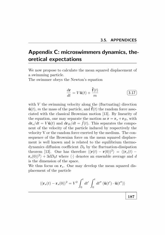
3.5. APPENDICES
Appendix C: microswimmers dynamics, the-
oretical expectations
We now propose to calculate the mean squared displacement ofa swimming particle.The swimmer obeys the Newton’s equation
dr
dt= V u(t) +
f(t)
m
3.17
with V the swimming velocity along the (fluctuating) directionu(t), m the mass of the particle, and f(t) the random force asso-ciated with the classical Brownian motion [13]. By linearity ofthe equation, one may separate the motion as r = rs+ rB , withdrs/dt = V u(t) and drB/dt = f(t). This separates the compo-nent of the velocity of the particle induced by respectively thevelocity V or the random force exerted by the medium. The con-sequence of the Brownian force on the mean squared displace-ment is well known and is related to the equilibrium thermo-dynamics diffusion coefficient D0 by the fluctuation-dissipationtheorem [13]. One has therefore 〈(r(t) − r(0))2〉 = 〈(rs(t) −rs(0))
2〉 + 3dD0t where 〈·〉 denotes an ensemble average and dis the dimension of the space.We thus focus on rs. One may develop the mean squared dis-placement of the particle
〈(rs(t)− rs(0)〉2 = V 2
∫ t
0
dt′∫ t
0
dt′′ 〈u(t′) · u(t′′)〉
187

CHAPTER 3. JANUS MICROSWIMMERS
which can be rewritten
〈(rs(t)− rs(0)〉2 = V 2
∫ t
0
ds (t− s)C(s)
3.18
with C(s) = 〈u(s) · u(0)〉.The next step is to compute this correlation function. The par-ticle undergoes a rotational Brownian motion, and the distribu-tion P (u, t) obeys the rotational diffusion equation:
∂tP (u, t) = Dr ∆θ,φP (u, t)
where ∆θ,φ = L2 is the rotational Laplacian operator (also de-
fined in terms of L, the angular momentum operator).The solution to this equation with initial condition P (u, t =0) = δ(u− u0) takes the form:
G(u, t|u0) =∑
ℓ,m
Yℓ,m(u)Yℓ,m(u0) exp[−ℓ(ℓ+ 1)t/τr]
(τr = 1/Dr), so that the complete solution is
P (u, t) =
∫
du0 P0(u0)×G(u, t|u0)
with P0(u0) the initial distribution.Finally we can deduce the correlation function
C(t) =
∫
du0
∫
du P0(u0)×G(u, t|u0) u · u0
188
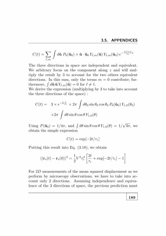
3.5. APPENDICES
C(t) =∑
ℓ,m
∫
du P0(u0)× u · u0 Yℓ,m(u)Yℓ,m(u0) e−
ℓ(ℓ+1)τr
t
The three directions in space are independent and equivalent.We arbitrary focus on the component along z and will mul-tiply the result by 3 to account for the two others equivalentdirections. In this sum, only the terms m = 0 contribute; fur-thermore,
∫
du uYℓ,m(u) = 0 for ℓ 6= 1.We derive the expression (multiplying by 3 to take into accountthe three directions of the space) :
C(t) = 3× e−2 tτr × 2π
∫
dθ0 sin θ0 cos θ0 P0(u0)Y1,0(θ0)
×2π
∫
dθ sin θ cos θ Y1,0(θ)
Using P (u0) = 1/4π, and∫
dθ sin θ cos θ Y1,0(θ) = 1/√3π, we
obtain the simple expression
C(t) = exp[−2t/τr]
Putting this result into Eq. (3.18), we obtain
〈(rs(t)− rs(0)〉2 =1
2V 2τ2r
[
2t
τr+ exp[−2t/τr]− 1
]
For 2D measurements of the mean squared displacement as weperform by microscopy observations, we have to take into ac-count only 2 directions. Assuming independence and equiva-lence of the 3 directions of space, the previous prediction must
189

CHAPTER 3. JANUS MICROSWIMMERS
be multiplied by 23 . Adding the Brownian component of the
mean squared displacement, we obtain the final formula for ameasured mean squared displacement:
〈(rs(t)− rs(0)〉2 = 4D0t+1
3V 2τ2r
[
2t
τr+ exp[−2t/τr]− 1
]
3.19
190

3.5. APPENDICES
Appendix D: sedimentation, experimental
benchmarks
In order to probe the validity of a fluctuation-dissipation rela-tionship with a suspension of active colloids, we measure thedensity profiles of the colloids in a microfluidic chamber. In thissection, we perform experiments at equilibrium in order to cal-ibrate and validate our experimental setup.We want to measure the density profile ρ(z) of a dilute solutionof colloids (Φ ∼ 0.01%) in water, at equilibrium at temperatureT . We use the same commercial colloids (F8823, lot 21681W,Molecular Probes) as used to synthesize the Janus particles. Thesolution is enclosed in a gel microfluidic chamber as described inAppendix B. The system is left at rest during 4 hours to reachthe steady diffusion coefficient.
Counting colloidsAfter this time we perform z stacks by scanning the chamberwith a piezo (see section 3.4). We want to count the number ofcolloids “close to the focus” on each frame and sum the resultsfor a given altitude z. This way we can measure the colloids dis-tribution along the z direction. For now the expression “close tothe focus” is willingly a blurry concept that we must define morequantitatively. The fluorescent intensity profile I(z) of the maxi-mum intensity is measured to determine accurately the distanceof a colloid to the focus plane. We measure experimentally thefluorescent intensity I(z) of an adsorbed colloid on a glass slidewith a water immersion high numerical aperture objective (N.A.
191

CHAPTER 3. JANUS MICROSWIMMERS
10 20 30 40 500
1000
2000
3000
4000
5000
z(!m)
N(z
)
b)
(4 (2 0 2 40
0.2
0.4
0.6
0.8
1
z(!m)
I/I 0
a)
10 20 30 40 500
0.2
0.4
0.6
z(!m)
N/N
0
Figure 3.15: (a) z profile of fluorescence intensity of a colloid (redsymbols). A fluorescent colloid is adsorbed on a glass slide. A piezo scansthe fluorescent intensity of the brightest pixel along z by steps of 200 nm.The fluorescence intensity I(z) is well fitted by a gaussian function (blackdashed line). (b) Equilibrium sedimentation profiles. Steady densityprofiles of colloids measured for sedimentation experiments of latex colloidsat equilibrium in water. The different symbols represent the density pro-files extracted from stacks of images for various thresholds: 0.3Ifoc (⋄),0.5Ifoc () and 0.6Ifoc (). For each case the profile is exponential (dashedline) and the exponential decay does not depend on the threshold criterionb0 = 12.1± 1µm. Inset Normalized density profiles all collapse to thesame exponential curve in good agreement with the theoretical value. Thisbenchmark experiment fully validates the experimental setup.
192

3.5. APPENDICES
1.2). The normalized intensity is depicted in figure 3.15-a. Theintensity is well fitted by a Gaussian. This curve calibrates therelationship between the threshold criterion (in percentage ofthe intensity in the focus plane Ifoc) and δ. Applying a thresh-old criterion we can suppress on each frames the colloids thatare at a distance beyond δ of the focus plane and count thecolloids present in the slice ±δ. Practically, a high thresholdeases the determination of “in focus” colloids but diminishesthe statistics of particles detected on each frame. To get suf-ficient number of particles and good statistical convergence wedefine slices of thickness ±2µm. This implies a threshold cri-terion determined by 0.3Ifoc. Moreover, the determination ofδ also impacts the acquisition time Tacq between frames. Toperform a proper ensemble average, Tacq must be large enoughto enable a colloid to diffuse into or out of the slice. This givesTacq ≥ δ2/2D ∼ 3 s with D the diffusion coefficient of the col-loids (typically 1µm2/s for an active colloid) and supports theacquisition frame rate used of 0.2− 0.3Hz.
Tribute to Jean PerrinFinally, we measure the density profile of latex colloids in water.The results are presented in figure 3.15-b. The distribution ofcolloid is (i) steady, (ii) exponential with (iii) an exponentialdecay over a characteristic length b0 = 12 ± 1µm. This valueis in full agreement with Jean Perrin expectations for equilib-rium. Indeed, for latex colloids (density d=1.055) with radiusR = 0.55±0.02µm at ambient temperature, one expects a sedi-mentation length given by Eq-3.13: b0 = 10.9±1.2µm. This re-sult fully validates our experimental setup. Moreover we checked
193

CHAPTER 3. JANUS MICROSWIMMERS
that varying the threshold criterion only affects the number ofdetected colloids but not the exponential behavior and the de-cay length b0. In the figure 3.15-b, density profiles of colloidsare represented from the same experiments and extracted forvarious threshold criterions: 0.3; 0.5 and 0.6Ifoc. We verify thatfor each case the distribution is exponential with the same expo-nential decay b0 (see Fig. 3.15-inset) and that only ρ0 is affectedwhich finishes to validate our experimental canvass.
194

Quand y en a un, ca va, c’est quand y en a beaucoup
que ca pose probleme1.
B. Hortefeux, Sep. 2009
4Towards collective behaviors
The results depicted in the previous chapter on dilute assem-bly of Janus microswimmers are equilibrium-like and properlydescribed in the framework of a Fluctuation-Dissipation rela-tionship. In this context, they do not demonstrate importantbreakdown of equilibrium physics –certainly related to the di-lute concentration of swimmer– but are a key first step to ad-dress more complex behaviors of active matter. Indeed collectivemotion can be observed at almost every scale in nature, fromthe familiar human crowds, bird flocks and fish schools to mi-croorganisms such bacteria, or cells and until nanometric levelwith the dynamics of actin and tubulin filaments and the syn-chronization of molecular motors. Whereas biologists tend tobuild detailed representations of a particular case, the ubiquityof the phenomenon suggests underlying universal features andthus gives weight to the bottom-up modeling approach favored
1Unfortunately it did not refer to the complexity of large systems.
195

CHAPTER 4. TOWARDS COLLECTIVE BEHAVIORS
by physicist. It is thus natural for a condensed matter physi-cist to regard a coherently moving phase as an orientationallymoving phase. This motivated a huge amount of work to un-derstand this broad class of non-equilibrium dynamical systems.
Aim of this chapter
In this fourth and last chapter, I will present a brief review of the–huge–literature on collective effects, designed for experimental-ists. The theoretical predictions in this field are abounding butscattered which makes the classification of real systems a bitawkward. This impression in magnified by the scarcity of experi-mental results to validate the numerous theoretical models. Theaim is thus to point relevant, and experimentally accessible, ob-servables and signatures related to the “out-of-equilibriumness”of active systems. In this scope, I will report theoretical predic-tions as well as experimental demonstrations of these effects.The main purpose is to open perspectives and offerguidelines for further experimental studies of active sys-tems. As I began exploring collective behavior of active colloidsonly at the end of my PhD, I will report here only very prelim-inary experimental results with dense suspensions of the Janusdiffusio-phoretic microswimmers I have previously studied in thesemi-dilute regime (see chapter 3). Encouraging experimentalhints underline the relevance of this system in the study of col-lective behaviors.
196

Organization of the discussion
In a first part of this section I will describe the theoretical resultson the collective and phase behaviors of flocks, i.e. assemblies ofself-propelled particles (SPP) with velocity v0 without solvent.The situation of SPP flocks without solvent may appear as un-connected to the situation of active Janus suspensions for whichthe solvent and hydrodynamic interactions play a crucial role. Iwill nevertheless review this class of SPP as they are some of themajor “toy-models” in the study of active systems. In this re-spect, they are a pleasant avenue to begin in the complex worldof collective behaviors and see some of the various signatures of“out-of-equilibriumness”: giant number fluctuations, emergenceof 2D long range order ...In a second part, I will describe the physics of swimming mi-croorganisms, i.e. self propelled particles in a fluid medium: thesolvent which imposes momentum conservation. This additionalconservation law leads to different characteristics than describedin the first part and underline the role of hydrodynamic interac-tions. I will report theoretical predictions in these systems andexperimental hints to probe active suspension.In this context, further perspectives and preliminary experimen-tal results on dense suspensions of the Janus diffusio-phoreticmicroswimmers I have previously studied in the semi-dilute regime(see chapter 3) will be discussed.
197

CHAPTER 4. TOWARDS COLLECTIVE BEHAVIORS
4.1 Preamble on active systems
As previously mentioned, active matter is condensed matter ina fundamentally new non-equilibrium regime. To support thisidea we underline specificities of these systems:
1. The energy input takes place directly at the scale of eachactive particle and is thus “homogeneously” distributed inbulk, in clear contrast with out-of-equilibrium systems forwhich the energy is injected by a boundary forcing, e.g.sheared fluids.
2. The direction of the self-propelled motion is set by theparticles themselves (and possible couplings with the sur-rounding world) but no symmetry-breaking is imposed byan external field.
Actually these characteristics can even be used to define activematter. The purpose of the physicist is thus to give a compre-hensible framework for the description of such systems and givea proper scenario to describe how interactions typically at theparticle range can lead to the emergence of long range order.We turn to the description of out-of-equilibrium signatures andphase transitions of assembly of SPP. We will notably under-line the differences arising from the different classes of system:SPP without or with surrounding fluid medium and categoriesof propellers (polar/apolar for flocks and pushers/pullers for ac-tive suspensions). As a first step we will consider a “minimal”model of flocking: the Vicsek’s model [87]. Through this modelof individuals coupled via microscopic interacting rules, it will
198

4.1. PREAMBLE ON ACTIVE SYSTEMS
be easier to build an intuition on the collective behavior thatmay arise from a collection of interacting SPP. Such a “micro-scopic” approach allows to figure out many properties of SPPbut does not allow to understand the large scale, long dynam-ics of a very large, moving flock. Solving the very-many bodyproblem is analytically intractable and moreover a priori unnec-essary to describe the large scales in the system. This problemis analogous to the field of hydrodynamics where the dynamicsof the fluid is properly described by a continuum Navier-Stokesequation rather than the complete dynamics of all the molecularcomponents in the fluid. The “coarse-graining” of observablesdescribes the flock into continuum, smooth fields, e.g numberdensity ρ(r, t) or velocity v(r, t). Spatial and temporal sym-metries of the considered problem and the definition of phe-nomenological parameters that “hide” microscopic details, asbulk viscosity η for hydrodynamics, allows to build a propercontinuum evolution equation of the SPP system. The hydrody-namic approach is a very powerful tool to probe various aspectsof the physics of active matter:
• Noise and phase transitions. For a general SPP suspen-sion one expects noise sources of different kinds: thermalBrownian motion (negligible for particles larger than a fewmicrons)and intrinsic fluctuations in the “motor” of self-propulsion of individuals SPP. The noise competes withthe emergence of long range order and the formation ofcollective behaviors. We will thus discuss “phase transi-tions” and emergence of long ranged order in these sys-tems and the sensitivity of the ordered phases to noise,
199

CHAPTER 4. TOWARDS COLLECTIVE BEHAVIORS
e.g. what is the order of the transition?
• Fluctuations. What are the scaling laws of the fluctuationsin such out of equilibrium systems? Do they agree with thecentral limit theorem as for equilibrium ? We will notablydiscuss number fluctuations in suspensions of SPP.
4.2 SPP flocks
In this section we will begin by addressing models of orderingof active particles in a surrounding medium treated as an inertsubstrate or this equivalent without solvent. Each self-propelledparticle possesses a velocity vector of fixed magnitude v0.
Classification of systems
As a first step we will try to classify SPP in a minimal num-ber of classes influencing the collective dynamics of the flock.Propulsion The mode of propulsion of the SPP belongs to oneof the two following type:
• polar: the particles possess a “head” and a “tail” and thedirection of the propulsion is thus given by an arrow. Thisis of course the case of birds, bacteria ...
• apolar: the particles are moving in a direction but withindifferent tail or head. Such systems can be experimen-tally obtained from symmetric rods in a vibrated con-tainer: the velocity is given by the long axis of the cylinderbut the direction is random.
200

4.2. SPP FLOCKS
A B t t’>t t t’>t
Figure 4.1: Classifications of interactions between self-propelledparticles. We consider only polar SPP, blacks arrows represent velocityvectors. A. Ferromagnetic interactions: aligns the velocity vectorof interacting SPP in direction and sense, for any given initial conditionsbefore interaction.B. Nematic interactions: aligns the velocity vector of interacting SPP.Nevertheless final velocities can be parallel or antiparallel depending onthe initial angle between the polar SPP. A simple picture is that nematicinteraction tends to align vectors with minimal geometric change in thesystem.
201

CHAPTER 4. TOWARDS COLLECTIVE BEHAVIORS
InteractionsThe emergence of collective behaviors relies on the presence ofinteractions between the particles. Even short range interac-tions as excluding volume can be sufficient. We classify interac-tions in the same spirit as the propulsion mode of the SPP, on“geometrical” bases.
• Ferromagnetic interactions. Considering two polarSPP interacting, the interaction aligns the directions andsenses of the velocity vectors (see Fig.4.1-A). Of course,ferromagnetic interactions do not make sense for apolarSPP!
• Nematic interactions. Considering two polar SPP in-teracting, the interaction aligns the directions and arrowsof the velocity vectors if the initial angle between them isbelow π/2 and aligns in direction but with opposite senseotherwise (see Fig.4.1-B).
4.2.1 Polar SPP with ferromagnetic interac-tions: Vicsek’s model and further
Ingredients of the model
We begin by the description of a microscopic, discrete model offlocking: the Vicsek model [87]. The purpose is to define theminimal ingredients to obtain through numerical simulationscollective behaviors of SPP as birds.The model incorporates the following generic features
202
4.2. SPP FLOCKS
1. A large number of polar points SPP.
2. Interactions are ferromagnetic. Particles move over timeattempting to move in the same direction as their neigh-bors.
3. Interactions are purely short-ranged: each SPP will tendto follow its neighbors within some finite distance1 R0,independent of the size of the flock.
4. The model has complete rotational symmetry.
5. The SPP mechanism of “following” is noisy. The only con-sidered noise is on the direction it actually moves addingto the averaged direction of motion a stochastic, short-ranged spatio-temporally correlated noise –while the ve-locity magnitude is kept constant.
6. The considered model is purely 2D.
Results and discussion
An equilibrium-like XY ferromagnetFirst, as first noted by Vicsek himself, this model is exactly the
1This may appear as a reasonable assumption for bird flocks but is actu-ally wrong. The constraint on the interactions is not geometric (interactionif the distance between birds is below R0) but topological in nature (thereare interactions between the n neighboring birds even if they are distantfrom more than R0) as experimentally unveiled by the Starflag team [100]The topological interaction moreover grants significantly higher cohesionon the aggregation of the flock compared with the metric, geometric one.
203

CHAPTER 4. TOWARDS COLLECTIVE BEHAVIORS
dynamical model for a 2D equilibrium ferromagnet except forthe motion. If we thus interpret the velocity vectors of theSPP vi as spins carried by each “bird” and update the spins ac-cording to the given rule for the interaction but do not actuallymove the birds, the model is a an equilibrium 2D ferromagnetwhich will relax to a Boltzmann distribution for an equilibriumHeisenberg model (with spins on a random set of points ratherthat on a lattice as usually stated). The Vicsek’s model thusshares many analogies with the XY magnet models: it presents a“well defined” phase transition from a disordered phase to a co-herent flock with decreased noise or increased particles density.The nature of the order-disorder transition with noise strengthis under debate. Originally pointed as a second order transitionby Vicsek [87], the transition was revealed to be discontinuousby Gregoire et al. by using much larger systems [143]. The crit-ical behavior advocated by Vicsek was then attributed to strongfinite size effects.
An out-of-equilibrium signature: emergence of a long range or-derA striking difference with ferromagnetic analogy arises fromVicsek’s simulations: at large density and low –but non zero–noise, the motion tends to become ordered from disordered ona macroscopic scale and all the particles tend to move in thesame spontaneously selected direction (see Fig-4.2). The flock-ing model thus shows that a true long range order, i.e. acoherently, moving ferromagnetic flock with a nonzero averagevelocity 〈v〉 = 1
N
∑
i vi, is possible at “nonzero temperature”,i.e. nonzero noise. This result is in clear disagreement with
204

4.2. SPP FLOCKS
the “Mermin-Wagner” theorem of equilibrium statistical me-chanics. This theorem states that (i) in dimensions d ≤ 2, (ii)at non zero temperature with (iii) short-ranged interactions,it is impossible to spontaneously break a continuous symme-try. In the context of the XY spin model, it means that isimpossible to develop spontaneously a true long-range orderedstate with nonzero magnetization from a disordered state, withzero magnetization. But the ordered state with 〈v〉 6= 0 breaksthe continuous symmetry of the disordered state, namely ro-tation invariance! The reason the Mermin-Wagner theoremdoes not apply to flocks is of course that they are not systemsin thermal equilibrium due to the intrinsically non-equilibriumself-propulsion of the particles! The kinetic disordered-orderedphase transition is related to the fact that the particles aredriven with a constant absolute velocity and thus unlike stan-dard equilibrium physical systems, with no conservation of thetotal momentum in the system. Finally, the spontaneous emer-gence of a moving, ordered phase thus appears as a strong sig-nature of the “out-of-equilibriumness” of the SPP in Vicsek’smodel.
Further properties of ferromagnetic flocks
The “microscopic” Vicsek model is of great interest in order tofigure out the physics at work in the emergence of long rangedorder in assemblies of SPPs. As we briefly mentioned in theintroduction, such a detailed description is not adapted to thedescription of the large-scales, long-time dynamics of a large as-sembly of particles which requires a hydrodynamics formulation.
205

CHAPTER 4. TOWARDS COLLECTIVE BEHAVIORS
Figure 4.2: Disordered-ordered phase transition in a system ofSPP following Vicsek’s model. The actual velocity is depicted by ablack arrow. (a) Initial conditions. (b) For small densities and noise, theparticles form groups moving coherently in random directions–disorderedphase. (c) At higher density and noise, the particles move randomly butwith some correlation–disordered phase. (d) For higher density and smallernonzero noise,long-ranged order emerges and the phase is ordered. Reprintfrom [87].
206

4.2. SPP FLOCKS
We will not describe the way continuum equations of the hydro-dynamic model are written-down and derived. Basically, thegeneral principle is that the non-equilibrium conditions obligeto consider all terms in the equations that are not explicitlyforbidden by symmetry or conservation laws. The interestedreader can report to [144–146] for these aspects. Now, we onlyreport additional –but non exhaustive– insights on the physicsof ferromagnetic flocks given by the hydrodynamics formulationthat appear as signatures of the non-equilibrium nature of thesystem and that could be tested experimentally:
• Long range order in 2D. Taking into account the nonlinearities of the hydrodynamics equation, it is shown that2D long-range order is possible in a ferromagnetic flock asobtained from the Vicsek model
• Anomalous number fluctuations. The density fieldpresents anomalous strong fluctuations2 in the orderedphase. For regions with N particles on average, the rootmean square of the fluctuations ∆N = 〈(N(t) − N)2〉 1
2
scales a Nγ with γ = 0.8 > 0.5 [147].
• Anomalous transverse diffusion in the ferromag-netic phase. Simulations unveiled an anomalous superdif-fusion of individual particles in the direction perpendicularto the flock’s moving direction. The dispersion of a 2D en-semble of “boids” is given by w2(t) = 〈[yi(t)−yi(0)]〉 ∝ t
43
2As a quick reminder, the root mean square of the fluctuations of an
observable ∆O ∝ O12 in a equilibrium system, given the central limit the-
orem.
207

CHAPTER 4. TOWARDS COLLECTIVE BEHAVIORS
[145]. Note that the diffusion remains anomalous in 3Dbut the scaling law differs: w2(t)〉 ∝ t1.7 [147].
4.2.2 Polar SPP with nematic interactions
Theoretical predictions
We now turn to large collections of polar SPP with nematicinteractions restricted to a two dimension space. This classof SPPs can be practically obtained from anisotropic vibratedrods, thus polar [148,149] interacting through volume exclusion,which is nematic (as figured out by Fig.4.1-B) . This problemwas addressed in a mixed Vicsek model by Chate et al. [147].Once again, we report only major and experimentally accessiblesignatures of the non-equilibrium properties that are much moreextensively discussed in [131,150].
• Nematic ordered phase. Unlike polar SPP with ferro-magnetic interaction, no polar ordered phase is observedin this system. Only nematic order arises in spite of thepolar nature of the particles, but it is long-ranged.
• Phase transitions and anomalous fluctuations. Thissystem exhibits a much more complex phase transition be-havior that in the ferromagnetic case: ordered and disor-dered regimes, each sub-divided in two phases leading to atotal of four phases [150] (see Fig-4.3). Given the particledensity, the nematic orientational order is destroyed withincreasing noise.
208

4.2. SPP FLOCKS
– Phase I: at lowest noise η, presence of a long range ne-matic order. Two subpopulations of particles migratein opposite directions constantly exchanging parti-cles (see Fig-4.3-a). Anomalous number fluctuationsappear in this phase: ∆N ∝ 〈N〉0.8, as for the ferro-magnetic polar order.
– Phase II: at steady state, presence of the low-densitydisordered region (see Fig-4.3-b,c). The emergence ofthe density inhomogeneities processes as nucleationand phase separation. The dense regions presentsnematic order as for phase I and similar anomalousfluctuations.
– Phase III: segregated system with presence of densebands (see Fig-4.3-d). The bands are unstable andchaotically bend, break and reform. Phase III is adisordered phase with normal equilibrium-like fluctu-ations but huge temporal and spatial correlations.
– Phase IV: highest noise, ordinary, spatially homo-geneous disordered phase with very short time andspace correlations.
• Isotropic-nematic transition. Hydrodynamic descrip-tion of a system of polar SPP with nematic shows a lower-ing of the density parameter ρSPP of the nematic-isotropic
transition: ρSPP = ρE/(1 +v20
5kBT ), where v0 is the SPPvelocity and ρE the equilibrium Onsager transition den-sity [131]
209

CHAPTER 4. TOWARDS COLLECTIVE BEHAVIORS
• Boundary conditions sensibility. We want to stress avery important role played by boundary conditions in thephysics of SPPs. For equilibrium system, the boundarylayer typically develops in a scale δ ∼ ℓ given by the size ℓof the particle. With active systems, a finite polarizationat the boundary decays as δ ∼ v0τ , with τ the persistencetime in the system. Given L the size of the system, ifL ∼ v0τ , the correlations develop on the same scale as thesize of the system. This underlines the possible prime roleof boundary conditions in such systems as well as possibleexperimental arctefacts.
• Clustering transition. A clustering transition exists forparticles with only excluded-volume interaction providedactive motion and anisotropic particles (rods). This tran-sition does not exist for isotropic particles (squares) orBrownian equilibrium diffusion [151].
Figure 4.3: Phases in a system of polar SPPs with nematic in-teractions for increasing noise from (a) to (e). Arrows indicate thepolar orientation of the particles. See text for a description of the phaseproperties. Reprint from [150]
210

4.2. SPP FLOCKS
Experimental realizations
Experiments with large collection polar self-propelled particleswere performed by Kudrolli et al.. Vibrated anisotropic rods be-have as polar particles [149] and interact via volume-excludednematic interactions. For sufficient driving accelerations, theyobserve dense clustering of self-propelled rods at the boundary.This phenomenon is absent for self-propelled rods which seemsin agreement with the theoretical predictions by [151]. The clus-tering at the wall underlines the predominant role of boundaryconditions in these systems. Anomalous number fluctuationsare reported: ∆N ∝ 〈N〉 7
12 , but with an exponent differentfrom Ginelli et al. predictions [150]. Finally, no global polarorder is observed in the system but coherent structures appearand the velocity field reveals numbers of streams and swirls withstrong random fluctuations.Recently, Deseigne et al. performed experiments with asymmet-ric, polar, vibrated disks. Interactions are given by hard corerepulsion [139]. They observe anomalous number fluctuations∆N ∝ 〈N〉0.72 in good agreement with 0.8 exponent theoret-ically predicted3. Finally they report polar collective motionwith long-range order –developed on the scale of the system–. The emergence of a polar order is not expected theoreticallyfor polar SPP with nematic alignment (but predicted for polarSPP with ferromagnetic interactions). Actually they observenematic collisions with systematic ferromagnetic bias. The con-
3Note that we define ∆N as the root mean square of the fluctuationsin the whole chapter while Deseigne et al. used the same notation for thevariance of the particles number in [139] thus the square of our notation.
211

CHAPTER 4. TOWARDS COLLECTIVE BEHAVIORS
sequences of this additional ingredient has not been consideredup to now theoretically and make the classification of the systemawkward. This result questions the nature of the of the interac-tions in this system that would a priori be pointed as nematicbut nonetheless presents experimental ferromagnetic bias.
We end this section on SPP without solvent with the case ofapolar SPP with nematic interactions.
4.2.3 Active nematics
By symmetry, the mean macroscopic velocity of an active ne-matic flock is zero. One could then imagine that the systempresents no distinctive nonequilibrium properties since a phasethat is not drifting does not have an order parameter thatbreaks time-reversal symmetry [146]. This expectation is ac-tually wrong and dynamical processes allowed by the symmetryof the system introduce remarkable statistical behaviors of ac-tive nematics.
Giant number fluctuations
The main prediction on the non-equilibrium signature of ac-tive nematics is the presence of giant number fluctuations, i.e.∆N ∝ 〈N〉 in strong contrast with equilibrium situations wherecentral limit theorem applies and with an anomalous exponentbigger than with other class of SPP systems. Such fluctuationsare named giant as they make the density an ill-defined quantityeven in the limit of a large system. A physical understanding ofthe origin on the giant number fluctuations of the system can
212

4.2. SPP FLOCKS
be pictured as follows [152]. We consider a 2D system of apolarnematic SPP, with the angle θ as the only parameter to defineflock distortions from perfectly aligned state. As presented onFig.4.4-a, any asymmetry in the flock, splay or bend, conferslocal polarity and hence local flock motion. The current of par-ticle J is thus proportional to the angular gradients: ∂xθ, ∂zθ.At steady state, this active flux is balanced by the diffusive cur-rent JD ∝ ∇ρ, ρ density of the flock which makes fluctuationsof ρ and θ of same order.By symmetry, angular θ fluctuations have variance of order 1/q2
at wavenumber q and thereafter, number density fluctuationsare of 1/q2. Integrating over the wavenumber in a 2D space,one finally obtains the number fluctuations.
∆N ∝ 〈N〉 12+
1d ∼ 〈N〉 with d = 2, the space dimension
The giant number fluctuations thus appear as a consequence ofthe coupled dynamics of density and orientation related to thenematic order in the system. So forth no giant fluctuations areexpected in the isotropic phase.
Experiments
Narayan et al. realized experimental active nematics with avery dense collection (surface fraction Φ ∼ 50 − 66%) of agi-tated monolayer of rods on a solid substrate. They measuredgiant number fluctuations ∆N ∝ 〈N〉 in a system presentingmacroscopic swirls [153] (see Fig.4.4-b) . No giant fluctuationsare reported in the isotropic phase. The fluctuations are alsoextremely long-lived as they report logarithmic relaxation of
213

CHAPTER 4. TOWARDS COLLECTIVE BEHAVIORS
the temporal autocorrelation function of the density fluctua-tions. Both these experimental results agree with theoreticalpredictions on active nematics [153,154]. I end up with the brief
a) b)
Figure 4.4: Giant number fluctuations in active nematic. (a) Bendor Splay in an apolar nematic confers local polarity and hence local motion.Reprint from [152]. (b) Nematic order with giant density fluctuations in aassembly of active nematic particles. Reprint from [153].
overview of the complex dynamics of self-propelled particles with-out solvent or, this is equivalent, a passive frictionnal mediumwhich only role is to keep the particles at constant velocity. Inow add a fluid solvent and consider the collective behaviors ofsuspended swimmers. The motion of the active particles in themedium is force free and for this class of SPP and additionalconservation law is to be accounted: momentum conservation.This arises hydrodynamics interactions which present importantmodifications in the dynamics.We will restrict ourselves in our presentation to the case of thelow Reynolds regime e.g. with microorganisms and in Newto-nian fluids.
214

4.3. LOW REYNOLDS NUMBER ACTIVE SUSPENSIONS
4.3 Low Reynolds number active suspen-
sions
In this section we therefore survey such suspensions, orderedor disordered, of active particles in a fluid medium and showhow the inclusion of momentum-conserving hydrodynamic flowinto the analysis of active particle systems introduces impor-tant qualitative departures from the behavior presented in thepreceding section. The long-range nature of the hydrodynamicinteractions among the active particles leads to large-scale nonequilibrium phenomena reported in colonies of bacteria of col-lections of living cells.
4.3.1 Pushers and Pullers
Low Reynolds microorganisms propel through a variety of pe-riodic, non-reciprocal strokes (as described in section-3.1) thatinvolve complex dynamics of beating parts e.g. flagella or cilia.Understanding the collective behaviors of dense suspensions ofthese systems, given the details of the swimming dynamics ofindividuals, would appear as a complete nightmare. Here weare interested in the collective behavior of many swimmers onlong time and large length scale which make the details of themechanism of self propulsion cumbersome.
Given Newton’s third law, the active particles and the fluid ex-ert equal and opposite forces on each other. It imposes that the
215

CHAPTER 4. TOWARDS COLLECTIVE BEHAVIORS
force density associated with each swimmer must integrate tozero, i.e no monopole moment is allowed. In a far field approx-imation, the minimal model of a stroke-averaged active particlein a fluid is therefore a static force dipole4 of strength f , positiveor negative, depending on the force exerted on the surroundingfluid:
• Pullers. Contractile swimmers with f < 0 pull fluid alongtheir axis and push fluid out along an axis normal to theirmidpoint (see Fig.4.5-A for the fluid flow pattern). Theyare propelled by flagella at the head of the organism, hence“pullers”. The algae Chlamydomonas belong to this class.
• Pushers. Tensile swimmers with f > 0 push fluid alongtheir axis and pull fluid at their midpoint (see Fig.4.5-B forthe fluid flow pattern). They are propelled from the rear,hence “pushers”. Most bacteria, such as E. Coli belong tothis class.
Let us precise that using the classification of SPP given in theprevious section swimmers are polar particles.
The theoretical study of active suspensions is done by construct-ing the coupled dynamical equations for the swimmer concentra-tions and orientations and a generalized Navier-Stokes equationfor the velocity field u of the suspension. Self-propulsion entersvia the force density f in Navier-Stokes equation. The formu-lation of the hydrodynamic equations and their study goes far
4More complex models may encounter higher order multipoles.
216

4.3. LOW REYNOLDS NUMBER ACTIVE SUSPENSIONS
beyond the aim of this chapter but are thoroughly developedin [86, 137, 146, 152]. Only most striking consequences on thedynamics or anomalous observables and experimental illustra-tions will be discussed.
4.3.2 Breaking the second principle
Thanks to the permanent energy input by the active swimmers,the system is intrinsically out-of-equilibrium and thus has noreason to be ruled by equilibrium principles as the second prin-ciple. Recently, Di Leonardo et al. gave numerical evidences ofmonothermal micromotor in a bacterial bath [101]. The chaoticmotion of the active particles is rectified by asymmetric environ-ment, e.g. ratchets to give net propulsion. This result is in clearcontrast with equilibrium baths for which the detailed balancecan not be broken. This scenario was validated experimentallyby [102,103]
4.3.3 Instability of orientation-ordered activesuspensions
Instability of orientation-ordered active suspensions
Uniform ordered active suspensions are absolutely unstable atlong wavelengths because of the growth of orientational fluctu-ations [86,152]. An orientational order is under permanent andunstable uniaxial compression (pullers) or tension (pushers). Weshow the basic mechanism at work for suspensions of pullers(see Fig.4.5-A’) or pushers (see Fig.4.5-B’). Let us consider a
217

CHAPTER 4. TOWARDS COLLECTIVE BEHAVIORS
A
B
A’
B’
Figure 4.5: (A-B) Dipolar flow pattern induced by the active forceexerted on the surrounding fluid by a puller (A) or a pusher (B).The arrows represent the direction of the flow, fluid flow velocity denoted bythe color. White arrow gives the direction of propulsion. Reprint from [137].(A’-B’) Instability of a polar-ordered suspension of pullers (A’)or pushers (B’). Let us assume a perfectly ordered, unbounded, parallelcollection of pullers (A’), respectively pushers (B’), (swimmers representedas full colored symbols), i.e. a polar-ordered state. The double black arrowshows that any fluctuation of orientation of a swimmer (open red symbol) isamplified by the flow pattern (grey arrows) of the neighboring pullers (A’)or pushers (B’) (full blue symbols). Polar state of pullers, respectively, isan unstable state of uniaxial tension, respectively compression.
218

4.3. LOW REYNOLDS NUMBER ACTIVE SUSPENSIONS
perfectly ordered, unbounded parallel collection of pullers (re-spectively pushers) swimmers. The self generated flows cancelin a delicate balance and the polar-state is at equilibrium. Thenature of the equilibrium –stable or unstable– is given by the ro-bustness to fluctuations. We suppose an orientation fluctuationof one puller (respectively pusher) in the polar state. The fluctu-ation is amplified by the flow pattern induced by the neighboringpullers (respectively pushers) and destabilizes the orientationalorder into an isotropic state (see Fig.4.6-I).This scenario is in full agreement with the theoretical expressionderived by [137] of the torque exerted by a puller (respectivelypusher): a puller tends to misalign other swimmers located inthe orthogonal direction of its axis, and a pusher tends to mis-align swimmers along its axis. This pictorial argument can bedetailed by a stability analysis of the hydrodynamics equationsof the active suspensions [86]. In the Stokesian limit, Simha etal reports a growth of the orientational instability for wavenum-bers q such as Re ≪ qa ≪ Φ
12 , where Re is the Reynolds number
on the scale a of the particle, and Φ is the suspension volumefraction. This prediction differs from recent numerical simu-lations by Saintillan et al. who find that suspensions are al-ways unstable at finite wavelength [155]. Finally, Baskaran etal. underlined the role of the long ranged (∼ 1/r2) nature ofthe hydrodynamic interactions in this instability [137].
Isotropic suspensions: local nematic-order and mixing
In agreement with previous theoretical predictions, numericalsimulations by Saintillan et al. exhibit ordered suspensions of
219

CHAPTER 4. TOWARDS COLLECTIVE BEHAVIORS
e)
a) b)
c) d)
a) b)
c) d)
I) II)
III)
Figure 4.6: I) Destabilization of an orientational order polar stateof pushers into an isotropic state. The isotropic state presents localorder with swirls and vortices . (a)-(d) increasing time in numerical simu-lations: (a) initial polar suspension, (d) final isotropic suspension. Typicalflow field of the isotropic suspension is presented on figure e). Reprintfrom [156]. II) Fluid mixing by an active suspension of pushers.The figure shows the configuration of a passive scalar field in the suspension(a)-(d) increasing time in numerical simulations: (a) initial polar suspen-sion, (d) final isotropic suspension. Reprint from [155].III) Zero reynolds number turbulence in a drop of Bacillus subtilisbacteria (pushers). Reprint from [157].
220
4.3. LOW REYNOLDS NUMBER ACTIVE SUSPENSIONS
swimming rod-like particles unstable to long wavelength [156].Nevertheless they unveil a local nematic ordering at short lengthscale as a result of hydrodynamic interactions. Very rapidly theorientational order destabilizes into a globally isotropic statecharacterized by large-scale vortices and swirls (see Fig.4.6-I.e)with large particles concentration fluctuations. Local orienta-tional order, as well as formation of transient aggregates of par-ticles has been also reported for spherical swimmers5 in [88]with a slow decay of the radial distribution function go(r) ofthe system. These patterns are dynamically unstable and con-stantly break up and merge in time. This suggests importantmodifications on the transport properties, e.g. mixing, in activesuspensions. Saintillan et al. report that efficient convectivemixing takes place in suspensions of pushers (see 4.6-II) but notin suspensions of pullers [155]. The mixing originates in the con-stant breakup and merging of concentrated regions of swimmers.The viscous fluid in which locomotive energy of individuals mi-croswimmers is transferred also carries interactions that drivespatiotemporal coherence. Hydrodynamic couplings has signif-icant impact on the dynamics of the swimming particles. Thevelocity distribution P (v) presents large discrepancies with theequilibrium gaussian distribution. It is algebric P (v) ∼ 1/v atsmall velocities while the asymptotic decay is consistent witha gaussian [88]. Moreover, Saintillan et al. report that pullersswim more slowly than in the isolated case and pushers are
5Local orientational order is also reported for symmetric spherical swim-mers by [88] but without formation of –even transient– aggregate. Nonethe-less, we present this result only as a side remark as symmetric swimmersare rarely encountered in experimental realizations of swimmers.
221

CHAPTER 4. TOWARDS COLLECTIVE BEHAVIORS
faster. This effect exists in a wide range of concentrations –from moderate to high– of swimmers and leads to modificationsof the swimming velocity of an individual up to 15− 30% [156].Furthermore they report a strong dependence with particles vol-ume fraction of the characteristic time scale τr for relaxation ofthe particle orientation. Because the particles interact and ef-fectively travel through a chaotic flow –which depends on theswimmer volume fraction in the suspension– their orientationsactually decorrelate in time.
Experimental observations
Many experimental evidences of “out-of-equilibriumness” of ac-tive suspensions were recently reported, but up to now, onlywith biological microswimmers e.g. bacteria or algae. Recentexperiments have demonstrated the existence of collective effectsfor sufficiently concentrated suspensions [157]. The correlationlength of the collective motion can exceed the size of the individ-ual cells by more than an order of magnitude and the collectiveflow speeds (typically 50-100µm/s) largely exceed the speed ofindividuals (typically 15-20µm/s). Moreover these cooperativeeffects are demonstrated as strongly related to the concentrationof swimmers. No collective effect is observed in dilute suspen-sions in which the correlation length is limited to the size of abacterium, i.e. an equilibrium-like behavior and Sokolov et al.demonstrated a smooth and monotonically increase of the corre-lation length through the transition from individual to collectivebehavior [94].
Experiments by Wu et al. showed the presence of small
222

4.3. LOW REYNOLDS NUMBER ACTIVE SUSPENSIONS
swirls and jets of cooperative swimming in thin films of con-centrated suspensions of bacteria E. Coli –pushers–. This hadimportant impact on the transport properties of the suspensionwith greatly enhanced diffusion6 and even superdiffusion of pas-sive tracers [97]. Exceptional transport of passive species in sus-pensions of pullers, the algae Chlamydomonas, was also recentlyreported with non-gaussian probability distribution functions ofthe tracers displacements by [93].
4.3.4 Rheology of active suspensions
As it propels itself, a swimming particle exerts a net force dipoleon the surrounding fluid as a balance between the propulsiveforce exerted by the particle and the viscous drag on its body.The dipole induces a disturbance flow around the particle whichresults in hydrodynamics interactions, responsible for the com-plex dynamics we described above. In addition, we also expectthat the injection of energy in the system by the active particlesmodifies the effective rheology of the suspension. Large theoret-ical efforts have been recently devoted to study these systems,and provided strong support to the idea that a medium suffusedwith active processes should be thought of as a distinct type ofmaterial. It was notably showed consequences on the viscosity,so called effective viscosity, of the swimming activity. A basicpicture of the connection between bulk viscosity and swimmersactivity can be given as follow. We consider an isotropic sus-
6The idea of a “bacterial bath” akin to the molecular bath responsi-ble for brownian motion arises from the enhanced diffusion of tracers insuspensions of bacteria
223

CHAPTER 4. TOWARDS COLLECTIVE BEHAVIORS
a) b)
Figure 4.7: Impact on the viscosity of the propulsion mode of rod-like swimmers in a isotropic phase of an active suspension. Swimmersalign under shear (black arrow) a) Contractile pullers particles. The forcedipole (red arrow) opposes to the imposed flow, thus leading to an increaseof the effective viscosity of the suspension. b) Tensile pushers particles.The force dipole (red arrow) enhances the imposed flow, thus leading to andecrease of the effective viscosity of the suspension.
pension of rod-like pullers (respectively pushers). A shear flowis imposed to the system and produces alignment of the swim-mers. The permanent force dipole exerted by the contractilepullers (respectively tensile pushers) pulls back and resists to(respectively pushes out and enhances) the flow that orientedthem, see Fig.4.7-a (respectively see Fig.4.7-b). This results ina change in the stress/rate ratio w.r.t. the same equilibrium sus-pension with passive particles, i.e. higher viscosity for pullersand lower viscosity for pushers. This sketch was first given, andsupported by a coarse-grained hydrodynamic approach, by Hat-walne et al [158] to show the macroscopic impact on the viscosityof the swimming activity. These predictions are in agreementwith a kinetic model of active rods by Saintillan [159]. Never-theless the scenario of Fig.4.7 relies on the stress alignment of
224

4.3. LOW REYNOLDS NUMBER ACTIVE SUSPENSIONS
the swimmers, i.e. form anisotropy. Haines et al. showed thatswimming results in a decrease of viscosity only if the orientationdistribution of swimmers is anisotropic, e.g. under gravitationalfield [160] and Ishikawa et al. demonstrated viscosity effects insuspensions of active ”squirmers” in gravity field [161]. Thereduction of effective viscosity intuitively results in the energyinjection by the swimmers thus counteracting the energy lossdue to viscous dissipation [160]. Saintillan formally identifiedthe active power input generated by swimming particles as theorigin for the decrease in viscosity predicted in pusher suspen-sions [159]. He notably demonstrated that predicted negativeviscosity did not violate the positive rate of viscous dissipation,i.e. the second principle of thermodynamics, as it then includeda contribution which is not of dissipative origin. Furthermorewhile positive viscosity results in preferential damping of highwavenumbers, low wave numbers are destabilized by negativeviscosity, thus saturating at large-scale coherent structures inthe absence of any external forcing. This leads to the forma-tion of swirls, whorls or other complex, local structures in densesuspension of microswimmers and reported in the previous sec-tion. Note that theses models are a priori valid for dilute orsemi-dilute suspensions in contrast to the emergence of localswirls that requires dense suspensions of active particles cou-pled by hydrodynamic interactions. For rheological properties,the cooperative alignment of swimmers arises from the shear (orexternal field) but not via hydrodynamic couplings and effectsof activity on viscosity are thus predicted even at concentrationfor which hydrodynamic interaction may be neglected. Non-linear visco-elasticy properties are also expected [158]. Finally
225

CHAPTER 4. TOWARDS COLLECTIVE BEHAVIORS
large fluctuations driven by activity and related to the effectivetemperature of the active system are also reported [158]
Viscosity measurements
Dense suspensions of active swimmersExperimental viscosity measurements has recently been testedon active suspensions of microorganisms. Sokolov et al. de-termined the shear viscosity in concentrated suspensions (vol-ume fraction Φ ∼ 10%) of swimming bacteria Bacillus subtilis –pushers– in a thin liquid film [162]. They monitored the viscoustorque on a rotating particle as well as the decay of a vortex inthe film. They measured a decrease of the effective viscosity byup to a factor of 7 compared to the viscosity of the same liquidwithout bacteria or with nonmotile bacteria. Furthermore, theviscosity depends on the concentration and swimming speed ofthe bacteria, which underlines the crucial role of the microor-ganism activity in the mechanism.Using swimming algae Chlamydomonas Reinhardtii in a conven-tional rheometer, Rafai et al. measured that effective viscosityof concentrated (volume fraction Φ ∼ 20 − 30%) suspensions,i.e. with live –pullers– algae, was far greater than for the sameliquid containing the same concentration of dead algae [99].These experimental results are in qualitative agreement withabove expectations and the basic scenario given on Fig.4.7-a,b):pullers increase the shear viscosity compared to the same pas-sive suspension, while pushers reduce the viscosity. Quantitativecomparisons between models and experiments is still to be per-formed.
226

4.4. PROBING JANUS MICROSWIMMERS
SUSPENSIONS
Dilute/semi-dilute suspensions of active swimmersFinally, Chen et al. probed non equilibrium properties of a di-lute active bacterial bath of E. Coli. In dilute suspensions, withvolume fraction Φ ∼ 10−3%, they measure no departure in therheological response w.r.t. to the equilibrium situation, but sig-nificant enhancement of the fluctuations of the medium thusresulting in a strong violation of the Fluctuation-Dissipationtheorem [163]. They also report anomalous 1/
√
(ω) scalingin the active stress fluctuation spectrum measurements. Thisarises essentially from the concentration fluctuations in the ac-tive stress, but their results underline the importance of the mi-croscopic swimming behavior details in the systems, departuresfrom equilibrium thus proceeding via non-universal mechanisms.
4.4 Probing Janus microswimmers suspen-
sions
We have described many signatures of “out-of-equilibriumness”in suspensions of active self-propelled particles in a fluid medium.Theoretical predictions are numerous in the regime of dense sus-pensions: local nematic ordering with the emergence of complexpatterns of transient swirls and whorls, namely “zero Reynoldsturbulence”, distinctive transport properties, notably efficientmixing only for suspensions of pushers ... Moreover, activityimpacts rheological properties notably increase/decrease of theshear viscosity even in dilute/semi dilute solutions. Many ex-
227

CHAPTER 4. TOWARDS COLLECTIVE BEHAVIORS
perimental validations of some signatures were recently providedwith suspensions but only with active biological microorganismsand requires additional insights with large collections of artificialmicroswimmers. The Janus particles I developed during part ofmy phD thus proposes a relevant avenue in this context. Syn-thesizing the theoretical predictions on active suspensions withthe specificities of the Janus microswimmers, the aim of thissection is to suggest leads to probe out-of-equilibriumsignatures of a suspension of Janus. Furthermore, a fewvery preliminary results will be given as hints of collective effectsin this section
4.4.1 Bulk rheology measurements
One of the most natural way of probe collective effects in activecolloidal suspensions is to perform bulk rheology measurementsin the same spirit as experiments by Rafai et al. or Sokolov etal.. As underlined by [162], the shear viscosity depends on thetotal active energy injection in the medium, i.e. concentrationand velocity of the swimmers. Given the typical velocity of bio-logical microorganisms –typically 20−50µm/s– and the diffusio-phoretic velocity of the Janus microswimmers, V ∼ 1− 3µm/s,it will certainly be necessary to compensate the relatively slowvelocity with higher concentrations, or certainly not lower. Thisunderlines one of the mean experimental difficulty of bulk rhe-ological measurements with artificial swimmers. It will requireto achieve sufficiently highly concentrated suspensions with vol-ume fraction of Janus of order Φ ∼ 10 − 50%. The synthesisof such collections of artificial swimmers as well as the obten-
228

4.4. PROBING JANUS MICROSWIMMERS
SUSPENSIONS
tion of so concentrated suspensions is an experimental challengethat we have not addressed up to now. This track is fully to beexplored!
4.4.2 Passive tracers dynamics in an active bathof Janus microswimmers
Nonetheless Chen et al. demonstrated with passive tracers in abacterial bath that strong departures from equilibrium can arisefrom the energy input even in semi-dilute suspensions of activeparticles Φ ∼ 10−3. I developed in chapter 3 experimental tech-niques to work with Janus suspensions of volume fraction upto Φ ∼ 10−1. In this regime I demonstrated that a suspen-sion of active Janus microswimmers can be well described by afluctuation-dissipation relationship and is equilibrium-like. Nev-ertheless the impact on passive tracers of the activity remainsunexplored in our system. Along this line, it appears interest-ing to study the behavior of passive tracers in an active bath ofJanus microswimmers (with volume fraction Φ ∼ 0.01%). Thiscan be done by measuring the force response of a passive tracerwith optical tweezers which will be interesting to do in the fu-ture or studying its dynamics by optical microscopy.I now present preliminary results for the study of the dynamicsof passive tracers in an active bath of Janus microswimmers.
Experiment
We use, as for the the sedimentation experiments (see section 3.4)a hydrogel microfluidic chamber with Janus particles. In order
229

CHAPTER 4. TOWARDS COLLECTIVE BEHAVIORS
to locally increase the density and magnify the out-of-equilibriumeffets, we use twice heavier Janus particles than in the sedimen-tation experiments. This is done by increasing the platinumcoating to 5 nm –instead of 2 nm– on identical latex particlesbut non fluorescent. A solution containing these Janus particles(ΦJ ∼ 10−2% and dilute passive tracers (φT ∼ 10−4%, fluo-rescent latex particles with diameter 1.1µm) is enclosed in themicrofluidic chamber as previously described. Furthermore, asolution containing only dilute passive tracers (φT ∼ 10−2%,fluorescent latex particles with diameter 1.1µm) is enclosed ina neighboring microfluidic chamber as an equilibrium reference.Hydrogen peroxyde solution at concentration C0 is continuouslycirculated in the lateral channels, ensuring a constant renewalof the fuel and removal of chemical waste (see Fig.4.8-a). Thelong-time dynamics of the Janus swimmers, the tracers in theJanus bath, and the reference tracers are investigated with aCCD camera (µeye) at 0.5Hz on time scales up to 60s andtrajectories are extracted with Matlab analysis. We then cal-culate the mean square displacement ∆L2(t) (see section 3.4.2for more developments on this point) for each class of particles:swimmers, passive tracers with Janus, passive tracers at equi-librium. Preliminary results for C0 = 10% are presented onFig.4.8-b.
Results and discussions
The mean squared displacement of the passive tracers withoutJanus is linear with time (see Fig.4.8-b) as expected for equilib-rium benchmark. The slope gives the reference diffusion coeffi-
230

4.4. PROBING JANUS MICROSWIMMERS
SUSPENSIONS
!"#
$%&%'()*+,-./
$%&%'()*+,-./
%)'0')1('2131
!"#
4."56
789:;";9<
=8/;<>)*-
Passive tracers
Active Janus
a)
0 5 10 150
10
20
30
40b)
Figure 4.8: Tracers dynamics in an active bath of Janus microswim-mers. (a) Experimental setup. A solution containing Janus particles pluspassive tracers is enclosed in a gel microfluidic chamber. Passive tracers areenclosed in an independent chamber as a reference benchmark. Hydrogenperoxyde fuel is injected through lateral channels. The trajectories of (i) thepassive tracers at equilibrium, (ii) the Janus particles and (iii) passive trac-ers in a Janus bath are recorded by a camera and mean squared displace-ments ∆L2t(t) calculated with Matlab routine. (b) ∆L2t(t) obtained for(i) passive equilibrium tracers (blue ), (ii) Janus microswimmers (red )and (iii) passive tracers in an active Janus bath (orange ⋄). Fitting curves(black dashed lines) for are linear for (i) and (ii) and parabolic for (iii).Measurements of the equilibrium diffusion constant D0 = 0.40±0.02µm2/sof the tracers is measured as well as the effective diffusion constant of theJanus microswimmers Deff = 0.49± 0.02µm2/s. This is in clear contrastwith passive tracers in the Janus baths which are advected by a velocityVt = 0.6 ± 0.05µm/s. The origin of this flow is to still to be refined butcould appear as a hint of cooperative flows generated by Janus activity.
231

CHAPTER 4. TOWARDS COLLECTIVE BEHAVIORS
cient of the tracers particles7: D0 = 0.40± 0.02µm2/s.The mean squared displacement of the Janus particles appearsas linear in time at long times scales with an enhanced diffu-sion coefficient Deff = 0.49 ± 0.02µm2/s.Given the rotationaldiffusion time τr ∼ 0.9s of the janus particles, it is expected torecover a diffusive-like regime. The associated propulsion veloc-ity of the particles is V ∼ 0.7µm/s.The mean squared displacement of the passive tracers with Janusparticles is not linear with time and is much better fitted by aparabolic function. This result is in clear discrepancy with thebrownian dynamics expected for equilibrium tracers. Fittingthe curve with ∆L2(t) = 4D0t +
23V
2t t
2 gives tracers velocityVt = 0.6± 0.05µm/s.These experimental results show that passive tracers in an activebath present a completely different dynamics than equilibriumtracers. The convective dynamics observed with Janus particlescould be reminiscent of a coherent flow pattern developed by theJanus particles. Further investigations with PIV-measurementsof the flow field are of course necessary. As a clear signatureof the out-of-equilibrium nature of the system, it will also beinteresting to study the fluctuations in these systems and see ifdepartures from equilibrium can be measured. Theses prelimi-nary results need of course to be pushed forward notably with anextensive investigation of experimental parameters (Peclet num-ber of the active particles, concentration of Janus particles in
7It accounts eventual modification of viscosity of the medium throughthe alteration of the gel by the hydrogen peroxide.
232

4.4. PROBING JANUS MICROSWIMMERS
SUSPENSIONS
the chamber8...). Of course, they have to be confirmed but theycould demonstrate, as previously reported by [163], that evenat low concentration, the adding of active particles may havestrong impact on the physical properties of a system. Further-more they present encouraging hints of collective/cooperativeeffects in suspensions of active colloids.Further investigations on collective effects and out-of-equilibriumdynamics of active colloidal suspensions are required and con-stitute the basis of the PhD work of I. Theurkauff.
8In these experiments the concentration is only 2 or 3 times higher thanin sedimentation experiments. Work with denser suspensions needs to bedone
233

Bibliography
[1] L. Bocquet and E. Charlaix, “Nanofluidics, from bulk tointerfaces,” Chem. Soc. Rev., vol. 39, no. 3, pp. 1073–1095,2010.
[2] G. Taylor, “Dispersion of soluble matter in solvent flowingslowly through a tube,” Proceedings Of The Royal SocietyOf London Series A-Mathematical And Physical Sciences,vol. 219, pp. 186–203, 1953.
[3] T. M. Squires and S. Quake, “Microfluidics: Fluid physicsat the nanoliter scale,” Reviews of Modern Physics,vol. 77, pp. 977–1026, 2005.
[4] A. Ajdari, “Pumping liquids using asymmetric electrodearrays,” Physical Review E, vol. 61, pp. R45–R48, 2000.
[5] A. Stroock, M. Weck, D. Chiu, W. Huck, P. Kenis, R. Is-magilov, and G. Whitesides, “Patterning electro-osmoticflow with patterned surface charge,” Physical Review Let-ters, vol. 84, pp. 3314–3317, 2000.
[6] J. P. Urbanski, T. Thorsen, J. A. Levitan, and M. Z.Bazant, “Fast ac electro-osmotic micropumps with non-planar electrodes,” Applied Physics Letters, vol. 89,p. 143598, 2006.
[7] V. Studer, A. Pepin, Y. Chen, and A. Ajdari, “An inte-grated ac electrokinetic pump in a microfluidic loop forfast and tunable flow control,” Analyst, vol. 129, pp. 944–949, 2004.
235

BIBLIOGRAPHY
[8] M. Bazant and T. Squires, “Induced-charge electrokineticphenomena: Theory and microfluidic applications,” Phys-ical Review Letters, vol. 92, p. 066101, 2004.
[9] T. M. Squires, “Induced-charge electrokinetics: funda-mental challenges and opportunities,” Lab on a Chip,vol. 9, p. 2477-2483, 2009.
[10] J. Levitan, S. Devasenathipathy, V. Studer, Y. Ben,T. Thorsen, T. Squires, and M. Bazant, “Experimentalobservation of induced-charge electro-osmosis around ametal wire in a microchannel,” Colloid Surface A, vol. 267,p. 122-132, 2005.
[11] J. Van’t-Hoff, “The function of osmotic pressure in theanalogy between solutions and gases,” Proceedings of thePhysical Society of London, 1887.
[12] L. Rayleigh, “The theory of solution,” Nature, vol. 55,pp. 253–254, 1897.
[13] J.-L. Barrat and J. P. Hansen, “Basic concepts for simpleand complex liquids” Cambridge University Press, 2003.
[14] J. Anderson and D. Prieve, “Diffusiophoresis caused bygradients of strongly adsorbing solutes,” Langmuir, vol. 7,pp. 403–406, 1991.
[15] A. Ajdari and L. Bocquet, “Giant amplification of inter-facially driven transport by hydrodynamic slip: Diffusio-osmosis and beyond,” Physical Review Letters, vol. 96,p. 186102, 2006.
236

BIBLIOGRAPHY
[16] J. Ebel, J. Anderson, and D. Prieve, “Diffusiophoresis oflatex-particles in electrolyte gradients,” Langmuir, vol. 4,pp. 396–406, 1988.
[17] B. Abecassis, C. Cottin-Bizonne, C. Ybert, A. Ajdari,and L. Bocquet, “Boosting migration of large particles bysolute contrasts,” Nature Materials, vol. 7, pp. 785–789,2008.
[18] J. Anderson and D. Prieve, “Diffusiophoresis - migrationof colloidal particles in gradients of solute concentration,”Separation And Purification Methods, vol. 13, pp. 67–103,1984.
[19] A. Einstein, “On the theory of the brownian movement,”Annalen der physik, 1906.
[20] A. Einstein, “On the movement of small particles sus-pended in stationary liquids required by the molecular-kinetic theory of heat,” Annalen der physik, 1905.
[21] P. Langevin, “Sur la theorie du mouvement brownien,”Comptes Rendus de l’Academie des Sciences, vol. 146,pp. 530–533, 1908.
[22] M. von Smoluchowski, “Zur kinetischen theorie der brown-schen molekularbewegung und der suspensionen,” An-nalen der physik, 1906.
[23] J. Anderson, “Colloid transport by interfacial forces,” An-nual Review of Fluid Mechanics, vol. 21, 1989.
237

BIBLIOGRAPHY
[24] C. Cottin-Bizonne, B. Cross, A. Steinberger, and E. Char-laix, “Boundary slip on smooth hydrophobic surfaces: In-trinsic effects and possible artifacts,” Physical Review Let-ters, vol. 94, p. 056102, 2005.
[25] C. I. Bouzigues, P. Tabeling, and L. Bocquet, “Nanoflu-idics in the debye layer at hydrophilic and hydrophobicsurfaces,” Physical Review Letters, vol. 101, p. 114503,2008.
[26] D. M. Huang, C. Sendner, D. Horinek, R. R. Netz,and L. Bocquet, “Water slippage versus contact angle:A quasiuniversal relationship,” Physical Review Letters,vol. 101, p. 226101, 2008.
[27] D. M. Huang, C. Cottin-Bizonne, C. Ybert, and L. Boc-quet, “Massive amplification of surface-induced transportat superhydrophobic surfaces,” Physical Review Letters,vol. 101, p. 064503, 2008.
[28] C. Ybert, C. Barentin, C. Cottin-Bizonne, P. Joseph, andL. Bocquet, “Achieving large slip with superhydrophobicsurfaces: Scaling laws for generic geometries,” Physics ofFluids, vol. 19, p. 123601, 2007.
[29] T. M. Squires, “Electrokinetic flows over inhomogeneouslyslipping surfaces,” Physics of Fluids, vol. 20, p. 092105,2008.
[30] D. M. Huang, C. Cottin-Bizonne, C. Ybert, and L. Boc-quet, “Ion-specific anomalous electrokinetic effects in
238

BIBLIOGRAPHY
hydrophobic nanochannels,” Physical Review Letters,vol. 98, p. 177801, 2007.
[31] R. Piazza, “Thermophoresis: moving particles with ther-mal gradients,” Soft Matter, vol. 4, pp. 1740–1744, 2008.
[32] S. Duhr and D. Braun, “Why molecules move along a tem-perature gradient,” Proceedings of the National Academyof Sciences of the U.S.A, vol. 103, pp. 19678–19682, 2006.
[33] A. Wurger, “Thermophoresis in colloidal suspensionsdriven by marangoni forces,” Physical Review Letters,vol. 98, p. 138301, 2007.
[34] M. Braibanti, D. Vigolo, and R. Piazza, “Does ther-mophoretic mobility depend on particle size?,” PhysicalReview Letters, vol. 100, p. 108303, 2008.
[35] F. M. Weinert and D. Braun, “An optical conveyor formolecules,” Nano Letters, vol. 9, pp. 4264–4267, 2009.
[36] H.-R. Jiang, H. Wada, N. Yoshinaga, and M. Sano,“Manipulation of colloids by a nonequilibrium depletionforce in a temperature gradient,” Physical Review Letters,vol. 102, no. 20, p. 208301, 2009.
[37] F. M. Weinert, J. A. Kraus, T. Franosch, and D. Braun,“Microscale fluid flow induced by thermoviscous expan-sion along a traveling wave,” Physical Review Letters,vol. 100, p. 164501, 2008.
239

BIBLIOGRAPHY
[38] F. M. Weinert, M. Wuehr, and D. Braun, “Light drivenmicroflow in ice,” Applied Physics Letters, vol. 94,p. 113901, 2009.
[39] P. Baaske, F. M. Weinert, S. Duhr, K. H. Lemke, M. J.Russell, and D. Braun, “Extreme accumulation of nu-cleotides in simulated hydrothermal pore systems,” Pro-ceedings of the National Academy of Sciences of the U.S.A,vol. 104, pp. 9346–9351, 2007.
[40] P. Staffeld and J. Quinn, “Diffusion-induced banding ofcolloid particles via diffusiophoresis .2. non-electrolytes,”Journal of Colloid And Interface Science, vol. 130, pp. 88–100, 1989.
[41] P. Staffeld and J. Quinn, “Diffusion-induced banding ofcolloid particles via diffusiophoresis .1. electrolytes,” Jour-nal of Colloid And Interface Science, vol. 130, pp. 69–87,1989.
[42] B. Abecassis, C. Cottin-Bizonne, C. Ybert, A. Ajdari, andL. Bocquet, “Osmotic manipulation of particles for mi-crofluidic applications,” New Journal of Physics, vol. 11,p. 075022, 2009.
[43] J. Diao, L. Young, S. Kim, E. Fogarty, S. Heilman,P. Zhou, M. Shuler, M. Wu, and M. DeLisa, “A three-channel microfluidic device for generating static lineargradients and its application to the quantitative analy-sis of bacterial chemotaxis,” Lab on a Chip, vol. 6, no. 3,pp. 381–388, 2006.
240

BIBLIOGRAPHY
[44] S. Cheng, S. Heilman, M. Wasserman, S. Archer,M. Shuler, and M. Wu, “A hydrogel-based microfluidicdevice for the studies of directed cell migration,” Lab ona Chip, vol. 7, no. 6, pp. 763–769, 2007.
[45] M. Chui, R. Phillips, and M. McCarthy, “Measurement ofthe porous microstructure of hydrogels by nuclear mag-netic resonance,” Journal of Colloid And Interface Sci-ence, vol. 174, no. 2, pp. 336–344, 1995.
[46] L. Petit, C. Barentin, J. Colombani, C. Ybert, and L. Boc-quet, “Size dependence of tracer diffusion in a laponitecolloidal gel,” Langmuir, vol. 25, pp. 12048–12055, 2009.
[47] CRC, Handbook of Chemistry and Physics, 89th edition,2008
[48] K. Mattern, C. Nakornchai, and W. Deen, “Darcy perme-ability of agarose-glycosaminoglycan gels analyzed usingfiber-mixture and donnan models,” Biophysical Journal,vol. 95, no. 2, pp. 648–656, 2008.
[49] M. Abramowitz and I. A. Stegun, “Handbook of mathe-matical functions. with formulas, graphs, and mathemat-ical” , 1968.
[50] H. Risken, “The fokker-planck equation: methods of solu-tion and applications” Springer, Verlag, 1996.
[51] R. D. Leonardo, F. Ianni, and G. Ruocco, “Colloidal at-traction induced by a temperature gradient,” Langmuir,vol. 25, 2009.
241

BIBLIOGRAPHY
[52] F. M. Weinert and D. Braun, “Observation of slip flowin thermophoresis,” Physical Review Letters, vol. 101,p. 168301, 2008.
[53] C. Ybert, F. Nadal, R. Salome, F. Argoul, and L. Bour-dieu, “Electrically induced microflows probed by fluores-cence correlation spectroscopy,” European Physical Jour-nal E, vol. 16, pp. 259–266, 2005.
[54] J. Leng, B. Lonetti, P. Tabeling, M. Joanicot, and A. Aj-dari, “Microevaporators for kinetic exploration of phasediagrams,” Physical Review Letters, vol. 96, p. 084503,2006.
[55] R. Deegan, O. Bakajin, T. Dupont, G. Huber, S. Nagel,and T. Witten, “Capillary flow as the cause of ring stainsfrom dried liquid drops,” Nature, vol. 389, pp. 827–829,1997.
[56] H. Berg, “Random walks in biology,” Princeton UniversityPress, 1993.
[57] H. C. Berg, “Motile behavior of bacteria,” Physics Today,vol. 53, no. 1, pp. 24–29, 2000.
[58] J. Adler, “Chemotaxis in bacteria,” Science, vol. 153,pp. 708–16, Aug 1966.
[59] M. Eisenbach and J. W. Lengeler, “Chemotaxis,” ImperialCollege Press, 2004.
242

BIBLIOGRAPHY
[60] E. F. Keller and L. A. Segel, “Model for chemotaxis,”Journal of Theoretical Biology, vol. 30, pp. 225–34, 1971.
[61] E. O. Budrene and H. C. Berg, “Dynamics of formationof symmetrical patterns by chemotactic bacteria,” Nature,vol. 376, pp. 49–53, 1995.
[62] E. O. Budrene and H. C. Berg, “Complex patterns formedby motile cells of escherichia coli,” Nature, vol. 349,pp. 630–3, 1991.
[63] S. Park, P. Wolanin, E. Yuzbashyan, H. Lin, N. Darn-ton, J. Stock, P. Silberzan, and R. Austin, “Influence oftopology on bacterial social interaction,” Proceedings ofthe National Academy of Sciences of the U.S.A, vol. 100,no. 24, pp. 13910–13915.
[64] Y. Tsori and P. de Gennes, “Self-trapping of a single bac-terium in its own chemoattractant,” Europhysics Letters,vol. 66, pp. 599–602, 2004.
[65] Y. V. Kalinin, L. L. Jiang, Y. H. Tu, and M. M. Wu, “Log-arithmic sensing in escherichia coli bacterial chemotaxis,”Biophysical Journal, vol. 96, pp. 2439–2448, 2009.
[66] Y. L. Qi and J. Adler, “Salt taxis in escherichia-coli bac-teria and its lack in mutants,” Proceedings of the NationalAcademy of Sciences of the U.S.A, vol. 86, pp. 8358–8362,1989.
[67] H. Y. Chang, “Anatomic demarcation of cells: Genes topatterns,” Science, vol. 326, pp. 1206–1207, 2009.
243

BIBLIOGRAPHY
[68] T. D. Pollard and J. A. Cooper, “Actin, a central playerin cell shape and movement,” Science, vol. 326, pp. 1208–1212, 2009.
[69] C. E. Holt and S. L. Bullock, “Subcellular mrna localiza-tion in animal cells and why it matters,” Science, vol. 326,pp. 1212–1216, 2009.
[70] L. Shapiro, H. H. McAdams, and R. Losick, “Why andhow bacteria localize proteins,” Science, vol. 326, no. 5957,pp. 1225–1228, 2009.
[71] L. Wolpert, “Positional information revisited,” Develop-ment, vol. 107, pp. 3–12, 1989.
[72] T. Gregor, D. W. Tank, E. F. Wieschaus, and W. Bialek,“Probing the limits to positional information,” Cell,vol. 130, pp. 153–64, 2007.
[73] A. Eldar, R. Dorfman, D. Weiss, H. Ashe, B.-Z. Shilo,and N. Barkai, “Robustness of the bmp morphogen gradi-ent in drosophila embryonic patterning,” Nature, vol. 419,pp. 304–8, 2002.
[74] M. Loose, E. Fischer-Friedrich, J. Ries, K. Kruse, andP. Schwille, “Spatial regulators for bacterial cell divisionself-organize into surface waves in vitro,” Science, vol. 320,pp. 789–92, 2008.
[75] J. B. Moseley, A. Mayeux, A. Paoletti, and P. Nurse, “Aspatial gradient coordinates cell size and mitotic entry infission yeast,” Nature, vol. 459, pp. 857–U8, 2009.
244

BIBLIOGRAPHY
[76] L. Rothfield, A. Taghbalout, and Y.-L. Shih, “Spatialcontrol of bacterial division-site placement,” Nature Re-views Microbiology, vol. 3, no. 12, pp. 959–968, 2005.10.1038/nrmicro1290.
[77] P. Niethammer, P. Bastiaens, and E. Karsenti, “Stathmin-tubulin interaction gradients in motile and mitotic cells,”Science, vol. 303, pp. 1862–6, 2004.
[78] A. Turing, “The chemical basis of morphogenesis,”Philosphophical Transactions of the Royal Society of Lon-don B, 1952.
[79] B. N. Kholodenko and W. Kolch, “Giving space to cellsignaling,” Cell, vol. 133, no. 4, pp. 566 – 567, 2008.
[80] R. E. Baker, E. A. Gaffney, and P. K. Maini, “Par-tial differential equations for self-organization in cellularand developmental biology,” Nonlinearity, vol. 21, no. 11,pp. R251–R290, 2008.
[81] A. F. Schier and D. Needleman, “Developmental biology:Rise of the source-sink model,” Nature, vol. 461, pp. 480–1, 2009.
[82] E. Michard, P. Dias, and J. Feijo, “Tobacco pollen tubesas cellular models for ions dynamics: Improved spatial andtemporal resolution of extracellular flux and free cytosolicconcentration of calcium and protons using phluorin andyc3.1 cameleon,” Sex Plant Reproduction, vol. 21, 2008.
245

BIBLIOGRAPHY
[83] M. J. Madou, “Fundamentals of microfabrication,” CRCPress, p. 2640, 2009.
[84] P. Rai-Choudhury, “Handbook of microlithography, mi-cromachining and microfabrication,” Institution of Engi-neering and Technology, 1997.
[85] Microchem, “Processing guidelines for su-8 2100 and su-82150,”
[86] R. Simha and S. Ramaswamy, “Hydrodynamic fluctu-ations and instabilities in ordered suspensions of self-propelled particles,” Physical Review Letters, vol. 89,p. 058101, 2002.
[87] T. Vicsek, A. Czirok, E. Ben-Jacob, I. Cohen, andO. Shochet, “Novel type of phase transition in a systemof self-driven particles,” Physical Review Letters, vol. 75,no. 6, 1995.
[88] I. Llopis and I. Pagonabarraga, “Dynamic regimes of hy-drodynamically coupled self-propelling particles,” Euro-physics Letters, 2006.
[89] N. Uchida and R. Golestanian, “Synchronization and col-lective dynamics in a carpet of microfluidic rotors,” Phys-ical Review Letters, vol. 104, p. 178103, 2010.
[90] J. Tailleur and M. E. Cates, “Sedimentation, trapping,and rectification of dilute bacteria,” Europhysics Letters,vol. 86, no. 6, p. 60002 (6pp), 2009.
246

BIBLIOGRAPHY
[91] R. Nash, R. Adhikari, J. Tailleur, and M. Cates, “Run-and-tumble particles with hydrodynamics: Sedimenta-tion, trapping, and upstream swimming,” Physical ReviewLetters, vol. 104, p. 258101, 2010.
[92] L. Cisneros, R. Cortez, C. Dombrowski, R. Goldstein, andJ. Kessler, “Fluid dynamics of self-propelled microorgan-isms, from individuals to concentrated populations,” Ex-periments in Fluids, vol. 43, no. 5, pp. 737–753, 2007.
[93] K. Leptos, J. Guasto, J. Gollub, A. Pesci, and R. Gold-stein, “Dynamics of enhanced tracer diffusion in suspen-sions of swimming eukaryotic microorganisms,” PhysicalReview Letters, vol. 103, p. 198103, Nov 2009.
[94] A. Sokolov, I. S. Aranson, J. O. Kessler, and R. E. Gold-stein, “Concentration dependence of the collective dy-namics of swimming bacteria,” Physical Review Letters,vol. 98, p. 158102, 2007.
[95] J. P. Hernandez-Ortiz, C. G. Stoltz, and M. D. Gra-ham, “Transport and collective dynamics in suspensionsof confined swimming particles,” Physical Review Letters,vol. 95, p. 204501, 2005.
[96] I. Tuval, L. Cisneros, C. Dombrowski, C. Wolgemuth,J. Kessler, and R. Goldstein, “Bacterial swimming andoxygen transport near contact lines,” Proceedings of theNational Academy of Sciences of the U.S.A, vol. 102, no. 7,p. 2277, 2005.
247

BIBLIOGRAPHY
[97] X.-L. Wu and A. Libchaber, “Particle diffusion in a quasi-two-dimensional bacterial bath,” Physical Review Letters,vol. 84, pp. 3017–3020, 2000.
[98] K. Drescher, K. Leptos, I. Tuval, T. Ishikawa, T. Ped-ley, and R. Goldstein, “Dancing volvox: Hydrodynamicbound states of swimming algae,” Physical Review Let-ters, vol. 102, p. 168101, 2009.
[99] S. Rafaı, L. Jibuti, and P. Peyla, “Effective viscosityof microswimmer suspensions,” Physical Review Letters,vol. 104, p. 098102, 2010.
[100] M. Ballerini, N. Cabibbo, and R. Candelier, “Interactionruling animal collective behavior depends on topologicalrather than metric distance: Evidence from a field study,”Proceedings of the National Academy of Sciences of theU.S.A, 2008.
[101] L. Angelani, R. D. Leonardo, and G. Ruocco, “Self-starting micromotors in a bacterial bath,” Physical ReviewLetters, vol. 102, p. 048104, 2009.
[102] R. D. Leonardo, L. Angelani, D. Dell’Arciprete,G. Ruocco, V. Iebba, S. Schippa, M. P. Conte,F. Mecarini, F. D. Angelis, and E. D. Fabrizio, “Bacterialratchet motors,” Proceedings of the National Academy ofSciences of the U.S.A, vol. 107, pp. 9541–9545, 2010.
[103] A. Sokolov, M. M. Apodaca, B. A. Grzybowski, and I. S.Aranson, “Swimming bacteria power microscopic gears,”
248

BIBLIOGRAPHY
Proceedings of the National Academy of Sciences of theU.S.A, vol. 107, pp. 969–974, 2010.
[104] A. Cavagna, A. Cimarelli, I. Giardina, G. Parisi, R. San-tagati, F. Stefanini, and M. Viale, “Scale-free correlationsin starling flocks,” Proceedings of the National Academyof Sciences of the U.S.A, vol. 107, pp. 11865–11870, 2010.
[105] R. Dreyfus, J. Baudry, M. Roper, M. Fermigier, H. Stone,and J. Bibette, “Microscopic artificial swimmers,” Nature,vol. 437, pp. 862–865, 2005.
[106] W. Paxton, K. Kistler, C. Olmeda, A. Sen, S. S. An-gelo, Y. Cao, T. Mallouk, P. Lammert, and V. Crespi,“Catalytic nanomotors: Autonomous movement of stripednanorods,” Journal of the American Chemical Society,vol. 126, pp. 13424–13431, 2004.
[107] N. Mano and A. Heller, “Bioelectrochemical propulsion,”Journal of the American Chemical Society, vol. 127,pp. 11574–11575, 2005.
[108] J. R. Howse, R. A. L. Jones, A. J. Ryan, T. Gough,R. Vafabakhsh, and R. Golestanian, “Self-motile colloidalparticles: From directed propulsion to random walk,”Physical Review Letters, vol. 99, p. 048102, 2007.
[109] P. Tierno, R. Golestanian, I. Pagonabarraga, andF. Sagues, “Controlled swimming in confined fluids ofmagnetically actuated colloidal rotors,” Physical ReviewLetters, vol. 101, p. 218304, 2008.
249

BIBLIOGRAPHY
[110] R. Golestanian, T. B. Liverpool, and A. Ajdari, “Design-ing phoretic micro- and nano-swimmers,” New Journal ofPhysics, vol. 9, p. 126, 2007.
[111] E. Purcell, “Life at low reynolds number,” American Jour-nal of Physics, 1977.
[112] E. Lauga and T. Powers, “The hydrodynamics of swim-ming microorganisms,” pp. 1–37, 2009.
[113] M. Leoni, J. Kotar, B. Bassetti, P. Cicuta, and M. C.Lagomarsino, “A basic swimmer at low reynolds number,”Soft Matter, vol. 5, pp. 472–476, 2009.
[114] O. Pak, T. Normand, and E. Lauga, “Pumping by flappingin a viscoelastic fluid,” Physical Review E, 2010.
[115] E. Lauga, “Life at high deborah number,” EurophysicsLetters, vol. 86, 2009.
[116] E. Lauga, “Propulsion in a viscoelastic fluid,” Physics ofFluids, vol. 19, 2007.
[117] A. Najafi and R. Golestanian, “Simple swimmer at lowreynolds number: Three linked spheres,” Physical ReviewE, vol. 69, p. 062901, 2004.
[118] H. Wada and R. R. Netz, “Model for self-propulsive he-lical filaments: Kink-pair propagation,” Physical ReviewLetters, vol. 99, p. 108102, 2007.
250

BIBLIOGRAPHY
[119] H. Wada and R. R. Netz, “Hydrodynamics of helical-shaped bacterial motility,” Physical Review E, vol. 80,p. 021921, 2009.
[120] M. Polin, I. Tuval, K. Drescher, J. P. Gollub, and R. E.Goldstein, “Chlamydomonas swims with two ”gears” ina eukaryotic version of run-and-tumble locomotion,” Sci-ence, vol. 325, pp. 487–490, 2009.
[121] A. Vilfan and F. Julicher, “Hydrodynamic flow patternsand synchronization of beating cilia,” Physical Review Let-ters, vol. 96, p. 058102, 2006.
[122] Y. Wang, R. M. Hernandez, D. J. Bartlett, J. M. Bing-ham, T. R. Kline, A. Sen, and T. E. Mallouk, “Bipolarelectrochemical mechanism for the propulsion of catalyticnanomotors in hydrogen peroxide solutions,” Langmuir,vol. 22, pp. 10451–10456, 2006.
[123] A. Perro, S. Reculusa, S. Ravaine, E. B. Bourgeat-Lami,and E. Duguet, “Design and synthesis of janus micro- andnanoparticles,” Journal of Materials Chemistry, vol. 15,no. 35-36, pp. 3745–3760, 2005.
[124] S. Jiang, Q. Chen, M. Tripathy, E. Luijten, K. S.Schweizer, and S. Granick, “us particle synthesis andassembly,” Advanced Materials, vol. 22, pp. 1060–1071,2010.
[125] S. Gangwal, O. J. Cayre, M. Z. Bazant, and O. D. Velev,“Induced-charge electrophoresis of metallodielectric parti-cles,” Physical Review Letters, vol. 100, p. 058302, 2008.
251

BIBLIOGRAPHY
[126] L. Hong, A. Cacciuto, E. Luijten, and S. Granick, “Clus-ters of charged janus spheres,” Nano Letters, vol. 6,pp. 2510–2514, 2006.
[127] S. Sacanna, W. T. M. Irvine, P. M. Chaikin, and D. J.Pine, “Lock and key colloids,” Nature, vol. 464, pp. 575–578, 2010.
[128] R. Golestanian, T. B. Liverpool, and A. Ajdari, “Propul-sion of a molecular machine by asymmetric distribution ofreaction products,” Physical Review Letters, 2005.
[129] W. F. Paxton, S. Sundararajan, T. E. Mallouk,A. Sen, “Chemical locomotion,” Angewandte Chemie-International Edition, vol. 45, 2006.
[130] D. Sage, F. Neumann, F. Hediger, S. Gasser, andM. Unser, “Automatic tracking of individual fluorescenceparticles: Application to the study of chromosome dy-namics,” Ieee Transactions On Image Processing, vol. 14,pp. 1372–1383, 2005.
[131] A. Baskaran and M. Marchetti, “Enhanced diffusion andordering of self-propelled rods,” Physical Review Letters,vol. 101, p. 268101, 2008.
[132] R. Golestanian, “Anomalous diffusion of symmetric andasymmetric active colloids,” Physical Review Letters,vol. 102, no. 18, p. 188305, 2009.
[133] J. Perrin, “Mouvement brownien et realite moleculaire,”Annales de Chimie et de Physique, 1909.
252
BIBLIOGRAPHY
[134] H. Callen, “Thermodynamics and an introduction to ther-mostatistics (2nd edition),” Wiley, 1985.
[135] M. Born, E. Wolf, and A. Bhatia, “Principles of optics:Electromagnetic theory of propagation, interference anddiffraction of light,” Cambridge University Press, 1999.
[136] D. Loi, S. Mossa, and L. Cugliandolo, “Effective tem-perature of active matter,” Physical Review E, vol. 77,p. 051111, 2008.
[137] A. Baskaran and M. C. Marchetti, “Statistical mechan-ics and hydrodynamics of bacterial suspensions,” Proceed-ings of the National Academy of Sciences of the U.S.A,vol. 106, pp. 15567–15572, 2009.
[138] V. Narayan, S. Ramaswamy, and N. Menon, “Long-livedgiant number fluctuations in a swarming granular ne-matic,” Science, vol. 317, no. 5834, pp. 105–108, 2007.
[139] J. Deseigne, O. Dauchot, and H. Chate, “Collective mo-tion of vibrated polar disks,” Physical Review Letters,vol. 105, p. 098001, 2010.
[140] P. D. Gennes, “Scaling concepts in polymer physics” Cor-nell University Press, 1979.
[141] T. Uchiyama, Y. Kiritoshi, J. Watanabe, and K. Ishihara,“Degradation of phospholipid polymer hydrogel by hydro-gen peroxide aiming at insulin release device,” Biomate-rials, vol. 24, pp. 5183–5190, 2003.
253

BIBLIOGRAPHY
[142] T. Dahl, G. He, and G. Samuels, “Effect of hydrogenperoxide on the viscosity of a hydroxyethylcellulose-basedgel,” Pharmaceutical Research, vol. 15, pp. 1137–1140,1998.
[143] G. Gregoire and H. Chate, “Onset of collective and cohe-sive motion,” Physical Review Letters, vol. 92, p. 025702,2004.
[144] J. Toner and Y. Tu, “Long-range order in a 2-dimensionaldynamical xy model - how birds fly together,” PhysicalReview Letters, vol. 75, pp. 4326–4329, 1995.
[145] Y. Tu, J. Toner, and M. Ulm, “Sound waves and the ab-sence of galilean invariance in flocks,” Physical Review Let-ters, vol. 80, pp. 4819–4822, 1998.
[146] J. Toner, Y. Tu, and S. Ramaswamy, “Hydrodynamicsand phases of flocks,” Annals of Physics, vol. 318, 2005.
[147] H. Chate, F. Ginelli, G. Gregoire, F. Peruani, and F. Ray-naud, “Modeling collective motion: variations on thevicsek model,” European Physical Journal B, vol. 64,pp. 451–456, 2008.
[148] D. Volfson, A. Kudrolli, and L. Tsimring, “Anisotropy-driven dynamics in vibrated granular rods,” Physical Re-view E, vol. 70, p. 051312, 2004.
[149] A. Kudrolli, G. Lumay, D. Volfson, and L. S. Tsimring,“Swarming and swirling in self-propelled polar granularrods,” Physical Review Letters, vol. 100, p. 058001, 2008.
254

BIBLIOGRAPHY
[150] F. Ginelli, F. Peruani, M. Baer, and H. Chate, “Large-scale collective properties of self-propelled rods,” PhysicalReview Letters, vol. 104, p. 184502, 2010.
[151] F. Peruani, A. Deutsch, and M. Bar, “Nonequilibriumclustering of self-propelled rods,” Physical Review E,vol. 74, p. 030904, 2006.
[152] S. Ramaswamy, “The mechanics and statistics of activematter,” arxiv, vol. cond-mat.soft, 2010.
[153] V. Narayan, S. Ramaswamy, and N. Menon, “Long-livedgiant number fluctuations in a swarming granular ne-matic,” Science, vol. 317, pp. 105–108, 2007.
[154] H. Chate, F. Ginelli, and R. Montagne, “Simple model foractive nematics: Quasi-long-range order and giant fluctu-ations,” Physical Review Letters, vol. 96, p. 180602, 2006.
[155] D. Saintillan and M. J. Shelley, “Instabilities, pattern for-mation, and mixing in active suspensions,” Physics of Flu-ids, vol. 20, p. 123304, 2008.
[156] D. Saintillan and M. J. Shelley, “Orientational order andinstabilities in suspensions of self-locomoting rods,” Phys-ical Review Letters, vol. 99, p. 058102, 2007.
[157] C. Dombrowski, L. Cisneros, S. Chatkaew, R. Goldstein,and J. Kessler, “Self-concentration and large-scale co-herence in bacterial dynamics,” Physical Review Letters,vol. 93, p. 098103, 2004.
255

BIBLIOGRAPHY
[158] Y. Hatwalne, S. Ramaswamy, M. Rao, and R. Simha,“Rheology of active-particle suspensions,” Physical Re-view Letters, vol. 92, p. 118101, 2004.
[159] D. Saintillan, “Extensional rheology of active suspen-sions,” Physical Review E, vol. 81, p. 056307, 2010.
[160] B. M. Haines, I. S. Aranson, L. Berlyand, and D. A.Karpeev, “Effective viscosity of dilute bacterial suspen-sions: a two-dimensional model,” Physical Biology, vol. 5,p. 046003, 2008.
[161] T. Ishikawa and T. J. Pedley, “The rheology of a semi-dilute suspension of swimming model micro-organisms,”Journal of Fluid Mechanics, vol. 588, pp. 399–435, 2007.
[162] A. Sokolov and I. S. Aranson, “Reduction of viscosity insuspension of swimming bacteria,” Physical Review Let-ters, vol. 103, p. 148101, 2009.
[163] D. T. N. Chen, A. W. C. Lau, L. A. Hough, M. F. Islam,M. Goulian, T. C. Lubensky, and A. G. Yodh, “Fluctua-tions and rheology in active bacterial suspensions,” Phys-ical Review Letters, vol. 99, p. 148302, 2007.
256