DETERMINING OSMOTIC PRESSURE IN NIOBRARA CHALK AND CODELL

SANDSTONE USING HIGH-SPEED CENTRIFUGE

by

Ilker Ozan Uzun

  

 

 

 

 

 

 

 

Copyright by Ilker Ozan Uzun 2018

All Rights Reserved

 

 

ii  

A thesis submitted to the Faculty and the Board of Trustees of the Colorado School of

Mines in partial fulfillment of the requirements for the degree of Master of Science (Petroleum

Engineering).

Golden, Colorado

Date

Signed: Ilker Ozan Uzun

Signed: Dr. Hossein Kazemi

Thesis Advisor

Golden, Colorado

Date

Signed: Dr. Erdal Ozkan

Professor and Head Department of Petroleum Engineering

iii

ABSTRACT

Low salinity waterflooding is an emerging enhanced oil recovery (EOR) technique that has

attracted the attention of the oil industry. However, the classical application of waterflooding in

unconventional shale reservoirs is impractical because of the nanoscale dimension of the matrix

pores. Salinity contrast across shale matrix blocks leads to osmotic pressures which expels oil from

tight shale. This thesis exploited this phenomenon to measure osmotic pressure in shale core plugs.

Typically, all the unconventional shale reservoirs produce hydrocarbon after hydraulic

fracture stimulation. The stimulation treatment is performed using slick water and some gel

components. A large percentage of this injected fluid is trapped inside the pores and cannot be

produced. The findings and results of this thesis can be used to investigate the osmotic effect of

the hydraulic fracturing fluids in tight shale formations.

This thesis includes measurement of osmotic pressure using ultra-high-speed centrifuge

experiments and calculation of membrane efficiency for unconventional Niobrara chalk and Codell

sandstone formations. The laboratory experiments show that the low-salinity brine is imbibed into

the core samples in greater quantities compared to that of high-salinity brine. The brine imbibition

is measured by displacement and production of resident oil in the core. Measured membrane

efficiency of Niobrara B-Chalk, with permeability of 0.0022-0.0099 md, is 75 % of perfect

membrane. Accounting for chalk solubility in brine within the pores should reduce the membrane

efficiency to about 50%. Similarly, measured membrane efficiency of Codell sandstone, with

permeability of 0.0085-0.0105 md, is 2.4 % of the perfect membrane.

iv

TABLE OF CONTENTS

ABSTRACT ................................................................................................................................... iii

LIST OF FIGURES ...................................................................................................................... vii

LIST OF TABLES .......................................................................................................................... x

LIST OF SYMBOLS - ENGLISH ................................................................................................. xi

LIST OF SYMBOLS - GREEK ................................................................................................... xii

LIST OF SYMBOLS – SUBSCRIPT AND SUPERSCRIPT ...................................................... xii

ACKNOWLEDGEMENTS ......................................................................................................... xiii

INTRODUCTION .................................................................................................... 1

1.1 Problem Statement ............................................................................................................... 1

1.2 Objectives ............................................................................................................................ 1

1.3 Methodology ........................................................................................................................ 2

1.4 Research Contributions ........................................................................................................ 2

1.5 Thesis Organization ............................................................................................................. 3

EFFECT OF LOW SALINITY BRINE ................................................................... 4

2.1 Overview of the Effect of Low Salinity Contrast ................................................................ 4

2.1.1 Fines Migration............................................................................................................. 4

2.1.2 pH Increase ................................................................................................................... 5

2.1.3 Multicomponent Ion Exchange .................................................................................... 6

2.1.4 Double Layer Expansion .............................................................................................. 8

2.1.5 Osmosis ........................................................................................................................ 9

OSMOSIS ............................................................................................................... 11

3.1 Overview of Osmosis Concept .......................................................................................... 11

3.1.1 Historical Background of Osmosis ............................................................................. 12

3.2 Clay Mineralogy ................................................................................................................ 17

v

3.3 Semi-Permeable Behavior of Clays ................................................................................... 22

3.3.1 Geological Studies on Semi-Permeable membrane behavior of Clays ...................... 24

GEOLOGICAL DESCRIPTION ............................................................................ 29

4.1 Regional Setting in DJ Basin ............................................................................................. 29

4.2 Niobrara Petroleum System ............................................................................................... 30

LABORATORY EXPERIMENTS ........................................................................ 36

5.1 Core Cleaning .................................................................................................................... 36

5.1.1 Cleaning Procedure..................................................................................................... 37

5.1.2 Core Drying ................................................................................................................ 39

5.2 Porosity and Permeability Measurements .......................................................................... 40

5.3 Capillary Pressure Concept and Measurements ................................................................. 41

5.3.1 Ultra-High-Speed Centrifuge ..................................................................................... 44

5.3.1.1 Centrifuge Calibration Procedure ........................................................................ 44 5.3.1.2 Initial Saturation .................................................................................................. 45 5.3.1.3 Drainage Cycle .................................................................................................... 45 5.3.1.4 Forced Imbibition Cycle ...................................................................................... 47

5.3.2 Spontaneous Imbibition .............................................................................................. 48

5.4 Fluids and Cores ................................................................................................................ 49

5.4.1 Fluids .......................................................................................................................... 49

5.4.2 Cores ........................................................................................................................... 49

TRAPPED GAS ..................................................................................................... 51

6.1 Geological Overview of Bulo Bulo Field Robore III Formation ....................................... 51

6.2 Description of Fluids and Cores Used in the Experiment and Results .............................. 53

6.2.1 Experimental Procedure ............................................................................................. 53

6.2.2 Results ........................................................................................................................ 54

RESULTS AND DISCUSSION ............................................................................. 55

vi

7.1 Measurement of Osmotic Pressure Experiments ............................................................... 55

7.1.1 Codell Sandstone ........................................................................................................ 56

7.1.1.1 Comparison of Codell Sandstone Core Samples ................................................. 59 7.1.2 B-chalk........................................................................................................................ 62

7.1.2.1 Comparison of B-chalk Core Samples ................................................................ 65 CONCLUSIONS .................................................................................................... 68

REFERENCES ............................................................................................................................. 69

vii

LIST OF FIGURES

Figure 2-1 Fines migration in crude oil, brine, and rock interaction. .......................................... 5 

Figure 2-2 Low salinity EOR effects with pH increase (The initial pH at reservoir condition may be around 5). Upper: Desorption of basic material. Lower: Desorption of acidic material. (Austad et al. 2010) .......................................................................... 6 

Figure 2-3 Adsorption mechanisms of oil into clay surface (Redrawn from Lager et al. 2008) . 7 

Figure 2-4 Representation of MIE mechanism on Cation Bridging with Low Salinity Waterflooding ............................................................................................................ 7 

Figure 2-6 A schematic of EDL (Substech 2017) ........................................................................ 8 

Figure 2-7 Hydrocarbon release mechanism through double layer expansion (Redrawn from Kuznetsov et al. 2015) ............................................................................................... 9 

Figure 3-1 Osmotic pressure in a U-tube. ................................................................................... 11 

Figure 3-2 Osmotic pressure diagram. (a) Initial State (b) Equilibrium State. .......................... 14 

Figure 3-3 Octahedral unit and sheet structure .......................................................................... 17 

Figure 3-4 Tetrahedron unit and sheet structure ........................................................................ 18 

Figure 3-5 Structure of main clay minerals ............................................................................... 19 

Figure 3-6 Kaolinite structure diagram. ..................................................................................... 20 

Figure 3-7 Montmorillonite structure diagram .......................................................................... 21 

Figure 3-8 Muscovite structure diagram. ................................................................................... 22 

Figure 3-9 Distribution of cations and anions adjacent to a clay platelet. ................................. 23 

Figure 3-10 Overlap of double layers. ......................................................................................... 24 

Figure 3-11 Donnan membrane experiment. ............................................................................... 26 

Figure 4-1 Cross-Section of Denver Basin (Sonnenberg 2016). ............................................... 29 

Figure 4-2 A typical stratigraphic column in the Wattenberg Field includes multiple reservoirs and source rock intervals covering a vertical depth from 4,300 to 7,800 feet (Sonnenberg 2015). ............................................................................... 310 

viii

Figure 4-3 Denver Basin Map (Kent and Porter 1980)............................................................ 301 

Figure 4-4 Schematic of the transgressive-regressive cycles of the Niobrara Cyclotherm and the stratigraphy (Longman et al. 1998). ............................................................ 32 

Figure 4-5 The characteristic log responses of the Niobrara Formation (Kamruzzaman 2015). ....................................................................................................................... 33 

Figure 4-6 XRD Mineralogy data for each interval (Kamruzzaman 2015). .............................. 35 

Figure 5-1 Schematic of a Soxhlet apparatus. ........................................................................... 39 

Figure 5-2 Core Laboratories CMS-300 unsteady-state permeameter/porosimeter (McPhee et al. 2015). .............................................................................................................. 40 

Figure 5-3 Schematic of Capillary Pressure Curves. ................................................................. 42 

Figure 5-4 Schematic of Centrifuge ............................................................................................ 43 

Figure 5-5 Core Laboratories ACES-200 ultra-high-speed centrifuge. ..................................... 44 

Figure 5-6 Parameter input windows on centrifuge software. ................................................... 45 

Figure 5-7 Drainage bucket setup ............................................................................................... 46 

Figure 5-8 Forced Imbibition bucket setup ................................................................................. 47 

Figure 5-9 Schematic of spontaneous imbibition setup in the laboratory. ................................ 48 

Figure 5-10 Cores from Codell formation. ................................................................................ 50 

Figure 6-1 Typical log responses from Robore-III formation (Navarro 2012). ........................ 52 

Figure 6-2 Pressure Compartments in Bulo Bulo Field (Navarro 2012). .................................. 53 

Figure 6-3 Capillary Pressure Curve for trapped gas core sample (4-6-104) ............................ 54 

Figure 7-1 Initial state of the Codell sandstone cores ................................................................ 56 

Figure 7-2 Spontaneous imbibition on Codell sandstone 4-138A for low salinity, 5,000 ppm brine, surrounding a core saturated with 40,000 ppm brine ............................ 57 

Figure 7-3 Spontaneous imbibition on Codell sandstone 4-139 for high salinity, 40,000 ppm brine, surrounding a core saturated with 40,000 ppm brine ............................ 58 

Figure 7-4 Capillary Pressure Curve for low salinity core sample (Codell 4-138A) ................ 58 

ix

Figure 7-5 Capillary Pressure Curve for high salinity core sample (Codell 4-139) .................. 59 

Figure 7-6 Capillary Pressure Curves for High and Low Salinity Codell Sandstone Core Samples .................................................................................................................... 60 

Figure 7-7 Capillary Pressure Curves for High and Low Salinity Codell Sandstone Core Samples .................................................................................................................... 61 

Figure 7-8 B-chalk cores at the end of drainage cycle ............................................................... 62 

Figure 7-9 Spontaneous imbibition on B-chalk 3-19A core sample for low salinity, 5,000 ppm brine, surrounding a core saturated with 40,000 ppm brine. ........................... 63 

Figure 7-10 Spontaneous imbibition on B-chalk 3-19 core sample for high salinity, 40,000 ppm brine, surrounding a core saturated with 40,000 ppm brine ............................ 64 

Figure 7-11 Capillary Pressure Curve for low salinity core sample (B-chalk 3-19A) ................ 64 

Figure 7-12 Capillary Pressure Curve for high salinity core sample (B-chalk 3-19) .................. 65 

Figure 7-13 Capillary Pressure Curves for High and Low Salinity B-chalk Core Samples ........ 66 

Figure 7-14 Capillary Pressure Curves for High and Low Salinity B-chalk Core Samples ........ 67 

x

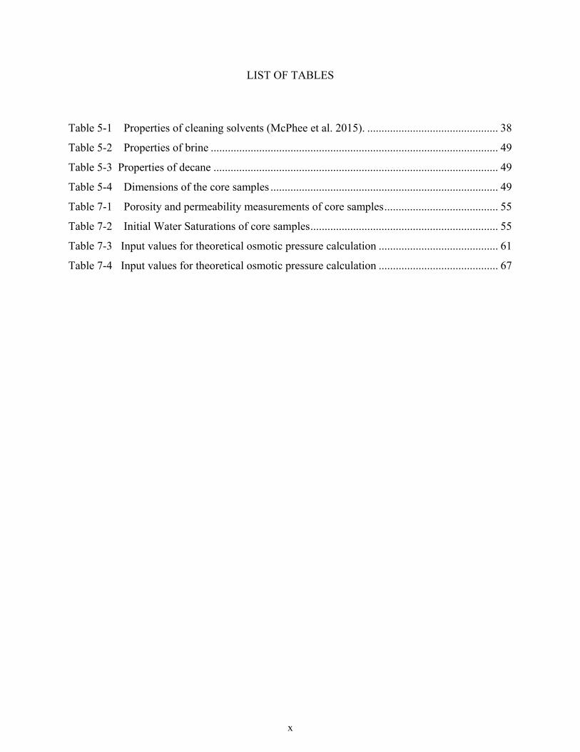
LIST OF TABLES

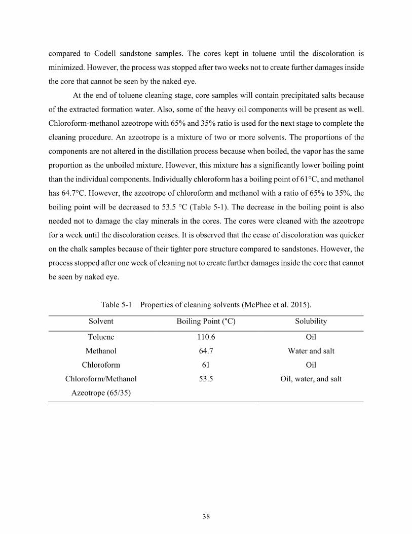
Table 5-1 Properties of cleaning solvents (McPhee et al. 2015). .............................................. 38 

Table 5-2 Properties of brine ..................................................................................................... 49 

Table 5-3 Properties of decane .................................................................................................... 49 

Table 5-4 Dimensions of the core samples ................................................................................ 49 

Table 7-1 Porosity and permeability measurements of core samples ........................................ 55 

Table 7-2 Initial Water Saturations of core samples .................................................................. 55 

Table 7-3 Input values for theoretical osmotic pressure calculation .......................................... 61 

Table 7-4 Input values for theoretical osmotic pressure calculation .......................................... 67 

xi

LIST OF SYMBOLS - ENGLISH

B constant for each solvent that is related to the deviations of the system from the ideal solution laws

c Molar concentration

I ionic strength

l length of the sample

M molality of the electrolyte

MW Molecular weight of solvent

n rotation speed

n Number of moles p Pressure

cp Capillary pressure

nwp Non-wetting phase pressure

wp Wetting phase pressure

R Gas constant

r distance from the center of rotation

2r distance from the center of rotation to outer face of the core

s Solvent

oS Saturation of oil

wS Saturation of water

,w irrS Irreducible water saturation

T Temperature, T

x Mole fraction

z z - valences of ions

xii

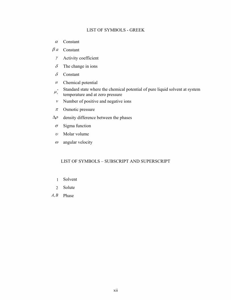
LIST OF SYMBOLS - GREEK

Constant

a Constant Activity coefficient

The change in ions

Constant Chemical potential

*s Standard state where the chemical potential of pure liquid solvent at system

temperature and at zero pressure v Number of positive and negative ions

Osmotic pressure

density difference between the phases

Sigma function

Molar volume

angular velocity

LIST OF SYMBOLS – SUBSCRIPT AND SUPERSCRIPT

1 Solvent

2 Solute A B, Phase

xiii

ACKNOWLEDGEMENTS

I want to express my sincere gratitude to my advisor Dr. Hossein Kazemi for his guidance

and insight throughout the thesis study and during my studies in Colorado School of Mines. He

inspired me to become an independent researcher and experimentalist. It has been a great privilege

and pleasure to work with him. Without his expert advice and support it would not have been

possible to finish this work. I would also like to thank to my committee members, Dr. Erdal Ozkan

and Dr. Azra Tutuncu who helped me to understand the reservoir engineering concept and enrich

my ideas. I would like to extend my gratitude to my minor advisor Dr. Steve Sonnenberg whose

technical expertise greatly contributed to improve and broaden my scientific knowledge in

petroleum geology.

I am also thankful for my company, Schlumberger, for granting me educational leave of

absence to pursue my MS degree. I am thankful to all my colleagues in MCERS with special thanks

to Denise Winn-Bower for her support and assistance throughout my MS study.

I would also like to thank my friends who helped me to cheer up and get through the hard

times; Jason Carey, Sergio Suarez-Fernandez, and many others.

Needless to say, I am very grateful to my parents, my sister Ilkay and brother-in-law Erdinc,

it would not be possible without your love and source of energy.

1

INTRODUCTION

This thesis presents a practical technique to measure osmotic pressure in Niobrara chalk

and Codell sandstone cores using an ultra-high-speed centrifuge. In this chapter, I will present the

research objective, a brief description of methodology, and research contributions.

1.1 Problem Statement

Hydrocarbon recovery from unconventional reservoirs is very low; that is, maximum of

ten percent. Therefore, improved methods to increase the oil production from shale reservoirs are

needed. Classical waterflooding in unconventional reservoirs is not plausible because of the pore

sizes; however, creating osmotic pressure by salinity contrast can cause a counter-current flow of

oil and water by imbibing water to expel oil. Despite this apparent and potential benefit of osmotic

pressure to make waterflooding feasible in shale reservoirs, waterflooding shale reservoirs is

essentially impossible because of the tight matrix. The latter is the motivation for the research in

this thesis.

Large salinity contrasts between stimulation fluids and formation lead to large osmotic

pressures. This could improve the extraction of oil from the tight matrix of unconventional shale

reservoirs. Thus, the potential of osmotic pressure created as a function of salinity contrast in such

formations should be investigated. A related issue is gas trapping in many water drive gas

reservoirs. This thesis also documents the use of the centrifuge to measure trapped gas saturation.

The aforementioned notions could lead to standard laboratory techniques for measuring

osmotic pressure for use in shale reservoirs and trapped gas saturation in water drive gas reservoirs.

This thesis embarks on two different ideas: (1) Determining osmotic pressure in shale core

samples, and (2) Enhancing oil recovery by low-salinity brine osmotic force to displace oil.

1.2 Objectives

The objectives of this research are:

(i) Investigate the potential of oil production improvement using the osmotic pressure

concept for unconventional shale reservoirs.

2

(ii) Investigate the trapped gas saturation using standard trapped gas saturation

measurements.

1.3 Methodology

Experimental work was performed using ultra-high-speed centrifuge with formation brine

and low salinity brine for cores from Niobrara chalk and Codell sandstone formations to examine

the effect of salinity contrast. Initially, CMS-300 device was used to estimate the pore volume,

porosity and permeability values of the cores. Then, the centrifuge was used to saturate the cores

with formation brine. Following core saturation, the cores were drained using decane in a drainage

setup and then forced imbibition process was performed with low salinity brine using an imbibition

setup. In between drainage and forced imbibition processes, spontaneous imbibition was

performed with low salinity brine.

Trapped gas measurements were performed using ultra-high-speed centrifuge with

formation brine and air by using cores from Bulo Bulo Field, Robore-III formation, Bolivia to

examine the trapped gas saturation. Initially, the CMS-300 system was used to estimate the pore

volume, porosity and permeability values of the cores. Then, the centrifuge was used to saturate

the cores with formation brine. In contrast to osmosis experiments, for the drainage process, the

formation brine saturated core was drained with air followed by forced imbibition process, in

which the formation brine was injected. In between drainage and forced imbibition processes, the

spontaneous imbibition was performed with formation brine using the under weighting balance

setup.

1.4 Research Contributions

In this research, the osmotic pressure created via salinity contrast in unconventional shale

reservoirs was measured using ultra-high-speed centrifuge experiments. High-speed centrifuge is

a novel technique to rapidly measure osmotic pressure in very low permeability cores.

Furthermore, it was observed that the osmotic pressure could improve the oil production from such

tight matrix formations. Consequently, the imbibition force to determined the EOR fraction was

quantified. Moreover, the membrane efficiency was calculated.

3

In addition to quantifying osmotic pressure and the EOR by osmosis, I also embarked on

quantifying the magnitude of trapped gas saturation when water enters a core.

1.5 Thesis Organization

This thesis has eight chapters.

Chapter 1 states the purpose, motivation, objectives, methodology, and the contributions

of the research.

Chapter 2 presents the relevant publications that focus on the effects of low salinity brine

on conventional reservoirs and theories on the effect of low salinity brine on production.

Chapter 3 presents an overview of the osmotic pressure, focusing on the semi-permeable

behavior of clays.

Chapter 4 presents a geological overview of the Niobrara chalk and Codell sandstone

formations.

Chapter 5 discusses the experimental methods. Core cleaning process, porosity and

permeability measurements using CMS-300, drainage, and imbibition process using ultra-high-

speed centrifuge are explained.

Chapter 6 presents the literature review on trapped gas saturation, a geological overview

of Robore III formation, and discusses the experimental methods for trapped gas measurements.

Chapter 7 presents results of osmotic pressure experiments. The discussion of the results

is also included in this chapter.

Chapter 8 presents the conclusions and recommendations of this research

4

EFFECT OF LOW SALINITY BRINE

The investigation on the effect of low salinity concentration brine on production dates back

to the 1940s. However, it did not attract the attention of researchers on the EOR/IOR aspect until

the 1990s. During the 90’s Morrow’s research on the effect of wettability on oil recovery led him

and his colleagues to focus on the effects of salinity on oil recovery. Their research on Berea

sandstone cores and cores from Prudhoe Bay, Alaska demonstrated the effect of brine salinity on

the wettability of the rock and oil recovery. Tang and Morrow (1999) generalized the necessary

conditions for the effect of low salinity to take place as; the presence of connate brine and initially

resided clay content in rock along with mixed wettability. These can be accepted as the first

screening efforts for low salinity mechanisms. However, further studies revealed that these

conditions are not sufficient to explain the effect of low salinity. Later on, various other laboratory

studies proved the possibility of oil recovery with low salinity flooding on oil recovery with

promising results which followed by the discussions on the original driving mechanism for the

technique.

This chapter presents the overview of the main theories of the effect of low salinity.

2.1 Overview of the Effect of Low Salinity Contrast

The main theories behind the effect of salinity contrast can be gathered under five

mechanisms; fines migration, pH increase, multicomponent ion exchange, double layer expansion,

and osmosis.

2.1.1 Fines Migration

Fines migration was the first mechanism that was proposed as a mechanism for oil recovery

with salinity contrast. Bernard (1967) performed experiments for injecting NaCl brine to Berea

sandstone cores and an outcrop core from Wyoming which had 1.2 % clay. According to this study,

the increase in recovery was due to the improved microscopic sweep efficiency induced by clay

swelling and plugging of pore throat by fines migration.

Fines migration also observed in the core samples during the low salinity flooding

experiments conducted by Tang and Morrow (1999). In these experiments, it was observed that

water took different flow paths due to the permeability reduction and increased differential

5

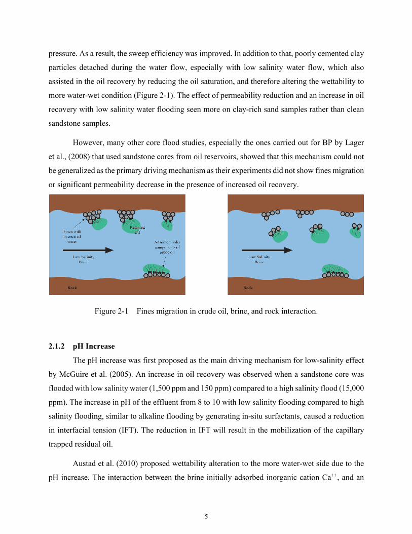
pressure. As a result, the sweep efficiency was improved. In addition to that, poorly cemented clay

particles detached during the water flow, especially with low salinity water flow, which also

assisted in the oil recovery by reducing the oil saturation, and therefore altering the wettability to

more water-wet condition (Figure 2-1). The effect of permeability reduction and an increase in oil

recovery with low salinity water flooding seen more on clay-rich sand samples rather than clean

sandstone samples.

However, many other core flood studies, especially the ones carried out for BP by Lager

et al., (2008) that used sandstone cores from oil reservoirs, showed that this mechanism could not

be generalized as the primary driving mechanism as their experiments did not show fines migration

or significant permeability decrease in the presence of increased oil recovery.

 

Figure 2-1 Fines migration in crude oil, brine, and rock interaction.

 

2.1.2 pH Increase

The pH increase was first proposed as the main driving mechanism for low-salinity effect

by McGuire et al. (2005). An increase in oil recovery was observed when a sandstone core was

flooded with low salinity water (1,500 ppm and 150 ppm) compared to a high salinity flood (15,000

ppm). The increase in pH of the effluent from 8 to 10 with low salinity flooding compared to high

salinity flooding, similar to alkaline flooding by generating in-situ surfactants, caused a reduction

in interfacial tension (IFT). The reduction in IFT will result in the mobilization of the capillary

trapped residual oil.

Austad et al. (2010) proposed wettability alteration to the more water-wet side due to the

pH increase. The interaction between the brine initially adsorbed inorganic cation Ca++, and an

6

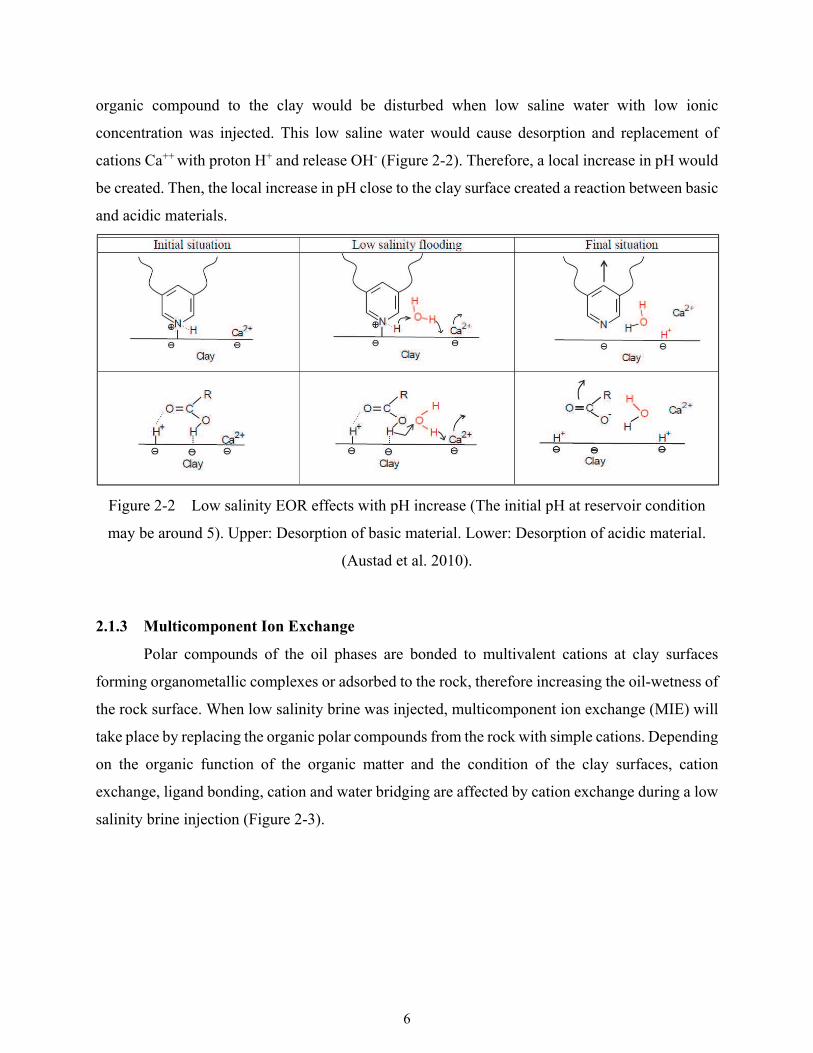
organic compound to the clay would be disturbed when low saline water with low ionic

concentration was injected. This low saline water would cause desorption and replacement of

cations Ca++ with proton H+ and release OH- (Figure 2-2). Therefore, a local increase in pH would

be created. Then, the local increase in pH close to the clay surface created a reaction between basic

and acidic materials.

Figure 2-2 Low salinity EOR effects with pH increase (The initial pH at reservoir condition

may be around 5). Upper: Desorption of basic material. Lower: Desorption of acidic material.

(Austad et al. 2010).

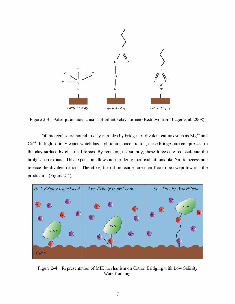
2.1.3 Multicomponent Ion Exchange

Polar compounds of the oil phases are bonded to multivalent cations at clay surfaces

forming organometallic complexes or adsorbed to the rock, therefore increasing the oil-wetness of

the rock surface. When low salinity brine was injected, multicomponent ion exchange (MIE) will

take place by replacing the organic polar compounds from the rock with simple cations. Depending

on the organic function of the organic matter and the condition of the clay surfaces, cation

exchange, ligand bonding, cation and water bridging are affected by cation exchange during a low

salinity brine injection (Figure 2-3).

7

 Figure 2-3 Adsorption mechanisms of oil into clay surface (Redrawn from Lager et al. 2008).

Oil molecules are bound to clay particles by bridges of divalent cations such as Mg++ and

Ca++. In high salinity water which has high ionic concentration, these bridges are compressed to

the clay surface by electrical forces. By reducing the salinity, these forces are reduced, and the

bridges can expand. This expansion allows non-bridging monovalent ions like Na+ to access and

replace the divalent cations. Therefore, the oil molecules are then free to be swept towards the

production (Figure 2-4).

Figure 2-4 Representation of MIE mechanism on Cation Bridging with Low Salinity Waterflooding.

8

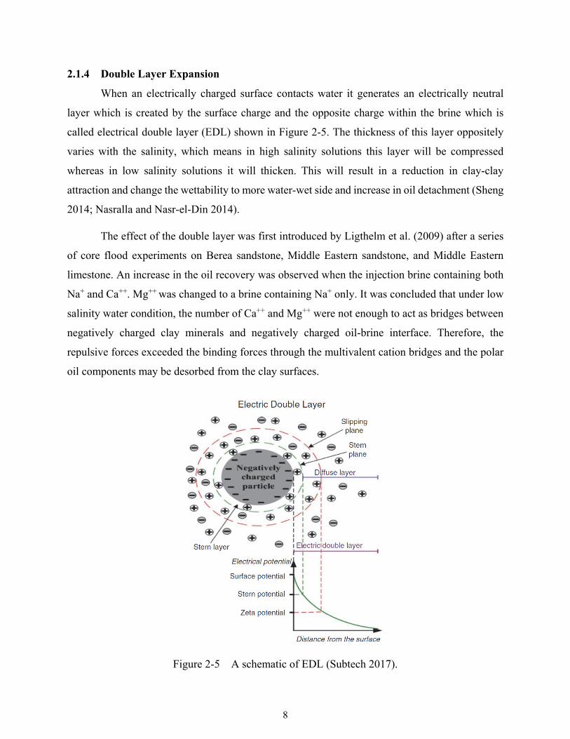
2.1.4 Double Layer Expansion

When an electrically charged surface contacts water it generates an electrically neutral

layer which is created by the surface charge and the opposite charge within the brine which is

called electrical double layer (EDL) shown in Figure 2-5. The thickness of this layer oppositely

varies with the salinity, which means in high salinity solutions this layer will be compressed

whereas in low salinity solutions it will thicken. This will result in a reduction in clay-clay

attraction and change the wettability to more water-wet side and increase in oil detachment (Sheng

2014; Nasralla and Nasr-el-Din 2014).

The effect of the double layer was first introduced by Ligthelm et al. (2009) after a series

of core flood experiments on Berea sandstone, Middle Eastern sandstone, and Middle Eastern

limestone. An increase in the oil recovery was observed when the injection brine containing both

Na+ and Ca++. Mg++ was changed to a brine containing Na+ only. It was concluded that under low

salinity water condition, the number of Ca++ and Mg++ were not enough to act as bridges between

negatively charged clay minerals and negatively charged oil-brine interface. Therefore, the

repulsive forces exceeded the binding forces through the multivalent cation bridges and the polar

oil components may be desorbed from the clay surfaces.

 

Figure 2-5 A schematic of EDL (Subtech 2017).

9

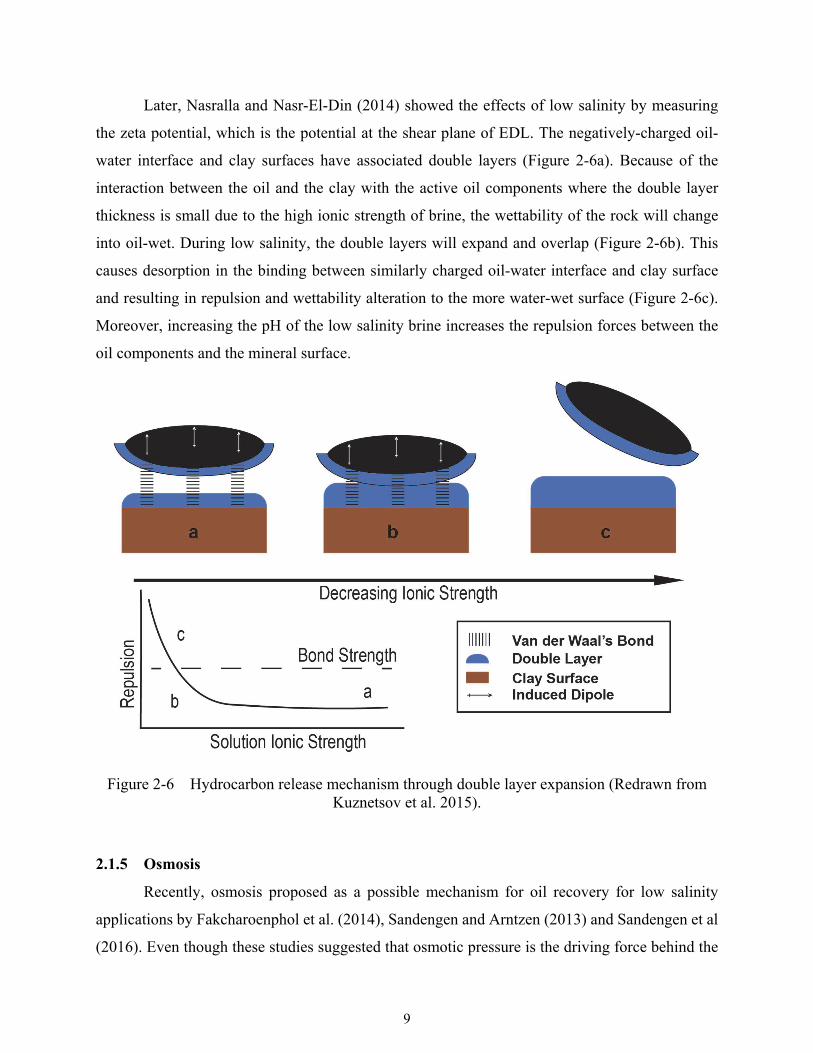
Later, Nasralla and Nasr-El-Din (2014) showed the effects of low salinity by measuring

the zeta potential, which is the potential at the shear plane of EDL. The negatively-charged oil-

water interface and clay surfaces have associated double layers (Figure 2-6a). Because of the

interaction between the oil and the clay with the active oil components where the double layer

thickness is small due to the high ionic strength of brine, the wettability of the rock will change

into oil-wet. During low salinity, the double layers will expand and overlap (Figure 2-6b). This

causes desorption in the binding between similarly charged oil-water interface and clay surface

and resulting in repulsion and wettability alteration to the more water-wet surface (Figure 2-6c).

Moreover, increasing the pH of the low salinity brine increases the repulsion forces between the

oil components and the mineral surface.

 

Figure 2-6 Hydrocarbon release mechanism through double layer expansion (Redrawn from Kuznetsov et al. 2015).

 

2.1.5 Osmosis

Recently, osmosis proposed as a possible mechanism for oil recovery for low salinity

applications by Fakcharoenphol et al. (2014), Sandengen and Arntzen (2013) and Sandengen et al

(2016). Even though these studies suggested that osmotic pressure is the driving force behind the

10

low salinity effect, they differ on the proposed semi-permeable membrane for osmosis to take

place. Fakcharoenphol et al. (2014) suggested that the rock matrix, in particular, the shales,

behaves as a semi-permeable membrane. The experiment carried out as low and high salinity

imbibition using sandstone core samples from Middle Bakken formation. In addition to the

experiments, a mathematical model was presented for a multi-phase, chemical osmosis flow model

for hydrocarbon bearing shale formations by defining osmotic pressure as a function of salt

concentration and the mathematical model was tested by validating the osmotic pressures

measured in a shale sample experiment conducted by Takeda et al. (2012).

Sandengen et al. (2016) proposed that oil behaves as a semi-permeable membrane that

transports water but not the ions based on the description of Su et al. (2010) on the behavior of oil.

The driving force is the activity of the water, and water is thought to be passing through the oil

and encounter with connate water which has higher salinity, and therefore connate water will swell

and move the surrounding oil. The enclosure of water filled cavities with oil is required so that oil

saturation would be high. Also, a wide pore size distribution would be beneficial. As a result, water

will be moved from the water transporting large pores and into the less conductive network of

small pores.

The focus of this research is the measurement of osmotic pressure. Therefore, osmosis and

osmotic pressure will be covered in more detail in Chapter 3.

11

OSMOSIS

Osmosis is the movement of solvent particles across a semipermeable membrane from

a dilute solution into a concentrated solution. The solvent moves to dilute the concentrated

solution and equalize concentration on both sides of the membrane.

This chapter includes (1) overview of osmosis concept and historical background, (2)

clay mineralogy, and (3) semi-permeable behavior of clays.

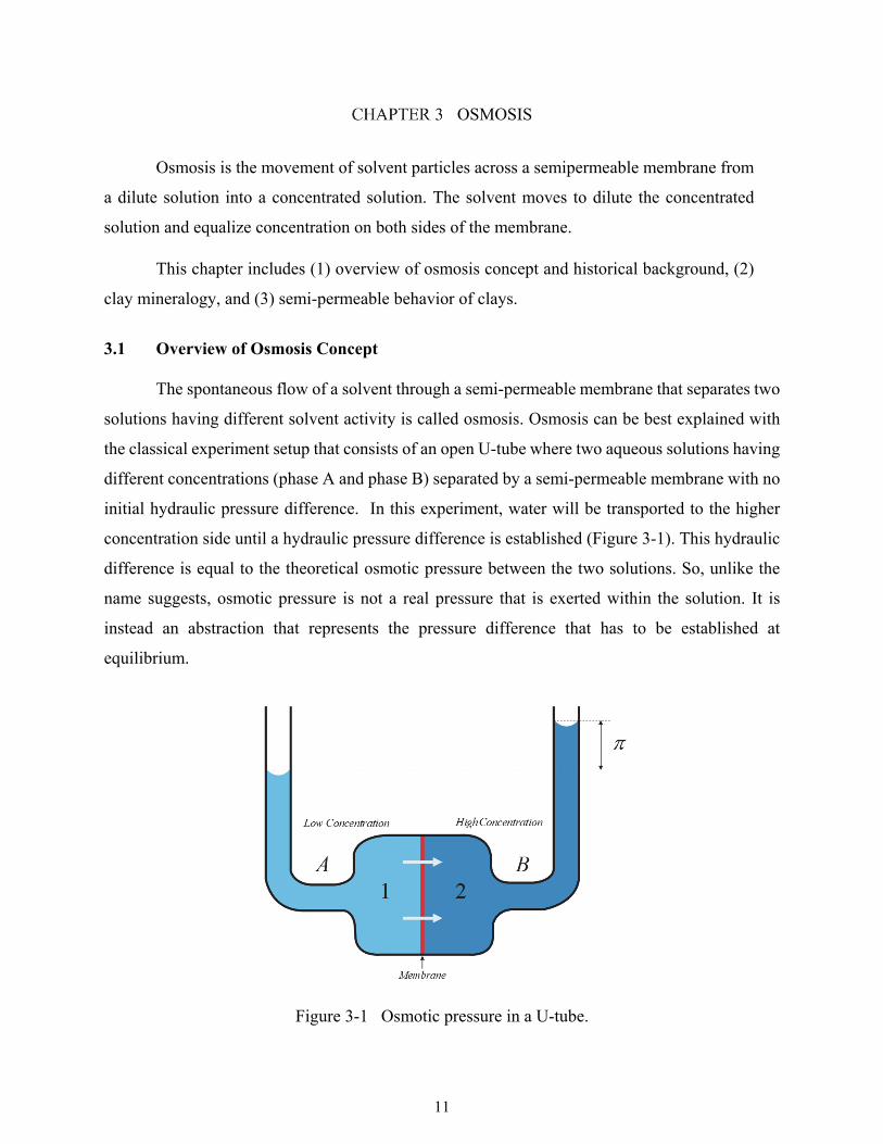
3.1 Overview of Osmosis Concept

The spontaneous flow of a solvent through a semi-permeable membrane that separates two

solutions having different solvent activity is called osmosis. Osmosis can be best explained with

the classical experiment setup that consists of an open U-tube where two aqueous solutions having

different concentrations (phase A and phase B) separated by a semi-permeable membrane with no

initial hydraulic pressure difference. In this experiment, water will be transported to the higher

concentration side until a hydraulic pressure difference is established (Figure 3-1). This hydraulic

difference is equal to the theoretical osmotic pressure between the two solutions. So, unlike the

name suggests, osmotic pressure is not a real pressure that is exerted within the solution. It is

instead an abstraction that represents the pressure difference that has to be established at

equilibrium.

Figure 3-1 Osmotic pressure in a U-tube.

12

3.1.1 Historical Background of Osmosis

The osmotic pressure was first described by Abbe Nollet in 1748. However first direct

measurements were conducted more than a century later by a botanist, Pfeffer in 1877 by using

sugar solutions. He noted that membranes appeared to permit passage of water while restraining

the passage of solutes. In 1861, Thomas Graham documented that transfer of certain substances is

slower in diffusion while he was working on dialyzers. He called these substances colloids. He

formulated the theory that these dissolved substances exert a pressure which is analogous of gas

under certain conditions. After analyzing the results of the experiments of Pfeffer, Van’t Hoff also

noted the analogy between the data and the perfect gas law (Farrington and Daniels 1979).

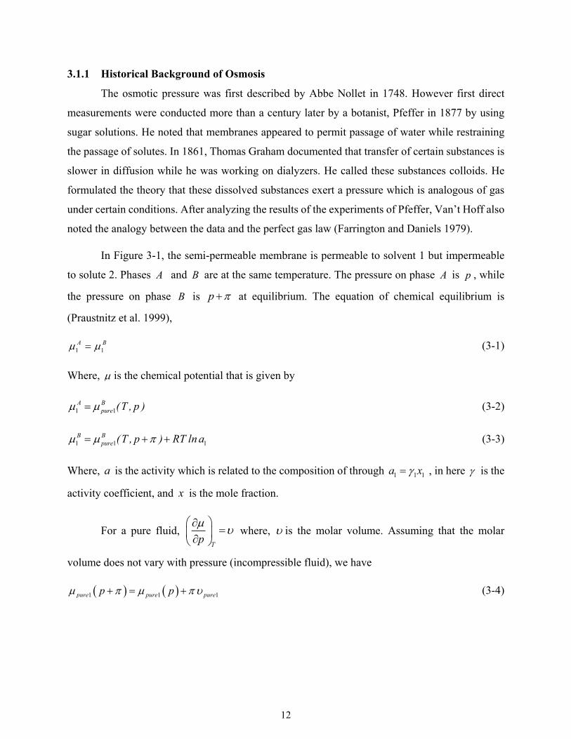
In Figure 3-1, the semi-permeable membrane is permeable to solvent 1 but impermeable

to solute 2. Phases A and B are at the same temperature. The pressure on phase A is p , while

the pressure on phase B is p at equilibrium. The equation of chemical equilibrium is

(Praustnitz et al. 1999),

1 1A B (3-1)

Where, is the chemical potential that is given by

1 1A B

pure (T , p ) (3-2)

1 1 1B B

pure (T , p ) RT ln a (3-3)

Where, a is the activity which is related to the composition of through 1 1 1a x , in here is the

activity coefficient, and x is the mole fraction.

For a pure fluid, T

p

where, is the molar volume. Assuming that the molar

volume does not vary with pressure (incompressible fluid), we have

1 1 1pure pure purep p (3-4)

13

Equation 3-2 can be rewritten as

11

pureln a

RT

(3-5)

If the solution in phase B is dilute, 1x is close to unity; in that event 1 is also close to unity and

Eq. 3-5 becomes,

11

pureln x

RT

(3-6)

When 2 1 2 21 1x ,ln x ln( x ) x , Eq. 3-6 becomes

1 2pure x RT (3-7)

Because 22 2 1 2

1

1 nx , n n and x

n Eq. 3-7 becomes,

2V n RT (3-8)

Where, 1 1pureV n is the total volume available to 2n moles of solute.

Equation 3-8 is termed as ideal osmotic pressure equation or Van’t Hoff equation. The ideal

osmotic pressure relation was derived for systems where membrane permeability is not ion

selective or for solutions of non-electrolytes. However, the osmotic pressure relation becomes

more complex in case of the presence of aforementioned conditions. This condition can be

described by a U-tube set up consisting of a chamber that is divided into two parts by a membrane

that is ion selective, which means the membrane allows some of the ions to flow through while

inhibiting others (Figure 3-2). In this case, it is necessary to satisfy the electrical neutrality criteria

for each of the phases in the chamber in addition to the usual Gibbs equations for equality of

chemical potentials (Praustnitz et al. 1999).

14

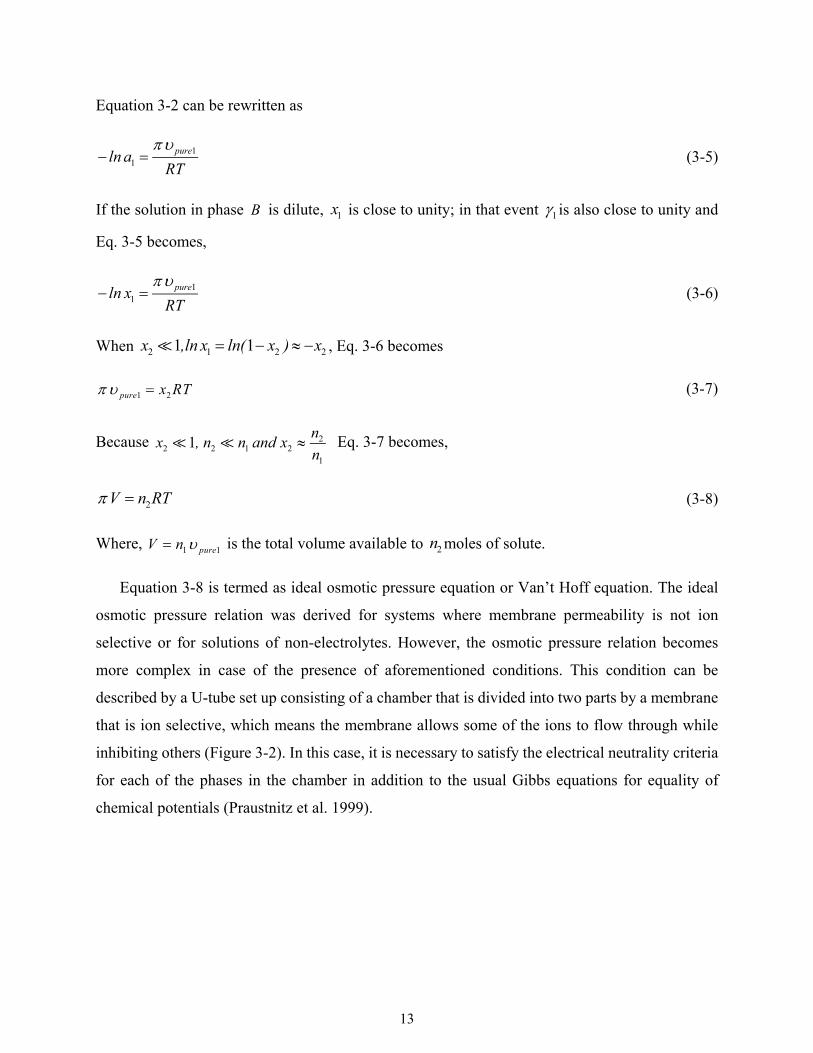
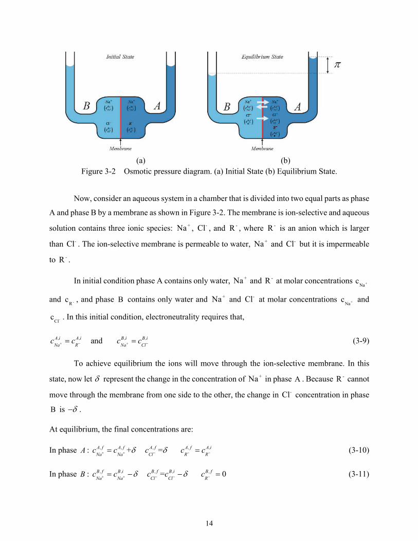
  (a) (b) 

Figure 3-2 Osmotic pressure diagram. (a) Initial State (b) Equilibrium State.

Now, consider an aqueous system in a chamber that is divided into two equal parts as phase

A and phase B by a membrane as shown in Figure 3-2. The membrane is ion-selective and aqueous

solution contains three ionic species: +Na , -Cl , and -R , where -R is an anion which is larger

than -Cl . The ion-selective membrane is permeable to water, +Na and -Cl but it is impermeable

to -R .

In initial condition phase A contains only water, +Na and -R at molar concentrations +Nac

and -Rc , and phase B contains only water and +Na and -Cl at molar concentrations +Na

c and

-Clc . In this initial condition, electroneutrality requires that,

and A,i A,i B ,i B ,i

Na R Na Clc c c c (3-9)

To achieve equilibrium the ions will move through the ion-selective membrane. In this

state, now let represent the change in the concentration of +Na in phase A . Because -R cannot

move through the membrane from one side to the other, the change in -Cl concentration in phase

B is .

At equilibrium, the final concentrations are:

In phase A : + = A, f A, f A, f A, f A,i

Na Na Cl R Rc c c c c (3-10)

In phase B : = 0B, f B ,i B , f B ,i B , f

Na Na Cl Cl Rc c c c c (3-11)

15

The equation of chemical equilibrium for the solvent is,

A B

s s (3-12)

Where, s represents solvent.

The relationship between the chemical potential, pressure, and activity can be denoted by

* lnA A A

s s s sp RT a (3-13)

* lnB B B

s s s sp RT a (3-14)

Where, *s is the standard state where the chemical potential of pure liquid solvent at system

temperature and zero pressure.

Substituting Equations 3-13 and 3-14 into Equation 3-12 yields,

lnB

A B s

A

s s

aRTp p

a

(3-15)

The activity coefficient of water in an aqueous Potassium Chloride KCl solution using

Debye-Huckel limiting law,

2 2 21

3 2H O H O H O KCl -

Iln( x ) -MW v M - z z I a I

(3-16)

Where,

31 11 2 1

1y y ln y

y y

(3-17)

Here, MW is the molecular weight of the solvent, v  the number of positive and negative ions, M

molality of the electrolyte, z z -  valences of ions, I ionic strength, sigma function, and , 

a ,  constants.

The measured osmotic pressure obtained from an experiment by using a nonideal

membrane is different from the thermodynamically predicted value by using Equation 3-15

(Staverman 1952). The comparison of the theoretical and measured values of osmotic pressure

will display the membrane efficiency of the media that is used as a semipermeable membrane.

16

Here, the membrane efficiency defines the ability of the media to deter ion movement when

interacting with ionic fluids. The membrane efficiency will be equal to one if all ionic movement

is stopped. Therefore, the media is a perfect semi-permeable membrane. The earlier studies to

determine the membrane efficiency of shale samples showed that this value ranges between 0.18%

to 4.23% (Zhang et al. 2008).

First laboratory studies on geological materials and the effect of osmosis were done by De

Sitter (1947). He suggested that argillaceous sediments have the ability to act as a semi-permeable

membrane to explain the salinity changes in subsurface waters in depth. Also, White (1957)

proposed that the connate water salinities are the result of the filtering of salt ions by semi-

permeable membranes.

In 1959, Berry determined the reason for the apparent hydrodynamic sink in the San Juan

basin as osmosis. Kemper (1960), and also in another study by McKelvey and Milne (1962)

showed the exclusion of the salt ions by using a clay membrane. On a follow-up study, Milne et

al. (1964) conducted experiments to show the inhibition of salt transmission by applying a pressure

gradient and using bentonite membranes. In 1961, Hill proposed that subsurface pressure

anomalies in the San Juan basin of New Mexico and the pressure anomalies in Alberta, Canada,

are the result of osmosis. Also, Zen and Hanshaw (1964) suggested that high pore pressures related

with osmotic pressure may trigger the overthrust faulting. They proposed that in specific areas

where the negative charge on the walls of colloidal sized pores which anions are entering restricts

the transfer of dissolved salts but allowing the water to pass. Therefore, in this system, the colloidal

sized small pores are acting as a semi-permeable membrane to allow the osmosis to occur.

Membrane behavior of clays has been known for a long time. Kharaka and Berry (1973)

have shown that the hyperfiltration efficiency is a function of pressure and concentration gradients,

temperature, membrane porosity, and type of ion. Another study by Wood (1976) suggested that

the some of the dominant ionic species in the aquifer system of Saginaw, Michigan may be

controlled by hyperfiltration by the help of the clay minerals in the formation.

Therefore, the theory of clays acting as semi-permeable membranes is used to explain the

salinities and the chemical compositions of formation waters that cannot be explained solely by

water-rock interactions. Thus, the mineralogy of clays is a crucial aspect to consider when

discussing the semi-permeable membrane behavior of clay platelets.

17

3.2 Clay Mineralogy

Clay minerals are a combination of two units of atomic lattices, octahedron and silica

tetrahedrons. They are characterized by the arrangement of the sheets that are formed by these

atomic lattices and isomorphous substitution within the crystal’s structure. They occur in small

sizes, and they have negative charges which are balanced by the adsorption of cations from the

solutions (Mitchell and Soga 2005, Grim 1968).

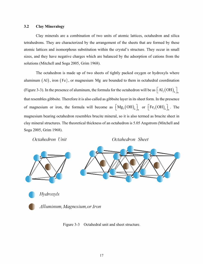
The octahedron is made up of two sheets of tightly packed oxygen or hydroxyls where

aluminum Al , iron Fe , or magnesium Mg are bounded to them in octahedral coordination

(Figure 3-3). In the presence of aluminum, the formula for the octahedron will be as 2 6 nAl OH

that resembles gibbsite. Therefore it is also called as gibbsite layer in its sheet form. In the presence

of magnesium or iron, the formula will become as 3 6 nMg OH or 3 6 n

Fe OH . The

magnesium bearing octahedron resembles brucite mineral, so it is also termed as brucite sheet in

clay mineral structures. The theoretical thickness of an octahedron is 5.05 Angstrom (Mitchell and

Soga 2005, Grim 1968).

 

Figure 3-3 Octahedral unit and sheet structure.  

18

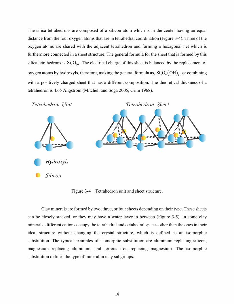
The silica tetrahedrons are composed of a silicon atom which is in the center having an equal

distance from the four oxygen atoms that are in tetrahedral coordination (Figure 3-4). Three of the

oxygen atoms are shared with the adjacent tetrahedron and forming a hexagonal net which is

furthermore connected in a sheet structure. The general formula for the sheet that is formed by this

silica tetrahedrons is 4 10Si O . The electrical charge of this sheet is balanced by the replacement of

oxygen atoms by hydroxyls, therefore, making the general formula as, 4 6 4Si O OH , or combining

with a positively charged sheet that has a different composition. The theoretical thickness of a

tetrahedron is 4.65 Angstrom (Mitchell and Soga 2005, Grim 1968).

 

Figure 3-4 Tetrahedron unit and sheet structure.

 

Clay minerals are formed by two, three, or four sheets depending on their type. These sheets

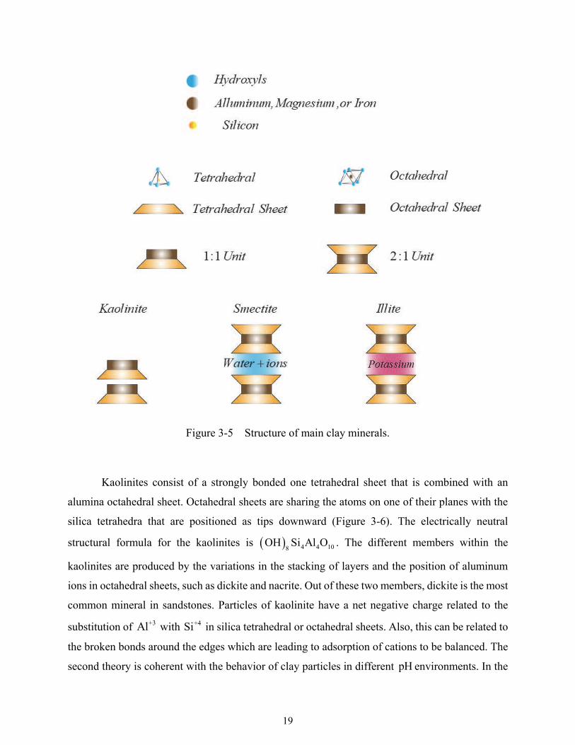
can be closely stacked, or they may have a water layer in between (Figure 3-5). In some clay

minerals, different cations occupy the tetrahedral and octahedral spaces other than the ones in their

ideal structure without changing the crystal structure, which is defined as an isomorphic

substitution. The typical examples of isomorphic substitution are aluminum replacing silicon,

magnesium replacing aluminum, and ferrous iron replacing magnesium. The isomorphic

substitution defines the type of mineral in clay subgroups.

19

Figure 3-5 Structure of main clay minerals.

Kaolinites consist of a strongly bonded one tetrahedral sheet that is combined with an

alumina octahedral sheet. Octahedral sheets are sharing the atoms on one of their planes with the

silica tetrahedra that are positioned as tips downward (Figure 3-6). The electrically neutral

structural formula for the kaolinites is 4 4 108OH Si Al O . The different members within the

kaolinites are produced by the variations in the stacking of layers and the position of aluminum

ions in octahedral sheets, such as dickite and nacrite. Out of these two members, dickite is the most

common mineral in sandstones. Particles of kaolinite have a net negative charge related to the

substitution of +3Al with +4Si in silica tetrahedral or octahedral sheets. Also, this can be related to

the broken bonds around the edges which are leading to adsorption of cations to be balanced. The

second theory is coherent with the behavior of clay particles in different pH environments. In the

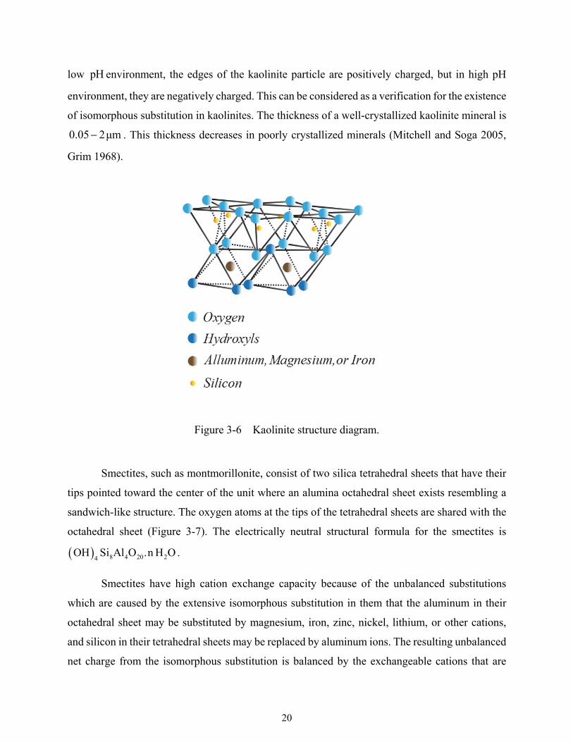
20

low pH environment, the edges of the kaolinite particle are positively charged, but in high pH

environment, they are negatively charged. This can be considered as a verification for the existence

of isomorphous substitution in kaolinites. The thickness of a well-crystallized kaolinite mineral is

0.05 2μm . This thickness decreases in poorly crystallized minerals (Mitchell and Soga 2005,

Grim 1968).

 

Figure 3-6 Kaolinite structure diagram.

 

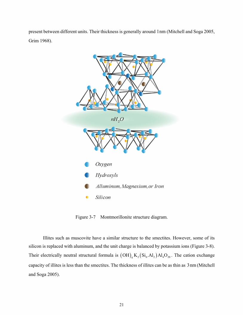
Smectites, such as montmorillonite, consist of two silica tetrahedral sheets that have their

tips pointed toward the center of the unit where an alumina octahedral sheet exists resembling a

sandwich-like structure. The oxygen atoms at the tips of the tetrahedral sheets are shared with the

octahedral sheet (Figure 3-7). The electrically neutral structural formula for the smectites is

8 4 20 24OH Si Al O .n H O .

Smectites have high cation exchange capacity because of the unbalanced substitutions

which are caused by the extensive isomorphous substitution in them that the aluminum in their

octahedral sheet may be substituted by magnesium, iron, zinc, nickel, lithium, or other cations,

and silicon in their tetrahedral sheets may be replaced by aluminum ions. The resulting unbalanced

net charge from the isomorphous substitution is balanced by the exchangeable cations that are

21

present between different units. Their thickness is generally around 1nm (Mitchell and Soga 2005,

Grim 1968).

 

Figure 3-7 Montmorillonite structure diagram.

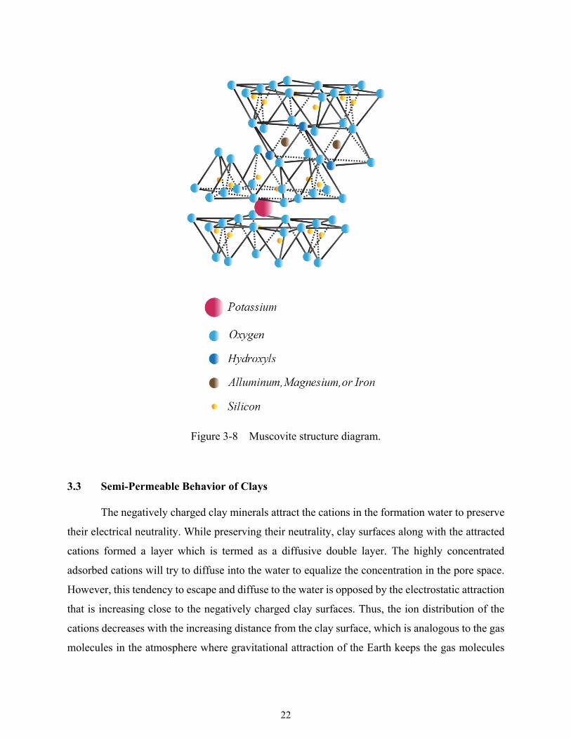
Illites such as muscovite have a similar structure to the smectites. However, some of its

silicon is replaced with aluminum, and the unit charge is balanced by potassium ions (Figure 3-8).

Their electrically neutral structural formula is 2 6 2 4 204OH K Si .Al Al O . The cation exchange

capacity of illites is less than the smectites. The thickness of illites can be as thin as 3nm (Mitchell

and Soga 2005).

22

 

Figure 3-8 Muscovite structure diagram.

3.3 Semi-Permeable Behavior of Clays

The negatively charged clay minerals attract the cations in the formation water to preserve

their electrical neutrality. While preserving their neutrality, clay surfaces along with the attracted

cations formed a layer which is termed as a diffusive double layer. The highly concentrated

adsorbed cations will try to diffuse into the water to equalize the concentration in the pore space.

However, this tendency to escape and diffuse to the water is opposed by the electrostatic attraction

that is increasing close to the negatively charged clay surfaces. Thus, the ion distribution of the

cations decreases with the increasing distance from the clay surface, which is analogous to the gas

molecules in the atmosphere where gravitational attraction of the Earth keeps the gas molecules

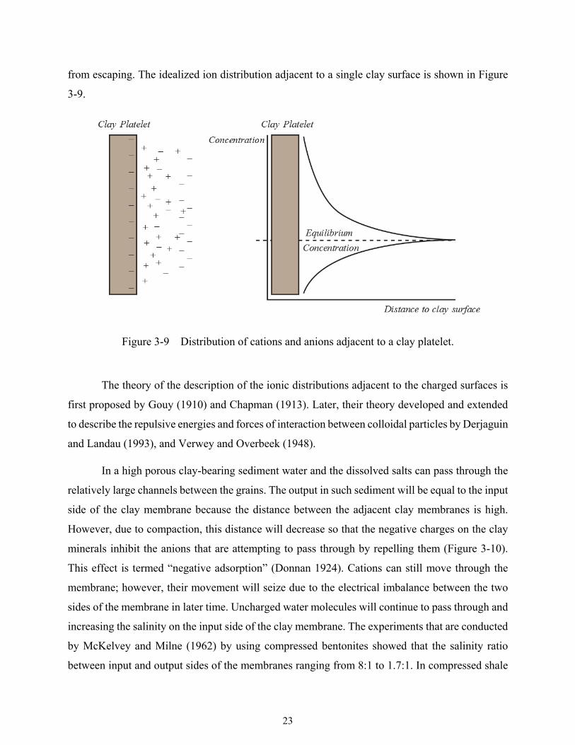
23

from escaping. The idealized ion distribution adjacent to a single clay surface is shown in Figure

3-9.

 

Figure 3-9 Distribution of cations and anions adjacent to a clay platelet.

 

The theory of the description of the ionic distributions adjacent to the charged surfaces is

first proposed by Gouy (1910) and Chapman (1913). Later, their theory developed and extended

to describe the repulsive energies and forces of interaction between colloidal particles by Derjaguin

and Landau (1993), and Verwey and Overbeek (1948).

In a high porous clay-bearing sediment water and the dissolved salts can pass through the

relatively large channels between the grains. The output in such sediment will be equal to the input

side of the clay membrane because the distance between the adjacent clay membranes is high.

However, due to compaction, this distance will decrease so that the negative charges on the clay

minerals inhibit the anions that are attempting to pass through by repelling them (Figure 3-10).

This effect is termed “negative adsorption” (Donnan 1924). Cations can still move through the

membrane; however, their movement will seize due to the electrical imbalance between the two

sides of the membrane in later time. Uncharged water molecules will continue to pass through and

increasing the salinity on the input side of the clay membrane. The experiments that are conducted

by McKelvey and Milne (1962) by using compressed bentonites showed that the salinity ratio

between input and output sides of the membranes ranging from 8:1 to 1.7:1. In compressed shale

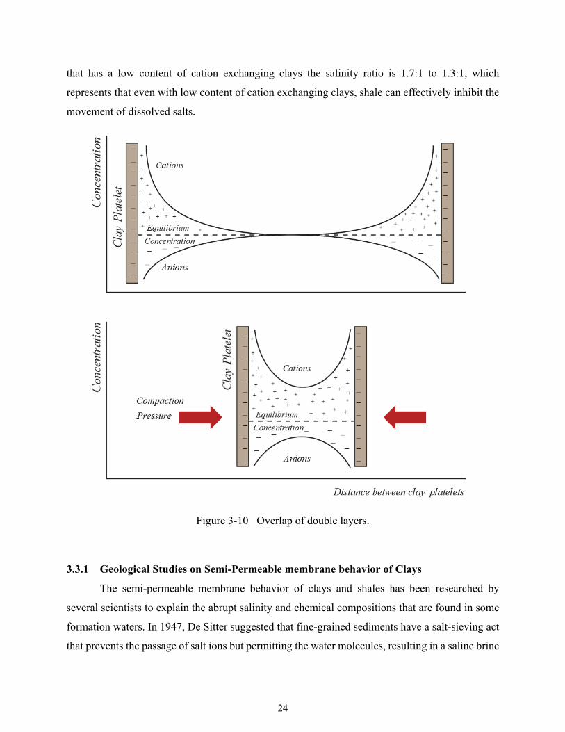
24

that has a low content of cation exchanging clays the salinity ratio is 1.7:1 to 1.3:1, which

represents that even with low content of cation exchanging clays, shale can effectively inhibit the

movement of dissolved salts.  

Figure 3-10 Overlap of double layers.

3.3.1 Geological Studies on Semi-Permeable membrane behavior of Clays

The semi-permeable membrane behavior of clays and shales has been researched by

several scientists to explain the abrupt salinity and chemical compositions that are found in some

formation waters. In 1947, De Sitter suggested that fine-grained sediments have a salt-sieving act

that prevents the passage of salt ions but permitting the water molecules, resulting in a saline brine

25

concentration. Hanshaw (1962) and Hanshaw and Coplen (1973) studied filtrated NaCl solutions

using compacted montmorillonite and illite membranes. Kharaka (1971) and Kaharaka and Berry

(1973) showed that the efficiency of a membrane is increased with the increase of compaction

pressure.

Biochemists suggested using osmotic pressure equations to determine the particle size and

molecular weight of particles in a protein solution separated by a semi-permeable membrane. A

modified Van’t Hoff equation (Eq. 3-18) is used to quantify the results of the experiments

conducted on protein solutions:

2cp RT Bc

MW ( ) (3-18)

Where, p is the osmotic pressure, R molar gas constant, T absolute temperature, c

concentration, MW average molecular weight, and B constant for each solvent that is related

to the deviations of the system from the ideal solution laws.

In later studies, it has been seen that there are osmotic force changes due to the movement

of ions that are added to the solution through the semi-permeable membrane. This phenomenon is

defined by Donnan. Thus it is called Donnan Membrane Equilibrium.

White (1965) made an analogy between the membrane behavior of clays, aforementioned

organic protein solutions and the Donnan membrane experiment. In Donnan membrane

experiment, the membrane has large pores that allow the passage of small ions but not permitting

the large ionized colloidal particles until an equilibrium is reached on both sides of the membrane.

Donnan conducted an experiment where he used a solution of a dye sodium salt called Congo Red,

that is used as a colloidal electrolyte, which is soaked into a NaCl solution but separated by a semi-

permeable membrane (Figure 3-11). The semi-permeable membrane that is used is impermeable

to Congo Red anions but permeable to all other ions that are present. It is observed that the +Na

and -Cl ions diffuse to the Congo Red solution until equilibrium is reached, later he used his

results to modify the Van’t Hoff equation to quantify this behavior (Hartman 1947).

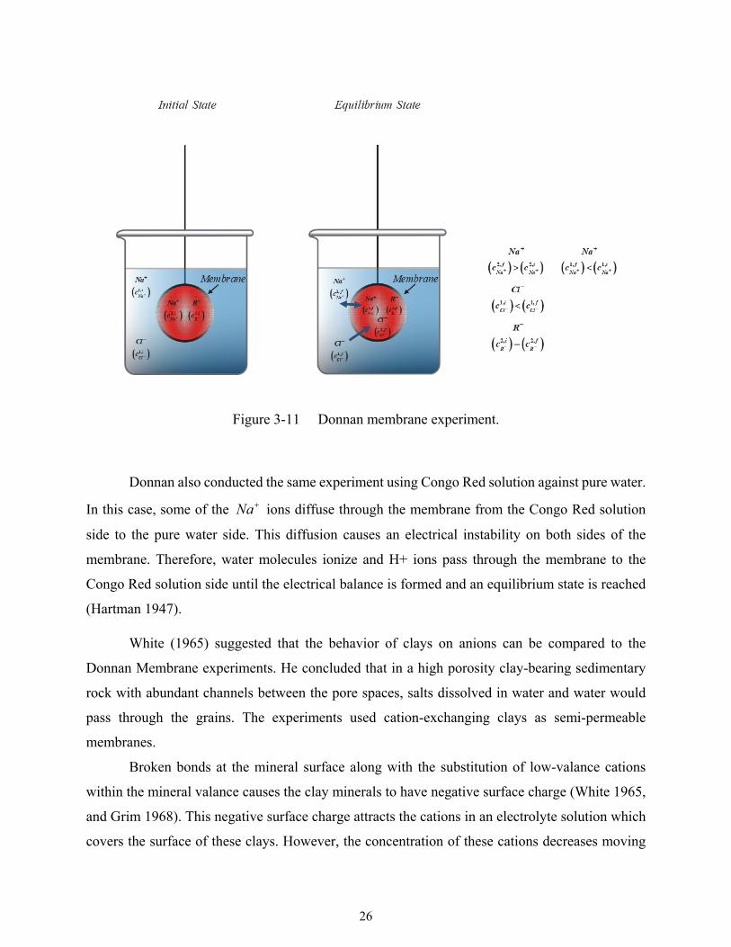
26

 

Figure 3-11 Donnan membrane experiment.

Donnan also conducted the same experiment using Congo Red solution against pure water.

In this case, some of the Na ions diffuse through the membrane from the Congo Red solution

side to the pure water side. This diffusion causes an electrical instability on both sides of the

membrane. Therefore, water molecules ionize and H+ ions pass through the membrane to the

Congo Red solution side until the electrical balance is formed and an equilibrium state is reached

(Hartman 1947).

White (1965) suggested that the behavior of clays on anions can be compared to the

Donnan Membrane experiments. He concluded that in a high porosity clay-bearing sedimentary

rock with abundant channels between the pore spaces, salts dissolved in water and water would

pass through the grains. The experiments used cation-exchanging clays as semi-permeable

membranes.

Broken bonds at the mineral surface along with the substitution of low-valance cations

within the mineral valance causes the clay minerals to have negative surface charge (White 1965,

and Grim 1968). This negative surface charge attracts the cations in an electrolyte solution which

covers the surface of these clays. However, the concentration of these cations decreases moving

27

away from the mineral surface into the pore. The double layer is composed of this negatively

charged layer of the mineral surface and cation that is attached to it.

The double layers in sandstones have little to no effect due to their relatively large sizes of

pore spaces compared to the thicknesses of the double layers. However, in clay-rich rocks, the

thickness of the double layers is comparable to the pore sizes, mainly due to the decrease of pore

spaces by compaction. The solutions in the pore spaces of a clay-rich rock that is compacted are

all influenced by the double layer as they start to overlap. This occurrence leads to the repel of the

anions to enter the clay pore but attract the cations in the solution. In later time, when cations that

are adjacent to clay surface become dominant ion species in the solution, they will start to repel

the cations from entering the clay pores as well. In this time, only electrically neutral water

molecules can pass through the pores. Hence, clays act as a semi-permeable membrane allowing

solvent components to pass but inhibiting the solutes. In this case, sandstones are not effective

membranes as they permit the passage of solutes as well. However, this is not the case for tight

sandstones due to their small pore sizes.

White (1965) describes that initially there is no perfect shale membrane in sedimentary

rocks, that they continue to allow some of the anions to escape through larger interconnected

openings. However, these interconnections sizes decrease in time as the compaction continues,

resulting in a nearly perfect membrane, and increasing the salinity on the input side of the

membrane. However, not all the pores are the same size, so in this case, the effect of still imperfect

membranes because of the escape routes due to larger pore spaces is the decrease of salinity at

some parts of the sedimentary rocks where larger pores exist. So, the salinity of brine in pore

spaces of shale may differ in salinity depending on the amount of adsorbed low salinity water.

In sedimentary basins, salinity increases with age. However, when the sedimentation is

uplifted after the end of the burial, the decrease in porosity will stop and even can be reversed as

compaction decreases. In this case, the system is not dominated anymore by the overburden stress,

but with hydrostatic pressure. Then, in this system, meteoric water flushes out the existing high

saline brines. However, it is also noted that the higher parts of the hydrologic system may provide

the energy needed for the salt-sieving. Therefore, the salinity in some parts of the system may

continue to increase.

28

Another discussion on the literature states that sediments are not equally permeable to all

constituents of the solutions at the same degree. While some cations move through membranes of

fine-grained sediments easier, the others cannot. The radius of the ions can have an impact on this

effect that when the pore throat radii decrease significantly due to compaction, some ions cannot

pass through. Marshall (1949) and McKelvey and Milne (1962) proposed that due to this effect

membranes have different permitting rates for different cations.

In recent years, the studies on the effect of osmotic pressure on the abrupt salinity and

chemical compositions that are found in some formations lead to researches on the effect of

osmotic pressure on oil production.

29

GEOLOGICAL DESCRIPTION

 

The core samples used in this study were from the Niobrara chalk and Codell sandstone

of the DJ Basin. Thus, the regional setting in DJ Basin and Niobrara petroleum systems are

presented in this chapter.

4.1 Regional Setting in DJ Basin

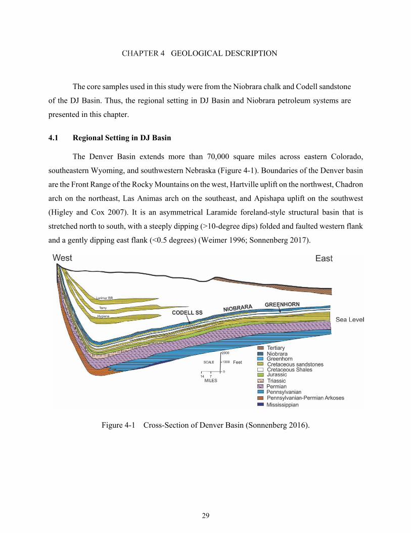
The Denver Basin extends more than 70,000 square miles across eastern Colorado,

southeastern Wyoming, and southwestern Nebraska (Figure 4-1). Boundaries of the Denver basin

are the Front Range of the Rocky Mountains on the west, Hartville uplift on the northwest, Chadron

arch on the northeast, Las Animas arch on the southeast, and Apishapa uplift on the southwest

(Higley and Cox 2007). It is an asymmetrical Laramide foreland-style structural basin that is

stretched north to south, with a steeply dipping (>10-degree dips) folded and faulted western flank

and a gently dipping east flank (<0.5 degrees) (Weimer 1996; Sonnenberg 2017).

 

Figure 4-1 Cross-Section of Denver Basin (Sonnenberg 2016).

30

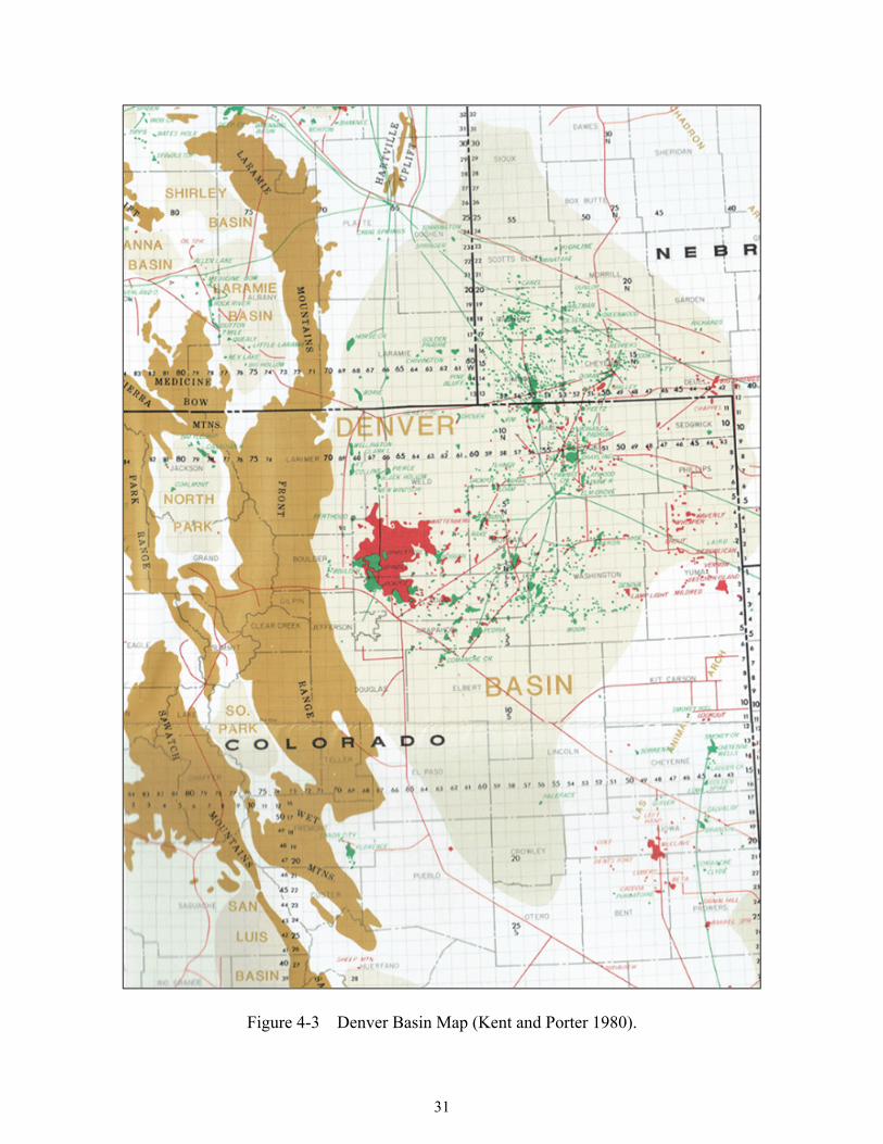
4.2 Niobrara Petroleum System

The Niobrara Formation and Codell sandstone are active plays in the Denver Basin (Figure

4-3). The Codell sandstone occurs between the primary Cretaceous carbonate producing sections,

Niobrara and Greenhorn. Both of these carbonate sections are deep water depositions consisting

of chalks and marls. In between these deep-water depositions, The Codell sandstone is thought to

represent a lowering of sea level between two of the highest sea levels during Cretaceous. The

thickness of Codell averages between 15 to 20 ft in this area. It has a low resistivity due to the clay

and pyrite content. The source rocks for the Codell are the Graneros, Greenhorn, Carlile, and also

the adjacent Niobrara Formation. The source beds are marine Type II (oil prone) kerogen. This

type of source bed can generate both oil and gas (Sonnenberg 2014).

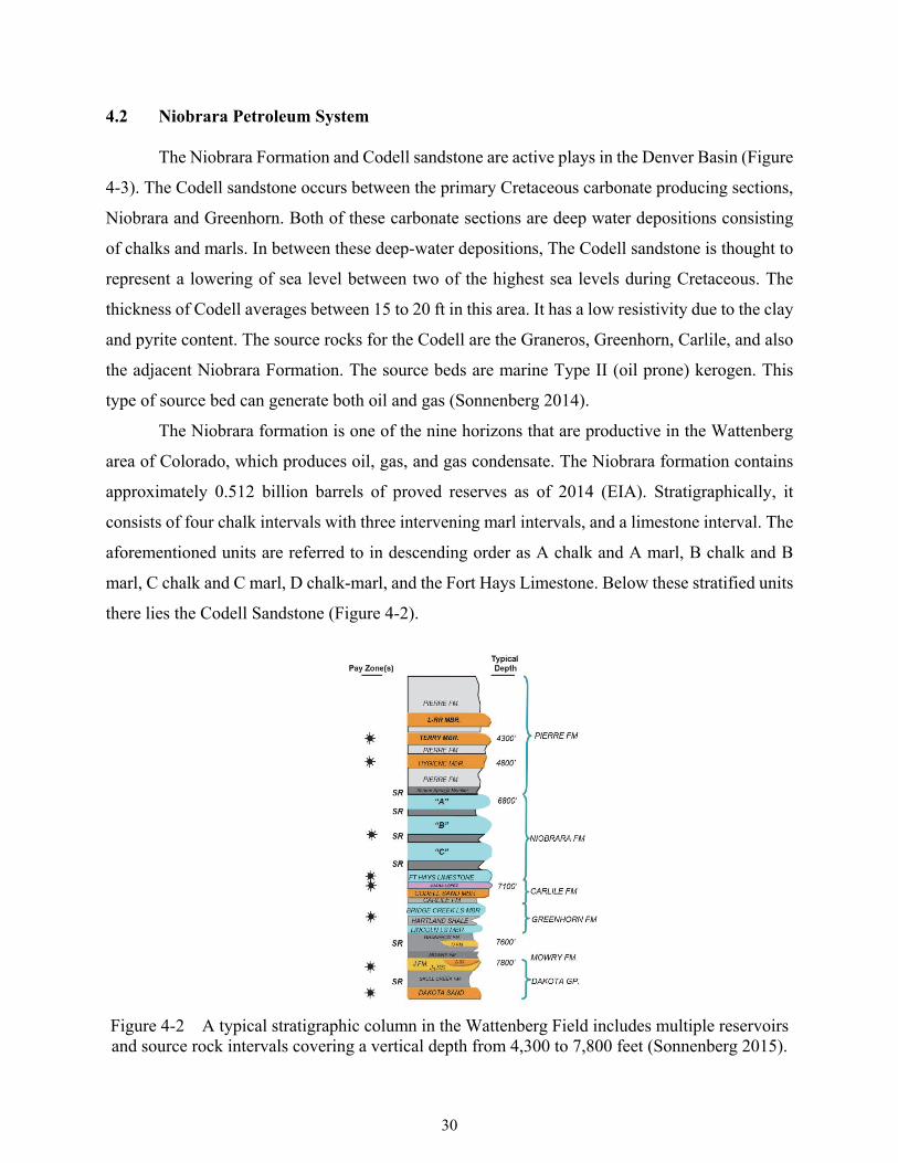
The Niobrara formation is one of the nine horizons that are productive in the Wattenberg

area of Colorado, which produces oil, gas, and gas condensate. The Niobrara formation contains

approximately 0.512 billion barrels of proved reserves as of 2014 (EIA). Stratigraphically, it

consists of four chalk intervals with three intervening marl intervals, and a limestone interval. The

aforementioned units are referred to in descending order as A chalk and A marl, B chalk and B

marl, C chalk and C marl, D chalk-marl, and the Fort Hays Limestone. Below these stratified units

there lies the Codell Sandstone (Figure 4-2).

 Figure 4-2 A typical stratigraphic column in the Wattenberg Field includes multiple reservoirs and source rock intervals covering a vertical depth from 4,300 to 7,800 feet (Sonnenberg 2015).

31

 

Figure 4-3 Denver Basin Map (Kent and Porter 1980).

32

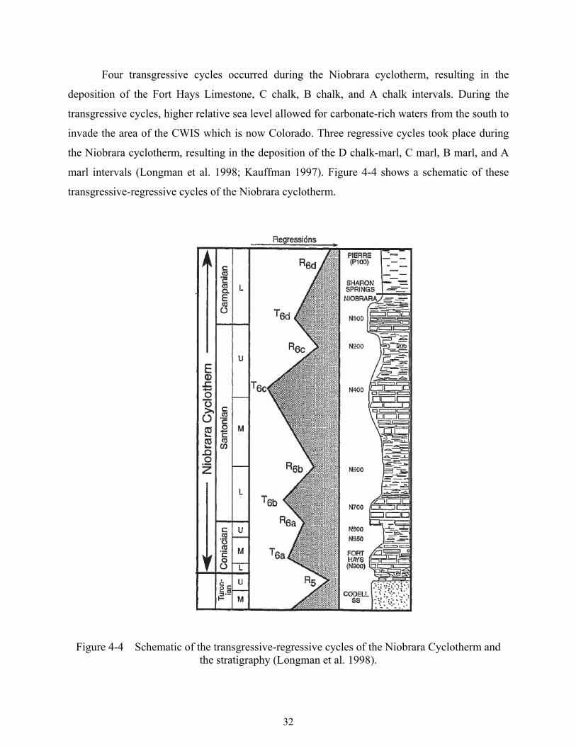
Four transgressive cycles occurred during the Niobrara cyclotherm, resulting in the

deposition of the Fort Hays Limestone, C chalk, B chalk, and A chalk intervals. During the

transgressive cycles, higher relative sea level allowed for carbonate-rich waters from the south to

invade the area of the CWIS which is now Colorado. Three regressive cycles took place during

the Niobrara cyclotherm, resulting in the deposition of the D chalk-marl, C marl, B marl, and A

marl intervals (Longman et al. 1998; Kauffman 1997). Figure 4-4 shows a schematic of these

transgressive-regressive cycles of the Niobrara cyclotherm.

 

  

Figure 4-4 Schematic of the transgressive-regressive cycles of the Niobrara Cyclotherm and the stratigraphy (Longman et al. 1998).

33

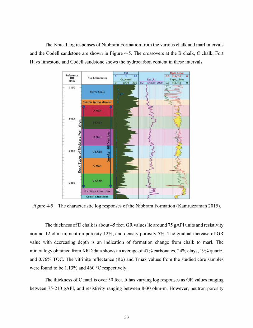
The typical log responses of Niobrara Formation from the various chalk and marl intervals

and the Codell sandstone are shown in Figure 4-5. The crossovers at the B chalk, C chalk, Fort

Hays limestone and Codell sandstone shows the hydrocarbon content in these intervals.

 Figure 4-5 The characteristic log responses of the Niobrara Formation (Kamruzzaman 2015).

 

The thickness of D chalk is about 45 feet. GR values lie around 75 gAPI units and resistivity

around 12 ohm-m, neutron porosity 12%, and density porosity 5%. The gradual increase of GR

value with decreasing depth is an indication of formation change from chalk to marl. The

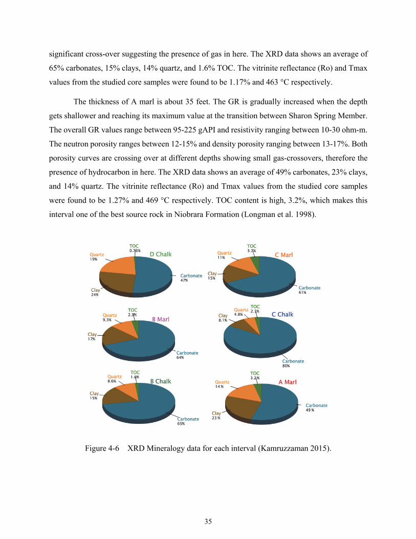
mineralogy obtained from XRD data shows an average of 47% carbonates, 24% clays, 19% quartz,

and 0.76% TOC. The vitrinite reflectance (Ro) and Tmax values from the studied core samples

were found to be 1.13% and 460 °C respectively.

The thickness of C marl is over 50 feet. It has varying log responses as GR values ranging

between 75-210 gAPI, and resistivity ranging between 8-30 ohm-m. However, neutron porosity

34

and density porosity show more or less close values as, 15-25%, and 12-20% respectively and

overlying and crossing each other in different segments suggesting the presence of hydrocarbon

and most probably oil. The varying log response values may be related to transition between chalk

and marl at the edges of the interval. The mineralogy obtained from XRD data shows an average

of 61% carbonates, 15% clays, 11% quartz, and 3.7% TOC. The vitrinite reflectance (Ro) and

Tmax values from the studied core samples were found to be 1.2% and 465 °C respectively. The

high TOC value makes C marl the best hydrocarbon source rock in the Niobrara Formation interval

in the DJ Basin (Longman et al. 1998).

The thickness of C chalk is about 45-50 feet. It has varying log responses as GR values

ranging between 70-200 gAPI but a sharp change from the underlying C marl. The resistivity is

ranging between 25-55 ohm-m. The neutron porosity is showing values of 10-15% and density

porosity values showing values of 12-18% with a significant cross-over suggesting the presence

of gas in here. It has a sharp GR transition from underlying C marl. The XRD data shows an

average of 74% carbonates, 11% clays, 6.8% quartz, and 2.5% TOC. The vitrinite reflectance (Ro)

and Tmax values from the studied core samples were found to be 1.2% and 464 °C respectively.

The thickness of B marl is about 40 feet with parallel-laminated marls with chalky-marl

units. GR response ranges between 125-200 gAPI with a higher GR response near the middle of

the unit, suggesting an increase in shale content. The resistivity is ranging between 12-25 ohm-m

and neutron and density porosity values ranging in between 10-20% and 8-15% respectively. The

values of neutron porosity are higher than the above and below chalk units, showing a divergence

between density porosity and neutron porosity curves suggesting no hydrocarbon content in this

interval. The XRD data shows an average of 62% carbonates, 18% clays, 9.5% quartz, and 2.9%

TOC. The vitrinite reflectance (Ro) and Tmax values from the studied core samples were found to

be 1.25% and 467 °C respectively. Even if the TOC of this unit is lower than the C marl, it still

possesses a good potential to be a source rock.

The thickness of B chalk is about 40 feet interbedded with chalky-marl and marl rock units

(Longman et al. 1998). The GR gradually decreases when the depth gets shallower from the edge

of B marl and ranging between 70-120 gAPI. This interval shows the highest resistivity response

compared to the underlying units where it ranges between 20-200 ohm-m. The neutron porosity is

showing values of 10-12% and density porosity values showing values of 15-19% with a

35

significant cross-over suggesting the presence of gas in here. The XRD data shows an average of

65% carbonates, 15% clays, 14% quartz, and 1.6% TOC. The vitrinite reflectance (Ro) and Tmax

values from the studied core samples were found to be 1.17% and 463 °C respectively.

The thickness of A marl is about 35 feet. The GR is gradually increased when the depth

gets shallower and reaching its maximum value at the transition between Sharon Spring Member.

The overall GR values range between 95-225 gAPI and resistivity ranging between 10-30 ohm-m.

The neutron porosity ranges between 12-15% and density porosity ranging between 13-17%. Both

porosity curves are crossing over at different depths showing small gas-crossovers, therefore the

presence of hydrocarbon in here. The XRD data shows an average of 49% carbonates, 23% clays,

and 14% quartz. The vitrinite reflectance (Ro) and Tmax values from the studied core samples

were found to be 1.27% and 469 °C respectively. TOC content is high, 3.2%, which makes this

interval one of the best source rock in Niobrara Formation (Longman et al. 1998).

Figure 4-6 XRD Mineralogy data for each interval (Kamruzzaman 2015).

36

LABORATORY EXPERIMENTS  

The experiments were conducted in the high-speed centrifuge. 1.5-inch diameter core

plugs were used in this study. This chapter addresses the details of the experimental setup.

This chapter includes (1) core cleaning, (2) equipment used for porosity and

permeability measurement, (3) equipment used for capillary pressure measurement, and (4) the

fluids and the cores used in the experiments.

5.1 Core Cleaning

Core plugs are extracted from core samples as long cylinders of 1-inch or 1.5-inch

diameter. Then, they were cut to appropriate lengths for the needs of further experiments. The

majority of reservoir core samples are either poorly reserved or not preserved at all. To perform

and get accurate results from porosity, permeability, and fluid saturation experiments they need to

be cleaned. The cleaning process is performed to clean the core plug samples from mud filtrates

from the drilling mud, native oil, and connate water.

API RP40 (1998) provides a list of methods for cleaning the core samples:

‐ Solvent Flushing by Direct Pressure

‐ Flushing by centrifuge

‐ Gas driven solvent extraction

‐ Distillation extraction (Soxhlet Extraction)

‐ Liquefied gas extraction

Cores should be cleaned by using at least two solvents of the non-polar and polar-type to

remove all the residual fluids that might affect further parameter measurements and experiment

procedures. Non-polar solvents dissolve the light components of oil whereas polar solvents

dissolve the heavy components of oil along with water and precipitated salts from formation brine.

For cleaning procedures, toluene, xylene, chloroform are the most common non-polar solvents,

and methanol, ethanol, dichloromethane are the most common polar solvents. Usually, a non-polar

solvent is the first to be used to clean the core in the cleaning procedure, which is followed by a

polar solvent.

37

In this research, Soxhlet extractor is chosen as the cleaning method because it is the

cheapest and the quickest method out of the aforementioned methods. Also, several cores can be

placed in the same chamber, and if delicate samples which can be damaged from high pressure or

high temperature can be cleaned by using cool Soxhlet extractor.

Soxhlet extractor can be used to clean a large number of cores depending on the size of the

core samples and the chamber of the apparatus. Firstly, the round bottomed flask which sits on a

heating mantle is filled with the solvent. When the solvent reaches the boiling point, it evaporates.

The evaporated sample travels up to the condenser unit, which is filled with continuously

circulated cold water. The solvent condenses in this unit and drips down to the chamber which

holds the core samples. As the solvent fills the chamber, it submerges the core samples, and it is

soaked through the pore spaces of the samples and dissolves the residual fluids and precipitated

salts. When the level of the solvent reaches the siphon level, the solvent and the dissolved fluids

in the chamber will reflux to the round bottom flask beneath it. Then, the cycle will repeat but

leaving the dissolved fluids in the bottom flask because of the boiling point difference. Therefore,

cores will be exposed to fresh evaporated and condensed solvents each time. Through the cleaning

process, the color change in the bottom flask is checked regularly, and the solvent will be refreshed

or changed if needed.

5.1.1 Cleaning Procedure

All the cores that are used in this study are cleaned with Soxhlet extractor (Figure 5-1).

Solvents that are used are toluene, methanol, and chloroform. Prior to cleaning, all cores that are

selected for cleaning are weighed to see how many residual fluids and precipitated salt be removed.

Firstly, toluene is used to clean the cores. The boiling point of toluene is 110.6°C (Table

5-1). Toluene removes the heavy components of oil, and as it has a high boiling point, it also

removes the residual water (McPhee et al. 2015). However, as toluene has a very high boiling point

and potential to damage the clay minerals as it can also remove the clay-bound water, the hot

toluene extraction kept running only for 2-3 days. The cores kept submerged with toluene in the

chamber for 1-2 weeks more without continuously boiling the solvent but refreshing the solvent

regularly depending on the discoloration. With this method, I try to mimic the effect of cool

Soxhlet extraction. The discoloration occurred every 3-4 hours at the beginning of the cleaning but

the rate decreased after 4-6 days. The decrease on rate was quicker on Niobrara chalk samples

38

compared to Codell sandstone samples. The cores kept in toluene until the discoloration is

minimized. However, the process was stopped after two weeks not to create further damages inside

the core that cannot be seen by the naked eye.

At the end of toluene cleaning stage, core samples will contain precipitated salts because

of the extracted formation water. Also, some of the heavy oil components will be present as well.

Chloroform-methanol azeotrope with 65% and 35% ratio is used for the next stage to complete the

cleaning procedure. An azeotrope is a mixture of two or more solvents. The proportions of the

components are not altered in the distillation process because when boiled, the vapor has the same

proportion as the unboiled mixture. However, this mixture has a significantly lower boiling point

than the individual components. Individually chloroform has a boiling point of 61°C, and methanol

has 64.7°C. However, the azeotrope of chloroform and methanol with a ratio of 65% to 35%, the

boiling point will be decreased to 53.5 °C (Table 5-1). The decrease in the boiling point is also

needed not to damage the clay minerals in the cores. The cores were cleaned with the azeotrope

for a week until the discoloration ceases. It is observed that the cease of discoloration was quicker

on the chalk samples because of their tighter pore structure compared to sandstones. However, the

process stopped after one week of cleaning not to create further damages inside the core that cannot

be seen by naked eye.

Table 5-1 Properties of cleaning solvents (McPhee et al. 2015).

Solvent Boiling Point (°C) Solubility

Toluene 110.6 Oil

Methanol 64.7 Water and salt

Chloroform 61 Oil

Chloroform/Methanol

Azeotrope (65/35)

53.5 Oil, water, and salt

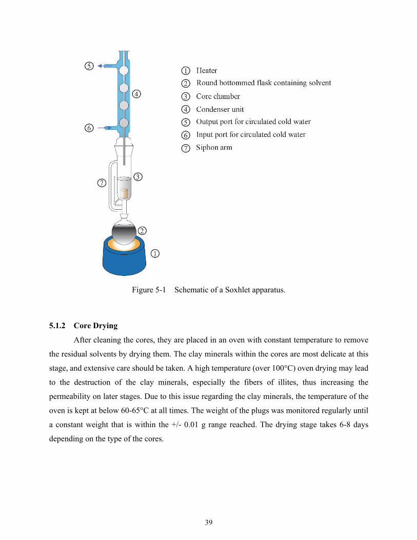
39

 Figure 5-1 Schematic of a Soxhlet apparatus.

5.1.2 Core Drying

After cleaning the cores, they are placed in an oven with constant temperature to remove

the residual solvents by drying them. The clay minerals within the cores are most delicate at this

stage, and extensive care should be taken. A high temperature (over 100°C) oven drying may lead

to the destruction of the clay minerals, especially the fibers of illites, thus increasing the

permeability on later stages. Due to this issue regarding the clay minerals, the temperature of the

oven is kept at below 60-65°C at all times. The weight of the plugs was monitored regularly until

a constant weight that is within the +/- 0.01 g range reached. The drying stage takes 6-8 days

depending on the type of the cores.

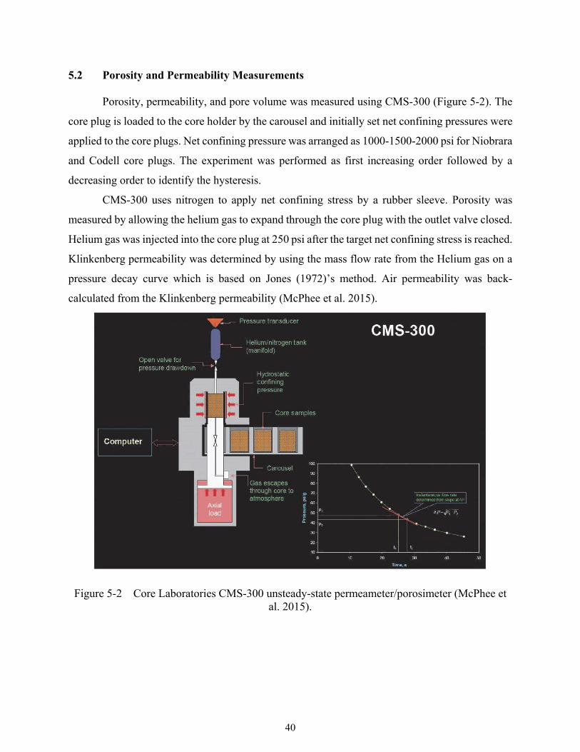
40

5.2 Porosity and Permeability Measurements

Porosity, permeability, and pore volume was measured using CMS-300 (Figure 5-2). The

core plug is loaded to the core holder by the carousel and initially set net confining pressures were

applied to the core plugs. Net confining pressure was arranged as 1000-1500-2000 psi for Niobrara

and Codell core plugs. The experiment was performed as first increasing order followed by a

decreasing order to identify the hysteresis.

CMS-300 uses nitrogen to apply net confining stress by a rubber sleeve. Porosity was

measured by allowing the helium gas to expand through the core plug with the outlet valve closed.

Helium gas was injected into the core plug at 250 psi after the target net confining stress is reached.

Klinkenberg permeability was determined by using the mass flow rate from the Helium gas on a

pressure decay curve which is based on Jones (1972)’s method. Air permeability was back-

calculated from the Klinkenberg permeability (McPhee et al. 2015).

 

Figure 5-2 Core Laboratories CMS-300 unsteady-state permeameter/porosimeter (McPhee et al. 2015).

 

 

41

5.3 Capillary Pressure Concept and Measurements

Capillary pressure is the pressure difference between the adjacent phases of a wetting and

a non-wetting phase at equilibrium. Thus, the capillary pressure can be defined as in Eq. 5-1:

c nw wp p p (5-1)

In a pore space that is occupied with oil and water, as non-wetting and wetting phases

respectively, the fluid saturations are defined as:

1w o

S S (5-2)

The knowledge of capillary effects, which control the distribution of the saturation

gradients of different phases in a pore network, is essential in multi-phase flow through porous

media. The relationship between the capillary pressure and the saturation is vital to understand the

characteristics of the porous medium and how the phases behave when replacing one another. The

relationship between fluid saturation and capillary pressure in a porous medium that is occupied

by oil and water is defined in a sketch in Figure 5-3. In this figure, line 1 represents the drainage

curve, where the non-wetting phase (oil) is displacing the wetting phase (water). The point reaches

maximum capillary pressure, and minimum saturation is irreducible water saturation ,w irrS . Line

2 represents the spontaneous imbibition curve where water is displacing oil without the direction

of the water. Line 3 is forced imbibition where water saturation increases with increasing capillary

pressure until it reaches the residual oil saturation.

There are three main methods currently used in laboratories to determine the capillary

pressure curves; mercury methods, porous plate methods, and centrifuge method. Mercury method

is a quick method that is used to obtain capillary pressure data, pore throat distribution and pore

level heterogeneity. Porous plate method is used to determine the capillary pressure curves and

saturation relationships by using a plate in ambient conditions or confining stress of up to 10,000

psi. The samples that are used for this method should have a permeability above 1 md.

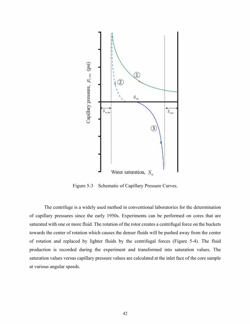
42

 

Figure 5-3 Schematic of Capillary Pressure Curves.

The centrifuge is a widely used method in conventional laboratories for the determination

of capillary pressures since the early 1950s. Experiments can be performed on cores that are

saturated with one or more fluid. The rotation of the rotor creates a centrifugal force on the buckets

towards the center of rotation which causes the denser fluids will be pushed away from the center

of rotation and replaced by lighter fluids by the centrifugal forces (Figure 5-4). The fluid

production is recorded during the experiment and transformed into saturation values. The

saturation values versus capillary pressure values are calculated at the inlet face of the core sample

at various angular speeds.

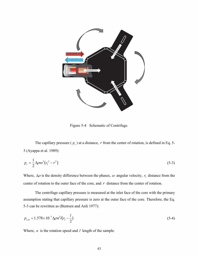
43

Figure 5-4 Schematic of Centrifuge.

The capillary pressure (c

p ) at a distance, r from the center of rotation, is defined in Eq. 5-

3 (Ayappa et al. 1989):

2 2 22

12

( )c

p r r (5-3)

Where, is the density difference between the phases, angular velocity, 2r distance from the

center of rotation to the outer face of the core, and r distance from the center of rotation.

The centrifuge capillary pressure is measured at the inlet face of the core with the primary

assumption stating that capillary pressure is zero at the outer face of the core. Therefore, the Eq.

5-3 can be rewritten as (Bentsen and Anli 1977):

7 221 578 10

2, . ( )c in

lp n l r (5-4)

Where, n is the rotation speed and l length of the sample.

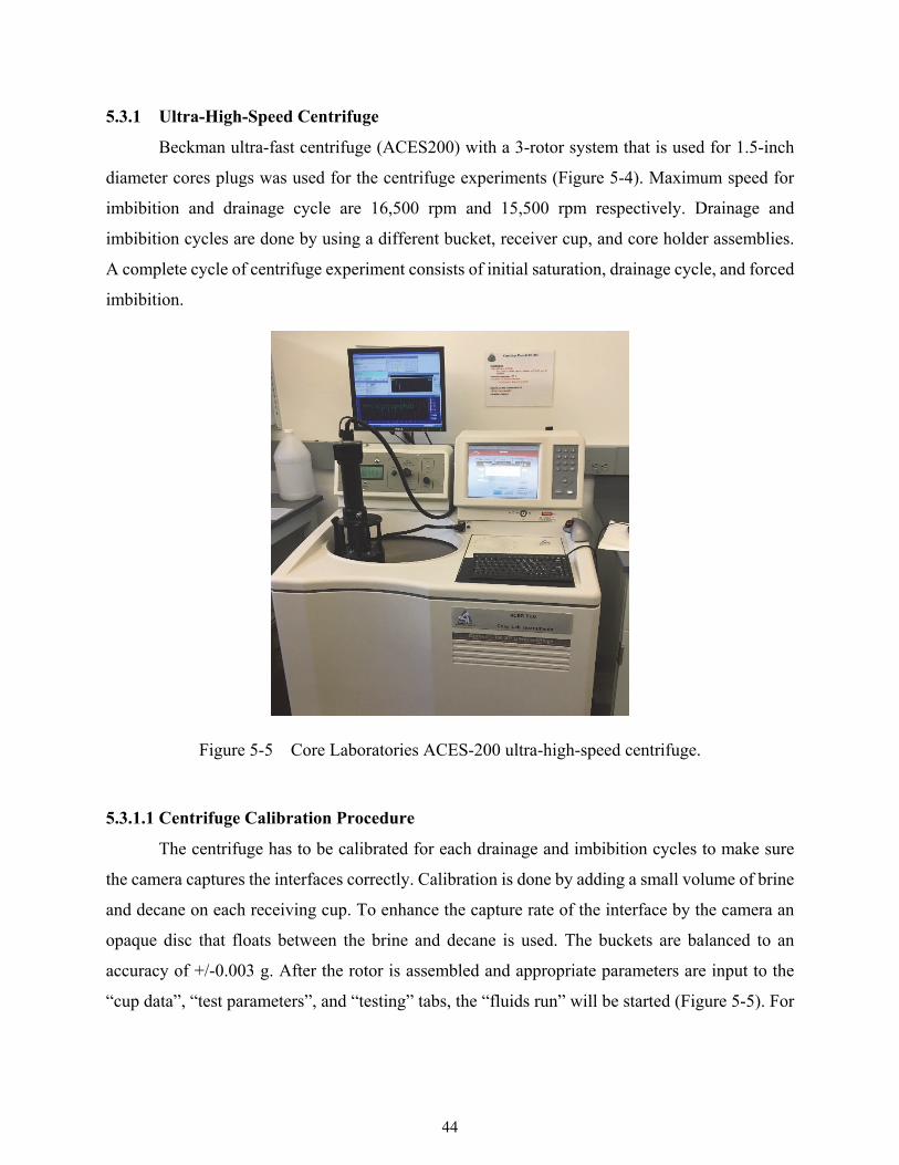
44

5.3.1 Ultra-High-Speed Centrifuge

Beckman ultra-fast centrifuge (ACES200) with a 3-rotor system that is used for 1.5-inch

diameter cores plugs was used for the centrifuge experiments (Figure 5-4). Maximum speed for

imbibition and drainage cycle are 16,500 rpm and 15,500 rpm respectively. Drainage and

imbibition cycles are done by using a different bucket, receiver cup, and core holder assemblies.

A complete cycle of centrifuge experiment consists of initial saturation, drainage cycle, and forced

imbibition.

 

Figure 5-5 Core Laboratories ACES-200 ultra-high-speed centrifuge.

 

5.3.1.1 Centrifuge Calibration Procedure

The centrifuge has to be calibrated for each drainage and imbibition cycles to make sure

the camera captures the interfaces correctly. Calibration is done by adding a small volume of brine

and decane on each receiving cup. To enhance the capture rate of the interface by the camera an

opaque disc that floats between the brine and decane is used. The buckets are balanced to an

accuracy of +/-0.003 g. After the rotor is assembled and appropriate parameters are input to the

“cup data”, “test parameters”, and “testing” tabs, the “fluids run” will be started (Figure 5-5). For

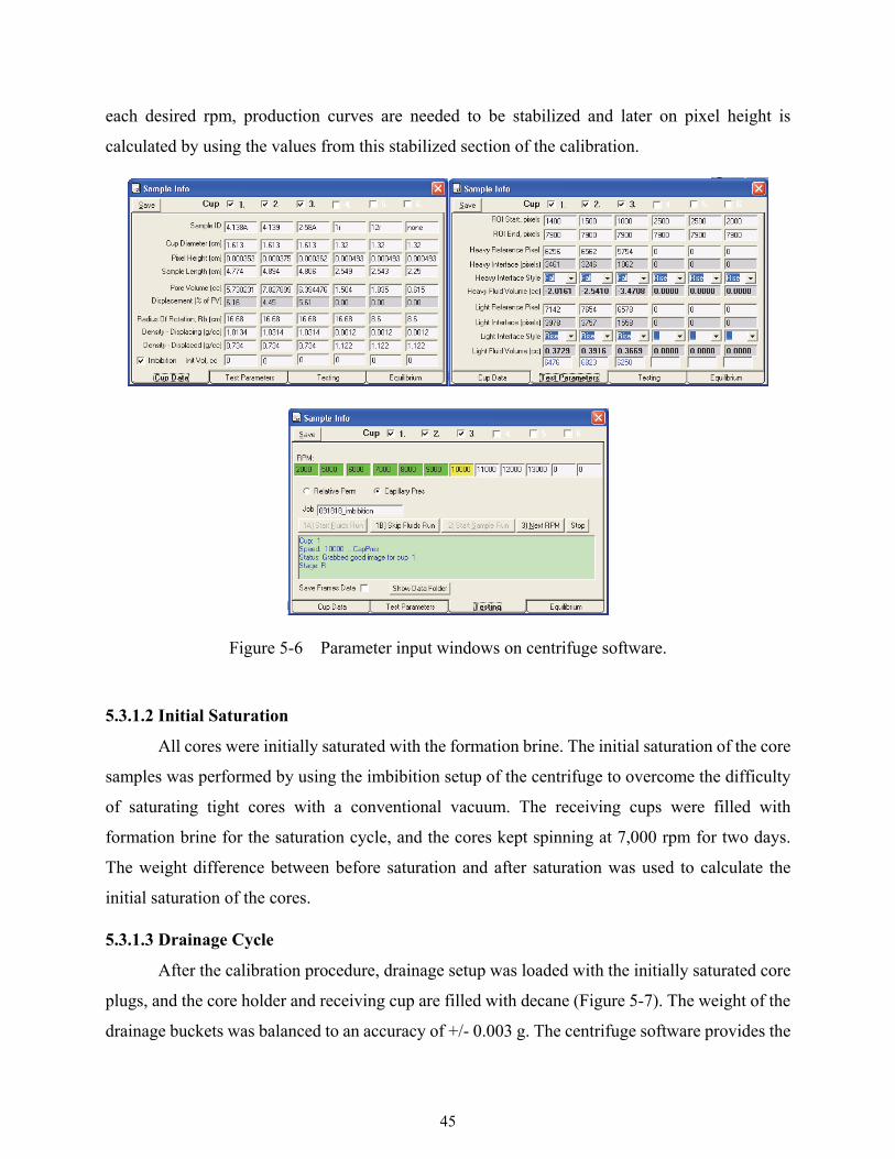
45

each desired rpm, production curves are needed to be stabilized and later on pixel height is

calculated by using the values from this stabilized section of the calibration.

 

Figure 5-6 Parameter input windows on centrifuge software.

 

5.3.1.2 Initial Saturation

All cores were initially saturated with the formation brine. The initial saturation of the core

samples was performed by using the imbibition setup of the centrifuge to overcome the difficulty

of saturating tight cores with a conventional vacuum. The receiving cups were filled with

formation brine for the saturation cycle, and the cores kept spinning at 7,000 rpm for two days.

The weight difference between before saturation and after saturation was used to calculate the

initial saturation of the cores.

5.3.1.3 Drainage Cycle

After the calibration procedure, drainage setup was loaded with the initially saturated core

plugs, and the core holder and receiving cup are filled with decane (Figure 5-7). The weight of the

drainage buckets was balanced to an accuracy of +/- 0.003 g. The centrifuge software provides the

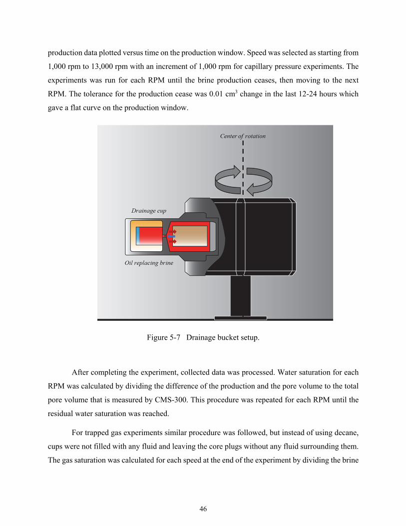
46

production data plotted versus time on the production window. Speed was selected as starting from

1,000 rpm to 13,000 rpm with an increment of 1,000 rpm for capillary pressure experiments. The

experiments was run for each RPM until the brine production ceases, then moving to the next

RPM. The tolerance for the production cease was 0.01 cm3 change in the last 12-24 hours which

gave a flat curve on the production window.

Figure 5-7 Drainage bucket setup.

After completing the experiment, collected data was processed. Water saturation for each

RPM was calculated by dividing the difference of the production and the pore volume to the total

pore volume that is measured by CMS-300. This procedure was repeated for each RPM until the

residual water saturation was reached.

For trapped gas experiments similar procedure was followed, but instead of using decane,

cups were not filled with any fluid and leaving the core plugs without any fluid surrounding them.

The gas saturation was calculated for each speed at the end of the experiment by dividing the brine

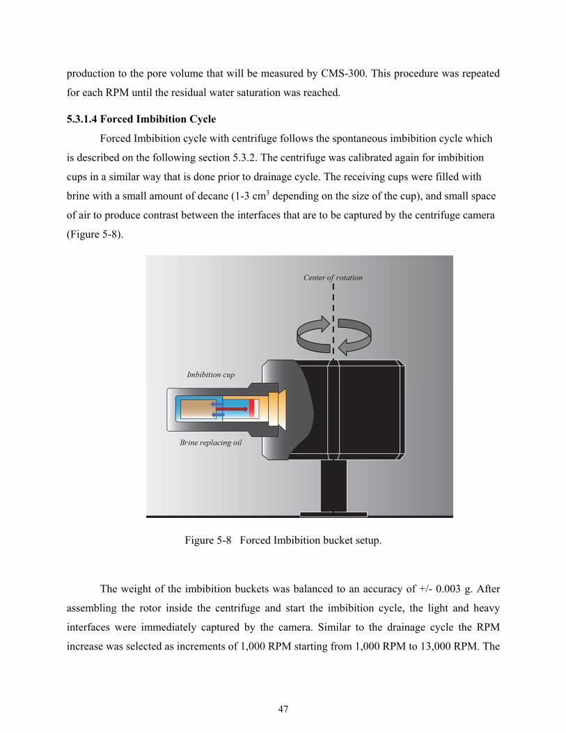
47

production to the pore volume that will be measured by CMS-300. This procedure was repeated

for each RPM until the residual water saturation was reached.

5.3.1.4 Forced Imbibition Cycle

Forced Imbibition cycle with centrifuge follows the spontaneous imbibition cycle which

is described on the following section 5.3.2. The centrifuge was calibrated again for imbibition

cups in a similar way that is done prior to drainage cycle. The receiving cups were filled with

brine with a small amount of decane (1-3 cm3 depending on the size of the cup), and small space

of air to produce contrast between the interfaces that are to be captured by the centrifuge camera

(Figure 5-8).

Figure 5-8 Forced Imbibition bucket setup.

The weight of the imbibition buckets was balanced to an accuracy of +/- 0.003 g. After

assembling the rotor inside the centrifuge and start the imbibition cycle, the light and heavy

interfaces were immediately captured by the camera. Similar to the drainage cycle the RPM

increase was selected as increments of 1,000 RPM starting from 1,000 RPM to 13,000 RPM. The

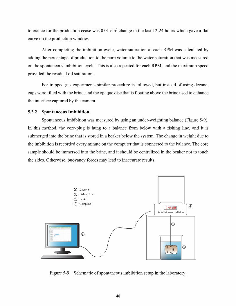
48

tolerance for the production cease was 0.01 cm3 change in the last 12-24 hours which gave a flat

curve on the production window.

After completing the imbibition cycle, water saturation at each RPM was calculated by

adding the percentage of production to the pore volume to the water saturation that was measured

on the spontaneous imbibition cycle. This is also repeated for each RPM, and the maximum speed

provided the residual oil saturation.

For trapped gas experiments similar procedure is followed, but instead of using decane,

cups were filled with the brine, and the opaque disc that is floating above the brine used to enhance

the interface captured by the camera.

5.3.2 Spontaneous Imbibition

Spontaneous Imbibition was measured by using an under-weighting balance (Figure 5-9).

In this method, the core-plug is hung to a balance from below with a fishing line, and it is

submerged into the brine that is stored in a beaker below the system. The change in weight due to

the imbibition is recorded every minute on the computer that is connected to the balance. The core

sample should be immersed into the brine, and it should be centralized in the beaker not to touch

the sides. Otherwise, buoyancy forces may lead to inaccurate results.

 

Figure 5-9 Schematic of spontaneous imbibition setup in the laboratory.

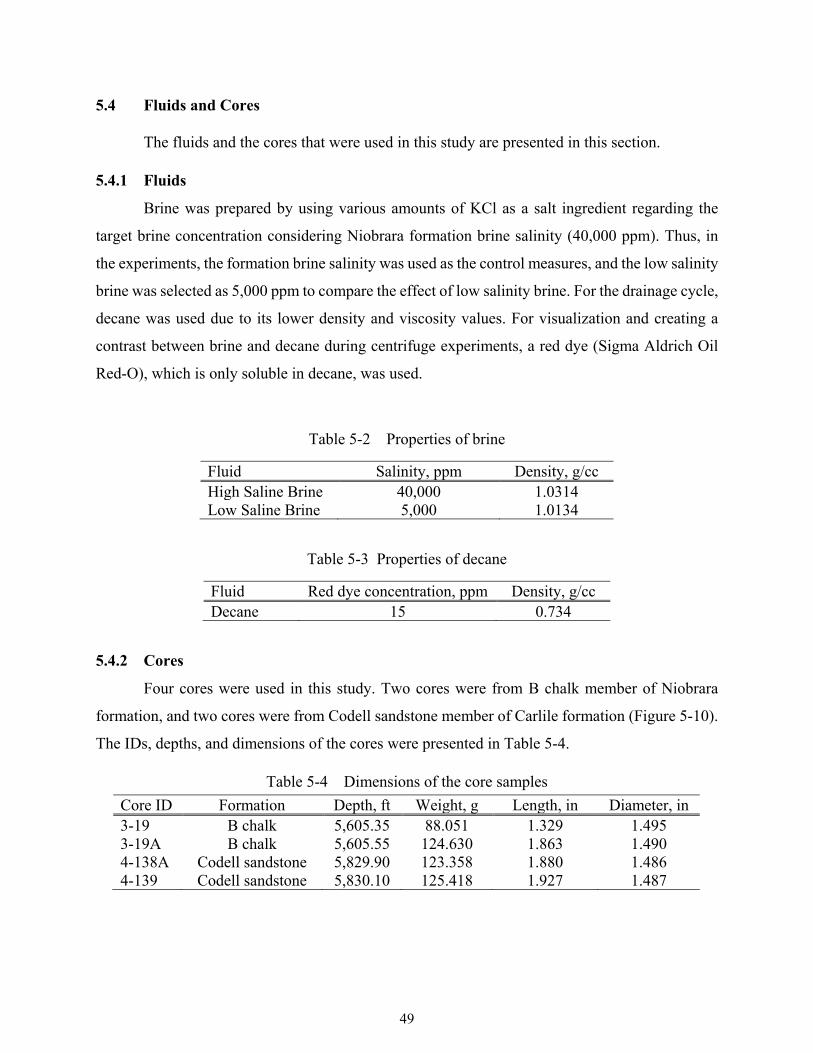
49

5.4 Fluids and Cores

The fluids and the cores that were used in this study are presented in this section.

5.4.1 Fluids

Brine was prepared by using various amounts of KCl as a salt ingredient regarding the

target brine concentration considering Niobrara formation brine salinity (40,000 ppm). Thus, in

the experiments, the formation brine salinity was used as the control measures, and the low salinity

brine was selected as 5,000 ppm to compare the effect of low salinity brine. For the drainage cycle,

decane was used due to its lower density and viscosity values. For visualization and creating a

contrast between brine and decane during centrifuge experiments, a red dye (Sigma Aldrich Oil

Red-O), which is only soluble in decane, was used.

Table 5-2 Properties of brine

Fluid Salinity, ppm Density, g/cc High Saline Brine 40,000 1.0314 Low Saline Brine 5,000 1.0134

 

Table 5-3 Properties of decane

Fluid Red dye concentration, ppm Density, g/cc Decane 15 0.734

 

5.4.2 Cores

Four cores were used in this study. Two cores were from B chalk member of Niobrara

formation, and two cores were from Codell sandstone member of Carlile formation (Figure 5-10).

The IDs, depths, and dimensions of the cores were presented in Table 5-4.

Table 5-4 Dimensions of the core samples

 

Core ID Formation Depth, ft Weight, g Length, in Diameter, in 3-19 B chalk 5,605.35 88.051 1.329 1.495 3-19A B chalk 5,605.55 124.630 1.863 1.490 4-138A Codell sandstone 5,829.90 123.358 1.880 1.486 4-139 Codell sandstone 5,830.10 125.418 1.927 1.487

50

 

Figure 5-10 Cores from Codell formation.

 

 

 

 

 

 

 

 

 

 

 

 

51

TRAPPED GAS

An important topic for gas-condensate reservoirs is quantifying the trapped gas

saturation which cause the gas production to be left behind. When an aquifer is underlying a

gas reservoir, water will imbibe into the gas-saturated zone and traps the gas molecules. This

chapter includes (1) geological overview of Bulo Bulo Field Robore III formation and (2)

description of fluids and cores used in the experiment and results.

6.1 Geological Overview of Bulo Bulo Field Robore III Formation

The cores that are used for trapped gas experiments are from Robore III reservoir in the

Bulo Bulo field, Bolivia. The reservoir formation consists of naturally fractured interbedded shales

and sandstones. The Bulo Bulo field is an anticline located in the Carrasco Province. The reservoir

formation Robore is divided into three as Robore I, II, and III, and Limoncito formation overlies

the Robore I to act as a hydrodynamic seal for the reservoir. According to Navarro (2012) Robore

formation is deposited in a shallow sea platform, and Robore III in particular deposited in a

marginal marine environment dominated by storm waves. The formation is fine to very fine-

grained low porosity sandstones which has quartz as a dominant mineral.

The typical log responses of Robore-III Formation are shown in Figure 6-1, that is logged

from the same well that the core plugs are acquired. Robore III formation is categorized as very-

fine to fine-grained sub-feldspathic sandstones with sharp and subangular clasts. The cement

consists of quartz, feldspar, and calcite. Chlorite and illite are the clay minerals found in the

formation. The dominant pore throat size falls to the range of micropores (less than 0.02-0.06 mm),

but mesopores and macropores are also present.

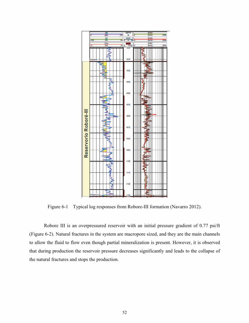
52

 

Figure 6-1 Typical log responses from Robore-III formation (Navarro 2012).

 

Robore III is an overpressured reservoir with an initial pressure gradient of 0.77 psi/ft

(Figure 6-2). Natural fractures in the system are macropore sized, and they are the main channels

to allow the fluid to flow even though partial mineralization is present. However, it is observed

that during production the reservoir pressure decreases significantly and leads to the collapse of

the natural fractures and stops the production.

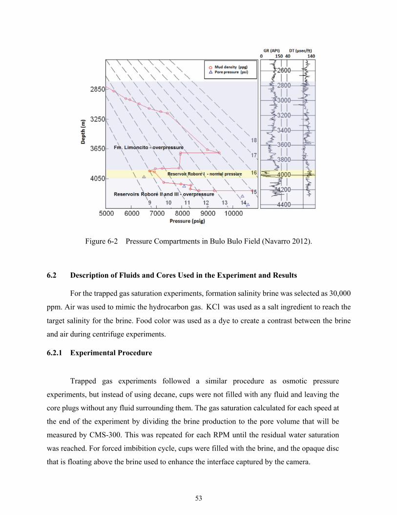
53

 

Figure 6-2 Pressure Compartments in Bulo Bulo Field (Navarro 2012).

 

6.2 Description of Fluids and Cores Used in the Experiment and Results

For the trapped gas saturation experiments, formation salinity brine was selected as 30,000

ppm. Air was used to mimic the hydrocarbon gas. KCl was used as a salt ingredient to reach the

target salinity for the brine. Food color was used as a dye to create a contrast between the brine

and air during centrifuge experiments.

6.2.1 Experimental Procedure  

Trapped gas experiments followed a similar procedure as osmotic pressure

experiments, but instead of using decane, cups were not filled with any fluid and leaving the

core plugs without any fluid surrounding them. The gas saturation calculated for each speed at

the end of the experiment by dividing the brine production to the pore volume that will be

measured by CMS-300. This was repeated for each RPM until the residual water saturation

was reached. For forced imbibition cycle, cups were filled with the brine, and the opaque disc

that is floating above the brine used to enhance the interface captured by the camera.

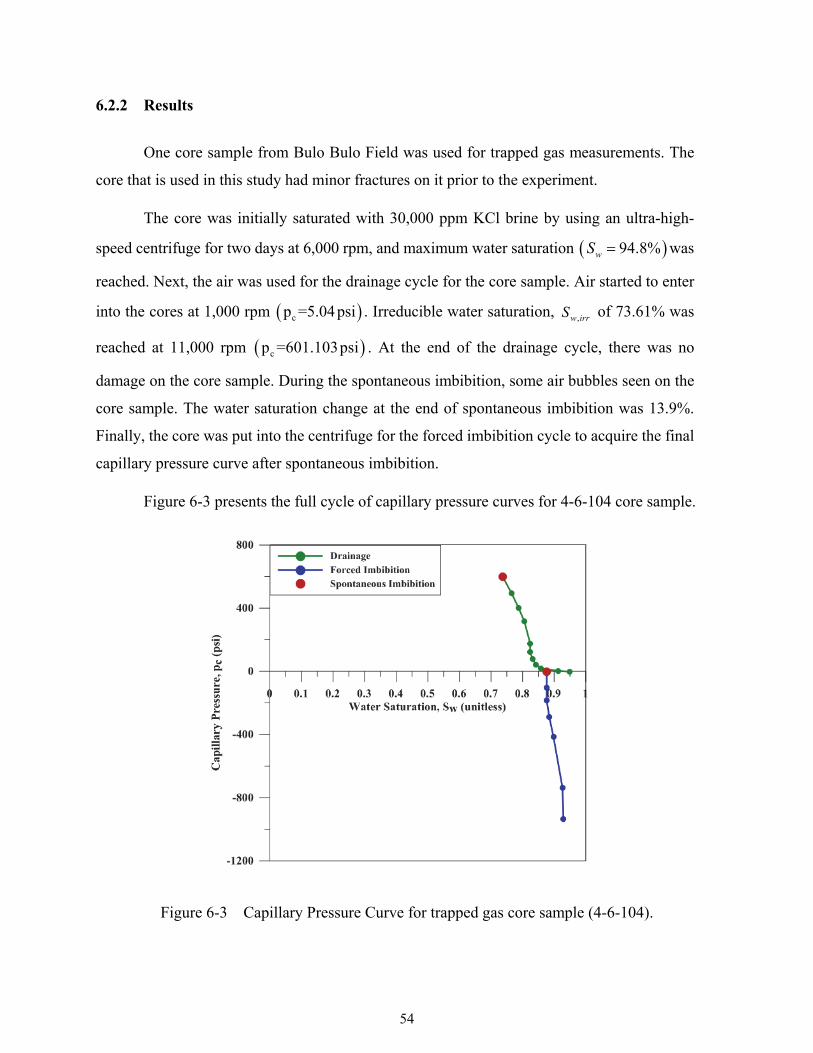
54

6.2.2 Results  

One core sample from Bulo Bulo Field was used for trapped gas measurements. The

core that is used in this study had minor fractures on it prior to the experiment.

The core was initially saturated with 30,000 ppm KCl brine by using an ultra-high-

speed centrifuge for two days at 6,000 rpm, and maximum water saturation 94.8%wS was

reached. Next, the air was used for the drainage cycle for the core sample. Air started to enter

into the cores at 1,000 rpm cp =5.04 psi . Irreducible water saturation, ,w irrS of 73.61% was

reached at 11,000 rpm cp =601.103psi . At the end of the drainage cycle, there was no

damage on the core sample. During the spontaneous imbibition, some air bubbles seen on the

core sample. The water saturation change at the end of spontaneous imbibition was 13.9%.

Finally, the core was put into the centrifuge for the forced imbibition cycle to acquire the final

capillary pressure curve after spontaneous imbibition.

Figure 6-3 presents the full cycle of capillary pressure curves for 4-6-104 core sample.

Figure 6-3 Capillary Pressure Curve for trapped gas core sample (4-6-104).

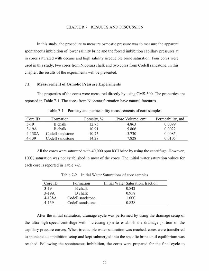
55

RESULTS AND DISCUSSION

 

In this study, the procedure to measure osmostic pressure was to measure the apparent

spontaneous imbibition of lower salinity brine and the forced imbibition capillary pressures at

in cores saturated with decane and high salinity irreducible brine saturation. Four cores were

used in this study, two cores from Niobrara chalk and two cores from Codell sandstone. In this

chapter, the results of the experiments will be presented.

7.1 Measurement of Osmotic Pressure Experiments

The properties of the cores were measured directly by using CMS-300. The properties are

reported in Table 7-1. The cores from Niobrara formation have natural fractures.

Table 7-1 Porosity and permeability measurements of core samples

Core ID Formation Porosity, % Pore Volume, cm3 Permeability, md 3-19 B chalk 12.73 4.863 0.0099 3-19A B chalk 10.91 5.806 0.0022 4-138A Codell sandstone 10.75 5.730 0.0085 4-139 Codell sandstone 14.28 7.828 0.0105

 

All the cores were saturated with 40,000 ppm KCl brine by using the centrifuge. However,

100% saturation was not established in most of the cores. The initial water saturation values for

each core is reported in Table 7-2.

Table 7-2 Initial Water Saturations of core samples

Core ID Formation Initial Water Saturation, fraction 3-19 B chalk 0.842 3-19A B chalk 0.958 4-138A Codell sandstone 1.000 4-139 Codell sandstone 0.838

After the initial saturation, drainage cycle was performed by using the drainage setup of

the ultra-high-speed centrifuge with increasing rpm to establish the drainage portion of the

capillary pressure curves. When irreducible water saturation was reached, cores were transferred

to spontaneous imbibition setup and kept submerged into the specific brine until equilibrium was

reached. Following the spontaneous imbibition, the cores were prepared for the final cycle to

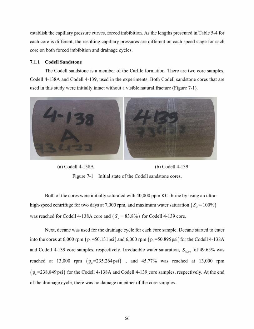
56

establish the capillary pressure curves, forced imbibition. As the lengths presented in Table 5-4 for

each core is different, the resulting capillary pressures are different on each speed stage for each

core on both forced imbibition and drainage cycles.

7.1.1 Codell Sandstone

The Codell sandstone is a member of the Carlile formation. There are two core samples,

Codell 4-138A and Codell 4-139, used in the experiments. Both Codell sandstone cores that are

used in this study were initially intact without a visible natural fracture (Figure 7-1).

(a) Codell 4-138A (b) Codell 4-139 

Figure 7-1 Initial state of the Codell sandstone cores.

Both of the cores were initially saturated with 40,000 ppm KCl brine by using an ultra-

high-speed centrifuge for two days at 7,000 rpm, and maximum water saturation 100%wS

was reached for Codell 4-138A core and 83.8%wS for Codell 4-139 core.

Next, decane was used for the drainage cycle for each core sample. Decane started to enter

into the cores at 6,000 rpm cp =50.131psi and 6,000 rpm cp =50.895psi for the Codell 4-138A

and Codell 4-139 core samples, respectively. Irreducible water saturation, ,w irrS of 49.65% was

reached at 13,000 rpm cp =235.264 psi , and 45.77% was reached at 13,000 rpm

cp =238.849 psi for the Codell 4-138A and Codell 4-139 core samples, respectively. At the end

of the drainage cycle, there was no damage on either of the core samples.

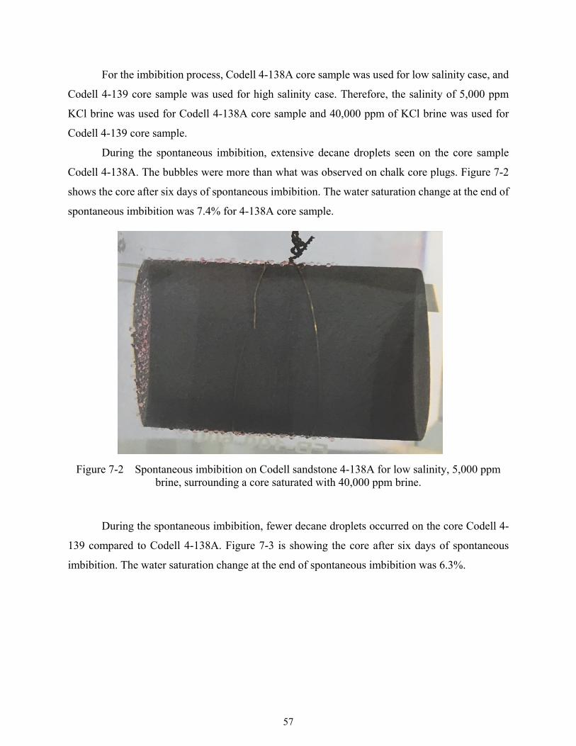
57

For the imbibition process, Codell 4-138A core sample was used for low salinity case, and

Codell 4-139 core sample was used for high salinity case. Therefore, the salinity of 5,000 ppm

KCl brine was used for Codell 4-138A core sample and 40,000 ppm of KCl brine was used for

Codell 4-139 core sample.

During the spontaneous imbibition, extensive decane droplets seen on the core sample

Codell 4-138A. The bubbles were more than what was observed on chalk core plugs. Figure 7-2

shows the core after six days of spontaneous imbibition. The water saturation change at the end of

spontaneous imbibition was 7.4% for 4-138A core sample.

 

Figure 7-2 Spontaneous imbibition on Codell sandstone 4-138A for low salinity, 5,000 ppm brine, surrounding a core saturated with 40,000 ppm brine.

 

During the spontaneous imbibition, fewer decane droplets occurred on the core Codell 4-

139 compared to Codell 4-138A. Figure 7-3 is showing the core after six days of spontaneous

imbibition. The water saturation change at the end of spontaneous imbibition was 6.3%.

58

Figure 7-3 Spontaneous imbibition on Codell sandstone 4-139 for high salinity, 40,000 ppm brine, surrounding a core saturated with 40,000 ppm brine.

Finally, both of the cores put into the centrifuge for the forced imbibition cycle to acquire

the final capillary pressure curve after spontaneous imbibition.

Figure 7-4 presents the full cycle of capillary pressure curves for Codell 4-138A core

sample.

 

Figure 7-4 Capillary Pressure Curve for low salinity core sample (Codell 4-138A).

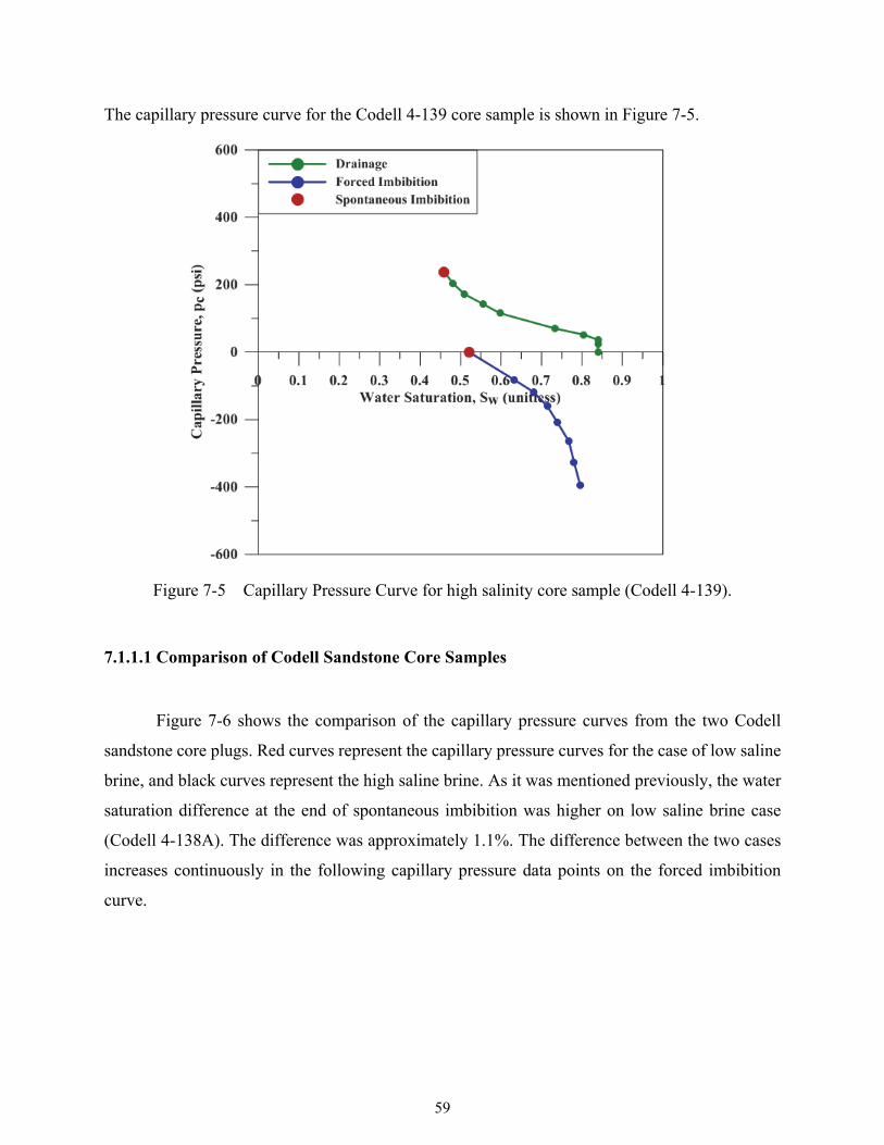
59

The capillary pressure curve for the Codell 4-139 core sample is shown in Figure 7-5.

 

Figure 7-5 Capillary Pressure Curve for high salinity core sample (Codell 4-139).

 

7.1.1.1 Comparison of Codell Sandstone Core Samples

Figure 7-6 shows the comparison of the capillary pressure curves from the two Codell

sandstone core plugs. Red curves represent the capillary pressure curves for the case of low saline

brine, and black curves represent the high saline brine. As it was mentioned previously, the water

saturation difference at the end of spontaneous imbibition was higher on low saline brine case

(Codell 4-138A). The difference was approximately 1.1%. The difference between the two cases

increases continuously in the following capillary pressure data points on the forced imbibition

curve.

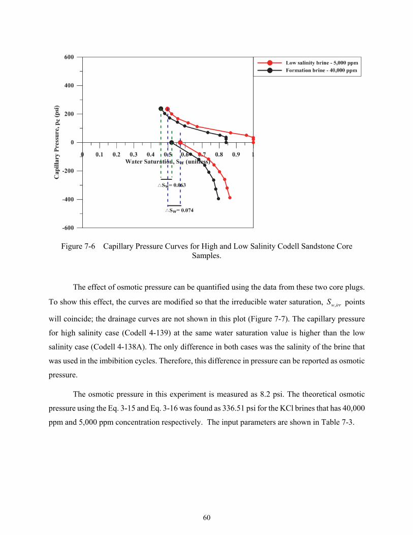
60

 

Figure 7-6 Capillary Pressure Curves for High and Low Salinity Codell Sandstone Core Samples.

The effect of osmotic pressure can be quantified using the data from these two core plugs.

To show this effect, the curves are modified so that the irreducible water saturation, ,w irrS points

will coincide; the drainage curves are not shown in this plot (Figure 7-7). The capillary pressure

for high salinity case (Codell 4-139) at the same water saturation value is higher than the low

salinity case (Codell 4-138A). The only difference in both cases was the salinity of the brine that

was used in the imbibition cycles. Therefore, this difference in pressure can be reported as osmotic

pressure.

The osmotic pressure in this experiment is measured as 8.2 psi. The theoretical osmotic

pressure using the Eq. 3-15 and Eq. 3-16 was found as 336.51 psi for the KCl brines that has 40,000

ppm and 5,000 ppm concentration respectively. The input parameters are shown in Table 7-3.

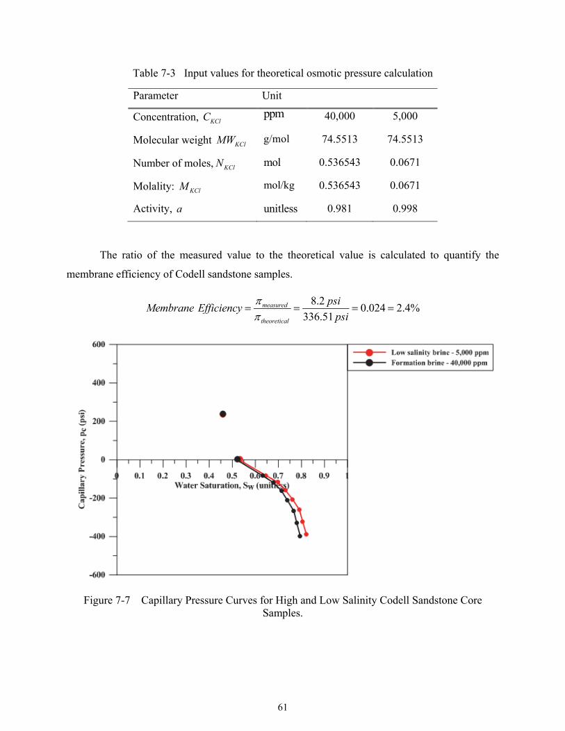
61

Table 7-3 Input values for theoretical osmotic pressure calculation

Parameter Unit

Concentration, KCl

C ppm 40,000 5,000

Molecular weight KCl

MW g/mol 74.5513 74.5513

Number of moles,KCl

N mol 0.536543 0.0671

Molality: KCl

M mol/kg 0.536543 0.0671

Activity, a unitless   0.981 0.998

The ratio of the measured value to the theoretical value is calculated to quantify the

membrane efficiency of Codell sandstone samples.

8.2 0.024 2.4%336.51

measured

theoretical

psiMembrane Efficiency

psi

 

 

Figure 7-7 Capillary Pressure Curves for High and Low Salinity Codell Sandstone Core Samples.

 

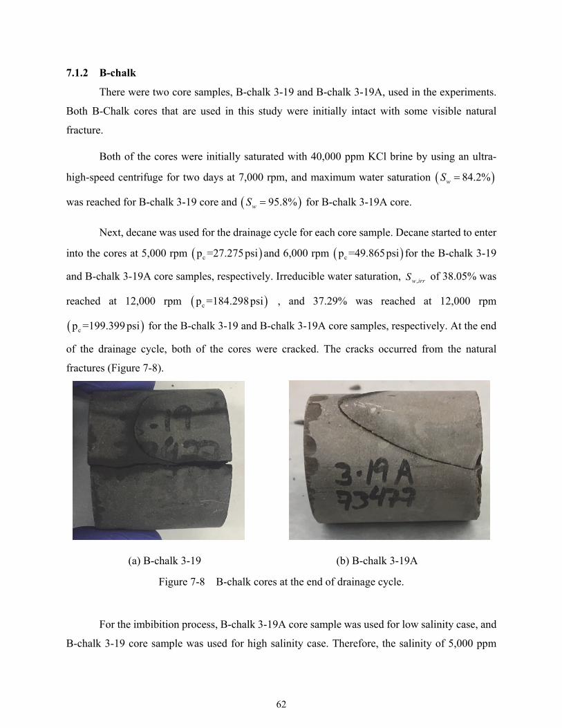
62

7.1.2 B-chalk

There were two core samples, B-chalk 3-19 and B-chalk 3-19A, used in the experiments.

Both B-Chalk cores that are used in this study were initially intact with some visible natural

fracture.

Both of the cores were initially saturated with 40,000 ppm KCl brine by using an ultra-

high-speed centrifuge for two days at 7,000 rpm, and maximum water saturation 84.2%wS

was reached for B-chalk 3-19 core and 95.8%wS for B-chalk 3-19A core.

Next, decane was used for the drainage cycle for each core sample. Decane started to enter

into the cores at 5,000 rpm cp =27.275psi and 6,000 rpm cp =49.865psi for the B-chalk 3-19

and B-chalk 3-19A core samples, respectively. Irreducible water saturation, ,w irrS of 38.05% was

reached at 12,000 rpm cp =184.298psi , and 37.29% was reached at 12,000 rpm

cp =199.399 psi for the B-chalk 3-19 and B-chalk 3-19A core samples, respectively. At the end

of the drainage cycle, both of the cores were cracked. The cracks occurred from the natural

fractures (Figure 7-8).

(a) B-chalk 3-19 (b) B-chalk 3-19A 

Figure 7-8 B-chalk cores at the end of drainage cycle.

 

For the imbibition process, B-chalk 3-19A core sample was used for low salinity case, and

B-chalk 3-19 core sample was used for high salinity case. Therefore, the salinity of 5,000 ppm

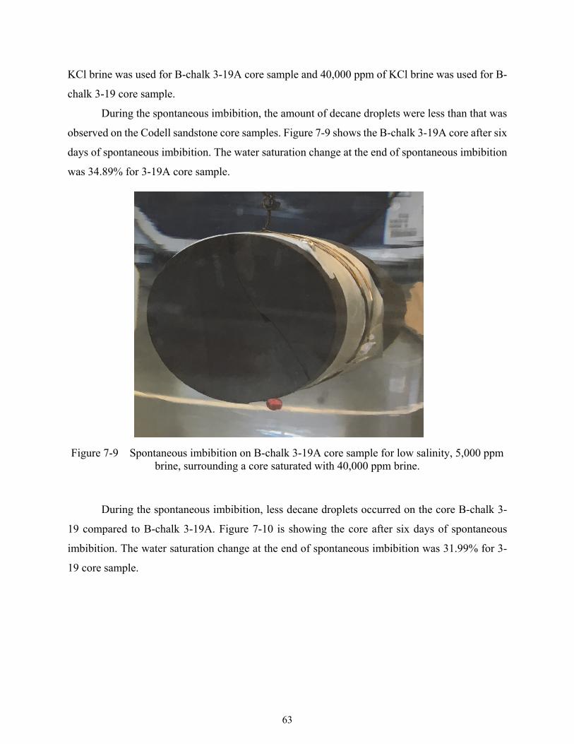
63

KCl brine was used for B-chalk 3-19A core sample and 40,000 ppm of KCl brine was used for B-

chalk 3-19 core sample.

During the spontaneous imbibition, the amount of decane droplets were less than that was

observed on the Codell sandstone core samples. Figure 7-9 shows the B-chalk 3-19A core after six

days of spontaneous imbibition. The water saturation change at the end of spontaneous imbibition

was 34.89% for 3-19A core sample.

 

Figure 7-9 Spontaneous imbibition on B-chalk 3-19A core sample for low salinity, 5,000 ppm brine, surrounding a core saturated with 40,000 ppm brine.

 

During the spontaneous imbibition, less decane droplets occurred on the core B-chalk 3-

19 compared to B-chalk 3-19A. Figure 7-10 is showing the core after six days of spontaneous

imbibition. The water saturation change at the end of spontaneous imbibition was 31.99% for 3-

19 core sample.

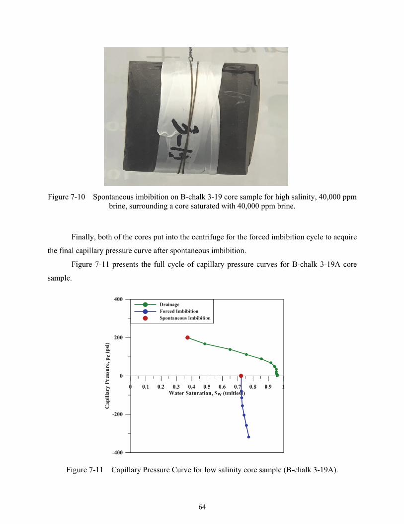
64

Figure 7-10 Spontaneous imbibition on B-chalk 3-19 core sample for high salinity, 40,000 ppm brine, surrounding a core saturated with 40,000 ppm brine.

Finally, both of the cores put into the centrifuge for the forced imbibition cycle to acquire

the final capillary pressure curve after spontaneous imbibition.

Figure 7-11 presents the full cycle of capillary pressure curves for B-chalk 3-19A core

sample.

 

Figure 7-11 Capillary Pressure Curve for low salinity core sample (B-chalk 3-19A).

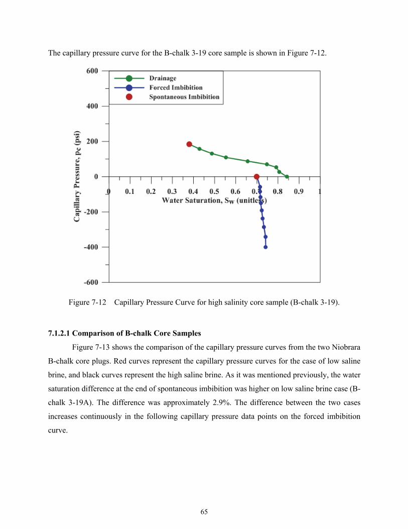
65

The capillary pressure curve for the B-chalk 3-19 core sample is shown in Figure 7-12.

 

Figure 7-12 Capillary Pressure Curve for high salinity core sample (B-chalk 3-19).

 

7.1.2.1 Comparison of B-chalk Core Samples

Figure 7-13 shows the comparison of the capillary pressure curves from the two Niobrara

B-chalk core plugs. Red curves represent the capillary pressure curves for the case of low saline

brine, and black curves represent the high saline brine. As it was mentioned previously, the water

saturation difference at the end of spontaneous imbibition was higher on low saline brine case (B-

chalk 3-19A). The difference was approximately 2.9%. The difference between the two cases

increases continuously in the following capillary pressure data points on the forced imbibition

curve.

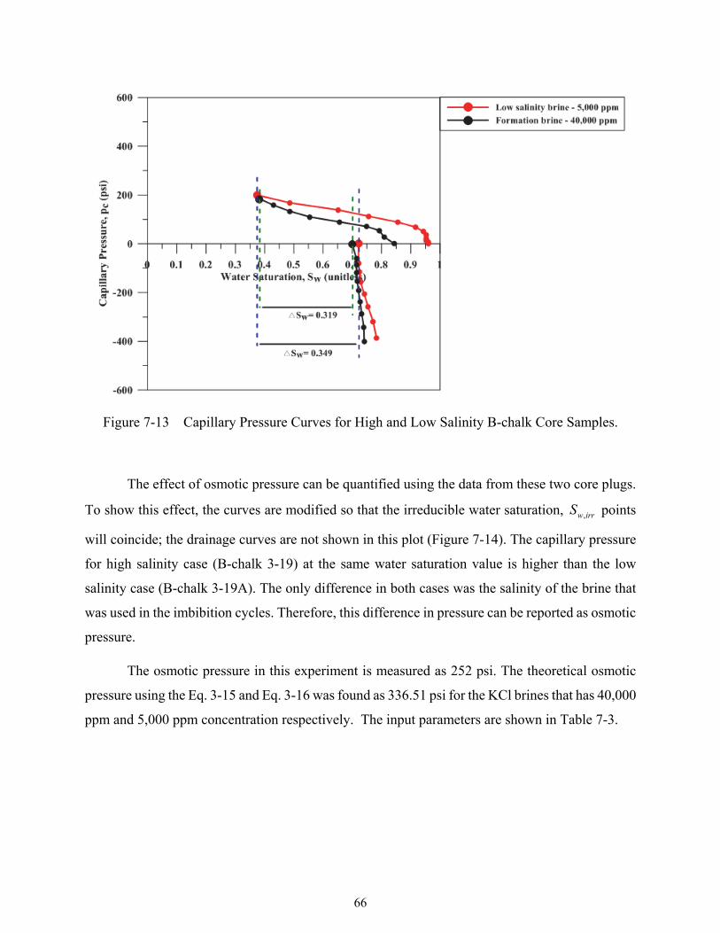
66

 

Figure 7-13 Capillary Pressure Curves for High and Low Salinity B-chalk Core Samples.

The effect of osmotic pressure can be quantified using the data from these two core plugs.

To show this effect, the curves are modified so that the irreducible water saturation, ,w irrS points

will coincide; the drainage curves are not shown in this plot (Figure 7-14). The capillary pressure

for high salinity case (B-chalk 3-19) at the same water saturation value is higher than the low

salinity case (B-chalk 3-19A). The only difference in both cases was the salinity of the brine that

was used in the imbibition cycles. Therefore, this difference in pressure can be reported as osmotic

pressure.

The osmotic pressure in this experiment is measured as 252 psi. The theoretical osmotic

pressure using the Eq. 3-15 and Eq. 3-16 was found as 336.51 psi for the KCl brines that has 40,000

ppm and 5,000 ppm concentration respectively. The input parameters are shown in Table 7-3.

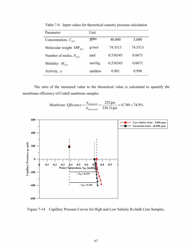
67

Table 7-4 Input values for theoretical osmotic pressure calculation

Parameter Unit

Concentration, KCl

C ppm 40,000 5,000

Molecular weight KCl

MW g/mol 74.5513 74.5513

Number of moles,KCl

N mol 0.536543 0.0671

Molality: KCl

M mol/kg 0.536543 0.0671

Activity, a unitless   0.981 0.998

The ratio of the measured value to the theoretical value is calculated to quantify the

membrane efficiency of Codell sandstone samples.

252psi 0.749 74.9%336.51psi

measured

theoretical

Membrane Efficiency

 

 

Figure 7-14 Capillary Pressure Curves for High and Low Salinity B-chalk Core Samples.

 

68

CONCLUSIONS

In this thesis, the potential for incremental oil recovery for unconventional shale reservoirs

because of the osmotic pressure created via salinity contrast was evaluated. It has been difficult

and time-consuming to measure osmotic pressure in cores. In this thesis, I have introduced a novel

laboratory technique to measure osmotic pressure in very low permeability cores using a high-

speed centrifuge. Specifically, I measure spontaneous and forced imbibition characteristics of

fluids at several salinities in cores saturated with decane at irreducible brine saturation. The

experiments were conducted using Codell sandstone and Niobrara B-chalk core samples. The

40,000 ppm represented the high salinity brine which is the formation brine, and 5,000 ppm

represented the low salinity brine. The following are the main conclusions of this thesis.

Osmotic pressure in a permeable porous material is the external pressure to be applied to

the fluid inside the porous material so that there is no net transfer of solvent across the core

surface. Osmotic pressure is a colligative property meaning that the osmotic pressure is a

function of the molar concentration of the solute particles but not their identity (for

instance, dissolved sodium chloride will be represented at two sets of particles—chlorine

and sodium ions). It should be noted that capillary pressure is dependent on the wettability

of the internal surfaces of pores and the magnitude of the phase saturations in the pores.

On the other hand, osmotic pressure is function of contrast between particle concentrations

outside and inside the pores of the core.

Measured osmotic pressure of Niobrara B-chalk, which has a permeability of 0.0022-

0.0099 md was 74.9 % of the calculated osmotic pressure in a perfect membrane using

activity coefficient. Accounting for chalk solubility in brine within the pores should reduce

the calculated osmotic pressure to about 50% of that in perfect membrane.

Measured osmotic pressure of Codell sandstone, which has a permeability of 0.0085-

0.0105 md was about 2.4 % of the calculated perfect membrane.

 

 

 

69

REFERENCES  

Al-Attar, H.H., Mahmoud, M.Y., and Zekri, A.Y. et al. 2013. Low Salinity Flooding in a Selected Carbonate Reservoir: Experimental Approach. Presented at the EAGE Annual Conference and Exhibition incorporating SPE Europec, London, United Kingdom, 10—13 June. SPE-164788-MS. http://dx.doi.org/10.2118/164788-MS.

Ashraf, A., Hadia, N., and Torsaeter, O. et al. 2010. Laboratory Investigation of Low Salinity Waterflooding as Secondary Recovery Process: Effect of Wettability. Presented at the SPE Oil and Gas India Conference and Exhibition, Mumbai, India, 20—22 January. SPE-129012-MS. http://dx.doi.org/10.2118/129012-MS.

Austad, T., Rezaeidoust, A., and Puntervold, T. 2010. Chemical Mechanism of Low Salinity Water Flooding in Sandstone Reservoirs. Presented at the SPE Improved Oil Recovery Symposium, Tulsa, Oklahoma, 24—28 April. SPE-129767-MS. http://dx.doi.org/10.2118/129767-MS.

Ayappa, K.G., Davis, H.T., and Davis, E.A. et al. 1989. Capillary pressure: Centrifuge method revisited. American Institute of Chemical Engineers 35 (3): 365—372. http://dx.doi.org/10.1002/aic.690350304.

Bentsen, R.G. and Anli, J. 1977. Using Parameter Estimation Techniques To Convert Centrifuge Data Into a Capillary-Pressure Curve. SPE Journal 17 (1). SPE-5026-PA. http://dx.doi.org/10.2118/5026-PA.

Bernard, G.G. 1967. Effect of Floodwater Salinity on Recovery of Oil from Cores Containing Clays. Presented at the SPE California Regional Meeting, Los Angeles, California, 26—27 October. SPE-1725-MS. http://dx.doi.org/10.2118/1725-MS.

BP UK. Clair Ridge, http://www.bp.com/en_gb/united-kingdom/where-we-operate/north-sea/north-sea-major-projects/clair-ridge.html (accessed 28 April 2017).

Callegaro, C., Bartosek, M., and Nobili, M. et al. 2015. Design and Implementation of Low Salinity Waterflood in a North African Brown Field. Presented at the Abu Dhabi International Petroleum Exhibition and Conference, Abu Dhabi, United Arab Emirates, 09—12 November. SPE-177590-MS. http://dx.doi.org/10.2118/177590-MS.

Chapman, D.L. 1913. A contribution to the theory of electrocapillarity. 6, The London, Edinburgh, and Dublin Philosophical Magazine and Journal of Science 25 (148): 475—481.

Dang, C.T.Q., Nguyen, N.T.B., and Chen, Z. 2015. Practical Concerns and Principle Guidelines for Screening, Implementation, Design, and Optimization of Low Salinity Waterflooding. Presented at the SPE Western Regional Meeting, Garden Grove, California, 27—30 January. SPE-174008-MS. http://dx.doi.org/10.2118/174008-MS.

De Sitter, L.U. 1947. Diagenesis of Oil-Field Brines. American Association of Petroleum Geologists Bulletin 31 (11): 2030—2040.

70

Derjaguin, B.V. and Landau, L. 1993. Theory of the stability of strongly charged lyophobic sols and of the adhesion of strongly charged particles in solutions of electrolytes. Progress in Surface Science 43 (1): 30—59. http://dx.doi.org/10.1016/0079-6816(93)90013-L.

Donnan, F.G. 1924. The Theory of Membrane Equilibria. Chemical Reviews 1 (1): 73—90. http://dx.doi.org/10.1021/cr60001a003.

EIA. U.S. Crude Oil and Natural Gas Proved Reserves, Year- end 2016, https://www.eia.gov/naturalgas/crudeoilreserves/pdf/usreserves.pdf (accessed 27 April 2017).

Fakcharoenphol, P., Kurtoglu, B., and Kazemi, H. et al. 2014. The Effect of Osmotic Pressure on Improve Oil Recovery from Fractured Shale Formations. Presented at the SPE Unconventional Resources Conference, The Woodlands, Texas, 01—03 April. SPE-168998-MS. http://dx.doi.org/10.2118/168998-MS.

Farrington, R.A. and Daniels, A. 1979. Phase Equlibria. In Physical Chemistry, fifth edition Chapt. 3, 108—114. New York, New York: John Wiley&Sons.

Gouy, G. 1910. Sur la constitution de la charge electrique a la surface d’un electrolyte, Anniue Physique 9 (4): 457– 468.

Grim, R.E. 1968. Clay Mineral-Organic Reactions. In Clay Mineralogy Chapt. 10, 369—385. New York, New York: McGraw-Hill Book Company.

Hanshaw, B.B. 1962. Membrane properties of compacted clays. Ph.D. dissertation, Harvard University, Cambridge, Massachusetts. 1962.

Hanshaw, B.B. and Coplen, T.B. 1973. Ultrafiltration by a compacted clay membrane—II. Sodium ion exclusion at various ionic strengths. Geochimica et Cosmochimica Acta 37 (10): 2311—2327. http://dx.doi.org/10.1016/0016-7037(73)90106-3.

Hartman, R.J. 1947. Dialysis and Ultrafiltration. In Colloid Chemistry Chapt. 14. London, United Kingdom: The Riverside Press.

Higley, D.K., and Cox, D.O., 2007, Oil and gas exploration and development along the front range in the Denver Basin of Colorado, Nebraska, and Wyoming, in Higley, D.K., compiler, Petroleum systems and assessment of undiscovered oil and gas in the Denver Basin Province, Colorado, Kansas, Nebraska, South Dakota, and Wyoming—USGS Province 39: U.S. Geological Survey Digital Data Series DDS–69–P, ch.2.

Hill, G. A., Colburn, W. A., and Knight J.W., 1961, Reducing oil-finding costs by use of hydrodynamic evaluations. In Evonomics of petroleum exploration, development, and property evaluation. 38-69. Englewood Cliffs, New Jersey: Prentice-Hall

Jadhunandan, P.P. and Morrow, N.R. 1995. Effect of Wettability on Waterflood Recovery for Crude-Oil/Brine/Rock Systems. SPE Reservoir Engineering 10 (1). SPE-22597-PA. http://dx.doi.org/10.2118/22597-PA.

71

Jones, S.C. 1972. A Rapid Accurate Unsteady-State Klinkenberg Permeameter. SPE Journal 12 (5). SPE-3535-PA. http://dx.doi.org/10.2118/3535-PA.

Kamruzzaman, A., 2015. Petrophysical Rock Typing of Unconventional Shale Plays: A Case Study for the Niobrara Formation of the Denver-Julesburg (DJ) Basin. MS Thesis. Colorado School of Mines. Golden, Colorado. 2015.

Kauffman, E.G., 1977, Geological and biological overview: Western Interior Cretaceous basin. The Mountain Geologist, 14(3-4): 75-99.

Kemper, W.D., 1960, Water and ion movement in thin films as influenced by the electrostatic charge and diffuse layers of cations associated with clay mineral surfaces. Soil Sci. Soc. Am. Proc., 24: 10-16.

Kent, H.C. and Porter, K.W. 1980. Colorado Geology. Denver, Colorado: Rocky Mountain Association of Geologists.

Kharaka, Y.K. 1971. Simultaneous flow of water and solutes through geological membranes: experimental and field investigations. Ph.D. dissertation, University of California, Berkeley, California. 1971.

Kharaka, Y. K., and Berry F.A.F., 1973. Simultaneous flow of water and solutes through geological membranes experimental investigation. Geochim. et Cosmochim. Acta. 37: 2577-2603.

Kuznetsov, D., Cotterill, S., and Giddins, M.A. et al. 2015. Low-Salinity Waterflood Simulation: Mechanistic and Phenomenological Models. Presented at the SPE Asia Pacific Enhanced Oil Recovery Conference, Kuala Lumpur, Malaysia, 11—13 August. SPE-174615-MS. http://dx.doi.org/10.2118/174615-MS.

Lager, A., Webb, K.J., and Black, C.J.J. et al. 2008. Low Salinity Oil Recovery - An Experimental Investigation. Petrophysics. 49 (1)

Ligthelm, D.J., Gronsveld, J., and Hofman, J. et al. 2009. Novel Waterflooding Strategy By Manipulation Of Injection Brine Composition. Presented at the EUROPEC/EAGE Conference and Exhibition, Amsterdam, Netherlands, 08—11 June. SPE-119835-MS. http://dx.doi.org/10.2118/119835-MS.

Longman, M.W., Luneau, B. A., and Landon, S. M. 1998, Nature and Distribution of Niobrara Lithologies in the Cretaceous Western Interior of the Rocky Mountain Region. The Mountain Geologist. 35: 137-170.

McGuire, P.L., Chatham, J.R., and Paskvan, F.K. et al. 2005. Low Salinity Oil Recovery: An Exciting New EOR Opportunity for Alaska's North Slope. Presented at the SPE Western Regional Meeting, Irvine, California, 30 March—01 April. SPE-93903-MS. http://dx.doi.org/10.2118/93903-MS.

72

McKelvey, J.G. and Milne, I.H. 1962. The flow of salt solution through compacted clay. Proceedings of the Ninth National Conference on Clays and Clay Minerals: 248—259. http://dx.doi.org/10.1016/B978-1-4831-9842-2.50017-1.

McPhee, C., Reed, J., and Zubizarreta, I. 2015. Routine Core Analysis. In Developments in Petroleum Science Core Analysis: A Best Practice Guide, first edition Chapt. 5, 181—268. Oxford, United Kingdom: Elsevier.

Milne, I.H., McKelvey, J.G., and Trump R.P. 1964. Semi-permeability of bentonite membranes to brines. Bulletin of the American Association of Petroleum Geologists. 48: 103-1O5

Mitchell, J.K. and Soga, K. 2005. Soil Mineralogy. In Fundamentals of Soil Behavior, third edition Chapt. 3. New Jersey: Wiley.

Morrow, N. R. 1990. Wettability and Its Effect on Oil Recovery. Society of Petroleum Engineers. doi:10.2118/21621-PA

Nasralla, R. A., and Nasr-El-Din, H. A. 2011. Impact of Electrical Surface Charges and Cation Exchange on Oil Recovery by Low Salinity Water. Society of Petroleum Engineers. doi:10.2118/147937-MS

Nasralla, R. A., and Nasr-El-Din, H. A. 2014. Double-Layer Expansion: Is It a Primary Mechanism of Improved Oil Recovery by Low-Salinity Waterflooding? Society of Petroleum Engineers. doi:10.2118/154334-PA

Navarro, O.G.V. 2012. Closure of Natural Fractures Caused by Increased Effective Stress, a Case Study: Reservoir Robore III, Bulo Bulo Field, Bolivia . Presented at the SPE Latin America and Caribbean Petroleum Engineering Conference, Mexico City, Mexico, 16—18 April. SPE-153609-MS. http://dx.doi.org/10.2118/153609-MS.

Nguyen, C., Kothamasu, R., He, K., and Xu, L. 2015. Low-Salinity Brine Enhances Oil Production in Liquids-Rich Shale Formations. Society of Petroleum Engineers. http://doi:10.2118/174041-MS

Praustnitz, J.M., Lichtenthaler, R.N., and Azevedo, E.G. 1999. Intermolecular Forces, Corresponding States and Osmotic Systems. In Molecular Thermodynamics of Fluid-phase Equlibria, third edition Chapt. 4. New Jersey: Prentice Hall.

Rivet, S. M., Lake, L. W. and Pope, G. A. 2010. A Core Flooding Investigation of Low Salinity Enhanced Oil Recovery. Paper SPE 134297 presented at the SPE Annual Technical Conference and Exhibition, 19-22 September, Florence, Italy.

Robbana, E., Buikema, T. A., Mair, et al. 2012. Low Salinity Enhanced Oil Recovery - Laboratory to Day One Field Implementation - LoSal EOR into the Clair Ridge Project. Society of Petroleum Engineers. http://doi:10.2118/161750-MS

Sandengen, K. and Arntzen, O.J. 2013. Osmosis During Low Salinity Water Flooding. Presented at the 17th European Symposium on Improved Oil Recovery. Saint Petersburg, Russian Federation, 16—18 April.

73

Sandengen, K., Kristoffersen, A., and Melhuus, K. et al. 2016. Osmosis as Mechanism for Low-Salinity Enhanced Oil Recovery. SPE Journal 21 (4). SPE-179741-PA. http://dx.doi.org/10.2118/179741-PA.

Sheng, J.J. 2014. Critical review of low-salinity waterflooding. Journal of Petroleum Science and Engineering 120: 216—224. http://dx.doi.org/10.1016/j.petrol.2014.05.026.

Sonnenberg, S.A. 2017. Keys to Niobrara and Codell Production, East Pony/Redtail Area, Denver Basin, Colorado. Unconventional Resources Technology Conference.

Sonnenberg, S.A. 2014. The Codell Sandstone Play of the Northern Denver Basin. Unconventional Resources Technology Conference. http://doi:10.15530/URTEC-2014-1917728

Sonnenberg, S.A. 2016. Stratigraphic Architecture of the Niobrara Formation, Wattenberg Field Area, Colorado. Unconventional Resources Technology Conference.

Spagnuolo, M., Callegaro, C., Masserano, F. et al. 2016. Low Salinity Waterflooding: From Single Well Chemical Tracer Test Interpretation to Sector Model Forecast Scenarios. Society of Petroleum Engineers. http://doi:10.2118/179626-MS

Staverman A.J. 1952. Apparent osmotic pressure of solutions of heterodisperse polymers. Recueil des Travaux Chimiques des Pays-Bas 71 Issue 6 623– 633.

Su, J.T., Duncan, P.B., and Mornaya, A. et al. 2010. The effect of hydrogen bonding on the diffusion of water in n-alkanes and n-alcohols measured with a novel single microdroplet method. The Journal of Chemical Physics. http://dx.doi.org/10.1063/1.3298857.

Substech 2017. Stabilization of colloids, http://www.substech.com/dokuwiki/doku.php?id= stabilization_ of_colloids (accessed 28 April 2017)

Takeda, M., Hiratsuka, T., and Ito, K. et al. 2012. Development and Application of a Chemical Osmosis Simulator Based on Tough2. Presented at the TOUGH Symposium, Berkeley, California, 17—19 September.

Tang, G. Q., and Morrow, N. R. 1997. Salinity, Temperature, Oil Composition, and Oil Recovery by Waterflooding. Society of Petroleum Engineers. http://doi:10.2118/36680-PA

Tang, G.Q. and Morrow, N.R. 1999. Influence of brine composition and fines migration on crude oil brine rock interactions and oil recovery. Journal of Petroleum Science&Engineering: 99—111.

Vega Navarro, O. G. 2012. Closure of Natural Fractures Caused by Increased Effective Stress, a Case Study: Reservoir Robore III, Bulo Bulo Field, Bolivia. Society of Petroleum Engineers. http://doi:10.2118/153609-MS

Verbeek P., Matzakos A. 2009. Water Treatment for Flooding with Lower Salinity than Formation Water. Presentation at the Tekna Produced Water Conference, Stavanger, January.

Verwey, E. J. W., and Overbeek, J. Th. G. 1948. Theory of the Stability of Lyophobic Colloids, Elsevier, Amsterdam.

74

Webb, K. J., Black, C. J. J., Al-Ajeel, H. 2004. Low Salinity Oil Recovery - Log-Inject-Log. Paper SPE 89379. SPE/DOE Symposium on Improved Oil Recovery, 17-21 April, Tulsa, Oklahoma, USA.

Webb, K. J., Black, C. J. J., and Tjetland, G. 2005. A Laboratory Study Investigating Methods for Improving Oil Recovery in Carbonates. IPTC 10506. International Petroleum Technology Conference, 21-23 November, Doha, Qatar.

Weimer, R. J., Sonnenberg, S. A., and Young, G. C. 1986, Wattenberg Field, Denver Basin, Colorado, in C. W. Spencer and R. F. Mast, eds., Geology of tight gas reservoirs: Tulsa, Oklahoma, American Association of Petroleum Geologists, p. 143–164.

White, D.E., 1957, Magmatic, connate, and metamorphic waters: Geol. Soc. America Bull. 68 (12): 1659-1682.

Winoto, W., Loahardjo, N., Xie, X. et al. 2012. Secondary and Tertiary Recovery of Crude Oil from Outcrop and Reservoir Rocks by Low Salinity Water Flooding. Paper SPE 154209 presented at the Eighteenth SPE Improved Oil Recovery Symposium, 14-18 April, Tulsa, Oklahoma.

Wood W.W. 1976. A hypothesis of ion filtration in a potable-water aquifer system. Ground WaterI4, 233-244.

Yildiz, H. O., and Morrow, N. R. 1996. Effect of Brine Composition on Recovery of Moutray Crude Oil by Waterflooding. Petroleum Science and Engineering, 14, 159-168.

Yildiz, H. O., Valat, M., and Morrow N. R. 1999. Effect of Brine Composition on Wettability and Oil Recovery of a Prudhoe Bay Crude Oil. Journal of Canadian Petroleum Technology, 38, 1, 26-31.

Yousef, A.A., Al-Saleh, S., and Al-Jawfi, M.S. 2012. The Impact of the Injection Water Chemistry on Oil Recovery from Carbonate Reservoirs. Presented at the SPE EOR Conference at Oil and Gas West Asia, Muscat, Oman, 16—18 April. SPE-154077-MS. http://dx.doi.org/10.2118/154077-MS.

Yousef, A.A., Liu, J.S., and Blanchard, G.W. et al. 2012. Smart Waterflooding: Industry. Presented at the SPE Annual Technical Conference and Exhibition, San Antonio, Texas, 08—10 October. SPE-159526-MS. http://dx.doi.org/10.2118/159526-MS.

Zen, E-An., and Hanshaw, B. B., 1964, Osmotic equilibrium and mechanics of overthrust faulting: Aim. Geol. Soc. America and Assoc. Soc. Joint Mtg. Program, p. 232-233, Miami Beach, Nov. 19-21, 1964; 1965, Geol. Soc. America Spec. Paper 82, p. 232-233.

Zhang, J., Al-Bazali, T. M., Chenevert, M. E. et al. 2008. Factors Controlling the Membrane Efficiency of Shales When Interacting with Water-Based and Oil-Based Muds. Society of Petroleum Engineers.

Zhang, Y. and Sarma, H.K. 2012. Improving Waterflood Recovery Efficiency in Carbonate Reservoirs through Salinity Variations and Ionic Exchanges: A Promising Low-Cost

75

"Smart-Waterflood" Approach. Presented at the Abu Dhabi International Petroleum Conference and Exhibition, Abu Dhabi, United Arab Emirates, 11—14 November. SPE-161631-MS. http://dx.doi.org/10.2118/161631-MS.