DETERMINING THE ACTUAL CANT

GAFIȚOI MARIUS-ANDREI – Assistant Lecturer, Ph.D, Technical University of Civil Engineering of

Bucharest, Faculty of Railways, Roads and Bridges,

e-mail: marius.gafitoi@gmail.com

ANDREI CĂTĂLIN-GHEORGHE – Assistant Lecturer, Ph.D, Technical University of Civil Engineering of

Bucharest, Faculty of Railways, Roads and Bridges,

e-mail: catalinandrei@outlook.com

Abstract: The paper presents the methodology for calculating the actual cant regulated in

Romania and a proposal to improve this methodology. For dealing with the issues regarding

cant determination, actual traffic data was used based on real traffic structure from Chitila-Brazi

section, on the M300/500 Bucharest-Ploiesti.

The proposed methodology for calculating the actual cant is based on a optimization condition

represented by the balancing of the vertical wear for both rails. To accomplish this objective it

was used a weighted average traffic speed, which is unique for a specific traffic structure and

corresponds to all trains.

Keywords: equilibrium speed, uncompensated lateral acceleration, cant deficiency, cant excess,

weighted average traffic speed.

1. Introduction

Adequate design of track geometry is necessary in order to allow the movements of trains to

take place at high speeds and in conditions of maximum safety and comfort. The maximum

traffic speed in a curve is mainly determined by the track geometry: arc curve radius, actual

cant size, type and length of transition spirals.

In track geometry design the cant has the most important role in determining traffic speeds in

curves. The problems that cause rail wear across curves are known [1] but the multitude of

particularities and parameters that appear in the calculation of an accurate cant can do this

task extremely difficult [2].

First of all, this paper presents the methodology for calculating the cant according to the

Railway administration in Romania [3]. Secondly, it presents the proposed methodology for

establishing actual cant according to the weighted average traffic speed of all trains. In order

to illustrate the calculation of actual cant on curves from lines with mixed traffic, a particular

traffic section was chosen. Real traffic structure data was extracted from section Chitila -

Brazi, on the M300/500 Bucharest – Ploiesti.

2. Actual curve cant

Cant is noted with „h” and it is traditionally known as the difference in level between the

inner rail and outer rail. Cant is considered positive when the outer rail on a curved track is

raised above the inner rail and it is considered negative when the inner rail on a curved track

is raised above the outer rail. The cant applicable to a single isolated curve for all trains in

circulation is called actual cant. This is calculated so the following requirements are ensured:

the same life cycle cost of the two rails; comfort conditions (limiting lateral accelerations) and

vehicle stability.

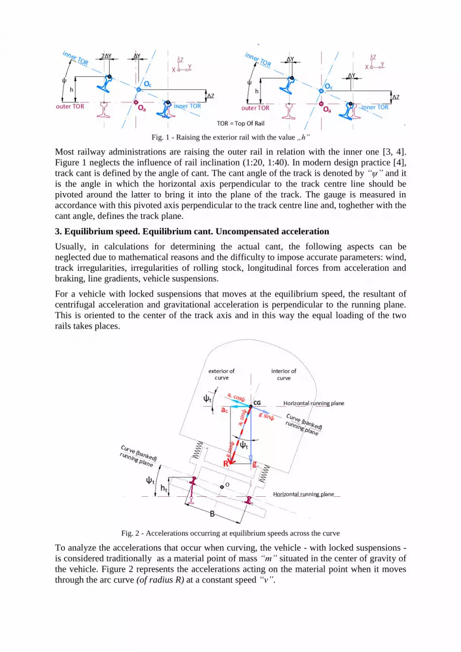
Fig. 1 - Raising the exterior rail with the value „h”

Most railway administrations are raising the outer rail in relation with the inner one [3, 4].

Figure 1 neglects the influence of rail inclination (1:20, 1:40). In modern design practice [4],

track cant is defined by the angle of cant. The cant angle of the track is denoted by “ψ” and it

is the angle in which the horizontal axis perpendicular to the track centre line should be

pivoted around the latter to bring it into the plane of the track. The gauge is measured in

accordance with this pivoted axis perpendicular to the track centre line and, toghether with the

cant angle, defines the track plane.

3. Equilibrium speed. Equilibrium cant. Uncompensated acceleration

Usually, in calculations for determining the actual cant, the following aspects can be

neglected due to mathematical reasons and the difficulty to impose accurate parameters: wind,

track irregularities, irregularities of rolling stock, longitudinal forces from acceleration and

braking, line gradients, vehicle suspensions.

For a vehicle with locked suspensions that moves at the equilibrium speed, the resultant of

centrifugal acceleration and gravitational acceleration is perpendicular to the running plane.

This is oriented to the center of the track axis and in this way the equal loading of the two

rails takes places.

Fig. 2 - Accelerations occurring at equilibrium speeds across the curve

To analyze the accelerations that occur when curving, the vehicle - with locked suspensions -

is considered traditionally as a material point of mass “m” situated in the center of gravity of

the vehicle. Figure 2 represents the accelerations acting on the material point when it moves

through the arc curve (of radius R) at a constant speed “v”.

The uncompensated acceleration aq parallel to the running plane is resulting from below

equations. For an angle value “ψ”, appropriate for an equilibrium speed (ψ = ψt), the

resultant acceleration parallel to the running plane is zero. For the given set of parameters the

equilibrium cant is establish as below:

2

2

2 20

2

03,6

      11,8   

1.500 1

9,81

q c tq

z c

z

c tt

a a cos gsin hVa g

Ba a sin gcos R

a gv Va hR R

B mmcos

mhgsin

B s

(1)

Equilibrium speed is given by the following formula:

20 0          0.293

11,8

tt

h RV V Rh

(2)

At the equilibrium speed both rails (inner and outer) are equally loaded, i.e. they have the

same vertical wear (UV) on the running surface. As not all trains have the same speed when

crossing the same curve, it can be said that equilibrium cant would correspond to a virtual

medium speed.

In reality, the vehicle is fitted with suspensions that act as a separation between suspended

mass and suspension unsprung mass. The existence of suspensions provokes the tilting of the

coach body relative to the running plane. It is considered that the vehicle's center of gravity

has a certain height from the rolling plane and the suspensions show stiffness.

When curving, the vehicle platform tilts towards the outside of the curve with an angle “ψC”

relative to the horizontal plane. This angle is called quasi-static roll angle: 𝜓𝐶 < 𝜓.

The quasi-static lateral acceleration ai (at track level, but parallel to the vehicle floor) is a

measure of the acceleration felt by passengers inside the vehicle. Below equation shows the

compensation effect of the lateral acceleration through curve cant. It also shows the

unfavorable effect of increasing the ai acceleration because of the tilting motion made by

vehicle body. For a non-tilting train ai is greater than the lateral non-compensated acceleration

in the track plane „aq” [4].

1i qa s a (3)

If the suspension stiffness is smaller, then the roll flexibility coefficient “s” is higher. It is

limited to s = 0,4, to ensure the power supply from the overhead contact line [3].

Accelerations for unsprung mass and suspended mass are different because of the suspension:

𝑎𝑞 < 𝑎𝑖.

4. Cant deficiency and cant excess

The difference between the equilibrium cant “ht”, corresponding to a given speed “V”, and

the actual cant „hef” is called actual cant deficiency “Ief” and it is determined by the

following formula:

2

  11,8ef t ef efV

I h h hR

(4)

Cant deficiency occurs only if the speed of the vehicle is above the equilibrium speed.

Between the uncompensated acceleration “aq” and actual cant deficiency “Ief” exists the

following link:

2

12,96  1500 153

ef efq q

gh IVa a

R

(5)

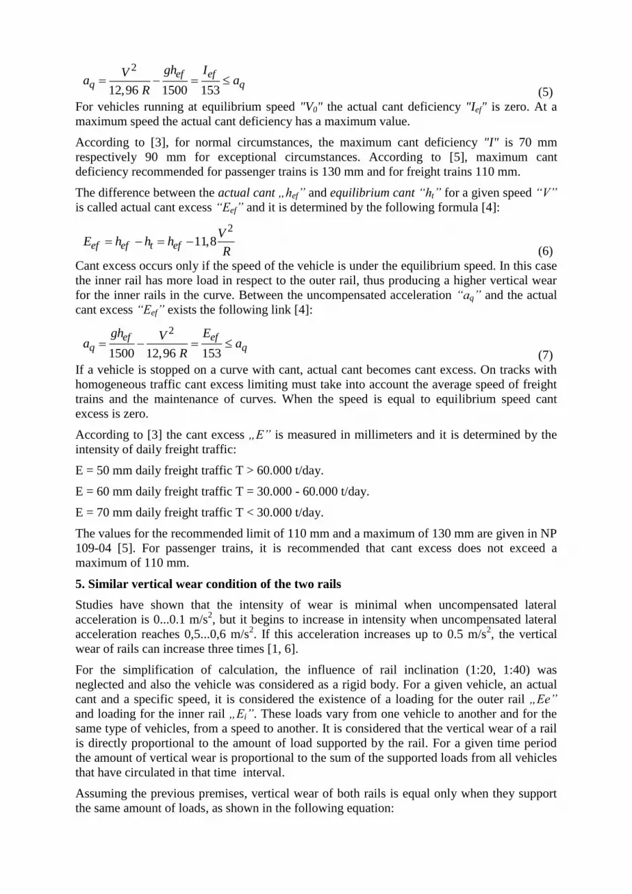
For vehicles running at equilibrium speed "V0" the actual cant deficiency "Ief" is zero. At a

maximum speed the actual cant deficiency has a maximum value.

According to [3], for normal circumstances, the maximum cant deficiency "I" is 70 mm

respectively 90 mm for exceptional circumstances. According to [5], maximum cant

deficiency recommended for passenger trains is 130 mm and for freight trains 110 mm.

The difference between the actual cant „hef” and equilibrium cant “ht” for a given speed “V”

is called actual cant excess “Eef” and it is determined by the following formula [4]:

2

  11,8ef ef t efV

E h h hR

(6)

Cant excess occurs only if the speed of the vehicle is under the equilibrium speed. In this case

the inner rail has more load in respect to the outer rail, thus producing a higher vertical wear

for the inner rails in the curve. Between the uncompensated acceleration “aq” and the actual

cant excess “Eef” exists the following link [4]:

2

1500 12,96  153

ef efq q

gh EVa a

R

(7)

If a vehicle is stopped on a curve with cant, actual cant becomes cant excess. On tracks with

homogeneous traffic cant excess limiting must take into account the average speed of freight

trains and the maintenance of curves. When the speed is equal to equilibrium speed cant

excess is zero.

According to [3] the cant excess „E” is measured in millimeters and it is determined by the

intensity of daily freight traffic:

E = 50 mm daily freight traffic T > 60.000 t/day.

E = 60 mm daily freight traffic T = 30.000 - 60.000 t/day.

E = 70 mm daily freight traffic T < 30.000 t/day.

The values for the recommended limit of 110 mm and a maximum of 130 mm are given in NP

109-04 [5]. For passenger trains, it is recommended that cant excess does not exceed a

maximum of 110 mm.

5. Similar vertical wear condition of the two rails

Studies have shown that the intensity of wear is minimal when uncompensated lateral

acceleration is 0...0.1 m/s2, but it begins to increase in intensity when uncompensated lateral

acceleration reaches 0,5...0,6 m/s2. If this acceleration increases up to 0.5 m/s

2, the vertical

wear of rails can increase three times [1, 6].

For the simplification of calculation, the influence of rail inclination (1:20, 1:40) was

neglected and also the vehicle was considered as a rigid body. For a given vehicle, an actual

cant and a specific speed, it is considered the existence of a loading for the outer rail „Ee”

and loading for the inner rail „Ei”. These loads vary from one vehicle to another and for the

same type of vehicles, from a speed to another. It is considered that the vertical wear of a rail

is directly proportional to the amount of load supported by the rail. For a given time period

the amount of vertical wear is proportional to the sum of the supported loads from all vehicles

that have circulated in that time interval.

Assuming the previous premises, vertical wear of both rails is equal only when they support

the same amount of loads, as shown in the following equation:

e ii iE E (8)

Considering the fact that the track is the same for all trains running within a 24 hours interval,

and considering that all wagons from a train are of the same type, the following conclusions

arise:

2

ie i i ii

v hE E n Q

gR B

(9)

Since cant "h" is the same for all vehicles:

2i i i

i i

n Q vBh

gR n Q

(10)

The weighted average traffic speed is calculated as follows:

2 2 2 221 1 1 1 2 2 2 3 3 3

. .1 1 2 2 3 3

1

       

mi i ii

med tonaj med tonajmi ii

n Q V n Q V n Q V n Q VV V

n Q n Q n Qn Q

(11)

6. Establishing the cant domain

Every curve from an alignment must have its own cant domain defined. It is defined as the set

from which it can be chosen an actual cant appropriate to design parameters considered for an

initial track geometry design. Cant domain refers to the following:

- compliance with maximum cant deficiency "I" where passenger trains running at top

speed „Vmax”;

- compliance with maximum cant excess "E" for freight trains running at minimum

speed „Vmin”;

- compliance with upper limit for the actual cant of 150 mm;

- compliance with the lower limit for the actual cant of 15 mm.

Cant related to specific speeds is calculated with the following formulas:

2 2

11,8 153 11,8max maxn q

V Vh a I

R R

(12) 2 2

11,8 153 11,8min minmax q

V Vh a E

R R

(13)

Every cant domain has a specific minimum design radius corresponding to the design

parameters:

2 211,8 max min

MM

EV IVR

h I E

(14)

Where the value chosen for „hM” is calculated:

2

2 2

2 2 2

1

min

max max minM

max minmin

max

VE I

V EV IVh

V VV

V

(15)

If the calculated value exceeds the maximum allowed limit, the appropriate value from

Regulation no. 314 must be chosen, and for Romanian railways this is 150 mm [3].

The cant domain of actual cant can be a graphical analysis within the system of axes [2].

Where the abscissa shows the curvatures K=1/R (the reciprocal of the radii of curvature) and

the ordinate shows the values of system cant h.

From the points representing the values of cant deficiency and cant excess are starting points

for the lines IVmax and EVmin. These two lines are calculated with the equation (12)

respectively (13). Actual cant domain is the polygon highlighted in figures 3 and 4. Choosing

the actual cant should be based on an optimization condition.

Fig. 3 – The determination of actual cant domain when M is under „hmax”

Fig. 4 – The determination of actual cant domain when M is above „hmax”

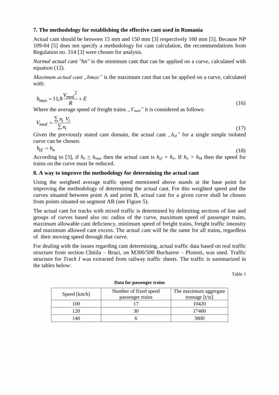
7. The methodology for establishing the effective cant used in Romania

Actual cant should be between 15 mm and 150 mm [3] respectively 160 mm [5]. Because NP

109-04 [5] does not specify a methodology for cant calculation, the recommendations from

Regulation no. 314 [3] were chosen for analysis.

Normal actual cant "hn" is the minimum cant that can be applied on a curve, calculated with

equation (12).

Maximum actual cant „hmax” is the maximum cant that can be applied on a curve, calculated

with:

2

11,8 medmax

Vh E

R

(16)

Where the average speed of freight trains „Vmed” it is considered as follows:

 i imed

i

n VV

n

(17)

Given the previously stated cant domain, the actual cant „hef” for a single simple isolated

curve can be chosen:

ef nh h (18)

According to [3], if hn ≤ hmax then the actual cant is hef = hn. If hn > hM then the speed for

trains on the curve must be reduced.

8. A way to improve the methodology for determining the actual cant

Using the weighted average traffic speed mentioned above stands at the base point for

improving the methodology of determining the actual cant. For this weighted speed and the

curves situated between point A and point B, actual cant for a given curve shall be chosen

from points situated on segment AB (see Figure 5).

The actual cant for tracks with mixed traffic is determined by delimiting sections of line and

groups of curves based also on: radius of the curve, maximum speed of passenger trains,

maximum allowable cant deficiency, minimum speed of freight trains, freight traffic intensity

and maximum allowed cant excess. The actual cant will be the same for all trains, regardless

of their moving speed through that curve.

For dealing with the issues regarding cant determining, actual traffic data based on real traffic

structure from section Chitila – Brazi, on M300/500 Bucharest – Ploiesti, was used. Traffic

structure for Track I was extracted from railway traffic sheets. The traffic is summarized in

the tables below:

Table 1

Data for passenger trains

Speed [km/h] Number of fixed speed

passenger trains

The maximum aggregate

tonnage [t/zi]

100 17 10420

120 30 17400

140 6 3800

Table 2

Data for freight trains

Speed [km/h] Number of fixed speed

passenger trains

The maximum aggregate

tonnage [t/zi]

50 1 700

60 1 2000

70 25 56000

80 32 58670

Table 3

Data for curve radius

Curve number Radius [m] hef [mm]

1 1.800 60

2 1.500 100

3 2.150 50

4 1.980 60

5 1.500 100

6 1.856 80

Knowing the traffic structure and using equation (11), a weighted average traffic speed was

calculated. It is equal to 85,45 km/h. The following weighted equilibrium cant „htp” is

corresponding to this above speed:

2.

11,8med tonaj

tp

Vh

R

(19)

For a maximum speed of 140 km/h and a minimum speed of freight trains of 50 km/h, the

cant domain is according to figure 5.

Using the parameters from Regulation no. 314 [3] it was chosen a maximum cant deficiency

of 70 mm and an cant excess of up to 50 mm due to more than 60.000 tons/day freight traffic.

Fig. 5 – Cant domain for 140/50 km/h speeds

From the traffic structure and the choice of cant domain defined by the maximum and

minimum speed of trains it can be obtained the following: minimum design radius for the rail

traffic structure trafficking, curves radius for which can be applied weighted equilibrium cant

„htp”, curves radius which can be applied Normal actual cant "hn". Curve radius and cant at

point B, for which htp = hn, is calculated with the following equations:

2 2

11,8 max minB

V VR

I

(20) 2

2 2min

B

max min

IVh

V V

(21)

The table below shows the curves which have the actual cant chosen from the cant domain

found in figure 5:

Table 4

Actual cant in respect to radius

Radius [m] Actual cant [mm] Segment from cant

domain

> 5684 15 A-min

5684 - 2086 htp (19) AB

2086 - 1682 hn (12) BM

For curves with a radius less than 1682 m it is necessary to introduce speed limit. For the

analyzed rail sector the following actual cant table resulted:

Table 5

Actual cant for section Chitila – Brazi, on M300/500 Bucharest - Ploiesti

Radius

[m] Actual cant [mm] hn [mm]

htp

[mm]

Segment from

cant domain

1800 58 58 47 BM

1850 55 55 46 BM

1980 47 47 43 BM

2160 39 37 39 AB

9. Conclusions

Because the high-speed lines are only dedicated to one specific type of traffic, the task of the

permanent way designer is simpler. Instead, for mixed traffic lines, it is required to specify the

actual traffic structure and to predict the evolution of traffic for the future so that the

permanent way designer can choose the right design parameters and establish a correct

minimum design radius.

The main disadvantage in determining the actual cant according to the traffic structure is

represented by the high volume of calculations and traffic interpretation.

The methodology for determining the actual cant from Regulation no. 314 may be improved

by introducing in the calculation process the minimum traffic speed instead of the medium

traffic speed. Also the most important aspect could be the introduction of the optimization

condition that ensures similar vertical wear of the inner and outer rails.

By entering into calculations the optimization condition, it is proposed that, if possible, actual

cant to be considered equal to the equilibrium cant corresponding to the weighted average

traffic speed.

References

1. Jin, X.S., et al., An investigation into the effect of train curving on wear and contact stresses of wheel

and rail. Tribology International, 2009. 42(3): p. 475-490.

2. Radu, C., Determinarea supraînălțării efective în curbele de cale ferată, 2000, UTCB - CFDP:

București.

3. CFR, Instrucția de norme și toleranțe pentru construcția și întreținerea căii, Linii cu ecartament

normal, nr. 314, 1989.

4. SR 13803-1: Aplicaţii feroviare. Cale. Parametrii de proiectare ai traseului căii. Ecartament 1435 mm

şi mai mare. Partea 1: Linie obişnuită, 2010.

5. CFR, NP 109-04: Normativ privind proiectarea liniilor și stațiilor de cale ferată pentru viteze până la

200 km/h., 2004.

6. Gailiene, I., Investigation into the calculation of superelevation defects on conventional rail lines.

Transport, 2012. 27(3): p. 229-236.

Symbol used:

v - velocity of the vehicle in a curve [m/s];

V - velocity of the vehicle in a curve [km/h];

V0 - equilibrium speed [km/h];

g - gravitational acceleration [m/s2];

R - radius of studied horizontal curve [m];

B - distance between wheel treads of an axle (on track with gauge1435 mm: B=1500 mm);

ht - equilibrium cant [mm];

ac - centripetal acceleration [m/s2];

aq - non-compensated lateral acceleration in the running plane [m/s2];

az - acceleration in the perpendicular direction [m/s2].

ai - quasi-static lateral acceleration, at track level, but parallel to the vehicle floor [m/s2];

s - the roll flexibility coefficient.

Ee - amount of loading by the outer curve rail;

Ei - amount of loading by the inner curve rail.

ni - number of trains with speed vi;

Qi - tonnage of trains with speed vi.