MARINE ECOLOGY PROGRESS SERIESMar Ecol Prog Ser

Vol. 220: 59–72, 2001 Published September 27

INTRODUCTION

Understanding the horizontal and vertical scales ofvariability of phytoplankton in the ocean is a necessarystep in interpreting the food available to herbivores,and understanding the environment through whichthey must navigate for food. Numerous studies haveconcluded that crustaceans and fish larvae were food-limited at the values of chlorophyll or carbon measuredin situ (e.g., review in Owen 1989, Tiselius 1992, Saizet al. 1993, Cowles & Fessenden 1995). Many herbi-vores have been shown to respond to micropatchinessin the laboratory (e.g., Bird & Kitting 1982, Tiselius1992, Saiz et al. 1993) and in mesocosms (e.g., Bohrer1980, Price 1989), and micropatches of food may benecessary to the foraging success of many marineinvertebrates and vertebrates.

The exploration of microscale (<1 m) structure ofplankton in the oceans has been a technology-limitedenterprise. Owen (1989) discussed how the advent ofthe O-ring facilitated the development of in situ pro-filing fluorometers. The first continuous profiles ofphytoplankton fluorescence with microscale resolution(Derenbach et al. 1979) showed strong variability onvertical scales of 10s of cm. These thin features wereinterpreted as layers which might have formed bydeceleration of sinking phytoplankton at micropycno-clines. The next major advance came with the devel-opment of the laser fluorometer (Cowles et al. 1993,Desiderio et al. 1993), capable of measuring in situfluorescence emission spectra with centimeter-scalevertical resolution. Again, profiles made with thisinstrument showed variability at ~10 cm scales. Thesethin features were interpreted as being thin layers ofphytoplankton, of unknown horizontal extent. A 3-foldincrease in fluorescence over 10 to 20 cm was not un-usual in these profiles, confirming similar results ob-

© Inter-Research 2001

*E-mail: pfranks@ucsd.edu

Microscale distributions of phytoplankton:initial results from a two-dimensional imaging

fluorometer, OSST

Peter J. S. Franks*, Jules S. Jaffe

Scripps Institution of Oceanography, University of California San Diego, 9500 Gilman Drive, La Jolla, California 92093-0218, USA

ABSTRACT: A digital camera system was designed to photograph laser-stimulated fluorescence ofphytoplankton in situ at 0.67 × 0.67 cm resolution over an area of 70 × 70 cm. In a series of verticalprofiles, 1200 images were collected. Criteria were developed to reject images smeared by cameramotions (due to ship heave), and images taken when vertical velocities were >0.2 m s–1, leaving 240good images. Horizontal velocities calculated using ancillary data from the FishTV imaging sonarshowed the water to be directed toward the imaging plane during the deployment, supporting thehypothesis that images were uncontaminated by mixing from the instrument package. Images pass-ing all the criteria show strong isotropic spatial variability. The averaged spatial spectrum was flat,suggesting an underlying random distribution of brightly fluorescent particles—probably phyto-plankton aggregates. Such observations have important implications for our understanding of thefood environment of herbivorous zooplankton, and the mechanisms creating and maintaining patch-iness in the ocean.

KEY WORDS: Microscale · Patchiness · Fluorescence · Phytoplankton · Fluorometer

Resale or republication not permitted without written consent of the publisher

Mar Ecol Prog Ser 220: 59–72, 2001

tained with high-resolution series of bottle samples(Owen 1989, Bjornsen & Nielsson 1991, Tiselius etal. 1994). Owen (1989), however, interpreted his thinlayers as being only about 4 times greater in horizon-tal extent than vertical, but still not isotropic. Franks(1995) presented a mechanism for the formation ofthin layers of phytoplankton through the interactionof existing horizontal patchiness and internal-wave-generated vertical shear. Based on reasonable shearsand the thickness of observed layers, Franks inferredhorizontal scales of <100 m for 30 cm thick layers, or~1 km horizontal scales for layers 2 m thick.

Here we present results from the first deployment ofa novel in situ fluorescence imaging system, the Opti-cal Serial Section Tomography (OSST) system. Thissystem uses a vertical sheet of laser light to inducefluorescence, which is recorded by a sensitive CCD(charge coupled device) camera. In contrast to othersystems, OSST allows the observation of fluorescenceemission in a 2-dimensional plane. The system achieved0.67 cm resolution over an area of 70 × 70 cm. Giventhat this paper describes a new instrument, much ofthe material in the ‘Methods’ section is related to theinstrument’s operation, selection and analysis of theimages, and supporting analyses. Readers not inter-ested in the technical aspects of the system are invitedto skip to the ‘Results and discussion’.

METHODS

OSST. The OSST uses an argon-ion laser to stimulatefluorescence in a vertical (x,z) sheet of illumination(Fig. 1). This fluorescence is photographed with a sen-sitive 1024 × 1024 CCD camera (Photometrics, Tuscon,AZ, USA) fixed 1 m away from the 2 to 3 mm thick lasersheet. All laser wavelengths below 520 nm were usedto excite fluorescence, and a long-pass (>680 nm) filterwas used on the camera. The camera’s field of viewwas 70 cm × 70 cm, and images were binned 10 × 10 toimprove the signal-to-noise ratio and increase the re-fresh rate. Each element of the 102 × 102 image had aresolution of 0.67 cm × 0.67 cm. The camera’s depth offield was made very small (3 cm) to defocus out-of-plane light at wavelengths >680 nm (both fluorescedand scattered). Although this out-of-focus light willcontribute to background levels, it will not contributeto observed spatial structures (but see the subsection‘OSST impulse and frequency response’, below).

Images were corrected for non-uniform illuminationusing an internal calibration: the intensity of light atthe camera is proportional to the intensity of incidentillumination and the concentration of fluorescent mate-rial (see Palowitch & Jaffe 1994, 1995, for a more com-plete derivation):

(1)

where Ii (x,z;r2) is the intensity of light in the (x,z) planerecorded by the camera system a distance r1 from thesource and a distance r2 from the camera, Is(x,z;r2) isthe intensity of the stimulating wavelength λ s at a point(x,z) in the viewed field, and λe is the emission wave-length; the concentration of the fluorescing compoundis C(x,z;r2). Fluorescence intensity is reduced by ineffi-ciencies in the fluorescing processes, spherical spread-ing of light, and camera limitations, all represented byκ. The first integral term accounts for attenuation of thestimulating beam along its path r1 from the source tothe point (x,z). The second integral represents absorp-tion of fluoresced light along its path r2 from (x,z) to thecamera. An additive factor of the camera’s dark cur-rent, Idc, must also be considered:

Iobs(x,z;r2) = Ii (x,z;r2) + Idc (2)

The raw data must be processed to produce an imagein which the intensity of any pixel is proportional to theamount of fluorescing material there (assumed here tobe chlorophyll a). We estimated the in-plane concentra-

I x z r I x z r C x z r

rC r r

rC r r

i

r r

( , ; ) ( , ; ) ( , ; )

exp ( , ) exp ( , )

2 2 2

12 1 1

22 2 2

1 1

1 2

=

−

−

∫ ∫

κ

λ λ

s

s ed d

60

b

cd

e

a

z

x

y

Fig. 1. Schematic of the OSST system showing camera hous-ing (a), imaged area in the laser sheet (b), spar holding thefiber optic lens forming the laser sheet (c), FishTV (d), vanedirecting the system into the current (e), and coordinate axis.The hydro wire was connected to swivels at the center of the

platform

Franks & Jaffe: Microscale distributions of phytoplankton

tion by first averaging the intensities of all imagestaken in several vertical profiles (minus the dark cur-rent which was collected between each image):

(3)

This gives the average attenuation of stimulatingand fluoresced irradiance along the 2 paths. Dividing(1) by (3) yields

Icomp = Ii(x,z;r2) ∝ C(x,z;r2) (4)

This procedure assumes that the relative attenuationof incident light across the stimulated plane can beaccurately approximated by a mean value which is afunction of 2 dimensions: the (x,z) illumination plane.This appears reasonable because the stimulating lightis blue-green, and both absorption and scattering aresmall over the 1 m vertical path the light must travel tostimulate fluorescence at the bottom of the image (thelaser sheet shone downward). It was also assumedthat variation of attenuation of emitted light could bemodelled by its mean value over the field of view.Unfocused sources of light (such as scattered light) canbe regarded as virtual sources; their images will bespread over the entire field of view, producing only amean value for the entire image. On the other hand,differential absorption (in the red) of emitted light bycompounds between the camera and the illuminatedsheet could lead to local changes in recorded intensity.To estimate these error sources, we assume a chlo-rophyll (chl) concentration between the camera andimaging plane of 6 mg chl a m–3, with a specificabsorption coefficient of 0.02 m2 mg–1 (e.g., Morel 1988and references therein). This yields an attenuationcoefficient of 0.12 m–1. Over the 1 m path length be-tween the camera and imaging plane, this would givean attenuation of about 12%. Doubling this attenua-tion coefficient still only gives an attenuation of 21%.This change is much smaller than the factors of 2 to10 variability we measured over small regions of anyimage. Thus we are confident that the relative localvariations of fluorescence we measured are real.

Deployment. The camera was housed in a pressurecase 35 cm in diameter and 70 cm long. The camerahousing was fixed to a rectangular scaffolding 1.5 m talland 1 m wide, which also held the vane to keep the in-strument pointed into the current, and swivels to attachto the hydrowire at the top, and a wire with the weight(train wheels) at the bottom. The weight hung approxi-mately 80 m below the camera package. The laser lightsheet was 1 m upstream of the package; the rod holdingthe fiber optic light source was the only flow-deflectingstructure upstream of the camera. Calculations pre-

sented below confirm that the instrument package wasoriented into the flow. Flow-tank tests of a scale model ofa similar instrument platform confirmed that the systemdid not disturb the water in the imaging plane.

In addition to the OSST system, the instrument pack-age held a pressure sensor and a 3-dimensional imag-ing sonar system called FishTV (Jaffe et al. 1995, Mc-Geehee & Jaffe 1996, Jaffe 1999). The FishTV used 2arrays of eight 445 kHz transducers to divide the imag-ing volume (approximately 6 m3) into 8 × 8 horizontaland vertical bins, with the range away from the instru-ment forming the third dimension. The OSST imagingvolume was included in the FishTV imaging volume(Jaffe et al. 1998). The FishTV can detect and trackacoustic targets >1 cm in length, such as euphausiidsand fishes. Here we use the FishTV data to quantifythe horizontal velocities to or from the OSST.

To calculate the volume of water imaged by theOSST, we use the width of the laser sheet (2 to 3 mm),the exposure time (30 ms, as given by the cameramanufacturer) and the speed of water past the instru-ment (~20 cm s–1, estimated from the FishTV acoustics,see subsection ‘Selection of images: velocity’ below).This gives a thickness of the image of ~1 cm, and atotal volume imaged of 70 × 70 × 1 cm or 4900 cm3.The sampling rate of the OSST was 0.9 Hz.

Observations were made from the RV ‘Sproul’,moored in 300 m of water 30 nautical miles west of theScripps Institution of Oceanography (San Diego, Cali-fornia) on July 25 to 28, 1995. The instrument package,consisting of the FishTV, OSST, depth and tempera-ture sensors was used to profile between 20 and 80 m.Casts were made with a Sea Bird SBE-19 CTD inte-grated with a Wet Labs Wet Star fluorometer and aSeaTech 25 cm path length transmissometer approxi-mately 1 h prior to and after the OSST deployment.The OSST data discussed below were obtained from aseries of 4 vertical profiles (down-up-down-up) takenat night between 20:40 and 21:40 h local time, July 27.

Selection of images: smearing. The instrument pack-age was profiled vertically between 20 and 80 m, witha nominal speed of 0.5 m s–1. The profiling speed wasnot constant, however, due to the heave of the shipwith a period of 4 to 5 s. This variable speed led toobviously smeared images as the package moved sud-denly between the crest and trough of a wave. As willbe shown below, the package was practically station-ary at the crests and troughs of the waves.

To diagnose and remove smeared images, an esti-mate of the 2D image spectrum was calculated usingWelch’s (1967) method. A center block of 96 × 96 pixelswas divided into a set of 5 × 5 overlapping images of32 × 32 pixels which were each multiplied by a Han-ning window. The amplitudes of the set of 25 Fouriertransform coefficients were then averaged (Fig. 2).

61

I x z r I x z r I I x z r C x z r

rC r r

rC r r

avg

r

e

r

( , ; ) ( , ; ) ( , ; ) ( , ; )

exp ( , ) exp ( , )

2 2 2 2

12 1 1

22 2 2

1 1

1 2

= < − > = <

−

−

>∫ ∫

obs dc s

s d d

κ

λ λ

Mar Ecol Prog Ser 220: 59–72, 2001

In an isotropic image, the 2D spectrum should beradially symmetric, while in an anisotropic image, the2D spectra form elongate ellipses oriented with themajor axis perpendicular to the direction of smearing(Fig. 2). Smeared images had low variance at highwavenumbers along the axis of the smearing com-pared to lines perpendicular to the axis of the smear-ing. To objectively diagnose smearing, 2 perpendicularpairs of 1D spectra were chosen from the 2D transform.The first pair were vertical and horizontal, the secondpair were diagonals perpendicular to each other. Theratio of the variance at a given wavenumber was cal-

culated for the 2 members of a pair. If an image wereperfectly isotropic, the ratio of the 2 perpendicularspectra would be about 1 (with some variation due toinherent variability in the images). In an anisotropicimage, the ratio would be larger or smaller than 1.

The criteria used to diagnose smearing were:

or (5)

where E1 is the variance at wave number kn of the firstmember of the pair of 1D spectra, E2 the variance of thesecond member of the same pair, and kmax the total

121

21k

E k

E kn

nn

k

max

( )

( )

max

=∑ >

10 51

21k

E k

E kn

nn

k

max

( )

( ).

max

=∑ <

62

cm

0 10 20 30 40 50 60 0 10 20 30 40 50 60

60

50

40

30

20

10

0

Fluo

resc

ence

SMEARED

cm

60

50

40

30

20

10

0

0

1

2

3

4

5

UNSMEARED

-0.6 -0.4 -0.2 0 0.2 0.4 0.6

-0.6

-0.4

-0.2

0

0.2

0.4

0.6

2D F

ourie

r Tr

ansf

orm

-0.6 -0.4 -0.2 0 0.2 0.4 0.6

-0.6

-0.4

-0.2

0

0.2

0.4

0.6

4

5

6

7

8

9

0 0.2 0.4 0.6 0.8

Wave Number cycles/cm

-2

-1.5

-1

-0.5

0

0.5

1

1.5

2

0 0.2 0.4 0.6 0.8

Wave Number cycles/cm

Wave Number cycles/cm Wave Number cycles/cm

-2

-1.5

-1

-0.5

0

0.5

1

1.5

2

Fig. 2. Identification of smeared images.Top panels: smeared and unsmeared im-ages (arbitrary units). Middle panels: loga-rithm of the 2D spectra of smeared and un-smeared images. Bottom panels: ∆E (Eq. 5)calculated from the ratios of 1D spectraalong the 2 thick lines or the 2 thin lines ineach 2D spectrum; thick lines correspondto log(E1/E2) of the 2 thick lines in the cor-responding 2D spectrum; similar for thethin lines (see Eq. 5); large or small ratiosover a range of wavenumbers indicate ani-sotropy (smearing) of images; gray linesindicate ∆E = log(E1/E2) = ±0.3, or E1/E2 =

0.5, 2 (see Eq. 5)

Franks & Jaffe: Microscale distributions of phytoplankton

number of wavenumbers. This value wascalculated for both pairs of 1D spectra. Ifone pair failed the test (i.e., the average ofthe ratios was <0.5 or >2), the image wasrejected and not used in further analyses.(Note that if the smearing is oriented in thedirection of one of the 1D spectra, the sec-ond pair will not show any effect. It wouldbe unlikely, however, for both pairs to missthe smearing.) The average over all wave-numbers was taken to account for incoher-ent anisotropies in images: long patchesmight occasionally lead to large differ-ences at one wavenumber, but not to con-sistent differences over several wavenum-bers. These criteria ensure that the ratio ofthe major to minor axes of the 2D trans-form ellipses was less than a factor of 2.

Images with low variance (<0.5) werealso rejected, since the signal-to-noise ratioin these images was low. Such imagesappeared above and below the chloro-phyll maximum layers (<30 m, >68 m).After applying the smearing and low-vari-ance criteria, 412 good images were leftfrom the original 1200.

Selection of images: velocity. The cam-era shutter speed was given by the manu-facturer as 30 ms. With a pixel size of0.67 cm, a motion of the camera >20 cm s–1

will lead to smearing over more than 1pixel distance. As a third criterion forselecting good images, the vertical veloc-ities of the instrument package werecalculated and all images with speeds>20 cm s–1 were rejected.

The vertical velocities w were calcu-lated from the depth sensor on the instru-ment package:

(6)

where z(i) is the depth of the image being considered,z( i – 1) is the depth of the previous image, and z(i + 1)is the depth of the next image (similarly for time, t).This criterion was quite stringent (Fig. 3), and led tothe rejection of a further 172 images, leaving a total of240 good images. The retained images were almostexclusively at the peak or trough of the wave cycle onboth the upcasts and downcasts.

Horizontal velocities. Since the focus of this studywas small-scale (1 cm to 1 m) structures of fluores-cence, it is necessary to ensure that the observed struc-tures did not derive from mixing generated by the

instrument package itself. The package was fitted witha vane to keep it oriented into the ambient flow. If thewater velocities were constantly pointed into the pack-age (and thus the laser sheet), there should be rela-tively little disturbance of the imaged water by theinstrument package, as confirmed by our flow-tanktests. While there were no current meters on the sys-tem, the acoustic images gathered by the FishTV canbe used to calculate velocities directed toward thetransducers.

The FishTV was used to calculate the horizontaldisplacement of particles between successive acousticimages gathered at 2 Hz. A similar technique was usedby Sutton & Jaffe (1992) to estimate bedload velocity.FishTV produces an 8 × 8 × 512 matrix of acousticbackscatter for each sonar frame. Defining a coordi-nate system where r is range from the sonar and x and

w iz i z it i t i

z i z it i t i

( ) .( ) ( )( ) ( )

( ) ( )( ) ( )

= − −− −

+ − +− +

0 5

11

11

63

Fig. 3. Vertical velocities versus time and depth versus time for a section ofan upcast. Each symbol represents an image. (s) Images rejected by thesmearing criterion; ( ) images accepted by the smearing criterion, but re-jected by the velocity criterion; (d) images that passed both the smearing andvelocity criteria. Most of these images are at the crest or trough of a wave

Mar Ecol Prog Ser 220: 59–72, 2001

z are the lateral distances (similar to Fig. 1), the com-plex data were first converted to a real array by com-puting the magnitude of each array element and thenintegrating in the x and z directions to yield a 1-dimen-sional vector aligned along the r axis (away from theFishTV). A section of this array was extracted, extend-ing between 2.3 and 3.3 m away from the sonar(128 values, ~0.8 cm resolution in range), using onlythe inner 2 × 2 beams. This short distance minimizesthe effects of beam spreading and attenuation. Next,successive waveforms were cross-correlated and themaximum value of the cross-correlation was used toestimate the optimal value of the inter-waveform shift(the distance moved by the particles). This estimate ofparticle motions was not reliable when large transla-tions of the instrument package changed the field ofview completely between successive frames. In orderto address this problem an estimate of difference wascomputed between the 2 waveforms that were used tocompute each of the data shifts by computing an innerproduct between the 1D vectors. Then, a threshold wasused as a criterion for data acceptance. This value wasadjusted empirically until unreasonable values of theestimated current were eliminated. A minimum valueof 0.9925 for the inner product (coherence betweenwaveforms) was found to yield profiles which weresmooth and devoid of physically unrealistic values.Throughout the procedure, the ratio of positive to neg-ative values of the acceptable mean-square errors wasnearly constant, indicating that it was unlikely thatthere was any bias introduced by our ad hoc measurefor characterizing acceptable data.

The FishTV transducers were mounted on the instru-ment package pointing downward at 13° from the hor-izontal. On the upcast, the horizontal component of thevelocity toward the FishTV is underestimated becausethe vertical velocity gives a component of the velocityaway from the acoustic system. The amount by whichthe actual horizontal velocity was underestimated isproportional to 1/cos[tan–1(w/v ) + 13°π/180°], where wis the vertical velocity and v the actual horizontalvelocity. If the vertical and horizontal velocities wereequal, we would underestimate the horizontal velocityby about 25%. To be conservative, all horizontal veloc-ities from the upcasts were multiplied by 1.15. Onthe downcasts the horizontal velocities were overesti-mated by an amount proportional to 1/cos[tan–1(w/v ) –13°π/180°]. For w = v, this is about 20%. Therefore thedowncast data were multiplied by 0.8.

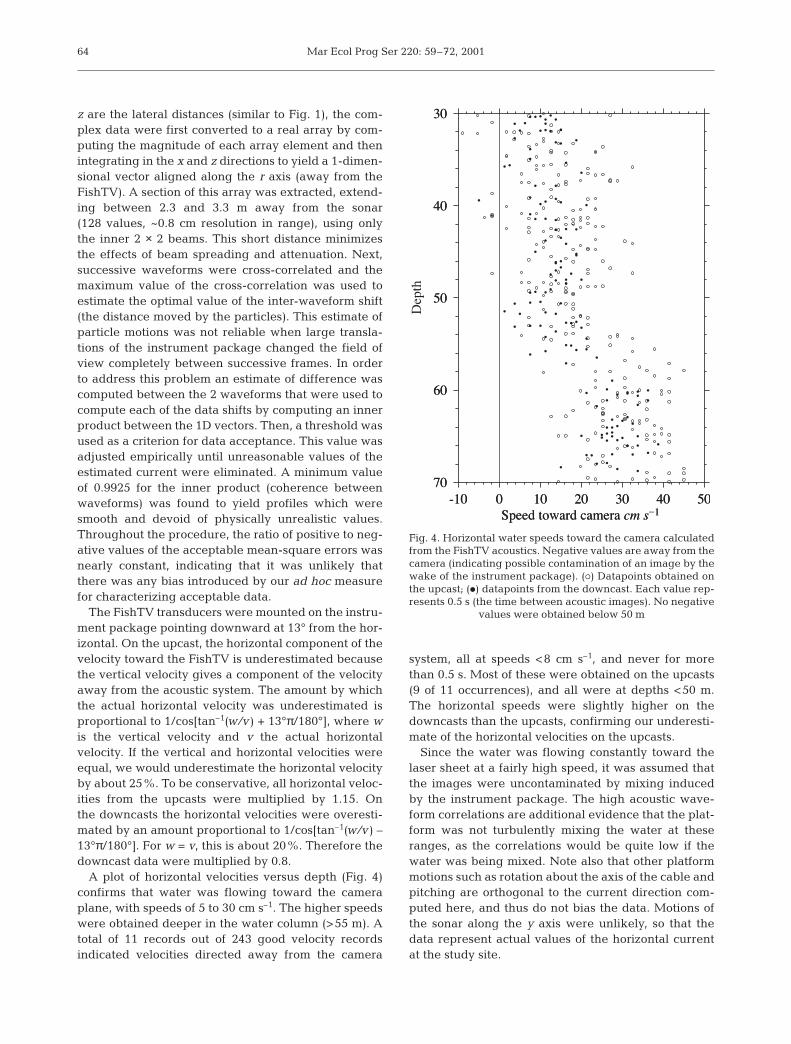
A plot of horizontal velocities versus depth (Fig. 4)confirms that water was flowing toward the cameraplane, with speeds of 5 to 30 cm s–1. The higher speedswere obtained deeper in the water column (>55 m). Atotal of 11 records out of 243 good velocity recordsindicated velocities directed away from the camera

system, all at speeds <8 cm s–1, and never for morethan 0.5 s. Most of these were obtained on the upcasts(9 of 11 occurrences), and all were at depths <50 m.The horizontal speeds were slightly higher on thedowncasts than the upcasts, confirming our underesti-mate of the horizontal velocities on the upcasts.

Since the water was flowing constantly toward thelaser sheet at a fairly high speed, it was assumed thatthe images were uncontaminated by mixing inducedby the instrument package. The high acoustic wave-form correlations are additional evidence that the plat-form was not turbulently mixing the water at theseranges, as the correlations would be quite low if thewater was being mixed. Note also that other platformmotions such as rotation about the axis of the cable andpitching are orthogonal to the current direction com-puted here, and thus do not bias the data. Motions ofthe sonar along the y axis were unlikely, so that thedata represent actual values of the horizontal currentat the study site.

64

Fig. 4. Horizontal water speeds toward the camera calculatedfrom the FishTV acoustics. Negative values are away from thecamera (indicating possible contamination of an image by thewake of the instrument package). (s) Datapoints obtained onthe upcast; (d) datapoints from the downcast. Each value rep-resents 0.5 s (the time between acoustic images). No negative

values were obtained below 50 m

Franks & Jaffe: Microscale distributions of phytoplankton

OSST impulse and frequency response. To inter-pret the spatial variability of fluorescence in theimages, it is necessary to calculate the system’simpulse response and frequency response—the filtercharacteristics of the instrument. If the instrumentwere working perfectly, each pixel would be com-pletely independent of its neighbors. However, thesystem is never perfect, and the information at onepixel is weighted with information from adjacent pix-els. The degree of weighting is known as the impulseresponse, while the Fourier transform of the impulseresponse is the frequency response. The frequencyresponse gives the relative attenuation of variance ateach wavenumber, i.e., the filter characteristics of thesystem (e.g., high-pass, low-pass, etc.). To calculatethe impulse response, we searched through the goodimages for isolated bright pixels, assuming that thesewere fluorescent particles smaller than the resolutionof the camera (delta functions in terms of the camera);25 such pixels were found. Their peaks were aligned,and an average radial fluorescence profile was calcu-lated along the 2 adjacent horizontal and vertical pix-els (Fig. 5a). This 1-dimensional average peak wasused as a convolution kernel to determine the sys-tem’s frequency response. Note that the frequencyresponse is reasonably sensitive to the exact choice ofkernel—slight changes in the values could lead torelatively large changes in the frequency response. AMontecarlo simulation was performed, convolving theimpulse response with random time series, and calcu-lating their spectra (Fig. 5b). The frequency responseshowed the system to behave as a weak low-pass fil-ter: variance decreased at high wavenumbers (smallspatial scales). The roll-off began at 5 to 10 cm scales,with ~60% reduction in variance at 1 cm scales. Withthis frequency response, an underlying white spec-trum would be distorted by our camera system toresemble the spectrum of Fig. 5b—decreasing vari-ance with increasing wavenumber. The standard de-viations shown in Fig. 5b are conservative, given thatthe variance in the impulse response kernel was notincluded in these estimates.

RESULTS AND DISCUSSION

The CTD/fluorometer profiles taken ~1 h prior to and~1 h after the OSST profiles showed a relatively linearincrease of density with depth (Fig. 6). The steppystructure was driven by temperature; within the reso-lution of our CTD, no evidence was found for extensiveoverturns or mixing. The facts that the density profileis quite linear, and the images were acquired wellbelow the seasonal pycnocline at 15 m, suggest thatthe water column was not particularly turbulent.

The fluorescence showed 2 peaks: a broad primarymaximum between 45 and 60 m, and a thinner, intensesecondary maximum between 60 and 68 m. This sec-ondary maximum appeared and disappeared from ourstudy site over about 10 h. Analyses of rates of increaseof chlorophyll suggest that this feature was probably apatch that advected past our anchor station. The plotsof fluorescence versus σT (Fig. 6) show that the fluores-cence peaks remained on their isopycnals (to withinthe resolution of our CTD) throughout the deployment,even though they moved up and down in space. The 4vertical profiles with the OSST were taken over about1 h, and varied little except for offsets due to internalwaves.

A total of 240 images passed the selection criteria,and will be referred to as ‘good’ images. A histogram ofthe frequency of occurrence of good images versusdepth (Fig. 7) shows the images to be relatively evenlyspread between 30 and 68 m depth. Between 5 and 20

65

1

Fig. 5. System (a) impulse and (b) frequency response. If thesystem were perfect, there would be no fluorescence (Fl; arbi-tratry units) at Pixels 1, 2, 4 and 5, only a spike at Pixel 3. Thefrequency response shows the system acts as a weak low-passfilter, reducing the high-wavenumber (short wavelength)variance by as much as 40%. The standard deviations plottedin (b, thin lines) are asymmetric about the mean, although

they may appear otherwise (see also Fig. 11)

Mar Ecol Prog Ser 220: 59–72, 2001

good images were found in each 2 m bin. The low-variance criterion rejected most of the images <30 and>68 m where the fluorescence was low.

To calculate an approximate calibration curve for theOSST, fluorescence values from the WetStar fluoro-meter were compared to the OSST values (Fig. 8). TwoWetStar profiles were used, the first obtained about 1 hprior to the OSST profiles, the second about 1 h after.Fluorescence values were averaged into 2 m bins. The

average fluorescence value for an OSST image wasused in the comparison. As noted in ‘Methods’, thisaverage covers approximately 4.9 l of water. Both CTDcasts give statistically identical calibration curves, al-though more variance is explained by the first cast (r2 =0.56 for the combined casts). Sharp gradients in prop-erties, combined with smearing in the tubing leadingto the WetStar and depth offsets due to internal waves,lead to imperfect alignment of the various profiles and

66

Fig. 6. CTD/fluorometer profiles ob-tained ~1 h prior to (top left graph)and ~1 h after (top right graph) theOSST profiles. Bottom graph: fluo-rescence (µg chl l–1) plotted againstσT for the 2 CTD casts, showing thatthe chlorophyll maxima were con-

fined to iso-pycnal surfaces

Franks & Jaffe: Microscale distributions of phytoplankton

contributes to variability in the calibration curve. Thecalibration fits of Fig. 8 suggest that the OSST wasimaging average chlorophyll concentrations down to0.3 mg m–3, and up to 5 mg m–3.

We are reasonably certain that the fields imaged bythe OSST were uncontaminated by the instrumentitself. This assertion is based on several lines of evi-dence: (1) The imaging plane (laser sheet) was 1 mupstream of the camera package and frame. (2) TheFishTV showed the horizontal velocities to be directedtoward the camera package. The horizontal velocitieswere typically >10 cm s–1 toward the package. Thusmixing of water in the imaging plane would have tohave occurred >1 m away from the package. The highwaveform correlations of the FishTV data show thatthe water was not mixing upstream of the package.(3) Only a wave could propagate against the current tomix water at the imaging plane. The instrument pack-age oscillated with a frequency >>N, the buoyancy fre-

quency. The package would thus generate tur-bulence, not internal waves. The mixed waterwould advect away from the imaging plane inthe direction of the ambient flow. (4) Flow-tanktests with a scale model showed that the packagedid not disturb the flow except within millimetersof the frame, even when the frame was oscil-lating. We are thus confident that the imagespassing the selection criteria show the spatialpatterns of fluorescence as they existed in situ.

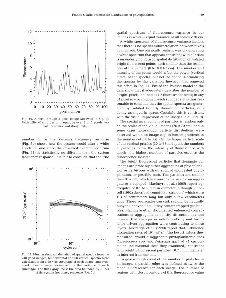
One of our main motivations in designingOSST was the study of the microscale spatialvariability of fluorescence. Fig. 9 shows 4 goodimages, representative of 4 regions of the watercolumn: above the chlorophyll maxima (31.86 m),in the shallow chlorophyll maximum (53.13 m), inthe deeper maximum (64.72 m), and below themaxima (68.43 m). Visual inspection of theseimages reveals a high degree of patchiness offluorescence. A section through the image from64.72 m (Fig. 10) shows changes in fluorescenceof almost an order of magnitude over a few pixelsdistance. These changes are far greater thancould be accounted for by patchiness of materialbetween the imaging plane and the camera (asdiscussed above), and we interpret them to bereal variability in fluorescence. The images pre-sent a ‘starry’ view of fluorescence patchiness—images appear to show many small, isolatedregions of relatively intense fluorescence withlittle structure between these regions. The num-ber and intensity of these regions increases inthe fluorescence maxima. The left-hand edge and

67

Fig. 7. Histogram, top axis: number of good images in each 2 m bin be-tween 31 and 77 m; continuous line, bottom axis: fluorescence (mg chll–1) from a vertical profile of a WetStar fluorometer ~1 h prior to theOSST deployment; (d) average fluorescence (arbitrary units) from all1200 OSST images (note that the average is not affected by smearing),

(s) average fluorescence from 240 good OSST images

Fig. 8. Relationship of OSST fluorescence (arbitrary units) andchlorophyll (mg m–3) estimated from the WetStar fluorometer.Data points are averages of 2 m bins. Two WetStar casts areshown, ~1 h prior to, and ~1 h after the OSST deployment

(see Fig. 6)

Mar Ecol Prog Ser 220: 59–72, 2001

lower-right corner of the images show the edge of thelaser sheet; these regions were not used in any of theanalyses. By rejecting smeared images (criterion givenin ‘Methods’), images with naturally-formed layers inthem might also be rejected. After checking everyrejected image, it was apparent that no obviously lay-ered images were rejected by this criterion, althoughsome images had obvious gradients in the number ofbright pixels from the top to the bottom of the image,particularly images captured at the upper and loweredges of the secondary maximum (e.g., Fig. 9: 68.43 m).

Knowing the system impulse response, it is possibleto interpret spatial spectra calculated from the images.Such spectra should contain important information onthe spatial variability of fluorescence, and potentialclues concerning the dynamics underlying its forma-tion. To address the relationship of fluorescence vari-ability with spatial scale, 64 vertical and 64 horizontal

1D spatial spectra were calculated from a 64 × 64 pixelsubimage in the center of each good image. No statis-tical differences were found between the average ver-tical and horizontal spectra (i.e., the variability wasisotropic). The vertical and horizontal spectra weretherefore averaged to obtain a grand average for eachimage. This average 1D spectrum was divided by thetotal variance of the subimage. If the different imageshave the same spatial structures but different fluores-cence intensities, this scaling should allow the spectrato lie on top of each other. This was the case (Fig. 11),as the mean ± standard deviation of the 240 averagespectra form a tight grouping.

The similarity between the averaged spatial spec-trum calculated from the data (Fig. 11) and the systemfrequency response (Fig. 5b) is striking. Statistically,the 2 spectra are basically indistinguishable, with broadoverlap of the standard deviations at each wave-

68

31.86 m 53.13 m

64.72 m 68.43 m

5

4

3

2

1

0

Fig. 9. Four good imagesof laser-induced fluores-cence (arbitrary units) fromrepresentative regions ofthe water column (see Fig. 6for CTD/fluorometer pro-files). Arrow above 64.72 mimage indicates the slice inFig. 10. Color bar in OSST

units (see Fig. 8)

Franks & Jaffe: Microscale distributions of phytoplankton

number. Since the system’s frequency response(Fig. 5b) shows how the system would alter a whitespectrum, and since the observed average spectrum(Fig. 11) is statistically no different than the systemfrequency response, it is fair to conclude that the true

spatial spectrum of fluorescence variance in ourimages is white—equal variance at all scales <70 cm.

A white spectrum of fluorescence variance impliesthat there is no spatial autocorrelation between pixelsin an image. One physically realistic way of generatinga white spectrum that appears consistent with our datais an underlying Poisson spatial distribution of isolatedbright fluorescent points, each smaller than the resolu-tion of the camera (0.67 × 0.67 cm). The number andintensity of the points would affect the power (verticaloffset) of the spectra, but not the shape. Normalizingthe spectra by the variance, however, has removedthis offset in Fig. 11. Fits of the Poisson model to thedata show that it adequately describes the number of‘bright’ pixels (defined as >2 fluorescence units) in any64 pixel row or column of each subimage. It is thus rea-sonable to conclude that the spatial spectra are gener-ated by isolated brightly fluorescing particles, ran-domly arranged in space. Certainly this is consistentwith the visual impression of the images (e.g., Fig. 9).

The spatial arrangement of particles is random onlyon the scales of individual images (70 × 70 cm), and insome cases non-random particle distributions wereobserved within an image (top-to-bottom gradients inthe numbers of particles). On the larger vertical scaleof our vertical profiles (30 to 68 m depth), the numbersof particles follow the intensity of fluorescence withdepth—the highest numbers of particles occur at thefluorescence maxima.

The bright fluorescent particles that dominate ourimages are probably either aggregates of phytoplank-ton, or herbivores with guts full of undigested phyto-plankton, or possibly both. The particles are smallerthan 0.67 cm, which is a reasonable size for an aggre-gate or a copepod. MacIntyre et al. (1995) report ag-gregates of 0.1 to 2 mm in diameter, although Riebe-sell (1992) described comet-like ‘stringers’ which were10s of centimeters long but only a few centimeterswide. These aggregates can sink rapidly, be neutrallybuoyant, or even float if they contain trapped gas bub-bles. MacIntyre et al. documented enhanced concen-trations of aggregates at density discontinuities andinferred that changes in sinking velocity and turbu-lence-driven aggregation were contributing to theselayers. Alldredge et al. (1990) report that turbulencedissipation rates of 10–7 m2 s–3 (the lowest values theymeasured) would disaggregate phytoplanktonic flocs(Chaetoceros spp. and Nitzschia spp.) of ~1 cm dia-meter (the maximal sizes they examined), consistentwith brightly fluorescent particles <0.7 cm in diameteras inferred from our data.

To give a rough count of the number of particles inan image, a particle edge was defined as twice themodal fluorescence for each image. The number ofregions with closed contours of this fluorescence value

69

Fig. 10. A slice through a good image (arrowed in Fig. 9).Variability of an order of magnitude over 1 or 2 pixels was

not uncommon (arbitrary units)

Fig. 11. Mean ± standard deviation of spatial spectra from the240 good images; 68 horizontal and 68 vertical spectra werecalculated from a 68 × 68 subimage of each image, and aver-aged. Spectra were normalized by the variance of eachsubimage. The thick gray line is the area bounded by ±1 SD

of the system frequency response (Fig. 5b)

Mar Ecol Prog Ser 220: 59–72, 2001

was enumerated in an 80 × 80 pixel subimage of thefull image. Given that particles may be too close to-gether to distinguish by this criterion, the particlecount is probably conservative. The numbers of parti-cles closely followed the chlorophyll fluorescence pro-file. Above the primary chlorophyll maximum therewere 0 to 20 particles l–1. In the primary chlorophyllmaximum there were about 15 to 30 l–1, and 30 to 60 l–1

in the secondary maximum. Fluorescent particles wererare below the secondary maximum (<1 l–1), possiblydue to reduced fluorescence per particle rather thanan absence of particles. Between the primary and sec-ondary chlorophyll maxima, the number of particlesfell to <15 l–1 at about 58 m. These numbers are con-sistent with literature values: for aggregates >0.5 mmin diameter concentrations ranged from 10 to 600 l–1

(Gorsky et al. 1992, MacIntyre et al. 1995, Kiørboe etal. 1998), while aggregates >3 mm tend to be morerare: 1 to 10 l–1 (e.g., Alldredge & Silver 1988). On theother hand, these particle concentrations are muchhigher than would be expected for densities of cope-pods, supporting the contention that most of them aremarine snow aggregates.

The 2 to 3 m thickness of the secondary chlorophyllmaximum makes it slightly thicker than the usual defi-nition of a ‘thin layer’ (<1 m thick; Cowles & Donaghay1998). This layer is not a homogeneous sheet, as layerstend to be envisioned (e.g., Franks 1995; ‘Oceanogra-phy’ special issue on thin layers, Vol. 11(1), 1998), buta layer with a great deal of microscale structure formedby individual particles. The layer could have formedthrough local growth of the particles, or accumulationof the particles through sinking and aggregation at anisopycnal (cf. Derenbach et al. 1979, MacIntyre et al.1995). At the resolution of our data, the layer does notseem to be inclined across isopycnals, and its thin ver-tical extent is probably not due to vertical shearingof an initially thicker layer (cf. mechanism of Franks1995). One scenario consistent with the data is thataggregates formed in and above the primary chloro-phyll maximum (30 to 55 m), and then sank and accu-mulated at the secondary maximum (cf. MacIntyre etal. 1995). The relative absence of fluorescent particlesbelow 68 m could be due to a reduction in the numberof particles, or a marked reduction in fluorescence ofthe particles forming the aggregates. This sinking sce-nario may also explain the lack of acoustic targets atthe depth of the highest chlorophyll fluorescence (Jaffeet al. 1998): the aggregates forming the secondarymaximum may be relatively unpalatable to the herbi-vores. Unfortunately, it is not possible to test this (orother) hypotheses with the data at hand.

The patchiness of fluorescence may also representpatchiness of physiological state of the phytoplankton,rather than variance of biomass on those scales. Given

the many factors that control fluorescence yield inphytoplankton, it is entirely possible that the variabil-ity we have measured represents the scales of phyto-plankton physiological or photosynthetic variability.An instrument such as the fast repetition-rate fluoro-meter (FRRF: Kolber et al. 1998) that could resolvethese spatial scales could help to test such a hy-pothesis.

It is likely that some of the strongly fluorescing parti-cles were crustacean herbivores, and it is possible thatan unexpected benefit of the OSST system will be anability to quantify herbivore gut fluorescence. To dis-tinguish free phytoplankton fluorescence from cope-pod gut fluorescence will require modifications to theOSST system, including higher magnification or thesensing of additional wavelengths (for example back-scattered light).

The lack of a spectral slope in our average spatialspectrum was somewhat surprising to us, given theliterature suggesting that a –5/3 slope would be alikely observation (e.g., Batchelor 1959, Denman &Platt 1976, Denman et al. 1977, Gargett 1985). Thesemodels explore continuous tracers with and withoutgrowth in a 3-dimensional turbulent field. Variance iscreated at large scales and dissipated at small scalesaround the inertial subrange of turbulent mixing.Based on physical observations, we feel that we haveresolved the scales over which we would expect to seean inertial subrange, but we see no evidence of a –5/3slope (or any slope) to the average fluorescence spec-trum. Rather, the spectra are dominated by the contri-bution of relatively rare, isolated, randomly distributedparticles—a quantum phenomenon rather than a con-tinuum phenomenon (see also Siegel 1998). In retro-spect, this should not be so surprising, as a flat spec-trum would be predicted in a region dominated byaggregates. The question remains, then, whether a–5/3 slope would be found in a region without thelarger particulate fluorescence, or with a higher num-ber of particles, and what sort of sampling and statis-tics would be required to resolve the spectrum in aregion of weak, intermittent turbulence.

Potential applications of OSST

Images of the type described here will considerablyexpand the field of study of microscale patchiness ofplankton. Combined with appropriate physical mea-surements (vertical profiles of dissipation of turbulentkinetic energy and dissipation of temperature variance),the spatial information contained in these images willallow testing of hypotheses of physical and biologicalcontrol of microscale structures of the phytoplankton.Theoretical microscale spatial spectra of phytoplank-

70

Franks & Jaffe: Microscale distributions of phytoplankton

ton have included the dynamics of a passive tracer in aturbulent field (e.g., Hinze 1959), simple growth andmixing (Denman & Platt 1976, Denman et al. 1977) andgrowth with mixing and species interactions (grazingand density dependence) (Powell & Okubo 1994). Thesehypothetical spectra have remained largely untestedon the appropriate scales of isotropic turbulence (<1 m,e.g., Gargett 1985) mainly due to technological limita-tions. The deployment of the OSST in a variety of tur-bulence regimes (wind-driven, tidally driven, internal-wave driven, etc.) will allow strong testing of thesemodels, and development of new models should exist-ing ones be rejected.

Testing of such models will require accurate data onthe microscale physical structures and dynamics of theenvironment. Enhancing the OSST with microstruc-ture sensors would enable coincident measurement ofessential physical and biological variables at similarspatial scales. Such physical measurements will sig-nificantly enhance our ability to quantify the temporaland spatial patchiness of the microscale environmentthat the plankton inhabit, and how variability at thesescales influences growth and trophic transfers in theplankton.

The observations of phytoplankton patchiness byOSST can also be used to explore questions of biologi-cal aggregation. This issue has received considerableattention recently (e.g., papers in ‘Deep-Sea Res’ II42(1)1995), and a great deal of effort has been spenttrying to understand the dynamics of aggregation, floc-culation and particle stickiness in relation to phyto-plankton species and densities. Sequences of OSSTimages taken on successive profiles through the devel-opment and decay of a bloom could help to answerquestions concerning the dynamics of aggregate for-mation and the fate of primary production in theoceans.

While numerous laboratory experiments have beenperformed examining the behavioral response of her-bivores to patchiness of phytoplankton (e.g., Tiselius1992, Saiz et al. 1993), little in situ work has been done.Little is known about the microscale structure of thephytoplankton (and by inference the food environmentof the herbivores), and our knowledge of how herbi-vores navigate within this environment is poor. TheOSST will allow investigations of phytoplankton-herbivore interactions on the foraging scales of theorganisms, giving a novel and important new view oftrophic interactions in the sea.

Acknowledgements. This project would not have been suc-cessful without the help of many dedicated people. Particularthanks are due to Greg Adelman and Ed Reuss who did thebulk of the engineering on the OSST and FishTV systems.Mary Sisti cheerfully organized much of the cruise. Cap-

tain Louis Zimm artfully piloted the RV ‘Sproul’, and TammiKoonce, Bob Wilson and Fred Uhlmann were indispensablehelp in deploying the system. Andrew Leising, Alex De-Robertis and Adrienne Huston were a great help in sampling,and Dave Zawada processed many of the raw images. Veryuseful comments on the manuscript were made by JamesPringle and Thomas Kiørboe. Thanks particularly to EricShulenberger, Ron Tipper, Steve Ackleson and Larry Clarkfor encouraging this enterprise.

LITERATURE CITED

Alldredge AL, Silver MW (1988) Characteristics, dynamicsand significance of marine snow. Prog Oceanogr 20:41–82

Alldredge AL, Granata TC, Gotschalk CC, Dickey TD (1990)The physical strength of marine snow and its implicationsfor particle disaggregation in the ocean. Limnol Oceanogr35:1415–1428

Batchelor GK (1959) Small-scale variation of convected quan-tities like temperature in turbulent fluid. J Fluid Mech 5:113–133

Bird JL, Kitting CL (1982) Laboratory studies of a marinecopepod (Temora turbinata Dana) tracking dinoflagellatemigrations in a miniature water column. Contrib Mar Sci25:27–44

Bjornsen PK, Nielsen TG (1991) Decimeter scale heterogene-ity in the plankton during a pycnocline bloom of Gyro-dinium aureolum. Mar Ecol Prog Ser 73:263–267

Bohrer RN (1980) Experimental studies on diel vertical migra-tion. In: Kerfoot W (ed) Evolution and ecology of zoo-plankton communities. University Press of England, Lon-don, p 111–121

Cowles TJ, Donaghay P (1998) Thin layers: observations ofsmall-scale patterns and processes in the upper oceanOceanography 11:2

Cowles TJ, Fessenden LM (1995) Copepod grazing and fine-scale distribution patterns during the marine light-mixedLayers experiment. J Geophys Res 100:6677–6686

Cowles TJ, Desiderio RA, Neuer S (1993) In situ characteriza-tion of phytoplankton from vertical profiles of fluores-cence emission spectra. Mar Biol 115:217–222

Derenbach JB, Astheimer H, Hansen HP, Leach H (1979) Ver-tical microscale distribution of phytoplankton in relation tothe thermocline. Mar Ecol Prog Ser 1:187–193

Denman KL, Platt T (1976) The variance spectrum of phyto-plankton in a turbulent ocean. J Mar Res 34:593–601

Denman KL, Okubo A, Platt T (1977) The chlorophyll fluctua-tion spectrum in the sea. Limnol Oceanogr 22:1033–1038

Desiderio RA, Cowles TJ, Moum JN, Myrick M (1993) Micro-structure profiles of laser-induced chlorophyll fluorescencespectra: evaluation of backscatter and forward-scatterfiber-optic sensors. J Atmos Oceanic Technol 10:209–224

Franks PJS (1995) Thin layers of phytoplankton: a model offormation by near-inertial wave shear. Deep-Sea Res I42:75–91

Gargett AE (1985) Evolution of scalar spectra with the decayof turbulence in a stratified fluid. J Fluid Mech 159:379–407

Gorsky G, Aldorf C, Kage M, Picheral M, Garcia Y, Favole J(1992) Vertical-distribution of suspended aggregatesdetermined by a new underwater video profiler. Ann InstOcéanogr 68:275–280

Hinze JO (1959) Turbulence. McGraw Hill, New YorkJaffe JS (1999) Target localization for a three-dimensional

multibeam sonar imaging system. J Acoust Soc Am 105:3168–3175

71

Mar Ecol Prog Ser 220: 59–72, 2001

Jaffe JS, Ruess E, McGeehee D, Chandran G (1995) FTV— asonar for tracking macrozooplankton in 3 dimensions.Deep-Sea Res I 42:1495–1512

Jaffe JS, Franks PJS, Leising AW (1998) Simultaneous imag-ing of phytoplankton and zooplankton distributions. Oce-anography 11:24–29

Kiørboe T, Tiselius P, Mitchell-Innes B, Hansen JLS, VisserAW, Mari X (1998) Intensive aggregate formation with lowvertical flux during an upwelling-induced diatom bloom.Limnol Oceanogr 43:104–116

Kolber ZS, Prasil O, Falkowski PG (1998) Measurements ofvariable chlorophyll fluorescence using fast repetition ratetechniques: defining methodology and experimental pro-tocols. Biochim Biophys Acta-Bioenergetics 1367:88–106

MacIntyre S, Alldredge AL, Gotschalk CC (1995) Accumula-tion of marine snow at density discontinuities in the watercolumn. Limnol Oceanogr 40:449–468

McGeehee D, Jaffe JS (1996) Three-dimensional swimmingbehavior of individual zooplankters: observations usingthe acoustical imaging system FishTV. ICES J Mar Sci 53:363–369

Morel A (1988) Optical modeling of the upper ocean in rela-tion to its biogenous matter content (Case I waters). J Geo-phys Res 93:10749–10768

Owen RW (1989) Microscale and finescale variations of smallplankton in coastal and pelagic environments J Mar Res47:197–240

Palowitch AW, Jaffe JS (1994) Three-dimensional ocean chlo-rophyll distributions from underwater serial-sectionedfluorescence images. Appl Optics 33:3023–3033

Palowitch AW, Jaffe JS (1995) Optical serial sectioned chloro-phyll-a microstructure. J Geophys Res 100:13267–13278

Powell TM, Okubo A (1994) Turbulence, diffusion and patchi-ness in the sea. Philos Trans R Soc Lond B Biol Sci 343:11–18

Price H (1989) Swimming behavior of krill in response toalgal patches: a mesocosm study. Limnol Oceanogr 34:649–659

Riebesell U (1992) The formation of large marine snow and itssustained residence in surface waters Limnol Oceanogr37:63–76

Saiz E, Tiselius P, Jonsson PR, Verity P, Paffenhöfer GA (1993)Experimental records of the effects of food patchinessand predation on egg production of Acartia tonsa. LimnolOceanogr 38:280–289

Siegel DA (1998) Resource competition in a discrete environ-ment: why are plankton distributions paradoxical? LimnolOceanogr 43:1133–1146

Sutton DW, Jaffe JS (1992) Acoustic bedload velocity esti-mates using a broadband pulse-pulse time correlationtechnique. J Acoust Soc Am 92:1692–1698

Tiselius P (1992) Behavior of Acartia tonsa in patchy foodenvironments Limnol Oceanogr 37:1640–1651

Tiselius P, Nielsen G, Nielsen TG (1994) Microscale patchi-ness of plankton within a sharp pycnocline. J Plankton Res16:543–554

Welch PD (1967) The use of fast Fourier transform for the esti-mation of power spectra: a method based on time averag-ing over short modified periodograms. IEEE (Inst ElectElectron Eng) Trans Audio Electroacoust 15:70–73

72

Editorial responsibility: Otto Kinne (Editor), Oldendorf/Luhe, Germany

Submitted: July 13, 2000; Accepted: December 12, 2000Proofs received from author(s): August 29, 2001