1

A Modelling Assessment of Contaminant Distributions

in the Severn Estuary

Murdoch1,*, N. , Jonas1, P.J.C., Falconer2, R. A., Lin2, B.

1Environment Agency, Manley House, Kestrel Way, Exeter, EX2 7LQ Devon, UK

2School of Engineering, Cardiff University, The Parade, CARDIFF CF24, 3AA, UK

Abstract

The regulatory requirements imposed by the Habitats Directive (EU

93/43/EEC) require the Environment Agency for England and Wales (EA) to

review consented discharges and determine whether they are compliant with

Environmental Quality Standards (EQS). Since the EQS are annual averages,

model predictions, and sample comparisons, should be made on an annual

average basis. Advection and dispersion of metal contaminants in the Severn

Estuary were computed using a coupled 1-D and 2-D hydrodynamic-water

quality model. The external inputs of dissolved copper, arsenic, mercury and

chromium to the model were from 66 industrial discharges and sewage

treatment works and 30 rivers. The annual average predicted concentrations

were compared with the annual average dissolved metal concentrations from

the 2004 and 2005 monitoring programme, and any discrepancy used to

identify the role of additional processes, mainly involving the sediments. This

ability to separate anthropogenic inputs from internal estuarine processes

contributes to a better understanding of the functioning of the estuary and

hence an improved management capability. The paper discusses the

approach in designing scenarios and characterising uncertainty, when

decision-making in the regulatory context.

Keywords Severn, water quality, metals, numerical modelling, regulation

* Address for correspondence: e-mail Neil.Murdoch@Environment-Agency.Gov.UK

2

1. Introduction

Water quality in the Severn Estuary is subject to influences from many

sources. The major rivers, including the Severn, Wye, Bristol Avon, Usk, Taff

and Parret with a combined annual mean flow of 275 m3 s-1 deliver metal

contaminants from their catchments into the estuary (Fig. 1). An additional 24

smaller rivers with a combined annual mean flow of 155 m3 s-1 add to the

contaminant load. Direct discharges, with a combined annual mean flow of 16

m3 s-1 from industry and sewage treatment works, complete the inventory of

external loadings to the estuary. Generally, rivers supply a greater proportion

of the nutrient load, whilst dissolved metals appear to be dominated by the

direct discharges (Jonas and Millward, this volume). Metals exist either bound

to suspended particulate material (SPM) or as dissolved species, with their

relative proportions being characterised by a partition coefficient, which

depends to a large extent on estuarine chemistry (Turner and Millward, 2002).

Dissolved and particulate concentrations of metals are also influenced by

hydrodynamic processes of dilution, advection and dispersion. Although

recent research suggests that metal concentrations in sediments from the

estuary are declining (Duquesne et al., 2006; Langston et al., 2007; this

volume), in some cases they may be acting as an additional internal source of

or sink for metals (Jonas and Millward, this volume).

The hydrodynamics and water circulation of the Severn Estuary and

Bristol Channel are the main agents for the dispersion and dilution of

contaminants. Previous modelling studies of contaminants in the Severn have

examined the distributions of cadmium (Radford et al., 1981) and caesium-

137 (Uncles, 1979; Rattray and Uncles, 1983). In a study aimed at predicting

the distributions of caesium-137, Rattray and Uncles (1983) developed a 1-

dimensional (D) model that showed that the dispersion characteristics for

salinity and a non-conservative tracer were similar and this could be used to

predict estuarine concentrations from defined sources. Radford et al (1981)

developed a 1-D tidally averaged model which was used to estimate the

advective and dispersive properties of the estuary. Estimates of the known

cadmium loads to the estuary, at the time, were then used to predict estuarine

concentrations of dissolved cadmium. Comparison of the computer

simulations with concentrations of dissolved cadmium in the estuary (i.e. 30

3

axial transects) showed the crucial importance of establishing accurate and

precise values for the magnitudes of the input loads and hence the need for

consistently monitored sources was emphasised.

There has been significant development of various numerical models

(Uncles, this volume) for the system, for example a 3-D model, used to predict

tidal and residual currents in the Severn Estuary, was developed by Wolf

(1987). Recently Yang et al. (2008) applied a 2-D model to the prediction of

enteric bacteria distributions in the Severn Estuary. A conceptual model

representing the transport of bacteria due to sediment movement was

developed, including deposition and suspension and the effect of sediment on

the transport and decay of enteric bacteria. The basis of the code developed

by Yang et al. (2008) was the DIVAST model (Lin and Falconer, 1997; 2001)

which is a coupled hydrodynamic-water quality model that has been widely

applied in the UK and overseas. For example, a 2-D version has been used to

model trace metal concentrations in the Mersey estuary (Wu et al., 2005).

Also, Delaney et al. (2007) have incorporated DIVAST into a GIS expert

system for habitat management in estuarine systems. A 3-D version of the

model has previously been applied to the Severn Estuary (Lin and Falconer,

2001). Numerical modelling is becoming more important in the decision-

making process, although Jones et al. (2002) provided a critical review of the

role of models in estuarine management.

Here we used the established DIVAST model with a view to examining

the fate of discharge and river loadings mainly with respect to advection and

dispersion processes, in a similar way to Radford et al. (1981). This is a

cautious approach in that sediment resuspension processes, including

sediment-water interactions, are not included in the model. However, this is

not to say that they are not relevant or that the model is incapable of

representing them, rather it is considered essential, from an estuary

management perspective, to separate out the contributions to dissolved

concentrations from the discharges directly from any estuarine geochemical

processes. This separation is achieved by comparing the model predictions

with measurements of the dissolved concentrations of metals in the estuary.

This approach allows identification of potential geochemical processes that

require further investigation.

4

The aim of the present study is to evaluate the impact on the estuarine

concentrations of the dissolved metal releases from the currently monitored

rivers and discharges. The unique contribution of this work is that for the first

time the combined effect of a large number of discharges and rivers impacting

on the Severn are examined, which would be very difficult, if not impossible,

without the aid of a numerical model. The results of this study could then be

used to assess whether the estuarine concentrations resulting from the

discharges are compliant with the Environmental Quality Standards (EQS) as

required by the Habitats Directive.

5

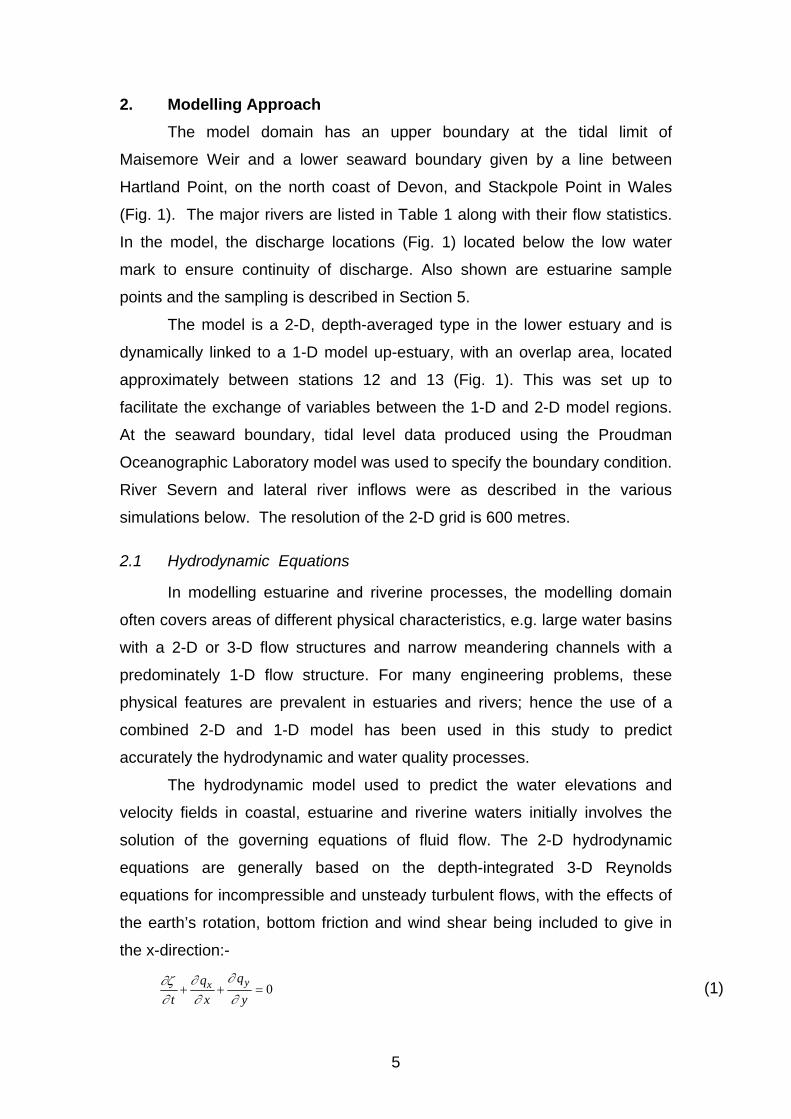
2. Modelling Approach

The model domain has an upper boundary at the tidal limit of

Maisemore Weir and a lower seaward boundary given by a line between

Hartland Point, on the north coast of Devon, and Stackpole Point in Wales

(Fig. 1). The major rivers are listed in Table 1 along with their flow statistics.

In the model, the discharge locations (Fig. 1) located below the low water

mark to ensure continuity of discharge. Also shown are estuarine sample

points and the sampling is described in Section 5.

The model is a 2-D, depth-averaged type in the lower estuary and is

dynamically linked to a 1-D model up-estuary, with an overlap area, located

approximately between stations 12 and 13 (Fig. 1). This was set up to

facilitate the exchange of variables between the 1-D and 2-D model regions.

At the seaward boundary, tidal level data produced using the Proudman

Oceanographic Laboratory model was used to specify the boundary condition.

River Severn and lateral river inflows were as described in the various

simulations below. The resolution of the 2-D grid is 600 metres.

2.1 Hydrodynamic Equations

In modelling estuarine and riverine processes, the modelling domain

often covers areas of different physical characteristics, e.g. large water basins

with a 2-D or 3-D flow structures and narrow meandering channels with a

predominately 1-D flow structure. For many engineering problems, these

physical features are prevalent in estuaries and rivers; hence the use of a

combined 2-D and 1-D model has been used in this study to predict

accurately the hydrodynamic and water quality processes.

The hydrodynamic model used to predict the water elevations and

velocity fields in coastal, estuarine and riverine waters initially involves the

solution of the governing equations of fluid flow. The 2-D hydrodynamic

equations are generally based on the depth-integrated 3-D Reynolds

equations for incompressible and unsteady turbulent flows, with the effects of

the earth’s rotation, bottom friction and wind shear being included to give in

the x-direction:-

0yx qq

t x y

(1)

6

2 2

2 2x x x xw xb

yq Uq Vq U U

fq gH Ht x y x x y

(2)

where hH = total water column depth; = water elevation above (or

below) datum; h = water depth below datum; VU , = depth-averaged velocity

components in yx, directions; VHqUHq yx , = unit width discharge

components (or depth integrated velocities) in yx, directions; = momentum

correction factor; f = Coriolis parameter; g = gravitational acceleration; xw =

surface wind shear stress components in x direction; xb = bed shear stress

components in x directions; and = depth average eddy viscosity.

A similar equation can be developed for the y-direction as to that given

for the x direction (i.e. Equation 2). Likewise for the 1-D river flow equation

assumed that the St Venant hypotheses were valid and the corresponding

conservation of mass and momentum equations for the 1-D flows were

represented as:

0

x

Q

tT RR (3)

2

20R RR R R

z

Q QQ QgA g

t x A x C AR

(4)

where T = top width of the channel; R = water elevation above (or below)

datum; RQ = discharge; = momentum correction factor due to the non-

uniform velocity over the cross section; A = wetted cross-sectional area;

PAR / = hydraulic radius and P = wetted perimeter of the cross-section.

2.2 Contaminant Transport

Contaminant transport may be described by the following two

dimensional advection dispersion equation:-

sourceskCy

CHDy

yx

CHD

xCq

yCq

xHC

t xyx

(5)

< ----advection-------------- > < ------dispersion----------- > <-loss->

7

where C is the contaminant concentration, Dx and Dy are the respective x and

y dispersion coefficients, k is a loss term. The sources term in Equation 5

represents the external sources arising from the rivers and discharges but

does not indicate suspended sediment sources (or sinks). For metals, a more

sophisticated treatment based on phase partitioning may be developed (Wu et

al., 2005), although in the present study this was not included, as mentioned

above. The loss term is generic and is not intended to indicate a specific loss

mechanism and is discussed further in Section 3.

2.3 Model Spin-up

Model spin-up is the time taken for modelled estuarine concentrations

to reach equilibrium and is related to the estuarine water retention time. For

the Severn Estuary this has been estimated to be between 90 and 200 days.

Figure 2 shows the time series of model concentrations (for a conservative

determinant, with constant fluvial inputs) in the upper estuary. The spring–

neap cycles are clearly evident and the model begins to, but does not

completely, equilibrate after 7 spring-neap cycles. Thus, a spin-up period of

90 days was used and only dissolved metal concentrations after this were

taken as representative. This period is similar to the estimated flushing time

for the estuary derived by Uncles (1984; this volume).

8

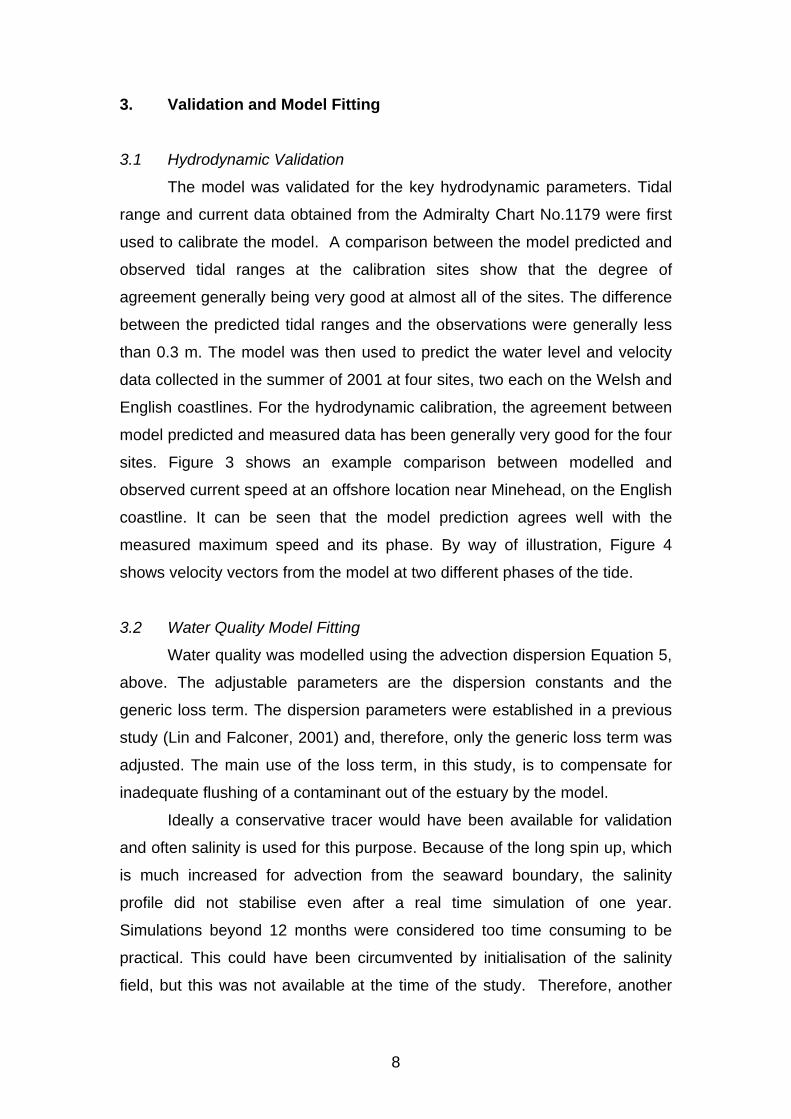
3. Validation and Model Fitting

3.1 Hydrodynamic Validation

The model was validated for the key hydrodynamic parameters. Tidal

range and current data obtained from the Admiralty Chart No.1179 were first

used to calibrate the model. A comparison between the model predicted and

observed tidal ranges at the calibration sites show that the degree of

agreement generally being very good at almost all of the sites. The difference

between the predicted tidal ranges and the observations were generally less

than 0.3 m. The model was then used to predict the water level and velocity

data collected in the summer of 2001 at four sites, two each on the Welsh and

English coastlines. For the hydrodynamic calibration, the agreement between

model predicted and measured data has been generally very good for the four

sites. Figure 3 shows an example comparison between modelled and

observed current speed at an offshore location near Minehead, on the English

coastline. It can be seen that the model prediction agrees well with the

measured maximum speed and its phase. By way of illustration, Figure 4

shows velocity vectors from the model at two different phases of the tide.

3.2 Water Quality Model Fitting

Water quality was modelled using the advection dispersion Equation 5,

above. The adjustable parameters are the dispersion constants and the

generic loss term. The dispersion parameters were established in a previous

study (Lin and Falconer, 2001) and, therefore, only the generic loss term was

adjusted. The main use of the loss term, in this study, is to compensate for

inadequate flushing of a contaminant out of the estuary by the model.

Ideally a conservative tracer would have been available for validation

and often salinity is used for this purpose. Because of the long spin up, which

is much increased for advection from the seaward boundary, the salinity

profile did not stabilise even after a real time simulation of one year.

Simulations beyond 12 months were considered too time consuming to be

practical. This could have been circumvented by initialisation of the salinity

field, but this was not available at the time of the study. Therefore, another

9

determinant, oxidised nitrogen, was used as data were available for all the

inputs, i.e. discharges and rivers, and the estuarine sample points.

The suitability of oxidised nitrogen for model calibration depends on to

what extent it is acting conservatively. Conservative behaviour implies that the

de-nitrification rate is zero and it will not contribute to the loss term (Equation

5) which may then be unambiguously interpreted as compensating for

inadequate flushing. De-nitrification losses have been much discussed in the

literature. From an assessment of a number of estuaries Nixon et al. (1996)

suggested that net nitrification losses were proportional to the logarithm of the

residence time, with losses less than 20% for retention times of 1 month or

less, rising to 40% for 10 month (300 days) retention times. There was

variability in the data and losses as low as 10% were indicated for 10 month

residence time. In a study of the Humber estuary, Barnes et al. (1999)

reported 25% nitrogen loss for a 6 week residence time. In a more recent

study on the Humber (Tappin et al., 2003) found that denitrification was small

and all consequently all nitrate added to the estuary was lost to the sea.

Neilsen et al. (1995) reported loses as low as 3% for a short residence time

estuary in Denmark and they also suggested that net losses of >40% may be

over estimated.

Examination of the variation of the observed estuarine concentrations

of oxidised nitrogen estuarine with salinity should reveal the presence of

source and loss processes. The EA collected water samples for dissolved

metal analysis (and other analytes), at near high water, during axial transects

of the Severn Estuary, involving the same fixed sampling stations, in August,

September and November 2004 and March, June, August and September

2005 (Jonas and Millward, this volume). Figure 5a shows that the annual

average concentrations of oxidised nitrogen, obtained from the axial

transects, vary inversely with salinity. The approximate linear relationship

suggests that losses processes are not playing a significant role and the

nitrogen appears to be behaving approximately conservatively. Considering

the empirical evidence from Figure 5a it seems that the nitrogen losses over

100 day water retention time are low and, consistent with the literature, a

lower end value of less than 15% is estimated.

10

The model predictions for estuarine concentrations of oxidised nitrogen

were compared with the sample data. For the comparison, the model was run

with constant input values for river and discharge flows and concentrations

chosen so as to generate the annual average response within the estuary; the

method for selecting these input values is described in Section 4, below. The

model was run for 90 days spin up and then over a spring-neap cycle with the

prediction data being taking from the spring-neap period The results were

compared with the annual averages of the corresponding sample data and

both are shown in Figure 5b, as a function of distance down-estuary from the

tidal limit. The dashed line is the annual average predicted by the model over

the spring to neap tidal period. The upper envelop indicates the maximum

concentrations during the period, at low water, whilst the lower line shows the

minima at high water. Since the water samples were generally taken as near

high water as practical the appropriate comparator is the lower model line.

This line was fitted by adjusting the loss constant k.

The value of k used in the computations corresponded to an e-folding

time of 50 days, i.e. the loss term in Equation 5 where the concentration is

reduced by 63% in 50 days and 87% in a 100 days. This is far in excess of

the estimated loss by de-nitrification which is 15% over 100 days. Therefore

the loss term is primarily compensating for inadequate model flushing and to a

lesser extent reflecting de-nitrification. In the subsequent simulations for the

dissolved metals below, the same value of k is used. As part of this k is not

attributable to hydrodynamic processes (i.e. to de-nitrification) there is an

uncertainty in the model water quality predictions of about 15% arising from

the advection dispersion representation. In summary the model has been set

up to dilute, advect and disperse contaminant inputs throughout the estuary

with an uncertainty of 15% for annual average predictions.

11

4. Model Scenario Design

The context in which this study originated was regulatory and it is

important to reflect on the significance for modelling. Regulatory organisations

use EQS to control contaminant levels in the environment and hence to

control discharges to the environment. The EQS are expressed in statistical

form as a percentile or annual average; and sometimes as a maximum.

Appropriate percentile standards will control short term impacts whilst annual

averages address the long term problem. From a regulatory perspective

modelling is simply a calculation to determine whether or not there is

compliance with a particular EQS.

This focus on EQS has influenced the approach to modelling. In

freshwater modelling in England and Wales, the regulatory paradigm is

statistical modelling using Monte-Carlo techniques (Crabtree et al., 2006;

Daldorph et al., 2007; Warn, 2003). This allows a direct comparison between

model predictions and the EQS, since they are both expressed in statistical

form. The approach adopted in the marine modelling field has been different,

due in part to the greater complexity implicit in numerical codes (e.g. finite

difference/finite element) where the emphasis has been decidedly

deterministic and process based. Models have been used in the regulatory

context, but more to provide illustrations surrounding specific events than to

couple to the EQS concept. To some extent this has limited the application of

marine models in this area.

Matching marine model output to an EQS is not straightforward and is

often avoided. This is because EQS statistics, whether percentiles or annual

means, (usually) apply over an annual time period. By contrast marine

modelling has to some extent pursued greater sophistication in process

representation which entails longer runs times and so annual runs are often

not undertaken outside of the research environment. The result is a tendency

for episodic event simulation and no link is established between the model

outputs and an EQS.

Because of long run times scenarios are constructed with fixed

freshwater and discharge inputs and run over a spring-neap cycle rather than

a full year. This approach is adopted here. The problem of linking the EQS to

the fixed inputs is addressed using the ‘justified design evaluation method’

12

(Murdoch, 2001). The approach identifies percentiles of the input variables

(flow and concentrations) which drive an annual average response in the

estuary. Here river and discharge flow and concentration data are

represented by lognormal distributions and the identified percentiles are used

to select the fixed input values from these distributions. Table 2 lists the

percentiles so derived and used in this study. There is uncertainty in scenario

definition. This arises from the sampling errors characterising the discharge

and river flow and quality distributions and in identifying the percentiles to fix

the input values. The errors here were estimated at around 20%. Having

calibrated the model, considered the uncertainties and selected the inputs the

model set up process was complete.

13

5. Results and Discussion

Model runs were performed for dissolved copper, arsenic, mercury amd

chromium, with the seaward boundary concentrations set at zero for each

metal. The model was spun up for 90 days and then a spring to neap cycle

run from which the axial concentrations were obtained. All discharge and river

flow concentrations were at fixed values derived as described in Section 4.

The advection-dispersion Equation (5), with the loss term mainly

compensating for inadequate model flushing was employed. Therefore, the

model predictions are primarily the result of (conservative) hydrodynamic

processes with a combined uncertainty of 30% arising from the discussion in

Sections 3 and 4. The model predictions were compared with the annual

average concentrations of the dissolved metals calculated from seven axial

transects, described in Section 3.2.

The results are shown in Figure 6 where the predictions of the annual

average metal concentrations are compared with those observed in the

monitoring programme. The profile of the mean suspended particulate matter

concentrations (SPM) is also shown for interpretative purposes.

Copper: The observed concentrations of dissolved copper are highly variable,

particularly in the upper estuary, and decrease down-estuary. Part of the

variability arises because in August 2005, the dissolved copper

concentrations exceeded the EQS from the freshwater reaches to about 70

down-estuary (Jonas and Millward, this volume). Consequently, the model fits

to the observations vary down-estuary (Fig. 6a), such that up to 20 km down-

estuary the model gives higher values than the observed concentrations. This

is followed by a region between 20 and 60 where there is better agreement

between the predictions and the observations. After about 60 km down-

estuary, the model predictions are higher than the observed concentrations.

The variable agreement between the predictions and observations suggests

other processes, involving metal exchanges between the dissolved and

particulate phases, including net fluxes of dissolved copper from the sediment

porewaters.

14

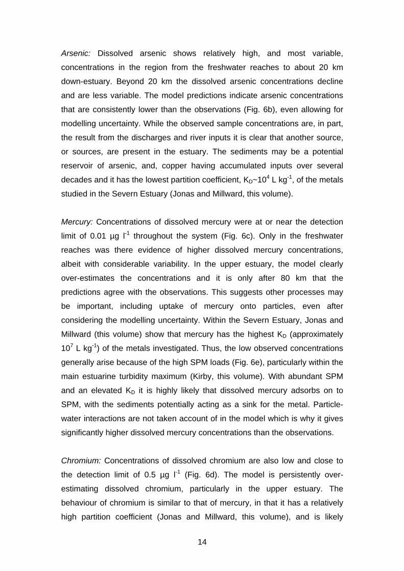
Arsenic: Dissolved arsenic shows relatively high, and most variable,

concentrations in the region from the freshwater reaches to about 20 km

down-estuary. Beyond 20 km the dissolved arsenic concentrations decline

and are less variable. The model predictions indicate arsenic concentrations

that are consistently lower than the observations (Fig. 6b), even allowing for

modelling uncertainty. While the observed sample concentrations are, in part,

the result from the discharges and river inputs it is clear that another source,

or sources, are present in the estuary. The sediments may be a potential

reservoir of arsenic, and, copper having accumulated inputs over several

decades and it has the lowest partition coefficient, KD~104 L kg-1, of the metals

studied in the Severn Estuary (Jonas and Millward, this volume).

Mercury: Concentrations of dissolved mercury were at or near the detection

limit of 0.01 µg l-1 throughout the system (Fig. 6c). Only in the freshwater

reaches was there evidence of higher dissolved mercury concentrations,

albeit with considerable variability. In the upper estuary, the model clearly

over-estimates the concentrations and it is only after 80 km that the

predictions agree with the observations. This suggests other processes may

be important, including uptake of mercury onto particles, even after

considering the modelling uncertainty. Within the Severn Estuary, Jonas and

Millward (this volume) show that mercury has the highest KD (approximately

107 L kg-1) of the metals investigated. Thus, the low observed concentrations

generally arise because of the high SPM loads (Fig. 6e), particularly within the

main estuarine turbidity maximum (Kirby, this volume). With abundant SPM

and an elevated KD it is highly likely that dissolved mercury adsorbs on to

SPM, with the sediments potentially acting as a sink for the metal. Particle-

water interactions are not taken account of in the model which is why it gives

significantly higher dissolved mercury concentrations than the observations.

Chromium: Concentrations of dissolved chromium are also low and close to

the detection limit of 0.5 µg l-1 (Fig. 6d). The model is persistently over-

estimating dissolved chromium, particularly in the upper estuary. The

behaviour of chromium is similar to that of mercury, in that it has a relatively

high partition coefficient (Jonas and Millward, this volume), and is likely

15

adsorbed from solution in the the turbid regions of the estuary (Fig. 6e). As is

the case with mercury, it appears that the sediments are acting as a sink for

chromium.

In summary, comparing the profiles of the concentrations of dissolved

metals with the SPM concentrations, the clearest indication of the influence of

the high SPM load are for mercury and chromium, For both these elements

the main SPM maximum identifies with the largest discrepancy between the

model over-prediction and the observations. This is consistent with the high

partition coefficients for these metals which resulted in lower dissolved

concentrations.

From the regulatory point of view it is reassuring that both the observed

and model predictions are within the values for the individual EQSs (Table 3),

with the exception of copper in August 2005. The sample data were mainly

compliant with the EQS (86% of the total discharge load was in dissolved

phase). The most interesting aspects here are in fact the discrepancies. By

separating out the influences of the discharges the role played by the

sediments begins to emerge. It is not claimed here that a full understanding

has been developed but the model ahs revealed potential sedimentary

influences that need to be clarified by further research. This is relevant to the

long term prognosis with or without a Severn Barrage; that is whether, in the

long-tem, the estuarine sediments will act as a source or sink of dissolved

metals.

16

6. Summary and Conclusion

The fate of external loadings of four dissolved metals from a large number

of discharges and rivers into the Severn Estuary has been investigated. The

combined application of a numerical modelling and sampling provides a

powerful tool to disentangle the role of suspended sediment sources and

sinks from the external loadings. Mercury and chromium appear to be

removed to the particulate phase and, therefore, the sediments act,

potentially, as a sink. Copper and arsenic have relatively low partition

coefficients and appear more geochemically mobile than mercury and

chromium, with proportionally more metal in the dissolved phase. Since

particulate copper and arsenic are labile they are potentially desorbed into

anoxic porewaters and are, therefore, available for remobilisation into the

overlying water column. For copper and arsenic, it appears that the sediments

are acting as a source of dissolved metal.

The focus on annual averages has been driven by regulatory concerns

over EQS. From the regulatory perspective the model and sample results

suggest compliance with the EQS, which are annual averages; this is not to

meant to imply that individual sample concentrations will always be less than

EQS but only that on an annual averaged basis is this the case.

The implications for the modelling community from this study are that

greater attention to simulation outputs being compatible with EQS will help the

regulator. Further clarity on the modelling uncertainty and the long term

contaminant budget ( i.e. input/output loads) are important requirements.

As far as the Severn is concerned further research on seasonal and

annual load budgets and the interplay of external and internal loadings would

help us to better understand the long term evolution of the system. This paper

offers a beginning on this.

Acknowledgements

The Environment Agency (South West) acknowledges MarCon Computations

International for developing the GIS interface under contract. The views

expressed here are not necessarily those of the Environment Agency.

17

References

Barnes, J., Owens, N.J.P., 1999. Denitrification and nitrous oxide concentrations in the Humber Estuary, UK and adjacent coastal zones. Marine Pollution Bulletin 37, 247-260.

Crabtree, B., Seward, A.J., Thompson, L., 2006. A case study of regional catchment water quality modelling to identify pollution control requirements. Water Science and Technology 53, 47-54.

Daldorph, P.W.G., Spraggs, G.E., Lees, M.J., Wheater, H.S., Chapra, S.C., 2007. Integrated lake and catchment phosphorus model -A eutrophication management tool. II: Application to Rutland Water. Water and Environment Journal 15, 182-189.

Delaney, C., Berry, A., Hartnett, M., Simmons, P., 2007. A description of a sophisticated GIS based expert system for use in habitat management in dynamic estuarine environments. Proceedings of the 8th International Symposium on GIS and Computer Mapping for Coastal Zone Management, Vol 2, 413-423.

Duquesne, S., Newton, L.C., Giusti, L., Marriott, S.B., Stark,H.J.,Bird, D.J., 2006. Evidence for declining levels of heavy-metals in the Severn Estuary and Bristol Channel, U.K. and their spatial distribution in sediments. Environmental Pollution 143,187-196.

Falconer, R.A., Lin B., Wu, Y., Harris, E., (2001). DIVAST Reference Manual, Manual, Environmental Water Management Research Centre, Cardiff University.

Jones, P.D., Tyler, A.O., Wither, A.W., 2002. Decision-support Systems: Do they have a future in estuarine management? Estuarine, Coastal and Shelf Science 55,993-1008.

Langston, W.J., Chesman, B.S., Burt, G.R., Campbell, M., Manning A.J., Jonas, P.J.C., 2007. The Severn Estuary: Sediments, Contaminants and Biota. Marine Biological Association of the UK Occasional Publication, No. 19, 176 pp.

Langston, W.J., Millward, G.E., 2008. Review of Contaminant Levels in the Severn Estuary SAC, SPA, Plymouth Marine Science Partnership, July 2008, 95 pp.

Lin, B., R.A. Falconer, 1997. Tidal flow and transport modelling using the ULTIMATE QUICKEST scheme, Journal of Hydraulic Engineering ASCE 123, 303-314.

Lin, B., Falconer, R.A., 2001. Numerical modelling of 3-D tidal currents and water quality indicators in the Bristol Channel. Proceedings of Institution of Civil Engineers, Water and Maritime Engineering 148,155-166.

Murdoch, N., 2001, Justified design evaluation for percentile standards, Environmental Modellling and Software 16, 725-738.

Neilsen, K., Nielsen, L.P., Rasmussen P., 1995. Estuarine nitrogen retention independently estimated by denitrification rate and mass balance methods: a study of Norsminde Fjord, Denmark, Marine Ecology Progress Series 119, 275-283.

Nixon, S.W., Ammerman, J.W., Atkinson, L.P., Berounsky, V.M., Billen, G., Boicourt, W.C., Boynton, W.R., Church, T.M., DiToro, D.M., Elmgren, R., Garber, J.H., Giblin, A.E., Jahnke, R.A., Owens, N.J.P., Pilson, M.E.Q., Seitzinger, S.P., 1996. The fate of nitrogen and phosphorus at the land-sea margin of the North Atlantic Ocean. Biogeochemistry 35, 141-180.

18

Radford, P.J., Uncles, R.J., Morris, A.W., 1981. Simulating the impact of technological change on dissolved cadmium distribution in the Severn estuary, Water Research 15, 1045-1052.

Rattray M., Uncles R.J., 1983. On the predictability of the 137Cs distribution in the Severn Estuary, Estuarine, Coastal and Shelf Science16, 475-487.

Turner, A., Millward, G.E., 2002. Suspended particles: their role in estuarine biochemical cycles. Estuarine, Coastal and Shelf Science 55, 857-883.

Tappin, A.D, Harris, J.R.W., Uncles, R.J., 2003. The fluxes and transformations of suspended particles, carbon and nitrogen in the Humber estuarine system (UK) from 1994 to 1996: results from an integrated observation and modelling study. The Science of the Total Environment 314-316, 665-713.

Uncles, R.J., 1984. Hydrodynamics of the Bristol Channel. Marine Pollution Bulletin 15, 47-53.

Warn, T., 2003. SIMCAT 9: A guide and reference for users, Environment Agency.

Wolf, J., 1987. A 3-D model of the Severn Estuary. In: Nihoul, J.C.J., Jamart, B.M. (Eds.), Three-Dimensional Models of Marine and Estuarine Dynamics, Elsevier, Amsterdam, 609-624.

Wu, Y., Falconer, R.A., Lin, B., 2005. Modelling trace metal concentration distributions in estuarine waters, Estuarine, Coastal and Shelf Science 64, 699-709.

Yang, L., Lin, B., Falconer, R.A., 2008. Modelling enteric bacteria levels in coastal and estuarine waters. Proceedings of Institution of Civil Engineers, Engineering and Computational Mechanics Vol. 161, Issue EM4, December 2008, pp.179-186.

19

Figure Captions

Figure 1: The domain of the Severn Estuary covered by the model. - sample

sites; -discharge points. Figure 2: Time series profile of concentration of a tracer in the upper estuary

indicating the time needed to spin up the model to achieve equilibrium.

Figure 3: Validation of model velocities. Figure 4: Example model output showing the velocity vectors and water levels. Figure 5: (a) variation of the annual average concentration of oxidised

nitrogen with annual average salinity obtained from a total of seven axial transects of the estuary in 2004 and 2005; (b) comparison of annual average modelled and sampled oxidised nitrogen as a function of distance in the estuary, where ----- is the annual average predicted oxidised nitrogen concentrations over a spring-neap simulation period; is the upper limit corresponding to the distribution at low water; is the lower limit corresponding to the distribution at high water.

Figure 6: Comparison of the annual average modelled and the annual

average (±1) sampled dissolved metals and the annual average SPM as a function of distance in the estuary, where ----- is the annual average predicted dissolved metal concentration over a spring-neap simulation period, is the upper concentration limit corresponding to the distribution at low water and is the lower concentration limit corresponding to the distribution at high water. (a) Copper; (b) Arsenic; (c) Mercury; (d) Chromium; (e) SPM.

20

Table 1: River flow statistics.

River Easting Northing Mean Flow

Q95 Flow

Q55 Flow

(m3 s-1) (m3 s-1) (m3 s-1)

Severn 381548 219350 106.4 19.5 68.2

Wye 354231 190223 90.0 11.3 49.6

Usk 331798 183633 33.3 4.8 19.4

Avon 350115 178583 22.8 4.0 14.4

Taff 318218 172672 22.8 3.7 13.9

Parrett 329130 146844 20.1 3.6 12.7

Taw_Torridge 246482 131180 39.1 2.9 6.5

Nedd 271881 192432 13.2 1.6 7.2

Tawe 266598 191653 11.6 1.7 6.8

Ogwar 286123 175787 10.5 1.2 5.5

Ebbw 331480 183805 8.3 1.3 4.9

Rhymney 322282 177474 6.5 0.8 3.5

Brue 329428 147527 5.7 0.9 3.4

Afan 274556 188667 5.2 1.0 3.3

Ely 318583 172672 4.8 0.4 2.1

East-West Lyn 272291 149678 3.8 0.3 1.8

Frome 375173 210497 2.9 0.5 1.8

Axe 330852 158536 2.3 0.4 1.5

Little Avon 366257 200314 1.6 0.3 1.0

Congresbury Yeo 336494 166748 1.5 0.3 1.0

Kenfig 277919 183473 1.2 0.3 0.9

Avill River 300883 144247 1.2 0.2 0.8

Doniford Stream 309059 143213 1.2 0.2 0.8

Aller-Horner water 289210 148512 1.2 0.2 0.8

Washford River 306997 143524 1.0 0.1 0.6

Land Yeo 338862 170310 0.5 0.1 0.3

Portbury Ditch 347817 177420 0.4 0.1 0.3

Banwell 334900 166682 0.3 0.0 0.2

Kilve Stream 314335 144453 0.3 0.0 0.2

Pill river 302706 143520 0.3 0.0 0.2

Total 419.9 61.8 233.7

21

Table 2: Percentiles used to derive river and discharge flows and

concentrations.

Input Percentile (Flow statistic)

River Flow 45 Q55

Discharge Flow 60 Q40

River Concentration 73

Discharge Concentration 73

22

Table 3: Water quality contaminants and annual average Environmental

Quality Standards.

Determinant EQS, µg l-1

Copper (dissolved) 5

Arsenic (total) 25

Mercury (dissolved) 0.3

Chromium (dissolved) 15

23

Figure 1

24

Figure 2

25

Figure 3

26

Figure 4

27

Figure 5

28

Figure 6