Effects of Contaminant Decay on the Diffusion Centre of a River
14
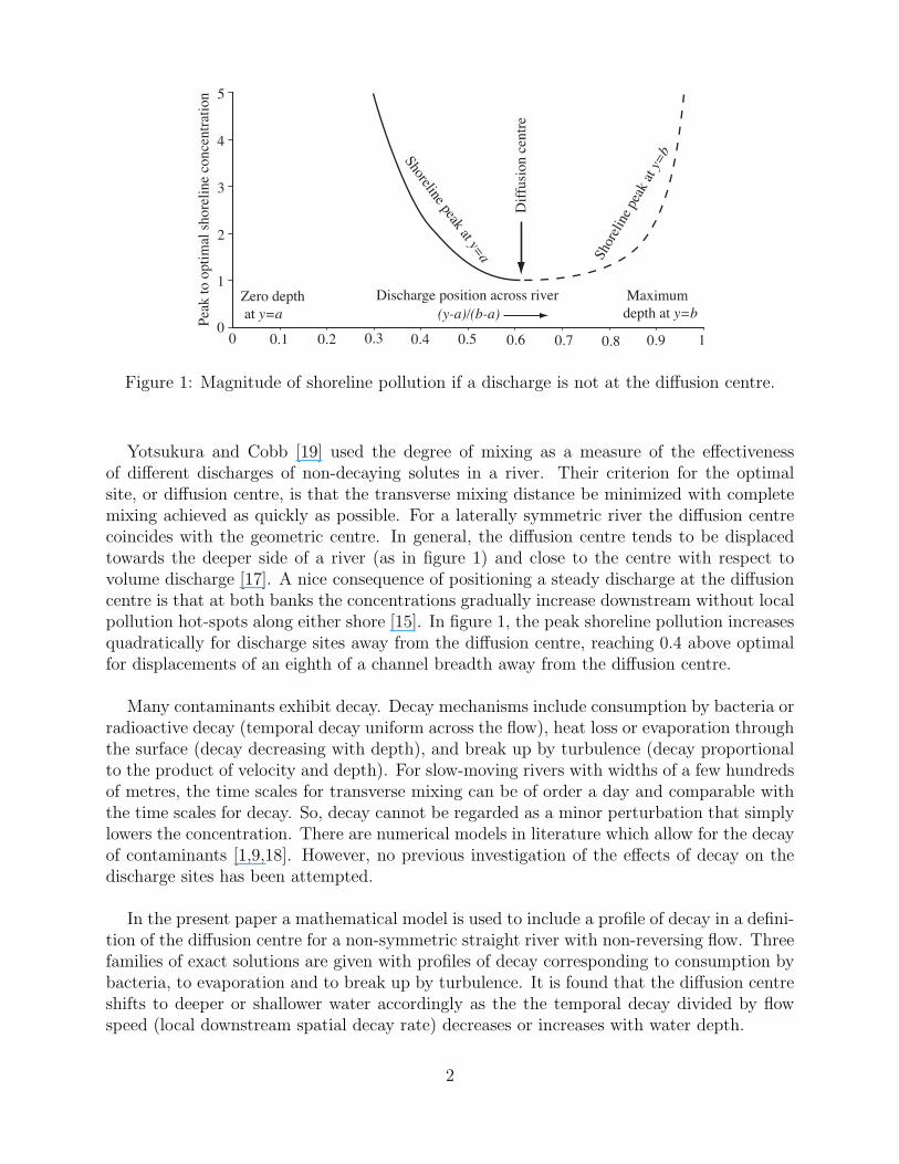
Effects of Contaminant Decay on the Diffusion Centre of a River P. Mebine * and R. Smith † Department of Mathematical Sciences, Loughborough University, LE11 3TU, United Kingdom Abstract Many contaminants exhibit decay (radioactive decay, consumed by bacteria, heat loss or evaporation through the surface, dissolution by turbulence). For a non-symmetric river with non-reversing flow, the effects of decay are allowed for in specifying the dif- fusion centre i.e. the optimal postion for a steady discharge. Three families of exact solutions are presented that illustrate the effect on the diffusion centre of cross-channel variation in the decay (uniform, decreasing or increasing with depth). The diffusion centre is shifted to deeper or to shallower water accordingly as the temporal decay divided by flow speed decreases or increases with water depth. Keywords: contaminant decay, diffusion centre, environmental impact, pollutant modes, variability of decay 1 Introduction Modern large-scale sewage works and industrial processes are designed to avoid intermittent high-level waste-water discharges, and instead are aimed at steady low-level discharges. The environmental impact can be further reduced by careful selection of the discharge location. In rivers, the near-shore or littoral zones contain more abundant plant, fish and animal communities than the main channel. A commonly advocated managerial policy to conserve these areas of economic importance is to choose the source location of large-scale contaminant discharges to avoid excessive shoreline concentrations. The magnitude of avoidable shoreline excesses is shown in figure 1 for the illustrative case of a conserved solute discharged at a steady rate from a single point into a channel with water depth that increases from zero at the left to maximum water depth at the right of figure 1. * Corresponding Author, E-mail: P. [email protected] † Prof. of Mathematics 1
-
Upload
unigerdeltawilberforceislandbayelsa -
Category
Documents
-
view
0 -
download
0
Transcript of Effects of Contaminant Decay on the Diffusion Centre of a River
Effects of Contaminant Decay on the Diffusion Centre ofa River
P. Mebine∗ and R. Smith†
Department of Mathematical Sciences, Loughborough University,LE11 3TU, United Kingdom
Abstract
Many contaminants exhibit decay (radioactive decay, consumed by bacteria, heatloss or evaporation through the surface, dissolution by turbulence). For a non-symmetricriver with non-reversing flow, the effects of decay are allowed for in specifying the dif-fusion centre i.e. the optimal postion for a steady discharge. Three families of exactsolutions are presented that illustrate the effect on the diffusion centre of cross-channelvariation in the decay (uniform, decreasing or increasing with depth). The diffusioncentre is shifted to deeper or to shallower water accordingly as the temporal decaydivided by flow speed decreases or increases with water depth.
Keywords: contaminant decay, diffusion centre, environmental impact, pollutant modes,variability of decay
1 Introduction
Modern large-scale sewage works and industrial processes are designed to avoid intermittenthigh-level waste-water discharges, and instead are aimed at steady low-level discharges. Theenvironmental impact can be further reduced by careful selection of the discharge location.In rivers, the near-shore or littoral zones contain more abundant plant, fish and animalcommunities than the main channel. A commonly advocated managerial policy to conservethese areas of economic importance is to choose the source location of large-scale contaminantdischarges to avoid excessive shoreline concentrations. The magnitude of avoidable shorelineexcesses is shown in figure 1 for the illustrative case of a conserved solute discharged at asteady rate from a single point into a channel with water depth that increases from zero atthe left to maximum water depth at the right of figure 1.
∗Corresponding Author, E-mail: P. [email protected]†Prof. of Mathematics
1
1
2
3
4
5
00.60.50.40.30.20.1 10.90.80.7
Pea
k t
o o
pti
mal
shore
line
conce
ntr
atio
n
(y-a)/(b-a)
Discharge position across river
Shoreline peak at y=a S
hore
line
pea
k at
y=b
Dif
fusi
on c
entr
e
0
Zero depth
at y=a
Maximum
depth at y=b
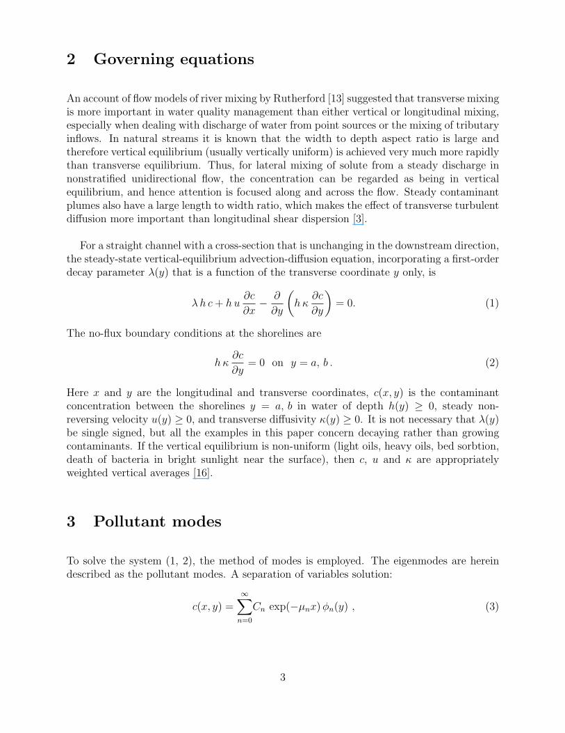
Figure 1: Magnitude of shoreline pollution if a discharge is not at the diffusion centre.
Yotsukura and Cobb [19] used the degree of mixing as a measure of the effectivenessof different discharges of non-decaying solutes in a river. Their criterion for the optimalsite, or diffusion centre, is that the transverse mixing distance be minimized with completemixing achieved as quickly as possible. For a laterally symmetric river the diffusion centrecoincides with the geometric centre. In general, the diffusion centre tends to be displacedtowards the deeper side of a river (as in figure 1) and close to the centre with respect tovolume discharge [17]. A nice consequence of positioning a steady discharge at the diffusioncentre is that at both banks the concentrations gradually increase downstream without localpollution hot-spots along either shore [15]. In figure 1, the peak shoreline pollution increasesquadratically for discharge sites away from the diffusion centre, reaching 0.4 above optimalfor displacements of an eighth of a channel breadth away from the diffusion centre.
Many contaminants exhibit decay. Decay mechanisms include consumption by bacteria orradioactive decay (temporal decay uniform across the flow), heat loss or evaporation throughthe surface (decay decreasing with depth), and break up by turbulence (decay proportionalto the product of velocity and depth). For slow-moving rivers with widths of a few hundredsof metres, the time scales for transverse mixing can be of order a day and comparable withthe time scales for decay. So, decay cannot be regarded as a minor perturbation that simplylowers the concentration. There are numerical models in literature which allow for the decayof contaminants [1,9,18]. However, no previous investigation of the effects of decay on thedischarge sites has been attempted.
In the present paper a mathematical model is used to include a profile of decay in a defini-tion of the diffusion centre for a non-symmetric straight river with non-reversing flow. Threefamilies of exact solutions are given with profiles of decay corresponding to consumption bybacteria, to evaporation and to break up by turbulence. It is found that the diffusion centreshifts to deeper or shallower water accordingly as the the temporal decay divided by flowspeed (local downstream spatial decay rate) decreases or increases with water depth.
2
2 Governing equations
An account of flow models of river mixing by Rutherford [13] suggested that transverse mixingis more important in water quality management than either vertical or longitudinal mixing,especially when dealing with discharge of water from point sources or the mixing of tributaryinflows. In natural streams it is known that the width to depth aspect ratio is large andtherefore vertical equilibrium (usually vertically uniform) is achieved very much more rapidlythan transverse equilibrium. Thus, for lateral mixing of solute from a steady discharge innonstratified unidirectional flow, the concentration can be regarded as being in verticalequilibrium, and hence attention is focused along and across the flow. Steady contaminantplumes also have a large length to width ratio, which makes the effect of transverse turbulentdiffusion more important than longitudinal shear dispersion [3].
For a straight channel with a cross-section that is unchanging in the downstream direction,the steady-state vertical-equilibrium advection-diffusion equation, incorporating a first-orderdecay parameter λ(y) that is a function of the transverse coordinate y only, is
λ h c + hu∂c
∂x− ∂
∂y
(hκ
∂c
∂y
)= 0. (1)
The no-flux boundary conditions at the shorelines are
hκ∂c
∂y= 0 on y = a, b . (2)
Here x and y are the longitudinal and transverse coordinates, c(x, y) is the contaminantconcentration between the shorelines y = a, b in water of depth h(y) ≥ 0, steady non-reversing velocity u(y) ≥ 0, and transverse diffusivity κ(y) ≥ 0. It is not necessary that λ(y)be single signed, but all the examples in this paper concern decaying rather than growingcontaminants. If the vertical equilibrium is non-uniform (light oils, heavy oils, bed sorbtion,death of bacteria in bright sunlight near the surface), then c, u and κ are appropriatelyweighted vertical averages [16].
3 Pollutant modes
To solve the system (1, 2), the method of modes is employed. The eigenmodes are hereindescribed as the pollutant modes. A separation of variables solution:
c(x, y) =∞∑
n=0
Cn exp(−µnx) φn(y) , (3)
3
leads to the introduction of the pollutant modes φn(y) and their associated spatial decayrates (eigenvalues) µn:
d
dy
(hκ
dφn
dy
)+ [µn u− λ] hφn = 0 , (4)
with
hκdφn
dy= 0 on y = a, b . (5)
Modes are only known explicitly for restricted families of exactly solvable test cases, butexist and are countable for any non-negative depth, diffusivity and velocity profiles.
It is conventional to order the modes in increasing values of the spatial decay rates
µ0 < µ1 < µ2 < . . . . (6)
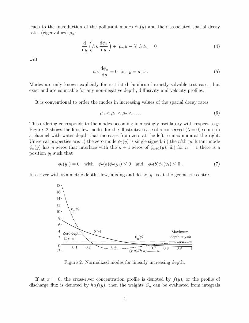
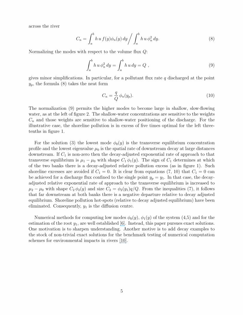
This ordering corresponds to the modes becoming increasingly oscillatory with respect to y.Figure 2 shows the first few modes for the illustrative case of a conserved (λ = 0) solute ina channel with water depth that increases from zero at the left to maximum at the right.Universal properties are: i) the zero mode φ0(y) is single signed; ii) the n’th pollutant modeφn(y) has n zeros that interlace with the n + 1 zeros of φn+1(y); iii) for n = 1 there is aposition y1 such that
φ1(y1) = 0 with φ2(a)φ2(y1) ≤ 0 and φ2(b)φ2(y1) ≤ 0 . (7)
In a river with symmetric depth, flow, mixing and decay, y1 is at the geometric centre.
-2
0
2
4
6
8
10
12
14
16
18
10.90.80.70.40.20.1(y-a)/(b-a)
Maximum
depth at y=bZero depth
at y=a
φ2(y)
φ1(y)
φ0(y)
Figure 2: Normalized modes for linearly increasing depth.
If at x = 0, the cross-river concentration profile is denoted by f(y), or the profile ofdischarge flux is denoted by huf(y), then the weights Cn can be evaluated from integrals
4
across the river
Cn =
∫ b
a
hu f(y)φn(y) dy
/∫ b
a
hu φ2n dy. (8)
Normalizing the modes with respect to the volume flux Q:∫ b
a
hu φ2n dy =
∫ b
a
hu dy = Q , (9)
gives minor simplifications. In particular, for a pollutant flux rate q discharged at the pointyp, the formula (8) takes the neat form
Cn =q
Qφn(yp). (10)
The normalization (9) permits the higher modes to become large in shallow, slow-flowingwater, as at the left of figure 2. The shallow-water concentrations are sensitive to the weightsCn and those weights are sensitive to shallow-water positioning of the discharge. For theillustrative case, the shoreline pollution is in excess of five times optimal for the left three-tenths in figure 1.
For the solution (3) the lowest mode φ0(y) is the transverse equilibrium concentrationprofile and the lowest eigenvalue µ0 is the spatial rate of downstream decay at large distancesdownstream. If C1 is non-zero then the decay-adjusted exponential rate of approach to thattransverse equilibrium is µ1 − µ0 with shape C1 φ1(y). The sign of C1 determines at whichof the two banks there is a decay-adjusted relative pollution excess (as in figure 1). Suchshoreline excesses are avoided if C1 = 0. It is clear from equations (7, 10) that C1 = 0 canbe achieved for a discharge flux confined to the single point yp = y1. In that case, the decay-adjusted relative exponential rate of approach to the transverse equilibrium is increased toµ2 − µ0 with shape C2 φ2(y) and size C2 = φ2(y1)q/Q. From the inequalities (7), it followsthat far downstream at both banks there is a negative departure relative to decay adjustedequilibrium. Shoreline pollution hot-spots (relative to decay adjusted equilibrium) have beeneliminated. Consequently, y1 is the diffusion centre.
Numerical methods for computing low modes φ0(y), φ1(y) of the system (4,5) and for theestimation of the root y1, are well established [6]. Instead, this paper pursues exact solutions.One motivation is to sharpen understanding. Another motive is to add decay examples tothe stock of non-trivial exact solutions for the benchmark testing of numerical computationschemes for environmental impacts in rivers [10].
5
4 Flow parameters in straight channels
Flows in natural streams tend to be turbulent. Elder [3] showed that the local turbulentdiffusivities are proportional to the product of the local water depth and longitudinal velocity.This implies [8,13,14], that the longitudinal velocity varies as square-root of the depth andthe diffusivity as the three-halves power of the water depth:
u = U
(h
H
) 12
, κ = K
(h
H
) 32
. (11)
The capital letters H, U and K denote the depth, flow and transverse mixing at a referenceposition in the channel. The depth-linked formulae (11) ensure that in the deepest parts ofthe channel the velocity is greatest and transverse mixing is most vigorous [2]. It is implicitthat the pollutant is sufficiently dilute that it does not significantly modify the turbulence(e.g. applicable to oil in droplets but not to a continuous oil slick).
The illustrative examples in this paper use power-law models for the decay:
λ = Λ
(h
H
)δ+ 12
. (12)
For positive (or negative) δ the ratio λ(y)/u(y) increases (or decreases) with depth.
With the representations (11, 12) the eigenvalue problem (4, 5) becomes
Kd
dy
((h
H
) 52 dφn
dy
)+
(h
H
) 32
[µn U − Λ
(h
H
)δ]
φn = 0 , (13)
with (h
H
) 52 dφn
dy= 0 on y = a, b . (14)
For zero decay, the concept of the diffusion centre and the method of modes that is usedto identify it, are not restricted to straight non-varying channels [15]. The mathematicslooks more daunting because of the need to use of flow-following coordinates [20]. Also, themodes split into downstream evolving φn(x, y) and upstream evolving φ̂n(x, y) adjoints. Thediffusion centre is where φ̂1(x, y1(x)) = 0. It is evolving upstream in response to downstreamchanges to the cross-sectional profile on the length scale 1/µ2 of cross-sectional mixing [15]i.e. it is downstream of the discharge where shoreline pollution excesses might otherwisehave occured. With decay, the principal changes would be that the transverse equilibriumφ0(x, y) ceases to be constant across the channel and has decay µ0(x) along the flow.
6
5 Linearly increasing depth
For illustrative purposes, the chosen depth profile across the flow is linear increase from zerodepth at one side y = 0 to maximum depth H at the other side y = B:
h(y) = H( y
B
)for 0 < y < B. (15)
Decay proportional to the flow speed λ = Λ(h/H)12 (i.e. δ = 0) has no effect on the
modes. The modes are unchanged from those for a conserved solute. The lowest mode isconstant across the channel φ0 = 1. Higher modes (normalized) can be represented [15]:
φn =
(an(y/B)
12
)−1
sin(an(y/B)
12
)− cos
(an(y/B)
12
)(y/B) (5
2)
12
{1 + cos(an) sin(an)
an− 2 sin(an)2
a2n
} 12
. (16)
The square-root terms in the denominator that normalize the modes for arbitrary an.
The no-flux boundary condition (14) at y = B restricts the an to being non-negative rootsof the equation:
sin(an) = −3 an cos(an)
a2n − 3
, a1 = 5.763 , a2 = 9.095 , an ≈ nπ − 3
n π. (17)
The construction of figure 1 from the modal solution (3) used up to 40 modes to achievehigh accuracy. Figure 2 shows the n = 0, 1, 2 normalized modes. The diffusion centre is at
y1/B = 0.608 . (18)
Decay proportional to the flow speed, augments the eigenvalues µn by Λ/U :
µn =K a2
n
4 U B2+
Λ
U. (19)
For n = 2, transverse mixing and decay give equal contributions to µn for ΛB2/K ≈ 20.For larger rates of decay shoreline pollution becomes insignificant unless the discharge isirresponsibly close to shore. The subsequent computations are restricted to ΛB2/K ≤ 10.
In the context of pollution minimisation from sudden discharges of pollutants, Daish [2]used piecewise linear depth profiles to construct a wide range of test problems. The followingthree sub-sections concern the linear depth profile (15), but with decay profiles correspondingto uniform consumption by bacteria, to evaporation and to break up by turbulence. Thediffusion centre y1 is found to deviate by ±B/8 from the non-decaying reference case (18).
7
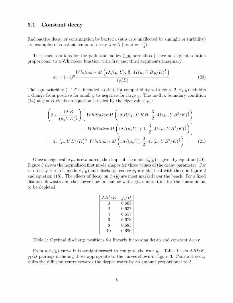
5.1 Constant decay
Radioactive decay or consumption by bacteria (at a rate unaffected by sunlight or turbidity)are examples of constant temporal decay λ = Λ (i.e. δ = −1
2) .
The exact solutions for the pollutant modes (not normalised) have an explicit solutionproportional to a Whittaker function with first and third arguments imaginary:
φn = (−1)nWhittaker M
(i Λ/(µnU), 3
2, 4 i (µn U B y/K)
12
)(y/B)
. (20)
The sign switching (−1)n is included so that, for compatibility with figure 2, φ1(y) exhibitsa change from positive for small y to negative for large y. The no-flux boundary condition(14) at y = B yields an equation satisfied by the eigenvalues µn:(
2 +i Λ B
(µnU K)12
)[Whittaker M
(i Λ B/(µnU K)
12 ,
3
2, 4 i (µn U B2/K)
12
)− Whittaker M
(i Λ/(µnU) + 1,
3
2, 4 i (µn U B2/K)
12
)]= 2 i
(µn U B2/K
) 12 Whittaker M
(i Λ/(µnU),
3
2, 4 i (µn U B2/K)
12
). (21)
Once an eigenvalue µn is evaluated, the shape of the mode φn(y) is given by equation (20).Figure 3 shows the normalized first mode shapes for three values of the decay parameter. Forzero decay the first mode φ1(y) and discharge centre y1 are identical with those in figure 2and equation (18). The effects of decay on φ1(y) are most marked near the beach. For a fixeddistance downstream, the slower flow in shallow water gives more time for the contaminantto be depleted.
ΛB2/K y1/B0 0.6082 0.6374 0.6576 0.6738 0.685
10 0.696
Table 1: Optimal discharge positions for linearly increasing depth and constant decay.
From a φ1(y) curve it is straightforward to compute the root y1. Table 1 lists ΛB2/K,y1/B pairings including those appropriate to the curves shown in figure 3. Constant decayshifts the diffusion centre towards the deeper water by an amount proportional to Λ.
8

ΛΒ /Κ=8
2
ΛΒ
/Κ=0
2
−1
0
1
2
3
4
5
6
7
10.90.80.7
0.60.50.40.30.20.1
y/B
ΛΒ /Κ=42
Zero depth
at y=0
Maximum
depth at y=B
Figure 3: First mode φ1(y) for constant decay Λ and linearly increasing depth.
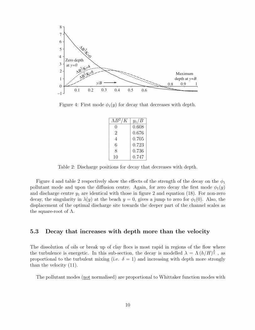
5.2 Decay that decreases with depth
The decay can decrease with depth if c(y, t) is a number count of bacteria which are killed bysunlight [7] only in the top few metres of the water column. A second example is removal atthe bed (feeding by marine micro-organisms, fungi or yeasts). A third example is air-watercontaminant exchange at the surface. For example, evaporation accounts for largest loss inoil volume during the early stages [11,12]. Fingas [4,5] notes that light crude oils can lose asmuch as 75 per cent of their original volume within the first few days after a spill; medium-weight crudes might lose as much as 40 per cent of the original volume. Heavy crude orresidual oils, on the hand, will probably only lose about 10 per cent of their volume in thefirst few days.
An exactly solvable model problem that illustrates decay decreasing with depth is λ =Λ(h/H)−
12 (i.e. δ = −1) . The modes (not normalised) are proportional to a Bessel function
of non-integer-order:
φn =Bessel J
((9
4+ 4 Λ B2/K)
12 , 2 (µn U B y/K)
12
)(y/B)
34
. (22)
The no-flux boundary condition (14) at y = B yields the eigenvalue equation with roots µn:
(9
4+ 4 Λ B2/K)
12 Bessel J
((9
4+ 4 Λ B2/K)
12 , 2 (µn U B y/K)
12
)−2 (µn U B2/K)
12 Bessel J
((9
4+ 4 Λ B2/K)
12 + 1, 2 (µn U B2/K)
12
)=
3
2Bessel J
((9
4+ 4 Λ B2/K)
12 , 2 (µn U B2/K)
12
). (23)
9
ΛΒ /Κ=8
2
ΛΒ /Κ
=0
2
−1
0
1
2
3
4
5
6
7
10.90.8
0.60.50.40.30.20.1
y/B
ΛΒ /Κ=4
2
8
Maximum
depth at y=B
Zero depth
at y=0
Figure 4: First mode φ1(y) for decay that decreases with depth.
ΛB2/K y1/B0 0.6082 0.6764 0.7056 0.7238 0.736
10 0.747
Table 2: Discharge positions for decay that decreases with depth.
Figure 4 and table 2 respectively show the effects of the strength of the decay on the φ1
pollutant mode and upon the diffusion centre. Again, for zero decay the first mode φ1(y)and discharge centre y1 are identical with those in figure 2 and equation (18). For non-zerodecay, the singularity in λ(y) at the beach y = 0, gives a jump to zero for φ1(0). Also, thedisplacement of the optimal discharge site towards the deeper part of the channel scales asthe square-root of Λ.
5.3 Decay that increases with depth more than the velocity
The dissolution of oils or break up of clay flocs is most rapid in regions of the flow wherethe turbulence is energetic. In this sub-section, the decay is modelled λ = Λ (h/H)
32 , as
proportional to the turbulent mixing (i.e. δ = 1) and increasing with depth more stronglythan the velocity (11).
The pollutant modes (not normalised) are proportional to Whittaker function modes with
10

all three arguments real:
φn =Whittaker M(1
2µn U B/(Λ K)
12 , 3
4, 2(Λ/K)
12 y)
(y/B)54
. (24)
The no-flux boundary condition at y = B yields an equation satisfied by the eigenvalues µn:(5
4+
µn U B
2 (Λ K)12
) [Whittaker M
(1
2µn U B/(Λ K)
12 ,
3
4, 2(Λ/K)
12 B
)− Whittaker M(
1
2µn U B/(Λ K)
12 + 1,
3
4, 2(Λ/K)
12 B)
]= (Λ/K)
12 B Whittaker M(
1
2µn U B/(Λ K)
12 ,
3
4, 2(Λ/K)
12 B) . (25)
10.90.80.7
0.60.50.40.30.20.1
y/B
ΛΒ
/Κ=8
2
ΛΒ /Κ
=0
2
−1
0
1
2
3
4
5
6
7
8
9
10
Zero depth
at y=0
Maximum
depth at y=B
Figure 5: First mode φ1(y) for decay that increases with depth.
ΛB2/K y1/B0 0.6082 0.5894 0.5686 0.5448 0.518
10 0.489
Table 3: Discharge positions for decay that increases with depth.
Figure 5 and table 3 respectively show the first pollutant mode φ1(y) and the optimumdischarge site y1 for a few values of ΛB2/K. Once more, for zero decay the first mode φ1(y)and discharge centre y1 are identical with those in figure 2 and equation (18). Contrary tothe previous two sub-sections, the diffusion centre shifts to the shallower water.
11
6 Ratio λ/u as an indicator for changes in y1
A physical interpretation of the ratio λ(y)/u(y) is as the local spatial decay rate for thecontaminant at the cross-channel location y. For the special case of linear depth, it wasobserved in §5 that if λ(y)/u(y) is constant (i.e. δ = 0), then the modal shapes φn(y) arenot effected by decay and the spatial decay rates µn for the modes are merely augmentedby that constant spatial decay rate λ/u. It is evident from the square-bracketed terms inequation (4), that the same is true whatever the depth profile h(y).
It is natural to investigate whether the depth-dependence of the ratio λ(y)/u(y), or thesign and magnitude of the exponent δ in the power-law model (12), can be used as anindicator for changes to the position of the diffusion centre. In §5.1 and figure (3), λ(y)/u(y)decreases with negative exponent δ = −1
2and the diffusion centre shifts weakly to deeper
water. In §5.2 and figure (4), λ(y)/u(y) decreases more strongly with negative exponentδ = −1 and the diffusion centre shifts more strongly to deeper water. Finally, in §5.3 andfigure (5), λ(y)/u(y) increases with positive exponent δ = 1 and the diffusion centre shiftsto shallower water. Hence, the diffusion centre is shifted to deeper or to shallower wateraccordingly as the ratio λ(y)/u(y) decreases or increases with water depth (i.e. δ negativeor positive).
7 Concluding remarks
Avoidable shoreline pollution excesses can be large for steady discharges close to shore. Thespecial cases solved in this paper sharpen insight about how loss mechanisms displace thebest siting of steady discharges away from the site appropriate to non-decaying solutes. Themixing or diffusion centre is shifted to deeper or to shallower water accordingly as the spatialdecay rate (i.e. ratio λ(y)/u(y)) decreases or increases with water depth.
The three families of exact modes (20, 22, 24) together with the exact series solution (3)and weights (8) permit the construction of exact solutions that include decay. Such exactsolutions extend the scope for for the benchmark testing [10] of numerical computationschemes for environmental impacts in rivers.
Commonly, a steady discharge will comprise a mixture of pollutants with different decayprocesses and rates. The chosen discharge site will be a compromise between the diffusioncentre for the constituent pollutants. For the wide range of cases considered in this paper,the optimal discharge position for the different decay processes is never found to be morethan one eighth of a channel breadth from the site appropriate to non-decaying solutes.For each decaying constituent the displacement between the discharge site and the diffusioncentre for that constituent, corresponds to shoreline pollution excesses less than a factor of0.4 above optimal (as contrasted to the factor of 4.0 excess at which figure 1 is truncated).
12
The variety of exact solutions in this paper illustrate the robustness of the commonsensepolicy that, to avoid large shoreline pollution excesses from any of the constituents in amixture of pollutants, the discharge should be sited more or less in the middle of the river.
Acknowledgements
We thank the referees for constructive comments. The first author would like to thankBayelsa State Government of Nigeria for financial support through the award of a PhDresearch fellowship.
References
1. Bikangaga, J. H. and Nassehi, V.: 1995, Application of Computer Modelling Tech-inques to the Determination of Optimum Efluent Discharge Policies in Tidal WaterSystems. Wat. Res.,29,10, 2367-2375.
2. Daish, N. C.: 1985, The Optimal discharge profiles for sudden contaminant releases insteady, unform open-channel flow. J. Fluid Mech., 159, 303-321.
3. Elder, J. W.: 1959, The dispersion of marked fluid in turbulent shear flow. J. FluidMech., 5, 544-560.
4. Fingas, M.: 1994a, Studies on the evaporation of oil spills. Seventeenth Arctic MarineOil Spill Program (AMOP) Tecnical Seminar, Vancouver, Canada, June 8-10, 1994,Vancouver, British Columbia: Environment Canada, 189-210.
5. Fingas, M.: 1985, A literature review of the physics and predictive modelling of oilspill evaporation. Journal of Hazardous Materials, 42,157-175.
6. Fox, L.: 1957, The numerical solution of two-point boundary value problems, OxfordUniversity Press, London UK.
7. Gould, D.J. and Munro, D.: 1981, Relevance of Microbial Mortality to outfall Design.Coastal Discharges, Thomas Telford, London, U.K., 45-50.
8. Kay, A.: 1987, The Effect of Cross-Stream Depth Variations upon Contaminant Dis-persion in a Vertically Well-mixed Current. Estuarine, Coastal and Shelf Science, 24,177-204.
9. Nassehi, V. and Bikangaga, J. H.: 1993, A mathematical model for the hydrodynamicsand pollutants transport in long and narrow tidal rivers. Appl. Math. Modelling, 17,415-422.
13
10. Nassehi, V. and Passone, S.: 2005, Testing Accuracy of Finite Element and RandomWalk Schemes in Prediction of Pollutant Dispersion in Coastal Waters. EnvironmentalFluid Mech., to appear.
11. Overstreet, R. and Galt, J.A.: 1995, Physical Processes Affecting the Movementand Spresding of Oils in Inland Waters. NOAA/Hazardous Materials Response andAsssessment Division Seattle, Washingto, HAZMAT Report 95-7.
12. Reddy, G.S. and Brunet, M.: 2003, Numerical Prediction of Oil Slick Movement inGabes Estuary, www.fluidyn.com/Research.
13. Rutherford, J. C.: 1994, River Mixing, Wiley, Chichester UK.
14. Smith, R.: 1981, Effect of non-uniform currents and depths variations upon steadydischarges in shallow water. J. Fluid Mech., 110, 373-380.
15. Smith, R.: 1982, Where to put a steady discharge in a river. J. Fluid Mech., 115, 1-11.
16. Smith, R.: 1996, Horizontal fractionation of rising and sinking particles in wind-affectedcurrents. J. FLuid Mech.., 316, 325-334.
17. Smith, R.: 2004, Mixing Center of a Channel. J. Hydraulic Engineering, 130, 2,165-169.
18. Yoo, M. K., Cho, S. W., and Jun, K. S.: 2003, Unsteady Dispersion of NonconservativePollutants in Natural Rivers. www.kfki.baw.de/conferences.
19. Yotsukura, N. and Cobb, E. D.: 1972, Transverse diffusion of solutions in naturalstreams. U. S. Geo. Survey Paper, no.582 C.
20. Yotsukura, N. and Sayre, W.W.: 1976, Transverse mixing in natural channels. U. S.Geo. Survey Paper, no.582 C.
14