water

Article

Numerical Analysis of Recharge Rates andContaminant Travel Time in LayeredUnsaturated Soils

Adam Szymkiewicz 1,*, Julien Savard 2,3 and Beata Jaworska-Szulc 1

1 Faculty of Civil and Environmental Engineering, Gdansk University of Technology, ul. Narutowicza 11/12,80-233 Gdansk, Poland; bejaw@pg.edu.pl

2 Conservatoire National des Arts et Métiers ChampagneArdenne, CEDEX 03, F-75141 Paris, France;jsavard@laposte.net

3 Nancy Agency, SociétéAuxiliaire de Distribution de l’Eau-CompagnieGénérale desTravauxHydrauliques (SADE-CGTH), 54220 Malzéville, France

* Correspondence: adams@pg.edu.pl; Tel.: +48-58-347-1085

Received: 12 February 2019; Accepted: 12 March 2019; Published: 16 March 2019�����������������

Abstract: This study focused on the estimation of groundwater recharge rates and travel time ofconservative contaminants between ground surface and aquifer. Numerical simulations of transientwater flow and solute transport were performed using the SWAP computer program for 10 layeredsoil profiles, composed of materials ranging from gravel to clay. In particular, sensitivity of the resultsto the thickness and position of weakly permeable soil layers was carried out. Daily weather dataset from Gdansk (northern Poland) was used as the boundary condition. Two types of cover wereconsidered, bare soil and grass, simulated with dynamic growth model. The results obtained withunsteady flow and transport model were compared with simpler methods for travel time estimation,based on the assumptions of steady flow and purely advective transport. The simplified methodswere in reasonably good agreement with the transient modelling approach for coarse textured soilsbut tended to overestimate the travel time if a layer of fine textured soil was present near the surface.Thus, care should be taken when using the simplified methods to estimate vadose zone travel timeand vulnerability of the underlying aquifers.

Keywords: unsaturated zone; Richards equation; contaminant transport; time lag;heterogeneous soils

1. Introduction

In view of the increasing use of groundwater resources worldwide, there is a need to developefficient methods to quantify the recharge rate (i.e., the amount of water from precipitation reachingthe groundwater table) and the time of migration of contaminants from the ground surface to thegroundwater table. These two tasks are closely related, since they both require knowledge of watervelocity in the vadose zone, which is generally variable in space and time. In order to achieve this goal,numerical models of unsaturated flow and transport are often used [1–12]. They can be considered asan approach alternative or complementary to other, more costly and time-consuming methods (e.g.,lysimeters, tracer experiments). Several computer codes can be used for this purpose, some of themfreely available, for example, HYDRUS-1D [13], SWAP [14], UNSAT-H [15], HELP [16]. There is also agrowing body of literature and online resources from which the input data for numerical simulationscan be obtained, including parameters of soil water retention, permeability, root water uptake anddetailed weather data. Nevertheless, the widespread use of numerical modelling is still hampered bythe limited availability of realistic data for specific scenarios, need for the user expertise, relatively

Water 2019, 11, 545; doi:10.3390/w11030545 www.mdpi.com/journal/water

Water 2019, 11, 545 2 of 13

long times of computation and possible convergence problems in transient flow simulations. For thisreason, simplified approaches to quantify recharge and contaminant travel time remain a useful tool inhydrogeological practice [17–20].

Simplified methods of travel time estimation are usually based on the assumption of uniformsteady vertical water flow through the vadose zone, corresponding to the average recharge rate.Only transport by advection is considered and the advective velocity is obtained by dividing therecharge rate by the mobile water content (often assumed equal to the total water content). In thesimplest approach, the water content is assumed constant within each soil layer constituting thevertical profile. More detailed methods consider variability of the water content in each material layer.The purely advective transport model is considered to provide a safe estimate of the arrival time ofcontaminant at the groundwater table, due to neglecting adsorption and other processed causingdegradation and retardation of the dissolved substance. However, the arrival time may be substantiallyshorter if the hydrodynamic dispersion processes are taken into account [21].

Sousa et al. [19] investigated the performance of three methods based on steady flow assumptionfor 8 layered soil profiles on a site near Woodstock, Ontario, Canada. They solved numerically theequation describing steady unsaturated water flow, in order to obtain a detailed distribution of thewater content in each profile. This method was considered as the most accurate in the context oftheir study. Additionally, Sousa et al. [19] estimated the travel time with two other approaches: usinghydrostatic profile of the water content above the groundwater table and using constant average valuesof the mobile water content in each soil layer. The recharge rates were estimated from earlier tracerexperiments. Significant differences were observed in the values of travel time obtained with variousmethods. However, no attempt was undertaken to compare them with simulations of unsteady flowand transport driven by time-variable fluxes at the soil surface.

More recently, Szymkiewicz et al. [21] carried out a comparison between transient and steady-statebased methods for estimating time lag for soil profiles with and without root zone. They showedthat even if the average recharge rate obtained from transient simulations is used as the input in thesteady state methods, the resulting travel times vary considerably. None of the simple methods wasable to match the transient simulation results for all scenarios, although the agreement was betterfor a coarse textured soil (sand) than for a fine textured soil (clay loam). However, in Reference [21]only homogeneous soil profiles were considered. Moreover, the root water uptake was modelled ina simplified manner. In the scenarios with vegetation it was assumed that there is no evaporationfrom the soil surface and the total amount of potential evapotranspiration was assigned as a sinkterm to the root zone, regardless of the season of the year. For a more realistic result, the potentialevapotranspiration should be split between the evaporation from the soil surface and the transpirationby roots, depending on the stage of plant growth. In the current study we extended our previousanalysis by taking into account: (i) layered structure of soil profiles and (ii) a more detailed modelof vegetation cover, including variable-in-time split between evaporation and transpiration. For thispurpose, we used SWAP numerical code, which contains a detailed module for grass growth andtranspiration [14]. We considered 2 homogeneous and 8 layered soil profiles. The recharge rate wasmostly affected by the texture of the top soil layer. The travel time was more sensitive to the thicknessof soil layers than to their position in the profile (except for the top layer). The presence of root zonesignificantly decreased recharge and increased travel time, although to a less extent than in our earlierstudy. The methods based on steady flow assumption gave results relatively close to the transientsimulations for coarse textured soils but tended to overestimate the travel time in fine textured soils,in agreement with our previous findings [21].

Water 2019, 11, 545 3 of 13

2. Materials and Methods

2.1. General Assumptions

Following the state-of-the-art approach, for example, [7], we assume that the water flowis described by the Richards Equation (1) and the solute transport by an advection-dispersionEquation (2):

∂θ(h)∂t

+∂q∂z

+ S(h) = 0, q = −k(θ(h))(

∂h∂z

+ 1)

, (1)

∂(θc)∂t

=∂

∂z

(θD

∂c∂z

)− ∂(qc)

∂z, (2)

where: t—time, z—vertical coordinate (oriented upwards), h—soil water pressure head (negativein the unsaturated zone), θ—volumetric water content, q—volumetric water flux (Darcy velocity),S(h)—function representing water uptake by plant roots, k—hydraulic conductivity, c—soluteconcentration, D—hydrodynamic dispersion coefficient.

The root water uptake function S(h) was computed according to the model of Feddes et al. [22],with additional compensation term, as described in Reference [14]. Reduction factors due to oxygenstress and drought stress were included.

The dispersion coefficient depends only on the mechanical dispersion (molecular diffusion isneglected): D = a|q| + Dm*, where a is the longitudinal dispersivity. A constant value of a = 6cm wasused in all simulations. This value corresponds to 0.01 of the length scale of profiles A-F describedbelow. We chose it in line with our previous simulations described in Reference [21], in order tominimize the influence of dispersion on the solute travel time and facilitate comparison with simplifiedmethods, which take into account only advection. As shown in Reference [21], larger values ofdispersivity (e.g., equal to 0.1 profile depth [5]) lead to significantly earlier occurrence of the solute atthe groundwater table. The dependence of dispersivity on the length scale is often associated withlocal scale variability of soil hydraulic parameters and the presence of heterogeneity patterns morecomplex than the simple structure of horizontal layers considered here. Similarly, preferential flowand transport phenomena and dual-porosity/dual-permeability behaviour, described for example inReferences [23,24], are not considered in this work. The present analysis is limited to one-dimensionalsetting and thus does not take into account the possibility of horizontal flow within soil layers andalong layer interfaces, which may affect the recharge rate and contaminant travel time.

2.2. Structure and Hydraulic Properties of Soils

Calculations were performed for 10 soil profiles, as shown in Figure 1. In the first group of profiles(Figure 1A–G) the depth to groundwater table was set to 6m. The homogeneous sand and clay profiles(A and B) were considered as baseline cases. Profiles C and D represent simple layered structures withhalf of the profile occupied by each soil type. Profiles E–G contain a thin clay layer in sand material,positioned at different depths. This kind of structure has been encountered on glacial outwash plainin the region of Tuchola (northern Poland). Profile H can be considered typical for glacial moraineuplands in the region of Puck (northern Poland), where a confined aquifer is overlaid by multiplelayers of glacial till deposits. Finally, profiles I and J are taken from [19] (respectively profiles 1 and6 in the original paper). All soil materials are characterized by the van Genuchte-Mualem hydraulicfunctions [25]:

Se =θ − θr

θs − θr=[1 + (α|h|)ng

]−mg , k = kskr = ks√

Se

[1−

(1− S

1/mge

)mg]2

(3)

where Se—effective (normalized) water saturation, θr—residual water content, θs—water contentat fully saturated (or field saturated) conditions, α—parameter related to the air entry pressure(depending on the size of pores), ng, mg parameters related to the pore size distribution (mg = 1 − 1/ng),

Water 2019, 11, 545 4 of 13

ks—hydraulic conductivity at saturation, kr—relative hydraulic conductivity. Parameters of each soilmaterial are listed in Table 1. Soils in profiles A–H are characterized by average parameters for theirtextural classes, as reported in Reference [26]. For profiles I and J we used the parameters from theoriginal study [19].Water 2019, 11, x FOR PEER REVIEW 4 of 13

Figure 1. Soil profiles used in numerical simulations.

Table 1. Parameters of the soil materials.

Soil Type θr (-)

θs (-)

α (m−1)

ng (-)

ks (m s−1)

θfield Range (-)

Sand [25] 0.045 0.430 14.50 2.68 8.25 × 10−5 0.07−0.10 Silty clay [25] 0.07 0.36 0.50 1.09 5.56 × 10−8 0.24−0.38

Sandy loam [25] 0.065 0.41 7.50 1.89 1.22 × 10−5 0.18−0.26 Loam [25] 0.078 0.43 3.60 1.56 2.89 × 10−6 0.24−0.38

Loamy sand [25] 0.057 0.41 12.40 2.28 4.05 × 10−5 0.18−0.26 Silt [19] 0.021 0.43 0.66 1.68 8.00 × 10−8 0.30−0.36

Gravelly silt [19] 0.016 0.41 2.67 1.45 1.00 × 10−6 0.18−0.36 Gravel [19] 0.001 0.28 49.30 2.19 5.00 × 10−2 0.05−0.10

Clayey sand [19] 0.020 0.40 3.48 1.75 5.00 × 10−5 0.18−0.26 Medium sand [19] 0.019 0.36 3.52 3.18 5.00 × 10−3 0.07−0.10

Silty sand [19] 0.018 0.37 3.48 1.75 5.00 × 10−4 0.18−0.26

2.3. Initial and Boundary Conditions

Water flow in vadose zone is driven by precipitation and evaporation fluxes and detailed weather data are necessary to carry out transient analysis. For all profiles we used daily data recorded at the weather station of the Gdańsk University of Technology (Poland) in the period 2011–2015. The average annual precipitation was 550 mm/year. For bare soil scenarios the potential evaporation was calculated by the SWAP code using the Penman-Monteith method, based on the provided values of temperatures, wind speed, relative humidity and solar radiation and the bare soil

Figure 1. Soil profiles used in numerical simulations.

Table 1. Parameters of the soil materials.

Soil Type θr(-)

θs(-)

α(m−1)

ng(-)

ks(m s−1)

θfield Range(-)

Sand [25] 0.045 0.430 14.50 2.68 8.25 × 10−5 0.07−0.10Silty clay [25] 0.07 0.36 0.50 1.09 5.56 × 10−8 0.24−0.38

Sandy loam [25] 0.065 0.41 7.50 1.89 1.22 × 10−5 0.18−0.26Loam [25] 0.078 0.43 3.60 1.56 2.89 × 10−6 0.24−0.38

Loamy sand [25] 0.057 0.41 12.40 2.28 4.05 × 10−5 0.18−0.26Silt [19] 0.021 0.43 0.66 1.68 8.00 × 10−8 0.30−0.36

Gravelly silt [19] 0.016 0.41 2.67 1.45 1.00 × 10−6 0.18−0.36Gravel [19] 0.001 0.28 49.30 2.19 5.00 × 10−2 0.05−0.10

Clayey sand [19] 0.020 0.40 3.48 1.75 5.00 × 10−5 0.18−0.26Medium sand [19] 0.019 0.36 3.52 3.18 5.00 × 10−3 0.07−0.10

Silty sand [19] 0.018 0.37 3.48 1.75 5.00 × 10−4 0.18−0.26

2.3. Initial and Boundary Conditions

Water flow in vadose zone is driven by precipitation and evaporation fluxes and detailed weatherdata are necessary to carry out transient analysis. For all profiles we used daily data recorded at the

Water 2019, 11, 545 5 of 13

weather station of the Gdansk University of Technology (Poland) in the period 2011–2015. The averageannual precipitation was 550 mm/year. For bare soil scenarios the potential evaporation was calculatedby the SWAP code using the Penman-Monteith method, based on the provided values of temperatures,wind speed, relative humidity and solar radiation and the bare soil resistance factor. The average annualpotential evaporation for bare soil scenarios was 617 mm/year. The atmospheric boundary conditionimplemented at the soil surface in SWAP and other similar codes, for example, [13] alternates betweenflux type and pressure type condition, depending on the state of the soil surface. The infiltration fluxis limited by the condition that the maximum pressure at the surface cannot exceed the prescribedponding depth (in our case equal to zero). Similarly, a limit on the evaporation flux is imposed. In ourcase we used the limiting condition of minimum allowable water pressure corresponding to the relativehumidity of the atmosphere.

In scenarios with grass cover, the detailed model for grass growth and root water uptake was used,as provided in SWAP package [14] and the potential evaporation and transpiration, were calculated bythe direct application of the Penman-Monteith equation for specific crop (grass) data. The maximumdepth of root zone was set to 50 cm and the root density function decreased nonlinearly with depth.The interception was described by the Hoyningen and Braden model [27,28].

At the bottom of all soil profiles except H a constant value of the water pressure head h = 0 wasspecified, which corresponds to ground water table. In profile H, h = 19 m was assigned as the bottomboundary condition, representing the piezometric level of a confined aquifer.

Each simulation started with a 5-year warm-up period, in order to establish a realistic initialdistribution of the water content in soil profile. In the warm-up period no solute was added to thesoil and the concentration was kept equal to zero. Then the same set of weather data was used for thesimulation of solute transport, with the solute concentration in precipitation water set to 1 mg/cm3.The bottom boundary condition for solute transport was set to zero concentration gradient. Since thetransport equation includes dispersion and the solute concentration in soil water increases due toevaporation and transpiration, the concentration at the bottom increased gradually from 0 to valueslarger than 1 mg/cm3. Here we report the arrival time of concentration equal to 0.01 mg/cm3 and0.99 mg/cm3, as indicators of the travel time from surface to the aquifer. In weakly permeable soils the5-year period of weather data was repeated multiple times before the solute breakthrough occurred.

2.4. Numerical Discretization

Transient simulations of water flow and solute transport were performed using the SWAP code(version 4.01, Wageningen University & Research, Wageningen, The Netherlands) [14]. SWAP solvesEquation (1) by means of cell-centred finite difference scheme, with first-order implicit timediscretization. The solution accuracy depends on the size of grid cells and the method of calculatingthe average hydraulic conductivity between adjacent cells, for example, [29]. In our case the soilprofiles were discretized using 0.5 cm grid cells in the uppermost 5cm of the profile and 1cm gridcells in the remaining part. The average hydraulic conductivity was calculated as the arithmeticmean. Preliminary calculations showed that further refining of the grid does not lead to appreciablechanges in the solution—the recharge and evaporation fluxes obtained using grid sizes of 0.25 cm and0.5 cm differed by less than 1%. The time step varied in the range 10−7 to 0.2 days and was adjustedautomatically by the SWAP algorithm [14].

2.5. Steady-State Methods for Contaminant Travel Time

Results of transient simulations were compared to simplified estimations of contaminant traveltime. We considered 4 methods, which showed the best performance in our previous study focused on

Water 2019, 11, 545 6 of 13

homogeneous soils [21]. All methods use the same general formula to calculate the advective velocityν and the corresponding increment of the travel time ∆t over a soil compartment of thickness ∆z:

v(z) =R

θ(z), (4)

∆t =∆zθ(z)

R(5)

where R is the recharge rate, which must be known a priori. The total travel time is obtained bysumming ∆t for all compartments. The methods differ in the way the values of water content θ ineach compartment are estimated. Some methods assume that it is constant for each material layer,while other consider a more detailed distribution of θ in the soil profile. All four simplified methodsdescribed below were used to calculate the solute travel time using the average values of rechargeobtained for each profile from the SWAP simulations of transient flow. They are summarized in Table 2.

Table 2. Summary of simplified methods for travel time calculation.

Name Reference Method to Calculate θ(z)

hydrostatic [19] θ variable in each soil layer,θ(z) = θ(h(z)),h(z) corresponds to hydrostatic equilibrium above the groundwater table

steady flow [19]θ variable in each soil layer,θ(z) = θ(h(z)),h(z) obtained from the solution of steady flow equation with uniform fluxequal to the average groundwater recharge

Charbeneau and Daniel [17,30] θ uniform in each soil layer, calculated from Equation (6)

Witczak and Zurek [31,32]θ uniform in each soil layer, chosen from a range of typical field valuesθfield provided in Reference [29,30]

The first method applied in this study is referred to as hydrostatic, since the assumption ofhydrostatic equilibrium is used to obtain the distribution of the water content above the groundwatertable. While the hydraulic equilibrium condition is not consistent with the occurrence of recharge(downward water flux), it can be considered a reasonable approximation in some situations [19].

The second method, called here steady flow, was suggested in Reference [19]. It makes use of thenumerical solution to the steady flow equation, with the lower boundary condition corresponding tothe groundwater table position and the condition at the surface representing steady water flux equal tothe assumed recharge rate. The solution results in a θ(z) profile, which can be used in conjunction withEquation (4) to estimate the travel time. Sousa et al. [19] pointed out to significant differences betweenthe hydrostatic and steady flow method for a number of soil profiles. Obviously, the hydrostaticprofile results in lower values of the water content than steady flow profile, leading to larger velocitiesand shorter time lags for the same recharge rate. However, our earlier study [21] showed that thehydrostatic assumption may not necessarily be less accurate than steady state assumption, if comparedto transient flow and transport simulations. This point is further elaborated in the discussion section.

The third method is taken from Charbeneau and Daniel [30] and Charbeneau [17]. In this case theassumption of gravity-dominated flow is invoked, which means that the hydraulic gradient is equal tounity and thus k(θ) = R. If the relationship between k and θ is known, the corresponding value of thewater content can be calculated for each material layer. Specifically, Charbeneau and Daniel [30] usedBrooks-Corey type conductivity function, which led to the following expression for the travel time in ahomogeneous soil layer:

∆t =LR

[θr + (θs − θr)(R/ks)

(3λ+2)/λ], (6)

Following [17] the values of λ were assumed equal to λ = ng − 1 for each soil in Table 1. In profileH, which is mostly in the saturated zone, Equation (6) was used only for the upper 3 m of the profile,

Water 2019, 11, 545 7 of 13

while in the remaining part Equation (5) was used with θ(z) set to the saturated water content θs foreach soil layer.

Finally, we also consider the approach proposed by Witczak and Zurek [31] and later modified byDuda et al. [32]. They suggested to use Equations (4) and (5), and provided a range of θ values fordifferent soil types occurring in Poland in typical field conditions. In Table 1 we provide the range ofvalues for each soil, based on the recommendations in Reference [31,32], denoted as θfield. As a result,for each profile we obtained the lower and upper estimations of the travel time, corresponding to thechoice of minimum and maximum values of the water content for the soil materials. In contrast to theprevious methods, this one does not require the knowledge of the retention or conductivity functionsbut its accuracy depend on the choice of θfield.

3. Results

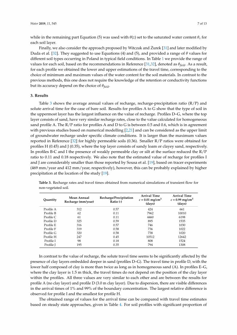
Table 3 shows the average annual values of recharge, recharge-precipitation ratio (R/P) andsolute arrival time for the case of bare soil. Results for profiles A to G show that the type of soil inthe uppermost layer has the largest influence on the value of recharge. Profiles D–G, where the toplayer consists of sand, have very similar recharge rates, close to the value calculated for homogeneoussand profile A. The R/P ratio for profiles A and D to G is between 0.5 and 0.6, which is in agreementwith previous studies based on numerical modelling [2,21] and can be considered as the upper limitof groundwater recharge under specific climate conditions. It is larger than the maximum valuesreported in Reference [32] for highly permeable soils (0.36). Smaller R/P ratios were obtained forprofiles H (0.45) and J (0.35), where the top layer consists of sandy loam or clayey sand, respectively.In profiles B-C and I the presence of weakly permeable clay or silt at the surface reduced the R/Pratio to 0.11 and 0.18 respectively. We also note that the estimated value of recharge for profiles Iand J are considerably smaller than those reported by Sousa et al. [19], based on tracer experiments(469 mm/year and 412 mm/year, respectively), however, this can be probably explained by higherprecipitation at the location of the study [19].

Table 3. Recharge rates and travel times obtained from numerical simulations of transient flow fornon-vegetated soil.

Quantity Mean AnnualRecharge (mm/year)

Recharge/PrecipitationRatio (-)

Arrival Timec = 0.01 mg/cm3

(days)

Arrival Timec = 0.99 mg/cm3

(days)

Profile A 312 0.57 424 661Profile B 62 0.11 7962 10010Profile C 61 0.11 4460 6198Profile D 325 0.59 895 1535Profile E 316 0.57 746 1030Profile F 319 0.58 736 1022Profile G 320 0.58 738 1020Profile H 247 0.45 10512 12642Profile I 98 0.18 808 1524Profile J 195 0.35 794 1308

In contrast to the value of recharge, the solute travel time seems to be significantly affected by thepresence of clay layers embedded deeper in sand (profiles D–G). The travel time in profile D, with thelower half composed of clay is more than twice as long as in homogeneous sand (A). In profiles E–G,where the clay layer is 1.5 m thick, the travel times do not depend on the position of the clay layerwithin the profiles. All three values are very similar to each other and are between the results forprofile A (no clay layer) and profile D (3.0 m clay layer). Due to dispersion, there are visible differencesin the arrival times of 1% and 99% of the boundary concentration. The largest relative difference isobserved for profile I and the smallest for profile H.

The obtained range of values for the arrival time can be compared with travel time estimatesbased on steady state approaches, given in Table 4. For soil profiles with significant proportion of

Water 2019, 11, 545 8 of 13

highly permeable materials (A, E–G) the assumption of hydrostatic distribution leads to considerablyshorter travel time than the assumption of steady downward flow. These two estimations provide arange of values that is comparable to the range of travel times calculated from transient simulations.As can be seen in Figure 1, for profile E the hydrostatic distribution of θ approximately corresponds tothe summer season and the steady flow distribution—to the winter season, with some water pondingon the top of the clay layer. A very similar range of values is obtained using the approach by Witczakand Zurek, with average values of θield reported in Table 1. Considering application of this method toprofile E, one has to note that the values of field water content θfield in Table 1 are in good agreementwith the results shown in Figure 1 for the lower part of the profile. However, in the upper sand layerthe values are generally larger, especially in winter and the clay layer remain almost fully saturated,with θ = 0.36 corresponding to the upper limit of θfield in Table 1. The lower estimates from Witczakand Zurek, which are in agreement with the early arrival of solute at the groundwater table, wereobtained for smaller values of θfield from literature, not consistent with the results of simulations.

Table 4. Estimates of travel time (days)obtained with steady-state methods for non-vegetated soil.

Method Hydrostatic Steady Flow Charbeneau & Daniel [28] Witczak & Zurek [29]

Profile A 383 655 629 491–702Profile B 12,011 12,650 11,445 8477–11,303Profile C 7106 7948 7164 5565–7539Profile D 1325 1545 1453 1044–1415Profile E 849 1124 1030 758–1044Profile F 879 1155 1057 780–1074Profile G 880 1141 1045 770–1163Profile H 12,512 12,747 12,590 12,728–13,078Profile I 1334 2121 1419 1661–2875Profile J 1111 1310 830 2003–2883

In profiles B, C and D the discrepancies between estimations based on transient and steady statemethods are larger. First, we note that hydrostatic, steady flow and Charbeneau and Daniel methodslead to similar estimates of the travel time and all three are overestimating the solute arrival time,compared to the transient simulations. Also, the results from Witczak and Zurek approach differedfrom the transient simulations more significantly than in the previous case, for the range of consideredwater contents. However, the estimate obtained for lower values of the field water content was closerto the breakthrough time obtained from SWAP.

For profile H, all methods based on steady state solutions were close to each other and predictedtravel time values close to the arrival time of 99% of input concentration in transient simulation.A good agreement between all methods for this profile can be explained by the fact, that most of itsdepth is in saturated conditions, with uniquely defined water content value.

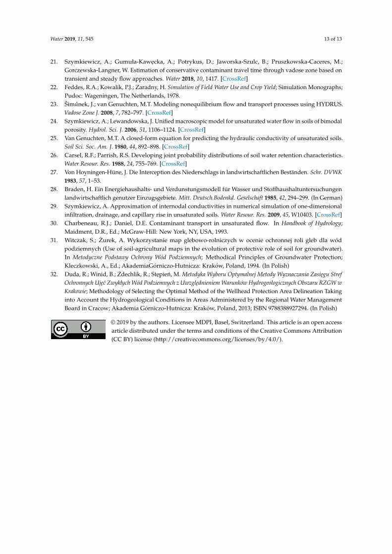
In contrast, for profiles I and J the differences between various methods were significant. In profileI the steady flow method overestimated the travel time, while both hydrostatic and Charbeneau andDaniel methods gave results comparable to the values obtained from transient simulations. In profile Jall three methods were consistent with transient simulations. In our case the differences between thehydrostatic and steady flow approach were much smaller than reported in Reference [19] for the sameprofiles but larger recharge values. For profiles I and J the method of Witczak and Zurek appearedto be less accurate than the other simplified methods, substantially overestimating the travel time.This can be explained by very low water content occurring in coarse soil materials (gravel and mediumsand), which according to transient flow, steady flow and hydrostatic results (Figure 2) is below thelower limit of field water content given in Table 1. Thus, the resulting advective velocity is larger thanpredicted by the method of Witczak and Zurek.

Water 2019, 11, 545 9 of 13Water 2019, 11, x FOR PEER REVIEW 9 of 13

(a) (b)

(c) (d)

(e) (f)

Figure 2. Volumetric water content distributions obtained from transient simulations and steady state approximations for soil profiles E and J, non-vegetated soil, (a) profile E, summer (30 Jun.), (b) profile J, summer; (c) profile E, winter (31 Dec.); (d) profile J, winter; (e) profile E, steady state, (f) profile J, steady state.

Figure 2. Volumetric water content distributions obtained from transient simulations and steady stateapproximations for soil profiles E and J, non-vegetated soil, (a) profile E, summer (30 Jun.), (b) profileJ, summer; (c) profile E, winter (31 Dec.); (d) profile J, winter; (e) profile E, steady state, (f) profile J,steady state.

Water 2019, 11, 545 10 of 13

In Table 5 we report recharge and travel time values obtained with transient simulations for soilwith grass cover. There is a significant reduction of recharge, ranging from 22% for profile H to 50%for profile I. In our previous study [21], we observed even larger decrease in homogeneous profilesof sand and silty clay. However, in that work, we assumed that the reference evapotranspirationcorresponds entirely to transpiration and the root density decreases linearly with depth. Here, a moredetailed description is used, where only a part of the reference evapotranspiration is assigned totranspiration depending on the growth of plants and the root density distribution is such that greatmajority of roots is very close to the soil surface. Consequently, there is less difference between the baresoil and grass scenarios. Keese at al. [2] also reported more significant reduction of recharge due tovegetation than obtained here, however their studies focused on locations with much higher potentialevapotranspiration. The influence of various models of root water uptake and their parameters shouldbe further investigated in conjunction with soil textural variability and climate.

Table 5. Recharge rates and travel times obtained from numerical simulations of transient flow for soilwith grass cover.

QuantityMean Annual

Recharge(mm/year)

Recharge/PrecipitationRatio (-)

Arrival Timec = 0.01 mg/cm3

(days)

Arrival Timec = 0.99 mg/cm3

(days)

Profile A 220 0.40 531 806Profile B 38 0.07 11,782 13,555Profile C 38 0.07 6336 8706Profile D 223 0.42 1480 1876Profile E 215 0.39 851 1526Profile F 224 0.41 834 1503Profile G 224 0.41 830 1501Profile H 195 0.35 12,956 15,477Profile I 52 0.09 963 1852Profile J 156 0.28 1314 1660

The travel time estimates obtained with steady state approximations for vegetated soils aresummarized in Table 6. Again, the performance of simplified methods is case-dependent. In particular,for profiles E–G the hydrostatic and steady flow methods cannot capture the early breakthroughtime of the solute and for profiles B–D they considerably overestimate the travel time even forc = 0.99 mg/cm3. In contrast, both methods still perform well in the case of homogeneous sand. Forprofiles B–D the method of Witczak and Zurek provides a range of time lag values more comparable tothe transient simulations but again, this is due to the use of smaller, literature-based water content,not corresponding to the simulation results. In profile I all steady state approximations significantlyoverpredict the solute travel time. On the other hand, in profile J the hydrostatic and steady flowmethods produce results close to the transient flow simulations, while the method of Charbeneau andDaniel leads to shorter arrival time than the one obtained from transient flow simulations. Similarlyto the non-vegetated case, the method of Witczak and Zurek predicts much longer travel times thanSWAP calculations.

Water 2019, 11, 545 11 of 13

Table 6. Estimates of travel time (days) obtained with steady-state methods for soil with grass cover.

Method Hydrostatic Steady Flow Charbeneau & Daniel [28] Witczak & Zurek [29]

Profile A 543 892 857 697–995Profile B 19,598 20,550 18,392 13,832–21,900Profile C 11,407 12,630 11,271 8933–13,832Profile D 1880 2170 2027 1482–2295Profile E 1283 1661 1514 1146–1732Profile F 1241 1598 1457 1100–1662Profile G 1257 1598 1457 1100–1662Profile H 15,849 16,120 15,926 16,116–16,565Profile I 2513 3905 2454 3131–5419Profile J 1388 1623 1011 2504–3603

4. Summary and Conclusions

Numerical simulations of transient flow and transport in layered soil profiles were compared tosimplified methods of estimating solute travel time, based on the assumption of steady flow and purelyadvective transport. Even with the relatively small value of dispersion constant used in this study(6 cm), the arrival of the solute at ground water table was spread in time. Thus, the unsaturated zonetime lag should be considered as a time interval, rather than a single value. The simplified methodsreproduced the results of transient simulations with mixed success. They performed best for profilesdominated by sand materials without vegetation. In the case of vegetated profiles or profiles withfine-textured material at the surface, the simplified method were generally not able to capture theearlier arrival time of concentration c = 0.01 mg/cm3, the results were closer to the travel time forc = 0.99 mg/cm3 but in some cases the time was greatly overestimated. It is difficult to distinguish anyof the simple methods as superior to the other ones. The methods based on hydrostatic and steady-statedistribution of the water content can be viewed as complementary in the case of coarse-textured soilsbut for fine textured soils they both predict time lags significantly longer than the transient simulations.The method based on the use of average values of the water content [29] performed quite well despiteits simplicity but the agreement with transient simulations was often obtained for values of the watercontent taken from the literature and not corresponding to the particular setting under consideration.Thus, from the point of view of practical application of this method, the use of water content valuesmeasured in the field may not necessarily lead to improved results.

This study confirmed the utility of numerical modelling as a tool to estimate groundwaterrecharge, especially due to the ease of implementing different scenarios related to lithology, vegetationand weather data. The obtained results are in agreement with earlier reports, showing the importanceof climate, soil texture in the surface layer and vegetation as the main controls of groundwaterrecharge [2–5].

Author Contributions: Conceptualization, A.S.; Methodology, A.S. and B.J.-S.; Investigation, J.S. and A.S.;Writing-Original Draft Preparation, A.S. and J.S.

Funding: The work of A.S. and B.J.-S. was funded by National Centre for Research and Development (NCBR),Poland, in the framework of the project BIOSTRATEG3/343927/3/NCBR/2017 “Modelling of the impactof the agricultural holdings and land-use structure on the quality of inland and coastal waters of the BalticSea set up on the example of the Municipality of Puck region—Integrated info-prediction Web Service WaterPUCK”—BIOSTRATEG Programme and by National Science Centre (NCN), Poland, in the framework of theproject 2015/17/B/ST10/03233 “Groundwater recharge on outwash plain. “The work of J.S. was carried outduring his stay at the Gdansk University of Technology in the framework of ERASMUS student exchangeprogramme, funded by EU.

Acknowledgments: The weather data was obtained from meteorological station of Gdansk University ofTechnology, Faculty of Civil and Environmental Engineering, Department of Hydraulic Engineering, in Sopot(54.2 N, 18.3 E). The authors would like to thank two anonymous reviewers for their suggestions.

Conflicts of Interest: The authors declare no conflict of interest.

Water 2019, 11, 545 12 of 13

References

1. Scanlon, B.R.; Christman, M.; Reedy, R.C.; Porro, I.; Simunek, J.; Flerchinger, G.N. Intercode comparisons forsimulating water balance of surficial sediments in semiarid regions. Water Resour. Res. 2002, 38. [CrossRef]

2. Keese, K.E.; Scanlon, B.R.; Reedy, R.C. Assessing controls on diffuse groundwater recharge using unsaturatedflow modeling. Water Resour. Res. 2005, 41. [CrossRef]

3. Ordens, C.M.; Post, V.E.; Werner, A.D.; Hutson, J.L. Influence of model conceptualisation on one-dimensionalrecharge quantification: Uley South, South Australia. Hydrogeol. J. 2014, 22, 795–805. [CrossRef]

4. Vero, S.E.; Ibrahim, T.G.; Creamer, R.E.; Grant, J.; Healy, M.G.; Henry, T.; Kramers, G.; Richards, K.G.;Fenton, O. Consequences of varied soil hydraulic and meteorological complexity on unsaturated zone timelag estimates. J. Contam. Hydrol. 2014, 170, 53–67. [CrossRef] [PubMed]

5. Wang, T.; Franz, T.E.; Zlotnik, V.A. Controls of soil hydraulic characteristics on modeling groundwaterrecharge under different climatic conditions. J. Hydrol. 2015, 521, 470–481. [CrossRef]

6. Fenton, O.; Vero, S.; Ibrahim, T.G.; Murphy, P.N.C.; Sherriff, S.C.; Ó hUallacháin, D. Consequences of usingdifferent soil texture determination methodologies for soil physical quality and unsaturated zone time lagestimates. J. Contam. Hydrol. 2015, 182, 16–24. [CrossRef] [PubMed]

7. Vero, S.E.; Healy, M.G.; Henry, T.; Creamer, R.E.; Ibrahim, T.G.; Richards, K.G.; Mellander, P.-E.;McDonald, N.T.; Fenton, O. A framework for determining unsaturated zone water quality time lags atcatchment scale. Agric. Ecosyst. Environ. 2017, 236, 234–242. [CrossRef]

8. Batalha, M.S.; Barbosa, M.C.; Faybishenko, B.; van Genuchten, M.T. Effect of temporal averaging ofmeteorological data on predictions of groundwater recharge. J. Hydrol. Hydromech. 2018, 66, 143–152.[CrossRef]

9. Szymkiewicz, A.; Gumuła-Kawecka, A.; Šimunek, J.; Leterme, B.; Beegum, S.; Jaworska-Szulc, B.;Pruszkowska-Cacers, M.; Gorczewska-Langner, W.; Jacques, D. Simulations of freshwater lens recharge andsalt/freshwater interfaces using the HYDRUS and SWI2 packages for MODFLOW. J. Hydrol. Hydromech.2018, 66, 246–256. [CrossRef]

10. Bashir, R.; Pastora Chevez, E. Spatial and seasonal variations of water and salt movement in the vadose zoneat salt-impacted sites. Water 2018, 10, 1833. [CrossRef]

11. Zhou, Y.; Wang, X.S.; Han, P.F. Depth-dependent seasonal variation of soil water in a thick vadose zone inthe Badain Jaran Desert, China. Water 2018, 10, 1719. [CrossRef]

12. Beegum, S.; Šimunek, J.; Szymkiewicz, A.; Sudheer, K.P.; Nambi, I.M. Implementation of solute transport inthe vadose zone into the ‘HYDRUS package for MODFLOW’. Groundwater 2018. [CrossRef]

13. Šimunek, J.; Šejna, M.; Saito, H.; Sakai, M.; van Genuchten, M.T. The HYDRUS-1D Software Package forSimulating the One-Dimensional Movement of Water, Heat, and Multiple Solutes in Variably-Saturated Media,Version 4.0; HYDRUS Software Series 3; University of California: Riverside, CA, USA, 2008.

14. Kroes, J.G.; van Dam, J.C.; Bartholomeus, R.P.; Groenendijk, P.; Heinen, M.; Hendriks, R.F.A.; Mulder, H.M.;Supit, I.; van Walsum, P.E.V. SWAP Version 4. Theory Description and User Manual; Report 2780; WageningenUniversity & Research: Wageningen, The Netherlands, 2017.

15. Fayer, M.J.; Jones, T.L. UNSAT-H Version 2.0: Unsaturated Soil Water and Heat Flow Model (No. PNL-6779);Pacific Northwest Lab.: Richland, WA, USA, 1990.

16. Schroeder, P.R.; Dozier, T.S.; Zappi, P.A.; McEnroe, B.M.; Sjostrom, J.W.; Peton, R.L. The Hydrologic Evaluationof Landfill Performance (HELP) Model: Engineering Documentation for Version 3; EPA/600/R-94/168b; US.Environmental Protection Agency, Risk Reduction Engineering Laboratory: Cincinnati, OH, USA, 1994.

17. Charbeneau, R.J. Groundwater Hydraulics and Pollutant Transport; Waveland Press: Long Grove, IL, USA, 2006;ISBN 1478608315.

18. Fenton, O.; Schulte, R.P.; Jordan, P.; Lalor, S.T.; Richards, K.G. Time lag: A methodology for the estimation ofvertical and horizontal travel and flushing timescales to nitrate threshold concentrations in Irish aquifers.Environ. Sci. Policy 2011, 14, 419–431. [CrossRef]

19. Sousa, M.R.; Jones, J.P.; Frind, E.O.; Rudolph, D.L. A simple method to assess unsaturated zone time lag inthe travel time from ground surface to receptor. J. Contam. Hydrol. 2013, 144, 138–151. [CrossRef]

20. Potrykus, D.; Gumuła-Kawecka, A.; Jaworska-Szulc, B.; Pruszkowska-Caceres, M.; Szymkiewicz, A.Assessing groundwater vulnerability to pollution in the Puck region (denudation moraine upland) usingvertical seepage method. E3S Web Conf. 2018, 44, 00147. [CrossRef]

Water 2019, 11, 545 13 of 13

21. Szymkiewicz, A.; Gumuła-Kawecka, A.; Potrykus, D.; Jaworska-Szulc, B.; Pruszkowska-Caceres, M.;Gorczewska-Langner, W. Estimation of conservative contaminant travel time through vadose zone based ontransient and steady flow approaches. Water 2018, 10, 1417. [CrossRef]

22. Feddes, R.A.; Kowalik, P.J.; Zaradny, H. Simulation of Field Water Use and Crop Yield; Simulation Monographs;Pudoc: Wageningen, The Netherlands, 1978.

23. Šimunek, J.; van Genuchten, M.T. Modeling nonequilibrium flow and transport processes using HYDRUS.Vadose Zone J. 2008, 7, 782–797. [CrossRef]

24. Szymkiewicz, A.; Lewandowska, J. Unified macroscopic model for unsaturated water flow in soils of bimodalporosity. Hydrol. Sci. J. 2006, 51, 1106–1124. [CrossRef]

25. Van Genuchten, M.T. A closed-form equation for predicting the hydraulic conductivity of unsaturated soils.Soil Sci. Soc. Am. J. 1980, 44, 892–898. [CrossRef]

26. Carsel, R.F.; Parrish, R.S. Developing joint probability distributions of soil water retention characteristics.Water Resour. Res. 1988, 24, 755–769. [CrossRef]

27. Von Hoyningen-Hüne, J. Die Interception des Niederschlags in landwirtschaftlichen Beständen. Schr. DVWK1983, 57, 1–53.

28. Braden, H. Ein Energiehaushalts- und Verdunstungsmodell für Wasser und Stoffhaushaltuntersuchungenlandwirtschaftlich genutzer Einzugsgebiete. Mitt. Deutsch.Bodenkd. Geselschaft 1985, 42, 294–299. (In German)

29. Szymkiewicz, A. Approximation of internodal conductivities in numerical simulation of one-dimensionalinfiltration, drainage, and capillary rise in unsaturated soils. Water Resour. Res. 2009, 45, W10403. [CrossRef]

30. Charbeneau, R.J.; Daniel, D.E. Contaminant transport in unsaturated flow. In Handbook of Hydrology;Maidment, D.R., Ed.; McGraw-Hill: New York, NY, USA, 1993.

31. Witczak, S.; Zurek, A. Wykorzystanie map glebowo-rolniczych w ocenie ochronnej roli gleb dla wódpodziemnych (Use of soil-agricultural maps in the evolution of protective role of soil for groundwater).In Metodyczne Podstawy Ochrony Wód Podziemnych; Methodical Principles of Groundwater Protection;Kleczkowski, A., Ed.; AkademiaGórniczo-Hutnicza: Kraków, Poland, 1994. (In Polish)

32. Duda, R.; Winid, B.; Zdechlik, R.; Stepien, M. Metodyka Wyboru Optymalnej Metody Wyznaczania Zasiegu StrefOchronnych Ujec Zwykłych Wód Podziemnych z Uwzglednieniem Warunków Hydrogeologicznych Obszaru RZGW wKrakowie; Methodology of Selecting the Optimal Method of the Wellhead Protection Area Delineation Takinginto Account the Hydrogeological Conditions in Areas Administered by the Regional Water ManagementBoard in Cracow; Akademia Górniczo-Hutnicza: Kraków, Poland, 2013; ISBN 9788388927294. (In Polish)

© 2019 by the authors. Licensee MDPI, Basel, Switzerland. This article is an open accessarticle distributed under the terms and conditions of the Creative Commons Attribution(CC BY) license (http://creativecommons.org/licenses/by/4.0/).