0097-8078/05/3203- © 2005

MAIK “Nauka

/Interperiodica”0291

Water Resources, Vol. 32, No. 3, 2005, pp. 291–304. Translated from Vodnye Resursy, Vol. 32, No. 3, 2005, pp. 322–336.Original Russian Text Copyright © 2005 by Dolgonosov, Gubernatorova.

INTRODUCTION

The self-purification capacity of aquatic environ-ment can be characterized by the rate of solute transfor-mations. In the problems of solute migration, its decayis commonly described by a first-order reaction equa-tion [1]. This model is often found to be inadequate. Amore accurate description can be derived from the realtransformation mechanisms (biological, chemical, andphysicochemical [6, 7]), which are described by vari-ous nonlinear models [5] describing heterogeneous,self-catalyzed, enzymatic, and biochemical reactions.However, the complexity of such models restricts theirapplication; therefore, an urgent task is the develop-ment of a generalized nonlinear model that will reflectthe common features of different mechanisms of solutetransformations but will not involve too complicatedtheoretical schemes.

When solving this problem, one should take intoaccount that the solute is commonly a class of substancesof similar nature, rather than an individual substance. Itsspecific feature is the variability of kinetic characteristicsof its components as a function of their chemical struc-ture and molecular mass. Examples of these are humicsubstances, phenols, lignins, petroleum hydrocarbons,dioxins, detergents, and the like. Each such class con-tains a range of compounds with different reactivity (bio-availability, lability, and so on) with respect to differentbiological, chemical, and physicochemical effects. Thedecay of a multicomponent mixture begins with thedecomposition of the most labile compounds, afterwhich more stable compounds become involved in theprocess [14]. The latter compounds will play the leadingrole at later stages of the decay process.

The overall rate of the process which reflects thedecay of all components depends on their proportionsin the mixture. When the share of stable components islarge, their decay will be extended over a longer periodthan it can be expected if a first-order reaction is

assumed to take place. The concentrations of solutes inthe aquatic environment will remain high, thus reduc-ing the admissible pollution level of the water body, andwhen pollutants are discharged repeatedly, their con-centrations can reach catastrophic levels, which willhave adverse effect on water quality and the vital activ-ity of the aquatic biota [3].

This reasoning applies not only to the water columnbut also to bottom sediments, which accumulate manypollutants entering a water body. The main mechanismof self-purification of bottom sediments is biodegrada-tion of organic matter, which can proceed both in aero-bic and anaerobic conditions under the effect of differ-ent microorganism groups. Analysis of published dataon the distribution of organic matter in a bottom-sedi-ment core shows that, depending on the assimilabilityof the substance, the time of its decay can vary from afew hours to several years, and in deep-sea marine sed-iments, it can reach even several million years [22].

The objective of this study is the development of ageneralized model of solute transformations and analy-sis of this model based on published data on the kineticsof self-purification processes in the aquatic environ-ment, such as biodegradation, bioaccumulation, photo-destruction of solutes, and sedimentation of particulatematter along with adsorbed solutes.

DECOMPOSITION OF A MULITCOMPONENT SOLUTE

As it was mentioned in [14], organic matter consistsof various groups of compounds, which feature differ-ent reactivity with respect to decay. It was assumed thatthe decay of each group can be described by a first-order reaction equation. On this basis, a polyfractionmodel was suggested. In this model, the rate of organicmatter decay is represented as a sum of first-order termsdescribing the decay of its individual groups.

A Nonlinear Model of Contaminant Transformations in an Aquatic Environment

B. M. Dolgonosov and T. N. Gubernatorova

Water Problems Institute, Russian Academy of Sciences, ul. Gubkina 3, GSP–1, Moscow, 119991 Russia

Received August 30, 2004

Abstract

—A nonlinear model of the decomposition of a multicomponent contaminant is developed with allow-ance made for the distribution of components over their reactivity. Model application is illustrated by the anal-ysis of published empirical data on organic matter biodegradation in water column and bottom sediments, in anactivated-sludge bioreactor, and the biological absorption and enzymatic destruction of organic matter by mac-rophytes. Photodestruction, chemical destruction, and sedimentation are also considered. The nonlinear modelis compared with a first-order reaction equation.

WATER QUALITY AND PROTECTION:ENVIRONMENTAL ASPECTS

292

WATER RESOURCES

Vol. 32

No. 3

2005

DOLGONOSOV, GUBERNATOROVA

As the number of fractions increases, the number ofempirical parameters of the model also increases, thusreducing its prognostic capacity since the calibration ofsuch model requires too vast body of experimental data.

The polyfraction model involves aggregative frac-tions, each embracing a wide range of compounds. Letus consider what we can benefit from the transitionfrom fractions to individual components (compounds),that is, from the replacement of a discrete division intofractions by a continuous distribution over the reactivi-ties of individual components.

As before, we assume that the decay of an individualcomponent follows the first-order reaction equation:

which yields the exponential function for the concen-tration:

where

k

is the reactivity of the component (reactionconstant);

c

k

and

c

k

0

are the current and initial concen-trations of the component;

t

is the time. Each compo-nent has its own

k

value. The total concentration oforganic matter equals the sum of the concentrations ofall individual components. In the case of continuousdistribution over

k

, the sum must be replaced by theintegral,

where

c

k

should be regarded as a distribution densityover

k

; considering the exponential decay of each indi-vidual component, this yields

(1)

dck/dt kck,–=

ck ck0 kt–( ),exp=

c ck k,d

0

∞

∫=

c ck0e kt– k.d

0

∞

∫=

This relationship can be interpreted as a superpositionof the contributions of individual components.

According to (1), the dependence of organic matterconcentration on time is completely determined by thevalue of

c

k

0

(the initial distribution of components overthe reactivity). The form of this distribution is to befound.

Analysis of the available empirical data [26] sug-gests that the multicomponent organic matter includesboth a labile (readily decomposable) and a stable (diffi-cultly decomposable) fraction. The former has largervalues of the reactivity

k

, while the latter has smallervalues.

The decomposition of the labile fraction can becharacterized by a time

T

, within which its concentra-tion notably drops. In this case, the distribution densityof the reactivity for large

k

can be described by theexponent exp

(–

kT

)

.By contrast, stable components do not have a char-

acteristics decay time. In this case, the distribution den-sity for small

k

values should be described by a powerlaw

k

α

(in this case, there is an analogy with the flicker-noise [13, 20, 21], for which no characteristic timeexists).

Combining these two cases, we can write the overalldistribution density in the form

(2)

The constant

A

can be found from the normalizationcondition:

where

c

0

is the initial concentration of organic matter.For the integral to exist, the condition

α

> –1 must besatisfied. Integration under this condition yields

where

Γ

is gamma function. Depending on the values ofparameter

α

, we have two types of distribution (Fig. 1):at –1 <

α

≤

0

, we have a monotonically decreasingdistribution with an integrable singularity at

α

= 0;at

α

> 0, the distribution is nonmonotonic and has amaximum at

k

=

α

/

T

.The overall concentration of organic matter can be

found through the substitution of (2) in (1). After sim-ple transformations, we obtain:

(3)

Thus, even if the decay of individual components isdescribed by an exponent, the decay of organic matteras a whole follows the law (3), which has an asymptot-ically power character.

ck0 Akα kT–( ).exp=

c0 ck0 k,d

0

∞

∫=

A c0Tα 1+ /Γ α 1+( ).=

cc0

1 t/T+( )α 1+------------------------------.=

c

k

0

/(

c

0

T

)0.6

0.2

0 1 2

kT

1

2

Fig. 1.

Reactivity distribution for components: (1) at

–1 <

α

≤

0

; (2) at

α

> 0 (the calculations were made at

α

= –0.5and 1).

WATER RESOURCES

Vol. 32

No. 3

2005

A NONLINEAR MODEL OF CONTAMINANT TRANSFORMATIONS 293

The existence of a power asymptote instead of expo-nential decay (following from the first-order equation)for the processes of self-purification was first men-tioned in [3].

It can be easily shown that (3) suggests a kineticequation of the type (5). This result will be obtainedbelow in another way.

NONLINEAR MODEL

The biodegradation of organic matter is controlledby enzymatic reactions, the kinetics of which isdescribed by the Moser equation [23]

(4)

where

c

is the concentration of organic matter;

X

is thebiomass of the enzyme-producing organisms;

µ

is thespecific rate of decomposition;

K

is the half-saturationconstant;

ν

is the order of the enzymatic reaction (

ν

> 0).Let us take into account that the self-purification

capacity of the natural aquatic environment persists onlyif the solute concentration is sufficiently low

c

�

K

. Thisallows (4) to be reduced to the equation

(5)

(

k

=

µ

X

/Kν is the reaction constant), which, in terms ofchemical kinetics, describes a νth-order reaction. Aswill be shown below, the nonlinear model (5) can bealso applied to the cases other than enzymatic decom-position (chemical oxidation, photodestruction of amulticomponent solute, sedimentation of a coagulatingsuspension), though in the form of an interpolationequation.

Let us consider the mathematical aspects of model(5), which will be used in the analysis of empiricalmaterial.

At constant k, (5) has the solution of the form

(6)

(7)

where c0 is the initial concentration of the solute.Depending on the value of ν, we have the following

three particular cases.At ν < 1,

(8)

As can be seen from (8), at ν < 1, the solute decom-poses completely within a finite time T.

The particular case ν = 1, corresponds to the con-ventional linear dynamics dc/dt = –kc and yields theexponential decomposition law (7).

In the case of ν > 1, expression (6) can be conve-niently represented in the form

dcdt------ µX

cν

cν Kν+-----------------,–=

dc/dt kcν–=

c c0 1 ν 1–( )c0ν 1– kt+[ ]1/ 1 ν–( )

, ν 1;≠=

c c0e kt– , ν 1,= =

c c0 1 t/T–( )1/ 1 ν–( ), T c01 ν– / k 1 ν–( )[ ].= =

(9)

where

(10)

The result (9) coincides with (3) at ε = α + 1. There-fore, nonlinear equation (5) corresponds to the spec-trum of reactivities of the components:

An important consequence of (9) is the fact that atlarge time t � T, there exists a power asymptoticapproximation

(11)

T in (9) characterizes the duration of the initial phase ofthe decomposition of labile fraction. The characteristictime t0 of the entire process can be found from the rela-tionship

(12)

Substituting (12) in (9), we find that the integralin (12) exists only at ε > 1, that is, at 1 < ν < 2. The inte-gration yields

(13)

from which it follows that t0 is proportional to T.When ε ≤ 1 (or ν > 2), the integral in (12) does not

exist, and hence the characteristic time cannot be intro-duced for the process, which lasts infinitely. The dura-tion of the real process will be far in excess of the dura-tion of the initial phase T.

Let us analyze the kinetics of individual self-purifi-cation processes including biodegradation, bioaccumu-lation, chemical and photodestrustion, and sedimenta-tion with the aim to determine whether the nonlinearmodel described above can be applied to the descrip-tion of each process.

BIODEGRADATION OF ORGANIC MATTERIN BOTTOM SEDIMENTS

A vast body of experimental and field data on therate of organic matter decomposition in marine bottomsediments were considered in [22]. The description wasbased on the conventional kinetics of first-order reac-tion, but the kinetic coefficient was assumed to be time-dependent (the so-called quasi-first-order reaction [2])

(14)

This equation has the solution of the form

cc0

1 t/T+( )ε-----------------------,=

Tε

kc01/ε-----------, ε 1

ν 1–------------.= =

ck t( ) ck0 kt–( )exp=

= c0Tε/Γ ε( )[ ]kε 1– k t T+( )–[ ].exp

c t ε– .∼

c0t0 c t( ) t,d

0

∞

∫=

t0 T / ε 1–( ), ε 1,>=

dc/dt κ t( )c.–=

294

WATER RESOURCES Vol. 32 No. 3 2005

DOLGONOSOV, GUBERNATOROVA

(15)

In [22], the time dependence of the kinetic coeffi-cient had a power form

(16)

and adequately described the decomposition kinetics atthe later phase of the process. The value of the exponentwas found to be close to unity. Processing of the entirebody of empirical data yielded the value of a = 0.95 ±0.01, and the same procedure applied only to the exper-imental data (regarded as most accurate) isolated fromthe whole data body yielded a = 1.00 ± 0.06. Moreover,the value of the coefficient of proportionality in (16)was obtained, and this relationship took the form:

(17)

The relationship (17) can be derived theoreticallyfrom the following considerations. The dependence ofκ on t in (14) follows from the relationship between κand solute concentration. If we take equation (5) as abasis, the correlation of (14) and (5) results in the rela-tionship κ = kcν – 1. Substituting (9) in this equation withallowance made for the definitions of values (10) yields

(18)

At t � T, we obtain

(19)

From the comparison of (17) and (19), it follows thatε = 0.14.

To describe not only the asymptotic phase (11), butalso the initial segment of the decomposition curve, thefollowing formula was used in [22]:

(20)

This formula was first proposed in [17]. At t � T, thedependence (20) changes to (16). At a = 1, we obtainthe time dependence of the type of (18).

An important result obtained in [22] is the fact thatthe exponent a in (16) and (20) is close to unity. Thisallows us to take this coefficient equal to unity. Now,the substitution of (20) (at a = 1) into (15) and integra-tion give the result completely identical with (9).

Thus, we have serious reasons to believe that thebiodegradation of organic matter in bottom depositscan be described by the same nonlinear model (5) withan effective order of reaction ν = 1 + ε–1 = 8.1.

DECOMPOSITION OF PLANKTONIC DETRITUS IN BOTTOM SEDIMENTS

A particular case of the polyfraction model [14]with three groups of compounds (labile, difficultlydecomposable, and undecomposable) was considered

c c0 κ t'( ) t'd

0

t

∫–

.exp=

κ t a–∼

κ 0.14t 1– .=

κ ε/ T t+( ).=

κ εt 1– .=

κ T t+( ) a– ,∼

in [26]. Experiments were made with samples of anaer-obic marine sediments, to which specially treatedplanktonic detritus was later added. It was composed offractions of different age, which had decomposed underanaerobic conditions for a long time. This ensures thepresence of organic matter with different assimilabilityin the detritus.

The decomposition of organic matter in the preparedartificial sediments was made by a microbial commu-nity of natural origin under anaerobic conditions. Thiscommunity tends to successively decompose organicsubstrates starting from the most readily assimilableand passing to the more stable. First, enzymatic micro-organisms hydrolyze the original detritus to producelow-molecular compounds, which are then utilized bysulfate-reducing bacteria. The original sediments wererich in dissolved sulfate, which stimulated the processof bacterial sulfate reduction after the addition of detri-tus. The concentrations of total and particulate organiccarbon were measured in the experiment.

In accordance with the accepted three-fractionmodel, the equation of organic matter decompositionwas obtained in the form

(21)

where c is the current concentration of organic matter,c01, c02, and c03 are the initial concentrations of the frac-tions of labile, difficultly decomposable, and undecom-posable organic matter, respectively; k1 and k2 are thereactivities of the first two fractions, respectively (k3 = 0).The sum c01 + c02 + c03 = c0 yields the initial concentra-tion of organic matter, c0. A plausible, though not veri-fied, assumption used in the model is that both thedecomposable fractions will be completely mineral-ized, while the undecomposable fraction does notchange. (It is not supplemented by the products ofdecomposition of the first two fractions, although thiscannot be ruled out.)

Processing of experimental data on particulateorganic matter yielded the following values for theparameters of model (21):

(22)

The labile fraction has a greater value of k, and hencesmaller decomposition time k–1.

The decrease in organic matter concentration com-prised two stages: the rapid initial decay and the subse-quent slow decomposition.

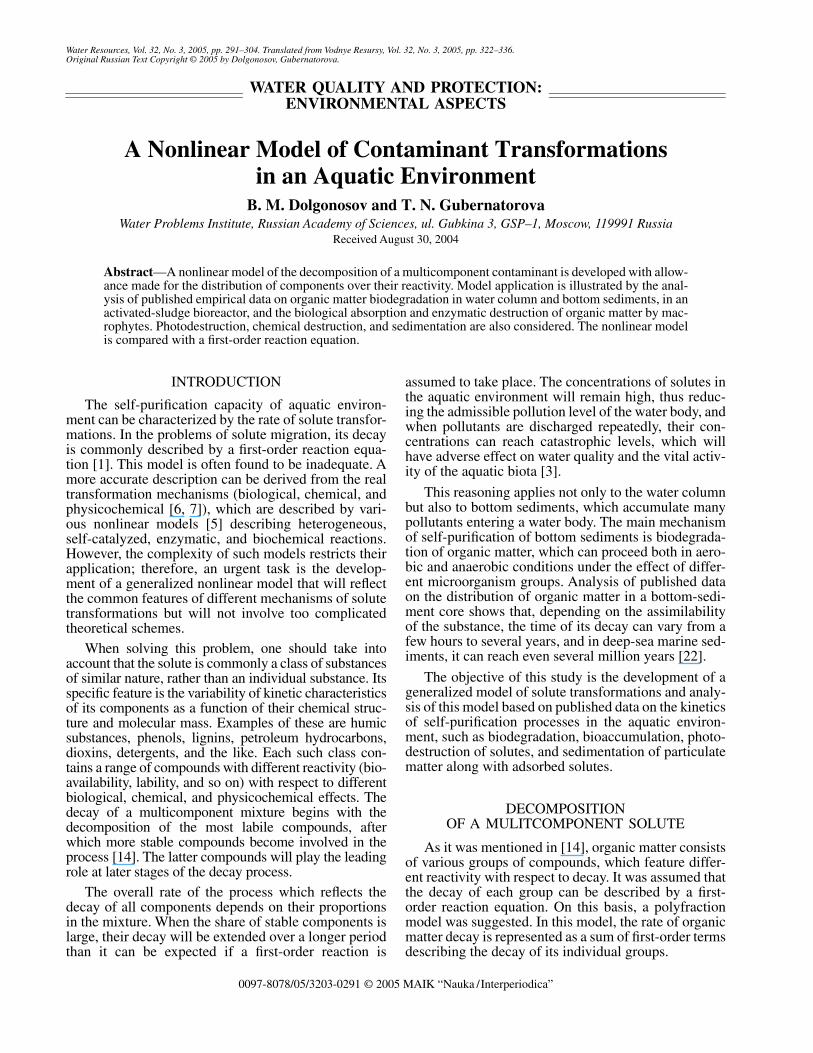
Let us use model (5) to process the experimentaldata from [26] (Fig. 2). The full curve was constructedby using the least-squares method from equation (9).The parameter values thus obtained are: ε = 0.14, T =0.30 day. The standard deviation of experimental valuesfrom the theoretical curve amounts to σ = 1.7%. The

c c01 k1t–( )exp c02 k2t–( )exp c03,+ +=

c0 1.81 gC/l, c01/c0 0.50, c02/c0 0.16,= = =

c03/c0 0.34,=

k1 24 year 1– , k2 1.4 year 1– .= =

WATER RESOURCES Vol. 32 No. 3 2005

A NONLINEAR MODEL OF CONTAMINANT TRANSFORMATIONS 295

short duration of the first stage suggests the presence oflabile organic matter utilized by microorganisms withina few hours. The effective order of reaction (5) at thegiven value of ε is equal to ν = 8.1.

The dashed line also shown in Fig. 2 is described bythe three-fraction model (21) with parameters (22).

The comparison of theoretical curves shows thatboth approximations adequately describe the measureddata. The initial part of the plot, where the deviation ismaximum, contains only two experimental points,which is obviously too few to discriminate between themodels. In this case, the most important factor will bethe simplicity of the model, which is determined by thenumber of empirical parameters. Based on this crite-rion, the nonlinear model (5), which contains only twoparameters ε and T (if we assume that the initial concen-tration of organic matter is specified) should be preferredto the linear three-fraction model (21), which containsfour independent parameters c01, c02, k1, and k2.

DESTRUCTION OF ORGANIC MATTERIN AN ACTIVE-SLUDGE BIOREACTOR

The destruction of organic matter in a bioreactor isregarded as an analogue of the processes taking place inthe natural aquatic environment (although at a lowerrate) when municipal wastewater is discharged into it.

Transformation of organic matter under the effect ofactive-sludge microorganisms in a bioreactor was ana-lyzed in [2]. It was shown that, at integrated treatment,when substrate concentrations in the reactor are low,the kinetics of organic matter biodegradation can beadequately described by Fair model [15], which can bereadily reduced to the form (5).

When used to treat experimental data on the oxida-tion kinetics of various substrates, this model yields ν =1.7–2 for peptone–starch mixture and ν = 3 for munic-ipal wastewaters (Figs. 24 and 25 in [2]). This allows usto find the characteristic values of ε in (9) and (10): ε =1–1.4 for peptone–starch mixture, and ε = 0.5 formunicipal wastewater.

Destruction of organic matter from domestic waste-water in a bioreactor is considered in [19]. Two stagesof this process are described. The first stage—anintense aerobic biodegradation—is characterized by arapid decomposition of particulate organic matter, anincrease in dissolved organic matter and the beginningof its decomposition, and an exponential growth in thebiomass of microorganisms. At the second stage, lim-ited aerobic biodegradation takes place. During it, theparticulate organic matter almost does not change, thedissolved organic matter continues dissolving, and thebiomass remains at a constant level. The decompositionkinetics of dissolved organic matter at the second stageis described by Moser equation (4), which can bereduced to the model (5) at low concentrations of sub-strate.

A model, formalizing the described two-stagedecomposition kinetics, was developed in [19] and usedto process experimental data. It was shown that, withvariations in the initial concentration of organic matter,parameter ν irregularly varies within an interval of 0.6–9.6, which is seen to overlap with the domain ν < 1.This result differs from the data in [2], where ν > 1 inall cases. The appearance of values ν < 1 can be an arte-fact caused by the complexity of the model used, inac-curacy of the experimental data, and clearly the incor-rectness (in the mathematical sense) of the inverseproblem of search for the model parameters based onthe minimization of the discrepancy functional. Never-theless, it will be recalled that at ν < 1, the decomposi-tion of organic matter will be completed within a finitetime, while at ν > 1, the later stages of its decomposi-tion can be asymptotically described by a power func-tion c ~ t –ε (ε, see (10)). In the latter case, at 1 < ν < 2(or at ε > 1), the process will be basically completedwithin a time period of the order of t0 (see (13)), whileat ν ≥ 2 (ε ≤ 1), the process is slower and its durationwill be much longer than the length T of its initial stage.

DECOMPOSITION OF LIGNINS

Results obtained in experimental studies of destruc-tion of lignin substances isolated from wastewatersfrom pulp and paper mills in eastern Siberia are givenin [9]. The measurements were made in water fromLake Baikal and the Angara River, into which a solutionof lignin with a specified concentration was introduced.A combined water–bottom sediment system was alsostudied. Vessels without addition of lignin were used asa check test. The experiment lasted for 20 months. Theconcentration of lignin (by optical method), chemicaloxygen demand (COD), color index, and other charac-teristics were measured approximately once a month.

c, g/l

1.7

1.3

0.9

0.50 200 600

t, day

Fig. 2. Kinetics of aerobic decomposition of planktonicdetritus in bottom sediments (experimental data [26]): c isthe concentration of particulate organic matter.

296

WATER RESOURCES Vol. 32 No. 3 2005

DOLGONOSOV, GUBERNATOROVA

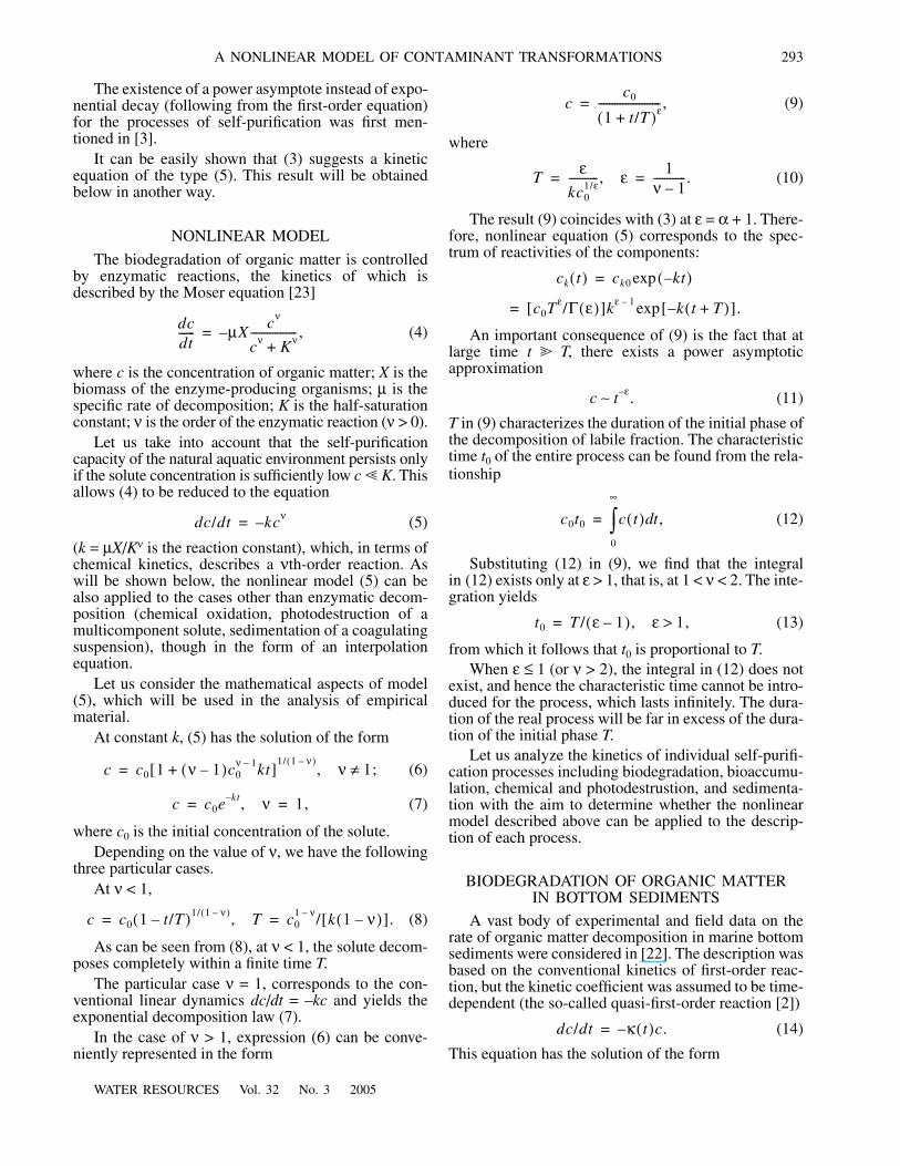
Experimental data [9] for these three characteristicswere treated using formula (9). The parameters wereevaluated using the least-squares method (Table 1).

For the comparison of calculation results withexperimental data, Fig. 3 gives the kinetic curves,obtained by using equation (9), along with the curve ofexponential decay corresponding to a first-order reac-tion and constructed with the use of the least-squaresmethod. The nonlinear model is seen to better fit theresults of measurements than the conventional linearmodel.

Analysis of Table 1 and Fig. 3 suggests the follow-ing conclusions:

Regarding the lignin content: in three cases out offour, ε and T ∞, though their ratio is finite. In thesecases, lignin concentration varies in accordance withthe exponential law exp(–kt), where k = ε/T (that is, it isdescribed by a first-order reaction equation). In onecase, the decay deviates from the exponential law andis characterized by ε < 1. These deviations can be attrib-uted to the variations in the chemical composition oflignins and the structure of microorganism communi-ties that process lignins. These factors were not con-trolled in the experiment.

Regarding COD and color index: variations in waterquality characteristics in all cases are adequately

0.8

0.4

1.0

0.6

0.2

0.8

0.4

0.8

0.4

0.8

0.4

0

0.8

0.4

0

0.8

0.4

0

0.8

0.4

00 400

0 400

0 400

0 400 400

400

400

400

Color index Color index

COD

COD

(a) (b)

(c) (d)

(e) (f)

(g) (h)

t, dayt, day

Fig. 3. Kinetics of lignin decomposition (based on data from [9]). Experimental system: water without bottom sediments (a, c, e, g),water with bottom sediments (b, d, f, h); (a, b, e, f) water from the Angara River; (e, d, g, h) water from Lake Baikal. The full curvewas calculated by (9), the dashed curve is an exponential approximation (first-order kinetics); parameters of the curves are givenin Table 1.

WATER RESOURCES Vol. 32 No. 3 2005

A NONLINEAR MODEL OF CONTAMINANT TRANSFORMATIONS 297

described by equation (9) with finite values of ε and T.The values of parameters averaged for these character-istics are given in Table 2. The exponent ε in the water–bottom sediment system is greater than that withoutbottom sediment. This can be due to the faster decreasein these characteristics with time in the presence of bot-tom sediments because of sorption and transformationof the solute in the sediments. In the cases where ε < 1,the decay will last for a considerable time, which ismuch greater than the duration of the initial stage of theprocess (which equals to about 100 days). For theBaikal water–bottom sediment system, ε > 1. Accord-ing to (13), the decay in most cases has the characteris-tic time of ~280 day.

The order of reaction ν in accordance with Table 1lies within 1–3.7. In all cases, equation (9) can be usedto describe the kinetics of lignin decomposition as canbe seen from the small scatter of experimental pointsaround the theoretical curve (the standard deviation is2–5%).

As can be seen from Table 1, the order of reaction νevaluated from measurements in lignin concentrationfails to agree with that for the color index and COD. Thisappears to be due to the indirect determination of lignin(optical methods were used). The point is that the mea-sured optical density is an integral characteristic, and dif-

ferent combinations of components in a mixture oflignins can yield the same value of this density. Differentlignins may have different decomposition times, whichcan be the reason of the aforementioned deviation.

DECOMPOSITION OF CHLOROLIGNINS

Kinetic data presented in [10] describe the decom-position of chlorolignins that form at different stages ofpulp and paper production, in particular, during chlori-nation of sulphate lignin in an acid environment, analkaline environment, and during their release frombleaching lye. These substances pass through biologi-cal treatment facilities without changes and reach waterbodies. The majority of lignins are high-molecular-mass compounds (1000–10 000), which decompose innatural aquatic environment to yield chlorophenols andother low-molecular-mass compounds with higher tox-icity and mutagenicity.

The decomposition of lignins was studied in [10]with the use of the experimental method that wasapplied in [9] to studying lignins. The duration of theexperiment was 1.5 year.

The measured data were processed based on the the-oretical relationship (9). Plots of water quality charac-teristics (chlorolignin content, COD, color index) ver-

1.0

0.8

0.6

1.0

0.8

0.6

0.4

1.0

0.8

0.6

0.4

0.8

0.4

1.0

0.8

0.6

0.4

1.0

0.8

0.6

0 200 400 0 200 400

Lignin concentration Color index

Lignin concentrationCOD

Color index COD

t, day

(a) (b)

(c) (d)

(e) (f)

Fig. 4. Kinetics of decomposition of chlorolignins obtained by chlorination of sulfate lignin in an alkaline medium (according todata from [10]). Experimental system: (a–c) water without bottom sediments; (d–f) water with bottom sediments. The values on theordinate axis are water quality characteristics (the proportion of the initial value). The full curve was calculated by (9), the dashedcurve is an exponential approximation; parameters of the curves are given in Table 3.

298

WATER RESOURCES Vol. 32 No. 3 2005

DOLGONOSOV, GUBERNATOROVA

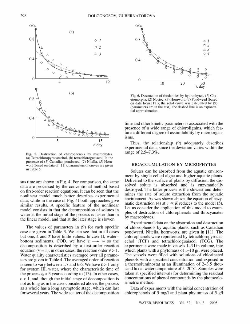
sus time are shown in Fig. 4. For comparison, the samedata are processed by the conventional method basedon first-order reaction equations. It can be seen that thenonlinear model much better describes experimentaldata, while in the case of Fig. 4f both approaches givesimilar results. A specific feature of the nonlinearmodel consists in that the decomposition of solutes inwater at the initial stage of the process is faster than inthe linear model, and that at the later stage is slower.

The values of parameters in (9) for each specificcase are given in Table 3. We can see that in all casesbut one, ε and T have finite values. In case II, water–bottom sediments, COD, we have ε ∞ so thedecomposition is described by a first-order reactionequation (ν = 1); in other cases, the reaction order ν > 1.Water quality characteristics averaged over all parame-ters are given in Table 4. The averaged order of reactionis seen to vary between 1.7 and 6.6. We have ε > 1 onlyfor system III, water, where the characteristic time ofthe process t0 > 3 year according to (13). In other cases,ε < 1, and, though the initial stage of decomposition isnot as long as in the case considered above, the processas a whole has a long asymptotic stage, which can lastfor several years. The wide scatter of the decomposition

time and other kinetic parameters is associated with thepresence of a wide range of chlorolignins, which fea-ture a different degree of assimilability by microorgan-isms.

Thus, the relationship (9) adequately describesexperimental data, since the deviation varies within therange of 2.5–7.3%.

BIOACCUMULATION BY MICROPHYTES

Solutes can be absorbed from the aquatic environ-ment by single-celled algae and higher aquatic plants.Delivered to the surface of plants by diffusion, the dis-solved solute is absorbed and is enzymaticallydestroyed. The latter process is the slowest and deter-mines the rate of solute extraction from the aquaticenvironment. As was shown above, the equation of enzy-matic destruction (4) at c � K reduces to the model (5).Let us consider the application of this model to exam-ples of destruction of chlorophenols and thiocyanatesby macrophytes.

Experimental data on the absorption and destructionof chlorophenols by aquatic plants, such as Canadianpondweed, Nitella, hornworts, are given in [11]. Thechlorophenols were represented by tetrachloropyrocat-echol (TCP) and tetrachloroguaiacol (TCG). Theexperiments were made in vessels 1–3 l in volume, intowhich plants with a phytomass of 1–10 g/l were placed.The vessels were filled with solutions of chlorinatedphenols with a specified concentration and exposed ina thermoluminostat at an illumination of 2–3.5 thou-sand lux at water temperature of 5–20°ë. Samples weretaken at specified intervals for determining the residualconcentrations of phenol compounds by the photocolo-rimetric method.

Data of experiments with the initial concentration ofchlorophenols of 5 mg/l and plant phytomass of 5 g/l

c/c0

0.8

0.4

04 12

1

2

3

0.8

0.4

05 15

t, day

(a)

(b)

Fig. 5. Destruction of chlorophenols by macrophytes.(a) Tetrachloropyrocatechol, (b) tetrachloroguaiacol. In thepresence of (1) Canadian pondweed, (2) Nitella, (3) Horn-wort (based on data of [11]); parameters of curves are givenin Table 5.

c/c0

0.8

0.4

010 20 30

t, day

1234

Fig. 6. Destruction of rhodanides by hydrophytes. (1) Cha-etomorpha, (2) Nostoc, (3) Hornwort, (4) Pondweed (basedon data from [12]); the solid curve was calculated by (9)(parameters are in the text), the dashed line is an exponen-tial approximation.

WATER RESOURCES Vol. 32 No. 3 2005

A NONLINEAR MODEL OF CONTAMINANT TRANSFORMATIONS 299

were processed theoretically by using formula (9). Theresults of treatment are given in Table 5.

Characteristics of decomposition without plants(under the effect of microorganisms and light) are givenfor comparison. The initial phase of decomposition inthis case lasts longer than in the presence of plants. Theeffective order of reaction is seen to vary within therange of 1.2–2. The mean value and standard deviationare ν = 1.5 ± 0.2. For the mean value of ν, we have ε = 2.However, since the model is nonlinear, the direct aver-aging of parameters is incorrect. The totality of datashould be considered to obtain the mean values ofparameters. A theoretical approximation of the data

collection for all plants is shown in Fig. 5. The param-eters of such approximation are given in the last columnof Table 5. An exponential regression, shown in Fig. 5for comparison, yields a worse fit to the experimentaldata than the approximation using formula (9).

Absorption of rhodanides by aquatic plants (Cha-etomorpha, Nostoc, Canadian pondweed, and others)was studied in [12]. Experiments were conducted invessels with a volume of 1–2 l, into which plants wereplaced with a biomass of 1–10 g/l. the vessels werefilled with sodium rhodanate solution with a concentra-tion of 2–100 mg/l (in terms of rhodanide ion). The ves-

c, mg C/l

80

40

050 150 250

t, min

1234

Fig. 7. Kinetics of humic acid decomposition under the effectof ozone and UV irradiation. The concentration of ozone,mg/l, and the irradiation intensity, W/m2, are (1) 0.46, 0;(2) 0.38, 3.0; (3) 0.27, 8.7; (4) 0.24, 13.7 (according to [18]);the curves were constructed using equation (9): the dashedline is ozonation (1); the solid line is ozonation with UVirradiation (2–4); parameters of the curves are in the text.

logc/c00

–0.4

–0.8

–1.20.5 1.0 1.5 2.0

logt, min

1

23

45

Fig. 8. Kinetics of sedimentation of coagulating suspensionat a coagulant dose of 50 mg Al2O3/l; the proportion of theflocculant in percent of the coagulant dose is equal to (1) 0;(2) 1.5; (3) 3; (4) 5; (5) 10. The curves correspond to theasymptotic approximation (23); parameters are given inTable 6.

Table 1. Kinetic parameters of the decomposition of lignins (9) for quality characteristics of water from the Angara Riverand Lake Baikal (lignin content, COD, color index). Data from [9] are used; σ is the standard deviation of experimental datafrom the model curve, percent of the initial value of the characteristic; ν was evaluated as ν = 1 + ε–1; the numerical valueswere rounded to two significant digits

ParameterWater Water–Bottom sediments

lignin content COD color index lignin content COD color index

Angara R.

T, day T/ε = 590* 150 130 T/ε = 290* 110 85

ε ∞ 0.37 0.44 ∞ 0.92 0.94

ν 1 3.7 3.3 1 2.1 2.1

σ, % 2.2 3.2 2.9 4.7 4.8 3.5

Baikal Lake

T, day 210 100 55 T/ε = 230* 270 290

ε 0.75 0.43 0.53 ∞ 2.1 1.9

ν 2.3 3.4 2.9 1 1.5 1.5

σ, % 2.2 3.8 2.3 3.8 4.7 2.8

* ε and T ∞.

300

WATER RESOURCES Vol. 32 No. 3 2005

DOLGONOSOV, GUBERNATOROVA

sels were exposed at the illumination of 2–3.5 thousandlux at temperatures of 5–20°ë. Samples taken at speci-fied time intervals were analyzed to determine theresidual concentration of rhodanides with the use of aion-selective electrode or by the method of argentomet-ric titration.

Data from experiments with a rhodanide concentra-tion in the initial water of 75 mg/l and hydrophyte bio-mass of 5 g/l were used for the theoretical treatment.The rates of absorption by different types of plants donot vary widely. For this reason, all the data were usedfor statistical processing. The results are shown in Fig. 6.The parameters of approximation using (9) are as fol-lows: T = 5.7 day, ε = 1.1, ν = 1.9, σ = 4.9%. As can beseen from Fig. 6, the exponent fits the experimentaldata worse than the theoretical curve.

CHEMICAL AND PHOTODESTRUCTION

The decomposition of humic acids under the com-bined effect of ozone and ultraviolet radiation was stud-ied in [18]. In this experiment, a humic acid solutioncirculated through a barbotage column and an UV-reac-tor. The solution was saturated by a mixture of ozoneand oxygen in the column and next passed through thereactor where it was subjected to UV irradiation at awavelength of 253.7 nm. The amount of ozone and the rateof irradiation varied from one experiment to another.Water samples were periodically taken at the inlet and out-let of the UV-reactor and analyzed to determine totalorganic carbon (TOC). The experimental data were pro-cessed based on linear kinetics dc/dt = –k(c – c1), where itwas assumed that part of organic matter c1 does notdecompose. In the case of ozonation without irradiation,it was obtained that c1/c0 = 0.17 (c0 is the initial concen-tration), whereas the combination of ozonation and irra-diation with a rate of > 3 W/m2 yielded c1/c0 = 0.056.

These experimental data were used to verify equa-tion (9). The experiment without irradiation was pro-cessed separately. The experiments with irradiationwere treated as a single collection, because at the rateof >3 W/m2, variations in this factor do not affect thedecomposition kinetics. The experimental data andtheir theoretical approximation based on (9) are givenin Fig. 7, where the time dependence of TOC is shown.The parameters of approximation are

ozonation: T = 16 min, ε = 0.55, ν = 2.8, σ = 1.9%;

Table 2. Averaged model parameter values for lignins(mean ± standard deviation)

Medium ν ε T

Water (Angara R.) 3.5 ± 0.2 0.40 ± 0.03 140 ± 10Water–bottom sedi-ments (Angara R.)

2.1 0.93 ± 0.01 100 ± 10

Water (Lake Baikal) 3.2 ± 0.2 0.48 ± 0.05 80 ± 20Water–bottom sedi-ments (Lake Baikal)

1.5 2.0 ± 0.1 280 ± 10

Table 3. Kinetic parameters of the decomposition of chlorolignins (9) controlled by their concentration, COD, and color index(experimental data [10] are used)

ParameterWater Water–Bottom sediments

lignin content COD color index lignin content COD color index

I. Chlorolignins obtained by chlorination of sulfate lignin in an acid medium

T, day 72 51 87 170 170 400

ε 0.10 0.32 0.22 0.90 1.0 0.93

ν 11 4.1 4.6 2.1 2.0 2.1

σ, % 2.8 4.2 2.6 3.5 4.1 2.5

II. Chlorolignins obtained by chlorination of sulfate lignin in an alkaline medium

T, day 150 61 190 45 T/ε = 300 33

ε 0.26 0.37 0.26 0.37 ∞ 0.25

ν 4.9 3.7 4.9 3.7 1 5.0

σ, % 2.9 3.3 2.8 5.0 3.6 3.6

III. Chlorolignins isolated from waste bleaching liquor

T, day 690 400 530 150 84 93

ε 1.3 1.5 1.4 0.78 0.92 0.80

ν 1.8 1.6 1.7 2.3 2.1 2.2

σ, % 2.7 4.0 2.5 5.1 7.3 5.2

WATER RESOURCES Vol. 32 No. 3 2005

A NONLINEAR MODEL OF CONTAMINANT TRANSFORMATIONS 301

ozonation combined with UV irradiation: T = 37 min,ε = 1.23, ν = 1.8, σ = 2.9%.

An example of purely chemical destruction is thedecomposition of humic acids (without ozonation).

Note that this approach based on equation (9) fea-tures the same accuracy as the approach in [18] basedon linear kinetics with partially decomposing organicmatter. A discrepancy between these approaches canappear only if the time is long (in our case, more than 5 h).In the case of linear kinetics, the limiting concentrationof organic matter c1 will be attained after 4–5 h of expo-sition, after which it will not change; however, in thecase of nonlinear kinetics, the concentration will con-tinue decreasing. For example, one day after the begin-ning of the process, organic matter concentrationshould drop to 0.47 c1 if only ozonation is used, and to0.19 c1 if it is used in combination with UV irradiation.

A number of studies described in the literature weredevoted to examining the photodestruction of individ-ual compounds, such as irgarol (herbicide) [24],cholorothalonil (fungicide) [25], organophosphorousinsecticides [16], and acidose (detergent) [8]. In mostcases, any change in a molecule, recorded by the mea-surement method used (gas chromatography [17, 24,25], colorimetry [8]), is understood as its decomposi-tion. In fact, this means that one stage of decompositionof an individual compound is considered. The kinetics

of this process should be described by a first-order reac-tion equation. The deviations from the first order aredue to inaccurate measurements or the distorting effectof other solutes. Indeed, the analysis of experimentaldata we have made using equation (9) yielded the follow-ing reaction orders: ν = 1 (cholorothalonil, acidose), ν =1.2 (organophosphorous insecticides), ν = 1–1.5 (irgarolin sea, river, lake, and distilled water).

Generalizing the results obtained allows us to statethat photodestruction of multicomponent organic mat-ter, measured in terms of total organic carbon, shouldfeature a nonlinear behavior. In contrast to this, the pho-todestruction of an individual compound, evaluated interms of the decrease in its concentration, should havea first-order kinetics (or close to it).

SEDIMENTATION

An important self-purification process of aquaticenvironment is the sedimentation of dispersed phase.Suspended particles in natural aquatic environment arecommonly represented by loose formations of coagula-tion origin, which have some properties of fractalaggregates (their density ρ decreases with growing sizeR according to the dependence ρ ~ Rd – 3, where d ≤ 3 isthe fractal dimension of the aggregates).

The authors have studies the kinetics of sedimenta-tion of suspension, the particles of which representfractal aggregates, which can coagulate. The initialpoint for the analysis was an integro–differential equa-tion of coagulation–sedimentation written for the distri-bution density of aggregates over the size. Some plau-sible assumptions regarding the kinetics of coagulationwere introduced to evaluate a self-similar distributiondensity that would form with time. Asymptotic analysisof this solution showed that, after a sufficiently longtime, the decrease in suspension concentration can bedescribed by the law c ~ t–ε, where the exponentdepends on the structure of fractal aggregates.

Let us use this law to process the experimental dataon sedimentation of coagulating suspension that wereobtained by M.D. Baker and V.M. Marcy (cited from[4]). The suspension was formed by adding a coagulant(aluminum sulfate with a concentration of 50 mg/l interms of Al2O3) and a flocculant (active silicic acid witha concentration of 0–10% of the dose of coagulant) to

Table 4. Averaged model parameter values for chlorolignins(mean ± standard deviation)

Medium ν ε T

I. Water 6.6 ± 3.8 0.21 ± 0.11 70 ± 18

I. Water–bottom sediment

2.07 ± 0.06 0.94 ± 0.05 250 ± 130

II. Water 4.5 ± 0.7 0.30 ± 0.06 130 ± 60

II. Water–bottom sediment*

4.3 ± 0.6 0.31 ± 0.06 39 ± 6

III. Water 1.7 ± 0.1 1.4 ± 0.1 540 ± 140

III. Water–bottom sediment

2.2 ± 0.1 0.83 ± 0.07 110 ± 30

* With no allowance made for the case ε ∞.

Table 5. Kinetic parameters of chlorophenol destruction by macrophytes

ParameterWithout plants Canadian pondweed Nitella Hornwort All plants

TCP TCG TCP TCG TCP TCG TCP TCG TCP TCG

T, day 7.2 50 1.1 13 3.0 1.2 5.9 4.2 1.4 3.4

ε 2.0 2.9 1.7 5.0 2.1 1.0 2.5 1.5 1.3 1.6

ν 1.5 1.4 1.6 1.2 1.5 2.0 1.4 1.7 1.8 1.6

σ, % 1.2 1.4 2.0 0.8 2.5 1.9 2.0 0.7 8.0 7.1

302

WATER RESOURCES Vol. 32 No. 3 2005

DOLGONOSOV, GUBERNATOROVA

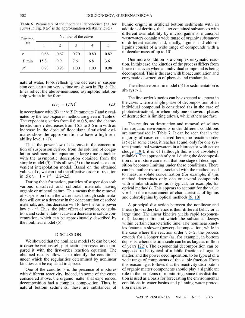
natural water. Plots reflecting the decrease in suspen-sion concentration versus time are shown in Fig. 8. Thelines reflect the above-mentioned asymptotic relation-ship written in the form

(23)

in accordance with (9) at t � T. Parameters T and ε eval-uated by the least-squares method are given in Table 6.The exponent ε varies from 0.6 to 0.8, and the charac-teristic time T decreases from 15.3 to 3.6 min with anincrease in the dose of flocculant. Statistical esti-mates show the approximation to have a high reli-ability level (~1).

Thus, the power low of decrease in the concentra-tion of suspension derived from the solution of coagu-lation–sedimentation equation at large time coincideswith the asymptotic description obtained from thesimple model (5). This allows (5) to be used as a con-venient interpolation model. Based on the obtainedvalues of ε, we can find the effective order of reactionin (5): ν = 1 + ε–1 = 2.2–2.5.

During their formation, particles of suspension sorbvarious dissolved and colloidal materials havingorganic or mineral nature. This means that the removalof suspension from the water mass through sedimenta-tion will cause a decrease in the concentration of sorbedmaterials, and this decrease will follow the same powerlaw c ~ t–ε. Thus, the joint effect of sorption, coagula-tion, and sedimentation causes a decrease in solute con-centration, which can be approximately described bythe nonlinear model (5).

DISCUSSION

We showed that the nonlinear model (5) can be usedto describe various self-purification processes and com-pared it with the first-order reaction equation. Theobtained results allow us to identify the conditions,under which the regularities determined by nonlinearkinetics can be expected to appear.

One of the conditions is the presence of mixtureswith different reactivity. Indeed, in some of the casesconsidered above, the organic matter that experienceddecomposition had a complex composition. Thus, innatural bottom sediments, these are substances of

c/c0 T /t( )ε=

humic origin; in artificial bottom sediments with anaddition of detritus, the latter contained substances withdifferent assimilability by microorganisms; municipalwastewaters contain a wide range of organic substancesof different nature; and, finally, lignins and chloro-lignins consist of a wide range of compounds with amolecular mass of up to 104.

One more condition is a complex enzymatic reac-tion. In this case, the kinetics of the process differs fromlinear one, even when an individual compound is beingdecomposed. This is the case with bioaccumulation andenzymatic destruction of phenols and rhodanides.

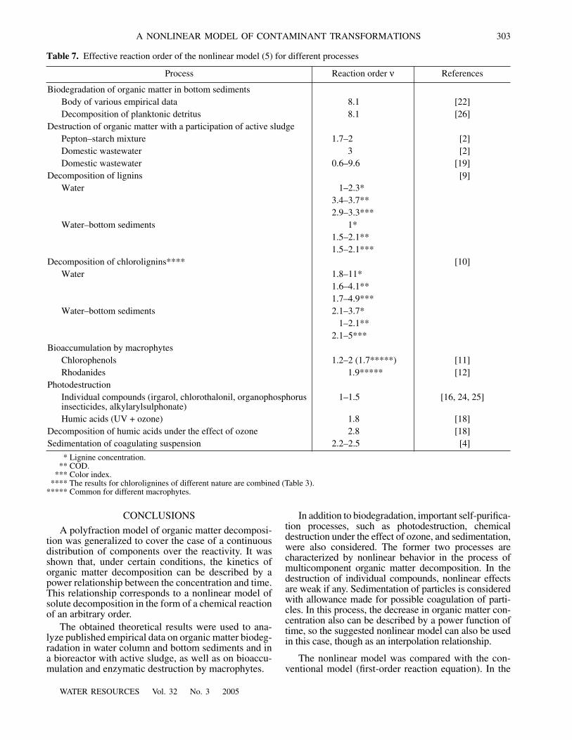
The effective order in model (5) for sedimentation isalways > 1.

The first-order kinetics can be expected to appear inthe cases where a single phase of decomposition of anindividual compound is considered (as in the case ofphotodestruction), or when only one of several phasesof destruction is limiting (slow), while others are fast.

The results on destruction and removal of solutesfrom aquatic environments under different conditionsare summarized in Table 7. It can be seen that in themajority of cases considered here, the reaction orderis >1; in some cases, it reaches 1; and, only for one sys-tem (municipal wastewaters in a bioreactor with activesludge [19]), it is <1 (although this is not absolutelyreliable). The approach of ν to 1 during the decomposi-tion of a mixture can mean that one stage of decompo-sition becomes limiting under these conditions. Therecan be another reason associated with the method usedto measure solute concentration (for example, if thismethod determines only one or several compoundswith similar structures, as is typical, for example, foroptical methods). This appears to account for the valueν = 1 in the measurement of characteristics of ligninsand chlorolignins by optical methods [9, 10].

A principal distinction between the nonlinear andlinear (first-order) kinetics is their different behavior atlarge time. The linear kinetics yields rapid (exponen-tial) decomposition, at which the substance decayswithin certain characteristic time. The nonlinear kinet-ics features a slower (power) decomposition; while inthe case where the reaction order ν > 2, the processextends for a longer time (as, for example, in bottomdeposits, where the time scale can be as large as millionof years [22]). The exponential decomposition can besupposed to be typical of a labile fraction of organicmatter, and the power decomposition, to be typical of awide range of components of the stable fraction. Fromthis reasoning it follows that the reactivity distributionof organic matter components should play a significantrole in the problems of monitoring, since this distribu-tion is used as a basis for forecasting the environmentalconditions in water basins and planning water protec-tion measures.

Table 6. Parameters of the theoretical dependence (23) forcurves in Fig. 8 (R2 is the approximation reliability level)

Parame-ter

Number of the curve

1 2 3 4 5

ε 0.66 0.67 0.70 0.80 0.82

T, min 15.3 9.9 7.6 6.8 3.6

R2 0.98 0.98 1.00 1.00 0.98

WATER RESOURCES Vol. 32 No. 3 2005

A NONLINEAR MODEL OF CONTAMINANT TRANSFORMATIONS 303

CONCLUSIONS

A polyfraction model of organic matter decomposi-tion was generalized to cover the case of a continuousdistribution of components over the reactivity. It wasshown that, under certain conditions, the kinetics oforganic matter decomposition can be described by apower relationship between the concentration and time.This relationship corresponds to a nonlinear model ofsolute decomposition in the form of a chemical reactionof an arbitrary order.

The obtained theoretical results were used to ana-lyze published empirical data on organic matter biodeg-radation in water column and bottom sediments and ina bioreactor with active sludge, as well as on bioaccu-mulation and enzymatic destruction by macrophytes.

In addition to biodegradation, important self-purifica-tion processes, such as photodestruction, chemicaldestruction under the effect of ozone, and sedimentation,were also considered. The former two processes arecharacterized by nonlinear behavior in the process ofmulticomponent organic matter decomposition. In thedestruction of individual compounds, nonlinear effectsare weak if any. Sedimentation of particles is consideredwith allowance made for possible coagulation of parti-cles. In this process, the decrease in organic matter con-centration also can be described by a power function oftime, so the suggested nonlinear model can also be usedin this case, though as an interpolation relationship.

The nonlinear model was compared with the con-ventional model (first-order reaction equation). In the

Table 7. Effective reaction order of the nonlinear model (5) for different processes

Process Reaction order ν References

Biodegradation of organic matter in bottom sedimentsBody of various empirical data 8.1 [22]Decomposition of planktonic detritus 8.1 [26]

Destruction of organic matter with a participation of active sludgePepton–starch mixture 1.7–2 [2]Domestic wastewater 3 [2]Domestic wastewater 0.6–9.6 [19]

Decomposition of lignins [9]Water 1–2.3*

3.4–3.7**2.9–3.3***

Water–bottom sediments 1*1.5–2.1**1.5–2.1***

Decomposition of chlorolignins**** [10]Water 1.8–11*

1.6–4.1**1.7–4.9***

Water–bottom sediments 2.1–3.7*1–2.1**

2.1–5***Bioaccumulation by macrophytes

Chlorophenols 1.2–2 (1.7*****) [11]Rhodanides 1.9***** [12]

PhotodestructionIndividual compounds (irgarol, chlorothalonil, organophosphorus insecticides, alkylarylsulphonate)

1–1.5 [16, 24, 25]

Humic acids (UV + ozone) 1.8 [18]Decomposition of humic acids under the effect of ozone 2.8 [18]Sedimentation of coagulating suspension 2.2–2.5 [4]

* Lignine concentration. ** COD. *** Color index. **** The results for chlorolignines of different nature are combined (Table 3).***** Common for different macrophytes.

304

WATER RESOURCES Vol. 32 No. 3 2005

DOLGONOSOV, GUBERNATOROVA

majority of cases considered, the nonlinear model bet-ter fits experimental data.

The conditions under which nonlinear effectsappear (the presence of a mixture of compounds withdifferent reactivity and a complex enzymatic reaction)are discussed.

The results of this study show that the chemical termin hydrological migration models of a reactive soluteshould be represented by the nonlinear model describedhere, rather than the commonly used first-order reactionequation.

ACKNOWLEDGMENTS

This study was supported by the Russian Founda-tion for Basic Research, project no 05–05–65241.

REFERENCES

1. Aizatullin, T.A. and Lebedev, Yu.M., Simulation ofOrganic Pollutant Transformations in Ecosystems andSelf-Purification of Water Streams and Bodies, in ItogiNauki Tekhn. Obshch. Ekol., Biotsen., Gidrobiol., Mos-cow: VINITI, 1977, vol. 4, pp. 8–74.

2. Vavilin, V.A., Nelineinye modeli biologicheskoi ochistkii protsessov samoochishcheniya v rekakh (NonlinearModels of Biological Treatment and Self-PurificationProcesses in Rivers), Moscow: Nauka, 1983.

3. Dolgonosov, B.M., Problems of Water Quality Maintain-ing in a Natural–Technological Water Supply Complex,Inzh. Ekologiya, 2003, no. 5, pp. 2–14.

4. Kul’skii, L.A., Teoreticheskie osnovy i tekhnologiya kon-ditsionirovaniya vody (Theoretical Principles and Tech-nology of Water Conditioning), Kiev: Naukova Dumka,1980.

5. Leonov, A.V. and Aizatullin, T.A., Kinetics and Mechanismof Transformation of Biophil Elements (S, O, N, P, S) inAquatic Ecosystems, in Itogi Nauki Tekhn. Obshch.Ekol., Biotsen., Gidrobiol.,, Moscow: VINITI, 1977, vol. 4,pp. 75–137.

6. Ostroumov, S.A., The Concept of Aquatic Biota as aLabile and Vulnerable Component of the Water Self-Purification System, Dokl. Akad. Nauk, 2000, vol. 372,no. 2, pp. 279–282 [Dokl. (Engl. Transl.), vol. 372, no. 2,pp. 286–289].

7. Ostroumov, S.A., Biodiversity Protection and Quality ofWater: The Role of Feedbacks in Ecosystems, Dokl.Akad. Nauk, 2002, vol. 382, no. 1, pp. 138–141 [Dokl.(Engl. Transl.), vol. 382, no. 1, pp. 18–21].

8. Paal’me, L.P., Priiman, R.E., Glushko, M.I., andGubergrits, M.Ya., Joint Photoinitiated Oxidation of 3,4-benzpyrene and Alkylarylsulphonates, Vodn. Resur.,1975, no. 2, pp. 174–178.

9. Timofeeva, S.S. and Beim, A.M., Regularities in Trans-formations of Lignin Substances in the Water of EasternSiberian Water Bodies, Vodn. Resur., 1990, no. 2,pp. 115–120.

10. Timofeeva, S.S. and Beim, A.M., Regularities of Eco-logical Transformation of Chlorolignins in NaturalWaters, Vodn. Resur., 1996, vol. 23, no. 4, pp. 467–471

[Water Resour. (Engl. Transl.), vol. 23, no. 4, pp. 435–439].

11. Timofeeva, S.S. and Beim, A.M., The Role of Macro-phytes in the Neutralization of Phenols, Vodn. Resur.,1992, no. 1, pp. 89–94.

12. Timofeeva, S.S. and Men’shikova, O.A., The Use ofMacrophytes for the Intensification of Biological Treat-ment of Rhodanide-Containing Wastewater, Vodn. Resur.,1986, no. 6, pp. 80–85.

13. Upravlenie riskom: Risk. Ustoichivoe razvitie. Sinerget-ika (Risk Control: Risk, Sustainable Development, Syn-ergetics), Moscow: Nauka, 2000.

14. Berner, R.A., A Rate Model for Organic Matter Decom-position During Bacterial Sulfate Reduction in MarineSediments, Biogeochemistry of Organic Matter at theSediment–Water Interface. CNRS Int. Colloq, 1980,pp. 35–44.

15. Fair, G.M. and Geyer, J.C., Water Supply and Wastewa-ter Disposal, New York: Wiley, 1954.

16. Harada, K., Hisanaga, T., and Tanaka, K., PhotocatalyticDegradation of Organophosphorous Insecticides inAqueous Semiconductor Suspensions, Water Res., 1990,vol. 24, no. 11, pp. 1415–1417.

17. Janssen, B.H., A Simple Method for Calculating Decom-position and Accumulation of “Young” Soil OrganicMatter, Plant Soil, 1984, vol. 76, pp. 297–304.

18. Kusakabe, K., Aso, S., Hayashi, J.-I., et al., Decomposi-tion of Humic Acid and Reduction of TrihalomethaneFormation Potential in Water by Ozone with UV Irradi-ation, Water Res., 1990, vol. 24, no. 6, pp. 781–785.

19. Liwarska-Bizukojc, E., Bizukojc, M., and Ledakowicz, S.,Kinetics of the Aerobic Biological Degradation ofShredded Municipal Solid Waste in Liquid Phase, WaterRes., 2002, vol. 36, pp. 2124–2132.

20. Lowen, S.B. and Teich, M.C., Fractal Renewal ProcessesGenerate 1/f Noise, Phys. Rev. E., 1993, vol. 47, no. 2,pp. 992–1001.

21. Maslov, S., Paczuski, M., and Bak, P., Avalanches and1/f Noise in Evolution and Growth Models, Phys. Rev.Lett., 1994, vol. 73, no. 16, pp. 2162–2165.

22. Middelburg, J.J., A Simple Rate Model for Organic Mat-ter Decomposition in Marine Sediments, Geochim. Cos-mochim. Acta, 1989, vol. 53, no. 7, pp. 1577–1581.

23. Moser, A., Kinetics of Batch Fermentations, in Biotech-nology: Bioprocesses, Rehm, H.-J. and Reed, G., Eds.,Weinheim: VCH Verlangsgesellschaft, 1985, vol. 2.

24. Sakkas, V.A., Lambropoulou, D.A., Albanis, T.A., Pho-tochemical Degradation Study of Irgarol 1051 in NaturalWaters: Influence of Humic and Fulvic Substances onthe Reaction, J. Photochem. Photobiol., A: Chem., 2002,vol. 147, pp. 135–141.

25. Sakkas, V.A., Lambropoulou, D.A., Albanis, T.A., Studyof Chlorothalonil Photodegradation in Natural Watersand in the Presence of Humic Substances, Chemosphere,2002, vol. 48, pp. 939–945.

26. Westrich, J.T. and Berner, R.A., The Role of Sedimen-tary Organic Matter in Bacterial Sulfate Reduction:The G Model Tested, Limnol. Oceanogr., 1984, vol. 29,no. 2, pp. 236–249.