Groundwater Contaminant Plume Maps and Volumes, 100-K ...
74
U.S. Department of the Interior U.S. Geological Survey Open-File Report 2016–1161 Prepared in cooperation with the U.S. Fish and Wildlife Service and the Hanford Natural Resource Trustee Council Groundwater Contaminant Plume Maps and Volumes, 100-K and 100-N Areas, Hanford Site, Washington
-
Upload
khangminh22 -
Category
Documents
-
view
1 -
download
0
Transcript of Groundwater Contaminant Plume Maps and Volumes, 100-K ...

U.S. Department of the InteriorU.S. Geological Survey
Open-File Report 2016–1161
Prepared in cooperation with the U.S. Fish and Wildlife Service and the Hanford Natural Resource Trustee Council
Groundwater Contaminant Plume Maps and Volumes,100-K and 100-N Areas, Hanford Site, Washington

Groundwater Contaminant Plume Maps and Volumes, 100-K and 100-N Areas, Hanford Site, Washington
By Kenneth H. Johnson
Prepared in cooperation with the U.S. Fish and Wildlife Service and the Hanford Natural Resource Trustee Council
Open-File Report 2016–1161
U.S. Department of the Interior U.S. Geological Survey

U.S. Department of the Interior SALLY JEWELL, Secretary
U.S. Geological Survey Suzette M. Kimball, Director
U.S. Geological Survey, Reston, Virginia: 2016
For more information on the USGS—the Federal source for science about the Earth, its natural and living resources, natural hazards, and the environment—visit http://www.usgs.gov/ or call 1–888–ASK–USGS (1–888–275–8747).
For an overview of USGS information products, including maps, imagery, and publications, visit http://store.usgs.gov/.
Any use of trade, firm, or product names is for descriptive purposes only and does not imply endorsement by the U.S. Government.
Although this information product, for the most part, is in the public domain, it also may contain copyrighted materials as noted in the text. Permission to reproduce copyrighted items must be secured from the copyright owner.
Suggested citation: Johnson, K.H., 2016, Groundwater contaminant plume maps and volumes, 100-K and 100–N Areas, Hanford Site, Washington: U.S. Geological Survey Open-File Report 2016–1161, 64 p., http://dx.doi.org/10.3133/ofr20161161.
ISSN 2331-1258 (online)

iii
Contents Abstract ...................................................................................................................................................................... 1 Introduction ................................................................................................................................................................. 2
Purpose and Scope ................................................................................................................................................. 3 Description of Study Area ....................................................................................................................................... 3
Location ............................................................................................................................................................... 3 Surficial Features ................................................................................................................................................ 5 Groundwater ........................................................................................................................................................ 5 Geology ............................................................................................................................................................... 8 Contaminants .................................................................................................................................................... 12
Hexavalent Chromium ................................................................................................................................... 18 Tritium ............................................................................................................................................................ 19 Nitrate ............................................................................................................................................................ 19 Strontium-90 .................................................................................................................................................. 20 Carbon-14 ...................................................................................................................................................... 20 Plume Overlaps ............................................................................................................................................. 20
Methods of Analysis .................................................................................................................................................. 22 Selection of Wells.................................................................................................................................................. 22 Representative Concentrations ............................................................................................................................. 22 Linearization of Concentration Distribution ............................................................................................................ 23 Spatial Interpolation of Concentrations ................................................................................................................. 28 Plume Interpretation: Area and Volume Calculations ............................................................................................ 36 Maximal and Minimal Plume Extents .................................................................................................................... 38
Results ...................................................................................................................................................................... 39 Plume Delineation ................................................................................................................................................. 39
Hexavalent Chromium ....................................................................................................................................... 56 Tritium ............................................................................................................................................................... 56 Nitrate ................................................................................................................................................................ 57 Strontium-90 ...................................................................................................................................................... 57 Carbon-14 ......................................................................................................................................................... 57
Total Quantity of Contaminated Groundwater ....................................................................................................... 57 Upper and Lower Limits ........................................................................................................................................ 57 Error Analysis ........................................................................................................................................................ 58
Limitations ................................................................................................................................................................ 60 Summary .................................................................................................................................................................. 60 References Cited ...................................................................................................................................................... 61 Appendix A. Calculation Spreadsheets for Groundwater Contaminant Plume Maps and Volumes, 100-K and 100-N Areas, Hanford Site, Washington ................................................................................................. 64

iv
Figures Figure 1. Map showing location of 100-K and 100-N study area, Hanford Site, Washington ................................... 4 Figure 2. Map showing surficial features of study area, Hanford Site, Washington ................................................. 6 Figure 3. Map showing averaged groundwater altitudes in study area, Hanford Site, Washington, 2009–12 .......... 7 Figure 4. Diagram generalized hydrogeology of study area, Hanford Site, Washington .......................................... 9 Figure 5. Map showing estimated altitude of top of Ringold Upper Mud (RUM) in study area, Hanford Site, Washington .............................................................................................................................................................. 10 Figure 6. Saturated thickness of uppermost unconfined aquifer in study area, Hanford Site, Washington ............ 11 Figure 7. Map showing plume extents of hexavalent chromium in the study area, Hanford Site, Washington ....... 13 Figure 8. Map showing plume extents of tritium in the study area, Hanford Site, Washington ............................... 14 Figure 9. Map showing plume extents of nitrate in the study area, Hanford Site, Washington ............................... 15 Figure 10. Map showing plume extents of strontium-90 in the study area, Hanford Site, Washington ................... 16 Figure 11. Map showing plume extents of carbon-14 in the study area, Hanford Site, Washington....................... 17 Figure 12. Map showing overlapping plumes for five contaminants in the study area, Hanford Site, Washington .. 21 Figure 13. Graphs showing fitted log normal probability distribution to tritium activity data in samples, Hanford Site, Washington ...................................................................................................................................................... 24 Figure 14. Graphs showing fitted log normal probability distributions for other contaminant data, Hanford Site, Washington .............................................................................................................................................................. 26 Figure 15. Map showing grid used for interpolation and blanked or unblanked from display using SURFER® application ............................................................................................................................................................... 29 Figure 16. Map showing examples of effects of different interpolation methods on tritium plume contouring in 100-K Area .............................................................................................................................................................. 30 Figure 17. Map showing U.S. Geological Survey plume extents of hexavalent chromium in the study area, Hanford Site, Washington ........................................................................................................................................ 31 Figure 18. Map showing U.S. Geological Survey plume extents of tritium in the study area, Hanford Site, Washington .............................................................................................................................................................. 32 Figure 19. Map showing U.S. Geological Survey plume extents of nitrate in the study area, Hanford Site, Washington .............................................................................................................................................................. 33 Figure 20. Map showing U.S. Geological Survey plume extents of strontium-90 in the study area, Hanford Site, Washington .............................................................................................................................................................. 34 Figure 21. Map showing U.S. Geological Survey plume extents of carbon-14 in the study area, Hanford Site, Washington .............................................................................................................................................................. 35 Figure 22. Diagram of calculation of volume of contaminated water, Hanford Site, Washington ............................ 37 Figure 23. Map showing detail of U.S. Geological Survey nitrate plumes in 100-N Area showing upper and lower limits, Hanford Site, Washington .................................................................................................................... 40 Figure 24. Maps showing hexavalent chromium plumes for average well values, upper confidence limits on well averages, and lower confidence limits on well average, Hanford Site, Washington ......................................... 41 Figure 25. Maps showing tritium plumes for average well values, upper confidence limits on well averages, and lower confidence limits on well averages, Hanford Site, Washington ............................................................... 44 Figure 26. Maps showing nitrate plumes for average well values, upper confidence limits on well averages, and lower confidence limits on well averages, Hanford Site, Washington ............................................................... 47 Figure 27. Maps showing strontium-90 plumes for average well values, upper confidence limits on well averages, and lower confidence limits on well averages, Hanford Site, Washington. .............................................. 50 Figure 28. Maps showing carbon-14 plumes for average well values, confidence limits on well averages, and lower confidence limits on well averages, Hanford Site, Washington ...................................................................... 53

v
Tables Table 1. Areas of plumes, 100-N and 100-K Areas, Hanford Site, Washington ...................................................... 12 Table 2. Volumes of contaminated groundwater in plumes, 100-K and 100K-N Areas, Hanford Site, Washington ............................................................................................................................................................. 37 Table 3. Differences in contaminant plume volume for extreme extents compared to average plume extents, Hanford Site, Washington ........................................................................................................................................ 58
Conversion Factors International System of Units to Inch/Pound
Multiply By To obtain
Length millimeter (mm) 0.03937 inch (in.)
meter (m) 3.281 foot (ft)
meter (m) 1.094 yard (yd)
kilometer (km) 0.6214 mile (mi)
Area
square meter (m2) 0.0002471 acre
square meter (m2) 10.76 square foot (ft2)
square kilometer (km2) 247.1 acre
square kilometer (km2) 0.3861 square mile (mi2)
Volume cubic meter (m3) 264.2 gallon (gal)
liter (L) 1.057 quart (qt)
liter (L) 0.2642 gallon (gal)
liter (L) 61.02 cubic inch (in3)
cubic centimeter (cm3) 0.06102 cubic inch (in3)
cubic decimeter (dm3) 61.02 cubic inch (in3)
cubic meter (m3) 35.31 cubic foot (ft3)
cubic meter (m3) 1.308 cubic yard (yd3)
cubic meter (m3) 0.0008107 acre-foot (acre-ft)
Mass
gram (g) 0.03527 ounce, avoirdupois (oz)
kilogram (kg) 2.205 pound avoirdupois (lb)
Hydraulic gradient
meter per kilometer (m/km) 5.27983 foot per mile (ft/mi)

vi
Inch/Pound to International System of Units
Multiply By To obtain
Radioactivity
picocurie per liter (pCi/L) 0.037 becquerel per liter (Bq/L)
Supplemental Information Temperature in degrees Celsius (°C) may be converted to degrees Fahrenheit (°F) as
°F = (1.8 × °C) + 32.
Temperature in degrees Fahrenheit (°F) may be converted to degrees Celsius (°C) as
°C = (°F – 32) / 1.8.
Concentrations of chemical constituents in water are given in either milligrams per liter (mg/L) or micrograms per liter (µg/L).
Activities for radioactive constituents in water are given in picocuries per liter (pCi/L).
Datums Vertical coordinate information is referenced to the North American Vertical Datum of 1988 (NAVD 88), referred to in this report as “sea level.”
Horizontal coordinate information is referenced to the North American Datum of 1983 (NAD 83).
Altitude, as used in this report, refers to distance above or below sea level.
Abbreviations CDF Cumulative Probability Distribution Function
CERCLA Comprehensive Environmental Response, Compensation, and Liability Act
DEM Digital Elevation Model
DOI U.S. Department of the Interior
EPA U.S. Environmental Protection Agency
GIS Geographic Information Systems
HNRTC Hanford Natural Resource Trustee Council
LWDF Liquid Waste Disposal Facility
MCL Maximum Contaminant Level (drinking water standard)
NAIP National Agricultural Imagery Program
NRDA Natural Resource Damage Assessment
RUM Ringold Upper Mud geologic unit
TWG [Groundwater] Technical Working Group, a subgroup of HNRTC
USDA U.S. Department of Agriculture
DOE U.S. Department of Energy
USGS U.S. Geological Survey
1
Groundwater Contaminant Plume Maps and Volumes, 100-K and 100-N Areas, Hanford Site, Washington
By Kenneth H. Johnson
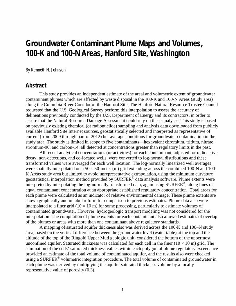
Abstract This study provides an independent estimate of the areal and volumetric extent of groundwater
contaminant plumes which are affected by waste disposal in the 100-K and 100-N Areas (study area) along the Columbia River Corridor of the Hanford Site. The Hanford Natural Resource Trustee Council requested that the U.S. Geological Survey perform this interpolation to assess the accuracy of delineations previously conducted by the U.S. Department of Energy and its contractors, in order to assure that the Natural Resource Damage Assessment could rely on these analyses. This study is based on previously existing chemical (or radionuclide) sampling and analysis data downloaded from publicly available Hanford Site Internet sources, geostatistically selected and interpreted as representative of current (from 2009 through part of 2012) but average conditions for groundwater contamination in the study area. The study is limited in scope to five contaminants—hexavalent chromium, tritium, nitrate, strontium-90, and carbon-14, all detected at concentrations greater than regulatory limits in the past.
All recent analytical concentrations (or activities) for each contaminant, adjusted for radioactive decay, non-detections, and co-located wells, were converted to log-normal distributions and these transformed values were averaged for each well location. The log-normally linearized well averages were spatially interpolated on a 50 × 50-meter (m) grid extending across the combined 100-N and 100-K Areas study area but limited to avoid unrepresentative extrapolation, using the minimum curvature geostatistical interpolation method provided by SURFER® data analysis software. Plume extents were interpreted by interpolating the log-normally transformed data, again using SURFER®, along lines of equal contaminant concentration at an appropriate established regulatory concentration . Total areas for each plume were calculated as an indicator of relative environmental damage. These plume extents are shown graphically and in tabular form for comparison to previous estimates. Plume data also were interpolated to a finer grid (10 × 10 m) for some processing, particularly to estimate volumes of contaminated groundwater. However, hydrogeologic transport modeling was not considered for the interpolation. The compilation of plume extents for each contaminant also allowed estimates of overlap of the plumes or areas with more than one contaminant above regulatory standards.
A mapping of saturated aquifer thickness also was derived across the 100-K and 100–N study area, based on the vertical difference between the groundwater level (water table) at the top and the altitude of the top of the Ringold Upper Mud geologic unit, considered the bottom of the uppermost unconfined aquifer. Saturated thickness was calculated for each cell in the finer (10 × 10 m) grid. The summation of the cells’ saturated thickness values within each polygon of plume regulatory exceedance provided an estimate of the total volume of contaminated aquifer, and the results also were checked using a SURFER® volumetric integration procedure. The total volume of contaminated groundwater in each plume was derived by multiplying the aquifer saturated thickness volume by a locally representative value of porosity (0.3).

2
Estimates of the uncertainty of the plume delineation also are presented. “Upper limit” plume delineations were calculated for each contaminant using the same procedure as the “average” plume extent except with values at each well that are set at a 95-percent upper confidence limit around the log-normally transformed mean concentrations, based on the standard error for the distribution of the mean value in that well; “lower limit” plumes are calculated at a 5-percent confidence limit around the geometric mean. These upper- and lower-limit estimates are considered unrealistic because the statistics were increased or decreased at each well simultaneously and were not adjusted for correlation among the well distributions (i.e., it is not realistic that all wells would be high simultaneously). Sources of the variability in the distributions used in the upper- and lower-extent maps include time varying concentrations and analytical errors.
The plume delineations developed in this study are similar to the previous plume descriptions developed by U.S. Department of Energy and its contractors. The differences are primarily due to data selection and interpolation methodology. The differences in delineated plumes are not sufficient to result in the Hanford Natural Resource Trustee Council adjusting its understandings of contaminant impact or remediation.
Introduction The Hanford Site in south-central Washington, managed by the U.S. Department of Energy
(DOE), was established in 1943 to produce nuclear materials for national defense as part of the top secret Manhattan Project (U.S. Department of Energy, 2016). Many of these activities produced waste that contain radioactive materials and hazardous contaminants, some of these waste materials were disposed as liquids into the ground. These disposed wastes have contaminated large volumes of groundwater across the Hanford Site. All the production facilities, which included nine nuclear reactors and associated processing facilities, are now closed. Work is underway to clean up the waste and contamination that is a legacy of these nuclear operations.
Along with the agencies involved in the cleanup work, various Federal, State, and Tribal governments act as natural resource trustees for resources associated with the Hanford Site under the Natural Resource Damage Assessment (NRDA) provisions of the Comprehensive Environmental Response, Compensation, and Liability Act (CERCLA). The Hanford Natural Resource Trustee Council (HNRTC) includes: the DOE, the U.S. Department of the Interior (DOI) through U.S. Fish and Wildlife Service and the U.S. Department of Commerce through the National Oceanic Atmospheric Administration; the States of Washington and Oregon; and the Confederated Tribes and Bands of the Yakama Nation, the Confederated Tribes of the Umatilla Indian Reservation and the Nez Perce Tribe. The HNRTC is responsible for ensuring the public’s natural resources are protected and conserved throughout the cleanup process and that the public is made whole by restoration of injured natural resources resulting from the release of hazardous substances through the NRDA process of CERCLA. The HNRTC has developed an Injury Assessment Plan (Hanford Natural Resource Trustees, 2013) as part of the NRDA process for the Hanford Site, with the objective of better integration of natural resource concerns, including those for groundwater, into ongoing response actions at the Hanford Site.
The HNRTC perceived a need to fill information gaps identified to be crucial for the injury assessment plan. One of these possible gaps is the adequacy of the groundwater contaminant plume maps as generated by DOE and its contractors.

3
Purpose and Scope This study is designed to develop independent estimates of groundwater contaminant plumes on
the Hanford Site, to allow comparison with those published by the DOE. This will assist the HNRTC to institute appropriate mitigation measures for the contamination.
The scope includes only the adjacent 100-K and 100-N Areas, which together extend more than 5 km along the Columbia River (fig. 1). The polygon outlines of the two areas that are used in this report were obtained from groundwater spatial data from the Environmental Dashboard Application (CH2M Hill, 2012a) as groundwater interest areas (“GwInterestAreas_2008”, designated there as “100-KR-4” and “100-NR-2”). The combined areal extent is referred to here as the study area. Some analysis was extended beyond the study area to include the information from wells farther upgradient, and the extent also was adjusted to omit portions that lie beneath the Columbia River because data are absent in this area.
The analysis in this report includes five contaminants of concern that have been detected in groundwater—hexavalent chromium, tritium, nitrate, strontium-90, and carbon-14. Data for these contaminants were downloaded from Hanford Site reports (Rieger, 2012). The DOE graphical plume extents also were obtained from the “Environmental Dashboard Application” (CH2M Hill, 2012a) to allow graphical comparison to the new estimates presented in this report. Note that although some of the contaminants are radionuclides and some are chemical contaminants, for simplicity in this report, the term “concentration” is used here generically to also include activity when referring to both chemical constituents and radionuclides.
This analysis uses sampling and analytical data primarily from a 3-year period (2009–11 inclusive, plus part of 2012) to provide sufficient data for statistical analysis and at the same time be representative of present day groundwater contamination. When a well did not have data for 2009–12, data from the most recent 3-year period that did have sufficient data were included, decayed to 2009–12 values according to the half-life for a radionuclide. The analysis regards only contamination in saturated groundwater and does not include any contamination presently partitioned in disposal facilities, adsorbed to soil, or in the vadose zone above the saturated aquifer.
Description of Study Area To provide context for the study, the following sections describe the study location, surficial
features, geology, groundwater, and the nature of the contaminants that were studied.
Location The Hanford Site is located mostly in Benton County in southcentral Washington near Richland,
adjacent to the Columbia River (fig. 1). The 1,518-km2 Hanford Site, administered by the DOE, has a semiarid shrub-steppe climate with normal annual precipitation about 177 mm, and average monthly temperatures ranging from about 0 °C in January to 25° C in July (Hoitink and others, 2005).
The 100-K and 100-N Areas are 12.8 and 6.4 km2 in size, respectively (CH2M Hill, 2012a). As mentioned above, because there is no information of conditions beneath the Columbia River, the study area is restricted to the land portion of the two areas, cut off at the approximate bank of the river. With this adjustment the study area is approximately 17.9 km2.

4
Figure 1. Map showing location of 100-K and 100-N study area, Hanford Site, Washington.

5
Surficial Features During operational phase for the Hanford Site (1943–88), the study area contained plutonium
production reactors (105-KW, 105-KE, and 105-N), and several associated liquid waste disposal facilities (LWDF), including cribs1, basins, and trenches. Selected historical facilities are shown in figure 2, including those identified as probable major contributors to groundwater contamination (U.S. Department of Energy, 2012b). Since the 1988 end of the operational phase of the reactors, some additional contamination may have been transported into the local groundwater from contaminated sites upgradient of the study area or downward from the overlying vadose zone, while some previous contamination has diminished due to decay or transport offsite into the Columbia River. The study area also has hosted a number of remediation projects in recent years, which have altered the distribution of contamination by removing constituents, immobilizing them, or displacing them by injection of clean water. The analysis for the present study attempts to show the extent of contamination based on samples obtained between January 2009 through about April 2012.
The figures in this report include a background image from the National Agricultural Imagery Program (NAIP; U.S. Department of Agriculture, 2006) to provide landmarks for reference. The NAIP shows roads, structures, and land disturbance from previous excavations at a 1-m resolution. Contours of land-surface altitude shown in figure 2 are based on the Washington Digital Elevation Model (U.S. Geological Survey, 2000) which has a resolution of 30 m. The DEM ground-surface altitude in the study area averages approximately 147.5 m, and ranges from 117.8 m (altitude along the Columbia River bank) to 164.8 m near the southern boundary of the 100-K Area.
Groundwater Contours of estimated recent (2009–12) groundwater levels (potentiometric surface altitudes) in
the near-surface unconfined aquifer are shown in figure 3, based on averages of the water-level measurements in wells during this time frame. The average altitude of this estimated water table in the study area is 120.3 m, and ranges from 117.6 m at the Columbia River to 121.9 m inland. The general groundwater-flow direction in the study area is from south to north, then bending northwest to flow directly into the Columbia River. Near the Columbia River, the gradient adjusts slightly to accord with the surface-water gradient in the river as it flows to the northeast. The Columbia River has a typical stage (surface altitude) in this area of about 118 m and a gradient of approximately 0.23 m per river km (Waichler and others, 2005), therefore the river stage decreases about 1.2 m along the 5-km length of the edge of the study area. During sub-annual time scales, the stage in the Columbia River (and similarly the groundwater altitude near it) rises or declines depending on the flow of water released from the Priest Rapids Dam for hydroelectric power about 10 km upstream (fig. 1). The daily average gage height at the U.S. Geological Survey (USGS) streamgage 12472800 on the Columbia River just downstream of the dam (fig. 1) ranged from 2.04 to 9.00 m during the 2009–12 study period (U.S. Geological Survey, 2012). This reach is one of the few remaining free-flowing sections of the Columbia River.
1 “A crib is an underground structure designed to allow liquid wastes to percolate to the soil.” (Lichtenstein, 2004, p.811)

6
Figure 2. Map showing surficial features of study area, Hanford Site, Washington.

7
Figure 3. Map showing averaged groundwater altitudes (in meters above North American Vertical Datum of 1988) in study area, Hanford Site, Washington, 2009–12.

8
There are a several locations in the study area where groundwater levels are anomalously higher or lower than the general trend; these appear to be attributable to injection or extraction (production) wells for remedial pump and treat or barrier placement systems (Ivarson and others, 2012). With these remedial actions, in addition to the effects of the Columbia River, groundwater altitudes in the study area are dynamic. Because of these complications, the present study did not include the effects of groundwater transport on plume direction and extent.
During the operational phase, large quantities of wastewater were disposed of in the Central Plateau area (200-E and 200-W Areas) of the Hanford Site (fig. 1), as well as locally in the 100 Areas, which includes the study area. This disposal practice raised groundwater levels, changed gradients, and altered natural groundwater flow directions, in addition to creating contaminant plumes. The groundwater-flow prior to the development of the Hanford Site was oriented from northwest to southeast across the Hanford Site from the Columbia River and back (U.S. Department of Energy, 1992). During the remediation phase in the Hanford Site, groundwater levels and gradients have been greatly reduced and the flow system has nearly reverted to pre-development conditions. For example, in some wells just south of the study area perimeter (for example, wells 699-77-54 and 699-70-68, fig. 3) water levels have declined about 3 m from their highest levels in 1969–70. To put this into perspective, this change in water level is approximately the same as the range of present day (2009–2012) average groundwater levels across the entire study area (fig. 3).
Geology The general geology of the Hanford Site is Columbia River Basalts overlain by the Ringold
Formation, a primarily fine-grained fluvial sedimentary unit, and in turn overlain by the Hanford Formation, a glacial flood deposit, near the ground surface (fig. 4, reproduced from Hartman, 2012). The basalts are deep, with their top at about sea level in the study area, so these basalts are recorded in well logs of only a few of the deeper wells. In the study area, the uppermost portion of the Ringold Formation is the Ringold Unit E, a fluvial sand and gravel, which is generally the unconfined aquifer. Underlying Unit E, but still in the Ringold Formation, is a fine-grained material referred to as the Ringold Upper Mud (RUM). The RUM serves as an confining unit and forms the bottom of the local unconfined aquifer in the Ringold Unit E. Using the altitudes where various wells across the study area are reported to intersect the RUM, a map of the altitude of the top of the RUM was developed (fig. 5). The altitude of this top of the RUM averages about 102 m across the study area, and extends between 86 and 117 m. The top of the RUM is generally higher in the northeast (in the 100-N Area) and slopes down to the southwest, although there appears to be an isolated high point in the center of the 100-K Area near well 199-K-128 (fig. 5) and confirmed by high levels in a couple of other nearby wells. These estimates of top of the RUM also were checked against wells that were drilled but did not reach the RUM, and the data for these wells agreed with the interpolation based on the wells that did intersect the RUM (that is, the bottoms of the non-intersected wells were higher in altitude than the top of the RUM).
Overlying the Ringold Formation is the Hanford Formation, a primarily glacial flood outwash deposit, and some fill material near the ground surface. The reported altitude of the bottom of the Hanford Formation was also checked at each well to determine whether the local water table was high enough to intrude the Hanford Formation; fewer than 10 percent of the local wells indicated that groundwater extends into the Hanford Formation, and in most of those wells the water table was less than 1 m into the Hanford Formation. The unconfined unit in the study area is therefore almost completely in the Ringold Unit E, bounded at its bottom by the RUM.

9
The (vertical) altitude difference between the water table (fig. 3) and the top of the RUM (fig. 5) is the thickness of the saturated zone of the uppermost unconfined aquifer (fig. 6). Because of the greater range of values (about 31 m) for the top altitude of the RUM compared to the range of altitudes of the water table (4 m), the saturated thickness is mainly determined by the stratigraphy. The average saturated thickness of the aquifer in the study area is 18.8 m and ranges from 2.8 to 32.8 m.
Figure 4. Diagram generalized hydrogeology of study area, Hanford Site, Washington (from Hartman [2012]).

10
Figure 5. Map showing estimated altitude (in meters above North American Vertical Datum of 1988) of top of Ringold Upper Mud (RUM) in study area, Hanford Site, Washington.

11
Figure 6. Saturated thickness of uppermost unconfined aquifer in study area, Hanford Site, Washington.

12
Contaminants Previous analyses of groundwater quality in the study area by DOE and its contractors have
indicated the presence of several radioactive and hazardous contaminants that are at concentrations greater than regulatory limits. According to the scope of this project, these were limited to five contaminants of concern— hexavalent chromium, tritium, nitrate, strontium-90, and carbon-14.
Background information for these contaminants is presented in this section, including sources of the contaminants, regulatory limits used in the plume delineation, transport characteristics and previous remedial efforts, and plumes as delineated by the DOE or its contractors. Areas of the plumes are introduced here, shown in figures 7–11, and summarized in table 1.
The plume delineations discussed in the following sections show all the plume extents included in the graphical data from the Environmental Dashboard Application (CH2M Hill, 2012a) through the menu items “GIS Data / Groundwater Spatial Data / Groundwater Report 2010 / Download.” These graphics include lines of equal concentration for values that are higher or lower than the regulatory limits, as well as plumes that may be near or even cross the study area, but come from other sources and show up in wells outside of the study area. The wells that are shown in figures 7–11 also are from shapefiles in the graphics download (CH2M Hill, 2012a).
Table 1. Areas of plumes, 100-N and 100-K Areas, Hanford Site, Washington. [MCL or equivalent concentration: MCL, Maximum Concentration Level; mg/L, milligram per liter, μg/L, microgram per liter; pCi/L, picocuries per liter. USGS plumes: Area of contaminant plumes delineated by U.S. Geological Survey (USGS), in square kilometers. DOE plumes: Area of contaminant plumes delineated by U.S. Department of Energy (DOE), in square kilometers]
Contaminant MCL or equivalent concentration
USGS plumes DOE plumes 100-K 100-N Total 100-K 100-N Total
Hexavalent chromium 48 µg/L 0.682 0.058 0.741 0.317 0.011 0.328 Tritium 20,000 pCi/L 0.138 0.041 0.179 0.164 0.034 0.198 Nitrate 45 mg/L 0.245 0.229 0.474 0.142 0.570 0.712 Strontium-90 8 pCi/L 0.044 0.488 0.532 0.040 0.580 0.620 Carbon-14 2,000 pCi/L 0.078 0.000 0.078 0.059 0.000 0.059

13
Figure 7. Map showing plume extents of hexavalent chromium in the study area, Hanford Site, Washington (from CH2M Hill, 2012a).

14
Figure 8. Map showing plume extents of tritium in the study area, Hanford Site, Washington (from CH2M Hill, 2012a).

15
Figure 9. Map showing plume extents of nitrate in the study area, Hanford Site, Washington (from CH2M Hill, 2012a).

16
Figure 10. Map showing plume extents of strontium-90 in the study area, Hanford Site, Washington (from CH2M Hill, 2012a).

17
Figure 11. Map showing plume extents of carbon-14 in the study area, Hanford Site, Washington (from CH2M Hill, 2012a).

18
Hexavalent Chromium Hexavalent chromium contamination in the study area resulted from disposal or spillage of
reactor cooling water that contained chromate chemicals mixed in for conditioning (Ivarson and others, 2012). There were significant discharges of this cooling water to facilities such as the 100-K Crib, the 100-K Mile Long Trench (fig. 2), and some higher concentration spillages in the 100-K Area. So much water was discarded (for example, 3 × 10¹¹ L just to the 100-K Mile Long Trench; U.S. Department of Energy, 2012b) that a groundwater mound developed and contamination spread inland, in directions that are upgradient. The chromate-contaminated cooling water releases in the 100-N Area were much less concentrated (Alexander and Hartman, 2012) which was subsequently displaced by other releases, so that the concentrations in this area are not as high. Hexavalent chromium also can be released naturally from weathering of basalt (Oze and others, 2007), a geologic material that occurs with great thickness below the entire Hanford Site. Naturally-occurring hexavalent chromium has been detected in various locations around the world at concentrations up to 73 µg/L (Oze and others, 2007), which is greater than the limiting value used in this study but these extreme values are still much less than the highest levels occurring in the study area, so naturally occurring hexavalent chromium is unlikely to be the explanation for the plumes.
The hexavalent form of chromium has been specifically investigated in this study because of its toxicity. There was no U.S. Environmental Protection Agency (EPA) Drinking Water Standard (Maximum Contaminant Level [MCL]) specifically for hexavalent chromium at the time of this project. In March 2014, the EPA finalized an MCL of 10 µg/L. However, because the previous DOE analyses used a groundwater cleanup standard of 48 µg/L for plume delineation, this same 48 µg/L limit has been used in the present study, for the purpose of comparability. Hexavalent chromium species are typically more soluble than trivalent chromium species (the other major redox state) (U.S. Environmental Protection Agency, 2000), and so most chromium measured in the groundwater (whether in filtered samples or total) is in the hexavalent form. Hexavalent chromium has been actively remediated in the 100-K Area using pump and treat systems (Foss and Charboneau, 2011).
The DOE hexavalent chromium contaminant plumes are shown in figure 7; there are six segments of plumes at concentrations greater than 48 µg/L, and 18 wells in the study area that had chromium values greater than this limit when sampled in 2010, with a maximum concentration of 630 µg/L in well 199-K-173 (fig. 7). The six plumes total to an area of 0.328 km2, with about 97 percent of the plume in the 100-K Area.
Note that the hexavalent chromium plume data available from DOE (Rieger, 2012) showed only five plumes in the study area. In reviewing the data for this investigation, an omission was discovered. The plume graphical data include line (arc) shapes for lines of equal hexavalent chromium for concentrations of 10, 20, 48, 100, and 1,000 µg/L and polygon shapefiles of plume extents for exceedances of the same values. However, in one area of 100-K downgradient (north) of the 105-N/109-N Reactor Building and along the western edge of the 107-KE Retention Basins (fig. 2), there are polylines for 10 and 20 µg/L, and a plume polygon for 100 µg/L, but no shapefile (line or plume polygon) for the intermediate 48 µg/L MCL value used in this study. A 48 µg/L plume segment was estimated by log-linear interpolation between the 20 and 100 µg/L lines obtained from Rieger (2012) and is included in the calculations and in figure 7.

19
Tritium Tritium (3H) contamination is in the form of tritiated (heavy) water from irradiation by reactor
fuel rods, either inside the reactors or in fuel storage basins (Alexander and Hartman, 2012; Ivarson and others, 2012). This waste water was discharged to the groundwater through facilities such as the 1301-N and 1325-N LWDFs, the 100-K-1 crib and the 100-K Mile Long Trench, and other cribs near the KW and KE reactors (fig. 2).
Tritium has a half-life of 12.32 years. The MCL for beta emitter radionuclides like tritium is 4 millirems per year, which for tritium in water is considered equivalent to 20,000 picocuries per liter (pCi/L) (U.S. Environmental Protection Agency 2014). The tritiated groundwater has almost identical characteristics to normal (light) water, so it intermingles and flows along with other water. Tritium is not being actively remediated in the study area.
The tritium contaminant plumes estimated by DOE are shown in figure 8. The total area of these four plume segments is calculated by geographic information system (GIS) methods to be 0.198 km2, 83 percent of the contaminated area is again in the 100-K Area. There were eight wells in the study area sampled in 2010 that had tritium values greater than the MCL, with a maximum tritium activity of 160,000 pCi/L in well 199-K-30 (fig. 8).
Nitrate Nitrate (NO3) contamination apparently resulted from disposal of condensate from ammonia-
contaminated reactor gas or possibly from septic systems (Ivarson and others, 2012). In other areas of the Hanford Site, nitrate plumes result from discharges of nitric acid that had been used for spent fuel processing for plutonium or other radionuclides. Some nitrate in other areas of the Hanford Site subsurface has been found to result from natural sources such as caliche or biological activity (Singleton and others, 2005) although it is not known if any of these processes are applicable to the study area. Nitrate may be transformed by biological activity into other forms, including being lost to the atmosphere as gaseous nitrogen.
The MCL for nitrate is 10 mg/L as reported on a nitrogen basis (as is commonly specified); the concentration data used here is measured as nitrate rather than as nitrogen so the MCL is 45 mg/L as nitrate. Nitrate has low sorption characteristics so it flows with the other groundwater (Serne, 2007) but it can readily change chemical form; so nitrate is not considered a conservative constituent in groundwater.
Nitrate plumes, as delineated by DOE at 45 mg/L MCL, are shown in figure 9 with wells sampled in 2010. There were exceedances of the MCL in 32 groundwater wells (including aquifer tubes2 in the study area (reaching a maximum nitrate concentration of 400 mg/L in well 199-N-67, fig. 9). The total area of the five segments of plumes is calculated to be 0.712 km2, with 80 percent in the 100-N Area.
2 An aquifer tube is a “(g)roundwater monitoring site installed along the river shoreline. Generally consists of a small diameter tube (less than one inch) and screen installed using push technology near the water table.” (CH2M Hill, 2012a, p. 1, https://ehs.hanford.gov/eda/textreport/openfile?title=GIS/HanfordWells_Spatial_Summary.pdf)
20
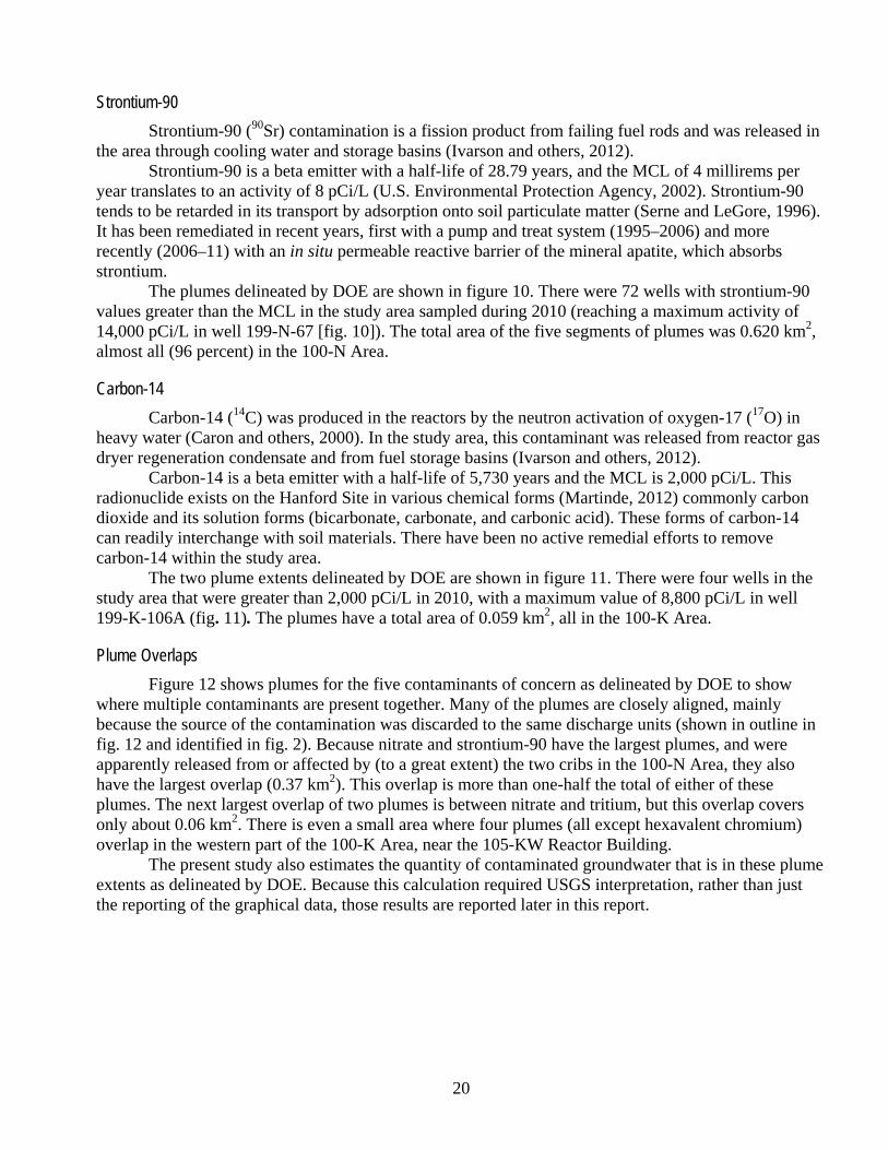
Strontium-90 Strontium-90 (90Sr) contamination is a fission product from failing fuel rods and was released in
the area through cooling water and storage basins (Ivarson and others, 2012). Strontium-90 is a beta emitter with a half-life of 28.79 years, and the MCL of 4 millirems per
year translates to an activity of 8 pCi/L (U.S. Environmental Protection Agency, 2002). Strontium-90 tends to be retarded in its transport by adsorption onto soil particulate matter (Serne and LeGore, 1996). It has been remediated in recent years, first with a pump and treat system (1995–2006) and more recently (2006–11) with an in situ permeable reactive barrier of the mineral apatite, which absorbs strontium.
The plumes delineated by DOE are shown in figure 10. There were 72 wells with strontium-90 values greater than the MCL in the study area sampled during 2010 (reaching a maximum activity of 14,000 pCi/L in well 199-N-67 [fig. 10]). The total area of the five segments of plumes was 0.620 km2, almost all (96 percent) in the 100-N Area.
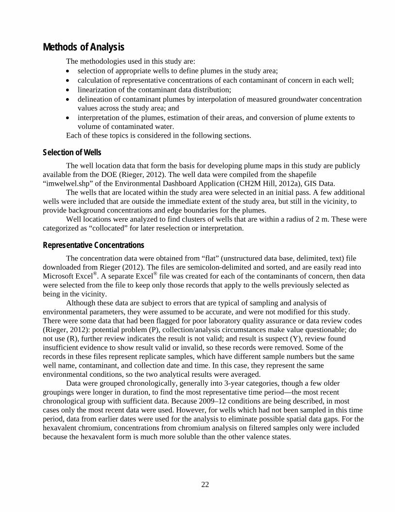
Carbon-14 Carbon-14 (14C) was produced in the reactors by the neutron activation of oxygen-17 (17O) in
heavy water (Caron and others, 2000). In the study area, this contaminant was released from reactor gas dryer regeneration condensate and from fuel storage basins (Ivarson and others, 2012).
Carbon-14 is a beta emitter with a half-life of 5,730 years and the MCL is 2,000 pCi/L. This radionuclide exists on the Hanford Site in various chemical forms (Martinde, 2012) commonly carbon dioxide and its solution forms (bicarbonate, carbonate, and carbonic acid). These forms of carbon-14 can readily interchange with soil materials. There have been no active remedial efforts to remove carbon-14 within the study area.
The two plume extents delineated by DOE are shown in figure 11. There were four wells in the study area that were greater than 2,000 pCi/L in 2010, with a maximum value of 8,800 pCi/L in well 199-K-106A (fig. 11). The plumes have a total area of 0.059 km2, all in the 100-K Area.
Plume Overlaps Figure 12 shows plumes for the five contaminants of concern as delineated by DOE to show
where multiple contaminants are present together. Many of the plumes are closely aligned, mainly because the source of the contamination was discarded to the same discharge units (shown in outline in fig. 12 and identified in fig. 2). Because nitrate and strontium-90 have the largest plumes, and were apparently released from or affected by (to a great extent) the two cribs in the 100-N Area, they also have the largest overlap (0.37 km2). This overlap is more than one-half the total of either of these plumes. The next largest overlap of two plumes is between nitrate and tritium, but this overlap covers only about 0.06 km2. There is even a small area where four plumes (all except hexavalent chromium) overlap in the western part of the 100-K Area, near the 105-KW Reactor Building.
The present study also estimates the quantity of contaminated groundwater that is in these plume extents as delineated by DOE. Because this calculation required USGS interpretation, rather than just the reporting of the graphical data, those results are reported later in this report.

21
Figure 12. Map showing overlapping plumes for five contaminants in the study area, Hanford Site, Washington (from CH2M Hill, 2012a).
22
Methods of Analysis The methodologies used in this study are: • selection of appropriate wells to define plumes in the study area; • calculation of representative concentrations of each contaminant of concern in each well; • linearization of the contaminant data distribution; • delineation of contaminant plumes by interpolation of measured groundwater concentration
values across the study area; and • interpretation of the plumes, estimation of their areas, and conversion of plume extents to
volume of contaminated water. Each of these topics is considered in the following sections.
Selection of Wells The well location data that form the basis for developing plume maps in this study are publicly
available from the DOE (Rieger, 2012). The well data were compiled from the shapefile “imwelwel.shp” of the Environmental Dashboard Application (CH2M Hill, 2012a), GIS Data.
The wells that are located within the study area were selected in an initial pass. A few additional wells were included that are outside the immediate extent of the study area, but still in the vicinity, to provide background concentrations and edge boundaries for the plumes.
Well locations were analyzed to find clusters of wells that are within a radius of 2 m. These were categorized as “collocated” for later reselection or interpretation.
Representative Concentrations The concentration data were obtained from “flat” (unstructured data base, delimited, text) file
downloaded from Rieger (2012). The files are semicolon-delimited and sorted, and are easily read into Microsoft Excel®. A separate Excel® file was created for each of the contaminants of concern, then data were selected from the file to keep only those records that apply to the wells previously selected as being in the vicinity.
Although these data are subject to errors that are typical of sampling and analysis of environmental parameters, they were assumed to be accurate, and were not modified for this study. There were some data that had been flagged for poor laboratory quality assurance or data review codes (Rieger, 2012): potential problem (P), collection/analysis circumstances make value questionable; do not use (R), further review indicates the result is not valid; and result is suspect (Y), review found insufficient evidence to show result valid or invalid, so these records were removed. Some of the records in these files represent replicate samples, which have different sample numbers but the same well name, contaminant, and collection date and time. In this case, they represent the same environmental conditions, so the two analytical results were averaged.
Data were grouped chronologically, generally into 3-year categories, though a few older groupings were longer in duration, to find the most representative time period—the most recent chronological group with sufficient data. Because 2009–12 conditions are being described, in most cases only the most recent data were used. However, for wells which had not been sampled in this time period, data from earlier dates were used for the analysis to eliminate possible spatial data gaps. For the hexavalent chromium, concentrations from chromium analysis on filtered samples only were included because the hexavalent form is much more soluble than the other valence states.

23
For the radioactive contaminants tritium and strontium-90, activity data from earlier sampling was converted to 2009–12 activity in the groundwater according to the half-life of the contaminant (12.32 and 28.79 years, respectively) and the time since sampling. Carbon-14 has a very long half-life (5,730 years) so the data for this contaminant were not adjusted for “time since sampling”. Nitrate and hexavalent chromium can change chemically over time into other species but the rates are not predictable so no adjustment was made for concentrations sampled at earlier times.
The data, as selected and processed, are presented in appendix A.
Linearization of Concentration Distribution Once the appropriate data were selected, all the values for each well were converted into an
average (interpolation value) that takes into account non-detection values and the non-linearity of the contaminant distribution. The methodology that was used to develop the lines of equal contaminant concentration included the following steps:(1) develop a log-normal probability distribution that replaces non-detect values with a representative concentration and linearizes the data for each contaminant;(2) calculate averages of log-transformed concentration data (that is, geometric mean of the original data) for each well; and(3) eliminate non-representative (low concentration) wells which are co-located with wells that have high concentrations.
The log-normal probability distribution function for each constituent dataset was prepared with the method of regression on order statistics (ROS), also referred to as the Robust (probability plot) method (Helsel and Hirsch, 2002). The following discussion is demonstrated in figure 13, using the tritium data. Data for all wells during their most recent available time period (including non-detect values at their reported sample detection limit) are shown in figure 13A in the familiar bell curve presentation. The fraction of the total number of samples (n = 1,722) in each range (bin) of activities is plotted vertically, against the activity reported horizontally at the bin’s midpoint on a log scale. Reported values for both non-detections and detections are shown, each with its own bell curve, and also a curve for all samples. Note that for tritium, there are samples (75, or 4.3 percent of the total samples) with reported activities that are negative, even though this is physically impossible. This occurs because of the way that uncertainty in analysis for radionuclide activity is taken into consideration in reporting results.
Figure 13B shows the cumulative probability distribution function (CDF) for the same data, which plots the fraction of samples with values less than or equal to a given bin value, rather than just the fraction in the bin. For clarity in presentation, “non-detection only’ plot is plotted according to the total number of non-detections, n = 366, rather than the count for all the samples, n = 1,722, and as a result reaches 100 percent at the maximum reported non-detection, 321 pCi/L.
All reported values, both detections and non-detections at their detection limits, were rank ordered to calculate plotting position values according to the Blom formula (Helsel and Hirsch, 2002):
p = (i – 0.375) / (n + 0.25) (1)
where p is plotting position (frequency), n is sample size of data set, and i is rank order of data value, from smallest (i = 1) to largest (i = n), or number of data points less than or equal to a value.

24
Figure 13. Graphs showing fitted log normal probability distribution to tritium activity data in samples, Hanford Site, Washington. (A) Distribution of measured tritium values, including detections, non-detections (at detection limits), and total distribution; (B) cumulative probability distribution functions for measured tritium values; and (C) log-normal cumulative probability distribution functions for measured tritium values.

25
The plotting position probabilities (for detections, the actual probability values) were then converted into a normal distribution value with the Excel® NORMINV function and these values were fitted by linear regression to the logarithm of the values of detected activities to obtain a log-normal distribution (essentially fitting a straight line, for example the “Fitted” distribution in fig. 13C) on log against probability value ) using the Excel® “regression” data analysis tool. This fitted log-normal distribution is shown in figure 13A and 13B as the “Fitted” distribution for the same bins.
Finally, the fitted log-normal distribution was applied to the non-detect values using their plotting position probability values to obtain a representative equivalent log activity value, that is to say, replacing the “Non-detection” points in figure 13C with the “Fitted” points, to obtain a relatively straight (log normal) CDF. All these values, actual log values for detects and representative equivalent log activities for non-detects, were then used for the rest of the analysis.
An anomaly from this procedure is that reported non-detection values are sometimes replaced by higher activity values (the “Fitted” line in fig. 13C is to the right of the “non-detection” line), even though non-detections are usually described as “less than” the reported detection limit. This introduces a positive (high activity) value bias in the low ranges of the data distribution. This bias was deemed acceptable because it is conservative, in that positive errors in these lower activity locations would increase the interpolated values (that is, slightly larger plumes) but at the same time should not affect activities which are near or greater than the MCL, where there are actual detections, for the plumes of concern.
The same process was followed for the other five contaminants, and the resulting CDFs are shown in figure 14. Note that the same positive bias is present in the lowest concentrations in the other contaminants, and is again considered acceptable as not affecting values near the MCL, or conservatively increasing the size of the plumes. Some of the graphs (especially nitrate and strontium-90) show the regression line having a positive deviation from the measured data at higher concentrations, possibly indicating a bi-modal distribution of the data. An effect of this is that the measured activities are lower than predicted by the regression, especially for strontium-90 (fig. 14C), but actual values are used so there is no error due to data substitution. It was considered better to follow a consistent procedure with a single regression line than to adjust each distribution arbitrarily or to try to use a bimodal distribution, or to avoid considering the non-detects at all.
The log values for samples from each well were then averaged to obtain a (geometric) mean value for that contaminant in that well. Wells that were determined to be very close (horizontal distance less than 2 m) were then compared; and, those wells in each collocated well cluster that had lower mean values than the others were eliminated from further analysis. These wells were considered to be non-representative depths in multiple-screen wells. This step in the procedure also is considered conservative as predicting larger, and higher concentration, plumes.

26
Figure 14. Graphs showing fitted log normal probability distributions for other contaminant data, Hanford Site, Washington. (A) Fitted log-normal cumulative probability distribution functions for hexavalent chromium (Cr [VI]) values; (B) fitted log-normal cumulative probability distribution functions for nitrate (NO3) values; (C) fitted log-normal cumulative probability distribution functions for strontium-90 (90Sr )values; and (D) fitted log-normal cumulative probability distribution functions for carbon-14 (14C) values.

27
Figure 14.—Continued

28
Spatial Interpolation of Concentrations Interpolations of the distributions of average (geometric mean) well concentrations across the
study area, and then plotting of plume extents for the USGS-derived plumes, was accomplished using the Golden Software (2015) SURFER® application. For the analyses, two grids were selected that align with the coordinate system used in the source data and in this report. The coarse grid has a 50-m spacing along each direction, and covers the extent of the wells that are being used for the interpolation. This grid requires 153 rows and 159 columns, for 24,327 nodes total and 7,126 nodes in the active study area where plumes are displayed and characterized (fig. 15).
The fine grid spanned the same maximum and minimum x,y values, but had a uniform 10-m spacing in each direction rather than a 50-m spacing, resulting in a total of 761 rows and 791 columns, or 601,951 nodes total, and 178,703 nodes in the active study area for calculations (fig. 15). The fine grid is not shown separately in figure 15, because the cells are too small, but it has the same boundaries as the coarse grid. The fine grid was used to interpolate the altitude of the water table and the top of the RUM, and thus calculated aquifer saturated thickness. This fine grid was found to be necessary, specifically for the calculations of the volume of contaminated groundwater, to capture volumes within small portions of plumes, which would otherwise be lost to effects within cells at plume edges using the coarse grid. However, the use of the 50 × 50 m grid was considered to give adequate detail for plume extent delineation and graphical presentation.
The SURFER® application provides many interpolation methods, including: inverse distance to a power; Kriging; minimum curvature; modified Shepard’s method; natural neighbor; nearest neighbor; polynomial regression; radial basis function; triangulation with linear interpolation; moving average; data metrics; and local polynomial. Most of these methods also have optional adjustable parameters that provide even more variations in results. These methods have advantages and disadvantages but the minimum curvature method was chosen because it produces results that are comparable to natural surfaces, with only a few artifacts, as long as extrapolation domains are limited to avoid extrapolation. The method is “analogous to a thin, linear elastic plate passing through each of the data values with a minimum amount of bending” (Golden Software, 2015, p. 250). The method does not exactly fit the values at the wells but produces smooth plume shapes and is commonly used in earth science applications. Some parameters could have been adjusted for slightly different interpolation results, but default values were used for the results presented here. Figure 16 shows the differences in plume delineation for tritium that would result in an area with the greatest complexity of plumes (near the 100-N Crib), if some of the various spatial interpolation methods were used for the same dataset.
The x, y (easting, northing) coordinates and average log concentration value for each well (or collocated well group) were entered into SURFER and interpolated (gridded) using the minimum curvature methodology on this 50 × 50 m grid. For each of the contaminant plume maps, the SURFER interpolated values at each point throughout this grid. The gridded values were then delineated at the appropriate concentration (MCL or equivalent) equal concentration lines to prepare the plume extent maps, using SURFER® contour methodology. The results are presented (through a SURFER® process of “blanking”) over only the smaller (“unblanked”) area within the boundaries of the study area and the approximate shoreline of the Columbia River (fig. 15). This blanking process provides the plume information within the area of interest and minimizes extrapolation beyond the extent of the data.
The gridded values also were delineated at multiple other levels, greater and less than the MCL, to give context for how the contaminant concentrations peak and drop off across the study area. The resulting plume extents, and other lines of equal concentration, are presented in figures 17–21 for each contaminant.

29
Figure 15. Map showing grid used for interpolation and blanked or unblanked from display using SURFER® application (Golden Software, 2015).

30
Figure 16. Map showing examples of effects of different interpolation methods on tritium plume contouring in 100-K Area.

31
Figure 17. Map showing U.S. Geological Survey plume extents of hexavalent chromium in the study area, Hanford Site, Washington.

32
Figure 18. Map showing U.S. Geological Survey plume extents of tritium in the study area, Hanford Site, Washington.

33
Figure 19. Map showing U.S. Geological Survey plume extents of nitrate in the study area, Hanford Site, Washington.

34
Figure 20. Map showing U.S. Geological Survey plume extents of strontium-90 in the study area, Hanford Site, Washington.

35
Figure 21. Map showing U.S. Geological Survey plume extents of carbon-14 in the study area, Hanford Site, Washington.

36
The plume extents obtained from DOE (figs. 7–11) are specifically for the year 2010, and are not exactly equivalent to the USGS plumes developed in this report, which include data from 2009 to 2012 and from some wells where older sampling results were needed.
Plume Interpretation: Area and Volume Calculations Further processing and display of the plumes was accomplished using ArcGIS (Esri, 2014). The
plume extents were defined in SURFER® for each contaminant at a selected MCL (table 1). These plume extents were exported from SURFER® in a shapefile (line feature, converted to polygon). ArcGIS was then used to estimate the area of the plume (areas of sub plumes), and the shapefiles also were used to calculate quantities of contaminated water through a separate process. Many of the lines were open ended, and had to be closed with a final line segment along the boundary to turn the lines into polygons and thus have an area.
Calculation of the quantity of contaminated groundwater required interpolation of the saturated thickness of the aquifer, as illustrated in figure 22. SURFER® grids, at a 10-m spacing, were prepared for the surface altitudes of the water table (fig. 3) and the top of the RUM geologic unit (fig. 5), and subtracted to give a saturated thickness of aquifer (fig. 6). These two surfaces are assumed to constitute the upper and lower extent of the uppermost aquifer, that is to say, all near-surface groundwater contamination in the study area. The difference between these two layers can be considered the saturated thickness of the contaminated uppermost unconfined aquifer. There may be contamination above the water table in the vadose zone, but this was out of the scope of the study. This same saturated aquifer thickness grid was then used for each of the different contaminant plumes. The integration of these volumes gave a volume of contaminated aquifer. To get the volume of contaminated groundwater in the aquifer, it was necessary to multiply by a representative effective porosity of 30 percent (Martin, 2012, table E-2), based on Effective Porosity values for eight naturally occurring unconsolidated sediment classes on the Hanford Site (with a typical range of ±8 percent).
Estimates of the quantity of contaminated groundwater were developed with spreadsheet methods (using Excel®) based on the nodes found inside each of the DOE plumes, and data exported from SURFER® (Golden Software, 2015) for the USGS plumes.
For the DOE plumes the procedure involved a GIS spatial joining of the polygon plume shapefiles with a grid point coverage of the 10-m grid. For the USGS plumes the 50-m SURFER® data were exported in a text x, y, z format and interpolated bilinearly in Excel® to the 10-m grid, and the nodes in each plume were selected where the interpolated values were greater than the (log) of the MCL equivalent. The count of nodes in the plume (multiplied by the 100 m2 area of the cells) gave an estimate of the plume area, and the sum of the cells aquifer saturated thicknesses (multiplied by the area of the cell and the porosity) gave the volume of contaminated aquifer. Table 1 gives the calculated areas of the USGS and DOE plumes within the 100-K and 100-N Areas, and the total area. Table 2 gives the calculated volumes of contaminated groundwater in each of the plumes.

37
Figure 22. Diagram of calculation of volume of contaminated water, Hanford Site, Washington.
Table 2. Volumes of contaminated groundwater in plumes, 100-K and 100K-N Areas, Hanford Site, Washington. [ USGS plumes: Volume of contaminant plumes based on U.S. Geological Survey (USGS) aquifer thicknesses, in million cubic meters. DOE plumes: Volume estimates of contaminant plumes based on U.S. Department of Energy plume extents, in million cubic meters]
Contaminant USGS plumes DOE plumes
100-K 100-N Total 100-K 100-N Total Hexavalent chromium 3.668 0.175 3.843 1.501 0.042 1.542 Tritium
1.058 0.140 1.198 1.283 0.104 1.387
Nitrate 1.959 0.751 2.710 1.136 1.785 2.921
Strontium-90
0.371 1.465 1.836 0.230 1.749 1.978
Carbon-14
0.618 0.000 0.618 0.465 0.000 0.465

38
The previously described method does have the limitation that it counts only full cells, that is to say, an area accuracy of ±100 m2, but this was found to be precise enough (generally less than 1 percent) by comparison to the GIS-calculated areas of the polygon shapes for the plumes. This method also expedited the estimate of overlaps among different contaminant plumes and of calculations differentiating between the 100-K and 100–N Areas.
Another method of calculating plume volumes also was attempted. The plume shapefiles in ArcGIS (Esri, 2014) were converted into blanking files for use in SURFER®, then volumes were calculated for each of the plume pieces using the SURFER® Grid Volume procedure, based on the aquifer saturated thickness. However, this method was considered inaccurate for the volume calculations, because of the poor fitting of partial (50 × 50 m) cells along the edges of each plume segment. Because some of the plume features were small, surrounding just a single node in the coarse 50-m grid in some cases, the SURFER® method did not yield reasonable results for the calculation of volume.
The fine (10-m) grid, with aquifer saturated thicknesses, was used to calculate the contaminated groundwater volumes for nodes inside the DOE plumes. No estimates were found in the DOE literature of the local quantities of groundwater volumes in the plume, so the computations presented here are derived rather than obtained from a DOE source.
Maximal and Minimal Plume Extents An attempt was made to estimate how large or small the plumes could be, given the uncertainty
in the data. This could only be done for the USGS plume delineation, because it involved the interpolation of the plumes, using a modified dataset with the same wells, but with adjusted values in each well.
There were enough sampling results for most of the wells and most of the contaminants to estimate a variance (s2) at most of these wells, assuming a log-normal distribution. When there were too few well sample value points to calculate a variance, a default variance was based on relations in the overall dataset. The standard error (s.e.) on the mean value in a well can be estimated:
s.e. = s / sqrt(n) (2)
where s.e. is standard error on the mean (log transformed) value in the well, s is standard deviation of the (log transformed) values in the well, and n is number of values in the well
Next, an upper (95 percent, “m(upper)”) or lower (5 percent, “m(lower)”) confidence limit value for the (geometric) mean value can be calculated from the observed mean (m) and standard error (s.e.) for the (transformed) distribution at a well:
m (upper) = m (observed) + 1.645 × s.e. (3)
m (lower) = m (observed) - 1.645 × s.e. (4)
where 1.645 is the number of standard deviations (z-score) that spans 90 percent of a transformed
log-normal distribution (that is, from 5 to 95 percent).

39
Then the set of upper limits, with the same well locations, were input to SURFER® and processed with the same minimum curvature spatial interpolation procedure as used for the average values, to give estimates of the maximal extent of the contaminant plumes.
A separate delineation of the minimal extent of the plumes followed exactly the same procedure except that the observed mean was decreased by the 1.645 standard deviations.
A better method to address this question could be to conduct many trials of randomly varying well values, in a “Monte Carlo” simulation, and delineate the points where the 5 percent of the interpolations exceed the MCL. However, this simulation method was not feasible given limitations of software and resources.
Because the increases in well concentration vary to differing degrees, according to the variability of data in each well, changes in the shape of the plumes are not simple. Figure 23 shows a detail in the variations among upper limit, average, and lower limit plumes in a complicated area of the nitrate plumes in the 100-N Area. Figures 24–28 show the upper, lower, and average plumes for each of the contaminants of concern.
Results The methodologies yield graphical and numerical results. The following sections discuss the
locations of the plumes (the horizontal extent of groundwater that is greater than the MCL, or equivalent), the calculated volumes of contaminated groundwater, and the uncertainty involved in these estimates.
Plume Delineation Plume extents as calculated by the USGS for hexavalent chromium, tritium, nitrate, strontium-
90, and carbon-14 are shown in figures 17–21. Compare these to the DOE plume (CH2M Hill, 2012a) in figures 7–11. Both sets of figures (7–11 and 17–21) also show the relative concentration (or activity) in each of the wells in the vicinity, as well as lines of equal concentrations, at higher or lower concentrations than the MCLs, to indicate how the plume tapers off along its edges.
As shown in figures 17–21, the USGS plumes generally agree with those previously published by the DOE. There are some areas where high concentrations are found, supported only by one data point (monitoring well), lie within areas of low concentrations and these may or may not be drawn as contaminated zones by one method or the other. Isolated high concentrations may be ignored by an interpolation method, because these methods show spatial trends and do not necessarily honor a given value at a well. The minimum curvature interpolation method (which USGS used here) tends to spread out the lines of equal concentration, especially at the edges of the available data, and that will make the plumes larger. Conservative methods of analyses were followed generally to avoid any concern that DOE plumes might bias too small.
The DOE methods were able to take hydrologic principles into greater consideration because of the greater availability of data to support this analysis, specifically groundwater flow direction (Hartman, 2012), and could narrow the plumes along their flow paths. The USGS methodology was a strictly geospatial/statistical analysis.
One significant difference between the DOE plume extents (that is publically available in an electronic form, CH2M Hill, 2012a) and the USGS analyses performed here is the time frame of the data selection. The DOE shape files from CH2M Hill (2012a) are specifically for 2010; the USGS estimates use a 3-year period of data collection (mostly 2009–12), and may include earlier data at points where more recent data are not available.

40
Figure 23. Map showing detail of U.S. Geological Survey nitrate plumes in 100-N Area showing upper and lower limits, Hanford Site, Washington.

41
Figure 24. Maps showing hexavalent chromium plumes for (A) average (geomean) well values, (B) upper (95 percent) confidence limits on well averages, and (C) lower (5 percent) confidence limits on well average, Hanford Site, Washington.

42
Figure 24.—Continued

43
Figure 24.—Continued

44
Figure 25. Maps showing tritium plumes for (A) average (geomean) well values, (B) upper (95 percent) confidence limits on well averages, and (C) lower (5 percent) confidence limits on well averages, Hanford Site, Washington.

45
Figure 25.—Continued

46
Figure 25.—Continued

47
Figure 26. Maps showing nitrate plumes for (A) average (geomean) well values, (B) upper (95 percent) confidence limits on well averages, and (C) lower (5 percent) confidence limits on well averages, Hanford Site, Washington.

48
Figure 26.—Continued

49
Figure 26.—Continued

50
Figure 27. Maps showing strontium-90 plumes for (A) average (geomean) well values, (B) upper (95 percent) confidence limits on well averages, and (C) lower (5 percent) confidence limits on well averages, Hanford Site, Washington.

51
Figure 27.—Continued
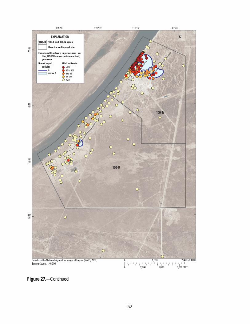
52
Figure 27.—Continued

53
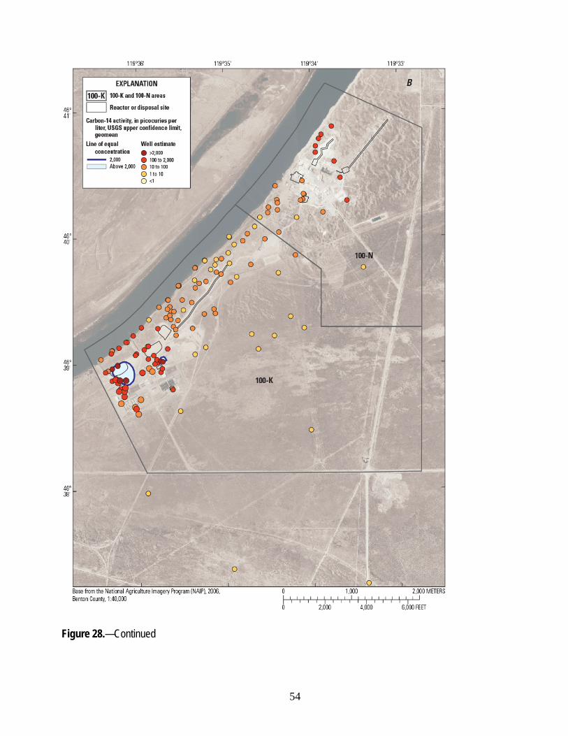
Figure 28. Maps showing carbon-14 plumes for (A) average (geomean) well values, (B) upper (95 percent) confidence limits on well averages, and (C) lower (5 percent) confidence limits on well averages, Hanford Site, Washington.
54
Figure 28.—Continued

55
Figure 28.—Continued

56
The areas of plumes as delineated by the USGS and DOE are given in table 1. The estimates agree to within about 40 percent, except for hexavalent chromium for which the USGS calculates an area that is more than twice the estimate by the DOE. The estimates also give a fairly consistent ranking to the relative sizes of the plumes: two or three large (about 0.5 km2 or larger) plumes are present for strontium-90, nitrate, and possibly hexavalent chromium (the last is intermediate according to DOE calculations); tritium is intermediate in size (about 0.2 km2); and the carbon-14 plume area is smallest at about 0.08 km2. Hexavalent chromium, tritium, and carbon-14 are primarily (or entirely) in the 100-K Area, whereas strontium-90 is primarily in the 100-N Area. Nitrate is about evenly distributed between the 100-K and 100–N Areas, by the USGS calculation, whereas the DOE plume for nitrate occurs more in the 100-N Area.
The volumes of contaminated groundwater are shown in table 2. Note that the DOE calculations are not actually from a DOE source, but use only the DOE plume extents, and are calculated using USGS aquifer saturated thicknesses. As a result, the comparisons among the contaminants are similar to differences among the delineated plume areas. The locations of the plumes are similar in both plume delineations and so the aquifer saturated thickness is close in the two estimations. The average saturated thickness of contaminated aquifer (volume divided by area, adjusting out the porosity) is about 19 m for both delineations and contaminants, though only about 11 m saturated thickness for strontium-90 because it is detected in an area with a thin aquifer, and about 23 or 26 m saturated thickness for tritium and carbon-14.
The following subsections discuss each of the contaminants and the plumes delineated by the DOE and the USGS. The DOE plumes are shown in figures 7–11 and the USGS plumes in figures 17–21.
Hexavalent Chromium Both the DOE and USGS show plume extents for hexavalent chromium (figs. 7 and 17) with
high levels in four areas of the study area, almost all within the 100-K Area, running into the river, and spaced about evenly along the river. The most northeasterly of the DOE plume areas, the one that runs along the boundary between the 100-K Area and the 100-N Area, is shown as a single plume by the DOE but the USGS shows three separate areas. There also is another small area delineated by the USGS farther northeast, inside the 100-N Area, around a single well (199-N-80, fig. 17) that is not shown on the DOE plume, although there is a different (also isolated) well (199-N-18, fig. 7) nearby with measured values greater than the MCL.
In other areas, the plumes are broken up differently into sub-areas between the two analyses. An effect of the minimum curvature spatial interpolation, which the USGS used, can be seen in the plumes (fig. 17) farthest southwest, where the plume extents bleed off to the west because of a lack of other points (wells) in that direction that could have helped avoid extrapolation of higher concentrations.
Tritium The overall appearances of the tritium plumes as delineated by DOE (fig. 8) and by USGS (fig.
18) are very similar. There are some details that illustrate differences in spatial interpolation. The DOE shows one plume area in the northeastern (100-N) area, where the USGS shows four small areas greater than the MCL. In the southwestern (100-K) area, the DOE has three areas of plume whereas the USGS combines two of these into a single larger plume.

57
Nitrate Comparison of figures 9 (DOE plumes) and 19 (USGS plumes) for nitrate show a similar overall
pattern but some differences in details, apparently due to the interpolation methodology. In the southwestern part of the study area (the 100-K Area) the DOE mapping shows four separate plume pieces, whereas the USGS interpretation combines three of these into a larger plume, and two other areas with exceedances in isolated wells become very small plume areas, apparently broken up because of the presence of lower concentrations in nearby wells. In the northeastern part (the 100-N Area) the USGS analysis (fig. 19) has 10 separate plume areas that are combined into a single large area in the DOE interpretation (fig. 9).
Strontium-90 The strontium-90 plume delineations (figs. 10 and 20) appear very similar: a large plume in the
northeastern (100-N) area and several isolated small plumes in the southwestern (100-K) area. The USGS delineations (fig. 20) show five small areas in 100-K whereas the DOE delineation (fig. 10) has only four small areas of plume in 100-K.
Unlike other plumes, the large strontium-90 plume area in the 100-N Area has holes (one near well 199-N-32 in the DOE plumes [fig. 10], two in the USGS ones [fig. 20] with the second near well 199-N-80). These holes had to have special consideration when calculating areas and volumes. There also is a small area in the USGS plume delineation in the 100-N Area that is separate from and just to the west of the large plume (centered around the aquifer tubes C7934, C7935, and C7936, fig. 20) that does not appear to be included in the DOE plume delineation (fig. 10).
Carbon-14 The plume delineations by the DOE (fig. 11) and USGS (fig. 21) generally agree. There are only
two relatively small plume areas in the southwestern (100-K) area of the study area, one near the wells 199-K-34 and 199-K-106A, and the other near wells 199-K-29 and 199-K-30 (figs. 11 and 21). The main difference between these delineations is the area that is included near these wells.
Total Quantity of Contaminated Groundwater Similar to the areas, the estimates of volumes from the two analyses (table 2) are in good general
agreement, although it is the volumes of hexavalent chromium that have the greatest difference (the USGS estimate is more than twice the DOE estimate). The other estimates are within about 30 percent of each other. Most of this discrepancy is due to the differences in area, because both estimates are based on the same saturated aquifer thickness estimate.
Upper and Lower Limits The estimated upper limit and lower limit plumes (interpolating 95 percent or 5 percent
confidence levels for the mean) are shown in figures 24–28. In each figure, the part A shows the actual concentrations (average), the part B shows the upper limit, and part C shows the lower limit. In some cases, portions of the plumes are not visible in the lower limit interpretation or new pieces of plume appear in the upper limit version.

58
In addition, table 3 shows the relative differences (percentage change in total volume of contaminated groundwater) among these plume estimates. All plumes increase more in relative volume (about 45 percent increase), with the increase in contaminant concentration, than they decrease (about 27 percent decrease) with lowered concentration. The plume areas changed in a similar degree (51 percent increase and 27 percent decrease).
The method used for estimating these upper and lower limits on the plumes highly overestimates the uncertainly, because it assumes that the concentrations in all wells are simultaneously high (or low) at the same time. A better (but not feasible) methodology would involve a Monte Carlo type of simulation, where each of the well averages would be varied at random according to its own variance, and an estimate made of where 90 percent of the plumes of the estimated plumes would occur in this simulation.
Table 3. Differences in contaminant plume volume for extreme extents compared to average plume extents, Hanford Site, Washington.
Contaminant Upper limit difference (percent)
Lower limit difference (percent)
Hexavalent chromium + 64 - 37 Tritium
+ 56 - 44
Nitrate + 44 - 29 Strontium-90
+ 46 - 11 Carbon-14
+ 13 - 12
Error Analysis The plume extents that are developed in the previous section are the average (geometric mean)
value of the concentration (or activity) of the contaminant in a well during a representative period. The uncertainty in the estimates can be considered in terms of the processes (models) that are used. Errors enter into the procedure at each step in the modeling process. The modeling steps to obtain the plume extents can be explained as follows:
• Sampling and analysis—conversion of in situ geochemical conditions into an analytical value, problems that may arise from either an unrepresentative sample or a failure in the chemical analysis procedure.
• Environmental fluctuation—changes over time even in the same screen and well, and variations with depth between shallower and deeper wells
• Data selection—determining the most representative analytical values for the plume, including use of older wells where more recent data are not available
• Averaging—analytical values from multiple samples into a (log) mean value for a well or collocated well group
• Linearization—Conversion of well mean values into a (log-) normal distribution of values from across the study area and including treatment of below detection limit values
• Spatial interpolation—of the log-normal values across the study area, including interpolation methodology and density of grid points

59
• Delineation of lines of equal concentration—Delineation of the lines (plume extents), closure of these lines into polygons, and estimation of areas Further analysis to calculate the volumes of contaminated groundwater include several
additional model steps: • Data selection for further interpretation of data that can best describe the contaminated
aquifer and the plumes within it. o Top—water table altitudes o Bottom—top of RUM unit o Vertical variations (stratification) o Porosity
• Spatial interpolations of saturated aquifer thickness • Integration of aquifer volume Each of these modelling steps introduces errors in its processing of the data and the errors are
compounded in subsequent steps. Some of these errors can be detected in the data but most are simply components of the overall variation in the data. Because they are combined in the data, it is difficult to differentiate sources or quantify the errors from the various factors.
An estimate for the total variation in the analytical results and environmental fluctuation is the distribution of (log) values reported for each well, around the mean (log) value at that well location. It was determined that the median residual (in the log values) was approximately 14 percent, or (converting from the log transform) a factor of 1.37 on either side of the mean. The calculation could not include non-detects or wells with only one measurement, so the errors in the distributions may be greater than this estimate. However, this variability appears small compared to the range of values plotted in the plumes.
This variability includes those of a temporal or environmental nature, at least over the time period (approximate 3-year) selected for most of the data. This was investigated over some datasets of concentrations over larger time periods. For example, it was determined that changes in concentration for wells near the Columbia River were associated with water level fluctuations in the river, probably by moving higher groundwater concentrations into or out of screened zones in the wells. Because of the limited data, and the presence of other factors, these changes could not be adjusted in the present analysis.
One component that may be observed in some isolation is analytical error, because the data files include the laboratory estimate of total propagated analytical uncertainty based on a 2-sigma error. A more extensive selection of analytical data for each of the analyzed contaminants of interest was extracted from the online files of historical data (Rieger, 2012), for the entire Hanford Site rather than just in the study area, including all detected values that passed quality control review and had this parameter reported. This analytical uncertainty parameter was normalized by dividing by the reported concentration for the sample, to get a relative error for the sample and contaminant. The median relative total analytical error for these analyses was approximately 17 percent of the sample result for the five contaminants of concern. Because these analytical errors are reported to be a 2-sigma error (that is, bracketing 95 percent of the variation), the median error (bracketing 50 percent of the variation) from analytical causes would be smaller.

60
The error in fitting the plumes after the interpolation is best estimated by the residual between the well mean value and the interpolated value at that well location. This metric was investigated briefly and it was determined that much of the difference (error), when using the minimum curvature method on this dataset appears to come from multiple well locations that may be found within a 50 × 50-m cell. Even at the much finer scale of the fine (10-m) grid cells there were still multiple wells overlapping in cells. Removing the collocated wells in the data selection process (considered the same location if within a radius of 2 m) did not eliminate all the well clusters.
A potentially major source of error is the interpolation methodology used. As shown in figure 16, the outlines of the plumes can be very different when different methodologies are used; also shown is the effect of using a fine grid (the 10-m grid used for the contaminated volume calculation) even with the same minimum curvature methodology and the same well and concentration dataset. In addition, there are many variables that may be adjusted within each of these methodologies and different plume configurations would result. It can be seen that variations in interpolation methodology can change plume shapes and sizes considerably, but sensitivity analyses to show this were not possible for this study.
Limitations The interpolation methodology is based strictly on statistical and geostatistical (spatial
distribution) analysis of the data as available. Many factors were not considered in this analysis, such as: • hydrogeology, such as plume transport (especially effects of remediation projects either in
removing contamination or in affecting its distribution), variations in depth, or seasonal fluctuations;
• changes in concentration at wells not currently sampled but included from older sampling rounds to fill in gaps; and
• errors in sampling or analytical processing. These considerations were too complex to take into account in this study. The DOE plumes
incorporated some hydrogeology considerations and limited the time frame of the sampling to minimize changes in concentration. This may be a reason for some of the differences in results.
Summary The plumes that U.S. Geological Survey developed for groundwater concentration for five
contaminants of concern (hexavalent chromium, tritium, nitrate, strontium-90, and carbon-14) are similar in many regards with those previously published by the U.S. Department of Energy and its contractors. Neither methodology used for the two interpretations of plumes result in consistently larger or smaller extents, and the shapes of the plumes are similar in both analyses. Several alternative methodologies also were tested during the course of this investigation, but the differences in results were not different enough to justify inclusion here.
The data are too sparse and the geohydrologic influences are too complex to develop more precise plume delineations based on geospatial considerations within the scope of the project presented here. The U.S. Department of Energy has followed best practices in its interpretations, and has already used some of the methodologic enhancements which the U.S. Geological Survey would also utilize.
Finally, any reasonable objectives for data quality that may be required for the purposes of the injury assessment plan, which will be developed for the Hanford Natural Resource Trustee Council as part of the Natural Resource Damage Assessment, should be more than adequately satisfied by the data and interpretation that is supplied by the U.S. Department of Energy and its contractors.
61
References Cited Alexander, D.J., and Hartman, M.J., 2012, Section 2.4—100-NR-2, in U.S. Department of Energy,
Hanford site groundwater monitoring for 2011: U.S. Department of Energy, Richland Operations Office, DOE/RL-2011-118 (Revision 0), p. 2.4-1–2.4-34, accessed September 27, 2012, at http://www.hanford.gov/c.cfm/sgrp/GWRep11/start.htm.
Caron, F., Sutton, J., Benza, M.L., and Haas, M.K., 2000, Determination of carbon-14 levels in heavy water and groundwaters: Analyst, v. 125, p. 59–64, DOI: 10.1039/A906365J, accessed November 2014, at http://pubs.rsc.org/en/Content/ArticleLanding/2000/AN/a906365j#!divAbstract.
CH2M Hill, 2012a, Environmental dashboard application: CH2M Hill Plateau Remediation Company Prepared for the U.S. Department of Energy, accessed May 4, 2012, at http://environet.hanford.gov/eda/.
CH2M Hill, 2012b, Hanford site environmental data request, April 2012: CH2M Hill Plateau Remediation Company, presented to Hanford Site Natural Resource Trustee Council, prepared for the U.S. Department of Energy, received May 4, 2012.
Esri, 2014, ArcGISTM version 10.2.2 for desktop: Redlands, Calif., Environmental Systems Research Institute, http://www.esri.com.
Foss, D.L., and Charboneau, B.L., 2011, Groundwater remediation of hexavalent chromium along the Columbia River at the Hanford site in Washington state, USA, in ASME 2011 14th International Conference on Environmental Remediation and Radioactive Waste Management, Reims, France, September 25–29, 2011: American Society of Mechanical Engineers, doi:10.1115/ICEM2011-59030, http://proceedings.asmedigitalcollection.asme.org/proceeding.aspx?articleid=1645949.
Golden Software, Inc., 2015., Surfer version 13.0.383—Surfer® 13 full user’s guide: Golden, Colorado, Golden Software, Inc., 1,137 p. [Also available at http://www.goldensoftware.com.]
Hartman, M.J., 2012, Section 2.1—Introduction to the river corridor, in U.S. Department of Energy, Hanford site groundwater monitoring for 2011: U.S. Department of Energy, Richland Operations Office, DOE/RL-2011-118 (Revision 0), p. 2.1-1–2.1-18, accessed September 27, 2012, at http://www.hanford.gov/c.cfm/sgrp/GWRep11/start.htm.
Hanford Natural Resource Trustees, 2013, Hanford natural resource damage assessment—Injury assessment plan: Hanford Natural Resource Trustees, 427 p., accessed July 2, 2013, at http://www.hanfordnrda.org/wp-content/uploads/2011/12/Final_Hanford-Natural-Resource-Damage-Assessment-Injury-Assessment-Plan-with-Appendices.pdf.
Helsel, D.R., and Hirsch, R.M., 2002, Statistical methods in water resources: U.S. Geological Survey, Techniques of Water Resources Investigations, book 4, chap. A3, 522 p., http://pubs.usgs.gov/twri/twri4a3/.
Hoitink, D.J., Burk, K.W., Ramsdell, J.V., Jr., and Shaw, W.J., 2005, Hanford site climatological summary 2004 with historical data: Richland, Washington, Pacific Northwest National Laboratory, PNNL-15160, 192 p., http://www.pnl.gov/main/publications/external/technical_reports/PNNL-15160.pdf.
Ivarson, K.A., Miller, C.W., and Hartman, M.J., 2012, 100-KR-4, in U.S. Department of Energy, Hanford site groundwater monitoring for 2011: U.S. Department of Energy, Richland Operations Office, DOE/RL-2011-118 (Revision 0), p. 2.3-1–2.3-34, accessed September 27, 2012, at http://www.hanford.gov/c.cfm/sgrp/GWRep11/start.htm.
Lichtenstein, N.D., 2004, The Hanford Nuclear Waste Site—A legacy of risk, cost and inefficiency: University of New Mexico School of Law, Natural Resources Journal, v. 44, no.3, p. 809–839, accessed February 2015, at http://lawschool.unm.edu/nrj/volumes/44/3/07_lichtenstein_hanford.pdf.
62
Martin, C.J., 2012, Appendix E—Overview of Hanford hydrogeology and geochemistry, in U.S. Department of Energy, Hanford site groundwater monitoring for 2011: U.S. Department of Energy, Richland Operations Office, DOE/RL-2011-118 (Revision 0), p. E-1–E-42, accessed September 27, 2012, at http://www.hanford.gov/c.cfm/sgrp/GWRep11/start.htm.
Oze, Christopher, Bird, D.K., and Fendorf, S., 2007, Genesis of hexavalent chromium from natural sources in soil and groundwater: Proceedings of the National Academy of Sciences of the United States of America, v. 104, no. 16., p. 6,544–6,549, accessed February 2015, at http://www.pnas.org/content/104/16/6544.full, DOI: 10.1073/pnas.0701085104.
Rieger, J.T., 2012, Data files—Electronic data for calendar year 2011, in U.S. Department of Energy, Hanford site groundwater monitoring for 2011: U.S. Department of Energy, Richland Operations Office, DOE/RL-2011-118 (Revision 0), p. E-1–E-42, accessed September 27, 2012, at http://www.hanford.gov/c.cfm/sgrp/GWRep11/html/data2011.zip.
Serne, R.J., 2007, Kd values for agricultural and surface soils for use in Hanford site farm, residential, and river shoreline scenarios: Richland, Washington, Pacific Northwest National Laboratory, PNNL-16531, 87 p.
Serne, R.J., and LeGore, V.L., 1996, Strontium-90 adsorption-desorption properties and sediment characterization at the 100 N-Area: Richland, Washington, Pacific Northwest National Laboratory, PNNL-10899/UC-702, 82 p., accessed March 24, 2016, at http://www.osti.gov/scitech/servlets/purl/186728.
Singleton, M.J., Woods, K.N., Conrad, M.E., Depaolo, D.J., and Dresel, P.E, 2005, Tracking sources of unsaturated zone and groundwater nitrate contamination using nitrogen and oxygen stable isotopes at the Hanford site, Washington: American Chemical Society, Environmental Science and Technology, v. 39, p. 3,563–3,570, http://pubs.acs.org/doi/abs/10.1021/es0481070.
U.S. Department of Agriculture, 2006, NAIP Imagery for Benton County, Washington: U.S. Department of Agriculture database, accessed January 29, 2008, at
https://gdg.sc.egov.usda.gov/GDGOrder.aspx. U.S. Department of Energy, 1992, Hanford site groundwater background: DOE/RL-92-23, accessed
March 23, 2016, at http://pdw.hanford.gov/arpir/pdf.cfm?accession=D196102655, 186 p. plus appendices.
U.S. Department of Energy, 2012a, Hanford site groundwater monitoring for 2011: U.S. Department of Energy, Richland Operations Office, DOE/RL-2011-118 (Revision 0), accessed September 27, 2012, at http://www.hanford.gov/c.cfm/sgrp/GWRep11/start.htm.
U.S, Department of Energy, 2012b, Waste inventories for cumulative impact analyses: U.S. Department of Energy, Richland Operations Office, Final Tank Closure and Waste Management Environmental Impact Statement, DOE/EIS-0391, DOE/EIS-0391 and Supporting Documents Web page, http://www.hanford.gov/page.cfm/FinalTCWMEIS.
U.S. Department of Energy, 2016, Hanford history: U.S. Department of Energy, Hanford Site Web page, accessed August 26, 2016, at http://www.hanford.gov/page.cfm/HanfordHistory.
U.S. Environmental Protection Agency, 2000, Air toxics web site—Chromium compounds: U.S. Environmental Protection Agency Web page, accessed February 2015, at https://www3.epa.gov/airtoxics/hlthef/chromium.html.
U.S. Environmental Protection Agency, 2002, EPA facts about strontium-90: Washington, D.C., Environmental Protection Agency, 2 p., accessed February 18, 2015, at http://www.epa.gov/superfund/health/contaminants/radiation/pdfs/strontium.pdf.

63
U.S. Environmental Protection Agency, 2014, EPA Facts about tritium: Washington, D.C., Environmental Protection Agency, 2 p., accessed February 18, 2015, at http://www.epa.gov/superfund/health/contaminants/radiation/pdfs/Tritium%20Fact%20Sheet%20final.pdf.
U.S. Geological Survey, 2000, National Elevation Dataset: 30m resolution, UTM zone 10, NAD83, accessed August 7, 2012, at: https://catalog.data.gov/dataset/usgs-national-elevation-dataset-ned.
U.S. Geological Survey, 2012, USGS 12472800 Columbia River below Priest Rapids Dam, WA:, U.S. Geological Survey National Water Information System, accessed September 7, 2012, at http://waterdata.usgs.gov/wa/nwis/dv/?site_no=12472800.
Waichler, S.R., Perkins, W.A., and Richmond, M.C., 2005, Hydrodynamic simulation of the Columbia River, Hanford reach, 1940–2004: Pacific Northwest National Laboratory, Prepared for the U.S. Department of Energy under Contract DE-AC05-76RL01830, PNNL-15226, 193 p., accessed January 28, 2015, at http://www.pnl.gov/main/publications/external/technical_reports/PNNL-15226.pdf
64
Appendix A. Calculation Spreadsheets for Groundwater Contaminant Plume Maps and Volumes, 100-K and 100-N Areas, Hanford Site, Washington
Appendix A is a Microsoft Excel® file that is available for download at http://dx.doi.org/10.3133/ofr20161161.

Publishing support provided by the U.S. Geological SurveyScience Publishing Network, Tacoma Publishing Service Center
For more information concerning the research in this report, contact the Director, Washington Water Science Center
U.S. Geological Survey 934 Broadway, Suite 300 Tacoma, Washington 98402 http://wa.water.usgs.gov

Johnson—G
roundwater Contam
inant Plume M
aps and Volumes, 100-K and 100-N
Areas, H
anford Site, Washington—
Open-File Report 2016-1161
ISSN 2331-1258 (online)http://dx.doi.org/10.3133/ofr20161161