Continental Shelf Research 20 (2000) 2067–2093

The structure of the Eel River plumeduring floods

W. Rockwell Geyera,*, P. Hillb, T. Milliganc, P. Traykovskia

aApplied Ocean Physics and Engineering Department, Woods Hole Oceanographic Institute,

Woods Hole, MA, USAbDepartment of Oceanography, Dalhousie University, Halifax, Nova Scotia, Canada

cHabitat Ecology Section, Bedford Institute of Oceanography, Dartmouth, Nova Scotia, Canada

Abstract

Several large floods of the Eel River in northern California occurred during 1997 and 1998,

with peak discharge ranging from 4000 to 12,000 m3 sÿ 1. The flood conditions persisted for1–3 days and were usually accompanied by strong winds from the southern quadrant. Thestructure of the river plume was strongly influenced by the wind-forcing conditions. During

periods of strong southerly (downwelling favorable) winds, the plume was confined inside the50-m isobath, within about 7 km of shore, with northward velocities of 0.5–1m sÿ 1.Occasional northerly (upwelling favorable) winds arrested the northward motion of the plume

and caused it to spread across the shelf. Sediment transport by the plume was confined to theinner shelf (water depths less than 50m), during both southerly and northerly wind conditions.During southerly wind periods, fine, unaggregated sediment was rapidly transportednorthward to at least 30 km from the river mouth, but flocculated sediment was deposited

within 1–10 km of the river mouth. During northerly (upwelling-favorable) winds, most of thesediment fell out within 5 km of the mouth, and negligible sediment was carried offshore, eventhough the low-salinity plume extended beyond the 60-m isobath. Although sediment

deposition from the plume is confined to the inner shelf, the stratigraphy indicates that theprincipal flood deposits on the adjacent continental shelf occur in a patch between the 60- and90-m isobath. Thus, the deposition on the inner shelf is ephemeral, and some mechanism other

than plume transport delivers the sediment from the inner shelf to the mid-shelf. # 2000Elsevier Science Ltd. All rights reserved.

Keywords: River plumes; Sediment transport; Eel River; Floods

*Corresponding author.

0278-4343/00/$ - see front matter # 2000 Elsevier Science Ltd. All rights reserved.

PII: S 0 2 7 8 - 4 3 4 3 ( 0 0 ) 0 0 0 6 3 - 7

1. Introduction

Milliman and Syvitski (1992) determined that a large fraction of the sedimententering the oceans from continents comes from small, high-relief drainage basins.The delivery of sediment from these rivers to the coastal ocean occurs in freshwaterplumes, whose trajectories may strongly influence the ultimate fate of the sediment(Morehead and Syvitski, 1999). The dynamics and structure of plumes of small riversdiffer considerably from those of large rivers, due to differences in the physical scalesof the processes near the river mouth (Garvine, 1995) and relatively short duration offloods from small, high relief rivers compared to large river systems (Nash, 1994).

The short duration of flood events in small rivers may lead to a more importantrole of synoptic scale (1–5 day duration) meteorological forcing on the trajectory ofthe plume than in large river systems. Large rivers such as the Amazon or theMississippi have freshet periods that extend over months, so the fate of the dischargeplume depends on forcing conditions over seasonal time scales (Lentz andLimeburner, 1995; Geyer et al., 1996). Small and intermediate-size rivers with steepdrainage basins exhibit markedly different behavior; freshet events can be extremelyshort-lived, occurring virtually on the same time scale as the meteorological eventsthat supply the precipitation. Thus, the wind forcing during the brief period of highflow may determine the structure of the plume (Chao, 1988b) and the fate of thesediment discharged onto the continental shelf.

The transport of sediment in river plumes is controlled not only by the trajectoryof the freshwater plume, but also by settling. Over the shallow, inner continentalshelf, river plumes may remain in contact with the bottom boundary layer,whereas in deeper water, the plume separates from the bottom (Yankovsky andChapman, 1997). After the plume has separated from the bottom boundary layer,sediment can no longer be maintained in the water column via resuspension, so ariver plume will start to lose sediment as soon as it separates from the bottomboundary layer. The trajectory of sediment within the plume thus depends on therate of settling, the plume thickness and plume velocity. The freshwater plume maybe much more extensive than the sediment plume, particularly if the velocities in theplume are low, allowing the sediment to settle out before being carried far from themouth.

A recent study of the Eel River in northern California provides an unprecedentedset of observations of the structure of a plume emanating from a small, high-reliefriver during floods. The Eel River has one of the highest rates of sediment supplyrelative to area of any North American river (Brown and Ritter, 1971). The sedimentload is dominated by brief, severe floods that occur during the winter months.During one flood in January, 1995, the Eel delivered an estimated 22 million tons ofsediment to the coastal ocean (Wheatcroft et al., 1997). A distinct flood deposit offine-grained sediment with a thickness of up to 10 cm and a length of 30 km wasidentified from sediment cores on the Eel River shelf between the 60- and 90-misobaths. One possible explanation for the distribution of sediment on the shelf is thetrajectory of the freshwater plume. However, lack of information about the shapeand velocity of the Eel River plume and of settling velocity of sediment within it

W.R. Geyer et al. / Continental Shelf Research 20 (2000) 2067–20932068

made it difficult of assess whether the plume could have delivered the sedimentdirectly to the flood deposit.

A field study was undertaken in the winters of 1996–1997 and 1997–1998 todetermine the structure of the Eel River plume during floods, to quantify thetransport of suspended sediment by the plume, and to assess its role in the formationof flood deposits. A large flood event occurred in January 1997, comparable inmagnitude to the 1995 event. Several moderate events also occurred in the winter of1998, due to the high rainfall associated with El Nino conditions. A combination ofhelicopter surveys and moorings provided measurements of salinity, temperature,suspended sediments and currents within the plume and the adjacent waters overthe continental shelf. These observations provide the basis for an analysis of thedynamics of the plume and its freshwater and sediment transport during floods. Thesediment transport calculations are then used to determine the role of the plume inthe delivery of sediment to the continental margin and in the formation ofsedimentary deposits on the continental shelf.

2. Methods

2.1. Site description

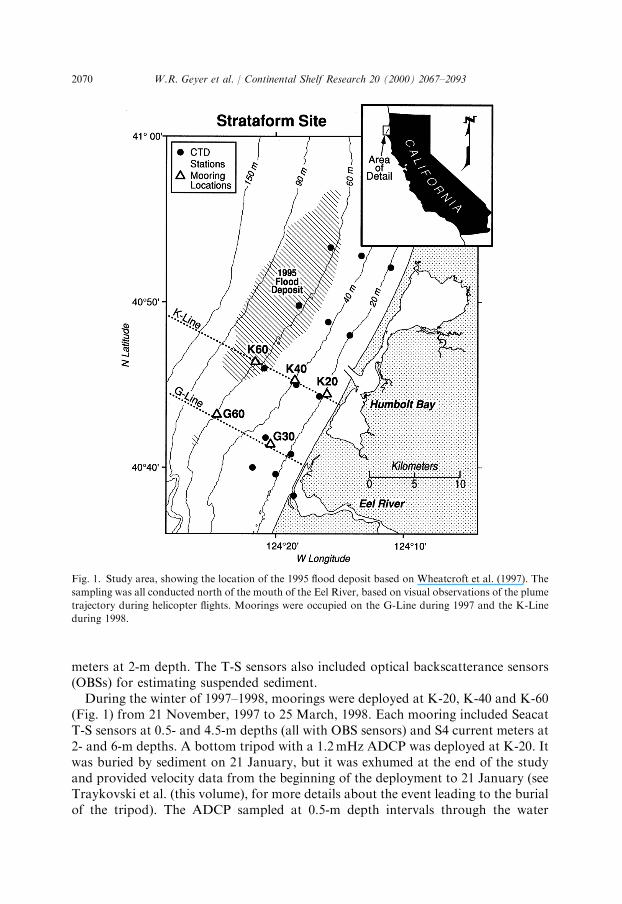
The Eel River enters the Pacific Ocean just north of Cape Mendicino, in NorthernCalifornia (Fig. 1). Its discharge is generally low, but it usually has one or more largeflows, lasting for several days, during the passage of winter storms (Brown andRitter, 1971; Syvitski and Morehead, 1999). The Eel River has an unusually highsediment yield relative to its drainage area, due to the high relief and easily erodedbedrock (Brown and Ritter, 1971). The continental shelf adjacent to the river mouthis 10–15-km wide. During the winter months, the water column is weakly stratified,except during periods of high river flow (Largier et al., 1993).

The surficial sediment distribution on the shelf is dominated by sand at depths lessthan 50-m and by fine silt at greater depths (Borgeld et al., 1999). 210Pb inventoriesindicate a depositional zone to the north of the mouth of the Eel, corresponding inlocation to the 1995 flood deposit, with accumulation rates as high as0.8 g cmÿ 2 yrÿ 1 (Sommerfield & Nittrouer, 1999). Fine sediment accumulation alsooccurs on the continental slope at distances >50 km north of the mouth of the Eel,at rates of 0.2–0.4 g cmyrÿ 1 (Alexander and Simoneau, 1999).

2.2. Moored measurements

Moorings and tripods were deployed on the Eel Shelf in the winters of 1996–1997and 1997–1998. In 1996–1997, moorings were also deployed at the 30- and 60-misobath along the G-line (G-30 and G-60; see Fig. 1), for the period 16 December1996–February 23 1997. The moorings consisted of surface buoys with Seacattemperature–salinity (T-S) sensors mounted to them at 0.5-m depth and S4 current

W.R. Geyer et al. / Continental Shelf Research 20 (2000) 2067–2093 2069

meters at 2-m depth. The T-S sensors also included optical backscatterance sensors(OBSs) for estimating suspended sediment.

During the winter of 1997–1998, moorings were deployed at K-20, K-40 and K-60(Fig. 1) from 21 November, 1997 to 25 March, 1998. Each mooring included SeacatT-S sensors at 0.5- and 4.5-m depths (all with OBS sensors) and S4 current meters at2- and 6-m depths. A bottom tripod with a 1.2mHz ADCP was deployed at K-20. Itwas buried by sediment on 21 January, but it was exhumed at the end of the studyand provided velocity data from the beginning of the deployment to 21 January (seeTraykovski et al. (this volume), for more details about the event leading to the burialof the tripod). The ADCP sampled at 0.5-m depth intervals through the water

Fig. 1. Study area, showing the location of the 1995 flood deposit based on Wheatcroft et al. (1997). The

sampling was all conducted north of the mouth of the Eel River, based on visual observations of the plume

trajectory during helicopter flights. Moorings were occupied on the G-Line during 1997 and the K-Line

during 1998.

W.R. Geyer et al. / Continental Shelf Research 20 (2000) 2067–20932070

column. Sampling periods of the instruments varied from 5 to 30min. All of the datawere averaged to 1 h.

2.3. Helicopter surveys

‘‘Rapid Response’’ helicopter surveys were conducted with the assistance of theCoast Guard Group Humboldt Bay during major river discharge events. Helicopterswere used rather than a research vessel because of the typically extreme seaconditions during floods. An instrument package was deployed using the helicopter’swinch to obtain vertical profiles of water properties and to obtain discrete watersamples. The package included an Ocean Sensors CTD and OBS, two 1.5–l Niskinbottles, and a floc camera for imaging particles. The Niskin bottles wereautomatically triggered at 1.5- and 10-m depths. The flights lasted for 1.5–2 h, and3–14 stations were occupied, depending on weather conditions and otherresponsibilities of the flight crew. During the 1996–1997 observations, the instrumentpackage did not reach the bottom, but during the 1997–1998 observations, the sensorpackage was lowered to the bottom at most stations (Fig. 1).

The CTD sampled at 2Hz during the 1996–1997 observations and 5Hz in 1998,corresponding to vertical resolution of 0.3- and 0.1-m, respectively. The watersamples were transferred into 1-l Nalgene bottles onboard the helicopter and werefiltered for total suspended solids using an 8 mm fiberglass filter. Disaggregatedsediment size distributions were determined using a Coulter Counter (Milligan andKrank, 1991) and in situ floc size distributions were calculated by size analysis ofphotographs taken by the floc camera (Hill et al., this volume).

The OBS on the profiler was calibrated against the bottle data, aggregating all ofthe data from each year. There were no significant differences between the responsecurves for different cruises. For 1996–1997, the regression coefficient was r2 ¼ 0:95(n ¼ 31) for the calibration. For the 1997–1998 data, the calibration of theinstrument was adjusted after the seventh survey to extend the range of measure-ments, so there were separate calibrations for the two settings. The regressioncoefficient for the first calibration was r2 ¼ 0:81 (n ¼ 43) and the regression for thesecond set was r2 ¼ 0:96 (n ¼ 21). The calibration of the moored OBS sensors wasaccomplished based on point comparisons with bottle samples during the helicoptersurveys. The measurements were also compared to values from the surveys. Therewas evidence of fouling in both OBS records at K-60 and the deep sensor at K-40during 1998, based on rapidly increasing backscatter at the ends of the timeseriesthat was uncorrelated with other hydrographic properties. Fouling did not appear tobe a problem during the shorter deployment in 1996–1997, and there was noevidence of fouling of the instruments at K-20 or the surface instrument at K-40during 1997–1998.

A total of seven surveys were performed in 1996–1997, nine in 1997–1998, andfour in 1998–1999. This paper focusses on a major flood that occurred from 30December 1996 to 3 January 1997, and a series of floods in January and February,1998.

W.R. Geyer et al. / Continental Shelf Research 20 (2000) 2067–2093 2071

2.4. Other data

Wind and wave data were obtained from the NOAA buoy NDBC 46022, locatedat the 150-m isobath near the G-line, and NDBC 46030, located near CapeMendicino, approximately 30-km south of the mouth of the Eel. Buoy 46022 datawere used during 1997–1998, but the data were unavailable during early January,1997, so the 46030 data were used for the 1996–1997 analysis. River discharge datawere obtained by two USGS gauging stations: the Eel River at Scotia and the VanDuzen at Bridgeville, which together account for more than 90% of the flow of theEel at the mouth.

3. Results

3.1. New-Year’s flood, 1996–1997

The forcing conditions for the large 1997 event are shown in Fig. 2. This event hadthe highest discharge recorded since 1964 (Brown and Ritter, 1971), during which thelargest recorded flood occurred. The high flow occurred over a 3-day period duringwhich a major storm supplied high precipitation and strong southerly winds. Windspeaked at 20m sÿ 1 on 31 January, close to the time that the river flow first exceeded10,000m3 sÿ 1. The southerly winds subsided to 10m sÿ 1 for the next two daysduring the peak flow of the river, and on 3 January, the low-pressure system movedlandward and the winds abruptly shifted to northerly. The along-shelf currents at2-m depth at G-30 approximately tracked the winds, with the addition of a tidaloscillation of � 30 cm sÿ 1. The surface salinity at G-30 indicates that the freshwaterplume only briefly reached the mooring on 28 December, and it did not reappearuntil 3 January, following the wind reversal. Thus for most of the discharge event,the measured currents reflect conditions outside the river plume.

Analysis of the moored data for the whole deployment period at G-30 and G-60indicates that the along-shelf currents are highly correlated across the shelf (r ¼ 0:84between the surface currents at the two locations). The along-shelf currents are alsohighly correlated with the winds (At G-60, near- surface, r ¼ 0:70 at 9 h lag; at G-30,near-surface, r ¼ 0:65, 4 h lag). These statistics indicate that the shift in along-shelfcurrents following the wind reversal on 3 January is typical of the along-shelfresponse during the winter months. Likewise the strong along-shelf currents duringthe peak discharge can be attributed mainly to the wind forcing.

Although the G-30 mooring was too far offshore to provide information about theplume during the flood, there were four helicopter surveys during the event (notetimes indicated by the triangles in Fig. 2) that document the structure of the plume.The surface salinity distribution (Fig. 3) indicates that the plume was narrowerduring the downwelling period (31 December and 2 January), even though this wasthe time of maximum outflow. Only after the winds reversed on 3 January did theplume begin to spread offshore. The measurements on 2 January included data in thenearshore part of the plume (along the 20-m isobath); these indicated surface

W.R. Geyer et al. / Continental Shelf Research 20 (2000) 2067–20932072

salinities of 15–20 psu compared to an ambient shelf salinity greater than 32. Thevertical structure of the plume is indicated in cross-sections at the K-line (Fig. 3,lower panels). The plume was 6–7-m thick at the K-line during downwelling-favorable winds, and it thinned to 3m as it extended offshore during the afternoon of3 January, forced by upwelling-favorable winds.

The suspended sediment distribution (Fig. 4) closely resembled the salinitydistribution during the first two surveys (high flow and downwelling condition), withconcentrations of as much as 1500mg lÿ 1 within the plume, and negligible sedimentoutside the plume. During the last two surveys (falling flow, upwelling-favorablewinds), concentrations still reached 1000mg lÿ 1 at the G-line (3–5-km north of themouth), but the concentrations fell off sharply both in the offshore and along-shoredirections within the plume. The vertical structure of the sediment distribution wassimilar to salinity during the first two surveys, with a strong concentrationgradient at the base of the plume. In contrast, the concentration was relativelyuniform with depth on the third survey and increased with depth on the fourth

Fig. 2. Timeseries of forcing variables and conditions at the G-line during the large, 1997 flood. Top

panel: Eel River discharge (measured at Scotia); second panel: along-shelf wind measured at NOAA buoy

46030 (near Cape Mendicino); third panel: wave height measured at buoy 46030; fourth panel: along-shelf

velocity at G-30, 2m below the water surface; bottom panel: salinity at g-30, 0.5m below the water surface.

Times of helicopter surveys are shown by triangles.

W.R. Geyer et al. / Continental Shelf Research 20 (2000) 2067–2093 2073

survey. These observations indicate that the suspended sediment was behavingnearly conservatively within the plume during the high-flow, downwelling condi-tions, and that sediment was being lost to settling during the falling-flow, upwellingconditions.

A vertical section along the plume, following the 20-m isobath in the along-shelfdirection (Fig. 5) demonstrates that the plume was confined to the near-surfacewaters. Near the mouth, the plume was only 3-m thick, and it increased to 6–8-mthickness by 18-km north. The plume spread more in the vertical on January 2during southerly winds, suggesting mixing at the base of the plume, whereas the baseof the plume remained intact on January 3 during weak northerly winds, suggestingthe absense of mixing. Discrete suspended sediment measurements along this sectionindicate nearly conservative behavior of sediment within the plume on January 2,with high concentrations persisting to 18-km north. On January 3, the concentra-tions in the plume dropped by a factor of 4 at 11-km and by a factor of 50 at 18-km,indicating much more loss of sediment from the plume during the upwellingconditions. Concentrations beneath the plume increased between the mouth and11-km, consistent with the raining out of sediment from the plume.

Fig. 3. Salinity distributions from helicopter surveys during the January 1997 flood. Upper panels: near-

surface (1.5m) salinity distributions; lower panel: cross-sections at the K-line. The seaward limit of the

plume was estimated by visual observation from the helicopter.

W.R. Geyer et al. / Continental Shelf Research 20 (2000) 2067–20932074

3.2. 1998 floods

The discharge peaks of the 1998 floods were approximately one third theamplitude of the large 1997 flood, but the multiple events provides a variety offorcing conditions (Fig. 6). Three events that occurred under distinctly differentforcing conditions are shown by the dashed lines. The first (15 January 1998, labeled‘‘slow’’) corresponds to a peak discharge during a wind reversal (i.e., northerlywinds), the second (17 January, labeled ‘‘fast’’) to high flow with strong southerlywinds, and the third (19 January, labeled ‘‘rough’’) to moderate southerly winds butextreme wave conditions. Currents measured at the K-line during this period showthe wind-driven, along-shelf motions on which tidal currents are superimposed. Thealong-shelf currents were close to zero during the ‘‘slow’’ period; they were morethan 50 cm sÿ 1 along-coast during the ‘‘fast’’ period, and they were around40 cm sÿ 1 during the ‘‘rough’’ period. The salinity and turbidity do not consistentlytrack the inputs from the river (Fig. 6), due to variations in cross-shelf structure ofthe plume during different wind conditions. For example, large peaks in turbidity atK-20 occurred during several of the large discharge events, but they were absent

Fig. 4. Total suspended sediment distributions from helicopter surveys during the 1997 flood. Upper

panels: near-surface (1.5m) suspended solids, based on water samples; lower panel: cross-sections at the

K-line, based on water samples and OBS profiles.

W.R. Geyer et al. / Continental Shelf Research 20 (2000) 2067–2093 2075

during the events that occurred during upwelling-favorable winds (e.g., January 15and 26).

The variability of the plume structure as a function of forcing conditions isrevealed in cross-sections of salinity and suspended sediment (Fig. 7). The salinityplume extended farthest across the shelf during upwelling-favorable (or ‘‘slow’’)conditions, but the suspended sediment distribution was most limited during thesetimes. The suspended sediment and salinity had similar spatial structure duringdownwelling-favorable winds, i.e. ‘‘fast’’ conditions, and the high concentration ofsuspended sediment extended further offshore than during ‘‘slow’’ conditions. Thisdifference is explained by the shorter transit time within the more rapidly advectingplume, which provided less time for settling to occur. A notable feature of thesediment distribution in all cases was a bottom turbid layer; this layer was muchthicker and had much higher concentrations during the ‘‘rough’’ conditions. Theconcentration could not be resolved by the vertical profiles, because it exceeded thegain setting of the OBS (C>450mg lÿ 1).

There is evidence that the concentrations were much higher than 450mg/l in thisnear-bottom zone during the ‘‘rough’’ conditions. The apparent salinity measured bythe CTD dropped by as much as 1 psu near the bottom at K-20 (Fig. 8), which maybe explained by the reduced conductivity of high concentrations of suspended

Fig. 5. Along-shelf vertical sections at the 20-m isobath of salinity on January 2 1997 (near the peak of the

flood) and January 3 1997 (after the wind had shifted to northerly). Bold numbers are suspended sediment

measurements from water samples. (Note that some 10-m samples were not obtained during the January 2

survey).

W.R. Geyer et al. / Continental Shelf Research 20 (2000) 2067–20932076

sediment (Kineke and Sternberg, 1992). Calculations by Traykovski et al. (thisvolume) indicate that such a decrease in apparent salinity would requireconcentrations in the fluid mud range (50–100� 103mg lÿ 1). In addition, the outputof the OBS decreased abruptly within the turbid layer (Fig. 8). Kineke and Sternberg(1992) showed that at fluid mud concentrations, the output of the OBS actuallydecreases. For the gain setting of this instrument this effect would not be observeduntil the concentrations reached approximately 50� 103mg lÿ 1. Additional, perhapsmore direct, evidence comes from the moored ADCP data at this location.Approximately 5 h after the helicopter CTD observations of January 19, the ADCPwas buried under nearly 1-m of sediment (see Traykovski et al. (this volume) formore details).

Fig. 6. Timeseries of forcing variables and conditions at the K-line during a series of moderate discharge

events in 1998. Top panel: Eel River discharge; second panel: along-shelf wind measured at NOAA buoy

46022 (near the mouth of the Eel); third panel: wave height measured at buoy 46022; fourth panel: along-

shelf velocity at K-20 (solid) and K-40 (dashed), 2-m below the water surface; fifth panel: salinity at K-40,

0.5m below the water surface; bottom panel: suspended sediment at K-20 (solid) and K-40 (dashed), 0.5m

below the surface. (The salinity sensor at K-20 was clogged and did not provide useful data during this

period). The three time periods labeled ‘‘slow’’, ‘‘fast’’ and ‘‘rough’’ correspond to cross-sections in Fig. 7.

Times of helicopter surveys are shown by triangles.

W.R. Geyer et al. / Continental Shelf Research 20 (2000) 2067–2093 2077

The salinity and suspended sediment profiles can be compared to the velocitystructure at K-20 for the helicopter surveys prior to January 20, before the ADCPwas buried (Fig. 8). Both salinity and velocity showed strong vertical gradientsthrough the plume (down to 6–10-m depth), and they were uniform beneath theplume. There was no evidence of a surface mixed layer } the salinity gradientextended to within 1-m of the surface, even on January 14 when the wind velocitiesreached 10m sÿ 1. The suspended sediment profiles indicate approximately linear

Fig. 7. Cross-sections of suspended sediment and salinity structure of the plume at the K-line during three

time-intervals indicated on Fig. 6. The light shading correspond to low-salinity plume water with

suspended sediment concentrations C550mg l-1. The darker shading indicates higher suspended sediment

concentrations. Numbers indicate along-shelf velocities in cm s-1. The upper panel corresponds to ‘‘slow’’

conditions, when northerly winds slowed down the plume and caused offshore advection of fresh water.

The middle panel corresponds to ‘‘fast’’ conditions, when strong southerly winds caused rapid northward

advection. The bottom panel corresponds to ‘‘rough’’ conditions, when wave resuspension produced a

thick, high-concentration turbid layer with evidence of fluid mud. The plume structure landward of K-20 is

speculative; there were no observations in that region.

W.R. Geyer et al. / Continental Shelf Research 20 (2000) 2067–20932078

variation in concentration in the plume, except for January 15 in which the near-surface concentration decreased, most likely due to settling of sediment. A bottomturbid layer was evident in all of the profiles, with the highest near-bedconcentrations occuring on January 19. The downward spikes in the profile onJanuary 19 are evidence for extremely high concentrations, as noted above. Therewere large variations in barotropic (or vertically averaged) velocity, due both to tidesand wind-driven motions, but the shear was more closely tied to the salinity structure(see discussion).

4. Analysis and discussion

4.1. Dynamics of the plume and shelf region

4.1.1. TidesThe current meter observations indicate that the tides are mainly barotropic, with

semidiurnal velocity amplitudes of around 15 cm sÿ 1 and diurnal amplitudes around10 cm sÿ 1. The principal axes are oriented in the along-coast direction, and ellipticityis small near the coast but it increases offshore. When the semi-diurnal and diurnalcomponents were in phase, variations in along-shelf velocity of as much as 50 cm sÿ 1

occurred as a result of the tides, representing a significant perturbation on themotion of the plume. Tidal exchange through Humboldt Bay is also likely to affect

Fig. 8. Vertical profiles of salinity, velocity, and suspended sediment at K-20 during three helicopter

surveys in 1998. The velocity data were obtained from the bottom-mounted ADCP at the 20-m isobath,

whereas the salinity and suspended sediment data were obtained during helicopter surveys at the 26-m

isobath. The near-bottom sediment concentrations on January 19 are believed to be much higher than

indicated on the figure, as discussed in the text.

W.R. Geyer et al. / Continental Shelf Research 20 (2000) 2067–2093 2079

the plume, with an offshore-directed momentum source during ebb tides that iscomparable to the momentum of the river during peak discharge conditions (roughly10,000m3 sÿ 1 during large ebbs). The tidal jet should distort the plume and provideenergy for mixing and sediment resuspension. Some of the profiles indicatedsignificantly deeper penetration of brackish water to the north of the mouth ofHumboldt Bay relative to the profiles further south, suggesting that mixingassociated with the inlet may affect the plume. Because of this potential effect, theanalysis of plume transport processes was focussed to the south of the inlet.

4.1.2. Wind-driven motionsThe along-shelf winds provide a major source of variability of the along-shelf

currents. Based on linear regression between the moored velocity measurements atthe K-line and the NOAA Buoy 46022 winds in 1998, the near-surface, (2-m depth),along-shelf currents have a response of approximately 1m sÿ 1 per Pa of along-shelfwind stress. The strength of the response decreases to 20–40% of this value beneaththe plume. The currents lag the winds by roughly 6 h. Approximately 50% of thelow-frequency variance at the surface is explained by the wind stress, based onanalysis of the 1998 data at K-20 and K-40. There is also evidence of an Ekmanresponse of the cross-shelf currents to along-shelf wind stress, although it is only10% of the strength of the along-shelf response. The response to cross-shelf windswas not significant.

The nature and magnitude of the response to winds is consistent with othercontinental shelf observations and theory (Allen, 1980, Lentz and Winant, 1986,Lentz et al., 1999). Landward Ekman transport in the surface layer duringdownwelling-favorable winds causes a set-up of the sea surface against the coast anddeepening of the pycnocline, which drives a geostrophic flow that weakens withdepth due to the baroclinic gradient associated with the cross-shore salinity gradient.During upwelling winds, essentially the reverse process occurs, except that the cross-shelf baroclinic gradient is weakened as the plume advects offshore.

The winds are particularly important to the motion of the plume, because thealong-shelf winds are significantly correlated with river discharge, with northwarddirected wind stress tending to occur during high discharge conditions. Based on the1998 data, the peak wind stress leads the discharge by 1.5 days (correlationcoefficient r ¼ 0:46, degrees of freedom n > 20), but there is still significantcorrelation at 0 lag (r ¼ 0:24, n > 20). This correlation results from the associationof large precipitation events with low pressure systems, which produce strongsoutherly winds along the coast. In 1998, the average northward wind stress duringdischarge events (Q> 800 m3 sÿ1) was 0.15 Pa, which yields an average of 15 cm sÿ 1

of wind-induced, along-shelf flow at the surface, based on the above regressionanalysis. Non-event periods (Q5800 m3 sÿ1) had an average wind stress of 0.03 Pa,which is not significantly different from zero.

The wind stress strongly affects the cross-shelf structure of the river plume,consistent with previous studies (Chao, 1988b, Fong, 1998). Southerly (downwelling-favorable) winds confine the plume to the inner shelf, whereas the occasionalnortherly (upwelling-favorable) wind events spread the plume across the shelf. Wind

W.R. Geyer et al. / Continental Shelf Research 20 (2000) 2067–20932080

stress also appears to affect mixing within the plume, as inferred above in contextwith spreading at the base of the plume (Fig. 5). Note, however, that even with gale-force winds (e.g., Jan. 14, 1998; Fig. 6) the plume remained stratified to within 1-m ofthe water surface, indicating the strong stabilizing tendency of the buoyancy flux.Nor was there ever adequate stress for the resuspended sediment in the bottomboundary layer to affect the turbidity within the plume.

4.1.3. Riverine forcingThe freshwater inflow provides a direct input of momentum as well as a large

buoyancy source, both of which contribute to the motion over the shelf. Visualobservations from the helicopters as well as aerial photos indicate that over the last20 years, the Eel River has been deflected northward by a vegetated sand-spit, so thatit enters the ocean at an angle of about 208 to the along-shelf direction. Garvine(1982) showed that such an oblique angle of entry will produce a narrow, swift plumethat remains attached to the coast. The velocity at the mouth could not be estimatedprecisely, but it could be estimated from transport considerations. During the peakof the flood in 1997, the discharge was 12,000m3 sÿ 1, the width at the mouth wasapproximately 1-km (in the direction normal to the flow), and the depth wasestimated at 4–6m (based on one CTD cast taken in the river mouth on January 3,1997). This yields a peak outflow velocity of 2–3m sÿ 1. Some fraction of thismomentum input would have been lost to bottom friction within the surf zone andinner shelf, but even half of the initial velocity would still represent a majorcomponent of the momentum input for the plume.

The buoyancy forcing can be estimated from the baroclinic pressure anomalyassociated with the freshwater plume

Pf ¼ g

Z 0

ÿhðr0 ÿ rðzÞÞ dz; ð1Þ

where r0 is the ambient density, rðzÞ is the vertically varying density due to dilutionwith fresh water, and h is the water depth. The largest observed value of pf was360 Pa (on January 2, 1997 at G-20) which is equivalent to 3.7 cm of sea-leveldisplacement. Based on Bernoulli’s equation, it has the same dynamic pressure as avelocity anomaly of 85 cm sÿ 1. This indicates that the momentum flux from the riverexceeds the buoyancy forcing, or, equivalently, that the internal Froude number nearthe mouth exceeds 1 (Armi, 1986). The main implication of this supercritical flowcondition is that the dynamics in the vicinity of the mouth are strongly influenced bythe momentum input from the river (Garvine, 1995). The spatial scale of thisinfluence is defined by the inertial radius Li ¼ uf =f , where uf is a representativevelocity within the plume and f is the Coriolis acceleration. This scale was on theorder of 10-km during floods, indicating that inertial effects were importantapproximately as far as the K-line. The inertia of the outflow often produces a bulgein the plume adjacent to the mouth of a river with a scale close to the inertial radius(Chao and Boicourt, 1986); however the angle of the mouth of the Eel greatlyreduces the offshore extent of the bulge (Garvine, 1982). The bulge evident during

W.R. Geyer et al. / Continental Shelf Research 20 (2000) 2067–2093 2081

upwelling conditions (Fig. 3, third panel) was not due to inertia, but rather toconvergence of freshwater flux (see discussion below).

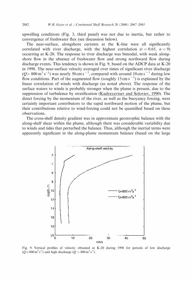
The near-surface, alongshore currents at the K-line were all significantlycorrelated with river discharge, with the highest correlation (r ¼ 0:65, n ¼ 9)occurring at K-20. The response to river discharge was bimodal, with weak along-shore flow in the absence of freshwater flow and strong northward flow duringdischarge events. This tendency is shown in Fig. 9, based on the ADCP data at K-20in 1998. The near-surface velocity averaged over times of significant river discharge(Q> 800 m3 sÿ1) was nearly 50 cm sÿ 1, compared with around 10 cm sÿ 1 during lowflow conditions. Part of the augmented flow (roughly 15 cm sÿ 1) is explained by thelinear correlation of winds with discharge (as noted above). The response of thesurface waters to winds is probably stronger when the plume is present, due to thesuppression of turbulence by stratification (Kudrayavtsev and Soloviev, 1990). Thedirect forcing by the momentum of the river, as well as the buoyancy forcing, werecertainly important contributors to the rapid northward motion of the plume, buttheir contributions relative to wind-forcing could not be quantified based on theseobservations.

The cross-shelf density gradient was in approximate geostrophic balance with thealong-shelf shear within the plume, although there was considerable variability dueto winds and tides that perturbed the balance. Thus, although the inertial terms wereapparently significant in the along-plume momentum balance (based on the large

Fig. 9. Vertical profiles of velocity obtained at K-20 during 1998 for periods of low discharge

(Q5800m3 s-1) and high discharge (Q > 800m3 s-1).

W.R. Geyer et al. / Continental Shelf Research 20 (2000) 2067–20932082

Froude number at the mouth), the relatively straight trajectory of the plumeproduced only a minor contribution of inertia to the cross-plume balance, leading toa semi-geostrophic regime typical of large river plumes (Garvine, 1995).

The observed freshwater transport within the plume is comparable to modelresults (Chao, 1988a) and observations (Rennie et al., 1999) of the plume fromChesapeake Bay, which has comparable transport to the Eel River plume duringfloods. The lowest mode internal wave speed within the plume was estimated at40–55 cm sÿ 1 based on the helicopter CTD profiles; thus the Froude number withinthe plume was close to 1 (in constrast to the Froude number at the mouth, whichsignificantly exceeded 1). The Froude number was significantly higher those found inthe model studies of Chao (1988a), in which the values ranged from 0.1 to 0.5. Thiscomparison indicates stronger forcing conditions for the Eel River plume, both dueto wind forcing and the momentum input at the mouth.

Several other plume parameters help characterize this plume for comparison withother regimes. The ‘‘mouth’’ Kelvin number (Garvine, 1987) is defined by Km ¼Lm=LD, where Lm ¼ 2 km is the width at the mouth and the deformation radius

LD ¼ ðg0hÞ1=2=f ¼ 5 km

(where g0¼ Dr=r is the buoyancy anomaly of the plume, h � 6m is the thickness ofthe plume, and f¼ 0:9� 10ÿ4 sÿ1 is the Coriolis parameter). Thus Km ¼ 0:4, whichindicates that inertial effects at the mouth are important relative to the earth’srotation (Garvine, 1987). The ‘‘plume’’ Kelvin number KP ¼ LP=LD, where LP is theplume width (Garvine, 1995) provides an indication of the overall importance ofrotation within the plume. The plume width LP � 6–8 km, indicating KP � 1. Thisputs the Eel River plume into the transition between advection-dominated androtation-dominated plumes.

Yankovsky and Chapman (1997) define a plume ‘‘lift-off ’’ depth hb ¼ð2Qp f =g

0Þ1=2 where QP is the total transport of brackish water in the plume. Atthe time of maximum river flow, the freshwater transport was about 104m3 sÿ 1, butmixing with salt water increased the total transport QP by a factor of 4–5. Theresulting lift-off depth hb � 13m for the maximum flow conditions. This calculationindicates, as is observed, that the plume should be detached from the bottom. Theobserved plume depth was roughly half of the calculated hb, which is probably due tothe along-shelf forcing of the plume by the plume by winds and barotropic currents,in contrast to the Yankovsky and Chapman theory in which baroclinic forcing is theonly ingredient.

4.2. Freshwater transport in the plume

The freshwater balance within the plume was used to estimate the residencetime of water within the plume and the advection speed of the plume. Thecalculation provides a characterization of the variability of the plume structureand provides important information for quantifying the sediment transport inthe plume. The input of freshwater into the plume Qf was based on the USGSgauging station data. The local ‘‘freshwater thickness’’ within the plume was

W.R. Geyer et al. / Continental Shelf Research 20 (2000) 2067–2093 2083

estimated by the integral

hf ¼1

s0

Z 0

ÿhðs0 ÿ sÞ dz ð2Þ

where s0 is the ambient salinity (taken as the maximum salinity in a particularsurvey), and s is the depth-varying salinity in the plume. This quantity can beregarded as the thickness of the plume if it were ‘‘unmixed’’ with ambient water. Thetotal freshwater content Vf was estimated by a trapezoidal estimate of the spatialintegral of hf for the stations south of and including the K-line from thehydrographic data. This estimate was crude, due to the small number of stations,but it provides an indication of the magnitude and variability of the freshwatercontent. Limiting the spatial integral to the southern portion of the plume reducedthe variability associated with the tidal exchange of Humboldt Bay and provided ameans of estimating the freshwater transport past the K-line. The residence timewithin this portion of the plume was estimated by Vf =Qf :. The effective plumeadvection speed uf was calculated in two different ways. During the first two surveys,the short residence times and similar plume structure suggested that the salt contentwas relatively steady relative to the flux, so the freshwater flux at the K-line wasassumed to balance the freshwater input. Thus,

Qf ¼ uf

Z Lx

0

hf dx ð3Þ

provides a means of estimating the effective plume advection speed, where Lx is thewidth of the plume at the K-line and hf is the freshwater thickness along the K-line.The plume width could only be estimated crudely, due to the finite spacing of thestations. During the last two surveys of 1997, the steady-state approximation was notvalid due to varying freshwater content in the plume. For these cases, the change infreshwater content within the plume was subtracted from the freshwater input tocalculate the flux at the K-line:

Qf ÿ@Vf

@t¼ uf

Z Lx

0

hf dx: ð4Þ

The average freshwater thickness was around 1-m during the 1996–1997 flood, and itaveraged 0.6-m during the 1998 observations (Table 1). The volume of the plume,calculated between the mouth and the K-line, did not vary consistently withfreshwater input, reflecting the variability of residence time of fresh water in theplume. The shortest residence time was 2.3 h during the strong wind forcing of thefirst survey. The longest residence time of 12 h occurred during the wind reversal on 3January 1997. The effective plume speed uf reached 1.3m sÿ 1 during the first surveyand actually reversed on January 3. During the 1998 observations, there was lessvariability in residence time, although there was considerable variability in plumespeed, due mostly to variations in winds. The relative velocity (Du) between theplume and the underlying water showed similar dependence on winds. During thehighest winds on December 31 1996, the plume was travelling nearly 1m sÿ 1 fasterthan the underlying water.

W.R. Geyer et al. / Continental Shelf Research 20 (2000) 2067–20932084

4.3. Sediment transport and trapping

The observations from 1997 and 1998 were used to estimate the sedimenttransport by the plume and the delivery of sediment to different regions of thecontinental shelf. This was accomplished by calculating the amount of sedimentdischarging from the river and the amount transported by the plume past the K-line.These two flux estimates effectively define two regions of sediment delivery, dividedin the north-south direction by the K-line. The offshore extent of the plume transportwas defined by the observed sediment distribution in the plume. This calculationonly considers the transport by the plume, and does not address the transport in thebottom boundary layer, which may have redistributed the sediment prior to itsaccumulation in flood deposits. The 1998 observations provide more comprehensiveestimates of the sediment transport during floods than the 1996–1997 observations,however the magnitude of the 1996–1997 flood makes it worthwhile to attempt asediment balance for that event, even if it has large uncertainty.

4.3.1. Sediment discharge from the riverThe estimates of sediment discharge from the river were based on historical data as

well as direct measurements at the mouth. Based on combined measurements of flowand concentration at Scotia between 1960 and 1980, Syvitski and Morehead (1999)

Table 1

Freshwater transport calculationsa

Qf

(m3 sÿ 1)

vwind(m3 sÿ 1)

hf(m)

Lx

(km)

Vf

(108 m3)

Tr

(h)

uf(m sÿ 1)

ua(m sÿ 1)

Du(m sÿ 1)

31 Dec 1996 10,000 19 1.1 5 0.9 2.3 1.3b 0.22 0.9

2 Jan 1997 9 000 8 1.3 5 1.0 3.1 0.9b 0.40 0.5

3 Jan 1997 a.m. 3 500 ÿ 6 0.8 8 0.9 7.3 ÿ 0.2c 0.12 ÿ 0.1

3 Jan 1997 p.m. 3 000 ÿ 7 0.9 10 1.3 12.0 ÿ 0.1c ÿ 0.12 0.0

14 Jan 1998 1 800 7 0.4 5 0.3 4.6 0.5d 0.0 0.5

15 Jan 1998 3 800 ÿ 3 0.6 10 0.9 6.6 0.1d ÿ 0.2 0.3

27 Jan 1998 3 000 11 0.8 5 0.7 6.5 0.2d ÿ 0.1 0.3

30 Jan 1998 1 800 4 0.4 5 0.3 4.6 0.8d 0.5 0.3

6 Feb 1998 2 500 13 0.7 5 0.6 6.7 0.6d 0.3 0.3

8 Feb 1998 3 700 5 0.5 10 0.8 6.0 0.5d 0.1 0.3

aQf is river discharge at the time of the survey, vwind is the along-coast wind velocity, hf is the average

freshwater thickness in the plume, Lx is the average offshore extent of the plume, Vf is the integrated

freshwater content of the plume, Tr is the plume residence time (between the mouth and the K-line, 12 km

north of the mouth), uf is the estimated velocity in the plume, ua is the ambient velocity (from the G-30

near-surface current meter in 1997; from K-20 current meter at 6-m depth in 1998) , and Du is the velocity

difference between the plume and ambient flow.buf based on steady freshwater balance.cuf based on unsteady freshwater balance.duf estimated by direct velocity measurements at 2-m depth at K-20 and K-40.

W.R. Geyer et al. / Continental Shelf Research 20 (2000) 2067–2093 2085

obtained a statistical relationship for the discharge dependence of concentration

C ¼ aQb; ð5Þwhere a ¼ 0:347 and b ¼ 1:139, where C is in units of mg lÿ 1 and Q in m3sÿ 1

(Fig. 10). A similar regression was reported by Wheatcroft et al. (1997).In addition to these historic data, suspended sediment samples at the mouth were

obtained on eight occasions during floods in 1997 and 1998. The samples wereobtained at 1.5-m depth, and the river depth at that location was typically 4-m, basedon the depth reached by the profiler. The suspended sediment in these samples wasmade up entirely of material finer than sand, whereas the historical measurements atScotia indicated approximately 25% sand. It was thus assumed that the sand did notenter the plume, and the historic data were adjusted downward by 25% in Fig. 10 forcomparison with the river-mouth observations. The new observations fall within thescatter of the historic data, although they consistently lie below the regression line.Analysis of the interannual variability of the historic data indicates a decreasingtrend in sediment yield between 1964 and 1980, which is consistent with the lowervalues of the recent observations.

Estimates of concentration at the mouth were obtained by using the slope b fromSyvitski and Morehead (1999), but applying a range of values of a to encompass therecent observations. The upper value of a is the same as Syvitski and Morehead’s,and the lower value is 0.14. These two estimates provide an approximate range ofuncertainty of the concentration during the flood events.

Fig. 10. Sediment concentration as a function of river discharge for historic data (small open circles) and

the recent observations (large symbols). Wheatcroft et al. (1997) and Syvitski and Morehead (1999) (SM)

rating curves are indicated. The shaded zone indicates the range of uncertainty of the rating curve for this

analysis.

W.R. Geyer et al. / Continental Shelf Research 20 (2000) 2067–20932086

4.3.2. Plume sediment transport past the K-lineThe sediment transport past the K-line was estimated in two ways: by direct flux

estimates using velocity and concentration timeseries data (available only in 1998)and by an indirect method using the helicopter observations of salinity andsuspended sediment (for both 1997 and 1998). For the 1998 observations, theconcentration and velocity measurements in the near-surface waters at K-20, K-40and K-60 were assumed to be representative of 4-km wide, 7-m deep segments of theplume, and the sediment flux was obtained by summing the contributions from eachmooring. The flux beneath the plume and above the bottom boundary layer was notresolved by the moored instruments, although its contribution could be estimatedbased on the ADCP-derived velocity profiles and vertical profiles of sedimentconcentration during the helicopter surveys.

The indirect method was based on the assumption that the freshwater flux at theK-line equaled the river outflow. This is reasonable for the days during downwelling-favorable winds. The fluxes were assumed to be near zero (or southward) duringupwelling-favorable conditions. Based on freshwater conservation, the volume fluxin the plume could be estimated as

Qp ¼s0

s0 ÿ spQf ; ð6Þ

where s0 is the salinity beneath the plume and sp is the salinity in the plume. Thesediment flux is then

Qsed ¼ CpQp ¼s0

s0 ÿ spCpQf ; ð7Þ

where Qsed is the flux of sediment and Cp is the sediment concentration in the plume.In the absence of settling, Qsed would be invariant following water parcels within theplume as they mixed with seawater, but settling causes the concentration to deviatefrom a conservative mixing line and for the flux to decrease.

A comparison of the flux at the river mouth (based on the Eq. (5)) with the flux atthe K-line is shown in Fig. 11, including the direct (solid lines) and indirect (circles)methods of calculation. The minor differences between the direct and indirectestimates probably relate to temporal and spatial variability of the freshwater andsediment flux. The large peaks in flux at the river mouth are associated with themajor discharge events. The estimated flux at the K-line is significantly smaller thanthe sediment flux from the river, indicating that much of the sediment fell out of theplume before reaching the K-line. The greatest sediment losses occurred during timesof high discharge and weak or upwelling-favorable winds (e.g., January 15). Thesmallest losses occurred during strong southerly winds (e.g., January 17). Integratedover the period from January 10 to February 10, the river delivered 5–12 million tons(based on the range of rating curve estimates), and the estimated transport in theplume past the K-line was 3 million tons. Thus, 25–60% of the sediment wasexported past the K-line in the plume.

W.R. Geyer et al. / Continental Shelf Research 20 (2000) 2067–2093 2087

These flux calculations only included the contributions of the plume to sedimenttransport, neglecting the rest of the water column. An approximate estimate of thecontributions of sub-plume transport to the total flux was obtained by combining theADCP velocity data and the helicopter survey data of sediment concentration(e.g., Fig. 8). The concentrations between the plume and the bottom boundarylayer were generally low, as was the along-shelf velocity below the plume. As a con-sequence, the estimated flux in this intermediate zone was found to be roughly 10%of the flux in the plume. The concentrations in the bottom boundary layer couldreach higher levels than the plume, so the transport in the bottom boundary layercould not be neglected. However, there were not adequate velocity or suspendedsediment measurements in the bottom boundary layer to quantify the flux. Acomparison of the fluxes in the plume and the overall distribution of floodsedimentation suggests that indeed, the bottom boundary layer transport is a majorcomponent of the sediment flux (also see Traykowski et al., this volume).

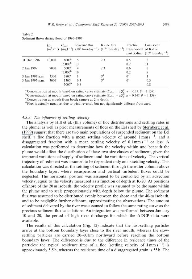
The flux estimates during the flood of January 1997 could only be accomplished bythe indirect method, due to the lack of moored measurements in the plume. Theresults of these calculations are shown in Table 2. Using the rather uncertainestimates based on Eq. (5), approximately 20–60% of the sediment remained in theplume at the K-line during the peak flow measurements on December 31 andJanuary 2. These proportions are similar to the 1998 observations, indicating that inboth 1997 and 1998, more than half of the sediment discharged from the river wasdelivered to the bottom boundary layer to the south of the K-line.

Fig. 11. Estimated sediment flux during 1998 at the river mouth (shading) and at the K-line (solid line).

Estimates at the K-line from helicopter survey data are indicated by circles. The upper bound on the

rivermouth flux estimate is based on Syvitski and Morehead (1999) and the lower bound uses a value

a ¼ 0:4 in Eq. 5. The difference between the flux at the river mouth and the flux at the K-line is an estimate

of the sediment that settled out of the plume to the south of the K-line.

W.R. Geyer et al. / Continental Shelf Research 20 (2000) 2067–20932088

4.3.3. The influence of settling velocityThe analysis by Hill et al. (this volume) of floc distributions and settling rates in

the plume, as well as prior measurements of flocs on the Eel shelf by Sternberg et al.(1999) suggest that there are two main populations of suspended sediment on the Eelshelf, a floc fraction with a mean settling velocity of around 1mm sÿ 1, and adisaggregated fraction with a mean settling velocity of 0.1mm sÿ 1 or less. Acalculation was performed to determine how the velocity within and beneath theplume would affect the distribution of these two size classes of sediment, given thetemporal variations of supply of sediment and the variations of velocity. The verticaltrajectory of sediment was assumed to be dependent only on its settling velocity. Thiscalculation was directed at the settling of sediment through the water column abovethe boundary layer, where resuspension and vertical turbulent fluxes could beneglected. The horizontal position was assumed to be controlled by an advectionvelocity, equal to the velocity measured as a function of depth at K-20. At positionsoffshore of the 20m isobath, the velocity profile was assumed to be the same withinthe plume and to scale proportionately with depth below the plume. The sedimentflux was assumed to be distributed evenly between the shore and the 40-m isobath,and to be negligible further offshore, approximating the observations. The amountof sediment delivered by the river was assumed to follow the same rating curve as theprevious sediment flux calculations. An integration was performed between January10 and 20, the period of high river discharge for which the ADCP data wereavailable.

The results of this calculation (Fig. 12) indicate that the fast-settling particlesarrive at the bottom boundary layer close to the river mouth, whereas the slow-settling particles are carried 20–60 km northward before reaching the bottomboundary layer. The difference is due to the difference in residence times of theparticles: the typical residence time of a floc (settling velocity of 1mm sÿ 1) isapproximately 5.5 h, whereas the residence time of a disaggregated grain is 55 h. The

Table 2

Sediment fluxes during flood of 1996–1997

Qf

(m3 sÿ 1)

Criver

(mg lÿ 1)

Riverine flux

(106 tons dayÿ 1)

K-line flux

(106 tons dayÿ 1)

Fraction

transported

past K-line

Loss south

of K-line

(106 tons dayÿ 1)

31 Dec 1996 10,000 6000a 5 2.3 0.5 3

15,000b 13 0.2 11

2 Jan 1997 9000 5000a 4 2.3 0.6 2

13,000b 10 0.2 8

3 Jan 1997 a.m. 3500 3800c 1 0d 0d 1

3 Jan 1997 p.m. 3000 1300a 0.3 0d 0d 0.3

3000b 0.8 0.8

aConcentration at mouth based on rating curve estimate (Criver ¼ aQbf , a ¼ 0:14;b ¼ 1:139).

bConcentration at mouth based on rating curve estimate (Criver ¼ aQbf ; a ¼ 0:347; b ¼ 1:139).

cConcentration at mouth from bottle sample at 2-m depth.dFlux is actually negative, due to wind reversal, but not significantly different from zero.

W.R. Geyer et al. / Continental Shelf Research 20 (2000) 2067–2093 2089

peaks that occur at different locations along the shelf reflect the contributions ofindividual flood events and the details of the flow immediately following each event.

The above calculations of flux past the K-line indicate that 30–40% of thesediment is carried more than 10-km north of the mouth. This calculation indicatesthat most of the sediment that is transported that far is disaggregated, and that thefraction that is trapped to the south represents the floc fraction. The settling of60–70% of the sediment to the south of the K-line could be explained ifapproximately that fraction of sediment is flocculated within the plume.

4.3.4. Delivery of sediment to the flood depositWheatcroft et al. (1997) determined that the flood deposit from the 1995 flood lies

between the 50- and 90-m isobaths. The 1997 flood produced a similar distribution ofsediment deposition, with an integrated mass of approximately 7 million metric tons(Wheatcroft and Borgeld, this volume). These observations indicate that of about 21million tons delivered from the river in 1997, 13 million tons fell out of the plume tothe south of the K-line and 8 million tons were transported in the plume to the north.However, a negligible fraction was transported offshore, beyond the 50-m isobath,within the plume. Thus, the sediment transport by the plume clearly did not deliverthe sediment to the flood deposit.

In spite of the large mass of riverine sediment delivered to the inner shelf,sedimentological data indicate that there is little mud deposition on the inner shelf,based on sediment grain size analysis (Wheatcroft and Borgeld, this volume). Thissuggests that either resuspension within the bottom boundary layer preventedsediment from settling, or that resuspension following the discharge eventsremobilized the sediment to be deposited elsewhere. There was substantialresuspension observed over the inner shelf (Figs. 7 and 8) following major floods,undoubtedly of fine sediment based on the vertical distribution of sediment and theintensity of the OBS signal. The near-bottom concentrations were not high enough

Fig. 12. Calculated estimates of the along-shelf distribution of sediment of sediment delivered from the

Eel River between January 10 and January 20, 1998, assuming settling velocities of 1mms-1 (solid line) and

0.1mm s-1 (dashed line).

W.R. Geyer et al. / Continental Shelf Research 20 (2000) 2067–20932090

on January 15 to account for the sediment that had been trapped there, so a majorfraction must have settled (unless it was rapidly transported seaward in the bottomboundary layer; see Traykovski et al., this volume). Thus, it appears that thesediment formed an ephemeral deposit on the inner shelf before being transported tothe flood deposit and elsewhere (cf, Wheatcroft and Borgeld, this volume).

Intense bottom resuspension on the inner shelf due to wave orbital motions ismore than adequate to remobilize this temporary inner shelf mud layer (Harris,1999; Traykowski et al., this volume). Once remobilized, the sediment may have beentransported offshore within the bottom boundary layer, driven by the excess densityof a layer of fluid mud (Traykowski et al., this volume). According to the rough massbalance presented here, approximately half of the mass of sediment that fell out ofthe plume to the south of the K-line could account for the sediment that accumulatedin the offshore flood deposit. The remainder of the sediment may have beendispersed in the seaward direction or transported along the coast. Observations byAlexander and Simoneau (1999) of sediment deposition on the continental slope tothe north of the flood deposit suggest that there is widespread northward dispersal ofEel River sediment. The Eel Canyon to the south may be an offshore conduit for EelRiver sediment as well, based on recent observations by Mullenbach and Nittrouer(personal communication, 1999).

5. Conclusions

Large floods of the Eel River produce a narrow, energetic plume that transportsfresh water and sediment rapidly to the north over the inner shelf. The trajectory andspeed of the plume are due both to the direct influence of the momentum andbuoyancy of the outflow and the forcing by southerly winds. The nearly along-shelforientation of the mouth of the river causes the momentum of the river outflow to bedirected primarily along-shelf, which provides an important source of momentum tothe plume and limits its offshore extent. Periods of high discharge are correlated withsoutherly winds, due to the association of low-pressure systems with highprecipitation in the watershed. Strong southerly winds produce downwelling-favorable conditions over the shelf, augmenting the northward velocity of the plumeand further narrowing of the plume. Tides perturb the along-shelf transport andpossibly cause mixing at the mouth of Humboldt Bay, but they do not significantlyalter the net transport of the plume. The plume is thin (5–7m vertically), even duringstrong winds, attesting to the stabilizing influence of the large buoyancy flux.

The sediment transport by the plume is strongly dependent on plume speed andthe settling rate of the suspended particles. During strong southerly wind conditions,the plume carries unaggregated, slowly settling particles more than 60-km north ofthe river mouth, whereas coarser grains and flocculated particles fall to the bottomboundary layer within 1-10-km of the mouth. During relatively infrequentoccurrences of northerly winds, the plume slows down, and even the fine sedimentsettles close to the mouth. There is no significant offshore transport of sediment bythe plume during either northerly or southerly winds, thus the plume does not

W.R. Geyer et al. / Continental Shelf Research 20 (2000) 2067–2093 2091

provide the offshore transport of sediment required to reach the mid-shelf flooddeposit. Rather, the plume delivers the sediment to the bottom boundary layer onthe inner shelf, possibly leading to the formation of an ephemeral mud deposit. Thusthe seaward transport of sediment into the mid-shelf flood deposits and off the shelfmust occur due to processes within the bottom boundary layer, including wave-induced resuspension and possibly the gravity-driven transport of dense suspensions(Traykowski et al., this volume; Ogston et al., this volume).

Acknowledgements

The authors thank Debbie Mondeel for coordinating the rapid response study,and the US Coast Guard Group Humboldt Bay for performing flights on shortnotice and in extreme weather conditions. Thanks to J. Lynch and J. Irish forimplementation of the moored measurements. This work was supported by ONR’sSTRATAFORM program, grant #N00014-97-10134. Woods Hole OceanographicInst. contribution number 10005.

References

Alexander, C.R., Simoneau, A.M., 1999. Spatial variability in sedimentary processes on the Eel

continental slope. Marine Geology 154, 243–254.

Allen, J.S., 1980. Models of wind-driven currents on the continental shelf. Annual Reviews of Fluid

Mechanics 12, 289–433.

Armi, L., 1986. The hydraulics of two flowing layers with different densities. Journal of Fluid Mechanics

163, 27–58.

Borgeld, J.C., Hughes Clark, J.E., Goff, J.A., Mayer, L.A., Curtis, J.A., 1999. Acoustic backscatter of the

1995 flood deposit on the Eel shelf. Marine Geology 154, 197–210.

Brown, W.M., Ritter, J.R., 1971. Sediment transport and turbidity in the Eel River basin, California. US

Geological Survey Water-Supply Paper 1986, 70pp.

Chao, S.-Y., Boicourt, W.C., 1986. The onset of estuarine plumes. Journal of Physical Oceanography 16,

2137–2149.

Chao, S.-Y., 1988a. River-forced estuarine plumes. Journal of Physical Oceanography 18, 72–88.

Chao, S.-Y., 1988b. Wind-driven motion of estuarine plumes. Journal of Physical Oceanography 18, 1144–

1166.

Fong, D.A., 1998. Dynamics of freshwater plumes: observations and numerical modeling of the wind-

forced response and alongshore freshwater transport. Ph. D. Thesis, MIT/WHOI, 98-16, 172 pp,

in press.

Garvine, R.W., 1982. A steady state model for buoyant surface plume hydrodynamics in coastal waters.

Tellus 34, 293–306.

Garvine, R.W., 1987. Estuary plumes and fronts in shelf waters: a layer model. Journal of Physical

Oceanography 17, 1877–1896.

Garvine, R.W., 1995. A dynamical system of classifying buoyant coastal discharges. Continental Shelf

Research 15, 1585–1596.

Geyer, W.R., Beardsley, R.C., Candela, J., Lentz, S.J., Limeburner, R., Johns, W.E., Castro, B.M.,

Soares, I.D., 1996. Physical oceanography of the Amazon Shelf. Contintental Shelf Research 16,

575–616.

W.R. Geyer et al. / Continental Shelf Research 20 (2000) 2067–20932092

Largier, J.L., Magnell, B.A., Winant, C.D., 1993. Subtidal circulation over the northern California shelf.

Journal of Geophysical Research 98 (18), 147–18, 179.

Harris, C.K., 1999. The importance of advection and flux divergence in the transport and redistribution of

continental shelf sediment. Ph.D. Thesis, University of Virginia Department of Environmental Sciences,

155pp.

Hill, P.S., Milligan, T.G., Geyer, W.R. Controls on effective settling velocity of suspended sediment in the

Eel River flood plume. Continental Shelf Research 20, 2095–2111.

Kineke, G.C., Sternberg, R.W., 1992. Measurements of high concentration suspended sediments using the

Optical Backscatterance Sensor. Marine Geology 198, 253–258.

Kudrayavtsev, V.N., Soloviev, A.V., 1990. Slippery near-surface layer of the ocean arising due to daytime

solar heating. Journal of Physical Oceanography 20, 617–627.

Lentz, S.J., Winant, C.D., 1986. Subinertial currents on the southern California shelf. Journal of Physical

Oceanography 16, 1737–1750.

Lentz, S.J., Limeburner, R., 1995. The amazon River plume during AmasSeds: spatial characteristics and

salinity variability. Journal of Geophysical Research 100, 2355–2375.

Lentz, S., Guza, R.T., Elgar, S., Feddersen, F., Herbers, T.H.C., 1999. Momentum balances on the North

Carolina inner shelf. Journal of Geophysical Research 104, 18,205–18,226.

Milligan, T.G., Krank, K., 1991. Electro-resistance particle size analyzers. In: Syviski, J.P.M. (Ed.),

Principles, Methods and Applications of Particle Size Analysis. Cambridge University Press, New York,

pp. 109–118.

Milliman, J.D., Syvitski, J.P.M., 1992. Geomorphic/tectonic control of sediment discharge to the ocean:

the importance of small mountainous rivers. Journal of Geology 91, 1–21.

Morehead, M.D., Syvitski, J.P., 1999. River-plume sedimentation modeling for sequence stratigraphy:

application to the Eel margin, northern California. Marine Geology 154, 29–42.

Nash, D.B., 1994. Effective sediment-transporting discharge from magnitude-frequency analysis. Journal

of Geology 102, 79–95.

Ogston, A., Cacchione, D.A., Sternberg, R.W., Kineke, G.C. Observations of storm and river flood-driven

sediment transport on the Northern California continental shelf. Continental Shelf Research 20,

2141–2162.

Rennie, S.E., Largier, J.L., Lentz, S.J., 1999. Observations of a pulsed buoyancy current downstream of

Chesapeake Bay. Journal of Geophysical Research 104, 18,227–18,240.

Sommerfield, C.K., Nittrouer, C.A., 1999. Modern accumulation rates and a sediment budget for the Eel

shelf: a flood dominated depositional environment. Marine Geology 154, 227–242.

Sternberg, R.W., Berhane, I., Ogston, A.S., 1999. Measurement of size and settling velocity of suspended

aggregates on the northern California continental shelf. Marine Geology 154, 43–54.

Syvitski, J.P., Morehead, M.D., 1999. Estimating river-sediment discharge to the ocean: application to the

Eel margin, northern California. Marine Geology 154, 13–28.

Traykovski, P., Geyer, W.R., Irish, J.D., Lynch J.F. The role of wave-induced density-driven fluid mud

flows for cross-shelf transport on the Eel River continental shelf. Continental Shelf Research 20, 2113–

2140.

Wheatcroft, R.A., Sommerfield, C.K., Drake, D.E., Borgeld, J.C., Nittrouer, C.A., 1997. Rapid and

widespread dispersal of flood sediment on the northern California margin. Geology 25, 163–166.

Wheatcroft, R.A., Borgeld, J.C. Oceanic flood deposits on the northern California shelf: large scale

distribution and small-scale physical properties. Continental Shelf Research 20, 2163–2190.

Yankovsky, A.E., Chapman, D.C., 1997. A simple theory for the fate of buoyant coastal discharges.

Journal of Physical Oceanography 27, 1386–1401.

W.R. Geyer et al. / Continental Shelf Research 20 (2000) 2067–2093 2093