1

Environmental

Sciences

Atmospheric Processes

Plume Behaviour

Paper No: 8 Atmospheric Processes

Module: 9 Plume Behaviour

Development Team

Principal Investigator

&

Co- Principal Investigator

Prof. R.K. Kohli

Prof. V.K. Garg &Prof. Ashok Dhawan

Central University of Punjab, Bathinda

Paper Coordinator

Dr. Sunayan Saha

Scientist, ICAR-National Institute of Abiotic Stress Management,

Baramati, Pune

Content Writer Dr. Puneeta Pandey

Central University of Punjab, Bhatinda

Content Reviewer Dr. Dhanya M S

Central University of Punjab, Bhatinda

Anchor Institute

Central University of Punjab

2

Environmental

Sciences

Atmospheric Processes

Plume Behaviour

Description of Module

Subject Name Environmental Sciences

Paper Name Atmospheric Processes

Module Name/Title Plume Behaviour

Module Id EVS/AP-VIII/9

Pre-requisites Basic knowledge of elementary physics and computers

Objectives

To familiarize the reader with the concept of atmospheric stability

To understand plume behaviour and its types

To understand point-source Gaussian Dispersion model

Keywords Stability, Lapse Rate, Plume, Model, Gaussian, Line, Area

3

Environmental

Sciences

Atmospheric Processes

Plume Behaviour

TABLE OF CONTENTS

1. Aim of the module

2. Introduction

3. Atmospheric stability

3.1. Lapse rate

3.2. Types of stability

4. Plume behaviour

5. Air quality models

5.1 Types of air quality models

5.2 Examples of air quality models

6. The point source Gaussian dispersion model

6.1 Line source dispersion model

6.2 Area source dispersion model

6.3 Advanced Gaussian models

6.4 Advantages and limitations of Gaussian model

6.5 Examples of advanced Gaussian models

7. Conclusions

1. Aim of the module

The aim of the present module is:

To familiarize the reader with the concept of atmospheric stability

To understand plume behaviour and its types

4

Environmental

Sciences

Atmospheric Processes

Plume Behaviour

To understand point-source Gaussian Dispersion model

2. Introduction

In meteorology, we generally study about the movement of air mass (generally horizontal) from one

place to the other. Many times, the particles in the air parcel get transported vertically by a process

called turbulent diffusion or eddy diffusion (Daly and Zannetti, 2007). This horizontal and vertical

motion of air parcels is responsible for various atmospheric processes such as cloud formation and

plume behaviour. In this module, we shall study the concept of atmospheric stability and lapse rate;

the types of stability, plume behaviour of pollutants released from stack and air quality models. The

model shall, however, be limited to point-source Gaussian dispersion model and its application to

linear and area source models.

3. Atmospheric stability

The resistance of the atmosphere to vertical motion is called as atmospheric stability. An air parcel in

meteorology refers to an air mass having more or less uniform properties. An air parcel will expand

and cool as it rises and will compress and warm as it sinks. The reason behind this primarily is that as

the air parcel rises, it encounters lower pressure and vice-versa. If we assume that the process is

adiabatic, which implies that no exchange of energy of air parcel occurs with the environment; then as

the air parcel rises, it will expand and cool since the internal energy is used up during the process. The

term ‘adiabatic’ is derived from the Greek word ‘impassable’, implying a system which does not lose

or gain energy. Reverse process occurs when the air parcel sinks and internal energy is released during

sinking which warms up the air parcel.

3.1 Lapse rates

Lapse rate refers to the rate of change of temperature or pressure with height. In the atmosphere, this

rate of change of temperature with altitude is called as Environmental Lapse Rate (ELR) and

corresponds to 6.5°C km-1. This implies that for every kilometer increase in altitude, temperature drops

5

Environmental

Sciences

Atmospheric Processes

Plume Behaviour

by 6.5°C. Actual vertical temperature gradients in the atmosphere are thus highly variable, and can

even show an increase in temperature with height, a situation known as a temperature inversion.

If a dry air parcel is considered instead of environment, a linear relationship exists between

temperature and altitude for rising or sinking air parcel, which is known as Dry Adiabatic Lapse Rate

(DALR) and is equal to 9.8°C km-1.

When condensation or evaporation occurs in the air, however, lapse rates of rising or falling air differ

from DALR value due to effect of latent heat. As is obvious, latent heat is released by condensation

and consumed by evaporation of water. This leads to change in adiabatic lapse rate since energy

released by condensation compensates the rate of cooling of rising air. This modified lapse rate is

termed the Saturated Adiabatic Lapse Rate (SALR) or Moist Adiabatic Lapse Rate (MALR). Since the

concentration of water vapour in air varies from place to place, SALR is non-linear in nature. The

average value of SALR in the troposphere is generally 6°C km-1.

3.2 Types of stability

Stability of the atmosphere is affected by:

Temperature of the surrounding environment

Temperature of the air parcel

Accordingly, the types of stability are as follows:

A. Stable: If the air parcel is displaced vertically, and it returns back to its original position, the

atmosphere is said to be stable. It usually occurs when the ELR is less than the Adiabatic Lapse Rate

(ALR), a phenomenon occurring generally during temperature inversion. If such a parcel of air is

uplifted, it will cool to lower temperatures than its new surroundings along the ALR; thus, becoming

denser than the surroundings. Hence the air parcel will tend to fall back to its original level.

B. Neutrally stable: If the parcel is displaced vertically, it will acquire a new position and continue to

remain in its new position. This generally occurs when ELR is more or less equal to ALR.

6

Environmental

Sciences

Atmospheric Processes

Plume Behaviour

C. Unstable: If the parcel is displaced vertically, it will accelerate away from its original position in

the direction of the initial displacement. Such unstable condition occurs when ELR is greater than

ALR.

4. Plume behaviour

Plume behaviour refers to the dispersal pattern of gaseous pollutants in atmosphere depending upon

wind conditions, atmospheric stability and vertical temperature profile. It shows seasonal as well as

diurnal variations. Accordingly, there are various types of plume discussed below and represented

diagrammatically in figure 1.

Figure 1: Plume behaviour

7

Environmental

Sciences

Atmospheric Processes

Plume Behaviour

A. Looping plume: It takes place when the atmosphere is very unstable, wind speed is greater than 10

ms-1, has super-adiabatic lapse rate and is accompanied with solar heating. It follows a wave like

pattern and provides high degree of mixing at lower levels, sometimes reaching the ground.

B. Fumigation: It occurs when plume reaches the ground level along the length of the plume and is

caused by a super-adiabatic lapse rate beneath an inversion. The super-adiabatic lapse rate at the

ground level occurs due to the solar heating and is quite undesirable since the pollutants remain at

ground level. This condition is favoured by clear skies and light winds.

C. Coning plume: It results when the vertical air temperature gradient occurs between dry adiabatic

and isothermal, the air being slightly unstable with some horizontal and vertical mixing occurring.

Coning is most likely to occur during cloudy or windy periods.

D. Fanning plume: They spread out horizontally but do not mix vertically. Fanning plumes take place

when inversion condition exists in atmosphere, that is, the air temperature increases with altitude. The

plume rarely reaches the grounds level unless the inversion is broken by surface heating or a

topographical barrier such as a hill. At night, with light winds and clear skies, fanning plumes are quite

common.

E. Lofting plume: It diffuses upward but not downwards and occurs when there is a super-adiabatic

layer above a surface inversion. A lofting plume will generally not reach the ground surface, so there

is less pollution at ground level.

F. Trapping: This condition is accompanied by weak lapse below inversion aloft.

5. Air quality models

Air quality models use mathematical algorithms to simulate the behaviour of air pollutant as they

disperse in the atmosphere and the physical and chemical processes they undergo during dispersion.

Usually these models simulate the behaviour of primary pollutants and occasionally the secondary

pollutants formed due to chemical reactions of primary pollutants in the atmosphere. Although the

inputs for different air quality models vary according to model requirements, certain parameters such

as wind speed and direction, temperature and humidity find importance in almost all models. Thus,

these models find wide application in agencies involved with management of air quality, site-

8

Environmental

Sciences

Atmospheric Processes

Plume Behaviour

suitability analysis for establishment of new source as well as predicting future concentration of

pollutants.

5.1 Types of air quality models

Air quality models can be categorized into four classes.

A. Gaussian: Used for estimating the ground-level impact of non-reactive pollutants from stationary

sources in a smooth terrain

B. Numerical: Used for estimating the impact of reactive and non-reactive pollutants in complex

terrain

C. Statistical: Employed in situations where physical or chemical processes are not well understood

D. Physical: Involves experimental investigation of source impact in a wind tunnel facility

5.2 Examples of air quality models

Some examples of air quality models are as follows:

A. Dispersion models: These models estimate the concentration of pollutants at specified ground-

level receptors in the vicinity of an emissions source. These air quality models are used to determine

compliance with National Ambient Air Quality Standards (NAAQS) and other regulatory

requirements such as New Source Review (NSR) and Prevention of Significant Deterioration (PSD)

regulations.

B. Photochemical models: These models estimate pollutant concentrations and deposition of both

inert and chemically reactive pollutants such as ozone, particulate matter (PM) and mercury over large

spatial scales and are used in regulatory assessments.

C. Receptor models: These models use chemical and physical characteristics of gases and particles

measured at source and receptor to identify and quantify contribution of atmospheric source to

9

Environmental

Sciences

Atmospheric Processes

Plume Behaviour

receptor concentrations.

6. The point source Gaussian dispersion model

How do pollutants behave in the atmosphere once they have been emitted? How may we predict their

concentrations in the atmosphere? How can we predict the improvement in air quality that must be

achieved when new sources are proposed? To help answer these questions, computer models are used.

These models use the following inputs:

Predicted emissions

Smokestack heights

Wind data

Atmospheric temperature profiles

Ambient temperatures

Solar insolation

Local terrain features

The point source Gaussian plume model is based on the assumption that the time-averaged pollutant

concentration downwind from a source can be modeled using a normal or Gaussian distribution curve.

The basic Gaussian dispersion model applies to:

Single point Source: Smokestack

Line Source: Emissions from motor vehicles along a highway

Area Sources: These can be modeled as large number of point sources

10

Environmental

Sciences

Atmospheric Processes

Plume Behaviour

Figure 2: The instantaneous plume boundary and a time-averaged plume envelope of a Gaussian dispersion

model

Consider a single point source, for example, a smokestack. The coordinate system shows a cross-

section of the plume, with ‘z’ representing vertical direction and ‘x’ is the distance directly downwind

from the source. If we were to observe the plume at any particular instant, it might have some irregular

shape, such as the outline of the looping plume shown. A few minutes later, however, the plume might

have an entirely different boundary. Thus, time-averaged plume envelope develops over a period of

time.

Since stack emissions have some initial upward velocity and buoyancy, it might be some distance

downwind before the plume envelope might begin to look symmetrical about a centerline. The

centerline is generally somewhat above the actual stack height. The highest concentration of pollution

would be along the centerline, with decreasing concentrations as the distance from this centerline

increases. The Gaussian plume model assumes that the pollutant concentration follows a normal

distribution about this centerline in both horizontal and vertical directions. It also treats emission as

they came from a virtual point source along the plume centerline, at an effective stack height H.

11

Environmental

Sciences

Atmospheric Processes

Plume Behaviour

The Gaussian point source dispersion equation relates average, steady state pollutant concentrations to

the source strength, wind speed, effective stack height and atmospheric conditions. Its form can be

derived from the basic considerations involving gaseous diffusion in three-dimensional space. The

following assumptions are incorporated into the analysis:

The rate of emissions from the source is constant.

The wind speed is constant both in time and with elevation.

The pollutant is conservative, i.e., it is not lost by decay, chemical reaction or deposition. On

hitting the ground, all is reflected and none is absorbed.

The terrain is relatively flat, open country.

The three-dimensional coordinate system has the stack at the origin, with distance directly downwind

given by x, distance off the downwind axis specified by y, and elevation given by z. Since our concern

is people and ecosystems at ground level, the following Gaussian plume equation applies only for z=0.

……………………….. (1)

Where, C(x,y) = concentration at ground level at the point (x,y), µg m-3

y= horizontal distance from the plume centerline, m

Q= emission rate of pollutants, µg/s

H= effective stack height, m (H=h+Δh, where, h= actual stack height, and Δh= plume rise)

uH = average wind speed at the effective height of the stack, ms-1

σy = horizontal dispersion coefficient (standard deviation), m

σz = vertical dispersion coefficient (standard deviation), m

From Equation (1), the following points are clear:

Ground level pollution concentration is directly proportional to the source strength Q, so that

the amount of source reduction required to achieve a desired decrease in downwind

concentration can be determined.

12

Environmental

Sciences

Atmospheric Processes

Plume Behaviour

Ground level pollution decreases when taller stacks are used, although relationship is not

linear.

There is no explicit relationship between emission rate, Q, and downwind distance, x.

Downwind concentration appears to be inversely proportional to the wind speed, and is slightly

modified by the dependence of plume rise Δh on wind speed.

The Gaussian plume equation is based on both theory and actual measured data, and its

prediction is accurate to ±50%. However, it is still very useful due to its universal acceptance,

easy to use and allows comparison between estimates made by different modelers in varying

situations.

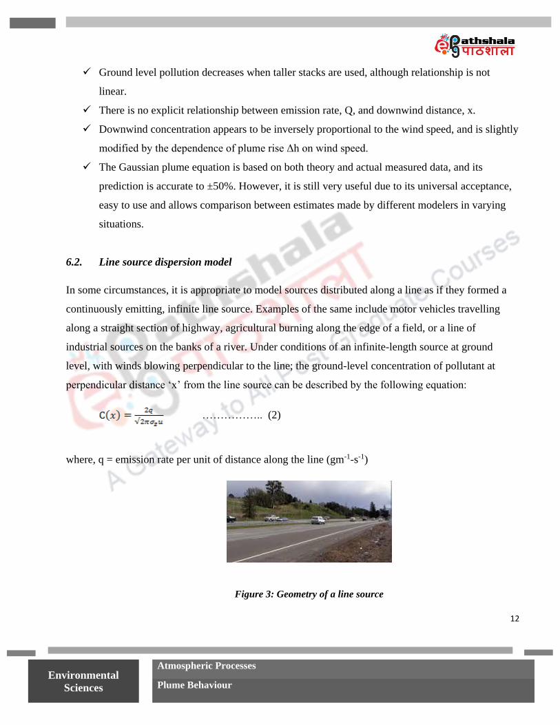
6.2. Line source dispersion model

In some circumstances, it is appropriate to model sources distributed along a line as if they formed a

continuously emitting, infinite line source. Examples of the same include motor vehicles travelling

along a straight section of highway, agricultural burning along the edge of a field, or a line of

industrial sources on the banks of a river. Under conditions of an infinite-length source at ground

level, with winds blowing perpendicular to the line; the ground-level concentration of pollutant at

perpendicular distance ‘x’ from the line source can be described by the following equation:

…………….. (2)

where, q = emission rate per unit of distance along the line (gm-1-s-1)

Figure 3: Geometry of a line source

13

Environmental

Sciences

Atmospheric Processes

Plume Behaviour

6.3. Area source dispersion models

For distributed sources, various methodologies can be applied to estimate pollutant concentrations. If

there are a modest number of point sources, it is reasonable to use the point source Gaussian plume

equation for each source to predict its individual contribution. Then, by superposition, find the total

concentration at a given location by summing the individual contributions. Another approach could be

multiple use of Gaussian line-source equation. By dividing an area into a series of parallel strips and

then treating each strip as a line source, the total concentration on any strip can be estimated.

Another approach involves estimating pollutant concentrations over an area, such as a city, by using

the box model concept. Consider the airshed over an urban area to be represented by a rectangular box

with base dimensions L and W and height H. The box is oriented such that wind speed ‘u’ is normal to

one side of the box. The height of the box is determined by mixing depth and emissions per unit area

will be represented by qs (gm-2s-1).

Consider the air blowing into the box on the upwind side to have pollutant concentration Cin, and

assume that no pollutant is lost from the box along the sides parallel to the wind or from the top. It is

assumed that the pollutants are rapidly and completely mixed in the box creating a uniform average

concentration C. Also the pollutants are assumed to be conservative in nature, i.e., they do not react,

decay or fall out of air stream.

14

Environmental

Sciences

Atmospheric Processes

Plume Behaviour

Figure 4: Box model for an airshed over a city. Emissions per unit area are given by qs, pollutants

are assumed to be uniformly mixed in the box with concentration C, and upwind of the box, the

concentration is Cin.

Thus, the amount of pollutants in the box is the volume of the box times the concentration, LWHC.

The rate at which air is entering and leaving the box is the area of either end times the windspeed,

WHu, so the rate at which pollutants is entering the box is WHuCin. The rate at which it leaves the box

is WHuC. If we assume the pollutant is conservative, then the mass balance equation for the box may

be written as:

(Rate of change of pollution in the box) = (Rate of pollution entering the box) - (Rate of pollution

leaving the box)

Or,

………………………(3)

Cin= concentration in the incoming air, mg m-3

qs= emission rate per unit of area, mg m-2s-1

H= mixing height, m

15

Environmental

Sciences

Atmospheric Processes

Plume Behaviour

L= length of airshed, m

W= width of airshed, m

u= average windspeed against one edge of the box, m s-1

The steady state solution to equation (3) can be obtained by setting dC/dt = 0, so that

………………………….. (4)

Equation (3) can also be solved to obtain the time-dependent increase in pollution above the city.

Letting C(0) be the concentration in the airshed above the city at time t=0, the solution becomes

…………………………. (5)

If it is assumed that incoming wind blows no pollution into the box, and if the initial concentration in

the box is zero, then equation (5) becomes

………….. (6)

When t = L/u, the exponential function becomes e-1 and the concentration reaches about 63% of its

final value. This is called time constant, the ventilation time, the residence time, or the e-folding time.

6.4. Advantages and limitations of Gaussian model

Advantages:

Fast response time

Easy to calculate

Can be applied to real-time GIS-based decision support software

Can be successfully used for a wide range of studies of air quality in urban and industrial areas

Limitations:

16

Environmental

Sciences

Atmospheric Processes

Plume Behaviour

Does not incorporate meteorological parameters

Unsatisfactory performance in industrial incidents such as Bhopal and Chernobyl disaster

6.5. Examples of advanced Gaussian models

I. AERMOD: It is an open-source Gaussian air dispersion model developed by the US Environmental

Protection Agency (EPA) to carry out impact studies of planned or existing industrial sites. It has built-

in models to handle complex terrain and urban boundary layer. Besides, although AERMOD uses the

steady-state approximation for the flow and the source, it can be used within 10–100 km distance

using its meteorological pre-processor, AERMET.

II. Complex Terrain Dispersion Model (CTDM) - This has also been developed by EPA to estimate

concentration patterns in mountain regions.

III. ADMS: The ADMS (Atmospheric Dispersion Modeling System) model has been developed in

Europe for air quality simulations. It incorporates meteorological effects like coastal circulations,

complex terrain, deposition processes and radioactive decay.

IV. CERC: UK Met Office and Cambridge Environmental Research Consultants (CERC) also

developed the ADMS-Urban module that aims to provide air quality forecasts for cities.

V. Other Gaussian models: There are several other Gaussian models used for impact and health risk

studies such as CALINE3 (for highway air pollution), OCD for coastal areas, BLP and ISC for

industrial sites or ALOHA for accidental and heavy gas releases. They are widely used by authorities,

environmental protection organizations and industry investigations.

7. Conclusions

At the end of this module, the reader shall be able to understand the types of atmospheric stability,

how it affects the plume behaviour, types and examples of air quality models with special reference to

point-source Gaussian dispersion model. These models find wide application in management of air

17

Environmental

Sciences

Atmospheric Processes

Plume Behaviour

quality as well as predicting future scenarios of air quality. This is relevant due to rising air pollution

levels all over the globe and provides a fast, simplistic and cost-effective solution at local level,

especially at sites where air quality monitoring is difficult due to experimental difficulties.

References

Daly, A. and P. Zannetti. 2007. Air Pollution Modeling – An Overview. Chapter 2 of AMBIENT AIR

POLLUTION (P. Zannetti, D. Al-Ajmi, and S. Al-Rashied, Editors). Published by The Arab School

for Science and Technology (ASST) (http://www.arabschool.org.sy) and The EnviroComp Institute

(http://www.envirocomp.org/).

Gilbert M. Masters & Wendell P. Ela (2003). Introduction to Environmental Engineering. Prentice

Hall.

P. Venugopala Rao (2002). Textbook of Environmental Engineering. PHI Learning Pvt. Ltd., pp. 184

https://www.epa.gov/scram/modeling-applications-and-tools

https://www.epa.gov/scram/photochemical-modeling-applications

https://www.epa.gov/scram/photochemical-modeling-tools

https://www.epa.gov/scram/dispersion-modeling-applications

https://www.epa.gov/scram/dispersion-modeling-applications

https://www.epa.gov/scram/multipollutant-modeling-applications

https://www.epa.gov/scram/air-quality-models

https://www.epa.gov/scram/meteorological-data-and-processors

https://www3.epa.gov/scram001/dispersionindex.htm

18

Environmental

Sciences

Atmospheric Processes

Plume Behaviour

http://elte.prompt.hu/sites/default/files/tananyagok/AtmosphericChemistry/ch10s03.html

http://people.math.sfu.ca/~stockie/atmos/paper.pdf

https://www.ready.noaa.gov/READY_gaussian.php

http://www.rrcap.ait.asia/male/Documents/manual/national/04Chapter4.pdf

http://nptel.ac.in/courses/Webcourse-contents/IIT-

Delhi/Environmental%20Air%20Pollution/air%20pollution%20(Civil)/Module-4/1.htm

http://site.iugaza.edu.ps/afoul/files/2010/02/chapter_7.pdf

http://elte.prompt.hu/sites/default/files/tananyagok/AtmosphericChemistry/ch10s03.html

http://atoc.colorado.edu/~saraht/atoc1050/Lecture_Notes/chapter6-notes.pdf

------------------------------------------------------------------------------------------