BSc Chemistry - e-PG Pathshala

____________________________________________________________________________________________________

BUSINESS ECONOMICS

PAPER NO. : 2, APPLIED BUSINESS STATISTICS

MODULE NO. : 24, ONE WAY ANOVA

Subject BUSINESS ECONOMICS

Paper No and Title 2, Applied Business Statistics

Module No and Title 24, One Way ANOVA

Module Tag BSE_P2_M24

____________________________________________________________________________________________________

BUSINESS ECONOMICS



TABLE OF CONTENTS

1. Learning Outcomes

2. Introduction

3. One Way ANOVA

3.1 Concept of One Way ANOVA

3.1.1 Assumptions for application of ANOVA

3.2 Model for One Way ANOVA

3.3 Hypothesis Test for One Way ANOVA

4. Learning One Way ANOVA through Example

4.1 Learning One Way ANOVA

4.2 Limitation of ANOVA and further tests

5. Summary

____________________________________________________________________________________________________

BUSINESS ECONOMICS



1. Learning Outcomes

After studying this module, you shall be able to

Know how to test the difference between means of more than two samples.

Learn about One Way ANOVA.

Evaluate problems involving testing for difference in sample means due to one

characteristic.

Learn about which of the means are not similar with other means by two other means

namely Tuckey’s method and Least Significant Difference methods.

2. Introduction

One Way ANOVA

So far we have learnt to compare the means of two populations using the test of hypothesis or

more precisely the t-test for the difference between means. For example, if we wish to test the

hypothesis that the academic performance of first year students in college A is equal to or same as

the academic performance of first year students in college, we would set the null hypothesis as

Ho: Average marks of first year students in college A (A) is equal to average marks of first year

students in college B (B) at some specific level of significance say at 5%.

Mathematically writing

Null hypothesis : Ho : A = B

Alternative hypothesis : H1 : (A) (B)

But if we have to compare the academic performance of students in more than two colleges, we

cannot very easily use the above t-test. We require another method that can simultaneously test

the null hypothesis that the average marks obtained by students of three or more colleges is equal

as against the alternative hypothesis that the average marks obtained by the students of these three

or more colleges is not same (i.e.)

Ho : A = B = C = D…….

H1 : A B C D…….

Where C, D depicts average marks obtained by students of college C, D….. and so on. In the

above case we can use t-test of difference between means but will have to study only two colleges

at a time. Likewise if we wish to compare marks in four colleges A, B, C, D we will have to

perform the t-test 6 times (4C2) taking two colleges at a time. The combinations of colleges that

we will have to study would be AB, AC, AD, BC, BD and CD. You would appreciate that when

more than two populations are involved, the t-test for difference between means at a specific level

of significance say 5% becomes a very cumbersome process. If means of 4 samples are to be

____________________________________________________________________________________________________

BUSINESS ECONOMICS



compared with the null hypothesis that the average marks obtained by the students of 4 colleges is

same at 5% level of significance, then 4C2 =6 times the t test has to be conducted. Therefore, we

have an alternative in the form of ‘ANOVA’ called Analysis of Variance that helps us to test the

differences in means of more than two populations at a same time. Since this method examines

sample variances to establish whether difference in population means exists, it is known as the

“Analysis of Variance” method.

3. One Way ANOVA

3.1 Concept

The term ‘Analysis of Variance’ was coined by Prof. R.A. Fisher while studying agricultural data.

Here some selected plots of land were treated with different fertilizers to compare the average

crop yield of the land after fertilizer treatment. Post treatment the difference in crop yield was

noted and the causes of variation identified. The variation it was pointed, could be caused by i)

Assignable causes ii) chance causes.

The variation due to the first set of causes can be detected and measured whereas variation due to

chance causes is unpredictable and hence not measurable. Variation due to chance causes is

called ‘error’.

Let us consider an example where we wish to compare the impact of three different fertilizers

(namely A, B and C) on crop yield. To study this we might take a sample of 5 plots of agricultural

land where each fertilizer is applied. In this technique, the ‘experimental units’ are the plots of

land receiving fertilizer treatment which in our example are 5 x 3 = 15. The ‘factor’ is the

variable whose impact on experimental units we wish to study. In our example fertilizer treatment

is the factor and the 3 types of fertilizers A, B and C are the treatment or factor levels.

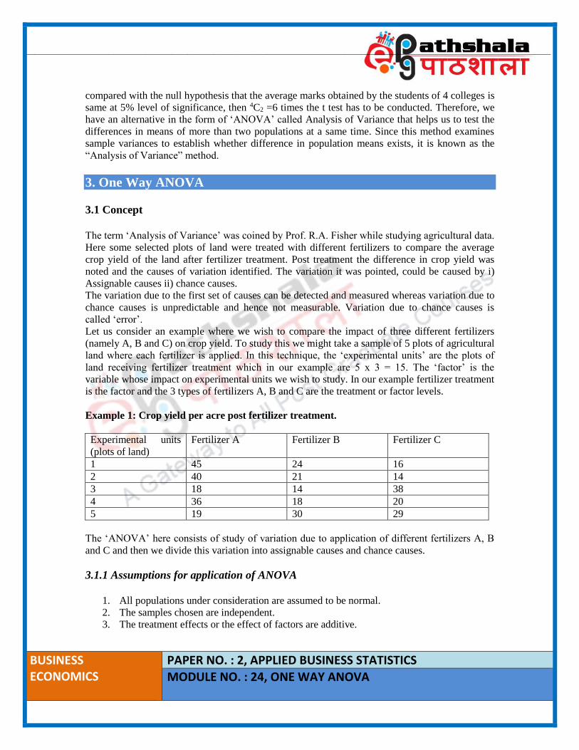
Example 1: Crop yield per acre post fertilizer treatment.

Experimental units

(plots of land)

Fertilizer A Fertilizer B Fertilizer C

1 45 24 16

2 40 21 14

3 18 14 38

4 36 18 20

5 19 30 29

The ‘ANOVA’ here consists of study of variation due to application of different fertilizers A, B

and C and then we divide this variation into assignable causes and chance causes.

3.1.1 Assumptions for application of ANOVA

1. All populations under consideration are assumed to be normal.

2. The samples chosen are independent.

3. The treatment effects or the effect of factors are additive.

____________________________________________________________________________________________________

BUSINESS ECONOMICS



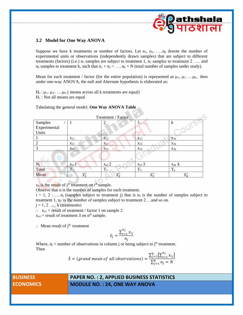
3.2 Model for One Way ANOVA

Suppose we have k treatments or number of factors. Let n1, n2, …..nk denote the number of

experimental units or observations (independently drawn samples) that are subject to different

treatments (factors) (i.e.) n1 samples are subject to treatment 1, n2 samples to treatment 2 ….. and

nk samples to treatment k, such that n1 + n2 + …..nk = N (total number of samples under study).

Mean for each treatment / factor (for the entire population) is represented as 1, 2 ….k, then

under one-way ANOVA, the null and Alternate hypothesis is elaborated as:

Ho : 1= 2= ….k ( means across all k treatments are equal)

H1 : Not all means are equal

Tabulating the general model: One Way ANOVA Table

Treatment / Factor

Samples /

Experimental

Units

1 2 3…… k

1 x11 x12 x13 x1k

2 x21 x22 x23 x2k

3 x31 x32 x33 x3k

Nj xn11 xn2 2 xn3 3 xnk k

Total T1 T2 T3 Tk

Mean 𝑥1̅̅ ̅ 𝑥2̅̅ ̅ 𝑥3̅̅ ̅ 𝑥4̅̅ ̅

xij is the result of jth treatment on ith sample.

Observe that n is the number of samples for each treatment.

i = 1, 2 ……nj (samples subject to treatment j) that is n1 is the number of samples subject to

treatment 1, n2 is the number of samples subject to treatment 2….and so on.

j = 1, 2 ….. k (treatments)

x21 = result of treatment / factor 1 on sample 2

xn3 = result of treatment 3 on nth sample.

Mean result of jth treatment

�̅�𝑗 =∑ 𝑥𝑖𝑗

𝑛𝑗

𝑖=1

𝑛𝑗

Where, nj = number of observations in column j or being subject to jth treatment.

Then

�̿� = (𝑔𝑟𝑎𝑛𝑑 𝑚𝑒𝑎𝑛 𝑜𝑓 𝑎𝑙𝑙 𝑜𝑏𝑠𝑒𝑟𝑣𝑎𝑡𝑖𝑜𝑛𝑠) =∑ [∑ 𝑥𝑖𝑗

𝑛𝑗

𝑖=1 ]𝑘𝑗=1

∑ 𝑛𝑗 = 𝑁𝑘𝑗=1

____________________________________________________________________________________________________

BUSINESS ECONOMICS



Here, double summation means that we sum all observation within each group (treatment) and

overall groups (samples).

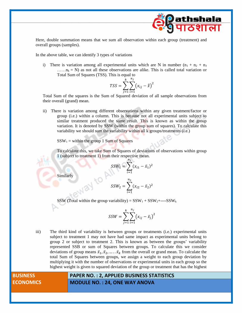
In the above table, we can identify 3 types of variations

i) There is variation among all experimental units which are N in number (n1 + n2 + n3

……nk = N) as not all these observations are alike. This is called total variation or

Total Sum of Squares (TSS). This is equal to

𝑇𝑆𝑆 = ∑ ∑(𝑥𝑖𝑗 − �̿�)2

𝑛𝑗

𝑖=1

𝑘

𝑗=1

Total Sum of the squares is the Sum of Squared deviation of all sample observations from

their overall (grand) mean.

ii) There is variation among different observations within any given treatment/factor or

group (i.e.) within a column. This is because not all experimental units subject to

similar treatment produced the same result. This is known as within the group

variation. It is denoted by SSW (within the group sum of squares). To calculate this

variability we should sum the variability within all k groups/treatments (i.e.)

SSW1 = within the group 1 Sum of Squares

To calculate this, we take Sum of Squares of deviations of observations within group

1 (subject to treatment 1) from their respective mean.

𝑆𝑆𝑊1 = ∑(𝑥𝑖1 − �̅�1)2

𝑛1

𝑖=1

Similarly

𝑆𝑆𝑊2 = ∑(𝑥𝑖2 − �̅�2)2

𝑛2

𝑖=1

SSW (Total within the group variability) = SSW1 + SSW2+----SSWk

𝑆𝑆𝑊 = ∑ ∑(𝑥𝑖𝑗 − �̅�𝑗)2

𝑛𝑗

𝑖=1

𝑘

𝑗=1

iii) The third kind of variability is between groups or treatments (i.e.) experimental units

subject to treatment 1 may not have had same impact as experimental units belong to

group 2 or subject to treatment 2. This is known as between the groups’ variability

represented SSB or sum of Squares between groups. To calculate this we consider

deviations of group means �̅�1, �̅�2, … . . �̅�𝑘 from the overall or grand mean. To calculate the

total Sum of Squares between groups, we assign a weight to each group deviation by

multiplying it with the number of observations or experimental units in each group so the

highest weight is given to squared deviation of the group or treatment that has the highest

____________________________________________________________________________________________________

BUSINESS ECONOMICS



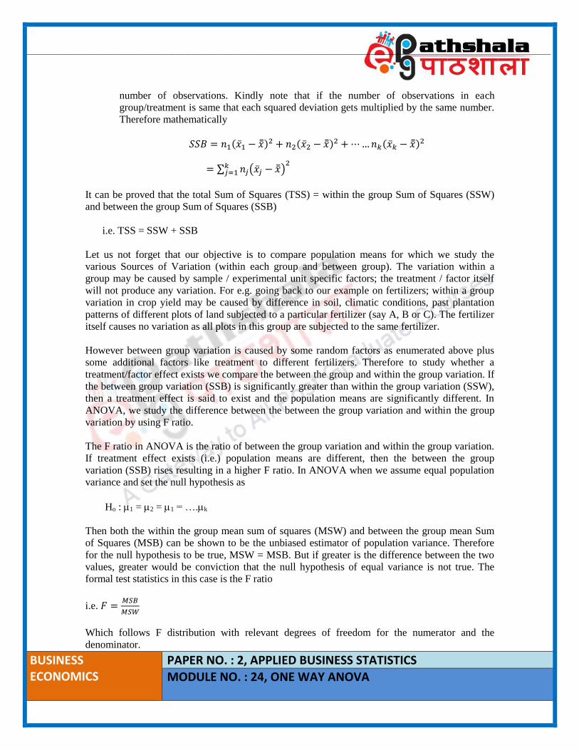
number of observations. Kindly note that if the number of observations in each

group/treatment is same that each squared deviation gets multiplied by the same number.

Therefore mathematically

𝑆𝑆𝐵 = 𝑛1(�̅�1 − �̿�)2 + 𝑛2(�̅�2 − �̿�)2 + ⋯ … 𝑛𝑘(�̅�𝑘 − �̿�)2

= ∑ 𝑛𝑗(�̅�𝑗 − �̿�)2𝑘

𝑗=1

It can be proved that the total Sum of Squares (TSS) = within the group Sum of Squares (SSW)

and between the group Sum of Squares (SSB)

i.e. TSS = SSW + SSB

Let us not forget that our objective is to compare population means for which we study the

various Sources of Variation (within each group and between group). The variation within a

group may be caused by sample / experimental unit specific factors; the treatment / factor itself

will not produce any variation. For e.g. going back to our example on fertilizers; within a group

variation in crop yield may be caused by difference in soil, climatic conditions, past plantation

patterns of different plots of land subjected to a particular fertilizer (say A, B or C). The fertilizer

itself causes no variation as all plots in this group are subjected to the same fertilizer.

However between group variation is caused by some random factors as enumerated above plus

some additional factors like treatment to different fertilizers. Therefore to study whether a

treatment/factor effect exists we compare the between the group and within the group variation. If

the between group variation (SSB) is significantly greater than within the group variation (SSW),

then a treatment effect is said to exist and the population means are significantly different. In

ANOVA, we study the difference between the between the group variation and within the group

variation by using F ratio.

The F ratio in ANOVA is the ratio of between the group variation and within the group variation.

If treatment effect exists (i.e.) population means are different, then the between the group

variation (SSB) rises resulting in a higher F ratio. In ANOVA when we assume equal population

variance and set the null hypothesis as

Ho : 1 = 2 = 1 = ….k

Then both the within the group mean sum of squares (MSW) and between the group mean Sum

of Squares (MSB) can be shown to be the unbiased estimator of population variance. Therefore

for the null hypothesis to be true, MSW = MSB. But if greater is the difference between the two

values, greater would be conviction that the null hypothesis of equal variance is not true. The

formal test statistics in this case is the F ratio

i.e. 𝐹 =𝑀𝑆𝐵

𝑀𝑆𝑊

Which follows F distribution with relevant degrees of freedom for the numerator and the

denominator.

____________________________________________________________________________________________________

BUSINESS ECONOMICS



3.3 Hypothesis test for One-Way Analysis of Variance

1. As shown earlier, we set the null and alternative hypothesis as

Ho : 1 = 2 = 3 = ….k (population means of all treatments are equal)

H1 : Not all population means are equal

2. (level of significance) may be set at 5% or 1% level.

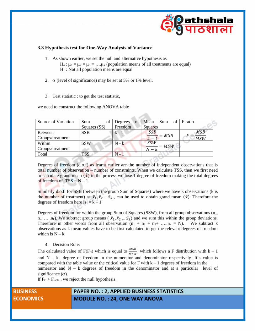
3. Test statistic : to get the test statistic,

we need to construct the following ANOVA table

Source of Variation Sum of

Squares (SS)

Degrees of

Freedom

Mean Sum of

Squares

F ratio

Between

Groups/treatment

SSB k - 1 𝑆𝑆𝐵

𝑘 − 1= 𝑀𝑆𝐵 𝐹 =

𝑀𝑆𝐵

𝑀𝑆𝑊

Within

Groups/treatment

SSW N - k 𝑆𝑆𝑊

𝑁 − 𝑘= 𝑀𝑆𝑊

Total TSS N - 1

Degrees of freedom (d.o.f) as learnt earlier are the number of independent observations that is

total number of observation – number of constraints. When we calculate TSS, then we first need

to calculate grand mean (�̿�) in the process we lose 1 degree of freedom making the total degrees

of freedom of TSS = N – 1.

Similarly d.o.f. for SSB (between the group Sum of Squares) where we have k observations (k is

the number of treatment) as �̅�1, �̅�2 … �̅�𝑘., can be used to obtain grand mean (�̿�). Therefore the

degrees of freedom here is = k – 1

Degrees of freedom for within the group Sum of Squares (SSW), from all group observations (n1,

n2, …..nk). We subtract group means ( �̅�1, �̅�2 … �̅�3) and we sum this within the group deviations.

Therefore in other words from all observation (n1 + n2 + n3+ …..nk = N). We subtract k

observations as k mean values have to be first calculated to get the relevant degrees of freedom

which is N – k.

4. Decision Rule:

The calculated value of F(FC) which is equal to 𝑀𝑆𝐵

𝑀𝑆𝑊 which follows a F distribution with k – 1

and N – k degree of freedom in the numerator and denominator respectively. It’s value is

compared with the table value or the critical value for F with k – 1 degrees of freedom in the

numerator and N – k degrees of freedom in the denominator and at a particular level of

significance ().

If FC > Ftable , we reject the null hypothesis.

____________________________________________________________________________________________________

BUSINESS ECONOMICS



4. Learning One Way ANOVA through Example

4.1 Learning One Way ANOVA

Ques: Given is yield per acre of a variety of crop grown on different plots of land. The plots of

land are grouped according to difference in the treatment that is fertilizer application A,B and C.

The farmer wishes to know that whether there is a significant difference in average crop yield of

the plots due to difference in the fertilizers.

Crop yield per acre due to

Treatment

Samples of Plots

Fertilizer A Fertilizer B Fertilizer C

1 45 24 16

2 40 21 14

3 18 14 38

4 36 18 20

5 19 30 29

Solution:

I Null hypothesis Ho: A = B = C (Average crop yield per plot of land with 3

different types of fertilizer application is equal.

Alternative Hypothesis: Not all average crop yields are same.

II Level of significance: = 5%

III F statistic

Average crop yield per plot after putting fertilizer A

�̅�𝐴 =45 + 40 + 18 + 36 + 19

5= 31.6

Average crop yield per acre after putting fertilizer B

�̅�𝐵 =24 + 21 + 14 + 18 + 30

5= 21.4

Average crop yield per acre after putting fertilizer C

�̅�𝐶 =16 + 14 + 38 + 20 + 29

5= 23.4

Grand mean

�̿� =∑ 𝑥𝑖𝑗

𝑁= 25.47

____________________________________________________________________________________________________

BUSINESS ECONOMICS



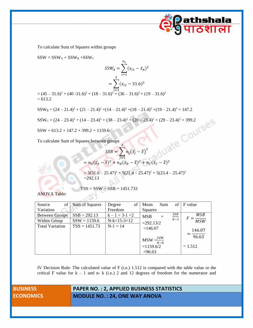
To calculate Sum of Squares within groups

SSW = SSWA + SSWB +SSWC

𝑆𝑆𝑊𝐴 = ∑(𝑥𝑖1 − �̅�𝐴)2

𝑛1

𝑖=1

= ∑(𝑥𝑖1 − 31.6)2

5

𝑖=1

= (45 – 31.6)2 + (40 -31.6)2 + (18 – 31.6)2 + (36 – 31.6)2 + (19 – 31.6)2

= 613.2

SSWB = (24 – 21.4)2 + (21 – 21.4)2 +(14 – 21.4)2 +(18 – 21.4)2 +(19 – 21.4)2 = 147.2

SSWC = (24 – 23.4)2 + (14 – 23.4)2 + (38 – 23.4)2 + (20 – 23.4)2 + (29 – 23.4)2 = 399.2

SSW = 613.2 + 147.2 + 399.2 = 1159.6

To calculate Sum of Squares between groups

𝑆𝑆𝐵 = ∑ 𝑛𝑗(�̅�𝑗 − �̿�)2

3

𝑗=1

= 𝑛𝐴(�̅�𝐴 − �̿�)2 + 𝑛𝐵(�̅�𝐵 − �̿�)2 + 𝑛𝐶(�̅�𝐶 − �̿�)2

= 5(31.6 – 25.47)2 + 5(21.4 – 25.47)2 + 5(23.4 – 25.47)2

=292.13

TSS = SSW + SSB = 1451.733

ANOVA Table:

Source of

Variation

Sum of Squares Degree of

Freedom

Mean Sum of

Squares

F value

Between Groups SSB = 292.13 k – 1 = 3-1 =2 MSB = 𝑆𝑆𝐵

𝑘−1

=292.13/2

=146.07

MSW =𝑆𝑆𝑊

𝑁−𝑘

=1159.6/2

=96.63

𝐹 =𝑀𝑆𝐵

𝑀𝑆𝑊

=146.07

96.63

= 1.512

Within Group SSW = 1159.6 N-k=15-3=12

Total Variation TSS = 1451.73 N-1 = 14

IV Decision Rule: The calculated value of F (i.e.) 1.512 is compared with the table value or the

critical F value for k – 1 and n- k (i.e.) 2 and 12 degrees of freedom for the numerator and

____________________________________________________________________________________________________

BUSINESS ECONOMICS



denominator respectively at 5% level of significance. This value obtained from the F table is 3.89.

If F calculated > Ftable reject Ho which is not the case. Therefore we fail to reject Ho.

Conclusion: We conclude that the impact of all the three fertilizers on average crop yield is

similar.

4.2 Limitations of ANOVA and further tests

Limitations of ANOVA

ANOVA only tells us whether to accept or reject the null hypothesis for equal means. However,

when we reject null hypothesis, ANOVA cannot tell us which of the means are not similar or

equal to the others. It is possible to find this using other test of significance. Two such tests are

widely used which are the Tukey’s method and the Least Significant Difference (LSD) methods.

Case I: When there are equal number of experimental units or samples subject to a treatment.

In the above situation, like our fertilizer example we can use both the Tukey’s and LSD method.

The idea behind both methods is to first calculate a standard value and then compare difference

between all means with this standard value. If the difference in means of some pairs is greater

than this standard value, it would be regarded that the population means of those two groups is

not the same.

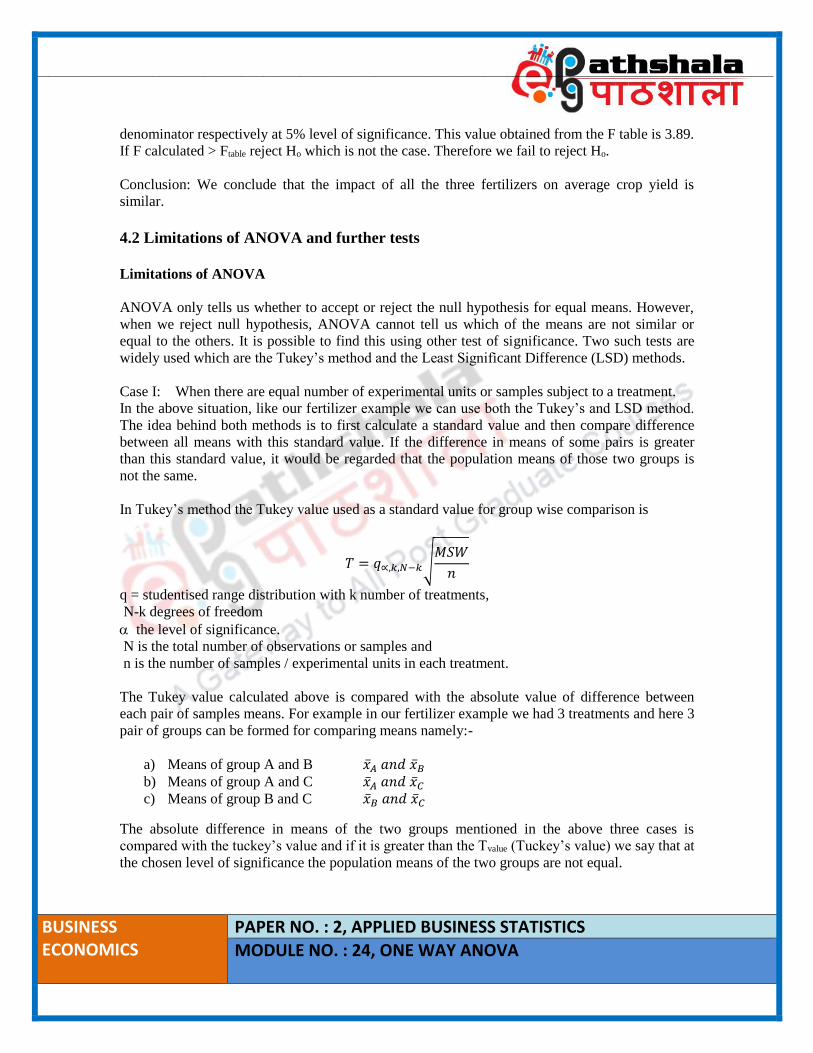
In Tukey’s method the Tukey value used as a standard value for group wise comparison is

𝑇 = 𝑞∝,𝑘,𝑁−𝑘√𝑀𝑆𝑊

𝑛

q = studentised range distribution with k number of treatments,

N-k degrees of freedom

the level of significance.

N is the total number of observations or samples and

n is the number of samples / experimental units in each treatment.

The Tukey value calculated above is compared with the absolute value of difference between

each pair of samples means. For example in our fertilizer example we had 3 treatments and here 3

pair of groups can be formed for comparing means namely:-

a) Means of group A and B �̅�𝐴 𝑎𝑛𝑑 �̅�𝐵 b) Means of group A and C �̅�𝐴 𝑎𝑛𝑑 �̅�𝐶 c) Means of group B and C �̅�𝐵 𝑎𝑛𝑑 �̅�𝐶

The absolute difference in means of the two groups mentioned in the above three cases is

compared with the tuckey’s value and if it is greater than the Tvalue (Tuckey’s value) we say that at

the chosen level of significance the population means of the two groups are not equal.

____________________________________________________________________________________________________

BUSINESS ECONOMICS



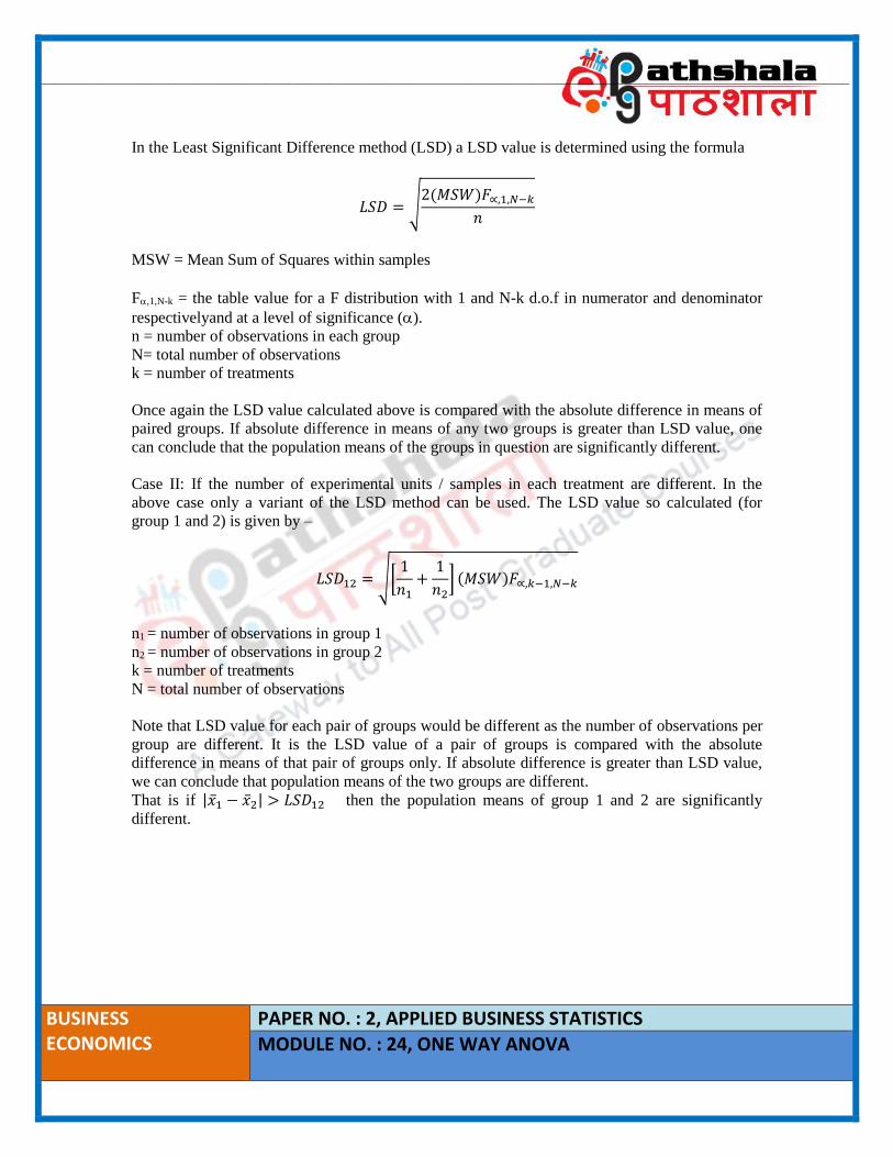
In the Least Significant Difference method (LSD) a LSD value is determined using the formula

𝐿𝑆𝐷 = √2(𝑀𝑆𝑊)𝐹∝,1,𝑁−𝑘

𝑛

MSW = Mean Sum of Squares within samples

F,1,N-k = the table value for a F distribution with 1 and N-k d.o.f in numerator and denominator

respectivelyand at a level of significance ().

n = number of observations in each group

N= total number of observations

k = number of treatments

Once again the LSD value calculated above is compared with the absolute difference in means of

paired groups. If absolute difference in means of any two groups is greater than LSD value, one

can conclude that the population means of the groups in question are significantly different.

Case II: If the number of experimental units / samples in each treatment are different. In the

above case only a variant of the LSD method can be used. The LSD value so calculated (for

group 1 and 2) is given by –

𝐿𝑆𝐷12 = √[1

𝑛1+

1

𝑛2] (𝑀𝑆𝑊)𝐹∝,𝑘−1,𝑁−𝑘

n1 = number of observations in group 1

n2 = number of observations in group 2

k = number of treatments

N = total number of observations

Note that LSD value for each pair of groups would be different as the number of observations per

group are different. It is the LSD value of a pair of groups is compared with the absolute

difference in means of that pair of groups only. If absolute difference is greater than LSD value,

we can conclude that population means of the two groups are different.

That is if |�̅�1 − �̅�2| > 𝐿𝑆𝐷12 then the population means of group 1 and 2 are significantly

different.

____________________________________________________________________________________________________

BUSINESS ECONOMICS



5. Summary

One Way ANOVA helps to study whether there is difference in means of more than two

samples

To study whether population means are different or not, this method studies the various

sources of variation namely within the group and between groups.

The test statistic used here is the F ratio which is the ratio of Between the Group Mean Sum

of Squares (MSB) and Within the Group Mean Sum of Squares (MSW).

The Calculated value of F is compared with critical (table value) with relevant degrees of

freedom in the numerator and denominator at a particular level of significance. If calculated F

is greater than Critical F, we reject the null hypothesis of no difference between means.

Once we conclude that there is significant difference between sample means, Tuckey’s test

and Least Significant Difference (LSD) methods help us to identify which sample means are

not equal.

BSc Chemistry - e-PG Pathshala

Documents

Transcript of BSc Chemistry - e-PG Pathshala