arX

iv:h

ep-p

h/99

1248

8v1

23

Dec

199

9

Preprint typeset in JHEP style. - PAPER VERSION Bicocca–FT–99–32

CERN–TH/99–396

hep-ph/9912488

December 1999

Resummation of thrust distributions in DIS∗

Vito Antonelli, Mrinal Dasgupta

Dipartimento di Fisica, Universita di Milano Bicocca and INFN, Sezione di

Milano, Italy

Gavin P. Salam

CERN, TH Division, 1211 Geneva 23, Switzerland

Abstract: We calculate the resummed distributions for the thrust in DIS in the

limit T → 1. Two variants of the thrust are considered: that normalised to Q/2, and

that normalised to the energy in the current hemisphere. The results expanded to

second order are compared to predictions from the Monte Carlo programs DISENT

and DISASTER++. A prescription is given for matching the resummed expressions

with the full fixed order calculation.

Keywords: QCD, NLO Computations, Jets, Deep Inelastic Scattering.

∗Research supported in part by MURST, Italy and by the EU Fourth Framework Programme

‘Training and Mobility of Researchers’, Network ‘Quantum Chromodynamics and the Deep Struc-

ture of Elementary Particles’, contract FMRX-CT98-0194 (DG 12-MIHT).

Contents

1. Introduction 1

2. Thrust definitions and kinematics 3

2.1 Thrust normalised to Q/2, TQ 4

2.2 Thrust normalised to E, TE 5

3. Resummation 5

3.1 Resummation of τQ 6

3.2 Resummation of τE 10

4. The final result 12

4.1 Comparison with NLO computations 13

4.2 Matching 14

5. Conclusions 18

A. Leading order calculations 19

B. Inverse Mellin transforms 20

C. Two-loop radiator integrals 21

1. Introduction

For some time now it has been standard practice in e+e− reactions to compare event-

shape distributions with resummed perturbative predictions (see for instance [1]).

The resummation is necessary because in the two-jet limit (small values of the shape

variable) the presence of large logarithms spoils the convergence of the fixed-order

calculations. Such resummed analyses have led to valuable information about the

strong coupling constant and also about non-perturbative effects [2].

At HERA, similar studies of DIS event-shape distributions are being carried

out by both collaborations [3, 4], but as yet no perturbative resummed calculations

exist for comparison between data and theory. Here we present the results of such a

calculation.

So far resummed predictions for processes involving initial state hadrons exist

for observables such as DIS and Drell-Yan cross-sections in the semi-inclusive limits

1

where x for DIS and τ for Drell-Yan are close to one [5–7]. In addition there are

predictions for jet-multiplicities in DIS [8] and the W transverse momentum in Drell-

Yan production [9] which entail somewhat similar considerations to those that are

encountered here.

In DIS, event shapes are defined in the current hemisphere of the Breit frame

to reduce contamination from remnant fragmentation, which is beyond perturbative

control [10]. The distribution of partons in the current hemisphere is analogous to

that in a single hemisphere in e+e−, enabling us to adopt the usual e+e− methods

for the resummation. But it turns out that event-shape variables also depend on

emissions in the remnant hemisphere (typically through recoil effects) — a proper

resummed treatment of the space-like branching of the incoming parton is therefore

required.

The fact that only one, predefined, hemisphere is used in DIS event shapes leads

to a number of subtleties compared to e+e− event shapes. Event shapes measure

properties of the energy-momentum flow in the current hemisphere. They are always

dimensionless, so it is necessary to normalise this measure of energy-momentum flow.

Two choices are possible: a normalisation to Q/2, or to E, the energy in the current

hemisphere (whereas in e+e− the total energy E is equal to Q). Furthermore, one

often requires the choice of an axis along which to project the momentum flow (for

example for the thrust, the broadening). In e+e− there is one logical choice of axis,

namely the thrust axis (that which maximises the thrust). In DIS, two axes arise

naturally: the photon axis and the thrust axis (which is given by the direction of the

sum of all momenta in the current hemisphere).

In this article we shall consider two variants of the thrust. Both are measured

with respect to the photon axis: one, TQ, is normalised to Q/2 and the other, TE ,

is normalised to E. In the limit of a 1+1 jet event both tend to T = 1. Since we

are particularly interested in this limit, it will be convenient to define τ = 1−T and

consider the limit of small τ . While we are generally interested in the differential

distribution 1σ

dσdτ

, it will turn out to be more convenient to look at the integrated

event-shape cross section

Σ(τ) =

∫ τ

0

dτ ′dσ

dτ ′, (1.1)

from which the distribution can be straightforwardly obtained by differentiation.

For small τ one finds that the shape cross-section contains terms αns lnm τ, m ≤

2n coming from multiple soft and collinear radiation. The ln τ factors compensate

the smallness of αs, hence the need arises for resummation, which leads to a result

schematically of the form Σ(τ) ∼ exp(−G12αs ln2 τ + . . . ), with G12 some number

which will be calculated. From the point of view of classifying the terms that we shall

calculate, it turns out to be most convenient to consider lnΣ. This contains terms

αns

lnm τ with m ≤ n+1. Terms with m = n+1 are referred to as leading logarithmic

2

(LL), while those with m = n are known as next-to-leading logarithmic (NLL). We

shall resum both these sets of terms, and neglect as subleading the remaining terms,

m < n.

A word of caution is needed about τE , and in general about all event-shape

measures which are normalised to the energy in the current hemisphere, E. At O (αs)

there are configurations in which the current hemisphere is empty. At higher orders

it can be filled by soft-gluon radiation from the partons in the remnant hemisphere.

If the event-shape is normalised to E then it can take on finite (significantly different

from 0 and/or 1) values due to the presence of soft-radiation; in other words it will

be infrared unsafe starting from O (α2s). This has been known for some time. The

standard experimental practice is to exclude events in which the energy in the current

hemisphere is too low. For example, H1 set the threshold E > Elim = Q/10 [3].

Though formally this eliminates any infrared unsafety, one is still left with potentially

large logs αs(αs lnQ/2Elim)n. Thus we recommend that Elim be chosen somewhat

larger, say Elim = Q/4. Though this will slightly reduce the statistics, it ought to

improve the convergence of the perturbation series.

The structure of this article is as follows. In section 2 we discuss the kinematics

and define the thrust measures which will be studied. In section 3 we perform the

resummations. Section 4 gives the expressions to be used for the practical calculation

of resummed distributions. The results are expanded to second order and compared

to the predictions from the fixed order Monte Carlo programs DISASTER++ [11]

and DISENT [12]. This enables us to cast some light on the differences between

DISASTER++ and DISENT, observed in [13]. Finally a matching prescription is

proposed for combining the resummed and fixed order predictions. This is followed

by the conclusions.

The appendices provide details about the leading order calculation of the thrust

(appendix A), the techniques used for the inverse Mellin transforms (appendix B)

and the integrations needed for a result correct to NLL (appendix C).

2. Thrust definitions and kinematics

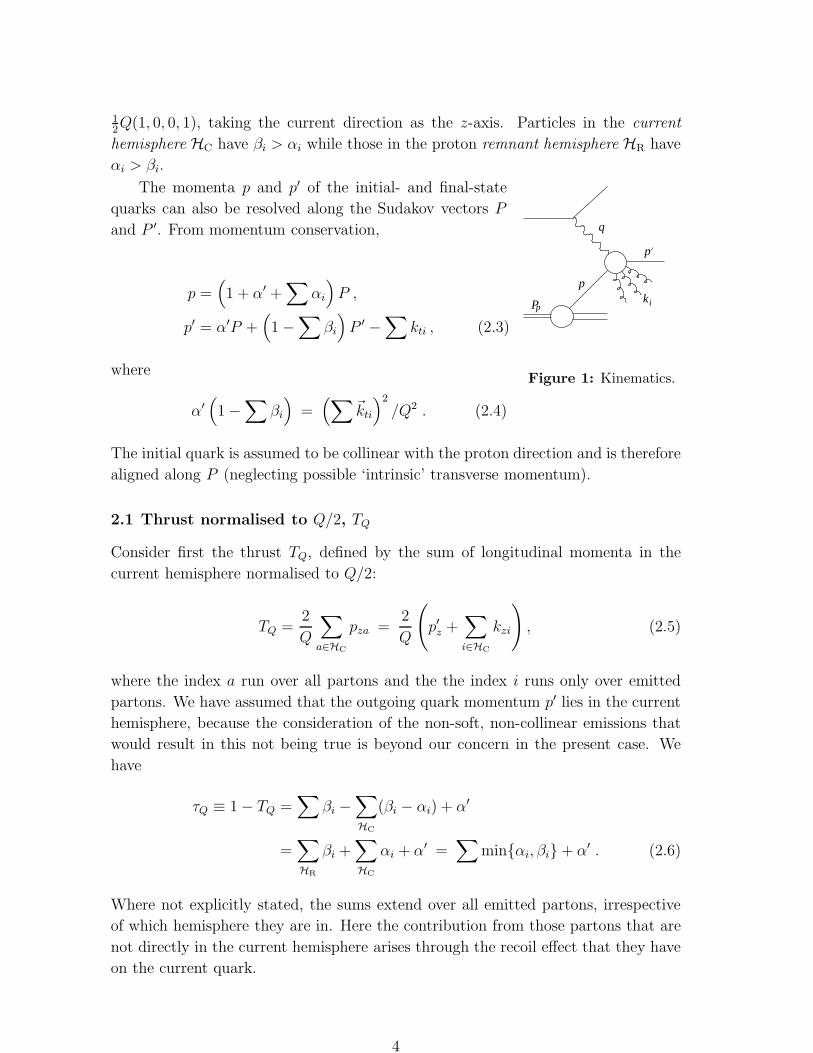
It is convenient to write the momenta ki of radiated partons (gluons and/or

quark-antiquark pairs) in terms of Sudakov (light-cone) variables as (Fig. 1)

ki = αiP + βiP′ + kti , αiβi = ~k2

ti/Q2 (2.1)

where P and P ′ are light-like vectors along the incoming parton and current direc-

tions, respectively, in the Breit frame of reference:

P = xPp , P′ = xPp + q , 2(P · P ′) = −q2 ≡ Q2 (2.2)

where Pp is the incoming proton momentum and x = Q2/2(Pp · q) is the Bjorken

variable. Thus in the Breit frame we can write P = 12Q(1, 0, 0,−1) and P ′ =

3

12Q(1, 0, 0, 1), taking the current direction as the z-axis. Particles in the current

hemisphere HC have βi > αi while those in the proton remnant hemisphere HR have

αi > βi.

The momenta p and p′ of the initial- and final-state

P

p

q

pki

p

Figure 1: Kinematics.

quarks can also be resolved along the Sudakov vectors P

and P ′. From momentum conservation,

p =(1 + α′ +

∑αi

)P ,

p′ = α′P +(1 −

∑βi

)P ′ −

∑kti , (2.3)

where

α′

(1 −

∑βi

)=(∑

~kti

)2

/Q2 . (2.4)

The initial quark is assumed to be collinear with the proton direction and is therefore

aligned along P (neglecting possible ‘intrinsic’ transverse momentum).

2.1 Thrust normalised to Q/2, TQ

Consider first the thrust TQ, defined by the sum of longitudinal momenta in the

current hemisphere normalised to Q/2:

TQ =2

Q

∑

a∈HC

pza =2

Q

(p′z +

∑

i∈HC

kzi

), (2.5)

where the index a run over all partons and the the index i runs only over emitted

partons. We have assumed that the outgoing quark momentum p′ lies in the current

hemisphere, because the consideration of the non-soft, non-collinear emissions that

would result in this not being true is beyond our concern in the present case. We

have

τQ ≡ 1 − TQ =∑

βi −∑

HC

(βi − αi) + α′

=∑

HR

βi +∑

HC

αi + α′ =∑

min{αi, βi} + α′ . (2.6)

Where not explicitly stated, the sums extend over all emitted partons, irrespective

of which hemisphere they are in. Here the contribution from those partons that are

not directly in the current hemisphere arises through the recoil effect that they have

on the current quark.

4

2.2 Thrust normalised to E, TE

Another way to define the current jet thrust is to normalise it to the total energy in

the current hemisphere, instead of Q/2. This gives

TE = TQ/(1 − ε) , (2.7)

where

ε ≡ 1 −2

Q

∑

a∈HC

Ea . (2.8)

The quantity ε, called the energy deficit in the current hemisphere, is itself an inter-

esting shape variable [14]. It is given by

ε =∑

βi −∑

HC

(βi + αi) − α′ =∑

HR

βi −∑

HC

αi − α′ . (2.9)

Hence, we have,

τE = 1 − TE =2

1 −∑

HRβi +

∑HC

αi + α′

(∑

HC

αi + α′

). (2.10)

3. Resummation

We shall consider a reduced integrated cross section, where by reduced we mean

that it will be the contribution to F2 (rather than to dσ/dxdQ2) which comes from

configurations with 1 − T < τ . There will be no need to consider contributions to

FL since they are suppressed by powers of τ for small τ .

We write the following expression for the (reduced) cross section for the emission

of m gluons in the remnant hemisphere and n in the current hemisphere, where all

the gluons have kt ≪ Q,

e2qqN(Q20) ·

1

m!

m∏

i

∫ Q2

Q20

dk2ti

k2ti

αs(k2ti)CF

2πρR,i ·

1

n!

n∏

j

∫ Q2dk2

tj

k2tj

αs(k2tj)CF

2πρC,j . (3.1)

with

ρR,i =

∫zN

i dzi1 + z2

i

1 − ziΘ(Qαi − kti), (3.2a)

ρC,j =

∫dβj

βj

(1 + (1 − βj)

2)Θ(Qβj − ktj). (3.2b)

N is the moment variable (conjugate to Bjorken-x) and

αi =1 − zi

z1 . . . zi. (3.3)

5

We have introduced a factorisation scale Q20, and accordingly in HR consider only

emissions above that scale. Q20 is chosen so as to be much smaller than any other

scale in the problem.

For the event shapes considered here, the independent gluon emission pattern

written above is enough to reproduce the behaviour of the full QCD matrix elements

up to the required (NLL) accuracy, with the following restrictions: αs must be eval-

uated to two loops in the CMW (or Physical) scheme [7,15]; we must also put in the

virtual corrections and take into account all possible branchings of the incoming leg,

not just the emission of gluons from a quark; but these can both be done trivially

later on. It is not necessary to take into account the splitting of emitted partons,

other than what is already implicitly included through the running of the coupling.

The fundamental difference between the expression given above and the corre-

sponding one for e+e− comes from the presence of the quark distribution. Hard

collinear emissions change the momentum fraction of the incoming parton, and this

must be accounted for, through a (multiple) convolution of some function (to be

determined) with the parton distributions. We take moments (N) with respect to x

in order convert that convolution into a product. These moments enter only for the

emissions in HR — emissions in HC are essentially identical to those in a hemisphere

of e+e−.

The use of moments does not however remove all difficulties. In particular in

eq. (3.3) we are still left with a product of zi’s. This matters both in the Θ function

in eq. (3.2a) and in the contribution to the thrust, which for say τQ will be βi =

k2ti/(Q

2αi) (cf. eq. (2.6)). The solution relies on the fact that the gluons which

contribute to the thrust are either the gluon with the highest transverse momentum

or soft gluons. Considering the gluons as ordered in transverse momentum, the

gluon with highest transverse momentum is number 1 and α1 = (1−z1)/z1. One can

equally well consider the gluons to be ordered in angle, and if gluon m has the highest

transverse momentum, then gluons with i < m must have 1 − zi ≪ 1 and one can

write αm ≃ (1 − zm)/zm. For soft gluons we can approximate the splitting function

by 2/(1 − zi), and then replace (1 − zi)/(z1 . . . zi−1) ⇒ (1 − ζi). The integration

measure remains 2dζi/(1− ζi), and αi just becomes (1− ζi)/ζi. So we can in general

just replace αi by (1− zi)/zi (where zi should sometimes be understood to mean ζi).

3.1 Resummation of τQ

To write a resummed expression we take the Mellin transform of our Θ function for

τQ:

Θ

(τ −

∑

HR

βj −∑

HC

αi − α′

)=

∫dν

2πiνeτν

(∏

HR

e−νβi

)(∏

HC

e−ναi

)e−να′

. (3.4)

This almost factorises the expression for the Θ function into pieces which each depend

on a single emission. There remains the less trivial term e−να′

: from (2.4) we know

6

that α′ is approximately (using 1 −∑β ≃ 1) the squared vector sum of emitted

transverse momenta. For now it is actually sufficient to consider the sum of squared

momenta. For soft and collinear gluons k2ti/Q

2 = αiβi is negligible compared to

min(αi, βi). Only for collinear but hard gluons is k2ti/Q

2 comparable to min(αi, βi)

because one of the αi, βi is O (1). In the current hemisphere, since βi < 1, the

contribution from the k2t /Q

2 can be neglected: the region where it is comparable to

αi is single-logarithmic and its inclusion modifies τ by a numerical factor, i.e. changes

αs ln τ to say αs ln 2τ , a difference which is NNLL and so negligible. The difference

is similarly NNLL in the remnant hemisphere, however the fact that αi can be much

greater than 1 (as large as 1/x), and hence k2ti/Q

2 ≫ βi, means that one should at

least keep track of it. Therefore in the remnant hemisphere contribution we retain

a contribution to τ of the form k2t /Q

2 (keeping track of it more accurately would

involve using the squared vector sum — but for τQ the error is down by one more

logarithm). Thus we replace

(∏

HR

e−νβi

)(∏

HC

e−ναi

)e−να′

⇒

(∏

HR

e−ν(βi+k2ti/Q2)

)(∏

HC

e−ναi

). (3.5)

We then sum over m and n in (3.1) to give us the following exponentiated form

for the integrated thrust distribution

ΣN(τ) = e2qqN (Q2)

∫dν

2πiνeτν e−RR(ν)−RC(ν) . (3.6)

The current hemisphere radiator, RC is

RC(ν) = −

∫dk2

t

k2t

αs(k2t )CF

2π

∫ 1

0

dβ1 + (1 − β)2

βΘ(Qβ − kt)

(e−να − 1

), (3.7)

where the −1 accounts for virtual corrections (as in [16]). The remnant hemisphere

radiator is a little trickier. The attentive reader will have noticed that eq. (3.1)

has a leading factor of qN (Q20), whereas eq. (3.6) has qN(Q2). Thus RR(ν) should

contain a (ν-independent) piece to take into account the change in scale of the quark

distribution,

lnqN(Q2)

qN(Q20)

=

∫ Q2

Q20

dk2t

k2t

αs(k2t )

2πγqq(N), (3.8)

(where γqq is the standard quark anomalous dimension) as well as the part arising

from the sum over m in eq. (3.1). For now we are still working in a framework

involving only gluon emission from a quark, hence the use of only the γqq part of the

anomalous dimension matrix to change the scale of the quark distribution.

7

Therefore we have

RR(ν) = −

∫ Q2

Q20

dk2t

k2t

αs(k2t )CF

2π

(∫ 1

0

dz1 + z2

1 − zΘ(Qα− kt)

(zNe−ν(β+k2

t /Q2) − 1)

−γqq(N)

CF

), (3.9)

where as before we have introduced a term −1 to account for virtual corrections.

Next, we replace α = (1 − z)/z. In the Θ function we can neglect the z in the

denominator (the Θ function is relevant only for small 1 − z). So we obtain

RR(ν) = −

∫ Q2

Q20

dk2t

k2t

αs(k2t )CF

2π

(∫ 1

0

dz1 + z2

1 − zΘ(1 − z − kt/Q)

(zNe

−νk2

t(1−z)Q2 − 1

)

−γqq(N)

CF

). (3.10)

We note that in the limit of small z the combination (β+k2t /Q

2) just reduces to k2t /Q

2,

i.e. a limit on τ is just equivalent to a limit on the emitted transverse momentum.

Then we write

γqq(N) = CF

∫ 1

0

dz1 + z2

1 − z(zN − 1)Θ(1 − z − kt/Q) + O

(kt

Q

), (3.11)

to obtain

RR(ν) = −

∫ Q2

dk2t

k2t

αs(k2t )CF

2π

∫ 1

0

dz zN 1 + z2

1 − zΘ(1 − z − kt/Q)

(e−

νk2t

(1−z)Q2 − 1

).

(3.12)

The result no longer depends on our original choice of factorisation scale, Q20, and

thus we drop the lower limit on the kt integral. Our next step is to make the

approximation, valid to our accuracy [16],

(e−

νk2t

Q2(1−z) − 1

)≃ −Θ

(ν −

Q2(1 − z)

k2t

)(3.13)

with ν = νeγe . The kt integral can then be divided into two pieces (according to

whether the limit on 1 − z in the Θ-function of (3.13) is above or below 1)

RR(ν) =

∫ Q2

Q2ν−1

dk2t

k2t

αs(k2t )CF

2π

∫ 1−kt/Q

0

dz zN 1 + z2

1 − z

+

∫ Q2ν−1

Q2ν−2

dk2t

k2t

αs(k2t )CF

2π

∫ 1−kt/Q

1−νk2t /Q2

dz2

1 − z, (3.14)

8

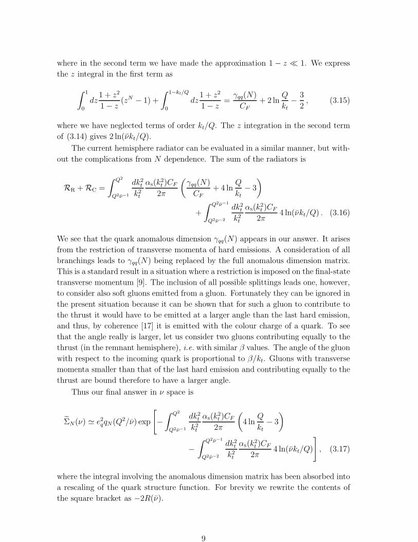
where in the second term we have made the approximation 1 − z ≪ 1. We express

the z integral in the first term as

∫ 1

0

dz1 + z2

1 − z(zN − 1) +

∫ 1−kt/Q

0

dz1 + z2

1 − z=γqq(N)

CF+ 2 ln

Q

kt−

3

2, (3.15)

where we have neglected terms of order kt/Q. The z integration in the second term

of (3.14) gives 2 ln(νkt/Q).

The current hemisphere radiator can be evaluated in a similar manner, but with-

out the complications from N dependence. The sum of the radiators is

RR + RC =

∫ Q2

Q2ν−1

dk2t

k2t

αs(k2t )CF

2π

(γqq(N)

CF+ 4 ln

Q

kt− 3

)

+

∫ Q2ν−1

Q2ν−2

dk2t

k2t

αs(k2t )CF

2π4 ln(νkt/Q) . (3.16)

We see that the quark anomalous dimension γqq(N) appears in our answer. It arises

from the restriction of transverse momenta of hard emissions. A consideration of all

branchings leads to γqq(N) being replaced by the full anomalous dimension matrix.

This is a standard result in a situation where a restriction is imposed on the final-state

transverse momentum [9]. The inclusion of all possible splittings leads one, however,

to consider also soft gluons emitted from a gluon. Fortunately they can be ignored in

the present situation because it can be shown that for such a gluon to contribute to

the thrust it would have to be emitted at a larger angle than the last hard emission,

and thus, by coherence [17] it is emitted with the colour charge of a quark. To see

that the angle really is larger, let us consider two gluons contributing equally to the

thrust (in the remnant hemisphere), i.e. with similar β values. The angle of the gluon

with respect to the incoming quark is proportional to β/kt. Gluons with transverse

momenta smaller than that of the last hard emission and contributing equally to the

thrust are bound therefore to have a larger angle.

Thus our final answer in ν space is

ΣN(ν) ≃ e2qqN (Q2/ν) exp

[−

∫ Q2

Q2ν−1

dk2t

k2t

αs(k2t )CF

2π

(4 ln

Q

kt− 3

)

−

∫ Q2ν−1

Q2ν−2

dk2t

k2t

αs(k2t )CF

2π4 ln(νkt/Q)

], (3.17)

where the integral involving the anomalous dimension matrix has been absorbed into

a rescaling of the quark structure function. For brevity we rewrite the contents of

the square bracket as −2R(ν).

9

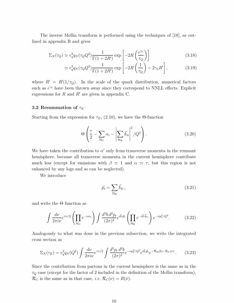
The inverse Mellin transform is performed using the techniques of [18], as out-

lined in appendix B and gives

ΣN (τQ) ≃ e2qqN (τQQ2)

1

Γ(1 + 2R′)exp

[−2R

(eγe

τQ

)](3.18)

≃ e2qqN (τQQ2)

1

Γ(1 + 2R′)exp

[−2R

(1

τQ

)− 2γeR

′

], (3.19)

where R′ = R′(1/τQ). In the scale of the quark distribution, numerical factors

such as eγe have been thrown away since they correspond to NNLL effects. Explicit

expressions for R and R′ are given in appendix C.

3.2 Resummation of τE

Starting from the expression for τE , (2.10), we have the Θ-function

Θ

τ2−∑

HC

αi −

∣∣∣∣∣∑

HR

~kti

∣∣∣∣∣

2

/Q2

. (3.20)

We have taken the contribution to α′ only from transverse momenta in the remnant

hemisphere, because all transverse momenta in the current hemisphere contribute

much less (except for emissions with β ≃ 1 and α ≃ τ , but this region is not

enhanced by any logs and so can be neglected).

We introduce

~pt =∑

HR

~kti , (3.21)

and write the Θ function as

∫dν

2πiνeτν/2

(∏

HC

e−ναi

)∫d2b d2pt

(2π)2ei~b.~pt

(∏

HR

e−i~b.~kti

)e−νp2

t /Q2

. (3.22)

Analogously to what was done in the previous subsection, we write the integrated

cross section as

ΣN (τE) = e2qqN (Q2)

∫dν

2πiνeτν/2

∫d2pt d

2b

(2π)2e−νp2

t /Q2

ei~b.~pte−RR(b)−RC(ν) . (3.23)

Since the contribution from partons in the current hemisphere is the same as in the

τQ case (except for the factor of 2 included in the definition of the Mellin transform),

RC is the same as in that case, i.e. RC(ν) = R(ν).

10

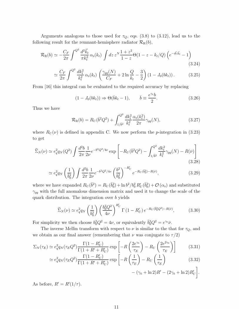
Arguments analogous to those used for τQ, eqs. (3.8) to (3.12), lead us to the

following result for the remnant-hemisphere radiator RR(b),

RR(b) ≃ −CF

2π

∫ Q2

d2~kt

πk2t

αs(kt)

∫dz zN 1 + z2

1 − zΘ(1 − z − kt/Q)

(e−i~b.~kt − 1

)

(3.24)

≃CF

2π

∫ Q2

dk2t

k2t

αs(kt)

(γqq(N)

CF+ 2 ln

Q

kt−

3

2

)(1 − J0(bkt)) . (3.25)

From [16] this integral can be evaluated to the required accuracy by replacing

(1 − J0(bkt)) ⇒ Θ(bkt − 1), b ≡eγeb

2. (3.26)

Thus we have

RR(b) = RU (b2Q2) +

∫ Q2

1/b2

dk2t

k2t

αs(k2t )

2πγqq(N), (3.27)

where RU(ν) is defined in appendix C. We now perform the p-integration in (3.23)

to get

ΣN(ν) ≃ e2qqN (Q2)

∫d2b

2π

1

2νe−b2Q2/4ν exp

[−RU(b2Q2) −

∫ Q2

1/b2

dk2t

k2t

γqq(N) − R(ν)

]

(3.28)

≃ e2qqN

(1

b20

)∫d2b

2π

1

2νe−b2Q2/4ν

(b2

b20

)−R′

U

e−RU (b20)−R(ν), (3.29)

where we have expanded RU(b2) = RU (b20)+ ln b2/b20R′U (b20)+O (αs) and substituted

γqq with the full anomalous dimension matrix and used it to change the scale of the

quark distribution. The integration over b yields

ΣN (ν) ≃ e2qqN

(1

b20

)(b20Q

2

4ν

)R′

U

Γ (1 −R′

U) e−RU (b20Q2)−R(ν), (3.30)

For simplicity we then choose b20Q2 = 4ν, or equivalently b20Q

2 = eγe ν.

The inverse Mellin transform with respect to ν is similar to the that for τQ, and

we obtain as our final answer (remembering that ν was conjugate to τ/2)

ΣN (τE) ≃ e2qqN (τEQ2)

Γ(1 −R′U)

Γ(1 +R′ +R′U)

exp

[−R

(2eγe

τE

)− RU

(2e2γe

τE

)](3.31)

≃ e2qqN (τEQ2)

Γ(1 −R′U)

Γ(1 +R′ +R′U)

exp

[−R

(1

τE

)− RU

(1

τE

)(3.32)

− (γe + ln 2)R′ − (2γe + ln 2)R′

U

].

As before, R′ = R′(1/τ).

11

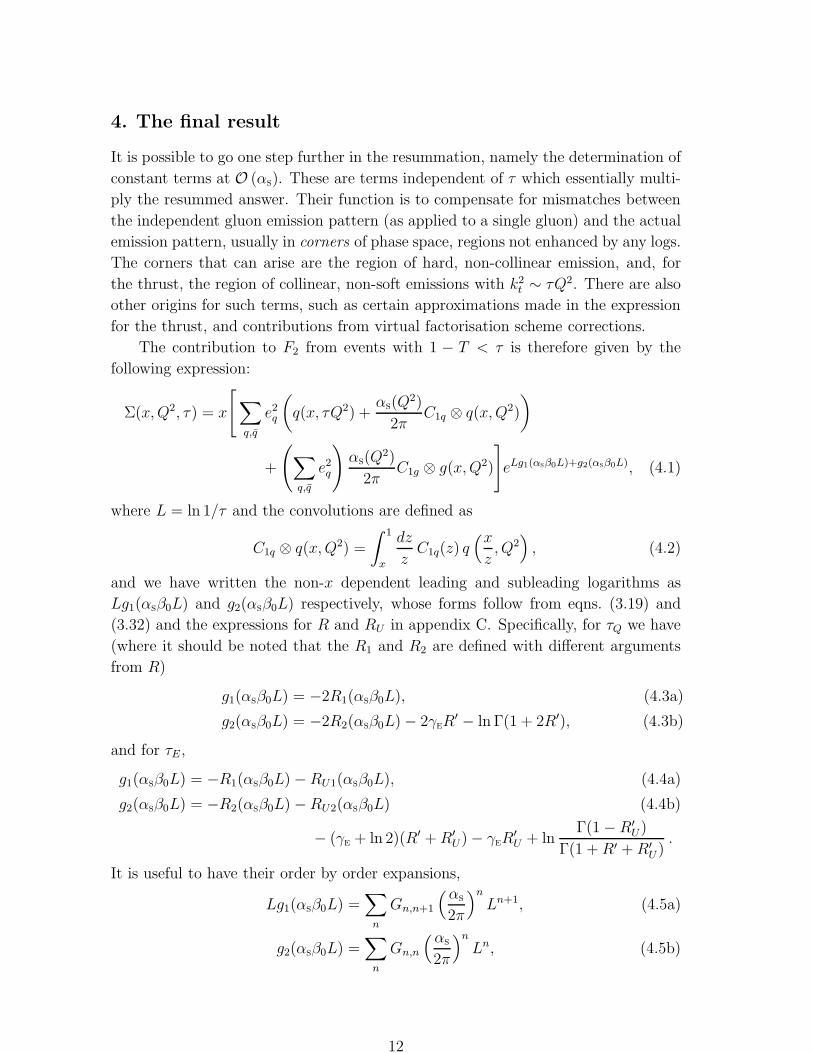
4. The final result

It is possible to go one step further in the resummation, namely the determination of

constant terms at O (αs). These are terms independent of τ which essentially multi-

ply the resummed answer. Their function is to compensate for mismatches between

the independent gluon emission pattern (as applied to a single gluon) and the actual

emission pattern, usually in corners of phase space, regions not enhanced by any logs.

The corners that can arise are the region of hard, non-collinear emission, and, for

the thrust, the region of collinear, non-soft emissions with k2t ∼ τQ2. There are also

other origins for such terms, such as certain approximations made in the expression

for the thrust, and contributions from virtual factorisation scheme corrections.

The contribution to F2 from events with 1 − T < τ is therefore given by the

following expression:

Σ(x,Q2, τ) = x

[∑

q,q

e2q

(q(x, τQ2) +

αs(Q2)

2πC1q ⊗ q(x,Q2)

)

+

(∑

q,q

e2q

)αs(Q

2)

2πC1g ⊗ g(x,Q2)

]eLg1(αsβ0L)+g2(αsβ0L), (4.1)

where L = ln 1/τ and the convolutions are defined as

C1q ⊗ q(x,Q2) =

∫ 1

x

dz

zC1q(z) q

(xz,Q2

), (4.2)

and we have written the non-x dependent leading and subleading logarithms as

Lg1(αsβ0L) and g2(αsβ0L) respectively, whose forms follow from eqns. (3.19) and

(3.32) and the expressions for R and RU in appendix C. Specifically, for τQ we have

(where it should be noted that the R1 and R2 are defined with different arguments

from R)

g1(αsβ0L) = −2R1(αsβ0L), (4.3a)

g2(αsβ0L) = −2R2(αsβ0L) − 2γeR′ − ln Γ(1 + 2R′), (4.3b)

and for τE ,

g1(αsβ0L) = −R1(αsβ0L) −RU1(αsβ0L), (4.4a)

g2(αsβ0L) = −R2(αsβ0L) −RU2(αsβ0L) (4.4b)

− (γe + ln 2)(R′ +R′

U) − γeR′

U + lnΓ(1 − R′

U)

Γ(1 +R′ +R′U ).

It is useful to have their order by order expansions,

Lg1(αsβ0L) =∑

n

Gn,n+1

(αs

2π

)n

Ln+1, (4.5a)

g2(αsβ0L) =∑

n

Gn,n

(αs

2π

)n

Ln, (4.5b)

12

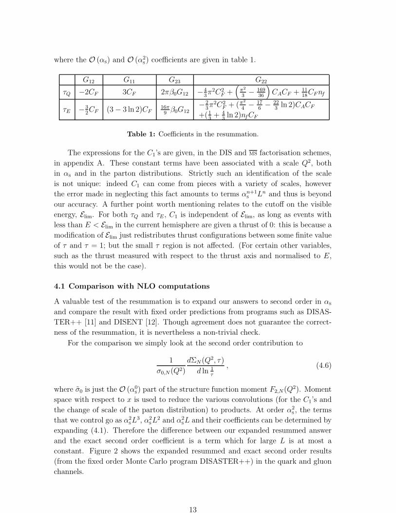
where the O (αs) and O (α2s) coefficients are given in table 1.

G12 G11 G23 G22

τQ −2CF 3CF 2πβ0G12 −43π2C2

F +(

π2

3− 169

36

)CACF + 11

18CFnf

τE −32CF (3 − 3 ln 2)CF

16π9β0G12

−23π2C2

F + (π2

4− 17

6− 22

3ln 2)CACF

+(13

+ 43ln 2)nfCF

Table 1: Coefficients in the resummation.

The expressions for the C1’s are given, in the DIS and MS factorisation schemes,

in appendix A. These constant terms have been associated with a scale Q2, both

in αs and in the parton distributions. Strictly such an identification of the scale

is not unique: indeed C1 can come from pieces with a variety of scales, however

the error made in neglecting this fact amounts to terms αn+1s

Ln and thus is beyond

our accuracy. A further point worth mentioning relates to the cutoff on the visible

energy, Elim. For both τQ and τE , C1 is independent of Elim, as long as events with

less than E < Elim in the current hemisphere are given a thrust of 0: this is because a

modification of Elim just redistributes thrust configurations between some finite value

of τ and τ = 1; but the small τ region is not affected. (For certain other variables,

such as the thrust measured with respect to the thrust axis and normalised to E,

this would not be the case).

4.1 Comparison with NLO computations

A valuable test of the resummation is to expand our answers to second order in αs

and compare the result with fixed order predictions from programs such as DISAS-

TER++ [11] and DISENT [12]. Though agreement does not guarantee the correct-

ness of the resummation, it is nevertheless a non-trivial check.

For the comparison we simply look at the second order contribution to

1

σ0,N (Q2)

dΣN (Q2, τ)

d ln 1τ

, (4.6)

where σ0 is just the O (α0s) part of the structure function moment F2,N(Q2). Moment

space with respect to x is used to reduce the various convolutions (for the C1’s and

the change of scale of the parton distribution) to products. At order α2s , the terms

that we control go as α2sL3, α2

sL2 and α2

sL and their coefficients can be determined by

expanding (4.1). Therefore the difference between our expanded resummed answer

and the exact second order coefficient is a term which for large L is at most a

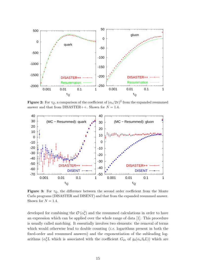
constant. Figure 2 shows the expanded resummed and exact second order results

(from the fixed order Monte Carlo program DISASTER++) in the quark and gluon

channels.

13

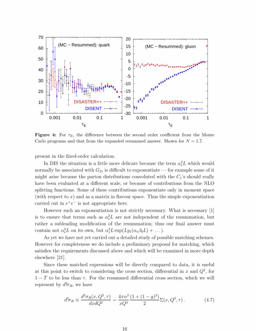
The shape of the resummed and exact results are clearly similar and the difference

between them does seem to tend to a constant at small τ . This is visible more clearly

in figure 3 which shows the difference between the two results. Also shown is the

difference between the current version (0.1) of DISENT and the resummed answer.

In the gluon channel the difference is clearly inconsistent with a constant: it seems

to go as α2sL2. In the quark channel there is also evidence of similar problems, with

a significance of a few (between 3 and 5) standard deviations. Results are shown for

τE in figure 4, where the same pattern of successes and problems is seen.

The origin of the discrepancy in DISENT has yet to be elucidated. However it

has been possible to identify that the disagreement lies in pieces proportional to C2F

(quark channel) and CATR (gluon channel). Furthermore the fact that, in the gluon

channel, the disagreement is at the level of a α2sL2 term in the distribution (α2

sL3

in the integrated distribution) suggests that the problem lies with a term involving

one soft and two collinear divergences. In the gluon channel there should be no

term α2sL2 with colour factor CATR (due to angular ordering, soft gluon radiation

in the region relevant to the thrust is associated with the colour factor CF because

it is radiated at an angle larger than that of the quark emitted in the photon-gluon

fusion).

Above we have said that the difference between the resummed and DISAS-

TER++ is consistent with a constant. This should be qualified: in the gluon channel,

the largest-allowed non-constant is quite small, about ±0.2(αs/2π)2L for both τQ and

τE . In the quark channel the statistical error on the results is much larger, because

the largest term goes as α2sL

3 (in the gluon channel it goes as α2sL

2), and for a given

number of events the statistical error is proportional roughly to the largest term.

The largest allowed non-constant term here would go as ∼ ±3(αs/2π)2L. In both

the quark and gluon channels the uncertainty represents about 10% of the coefficient

of the (αs/2π)2L term from the resummation.

The DISASTER++ results have been obtained1 with the equivalent of 50 days’

time on a machine with a SPEC CFP95 [20] of about 20 (or roughly equivalently,

500 MIPS). Thus significantly higher precision is not really feasible. (DISENT, for

comparable errors, is an order of magnitude faster, so when the the problems with

DISENT have been resolved a more stringent comparison will be feasible; DISENT

also shows less dependence on the internal cutoff, required in order to avoid floating

point errors).

4.2 Matching

The above form for the answer is satisfactory for very small τ . However in practice

one wishes to fit to data over a range of τ . In e+e− sophisticated methods have been

1Using the Condor system [19] to distribute the processing across INFN computers spread across

the whole of Italy

14

-2000

-1500

-1000

-500

0

500

0.001 0.01 0.1 1τQ

quark

DISASTER++

Resummation-250

-200

-150

-100

-50

0

50

0.001 0.01 0.1 1τQ

gluon

DISASTER++

Resummation

Figure 2: For τQ, a comparison of the coefficient of (αs/2π)2 from the expanded resummed

answer and that from DISASTER++. Shown for N = 1.4.

-70

-60

-50

-40

-30

-20

-10

0

10

20

30

40

0.001 0.01 0.1 1τQ

(MC − Resummed): quark

DISASTER++

DISENT-50

-40

-30

-20

-10

0

10

20

30

40

0.001 0.01 0.1 1τQ

(MC − Resummed): gluon

DISASTER++

DISENT

Figure 3: For τQ, the difference between the second order coefficient from the Monte

Carlo programs (DISASTER and DISENT) and that from the expanded resummed answer.

Shown for N = 1.4.

developed for combining the O (α2s) and the resummed calculations in order to have

an expression which can be applied over the whole range of data [1]. This procedure

is usually called matching. It essentially involves two elements: the removal of terms

which would otherwise lead to double counting (i.e. logarithms present in both the

fixed-order and resummed answers) and the exponentiation of the subleading log-

arithms (α2sL which is associated with the coefficient G21 of g3(αsβ0L)) which are

15

0

10

20

30

40

50

60

70

0.001 0.01 0.1 1τE

(MC − Resummed): quark

DISASTER++

DISENT-30

-25

-20

-15

-10

-5

0

5

10

15

20

0.001 0.01 0.1 1τE

(MC − Resummed): gluon

DISASTER++

DISENT

Figure 4: For τE, the difference between the second order coefficient from the Monte

Carlo programs and that from the expanded resummed answer. Shown for N = 1.7.

present in the fixed-order calculation.

In DIS the situation is a little more delicate because the term α2sL which would

normally be associated with G21 is difficult to exponentiate — for example some of it

might arise because the parton distributions convoluted with the C1’s should really

have been evaluated at a different scale, or because of contributions from the NLO

splitting functions. Some of these contributions exponentiate only in moment space

(with respect to x) and as a matrix in flavour space. Thus the simple exponentiation

carried out in e+e− is not appropriate here.

However such an exponentiation is not strictly necessary. What is necessary [1]

is to ensure that terms such as α2sL are not independent of the resummation, but

rather a subleading modification of the resummation; thus our final answer must

contain not α2sL on its own, but α2

sL exp(Lg1(αsβ0L) + . . . ).

As yet we have not yet carried out a detailed study of possible matching schemes.

However for completeness we do include a preliminary proposal for matching, which

satisfies the requirements discussed above and which will be examined in more depth

elsewhere [21].

Since these matched expressions will be directly compared to data, it is useful

at this point to switch to considering the cross section, differential in x and Q2, for

1 − T to be less than τ . For the resummed differential cross section, which we will

represent by d2σR, we have

d2σR ≡d2σR(x,Q2, τ)

dxdQ2=

4πα2

xQ4

(1 + (1 − y)2)

2Σ(x,Q2, τ) . (4.7)

16

For brevity it will turn out to be useful to define the following matrices:

q(x) =

qu(x)

qu(x)...

g(x)

, P(x) =

Pqq(x) 0 · · · Pqg(x)

0 Pqq(x)...

. . .

Pgq(x) Pgg(x)

, (4.8)

and

CT0 (x) =

4πα2

Q4

(1 + (1 − y)2)

2

e2uδ(1 − x)

e2uδ(1 − x)...

0

, (4.9)

CT1 (x) =

4πα2

Q4

(1 + (1 − y)2)

2

e2uC1,q(x)

e2uC1,q(x)...∑

q,q e2qC1,g(x)

. (4.10)

With this notation, and using eqs. (4.1) and (4.7), the resummed differential cross

section becomes

d2σR(x,Q2, τ) =[C0 ⊗ q(x, τQ2) + αs(Q

2)C1 ⊗ q(x,Q2)]eLg1(αsβ0L)+g2(αsβ0L),

(4.11)

where we have introduced αs = αs/2π.

The form that we propose for the matching is the following

d2σ(x,Q2, τ) = d2σR +[αs

(d2σ

(1)E − d2σ

(1)R

)

+ α2s

(d2σ

(2)E − d2σ

(2)R − (d2σ

(1)E − d2σ

(1)R )(L2G12 + LG11)

) ]eLg1(αsβ0L)+g2(αsβ0L),

(4.12)

where d2σ(n)E is the coefficient of αn

s in the exact result (as determined from Monte

Carlo programs) and d2σ(n)R is the coefficient of αn

sin the resummed answer:

d2σ(1)R =

[C0

(G12L

2 +G11L)− C0 ⊗ PL+ C1

]⊗ q(x,Q2) , (4.13)

d2σ(2)R = [C0(1/2G

212L

4 + (G23 +G11G12)L3 + (1/2G2

11 +G22)L2) + C0 ⊗ (−G12PL

3

+ (12 P ⊗ P−G11P− πβ0P)L2) + C1(G12L

2 +G11L)] ⊗ q(x,Q2) .

(4.14)

For these expressions to be correct, in eq. (4.11) the evolution of the parton distri-

butions to scale τQ2 must be carried out from scale Q2 with just the leading log

17

DGLAP equations (in any case this is all that can be guaranteed by the resumma-

tion procedure). If one wants to use the NLL DGLAP equations, one may, but then

eq. (4.14) should be modified accordingly.

Finally we point out that the effect of power corrections on the distribution

should just be to shift the distribution to larger τ by an amount equal to the shift

of the mean values as calculated2 in [14, 26], as is the case in e+e− [23, 27, 28].

5. Conclusions

We have determined the resummed distributions for two definitions of thrust, in the

region T → 1. For τQ the answer is almost identical to the e+e− result, except that

the answer is multiplied by a parton distribution, which is evaluated not at scale Q2

but at scale τQ2. This arises because placing a limit on the thrust amounts, in the

remnant collinear region, to placing a limit on the emitted transverse momentum.

The thrust normalised to the energy in HC also has this dependence on the quark

distribution at τQ2. But it differs from τQ in that the coefficient of the leading double

logarithm, G12 is only 3/4 of that of τQ, the reason being that the two normalisations

depend differently on emissions in the remnant hemisphere.

These resummed expressions have been expanded and compared to the predic-

tions from the fixed-order Monte Carlo programs DISASTER++ and DISENT. We

find reasonable agreement with DISASTER++, but a definite discrepancy compared

to DISENT. The discrepancy is most visible in the gluon channel, but there is evi-

dence that there might be a problem also in the quark channel.

We have also given a ‘matching’ prescription for combining the resummed and

fixed order predictions: it satisfies the basic properties of being correct both to second

fixed order and for the leading and sub-leading logarithms, and additionally of not

having ‘large’ (constant or logarithmic) pieces left over at small τ .

There remain a certain number of other DIS event-shape variables that can be

resummed. They include the broadening, the C-parameter and the thrust measured

with respect to the thrust axis and the jet mass. These will be examined elsewhere

[21].

Acknowledgments

We benefited much from continuous discussions of this and related subjects with

Stefano Catani, Yuri Dokshitzer, Pino Marchesini, Mike Seymour and Bryan Webber.

We would also like to thank Francesco Prelz for Condor support. One of us (GPS)

would like to thank the Milan group for hospitality and the use of computer facilities

during the writing of this article.2With the proviso that the Milan factor [22, 23] should take on the updated value of 1.49 for

three light flavours [24, 25].

18

A. Leading order calculations

Here we give the explicit expressions for the functions C1q(z) and C1g(z) entering the

result, eq. (4.1), for the integrated thrust distribution. Essentially, they are obtained

by carrying out the full leading-order calculation, taking the limit of small τ , and

then subtracting the pieces with a logarithmic dependence on τ .

We give results for the F2 part only, in accord with eq. (4.1), since the component

of the cross section contributing to FL is suppressed by a power of τ at small τ . In

the DIS factorisation scheme, the results for τQ are as follows:

CDIS1q (z) = −CF

[1 + z2

1 − zln

1

z+

1 + 2z − 6z2

2 (1 − z)+

], (A.1)

CDIS1g (z) = −TR

[(z2 + (1 − z)2

)ln

1

z− (1 − 6z (1 − z))

]. (A.2)

The plus prescription has its usual meaning. The equivalent results in moment space

(with respect to z) are

CDIS1q,N = −CF

[5

N + 1−

1

N2 (N + 1)2 +3

2(ψ(N) + γ) + 2ψ′(N)

], (A.3)

CDIS1g,N = −TR

[2

(N + 2)2−

2

(N + 1)2+

1

N2−

1

N+

6

N + 1−

6

N + 2

], (A.4)

where ψ(N) = d/dN ln Γ(N).

The analogous results for τE are somewhat more complicated, because of the

more involved nature of the phase space integrations for that variable:

CDIS1q (z) = − CF

[1 + z2

1 − zln

1

z+ (1 + z2)

(ln(2(1 − z))

1 − z

)

+

+1 + 4 ln 2 + 2z − 6z2

2 (1 − z)+

−(1 + z) ln 2 +3

2

(ln2 2 − ln 2

)δ(1 − z)

], (A.5)

CDIS1g (z) = − TR

[(z2 + (1 − z)2) ln

2(1 − z)

z+(−1 + 6z − 6z2

)]. (A.6)

The results in moment space are

CDIS1q,N = − CF

[π2

6+

2

N+

3

N + 1+

3

2ψ(N) +

3

2γ + γψ(N) + γψ(N + 2) + γ2+

+1

2(ψ′(N) + ψ′(N + 2)) +

1

2((ψ(N))2 + (ψ(N + 2)2))+

+3

2(ln2 2 − ln 2) − ln 2

(2 (ψ(N) + γ) +

1

N+

1

N + 1

)], (A.7)

CDIS1g,N = − TR

[−

1

N(1 + ψ(N) + γ) +

2

N + 1(3 + ψ(N + 1) + γ)−

−2

N + 2(3 + ψ(N + 2) + γ) + ln 2

(1

N−

2

N + 1+

2

N + 2

)]. (A.8)

19

Additionally to go from the DIS to the MS factorisation scheme result, it suffices

to add the O (αs) MS-scheme F2 coefficient function to the above results:

CMS1q =CDIS

1q + CF

[2

(ln(1 − z)

1 − z

)

+

−3

2

1

(1 − z)+− (1 + z) ln(1 − z)

−1 + z2

1 − zln z + 3 + 2z −

(π2

3+

9

2

)δ(1 − z)

], (A.9)

CMS1g =CDIS

1q + TR

[((1 − z)2 + z2

)ln

1 − z

z− 8z2 + 8z − 1

]. (A.10)

B. Inverse Mellin transforms

In [18] the following operator technique was developed to help carry out the Mellin

transforms. We write

e−R(ν) = e−R(e−∂a ) ν−a∣∣∣a=0

(B.1)

The inverse Mellin transform is given by

Σ(τ) =

∫dν

2iπνeτν e−R(e−∂a ) ν−a = e−R(e−∂a ) 1

Γ(1 + a)

(1

τ

)−a∣∣∣∣∣a=0

. (B.2)

Using the identity

e−R(e−∂a ) x−ag(a)∣∣∣a=0

= e−R(xe−∂a ) g(a)∣∣∣a=0

, (B.3)

we can absorb a power of (1/τ) into the argument of the radiator

Σ(τ) = e−R( 1τ

e−∂a) 1

Γ(1 + a)

∣∣∣∣a=0

. (B.4)

Performing the logarithmic expansion of the radiator:

−R(xe−∂a

)= −R(x) + R′(x)∂a −

12R

′′(x)∂2a + . . . , (B.5)

we obtain that the action of the operator on a function which is regular in the origin

reduces to substituting R′(x) for a, while R′′(x) = O (αs) and higher derivatives

produce negligible corrections:

Σ(τ) = e−R( 1τ ) 1

Γ(1 + R′)R′ = R′

(1

τ

). (B.6)

20

C. Two-loop radiator integrals

There are two integrals which have to be evaluated:

RU(ν) =

∫ 1

Q2ν−1

dk2t

k2t

αs(k2t )CF

2π

(lnQ2

k2t

−3

2

), (C.1)

and

RL(ν) =

∫ Q2ν−1

Q2ν−2

dk2t

k2t

αs(k2t )CF

2πln(ν2k2

t /Q2) . (C.2)

For the results to be correct at two-loop accuracy it is necessary that αs be the CMW

or Physical scheme coupling [7] and that the running of αs be taken into account to

two-loop level. The CMW scheme coupling is related to the MS coupling through

αCMWs

= αMSs

(1 +

αs

2πK), K = CA

(67

18−π2

6

)−

5

9nf , (C.3)

and the two-loop running of the coupling is reproduced to sufficient accuracy by the

expression

αs(µ2) = αs(Q

2)

[1

1 − λ−β1

β0

αs(Q2) ln(1 − λ)

(1 − λ)2

], λ = αs(Q

2)β0 lnQ2

µ2, (C.4)

where

β0 =11CA − 2nf

12π, β1 =

17C2A − 5CAnf − 3CFnf

24π2. (C.5)

We split the results into leading and subleading logarithms:

RU(ν) = ln ν · RU1

(αs(Q

2)β0 ln ν)

+RU2(αsβ0 ln ν) (C.6)

and analogously for RL and R = RU +RL. The results are as follows:

RU1(λ) =CF

2πβ0λ[−λ− ln (1 − λ)] , (C.7a)

RU2(λ) =3CF

4πβ0

ln(1 − λ) +KCF [λ + (1 − λ) ln(1 − λ)]

4π2β20(1 − λ)

(C.7b)

+CFβ1

2πβ30

[−λ+ ln(1 − λ)

1 − λ−

1

2ln2 (1 − λ)

],

and

RL1(λ) =CF

2πβ0λ

[λ+ (1 − 2λ) ln

(1 − 2λ

1 − λ

)], (C.8a)

RL2(λ) =KCF

[(1 − λ) ln 1−λ

1−2λ− λ]

4π2β20(1 − λ)

+CFβ1

2πβ30

[λ+ (2λ− 1) ln(1 − λ)

1 − λ(C.8b)

+1

2ln2(1 − 2λ) −

1

2ln2(1 − λ) + ln(1 − 2λ)

],

21

and for the sum R = RU +RL,

R1(λ) =CF

2πβ0λ

[(1 − 2λ) ln (1 − 2λ) − 2(1 − λ) ln (1 − λ)

], (C.9a)

R2(λ) =3CF

4πβ0ln(1 − λ) +

KCF [2 ln(1 − λ) − ln(1 − 2λ)]

4π2β20

(C.9b)

+CFβ1

2πβ20

[ln(1 − 2λ) − 2 ln(1 − λ) +

1

2ln2(1 − 2λ) − ln2(1 − λ)

].

We also need the expressions for the derivatives of the R’s with respect to ln ν:

R′

U =CF

2πβ0

λ

1 − λ, (C.10a)

R′

L =CF

2πβ0

(2 ln

1 − λ

1 − 2λ−

λ

1 − λ

), (C.10b)

R′ =CF

πβ0ln

1 − λ

1 − 2λ, (C.10c)

where λ = αsβ0 ln ν. A final point relates to scale changes. If in ln νR1(λ) we change

the scale of αs from Q2 to µ2, then R2 gets modified as follows:

R2 → R2 + λ lnµ2

Q2(R′ − R1) , (C.11)

and analogously for RU and RL.

References

[1] S. Catani, L. Trentadue , G. Turnock and B.R. Webber, Phys. Lett. B 263 (1991)

491.

[2] See for example: Opal Collaboration (P.D. Acton et al.), Z. Physik C 59 (1993) 1;

DELPHI Collaboration (P. Abreu et al.), Z. Physik C 73 (1997) 229; O. Biebel,

P.A. Movilla Fernandez and S. Bethke (JADE Collaboration), Phys. Lett. B 459

(1999) 326 [hep-ph/9903009].

[3] H1 Collaboration (C. Adloff et al.), Phys. Lett. B 406 (1997) 256 [hep-ph/9706002].

[4] R.G. Waugh (on behalf of the ZEUS Collaboration), “Event shape variables in deep

inelastic scattering,” in In Brussels 1998, Deep inelastic scattering and QCD, p. 506.

[5] G. Sterman, Nucl. Phys. B 281 (1987) 310.

[6] S. Catani and L. Trentadue, Nucl. Phys. B 353 (1991) 183.

[7] S. Catani, G. Marchesini and B.R. Webber, Nucl. Phys. B 349 (1991) 635.

[8] S. Catani, Yu.L. Dokshitzer and B.R. Webber, Phys. Lett. B 322 (1994) 263.

22

[9] J.C. Collins and D.E. Soper, Nucl. Phys. B 193 (1981) 381;

ibid., Nucl. Phys. B 197 (1982) 446;

ibid., Nucl. Phys. B 213 (1982) 545 (erratum);

J. Kodaira and L. Trentadue, Phys. Lett. B 112 (1982) 66;

ibid., Phys. Lett. B 123 (1983) 335;

J.C. Collins, D.E. Soper and G. Sterman, Nucl. Phys. B 250 (1985) 199.

[10] K.H. Streng, T.F. Walsh and P.M. Zerwas, Z. Physik C 2 (1979) 237;

R.D. Peccei and R. Ruckl Nucl. Phys. B 162 (1980) 125;

L.V. Gribov, Yu.L. Dokshitzer, S.I. Troyan and V.A. Khoze, Sov. Phys. JETP 68

(1988) 1303.

[11] D. Graudenz, hep-ph/9710244.

[12] S. Catani and M.H. Seymour, Nucl. Phys. B 485 (1997) 291 [hep-ph/9605323].

[13] G. McCance, NLO program comparison for event shapes, in Monte Carlo Generators

for HERA Physics Proceedings, DESY-PROC-1999-02, also hep-ph/9912481.

[14] M. Dasgupta and B.R. Webber, J. High Energy Phys. 10 (1998) 001

[hep-ph/9809247].

[15] Yu.L. Dokshitzer, V.A. Khoze and S.I. Troyan, Phys. Rev. D 53 (1996) 89 [hep-

ph/9506425].

[16] Yu.L. Dokshitzer, A. Lucenti, G. Marchesini and G.P. Salam, J. High Energy Phys.

01 (1998) 011 [hep-ph/9801324].

[17] A.H. Mueller, Phys. Lett. B 104 (1981) 161;

B.I. Ermolaev and V.S. Fadin, Sov. Phys. JETP Lett. 33 (1981) 285;

Yu.L. Dokshitzer, V.S. Fadin and V.A. Khoze, Z. Physik C 15 (1982) 325;

A. Bassetto, M. Ciafaloni and G. Marchesini and A.H. Mueller, Nucl. Phys. B 207

(1982) 189;

A. Bassetto, M. Ciafaloni and G. Marchesini, Phys. Rep. 100 (1983) 201;

Yu.L. Dokshitzer, V.A. Khoze, S.I. Troyan and A.H. Mueller, Basics of Perturbative

QCD, Editions Frontieres, Paris, France 1991.

[18] Yu.L. Dokshitzer, G. Marchesini and G.P. Salam, Eur. Phys. J. Direct C 3 (1999) 1

[hep-ph/9812487]

[19] M. Litzkow, M. Livny, and M. W. Mutka, Condor — A Hunter of Idle Workstations,

Proceedings of the 8th International Conference of Distributed Computing Systems,

p. 104, June, 1988. See also http://www.cs.wisc.edu/condor/.

[20] See http://www.spec.org/osg/cpu95.

[21] V. Antonelli, M. Dasgupta and G.P. Salam, work in progress.

23

[22] Yu.L. Dokshitzer, A. Lucenti, G. Marchesini and G.P. Salam, Nucl. Phys. B 511

(1998) 396 [hep-ph/9707532].

[23] Yu.L. Dokshitzer, A. Lucenti, G. Marchesini and G.P. Salam, J. High Energy Phys.

05 (1998) 003 [hep-ph/9802381].

[24] M. Dasgupta, L. Magnea and G. Smye, J. High Energy Phys. 11 (1998) 025

[hep-ph/9911316].

[25] Yu.L. Dokshitzer, hep-ph/9911299.

[26] M. Dasgupta and B.R. Webber, Eur. Phys. J. C 1 (1998) 539 [hep-ph/9704297].

[27] G.P. Korchemsky and G. Sterman, Nucl. Phys. B 437 (1995) 415 [hep-ph/9411211].

[28] Yu.L. Dokshitzer and B.R. Webber, Phys. Lett. B 404 (1997) 321 [hep-ph/9704298].

24