PERFORMANCE ISSUES IN MOBILEWIRELESS NETWORKSA DissertationbyP. KRISHNASubmitted to the O�ce of Graduate Studies ofTexas A&M Universityin partial ful�llment of the requirements for the degree ofDOCTOR OF PHILOSOPHYAugust 1996Major Subject: Computer Science

PERFORMANCE ISSUES IN MOBILEWIRELESS NETWORKSA DissertationbyP. KRISHNASubmitted to Texas A&M Universityin partial ful�llment of the requirementsfor the degree ofDOCTOR OF PHILOSOPHYApproved as to style and content by:Dhiraj K. Pradhan(Co-Chair of Committee) Nitin H. Vaidya(Co-Chair of Committee)Wei Zhao(Member) Jennifer Welch(Member)Don Ross(Member) Richard Volz(Head of Department)August 1996Major Subject: Computer Science

iiiABSTRACTPerformance Issues in MobileWireless Networks. (August 1996)P. Krishna, B.S.(Hons.), Regional Engineering College, Rourkela, India;M.S., Texas A&M UniversityCo{Chairs of Advisory Committee: Dr. Dhiraj K. PradhanDr. Nitin H. VaidyaThe research presented in this dissertation deals with the following performanceissues in mobile wireless networks: recovery, location management and routing.The mobile wireless environment poses challenging fault-tolerant data manage-ment problems due to the mobility of the users, limited bandwidth on the wirelesslink, and power restrictions on the mobile hosts. Thus, traditional fault-toleranceschemes cannot be directly applied to these systems. To this e�ect, extensions toexisting traditional recovery schemes are presented which suit this environment. An-alytical models are built to analyze the performance of these schemes to determinethose environments where a particular recovery scheme is best suited. The trade-o�parameters to evaluate the recovery scheme are identi�ed. It is determined that in ad-dition to the failure rate of the host, the performance of a recovery scheme dependedon the mobility of the hosts and the wireless bandwidth.In order to communicate with a user, one needs to know their location. Thenetwork thus faces a problem of continuously keeping track of the location of everyuser. An important issue in mobile wireless networks is the design and analysis oflocation management schemes. This dissertation presents the design and analysis ofcentralized and distributed location management schemes. Signi�cant performance

ivimprovements are obtained over existing protocols.Dynamicmobile wireless networks consist of mobile hosts which can communicatewith each other over the wireless links (direct or indirect) without any static networkinteraction. In such networks the mobile host has the capability to communicatedirectly with another mobile host in its vicinity. The mobile hosts also have thecapability to forward (relay) packets. The problem in hand is the complexity ofupdating the routing information in such a dynamic network. The dynamism inthe network is due to host mobility, and disconnections. This dissertation presentsa cluster-based methodology for routing in such dynamic networks. Algorithms forcluster creation and maintenance are presented and analyzed. Compared to existingand conventional routing protocols, the proposed cluster-based approach incurs loweroverhead during topology updates and also provides quicker reconvergence.

vTo My family.

viACKNOWLEDGMENTSMany people have participated in making the work reported in this dissertationpossible. First and foremost, I deeply thank my thesis advisors, Dr. Dhiraj K. Prad-han and Dr. Nitin H. Vaidya, for giving me the independence to choose a researcharea of my own. Special thanks go to Dr. Pradhan for his constant encouragement.This dissertation would not have been possible without the guidance of Dr. Vaidya.His enthusiasm and energy level is orders of magnitude higher than anybody I haveworked with.I also wish to thank all of the members of my committee for their time andpatience: Dr. Zhao, Dr. Welch, and Dr. Ross. I also wish to thank my GCR, Dr.Paul DuBowy for his cooperation.Of course, no journey through graduate school would be complete without theinteraction and fun that comes from one's fellow graduate students. In particular, Iwould like to thank Debendra, Akhilesh, Mitrajit, Barun, Bakshi, Paul, and Anil fortheir help, encouragement, and stimulating conversation. I would also like to thankSuresh, Priya, Srinath, Savita, Fiji, Sindhu, Ashok, Adrian, Mary and Koushik formaking my stay at College Station very enjoyable.This acknowledgment would not be complete without thanking my family backin India. They have always given me all the support and encouragement that ishumanly possible.Lastly, and most importantly, I would like to thank Kavitha without whosesupport this dissertation may not have been completed.

viiTABLE OF CONTENTSCHAPTER PageI INTRODUCTION : : : : : : : : : : : : : : : : : : : : : : : : : : 1A. Classi�cation of Mobile Wireless Networks : : : : : : : : : 21. Infrastructure Networks : : : : : : : : : : : : : : : : : 22. Dynamic Networks : : : : : : : : : : : : : : : : : : : : 2B. Limitations and Challenges of Mobile Wireless Networks : 3C. Overview of the Thesis : : : : : : : : : : : : : : : : : : : : 51. Recovery Issues : : : : : : : : : : : : : : : : : : : : : : 62. Location Management : : : : : : : : : : : : : : : : : : 6a. Centralized Location Management : : : : : : : : : 6b. Distributed Location Management : : : : : : : : : 73. Routing Protocol : : : : : : : : : : : : : : : : : : : : : 8D. Thesis Organization : : : : : : : : : : : : : : : : : : : : : : 8II RECOVERY IN MOBILE ENVIRONMENT : : : : : : : : : : : 10A. Introduction : : : : : : : : : : : : : : : : : : : : : : : : : : 10B. Related Work : : : : : : : : : : : : : : : : : : : : : : : : : 14C. Recovery Strategies : : : : : : : : : : : : : : : : : : : : : : 151. State-Saving : : : : : : : : : : : : : : : : : : : : : : : 152. Hando� : : : : : : : : : : : : : : : : : : : : : : : : : : 17a. Pessimistic Strategy (P ) : : : : : : : : : : : : : : 18b. Lazy Strategy (L) : : : : : : : : : : : : : : : : : : 19c. Trickle Strategy (T ) : : : : : : : : : : : : : : : : 20D. Performance Analysis : : : : : : : : : : : : : : : : : : : : : 211. Terms and Notations : : : : : : : : : : : : : : : : : : 212. Modeling and Metrics : : : : : : : : : : : : : : : : : : 243. No Logging-Pessimistic (NP) Scheme : : : : : : : : : : 274. No Logging-Lazy (NL) Scheme : : : : : : : : : : : : : 285. No Logging-Trickle (NT) Scheme : : : : : : : : : : : : 296. Logging-Pessimistic (LP) Scheme : : : : : : : : : : : : 307. Logging-Lazy (LL) Scheme : : : : : : : : : : : : : : : 318. Logging-Trickle (LT) Scheme : : : : : : : : : : : : : : 319. Results : : : : : : : : : : : : : : : : : : : : : : : : : : 32a. Optimum Checkpoint Interval : : : : : : : : : : : 32

viiiCHAPTER Pageb. Hando� Time : : : : : : : : : : : : : : : : : : : : 35c. Recovery Cost : : : : : : : : : : : : : : : : : : : : 35d. Total Cost : : : : : : : : : : : : : : : : : : : : : : 3710. Discussion : : : : : : : : : : : : : : : : : : : : : : : : 40E. Summary : : : : : : : : : : : : : : : : : : : : : : : : : : : 41III CENTRALIZED LOCATION MANAGEMENT : : : : : : : : : 42A. Introduction : : : : : : : : : : : : : : : : : : : : : : : : : : 42B. Related Work in Location Management : : : : : : : : : : : 44C. Network Architecture : : : : : : : : : : : : : : : : : : : : : 46D. Location Management : : : : : : : : : : : : : : : : : : : : 471. Overview of the Basic IS-41 Scheme : : : : : : : : : : 47a. Updates in the Basic IS-41 Scheme : : : : : : : : 48b. Searches in the Basic IS-41 Scheme : : : : : : : : 49c. Drawbacks : : : : : : : : : : : : : : : : : : : : : : 502. Proposed Scheme : : : : : : : : : : : : : : : : : : : : : 51a. Forwarding Pointers : : : : : : : : : : : : : : : : 51b. Updates Using Forwarding Pointers : : : : : : : : 53c. Location Searches Using Forwarding Pointers : : 54d. Forwarding Pointer Maintenance : : : : : : : : : 553. Performance Analysis : : : : : : : : : : : : : : : : : : 56a. Performance Metrics : : : : : : : : : : : : : : : : 58b. IS-41 Scheme : : : : : : : : : : : : : : : : : : : : 59c. Movement-based Heuristic : : : : : : : : : : : : : 60d. Search-based Heuristic : : : : : : : : : : : : : : : 67e. Observations : : : : : : : : : : : : : : : : : : : : 69E. A Search-Update Strategy : : : : : : : : : : : : : : : : : : 701. Jump Update : : : : : : : : : : : : : : : : : : : : : : : 702. Altered Search Procedure for Search-Updates : : : : : 703. Forwarding Pointer Maintenance for Search-Updates : 714. Performance Analysis of Search-Update Scheme : : : : 74a. Movement-based Heuristic and Search-Updates : 74b. Search-based Heuristic and Search-Updates : : : : 80c. Observations for Search-Updates : : : : : : : : : 81F. Fault Tolerance : : : : : : : : : : : : : : : : : : : : : : : : 82G. Memory Overhead : : : : : : : : : : : : : : : : : : : : : : 84H. Estimation of Call-Mobility Ratio r : : : : : : : : : : : : : 86I. Comparison with Other Centralized Schemes : : : : : : : : 86

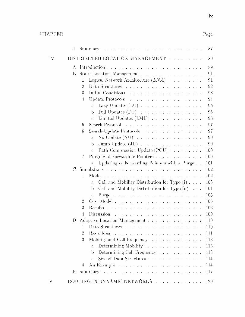
ixCHAPTER PageJ. Summary : : : : : : : : : : : : : : : : : : : : : : : : : : : 87IV DISTRIBUTED LOCATION MANAGEMENT : : : : : : : : : 89A. Introduction : : : : : : : : : : : : : : : : : : : : : : : : : : 89B. Static Location Management : : : : : : : : : : : : : : : : : 911. Logical Network Architecture (LNA) : : : : : : : : : 912. Data Structures : : : : : : : : : : : : : : : : : : : : : 923. Initial Conditions : : : : : : : : : : : : : : : : : : : : 934. Update Protocols : : : : : : : : : : : : : : : : : : : : 94a. Lazy Updates (LU) : : : : : : : : : : : : : : : : : 95b. Full Updates (FU) : : : : : : : : : : : : : : : : : 95c. Limited Updates (LMU) : : : : : : : : : : : : : : 965. Search Protocol : : : : : : : : : : : : : : : : : : : : : 976. Search-Update Protocols : : : : : : : : : : : : : : : : 97a. No Update (NU) : : : : : : : : : : : : : : : : : : 99b. Jump Update (JU) : : : : : : : : : : : : : : : : : 99c. Path Compression Update (PCU) : : : : : : : : : 1007. Purging of Forwarding Pointers : : : : : : : : : : : : : 100a. Updating of Forwarding Pointers with a Purge : : 101C. Simulations : : : : : : : : : : : : : : : : : : : : : : : : : : 1021. Model : : : : : : : : : : : : : : : : : : : : : : : : : : : 102a. Call and Mobility Distribution for Type (i) : : : : 103b. Call and Mobility Distribution for Type (ii) : : : 104c. Purge : : : : : : : : : : : : : : : : : : : : : : : : 1052. Cost Model : : : : : : : : : : : : : : : : : : : : : : : : 1063. Results : : : : : : : : : : : : : : : : : : : : : : : : : : 1064. Discussion : : : : : : : : : : : : : : : : : : : : : : : : 109D. Adaptive Location Management : : : : : : : : : : : : : : : 1101. Data Structures : : : : : : : : : : : : : : : : : : : : : 1102. Basic Idea : : : : : : : : : : : : : : : : : : : : : : : : 1113. Mobility and Call Frequency : : : : : : : : : : : : : : 113a. Determining Mobility : : : : : : : : : : : : : : : : 113b. Determining Call Frequency : : : : : : : : : : : : 113c. Size of Data Structures : : : : : : : : : : : : : : : 1144. An Example : : : : : : : : : : : : : : : : : : : : : : : 114E. Summary : : : : : : : : : : : : : : : : : : : : : : : : : : : 117V ROUTING IN DYNAMIC NETWORKS : : : : : : : : : : : : : 120

xCHAPTER PageA. Introduction : : : : : : : : : : : : : : : : : : : : : : : : : : 1201. Previous Work : : : : : : : : : : : : : : : : : : : : : : 1212. Proposed Approach : : : : : : : : : : : : : : : : : : : 124B. Preliminaries : : : : : : : : : : : : : : : : : : : : : : : : : 126C. Cluster Formation : : : : : : : : : : : : : : : : : : : : : : : 1301. Host HA Switches ON : : : : : : : : : : : : : : : : : : 1312. Host HA Switches OFF : : : : : : : : : : : : : : : : : 1383. Host HA Gets Connected to Host HB : : : : : : : : : 1424. Host HA Disconnects Host HB : : : : : : : : : : : : : 142D. Routing Protocol : : : : : : : : : : : : : : : : : : : : : : : 1431. Data Structures : : : : : : : : : : : : : : : : : : : : : 1432. Protocol : : : : : : : : : : : : : : : : : : : : : : : : : 144a. Route Construction Phase : : : : : : : : : : : : : 147b. Route Maintenance Phase : : : : : : : : : : : : : 1473. Implementation Details : : : : : : : : : : : : : : : : : 148E. Performance Evaluation : : : : : : : : : : : : : : : : : : : 1491. Complexity : : : : : : : : : : : : : : : : : : : : : : : : 1492. Simulations : : : : : : : : : : : : : : : : : : : : : : : : 152F. Other Clustering Approaches : : : : : : : : : : : : : : : : 156G. Summary : : : : : : : : : : : : : : : : : : : : : : : : : : : 157VI CONCLUSION : : : : : : : : : : : : : : : : : : : : : : : : : : : 158A. Summary of Results : : : : : : : : : : : : : : : : : : : : : 158B. Future Work : : : : : : : : : : : : : : : : : : : : : : : : : : 161REFERENCES : : : : : : : : : : : : : : : : : : : : : : : : : : : : : : : : : : : 163APPENDIX A : : : : : : : : : : : : : : : : : : : : : : : : : : : : : : : : : : : 173APPENDIX B : : : : : : : : : : : : : : : : : : : : : : : : : : : : : : : : : : : 176APPENDIX C : : : : : : : : : : : : : : : : : : : : : : : : : : : : : : : : : : : 180APPENDIX D : : : : : : : : : : : : : : : : : : : : : : : : : : : : : : : : : : : 183APPENDIX E : : : : : : : : : : : : : : : : : : : : : : : : : : : : : : : : : : : 187VITA : : : : : : : : : : : : : : : : : : : : : : : : : : : : : : : : : : : : : : : : 189

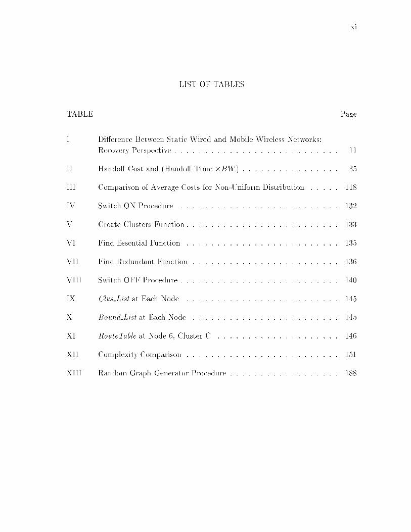
xiLIST OF TABLESTABLE PageI Di�erence Between Static Wired and Mobile Wireless Networks:Recovery Perspective : : : : : : : : : : : : : : : : : : : : : : : : : : : 11II Hando� Cost and (Hando� Time �BW ) : : : : : : : : : : : : : : : : 35III Comparison of Average Costs for Non-Uniform Distribution : : : : : 118IV Switch ON Procedure : : : : : : : : : : : : : : : : : : : : : : : : : : 132V Create Clusters Function : : : : : : : : : : : : : : : : : : : : : : : : : 133VI Find Essential Function : : : : : : : : : : : : : : : : : : : : : : : : : 135VII Find Redundant Function : : : : : : : : : : : : : : : : : : : : : : : : 136VIII Switch OFF Procedure : : : : : : : : : : : : : : : : : : : : : : : : : : 140IX Clus List at Each Node : : : : : : : : : : : : : : : : : : : : : : : : : 145X Bound List at Each Node : : : : : : : : : : : : : : : : : : : : : : : : 145XI RouteTable at Node 6, Cluster C : : : : : : : : : : : : : : : : : : : : 146XII Complexity Comparison : : : : : : : : : : : : : : : : : : : : : : : : : 151XIII Random Graph Generator Procedure : : : : : : : : : : : : : : : : : : 188

xiiLIST OF FIGURESFIGURE Page1 Classi�cation of Wireless Networks : : : : : : : : : : : : : : : : : : : 122 Best Recovery Scheme : : : : : : : : : : : : : : : : : : : : : : : : : : 143 Hando� in the Middle of an Execution : : : : : : : : : : : : : : : : : 184 Markov Chain Representation : : : : : : : : : : : : : : : : : : : : : : 245 State Intervals : : : : : : : : : : : : : : : : : : : : : : : : : : : : : : 256 koptLL vs. r and �: � = 10�2, = 0:1 : : : : : : : : : : : : : : : : : : 337 koptLL vs. and �: � = 10, r = 0:1 : : : : : : : : : : : : : : : : : : : 348 Recovery Cost: � = 10�2, � = 10 : : : : : : : : : : : : : : : : : : : : 369 Total Cost: � = 10�2, � = 10 : : : : : : : : : : : : : : : : : : : : : : 3810 Total Cost: � = 10�5, � = 10 : : : : : : : : : : : : : : : : : : : : : : 3911 Total Cost: � = 10�2, � = 500 : : : : : : : : : : : : : : : : : : : : : 3912 Best Location Management Scheme : : : : : : : : : : : : : : : : : : : 4413 Update in the Basic Scheme (IS-41) : : : : : : : : : : : : : : : : : : 4814 Search in the Basic Scheme (IS-41) : : : : : : : : : : : : : : : : : : : 4915 An Example of Forwarding Tree : : : : : : : : : : : : : : : : : : : : : 5216 Search using HLS and Forwarding Pointers : : : : : : : : : : : : : : 5417 Maximum Allowable Chain Length : : : : : : : : : : : : : : : : : : : 6318 Relative Total Costs: � = 0:2 : : : : : : : : : : : : : : : : : : : : : : 6419 Relative Total Costs: � = 0:5 : : : : : : : : : : : : : : : : : : : : : : 64

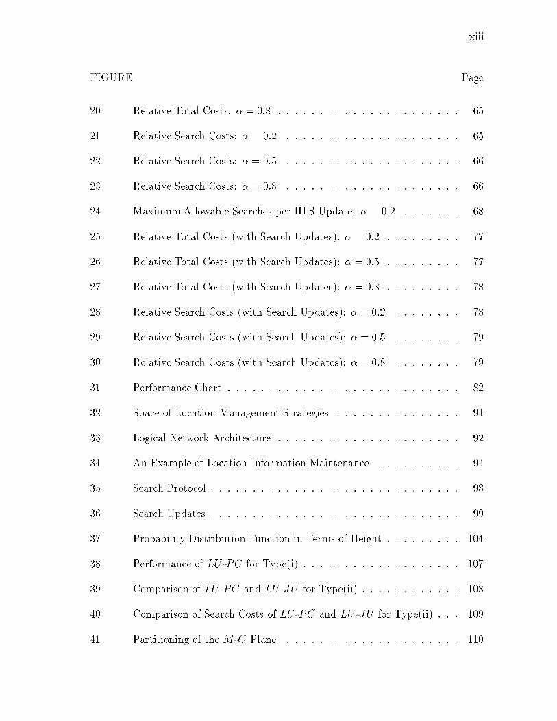
xiiiFIGURE Page20 Relative Total Costs: � = 0:8 : : : : : : : : : : : : : : : : : : : : : : 6521 Relative Search Costs: � = 0:2 : : : : : : : : : : : : : : : : : : : : : 6522 Relative Search Costs: � = 0:5 : : : : : : : : : : : : : : : : : : : : : 6623 Relative Search Costs: � = 0:8 : : : : : : : : : : : : : : : : : : : : : 6624 Maximum Allowable Searches per HLS Update: � = 0:2 : : : : : : : 6825 Relative Total Costs (with Search Updates): � = 0:2 : : : : : : : : : 7726 Relative Total Costs (with Search Updates): � = 0:5 : : : : : : : : : 7727 Relative Total Costs (with Search Updates): � = 0:8 : : : : : : : : : 7828 Relative Search Costs (with Search Updates): � = 0:2 : : : : : : : : 7829 Relative Search Costs (with Search Updates): � = 0:5 : : : : : : : : 7930 Relative Search Costs (with Search Updates): � = 0:8 : : : : : : : : 7931 Performance Chart : : : : : : : : : : : : : : : : : : : : : : : : : : : : 8232 Space of Location Management Strategies : : : : : : : : : : : : : : : 9133 Logical Network Architecture : : : : : : : : : : : : : : : : : : : : : : 9234 An Example of Location Information Maintenance : : : : : : : : : : 9435 Search Protocol : : : : : : : : : : : : : : : : : : : : : : : : : : : : : : 9836 Search Updates : : : : : : : : : : : : : : : : : : : : : : : : : : : : : : 9937 Probability Distribution Function in Terms of Height : : : : : : : : : 10438 Performance of LU -PC for Type(i) : : : : : : : : : : : : : : : : : : : 10739 Comparison of LU -PC and LU -JU for Type(ii) : : : : : : : : : : : : 10840 Comparison of Search Costs of LU -PC and LU -JU for Type(ii) : : : 10941 Partitioning of the M -C Plane : : : : : : : : : : : : : : : : : : : : : 110

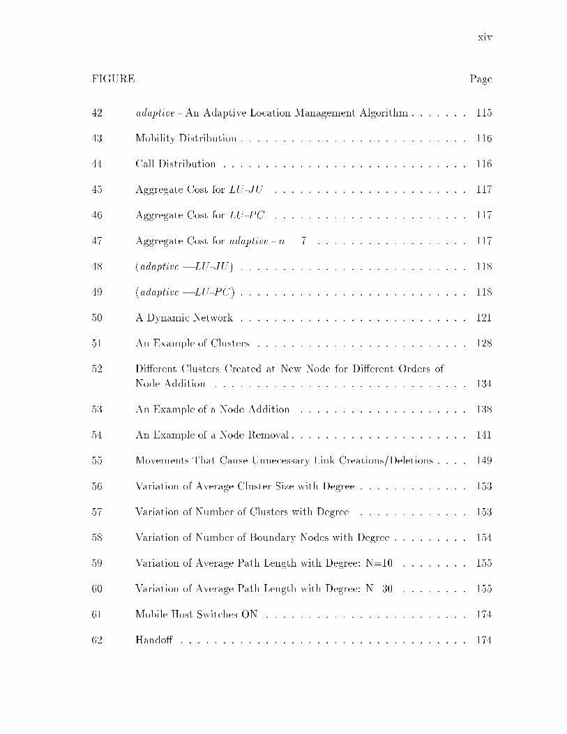
xivFIGURE Page42 adaptive - An Adaptive Location Management Algorithm : : : : : : : 11543 Mobility Distribution : : : : : : : : : : : : : : : : : : : : : : : : : : : 11644 Call Distribution : : : : : : : : : : : : : : : : : : : : : : : : : : : : : 11645 Aggregate Cost for LU -JU : : : : : : : : : : : : : : : : : : : : : : : 11746 Aggregate Cost for LU -PC : : : : : : : : : : : : : : : : : : : : : : : 11747 Aggregate Cost for adaptive - n = 7 : : : : : : : : : : : : : : : : : : 11748 (adaptive � LU -JU) : : : : : : : : : : : : : : : : : : : : : : : : : : : 11849 (adaptive � LU -PC) : : : : : : : : : : : : : : : : : : : : : : : : : : : 11850 A Dynamic Network : : : : : : : : : : : : : : : : : : : : : : : : : : : 12151 An Example of Clusters : : : : : : : : : : : : : : : : : : : : : : : : : 12852 Di�erent Clusters Created at New Node for Di�erent Orders ofNode Addition : : : : : : : : : : : : : : : : : : : : : : : : : : : : : : 13453 An Example of a Node Addition : : : : : : : : : : : : : : : : : : : : 13854 An Example of a Node Removal : : : : : : : : : : : : : : : : : : : : : 14155 Movements That Cause Unnecessary Link Creations/Deletions : : : : 14956 Variation of Average Cluster Size with Degree : : : : : : : : : : : : : 15357 Variation of Number of Clusters with Degree : : : : : : : : : : : : : 15358 Variation of Number of Boundary Nodes with Degree : : : : : : : : : 15459 Variation of Average Path Length with Degree: N=10 : : : : : : : : 15560 Variation of Average Path Length with Degree: N=30 : : : : : : : : 15561 Mobile Host Switches ON : : : : : : : : : : : : : : : : : : : : : : : : 17462 Hando� : : : : : : : : : : : : : : : : : : : : : : : : : : : : : : : : : : 174

xvFIGURE Page63 State Transitions when Search-Updates are used with Movement-based Heuristic : : : : : : : : : : : : : : : : : : : : : : : : : : : : : : 17764 Variation of k0 with r for M = 3 : : : : : : : : : : : : : : : : : : : : 17865 Variation of s with r for M = 3 : : : : : : : : : : : : : : : : : : : : : 17866 State Transitions when Search-Updates are used with Search-based Heuristic : : : : : : : : : : : : : : : : : : : : : : : : : : : : : : 18167 Variation of k' with r (Search-based) for N=50 : : : : : : : : : : : : 18168 Variation of s with r (Search-based) for N=50 : : : : : : : : : : : : : 18269 Clusters formed by Find-Essential : : : : : : : : : : : : : : : : : : 185

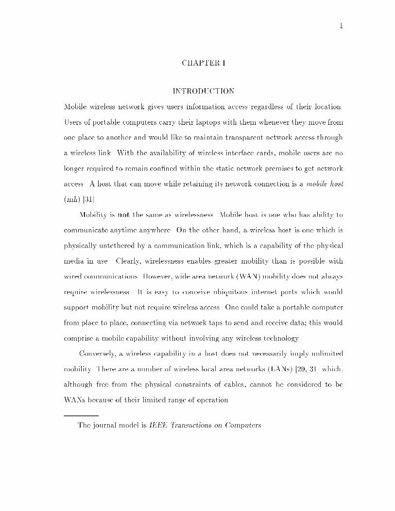
1CHAPTER IINTRODUCTIONMobile wireless network gives users information access regardless of their location.Users of portable computers carry their laptops with them whenever they move fromone place to another and would like to maintain transparent network access througha wireless link. With the availability of wireless interface cards, mobile users are nolonger required to remain con�ned within the static network premises to get networkaccess. A host that can move while retaining its network connection is a mobile host(mh) [31].Mobility is not the same as wirelessness. Mobile host is one who has ability tocommunicate anytime anywhere. On the other hand, a wireless host is one which isphysically untethered by a communication link, which is a capability of the physicalmedia in use. Clearly, wirelessness enables greater mobility than is possible withwired communications. However, wide area network (WAN) mobility does not alwaysrequire wirelessness. It is easy to conceive ubiquitous internet ports which wouldsupport mobility but not require wireless access. One could take a portable computerfrom place to place, connecting via network taps to send and receive data; this wouldcomprise a mobile capability without involving any wireless technology.Conversely, a wireless capability in a host does not necessarily imply unlimitedmobility. There are a number of wireless local area networks (LANs) [20, 31] which,although free from the physical constraints of cables, cannot be considered to beWANs because of their limited range of operation.The journal model is IEEE Transactions on Computers.

2A. Classi�cation of Mobile Wireless NetworksMobile wireless networks can be classi�ed broadly into two types : Infrastructurenetworks and Dynamic networks.1. Infrastructure NetworksInfrastructure networks are two tiered networks composed of a static backbone net-work and peripheral wireless networks [9, 51, 58]. The static network comprises of�xed hosts and communication links between them. Some of the �xed hosts, calledmobile support stations (MSS)1 are augmented with a wireless interface, and, theyprovide a gateway for communication between the wireless network and the staticnetwork. Due to the limited range of wireless transceivers, a mobile host can commu-nicate with a mobile support station only within a limited geographical region aroundit. This region is referred to as a mobile support station's cell. A mobile host com-municates with one MSS at any given time. MSS is responsible for forwarding databetween the mobile host and static network. Communication to and from the mobilehost takes place via the static network. An example of infrastructure networks is thenew Personal Communication Systems (PCS) [20, 31].2. Dynamic NetworksDynamic networks consist of mobile hosts which can communicate with each otherover the wireless links (direct or indirect) without any static network interaction.In such networks the mobile host has the capability to communicate directly withanother mobile host in its vicinity. The mobile hosts also have the capability toforward (relay) packets. Examples of such networks are ad-hoc wireless local area1Mobile support stations are also called base stations.

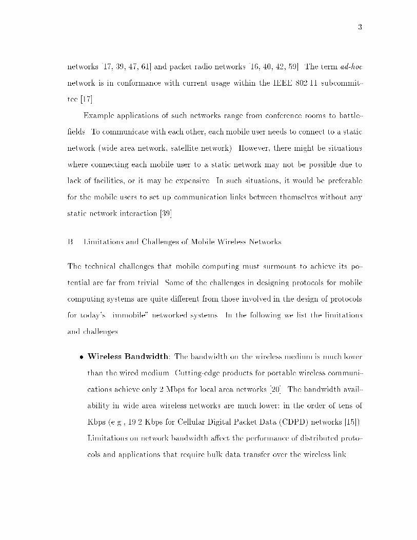
3networks [17, 39, 47, 61] and packet radio networks [16, 40, 42, 59]. The term ad-hocnetwork is in conformance with current usage within the IEEE 802.11 subcommit-tee [17].Example applications of such networks range from conference rooms to battle-�elds. To communicate with each other, each mobile user needs to connect to a staticnetwork (wide area network, satellite network). However, there might be situationswhere connecting each mobile user to a static network may not be possible due tolack of facilities, or it may be expensive. In such situations, it would be preferablefor the mobile users to set up communication links between themselves without anystatic network interaction [39].B. Limitations and Challenges of Mobile Wireless NetworksThe technical challenges that mobile computing must surmount to achieve its po-tential are far from trivial. Some of the challenges in designing protocols for mobilecomputing systems are quite di�erent from those involved in the design of protocolsfor today's \immobile" networked systems. In the following we list the limitationsand challenges.� Wireless Bandwidth: The bandwidth on the wireless medium is much lowerthan the wired medium. Cutting-edge products for portable wireless communi-cations achieve only 2 Mbps for local area networks [20]. The bandwidth avail-ability in wide area wireless networks are much lower; in the order of tens ofKbps (e.g., 19.2 Kbps for Cellular Digital Packet Data (CDPD) networks [15]).Limitations on network bandwidth a�ect the performance of distributed proto-cols and applications that require bulk data transfer over the wireless link.

4� Unreliable Wireless Link: While the wired links on the static network o�era virtually error free transmission medium (Bit Error Rates (BER) of the orderof 10�8 to 10�12), wireless links are much more unreliable. BER in wirelesslinks is of the order of 10�2 to 10�6, and they are highly sensitive to the direc-tion of propagation, multipath fading, and other interference [9, 51]. Networkprotocols such as TCP, ATM do not work well in wireless networks becausethey were tailored for environments which o�er a relatively stable and error freetransmission medium, unlike the much more hostile and error prone wirelessmedium [6, 7, 8, 14].� Mobility of Hosts: Wireless connection enables virtually unrestricted mobilityand connectivity from any location within the area of radio coverage. Mobilityis an important new component that will have far-reaching consequences forsystem design. An important issue that stems out of mobility of hosts is designand analysis of location management schemes in infrastructure networks [36,37, 49, 50, 57, 58]. In dynamic networks, mobility of hosts causes the networktopology to change. This in turn complicates the design of routing protocols insuch networks [16, 39, 47, 59, 61]. Mobility also a�ects the design of applications.In a client-server environment, mobile clients may �nd themselves far away fromtheir servers; servers may also move further away from their clients. Thus, thesystem will have to adapt to changing spatial distribution of clients by dynamicreplication of data and services (for example [31]).� Available Storage on Mobile Computers: The storage space available ona mobile computer is limited by physical size and power requirements. Tradi-tionally, disks provide large amounts of stable (non-volatile) storage. However,in a mobile computer, disks are a liability. This is because, they consume more

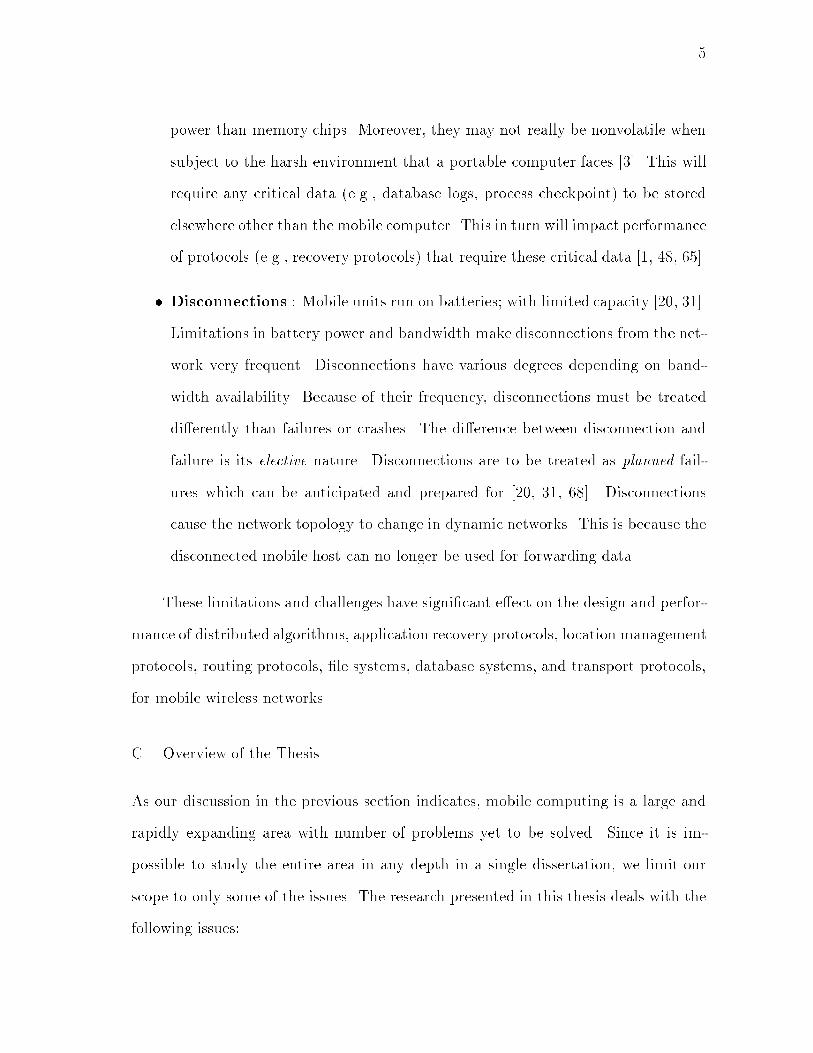
5power than memory chips. Moreover, they may not really be nonvolatile whensubject to the harsh environment that a portable computer faces [3]. This willrequire any critical data (e.g., database logs, process checkpoint) to be storedelsewhere other than the mobile computer. This in turn will impact performanceof protocols (e.g., recovery protocols) that require these critical data [1, 48, 65].� Disconnections : Mobile units run on batteries; with limited capacity [20, 31].Limitations in battery power and bandwidth make disconnections from the net-work very frequent. Disconnections have various degrees depending on band-width availability. Because of their frequency, disconnections must be treateddi�erently than failures or crashes. The di�erence between disconnection andfailure is its elective nature. Disconnections are to be treated as planned fail-ures which can be anticipated and prepared for [20, 31, 68]. Disconnectionscause the network topology to change in dynamic networks. This is because thedisconnected mobile host can no longer be used for forwarding data.These limitations and challenges have signi�cant e�ect on the design and perfor-mance of distributed algorithms, application recovery protocols, location managementprotocols, routing protocols, �le systems, database systems, and transport protocols,for mobile wireless networks.C. Overview of the ThesisAs our discussion in the previous section indicates, mobile computing is a large andrapidly expanding area with number of problems yet to be solved. Since it is im-possible to study the entire area in any depth in a single dissertation, we limit ourscope to only some of the issues. The research presented in this thesis deals with thefollowing issues:

6� Application level recovery in infrastructure networks� Location management in infrastructure networks� Routing in dynamic networks1. Recovery IssuesThe mobile computing environment poses challenging fault-tolerant data managementproblems due to the mobility of the users, limited bandwidth on the wireless link,and power restrictions on the mobile hosts. Thus, traditional fault-tolerance schemescannot be directly applied to these systems. In this work we investigate the limitationsof the mobile wireless environment, and its impact on recovery protocols. To thise�ect, extensions to existing traditional recovery schemes are presented which suitthis environment. We build analytical models to analyze the performance of theseschemes to determine those environments where a particular recovery scheme is bestsuited. The trade-o� parameters to evaluate the recovery scheme are identi�ed. Itis determined that in addition to the failure rate of the host, the performance of arecovery scheme depended on the mobility of the hosts and the wireless bandwidth.2. Location ManagementAn important issue in personal communication networks is the design and analysisof location management schemes. We classify the location management schemes intocentralized and distributed schemes.a. Centralized Location ManagementCentralized location management schemes assume that each host has a home servernamed the home location server (HLS) which maintains the current location of the

7host. There are existing standards for carrying out location management in a central-ized manner, e.g., EIA/TIA Interim Standard 41 (IS-41) [58]. However, these schemesare not e�cient, due to increase in network load and location management costs. Toovercome these drawbacks, we propose forwarding techniques that augment the IS-41scheme to provide e�cient location management. Although, forwarding reduces net-work load during updates, they may increase search cost due to long chain lengths.We propose heuristics to limit the number of forwarding pointers traversed during asearch. We build analytical models to compare the performance of the proposed ap-proach with the IS-41 scheme. We also present a strategy to perform search-updates.A search-update occurs after a successful search, when the location information cor-responding to the searched mobile host is updated at some hosts. Analysis shows thatfor some network parameter values, performing search-updates signi�cantly reducesthe search costs and total network load.b. Distributed Location ManagementStudies have indicated that in centralized location management schemes such as IS-41, the bottleneck is the HLS [57, 58]. For a typical PCS environment, the HLS isexpected to experience a high update rate, and a very high search (or call-delivery)rate [58]. It is thus evident that new network architectures need to be investigatedfor PCS. In this work we use a network architecture that consists of a hierarchy oflocation servers so that there is no single bottleneck in the network. We propose staticand adaptive location management schemes for this network architecture. A suite ofschemes is proposed, however, it is observed that no scheme outperforms others forall call-mobility patterns. Thus, in order to obtain good performance using staticlocation management, the system designer should a priori have a fair idea of thecall-mobility pattern of the users. However, the user behavior is not always available

8to the system designer. Thus, there is a need for adaptive location management.We propose an adaptive scheme that dynamically estimates the future user behaviorwith the help of past call-mobility patterns. Results indicate that the adaptive schemeperforms better than the static schemes for a wide range of call-mobility patterns.3. Routing ProtocolThe design and analysis of routing protocols is an important issue in dynamic net-works such as packet radio and ad-hoc wireless networks. The conventional routingprotocols were not designed for networks where the topological connectivity is subjectto frequent, unpredictable changes. Most protocols exhibit their least desirable be-havior for highly dynamic interconnection topology. We propose a new methodologyfor routing and topology information maintenance in dynamic networks. The basicidea behind the protocol is to divide the graph into number of overlapping clusters.A change in the network topology corresponds to a change in cluster membership.We present algorithms for creation of clusters, as well as algorithms to maintain themin the presence of various network events. Compared to existing and conventionalrouting protocols, the proposed cluster-based approach incurs lower overhead duringtopology updates and also has quicker reconvergence. The e�ectiveness of this ap-proach also lies in the fact that existing routing protocols can be directly applied tothe network { replacing the nodes by clusters.D. Thesis OrganizationIn Chapter II we address the recovery issues in mobile wireless networks. Chapter IIIpresents the centralized location management scheme. Chapter IV presents the dis-tributed location management scheme. The cluster-based approach for routing in

9dynamic networks is presented in Chapter V. Chapter VI summarizes the results ofthis thesis and discusses possible extensions.

10CHAPTER IIRECOVERY IN MOBILE ENVIRONMENTA. IntroductionThis chapter deals with design of protocols to recover from a mobile host failure inan infrastructure mobile wireless network. The system model of the infrastructurenetwork is the same as explained in Chapter I.A mobile host may become unavailable due to (i) failure of the mobile host, (ii)disconnection of the mobile host, and (iii) wireless link failure [20, 31, 48, 65]. Loss ofbattery power make disconnections from the network frequent, and sometimes unpre-dictable. Because of their frequency, disconnections must be treated di�erently thanfailures. The di�erence between disconnection and failure is its elective nature. Userinitiated disconnections can be treated as planned failures, which can be anticipatedand prepared for [20, 31, 68]. The wireless link is equivalent to an intermittentlyfaulty link, which transmits correct messages during fault-free conditions, and stopsany transmissions upon a failure. Disconnections and weak wireless links primarilydelay the system response, whereas a host failure a�ects the system state.Strategies are developed in this paper to recover from various transient faultsin the mobile host. These are faults that are typically caused by environmentalupsets (e.g., wireless link failure, power glitches at the mobile host, electromagneticinterference, radiation, etc.) or software errors (e.g., heisenbugs [38], rarely used codepaths, etc.). Transient failures are the most common mode of failure [64]. We assumethe well known fail-silent [64] model. In this model, upon a failure at a mobile host,the host stops executing, and its state is lost. Failure detection is performed byrequiring a mobile host to send periodic \I am alive" messages to the base station.

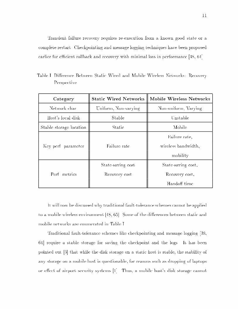
11Transient failure recovery requires re-execution from a known good state or acomplete restart. Checkpointing and message logging techniques have been proposedearlier for e�cient rollback and recovery with minimal loss in performance [38, 64].Table I. Di�erence Between Static Wired and Mobile Wireless Networks: RecoveryPerspectiveCategory Static Wired Networks Mobile Wireless NetworksNetwork char. Uniform, Non-varying Non-uniform, VaryingHost's local disk Stable UnstableStable storage location Static MobileFailure rate,Key perf. parameter Failure rate wireless bandwidth,mobilityState-saving cost State-saving cost,Perf. metrics Recovery cost Recovery cost,Hando� timeIt will now be discussed why traditional fault-tolerance schemes cannot be appliedto a mobile wireless environment [48, 65]. Some of the di�erences between static andmobile networks are enumerated in Table I.Traditional fault-tolerance schemes like checkpointing and message logging [38,64] require a stable storage for saving the checkpoint and the logs. It has beenpointed out [3] that while the disk storage on a static host is stable, the stability ofany storage on a mobile host is questionable, for reasons such as dropping of laptopsor e�ect of airport security systems [1]. Thus, a mobile host's disk storage cannot

12be considered stable and is vulnerable to failures. Moreover, all mobile hosts arenot necessarily equipped with disk storage. Thus, we need the stable storage to belocated on a static host. An obvious candidate is the `local base station', that isthe base station in charge of the cell in which the mobile host is currently residing.Traditional recovery schemes are not applicable because the mobile hosts move fromcell to cell. Thus, a mobile host does not have a �xed base station to communicatewith. Also, recovery is complicated because successive checkpoints of a mobile hostmay be stored at di�erent base stations. This dynamic topological situation warrantsformulation of special techniques to recover from failures.Wireless Networks

In-Building Campus Area Wide Area Regional Area

Wireless LAN,Infrared

AsynchronousUp: < 10 Kbps

Down: > 1 Mbps

VehicularPedestrianStationary

VehicularPedestrian

10-30 Kbps> 64 Kbps

PedestrianPedestrian

> 1 Mbps

Mobility

Bandwidth

Medium Packet Relay Cellular Satellite

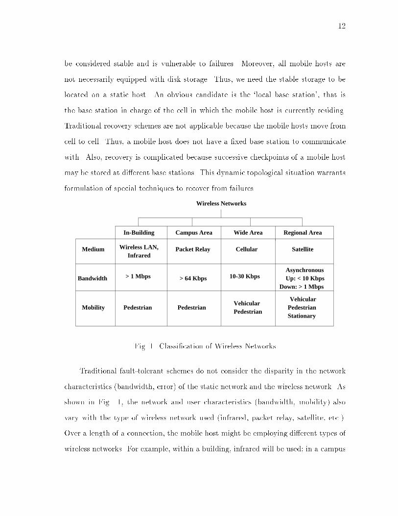
Fig. 1. Classi�cation of Wireless NetworksTraditional fault-tolerant schemes do not consider the disparity in the networkcharacteristics (bandwidth, error) of the static network and the wireless network. Asshown in Fig. 1, the network and user characteristics (bandwidth, mobility) alsovary with the type of wireless network used (infrared, packet relay, satellite, etc.).Over a length of a connection, the mobile host might be employing di�erent types ofwireless networks. For example, within a building, infrared will be used; in a campus

13environment, packet relay will be used; and in a remote region, satellite will be used.Available wireless bandwidth and error conditions will be di�erent in each of thesewireless networks. Thus, the appropriate recovery protocol needs to be determinedadaptively, based on the characteristics of the underlying wireless network and users.Performance of traditional recovery schemes primarily depends on the failure rateof the host [63, 77]. However, in a mobile environment, due to mobility of the hostsand limited bandwidth on the wireless links, parameters other than failure rate of themobile host play a key role in determining the e�ectiveness of a recovery scheme. Amobile environment is determined by the mobility, wireless bandwidth and the failurerate. This chapter presents the following:� User transparent recovery from mobile host failure.� Trade-o�s for the recovery schemes proposed.� Best recovery scheme for an environment.We propose several schemes for recovery from a failure of a mobile host. Theseproposed schemes have two major components: a state-saving scheme and a hando�scheme. We propose two schemes for state-saving, namely, (i) No Logging (N) and (ii)Logging (L), and three schemes for hando�, namely, (i) Pessimistic (P ), (ii) Lazy (L),and (iii) Trickle (T ). We denote a recovery scheme that employs a combination of astate-saving scheme, X (X 2 fN;Lg), and a hando� scheme, Y (Y 2 fP;L; Tg), asXY . For example, LL is a recovery scheme that uses a combination of the Loggingscheme for state-saving and the Lazy scheme for hando�s.Each combination provides some level of availability and requires some amountof resources: network bandwidth, memory, and processing power. Through analysis,we show that there can be no single recovery scheme that performs well for all mobile

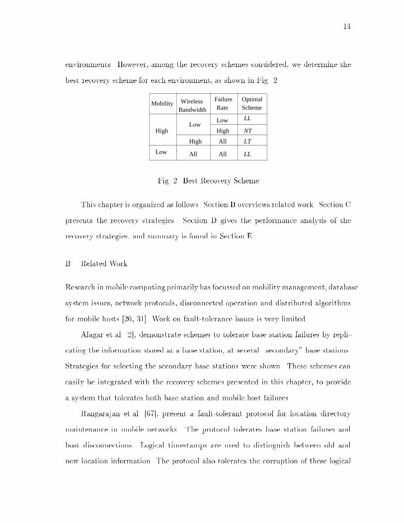
14environments. However, among the recovery schemes considered, we determine thebest recovery scheme for each environment, as shown in Fig. 2.Low

All

Mobility Wireless Failure

Low

High

All

All

Bandwidth RateOptimalScheme

LL

NT

LTHigh

LLLow

HighFig. 2. Best Recovery SchemeThis chapter is organized as follows. Section B overviews related work. Section Cpresents the recovery strategies. Section D gives the performance analysis of therecovery strategies, and summary is found in Section E.B. Related WorkResearch in mobile computing primarily has focussed on mobilitymanagement, databasesystem issues, network protocols, disconnected operation and distributed algorithmsfor mobile hosts [20, 31]. Work on fault-tolerance issues is very limited.Alagar et.al. [2], demonstrate schemes to tolerate base station failures by repli-cating the information stored at a base station, at several \secondary" base stations.Strategies for selecting the secondary base stations were shown. These schemes caneasily be integrated with the recovery schemes presented in this chapter, to providea system that tolerates both base station and mobile host failures.Rangarajan et.al. [67], present a fault-tolerant protocol for location directorymaintenance in mobile networks. The protocol tolerates base station failures andhost disconnections. Logical timestamps are used to distinguish between old andnew location information. The protocol also tolerates the corruption of these logical

15timestamps.Lin [52], studies the recovery of mobility databases at the visitor location regis-ter (V LR) and home location register (HLR) for personal communication networks.Schemes with and without checkpointing are described and analyzed.Acharya et.al. [1], identify the problems with checkpointing mobile distributedapplications, presenting an algorithm for recording global checkpoints for distributedapplications running on mobile hosts.In this research, however, we consider protocols to recover from failure in a mobilehost, independent of other hosts in the system. Also, we study the e�ect of mobilityand wirelessness on such recovery protocols.C. Recovery StrategiesA recovery strategy essentially has two components: a state-saving and a hando�strategy. This Section presents two strategies for saving the state, and three strategiesfor hando�, to achieve fault-tolerance. Strategies for saving the state are similar totraditional fault-tolerance strategies.1. State-SavingState-saving strategies presented in this chapter are based on traditional checkpoint-ing and message-logging techniques. In such strategies, the host periodically saves itsstate at a stable storage. Thus, upon failure of the host, execution can be restartedfrom the last-saved checkpoint.It was indicated earlier [3] that a mobile host's disk storage cannot be consideredstable. Thus, our algorithms use the storage available at the base station for the cellin which the mobile host is currently residing, as the stable storage.

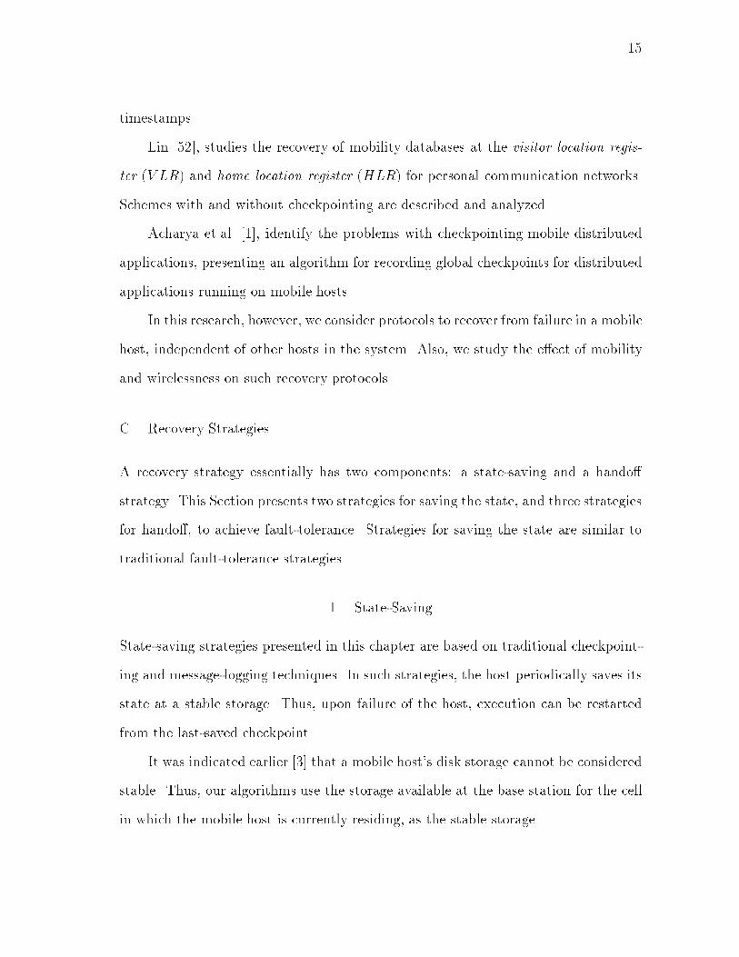
16Multiple hosts (both static and mobile) will take part in a distributed application.Such applications require messages to be transferred between the hosts, and mightalso require user inputs at the mobile hosts. While the user inputs may go directlyto the mobile host, the messages will �rst reach the base station in charge of thecell in which the mobile host currently resides. The base station then forwards themessages to the corresponding mobile host. Likewise, all messages sent by a mobilehost will �rst be sent to its base station, which will forward them to the destinationhost (static or mobile).Two strategies to save the process state [38] will be discussed here: (i) No Loggingand (ii) Logging. It is assumed that the mobile host remains in one cell during thelength of the application. This is followed by a discussion of three schemes thataddress the recovery steps needed because of mobility.� No Logging Approach (denoted as N): The state of the process can get altered,either upon receipt of a message from another host, or upon user input. The messagesor inputs that modify the state are called write events. (If semantics of the messageare not known, in the worst case, we might have to assume that the state gets alteredupon receipt of every message or user input). In the No Logging approach, the stateof the mobile host is saved at the base station upon every write event on the mobilehost data.After a failure, when the mobile host restarts, the host sends a message to thebase station, which then transfers the latest state to the mobile host. The mobilehost then loads the latest state and resumes operation. Importantly, need for frequenttransmission of state on the wireless link is a limiting factor for this scheme.� Logging Approach (denoted as L): This approach is rooted in \pessimistic" log-ging [13], used in static systems. In this scheme, a mobile host checkpoints its stateperiodically. To facilitate recovery, the write events that take place in the interval

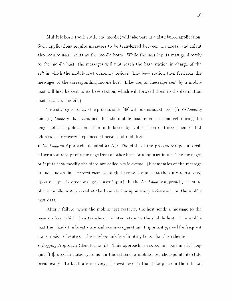
17between checkpoints are also logged. As de�ned earlier, the messages or inputs thatmodify the state of the mobile host are called write events. If a write message isreceived from another host, the base station �rst logs it, and then forwards it to themobile host for execution. Likewise, upon user input (write event), the mobile host�rst forwards a copy of the user input to the base station, for logging. After log-ging, the base station sends an acknowledgment back to the mobile host. The mobilehost can process the input, while waiting for the acknowledgment, but cannot senda response. Only upon receipt of the acknowledgment does the mobile host send itsresponse.The above procedure ensures that no messages or user inputs are lost due toa failure of the mobile host. The logging of the write events continues until a newcheckpoint is backed up at the base station. The base station then purges the log ofthe old write events, along with the previous checkpoint.After a failure, when the mobile host restarts, the host sends a message to thebase station, which then transfers both the latest backed-up checkpoint of the host,as well as the log of write events, to the mobile host. The mobile host then loadsthe latest backed-up checkpoint and restarts executing, by replaying the write eventsfrom its logs, thus reaching the state before failure. Below, the recovery steps areconsidered which are needed, arising due to mobility of the hosts.2. Hando�The mobility warrants a special hando� process, described below. The key problemto be addressed is how a recovery can be e�ected if a mobile host moves to a newcell, as illustrated in the following example.Consider the system in Fig. 3. BSi denotes i-th base station, and mhi denotesi-th mobile host. Here, mobile hosts mh1 and mh2 are executing a distributed algo-

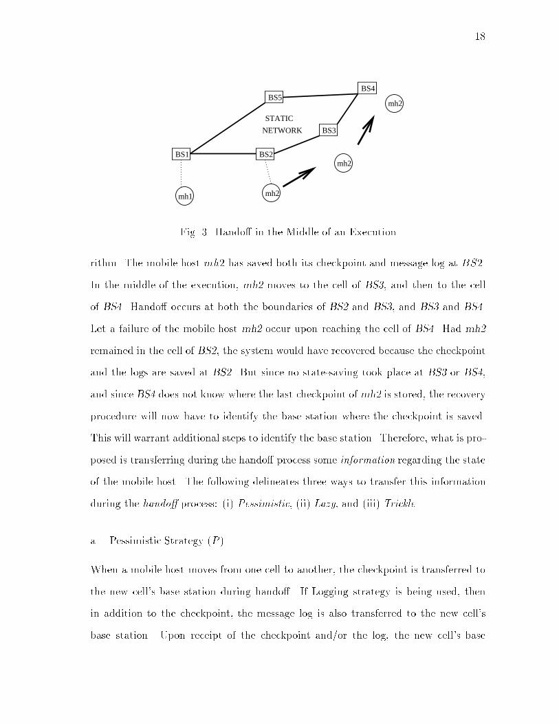
18mh2

mh2

NETWORK

STATIC

BS5

mh2mh1

BS4

BS3

BS2BS1Fig. 3. Hando� in the Middle of an Executionrithm. The mobile host mh2 has saved both its checkpoint and message log at BS2.In the middle of the execution, mh2 moves to the cell of BS3, and then to the cellof BS4. Hando� occurs at both the boundaries of BS2 and BS3, and BS3 and BS4.Let a failure of the mobile host mh2 occur upon reaching the cell of BS4. Had mh2remained in the cell of BS2, the system would have recovered because the checkpointand the logs are saved at BS2. But since no state-saving took place at BS3 or BS4,and since BS4 does not know where the last checkpoint of mh2 is stored, the recoveryprocedure will now have to identify the base station where the checkpoint is saved.This will warrant additional steps to identify the base station. Therefore, what is pro-posed is transferring during the hando� process some information regarding the stateof the mobile host. The following delineates three ways to transfer this informationduring the hando� process: (i) Pessimistic, (ii) Lazy, and (iii) Trickle.a. Pessimistic Strategy (P )When a mobile host moves from one cell to another, the checkpoint is transferred tothe new cell's base station during hando�. If Logging strategy is being used, thenin addition to the checkpoint, the message log is also transferred to the new cell'sbase station. Upon receipt of the checkpoint and/or the log, the new cell's base

19station sends an acknowledgment to the old base station. The old base station, uponreceiving the acknowledgment, purges its copy of the checkpoint and the log, sincethe mobile host is no longer in its cell.The chief disadvantage to this approach is that it requires a large volume of datato be transferred during each hando�. Potentially, this can cause long disruptionsduring hando�s. However it can be avoided if we use the Lazy or Trickle strategy, asexplained.b. Lazy Strategy (L)With Lazy strategy, during hando�, there is no transfer of checkpoint and log. In-stead, the Lazy strategy creates a linked list of base stations of the cells visited bythe mobile host. The mobile host may be using either one of the state-saving strate-gies (No Logging or Logging) described earlier. If the mobile host is using the NoLogging strategy, the checkpoint is saved at the current cell's base station after everywrite event. On the other hand, if Logging strategy is used, a log of write events ismaintained, in addition to the last checkpoint of the mobile host at the base station.Upon a hando�, the new cell's base station keeps a record of the preceding cell. Thus,as a mobile host moves from cell to cell, the corresponding base stations e�ectivelyform a linked list. One such linked list needs to be maintained at the base station foreach mobile host.This strategy could lead to a problem if the checkpoint and logs of the mobilehost are unnecessarily saved at di�erent base stations. To avoid this, upon taking acheckpoint at a base station, a noti�cation is sent to the last cell's base station, topurge the checkpoint and logs of the mobile host, if present. If a checkpoint is notpresent, this base station forwards the noti�cation to the preceding base station inthe linked list. This process continues, until a base station with an old checkpoint of

20the mobile host is encountered. All base stations receiving the noti�cation purge anystate associated with the particular mobile host.The Lazy strategy saves considerable network overhead during hando�, comparedto the Pessimistic strategy. Recovery, though, is more complicated. Upon a failure, ifthe base station does not have the process state, it obtains the logs and the checkpointfrom the base stations in the linked list. The base station then transfers the checkpointand the log of write events to the mobile host. The host then loads the checkpoint,and replays the messages from the logs to reach the state just before failure.c. Trickle Strategy (T )Importantly, in the Lazy strategy, the scattering of logs in di�erent base stationsincreases as the mobility of the host increases, potentially making recovery time-consuming. Moreover, a failure at any one base station containing the log renders theentire state information useless.To avoid this, a Trickle strategy is proposed. In this strategy, steps are taken toensure that the logs and the checkpoint are always at a nearby base station (whichmay not be the current base station). In addition, care is taken so that the hando�time is as low as with Lazy strategy.We make sure that the logs and the checkpoint corresponding to the mobile hostare at the \preceding base station" of the current base station1. (The preceding basestation is the base station of the previous cell visited by the mobile host.) Thus,assuming that neighboring base stations are one hop from each other (on the staticnetwork), the checkpoint and the logs are always, at most, one hop from the currentbase station.1Variations of this scheme are possible where the checkpoint and logs are at abounded distance from current cell.

21To achieve the above, during hando�, a control message is sent to the precedingbase station to transfer any checkpoint or logs that had been stored for the particularmobile host. Similar to Lazy strategy, the current base station also sends a controlmessage to the new cell's base station identifying the preceding cell location of themobile host. Thus, the new cell's base station, just retains the identi�cation of themobile host's preceding cell.If a checkpoint is taken at the current base station, it sends a noti�cation to thepreceding base station that has the last checkpoint and logs, to purge the processstate of the mobile host. During recovery, if the current base station does not have acheckpoint of the process, it obtains the checkpoint and/or the logs from the precedingbase station2. The base station then transfers the checkpoint and/or the log to themobile host. The mobile host then loads the checkpoint and replays the messagesfrom the logs, to reach the state just before failure.D. Performance AnalysisBasically, six schemes (combinations of state-saving and hando�) are possible. ThisSection analyzes these schemes, determining which combination is best-suited for agiven environment. 1. Terms and NotationsThe following terminology is used, the signi�cance of which will be clearer later inthis Section.2If No Logging strategy was used for state-saving, the checkpoint will be trans-ferred. On the other hand, if Logging is used, the checkpoint and the log aretransferred.

22� The term operation may refer to one of (i) checkpointing, (ii) logging, (iii)hando�, or (iv) recovery.� Cost of an operation quanti�es the network usage of the messages due to theoperation. In other words, it is the amount of time the network is busy trasmit-ting the messages.� �: Failure rate of the mobile host. We assume that the time interval betweentwo failures follows an exponential distribution with a mean of 1=�.� �: Hando� rate of the host. We assume that the time interval between twohando�s follows an exponential distribution with a mean of T = 1=�.� The time interval between two consecutive write events is assumed to be �xedand equal to 1=�. Write events are comprised of user inputs and messagesfrom other hosts. Since we are only interested in the relative performance ofthe various schemes proposed, this assumption will not signi�cantly a�ect theresults.� r: Communication-mobility ratio, de�ned as the expected number of writeevents per hando�, equal to �=�. For a �xed �, a small value of r implieshigh mobility, and vice-versa.� �: Fraction of write events that are user inputs. If � is 1, then all the writeevents are user inputs. This means that the application is not distributed innature, and that the mobile host is the only participant in this execution.� Tc: Checkpoint interval, de�ned as the time spent between two consecutivecheckpoints executing the application. Tc is �xed for all schemes under consid-eration. Speci�cally, Tc is 1=� for No Logging schemes.

23� k: Number of write events per checkpoint. For the Logging schemes, k = �Tc.For the No Logging schemes, k is always equal to 1.� �: Wireless network factor. This is the ratio of the cost of transferring a messageover one hop of a wireless network to the cost of transferring the message overone hop of a wired network. The higher the value of �, the costlier is the wirelesstransmission relative to the wired transmission.� Nc(t): Number of checkpoints in t time units.� Nl(t): Number of messages logged in t time units.� Cc: Average cost of transferring a checkpoint state over one hop of the wirednetwork.� Cl: Average cost of transferring an application message over one hop of thewired network.� : Relative logging cost. It is the ratio of the cost of transferring an applicationmessage to the cost of transferring a checkpoint state over one hop of the wirednetwork (Cl=Cc).� Cm: Average cost of transferring a control message over one hop of the wirednetwork. The size of a control message is typically assumed to be much lessthan the size of an application message.� �: Cm=Cc = Relative control message cost. It is the ratio of the cost of trans-ferring a control message to the cost of transferring a checkpoint state over onehop of the wired network.� Ch: Average cost of a hando� operation.

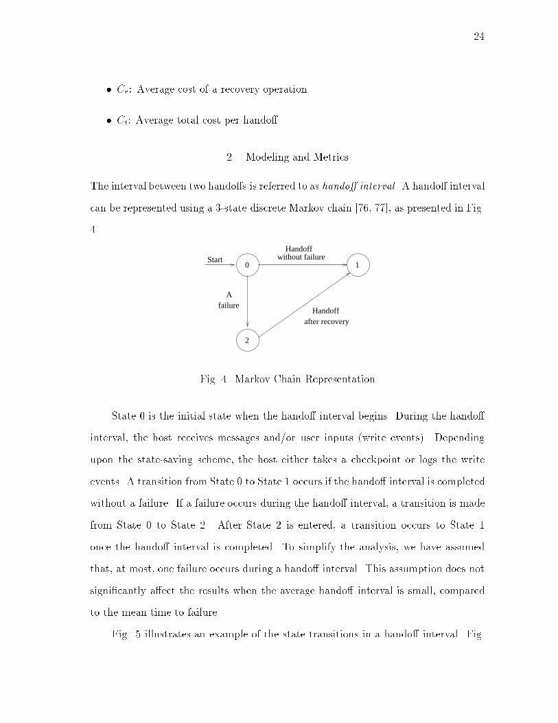
24� Cr: Average cost of a recovery operation.� Ct: Average total cost per hando�.2. Modeling and MetricsThe interval between two hando�s is referred to as hando� interval. A hando� intervalcan be represented using a 3-state discrete Markov chain [76, 77], as presented in Fig.4.0

2

1Start without failure

Handoff

Afailure

Handoffafter recoveryFig. 4. Markov Chain RepresentationState 0 is the initial state when the hando� interval begins. During the hando�interval, the host receives messages and/or user inputs (write events). Dependingupon the state-saving scheme, the host either takes a checkpoint or logs the writeevents. A transition from State 0 to State 1 occurs if the hando� interval is completedwithout a failure. If a failure occurs during the hando� interval, a transition is madefrom State 0 to State 2. After State 2 is entered, a transition occurs to State 1once the hando� interval is completed. To simplify the analysis, we have assumedthat, at most, one failure occurs during a hando� interval. This assumption does notsigni�cantly a�ect the results when the average hando� interval is small, comparedto the mean time to failure.Fig. 5 illustrates an example of the state transitions in a hando� interval. Fig.

255(a) is a case when the hando� interval is greater than a checkpoint interval. Thus,multiple checkpoint operations take place within a hando� interval. As seen in Fig.5(a), the initial state is state 0. A transition to state 2 takes place after a failure.State 2 begins with a recovery operation. A subsequent transition to state 1 takesplace after a hando� operation. Fig. 5(b) is a case when the checkpoint interval isgreater than a hando� interval. Thus, multiple hando� operations take place withina checkpoint interval. State transitions are similar to the previous case.T

Tc

Tc

T

X X

State 0

State 0State 2

State 1State 1State 2

Handoff Operation

Checkpoint Operation

Recovery Operation

X A Failure

State 0

State 1

(a) (b)Fig. 5. State IntervalsEach transition (a,b), from state a to state b in the Markov chain, has an as-sociated transition probability Pab and a cost Cab. Cost Cab of a transition (a,b) isthe expected total cost of operations that take place during the time spent in state abefore making the transition to state b.The transition probability P02 is the probability that a failure occurs within ahando� interval. Let tf be the time of failure, and th be the time of hando�. Then:P02 = P (tf < th) = Z 10 Z 1�f ��e���f e���h d�hd�f

26Solving the above, we get, P02 = ��+ �The expected duration from the beginning of the checkpoint interval until thetime when the failure occurred, given that a failure occurs before the end of thecheckpoint interval is,Tcexp = Z Tc0 t�e��t1� e��Tc dt = 1� � Tce��Tc1 � e��TcAs stated earlier,Nc(t) and Nl(t) denote the number of checkpoints and messageslogged in t time units, respectively. Cost C01 of transition (0,1) is the expected totalcost of operations that occur during the time spent in State 0 before making thetransition to State 1. C01 is as follows: (Recall that T is the mean hando� interval.)C01 = (�Cc) �Nc(T ) + (�Cl) �Nl(T ) + Ch (2:1)Performance metrics for the proposed schemes are:� Hando� Time: The hando� time is the additional time required to transfer thestate information from one base station to other, with the overhead of fault-tolerance.Basically it is the di�erence in the time duration of a hando� operation with faulttolerance and the time duration of a hando� operation without fault tolerance.� Recovery Cost: Upon a failure, this is the expected cost incurred by the recoveryscheme, to restore the host to the state just before the failure.� Total Cost: This is the expected cost incurred during a hando� interval with andwithout failure. The total cost is determined as follows:Ct = C01 + P02Cr (2:2)The costs will depend on the state-saving and hando� scheme used. We denote

27the total cost of a scheme that employs a combination of a state-saving scheme,X (X 2 fN;Lg), and a hando� scheme, Y (Y 2 fP;L; Tg) as CtXY .Now, we will derive the costs C01, Cr, and the hando� time for each scheme.The total cost Ct for each scheme can be determined by replacing the costs C01 andCr obtained, in (2.2). Our analysis assumes that the cost of transmitting a messagefrom one node to another depends on the number of hops between the two nodes.We also assume that neighboring base stations are at a distance of one network hopfrom each other. 3. No Logging-Pessimistic (NP) SchemeA checkpoint operation takes place upon every write event. Thus, upon every writeevent, the checkpoint is transferred over the wireless network to the base station,incurring a cost of �Cc, on average. There are r write events during a hando�interval. Since there is no logging operation involved, Nl(t) = 0; t � 0. During ahando�, the last checkpoint is transferred to the new base station, and in reply, anacknowledgement is sent. Therefore, the cost of hando� Ch = Cc + Cm. Thus:C01 = (r�+ 1)Cc + CmDuring recovery, the process state will be present at the current base station.Therefore, the recovery cost is the cost of transmitting a request message from themobile host to the base station, and the cost of transmitting the state over one hopof the wireless link. Thus: Cr = �(Cc + Cm)

284. No Logging-Lazy (NL) SchemeThe checkpoint and logging operations are similar to the NP scheme in Section D.3.However, upon the �rst checkpoint operation at the current base station, a controlmessage is sent to the base station that has the last checkpoint, requesting it to purgethat checkpoint. Let that base station be, on average, Nh hops from that current basestation. Thus, the average cost of purging is NhCm. A hando� operation includessetting a pointer at the current base station, and transferring a control messagebetween the current and the new base stations. Since setting a pointer does notinvolve any network usage, the cost of hando�, Ch, is equal to the cost, Cm, oftransferring a control message between the two base stations. Thus:C01 = r�Cc +NhCm + CmSince a checkpoint operation takes place upon every write event, and the check-point is not transferred to the new base station upon a hando�, the location of thelast checkpoint will depend on the number of hando�s since the last write event. Theupper bound on the number of hops traversed, to transfer the last checkpoint to thecurrent base station, will be the number of hando�s between two write events (or, inthis case, checkpoints). In addition to this, the cost of transferring the checkpointover the wireless link is incurred: �Cc. The average number of hando� operationscompleted since the last write event (or checkpoint event) until the time of failure isNh, where: Nh = �Tcexp (2:3)A cost is also incurred due to the request message from the mobile host for thecheckpoint. The cost is (�+Nh)Cm. Thus, an upper bound on the recovery cost isCr = (Nh + �)(Cc + Cm)

29We will use this Cr to evaluate CtNL. As this Cr estimated is an upper bound,CtNL estimated here is somewhat pessimistic.5. No Logging-Trickle (NT) SchemeThe checkpoint and logging operations are the same as for the NP and NL schemesdescribed in Sections D.3 and D.4. As in the NL scheme, the hando� cost is the costof transferring a control message from the current to the new base station. In additionto this, a control message is sent to the previous base station, requesting it to transferany state corresponding to the mobile host. This ensures that the maximum numberof hops traversed, to transfer the state during recovery, is one. The cost of the hando�operation is, thus, the sum of the cost of transferring the state over one hop of wirednetwork, and the cost of sending two control messages. Thus, Ch = Cc + 2Cm. Itshould be noted, however, that the hando� time is only determined by Cm, for thetransfer of a control message between the current and the new base station. The timespent due to the transfer of state is transparent to the user.Upon the �rst checkpoint operation at the current base station, a control messageis sent to the base station that has the last checkpoint, requesting it to purge thatcheckpoint. Let that base station be, on average, N 0h hops from the current basestation. Therefore, the cost of purging is N 0hCm. Thus:C01 = (r�+ 1)Cc + 2Cm +N 0hCmAs stated earlier, during the recovery operation, the number of hops traversedto transfer the state is, at most, one. Thus:Cr = (N 0h + �)(Cc + Cm) , where:N 0h = 1(1 � e��Tc) + 0(e��Tc) = (1 � e��Tc) , (2:4)

30where e��Tc is the probability that the last checkpoint took place at the current basestation. 6. Logging-Pessimistic (LP) SchemeFor this scheme, the state of the process will contain a checkpoint and a log of writeevents. The message log will contain the write events that have been processed sincethe last checkpoint. The logging cost will involve only those write events that have totraverse the wireless network to be logged at the base station. Only the user inputsneed to traverse the wireless network to be logged. On the other hand, write eventsreceived from other hosts in the network come via the base station anyway, so theyget logged �rst, and then forwarded to the mobile host. Thus, no cost is incurreddue to logging of write events from other hosts. As stated earlier, � is the fractionof write events that are user inputs. Thus, �r is the number of user inputs betweentwo hando�s. This is also the number of logging operations in a hando� interval. Foreach logging operation, there is a cost for the acknowledgment message sent by thebase station over the wireless network. The cost of each acknowledgment message is�Cm.The hando� cost will now include the cost of transferring the state as well asthe message log, and the cost of transferring an acknowledgment. Let � denote theaverage log size during hando�. Then, the average hando� cost will be (�Cl+Cc+Cm).Under the assumption of hando�s being a Poisson process, � = k�12 . (Recall that kis the number of write events per checkpoint.) Thus:C01 = r�Cck + �r�Cl + �r�Cm + �Cl + Cc + CmDuring recovery, the checkpoint and the log are present at the current basestation. Therefore, the recovery cost is the cost of transmitting a request message

31from the mobile host to the base station, and the cost of transmitting the checkpointand log over one hop of the wireless network. The expected size of the log at the timeof failure is � 0. For Poisson failure arrivals, �0 = k�12 . Therefore:Cr = �(�0Cl + Cc + Cm)7. Logging-Lazy (LL) SchemeThe checkpoint and logging operations are the same as for the LP scheme describedin Section D.6. When a checkpoint takes place, the old checkpoint and logs at thedi�erent base stations are purged. As also determined earlier in Section D.4, thepurging cost is NhCm, and the hando� cost is Cm.C01 = r�Cck + �r�Cl + �r�Cm +NhCm + CmAs determined earlier, the expected number of write events completed until thetime of failure since the last checkpoint is � 0 = k�12 . This is distributed over di�er-ent base stations. The last checkpoint and the logs have to traverse, on an average,Nh (2.3) hops on the wired network to reach the current base station, and an addi-tional wireless hop to reach the mobile host. A cost of (Nh + �)Cm is also incurreddue to the request message for the checkpoint and the logs (same as for NL scheme).Therefore, Cr = (Nh + �)(� 0Cl + Cc + Cm)8. Logging-Trickle (LT) SchemeThe checkpoint and logging operations are the same as in LP and LL. The cost ofhando� operation is, thus, the sum of the cost of sending two control messages (sameas for NT scheme), and the cost of transferring checkpoint and logs over one hop of

32wired network. Thus, Ch = �Cl + Cc + 2Cm. The cost of purging is N 0hCm. Thus:C01 = r�Cck + �r�Cl + �r�Cm + �Cl + Cc + 2Cm +N 0hCmCr = (N 0h + �)(� 0Cl + Cc + Cm)9. ResultsThe above equations have been normalized with respect to Cc. Recall that isthe relative logging cost and is equal to Cl=Cc. Thus, Cl = Cc. Recall that � is therelative control message cost and is equal to Cm=Cc. We assume that Cm � Cc (whichis the case, in practice). We replaceCc = 1, Cl = , and Cm = � in the above equationsand determine the hando� time, recovery cost and the total cost. The rate of writes� is set to 1.For our analysis, we assume that � = 0:5. (Recall that � is a fraction of writeevents that are user inputs.) This means that the write events comprise an equalpercentage of user inputs and messages from other hosts. For our analysis, we �x therelative control message cost, � = 10�4.a. Optimum Checkpoint IntervalAn optimum checkpoint interval is required to be determined only for the Loggingschemes. Recall that for a No Logging scheme, a checkpoint takes place upon everywrite event. However, for a Logging scheme, a checkpoint takes place periodicallyevery Tc units of time. Since the rate of writes � is equal to 1, the number of writeevents per checkpoint (k) is equal to Tc. A \good" value for k needs to be chosenfor the Logging schemes. We de�ne a good value of k to be the one that o�ers theminimum total cost. This value of k (say, koptLY , for a Logging scheme that usesscheme Y for hando�s: Y 2 fP;L; Tg) is a function of the failure rate �, relative

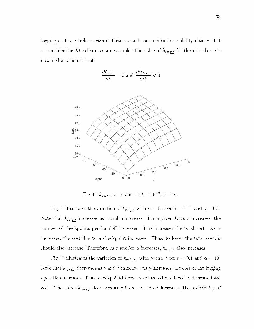
33logging cost , wireless network factor � and communication-mobility ratio r. Letus consider the LL scheme as an example. The value of koptLL for the LL scheme isobtained as a solution of: @CtLL@k = 0 and @2CtLL@2k < 00

0.20.4

0.60.8

1

0

20

40

60

80

10010

15

20

25

30

35

40

ralpha

kopt

Fig. 6. koptLL vs. r and �: � = 10�2, = 0:1Fig. 6 illustrates the variation of koptLL with r and � for � = 10�2 and = 0:1.Note that koptLL increases as r and � increase. For a given k, as r increases, thenumber of checkpoints per hando� increases. This increases the total cost. As �increases, the cost due to a checkpoint increases. Thus, to lower the total cost, kshould also increase. Therefore, as r and/or � increases, koptLL also increases.Fig. 7 illustrates the variation of koptLL, with and � for r = 0:1 and � = 10.Note that koptLL decreases as and � increase. As increases, the cost of the loggingoperation increases. Thus, checkpoint interval size has to be reduced to decrease totalcost. Therefore, koptLL decreases as increases. As � increases, the probability of

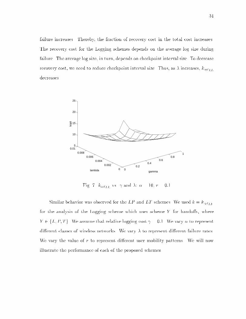
34failure increases. Thereby, the fraction of recovery cost in the total cost increases.The recovery cost for the Logging schemes depends on the average log size duringfailure. The average log size, in turn, depends on checkpoint interval size. To decreaserecovery cost, we need to reduce checkpoint interval size. Thus, as � increases, koptLLdecreases.0

0.20.4

0.60.8

1

0

0.002

0.004

0.006

0.008

0.015

10

15

20

25

gammalambda

kopt

Fig. 7. koptLL vs. and �: � = 10, r = 0:1Similar behavior was observed for the LP and LT schemes. We used k = koptLYfor the analysis of the Logging scheme which uses scheme Y for hando�s, whereY 2 fL;P; Tg. We assume that relative logging cost = 0:1. We vary � to representdi�erent classes of wireless networks. We vary � to represent di�erent failure rates.We vary the value of r to represent di�erent user mobility patterns. We will nowillustrate the performance of each of the proposed schemes.

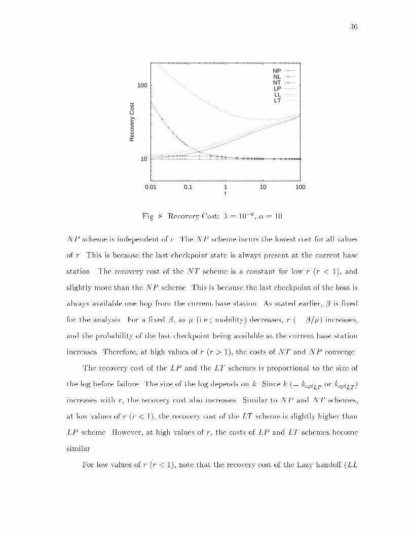
35b. Hando� TimeRecall that the hando� time is the additional time required, due to the transfer ofstate information by the fault tolerance scheme during hando� operation. Let BWbe the bandwidth of a link on the wired network. Table II illustrates the hando� costand (hando� time �BW ) of the various schemes. The Pessimistic hando� schemesincur a very high hando� time compared to the Lazy and Trickle hando� schemes.This is because in the Lazy scheme, there is no state transfer during hando�. In theTrickle scheme, the state transfer is performed separately from the hando�. Note,however, that for a given state-saving scheme, the hando� cost of the Trickle hando�scheme is almost equal to the Pessimistic hando� scheme.Table II. Hando� Cost and (Hando� Time �BW )Scheme Hando� Cost (Hando� Time �BW )NP 1 + � 1 + �NL � �NT 1 + 2� �LP 1 + � + � 1 + � + �LL � �LT 1 + 2�+ � �c. Recovery CostIn Fig. 8, we plot the recovery cost for all the schemes for � = 10, and � = 10�2.Similar behavior was observed for other values. As expected, the recovery cost ofthe Logging schemes is more than the No Logging schemes. The recovery cost of the

3610

100

0.01 0.1 1 10 100

Rec

over

y C

ost

r

NPNLNTLPLLLT

Fig. 8. Recovery Cost: � = 10�2, � = 10NP scheme is independent of r. The NP scheme incurs the lowest cost for all valuesof r. This is because the last checkpoint state is always present at the current basestation. The recovery cost of the NT scheme is a constant for low r (r < 1), andslightly more than the NP scheme. This is because the last checkpoint of the host isalways available one hop from the current base station. As stated earlier, � is �xedfor the analysis. For a �xed �, as � (i.e.; mobility) decreases, r (= �=�) increases,and the probability of the last checkpoint being available at the current base stationincreases. Therefore, at high values of r (r > 1), the costs of NT and NP converge.The recovery cost of the LP and the LT schemes is proportional to the size ofthe log before failure. The size of the log depends on k. Since k (= koptLP or koptLT )increases with r, the recovery cost also increases. Similar to NP and NT schemes,at low values of r (r < 1), the recovery cost of the LT scheme is slightly higher thanLP scheme. However, at high values of r, the costs of LP and LT schemes becomesimilar.For low values of r (r < 1), note that the recovery cost of the Lazy hando� (LL

37and NL) schemes are much larger than for the Pessimistic and the Trickle hando�schemes. This is because the checkpoint state might not be at the current base station.Secondly, the log of write events might be distributed at di�erent base stations. Thus,the cost of recovery will include the cost of transferring the checkpoint state and thelog from the various base stations to the current base station, and then forwardingthem to the mobile host over the wireless link. The LL scheme incurs a very highrecovery cost for low r. The lower the value of r, the greater the amount of scatter ofrecovery information. As r increases, the possibility of a checkpoint operation takingplace at the current base station increases. Thus, the recovery cost decreases as rincreases. However, as r increases, k (= koptLL) also increases. Thus, after some valueof r, the recovery cost starts increasing. On the other hand, the recovery cost of theNL scheme continues to decrease as r increases. At high values of r (r > 1), thecost of NL converges to NP and NT . Similarly, the cost of the LL scheme becomessimilar to LP and LT .As expected, at high values of r (i.e., low mobility), the recovery cost becomesalmost independent of the hando� scheme used { the state-saving scheme determiningthe recovery cost.d. Total CostFig. 9 illustrates the variation of total cost of various schemes with r, for � = 10�2and � = 10. The total cost is comprised of the failure-free cost and the recovery cost.The total cost of the Pessimistic hando� scheme and the Trickle hando� scheme arealmost equal (NP � NT , and, LP � LT ). The Lazy hando� scheme incurs a lowertotal cost at low values of r (r < 1). At high values of r, the total cost of the di�erenthando� schemes converge. However, the di�erence in the total costs of the Loggingand No Logging schemes remains. The total cost of No Logging scheme is higher than

380.01

0.1

1

10

100

1000

10000

0.01 0.1 1 10 100

Tot

al C

ost

r

NPNLNTLPLLLT

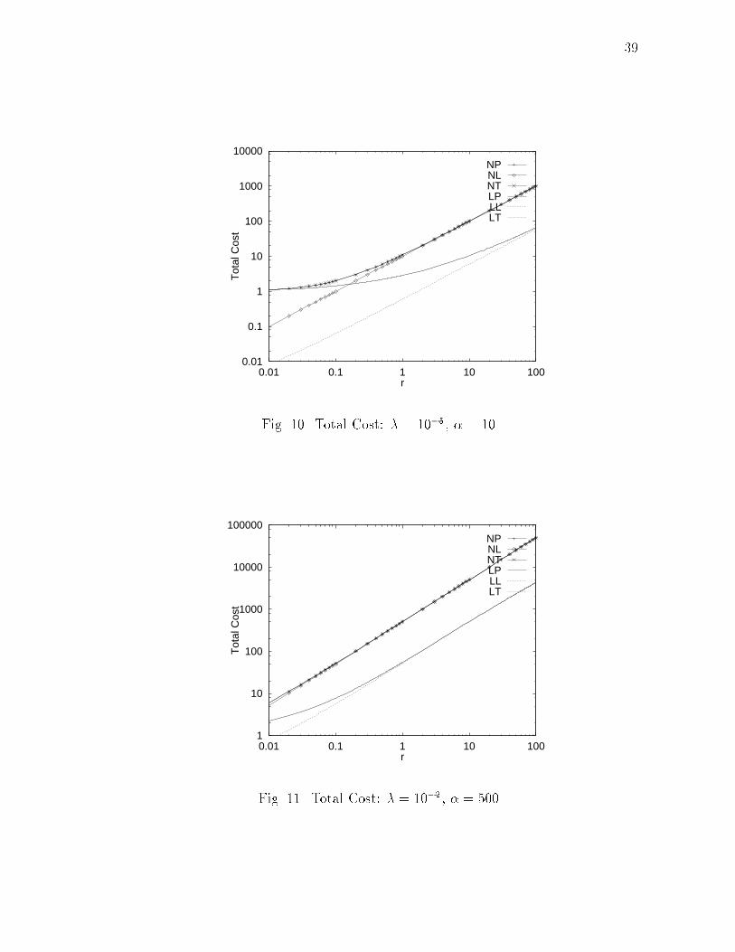
Fig. 9. Total Cost: � = 10�2, � = 10the Logging scheme for all values of r. The LL scheme incurs the lowest total costfor all r.Fig. 10 illustrates the variation of the total cost with r, for � = 10�5. Comparisonof Figures 9 and 10 indicates that, for the same �, as � decreases, the cost di�erencebetween the hando� schemes for the Logging state-saving scheme increases. As theprobability of failure decreases, the Lazy hando� scheme becomes more justi�ed. Thetotal costs of the Trickle and the Pessimistic hando� schemes are almost always equal,and both are higher than the Lazy scheme.Fig. 11 illustrates the variation of the total cost with r, for � = 500. The totalcost increases with �. Comparison of Figures 9 and 11 indicates that, for the same�, as � increases, the cost di�erence between the hando� schemes reduces. Thus, theperformance of a scheme becomes more dependent on the state-saving scheme usedthan on the hando� scheme.

390.01

0.1

1

10

100

1000

10000

0.01 0.1 1 10 100

Tot

al C

ost

r

NPNLNTLPLLLT

Fig. 10. Total Cost: � = 10�5, � = 101

10

100

1000

10000

100000

0.01 0.1 1 10 100

Tot

al C

ost

r

NPNLNTLPLLLT

Fig. 11. Total Cost: � = 10�2, � = 500

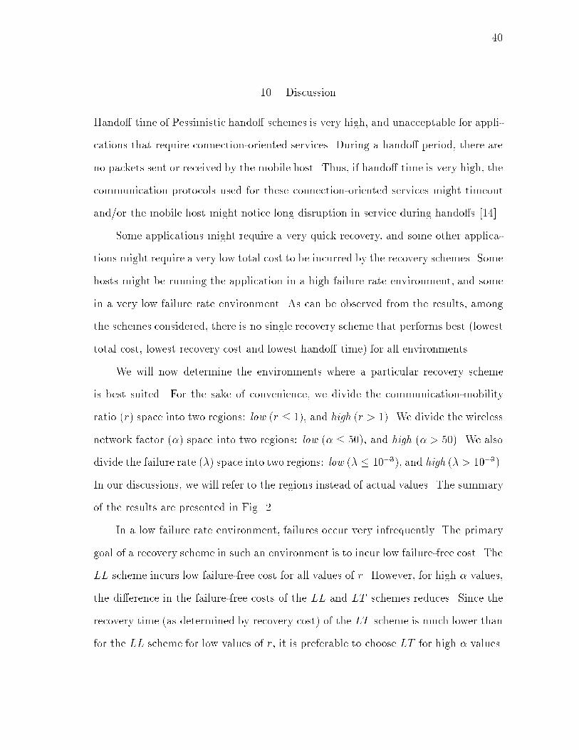
4010. DiscussionHando� time of Pessimistic hando� schemes is very high, and unacceptable for appli-cations that require connection-oriented services. During a hando� period, there areno packets sent or received by the mobile host. Thus, if hando� time is very high, thecommunication protocols used for these connection-oriented services might timeoutand/or the mobile host might notice long disruption in service during hando�s [14].Some applications might require a very quick recovery, and some other applica-tions might require a very low total cost to be incurred by the recovery schemes. Somehosts might be running the application in a high failure rate environment, and somein a very low failure rate environment. As can be observed from the results, amongthe schemes considered, there is no single recovery scheme that performs best (lowesttotal cost, lowest recovery cost and lowest hando� time) for all environments.We will now determine the environments where a particular recovery schemeis best suited. For the sake of convenience, we divide the communication-mobilityratio (r) space into two regions: low (r � 1), and high (r > 1). We divide the wirelessnetwork factor (�) space into two regions: low (� � 50), and high (� > 50). We alsodivide the failure rate (�) space into two regions: low (� � 10�3), and high (� > 10�3).In our discussions, we will refer to the regions instead of actual values. The summaryof the results are presented in Fig. 2.In a low failure rate environment, failures occur very infrequently. The primarygoal of a recovery scheme in such an environment is to incur low failure-free cost. TheLL scheme incurs low failure-free cost for all values of r. However, for high � values,the di�erence in the failure-free costs of the LL and LT schemes reduces. Since therecovery time (as determined by recovery cost) of the LT scheme is much lower thanfor the LL scheme for low values of r, it is preferable to choose LT for high � values.

41In a high failure rate environment, failures occur very frequently. The primarygoal of a recovery scheme is to incur low failure-free cost and low recovery cost. Forlow r values, the recovery cost of the LL and NL schemes is very high. Thus, weneed to choose between NT or LT . When � is low, NT incurs a low failure-freecost (slightly more than LT ), and provides a quicker recovery than LT . However,when � is high, LT becomes preferable. For high r values, LL is preferable over otherschemes.E. SummaryThe new mobile wireless environment presents many challenges due to the mobilenature of the hosts and the limited bandwidth on the wireless network. Presented inthis chapter are recovery schemes for a mobile wireless environment. The recoveryschemes are a combination of a state-saving strategy and a hando� strategy. Twostrategies for state-saving, namely, (i) No Logging and (ii) Logging, and three strate-gies for hando�, namely, (i) Pessimistic, (ii) Lazy, and (iii) Trickle are discussed.Our main goal here is to present the limitations of the new mobile computingenvironment, and its e�ects on recovery protocols. The trade-o� parameters to eval-uate the recovery scheme were identi�ed. It was determined that, in addition tothe failure rate of the host, the performance of a recovery scheme depended on themobility of the hosts and the wireless bandwidth. We analyzed the performance ofthe various recovery schemes proposed in this chapter, and determined those mobileenvironments where a particular recovery scheme is best-suited.

42CHAPTER IIICENTRALIZED LOCATION MANAGEMENTA. IntroductionIt is expected that existing wireless cellular networks will be upgraded for personalcommunication services (PCS) [20, 31, 58]. An important issue in mobile wirelessnetworks is the design and analysis of location management schemes. In order tocommunicate with any particular user, it is �rst necessary to locate the user in thenetwork. This is due to the fact that the users are mobile and they could be anywherein the area covered by the network.An analysis in [57] shows that if location updates are to occur on each cellcrossing the resulting signalling load will have a major impact on the load of thenetwork. The additional signalling tra�c on the SS7 signalling system (capacity of56 Kbps) is expected to be 4-11 times greater for cellular networks than for ISDN and3-4 times greater for future personal communication networks (PCN) than for cellularnetworks. The signalling load due to updates alone increases network load by 70%.Thus location updates will become a major bottleneck at the switches such as SS7,and hence mechanisms to control the cost of location update are needed. It is thusevident that new e�cient location management strategies need to be investigated forpersonal communication services (PCS).Location management consists of location searches and updates. A search occurswhen a host wants to communicate with a mobile host whose location is unknown tothe requesting host. An update occurs when a mobile host changes location.This chapter attempts to study the e�ect of forwarding pointers and search-updates on location management in Personal Communication Networks (PCN). Lo-

43cation management for PCS utilize the fact that there is a home location server (HLS)for every mobile host. There are existing standards for carrying out location manage-ment using home location servers (HLS), e.g., (EIA/TIA) Interim Standard 41 (IS-41), and Global System for Mobile Communications (GSM) in Europe [58]. However,these schemes are not e�cient, due to increase in network load and location manage-ment costs. To overcome these drawbacks, this chapter presents location managementstrategies using forwarding pointers in addition to HLS. We present two heuristics tolimit the number of forwarding pointers traversed during a search, namely,movement-based and search-based. We show that signi�cant improvement can be obtained usingforwarding pointers in addition to HLS. The chapter also presents a strategy toperform search-updates. A search-update occurs after a successful search, when thelocation information corresponding to the searched mobile host is updated at somehosts. Analysis shows that performing search-updates signi�cantly reduces the searchcosts. However, search-updates also increase the total network load. This extra net-work load is due to forwarding pointer maintenance.The performance of the proposed heuristics depend on (i) the relative cost ofsetting and traversing the forwarding pointers (parameter �), and, (ii) call and mo-bility patterns of the user (parameter r). Through analysis, we show that among theschemes considered, there is no single location management scheme that performswell for all values of r and �. However, among the schemes considered, we determinethe best location management scheme for each environment, as shown in Fig. 12.M is a parameter that determines the performance of the movement-based heuristicscheme. It will be explained in detail in Section D.2.b.On the downside, forwarding pointers are prone to failures anywhere along thechain of pointers. Omission/corruption of a forwarding pointer could cause the hostto be intractable. This chapter proposes cost-e�ective techniques for fault tolerance

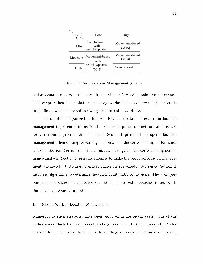
44r

α

Low

High

Search-basedwith

Moderate

(M<5)

Movement-

Search-Updates

based

Movement-based(M<3)

Search-based

Low High

Movement-basedwith

Search-Updates

(M<5)Fig. 12. Best Location Management Schemeand automatic recovery of the network, and also for forwarding pointer maintenance.This chapter then shows that the memory overhead due to forwarding pointers isinsigni�cant when compared to savings in terms of network load.This chapter is organized as follows. Review of related literature in locationmanagement is presented in Section B. Section C presents a network architecturefor a distributed system with mobile hosts. Section D presents the proposed locationmanagement scheme using forwarding pointers, and the corresponding performanceanalysis. Section E presents the search-update strategy and the corresponding perfor-mance analysis. Section F presents schemes to make the proposed location manage-ment scheme robust. Memory overhead analysis is presented in Section G. Section Hdiscusses algorithms to determine the call-mobility ratio of the users. The work pre-sented in this chapter is compared with other centralized approaches in Section I.Summary is presented in Section J.B. Related Work in Location ManagementNumerous location strategies have been proposed in the recent years. One of theearlier works which dealt with object tracking was done in 1986 by Fowler [21]. Fowlerdeals with techniques to e�ciently use forwarding addresses for �nding decentralized

45objects. Our research borrows the idea of manipulating forwarding pointers upon asuccessful search.Awerbuch et.al. proposed a theoretical model for online tracking of mobilehosts [4]. Their architecture consists of a hierarchy of \m-regional matching directo-ries". In their scheme, forwarding pointers and regional matching directories are usedto enable localized updates and searches.Spreitzer et.al. proposed a network architecture which consists of user agentsand a location query service (LQS) [72]. There is a dedicated user agent per userand these user agents are responsible to forward any communication to or from theuser. This scheme is mainly aimed for local networks { the kind used within buildingpremises. As the number of hosts in a network increase, it might not be e�cient tohave a dedicated user agent per user.Wu et. al. dealt with the idea of caching location data at the Internet AccessPoint(IAP ) [79]. Here, the IAP will maintain location data of some of the hosts. Thisbecomes useful when optimal routing decisions are to be taken. If the IAP does nothave an entry for a host, the message is forwarded to the Mobile Router (MR) whichmaintains information of all the hosts. It is a very simple idea that will be e�ectivefor local networks. However, when the network sizes increase, the MR will becomea serious bottleneck, and one has to resort to more e�cient location managementtechniques.Ioannidis et.al. proposed IP-based protocols for providing continuous networksaccess for mobile computers using caching and forwarding technique [32]. However,these protocols are primarily proposed for a campus environment with mobile com-puters.Badrinath et.al. examine strategies that reduce search costs and control thevolume of location updates by employing user pro�les [5]. Their architecture consists

46of a hierarchy of location servers which are connected to themselves and to the basestations (or mobile support stations) by a static network. User pro�les are used tocreate partitions. It is only when the user crosses partitions that the update takesplace. However, in most cases, user pro�les are not always available a priori.A modi�ed tree structure for location management was proposed in [19]. Theroot and the some of the higher levels of the tree was replaced by a set-ary butter ynetwork. This helped in balancing the search requests at the nodes. Also proposedwere schemes to make the protocol self-stabilizing.The idea of location management with home location servers (HLS) has alsobeen proposed in [36, 37]. Caching [36] and forwarding [37] have been independentlyproposed for Personal Communication Services (PCS). Similar to our work in thischapter, these strategies augment the basic location strategy which uses HLS. Sec-tion I compares them with the work presented in this chapter. Other techniques likeuser pro�le replication [71] and local anchoring [29] have also been proposed to reducenetwork load due to location management. In the next section we will present thenetwork architecture typically used in centralized location management schemes.C. Network ArchitectureCells are grouped into registration areas. There is a location server in each registrationarea. Each mobile host is assumed to be permanently registered to a particularregistration area. The location server of that registration area is called the homelocation server (HLS) for the mobile host. This association of a host with a particularhome location server is fully replicated across the whole network. The home locationserver is responsible for keeping track of the location information of the mobile host.A location server is also responsible for maintaining location information of the mobile

47hosts currently residing (visitors) in all cells within its registration area1.The events that can cause change in the location information of a mobile hostare when the mobile host (i) Switches ON, (ii) Switches OFF, (iii) Hando�s, and (iv)Crosses registration areas. The details of the events (i), (ii) and (iii) are discussedin Appendix A. In this research we are primarily interested in analysing strategiesfor location management due to registration area crossings, because these strategiesinvolve updates at the home location servers and thus increasing the network tra�c.In the next section we will discuss the location management strategies for registrationarea crossings.D. Location ManagementIn this section, we �rst present the scheme for updates and searches that is beingcurrently used in IS-41. We will then present the drawbacks of these schemes. Laterin this section we will present the proposed location management scheme using for-warding pointers, and the corresponding performance analysis.1. Overview of the Basic IS-41 SchemeLocation management with home location servers is being used in current personalcommunication systems (PCS) standards proposals such as IS-41 [58].1The terminology used in IS-41 literature is slightly di�erent. IS-41 uses homelocation register (HLR) and visitor location register (V LR) databases. However,the information maintained in the HLR is same as what is maintained in HLS, theinformation maintained in the V LR is maintained in the various location servers.

48id LS

id MSSnew_lsold_ls

1

mh

new_mss

mh new_mss

mh new_ls

HLS

2

id HLS

mh HLS

3

4

5

6

78

9

10

Fig. 13. Update in the Basic Scheme (IS-41)a. Updates in the Basic IS-41 SchemeUpdates take place only when the mobile host (mh) enters a new registration area.Let the old registration area be old, and the new registration area be new. Please referFig. 13 for this discussion. Upon entering new, the mobile host (mh) informs the newmobile support station (new mss), which forwards the information to the locationserver of registration area new, named new ls (steps 1-2 in Fig. 13). The new lslooks up its database to determine the home location server (HLS) of mh (step 3).The new ls then sends a message to HLS notifying it about the new location ofmh (step 4). The HLS updates the location information of mh (i.e., changes thecurrent location server to new ls), and sends the host information (user pro�le, etc.)to new ls (steps 5-6). The location server new ls stores the user pro�les, updatesits host database and sends an acknowledgement to new mss (steps 7-8). The HLS

49src_mss

src_ls dest_ls

dest_HLS

1

2

src

dest dest_HLSid HLS

id LS

dest dest_ls

id MSS

dest dest_mss

3 4

5

6

7

89

10Fig. 14. Search in the Basic Scheme (IS-41)also sends a message to the location server of registration area old, named old ls,requesting it to delete any host information stored at old ls (step 9). The locationinformation of the mobile host is then purged from old ls, after that, old ls sends acon�rmation message to HLS (step 10).b. Searches in the Basic IS-41 SchemeLet us suppose that a mobile host src wants to communicate with another mobilehost dest. Let src mss be the MSS of the cell in which host src currently resides.When src wants to communicate with a mobile host dest, it has to �rst determinethe location of dest. Host src sends a location query message to the mobile supportstation for its cell, src mss (step 1 in Fig. 14). The src mss, forwards the query tothe location server (say src ls) in its registration area (step 2 in Fig. 14). The locationserver src ls checks whether dest is in its registration area2. If dest is in its registration2In IS-41 standard, every call results in a query to the HLS of dest. In this chapterwe have altered the search procedure slightly to search the registration area of thecaller �rst. Thus, the search procedure of IS-41 standard will in fact result in an even

50area, then it returns the location information. Otherwise, src ls looks up its databaseto determine the HLS of dest (say dest HLS) (step 3). The location server src lsthen forwards the location query message to dest HLS (step 4). The dest HLSmaintains the identi�cation of the location server (say dest ls) of the registrationarea in which the last update of the location of host dest took place (step 5). Thedest HLS queries the dest ls for the cell location of dest (step 6). In reply, dest lssends the identi�er of the mobile support station dest mss. Upon getting the replyfrom dest ls (steps 7 and 8), dest HLS returns the current location of dest to src ls,which, in turn forwards it to src mss (steps 9 and 10). The location informationis nothing but the address of the MSS (named dest mss) of the cell in which themobile host dest currently resides. Thereafter, the call is set up between src and destvia src mss and dest mss.c. Drawbacks� Increase in network tra�c when the host crosses registration areas very fre-quently: This can be due to a very mobile host going in some speci�c direction,or because the host moves in and out of a registration area such that there arelot of registration area boundary crossings. As every registration area crossingcauses an update at the host's HLS, this scheme increases the network tra�c.� Ine�cient location management: Updates on each registration area crossing isuseful to reduce the search costs (i.e., call set-up time), only if the user is beingcalled frequently. However, if the user is not being called frequently, updateson each crossing are not necessary. In such scenarios, updates on each crossinglead to ine�cient location management.higher network load than the search procedure presented here.

512. Proposed SchemeIn this section we will discuss the proposed scheme that tries to avoid the drawbacksof the above location management strategy. We use forwarding pointers in additionof HLS to assist in location management. Our main goal is to avoid the increasein network tra�c due to updates at the HLS. We achieve this by not updatingthe location information after every registration area crossing. Instead, forwardingpointers are maintained at the location servers of the registration areas visited asdescribed below.We classify location updates further into two types, namely, updates and search-updates. A update occurs when a mobile host changes location. A search-update (alsoknown as caching [36]) occurs after a successful search, when some hosts update thelocation information corresponding to the searched mobile host. We discuss moreabout search-updates in Section E.a. Forwarding PointersA forwarding pointer maintained at some location server for a mobile host mh is adata structure that contains the following: (i) identi�er of mh, (ii) location of thehost mh. The key for the forwarding pointer database is the identi�er of mh, i.e.,there can be only one forwarding pointer per mobile host.The forwarding pointers for a mobile host can be interpreted as forming a directedgraph with the location servers as vertices and with an edge from location server ls1to location server ls2 if and only if ls1 has a forwarding pointer that points to ls2.The resulting graph will be a tree with edges directed towards the root, the currentlocation of the mobile host [21].Example D.1: For an easier understanding we will illustrate with an example. Let

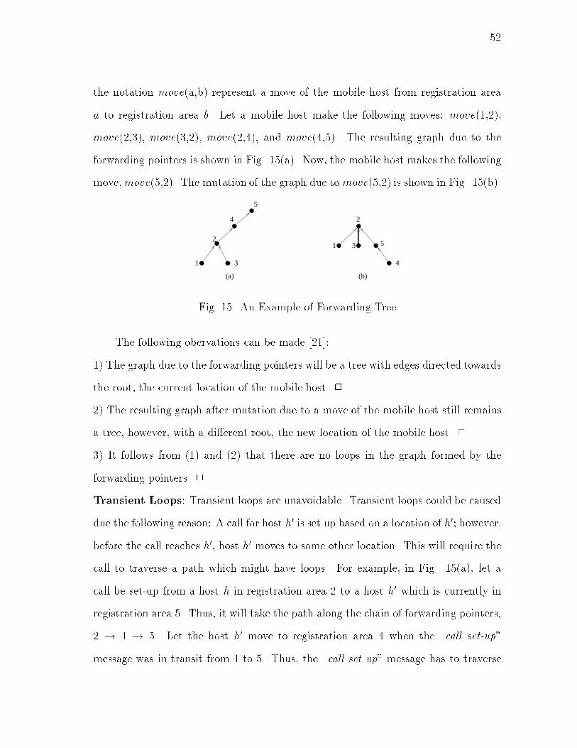
52the notation move(a,b) represent a move of the mobile host from registration areaa to registration area b. Let a mobile host make the following moves: move(1,2),move(2,3), move(3,2), move(2,4), and move(4,5). The resulting graph due to theforwarding pointers is shown in Fig. 15(a). Now, the mobile host makes the followingmove,move(5,2). The mutation of the graph due to move(5,2) is shown in Fig. 15(b).(a) (b)

1 3

2

4

5

1 3 5

2

4Fig. 15. An Example of Forwarding TreeThe following obervations can be made [21]:1) The graph due to the forwarding pointers will be a tree with edges directed towardsthe root, the current location of the mobile host. 22) The resulting graph after mutation due to a move of the mobile host still remainsa tree, however, with a di�erent root, the new location of the mobile host. 23) It follows from (1) and (2) that there are no loops in the graph formed by theforwarding pointers. 2Transient Loops: Transient loops are unavoidable. Transient loops could be causeddue the following reason: A call for host h0 is set up based on a location of h0; however,before the call reaches h0, host h0 moves to some other location. This will require thecall to traverse a path which might have loops. For example, in Fig. 15(a), let acall be set-up from a host h in registration area 2 to a host h0 which is currently inregistration area 5. Thus, it will take the path along the chain of forwarding pointers,2 ! 4 ! 5. Let the host h0 move to registration area 4 when the \call set-up"message was in transit from 4 to 5. Thus, the \call set up" message has to traverse

53the forwarding pointer 5 ! 4, thereby visiting registration area 4 twice. However,these loops are short-lived, and do not exist under stable conditions.b. Updates Using Forwarding PointersWhenever a mobile host leaves a registration area, say old, and enters a new regis-tration area, say new, the host information (e.g., user pro�le, number of forwardingpointers created due to the moves, etc.) is transferred from old ls to new ls, where,old ls (new ls) is the location server for old (new) registration area. In addition, aforwarding pointer is created at old ls to point to new ls to indicate that the hosthas moved to new.Update at the HLS does not take place for every registration area crossing.When an update takes place is determined using one of the heuristics stated below:� Movement-based heuristic: The location information of a host at the HLS isupdated when the number of registration area crossing by the host isM, whereM is a constant parameter that determines the performance of this heuristic.� Search-based heuristic: The location information of a host at the HLS isupdated when the number of search requests for the host is S, where S is aconstant parameter that determines the performance of this heuristic.The procedure to update the HLS in the proposed scheme is same as the updateprocedure in Section D.1.a. After such an update, the HLS will know the presentlocation of the mobile host, and no forwarding pointers need to be traversed (untilthe mobile host moves from its present registration area).

54src_mss

src_ls

dest_HLS

1

2

src

dest dest_HLSid HLS

id LS

dest dest_ls

dest_ls ls1 curr_ls

id

dest

Forw.ptr

ls1

id

dest

Forw.ptr

next_ls

id

dest dest_mss

MSS

3 4

5

6

8 10

7 9 11

i

i+1Fig. 16. Search using HLS and Forwarding Pointersc. Location Searches Using Forwarding PointersLet us suppose that a mobile host src wants to communicate with another mobilehost dest. Please refer Fig. 16 for this discussion. The �rst four steps of the searchprocedure are identical to steps 1-4 in Fig. 14, until the location query is forwardedto the home location server of dest, dest HLS. Dest HLS returns the address of thelocation server (dest ls) of the registration area in which the mobile host was residingwhen the last update at dest HLS took place (steps 5 and 6). Upon receiving theaddress of dest ls, src ls sends a message query that traverses the chain of forwardingpointers originating at dest ls (step 7). Each location server on the chain looks up itsforwarding pointer database to determine the next location server on the chain, andforwards the location query to it (e.g., steps 8 and 9 for dest ls). This continues tillthe end of the chain is reached (say curr ls is the location server). The host dest willbe located in a cell in the registration area of curr ls. The location server curr lsreturns the current cell location to src ls, which in turn forwards it to src mss (stepsi and i + 1 in Fig. 16). Thereafter, the call is set up between src and dest via the

55src mss and dest mss.d. Forwarding Pointer MaintenanceForwarding pointers for a host may remain at the location servers for a long timecontaining stale information and also increasing the storage requirements at the loca-tion servers. A forwarding pointer can potentially be purged if it has not been usedfor a \long" time. To avoid any inconsistencies in the location information due topurging, we require the location servers to maintain a timestamp associated with eachforwarding pointer. While creating a forwarding pointer, the timestamp is the currenttime at the location server when the pointer is created. Along with the timestamp,the purge time interval tp for that pointer is also maintained. Every location serverpurges the forwarding pointers which are older than purge time interval tp units oftime. Through this process, we avoid maintaining any stale forwarding pointers atthe location servers.A Note: The above data structure contains a �eld to store time. The time entryfor a data structure on a location server, say ls, contains the local time at locationserver ls when the data structure was last modi�ed. It should be noted that thecorrectness of the algorithms does not require the clocks at various location serversto be tightly synchronized.However, there might be \dangling" pointers due to inconsistent purging. Forexample, let there be a chain 5 ! 4 ! 2. Thus, the current location of the host is2. Suppose, 4 purges its pointer to 2 before 5 purges its pointer to 4. Then, 5! 4 isa \dangling" pointer because it does not lead to the location of the host i.e., 2. Toavoid this, a trivial solution is to keep a constant value of tp for all pointers3. Let3This requires that clocks of all the location servers progress at an identical rate.

56it be Tpurge. Let us consider the example again. Since, the pointer 4 ! 2 is createdafter pointer 5 ! 4, the pointer 5 ! 4 will be purged before pointer 4 ! 2. Thus,there will not be any \dangling" pointers.We also need to ensure that the forwarding pointers do not get purged before anHLS update takes place. Thus, the mobile host should update its location informa-tion at its HLS at least once every Tpurge units of time. This will ensure that evenif the forwarding pointers are purged, the HLS has the current location informationof the host. Tpurge will be a system design parameter. Larger the value of Tpurge,lower will be the volume of HLS updates due to purging. However, larger the valueof Tpurge, longer will the forwarding pointers be in the system, thus increasing thestorage requirements at the location server. In a later section we derive the relationbetween Tpurge and the memory overhead at the location servers.In the analysis presented in the next section, we assume that Tpurge is large enough(as compared to the time period between two HLS updates due to heuristics) suchthat HLS updates due to timeout form a small fraction of all HLS updates. So, wewill ignore those cases. We now analyze the performance of the search-based heuristicand the movement-based heuristic.3. Performance AnalysisIn this section we analyze the proposed location management scheme using forwardingpointers and compare it with the basic scheme (IS-41). We will then compare theThis may not be valid in practice, because, the clocks will have di�erent rates. How-ever, we can tackle this by having di�erent purge time intervals for the locationservers. The di�erence between the purge time intervals at any two location serverswill mainly depend on the relative clock rate of the two location servers. For sim-plicity of explanation we assume that clocks at all the location servers progress at anidentical rate.

57performance of the two heuristics presented in this chapter.Calls between two hosts within the same registration area will not involve thehome location servers. Moves within the registration area will also not involve anyhome location server interaction. Therefore, we analyze the performance of the lo-cation management schemes for calls which arrive from outside the registration areaof a host (hereafter, we refer them simply as call arrivals), and for moves which areregistration area crossings. We de�ne \cost" of sending a message as the amount ofnetwork usage due to sending the message. In other words, it is the amount of timethe network is busy trasmitting the message.The following terminology is used in the analysis:� r = average number of calls per registration area crossing. We call this thecall-mobility ratio.� Cu = cost of an update per registration area crossing using IS-41. We will derivean expression for Cu later.� Cs = cost of a location search using IS-41. We will derive an expression for Csbelow.� C 0u; C 0s are the update and search cost, respectively, using forwarding pointers.� cost(x! y) = cost of sending a message from x to y.� A = average cost of sending a location query/reply message betweenMSS andthe LS within a registration area.� B = average cost of sending a location query/reply message between a locationserver and a home location server. This is thus the average cost of a HLSinteraction.

58� k = For a caller host, this is the number of forwarding pointers traversed beforelocating the destination host.� F = cost of setting a forwarding pointer between two location servers. Thiscost includes the cost of sending a message between the two location servers.The cost of traversing a forwarding pointer also includes the cost of sendinga message between two location servers. The cost of traversing a forwardingpointer is also assumed to be F .� � = Relative forwarding cost = FCu .In this chapter, our goal is to analyze the load on the static network. Therefore,we do not consider the cost of message transfers over wireless links.a. Performance MetricsThe performance metrics of the schemes are search cost (Cs), and total cost (Ct)where, Ct = XCu + YCsWe need to choose X and Y such that the following holds:� For users with low r (i.e., moves are more frequent than calls received), theupdate cost is the governing factor in the total cost. Thus, in this case, thesearch cost should be dampened.� For users with high r (i.e., calls received are more frequent than moves), thesearch cost is the governing factor in the total cost. In this case, the updatecost should be dampened.

59To achieve the above, we choose X = 1r , and Y = r. Thus, the performance metricof the schemes is: Ct = 1rCu + rCsLet, Ct (= 1rCu+rCs) be the total cost for the IS-41 scheme, and C 0t (= 1rC 0u+rC 0s)be the total cost for the proposed scheme using forwarding pointers. For the proposedscheme to perform better than the IS-41 scheme, we require the following conditionsto be true:� Condition 1: C 0t � Ct, and� Condition 2: C 0s � RCs.If the proposed scheme satis�es both the conditions, the network load will bereduced without considerably increasing the call set-up time for the user. The valueof R will depend on the quality of service of requirements of the user. We chooseR = 2.For the sake of convenience, we divide the r space into three regions: low (r <0:1), moderate (0:1 � r < 5) and high (r � 5). We also divide the � space into tworegions: low (� < 0:5), and high (� � 0:5). In our discussions, we will refer to theregions instead of actual values.b. IS-41 SchemeLet a mobile host mh move from a registration area to a new registration area, and,let the corresponding location servers be old ls and new ls respectively. Let the newmobile support station be new mss. Let the home location server of mh be HLS.From the update scheme presented in Section D.1.a, and Fig. 13 we can obtain,Cu = cost(new mss! new ls) + cost(new ls! HLS) + cost(HLS ! new ls)+cost(new ls! new mss) + cost(HLS ! old ls) + cost(old ls! HLS)

60= A+B +B +A+B +B= 2A+ 4BStep 1 involves message transfer over the wireless link, and hence is not considered inthe cost analysis. Steps 3 and 5 in Fig. 13 are database lookup and update operations,and do not incur any network load. Thus, they too are not considered in the costanalysis.Let a mobile host src call another mobile host dest. Let the location servers ofthe registration areas in which src and dest are currently residing be src ls and dest lsrespectively. Let the home location server of dest be dest HLS. From Section D.1.band Fig. 14, we can obtain,Cs = cost(src mss! src ls) + cost(src ls! dest HLS)+cost(dest HLS ! dest ls) + cost(dest ls! dest HLS)+cost(HLS ! src ls) + cost(src ls! src mss)= A+B +B +B +B +A= 2A+ 4B (3.1)Step 1, 3, 5, 7 do not incur any network load. Thus, they are also not considered inthe cost analysis.c. Movement-based HeuristicAs stated earlier, the number of registration areas crossed by a host when the movement-based heuristic scheme performs an update for that host is M. Thus, the number offorwarding pointers due to moves by the host when an update takes place for thathost is (M� 1). Since the number of forwarding pointers for a host when an updatetakes place is (M� 1), (M� 1)F is the total cost of creating forwarding pointers

61before an update takes place for that host. Therefore the update cost per registrationarea crossing for the movement-based heuristic scheme is,C 0u = 1M((M� 1)F + Cu)From Fig. 16 we can obtain the search cost for the movement-based scheme as follows:C 0s = cost(src mss! src ls) + cost(src ls! dest HLS)+cost(dest HLS ! src ls) + cost(traversing theforwarding pointers to curr ls) + cost(curr ls! src ls)+cost(src ls! src mss)Step 1 in Fig. 16 involves message transfer over the wireless link, and hence is notconsidered in the cost analysis.We make a conservative estimate of the cost (curr ls ! src ls). In the worstcase, this cost will be equal to kF (the cost of traversing the forwarding pointers).Therefore, C 0s = A+B +B + kF + kF +A= 2A+ 2B + 2kF (3.2)From equations (3.1) and (3.2), we get,C 0s = A+ Cs2 + 2kFThe average value of k is upper bounded by (M� 1)=2. Thus, the average searchcost is as follows: C 0s = A+ Cs2 + (M� 1)FWe will now determine the relative total cost (C 0t=Ct) and relative search cost (C 0s=Cs).

62The relative total cost is given as follows:C 0tCt = 1rC 0u + rC 0s1rCu + rCs= 1rM(Cu + (M� 1)F ) + r(A+ 12(Cs + 2(M� 1)F ))1rCu + rCs (3.3)We assume that the cost B of HLS interactions is the dominant cost in Cs and Cu.This may not be true for all network architectures. This assumption was mainlymotivated by the studies which indicate HLS to be the bottleneck in PCNs. Theforwarding cost F is assumed to be a fraction of the cost of update and searches, i.e.,F = �Cu, where, � � 1. Substituting F = �Cu, A � Cu, and Cs = Cu in (3.3)yields, C 0tCt = 12M (1 +Mr2)(1 + 2�(M� 1)) + 11 + r2 ! (3:4)The relative search cost is given as follows:C 0sCs = 12(1 + 2�(M� 1)) (3:5)Using the above equations we will now determine the values of M that satis�esthe conditions stated in Section D.3.a. Condition 2 requires the search cost of theproposed scheme to be less than or equal to twice than the search cost of the IS-41scheme. For this condition to be satisi�ed, following should hold:M� 3 + 2�2�Fig. 17 illustrates the variation of maximum allowable M with �. Note, that forlow � values,M > 5 is allowable. Figs. 18-20 illustrate the variation of relative totalcost with r for di�erent values of M, for � = 0:2; 0:5 and 0:8 respectively. It can beobserved that at high values of r, Condition 1 is violated for high values of M. Inother words, long chain lengths are not suitable at high values of r. Thus, a small

632

4

6

8

10

12

14

16

0.1 0.2 0.3 0.4 0.5 0.6 0.7 0.8 0.9 1

Max

imum

M

Alpha

M

Fig. 17. Maximum Allowable Chain LengthM has to be chosen in order to obtain good performance for a wide range of r and�. We keepM < 5 in our analysis. We analyze the performance of movement-basedheuristic scheme for M = 2, 3 and 4. Note that in Figs. 18-20, the relative totalcost of the movement-based scheme increases as r and � increases. Longer chainlengths (i.e., larger M) are preferred at low values of r. However, as r increases,schemes using smaller chain lengths (smaller M) perform better. It can be seen inFig. 19 and Fig. 20 that for high � values, the performance of movement-basedheuristic with large M performs worse than the IS-41 scheme at high values of r.Figs. 21-23 illustrate the variation of the relative search cost of the movement-based heuristic scheme with r for � = 0:2; 0:5 and 0:8 respectively. It can be observedthat the relative search cost of the movement-based heuristic scheme is independent ofr. However, the relative search cost increases with �. At high values of �, Condition2 is violated for large values M.Thus, it is recommended that the chain lengths be kept small (< 5). This isbecause, schemes with long chain lengths perform poorly in terms of search cost as

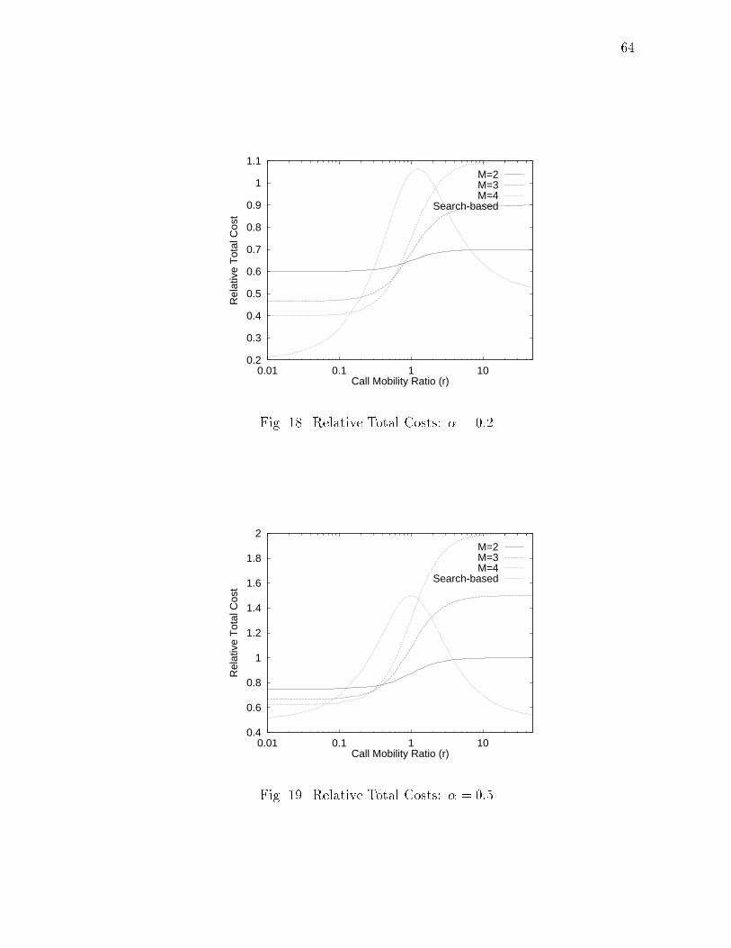
640.2

0.3

0.4

0.5

0.6

0.7

0.8

0.9

1

1.1

0.01 0.1 1 10

Rel

ativ

e T

otal

Cos

t

Call Mobility Ratio (r)

M=2M=3M=4

Search-based

Fig. 18. Relative Total Costs: � = 0:20.4

0.6

0.8

1

1.2

1.4

1.6

1.8

2

0.01 0.1 1 10

Rel

ativ

e T

otal

Cos

t

Call Mobility Ratio (r)

M=2M=3M=4

Search-based

Fig. 19. Relative Total Costs: � = 0:5

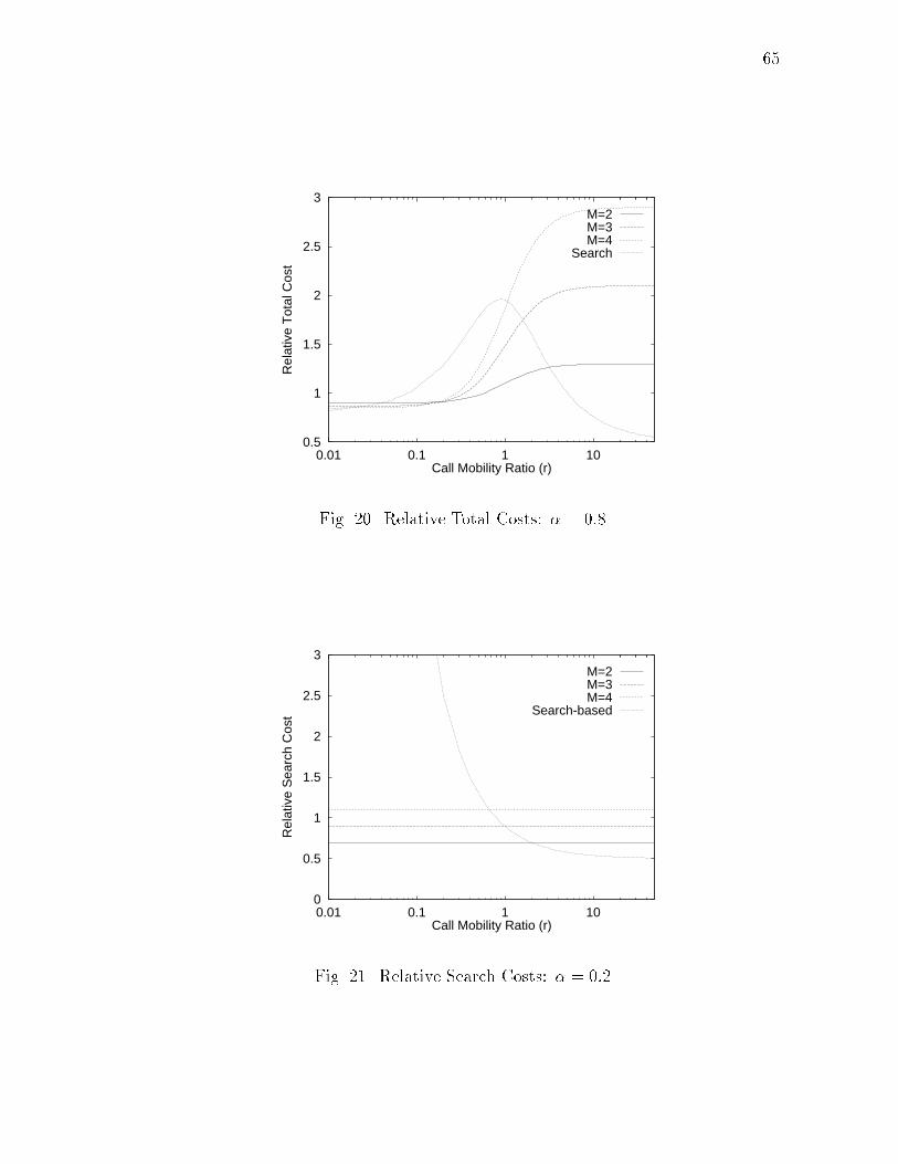
650.5

1

1.5

2

2.5

3

0.01 0.1 1 10

Rel

ativ

e T

otal

Cos

t

Call Mobility Ratio (r)

M=2M=3M=4

Search

Fig. 20. Relative Total Costs: � = 0:80

0.5

1

1.5

2

2.5

3

0.01 0.1 1 10

Rel

ativ

e S

earc

h C

ost

Call Mobility Ratio (r)

M=2M=3M=4

Search-based

Fig. 21. Relative Search Costs: � = 0:2

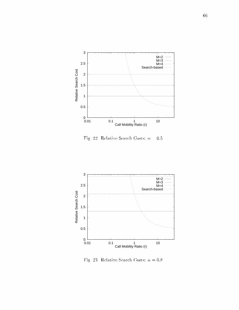
660

0.5

1

1.5

2

2.5

3

0.01 0.1 1 10

Rel

ativ

e S

earc

h C

ost

Call Mobility Ratio (r)

M=2M=3M=4

Search-based

Fig. 22. Relative Search Costs: � = 0:50

0.5

1

1.5

2

2.5

3

0.01 0.1 1 10

Rel

ativ

e S

earc

h C

ost

Call Mobility Ratio (r)

M=2M=3M=4

Search-based

Fig. 23. Relative Search Costs: � = 0:8

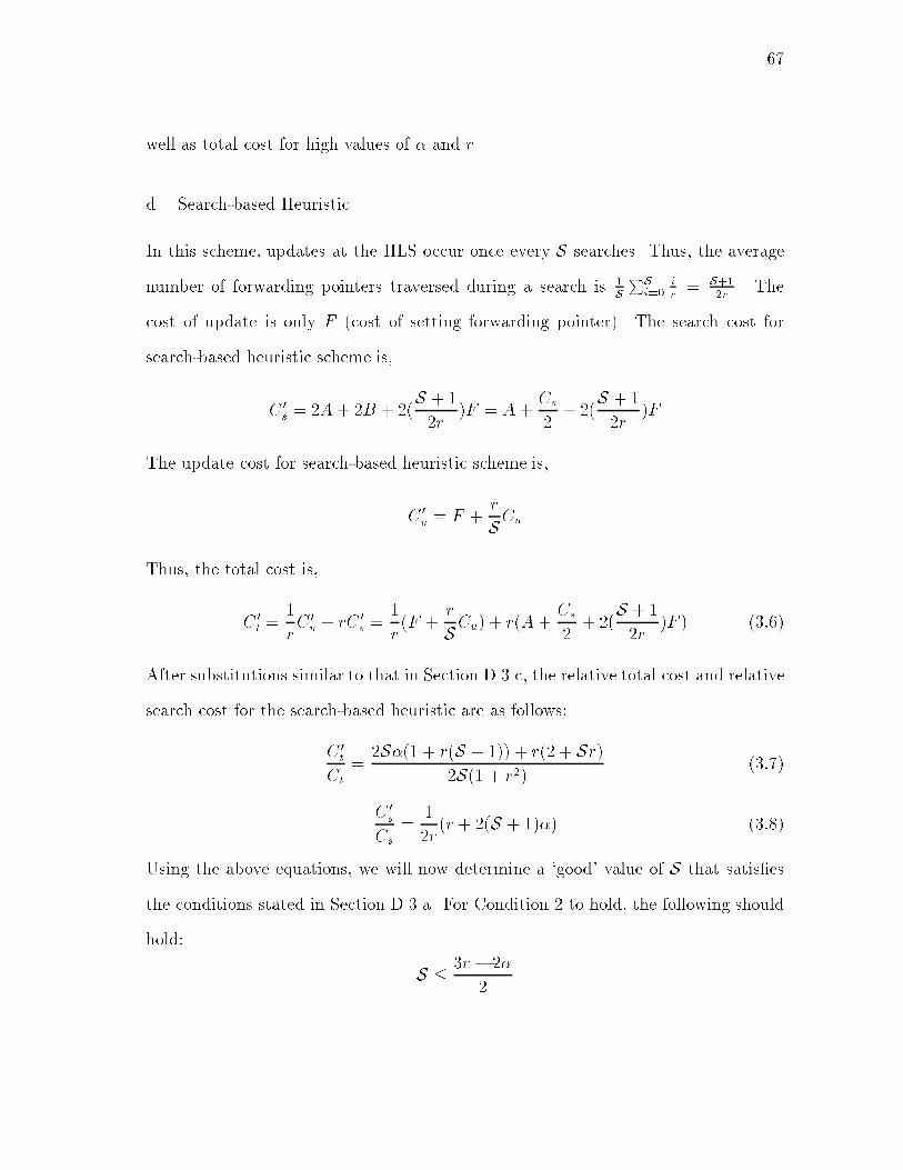
67well as total cost for high values of � and r.d. Search-based HeuristicIn this scheme, updates at the HLS occur once every S searches. Thus, the averagenumber of forwarding pointers traversed during a search is 1S PSi=0 ir = S+12r . Thecost of update is only F (cost of setting forwarding pointer). The search cost forsearch-based heuristic scheme is,C 0s = 2A+ 2B + 2(S + 12r )F = A+ Cs2 + 2(S + 12r )FThe update cost for search-based heuristic scheme is,C 0u = F + rSCuThus, the total cost is,C 0t = 1rC 0u + rC 0s = 1r (F + rSCu) + r(A+ Cs2 + 2(S + 12r )F ) (3:6)After substitutions similar to that in Section D.3.c, the relative total cost and relativesearch cost for the search-based heuristic are as follows:C 0tCt = 2S�(1 + r(S + 1)) + r(2 + Sr)2S(1 + r2) (3:7)C 0sCs = 12r (r + 2(S + 1)�) (3:8)Using the above equations, we will now determine a `good' value of S that satis�esthe conditions stated in Section D.3.a. For Condition 2 to hold, the following shouldhold: S � 3r � 2�2

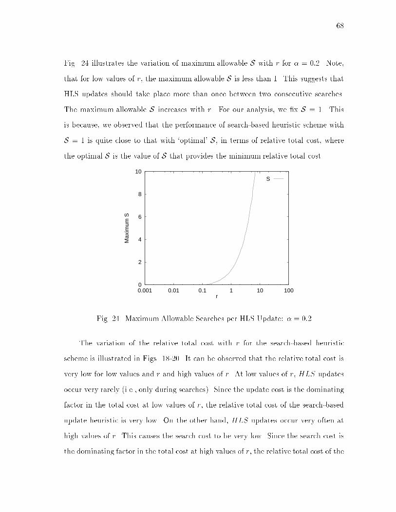
68Fig. 24 illustrates the variation of maximum allowable S with r for � = 0:2. Note,that for low values of r, the maximum allowable S is less than 1. This suggests thatHLS updates should take place more than once between two consecutive searches.The maximum allowable S increases with r. For our analysis, we �x S = 1. Thisis because, we observed that the performance of search-based heuristic scheme withS = 1 is quite close to that with `optimal' S, in terms of relative total cost, wherethe optimal S is the value of S that provides the minimum relative total cost.0

2

4

6

8

10

0.001 0.01 0.1 1 10 100

Max

imum

S

r

S

Fig. 24. Maximum Allowable Searches per HLS Update: � = 0:2The variation of the relative total cost with r for the search-based heuristicscheme is illustrated in Figs. 18-20. It can be observed that the relative total cost isvery low for low values and r and high values of r. At low values of r, HLS updatesoccur very rarely (i.e., only during searches). Since the update cost is the dominatingfactor in the total cost at low values of r, the relative total cost of the search-basedupdate heuristic is very low. On the other hand, HLS updates occur very often athigh values of r. This causes the search cost to be very low. Since the search cost isthe dominating factor in the total cost at high values of r, the relative total cost of the

69search-based heuristic is very low. However at moderate values of r, the performanceof search-based heuristic scheme is worse than the IS-41 scheme.Figs. 21-23 illustrate the variation of relative search costs with r for � =0:2; 0:5 and 0:8 respectively. It can be observed that the search cost is very highfor low values of r. This is because for small r, the HLS updates occur infrequently,and the moves frequently. Thus, each search has to traverse a long chain of forwardingpointers. Moreover, there is a rapid decrease in search costs as r increases. This isbecause the length of chain of forwarding pointers reduces as calls arrive more often.e. Observations� For movement-based heuristic to perform well over a wide range of r and �, asmall value of M should be chosen.� The relative total cost of the search-based heuristic is much lower than the IS-41 scheme and the movement-based heuristic scheme for low and high values ofr (r < 0:1 and r > 5). This is true for a wide range of �. However, the searchcost of the search-based heuristic is unacceptably high for low values of r.� For moderate values of r (0:1 < r < 5), the relative total cost of the movement-based heuristic scheme is lower than the IS-41 scheme and the search-basedheuristic scheme. However, this is true only for low values of � (� 0:5). Athigh values of �, a small value M (M < 3) should be chosen for movement-based heuristic scheme to perform well for moderate r. Also search cost ofmovement-based heuristic is unacceptably high for high values of �.Thus, it can be concluded that although forwarding pointers do reduce the totalnetwork load, the search cost (i.e., call set-up time) increases. In the next section wepresent a search-update strategy to reduce the search cost.

70E. A Search-Update StrategyThe search cost could be reduced by eliminating the cost of querying the HLS for thedestination host. This can be achieved by having a location entry at the src ls (inFig. 16) pointing to the start of the chain of forwarding pointers. This is called a\search-update". A search-update occurs after a successful search, when the locationserver of the requesting host updates the location information corresponding to themobile host. Search-updates might reduce the search cost (call set-up time). In thiswork, we will use a particular search-update strategy called jump update.1. Jump UpdateIn jump update a location entry is created at the location server (src ls) of thecaller (src) for the destination host (dest) after a successful search. As stated earlier,for search-based heuristic, an update at the HLS take place only after a search. Forjump update, in addition to updating the HLS, the location information of dest atsrc ls is also updated. If there were no location entries for dest at src ls, a locationentry is created. The cost of jump update is the cost of setting a forwarding pointer.The motivation behind this kind of update is based on the assumption that srccommunicates frequently with dest. Therefore, the subsequent search by src for destwill potentially be lower.2. Altered Search Procedure for Search-UpdatesThe search procedure needs to be altered to make use of the location information (ifavailable) at the location server. If dest is not in the registration area of src ls, checkif src ls has a location entry for dest. The location entry for dest at src ls might beeither the current location of dest, or the start of a chain of forwarding pointers to

71the current location of dest. Thus, when the location entry can be found in src ls, aHLS query could be avoided. The chain of forwarding pointers is traversed to get tothe current location of dest. Else, if the location entry for dest is not found in src ls,follow the previously explained search procedure (Section D.2.c).3. Forwarding Pointer Maintenance for Search-UpdatesIn the forwarding pointer maintenance procedure described in Section D.2.d, we werenot concerned about the stale forwarding pointers at the location servers, because allthe searches (Section D.2.c) went to the HLS �rst. We ensure that the HLS doesnot have stale location information by updating the HLS at least once every Tpurgeunits of time. The location servers also purge forwarding pointers that are older thanTpurge units of time, thus, ensuring that stale forwarding pointers are not encounteredduring a search. However, if the search procedure of a host is altered as in Section E.2it should be ensured that the forwarding pointers at the location server are not staleat any point of time.A location information at a location server is purged or updated (when search-update scheme is used) in the following events:� During search-updates.� When an HLS update takes place.� When a mobile host disconnects.Search-updates: The timestamp of a forwarding pointer for the host is updated withthe current time at the location server whenever a search-update for the host takesplace at the location server.

72HLS update: For the movement-based heuristic, HLS update takes place after Mregistration area crossings. Apart from the periodic purging (due to timeouts), wehave to purge the forwarding pointers which become stale after an update at theHLS. This will bound the maximum length of forwarding pointers traversed duringa search to (M� 1). Such purging is possible, if the pointers are bi-directional, i.e.,there are backward pointers in addition to the forwarding pointers. Therefore, afteran HLS update, purge messages are sent to the location servers containing staleforwarding pointers for the host. These location servers are determined using thebackward pointers. If forwarding pointers are purged after an HLS update, then theaverage number of pointers for a host in the network at any time is upper boundedby (M� 1) + rM. The explanation is as follows: The maximum length of the chainbefore an update at the HLS is (M�1), i.e, there is a maximum of (M�1) locationservers which have a forwarding pointer for a host due to moves before anHLS updatetakes place for the host. If search-updates are used, then each call for the host froma location server will lead to a forwarding pointer for the host at the location server.The average number of calls that can occur before an HLS update is rM. Therefore,the average number of location servers that have forwarding pointers created due tosearch-updates is upper bounded by rM. This is because there can be more thanone call from the area served by a location server. Therefore, for the movement-basedheuristic, the average number of purge messages sent during an HLS update is upperbounded by ((M� 1) + rM).If search-based heuristic is used, both HLS update and search-update take placeduring a search. The average number of moves made by the user between two searchesis 1r . Therefore, due to moves, the average number of location servers with forwardingpointers for the host is upper bounded by 1r . This is because the host may visit thesame cell. In addition, there is at most one location server that has a forwarding

73pointer for the host due to the previous search-update. Therefore, for the search-based heuristic, the average number of purge messages sent during an HLS updateis upper bounded by (1 + 1r ).Disconnection: Disconnections can also cause inconsistency in location information.If a host disconnects, its location information should be purged from all locationservers. The HLS of the host will know the last location of the host before it dis-connects (Appendix A). The HLS will also know the location of the host wheneverit reconnects/switches ON (Appendix A). However, if the host switches ON at alocation di�erent from the location where it had earlier disconnected, the locationservers which had forwarding pointers to the old location, have stale and incorrectinformation. Thus, if the altered search procedure (Section E.2) is used, we need topurge the stale and incorrect location information at these location servers. This willrequire purge messages to be sent to the location servers which have the forwardingpointers for the disconnected host. Subsequent search for the host initiated fromthese location servers will be forwarded to the HLS of the host. The HLS will nothave incorrect location information of the host. Any search query for a disconnectedhost initiated from these location servers while the purge is in progress will lead toa location server lsi which has no information of the host. The location server lsisends back an error message to the location server which initiated the search. Uponreceiving an error message, the location server will purge its forwarding pointer, andforward the search query to the HLS of the host.Forwarding pointer maintenance for search-updates require messages to be sentover the network. We include the purge costs in the update cost during our analysisof the search-update scheme. Since we are mainly concerned with the network loaddue to host movement, we do not consider the network load due to disconnections in

74our analysis. 4. Performance Analysis of Search-Update SchemeIn the analysis presented here, we assume that Tpurge is large enough (as compared tothe time period between two HLS updates due to heuristics) such that HLS updatesdue to timeout form a small fraction of all HLS updates. Therefore, we assume thatupdates at the HLS take place only upon searches (with search-based heuristic) orupon moves (with movement-based heuristic). Let:� s = Hit probability. It is the probability that a forwarding pointer to the desti-nation host exists at the location server of the caller's registration area.� C 00u ; C 00s ; C 00su; C 00t are the update, search, search-update and total cost using for-warding pointers and search-updates. C 00t = 1rC 00u + r(C 00s + C 00su).� k0 = For a caller host, this is the average number of forwarding pointers traversedbefore locating the destination host when search-updates are used.a. Movement-based Heuristic and Search-UpdatesThe update cost for schemes using search-updates will also include the purge costsincurred due to forwarding pointer maintenance.C 00u = C 0u + 1M(purge cost)Purge cost is the cost of sending purge messages to all the location servers containingstale forwarding pointers for the host. As stated earlier, the average number offorwarding pointers for a host in the network when search-updates are used is upperbounded by ((M� 1) + rM). If we assume that the cost of sending a purge message

75is equal to the cost of setting or traversing a forwarding pointer, then the averagepurge cost is upper bounded by ((M� 1) + rM)F . Therefore,C 00u = C 0u + FM((M� 1) + rM)C 00s = s(cost(src mss! src ls) + cost(traversing the forwarding pointers fromsrc ls to curr ls) + cost(curr ls! src ls) +cost(src ls! src mss)) + (1 � s)(C 0s)= s(A+ k0F + k0F +A) + (1� s)(2A+ 2B + 2k0F )= 2A+ 2k0F + 2(1 � s)B= C 0s � �s(Cs2 �A) + F ((M� 1)� 2k0)� where,C 0s is the search cost for the movement-based heuristic scheme without search-udpates.As stated earlier, the cost of search-update, C 00su, is the cost of sending a message tosrc ls to create a location entry. Therefore, C 00su is equal to F .C 00t = 1rC 00u + r(C 00s + C 00su)= 1r �C 0u + FM ((M� 1) + rM)�+r�C 0s � (s(Cs2 �A) + F ((M� 1)� 2k0)) + F�We substitute F = �Cu, A� Cu, Cs = Cu, C 0t = 1rC 0u + rC 0s. The expressions for C00tCtand C00sCs are as follows:C 00tCt = C 0tCt � r1 + r2 rs2 + r�((M� 1) � 2k0)� �((r + 1)M� 1)rM � r�)! (3:9)C 00sCs = C 0sCs � �s2 + �(M� 1 � 2k0)� (3:10)

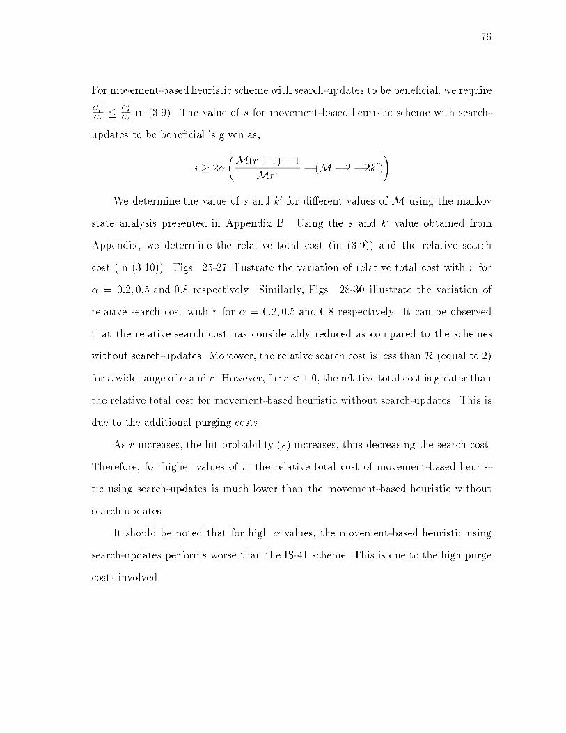
76For movement-based heuristic scheme with search-updates to be bene�cial, we requireC00tCt � C0tCt in (3.9). The value of s for movement-based heuristic scheme with search-updates to be bene�cial is given as,s � 2� M(r + 1)� 1Mr2 � (M� 2 � 2k0)!We determine the value of s and k0 for di�erent values of M using the markovstate analysis presented in Appendix B. Using the s and k0 value obtained fromAppendix, we determine the relative total cost (in (3.9)) and the relative searchcost (in (3.10)). Figs. 25-27 illustrate the variation of relative total cost with r for� = 0:2; 0:5 and 0:8 respectively. Similarly, Figs. 28-30 illustrate the variation ofrelative search cost with r for � = 0:2; 0:5 and 0:8 respectively. It can be observedthat the relative search cost has considerably reduced as compared to the schemeswithout search-updates. Moreover, the relative search cost is less than R (equal to 2)for a wide range of � and r. However, for r < 1:0, the relative total cost is greater thanthe relative total cost for movement-based heuristic without search-updates. This isdue to the additional purging costs.As r increases, the hit probability (s) increases, thus decreasing the search cost.Therefore, for higher values of r, the relative total cost of movement-based heuris-tic using search-updates is much lower than the movement-based heuristic withoutsearch-updates.It should be noted that for high � values, the movement-based heuristic usingsearch-updates performs worse than the IS-41 scheme. This is due to the high purgecosts involved.

770.4

0.5

0.6

0.7

0.8

0.9

1

1.1

1.2

0.01 0.1 1 10

Rel

ativ

e T

otal

Cos

t

Call Mobility Ratio (r)

M=2M=3M=4

Search-based

Fig. 25. Relative Total Costs (with Search Updates): � = 0:20.8

0.9

1

1.1

1.2

1.3

1.4

1.5

1.6

1.7

1.8

0.01 0.1 1 10

Rel

ativ

e T

otal

Cos

t

Call Mobility Ratio (r)

M=2M=3M=4

Search-based

Fig. 26. Relative Total Costs (with Search Updates): � = 0:5

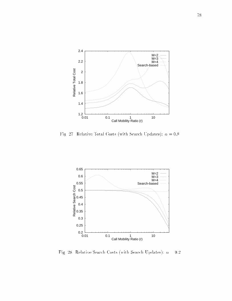
781.2

1.4

1.6

1.8

2

2.2

2.4

0.01 0.1 1 10

Rel

ativ

e T

otal

Cos

t

Call Mobility Ratio (r)

M=2M=3M=4

Search-based

Fig. 27. Relative Total Costs (with Search Updates): � = 0:80.2

0.25

0.3

0.35

0.4

0.45

0.5

0.55

0.6

0.65

0.01 0.1 1 10

Rel

ativ

e S

earc

h C

ost

Call Mobility Ratio (r)

M=2M=3M=4

Search-based

Fig. 28. Relative Search Costs (with Search Updates): � = 0:2

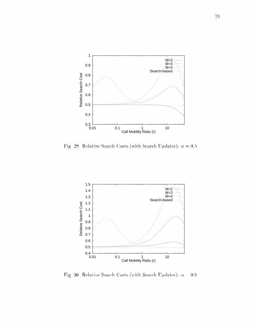
790.3

0.4

0.5

0.6

0.7

0.8

0.9

1

0.01 0.1 1 10

Rel

ativ

e S

earc

h C

ost

Call Mobility Ratio (r)

M=2M=3M=4

Search-based

Fig. 29. Relative Search Costs (with Search Updates): � = 0:50.4

0.5

0.6

0.7

0.8

0.9

1

1.1

1.2

1.3

1.4

1.5

0.01 0.1 1 10

Rel

ativ

e S

earc

h C

ost

Call Mobility Ratio (r)

M=2M=3M=4

Search-based

Fig. 30. Relative Search Costs (with Search Updates): � = 0:8

80b. Search-based Heuristic and Search-UpdatesAs stated earlier in Section D.2.d, we �x S = 1. Similar to the movement-basedheuristic, the update cost will also include the purge costs incurred due to forwardingpointer maintenance. As determined earlier in Section E.3, the upper bound onaverage purge cost for the search-based heuristic when search-updates are used is(1 + 1r )F . Therefore, C 00u = C 0u + r�1 + 1r�F where,C 0u is the update cost for search-based heuristic scheme without search-updates. Sim-ilar to the movement-based heuristic scheme with search-updates, the search cost forthe search-based heuristic with search-updates is,C 00s = C 0s � �s�Cs2 �A�+ 2F �1r � k0�� where,C 0s is the search cost for search-based heuristic scheme without search-updates. Thetotal cost C 00t is determined as,C 00t = C 00u + r(C 00s + C 00su)= C 0u + r(1 + 1r )F + r �C 0s � s(Cs2 �A) + 2F (1r � k0) + F�After substitutions, we determine C00tCt and C00sCs for the search-based heuristic schemewith search-updates as,C 00tCt = C 0tCt + r1 + r2 sr2 � �(r + 1)r + 2r�(1r � k0)� r�! (3:11)C 00sCs = C 0sCs � �s2 + 2�(1r � k0)� (3:12)For search-based heuristic scheme with search-updates to be bene�cial, we requireC00tCt � C0tCt in (3.11). The value of s for search-based heuristic scheme with search-

81updates to be bene�cial is given as:s � 2�(r + 1)r2 + 2��1 � 2r � 2k0�We determine the value of s and k0 using the markov state analysis presented inAppendix C. Using the s and k0 value obtained from Appendix, we determine therelative total cost (in (3.11)) and the relative search cost (in (3.12)). As seen in Figs.28-30, the relative search cost of the search-based heuristic scheme has considerablyreduced upon using search-updates. This has happened at the expense of a smallincrease in the relative total cost (Figs. 25-27). It should however be noted that athigh � values, search-updates are not suitable for search-based heuristic scheme. Thisis because of the high purging cost involved.c. Observations for Search-UpdatesIn this section we have presented a scheme for search-update. We augment the for-warding strategy with this search-update scheme and analyze its performance. Oneof our concerns with forwarding was the increase in search cost. It is somewhat al-leviated using search-updates; the search-based heuristic using search-updates hasvery low search costs for all values of r, and the movement-based heuristic usingsearch-updates have low search costs at high �. However, this saving in search costcomes with an increase in the total cost. This increase in total cost becomes verysigni�cant at high values of � (relative forwarding cost). It is observed that both theheuristics using search-updates performs poorly compared to IS-41 at high values of�. Therefore, search-updates are not suitable at high values of �.Fig. 31 presents a summary of the results. This �gure has been repeated fromSection A for convenience. As stated earlier, we divide the r space into three regions:low (r < 0:1), moderate (0:1 � r < 5) and high (r � 5). We divide the � space into

82two regions: low (� < 0:5), and high (alpha � 0:5).This �gure gives us a fair idea about when forwarding pointers and search-updates are bene�cial. If they are bene�cial, the table shows which combinationperforms the best.r

α

Low

High

Search-basedwith

Moderate

(M<5)

Movement-

Search-Updates

based

Movement-based(M<3)

Search-based

Low High

Movement-basedwith

Search-Updates

(M<5)Fig. 31. Performance ChartF. Fault ToleranceThe use of forwarding pointers introduces the issue of corruption/omission of a for-warding pointer due to a transient failure at a location server. It is assumed that theprotocol software is stored in some stable storage and hence does not get corrupteddue to these failures. Thus, if a location server crashes and recovers, the locationinformation (includes forwarding pointers) stored in the volatile memory may be ini-tialized randomly.Fault tolerance requires that regardless of the initial state, the system will even-tually converge to the correct state [18, 19]. The correct state in the scope of locationmanagement is that the location servers have the correct location information of thehosts. To recover from forwarding pointer corruption due to a transient failure, thelocation servers have to periodically send the pointer information to other locationservers reachable using the bi-directional pointers. An inconsistency can occur if a

83location server ls has a pointer for a host h to another location server ls1, and thelocation information of h at ls1 is corrupted by a transient failure. Thus, periodicexchange of information along the bi-directional pointers will ensure consistent for-warding pointer information to be stored in the location servers. Apart from theforwarding pointers, the host database (which stores the cell location of the host inits registration area) at the location server should also be fault tolerant. This willrequire periodic exchange of information between the MSSs in the registration areaand the location server. An inconsistency can occur if according to the location serverdatabase, a host is located in more than one cell, or not located in any cell althoughthe host is present in some MSS's cell in the registration area.If the location server crashes and recovers at a later time, its database will beinitialized to an inconsistent state with respect to the rest of the system. Thus, thesystem will have to eventually converge to the correct state. This can be ensured inthe following manner. The failed location server, upon recovery, informs the MSSsin its registration area and the other neighboring location servers about its recov-ery. Upon receiving the recovery message from the location server, the other locationservers check their forwarding pointer database for any forwarding pointers to/fromthe recovered location server. This is possible because we assume bi-directional point-ers. The location servers will send the forwarding pointer information to the recoveredlocation server, which in turn will update its forwarding pointer database. TheMSSsupon receiving the recovery message from the location server send the list of hostsin their cell to the location server so that the location server can initialize the hostdatabase (which stores the cell location of the host in its registration area).The table which represents the mapping of each mobile host to its home locationserver is assumed to be stored in the stable storage (e.g., disk) and thus is una�ectedby any failures. It is a safe assumption because this table needs to be always error-free

84and consistent with rest of the system (which includes other location servers), and isalso not updated as often as the forwarding pointer database or the host database.G. Memory OverheadA limitation of the forwarding pointer approach could be the memory overhead atthe location servers. In this section we try to analyze the memory overhead of theforwarding pointers. To assist in our analysis, we classify the pointers into two types:� Forwarding Pointers: A forwarding pointer for a host is created at a locationserver when the host goes out of the location server's registration area.� Bi-directional Pointers: This is required if the network needs to be fault-tolerant, or if search-updates are going to be used. In this case, a pointerfor a host is created at a location server when, (i) the host enters the locationserver's registration area, (ii) the host goes out of the location server's regis-tration area, or (iii) there is a call originating from the location server for thehost.We use the following notations and data for our analysis. The data is obtainedfrom [58]. Let:� U = Total number of users in the network = 2.87 million.� N = number of registration areas in the network = 128.� � = mean density of the users = 390/sq.km.� L = Registration area boundary length = 30.3 km.� v = average speed of the user = 5.6 km/hr.

85� � = Rate of call origination and delivery = 1.4/hr/user.� B1 = Size of a forwarding pointer in bytes.� B2 = Size of a bi-directional pointer in bytes.� tp = purge time interval for the pointers.A forwarding pointer has the following �elds: (i) identity of the mobile user, (ii)identity of the next registration area (destination of the forwarding pointer), (iii)timestamp indicating the time of creation of the pointer, and (iv) purge time interval,tp. We assume that we require (8+4) bytes to store the timestamp and tp respectively.In our analysis, we assume tp is same for all the pointers and is equal to 1 hour. Thesize of a forwarding pointer B1 is given by d log2(U)+log2(N)8 e+12. Replacing the valueswe get, B1 = 16 bytes.The rate of registration area crossing R is given as �vL� [75]. Replacing the values,we obtain R = 5:85=s. Let the maximum number of pointers that exist at a locationserver at any time be P . Let us consider forwarding pointers �rst. Since pointers arecreated only due to moves, P = R � tp. The memory required for forwarding pointersis M1 = P �B1 = 5:85 � 3600 � 16 � 337Kbytes.Let us consider bi-directional pointers now. The bi-directional pointer will havethe following �elds: (i) identity of the mobile user, (ii) identity of the next registrationarea (destination of the forwarding pointer), (iii) identity of the previous registrationarea (source of the forwarding pointer), (iv) timestamp indicating the time of creationof the pointer, and (v) purge time interval, tp. Thus, the size of a bi-directional pointerB2 is given by d log2(U)+2�log2(N)8 e + 12. Replacing the values we get, B2 = 17 bytes.Bi-directional pointers are created due to moves in and out of the registrationarea, and also due to calls. Thus, P = 2 �R � tp + �UN � tp. The memory required for

86bi-directional pointers is M2 = P �B2 = (2 � 5:85 � 3600 + 1:4 � 2:87 � 106=128) � 17 �1250Kbytes.The �gures above indicate the memory overhead required to implement the for-warding pointer scheme is insigni�cant when compared to the savings in terms ofnetwork bandwidth.H. Estimation of Call-Mobility Ratio rAs stated earlier, the performance of the proposed scheme depends on the call-mobility ratio (r) and the relative cost of forwarding pointers (�). High networkload is encountered if forwarding strategies are applied in networks where � is highand users have low r. The value of � is network dependent and should be known tothe system designer. However, user's call-mobility ratio is not known a priori to thesystem designer. Thus, it is important to estimate the call-mobility ratio of the usersso that the proper forwarding strategy could be applied. Various techniques havebeen proposed in literature to estimate r. A detailed investigation of the algorithmsfor estimating r, namely, running average, and reset-K were presented in [36]. InChapter IV [46], we propose algorithms to estimate r based on the history of calland mobility patterns. The basic assumption behind these algorithms are that pasthistory of the user's call mobility patterns will re ect the behavior in future.I. Comparison with Other Centralized SchemesOur work presented in this chapter [49, 50] di�ers from other centralized schemes [36,37] in the following respect:� A new heuristic (search-based) is proposed in this work. In [37] only movement-based heuristic is discussed.

87� This chapter studies the impact of combining forwarding and caching on theperfomance. We show that caching in addition to forwarding does improveperformance over schemes that employ only forwarding.� However, combining caching and forwarding brings about unique problems withforwarding pointer maintenance. In this chapter we propose schemes for for-warding pointer maintenance. We also account for the overhead incurred due tomaintenance in our analysis. Forwarding pointer maintenance and its associatedcost was not taken into account in [37].� We propose schemes to make location management strategy robust in the pres-ence of failures.� To assist in maintenance and fault-tolerance, we employ bi-directional pointersinstead of uni-directional pointers [37].J. SummaryThis chapter presents location management strategies using forwarding pointers andsearch-updates for network architectures with HLSs. Also presented are two heuris-tics to limit the length of the chain of forwarding pointers namely, movement-basedheuristic and search-based heuristic. We analyze the performance of these heuristics,and compare them with the scheme used in the IS-41 standard. It is observed thatusing forwarding pointers is bene�cial for most of the call-mobility ratios. However,the search cost of some of the schemes became very high and unacceptable for someparameter values. A scheme for search-update is presented to reduce the search costs.The performance of location strategies using forwarding pointers and search-updatesare analyzed.

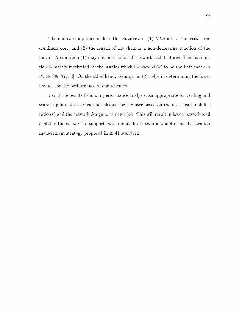
88The main assumptions made in this chapter are: (1) HLS interaction cost is thedominant cost, and (2) the length of the chain is a non-decreasing function of themoves. Assumption (1) may not be true for all network architectures. This assump-tion is mainly motivated by the studies which indicate HLS to be the bottleneck inPCNs [36, 37, 58]. On the other hand, assumption (2) helps in determining the lowerbounds for the performance of our schemes.Using the results from our performance analysis, an appropriate forwarding andsearch-update strategy can be selected for the user based on the user's call-mobilityratio (r) and the network design parameter (�). This will result in lower network loadenabling the network to support more mobile hosts than it would using the locationmanagement strategy proposed in IS-41 standard.

89CHAPTER IVDISTRIBUTED LOCATION MANAGEMENTA. IntroductionAs the cell size decreases, the number of calls transferred from one cell to anotherincreases. This causes the signalling tra�c to increase and spurs requirements formore e�cient location management schemes. We believe that the signalling tra�cgenerated by moving hosts in a distributed location management scheme will be lowerthan the current existing centralized algorithms (Chapter III). This improvementcan be accomplished by storing the location information of a mobile host in variouslocation servers. The network architecture consists of a hierarchy of location serverswhich are connected to themselves and to the base stations by a static network.Another advantage of hierarchical schemes is that the location address of a host canbe permanent. This is a desirable feature for a user who want the same address (e.g.,telephone number) associated with them for their entire life, irrespective of whetherthey change service providers or residence. However, in centralized schemes usinghome location servers (HLS), the user's address determines the HLS of the user. Ifa user changes service providers, there is a strong possibility that the HLS of theuser will also change. Same will be true if the user shifts to a new residence. Forexample, if a user is a resident of Texas, the user's HLS will typically be somewherein Texas. Now, if the user wishes to shift residence to New York, the user's HLS willno longer be in Texas for it will be cost prohibitive. Instead, the user will have a newHLS somewhere in New York. This will change the user's address. Thus, life-longaddressing will not be possible in HLS based schemes without decoupling the HLSfrom service providers and geographical locations.

90In this chapter we present several location management strategies based on ahierarchical tree structure database. These strategies try to satisfy the goal of pro-viding e�cient searches and updates. A location management strategy is a combi-nation of a search strategy, an update strategy, and a search-update strategy. Staticlocation management uses one �xed combination of search, update and search-updatestrategies. This chapter presents the results of simulations carried out to evaluate theperformance of various static location management strategies for various call-mobilitypatterns.If the system designer has a priori knowledge of the call-mobility pattern of theuser, the strategy which performs best for the given values of call and mobility can beselected. However, this information is not always available. Thus, there is a need foradaptive location management. The basic philosophy behind adaptive managementis that the past history of the system will re ect the behavior in the future, andhence by keeping track of the past history and modifying the management strategyaccordingly, one expects to perform well for any call-mobility pattern. In this chapterwe present preliminary ideas and results for adaptive location management.Unlike in previous chapter, we resort to simulations to analyze the schemes pre-sented in this chapter so that we can accomodate non-uniform call-mobility patterns.Real-life call-mobility traces are expected to be non-uniform and we show in thischapter that adaptive location management performs well in such conditions.The review of related work in location management can be found in Chapter III.This chapter is organized as follows. Section B presents the static location manage-ment strategies, and Section C presents the simulation results for the various staticlocation management strategies. Section D presents the adaptive location manage-ment scheme and summary is presented in Section E.

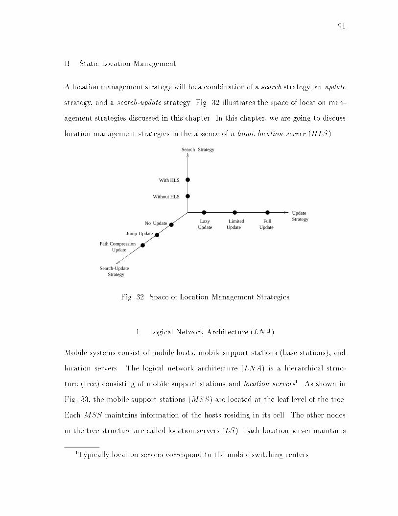
91B. Static Location ManagementA location management strategy will be a combination of a search strategy, an updatestrategy, and a search-update strategy. Fig. 32 illustrates the space of location man-agement strategies discussed in this chapter. In this chapter, we are going to discusslocation management strategies in the absence of a home location server (HLS).Search

With HLS

Without HLS

Lazy Limited Full

Strategy

Update

Update

UpdateJump

NoUpdate Update Update

Strategy

Path CompressionUpdate

Search-UpdateStrategyFig. 32. Space of Location Management Strategies1. Logical Network Architecture (LNA)Mobile systems consist of mobile hosts, mobile support stations (base stations), andlocation servers. The logical network architecture (LNA) is a hierarchical struc-ture (tree) consisting of mobile support stations and location servers1. As shown inFig. 33, the mobile support stations (MSS) are located at the leaf level of the tree.Each MSS maintains information of the hosts residing in its cell. The other nodesin the tree structure are called location servers (LS). Each location server maintains1Typically location servers correspond to the mobile switching centers.

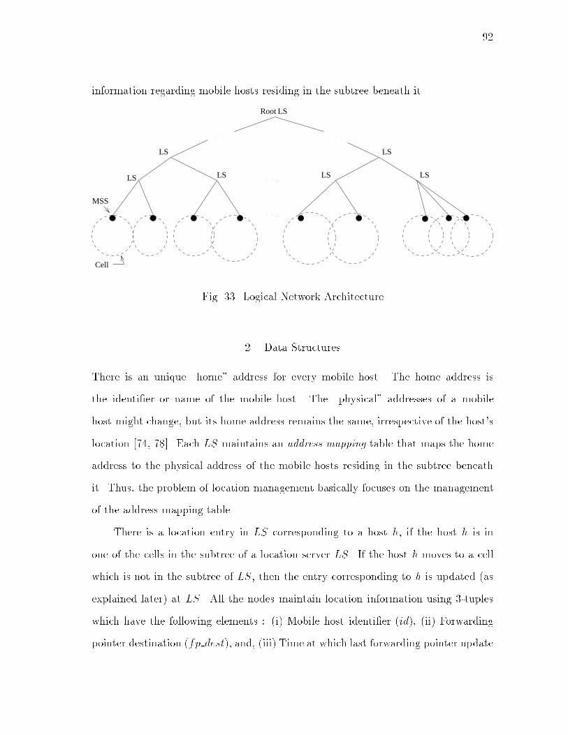
92information regarding mobile hosts residing in the subtree beneath it.LS

LS

LS LS

LS

LS

Cell

MSS

Root LS

Fig. 33. Logical Network Architecture2. Data StructuresThere is an unique \home" address for every mobile host. The home address isthe identi�er or name of the mobile host. The \physical" addresses of a mobilehost might change, but its home address remains the same, irrespective of the host'slocation [74, 78]. Each LS maintains an address mapping table that maps the homeaddress to the physical address of the mobile hosts residing in the subtree beneathit. Thus, the problem of location management basically focuses on the managementof the address mapping table.There is a location entry in LS corresponding to a host h, if the host h is inone of the cells in the subtree of a location server LS. If the host h moves to a cellwhich is not in the subtree of LS, then the entry corresponding to h is updated (asexplained later) at LS. All the nodes maintain location information using 3-tupleswhich have the following elements : (i) Mobile host identi�er (id), (ii) Forwardingpointer destination (fp dest), and, (iii) Time at which last forwarding pointer update

93took place (fp time). Each location server maintains a 3-tuple for each mobile hostresiding in the subtree beneath it, and each mobile support station maintains a 3-tuplefor each mobile host residing in its cell.At the location servers and theMSS, forwarding pointer destination (fp dest) isthe location of the mobile host. At theMSS, the fp time value for a host residing inits cell isNULL. Let us illustrate the use of forwarding pointers with an example. Letus suppose that we are using a strategy which uses forwarding pointers for locationupdates. Let a host h reside initially in cell c. The MSS of the cell c will have anentry (h;c; NULL). Let there be a location server L which maintains information ofthe hosts residing in cell c. There will be an entry (h; c; tl) corresponding to host hat L, where tl is the local time at L at which the entry was recorded at L. Let hosth move to a new cell c0. Let t be the local time at the MSS of cell c at which thechange of location of h is recorded at theMSS. Let t0 be the local time at L at whichthe change of location of h is recorded at L. Thus, the location information of h willbe (h; c0; t0) at L, and, (h; c0; t) at MSS of cell c.A Note: The above data structures contain fp time �eld to store time. Thefp time entry for a data structure on a node, say v, contains the local time at node vwhen the data structure was last modi�ed. It should be noted that the correctness ofthe algorithms does not require the clocks at various nodes to be tightly synchronized.3. Initial ConditionsIt is assumed that, initially, the location information of the mobile hosts is storedin the corresponding location servers, i.e., each location server (LS) should have thecorrect location information for all the hosts residing in the cells in its subtree. Thus,the root location server should have the correct location information of all the hosts inthe system. Let us illustrate this with an example. In Fig. 34, nodes 1-7 are location

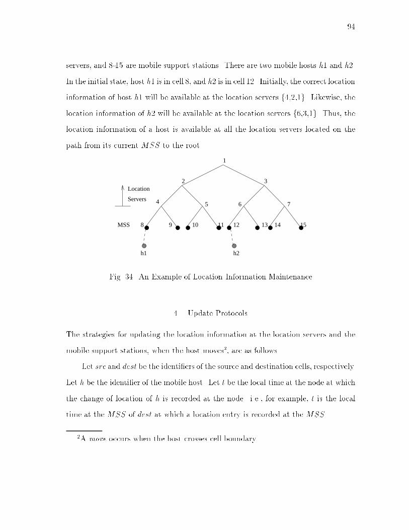
94servers, and 8-15 are mobile support stations. There are two mobile hosts h1 and h2.In the initial state, host h1 is in cell 8, and h2 is in cell 12. Initially, the correct locationinformation of host h1 will be available at the location servers f4,2,1g. Likewise, thelocation information of h2 will be available at the location servers f6,3,1g. Thus, thelocation information of a host is available at all the location servers located on thepath from its current MSS to the root.1

2 3

4 5 6 7

8 9 10 11 12 13 14 15

Location

Servers

MSS

h1 h2Fig. 34. An Example of Location Information Maintenance4. Update ProtocolsThe strategies for updating the location information at the location servers and themobile support stations, when the host moves2, are as follows.Let src and dest be the identi�ers of the source and destination cells, respectively.Let h be the identi�er of the mobile host. Let t be the local time at the node at whichthe change of location of h is recorded at the node. i.e., for example, t is the localtime at the MSS of dest at which a location entry is recorded at the MSS.2A move occurs when the host crosses cell boundary.

95a. Lazy Updates (LU)This is the simplest update scheme. Updates take place only at theMSS of the sourceand destination cells. A forwarding pointer is kept at the source MSS. The updatedentry at the source MSS becomes (h; dest; t). An entry for host h, (h; dest;NULL)is added at the destination MSS. The location information at the location serversare not updated. The cost of update is zero, because there are no update messagesbeing sent.b. Full Updates (FU)Upon a move, apart from the MSSs involved (i.e., the MSS of the source anddestination cells), location updates take place in all the LSs located on the path fromtheMSS of the source and destination cells to the root. The scheme and an examplefollows.Source cell:1. At the MSS : For host h, set fp dest = dest, and fp time = t. The updatedentry for host h at the MSS becomes (h; dest; t).2. All location servers on the path from src to the root : The MSS of src sendsupdate message to these location servers. Upon receipt of the update message,the location servers update the entry for h to (h; dest; tl), where tl is the localtime at the location server.Destination cell:1. At the MSS : An entry (h; dest;NULL) is added for host h. If there was anold entry for h, it is overwritten by this new entry. There can be only one entry

96per host in the MSS and the LS.2. All location servers on the path from dest to the root : TheMSS of dest sendsupdate message to these location servers. Upon receipt of the update message,the location servers create an entry (h; dest; tl), where tl is the local time at thelocation server. If there was an old entry, it is overwritten by this new entry.Therefore, in an H-level tree, the update cost per move is 2(H � 1), where, thecost metric is the number of messages. Let us illustrate this scheme with an example.Suppose in Fig. 34, host h1 moves from 8 to 14. Forwarding pointer to 14 will be keptat MSS 8. MSS 8 sends update message to f4,2,1g, and these location servers alsomaintain forwarding pointer to 14. An entry for h1 will be made at MSS 14. MSS14 sends update message to the location servers f7,3,1g, and these location serversalso make an entry for host h1.c. Limited Updates (LMU)Update in the location information takes place at a limited number of levels of locationservers in the tree. Here updates occur at m(< H) lower levels of location servers onthe path to the root. Updates at these location servers are similar to the FU scheme.The location servers at levels higher than m are not updated. Thus, the update costper move is 2m. Let us illustrate this scheme with an example. Let the value of m bechosen to be 1. Suppose in Fig. 34, host h1 moves from cell 8 to cell 14. Forwardingpointer to 14 will be kept at MSS 8. MSS 8 sends an update message to f4g, and 4maintains forwarding pointer to 14. An entry for h1 will be made at MSS 14. MSS14 sends an update message to f7g, and 7 makes an entry for host h1.

975. Search ProtocolIf a host h in cell C wants to communicate with another host h0, h has to know thelocation of h0. This requires that host h search for host h0. As stated earlier, we donot make explicit use of home location server (HLS) for searches. The search processin the absence of a HLS is as follows. If the mobile support station of C has nolocation information for h0, it forwards the location query to the next higher levellocation server on the path to the root. If that location server does not have anylocation information for h0, it again forwards the location query to the next higherlevel location server on the path to the root. This process repeats until a locationserver which has location information for h0 is reached. In this process if the rootlocation server is reached, and the root also does not have the location information forh0, then the root broadcasts to �nd out the location of the host h0. In our schemes wemake sure that the root has location information (as explained later), so the broadcastwill not be necessary. Once the location information (cell identi�er) for h0 is obtained,the location query is forwarded to the MSS of the cell. Host h0 is either in the cell ofMSS, or, MSS has a forwarding pointer corresponding to h0. If host h0 is in the cellof MSS, the search is complete. Else, a chain of forwarding pointers is traversed tillthe MSS containing the host h0 is reached. The search protocol is as shown in Fig.35. 6. Search-Update ProtocolsThe idea of manipulating forwarding pointers upon a successful search was earliersuggested in [21]. It was used to track objects in a decentralized object oriented com-puter system. Location management becomes more e�cient if the location updatesalso take place after a successful search. For example, suppose there is a host h that

98Initially, the search cell is C.Step 1 : If the MSS of the search cell has an entry for h0,If fp dest = search cell,host h0 is in the search cell. Search for h0 is complete.Else search cell = fp dest. Repeat step 1.Else forward the query to the next higher level location serveron the path to the root.Step 2 : If the location server has an entry (h0; fp dest; fp time) for h0search cell = fp dest. Go to step 1.Else If the location server is the rootRoot broadcasts to �nd out location of h0. The location server that hasan entry (h0; fp dest; fp time) forwards the location query to fp dest.Set search cell = fp dest. Go to step 1.Else Forward the query to the next higher level location serveron the path to the root.Go to Step 2. Fig. 35. Search Protocol

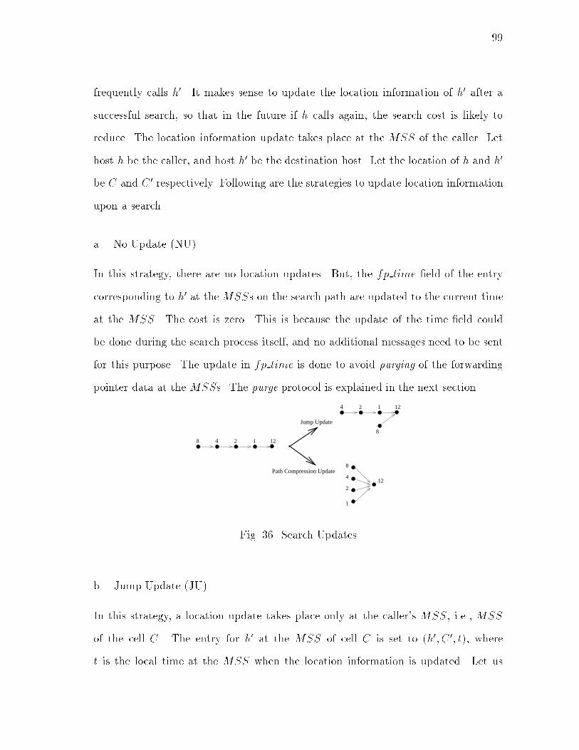
99frequently calls h0. It makes sense to update the location information of h0 after asuccessful search, so that in the future if h calls again, the search cost is likely toreduce. The location information update takes place at the MSS of the caller. Lethost h be the caller, and host h0 be the destination host. Let the location of h and h0be C and C 0 respectively. Following are the strategies to update location informationupon a search.a. No Update (NU)In this strategy, there are no location updates. But, the fp time �eld of the entrycorresponding to h0 at theMSSs on the search path are updated to the current timeat the MSS. The cost is zero. This is because the update of the time �eld couldbe done during the search process itself, and no additional messages need to be sentfor this purpose. The update in fp time is done to avoid purging of the forwardingpointer data at the MSSs. The purge protocol is explained in the next section.8

Jump Update

4 1212

8

4 1212

Path Compression Update

12

8

4

2

1Fig. 36. Search Updatesb. Jump Update (JU)In this strategy, a location update takes place only at the caller's MSS, i.e., MSSof the cell C. The entry for h0 at the MSS of cell C is set to (h0; C 0; t), wheret is the local time at the MSS when the location information is updated. Let us

100illustrate with an example. In Fig. 34, let host h1 call host h2. Suppose the locationinformation of h2 is available only at the location servers f6,3,1g. Using the searchprotocol described previously, the search path will be 8! 4! 2! 1! 12 (as shownin Fig. 36). During a jump update [21] following the search, the location informationat 8 is updated. Thus, 8 jumps from wherever it is in the forwarding path to havingthe current location information (as shown in Fig. 36). The update cost is 1. This isbecause only one message needs to be sent from theMSS of C 0 notifying the locationinformation of host h0.c. Path Compression Update (PCU)In this strategy, upon a successful search, a location update takes place at all thenodes in the search path. All the location servers on the search path have the entryof h0 updated to (h0; C 0; t), where t is the local time at the location server when thelocation information is updated. All the MSSs on the search path including thecaller's MSS have an entry of h0 updated to (h0; C 0; t), where t is the local timeat the MSS when the location information is updated. Let us illustrate with anexample. In Fig. 34, let host h1 call host h2. Suppose the location information of h2is available only at the location servers f6,3,1g. As shown in Fig. 36, the search pathwill be 8 ! 4 ! 2 ! 1 ! 12. During a path compression update [21] following thesearch, location updates take place at location servers f4,2,1g, and MSS 8. Thus, allthe nodes in the search path have the current location information (as shown in Fig.36). The update cost is the length of the search path, which in this example is 4.7. Purging of Forwarding PointersWe need to periodically purge the stale forwarding pointers at the location serversand the mobile support stations. This should be done in order to (i) save storage

101space at the nodes, and (ii) avoid storing stale location information. It does notmake any sense to keep the forwarding pointer information for a host h, if no otherhost is going to query this location server for the location information of h. We use adesign parameter purge interval (PI) to decide whether to purge a forwarding pointerinformation or not.The storage requirement at the location servers for forwarding pointers is a linearfunction of the purge time interval. For a typical personal communications network,it was determined that the memory required at the �rst level (the parents of the leaflevel nodes) location servers for PI equal to 1 hour, was about 340 Kbytes when nosearch updates were used, and, about 840 Kbytes when jump updates were used [46].Let the current time be curr time. If fp time 6= NULL, and curr time �fp time � PI, then the entry for the host is purged from theMSS 3. If curr time�fp time < PI, it means that there is some other host in the system which has recentlyused the forwarding pointer information of i.In the location servers, if curr time � fp time � PI for a host, the locationentry for the host is purged.a. Updating of Forwarding Pointers with a PurgeWhen LU and LMU strategies are used, the forwarding pointers at higher level loca-tion servers do not get updated, and become stale. Thus, these forwarding pointersget purged periodically. However, some of the searches for the host might reach thehigher levels. If the location servers at the higher levels do not have the informationof the host, the root has to broadcast to �nd out the location. To avoid this, the3Note that the fp time value for a host residing in the cell will be NULL. So weare considering hosts which are currently not residing in the MSS's cell and whoseforwarding pointer information is stored at the MSS.

102forwarding pointers at the location servers on the path to the root from the currentMSS must be updated periodically along with purging. This is achieved by the cur-rent MSS of each mobile host by sending a location update message to the locationservers on the path to the root.C. SimulationsA trade-o� exists between the cost of updates (upon moves and searches) and costof searches. The parameters that a�ect this trade-o� are (i) call frequency, and (ii)mobility. In this chapter we will evaluate the e�ects of mobility and call frequencyon the cost of updates, search-updates and searches. As stated earlier, the locationmanagement strategy is a combination of a search strategy, an update strategy and asearch-update strategy. The search protocol is the same for all location managementstrategies. A total of 9 static location strategies are obtained using above strategies forupdates and search-updates. We performed simulations to analyze the performance ofthe proposed location management strategies for various call frequency and mobilityvalues. The location management strategies simulated were obtained by choosingone update strategy (say XX, where XX = LU, FU or LMU) and one search-updatestrategy (say YY, where YY = NU, JU or PCU). The location management strategythus obtained is denoted as XX-YY. 1. ModelWe assume a binary tree as the logical network architecture for the simulations. Theheight of the tree is H. The number of location servers in the network is 2(H�1) � 1,and the number of mobile support stations (or the number of cells) is 2(H�1). Physicalproximity of the cells under the same location server is assumed. This will help in

103determining short and long moves. The height of the tree H was chosen to be 10 forthe simulations4. Thus, there were 512 cells in the network.The main aim of the chapter is to develop protocols for e�cient searches andupdates, i.e., reduce the number of messages due to location updates, without in-creasing the number of messages required for searches. We assume that the messagedelays are negligible. Since, message delays are small compared to the time betweencalls or moves, performance of the schemes will not be signi�cantly a�ected by thisassumption.Simulations were performed for two types of environments : (i) arbitrary movesand arbitrary callers, (ii) short moves and a set of callers. In type (i), the user canmove to any location (cell), and, get calls from any other host in the network. Thisis not necessarily true in real life, but it gives a fair idea of the performance of thelocation management schemes in such extreme conditions. Type (ii) is closer to reallife mobile environments. Users are expected to make a lot of short moves to nearbydestinations, and are expected to receive calls from a speci�c set of callers (e.g. family,business colleagues)5.a. Call and Mobility Distribution for Type (i)The time between moves of a host is assumed to follow an exponential distributionwith a mean M . The destination cell is chosen randomly among the 512 cells. Thetime between calls for a host is assumed to follow an exponential distribution with a4In existing networks like GSM or Internet, the height will be 3 to 4. Since a binarytree was assumed for the simulations, we needed to have higher number of levels tohave a sizeable number of cells in the network. However, similar performance trendsare expected for other networks.5The callers are assumed to be immobile. They are either part of the staticnetwork, or, do not leave their cell.

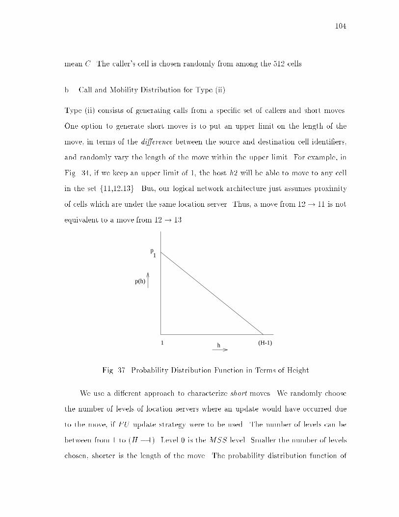
104mean C. The caller's cell is chosen randomly from among the 512 cells.b. Call and Mobility Distribution for Type (ii)Type (ii) consists of generating calls from a speci�c set of callers and short moves.One option to generate short moves is to put an upper limit on the length of themove, in terms of the di�erence between the source and destination cell identi�ers,and randomly vary the length of the move within the upper limit. For example, inFig. 34, if we keep an upper limit of 1, the host h2 will be able to move to any cellin the set f11,12,13g. But, our logical network architecture just assumes proximityof cells which are under the same location server. Thus, a move from 12! 11 is notequivalent to a move from 12! 13.p(h)

h1 (H-1)

p1

Fig. 37. Probability Distribution Function in Terms of HeightWe use a di�erent approach to characterize short moves. We randomly choosethe number of levels of location servers where an update would have occurred dueto the move, if FU update strategy were to be used. The number of levels can bebetween from 1 to (H � 1). Level 0 is the MSS level. Smaller the number of levelschosen, shorter is the length of the move. The probability distribution function of

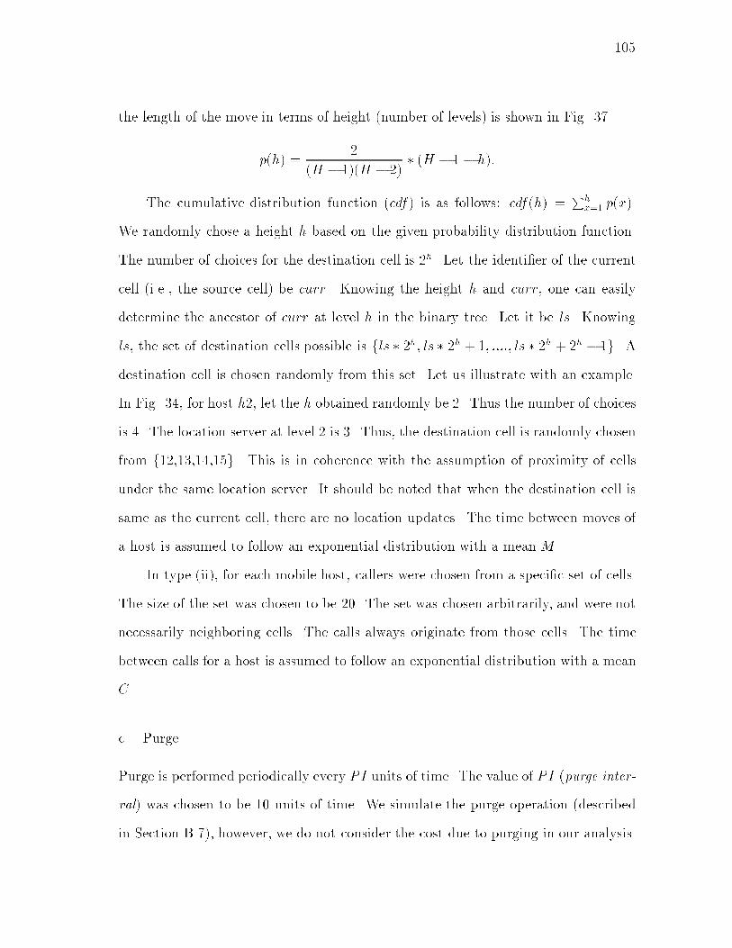
105the length of the move in terms of height (number of levels) is shown in Fig. 37.p(h) = 2(H � 1)(H � 2) � (H � 1� h):The cumulative distribution function (cdf) is as follows: cdf(h) = Phx=1 p(x).We randomly chose a height h based on the given probability distribution function.The number of choices for the destination cell is 2h. Let the identi�er of the currentcell (i.e., the source cell) be curr. Knowing the height h and curr, one can easilydetermine the ancestor of curr at level h in the binary tree. Let it be ls. Knowingls, the set of destination cells possible is fls � 2h; ls � 2h + 1; ::::; ls � 2h + 2h � 1g. Adestination cell is chosen randomly from this set. Let us illustrate with an example.In Fig. 34, for host h2, let the h obtained randomly be 2. Thus the number of choicesis 4. The location server at level 2 is 3. Thus, the destination cell is randomly chosenfrom f12,13,14,15g. This is in coherence with the assumption of proximity of cellsunder the same location server. It should be noted that when the destination cell issame as the current cell, there are no location updates. The time between moves ofa host is assumed to follow an exponential distribution with a mean M .In type (ii), for each mobile host, callers were chosen from a speci�c set of cells.The size of the set was chosen to be 20. The set was chosen arbitrarily, and were notnecessarily neighboring cells. The calls always originate from those cells. The timebetween calls for a host is assumed to follow an exponential distribution with a meanC.c. PurgePurge is performed periodically every PI units of time. The value of PI (purge inter-val) was chosen to be 10 units of time. We simulate the purge operation (describedin Section B.7), however, we do not consider the cost due to purging in our analysis.

1062. Cost ModelThe cost metric is the number of messages required for each operation (search, up-date, and search-update). Thus, the cost of an update is the number of locationservers which update the location information of the host. The cost of a search isthe number of location servers and mobile support stations visited before locatingthe host. Cost of a search-update is the number of location servers which update thelocation information of the host.The performance parameter of interest is the total cost, de�ned as the sum ofaverage update cost, average search cost, and the average search-update cost. Othercost metrics are also possible (For example, see Chapter III.D.3.a).3. ResultsSimulations were performed to analyze the performance of the various location man-agement strategies. Results were obtained for the two type of environments, Type (i)and (ii). The values of C and M were both varied from 1 to 15 units of time. Valueof C was changed to vary the time interval between two successive calls. Value ofM was changed to vary the mobility of the host. For example, C = 1 and M = 1characterizes a communication intensive and ultra-mobile environment.Type(i) : It was observed that the LU -PC strategy outperforms all the other strate-gies for all values ofM and C. Therefore, we have only plotted the curves for LU -PC.The strategies using FU and LMU su�ered due to the high cost of updates upon eachmove. LU -NU strategy su�ered due to very high search costs. Because the callerswere arbitrary, LU -JU strategy did not perform well as the update upon a successfulsearch was not helping in reducing the search cost. Fig. 38 plots the total cost for theLU -PC strategy as a function of C for di�erent values of M . As seen in the �gure,

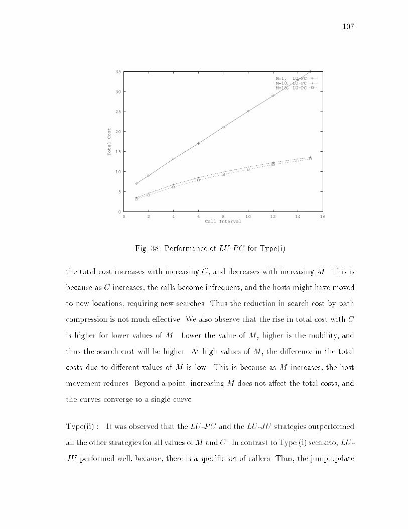
1070

5

10

15

20

25

30

35

0 2 4 6 8 10 12 14 16

Total Cost

Call Interval

M=1, LU-PCM=10, LU-PCM=15, LU-PC

Fig. 38. Performance of LU -PC for Type(i)the total cost increases with increasing C, and decreases with increasing M . This isbecause as C increases, the calls become infrequent, and the hosts might have movedto new locations, requiring new searches. Thus the reduction in search cost by pathcompression is not much e�ective. We also observe that the rise in total cost with Cis higher for lower values of M . Lower the value of M , higher is the mobility, andthus the search cost will be higher. At high values of M , the di�erence in the totalcosts due to di�erent values of M is low. This is because as M increases, the hostmovement reduces. Beyond a point, increasing M does not a�ect the total costs, andthe curves converge to a single curve.Type(ii) : It was observed that the LU -PC and the LU -JU strategies outperformedall the other strategies for all values ofM and C. In contrast to Type (i) scenario, LU -JU performed well, because, there is a speci�c set of callers. Thus, the jump update

1080

2

4

6

8

10

12

14

16

18

0 2 4 6 8 10 12 14 16

Total Cost

Call Interval

M=1, LU-PCM=10, LU-PCM=15, LU-PCM=1, LU-JUM=10, LU-JUM=15, LU-JU

Fig. 39. Comparison of LU -PC and LU -JU for Type(ii)at the caller is much more e�ective in reducing the search cost, because the caller isgoing to call the host again with a higher probability than in Type (i) environment.Fig. 39 plots the total cost for the LU -JU strategy and the LU -PC strategy as afunction of C for di�erent values ofM . As seen, LU -JU performs better than LU -PCin high-communication and low-mobility, and, low-communication and high-mobilityenvironments. In these environments, the search cost for LU -PC and LU -JU arecomparable. Since the search-update cost is same as the search cost for LU -PC, thetotal cost for LU -PC is simply twice the search cost. Whereas, the average search-update cost for LU -JU is equal to 1. Thus, the total cost of LU -JU is lower thanLU -PC. LU -PC performs better for other values ofM and C because the search costfor LU -JU becomes large compared to LU -PC. Fig. 40 demonstrates the averagesearch cost for the LU -JU strategy and the LU -PC strategy as a function of C fordi�erent values of M . As seen, LU -PC has a much lower search cost than LU -JU .

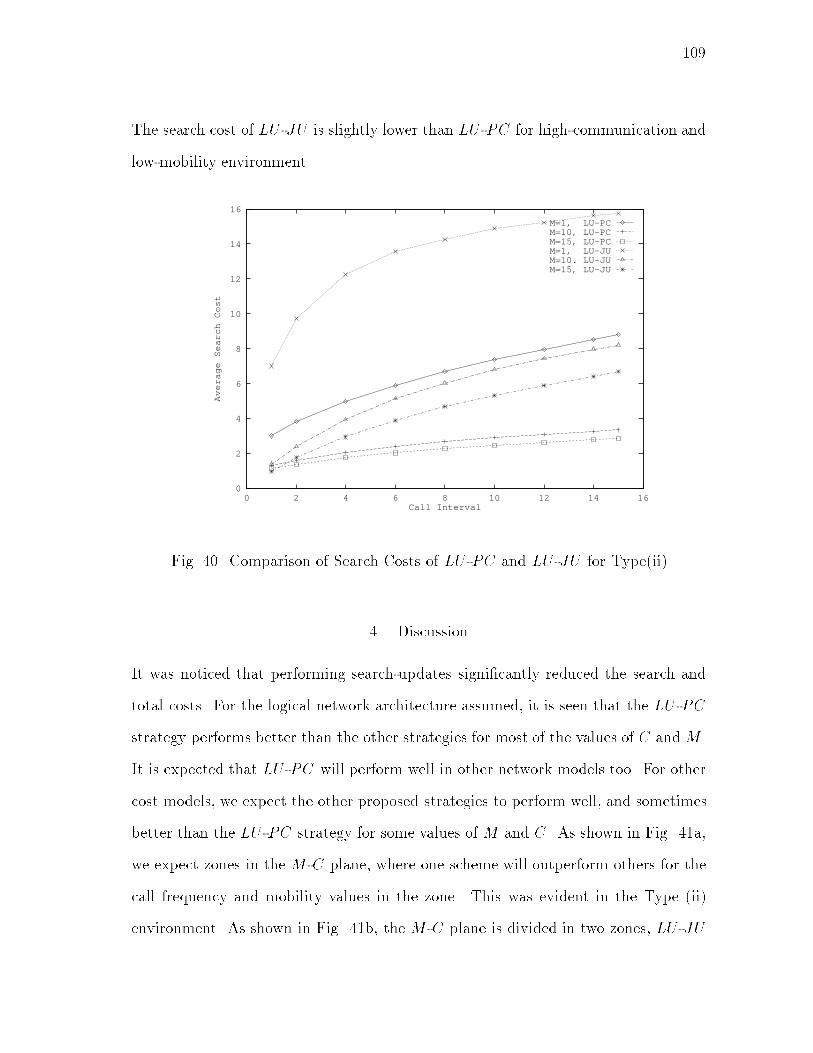
109The search cost of LU -JU is slightly lower than LU -PC for high-communication andlow-mobility environment.0

2

4

6

8

10

12

14

16

0 2 4 6 8 10 12 14 16

Average Search Cost

Call Interval

M=1, LU-PCM=10, LU-PCM=15, LU-PCM=1, LU-JUM=10. LU-JUM=15, LU-JU

Fig. 40. Comparison of Search Costs of LU -PC and LU -JU for Type(ii)4. DiscussionIt was noticed that performing search-updates signi�cantly reduced the search andtotal costs. For the logical network architecture assumed, it is seen that the LU -PCstrategy performs better than the other strategies for most of the values of C and M .It is expected that LU -PC will perform well in other network models too. For othercost models, we expect the other proposed strategies to perform well, and sometimesbetter than the LU -PC strategy for some values of M and C. As shown in Fig. 41a,we expect zones in the M -C plane, where one scheme will outperform others for thecall frequency and mobility values in the zone. This was evident in the Type (ii)environment. As shown in Fig. 41b, the M -C plane is divided in two zones, LU -JU

110and LU -PC. Thus, if the behavior of the mobile hosts (call frequency, mobility) isknown a priori, the designer can obtain such an M -C chart and decide which locationstrategy will best suit the system.C

M M

C

1

2

3

4

(a)

LU-JU

LU-PC

LU-JU

Generic Scenario Type (ii) Environment(b)Fig. 41. Partitioning of the M -C PlaneIn the next section we will present some preliminary ideas and results for adaptivelocation management.D. Adaptive Location ManagementThe system designer does not always have prior knowledge of the call-mobility patternof the hosts. In these cases, one would require a location management scheme thatcan dynamically change the update and search-update strategy, such that the overalloverhead incurred due to updates and searches is minimized. At the same time, wewould not want to use up the battery power of the mobile hosts to determine theappropriate strategy dynamically. We require theMSS to take up the responsibility.1. Data StructuresLet � be the current time at the mobile host h. M(h) is the sequence of moves ofthe host h. M(h) = fm1;m2; :::;mng, where, m1 = (t1; src; dest), i.e., element m1 is

111a move by the host h at time t1 from src to dest, and t1 < t2::: < tn. (The time ofmove is observed at the mobile host h.) Each element of the set M(h), mi, containstwo identi�ers { the source cell identi�er, and the destination cell identi�er. If bothidenti�ers are the same, then the host has not left the cell. This kind of entry is notnecessary (hence will not be present), because it does not a�ect the location database.But if the identi�ers are di�erent, the source cell should determine whether the moveis long or short.Cu(h) is the sequence of costs incurred due to updates upon the moves M(h).Cu(h) = fcu1; cu2; :::; cung, where cuj = cost of update upon a move mj.If another host h0 wants to communicate with h, and if h is not in the samecell or if the MSS of h0 does not know the cell identi�er of h, h0 has to search forh. A set S(h) is maintained at the current MSS of h. S(h) = fs1; s2; :::; sng, wheresi = (tsi; h0); i.e., there was a call from h0 for h at time tsi, and ts1 < ts2::: < tsn.Again, the time of call is observed at the mobile host h.Cs(h) is the sequence of costs incurred due to the searches S(h). Cs(h) =fcs1; cs2; :::; csng, where csj = cost of search sj. Csu(h) is the sequence of costs incurreddue to search-updates upon searches S(h). Csu(h) = fcsu1 ; csu2 ; :::; csung, where csuj= cost of search-update upon the search sj.The data structures are obtained as explained in the next section.2. Basic IdeaThe above data structures are stored at the current MSS of the host. They gettransferred to the new MSS during hando�. The decision of the type of updatesand search-updates are done by the current MSS. The current MSS uses the datastructures to determine the best suited strategy. The appropriate update and search-update strategy will be one of the proposed static location management update and

112search-update strategies.It is assumed that the mobile host h knows the identi�er of the cell it is currentlyresiding in. When a host h moves, h sends a message (containing the identi�er of itsold cell, and the time of move) to the new MSS. The new MSS forwards a copyof this message to the old MSS. The move is recorded as a new element mj in thesequence M(h). The old MSS takes a local decision (explained later) regarding theupdates. The cost of the update is recorded as a new element cuj in the sequence Cu.The new MSS requests the old MSS for the data structures corresponding to h. Ifthe new MSS makes any updates, the cost of the update is added to cuj in Cu.When a host h0 wants to communicate with h, and if h is not in the same cellor if the MSS of h0 does not know the identi�er of the cell of h, h0 has to search forh. A location query message is sent during the search. This message has a �eld tostore the search cost. At any time, the search cost �eld indicates the cost incurreddue to the search till now. The search cost gets incremented as the location querymessage is forwarded to a new location server or a mobile support station. Once h islocated, a new element sj is added to the sequence S(h) at the MSS of h. The timeof the call is the time observed at the mobile host h. The search cost is recorded asa new element csj to Cs(h). The MSS decides upon the appropriate search-updatestrategy. It is determined based on the call history (explained later). For example, ifa host h0 frequently calls host h, it makes sense to use JU to reduce the subsequentsearch cost for h0. The cost of the search-update is recorded as a new element csuj toCsu(h) at the MSS.

1133. Mobility and Call Frequencya. Determining MobilityLet at time t = � , M(h) = fm1;m2; :::;mng, where mn = (tn; src; dest), and tn � � .Thus, mn describes the move of host h that took place at time tn from a cell src toa cell dest. Thus, the average time interval between successive moves 4tavg = tn�t1n .We assume a system parameter maximum threshold move interval (MTMI). Ifthere are no moves by the host for MTMI amount of time, the host can be declaredto be immobile or stationary. The sets M(h) and Cu(h) maintained at the currentMSS are stale because the history does not re ect the behavior in future anymore.Therefore, they are deleted. In the absence of M(h) set, the host is assumed to havea high mobility upon the �rst move.We have de�ned two degrees of mobility { (i) low mobility, and (ii) high mobility.At any time � , let tn be the time of the last move by the host. If 4tavg < MTMI,the host has a high mobility, else if 4tavg �MTMI, the host has a low mobility.b. Determining Call FrequencyLet at time t = � , S(h) = fs1; s2; :::; sng, where sn = (tsn; h0), and tsn � � . sndescribes the call for host h from h0 that took place at time tsn. We de�ne an averagetime interval between calls for each caller to host h. The average time intervalbetween successive calls of caller h0, 4tsavg[h0] = Pn0i=14tsin0 , where, n0 is the number ofcalls made by h0, and the 4tsi's are the time intervals between two consecutive callsmade by host h0.We assume a system parameter maximum threshold call interval (MTCI). Ifthere are no calls by host h0 for MTCI amount of time, the host h0 can be declaredto have no communication with h. The elements corresponding to host h0 in the set

114S(h) are stale because the history does not re ect the behavior in future anymore.Therefore, they are deleted. In the absence of S(h) set, the caller h0 is assumed to bea frequent caller upon the �rst call of h0 to host h, i.e., 4ts1 = 0.Similar to mobility, based on the degree of call frequency, we have two types ofcaller { (i) non-frequent caller, and (ii) frequent caller. Then, if 4tsavg[h0] < MTCI,the caller is a frequent caller, else if 4tavg[h0] � MTCI, the caller is a non-frequentcaller.c. Size of Data StructuresThe maximum size n of the move set M(h) and search set S(h) can be chosen asa design parameter. Larger the value of n, better will be the learning of the hostbehavior, and thus a better predictability will be attained. However, the storagecapacity available at the MSS restricts the value of n. The MSS has to maintainthese sets for each mobile host in its cell. Thus, larger the value of n, larger is thestorage cost. 4. An ExampleIn this section we will present an example algorithm for adaptive location manage-ment. It is for the network model assumed for static location management strategies.The knowledge of Fig. 41b, and the fact that LU -PC is the best scheme for longmoves, will prove to be useful in dynamically determining the best strategy. Fromthe previous section, we have the techniques to classify the moves, calls and the mo-bility of the host. If a host has a lot of frequent callers, the host is being frequentlysearched, else, if a host has a lot of non-frequent callers, the host is not frequentlysearched. The algorithm is as shown in Fig. 42.We present an example where a simple algorithm adaptive as shown in Fig. 42

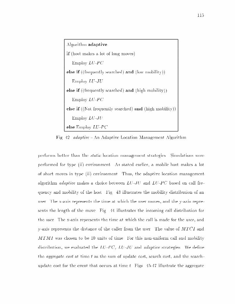
115Algorithm adaptiveif (host makes a lot of long moves)Employ LU -PC.else if ((frequently searched) and (low mobility))Employ LU -JU .else if ((frequently searched) and (high mobility))Employ LU -PC.else if ((Not frequently searched) and (high mobility))Employ LU -JU .else Employ LU -PC.Fig. 42. adaptive - An Adaptive Location Management Algorithmperforms better than the static location management strategies. Simulations wereperformed for type (ii) environment. As stated earlier, a mobile host makes a lotof short moves in type (ii) environment. Thus, the adaptive location managementalgorithm adaptive makes a choice between LU -JU and LU -PC based on call fre-quency and mobility of the host. Fig. 43 illustrates the mobility distribution of anuser. The x-axis represents the time at which the user moves, and the y-axis repre-sents the length of the move. Fig. 44 illustrates the incoming call distribution forthe user. The x-axis represents the time at which the call is made for the user, andy-axis represents the distance of the caller from the user. The value of MTCI andMTMI was chosen to be 10 units of time. For this non-uniform call and mobilitydistribution, we evaluated the LU -PC, LU -JU and adaptive strategies. We de�nethe aggregate cost at time t as the sum of update cost, search cost, and the search-update cost for the event that occurs at time t. Figs. 45-47 illustrate the aggregate

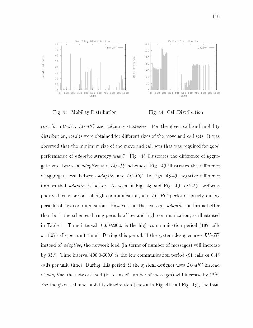
1160

10

20

30

40

50

60

70

80

0 100 200 300 400 500 600 700 800 900 1000

Length of move

Time

Mobility Distribution

’moves’

Fig. 43. Mobility Distribution 0

20

40

60

80

100

120

140

0 100 200 300 400 500 600 700 800 900 1000

Call Distance

Time

Caller Distribution

’calls’

Fig. 44. Call Distributioncost for LU -JU , LU -PC and adaptive strategies. For the given call and mobilitydistribution, results were obtained for di�erent sizes of the move and call sets. It wasobserved that the minimum size of the move and call sets that was required for goodperformance of adaptive strategy was 7. Fig. 48 illustrates the di�erence of aggre-gate cost between adaptive and LU -JU schemes. Fig. 49 illustrates the di�erenceof aggregate cost between adaptive and LU -PC. In Figs. 48-49, negative di�erenceimplies that adaptive is better. As seen in Fig. 48 and Fig. 49, LU -JU performspoorly during periods of high-communication, and LU -PC performs poorly duringperiods of low-communication. However, on the average, adaptive performs betterthan both the schemes during periods of low and high communication, as illustratedin Table 1. Time interval 100:0-200:0 is the high communication period (107 callsor 1:07 calls per unit time). During this period, if the system designer uses LU -JUinstead of adaptive, the network load (in terms of number of messages) will increaseby 33%. Time interval 400:0-600:0 is the low communication period (91 calls or 0:45calls per unit time). During this period, if the system designer uses LU -PC insteadof adaptive, the network load (in terms of number of messages) will increase by 12%.For the given call and mobility distribution (shown in Fig. 44 and Fig. 43), the total

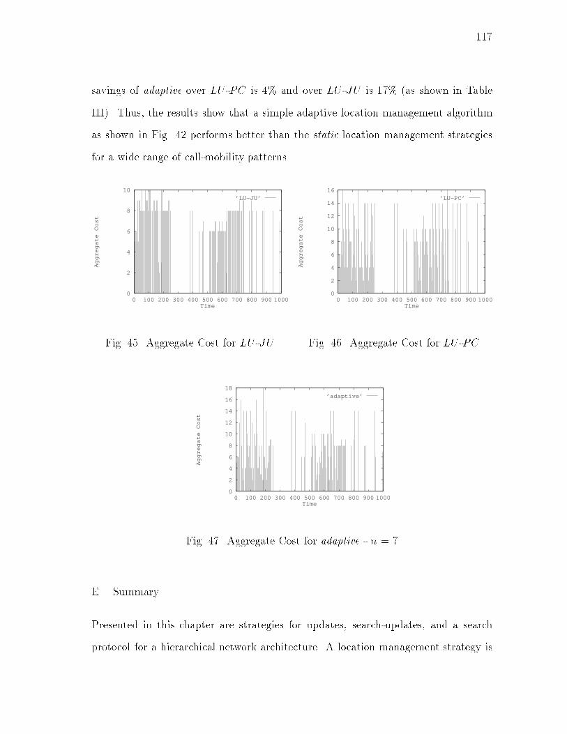
117savings of adaptive over LU -PC is 4% and over LU -JU is 17% (as shown in TableIII). Thus, the results show that a simple adaptive location management algorithmas shown in Fig. 42 performs better than the static location management strategiesfor a wide range of call-mobility patterns.0

2

4

6

8

10

0 100 200 300 400 500 600 700 800 900 1000

Aggregate Cost

Time

’LU-JU’

Fig. 45. Aggregate Cost for LU -JU 0

2

4

6

8

10

12

14

16

0 100 200 300 400 500 600 700 800 900 1000Aggregate Cost

Time

’LU-PC’

Fig. 46. Aggregate Cost for LU -PC0

2

4

6

8

10

12

14

16

18

0 100 200 300 400 500 600 700 800 900 1000

Aggregate Cost

Time

’adaptive’

Fig. 47. Aggregate Cost for adaptive - n = 7E. SummaryPresented in this chapter are strategies for updates, search-updates, and a searchprotocol for a hierarchical network architecture. A location management strategy is

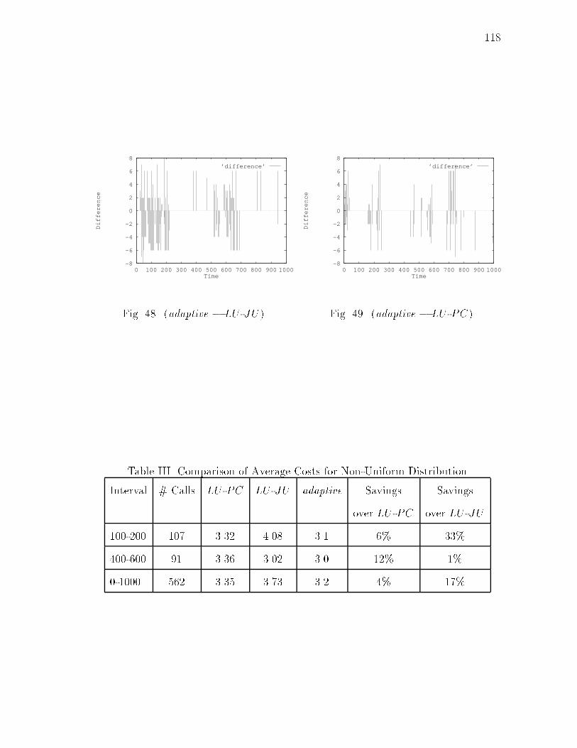
118-8

-6

-4

-2

0

2

4

6

8

0 100 200 300 400 500 600 700 800 900 1000

Difference

Time

’difference’

Fig. 48. (adaptive � LU -JU) -8

-6

-4

-2

0

2

4

6

8

0 100 200 300 400 500 600 700 800 900 1000

Difference

Time

’difference’

Fig. 49. (adaptive � LU -PC)Table III. Comparison of Average Costs for Non-Uniform DistributionInterval # Calls LU -PC LU -JU adaptive Savings Savingsover LU -PC over LU -JU100-200 107 3.32 4.08 3.1 6% 33%400-600 91 3.36 3.02 3.0 12% 1%0-1000 562 3.35 3.73 3.2 4% 17%

119a combination of the search strategy, a update strategy, and a search-update strat-egy. Simulations were carried out to evaluate the performance of the various locationmanagement strategies. It was noticed that performing search-updates signi�cantlyreduced total costs. For the logical network architecture assumed, it is seen thatthe LU -PC (combination lazy updates and path compression search-update) strat-egy performs better than the other strategies for most call-mobility patterns. It isexpected that LU -PC will perform well in other network models too.Static location management uses one combination of search, update and search-update strategies throughout the execution. In order to obtain good performanceusing static location management, the system designer should a priori have a fairidea of the call-mobility pattern of the users. The host behavior (call frequency,mobility) is not always available to the system designer. Thus, there is a need foran adaptive location management. In this chapter we present preliminary ideas foradaptive location management. The basic philosophy behind adaptive managementis that the past history of the system will re ect the behavior in the future andhence by keeping track of the past history and modifying the management strategyaccordingly, one expects to perform well for any call-mobility pattern. Simulationresults show that the performance of adaptive location management can be betterthan static location management. Adaptive location management results in lowernetwork load, enabling the network to support more mobile hosts than it would usingstatic location management.

120CHAPTER VROUTING IN DYNAMIC NETWORKSA. IntroductionA dynamic network composes of a set of mobile hosts that can communicate witheach other over the wireless links (direct or indirect) without any static networkinteraction. Example of such networks are ad-hoc networks [17, 39, 61], and packetradio networks [16, 40, 42].An important issue in dynamic networks is the design and analysis of routingschemes. This chapter investigates the consequence of mobility and disconnections ofmobile hosts on the design and performance of routing protocol in a dynamic network.In the existing proposals for infrastructure wireless networks, routing informationof each mobile host is maintained in some database (HLR and VLR in IS-41 [46, 58],home agent and foreign agent in mobile IP [32, 62]) which is located in the staticnetwork. However, there is no such database available for dynamic networks. Dueto limited range of the wireless transreceivers, a mobile host can communicate withanother host only within a limited geographical region around it. Thus, it may benecessary for a mobile host to require the aid of other mobile hosts in forwarding datapackets to its destination. The routing information will thus be maintained at themobile hosts to assist in forwarding packets to other hosts. The problem here is thecomplexity of updating the routing information in such a dynamic network. Let usillustrate it with an example.Example A.1: Fig. 50(a) is an example of a dynamic network. Routing informa-tion is maintained at each host. For example, routing table at MH4 requires packetsdestined forMH1 to be forwarded toMH2, which in turn will forward the packets to

121MH1

MH2

MH3

MH4

MH5

MH6

MH7

MH1

MH1

MH2

MH3

MH4 MH6

MH7

(a)

(b)Fig. 50. A Dynamic NetworkMH1. However, due to the movement of host MH1, the network topology changes.The communication link between MH2 and MH1 breaks, and, there is a new linkbetween MH3 and MH1. Thus, the routing tables at the hosts have to be updatedto indicate this change in topology. For example, the routing table at MH4 has tobe updated to indicate that the packets destined to MH1 have to be forwarded toMH3 and not MH2. The network topology also changes due to host disconnections.As illustrated in Fig. 50(b), the network gets partitioned due to the disconnection ofhost MH5. Thus, the routing information at the hosts have to updated to indicatethe change in topology during disconnections too. 21. Previous WorkNumerous routing protocols have been proposed in the recent years. One of themost popular techniques for routing in communication networks is via distributed

122algorithms for �nding shortest paths in weighted graphs [24, 35, 69, 55]. These dis-tributed algorithms di�er in the way the routing tables at each host are constructed,maintained and updated. The primary attributes for any routing protocol are :� Simplicity : Simple protocols are preferred for implementation in operationalnetworks [61].� Loop-free : At any moment, the paths implied from the routing tables of allhosts taken together should not have loops. Looping of data packets results inconsiderable overhead.� Convergence characteristics : Time required to converge to new routes after atopology change should not be high. Quick convergence is possible by requiringthe nodes to frequently broadcast the updates in the routing tables.� Storage overhead : Memory overhead incurred due to the storage of the routinginformation should be low.Conventional routing protocols can be broadly classi�ed as distance vector and linkstate protocols. Distance vector routing uses the classical distributed Bellman-Fordalgorithm [11, 30, 40, 55]. Each host maintains for each destination a set of distancesthrough each of its neighbors. In order to maintain up-to-date information, each hostperiodically broadcasts to each of its neighbors, its current estimate of the shortestpath to every other host in the network. For each destination, the host determines aneighbor to be the next hop for that destination if the neighbor has the shortest pathto the destination.Link state routing requires each host to have knowledge of the entire networktopology [56]. To maintain consistent information, each host monitors the cost of eachcommunication link to each of its neighbors, and periodically broadcasts an update

123in this information to all other hosts in the network. Based on this information of thecost of each link in the network, each host computes the shortest path to each possibledestination host. The processing overhead and the network bandwidth overhead oflink state protocols are generally more than distance vector protocols.The problems in using conventional routing protocols in a dynamic network havebeen discussed in great detail in [39, 61]. For completeness sake, we brie y list theproblems in the following.� The conventional routing protocols were not designed for networks where thetopological connectivity is subject to frequent, unpredictable change as evidentin dynamic networks. Most of them exhibit their least desirable behavior forhighly dynamic networks.� Existing protocols could place heavy computational burden on mobile comput-ers in terms of battery power, and the wireless networks in terms of networkbandwidth.� Convergence characteristics of these protocols are not good enough to suit theneeds of dynamic networks.The protocol described in [61] addresses some of the above stated problems bymodifying the Bellman-Ford routing algorithm. They use sequence numbers to pre-vent routing table loops, and, settling-time data for damping out uctuations in routetable updates. The convergence on the average is rapid, however, the worst case con-vergence is large. Moreover, their protocol required frequent broadcasts of the routingtable by the mobile hosts. The overhead of the frequent broadcasts goes up as thepopulation of mobile hosts increases. Another scheme based on distance vector path-�nding algorithm was proposed by [59]. Although loops are avoided completely, all

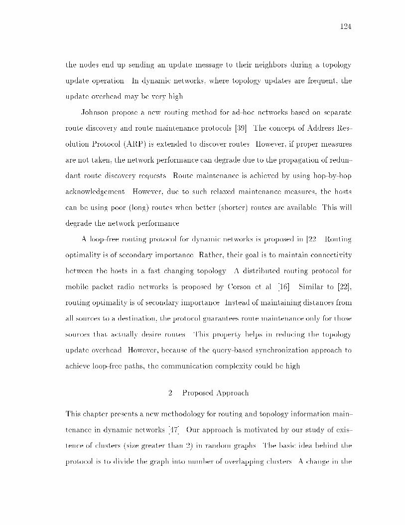
124the nodes end up sending an update message to their neighbors during a topologyupdate operation. In dynamic networks, where topology updates are frequent, theupdate overhead may be very high.Johnson propose a new routing method for ad-hoc networks based on separateroute discovery and route maintenance protocols [39]. The concept of Address Res-olution Protocol (ARP) is extended to discover routes. However, if proper measuresare not taken, the network performance can degrade due to the propagation of redun-dant route discovery requests. Route maintenance is achieved by using hop-by-hopacknowledgement. However, due to such relaxed maintenance measures, the hostscan be using poor (long) routes when better (shorter) routes are available. This willdegrade the network performance.A loop-free routing protocol for dynamic networks is proposed in [22]. Routingoptimality is of secondary importance. Rather, their goal is to maintain connectivitybetween the hosts in a fast changing topology. A distributed routing protocol formobile packet radio networks is proposed by Corson et al. [16]. Similar to [22],routing optimality is of secondary importance. Instead of maintaining distances fromall sources to a destination, the protocol guarantees route maintenance only for thosesources that actually desire routes. This property helps in reducing the topologyupdate overhead. However, because of the query-based synchronization approach toachieve loop-free paths, the communication complexity could be high.2. Proposed ApproachThis chapter presents a new methodology for routing and topology information main-tenance in dynamic networks [47]. Our approach is motivated by our study of exis-tence of clusters (size greater than 2) in random graphs. The basic idea behind theprotocol is to divide the graph into number of overlapping clusters. A change in the

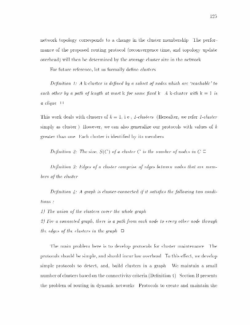
125network topology corresponds to a change in the cluster membership. The perfor-mance of the proposed routing protocol (reconvergence time, and topology updateoverhead) will then be determined by the average cluster size in the network.For future reference, let us formally de�ne clusters.De�nition 1: A k-cluster is de�ned by a subset of nodes which are `reachable' toeach other by a path of length at most k for some �xed k. A k-cluster with k = 1 isa clique. 2This work deals with clusters of k = 1, i.e., 1-clusters. (Hereafter, we refer 1-clustersimply as cluster.) However, we can also generalize our protocols with values of kgreater than one. Each cluster is identi�ed by its members.De�nition 2: The size, S(C) of a cluster C is the number of nodes in C.2De�nition 3: Edges of a cluster comprise of edges between nodes that are mem-bers of the cluster.De�nition 4: A graph is cluster-connected if it satis�es the following two condi-tions :1) The union of the clusters cover the whole graph.2) For a connected graph, there is a path from each node to every other node throughthe edges of the clusters in the graph. 2The main problem here is to develop protocols for cluster maintenance. Theprotocols should be simple, and should incur low overhead. To this e�ect, we developsimple protocols to detect, and, build clusters in a graph. We maintain a smallnumber of clusters based on the connectivity criteria (De�nition 4). Section B presentsthe problem of routing in dynamic networks. Protocols to create and maintain the

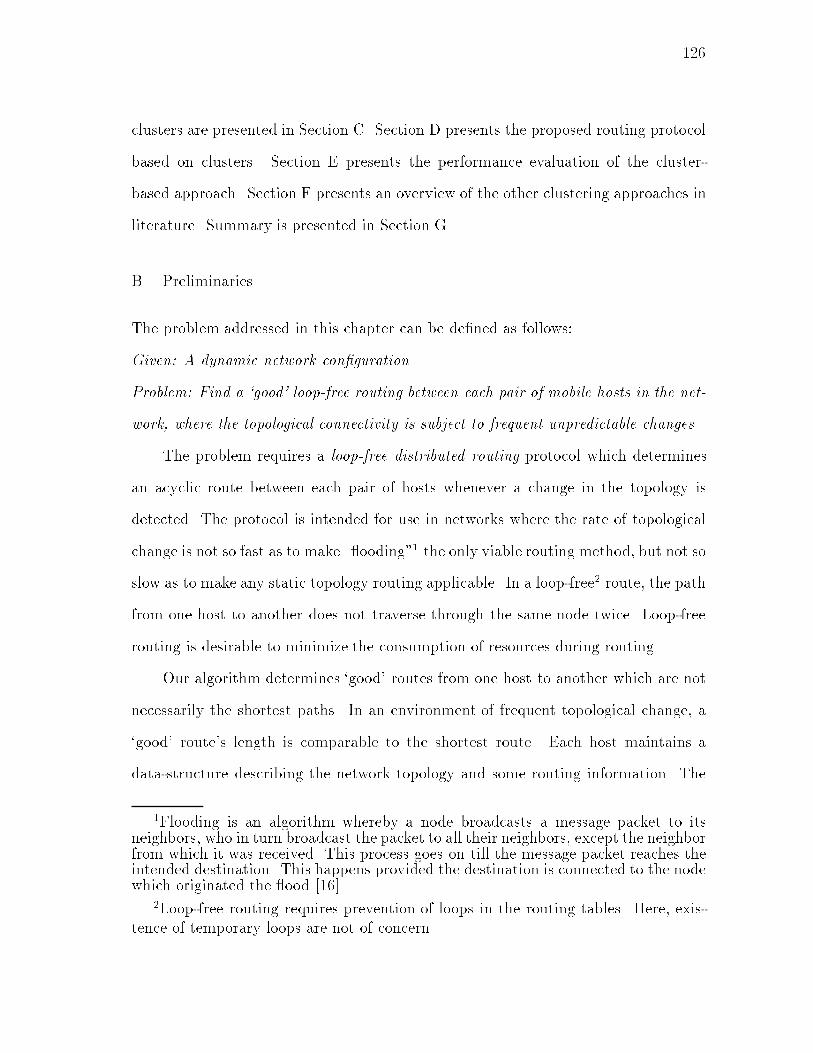
126clusters are presented in Section C. Section D presents the proposed routing protocolbased on clusters. Section E presents the performance evaluation of the cluster-based approach. Section F presents an overview of the other clustering approaches inliterature. Summary is presented in Section G.B. PreliminariesThe problem addressed in this chapter can be de�ned as follows:Given: A dynamic network con�guration.Problem: Find a `good' loop-free routing between each pair of mobile hosts in the net-work, where the topological connectivity is subject to frequent unpredictable changes.The problem requires a loop-free distributed routing protocol which determinesan acyclic route between each pair of hosts whenever a change in the topology isdetected. The protocol is intended for use in networks where the rate of topologicalchange is not so fast as to make \ ooding"1 the only viable routing method, but not soslow as to make any static topology routing applicable. In a loop-free2 route, the pathfrom one host to another does not traverse through the same node twice. Loop-freerouting is desirable to minimize the consumption of resources during routing.Our algorithm determines `good' routes from one host to another which are notnecessarily the shortest paths. In an environment of frequent topological change, a`good' route's length is comparable to the shortest route. Each host maintains adata-structure describing the network topology and some routing information. The1Flooding is an algorithm whereby a node broadcasts a message packet to itsneighbors, who in turn broadcast the packet to all their neighbors, except the neighborfrom which it was received. This process goes on till the message packet reaches theintended destination. This happens provided the destination is connected to the nodewhich originated the ood [16].2Loop-free routing requires prevention of loops in the routing tables. Here, exis-tence of temporary loops are not of concern.

127routing protocol adapts in a distributed fashion to arbitrary changes in topology inthe absence of global topological knowledge. Let an undirected graph, G = (V ,E),represent a network of mobile hosts. Each node u, in the graph denotes a mobilehost Hu. Due to the limited range of wireless transreceivers, a mobile host cancommunicate with another host only within a limited geographical region around it.This region is called the host coverage area { d being the radius. The geographicalarea covered by a host coverage area is a function of the medium used for wirelesscommunication. A host Hu is in the vicinity of Hv if the distance between nodes uand v is less than or equal to d. An edge (u,v) connects node u and node v if thecorresponding hosts are in the vicinity and have a communication link establishedbetween each other. A host may sometime be isolated where there is no other mobilehosts in its vicinity. Such a host will be represented in the graph by a disconnectednode. A host Hv1 is connected to another host Hv2 if there exists at least one pathfrom node v1 to v2.Similar to [16, 59], an underlying link-level protocol is assumed which assuresthe following:� A node is aware of all its neighbors at all times.� All packets transmitted over a link are received correctly and in proper sequencewithin a �nite time.� All control messages are processed one at a time at the nodes in the order inwhich they occur.Example B.1: The graph in Fig. 51(a) is formed based on geographical locations of 18mobile hosts. In this example, the graph is connected as each node is reachable fromevery other node. It can be observed that based on the positions, some nodes form

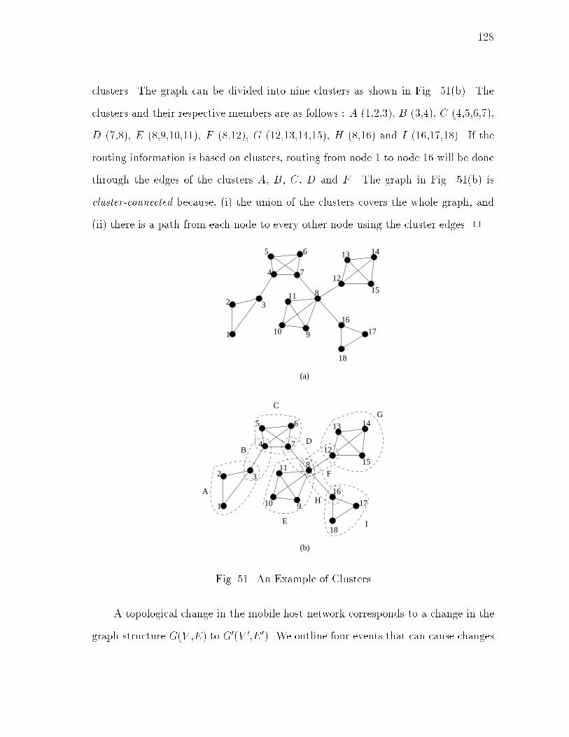
128clusters. The graph can be divided into nine clusters as shown in Fig. 51(b). Theclusters and their respective members are as follows : A (1,2,3), B (3,4), C (4,5,6,7),D (7,8), E (8,9,10,11), F (8,12), G (12,13,14,15), H (8,16) and I (16,17,18). If therouting information is based on clusters, routing from node 1 to node 16 will be donethrough the edges of the clusters A, B, C, D and F . The graph in Fig. 51(b) iscluster-connected because, (i) the union of the clusters covers the whole graph, and(ii) there is a path from each node to every other node using the cluster edges. 212

13

16

18

5 6

74

2 311 8

14

15

101 9 17

(a)

12

13

16

18

5 6

74

2 311 8

14

15

101 9 17

A

B

C

D

E

F

G

H

I

(b)Fig. 51. An Example of ClustersA topological change in the mobile host network corresponds to a change in thegraph structure G(V ,E) to G0(V 0,E0). We outline four events that can cause changes

129in the graph (in the following HA and HB are mobile hosts) :A) HA switching ON: A host HA switching ON will include itself in the graph andmake connection with all the hosts in its `vicinity'. Hence, V 0 = V [ fAg and E0 =E [ f(u;A), s.t. Hu is connected to HAg.B) HA switching OFF: A host HA switching OFF will exclude itself from the graphand delete all its edges. Hence, V 0 = V�fAg and E0 = E � f(u;A), s.t. (u;A)2Eg.C) HA gets connected to HB: Here, an edge between A and B will be added to thegraph. Hence, V 0 = V and E 0 = E [ f(A;B)g.D) HA gets disconnected from HB: Here, the edge between A and B will be removedfrom the graph. Hence, V 0 = V and E0 = E� f(A;B)g.A routing protocol will change its routing information based on the above fourtypes of changes in the graph. We now present some de�nitions and properties whichwill assist in describing the proposed routing protocol.De�nition 5: The cluster set Sn of a node n is de�ned as the set of all clustersin which n is a member. 2De�nition 6: If cluster-connectivity between any pair of nodes (n; n0) is not af-fected due to removal of a cluster C, then cluster C is redundant. 2In other words, if two nodes initially cluster-connected, are no longer cluster-connectedafter the removal of a cluster C, then cluster C is not redundant (i.e., irredundant).For example, in Fig. 51(b), there are no redundant clusters.De�nition 7: A node is a boundary node if it is a member of more than onecluster. 2In Fig. 51(b), node 3 is a boundary node as it belongs to two clusters, (1,2,3) and(3,4). However, node 1 is not a boundary node as it only belongs to (1,2,3).

130Property 1: Addition of each new node to the graph adds at least one new irre-dundant cluster. However, when the new cluster is added to the graph, the new clustermay cause one or more clusters to be redundant. 2At least one new cluster should be added to include the new node. Otherwise, thegraph will not remain cluster-connected after addition of the new node.C. Cluster FormationOur proposed routing protocol is based on the formation of clusters. Hence, e�cientcluster formation will be the crux of a routing protocol of this nature. Clustersshould be formed in such a way that the resulting graph is cluster-connected (SeeDe�nition 4). Routing from one node to another will consist of routing inside acluster and routing from cluster to cluster. A change in the dynamic network mayor may not result in a change in the cluster compositions. Here, we have assumedclusters with k = 1 (See De�nition 1). As mentioned in Section B, we have identi�edfour di�erent possible types of changes in the dynamic network graph in the occuranceof a single event. We assume that each cluster has an unique identi�er, id. Each nodemaintains a list of its neighbors, a list of clusters (Clus List) in the network, and alist of boundary nodes (Bound List) in the network. There can be multiple boundarynodes between overlapping clusters. If there are multiple boundary nodes betweenclusters, one with the biggest cluster set is chosen to be the boundary node and ismaintained in the Bound List. Note that a node can be a boundary node for morethan two overlapping clusters.In a connected network, Clus List is the same in all the nodes. It is not true ina partitioned network. This is because nodes in a partitioned network may not beaware of all the clusters in the network. Unless otherwise mentioned, the following

131discussions of the protocols consider a connected graph. Thus, unless otherwise men-tioned, all the nodes in the network have the same Clus List. We now present theprotocols for cluster updates with each type of topological change.1. Host HA Switches ONThe new graph structure G0(V 0,E0) is formed with the added node. The new node Awill result in at least one new cluster so that with the cluster, node A can route to therest of the graph. However, if A connects two disjoint subgraphs, it may result in morethan one added cluster. These new clusters are denoted by essential clusters and aredetermined by A itself. The addition of new clusters may result in zero or one or moreclusters being redundant. The two tasks performed during the topological change are(i) addition of new clusters, and (ii) removal of redundant clusters. The goal is tohave small number of clusters such that the network remains cluster-connected. Theprotocol initiated by new node A is shown in Table IV.The new node A broadcasts a message to its neighbors indicating its arrival.Upon receipt of the arrival message, the neighbors send a list of their neighbors, andClus List to A. Based on the neighbor information received from its neighbors, Adetermines the possible clusters using Create Clusters function shown in Table V,and stores them in All List. The clusters that Create Clusters function determinesdepends heavily on the order in which each node is added in the network. Thisfunction will not return the maximum clique for all the orders. This function uses a`�rst-�t' strategy to generate clusters, which does not necessarily produce maximumsized clusters. The time complexity of the Create Clusters function is O(D3).Property 2: The clusters returned by the Cluster Create function are charac-teristic of the order in which each node is added to the network. 2

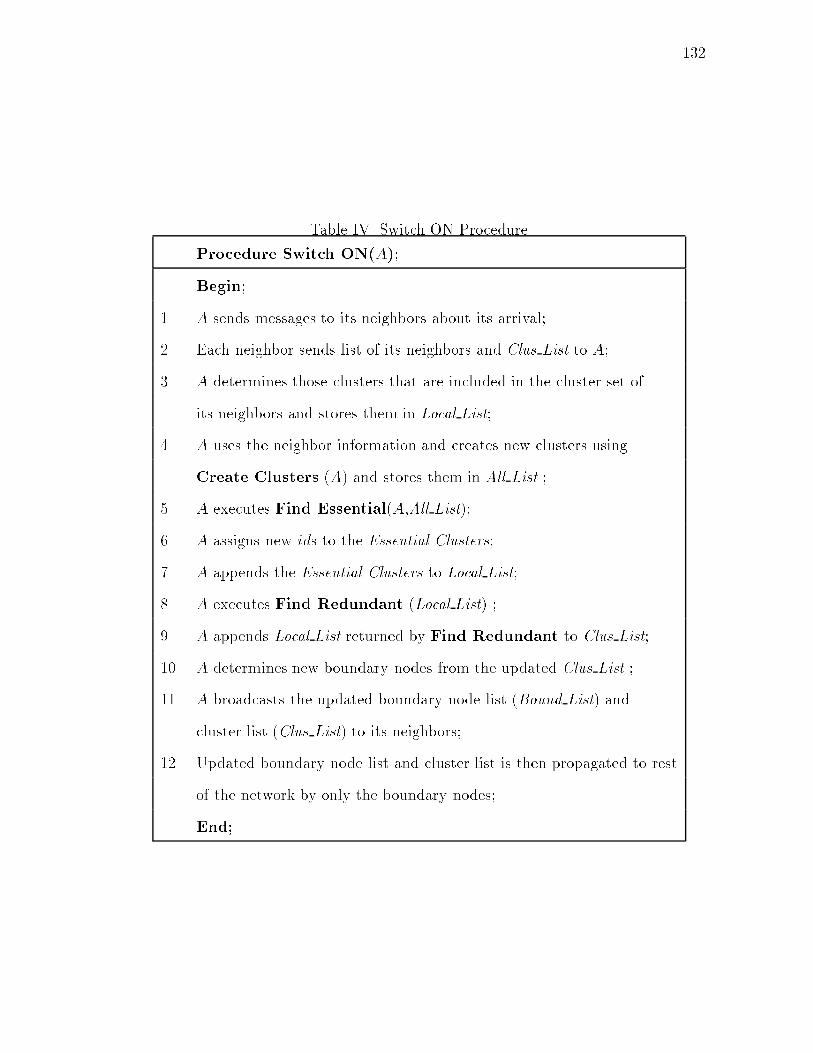
132Table IV. Switch ON ProcedureProcedure Switch ON(A);Begin;1. A sends messages to its neighbors about its arrival;2. Each neighbor sends list of its neighbors and Clus List to A;3. A determines those clusters that are included in the cluster set ofits neighbors and stores them in Local List;4. A uses the neighbor information and creates new clusters usingCreate Clusters (A) and stores them in All List ;5. A executes Find Essential(A,All List);6. A assigns new ids to the Essential Clusters;7. A appends the Essential Clusters to Local List;8. A executes Find Redundant (Local List) ;9. A appends Local List returned by Find Redundant to Clus List;10. A determines new boundary nodes from the updated Clus List ;11. A broadcasts the updated boundary node list (Bound List) andcluster list (Clus List) to its neighbors;12. Updated boundary node list and cluster list is then propagated to restof the network by only the boundary nodes;End;

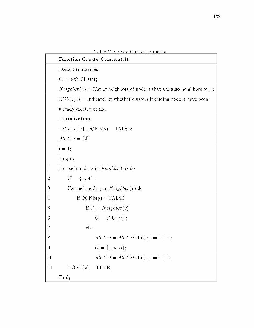
133Table V. Create Clusters FunctionFunction Create Clusters(A);Data Structures:Ci = i-th Cluster;Neighbor(n) = List of neighbors of node n that are also neighbors of A;DONE(n) = Indicator of whether clusters including node n have beenalready created or not.Initialization:1 � n � jV j, DONE(n) = FALSE;All List = f;gi = 1;Begin;1. For each node x in Neighbor(A) do2. Ci = fx;Ag ;3. For each node y in Neighbor(x) do4. if DONE(y) = FALSE5. if Ci � Neighbor(y)6. Ci = Ci [ fyg ;7. else8. All List = All List [ Ci ; i = i + 1 ;9. Ci = fx; y;Ag;10. All List = All List [ Ci ; i = i + 1 ;11. DONE(x) = TRUE ;End;

134Fig. 52 illustrates an example where di�erent node numbering (i.e., order in which anode is added to the network) leads to two di�erent set of clusters being created at thenew node (Node 6) by the Create Clusters function. One can note that a clusterof the largest size may or may not be determined by the algorithm3 presented inCreate Clusters function. However, as has been shown later, the algorithm ensuresthe connectivity of the new node with its neighbors through the clusters.1

2

5

6

4

3

1,2,3,4,61,5,61,62,3,4,63,4,63,5,73,64,65,6 1

6

4

3

1,4,6

1,5,3,6

1,2,65,3,63,4,2,64,2,62,6

5

2

(a) (b)

1,2,3,4,5,6 1,5,3,4,2,6OrderFig. 52. Di�erent Clusters Created at New Node for Di�erent Orders of Node AdditionOnce, the clusters are created using Create Clusters, the new node A thenexecutes Find Essential function shown in Table VI. The Find Essential functionsorts the clusters in All List in a non-descending order of their sizes. Initially all theclusters are marked essential. Each essential cluster C is then examined to �nd if anode (other than the new node A) in C is a member of any other essential clusters. Ifso, it marks the cluster C as non-essential. This will ensure that a node (other thanthe new node A) is a member of no more than one essential cluster. Moreover, sincethe clusters are sorted in a non-descending order of their sizes, the Find Essentialfunction returns the largest clusters possible. The essential clusters determined byFind Essential function are stored in Essential Clusters.3Finding the largest size cluster is NP-Hard [26].

135Table VI. Find Essential FunctionFunction Find Essential(A, All List);Begin;1. Sort the clusters in All List in a non-descending order of their sizes;2. For each cluster C2All List do3. Mark(C) :=essential ;4. For each cluster (C2list) ^ (Mark(C) =essential) do5. For each node (n2C) ^ (n 6= A) do6. For each cluster (C 02All List) ^ (C 0 6= C) ^ (Mark(C 0) =essential) do7. if (n2C 0)8. Mark(C) :=non-essential;9. break;10. if (Mark(C) =essential)11. Essential Clusters := Essential Clusters [ C;End;

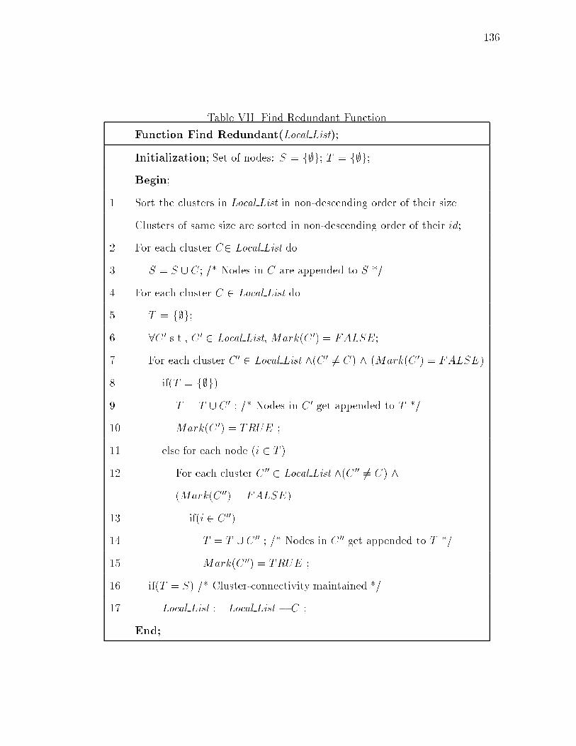
136Table VII. Find Redundant FunctionFunction Find Redundant(Local List);Initialization; Set of nodes: S = f;g; T = f;g;Begin;1. Sort the clusters in Local List in non-descending order of their size.Clusters of same size are sorted in non-descending order of their id;2. For each cluster C2 Local List do3. S = S [ C; /* Nodes in C are appended to S */4. For each cluster C 2 Local List do5. T = f;g;6. 8C 0 s.t., C 0 2 Local List, Mark(C 0) = FALSE;7. For each cluster C 0 2 Local List ^(C 0 6= C) ^ (Mark(C 0) = FALSE)8. if(T = f;g)9. T = T [ C 0 ; /* Nodes in C 0 get appended to T */10. Mark(C 0) = TRUE ;11. else for each node (i 2 T )12. For each cluster C 00 2 Local List ^(C 00 6= C) ^(Mark(C 00) = FALSE)13. if(i 2 C 00)14. T = T [ C 00 ; /* Nodes in C 00 get appended to T */15. Mark(C 00) = TRUE ;16. if(T = S) /* Cluster-connectivity maintained */17. Local List := Local List � C ;End;

137The new node A determines the new cluster ids of the essential clusters basedon the information in the cluster list (Clus List) obtained from its neighbors. Itthen appends the essential clusters to list of local clusters (Local List). The list oflocal clusters (Local List) is obtained from Clus List (Step 3 of Switch ON). Localclusters are those clusters in Clus List which are also included in the cluster set ofA's neighbors.Addition of the essential clusters may make one or more existing clusters re-dundant. The new node A then executes the Find Redundant function shown inTable VII. Node A �rst sorts the clusters in the Local List in ascending order ofsize. Clusters of same size are sorted in the order of ascending ids. The Find Re-dundant function then determines redundant clusters based on De�nition 6. Thenew cluster list is then obtained by appending the clusters remaining in Local Listafter removing the redundant clusters, to Clus List. Node A then determines thelist of boundary nodes (Bound List) from the updated Clus List. If there are mul-tiple boundary nodes between overlapping clusters, one with the biggest cluster setis chosen to be the boundary node. Node A then broadcasts the updated boundarynode list (Bound List) and cluster list Clus List to its neighbors. The neighborsthen replace their cluster list and boundary node list with the ones obtained fromA. The updated boundary node list (Bound List) and cluster list Clus List is thenpropagated to the rest of the network only by the boundary nodes.If B is the upper bound on the number of boundary nodes, and D the maximumnodal degree, the message complexity of Switch ON is O(B+D). The number ofboundary nodes, B, is upper bounded by the number of nodes in the network, N .Example C.1: For an easier understanding, Fig. 53 gives an example involving anetwork with 4 nodes. Fig. 53(a) has 4 nodes and two clusters, namely, (1,2,3)and (2,3,4). When node 5 is switched ON, it sends messages to nodes 1, 3, and

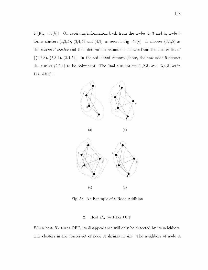
1384 (Fig. 53(b)). On receiving information back from the nodes 1, 3 and 4, node 5forms clusters (1,3,5), (3,4,5) and (4,5) as seen in Fig. 53(c). It chooses (3,4,5) asthe essential cluster and then determines redundant clusters from the cluster list off(1,2,3), (2,3,4), (3,4,5)g. In the redundant removal phase, the new node 5 detectsthe cluster (2,3,4) to be redundant. The �nal clusters are (1,2,3) and (3,4,5) as inFig. 53(d).25

1

2

3

4

5

1

2

3

4

(a) (b)

1

2

3

4

5

1

2

3

4

(c) (d)Fig. 53. An Example of a Node Addition2. Host HA Switches OFFWhen host HA turns OFF, its disappearance will only be detected by its neighbors.The clusters in the cluster-set of node A shrinks in size. The neighbors of node A

139who are cluster-mates of the shrunk cluster will `expand' the cluster. By expandinga cluster, we mean that the neighbor will determine new nodes to become a memberof that cluster. Neighbors of node A that are not cluster-mates of A will not initiateany update procedures.There could be more than one node detecting the removal of a node. SwitchOFF procedure is similar to Switch ON procedure in the sense that, there are newclusters formed and redundant clusters removed. Concurrent independent executionsof Switch OFF procedure could lead to violation of the cluster-connectivity condi-tion. We use an arbitration procedure to avoid concurrent independent executions.We require the node (neighbor of A, say, B) that is a cluster-mate of A in most num-ber of clusters, to initiate the Switch OFF procedure4. The execution of SwitchOFF procedure will expand those clusters in the cluster-set of A that node B is amember of. However, there still remains clusters in the cluster-set of A which do notcontain B. In those remaining clusters, we determine the node (say, C) that is amember of most number of clusters. This process continues till all the clusters in thecluster-set of A is covered. Unlike node B, node C will not execute Switch OFFprocedure. However, node C will just try to expand the shrunk clusters that it is partof, and not remove any redundant clusters. The new boundary list (Bound List) andthe new cluster list (Clus List) is determined by C and broadcast to its neighbors.The lists are then further propagated to the rest of the network only by the boundarynodes.The procedure initiated by node B is shown in Table VIII. Let us illustrate itwith an example.Example C.2: Fig. 54 shows the cluster formations when a node is turned OFF in4If there are multiple such nodes, we use a tie-breaking test; e.g., node with thelarger identifier.

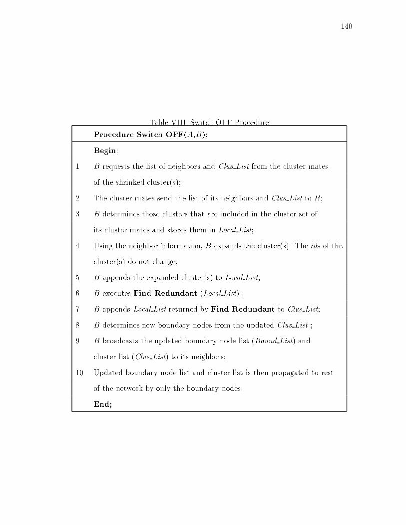
140Table VIII. Switch OFF ProcedureProcedure Switch OFF(A,B);Begin;1. B requests the list of neighbors and Clus List from the cluster matesof the shrinked cluster(s);2. The cluster mates send the list of its neighbors and Clus List to B;3. B determines those clusters that are included in the cluster set ofits cluster mates and stores them in Local List;4. Using the neighbor information, B expands the cluster(s). The ids of thecluster(s) do not change;5. B appends the expanded cluster(s) to Local List;6. B executes Find Redundant (Local List) ;7. B appends Local List returned by Find Redundant to Clus List;8. B determines new boundary nodes from the updated Clus List ;9. B broadcasts the updated boundary node list (Bound List) andcluster list (Clus List) to its neighbors;10. Updated boundary node list and cluster list is then propagated to restof the network by only the boundary nodes;End;

141a network. Fig. 54(a) has six nodes with three clusters, namely, (1,2,3), (2,3,4) and(4,5,6). When node 6 is turned OFF, the cluster (4,5,6) shrinks to (4,5) (Fig. 54(b)).Node 4 and 5 detect node 6 switching OFF. Since, node 5 has the higher identi�er,it initiates the Switch OFF procedure. Node 5 gets neighbor information and thecluster list from 3 and 4. It then expands the cluster (4,5) to (3,4,5) (Fig. 54(c)).Node 5 now has f(1,2,3), (2,3,4), (3,4,5)g in the cluster list. In the redundant removalphase, node 5 detects the cluster (2,3,4) to be redundant. The �nal clusters are (1,2,3)and (3,4,5) as in Fig. 54(d). 21

2

3

4

1

2

3

4

5

6

1

2

3

4

5

1

2

3

4

55

(a) (b)

(d)(c)Fig. 54. An Example of a Node RemovalThe message complexity of Switch OFF is also O(B+D), where, B is the upperbound on the number of boundary nodes, and D the maximum nodal degree. Asstated earlier, the number of boundary nodes, B, is upper bounded by the number of

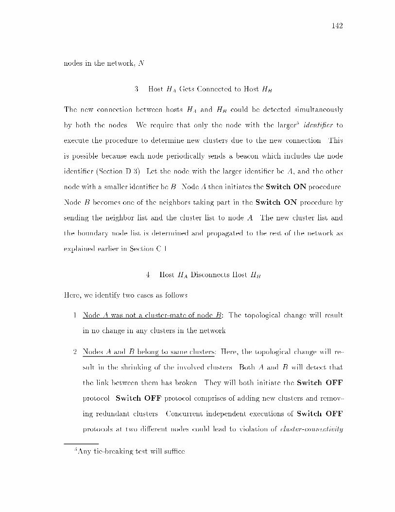
142nodes in the network, N .3. Host HA Gets Connected to Host HBThe new connection between hosts HA and HB could be detected simultaneouslyby both the nodes. We require that only the node with the larger5 identi�er toexecute the procedure to determine new clusters due to the new connection. Thisis possible because each node periodically sends a beacon which includes the nodeidenti�er (Section D.3). Let the node with the larger identi�er be A, and the othernode with a smaller identi�er be B. Node A then initiates the Switch ON procedure.Node B becomes one of the neighbors taking part in the Switch ON procedure bysending the neighbor list and the cluster list to node A. The new cluster list andthe boundary node list is determined and propagated to the rest of the network asexplained earlier in Section C.1.4. Host HA Disconnects Host HBHere, we identify two cases as follows.1. Node A was not a cluster-mate of node B: The topological change will resultin no change in any clusters in the network.2. Nodes A and B belong to same clusters: Here, the topological change will re-sult in the shrinking of the involved clusters. Both A and B will detect thatthe link between them has broken. They will both initiate the Switch OFFprotocol. Switch OFF protocol comprises of adding new clusters and remov-ing redundant clusters. Concurrent independent executions of Switch OFFprotocols at two di�erent nodes could lead to violation of cluster-connectivity5Any tie-breaking test will su�ce.

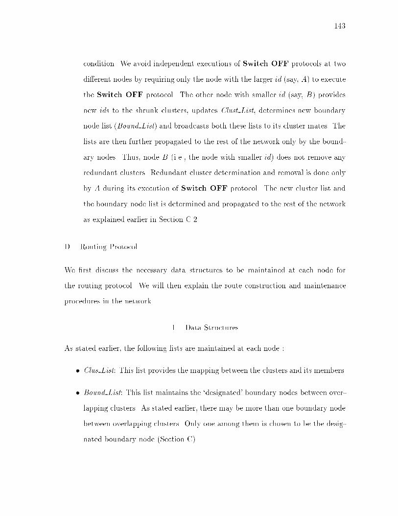
143condition. We avoid independent executions of Switch OFF protocols at twodi�erent nodes by requiring only the node with the larger id (say, A) to executethe Switch OFF protocol. The other node with smaller id (say, B) providesnew ids to the shrunk clusters, updates Clust List, determines new boundarynode list (Bound List) and broadcasts both these lists to its cluster mates. Thelists are then further propagated to the rest of the network only by the bound-ary nodes. Thus, node B (i.e., the node with smaller id) does not remove anyredundant clusters. Redundant cluster determination and removal is done onlyby A during its execution of Switch OFF protocol. The new cluster list andthe boundary node list is determined and propagated to the rest of the networkas explained earlier in Section C.2.D. Routing ProtocolWe �rst discuss the necessary data structures to be maintained at each node forthe routing protocol. We will then explain the route construction and maintenanceprocedures in the network. 1. Data StructuresAs stated earlier, the following lists are maintained at each node :� Clus List: This list provides the mapping between the clusters and its members.� Bound List: This list maintains the `designated' boundary nodes between over-lapping clusters. As stated earlier, there may be more than one boundary nodebetween overlapping clusters. Only one among them is chosen to be the desig-nated boundary node (Section C).

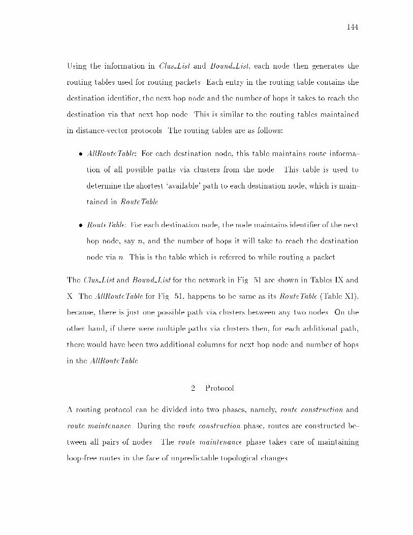
144Using the information in Clus List and Bound List, each node then generates therouting tables used for routing packets. Each entry in the routing table contains thedestination identi�er, the next hop node and the number of hops it takes to reach thedestination via that next hop node. This is similar to the routing tables maintainedin distance-vector protocols. The routing tables are as follows:� AllRouteTable: For each destination node, this table maintains route informa-tion of all possible paths via clusters from the node. This table is used todetermine the shortest `available' path to each destination node, which is main-tained in RouteTable.� RouteTable: For each destination node, the node maintains identi�er of the nexthop node, say n, and the number of hops it will take to reach the destinationnode via n. This is the table which is referred to while routing a packet.The Clus List and Bound List for the network in Fig. 51 are shown in Tables IX andX. The AllRouteTable for Fig. 51, happens to be same as its RouteTable (Table XI),because, there is just one possible path via clusters between any two nodes. On theother hand, if there were multiple paths via clusters then, for each additional path,there would have been two additional columns for next hop node and number of hopsin the AllRouteTable. 2. ProtocolA routing protocol can be divided into two phases, namely, route construction androute maintenance. During the route construction phase, routes are constructed be-tween all pairs of nodes. The route maintenance phase takes care of maintainingloop-free routes in the face of unpredictable topological changes.

145Table IX. Clus List at Each NodeClusterId NodesA 1,2,3B 3,4C 4,5,6,7D 7,8E 8,9,10,11F 8,12G 12,13,14,15H 8,16I 16,17,18Table X. Bound List at Each NodeClusterIds NodeA,B 3B,C 4C,D 7D,E,F,H 8F,G 12H,I 8,16

146Table XI. RouteTable at Node 6, Cluster CDestNode NextHop Hops1 4 32 4 33 4 24 - 15 - 16 - 07 - 18 7 29 7 310 7 311 7 312 7 313 7 414 7 415 7 416 7 317 7 418 7 4

147a. Route Construction PhaseThe protocols to maintain clusters in the face of various network events have beenexplained earlier. Upon receipt of new cluster information, a boundary node storesthe new cluster list in its Clus List, the new boundary list in its Bound List, and thenrebroadcasts the information. A boundary node has to forward the new informationonly once. Nodes other than the boundary nodes listen to this information andjust update their tables. In this manner, the information of each network event isdistributed to all the nodes. Each node now has the topology information of thewhole network. Based on the information in Clus List and Bound List, each nodethen generates the RouteTable and AllRouteTable.Each message packet contains the identi�er of the destination node in its header.When a node receives a message packet, it looks up the RouteTable to determinethe next hop node for the packet's destination. The node then forwards the messagepacket to the next hop node. This process of forwarding continues till the packetreaches its destination.b. Route Maintenance PhaseThis phase begins when there is a change in the network topology (host connec-tion/disconnection, link failure/recovery). The route maintenance in our approachbasically boils down to cluster maintenance. The protocols for cluster maintenancehave been explained previously. After a change in topology, all the nodes have thecomplete topology information in the form of cluster list (Clus List) and boundarynode list (Bound List). If all the nodes have a consistent view of the topology, routingloops are not formed. However, due to long propagation delays, partitioned network,etc., some nodes may have inconsistent topology information. This might lead to

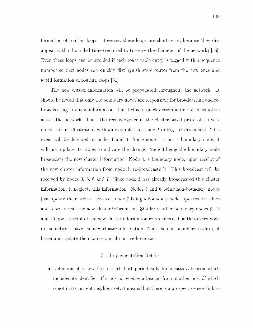
148formation of routing loops. However, these loops are short-term, because they dis-appear within bounded time (required to traverse the diameter of the network) [56].Even these loops can be avoided if each route table entry is tagged with a sequencenumber so that nodes can quickly distinguish stale routes from the new ones andavoid formation of routing loops [61].The new cluster information will be propagated throughout the network. Itshould be noted that only the boundary nodes are responsible for broadcasting and re-broadcasting any new information. This helps in quick dissemination of informationacross the network. Thus, the reconvergence of the cluster-based protocols is veryquick. Let us illustrate it with an example. Let node 2 in Fig. 51 disconnect. Thisevent will be detected by nodes 1 and 3. Since node 1 is not a boundary node, itwill just update its tables to indicate the change. Node 3 being the boundary nodebroadcasts the new cluster information. Node 4, a boundary node, upon receipt ofthe new cluster information from node 3, re-broadcasts it. This broadcast will bereceived by nodes 3, 5, 6 and 7. Since node 3 has already broadcasted this clusterinformation, it neglects this information. Nodes 5 and 6 being non-boundary nodesjust update their tables. However, node 7 being a boundary node, updates its tablesand rebroadcasts the new cluster information. Similarly, other boundary nodes 8, 12and 16 upon receipt of the new cluster information re-broadcast it so that every nodein the network have the new cluster information. And, the non-boundary nodes justlisten and update their tables and do not re-broadcast.3. Implementation Details� Detection of a new link : Each host periodically broadcasts a beacon whichincludes its identi�er. If a host h receives a beacon from another host h0 whichis not in its current neighbor set, it means that there is a prospective new link to

149h

h’

h’Fig. 55. Movements That Cause Unnecessary Link Creations/Deletionsbe created. However, the Switch ON procedure is not immediately initiated.Only after a certain number of successive beacons is received from the same hostis the Switch ON procedure initiated. This is to avoid unnecessary oscillationsdue to the host h0 moving in and out of host h's vicinity. Fig. 55 shows thescenarios where the movement of h0 could cause a sequence of unnecessary linkcreations/deletions.� Detection of a link break : If a host h does not receive a certain number of con-secutive beacons from its neighbor h0, it will assume that either h0 has moved outof its vicinity or that h0 is disconnected. Host h will then follow the procedurefor host disappearance as explained in Section C.2.E. Performance Evaluation 1. ComplexityThis section compares the cluster-based approach's worst-case performance with theperformance of Distributed Bellman-Ford (DBF) [11], Ideal Link State (ILS) [25], Dif-fusing Update Algorithm (DUAL) [25], NP [16] and ooding. The ILS protocol [25]requires that each topology change be transmitted to every node. The DUAL pro-tocol [25] is a distance-vector loop-free algorithm based on internodal coordinationspanning multiple hops. DUAL is known to be the lowest complexity distance-vector

150algorithm. NP protocol [16] is source-initiated routing protocol that provides loop-free routing only to desired destinations in a dynamic network. Flooding does nothave any control overhead due to topology updates/maintenance. Everytime a nodewants to send a packet to a destination, the node broadcasts the packet to its neigh-bors, who in turn broadcast the packet to all their neighbors, except the neighborfrom which it was received. This process goes on till the message packet reaches theintended destination.The performance metrics are the time complexity (TC) and the communicationcomplexity (CC) [25]. Time complexity is de�ned as the number of steps requiredfor the network to reconverge after a topology change. The number of messagesrequired to accomplish the reconvergence is called the communication complexity.The assumptions made while making the comparisons are same as in [25]. They areas follows:� The routing algorithm behaves synchronously, so that every host in the networkexecutes a step of the algorithm simultaneously at �xed points in time.� At each step, the host receives and processes all the inputs originated duringthe preceding step and, if required, sends update messages at the same step.We borrow the complexity computations of DBF, ILS, and DUAL from [25].Table XII lists the protocols with the complexities. The complexity parameters areas follows:� N: Number of nodes in the network.� E: Number of links in the network.� d: Diameter of the network. The diameter of a network is de�ned as the lengthof the longest shortest path in hops between any two nodes [25].

151� D: Maximum degree of a node.� B: Upper bound on the number of unique boundary nodes in the network.Overlapping clusters may have more than one boundary node between them.However, only one of them will be considered as the boundary node and willbe used to pass messages between clusters. The other boundary nodes areconsidered as non-boundary nodes. The procedure to select a boundary nodehas been described in Section C.� x: Number of nodes a�ected by the topological change.� l: Diameter of the a�ected network segment.Table XII. Complexity ComparisonProtocol TC CCDBF [11] O(N) O(N2)ILS [25] O(d) O(E)DUAL [25] O(x) O(Dx)NP [16] O(l) O(x)Cluster O(d) O(B +D)Flooding 0 0Since, ooding does not have any topology update overhead, the time complexityand communication complexity of ooding is zero. The complexities of DUAL andNP will be high if x � N (This is true in the situations when a node fails or switcheso�.), i.e., when most of the nodes in the network are a�ected by the topologicalchange. In such cases, the diameter of the a�ected segment, l � d. The perfor-

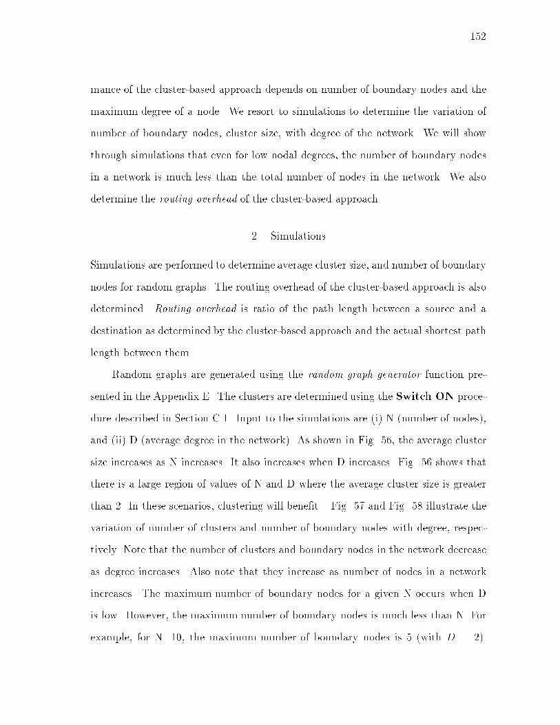
152mance of the cluster-based approach depends on number of boundary nodes and themaximum degree of a node. We resort to simulations to determine the variation ofnumber of boundary nodes, cluster size, with degree of the network. We will showthrough simulations that even for low nodal degrees, the number of boundary nodesin a network is much less than the total number of nodes in the network. We alsodetermine the routing overhead of the cluster-based approach.2. SimulationsSimulations are performed to determine average cluster size, and number of boundarynodes for random graphs. The routing overhead of the cluster-based approach is alsodetermined. Routing overhead is ratio of the path length between a source and adestination as determined by the cluster-based approach and the actual shortest pathlength between them.Random graphs are generated using the random graph generator function pre-sented in the Appendix E. The clusters are determined using the Switch ON proce-dure described in Section C.1. Input to the simulations are (i) N (number of nodes),and (ii) D (average degree in the network). As shown in Fig. 56, the average clustersize increases as N increases. It also increases when D increases. Fig. 56 shows thatthere is a large region of values of N and D where the average cluster size is greaterthan 2. In these scenarios, clustering will bene�t. Fig. 57 and Fig. 58 illustrate thevariation of number of clusters and number of boundary nodes with degree, respec-tively. Note that the number of clusters and boundary nodes in the network decreaseas degree increases. Also note that they increase as number of nodes in a networkincreases. The maximum number of boundary nodes for a given N occurs when Dis low. However, the maximum number of boundary nodes is much less than N. Forexample, for N=10, the maximum number of boundary nodes is 5 (with D = 2).

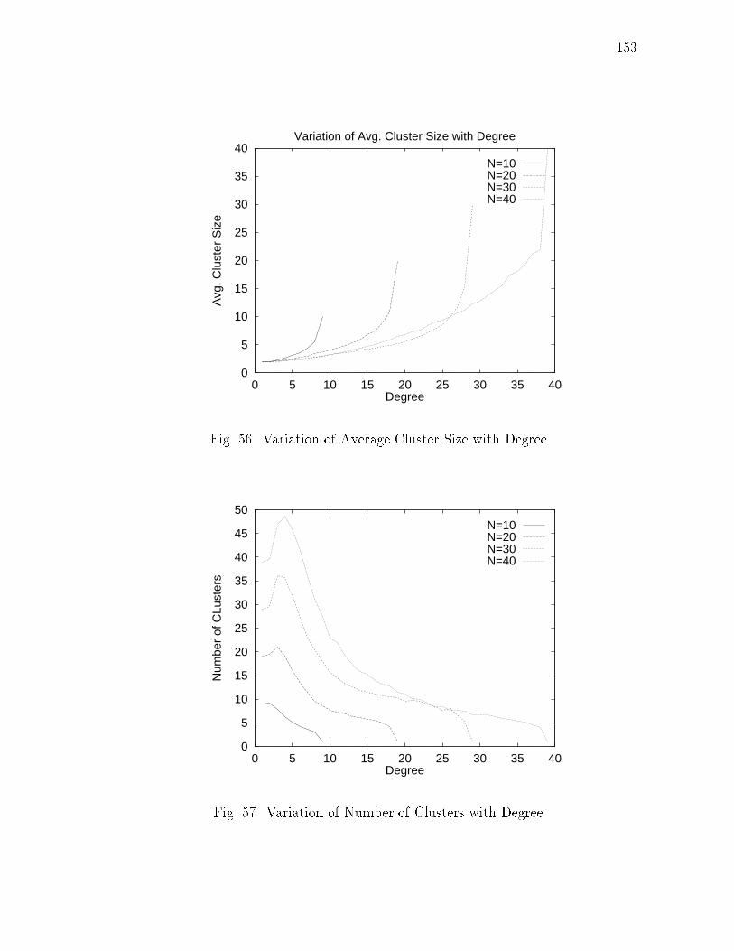
1530

5

10

15

20

25

30

35

40

0 5 10 15 20 25 30 35 40

Avg

. Clu

ster

Siz

e

Degree

Variation of Avg. Cluster Size with Degree

N=10N=20N=30N=40

Fig. 56. Variation of Average Cluster Size with Degree0

5

10

15

20

25

30

35

40

45

50

0 5 10 15 20 25 30 35 40

Num

ber

of C

Lust

ers

Degree

N=10N=20N=30N=40

Fig. 57. Variation of Number of Clusters with Degree

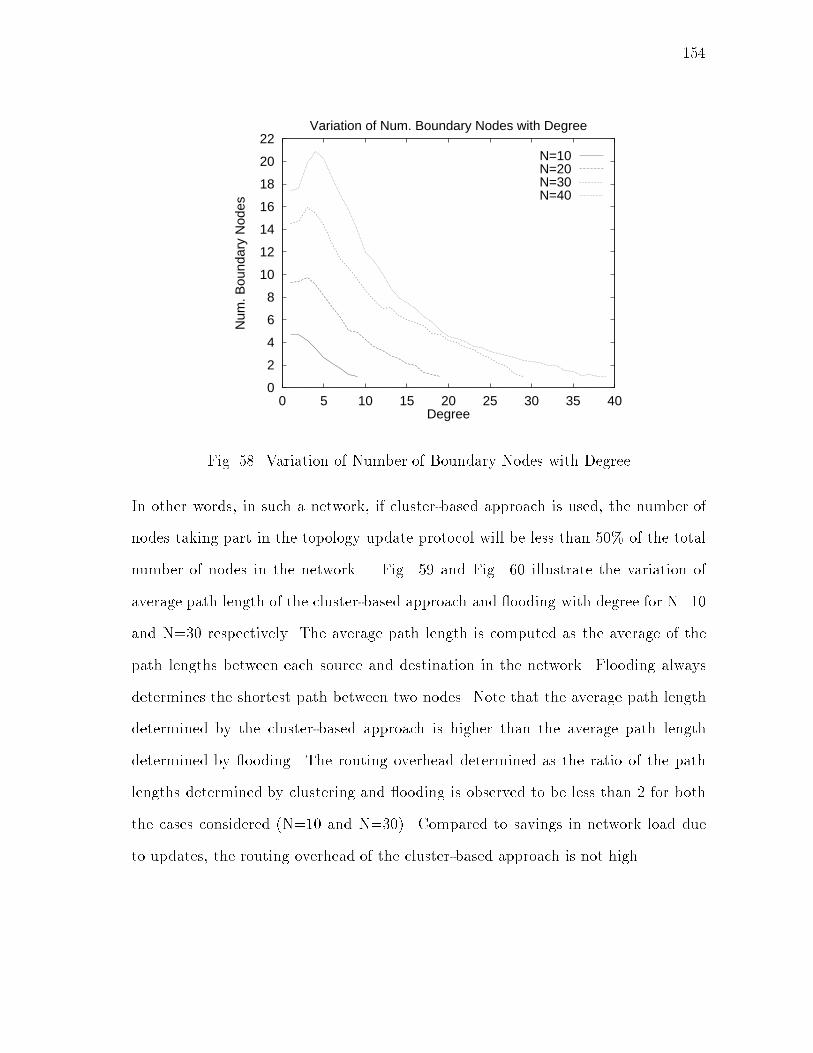
1540

2

4

6

8

10

12

14

16

18

20

22

0 5 10 15 20 25 30 35 40

Num

. Bou

ndar

y N

odes

Degree

Variation of Num. Boundary Nodes with Degree

N=10N=20N=30N=40

Fig. 58. Variation of Number of Boundary Nodes with DegreeIn other words, in such a network, if cluster-based approach is used, the number ofnodes taking part in the topology update protocol will be less than 50% of the totalnumber of nodes in the network. Fig. 59 and Fig. 60 illustrate the variation ofaverage path length of the cluster-based approach and ooding with degree for N=10and N=30 respectively. The average path length is computed as the average of thepath lengths between each source and destination in the network. Flooding alwaysdetermines the shortest path between two nodes. Note that the average path lengthdetermined by the cluster-based approach is higher than the average path lengthdetermined by ooding. The routing overhead determined as the ratio of the pathlengths determined by clustering and ooding is observed to be less than 2 for boththe cases considered (N=10 and N=30). Compared to savings in network load dueto updates, the routing overhead of the cluster-based approach is not high.

1551

1.2

1.4

1.6

1.8

2

2.2

2.4

2.6

2.8

3

1 2 3 4 5 6 7 8 9

Ave

rage

Pat

h Le

ngth

Degree

ClusterFlooding

Fig. 59. Variation of Average Path Length with Degree: N=101

1.5

2

2.5

3

3.5

4

4.5

5

5.5

6

0 5 10 15 20 25 30

Ave

rage

Pat

h Le

ngth

Degree

ClusterFlooding

Fig. 60. Variation of Average Path Length with Degree: N=30

156F. Other Clustering ApproachesThe problem of clustering in networks has been discussed earlier in literature [23, 34,41, 66, 70]. Our work di�ers from the earlier works in the following respect:� Clustering was proposed as a hierarchical approach in earlier literature to re-duce the amount of routing information stored at individual hosts. The entirenetwork is thought of as a tree of hierarchies, in which each node at a higherlevel is made up of one or more nodes from lower levels. Each host has to takepart in two updating procedures: one local within its cluster, and the otherglobal with other distant nodes. In this paper, clustering is restricted to a sin-gle level. The main advantage behind using cluster-based approaches is that theway we maintain the clusters, which, limits the number of nodes taking partin the topology-update operation, thereby, reducing the network load duringtopology updates.� The cluster creation and maintenance algorithms have not been discussed inmost of the literature where if it is discussed, it either is speci�cally for regulargraph structures [41, 70], or employs a cluster controller (or leader) [66]. Inthis work we create and maintain a small number of clusters (cliques) in anarbitrary graph. The cluster graph is created using a sequence of Switch ONprocedures (one procedure call for each node being added). The cluster ismaintained in the face of di�erent network events by calling the appropriatealgorithms as explained in this work.� Cluster overlapping in some approaches requires each node to be included inmore than one cluster [66, 70]. However, in this work we do not require all thenodes to be included in more than one cluster.

157� Unlike the previous approaches, we require our clustering algorithms to cre-ate and maintain clusters such that they satisfy the cluster-connectivity crite-rion (De�nition 4). Since, we require the network to be cluster-connected, wecan apply any routing protocol directly by just replacing the nodes by clusters.Thus, we can enjoy the advantages of a chosen routing protocol (loop-free routes,etc.), and also the cluster-based approach (low topology update overhead, etc.).G. SummaryProposed in this chapter is a new methodology for routing in mobile wireless networks.Simple distributed algorithms are proposed for cluster creation and maintenance.This chapter shows that routing protocols based on clusters could obtain performanceimprovements over previous approaches. Cluster-based protocols allow the networkto enjoy the liberty of maintaining routes between all pairs of nodes at all times,without causing much network overhead. Thus, a compromise on routing optimalityas suggested in [16] to avoid network congestion might not be required.Quick reconvergence in some protocols like DSDV [61] is obtained by quick re-broadcast by each and every recipient of the broadcast, causing degradation of theavailability of the wireless medium. However, in our approach, re-broadcast is doneonly by the boundary nodes. Nodes other than boundary nodes just listen and updatetheir tables.Similar to [16, 22] the cluster-based approach does not guarantee shortest path.This is due to the fact that the clusters are created using the �rst-�t approach, whichdoes not produce the maximum clusters in the graph. However, it has been shownthat the routing overhead of the cluster-based approach is not high.

158CHAPTER VICONCLUSIONThis chapter contains a summary of results presented in this dissertation, followedby suggestions for future work.A. Summary of ResultsWe classify the mobile wireless networks into infrastructure networks and dynamicnetworks. Infrastructure networks are typically two-tiered network composing of astatic backbone network and a peripheral wireless network. Dynamic networks on theother hand comprises of only mobile hosts that communicate with one another usingwireless links. This dissertation studies the following performance issues in mobilewireless networks { recovery issues in infrastructure networks, location managementissues in infrastructure networks, and routing in dynamic networks.Mobility of users and limited wireless bandwidth bring forth interesting dimen-sions into design of recovery protocols in a mobile wireless networks. Work in thisdissertation is the �rst e�ort to study the e�ect of mobility and wirelessness on the de-sign and performance of recovery protocols. Presented in this dissertation are recoveryschemes for a mobile wireless environment. The recovery schemes are a combinationof a state-saving and a hando� scheme. Each combination provides some level ofavailability and requires some amount of resources: network bandwidth, memory,and processing power. A fundamental relationship between the performance of re-covery schemes, failure rate, mobility and wireless bandwidth is established. Throughanalysis, it is shown that there can be no single recovery scheme that performs wellfor all mobile environments. However, we determine the optimal recovery schemefor each environment, where an environment is determined by the mobility, wireless

159bandwidth and the failure rate.Location management is one of the most important issues in infrastructure mobilewireless networks. In order to communicate with an user, one needs to know theuser's location. Thus, the network faces a problem of continuously keeping trackof the location of each and every user. This problem becomes noticeable when thenetwork sizes are large. This dissertation presents centralized and distributed locationmanagement schemes.Centralized schemes like IS-41 use home location servers for location manage-ment. The location management schemes in IS-41 are ine�cient because they incur avery heavy load on the network and the home location servers due to location updatesand searches. Forwarding technique is used to lower the network load due to updatesin the network and at the home location servers due to user mobility. However, for-warding increases the search cost (call set-up time). Two heuristics are presentedto limit the search cost. A search-update (caching) strategy is presented to furtherreduce the search cost and also the call-delivery rate at the home location server. Theperformance of the schemes depend on (i) call-mobility pattern of the user, and (ii)cost of forwarding. Analytical models are built to compare the performance of theproposed schemes with the IS-41 scheme. It is determined that the proposed schemesperform signi�cantly better than the IS-41 scheme for most call-mobility patterns andforwarding costs. Although bene�cial, forwarding and search-updates complicate themaintenance, and fault-tolerance issues. To overcome these problems, this disserta-tion also presents cost-e�ective techniques for fault tolerance and forwarding pointermaintenance.The bottleneck in the centralized schemes are the home location servers. Insteadof a home location server, a hierarchy of location servers is proposed for locationmanagement. The signalling load is now distributed over various location servers. A

160suite of location management schemes for such a network architecture is presented.Each scheme is a combination of a search strategy, update strategy and a search-update strategy. A static location management scheme requires a single combinationto be executing always. It is observed that there is no combination that outperformedothers for all call-mobility patterns. Since, the user behavior (call-mobility pattern)is not always available to the system designer, there is need for adaptive locationmanagement. An adaptive scheme is presented that is based on the assumption thatthe past history of the system re ects the behavior in the future. Results indicatethat the adaptive scheme performs better than the static scheme for a wide range ofcall-mobility patterns.The conventional routing protocols were not designed for dynamic networks (e.g.,ad-hoc networks, packet radio networks) where the topological connectivity is subjectto frequent, unpredictable change. In addition to host and link failures, changes intopology can occur due to host mobility and disconnections. Due to limited band-width available on the wireless links, the amount of information exchanged or prop-agated during topology updates has to be kept low in such networks. To achievethis goal, we propose a cluster-based methodology for routing in dynamic networks.The basic idea behind the protocol is to divide the graph into number of overlap-ping clusters. The main advantage of our approach is that it limits the number ofnodes taking part in the topology-update operation, thereby, reducing the networkload during topology updates. We propose simple protocols for cluster creation andmaintenance. Compared to existing and conventional routing protocols, the proposedcluster-based approach incurs lower overhead during topology updates and also pro-vides quicker reconvergence. Although, the cluster-based approach does not guarantee

161shortest path, it is determined using simulations that the routing overhead1 of thecluster-based approach is small.B. Future WorkThe �eld of mobile computing is still relatively new. There are many challenging andinteresting areas of future research that can stem out of the work presented in thisdissertation. The following presents a summary.Chapter II dealt with application-level recovery protocols in a mobile environ-ment. An opportunity for further research exists in other fault-tolerance issues inmobile computing, such as recovery from failure of a base station, fault-tolerant broad-cast/multicast protocols, and development of new and e�cient distributed recoveryschemes. Although, the analysis presented in this research is used to analyze recov-ery protocols, we feel that this analytical framework could also be used with somevariations to analyze the e�ect of mobility, wireless bandwidth and disconnections onthe performance of �le systems, and database systems.Chapter III presented schemes to improve the performance of location manage-ment schemes in a personal communication network. Chapter IV presented locationmanagement schemes for a network comprising of a hierarchy of location servers.The schemes were analyzed using analytical modeling or simulations. It would beinteresting to determine the performance of these schemes using real call-mobilitytraces. Secondly, in this work we did not consider variance in the call set-up times.From a user's perspective, apart from the mean call set-up time, the variance is alsoa key parameter. Future work should involve development of schemes that reduce1Routing overhead is ratio of the path length between the source and the destina-tion as determined by the cluster-based approach and the actual shortest path lengthbetween them.

162the variance. It was shown in Chapter IV that a simple adaptive scheme performsbetter than static schemes for non-uniform call-mobility patterns. A potential area ofresearch is to study other sophisticated adaptive location management schemes thatis able to better predict user behavior.A cluster-based approach for routing in dynamic networks was presented in Chap-ter V. Protocols for cluster creation and maintenance were presented. A number ofdi�erent issues remain to be studied: (a) Extensions of these protocols to supportconcurrent events. (b) Load balancing among multiple boundary nodes. In our work,there is only one unique boundary node selected between any two clusters for propa-gating update information. (c) Algorithms to create and maintain clusters such thatthere is always more than one boundary node between any two overlapping clus-ters. This will add robustness during a boundary node failure. (d) Generalizationof 1-clusters to k-clusters (where k > 1). This will require design of more complexalgorithms for cluster creation and maintenance. The interesting issue will be todetermine if there is any performance improvement using k-clusters (where k > 1)instead of 1-clusters.

163REFERENCES[1] A. Acharya, B. R. Badrinath, \Checkpointing Distributed Applications on MobileComputers," Proc. International Conference on Parallel and Distributed Informa-tion Systems, Austin, Texas, pp. 73-80, September, 1994.[2] S. Alagar, R. Rajagopalan, S. Venkatesan, \Tolerating mobile support station fail-ures," Proc. IEEE Conference on Fault Tolerant Systems, pp. 225-231, December,1995.[3] R. Alonso, H. Korth, \Database System Issues in Nomadic Computing," Proc.ACM SIGMOD International Conference on Management of Data, pp. 388-392,May, 1993.[4] B. Awerbuch, D. Peleg, \Concurrent Online Tracking of Mobile Users," Proc.ACM SIGCOMM Symposium on Communication, Architectures and Protocols,Zurich, Switzerland, pp. 221-233, September, 1991.[5] B. R. Badrinath, T. Imielinski, A. Virmani, \Locating Strategies for PersonalCommunication Networks," Proc. IEEE GLOBECOM Workshop on Networkingof Personal Communication, December 1992.[6] A. Bakre, B. R. Badrinath, \I-TCP: Indirect TCP for Mobile Hosts," Proc. In-ternational Conference on Distributed Computing Systems, Oct., 1994.[7] B. Bakshi, P. Krishna, N. H. Vaidya, D. K. Pradhan, \Improving Performanceof TCP over Wireless Networks," Technical Report # TR-96-014, Department ofComputer Science, Texas A&M University, May, 1996.

164[8] H. Balakrishnan, S. Seshan, E. Amir, R. H. Katz, \Improving TCP/IP Perfor-mance over Wireless Networks," Proc. ACM Conference on Mobile Computingand Networking, pp. 2-11, November 1995.[9] D. M. Balston, R. C. V. Macario, Cellular Radio Systems, Artech House, Boston,Massachusetts, 1994.[10] Amotz Bar-Noy, H. Kessler, \Tracking Mobile Users in Wireless CommunicationNetworks," Proc. IEEE, INFOCOM, pp. 1232-1239, May, 1993.[11] D. Bertsekas, R. Gallager, Data Networks, Second Edition, Prentice Hall Inc.,Englewood Cli�s, New Jersey, 1992.[12] Pravin Bhagwat, Charles. E. Perkins, \A Mobile Networking System Basedon Internet Protocol (IP)," Proc. USENIX Symposium on Mobile and Location-Independent Computing, pp. 69-82, August 1993.[13] A. Borg, J. Baumbach, S. Glazer, \A Message System Supporting Fault-tolerance," Proc. Ninth ACM Symposium of Operating Systems and Principles,pp. 90-99, October, 1983.[14] R. Caceres, L. Iftode, \Improving the Performance of Reliable Transport Pro-tocols in Mobile Computing Environments," IEEE Journal on Selected Areas inCommunications, Vol. 13, No. 5, Oct., 1994.[15] Cellular Digital Packet Data System Speci�cation: Release 1.1, CDPD Fo-rum Inc., January, 1995. (Contact CDPD Forum Executive Director, email:info@forum.cdpd.net)[16] M. Scott Corson, A. Ephremides, \A Distributed Routing Algorithm for MobileWireless Networks," ACM Journal on Wireless Networks, Vol.1, No.1, pp. 61-81,

1651995.[17] W. Diepstraten, G. Ennis, P. Bellanger, \DFWMAC - Distributed FoundationWireless Medium Access Control," IEEE Document P802.11-93/190, Nov., 1993.(Contact Wim Diepstraten, email: Wim.Diepstraten@utrecht.ncr.com)[18] E. W. Dijkstra, \Self-Stabilizing Systems in Spite of Distributed Control," Com-munications of the ACM, Vol.17, No.11, pp. 643-644, 1974.[19] S. Dolev, D. K. Pradhan, J. L. Welch, \Modi�ed Tree Structure for LocationManagement in Mobile Environments," Proc. IEEE INFOCOM, pp. 530-537,May, 1995.[20] G. H. Forman, J. Zahorjan, \The Challenges of Mobile Computing," IEEE Com-puter, Vol. 27, No. 4, pp. 38-47, April, 1994.[21] R. J. Fowler, \The Complexity of Using Forwarding Address for DecentralizedObject Finding," Proc. ACM Symposium on Principles of Distributed Computing,pp. 108-120, 1986.[22] E. Gafni, D. P. Bertsekas, \Distributed Algorithms for Generating Loop-freeRoutes with Frequently Changing Topology," IEEE Transactions on Communi-cations, Vol. COM-29, No. 1, pp. 11-18, January, 1981.[23] J. J. Garcia-Luna-Aceves, \Analysis of Routing Strategies for Packet Radio Net-works," Proc. IEEE INFOCOM, pp. 292-302, May, 1985.[24] J. J. Garcia-Luna-Aceves, \A Uni�ed Approach to Loop-free Routing AlgorithmUsing Distance Vectors or Link States," Proc. ACM SIGCOMM Symposium onCommunication, Architectures and Protocols, pp. 212-223, September, 1989.

166[25] J. J. Garcia-Luna-Aceves, \Loop-Free Routing Using Di�using Computations,"IEEE Transactions on Networking, Vol. 1, No. 1, pp. 130-141, February, 1993.[26] M. R. Garey, D. S. Johnson, Computers and Intractability: A Guide to the Theoryof NP-Completeness, W. H. Freeman and Company, New York, New York, 1979.[27] Alan Gibbons, Algorithmic Graph Theory, Cambridge University Press, Cam-bridge, Massachusetts, 1985.[28] D. J. Goodman, \Trends in Cellular and Cordless Communications," IEEE Com-munications Magazine, pp. 31-40, June 1991.[29] J. S. M. Ho, I. F. Akyildiz, \Local Anchor Scheme for Reducing Location Track-ing Costs in PCNs," Proc. ACM Conf. on Mobile Computing and Networking, pp.181-193, November, 1995.[30] C. Hedrick, Routing Information Protocol, RFC 1058, June, 1988. (Availablefrom nic.ddn.mil)[31] T. Imielinski, B. R. Badrinath, \Wireless Computing: Challenges in Data Man-agement," Communications of ACM, pp. 19-28, October, 1994.[32] J. Ioannidis, D. Duchamp, G. Maguire, \IP-based Protocols for Mobile Internet-working," Proc. ACM SIGCOMM Symposium on Communication, Architecturesand Protocols, pp. 235-245, September, 1991.[33] J. Ioannidis, G. Q. Maguire Jr., \The Design and Implementation of a MobileInternetworking," Proc. Winter USENIX, pp. 489-500, January, 1993.[34] K. Ishida, \Space-Time Tradeo� in Hierarchical Routing Schemes," ResponsiveComputer Systems, edited by H. Kopetze and Y. Kakuda, Springer Verlag, NewYork, pp. 147-163, 1993.

167[35] J. M. Ja�e, F. M. Moss, \A Responsive Routing Algorithm for Computer Net-works," IEEE Transactions on Communications, pp. 1758-1762, July, 1982.[36] R. Jain, Y. B. Lin, S. Mohan, \A Caching Strategy to Reduce Network Impactsof PCS," IEEE Journal on Selected Areas in Communications, Vol. 12, No. 8, pp.1434-1445, October, 1994.[37] R. Jain, Y. B. Lin, \A Forwarding Strategy to Reduce Network Impacts of PCS,"Proc. IEEE INFOCOM, pp. 481-489, March, 1995.[38] Pankaj Jalote, Fault Tolerance in Distributed Systems, Prentice Hall Inc., Engle-wood Cli�s, New Jersey, 1994.[39] David B. Johnson, \Routing in Ad Hoc Networks of Mobile Hosts," Proc. ofWorkshop on Mobile Computing Systems and Applications, pp. December, 1994.[40] J. Jubin, J. D. Tornow, \The DARPA Packet Radio Network Protocols," Pro-ceedings of the IEEE, Vol.75, No. 1, pp. 21-32, January, 1987.[41] F. Kamoun, \Design Considerations for Large Computer Communication Net-works," UCLA-ENG-7642, Computer Science Department, School of Engineeringand Applied Science, University of California, Los Angeles, March, 1976.[42] P. R. Karn, H. E. Price, R. J. Diersing, \Packet Radio in the Amateur Service,"IEEE Journal on Selected Areas in Communications, Vol. 3, No. 3, pp. 431-439,May, 1985.[43] K. Keeton, B. Mah, S. Seshan, R. H. Katz, D. Ferrari, \Providing Connection-Oriented Network Services to Mobile Hosts," Proc. of the USENIX Symposiumon Mobile and Location-Independent Computing, pp. 83-102, August 1993.

168[44] R. Koo, S. Toueg, \Checkpointing and rollback-recovery for distributed systems,"IEEE Transactions on Software Engineering, Vol. SE-13, No. 1, pp. 23-31, Jan-uary, 1987.[45] P. Krishna, N. H. Vaidya, D. K. Pradhan, \Location Management in DistributedMobile Environments," Proc. IEEE International Conference on Parallel and Dis-tributed Information Systems, pp. 81-89, September, 1994.[46] P. Krishna, N. H. Vaidya, D. K. Pradhan, \Static and Adaptive Location Man-agement in Distributed Mobile Environment," Computer Communications (Spe-cial Issue on Mobile Computing), Vol. 19, No. 4, March, 1996. (Also availablefrom http://www.cs.tamu.edu/people/pkrishna)[47] P. Krishna, M. Chatterjee, N. H. Vaidya, D. K. Pradhan, \A Cluster-based Ap-proach for Routing in Ad-Hoc Networks," Proc. USENIX Symposium on LocationIndependent and Mobile Computing, pp. 1-8, April, 1995.[48] P. Krishna, Nitin H. Vaidya, D. K. Pradhan, \Recovery in Distributed MobileEnvironments," Proc. IEEE Workshop on Advances in Parallel and DistributedSystems, pp. 83-88, October, 1993.[49] P. Krishna, N. H. Vaidya, D. K. Pradhan, \Forwarding Pointers for E�cientLocation Management in Distributed Mobile Environments," Technical Report #94-061, Dept. of Computer Science, Texas A&M University, September, 1994.[50] P. Krishna, N. H. Vaidya, D. K. Pradhan, \E�cient Location Management inMobile Wireless Networks," Technical Report # 96-030, Department of ComputerScience, Texas A&M University, June, 1996.

169[51] W. C. Y. Lee, Mobile Cellular Communications Systems, McGraw Hill, NewYork, New York, 1989.[52] Y. B. Lin, \Failure Restoration of Mobility Databases for Personal Communi-cation Networks," ACM-Baltzer Journal of Wireless Network, Vol.1, pp. 365-372,1995.[53] Jean-Paul Linnartz, Narrowband Land-Mobile Radio Networks, Artech House,Boston, Massachusetts, 1993.[54] C. Lo, R. Wol�, \Estimated Network Database Transaction Volume to SupportWireless Personal Data Communications Applications," Proc. International Con-ference on Communications, ICC, pp. 1257-1263, May, 1993.[55] J. M. McQuillan, D. C. Walden, \The ARPA Network Design Decisions," Com-puter Networks, Vol.1, No.5, pp. 243-289, August, 1977.[56] J. M. McQuillan, I. Richer, E. C. Rosen, \The New Routing Algorithm forARPANET," IEEE Transactions on Communications, Vol. 28, No. 5, pp. 711-719, May, 1980.[57] Kathleen S. Meier-Hellstern, G. P. Pollini, D. J. Goodman, \The Use of SS7 andGSM to Support High Density Personal Communications," Proc. InternationalConference on Communications, Paper 356.2, 1992.[58] S. Mohan, R. Jain, \Two User Location Strategies for Personal CommunicationServices," IEEE Personal Communications, Vol. 1, No. 1, pp. 42-50, 1994.[59] Shree Murthy, J.J. Garcia-Luna-Aveces, \A Routing Protocol for Packet Ra-dio Networks," Proc. ACM International Conference on Mobile Computing andNetworking, pp. 86-95, November, 1995.

170[60] L. J. Ng, R. W. Donaldson, A. D. Malyan, \Distributed Architectures andDatabases for Intelligent Personal Communication Networks," Proc. IEEE In-ternational Conference on Selected Topics in Wireless Communication, ICWCpp. 300-304, 1992.[61] C. Perkins, P. Bhagwat, \Highly Dynamic Destination Sequenced Distance Vec-tor Routing (DSDV) for Mobile Computers," Proc. ACM SIGCOMM Symposiumon Communication , Architectures and Protocols, pp. 234-244, September, 1994.[62] C. Perkins, \IP Mobility Support," Internet Draft, IETF Mobile IP WorkingGroup, October, 1994. (Available fromhttp://snapple.cs.washington.edu:600/mobile/mobile www.html).[63] D. K. Pradhan, N. H. Vaidya, \Roll-Forward Checkpointing Scheme:A NovelFault-Tolerant Architecture," IEEE Transactions on Computers, Vol.43, No. 10,pp. 1163-1174, October, 1994.[64] D. K. Pradhan, Fault Tolerant Computer System Design, Prentice Hall Inc.,Englewood Cli�s, New Jersey, 1996.[65] D. K. Pradhan, P. Krishna, N. H. Vaidya, \Recoverable Mobile En-vironment: Design and Tradeo� Analysis," Proc. International Sym-posium on Fault-Tolerant Computing, June, 1996. (Also available fromhttp://www.cs.tamu.edu/people/pkrishna)[66] C. V. Ramamoorthy, A. Bhide, J. Srivastava, \Reliable Clustering Techniquesfor Large, Mobile Packet Radio Networks," Proc. IEEE INFOCOM, pp. 218-226,May, 1987.

171[67] S. Rangarajan, A. Dahbura, \A Fault-Tolerant Protocol for Location Direc-tory Maintenance in Mobile Networks," Proc. International Symposium on Fault-Tolerant Computing, pp. 164-173, June, 1995.[68] M. Satyanarayanan, J. J. Kistler, L. B. Mummert, M. R. Ebling, P. Kumar, Q.Lu, \Experience with Disconnected Operation in a Mobile Environment," Pro-ceedings USENIX Symposium on Mobile & Location-Independent Computing, pp.11-28, August, 1993.[69] M. Schwartz, T. E. Stern, \Routing Techniques used in Communication Net-works," IEEE Transactions on Communications, pp. 539-552, April, 1980.[70] Nachum Shacham, \Organization of Dynamic Radio Network by OverlappingClusters: Architecture, Considerations, and Optimization," Performance, Decem-ber, 1984.[71] N. Shivakumar, J. Widom, \User Pro�le Replication for Faster Location Lookupin Mobile Environments," Proc. ACM International Conference on Mobile Com-puting and Networking, pp. 161-169, Nov., 1995.[72] M. Spreitzer, M. Theimer, \Providing Location Information in a UbiquitousComputing Environment," Proc. Symposium on Operating System Principles, De-cember, 1993.[73] R. E. Strom, S. Yemini, \Optimistic Recovery in Distributed Systems," ACMTransactions on Computer Sysstems, pp. 204-226, Aug. 1985.[74] F. Teraoka, Y. Yokote, M. Tokoro, \A Network Architecture Providing Host Mi-gration Transparency," Proc. ACM SIGCOMM Symposium on Communication,Architectures and Protocols, September, 1991.

172[75] R. Thomas, H. Gilbert, G. Mazziotto, \In uence of the Mobile Station on thePerformance of a Radio Mobile Cellular Network," Proc. 3rd Nordic Seminar,paper 9.4, September, 1988.[76] K. S. Trivedi, Probability and Statistics with Reliability, Queueing and ComputerScience Applications, Prentice Hall Inc., Englewood Cli�s, New Jersey, 1988.[77] N. H. Vaidya, \On Checkpoint Latency," Proc. IEEE Paci�c Rim Fault TolerantSystems, pp. 60-65, December, 1995.[78] H. Wada, T. Yozawa, T. Ohnishi, Y. Tanaka, \Mobile Computing EnvironmentBased on Internet Packet Forwarding," Proc. USENIX Winter Conf., pp. 503-517,January, 1993.[79] S. F. Wu, C. Perkins, P. Bhagwat, \Caching Location Data in Mobile Network-ing," IEEE Workshop on Advances in Parallel and Distributed Systems, pp. 71-76,October 1993.

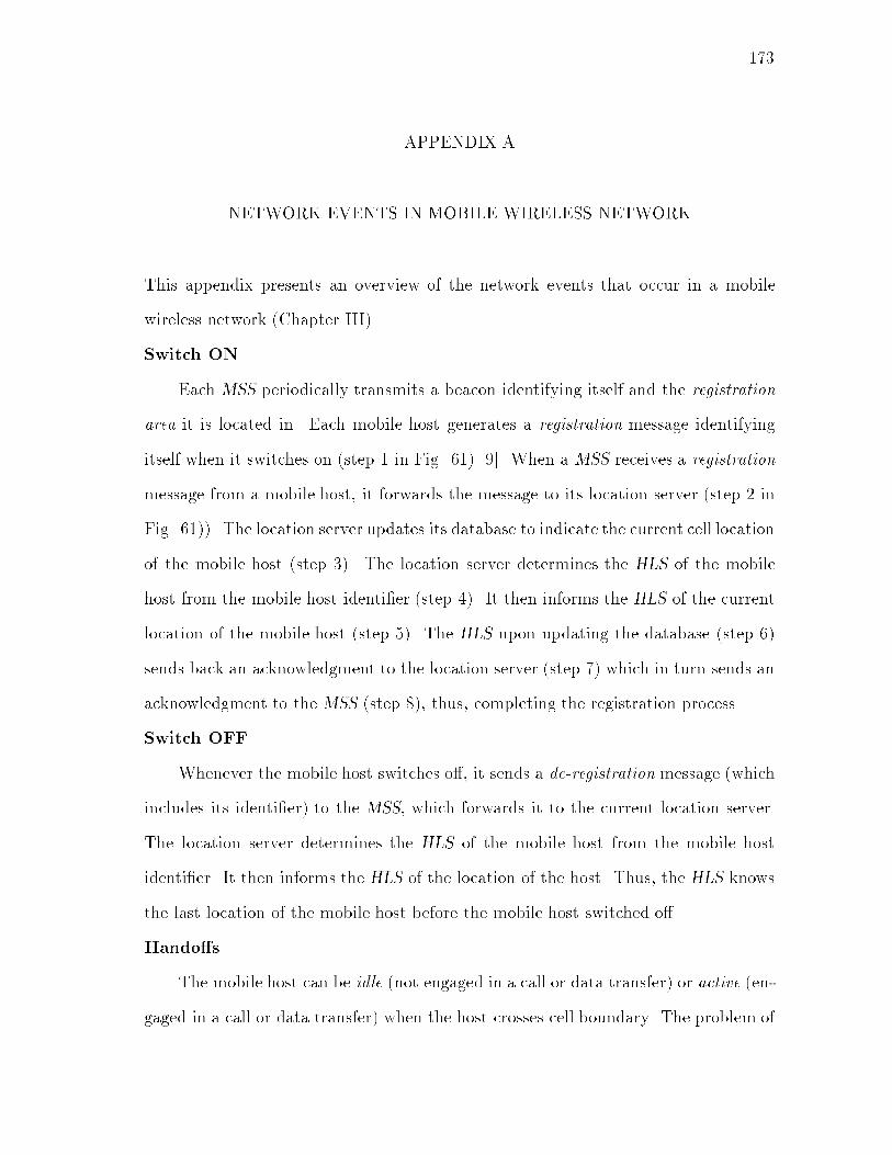
173APPENDIX ANETWORK EVENTS IN MOBILE WIRELESS NETWORKThis appendix presents an overview of the network events that occur in a mobilewireless network (Chapter III).Switch ONEach MSS periodically transmits a beacon identifying itself and the registrationarea it is located in. Each mobile host generates a registration message identifyingitself when it switches on (step 1 in Fig. 61) [9]. When a MSS receives a registrationmessage from a mobile host, it forwards the message to its location server (step 2 inFig. 61)). The location server updates its database to indicate the current cell locationof the mobile host (step 3). The location server determines the HLS of the mobilehost from the mobile host identi�er (step 4). It then informs the HLS of the currentlocation of the mobile host (step 5). The HLS upon updating the database (step 6)sends back an acknowledgment to the location server (step 7) which in turn sends anacknowledgment to the MSS (step 8), thus, completing the registration process.Switch OFFWhenever the mobile host switches o�, it sends a de-registration message (whichincludes its identi�er) to the MSS, which forwards it to the current location server.The location server determines the HLS of the mobile host from the mobile hostidenti�er. It then informs the HLS of the location of the host. Thus, the HLS knowsthe last location of the mobile host before the mobile host switched o�.Hando�sThe mobile host can be idle (not engaged in a call or data transfer) or active (en-gaged in a call or data transfer) when the host crosses cell boundary. The problem of

1741

2

id LS

mh

ls

mss

mh_HLS

mh ls

HLSmh_HLSmh

id

id MSSmh mss

3

4 5

6

7

8Fig. 61. Mobile Host Switches ONactive hando�s are beyond the scope of this work. Apart from location management,active hando�s involve connection management issues, e.g., connectivity, in-order de-livery (in wireless ATM) etc. Here we will describe a procedure for idle hando�s [9].Please refer to Fig. 62 for this discussion. The mobile host mh upon detecting aid

mh

MSS

mss1->mss2

1

ls

mss1 mss2

mh mh

2

3

46

5

Cell 1 Cell 2Fig. 62. Hando�stronger signal from mss2 initiates the hando� procedure by sending a hando�-initmessage to mss2 (step 1 in Fig. 62). This message includes the identi�ers of mh and

175the oldMSS, i.e., mss1. The mss2 upon receiving the hando�-init message requestsmss1 to transfer the host information (user pro�le, etc.) (steps 2 and 3). The mss2then sends an update message to the location server (ls) of its registration area (step4). The ls updates its database and sends back an acknowledgment (steps 5 and 6).The HLS database is not updated during hando�s.

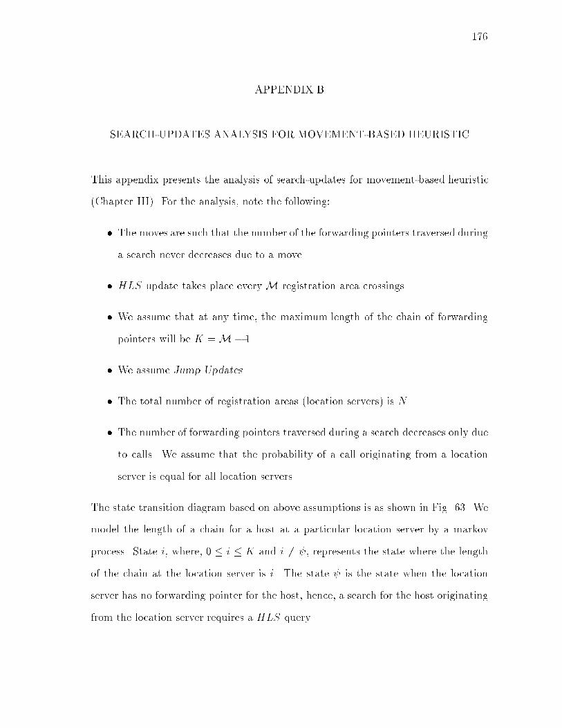
176APPENDIX BSEARCH-UPDATES ANALYSIS FOR MOVEMENT-BASED HEURISTICThis appendix presents the analysis of search-updates for movement-based heuristic(Chapter III). For the analysis, note the following:� The moves are such that the number of the forwarding pointers traversed duringa search never decreases due to a move.� HLS update takes place everyM registration area crossings.� We assume that at any time, the maximum length of the chain of forwardingpointers will be K =M� 1.� We assume Jump Updates.� The total number of registration areas (location servers) is N .� The number of forwarding pointers traversed during a search decreases only dueto calls. We assume that the probability of a call originating from a locationserver is equal for all location servers.The state transition diagram based on above assumptions is as shown in Fig. 63. Wemodel the length of a chain for a host at a particular location server by a markovprocess. State i, where, 0 � i � K and i 6= , represents the state where the lengthof the chain at the location server is i. The state is the state when the locationserver has no forwarding pointer for the host, hence, a search for the host originatingfrom the location server requires a HLS query.

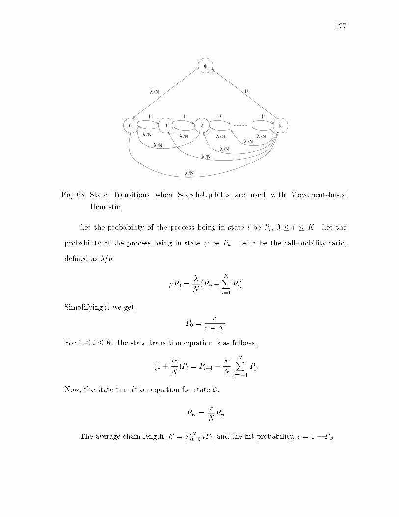
177λ /N

λ /N

λ /N λ /N

λ /N

λ /N

λ /Nλ /N

λ /N

λ /N

0 1

ψ

2 K

µ µ µ µ

µ

Fig. 63. State Transitions when Search-Updates are used with Movement-basedHeuristicLet the probability of the process being in state i be Pi, 0 � i � K. Let theprobability of the process being in state be P . Let r be the call-mobility ratio,de�ned as �=�. �P0 = �N (P + KXi=1 Pi)Simplifying it we get, P0 = rr +NFor 1 � i � K, the state transition equation is as follows;(1 + irN )Pi = Pi�1 + rN KXj=i+1PjNow, the state transition equation for state ,PK = rN P The average chain length, k0 = PKi=0 iPi, and the hit probability, s = 1� P .

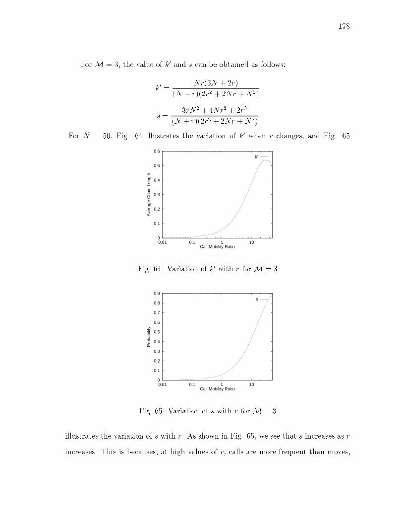
178For M = 3, the value of k0 and s can be obtained as follows:k0 = Nr(3N + 2r)(N + r)(2r2 + 2Nr +N2)s = 3rN2 + 4Nr2 + 2r3(N + r)(2r2 + 2Nr +N2)For N = 50, Fig. 64 illustrates the variation of k0 when r changes, and Fig. 650

0.1

0.2

0.3

0.4

0.5

0.6

0.01 0.1 1 10

Ave

rage

Cha

in L

engt

h

Call Mobility Ratio

k’

Fig. 64. Variation of k0 with r for M = 30

0.1

0.2

0.3

0.4

0.5

0.6

0.7

0.8

0.9

0.01 0.1 1 10

Pro

babi

lity

Call Mobility Ratio

s

Fig. 65. Variation of s with r for M = 3illustrates the variation of s with r. As shown in Fig. 65, we see that s increases as rincreases. This is becauses, at high values of r, calls are more frequent than moves,

179and since we are using jump updates, the probability of the location informationbeing obtained from the location server itself is high.

180APPENDIX CSEARCH-UPDATES ANALYSIS FOR SEARCH-BASED HEURISTICThis appendix presents the analysis of search-updates for search-based heuristic (Chap-ter III). For the analysis, note the following:� The moves are such that the number of the forwarding pointers traversed duringa search never decreases due to a move.� HLS update takes place upon every search, i.e., S = 1.� We assume Jump Updates.� The total number of registration areas (location servers) is N .� The number of forwarding pointers traversed during a search decreases only dueto calls. We assume that the probability of a call originating from a locationserver is equal for all location servers.� The maximum chain length is equal to N, i.e., the number of registration areasin the network. In other words, at least one HLS update is assumed to takeplace before the chain length exceeds N .The state transition diagram based on above assumptions is as shown in Fig. 66. Thestate equations for this state diagram are as follows:P0 = rr +N(1 + r)For i > 0, Pi = 11 + rPi�1

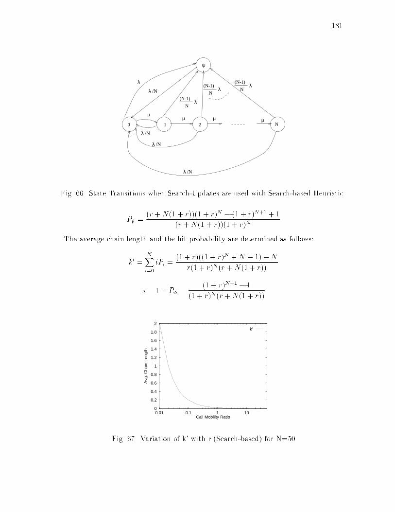
181λ /N

λ /N

λ /N(N-1)

Nλ

(N-1)

Nλ

0 1

ψ

2

µµµµ

λ /N

λ (N-1)

Nλ

NFig. 66. State Transitions when Search-Updates are used with Search-based HeuristicP = (r +N(1 + r))(1 + r)N � (1 + r)N+1 + 1(r +N(1 + r))(1 + r)NThe average chain length and the hit probability are determined as follows:k0 = NXi=0 iPi = (1 + r)((1 + r)N +N + 1) +Nr(1 + r)N (r +N(1 + r))s = 1 � P = (1 + r)N+1 � 1(1 + r)N (r +N(1 + r))0

0.2

0.4

0.6

0.8

1

1.2

1.4

1.6

1.8

2

0.01 0.1 1 10

Avg

. Cha

in L

engt

h

Call Mobility Ratio

k’

Fig. 67. Variation of k' with r (Search-based) for N=50

1820.0196

0.01965

0.0197

0.01975

0.0198

0.01985

0.0199

0.01995

0.02

0.01 0.1 1 10

Pro

babi

lity

Call Mobility Ratio

s

Fig. 68. Variation of s with r (Search-based) for N=50For N = 50, Fig. 67 illustrates the variation of k0 when r changes, and Fig. 68illustrates the variation of s with r. Unlike the movement-based heuristic, the hitprobability for search-based heuristic is very low and also reduces with increasing r.This is because in search-based heuristic an HLS update takes upon every search.The forwarding pointer maintenance policy explained in Section 3 requires that theforwarding pointers be purged during every HLS update. Thus, as r increases, thelifetime of forwarding pointer at a location server reduces, thus the hit probabilityreduces too.

183APPENDIX DPROOF OF CORRECTNESSThis appendix presents an outline of the proof of correctness for the algorithms pre-sented in Chapter V.For the sake of convenience, let us introduce two terms, namely, root node anda�ected node. A root node is a node that initiates the cluster update algorithm,whereas a�ected node is a node whose clusters may be a�ected by the algorithminitiated by the root node. For the various types of events listed in Chapter V, let usdetermine the root node(s) and the a�ected node(s).� Switch ON: The new node is the root node. The neighbors of the new nodeare the a�ected nodes.� Switch OFF: The node n that is determined using the arbitration procedureexplained in Section C.2, is the root node. The neighbors of the node n are thea�ected nodes.� Connection between nodes A and B: The node (A or B) with the largerid is the root node. The common neighbors of A and B are the a�ected nodes.� Disconnection between nodes A and B: The node (say, A) with the largerid is the root node. The neighbors of the root node are the a�ected nodes. Thenode (say, B) other than the root node adds new clusters and does not removeany clusters.Each algorithm comprises of the following basic steps:

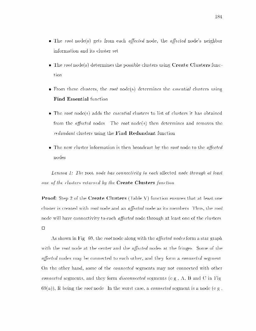
184� The root node(s) gets from each a�ected node, the a�ected node's neighborinformation and its cluster set.� The root node(s) determines the possible clusters using Create Clusters func-tion.� From these clusters, the root node(s) determines the essential clusters usingFind Essential function.� The root node(s) adds the essential clusters to list of clusters it has obtainedfrom the a�ected nodes. The root node(s) then determines and removes theredundant clusters using the Find Redundant function.� The new cluster information is then broadcast by the root node to the a�ectednodes.Lemma 1: The root node has connectivity to each a�ected node through at leastone of the clusters returned by the Create Clusters function.Proof: Step 2 of the Create Clusters (Table V) function ensures that at least onecluster is created with root node and an a�ected node as its members. Thus, the rootnode will have connectivity to each a�ected node through at least one of the clusters.2 As shown in Fig. 69, the root node along with the a�ected nodes form a star graphwith the root node at the center and the a�ected nodes at the fringes. Some of thea�ected nodes may be connected to each other, and they form a connected segment.On the other hand, some of the connected segments may not connected with otherconnected segments, and they form disconnected segments (e.g., A, B and C in Fig.69(a)), R being the root node. In the worst case, a connected segment is a node (e.g.,

185C in Fig. 69(a). In such a case, all a�ected nodes are disconnected from each other.When the root node R switches ON or moves into the vicinity of the nodes in A, B andC, the root node provides connectivity between the disconnected segments through it.It should thus be ensured that the a�ected nodes in the disconnected segments becomecluster-connected after the execution of Find Essential function at the root node (asin Fig. 69(c)). This is because, even if there is a path between these disconnectedsegments through the root node, there may not be any path between them usingclusters. This will violate the cluster-connectivity criteria.Connected Segment

Essential Cluster

(b) New node R

(c) After Find Essential

(a) Disconnected Segments

C

B

R

A

B

C

A A

R C

B

Fig. 69. Clusters formed by Find-EssentialLemma 2: The a�ected nodes in the di�erent disconnected segments becomecluster-connected after the execution of Find Essential function at the root node.Proof: Steps 4-9 of the Find Essential function ensures that there is an essen-tial cluster between at least one node in each connected segment and the root node.Thus, after the execution of Find Essential, there is cluster-connectivity betweenthe a�ected nodes in di�erent disconnected segments. 2

186Lemma 3: Nodes that were cluster-connected before the network event occurred,will remain cluster-connected after the removal of redundant clusters by the root node.Proof: The root node executes the Find Redundant function to determine redun-dant clusters. This function determines redundant clusters based on De�nition 6,which ensures that if a cluster is redundant, removal of the cluster does not a�ect thecluster-connectivity of the graph. 2Theorem 1: Given a cluster-connected graph, the graph remains cluster-connectedafter any network event.Proof: The proof follows from Lemma 1, Lemma 2 and Lemma 3. 2

187APPENDIX ERANDOM GRAPH GENERATORThis appendix presents the algorithm used to generate random graphs (Chapter V).The random graph generator is based on the `labeling' algorithm presented in [27].The input to this graph generator is N and D, where N is the number of nodes in thenetwork, and D is the average degree of the network. We use a `labeling' algorithm togenerate random spanning trees with N nodes. Then we randomly add (ND2 �(N�1))links, so that the average degree in the �nal network is D. The algorithm is presentedin Table XIII.

188Table XIII. Random Graph Generator ProcedureProcedure Random Graph Generator(N ,D);Begin;1. Node list I = [1...N]; Edge list T = ; ;2. Generate a sequence S of (N � 2) random labels in the range [1,N];3. while (jSj > 0)4. Look for the smallest label i1 in I that is not in S;5. T = T [ (i1; s1) ;6. Remove i1 from I and s1 from S ;7. T = T [ (i1; i2) ;8. remaining = ND2 � (N � 1) ;9. while (remaining > 0)10. Randomly generate 2 labels (i,j) s.t., (i; j) =2 T ;11. T = T [ (i; j) ;12. remaining = remaining� 1 ;End;

189VITAP. KrishnaAcademic Degrees:B.S.(Hons.)Department of Electrical EngineeringRegional Engineering College, Rourkela, 1990.M.S.Department of Electrical EngineeringTexas A&M University, 1992Field of Specialization:Computer SciencePermanent mailing address:Apt. 2, 37/B Southern AvenueCalcutta 700029India