On a class of rotating gravitational waves

On a class of rotating gravitational waves

This article has been downloaded from IOPscience. Please scroll down to see the full text article.

2000 Class. Quantum Grav. 17 533

(http://iopscience.iop.org/0264-9381/17/3/302)

Download details:

IP Address: 128.206.162.204

The article was downloaded on 27/09/2010 at 14:57

Please note that terms and conditions apply.

View the table of contents for this issue, or go to the journal homepage for more

Home Search Collections Journals About Contact us My IOPscience

http://iopscience.iop.org/page/terms

http://iopscience.iop.org/0264-9381/17/3

http://iopscience.iop.org/0264-9381

http://iopscience.iop.org/

http://iopscience.iop.org/search

http://iopscience.iop.org/collections

http://iopscience.iop.org/journals

http://iopscience.iop.org/page/aboutioppublishing

http://iopscience.iop.org/contact

http://iopscience.iop.org/myiopscience

Class. Quantum Grav.17 (2000) 533–549. Printed in the UK PII: S0264-9381(00)06000-7

On a class of rotating gravitational waves

Bahram Mashhoon†, James C McClune† and Hernando Quevedo‡† Department of Physics and Astronomy, University of Missouri at Columbia, Columbia,MO 65211, USA‡ Instituto de Ciencias Nucleares, Universidad Nacional Autonoma de Mexico, AP 70-543,04510 Mexico DF, Mexico

Received 14 July 1999, in final form 11 October 1999

Abstract. A class of solutions of the gravitational field equations describing vacuum spacetimesoutside rotating cylindrical sources is presented. The spacetime metric for this class is given byequation (35); to render this metric explicit, one must solve the nonlinear differential equation(31). A subclass of these solutions could correspond to the exterior gravitational fields ofrotating cylindrical systems that emit gravitational radiation. This class has a special solution—corresponding to the exact solution (32) of equation (31)—in common with the Robinson–Trautmangravitational wave spacetimes, namely, the Siklos solution. The properties of rotating gravitationalwaves are briefly investigated. In particular, we discuss the energy density of these waves usingthe gravitational stress–energy tensor.

PACS numbers: 0420, 0430

1. Introduction

Rotating cylindrically symmetric gravitational waves were first discussed in 1990 [1, 2]†. Theinvestigation of these solutions was motivated by Ardavan’s discovery of the speed-of-lightcatastrophe [3] and its implications concerning gravitation [4]. Previous work is generalized inthe present paper and an extended class of rotating gravitational wave spacetimes is analysed.By a rotating wave we mean radiation that propagates outward or inward and at the sametime has non-trivial azimuthal motion. We find that the solution investigated previously [1, 2]is special, since it is the only member of the extended class studied here that represents thepropagation offreerotating gravitational waves; moreover, we show that this special solutionis locally equivalent to a Robinson–Trautman solution studied by Kerr and Debney and lateron by Siklos.

The gravitational fields under consideration here are given by Ricci-flat spacetimes thatare characterized by a metric of the form

−ds2 = e2γ−2ψ(−dt2 + dρ2) +µ2e−2ψ(ω dt + dφ)2 + e2ψ dz2, (1)

in cylindrical coordinates(ρ, φ, z). Hereγ, µ,ψ andωare functions oft andρ only; moreover,the signature of the spacetime metric is +2 throughout this paper and the speed of light invacuum is set equal to unity. The gravitational field equations for the metric form (1) are given

† There is an error on p 289 of [2] in the discussion of the exterior field of a rotating cylinder. Contrary to the statementin the paper, the exterior vacuum field is not always static. It is, in fact, stationary for high angular momentum. Thishas been shown by Bonnor W B 1980J. Phys. A: Math. Gen.13 2121. BM is grateful to Professor Bonnor forclarifying remarks. Moreover, a typographical error occurs in equation (9):µ,uv should be replaced byµ,vv .

0264-9381/00/030533+17$30.00 © 2000 IOP Publishing Ltd 533

534 B Mashhoon et al

in appendix A. The physical motivations as well as a detailed discussion of certain aspectsof the field equations for metric (1) are contained in previous papers [1, 2], which shouldbe consulted for further background information. Briefly, ansatz (1) is obtained from thegeneral metric of rotating cylindrical gravitational waves with a constant linear polarizationstate by placing a certain restriction on the metric coefficients in order to reduce the numberof unknown functions to four [2]. The spacetime represented by equation (1) admits twocommuting spacelike Killing vectors∂z and∂φ . Though∂z is hypersurface-orthogonal,∂φ isnot; moreover, the isometry group is not orthogonally transitive. Vacuum solutions with twocommuting Killing vector fields without the assumption of orthogonal transitivity have beenconsidered by Gaffet [5]; however, it turns out that Gaffet’s formalism is notdirectlyapplicableto our metric (1), since it is not of the form (1.6) of [5]. To retain our physical conceptions inthis case [1, 2], we prefer to work with the metric in the form (1).

Instead of the variablest andρ, it is convenient to express the gravitational field equationsin terms of the retarded and advanced timesu = t − ρ andv = t + ρ, respectively. Thegravitational potentials for rotating waves are given by

(µψv)u + (µψu)v = 0, (2)

µuv − 18l

2µ−3e2γ = 0, (3)

ωv − ωu = lµ−3e2γ , (4)

γu = 1

2µu(µuu + 2µψ2

u), (5)

γv = 1

2µv(µvv + 2µψ2

v ), (6)

whereψu = ∂ψ/∂u, etc. Here,l is a constant length characteristic of the rotation of thesystem. We assume thatl > 0 throughout this paper that is specifically devoted torotatinggravitational waves. In fact, forl = 0 the waves are non-rotating but expressed in a rotatingframe of reference, since equation (4) implies thatω = ω(t) in this case (cf appendix A).The explicit connection betweenl and the rotation of the waves has been determined via aperturbative treatment in a previous work [2]. Using equation (3), it is possible to eliminateγ

from equations (5) and (6); then, we obtain the following equations:

2µ2ψ2u = 3µ2

u − µµuu +µµuµuuv(µuv)−1, (7)

2µ2ψ2v = 3µ2

v − µµvv +µµvµuvv(µuv)−1. (8)

The integrability condition for this system, i.e.ψuv = ψvu, results in a nonlinear fourth-orderpartial differential equation forµ. Alternatively, one could obtain the same equation forµ bycombining equations (2), (7) and (8), which shows the consistency of the field equations (2)–(6). It is important to notice thatµ cannot be a function ofu or v alone, since this possibilitywould be inconsistent with equation (3). The partial differential equation of fourth order forµ is, however, identically satisfied ifµ is a separable function, i.e.µ = α(u)β(v); this leads,in fact, to the rotating waves discussed earlier [1, 2]. Here we wish to study a more generalsolution of the field equations.

In section 2, we discuss the solution of the field equations (2)–(6) forl 6= 0. We findthat there are two possible classes of solutions. The first class corresponds to known solutionssuch as the stationary exterior field of a rotating cylindrical source, while the second classappears to represent a mixed situation involving rotating gravitational waves. In fact, asubclass of the latter solutions describes the exterior fields of certain rotating sources thatemit gravitational radiation; these solutions approach the special rotating wave solution [1, 2]

On a class of rotating gravitational waves 535

far from their sources. Indeed, the only solution of the second class corresponding to apure gravitational wave spacetime is the special solution [1, 2] that is a Robinson–Trautmansolution (cf appendix B) and is further discussed in section 3. In section 4, some aspects ofthe energy, momentum and pressure of the rotating gravitational waves are discussed usingthe Bel–Robinson tensor [6]. Section 5 contains concluding remarks. The appendices containsome of the detailed calculations.

2. Solution of the field equations

To solve the field equations (2)–(6), let us introduce the functionsU,V andW by

U = µuγu − 12µuu, V = µvγv − 1

2µvv, W = µγuv + 32µuv, (9)

and rewrite equations (5) and (6) as

µψu = ε(µU)1/2, µψv = ε(µV )1/2, (10)

where the symbolsε andε represent either +1 or−1 (i.e.ε2 = ε2 = 1). Using equation (3),it is straightforward to show that

µUv = µuW, µVu = µvW. (11)

Let us now combine relations (10) and (11) in order to satisfy equation (2); the result is

εU−1/2(µvU +µuW) + εV −1/2(µuV +µvW) = 0. (12)

This equation can be written as

U(µuV +µvW)2 = V (µvU +µuW)

2, (13)

which holds if eitherW 2 = UV orµ2uV = µ2

vU ; that is, equation (13) can be factorized intoa fourth- and third-order equation, respectively.

Let us first consider the fourth-order equationW 2 = UV . It follows from this relation andequation (10) thatW = ∓µψuψv. The relationW = −µψuψv is discussed in appendix A;indeed, it is a redundant field equation. In view of this fact, the other possibilityW = µψuψvsimply impliesψuψv = 0; alternatively, this expression forW along withU = µψ2

u andV = µψ2

v can be inserted into equation (11) to obtain relations that when combined withequation (2) in the form 2µψuv = −(µuψv + µvψu) imply ψuψv = 0. If ψ is a functionof eitheru or v alone, then equation (2) implies thatψ must be a constant. The spacetimerepresented by a constantψ turns out to be a common special case of the solutions discussedin this section and isflat. Let us briefly digress here to discuss a subtle point regarding ourapproach. In this paper we attempt to derive the general solution of the field equationsasrevealed by our method. In this way we hope to find thegeneralsolution of the field equations,but there is no guarantee. In fact, the redundancy noted above may indicate a shortcoming ofour approach in this respect. The resolution of this difficulty is beyond the scope of this paper.

Let us next considerµ2uV = µ2

vU . It follows from equation (3) that

γu = 3

2

µu

µ+

1

2

µuvu

µuv, γv = 3

2

µv

µ+

1

2

µuvv

µuv, (14)

which together with equations (9) imply thatµ2uV = µ2

vU is essentially equivalent toµuvv

µv− µvvµuv

µ2v

= µuvu

µu− µuuµuv

µ2u

. (15)

Equation (15) can be written as(lnµv)uv = (lnµu)vu. Letf (u) andg(v) be arbitrary functionsof their arguments and consider the transformation(u, v)→ (x, y) such that

x = f (u) + g(v), y = f (u)− g(v), (16)


fu 6= 0, andgv 6= 0; then, the general solution forµ is thatµ = µ(x), i.e.µ should not dependony.

Let us now proceed to the calculation ofψ . To this end, let us consider a functionL(x)given by

L2(x) = 1

2

(3µ′2 − µµ′′ +µµ

′µ′′′

µ′′

), (17)

where a prime indicates differentiation with respect tox. Equations (7) and (8) can now bewritten as

µ2ψ2u = f 2

uL2, µ2ψ2v = g2

vL2. (18)

Furthermore,

ψu =(∂ψ

∂x+∂ψ

∂y

)fu, ψv =

(∂ψ

∂x− ∂ψ∂y

)gv. (19)

Combining equations (18) and (19), we find that eitherψ is purely a function ofx given byµ2(dψ/dx)2 = L2(x) or ψ is purely a function ofy given byµ2(dψ/dy)2 = L2(x). Thesecases will now be discussed in turn.

2.1. Case (i):ψ = ψ(x)It follows from equation (2) that in this case

dψ

dx= C

µ(x), (20)

whereC is an integration constant. Thusµ(x) is determined byL2(x) = C2. To solve thisdifferential equation, letX = µ′ and note that

L2 = 1

2X2

(µ2 dX

dµ

)−1 d

dµ

(µ3 dX

dµ

). (21)

Moreover, letS = µdX/dµ; then,L2(x) = C2 can be written as

dS

dX= 2

(C2

X2− 1

), (22)

which can be integrated to giveS = −2(D +X + C2/X). HereD is an integration constant.It follows from this result thatµ(x) can be found implicitly from dµ = X(µ) dx, where

µ2 = exp

(−∫

X dX

X2 +DX +C2

). (23)

The spacetime metric in this case can be written in a form that depends only onx. Thatis, it is possible to show—by a transformation of the metric to normal form—that the generalsolution in case (i) has an extra timelike or spacelike Killing vector field∂y . To this end, let usconsider the coordinate transformation(t, ρ, φ, z)→ (T , R,8,Z), wheref (u) = (T +R)/2,g(v) = (−T +R)/2,φ = 8+H(T,R)andz = Z. In this transformationH(T,R) is a solutionof the partial differential equation

−(F +G)∂H

∂T+ (F −G)∂H

∂R+

2

l(F +G)

dµ

dR= 0, (24)

whereF = f −1u , G = g−1

v , R = x andT = y. To prove our assertion, we will show thatunder this coordinate transformation the spacetime metric in case (i) takes the form

−ds2 = P(R)(−dT 2 + dR2) +µ2(R) e−2ψ(R)[�(R) dT + d8]2 + e2ψ(R)dZ2, (25)


which is clearly invariant under a translation inT thus implying the existence of a Killingvector field∂T . It follows from a comparison of the metric forms (1) and (25) that

P(R) = − 2

l2µ3 d2µ

dR2e−2ψ(R), (26)

∂H

∂T= − 1

4ω(F −G) +�(R), (27)

∂H

∂R= − 1

4ω(F +G). (28)

Equations (27) and (28) can be used in equation (24) to show that�(R) = 2l−1 dµ/dR. Itremains to show that the integrability condition for equations (27) and (28), i.e.∂2H/∂R∂T =∂2H/∂T ∂R, is satisfied. It turns out that this relation is indeed true, since it is equivalent tothe field equation (4) forω.

Let us note that the solution of equation (22) implies that in case (i)

d2µ

dR2= − 2

µ

[(dµ

dR

)2

+Ddµ

dR+C2

], (29)

and one can show explicitly that the metric form (25) is flat onceC = 0. ForC 6= 0, the generalsolution of case (i) is not flat. IfP(R) > 0, a simple redefinition of the radial coordinate can beused to cast equation (25) in Lewis form, i.e. solution (25) is a member of the class of exteriorstationary solutions found by Lewis (see [7], ch 20). ForP(R) < 0, the solution containsthree commuting spacelike Killing vectors and belongs to the family of Kasner solutions (see[7], ch 11).

2.2. Case (ii):ψ = ψ(y)It follows from (dψ/dy)2 = L2(x)/µ2 thatψ must be a linear function ofy, since the left-handside of this equation is purely a function ofy, while the right-hand side is purely a functionof x; therefore, each side must be constant. Thusψ = ay + b, wherea andb are constants,andL2 = a2µ2. It turns out that equation (3) is identically satisfied in this case. Usingequation (21), the differential equation forµ can be expressed in terms ofX = µ′ as

X2 d

dµ

(µ3 dX

dµ

)= 2a2µ4 dX

dµ. (30)

If a = 0, ψ is constant and we recover the same flat spacetime solution as in case (i) withC = 0. Therefore, leta 6= 0 and consider a new ‘radial’ coordinater given byr = (a2µ2)−1;then,

r2X2 d2X

dr2+

dX

dr= 0. (31)

The solutionX = constant is unacceptable, since it implies thatγ = −∞. However, there isanother exact solution that is given by

X = ±( 32r)−1/2

, (32)

which turns out to correspond to the special rotating gravitational waves [1, 2] that are thesubject of the next section. It is possible to transform equation (31) to an autonomous form;to this end, let us defineδ and ξ such thatδ = 2/(3rX2) and ξ = −4Xr/(3X3), whereXr = dX/dr. It can then be shown that equation (31) is equivalent to

dξ

dδ= 3

2

ξ(ξ − δ2)

δ(ξ − δ) , (33)


Figure 1. The plot ofξ versusδ for equation (33) illustrating the spiral structure near the singularpoint (1, 1) corresponding to the special solution (32). In fact, the plot displays some of thecharacteristic curves of the autonomous system dδ/dθ = 2δ(ξ − δ) and dξ/dθ = 3ξ(ξ − δ2). Theδ andξ nullclines are represented by broken curvesδ = ξ andξ = δ2, respectively. The criticalpoint(0, 0) is a degenerate singularity of the system, while the other critical point(1, 1) is a simplesingularity.

where(δ, ξ) = (1, 1) represents the special solution (32). This special solution is an isolatedsingularity of the nonlinear autonomous system (33) and the behaviour of characteristics nearthis point indicates that(1, 1) is a spiral point as shown in figure 1.

Let us note here certain general features ofX(r), which is the solution of equation (31).If X(r) is a solution, then so is−X(r). Moreover, equation (31) can be written as(X2

r )r = −2X2r /(r

2X2), which indicates that forX 6= constant the absolute magnitude ofthe slope ofX(r) decreases monotonically asr increases. IfX(r) has a zero atr0 6= 0, thenthe behaviour ofX(r) nearr0 is given by

X(r) = ±√

2

r0

(r

r0− 1

)1/2[1 +

1

2

(r

r0− 1

)− 3

76

(r

r0− 1

)2

+ · · ·], (34)

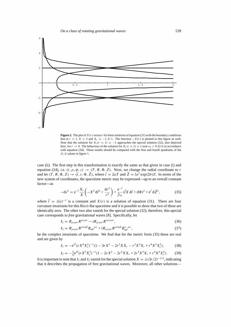
for r > r0. These results are illustrated in figure 2.Once a solutionX(r) of equation (31) is given, one can find a solution of the field

equations in case (ii). It turns out that in general such a solution is not a pure gravitationalwave. The only exception is the special solution (32). To demonstrate this, let us firstconsider a transformation of the spacetime metric (1) to the normal form appropriate for


Figure 2. The plot ofX(r) versusr for three solutions of equation (31) with the boundary conditionsthat atr = 1, X = 2 andXr = −1, 0, 1. The function−X(r) is plotted in this figure as well.Note that the solution forXr(r = 1) = −1 approaches the special solution (32), also depictedhere, forr → 0. The behaviour of the solution forXr(r = 1) = 1 nearr0 ' 0.22 is in accordancewith equation (34). These results should be compared with the first and fourth quadrants of the(δ, ξ)-plane in figure 1.

case (ii). The first step in this transformation is exactly the same as that given in case (i) andequation (24), i.e.(t, ρ, φ, z) → (T , R,8,Z). Next, we change the radial coordinate torand let(T , R,8,Z)→ (t , r,8, Z), wheret = 2aT andZ = la2 exp(2b)Z. In terms of thenew system of coordinates, the spacetime metric may be expressed—up to an overall constantfactor—as

−ds2 = e−tXr

X

(−X2 dt2 +

dr2

r3

)+

e−t

l2r(lX dt + d8)2 + et dZ2, (35)

where l = (la)−1 is a constant andX(r) is a solution of equation (31). There are fourcurvature invariants for this Ricci-flat spacetime and it is possible to show that two of these areidentically zero. The other two also vanish for the special solution (32); therefore, this specialcase corresponds tofreegravitational waves [8]. Specifically, let

I1 = RµνρσRµνρσ − iRµνρσR∗µνρσ , (36)

I2 = RµνρσRρσαβRαβµν + iRµνρσRρσαβR∗αβ

µν, (37)

be the complex invariants of spacetime. We find that for the metric form (35) these are realand are given by

I1 = −e2t (rX4X2r )−1(1− 3rX2 − 2r2XXr − r3X3Xr + r4X2X2

r ), (38)

I2 = − 34e3t (rX5X3

r )−1(1− 2rX2 − 2r2XXr + 2r3X3Xr + r4X2X2

r ). (39)

It is important to note thatI1 andI2 vanish for the special solutionX = ±(3r/2)−1/2, indicatingthat it describes the propagation of free gravitational waves. Moreover, all other solutions—


which do not describefreegravitational waves—are singular fort →∞, sinceI1 andI2 bothdiverge in the infinite ‘future’. Thus all such solutions ‘evolve’ to states that are ultimatelysingular. The singular nature of the special solution (32) has been discussed previously [1, 2].It is important to point out that for some solutionsX(r) of equation (31),r is in fact thetemporal coordinate in the spacetime metric (35). One can show thatt satisfies the scalar waveequation,gµν9;µν = 0, in the spacetime given by the metric form (35); therefore,t must ingeneral be interpreted as the scalar potential for the cylindrical gravitational waves. Indeed,exp(t/2) is the scalar magnitude of the spacelike Killing vector associated with translationalinvariance along the axis of cylindrical symmetry.

It is clear from equation (31) and figure 2 that asr → 0, X(r) → ±(3r/2)−1/2 for asubclass of the spacetimes under consideration here; indeed, it is simple to check thatI1→ 0andI2 → 0 asr → 0 for the solution given in figure 2 withXr(r = 1) = −1. Moreover,I1 and I2 diverge asr → ∞. In fact, inspection of the first quadrant of figure 1 showsthat these properties are shared by many solutions withXr/X < 0. We might expect thatsuch solutions correspond to the exterior field of a rotating and radiating cylindrical sourcesuch that very far from the symmetry axis the metric would nearly describe free rotatinggravitational waves given by the unique special solution (32); of course, one would need tofind an appropriate interior solution for the source. In this case, it is useful to introduce a newradial coordinateR = r−1/2 exp(−t/2), which is the magnitude of the Killing vector∂8 upto a proportionality constant. Thusr → 0 or t → −∞ corresponds toR → ∞, so that faraway from the symmetry axisI1 → 0 andI2 → 0, while for r → ∞ or t → ∞, R → 0andI1 andI2 are both divergent. It follows that the axis of cylindrical symmetry is alwayssingular and that far from the axis the spacetime approaches the special free rotating wavesolution that has singularities and is discussed in the next section. For a singular axis, thedefinition of axisymmetry is problematic [9]; hence, difficulties may arise in interpreting thesesolutions as rotatingcylindrical gravitational waves. Such radiation is presumably emitted bya regular rotating cylindrical source; the waves then propagate outward to become essentiallyfree rotating waves far from the source. A detailed interpretation as well as the matching ofthe exterior solution with an interior solution is beyond the scope of this work.

The general rotating wave solution (35) turns out to be of type I in the Petrov classification.Thus rotating gravitational wave spacetimes are algebraically general except in the case of thespecial solution (32), which is algebraically special and of Petrov type III. This solution turnsout to be locally equivalent to a special Robinson–Trautman solution as shown in appendix B.The Robinson–Trautman class of gravitational wave spacetimes only involves algebraicallyspecial solutions and is therefore distinct from the class of rotating wave spacetimes presented inthis paper. It is interesting to note that the Robinson–Trautman class can be simply generalizedby the inclusion of a cosmological constant3 (see [7], ch 24). Thus the special rotating wavesolution has a3 6= 0 generalization studied by Siklos (see equation (11.45) on p 134 of [7]).Further investigation is needed to determine whether the class of rotating gravitational wavescan be generalized to include a cosmological constant.

The class of rotating gravitational waves is given by the metric form (35), whereX(r) isa solution of the nonlinear differential equation (31). This equation remains invariant underthe scale transformationσ : (r,X) → (σ 2r, σ−1X), whereσ is a constant. The spacetime(35) involving asolutionof (31) that also remainsinvariant under such scaling—such as thespecial solution (32)—would then contain a third Killing vector. In fact, inspection of themetric form (35) reveals that it remains unchanged to first order inε0, 0< ε0 � 1, under thetransformationst → t − 2ε0, r → (1 + ε0)r, X → (1− ε0/2)X, 8 → (1− ε0/2)8 andZ → (1 + ε0)Z. This observation indicates the existence of a third Killing vector given byKµ = (−2, r,−8/2, Z); moreover,Kµ is not hypersurface-orthogonal. The existence of this


additional spacelike Killing vector for the special solution (32) does not extend to the generalsolution. The quantitiesδ andξ in equation (33) are invariant under the scale transformationσ ; however, a general solutionX(r) of equation (31) isnot. To our knowledge, only thespecial solution contains a three-parameter group of isometries. It is shown in appendix B thatthis solution is of type VIh, with h = − 1

9, in the Bianchi classification and that it is locallythe same as a special Robinson–Trautman solution. Thus the rotating vacuum solutions ofthe gravitational field equations for the metric form (1) in cases (i) and (ii) either contain anadditional Killing vector field, in which case they are known [7], or they are given by themetric form (35), whereX(r) 6= ±(3r/2)−1/2 must apparently be obtained numerically fromequation (31). A completenumericalinvestigation of possible solutions given by equations (31)and (35) and partly revealed in figure 2 is beyond the scope of this paper. However, it is possibleto work out some aspects of the energy density and pressure of the rotating gravitational waves.This subject is taken up in section 4.

Finally, let us note that the unique special solution corresponding to free gravitationalwaves (32) can be written in terms ofµ andx as dµ/dx = ±( 2

3)1/2aµ, which can be easily

solved to show thatµ depends exponentially uponx = f (u) + g(v). This means simply thatµ can be written asµ = α(u)β(v), whereα andβ are arbitrary functions. The next section isdevoted to a discussion of the properties of this solution beyond what is already known fromprevious studies [1, 2].

3. Free rotating gravitational waves

Free non-rotating cylindrical gravitational wave solutions of Einstein’s equations were firstdiscussed by Beck [10]. These solutions have been the subject of many subsequentinvestigations [8, 11, 12]. The solutions considered in this section can be interpreted in termsof simple cylindrical waves that rotate [2], though they are all locally equivalent to a specialRobinson–Trautman solution that has been investigated by Kerr and Debney and Siklos (cfappendix B).

The special solution (32) for free rotating gravitational waves is given by

µ = α(u)β(v), ψ =√

32 ln

α

β, (40)

γ = 1

2ln

[8

l2(αβ)3αuβv

], ωv − ωu = 8

lαuβv. (41)

It turns out that in this case equation (2) is equivalent to the scalar wave equation forψ in thebackground geometry given by equation (1); therefore, the functionψ , which is a mixture ofingoing and outgoing waves according to equation (40), has the interpretation of the scalarpotential for the free rotating gravitational waves. The solution (40) and (41) cannot be thoughtof as a collision between outgoing and ingoing gravitational waves, since the field equationsdo not admit solutions for whichµ = µ(u) orµ = µ(v). That is, there is no purely outgoingsolution just as there is no purely ingoing solution. The curvature invariants all vanish for thespecial solution (32); in fact, the free waves are of type III in the Petrov classification [1].

The spacetime given by equations (40) and (41) is singular. In fact, the analysis of thespacetime curvature indicates that moving singular cylinders appear wheneverα, β, αu or βvvanishes. It is interesting to consider the nature of the symmetry axis for rotating waves, sincein these solutions the axis does not, in general, satisfy the condition of elementary flatness. Iffor an infinitesimal spacelike circle around the axis of symmetry the ratio of circumference toradius goes to 2π as the radius goes to zero, the condition of elementary flatness is satisfiedfor the axis under consideration. In our case, this means thatµ2/(e2γ ρ2) → 1 asρ → 0.


For simple cylindrical waves (i.e. Beck’s solution) we haveµ = ρ and hence the condition ofelementary flatness is thatγ → 0 asρ → 0. In general, Beck’s fields can be divided into twoclasses: the Einstein–Rosen waves [11] and the Bonnor–Weber–Wheeler waves [12]. In theformer class, the axis does not satisfy the condition of elementary flatness; in fact, the axis isnot regular either. It is a singularity of spacetime and is therefore interpreted as the source ofthe cylindrical waves which are otherwise free of singularities. In the latter case, the axis doessatisfy the condition of elementary flatness and is, moreover, regular. The waves presumablyoriginate at infinity: incoming waves implode on the axis and then move out to infinity withno singularities in the finite regions of spacetime. It is therefore clear thatnocaustic cylindersappear regardless of the nature of the axis. They do appear, however, when the wavesrotate.We are therefore led to regard the appearance of moving singular cylinders in our solution asbeing due to the rotation of the waves. It is important to emphasize the absence of a directcausal connection between the violation of elementary flatness at the axis and the presenceof singular cylinders: the axis is static while the singularity is in motion, and the conditionof elementary flatness involves the gravitational potentials (gµν), while the singularity of thefield has to do with the spacetime curvature. In fact, it is possible to find instances of exactsolutions for which the axis is elementary flat but singular [13]. A discussion of related issuesis contained in [9].

In spacetime regions between the extrema ofα andβ, the solution (40) and (41) can bereduced to a normal form in whichα andβ are linear functions of their arguments [1]. Withfurther elementary coordinate transformations, the normal form can be reduced to two specialsolutions which are of interest: (a)α = σ0u, β = σ0v and (b)α = σ0u, β = −σ0v. Hereσ0 = ±(l0)−1/2, wherel0 is a constant length whose introduction is necessary on dimensionalgrounds. The metrics for these cases are, respectively,

−ds2 = 8(uv)3

l40l2

(u

v

)−√6

(−dt2 + dρ2) +(uv)2

l20

(u

v

)−√6(8ρ

l0ldt + dφ

)2

+

(u

v

)√6

dz2

and

−ds2 = 8(uv)3

l40l2

(−uv

)−√6

(−dt2 + dρ2) +(uv)2

l20

(−uv

)−√6(8ρ

l0ldt − dφ

)2

+

(−uv

)√6

dz2.

To ensure that the spacetime metric is real, case (a) must be limited to(u > 0, v > 0) or(u < 0, v < 0). Similarly, case (b) must be limited to(u > 0, v < 0) or (u < 0, v > 0). Ineither case the hypersurfacesu = 0 andv = 0 are curvature singularities. Since the laws ofphysics break down very close to these surfaces, it appears that the consideration of boundaryconditions across such surfaces would be without physical significance. In case (b),ρ is atemporal coordinate andt is a spatial coordinate. The transformation(t → ρ, ρ → t), orequivalently(u → −u, v → v), brings the metric to a form which reduces to case (a) witha further coordinate transformationφ → φ + 8tρ/(l0l). Therefore, only the normal form incase (a) will be considered in the remainder of this paper.

The geodesic equation for free rotating gravitational wave spacetimes is discussed inappendix C.

4. The gravitational stress–energy tensor

In our recent work [6], a fundamental pseudo-local gravitoelectromagnetic stress–energytensor has been defined via a certain averaging procedure in a Fermi frame along the pathof a geodesic observer. The result can then be pointwise extended to arbitrary observers,following the standard manner involving instantaneous measurements, in accordance with


the basic assumption of locality in general relativity. For Ricci-flat spacetimes, thegravitoelectromagnetic stress–energy tensor becomes the gravitational stress–energy tensorTµν given by

Tµν = L2

12πG0Tµνρσ λ

ρ

(0)λσ(0) =

L2

12πG0Tµν(0)(0), (42)

whereG0 is Newton’s constant,L is a constant length-scale characteristic of the field underconsideration,Tµνρσ is the Bel–Robinson tensor [6, 8, 14] defined by

Tµνρσ = 12(RµξρζRν

ξσζ +RµξσζRν

ξρζ )− 1

16gµνgρσRαβγ δRαβγ δ, (43)

andλµ(0) = dxµ/dτ is the vector tangent to the timelike path of the observer. The gravitationalstress–energy tensor is expected to provideapproximatemeasures of the average gravitationalenergy, momentum and stress in the neighbourhood of the observer.

The result of the calculation ofTµν for a simple class of linearly polarized planegravitational waves is given in our 1997 paper [6]. A systematic study ofTµν for gravitationalradiation spacetimes (such as, for example, Beck’s fields) would be a worthwhile endeavour.Here, however, we focus attention on rotating waves and present the results of certain relativelytractable calculations.

Let us imagine a spacetime given by the metric form (35), whereX(r) is a solution ofequation (31) such that far from the symmetry axis it approaches the free rotating gravitationalwaves. As is evident from figure 2, for such solutions of equation (31),XXr < 0. Inspection ofthe metric form (35) then reveals that in this caset is a spatial coordinate andr is the temporalcoordinate. Consider now the class of static observers whose orthonormal tetrad frame, in(t , r,8, Z) coordinates, consists of the temporal axis(

−e−tXr

r3X

)−1/2

(0, 1, 0, 0) (44)

as well as the spacelike unit vector exp(−t/2) (0, 0, 0, 1) parallel to the axis of symmetry.The other two spatial axes will be ignored for the sake of simplicity. It can be shown that theenergy density of the gravitational field according to the static observers is

ρg =(

L2

96πG0

)e2t

X2X2r

[1 +

1

2rX2(1− r2XXr)(1 + rX2 − r2XXr)

], (45)

while the flux of gravitational energy parallel to the axis of symmetry vanishes. However, theradiation has pressure along this direction given by

pg =(

L2

96πG0

)e2t

X2X2r

. (46)

The gravitational energy density and pressure are positive andpg < ρg. For the special exactsolution (32) corresponding to free rotating waves, these results reduce toρg = 3pg andpg = (3L2/32πG0)r

4 exp(2t ); indeed, the partial equation of statepg = ρg/3 appears to beconsistent with the interpretation of this solution in terms offreegravitational waves.

It would be interesting to study the energy of rotating gravitational waves along theworldline of a geodesic observer. However, the spacetime metric for the rotating waves (35) isgiven explicitly only for the case of the exact solution (32) of the differential equation (31). Thisunique solution is approached asymptotically by the rotating-wave solutions very far from thesymmetry axis. For the sake of simplicity, we therefore restrict attention to the special solution(32) that, according to the results presented in section 3, corresponds to thefreerotating waves.


Figure 3. The functionsρ(τ)/ l0 andφ(τ) given by equations (47) and (48), respectively, withφ0 = π/2 are plotted here as polar coordinates (i.e. abscissa= ρ cosφ and ordinate= ρ sinφ).This represents the trajectory of a particle following the ‘radial’ geodesic given by equations (47)and (48). The particle starts atτ = 0 fromρ = 0 and moves counterclockwise until it returns to asingular axis(ρ = 0) at τ = l0. The return trip takes only about 10% of the total proper timel0.

To determine the energy density of this radiation field measured by a geodesic observer,it is first necessary to consider a solution of the geodesic equation discussed in appendix C.Let us therefore choose a ‘radial’ geodesic of the free rotating waves given by

t = 12 l0(ζ

1/p + ζ 1/q), ρ = − 12 l0(ζ

1/p − ζ 1/q), (47)

φ = 12

√5(ζ 2/p − ζ 2/q −

√32 ζ

4/5)

+ φ0, z = z0, (48)

where we have used equations (C7) and (C8) of appendix C together with the metric in normalform given in section 3, i.e.α(u) = u/l1/20 andβ(v) = v/l1/20 , and we have fixed the constantsin these equations such thatτ1 = τ2 = l0, 2c1 = l1−p/20 and 2c2 = l1−q/20 . Note that the scalingparameterl0 is therefore related to the intrinsic rotation parameterl via 2l0 =

√5 l; moreover,

φ0 andz0 are constants,p = 4− √6, q = 4 +√

6 andζ is defined byζ = 1− τ/ l0. Theobserver under consideration here starts at the symmetry axisρ = 0, which is regular atτ = 0,and returns to it atτ = l0 when it is singular. The trajectory of this observerρ(φ) is depictedin figure 3.

Imagine now an orthonormal tetrad frameλµ(α) that is parallel propagated along this timelikeworldline. It is simple to work out explicitly two axes of the tetrad: the time axis and the spatialaxis parallel to the symmetry axis. These are given byλ

µ

(0) = dxµ/dτ using equations (47)and (48) andλµ(3) = ζ−3/5δ

µ

3 , respectively. It follows from the projection ofTµνρσ on theseaxes that along the geodesic the gravitational radiation energy density is given by

T(0)(0) = 36

625πG0

L2

(l0 − τ)4 , (49)

while the energy flux along the symmetry axis vanishes,T(0)(3) = 0, as expected. There is,


however, radiation pressure along thez-axis, which is given by

T(3)(3) = 3

125πG0

L2

(l0 − τ)4 . (50)

The energy density and the pressure measured by the geodesic observer both diverge at thesingularity τ = l0. Note thatT(3)(3)/T(0)(0) = 5

12, which is less than unity as would beexpected for the ratio of pressure to density. The characteristic length-scale associated withrotating gravitational waves isl; therefore, the constant lengthL could be chosen to be simplyproportional tol = 2l0/

√5.

5. Conclusion

A discussion of the rotating waves is provided starting from a certain ansatz (1) for the spacetimemetric. A new class of such spacetimes is found that is given by equations (35) and (31).To make the spacetime metric explicit, a solution of the nonlinear differential equation (31)is required. To find such solutions in general, one must resort to numerical investigations;however, a detailed numerical study of rotating wave spacetimes is beyond the scope of thiswork. The differential equation (31) has a special exact solution that corresponds to freerotating gravitational waves studied in two previous papers [1, 2]; this solution is shown to belocally equivalent to the Siklos solution, which is a special Robinson–Trautman solution.

We present a brief discussion of the properties of the general solution as well as a furthertreatment of the special solution with particular emphasis on the stress–energy content of therotating waves. Expressions are provided for the gravitational energy density and the pressureof the radiation parallel to the axis of cylindrical symmetry that are in agreement with physicalexpectations.

Acknowledgments

We would like to thank an anonymous referee of a previous version of this paper for pointingout the existence of the additional Killing vector of the solution corresponding to equation (32).This work has been supported by CONACYT, Mexico, grant no 3567–E and DGAPA-UNAM,grant no 121298.

Appendix A. Field equations

The gravitational field equations for the vacuum region under consideration in this paper areRµν = 0. Using the spacetime metric (1) we find

Rtt = 1

µ(E1 +E2)− µω2e−2γ (E1− E2)− ω

µE4 − 1

µE7,

Rtρ = − ω

2µE3− 1

µE6,

Rtφ = −µω e−2γ (E1− E2)− 1

2µE4,

Rρρ = − 1

µ(E1 +E2 − E5),

Rρφ = − 1

2µE3,


Rφφ = −µe−2γ (E1− E2),

Rzz = 1

µe−2γ+4ψE1,

andRtz = Rρz = Rφz = 0. The functionsEi, i = 1, 2, 3, . . .7, are defined by

E1 = µ(ψtt − ψρρ) +µtψt − µρψρ,E2 = µtt − µρρ − 1

2e−2γ µ3ω2ρ,

E3 = (e−2γ µ3ωρ)t ,

E4 = (e−2γ µ3ωρ)ρ,

E5 = µtt − 2µρρ +µ(γtt − γρρ) +µtγt +µργρ − 2µψ2ρ ,

E6 = µtρ − (µtγρ +µργt ) + 2µψtψρ,

E7 = 2µtt − µρρ +µ(γtt − γρρ)− (µtγt +µργρ) + 2µψ2t .

Inspection of the field equationsRµν = 0 reveals that these are equivalent toEi = 0, i =1, 2, 3, . . . ,7. In fact,E1 = 0 can be expressed as

(µψt)t − (µψρ)ρ = 0. (A1)

Next, equationsE3 = 0 andE4 = 0 imply that

ωρ = lµ−3e2γ , (A2)

wherel is a constant of integration. Using this relation in the equationE2 = 0, we find that

µtt − µρρ = 12 l

2µ−3e2γ . (A3)

Let us now consider the equationsE5 = 0 andE7 = 0. Subtracting these equations(E7− E5 = 0), we find

µtt +µρρ = 2(µtγt +µργρ)− 2µ(ψ2t +ψ2

ρ). (A4)

Moreover,E7 +E5 = 0 can be written as

3(µtt − µρρ) + 2µ(γtt − γρρ) + 2µ(ψ2t − ψ2

ρ) = 0;however, it turns out that this relation is contained in the rest of the field equations and istherefore redundant. We shall return to this point in the next paragraph. The equationE6 = 0simply implies that

µtρ = µtγρ +µργt − 2µψtψρ. (A5)

It can be shown that (A1)–(A5) contain the full content of the gravitational field equations. Itproves convenient to express these relations in terms of the null coordinatesu = t − ρ andv = t + ρ; then, (A1)–(A5) take the form of equations (2)–(6) of section 1.

It remains to demonstrate that the extra field equationE7 + E5 = 0 is indeed redundant.In terms ofu andv, this equation takes the form 3µuv + 2µγuv + 2µψuψv = 0, which usingthe definition ofW in equation(11) can be written asW = −µψuψv. Now this relation canbe obtained from equations (10), (11) and (2) by substitutingU = µψ2

u in µUv = µuW andusing (2); alternatively, one can substituteV = µψ2

v in µVu = µvW .Finally, for l = 0 we find ω = ω(t) from (A2) andµtt = µρρ from (A3). A

simple transformation to a rotating frame reduces the waves to non-rotating generalized Beckspacetimes. These have been studied by a number of authors (see [7], ch 15, ch 20 and [15]).


Appendix B. A special Robinson–Trautman solution

The purpose of this appendix is to show that the free rotating gravitational wave spacetime islocally the same as a special Robinson–Trautman solution [16]. In the notation of case (ii) insection 2, the metric for the special rotating wave solution, which is algebraically special ofPetrov type III, takes the form

−ds2 = Q2

(e−t

r2dt2 − 1

2

e−t

r4dr2 +

1

l2

e−t

rd82 +

2

l

e−t

r3/2dt d8 + et dZ2

), (B1)

whereQ is a constant andl = ±( 32)

1/2l. Let us recall that the general metric (35) is defined upto an overall constant factor. Here we have restored this factor by introducing the constantQ

and setX(r) = ±(3r/2)−1/2 for the special solution (32). The metric (B1) is invariant undera three-parameter group of isometries characterized by the spacelike Killing vectors

X1 = − 43

(−2∂t + r∂r − 128∂8 + Z∂Z

), X2 = ∂8 + ∂Z, X3 = ∂8 − ∂Z.

The Bianchi type is determined by the structure constants of the Lie algebra of the groupG3

under consideration here. This can be expressed in normal form as

[X1,X2] = −X3 + 13X2, [X2,X3] = 0, [X3,X1] = X2 − 1

3X3,

which therefore represents a type VIh with h = − 19 in the Bianchi classification [7].

We now proceed to show that our special solution is locally equivalent to a solution thatbelongs to the same Bianchi and Petrov types and is a special Robinson–Trautman solutionthat can be written as (see equation (5.19) of [17] and equation (33.1) on p 378 of [7])

−ds2 = r2

x3

(dx2 + dy2

)− 2 du dr +3

2x du2. (B2)

It can be shown that this is the only algebraically special vacuum solution with diverging raysand a maximalG3 [17]. Moreover, it has been shown by Siklos in 1978 (as referred to in[7]) that it represents a hypersurface-homogeneous spacetime (see section 11.3.2 of [7]). Bystudying the invariants of the Killing vectors in (B1) and (B2), etc, we arrive at the coordinatetransformation(t , r,8, Z)→ (r, x, u, y) with

et = l−2 r2

x3, r = l2 x

2

r2, 8 = u− 2

r

x, Z = y.

Under this transformation (B1) can be written as

−ds2 =(Q

l

)2[r2

x3(dx2 + dy2)− 2 du dr + 3

2 x du2

],

which with (Q/l)r → r and(Q/l)u→ u reduces to the metric (B2). Therefore, the specialrotating wave solution (B1) described in section 3 and the special Robinson–Trautman solution(B2) arelocally equivalent. The fact that the rays are non-twisting in any Robinson–Trautmansolution is not in conflict with our interpretation of this solution in terms of rotating gravitationalwaves, since this refers to the waves that are moving radially as well as azimuthally.

Appendix C. Geodesics in rotating wave spacetimes

Starting with equation (1), let

Lg = −1

2

(ds

dλ

)2

= 12

[e2γ−2ψ(−t2 + ρ2) +µ2e−2ψ(ωt + φ)2 + e2ψ z2

], (C1)


wheret = dt/dλ, etc. Since this Lagrangian does not depend uponφ andz, there are twoconstants of the motionpφ andpz given by

pφ = ∂Lg∂φ= µ2e−2ψ(ωt + φ), pz = ∂Lg

∂z= e2ψ z. (C2)

Moreover, we have

d

dλ

(ωpφ − e2γ−2ψ t

) = ∂Lg∂t,

d

dλ

(e2γ−2ψρ

) = ∂Lg∂ρ

. (C3)

Let us now focus attention on ‘radial’ geodesics such that the momenta associated withazimuthal and vertical motions vanish. It is then convenient to write the equations of motionin terms of radiation coordinatesu andv. We find that equations (C2) and (C3) reduce to

d

dλ

(e2γ−2ψ du

dλ

)= (e2γ−2ψ)v

du

dλ

dv

dλ,

d

dλ

(e2γ−2ψ dv

dλ

)= (e2γ−2ψ)u

du

dλ

dv

dλ, (C4)

which imply that

e2γ−2ψ du

dλ

dv

dλ

is a constant along the path. This constant vanishes for a null geodesic, so that ‘radial’ nullgeodesics correspond tou = t − ρ = constant orv = t + ρ = constant, whereλ is the affineparameter along the path.

We are mainly interested in timelike ‘radial’ geodesics, hence we setλ = τ , whereτ is theproper time along the path. Then, withU = du/dτ andV = dv/dτ , we haveU V = e2ψ−2γ .It follows from (C4) thatUvV 2 = VuU2. The general solution is given by

du

dτ= 1

2

(∂S∂u

)−1

,dv

dτ= 1

2

(∂S∂v

)−1

, (C5)

whereS(u, v) is any solution of the differential equation

4∂S∂u

∂S∂v= e2γ−2ψ. (C6)

This is, in fact, the Hamilton–Jacobi equation for ‘radial’ timelike geodesics, andS alongthe path differs from the proper time by a constant. We now consider the special solutioncorresponding to free waves discussed in section 3. In this case, it is simple to illustrate a classof solutions of the eikonal equation (C6) via separation of variables, i.e.

S(u, v) = −c1αp(u)− c2β

q(v), (C7)

wherep = 4 − √6, q = 4 +√

6, and c1 and c2 are constants such thatc1c2 = 1/5l2.Equations (C5) now have solutions

α(u) =(τ1− τ

2c1

)1/p

, β(v) =(τ2 − τ

2c2

)1/q

, (C8)

whereτ1 andτ2 are constants of integration. More explicitly, let us consider the normal formof the metric withα(u) = l−1/2

0 u andβ(v) = l−1/20 v as employed in section 4. The geodesic

would then hit the null singular hypersurfaceu = 0 (or v = 0) at τ = τ1 (or τ = τ2). Thesingular nature of these moving cylinders can be seen from the fact that the geodesic cannotbe continued past them since thenu or v would become complex.


References

[1] Mashhoon B and Quevedo H 1990Phys. Lett.A 151464[2] Quevedo H and Mashhoon B 1991Relativity and Gravitation: Classical and Quantum, Proc. 7th Conf. SILARG

ed J C D’Olivoet al (Singapore: World Scientific) pp 287–93[3] Ardavan H 1984Phys. Rev.D 29207

Ardavan H 1989Proc. R. Soc.A 424113[4] Ardavan H 1984Classical General Relativityed W B Bonnor, J N Islam and M A H MacCallum (Cambridge:

Cambridge University Press) pp 5–14[5] Gaffet B 1990Class. Quantum Grav.7 2017[6] Bel L 1962Colloques Internationaux du CNRS (Paris)pp 119–26

Robinson I 1962Colloques Internationaux du CNRS (Paris)pp 119–26See also Mashhoon B, McClune J C and Quevedo H 1997Phys. Lett.A 23147Mashhoon B, McClune J C and Quevedo H 1999Class. Quantum Grav.161137

[7] Kramer D, Stephani H, MacCallum M and Herlt E 1980Exact Solutions of Einstein’s Field Equations(Cambridge: Cambridge University Press)

[8] Zakharov V D 1973Gravitational Waves in Einstein’s Theory(New York: Halsted) (translated by R N Sen fromthe 1972 Russian edition)

[9] Mars M and Senovilla J M M1993Class. Quantum Grav.101633Mars M and Senovilla J M M1995Class. Quantum Grav.122071MacCallum M A H andSantos N O 1998Class. Quantum Grav.151627

[10] Beck G 1925Z. Phys.33713[11] Einstein A and Rosen N 1937J. Franklin Inst.22343

Rosen N 1954Bull. Res. Council Israel3 328[12] Bonnor W B 1957J. Math. Mech.6 203

Weber J and Wheeler J A 1957Rev. Mod. Phys.29509[13] Van den Bergh N and Wils P 1986Class. Quantum Grav.2 229[14] Bel L 1958C. R. Acad. Sci. Paris2471094

Bel L 1959C. R. Acad. Sci. Paris2481297Bel L 1962Cah. Phys.1659Debever R 1958Bull. Soc. Math. Belg.10112

[15] Verdaguer E 1993Phys. Rep.2291Griffiths J B 1991Colliding Plane Waves in General Relativity(Oxford: Oxford University Press)Alekseev G A and Griffiths J B 1996Class. Quantum Grav.132191

[16] Robinson I and Trautman A 1962Proc. R. Soc.A 265463[17] Kerr R P and Debney G C 1970J. Math. Phys.112807

On a class of rotating gravitational waves

Documents

Transcript of On a class of rotating gravitational waves