University of North DakotaUND Scholarly Commons

Theses and Dissertations Theses, Dissertations, and Senior Projects

January 2019

Classification Of Rotating Machinery Fault UsingVibration SignalSantosh Paudyal

Follow this and additional works at: https://commons.und.edu/theses

This Thesis is brought to you for free and open access by the Theses, Dissertations, and Senior Projects at UND Scholarly Commons. It has beenaccepted for inclusion in Theses and Dissertations by an authorized administrator of UND Scholarly Commons. For more information, please contactzeineb.yousif@library.und.edu.

Recommended CitationPaudyal, Santosh, "Classification Of Rotating Machinery Fault Using Vibration Signal" (2019). Theses and Dissertations. 2579.https://commons.und.edu/theses/2579

CLASSIFICATION OF ROTATING MACHINERY FAULT USING VIBRATION SIGNAL

by

Santosh Paudyal

Bachelor of Technology, Dehradun Institute of Technology, 2014

A Thesis

Submitted to the Graduate Faculty

of the

University of North Dakota

In partial fulfillment of the requirements

For the degree of

Master of Science

Grand Forks, North Dakota

August

2019

ii

Copyright © 2019 Santosh Paudyal

iv

PERMISSION

Title Classification of rotating machinery fault using vibration signal

Department Mechanical Engineering

Degree Master of Science

In presenting this thesis in partial fulfillment of the requirements for a graduate degree from

the University of North Dakota, I agree that the library of this University shall make freely

available for the inspection. I further agree that permission for the extensive copying for

scholarly purpose maybe granted by the professor who supervised my thesis work or in her

absence, by the Chairperson of the department or the dean of the school of the Graduate

Studies. It is understood that any copying or publication or other use of this thesis or part

thereof for financial gain shall not be allowed without my written permission. It is also

understood that due recognition shall be given to me and to the University of North Dakota

in any scholarly use which may be made of any material in my thesis.

Santosh Paudyal

July 2019

v

TABLE OF CONTENTS

LIST OF FIGURES. .................................................................................................................. vii

LIST OF TABLES ................................................................................................................... viii

ABBREVIATIONS .................................................................................................................... ix

ACKNOWLEDGMENTS ............................................................................................................ x

ABSTRACT ............................................................................................................................. xi

1. Introduction .......................................................................................................................1

1.1. Background Information and Motivation ............................................................................. 1

1.2 Condition Based Monitoring and Its Necessity ..................................................................... 3

1.3 Condition Monitoring Types .................................................................................................. 5

1.3.1 Acoustic Emission Based Monitoring Method ............................................................... 5

1.3.2 Infrared Thermography Based Monitoring Method ........................................................ 5

1.3.3 Lubricant Analysis Based Monitoring Method ............................................................... 6

1.3.4 Statistical Analysis Based Monitoring Method .............................................................. 6

1.3.5 Vibration Analysis Based Monitoring Method ............................................................... 7

1.3.6 Machine Learning-Based Monitoring Method................................................................ 8

1.4 Thesis Orientation .................................................................................................................. 9

2. Data Analysis and Methodology ....................................................................................... 10

2.1 Overview .......................................................................................................................... 10

2.2 Methodology .................................................................................................................... 10

2.2.1 Transducer Selection ..................................................................................................... 11

2.2.2 Signal Processing Techniques ....................................................................................... 11

2.2.3 Experimental Setup ....................................................................................................... 13

2.2.4 Methods Used for Classifying the Vibration Fault ....................................................... 16

3. Phase Plane Diagram Based Method for Fault Classification .............................................. 18

3.1 Overview .............................................................................................................................. 18

3.2 Phase Plane Diagram ........................................................................................................... 18

3.2.1 Phase Plane Diagram for Healthy and Misaligned Data ............................................... 19

3.2.2 Phase Plane Diagram for Unbalanced Data .................................................................. 21

3.2.3 Phase Plane Diagram for Cracked Shaft Data............................................................... 23

4. Fuzzy Logic-Based Fault Classification Method .................................................................. 26

4.1 Introduction .......................................................................................................................... 26

vi

4.2 Features for Fuzzy Logic Based Fault Detection Model ..................................................... 31

4.3 Results .................................................................................................................................. 35

5. Local Maximum Acceleration Based Rotating Machinery Fault Classification Using KNN ... 40

5.1 Introduction .......................................................................................................................... 40

5.2 Methodology ........................................................................................................................ 42

5.3 Experimental Setup .............................................................................................................. 44

5.4 Local Maxima Detection Using the Signal Analysis ........................................................... 45

5.5 Results .................................................................................................................................. 54

6. Conclusion and Future Work ............................................................................................. 60

6.1 Conclusion ........................................................................................................................... 60

6.2 Future Work ......................................................................................................................... 61

7. Appendices ...................................................................................................................... 62

7.1 Appendix A .......................................................................................................................... 62

References ........................................................................................................................... 64

vii

LIST OF FIGURES.

Figure 2. 1 Block diagram data analysis. ....................................................................................... 10

Figure 2. 2 Machinery fault simulator setup .................................................................................. 13

Figure 2. 3 Accelerometer positioning ........................................................................................... 13

Figure 2. 4 Unbalanced and misaligned condition simulation. ...................................................... 14

Figure 2. 5 Cracked shaft ............................................................................................................... 15

Figure 2. 6 Data acquisition device ................................................................................................ 15

Figure 2. 7 Adapter ........................................................................................................................ 16

Figure 2. 8 Process flow diagram for monitoring machine condition. ........................................... 17

Figure 3. 1 Healthy dataset phase plane diagram (20 Hz) ............................................................. 19

Figure 3. 2 Misaligned dataset phase plane diagram (5 mils, 20Hz) ............................................. 20

Figure 3. 3 Healthy vs misaligned (5 mils) comparison ................................................................ 21

Figure 3. 4 Unbalanced dataset phase plane diagram (20 Hz) ....................................................... 22

Figure 3. 5 Healthy vs unbalanced comparison ............................................................................. 22

Figure 3. 6 Cracked dataset phase plane diagram (20 Hz) ............................................................. 24

Figure 3. 7 Healthy vs cracked shaft comparison .......................................................................... 24

Figure 4. 1 FFT graph for healthy, misaligned and unbalanced data ............................................. 29

Figure 4. 2 CWT graph for healthy and unbalanced data .............................................................. 29

Figure 4. 3 Fuzzy system processing block diagram ..................................................................... 31

Figure 5. 1 Unbalanced fault simulation ........................................................................................ 44

Figure 5. 2 Misalignment fault simulation ..................................................................................... 45

Figure 5. 3 Comparison of the different operating conditions of machinery ................................. 46

Figure 5. 4 Amplitude response for healthy data .......................................................................... 47

Figure 5. 5 Acceleration amplitude at the multi times operating speed. ........................................ 48

Figure 5. 6 Local maximum acceleration amplitude plot for healthy data ................................... 49

Figure 5. 7 Comparison of the acceleration amplitude for Healthy condition ............................... 50

Figure 5. 8 Comparison of the local and maximum acceleration amplitude for unbalanced

condition ........................................................................................................................................ 51

Figure 5. 9 Comparison of the local and maximum acceleration amplitude for misaligned

condition ........................................................................................................................................ 52

Figure 5. 10 Comparison of the acceleration amplitude for healthy data sets. .............................. 52

Figure 5. 11 Comparison of the acceleration amplitude for unbalanced data sets. ........................ 53

Figure 5. 12 Comparison of the acceleration amplitude for misaligned data sets. ........................ 54

viii

LIST OF TABLES

Table 2. 1 Comparison of the readings of the transducers [34] ..................................................... 11

Table 3. 1 Position and representation of the accelerometer ......................................................... 18

Table 4. 1 Features of healthy and unbalanced data ...................................................................... 33

Table 4. 2 Features of healthy and misaligned data ....................................................................... 34

Table 4. 3 Features of healthy and unbalanced data ...................................................................... 36

Table 4. 4 Features of healthy and misaligned data ....................................................................... 38

Table 5. 1 Unknown Testing Data Sets ......................................................................................... 56

Table 5. 2 KNN Fault Classification Based on the Local Harmonic Amplitude ........................... 57

Table 5. 3Testing Data with the unknown operating condition ..................................................... 58

Table 5. 4 Result of the KNN testing ............................................................................................. 58

ix

ABBREVIATIONS

FFT- Fast Fourier Transform

CWT-Continuous Wavelet Transform

KNN- k-Nearest Neighbor

PCA- Principal Component Analysis

x

ACKNOWLEDGMENTS

I want to convey my sincere thanks to my advisor Dr. Cai Xia Yang for her continuous

support, guidance, and motivation during my years as a Master's Student. I am also

indebted to Dr. Marcellin Zahui and Dr. Surojit Gupta for their valuable guidance and

serving as my thesis committee members. I would like to thank the University of North

Dakota and everyone in the Department of Mechanical Engineering for their unwavering

help during my years at the University of North Dakota.

I am extremely grateful and thankful to my family members for their love, support, and

encouragement that kept me motivated to get going. My educational journey would have

been impossible without the support of my uncles, and it was their help, support, and

encouragement that gave me confidence, and strength to believe in myself and keep

working hard.

I would also like to thank my friends, and lab mates for their backing, and valuable

suggestions. Their help in setting up experiment, and data acquisition made my research

work easier.

xi

ABSTRACT

Rotating machinery are critical instruments in the manufacturing sectors that are

continually operated to fulfill their productivity objective. To reduce the risk of

catastrophic failure and unwanted breakdown, it is crucial to ensure that these machines

operate within their quality standards. Waste is undesirable to such sectors that directly

affect manufacturing price. Maintenance intervention must be efficient, else it is deemed

as waste. It is estimated that businesses are losing billions of dollars worldwide due to

inadequate maintenance and poor management. It is, therefore, crucial to carry out effective

maintenance actions. Since condition-based monitoring method recommends maintenance

only when necessary, this approach can avoid unnecessary plan maintenance costs.

Condition-based approach, along with the different faults detecting and correcting

approach can become handy for the smooth operation of the machine in the industries. Out

of various approaches, the vibration parameters based condition monitoring approach has

been proposed in this work. The significance of the proposed method is that it can correctly

identify and classify the condition of the equipment as normal, misaligned, unbalanced,

and cracked. Using the information of local harmonic acceleration amplitude, instead of

harmonic acceleration amplitude, fault detecting, and classifying method is proposed.

Then, the phase plane diagram-based fault classification technique is also proposed using

the information of all the accelerometer data. Similarly, the Fuzzy Logic method is also

used for fault detection and classification purpose. The obtained results signify the

effectiveness of these proposed methods.

1

Chapter I

1. Introduction

1.1. Background Information and Motivation

Rotating machinery have found their application in the field of turbine, generator, and

gearboxes-based industries. Failure in these critical elements will hinder the productivity

and effectiveness of the businesses. The factors that could affect the machine performance

is more likely to be because of the change in shaft relative position and uneven mass

distribution. Presence of these factors generates undesirable stresses which could cause

cracking and fatigue in the machine. The factors mentioned above adversely impact critical

components of the machine, such as bearings, seals, gears and couplings. If the shaft's

position deviates from its rotation axis, we call it a fault of misalignment. Similarly, if the

center of mass alignment with the rotational axis is influenced by an uneven distribution

of mass, it is called an unbalanced fault. These are the most prevalent fault types in the

industries. So, these faults must be prevented on time by constantly tracking and

maintaining the system.

Three maintenance technique are commonly implemented in industrial sectors, namely

corrective maintenance, preventive maintenance, and predictive maintenance. Machine

health surveillance is essential in order to prevent catastrophic failure. Several writers have

suggested various kinds of condition-based surveillance method to track the system online

in real-time, making system maintenance effective. The machine's condition can be

monitored effectively using multiple parametric data of the rotating machine such as

2

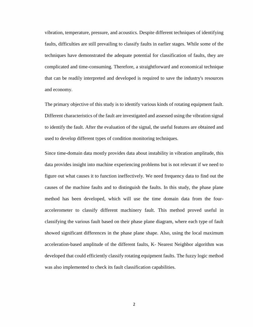
vibration, temperature, pressure, and acoustics. Despite different techniques of identifying

faults, difficulties are still prevailing to classify faults in earlier stages. While some of the

techniques have demonstrated the adequate potential for classification of faults, they are

complicated and time-consuming. Therefore, a straightforward and economical technique

that can be readily interpreted and developed is required to save the industry's resources

and economy.

The primary objective of this study is to identify various kinds of rotating equipment fault.

Different characteristics of the fault are investigated and assessed using the vibration signal

to identify the fault. After the evaluation of the signal, the useful features are obtained and

used to develop different types of condition monitoring techniques.

Since time-domain data mostly provides data about instability in vibration amplitude, this

data provides insight into machine experiencing problems but is not relevant if we need to

figure out what causes it to function ineffectively. We need frequency data to find out the

causes of the machine faults and to distinguish the faults. In this study, the phase plane

method has been developed, which will use the time domain data from the four-

accelerometer to classify different machinery fault. This method proved useful in

classifying the various fault based on their phase plane diagram, where each type of fault

showed significant differences in the phase plane shape. Also, using the local maximum

acceleration-based amplitude of the different faults, K- Nearest Neighbor algorithm was

developed that could efficiently classify rotating equipment faults. The fuzzy logic method

was also implemented to check its fault classification capabilities.

3

1.2 Condition Based Monitoring and Its Necessity

It is desirable to have a minimal level of vibration in the rotating machinery. However,

improper design and malfunction in the machine amplify vibration level. If the machines

are adequately designed, the level of vibration produced by them is minimal. As the

machines are operated continually for more extended periods, they go through wear,

fatigue, and deformation. Once the machine experiences these impacts, the shaft is likely

to be misaligned, and the rotor becomes unbalanced. These faulty scenarios than not only

amplify the vibration level but also supplement the dynamic load on bearings. If the

machines continue to operate with these impacts, it will gradually begin to deteriorate and

may fail catastrophically [1]. The catastrophic failure in the machine will not only halt the

operation of the machine but will also increase the breakdown, decrease productivity, and

economically impact the industries. Although the catastrophic failure is challenging to

avoid, we can at least minimize by observing the machine operating condition which can

be done by observing the machine properties such as vibration, sound, and temperature.

These processes where the machine conditions are observed based on the machine

parameters like vibration, sound, and temperature to avoid any catastrophic failure during

the operation can be termed as condition monitoring [2] [3]. It is crucial to analyze the

modes when dealing with the rotating machinery because of their ability to increase the

vibration. The vibration caused by the rotation should also be studied extensively as these

vibrations tend to amplify without the resonance [4].

As previously mentioned, rotating machinery must be closely monitored using condition

monitoring techniques to warranty its continuous operation. Since condition monitoring

can be carried out based on various machine parameters, several monitoring methods have

4

been used by the industries. Acoustic emission, vibration-based analysis, and infrared

thermography-based monitoring techniques are the most popular and commonly used

condition monitoring techniques in the industry [1]. Maintenance costs are regarded as a

major expense because of their contribution to the general manufacturing of the products.

The equipment requires to be correctly maintained for the manufacturing of the goods,

which includes part replacement, maintenance labor cost and downtime. Overall

maintenance costs vary from industry to industry depending on the type of industry and the

percentage of maintenance costs can be between 15 to 60 percent of the cost of

manufacturing goods. Maintenance requires to be efficiently performed to make it worth

otherwise, it can be counted as an undesirable waste. It is found that an estimated $60

billion is lost owing to inadequate maintenance and poor management, which has a

significant impact on the worldwide competing industries [5]. These reports emphasize the

significance of efficient strategy and management for maintenance in the industries. This

makes condition monitoring an essential tool since a failure to detect machine degradation

has an adverse effect on the monetary side. As the identification of failures and their

translation have been made easier with the accessibility of art and resources of condition

monitoring, it has found for a wide application in the monitoring of machinery [6].

5

1.3 Condition Monitoring Types

1.3.1 Acoustic Emission Based Monitoring Method

As previously mentioned, acoustic emission is one of the industry's conventional

surveillance methods for identifying abnormal behavior of machines. Whenever there is

displacement in the material internal structure strain energy briskly get discharged, which

as a result, generates the elastic stress known as acoustic emission (AE) [7]. The AE signal-

based monitoring technique was proposed by Elijah and Erdal to monitor the cutting tool

as these signals constitute high frequency separating from noise and other unnecessary

sources. The information from the signal sources relating to chip formation and tool wear,

chipping and breakage, formed chip is useful in condition monitoring of the cutting tool.

They used pattern recognition technique and discriminant function for the sources

mentioned above, utilizing the spectral component to extract the feature and make

classification [8]. Acoustic emission saw its enormous rise in the manufacturing industries

for the monitoring of the system because of the sensitivity to the process criterion [9]. If

we combine both vibration and acoustic technique, the result will get better by saving time

and number of workforce required [2].

1.3.2 Infrared Thermography Based Monitoring Method

Infrared thermography is a nondestructive technology that is capable of sensing and

displaying the temperature of machinery components remotely. Using the information of

temperature distribution, fault related to the machinery can be identified [10]. It was seen

that IR technology was capable of sensing the temperature of the skin and could be used

for detecting and diagnosing of the vasospastic disorder. This method was successful in

validating the detection of rheumatology patients during the 1900’s [11]. This technology

6

has found wider application in the field of monitoring the machinery [12] [13] and

evaluating the fatigue limit of the materials [14] [15]. The capabilities of the IR method in

comparison to the vibration monitoring were shown by Lim et al. [16] where the fault

identification accuracy was found comparable to the one using the vibration monitoring.

The advancement in the cameras, along with the easy interpretability of the data makes it

more user-friendly compared to other techniques [2].

1.3.3 Lubricant Analysis Based Monitoring Method

Lubricant analysis is another common monitoring technique where the assessment of

machine is made based on the lubricant samples used. For this method, samples are

examined outside of the machine tested mostly in the laboratory. This technique can

identify the root cause and even detect tiny particles that may influence the future [2].

Although the lubricant analysis is one of the common tools for tracking machines, it has

limitations too. The restriction of this method is on condition monitoring of electrical

devices as it will not be able to deal with these systems. JS Stecki used Ferrographic oil

analysis to predict the failure of jet engines. This technique was capable of detecting wear

particle of all sizes that could provide meaningful information on the characteristics of the

wear particles present in the sample oil used [17]. Flanagan et al. [18] used the lubricant of

steam turbine generator to analyze the presence of wear in the system. If lubricant based

analysis is combined with acoustic emission and vibration analysis technique, the detection

capabilities get more powerful and efficient [19]

1.3.4 Statistical Analysis Based Monitoring Method

Another important condition monitoring tool that addresses a large number of data sets as

temperature data, vibration data, and acoustic signal data is statistical-based analysis. It is

7

possible to apply a statistical method based on the extracted information to classify the

machinery's fault and condition. The different statistical methods are used for fault

detection based on the size of the data set. Poyhonen et al. used Support Vector Machine

(SVM) to classify the fault after making the comparison between Power Spectrum density

with Higher Order Spectra (HOS), Cepstrum Analysis and AR modeling [20]. Lachouri et

al. used Multi-Scale Principal Component Analysis (PCA) so that the cross and auto-

correlation can be selected via PCA and wavelet analysis respectively; the multiscale

Squared Prediction Error (SPE) was then used to identify the faulty condition of the bearing

system [21]. Jiang et al. used the phase space to reconstruct the vibration signal, using the

Phase-PCA based method, the system condition was identified based on the T2 and SPE

value [22]. Harlişca et al. proposed a cheap and user-friendly method for detecting bearing

faults at inceptive stage using statistical processing [23]. Hu et al. used the Ensemble

Empirical Mode Decomposition (EEMD) to decompose the vibration signal into Intrinsic

Mode Functions IMF in order to extract the first five features from IMF, and once the

features were extracted, the SVM was used for the classifying the source data acquired

through the sensor [24]. Li et al. used the Independent Component Analysis (ICA) to

extract the feature and using the reference as the input they used self-organizing-map

(SOM) based neural network to not only detect the fault but also identify the extent of the

fault [25].

1.3.5 Vibration Analysis Based Monitoring Method

Analysis of vibration is regarded as one of the most efficient monitoring technology. When

monitoring the rotating vibration analysis of the equipment, it can be regarded as an optimal

tool as roughly all machines vibrate during their operation. Since the distinct fault generates

8

distinct power at distinct frequencies, vibration assessment is a robust technique that uses

spectrum processing to provide this data in detail [2]. This technique can quickly detect

abrupt changes in the system's conduct. Since it can handle short-term and long-term

surveillance by periodically or permanently mounting the sensor, they are regarded as a

flexible surveillance system. The added advantages for these systems are that vibration

signal can be easily processed using most of the major signal processing methodology

available these days [26]. Vibration analysis has been used successfully to identify the fault

and its types. Using the vibration signal different types of fault corresponding to the bearing

failure, unbalanced caused by mass, misalignment of the shaft, gearbox failure has been

successfully identified. The condition of the machine can be identified using the vibration

signal as it could classify and detect the abnormality in the system [27] [28] [29]. In this

study, Vibration analysis will be used for classifying the fault of rotating machinery

because of its advantages over the other methods which were discussed earlier.

1.3.6 Machine Learning-Based Monitoring Method

The science of machine learning allows the system to understand the program through the

information sets supplied. Since they tend to be feasible and economical, they are widely

used in a broad range of areas such as data mining, computer vision, and pattern recognition

[30]. Recently, several machine-based learning techniques were suggested to identify the

fault and showed strong capacities to detect the fault. Samanta used Artificial Neural

Network (ANN) and Support Vector Machine (SVM) to identify bearing failure. The time-

domain signal was used for features; the signal was optimized using a genetic algorithm to

extract the features. ANN and SVM were used as a classifier for detecting the bearing fault

[31]. Similarly, Jia et al. used the deep learning method for diagnosing the rotating

9

machinery fault where the frequency spectrum was used for training deep learning. Since

the features used were of the frequency spectrum, this method could work with the system

that has a periodical vibrational motion [32]

1.4 Thesis Orientation

The remainder of the thesis chapter will focus on a different model used for identifying and

classifying vibration fault. Chapter II outlines how the raw vibration signal extracted from

the experimental setup is processed for meaningful information. It also provides

information on how different fault conditions are simulated using Machinery Fault

Simulator. Chapter 3 focuses on how the technique of phase plane classification and

detection of vibration failure are implemented. Implementation of fuzzy logic-based fault

classification is addressed in Chapter 4. In addition, Chapter 5 discusses using the K-

Nearest Neighbor model to use the Local Maximum Acceleration-based fault detection

model. Finally, the conclusion of the research and future work will be discussed in Chapter

6.

10

Chapter II

2. Data Analysis and Methodology

2.1 Overview

This chapter focuses on providing a brief outline on how the systems are monitored using

the raw vibration signal. Since the extracted data contains raw information, they need to be

processed further using signal processing to get more meaningful information. This chapter

will provide further information on how an experiment was carried out using the Machinery

setup. It will also provide an idea of what kind of setup is chosen for acquiring and

analyzing data. Moreover, the information on the selection of transducer and signal

processing technique for the experiment is also mentioned. Different methodology that has

been used for the research is also discussed.

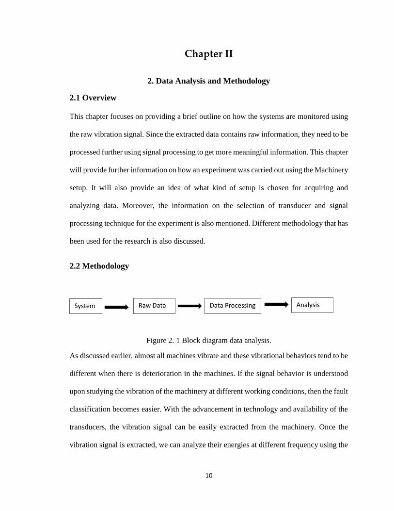
2.2 Methodology

Figure 2. 1 Block diagram data analysis.

As discussed earlier, almost all machines vibrate and these vibrational behaviors tend to be

different when there is deterioration in the machines. If the signal behavior is understood

upon studying the vibration of the machinery at different working conditions, then the fault

classification becomes easier. With the advancement in technology and availability of the

transducers, the vibration signal can be easily extracted from the machinery. Once the

vibration signal is extracted, we can analyze their energies at different frequency using the

System Raw Data Data Processing Analysis

11

spectrum analysis. Since every fault has its own energy for different frequency, the fault

classification using a vibration signal with signal processing method becomes easier. First

step would be acquiring the signal for which we need to mount the transducer in the system.

As there are different types of transducer available in the market, we need to decide the

transducer based on our application and economy.

We must mainly consider in selecting proper transducer and ideal signal processing

methodology based on the application and the system whose parameter is to be measured.

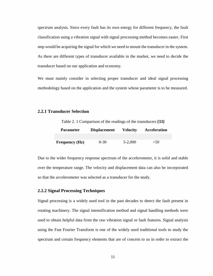
2.2.1 Transducer Selection

Table 2. 1 Comparison of the readings of the transducers [33]

Parameter Displacement Velocity Acceleration

Frequency (Hz) 0-30 5-2,000 >50

Due to the wider frequency response spectrum of the accelerometer, it is solid and stable

over the temperature range. The velocity and displacement data can also be incorporated

so that the accelerometer was selected as a transducer for the study.

2.2.2 Signal Processing Techniques

Signal processing is a widely used tool in the past decades to detect the fault present in

rotating machinery. The signal intensification method and signal handling methods were

used to obtain helpful data from the raw vibration signal or fault features. Signal analysis

using the Fast Fourier Transform is one of the widely used traditional tools to study the

spectrum and certain frequency elements that are of concern to us in order to extract the

12

characteristic features. These methods are based on the frequency analysis that has some

limitation on the side. As it assumes the signal being linear and stationary, they are unable

to deal with the time localized transient events which are of the non-stationary nature.

Hence, we are unable to get the information of the vibration in time domain, making us

difficult to find when the machine fault occurs [34] [35]. To overcome these limitations,

the time – frequency analysis approach got started. The time–frequency analysis techniques

such as Short-Term Fourier Transform (STFT) [36], Wigner-Ville Distribution (WVD)

[37] [38] showed the capabilities of the handling the non-stationary signals but they also

have some limitations as STFT can only deal with the transient signal which dynamics

changes slowly as they are based on the signal segmentation. WVD which are not based

on the segmentation do overcome the limitation of the STFT, but they also have a limitation

as the inference term formed by the transformation makes it harder to understand the

estimated distribution. The signal based on the Wavelets came into the practice to

overcome these difficulties known as Wavelet Transform (WT) [39] [40], which depicted

the signal in time scale rather than time-frequency representation. The development of the

wavelet Transform has led to the technique of continuous Wavelet Transform (CWT) [41]

and discrete Wavelet Transform (DWT). These techniques have been successful in dealing

with the fault detection of non-stationary signals. In this work, FFT and CWT have been

used for the processing of the vibration data. FFT has been used for the feature extraction

purpose for the fuzzy logic-based method for classifying unbalanced and misalignment

condition present in the machinery.

13

2.2.3 Experimental Setup

Machinery Fault Simulator (MFS) as seen in Figure 2.2, was used for simulating the

different working condition of the machine. This is a powerful simulating tool capable of

simulating numerous machinery fault condition.

Figure 2. 2 Machinery fault simulator setup

Figure 2. 3 Accelerometer positioning

a1

a2

a4

a3

14

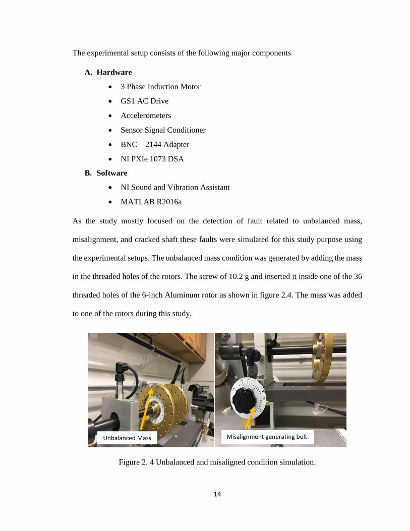
The experimental setup consists of the following major components

A. Hardware

3 Phase Induction Motor

GS1 AC Drive

Accelerometers

Sensor Signal Conditioner

BNC – 2144 Adapter

NI PXIe 1073 DSA

B. Software

NI Sound and Vibration Assistant

MATLAB R2016a

As the study mostly focused on the detection of fault related to unbalanced mass,

misalignment, and cracked shaft these faults were simulated for this study purpose using

the experimental setups. The unbalanced mass condition was generated by adding the mass

in the threaded holes of the rotors. The screw of 10.2 g and inserted it inside one of the 36

threaded holes of the 6-inch Aluminum rotor as shown in figure 2.4. The mass was added

to one of the rotors during this study.

Figure 2. 4 Unbalanced and misaligned condition simulation.

Misalignment generating bolt. Unbalanced Mass

15

Similarly using the Alignment Jack Bolt, the misalignment condition was generated. Using

the Alignment Jack bolt, the system can be misaligned to the desirable milli-inch (mils) as

seen in the dial indicator. Using the misalignment generating bolt the angular misalignment

condition is simulated in the system by 5 mils and 10 mils.

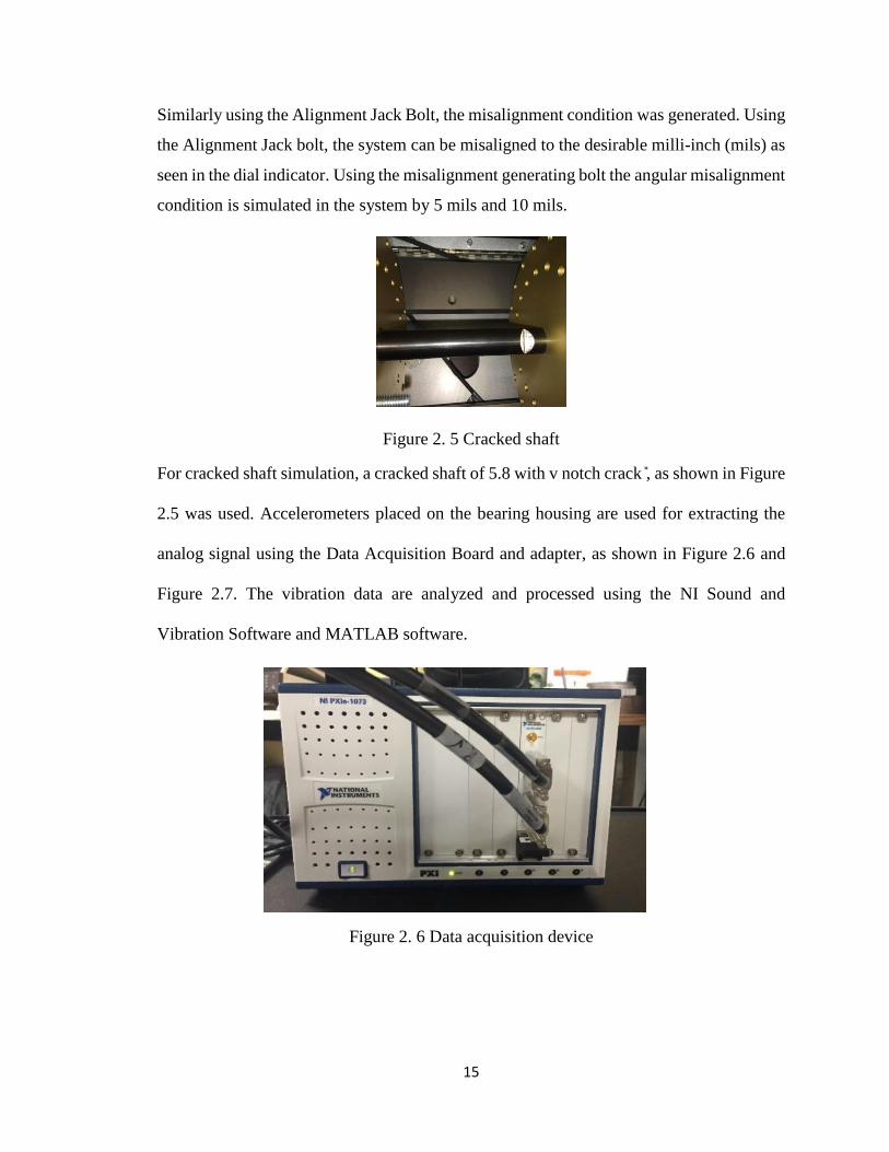
Figure 2. 5 Cracked shaft

For cracked shaft simulation, a cracked shaft of 5.8 with v notch crack ̎, as shown in Figure

2.5 was used. Accelerometers placed on the bearing housing are used for extracting the

analog signal using the Data Acquisition Board and adapter, as shown in Figure 2.6 and

Figure 2.7. The vibration data are analyzed and processed using the NI Sound and

Vibration Software and MATLAB software.

Figure 2. 6 Data acquisition device

16

Figure 2. 7 Adapter

2.2.4 Methods Used for Classifying the Vibration Fault

Fuzzy Inference system has been used to classify the fault and its severity in which the

amplitude and frequencies are taken as the input for developing a fuzzy inference system.

With the formulation of rule based on the triangular membership function, the model is

developed which will provide an output on the condition of the machine and severity level

in the case of fault presence. Further Phase plane diagram-based method is proposed for

the classification of the fault and its type based on the unique characteristics shown by the

different faulty condition along with the healthy condition. Here, the vibration response of

all the 4-accelerometers attached to the bearing housing are plotted against each other and

their behavior are noted. The flow diagram used for the data analysis is shown in the below

figure 2.8

17

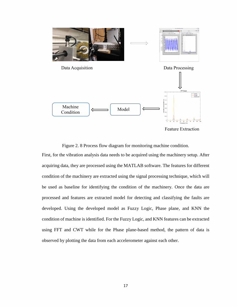
Figure 2. 8 Process flow diagram for monitoring machine condition.

First, for the vibration analysis data needs to be acquired using the machinery setup. After

acquiring data, they are processed using the MATLAB software. The features for different

condition of the machinery are extracted using the signal processing technique, which will

be used as baseline for identifying the condition of the machinery. Once the data are

processed and features are extracted model for detecting and classifying the faults are

developed. Using the developed model as Fuzzy Logic, Phase plane, and KNN the

condition of machine is identified. For the Fuzzy Logic, and KNN features can be extracted

using FFT and CWT while for the Phase plane-based method, the pattern of data is

observed by plotting the data from each accelerometer against each other.

Data Acquisition Data Processing

Feature Extraction

Model Machine

Condition

18

Chapter III

3. Phase Plane Diagram Based Method for Fault Classification

3.1 Overview

Through this chapter, a novel method for detecting and classifying fault related to

misalignment, cracked shaft, and unbalanced mass will be presented. This simple and user-

friendly tool using the four-accelerometer data can classify the fault as all these operating

conditions of the machine shows distinctive characteristic.

3.2 Phase Plane Diagram

Phase plane diagram is the simple representation of the vibration signal measured from all

the accelerometer plotted against each other. Vibration data acquired from the

accelerometer a1, a2, a3, and a4 located along horizontal and vertical directions are cross-

compared using this method. For this study purpose the data from these accelerometers

will be represented as shown in the table 3.1 below.

Table 3. 1 Position and representation of the accelerometer

Accelerometer Position Representation

1 Vertical Left VL

2 Horizontal Left HL

3 Horizontal Right HR

4 Vertical Right VR

a3

19

3.2.1 Phase Plane Diagram for Healthy and Misaligned Data

The vibration signal data of all four accelerometers were plotted against each other for

three different data sets. The operating speed of the machinery was 20 Hz while for the

misaligned condition the misalignment levels were 5 mils and 10 mils respectively. Once

they were plotted, they were cross-compared. The plot is illustrated in Figure 3.1 from

Healthy data set and can be seen that the plane drawn are represented in the Horizontal

shape for all the six plots.

Figure 3. 1 Healthy dataset phase plane diagram (20 Hz)

Now, it was also interesting to see how the phase plane diagram represents when the system

is subjected to 5mils (5 milli inch) angular misalignment and operated at 20 Hz.

20

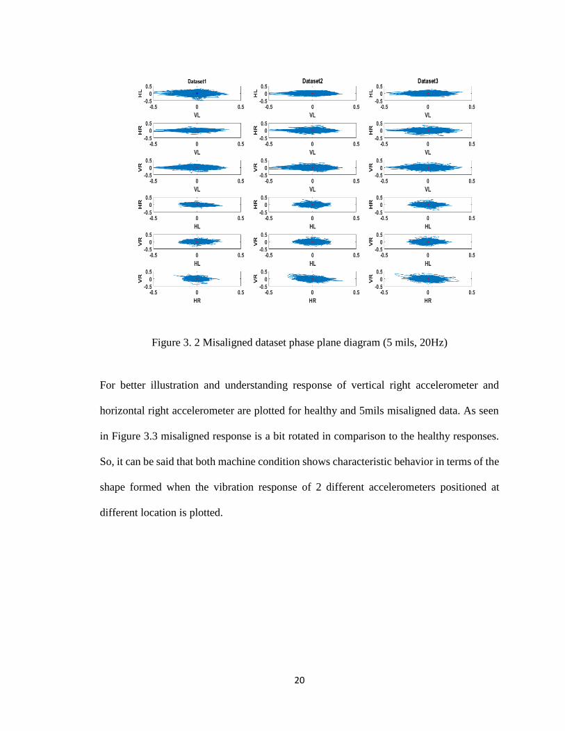
Figure 3. 2 Misaligned dataset phase plane diagram (5 mils, 20Hz)

For better illustration and understanding response of vertical right accelerometer and

horizontal right accelerometer are plotted for healthy and 5mils misaligned data. As seen

in Figure 3.3 misaligned response is a bit rotated in comparison to the healthy responses.

So, it can be said that both machine condition shows characteristic behavior in terms of the

shape formed when the vibration response of 2 different accelerometers positioned at

different location is plotted.

21

Figure 3. 3 Healthy vs misaligned (5 mils) comparison

When the phase plane diagram for the healthy and misaligned data are plotted individually,

there appears to be a considerable difference in the phase plane shape. The phase plane plot

of the vertical right and horizontal right from figure 3.3 shows the shift in the phase shape

from its reference line. There is not a huge difference in the shape of healthy and misaligned

data but there are considerable differences.

3.2.2 Phase Plane Diagram for Unbalanced Data

Similarly, it was checked what difference it makes when the condition of the machine is

switched to the unbalanced state. Looking at the figure 3.4, it can be noticed that the shape

of the plane diagram shows differences in the shape formation.

22

Figure 3. 4 Unbalanced dataset phase plane diagram (20 Hz)

Further, the most significant shape was plotted which is for vertical right vs horizontal right

to make better illustration that can be seen in Figure 3.5.

Figure 3. 5 Healthy vs unbalanced comparison

23

Whenever there is a presence of the unbalanced mass cross response between the

accelerometer positioned at the horizontal left, and horizontal right are distinctive in shape.

The shape rotates on the right side or there is rotational movement. It can be noticed that

unbalanced condition has a significant effect on the response than the misaligned condition

this could be because of the misalignment generated at the left end of the machinery.

3.2.3 Phase Plane Diagram for Cracked Shaft Data

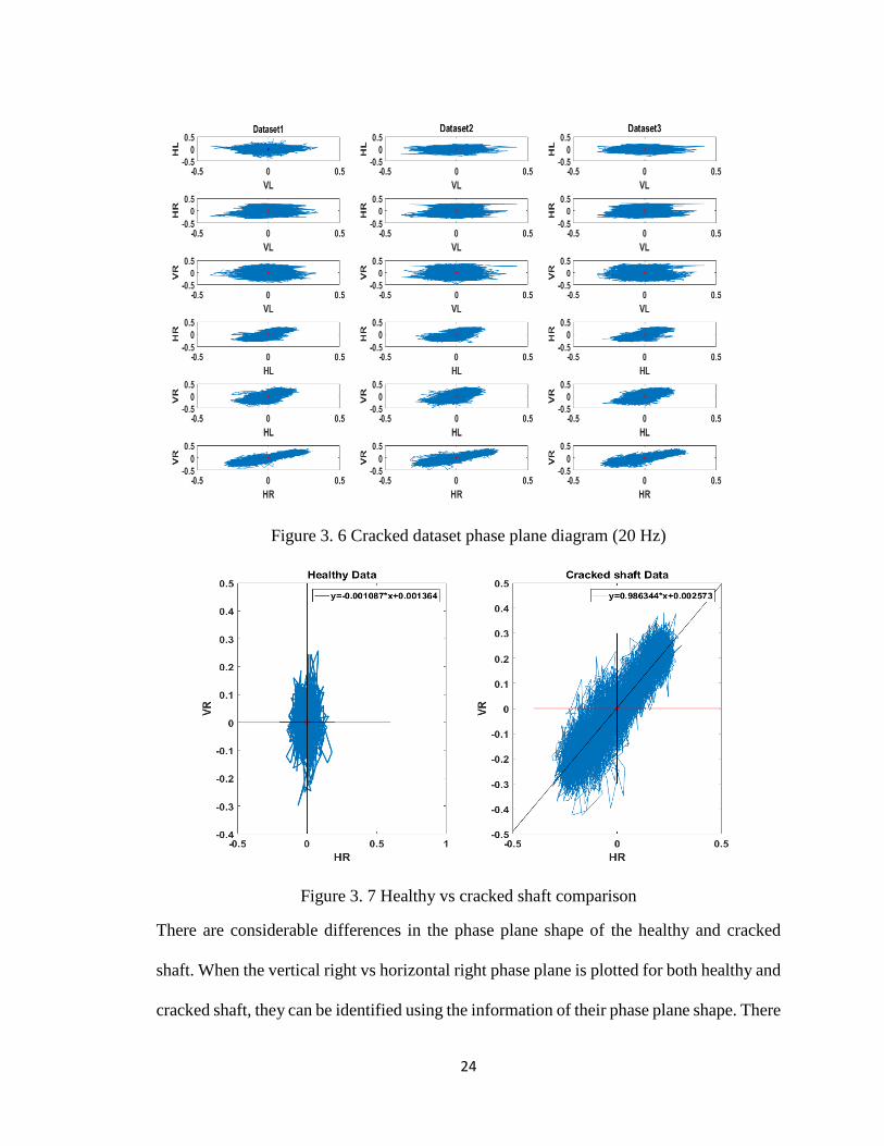
Further, the phase plane diagram for the condition with cracked shaft is plotted to see the

behavior or the characteristics of this condition. Like the above-mentioned condition 3,

data sets of cracked condition machine operating at 20 Hz is plotted. As seen in Figure 3.6

it can be observed that the shape of the plot for the cracked data set is entirely different

when the accelerometer data of (HR, HL), (VR, HL) and (HR, VR) are plotted. The shape

of cracked data is rotated as compared to the healthy data set. The HR accelerometer data

is plotted against VR data for further illustration and clarity in Figure 3.7.

24

Figure 3. 6 Cracked dataset phase plane diagram (20 Hz)

Figure 3. 7 Healthy vs cracked shaft comparison

There are considerable differences in the phase plane shape of the healthy and cracked

shaft. When the vertical right vs horizontal right phase plane is plotted for both healthy and

cracked shaft, they can be identified using the information of their phase plane shape. There

25

is significant shift in the shape of the vertical right vs horizontal right plot when the system

has cracked shaft condition. The distribution of data and chaotic behavior of the machine

under different operating condition makes data distribution and phase plane diagram

distinctive.

Chapter Summary

With the data from all four accelerometers that were recording the horizontal and vertical

vibration motion of the machinery are analyzed and plotted against each other to see if they

show any distinctive pattern. The phase plane diagram of these accelerometers when

plotted showed a distinctive pattern where different fault condition showed different

behavior. Using the phase plane diagram, we were able to find the fault pattern of the

different operating condition of the rotating machinery. Healthy, misaligned, unbalanced,

and cracked shaft condition were distinctive when the accelerometer data of (HR, HL),

(VR, HL), and (HR, VR) were plotted. These phase plane diagram can be used as a baseline

for identifying the working condition of the machine. This method is simple and

economical to be implemented so it can be a great asset to the industry. Further, the reason

behind the differences in these particular directions of vibration is to be studied and

analyzed.

26

Chapter IV

4. Fuzzy Logic-Based Fault Classification Method

4.1 Introduction

In this chapter, the effectiveness of fuzzy logic in classifying the vibration fault present in

the rotating machinery will be discussed. This economical and straightforward tool which

is easy to develop and interpret was used to classify the unbalanced and misalignment fault

present in the machinery.

Traditional logic is based on the Boolean logic that satisfies the principle of bivalence

where the logic is based on either true or false simply represented as 1 and 0. Fuzzy logic,

on the other hand, is a multivalued logic based on the degree of multiple truths expressed

on the closed interval [0, 1] by the values.

In Fuzzy Logic, the 0 and 1 are associated with traditional False and True Value,

respectively. Fuzzy logic represents the variation of truth’s degree in terms of the value (0,

1). There are numerous ways to express the Fuzzy operation but for our easiness, it will be

discussed in an uncomplicated way. For the given fuzzy values of x and y the following

operations can be defined [42].

(𝒙 𝒂𝒏𝒅 𝒚) = 𝐦𝐢𝐧 (𝒙, 𝒚) (4.1)

(𝒙 𝒐𝒓 𝒚) = 𝐦𝐚𝐱 (𝒙, 𝒚) (4.2)

(𝒏𝒐𝒕 𝒙) = 𝟏 − 𝒙 (4.3)

27

(𝒙 𝒊𝒎𝒑𝒍𝒊𝒆𝒔 𝒚) = 𝐦𝐚𝐱 (𝒙, 𝟏 − 𝒚) (4.4)

If the above definition is considered as traditional logic, then the Truth and False value

would be expressed as 1 and 0, respectively. If we have to define the Fuzzy set, we try to

represent it as a universe of discourse where the function S represents the membership

function of the fuzzy set [42]

𝝁𝑺:𝑼 → [𝟎, 𝟏] (4.5)

Since the universal set of real numbers R is restricted, so the membership function is

represented as:

𝝁𝑺:𝑹 → [𝟎, 𝟏] (4.6)

The finite set are then restricted to the fuzzy subsets. The Fuzzy set S operator (∈) can be

defined as: [42]

(𝒙 ∈ 𝑺) = 𝝁𝑺(𝒙) (4.7)

Hence, the set of fuzzy S returns the true and false value. If the right- hand side is a fuzzy

set, then the value returned is no longer a Boolean operator. If we have two fuzzy sets T

and S, we define the membership functions of S ∪ T, S ∩ T and S´ as:

μ(S∪T)(x)=(μS(x)or μT(x)) =max(μS(x),μT(x)) (4.8)

μ(S∩T)(x)=(μS(x) and μT(x)) =min(μS(x),μT(x)) (4.9)

28

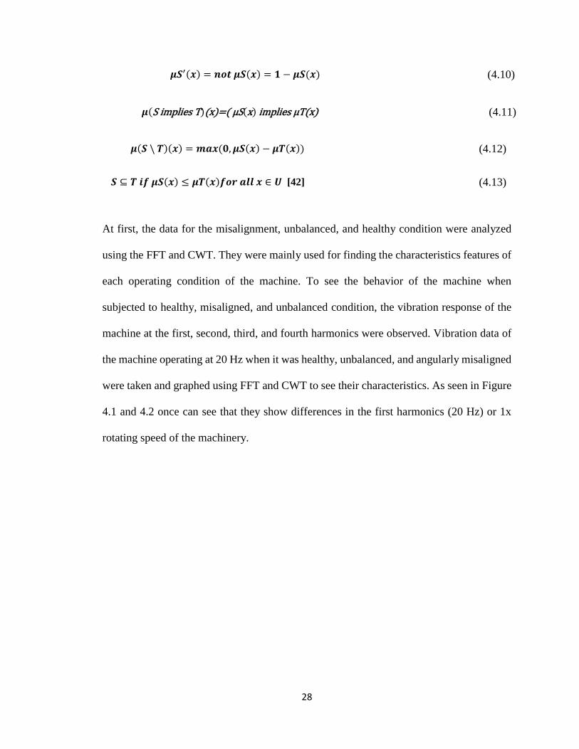
𝝁𝑺′(𝒙) = 𝒏𝒐𝒕 𝝁𝑺(𝒙) = 𝟏 − 𝝁𝑺(𝒙) (4.10)

𝝁(S implies T)(x)=( μS(x) implies μT(x) (4.11)

𝝁(𝑺 \ 𝑻)(𝒙) = 𝒎𝒂𝒙 (𝟎, 𝝁𝑺(𝒙) − 𝝁𝑻(𝒙)) (4.12)

𝑺 ⊆ 𝑻 𝒊𝒇 𝝁𝑺(𝒙) ≤ 𝝁𝑻(𝒙)𝒇𝒐𝒓 𝒂𝒍𝒍 𝒙 ∈ 𝑼 [42] (4.13)

At first, the data for the misalignment, unbalanced, and healthy condition were analyzed

using the FFT and CWT. They were mainly used for finding the characteristics features of

each operating condition of the machine. To see the behavior of the machine when

subjected to healthy, misaligned, and unbalanced condition, the vibration response of the

machine at the first, second, third, and fourth harmonics were observed. Vibration data of

the machine operating at 20 Hz when it was healthy, unbalanced, and angularly misaligned

were taken and graphed using FFT and CWT to see their characteristics. As seen in Figure

4.1 and 4.2 once can see that they show differences in the first harmonics (20 Hz) or 1x

rotating speed of the machinery.

29

Figure 4. 1 FFT graph for healthy, misaligned and unbalanced data

Figure 4. 2 CWT graph for healthy and unbalanced data

30

The triangular membership function is used for mapping the input points to the respective

membership value (0-1). If X represents the universe of discourse and x represents its

element, then the fuzzy set A in x can be defined as the ordered pair sets [43].

𝑨 = {𝒙, µ𝑨(𝒙)| 𝒙 ∈ 𝑿} (4.14)

where µ𝐴(𝑥) is the membership function.

The triangular membership function used for defining the membership function of the input

can be defined mathematically as below:

𝐟(𝐱; 𝐚, 𝐛 𝐜) =

{

𝟎 𝒙 ≤ 𝒂𝒙−𝒂

𝒃−𝒂 𝒂 ≤ 𝒙 ≤ 𝒃

𝒄−𝒙

𝒄−𝒃 𝒃 ≤ 𝒙 ≤ 𝒄

𝟎 𝒙 ≥ 𝒄

(4.15)

where a, b, and c are the scalar parameter on which triangular curve is dependent. Once the

membership function for the input parameters are defined the 9 rule sets are defined based

upon which the Fuzzy Interface will provide its output. These rules are used to evaluate the

condition of the machine

After the vibration data is measured using the accelerometer signal under the normal and

faulty conditions then the spectrum pattern is obtained by using the FFT. The healthy and

faulty data sets obtained are then further analyzed to extract the features. These features

are used as a baseline to classify the faults using the fuzzy System. The fuzzy system takes

vibration amplitude and frequency as its input variables while the output for the system

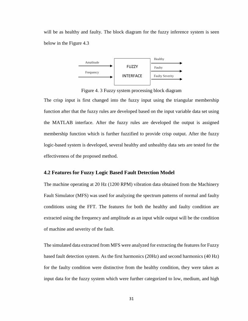
31

will be as healthy and faulty. The block diagram for the fuzzy inference system is seen

below in the Figure 4.3

Figure 4. 3 Fuzzy system processing block diagram

The crisp input is first changed into the fuzzy input using the triangular membership

function after that the fuzzy rules are developed based on the input variable data set using

the MATLAB interface. After the fuzzy rules are developed the output is assigned

membership function which is further fuzzified to provide crisp output. After the fuzzy

logic-based system is developed, several healthy and unhealthy data sets are tested for the

effectiveness of the proposed method.

4.2 Features for Fuzzy Logic Based Fault Detection Model

The machine operating at 20 Hz (1200 RPM) vibration data obtained from the Machinery

Fault Simulator (MFS) was used for analyzing the spectrum patterns of normal and faulty

conditions using the FFT. The features for both the healthy and faulty condition are

extracted using the frequency and amplitude as an input while output will be the condition

of machine and severity of the fault.

The simulated data extracted from MFS were analyzed for extracting the features for Fuzzy

based fault detection system. As the first harmonics (20Hz) and second harmonics (40 Hz)

for the faulty condition were distinctive from the healthy condition, they were taken as

input data for the fuzzy system which were further categorized to low, medium, and high

FUZZY

INTERFACE Faulty Severity

Frequency

Healthy

Faulty Amplitude

32

value. The amplitude (g) of the first and second harmonics were extracted from 20

combining data sets of healthy and faulty data which were then used as the features to

separate these condition as shown in Tables 4.1 and 4.2 below.

First, the features were extracted for healthy and unbalanced Data. The features selected

were the amplitude of the first and second harmonics calculated in terms of g.

33

Table 4. 1 Features of healthy and unbalanced data

S.N 1st

Harmonics

2nd

Harmonics

Machine Status

1 0.010364 0.006439 Healthy

2 0.010168 0.006362 Healthy

3 0.009664 0.005858 Healthy

4 0.009762 0.008135 Healthy

5 0.009259 0.005932 Healthy

6 0.008918 0.006652 Healthy

7 0.009079 0.007359 Healthy

8 0.00904 0.008271 Healthy

9 0.008911 0.006928 Healthy

10 0.008933 0.00826 Healthy

11 0.128761 0.003766 Unbalanced

12 0.127431 0.002573 Unbalanced

13 0.127759 0.004255 Unbalanced

14 0.12657 0.001911 Unbalanced

15 0.125938 0.003444 Unbalanced

16 0.125597 0.003682 Unbalanced

17 0.125143 0.002388 Unbalanced

18 0.124651 0.002035 Unbalanced

19 0.124536 0.002566 Unbalanced

20 0.12474 0.00262 Unbalanced

As seen in the above Table 4.2, the features from the 20 data sets are selected and there

seems to be the significant difference in the 1st and 2nd harmonic amplitudes when the

operating condition of the machinery is abnormal compared to normal and further, the 1st

harmonic amplitude for the Unbalanced condition if greater than that of Normal operating

34

condition. Similarly, the system was subjected to the misaligned condition and features of

the 1st and 2nd harmonics were calculated as shown in the Table 4.2 below

Table 4. 2 Features of healthy and misaligned data

S.N 1st

Harmonics

2nd

Harmonics

Machine Status

1 0.027 0.0042 Misaligned

2 0.0269 0.0069 Misaligned

3 0.0267 0.0063 Misaligned

4 0.0269 0.0042 Misaligned

5 0.0268 0.0038 Misaligned

6 0.0268 0.0057 Misaligned

7 0.0266 0.0051 Misaligned

8 0.0265 0.0051 Misaligned

9 0.0266 0.0057 Misaligned

10 0.0263 0.0049 Misaligned

11 0.010364 0.006439 Healthy

12 0.010168 0.006362 Healthy

13 0.009664 0.005858 Healthy

14 0.009762 0.008135 Healthy

15 0.009259 0.005962 Healthy

16 0.008918 0.006652 Healthy

17 0.009079 0.007359 Healthy

18 0.00904 0.008271 Healthy

19 0.008911 0.006928 Healthy

20 0.008933 0.00826 Healthy

After feature extraction, the Fuzzy Logic tool box was used to generate the Fuzzy Interface

System (FIS) to classify the fault. After developing the fuzzy-based fault detection

35

interface based on the 9 rules, the test data set of both healthy and unbalanced condition

were tested for its effectiveness. The machine is in faulty or unhealthy condition if the FIS

value is greater than 0.5 and larger the value of FIS, greater is the severity.

4.3 Results

Using the fuzzy logic toolbox of MATLAB (version: R 2016a) fault classification model

was developed. The acceleration amplitude (g) and the frequency were chosen as input for

the proposed fuzzy model. Then triangular membership function was used for assigning

the membership value for the three operating conditions of the machinery. The membership

value was chosen as low, medium and high based on the acceleration amplitude operating

conditions. After assigning the membership function, the nine fuzzy rules were used for

classifying and identifying the severity of the machine operating condition. Based upon the

membership function and rules, the fuzzy model could give output as Healthy, Unbalanced

and Misaligned. Also, the FIS value would provide an insight on the severity level of the

machine operating condition.

First healthy and unbalanced unknown data set were tested using the proposed fuzzy logic

model. It could easily classify the normal and misaligned working condition of the

machinery. As seen in the Table 4.3, healthy and unbalanced condition are classified

accurately.

36

Table 4. 3 Features of healthy and unbalanced data

S.N 1st

Harmonics

2nd

Harmonics

Machine

Status

FIS Results

1 0.008197 0.006302 Healthy 0.3667

2 0.00898 0.007254 Healthy 0.35813

3 0.008437 0.006239 Healthy 0.36376

4 0.008695 0.006407 Healthy 0.37254

5 0.008426 0.00721 Healthy 0.35962

6 0.008559 0.008009 Healthy 0.33352

7 0.008612 0.006933 Healthy 0.37363

8 0.008192 0.008138 Healthy 0.33159

9 0.008332 0.006184 Healthy 0.36103

10 0.008084 0.006698 Healthy 0.38629

11 0.125155 0.001756 Unbalanced 0.6615

12 0.124891 0.002249 Unbalanced 0.66113

13 0.124458 0.003556 Unbalanced 0.61689

14 0.124739 0.002312 Unbalanced 0.66091

15 0.124596 0.001919 Unbalanced 0.6607

16 0.124661 0.002661 Unbalanced 0.65448

17 0.124384 0.001273 Unbalanced 0.65836

18 0.124487 0.002994 Unbalanced 0.64053

19 0.124164 0.002527 Unbalanced 0.65907

20 0.12413 0.002591 Unbalanced 0.65696

Based on the threshold of 0.5, FIS above 0.5 is identified as an unbalanced condition while

below 0.5 is identified as a normal operating condition. Also, based on the FIS value, the

severity of the machine can be identified. The greater the FIS value higher the severity of

the machinery. Since the unbalanced operating condition is more severe compared to

37

healthy operating condition, the FIS value is relatively higher for it. As can be seen from

Table 4.3, the Fuzzy inference system could distinguish between the unbalanced and

healthy operating condition of the machine based on the threshold of FIS value. As the

unbalanced condition is more severe than the healthy operating condition, the severity

results obtained from the FIS validates the statement. This simple technique can be thus

utilized to detect the unbalanced fault.

Similarly, the fuzzy model was tested for the classification capabilities of misalignment

and healthy operating condition. Twenty unknown data set were tested using the proposed

fuzzy model. As seen in Table 4.4, the model could classify the normal and misaligned

operating condition of the machine with distinction. Similar to the proposed model for

unbalanced condition, it could identify the machine operating condition severity. Based on

the threshold of 0.5 FIS above 0.5 is identified as a misaligned condition while below 0.5

is identified as a normal operating condition. The severity can be identified based on the

FIS value, where greater the FIS value higher the severity.

38

Table 4. 4 Features of healthy and misaligned data

S.N 1st

Harmonics

2nd

Harmonics

Machine

Status

FIS

Results

1 0.0262 0.0049 Misaligned 0.62861

2 0.0264 0.0066 Misaligned 0.64666

3 0.0264 0.0046 Misaligned 0.62144

4 0.0263 0.0072 Misaligned 0.61734

5 0.0265 0.0052 Misaligned 0.6451

6 0.0265 0.0048 Misaligned 0.62085

7 0.0266 0.0054 Misaligned 0.64875

8 0.0265 0.0065 Misaligned 0.6477

9 0.0266 0.0046 Misaligned 0.62085

10 0.0268 0.006 Misaligned 0.65057

11 0.009 0.0073 Healthy 0.4133

12 0.0084 0.0062 Healthy 0.36489

13 0.0087 0.0064 Healthy 0.37211

14 0.0084 0.0072 Healthy 0.40525

15 0.0086 0.008 Healthy 0.36824

16 0.0086 0.0069 Healthy 0.40317

17 0.0082 0.0081 Healthy 0.35856

18 0.0082 0.0063 Healthy 0.35869

19 0.0083 0.0062 Healthy 0.36211

20 0.0081 0.0067 Healthy 0.37648

Using the features of first and second harmonics, the unbalanced and misalignment fault

can be distinguished with healthy operating machine condition. The proposed method was

developed separately for classifying healthy condition with the misaligned and unbalanced

39

condition. In the future, these three faults can be incorporate together and classified along

with their severity level.

Chapter Summary

In this chapter, the fault detection method for rotating machinery was purposed. Initially

the most important features are identified using the FFT or CWT. The FFT is chosen. The

features selected were the amplitude of the first and second harmonics for the normal and

abnormal working conditions. After selecting the features, the fuzzy inference system was

modeled using the MATLAB (version: R 2016a). The triangular membership function was

chosen for mapping the degree of membership. After developing the Fuzzy system, they

were tested on the extracted features. The fuzzy logic-based method showed good fault

detection capabilities. It could not only easily identify healthy, unbalanced, and misaligned

condition of the machinery, but also the severity of the machine based on the FIS level. As

this method is easy to interpret and develop, it could be a useful tool in the industry.

40

Chapter V

5. Local Maximum Acceleration Based Rotating Machinery Fault

Classification Using KNN

5.1 Introduction

Industries such as process, oil, and gas have widely deployed rotating machinery. To operate

continuously at the optimum level, these industries need rotating machinery. These

machines overall performance depends largely on the condition of their components such

as bearings, seals, gearboxes, pumps, compressors, motors, and generators. Absence of a

practical monitoring approach could cause a machine, and its part to fail catastrophically.

Industries aim not only to minimize the failure rate of machines but also to optimize their

maintenance resource. Taking maintenance action only when there is an abnormality in the

operation of the machinery helps industries to get rid of additional cost incurred due to

irrelevant schedule maintenance. CBM is considered as one of the most comprehensive

monitoring and maintenance approaches because of its ability to optimize maintenance

resources, minimize the risk of catastrophic failure, and improve machine reliability [34].

The CBM technique is based on various machine parameters such as temperature, vibration,

and sound to determine the operating condition of the machine [2]. Vibration parameter

based monitoring has proven to be a strong tool for identifying and detecting different fault

such as bearing failure, misalignment, and unbalance in the rotating machinery [44] [45].

Since most rotating machines vibrate during their operation and different faults produce

distinctive energy at a particular frequency, vibration-based monitoring can be considered

41

as an ideal tool for detecting and identifying the machines faults [2]. Usually, the vibration-

analysis is based on time and frequency domain methods. For analyzing vibration signal in

time domain amplitude is taken as a function of time while for frequency domain analysis

amplitude is considered as a function of frequency. The most common vibration fault like

bearing failure can be predicted and detected using the vibration signal [46].

Machine learning (ML) is the science that empowers the intelligence of a machine to learn

program by using example data and prior understanding [47]. ML is gaining popularity

these days because of their agility to adapt to unfamiliar scenarios and capability of solving

the complicated tasks that are difficult to be solved using mathematical modeling [48]. ML

approaches such as Artificial Neural Network (ANN), Support Vector Machine (SVM),

Deep Learning, Hidden Markov Model (HMM) has successfully identified faults in

rotating machinery and their capabilities are still yet to exploit in various rotating

machinery applications [49] [50] [32]. Pandya et al. used a modified KNN algorithm built

on asymmetric proximity function (APF) to classify rolling element bearing fault. They

used acoustic emission data for fault classification of rolling element bearing, and the result

showed very good accuracy of 96.67% [51]. Lei and Zuo used weighted K-Nearest

Neighbor to identify the crack level of gears. To detect gear damage and characterize gear

condition, the time and frequency domain features of gear subjected to different load and

rotor speed were used. The identification of the crack level of gears using this approach

was found to be satisfactory [52]. Using the acceleration amplitude of 1x to 6x rotational

speed as a feature, Nejadpak and Yang proposed a KNN based algorithm. This method

showed satisfactory fault classification capability with an accuracy of 95% [53]. By

analyzing the operating frequencies and their harmonics, various machine malfunctions

42

caused by rotor imbalance and shaft misalignment are predicted and detected. It has been

observed from the earlier literature work that operating frequencies and their harmonics

have been used primarily to detect, classify, and predict machine faults. At these

frequencies and their harmonics, preeminent differences are expected to occur. Although

dominant differences may be observed at one time (1x) operating speed, it may not be

accurate with other harmonic speed. The study then tried to check whether these dominant

peaks or dominant acceleration amplitude are exactly located at the operational frequencies

and their harmonics. So, the acceleration amplitude of harmonic frequencies and local

maximum acceleration amplitude were determined. Finally, these amplitudes of

acceleration were compared to test their similarity. It was found that besides a few

amplitudes of acceleration rest others were not the same. It was evidential that acceleration

amplitude of the harmonic frequencies and the maximum local acceleration were not

identical. It could be misleading to use acceleration amplitude features at operating speed

and its harmonics only, so the maximum local acceleration amplitude and acceleration

amplitude at operating speed were selected as a vibration feature for the proposed KNN

classifier.

5.2 Methodology

KNN is a simple supervised learning algorithm used for separating the data points into

different classes. This nonparametric classification algorithm assigns the non-descriptive

test samples to the particular class based on the measurement of the distance to the nearest

training samples [54]. Easy interpretability without training requirement makes this method

straightforward. The effectiveness of the algorithm is based on the suitable selection of the

nearest neighbors.

43

The training data set can be represented as 𝑇 = {(𝑥1, 𝑦1),… , (𝑥𝑛, 𝑦𝑛)}. Here, 𝑥𝑖 is the n-

dimensional feature vector and 𝑦𝑖 the corresponding class level. The binary classes are

labeled as 0 or 1. KNN constructs a logical sub-region 𝑅(𝑥) ⊆ ℜ𝑑 from the training set at

the estimation point x. The region is predicted based on the following criterion [55]

𝑹(𝒙) = {�̂�|𝑫(𝒙, �̂� ) ≤ 𝒅(𝒌)} (5.1)

Where 𝐷(𝑥, �̂� ) is a distance metric, and 𝑑(𝑘) is the kth order statistic of {𝐷(𝑥, �̂�)}1𝑛. The

number of samples in R(x) is denoted by 𝑘 [𝑦]. The posterior probability 𝑝(𝑦 𝑥) of 𝑥 is

obtained as:

𝒑(𝒚 𝒙) =𝒑(𝒙 𝒚)𝒑(𝒚)

𝒑(𝒙)≅

𝒌[𝒚]

𝒌 5.2

The decision 𝑔(𝑥) is obtained from the highest 𝑘[𝑦] value

𝒈(𝒙) = {𝟏, 𝒌[𝒚 = 𝟏] ≥ 𝒌[𝒚 = 𝟎],

𝟎, 𝒌[𝒚 = 𝟎] ≥ 𝒌[𝒚 = 𝟏]. 5.3

The KNN algorithm allocates a class from the decision with maximum posterior probability.

The decision rule for binary classification 𝑦𝑖 ∈ {0, 1} can be simplified as 𝒈(𝒙) =

𝒔𝒈𝒏(𝒂𝒗𝒆𝒙𝒊 ⋲𝑹(𝒙)𝒚𝒊)

The KNN algorithm was used for classifying misalignment, and unbalanced fault as they

are the most common cause of the rotating machinery failure. The local maximum

acceleration amplitude and its location were initially identified for healthy, misaligned and

unbalanced conditions. For the above-mentioned operating conditions, their local maximum

acceleration amplitude information was extracted. These extracted characteristics were

chosen as vibration features for the proposed KNN classification. The Euclidean distance

function was used to calculate the distance of the test sample from a training sample. The

44

number of k was selected as three based on the number of classes and the training set. Since

the KNN result depends on the selected value of k, Euclidean distance is built in the same

class to compensate for the error caused by the incorrect selection of k.

The characteristics of the normal, misaligned and unbalanced condition were analyzed using

Fast Fourier Transform (FFT) in the MATLAB (version: R2016a) after acquiring the signal

from the Machinery Fault Simulator (MFS). Also, to extract substantial information, the

local maxima for the different operating conditions were identified and graphed. Several

data sets were studied for the comparative study of healthy, misaligned and unbalanced

condition to gather more information about the most common and dominant local maxima.

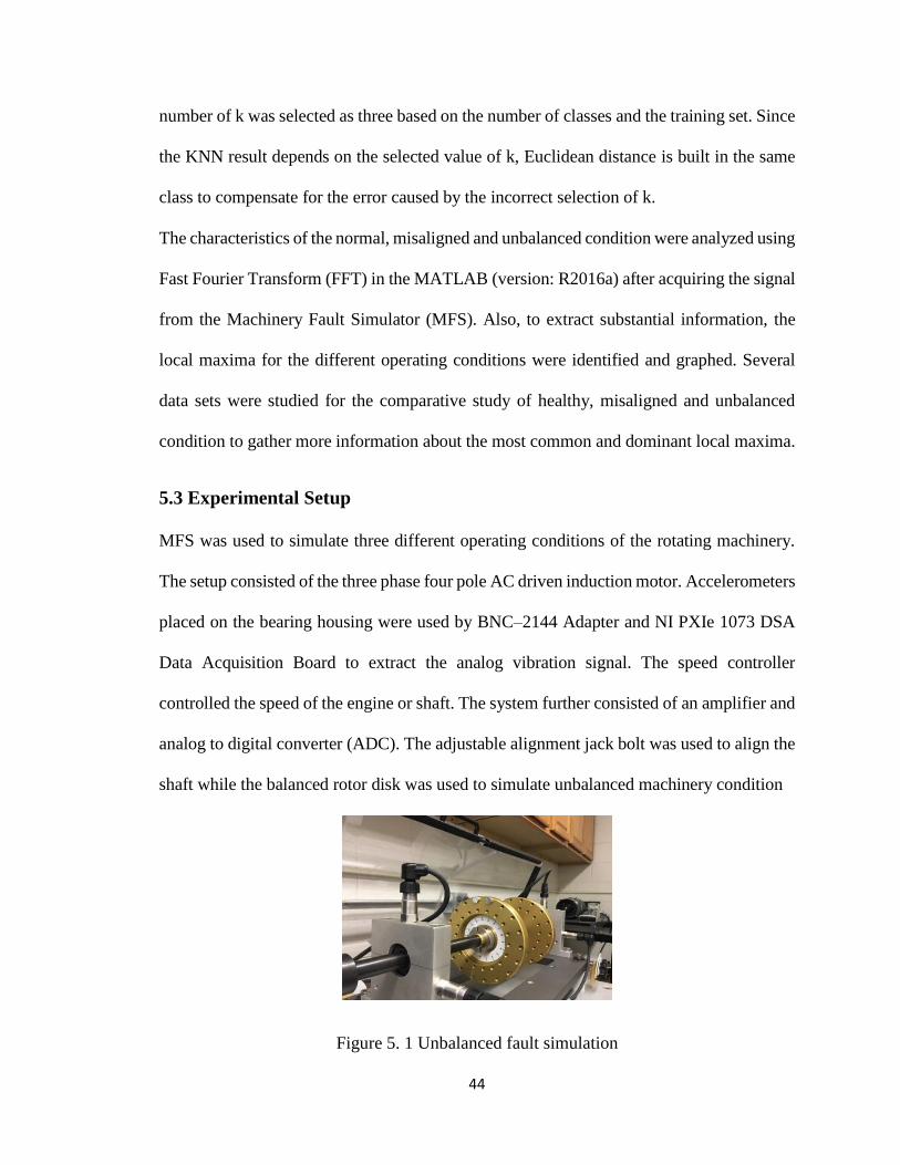
5.3 Experimental Setup

MFS was used to simulate three different operating conditions of the rotating machinery.

The setup consisted of the three phase four pole AC driven induction motor. Accelerometers

placed on the bearing housing were used by BNC–2144 Adapter and NI PXIe 1073 DSA

Data Acquisition Board to extract the analog vibration signal. The speed controller

controlled the speed of the engine or shaft. The system further consisted of an amplifier and

analog to digital converter (ADC). The adjustable alignment jack bolt was used to align the

shaft while the balanced rotor disk was used to simulate unbalanced machinery condition

Figure 5. 1 Unbalanced fault simulation

45

Figure 5. 2 Misalignment fault simulation

As illustrated in Figure 5.1 two screws of 10.2-gram were added in the threaded hole of the

left side rotor for simulating an unbalanced operating condition. Additional mass in the

form of screws was removed from the rotor disk to simulate normal operating condition.

Before extracting healthy operating condition data, the shaft was also aligned perfectly.

The system was set to operate at various motor speeds by changing the frequency to 10 Hz,

15 Hz, 20 Hz, and 25 Hz successively. The signals were extracted and further processed

using MATLAB (version: R2016a) and NI Sound and Vibration Assistant Software after

recording data. Hanning window was selected during data acquisition to minimize the

leakage in the non-periodic signal. Similarly, as shown in Figure 5.2, the alignment jack

bolt was used to misalign the shaft angularly to 10 milli inches.

5.4 Local Maxima Detection Using the Signal Analysis

As mentioned earlier, different fault conditions of machinery can be detected and predicted

using the information of energy produced at specific frequencies. Therefore, it is crucial to

have information related to frequency and energy content to monitor machinery operating

status. The spectrum acceleration curve was thus designed to study the relationship of

energy produced by the different frequencies when the system was subjected to different

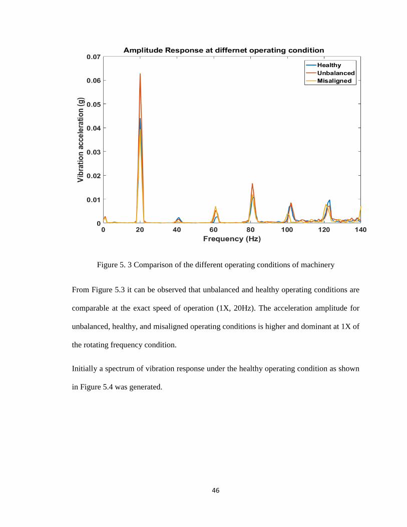
working conditions. This acceleration amplitude curve is shown in Figure 5.3.

46

Figure 5. 3 Comparison of the different operating conditions of machinery

From Figure 5.3 it can be observed that unbalanced and healthy operating conditions are

comparable at the exact speed of operation (1X, 20Hz). The acceleration amplitude for

unbalanced, healthy, and misaligned operating conditions is higher and dominant at 1X of

the rotating frequency condition.

Initially a spectrum of vibration response under the healthy operating condition as shown

in Figure 5.4 was generated.

47

Figure 5. 4 Amplitude response for healthy data

The several dominating peaks are observed from Figure 5.4. However, it is challenging to

determine the exact locations of these peaks. Then the graph was narrowed down with the

information about the first 20 harmonic speed for better visualization and analysis. The

graph contained the data of nX speed where n is the order of harmonic speed ranging from

1 to 20 while X is the system operating speed (20 Hz). The acceleration amplitude of nX

harmonic speed was plotted using the MATLAB peak finding functions which can be seen

as a red star in Figure 5.5.

It was observed that 1X is the location of the dominant peak. Other peaks appear around

harmonics of operating speed but not at them exactly. A MATLAB program was developed

to find all local maximum accelerations around 1 to 20 times operating speed. It also showed

48

that finding peaks or finding acceleration from the exact value of 1 to 20 times operating

speed can provide misleading information on the selection of functions for KNN analysis.

Figure 5. 5 Acceleration amplitude at the multi times operating speed.

A healthy operating condition analysis showed that smaller peaks are not always located at

nX speed. Since it was challenging to track the exact location of smaller peaks using the

above-discussed MATLAB graph, the program to accurately locate the first 20 local

maximum amplitude was developed. The optimum speed range had to be selected at first in

order to include the information of all the maximum local acceleration amplitude. To

compare the peaks around the harmonic speed, it was decided to select the harmonic speed

range of ±10 Hz. This program would evaluate the peaks placed between ±10 Hz from nX

harmonics. For simplicity let's say if we had to find the local maximum amplitude around

2X (where X is 20) harmonic speed, then the local peaks ranging from harmonic speed 30

49

to 50 will be compared and then the most significant peak would be identified. After

identifying the first 20 local maximum acceleration amplitudes, they were then paired with

their corresponding speed. These resulted pairs were then plotted as the blue circle in a

narrowed vibration response graph as seen in Figure 5.6.

Figure 5. 6 Local maximum acceleration amplitude plot for healthy data

As seen from the Figure the local maximum peak is taken into the account which are closer

to the harmonic speed. These local maximum acceleration amplitudes are calculated based

on the selected ranges of the acceleration between the ±10 around the periphery of the

harmonic speed. The ranges were selected based on the ability to detect all the local

maximum amplitude.

As shown in Figure 5.6 all peak amplitudes were accurately detected. Comparing the

Figures 5.5 and 5.6, it can be concluded that apart from a few peaks, most of the peaks are

not precisely at Harmonic speed.

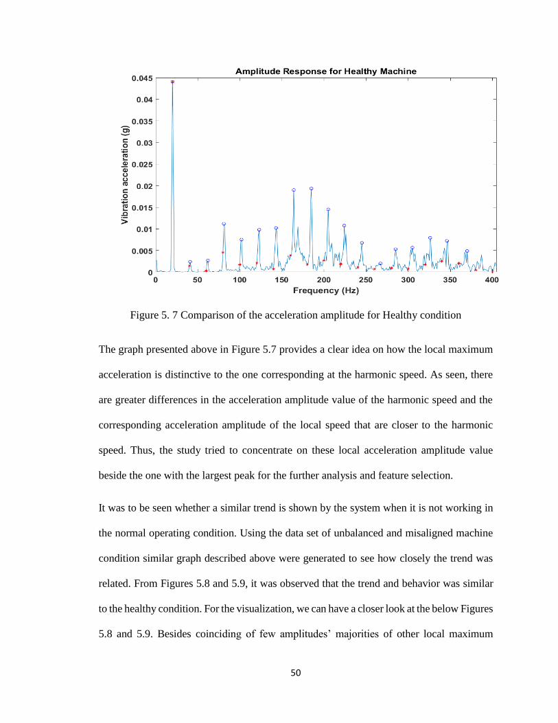
50

Figure 5. 7 Comparison of the acceleration amplitude for Healthy condition

The graph presented above in Figure 5.7 provides a clear idea on how the local maximum

acceleration is distinctive to the one corresponding at the harmonic speed. As seen, there

are greater differences in the acceleration amplitude value of the harmonic speed and the

corresponding acceleration amplitude of the local speed that are closer to the harmonic

speed. Thus, the study tried to concentrate on these local acceleration amplitude value

beside the one with the largest peak for the further analysis and feature selection.

It was to be seen whether a similar trend is shown by the system when it is not working in

the normal operating condition. Using the data set of unbalanced and misaligned machine

condition similar graph described above were generated to see how closely the trend was

related. From Figures 5.8 and 5.9, it was observed that the trend and behavior was similar

to the healthy condition. For the visualization, we can have a closer look at the below Figures

5.8 and 5.9. Besides coinciding of few amplitudes’ majorities of other local maximum

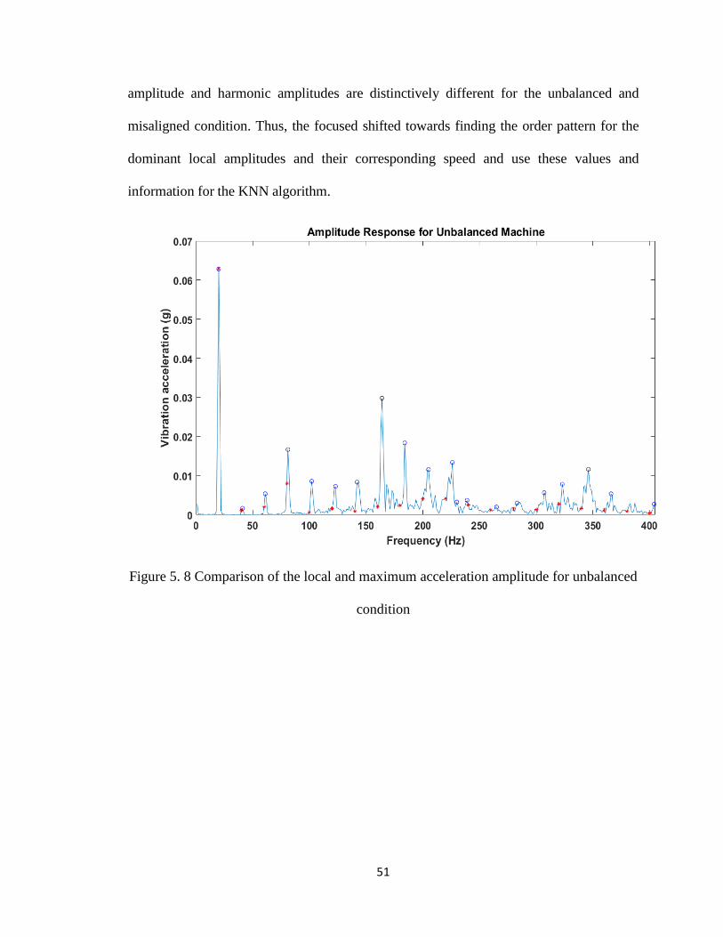
51

amplitude and harmonic amplitudes are distinctively different for the unbalanced and

misaligned condition. Thus, the focused shifted towards finding the order pattern for the

dominant local amplitudes and their corresponding speed and use these values and

information for the KNN algorithm.

Figure 5. 8 Comparison of the local and maximum acceleration amplitude for unbalanced

condition

52

Figure 5. 9 Comparison of the local and maximum acceleration amplitude for misaligned

condition

Further using other data samples, the study tried to find the dominant local maximum

acceleration amplitude and their corresponding speed.

Figure 5. 10 Comparison of the acceleration amplitude for healthy data sets.

53

It can be seen from the comparison of acceleration amplitude in Figure 5.10 for healthy

data, that besides a few amplitudes coinciding most of them are occurring at a different

speed. Using different data set of the healthy operating condition study tried to find out the

most dominating local acceleration amplitude and their corresponding speed. It was found

that the local maximum amplitude corresponding to their speed was closer to the following

harmonic speed in the descending order as 1x,9x,8x,10x,11x,4x,7x,6x ,16x.

Figure 5. 11 Comparison of the acceleration amplitude for unbalanced data sets.

Similarly, from Figure 5.11 we can see that there are differences in the amplitude

acceleration and local maximum one besides a few coinciding amplitudes. These

Unbalanced operating condition data set showed that the maximum amplitude is not always

occurring at multi times of operating speed. Looking at the pattern, the descending order

54

of the local maximum amplitude closer to the harmonic speed were as 1x, 8x,9x, 10x,

16x.11x,4x,6x.

Figure 5. 12 Comparison of the acceleration amplitude for misaligned data sets.

The pattern was like one of Healthy and Unbalanced data set for the misaligned operating

condition. The dominating local maximum amplitude closer to the harmonic speed were as

1x,8x,11x,9x,16x,10x,4x.

After the analysis first six common dominant order for all three-operating condition

of the machinery were found as 1x, 8x, 9x, 11x, 16x, and 10x RPM. Therefore, the above

six dominant orders were selected as six features for KNN algorithm features

5.5 Results

The features based on the order of the dominant local maximum acceleration amplitude

were further studied to see the most significant one. 1x RPM and 16x RPM were found to

be the most significant features when compared to the 95% confidence interval using

55

Tukey's method. The selected features were then used to generate training data for the

proposed KNN classifier. Euclidean distance function was used as a distance metric for the

classifier. Using the training data set the Euclidean distance of the testing data sets were

calculated. The number of nearest neighbor K was chosen as 3. The classes closer to the

minimum distance were ranked in ascending order after calculating the Euclidean distance.

The test data set class label is then classified based on its closest neighbor's majority class.

The model was tested using the unknown operating condition data set where it

demonstrated excellent fault classification capabilities. It showed satisfactory accuracy of

over 96%. Since the proposed method concentrate on identifying the local dominant peaks

and its corresponding harmonic speed rather than concentrating on just harmonic amplitude

and its corresponding speed, the identification, and classification of the different operating

condition becomes more efficient. Tables 5.1 and 5.2 show the result of the classification

for the proposed KNN method.

56

Table 5. 1 Unknown Testing Data Sets

Testing

Dataset

Feature1

1x RPM

Feature2

8x RPM

Feature3

9x RPM

Feature4

11x RPM

Feature5

10x RPM

Feature6

16x RPM

Situation

1 0.045027 0.021722 0.01227 0.009155 0.013987 0.009374 Unknown

2 0.043975 0.008434 0.024332 0.007996 0.010282 0.009226 Unknown

3 0.044651 0.022586 0.010738 0.01473 0.01525 0.008634 Unknown

4 0.063556 0.042059 0.020411 0.009278 0.008583 0.00876 Unknown

5 0.063247 0.028454 0.012991 0.019314 0.012181 0.004144 Unknown

6 0.063155 0.01924 0.018068 0.011175 0.008922 0.007019 Unknown

7 0.039874 0.016669 0.011933 0.025645 0.010187 0.009802 Unknown

8 0.040065 0.01151 0.012123 0.010416 0.008755 0.009174 Unknown

9 0.040579 0.013342 0.0142 0.01036 0.007299 0.013818 Unknown

57

Table 5. 2 KNN Fault Classification Based on the Local Harmonic Amplitude

Feature1

1x RPM

Feature2

8x RPM

Feature3

9x RPM

Feature4

11x RPM

Feature5

10x RPM

Feature6

16x RPM

Rank Euclidean

Distance

Category

0.044069 0.019011 0.019337 0.010756 0.014503 0.007936 5 0.004867133 Healthy

0.046403 0.016859 0.023506 0.008721 0.016715 0.006386 12 0.006984217 Healthy

0.046179 0.019703 0.018243 0.011807 0.019856 0.006263 11 0.006436746 Healthy

0.044328 0.026735 0.017797 0.011218 0.018571 0.007009 8 0.005336826 Healthy

0.043794 0.027905 0.017037 0.01423 0.009442 0.008671 4 0.004168619 Healthy

0.045027 0.02629 0.0215 0.014755 0.007172 0.006369 10 0.006261113 Healthy

0.062562 0.04247 0.016599 0.017554 0.020773 0.011169 13 0.014872686 Unbalanced

0.062815 0.029798 0.018373 0.01336 0.011563 0.00782 14 0.015505756 Unbalanced

0.063347 0.031236 0.016461 0.00731 0.019909 0.008812 15 0.015654394 Unbalanced

0.063189 0.039176 0.017107 0.021397 0.010365 0.006347 16 0.016000239 Unbalanced

0.063668 0.029883 0.019234 0.020621 0.015014 0.004562 18 0.01676255 Unbalanced

0.063265 0.031205 0.019234 0.016034 0.020179 0.005897 17 0.016197614 Unbalanced

0.039384 0.019155 0.012509 0.018313 0.007255 0.007836 3 0.004126924 Misaligned

0.039585 0.027924 0.01551 0.016732 0.007296 0.01142 2 0.001789946 Misaligned

0.039598 0.020953 0.018866 0.02686 0.011592 0.006948 6 0.004883526 Misaligned

0.040194 0.015063 0.007774 0.01763 0.007633 0.006339 9 0.005419133 Misaligned

0.039581 0.006451 0.013812 0.013578 0.006263 0.01396 1 0.000687263 Misaligned

0.040428 0.018695 0.015676 0.014285 0.006702 0.00593 7 0.005312943 Misaligned

58

Table 5. 3 Testing Data with the unknown operating condition

Feature1

1x RPM

Feature2

8x RPM

Feature3

9x RPM

Feature4

11x RPM

Feature5

10x RPM

Feature6

16x RPM

0.040579 0.013342 0.0142 0.01036 0.007299 0.013818

Table 5. 4 Result of the KNN testing

Test Data K=1 K=2 K=3

1 Misaligned Misaligned Misaligned

Result: Machine is operating in Misaligned condition

As can be seen from the above table, this method showed good fault classification

capabilities. This method can be used for the classification of the fault in the industries for

better accuracy and predictability.

Chapter Summary

Even though the first order frequency shows peak amplitude it is not always the case with

the other remaining order to have similar peaks, the other smaller peaks usually does not

always occur at the multi times operating frequency instead they occur at the frequency

closer to these frequencies. These maximum peaks were referred as the local maximum.

By focusing on the local maximum acceleration amplitude rather than amplitude at the

harmonic speed a KNN based algorithm was developed which could classify the operating

59

status of the rotating machinery correctly using the features of the local maximum

acceleration around the harmonic speed.

60

Chapter VI

6. Conclusion and Future Work

6.1 Conclusion

Industries deploying rotating machinery aim to operate them smoothly so that their revenue

generation is not hampered. It can be said that these industries look for safe, reliable and

cost efficient operation to match their organizational goals. Efficient monitoring of these

machinery with a reliable diagnostic tool can ensure industries to meet their above

mentioned desirability. Vibration analysis is one of the most popular conditions monitoring

approach used in modern day industries, it uses vibration signal to monitor the operating

condition of the machinery. Since these are signal based monitoring approach, there need

to be an adequate understanding of the signal for efficient monitoring. One should have a

better understanding of utilizing the time and frequency related information to detect and

identify different machine fault. On the other hand, one should have familiarity with the

complexity of vibration analysis for these industries need an expert or professional analyst

to carry out vibration analysis. So the industries are looking for the cost-effective, easily

interpretable and efficient vibration monitoring tool. Most of the time, focus has been laid

on the time domain signal to detect the fault while frequency domain information is used

for identifying the fault type. Similarly, the multi times operating speed’s amplitude is

considered for developing a vibration-based condition monitoring tool. The aim of this

research project is to develop efficient, economical, and straightforward monitoring tools

that could utilize time domain signal to identify not only the fault but also classify the fault

type. Similarly, the local maximum acceleration-based fault detection is proposed further.

61

The vibration signal of the machinery system is extracted by simulating it to different

operating condition as healthy, misaligned, unbalanced and cracked shaft. Once these data

are acquired they are processed using the signal processing tool like FFT and CWT for

understanding the characteristic features of each operating condition, once these are known

fault classification and detection tool are developed. Phase plane diagram-based tool

utilizes the signal from all the 4 accelerometers to classify the fault while the KNN method

based on the local maximum acceleration uses the frequency information for classifying

the fault. Similarly, fuzzy logic based method is proposed for classifying the fault and

identifying the severity of machine condition. The proposed method showed greater

accuracy and efficiency in identifying and classifying the machine condition. So they can

be implemented in the industries for the monitoring purpose.

6.2 Future Work

The proposed methodology can be incorporated with Artificial Intelligence System for not

only detecting and classifying fault but also diagnosing or correcting it. This work also

forms a solid basis for stability analysis in rotating machinery using CAD/CAE based

approach. Thus, it is important to investigate on how stiffness and damping coefficients

affect rotor systems. Various numerical methods can be used for such analysis and a simple

fuzzy based system could be developed to validate the results. Furthermore, for the

reliability of the proposed methods, data will be acquired in real environmental conditions

from operating machines with larger sample size instead simulating in a laboratory setting.

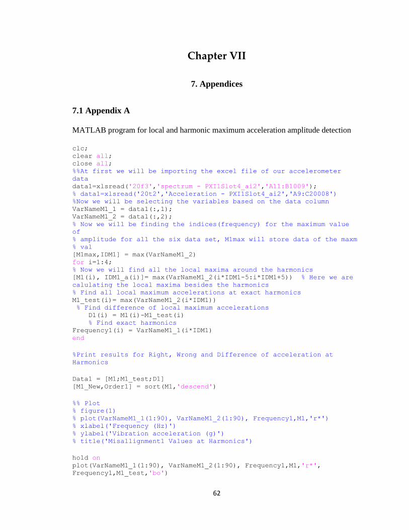
62

Chapter VII

7. Appendices

7.1 Appendix A

MATLAB program for local and harmonic maximum acceleration amplitude detection

clc; clear all; close all; %%At first we will be importing the excel file of our accelerometer

data data1=xlsread('20f3','spectrum - PXI1Slot4_ai2','A11:B1009'); % data1=xlsread('20t2','Acceleration - PXI1Slot4_ai2','A9:C20008') %Now we will be selecting the variables based on the data column VarNameM1_1 = data1(:,1); VarNameM1_2 = data1(:,2); % Now we will be finding the indices(frequency) for the maximum value

of % amplitude for all the six data set, M1max will store data of the maxm % val [M1max,IDM1] = max(VarNameM1_2) for i=1:4; % Now we will find all the local maxima around the harmonics [M1(i), IDM1_a(i)]= max(VarNameM1_2(i*IDM1-5:i*IDM1+5)) % Here we are

calulating the local maxima besides the harmonics % Find all local maximum accelerations at exact harmonics M1_test(i)= max(VarNameM1_2(i*IDM1)) % Find difference of local maximum accelerations D1(i) = M1(i)-M1_test(i) % Find exact harmonics Frequency1(i) = VarNameM1_1(i*IDM1) end

%Print results for Right, Wrong and Difference of acceleration at

Harmonics

Data1 = [M1;M1_test;D1] [M1_New,Order1] = sort(M1,'descend')

%% Plot % figure(1) % plot(VarNameM1_1(1:90), VarNameM1_2(1:90), Frequency1,M1,'r*') % xlabel('Frequency (Hz)') % ylabel('Vibration acceleration (g)') % title('Misallignment1 Values at Harmonics')

hold on plot(VarNameM1_1(1:90), VarNameM1_2(1:90), Frequency1,M1,'r*',

Frequency1,M1_test,'bo')

63

xlabel('Frequency (Hz)') ylabel('Vibration acceleration (g)') title('Misallignment1 Values at Harmonics')

64

References

[1] S. Rao, Mechanical Vibration, 5th ed., NJ Pearson Education Inc., 2010.

[2] B. K. N. Rao, Handbook of condition monitoring, Elsevier, 1996.

[3] P. J. Tavner, J. Penman, Condition Monitoring of Electrical Machines, U.K., Letchworth:Res.

Studies Press, 1987.

[4] A. Brandt, Noise and Vibration Analysis: Signal Analysis and Experimental Procedures, 2011.

[5] R. K. Mobley, An Introduction to Predictive Maintenance (Second Edition), 2002.

[6] P. Tavner, "Review of condition monitoring of rotating electrical machines," IET Electric

Power Applications, vol. 2, no. 4, pp. 215-247, 2008.

[7] E. Kannatey-Asibu and D. A. Dornfeld, "Quantitative Relationships for Acoustic Emission

from Orthogonal Metal Cutting," Journal of Engineering for Industry, vol. 103, no. 3, pp. 330-

340, 1981.

[8] E. Kannatey-Asibu and E. Emel, "Linear discriminant function analysis of acoustic emission

signals for cutting tool monitoring," Mechanical Systems and Signal Processing, vol. 1, no. 4,

pp. 333-347, 1 10 1987.

[9] D. Dornfeld, "Application of acoustic emission techniques in manufacturing," NDT and E

International, vol. 25, no. 6, pp. 259-269, 1992.

[10] . Bagavathiappan, B. B. Lahiri, T. Saravanan, J. Philip and T. Jayakumar, "Infrared

thermography for condition monitoring - A review," Infrared Physics and Technology, vol.

60, pp. 35-55, 2013.

[11] R. K. Will, E. F. Ring, A. K. Clarke and P. J. Maddison, "Infrared thermography: What is its

place in rheumatology in the 1990s?," Rheumatology, vol. 31, no. 5, pp. 337-344, 1992.

[12] O. Janssens, R. Schulz, V. Slavkovikj, K. Stockman, M. Loccufier, R. Van De Walle and S. Van

Hoecke, "Thermal image based fault diagnosis for rotating machinery," Infrared Physics and

Technology, vol. 73, pp. 78-87, 2015.

[13] K. M. Reichard, M. Van Dyke and K. Maynard, "Application of sensor fusion and signal

classification techniques in a distributed machinery condition monitoring system," Sensor

Fusion: Architectures, Algorithms, and Applications IV, vol. 4051, pp. 329-336, 2000.

[14] M. P. Luong, "Fatigue limit evaluation of metals using an infrared thermographic technique,"

Mechanics of Materials, vol. 28, no. 1-4, pp. 155-163, 1998.

65

[15] F. Curà, G. Curti, Sesana. R. and R. Sesana, "A new iteration method for the thermographic

determination of fatigue limit in steels," International Journal of Fatigue, vol. 27, no. 4, pp.

453-459, 2005.

[16] G.-M. Lim, D.-M. Bae and J.-H. Kim, "Fault diagnosis of rotating machine by thermography

method on support vector machine," Journal of Mechanical Science and Technology, vol. 28,

no. 8, pp. 2947-2952, 15 8 2014.

[17] S. JS, "Failure Prediction Using Ferrographic Oil Analysis Techniques," in Conference on

lubrication, friction and wear in engineering, 1980 : Melbourne 1-5 December 1980 :

preprints of papers, 1980.

[18] I. M. Flanagan, J. R. Jordan, H. W. Whittington -Wear and D. Scott -Recent, "Wear-debris

detection and analysis techniques for lubricant-based condition monitoring," Journal of

Physics E: Scientific Instruments, vol. 21, p. 11, 1988.

[19] T. H. Loutas, D. Roulias, E. Pauly and V. Kostopoulos, "The combined use of vibration,

acoustic emission and oil debris on-line monitoring towards a more effective condition

monitoring of rotating machinery," Mechanical Systems and Signal Processing, vol. 25, no.

4, pp. 1339-1352, 2011.

[20] S. Poyhonen, P. Jover and H. Hyotyniemi, "Signal processing of vibrations for condition

monitoring of an induction motor," in First International Symposium on Control,

Communications and Signal Processing, pp. 499-502.

[21] A. Lachouri, K. Baiche, R. Djeghader, N. Doghmane and S. Oulitati, "Analyze and fault

diagnosis by multi-scale PCA," in 2008 3rd International Conference on Information and

Communication Technologies: From Theory to Applications, ICTTA, 2008, pp. 1-6.

[22] L. Jiang, Z. Liu, J. Cui and Z. Li, "Condition monitoring of rolling element bearing based on

Phase-PCA," in 2013 25th Chinese Control and Decision Conference (CCDC), 2013, pp. 1082-

1086.

[23] C. Harlisca, L. Szabo, L. Frosini and A. Albini, "Bearing faults detection in induction machines

based on statistical processing of the stray fluxes measurements," in Proceedings - 2013 9th

IEEE International Symposium on Diagnostics for Electric Machines, Power Electronics and

Drives, SDEMPED 2013, 2013, pp. 371-376.

[24] C.-z. Hu, M.-y. Huang, Q. Yang and W.-j. Yan, "On the use of EEMD and SVM based approach

for bearing fault diagnosis of wind turbine gearbox," in 2016 Chinese Control and Decision

Conference (CCDC), 2016, pp. 3472-3477.

[25] Na Li, Mei-cheng Chen, Yan-jun Fang and Hong Li, "Fault Diagnose of Rotating System Based

on ICA with Reference and RBF Networks," in 2006 IEEE International Conference on

Networking, Sensing and Control, pp. 174-178.

66

[26] R. B. Randall, Vibration-Based Condition Monitoring: Industrial, Aerospace and Automotive

Applications, John Wiley & Sons, 2011.

[27] D. Dyer and R. M. Stewart, "Detection of Rolling Element Bearing Damage by Statistical

Vibration Analysis," Journal of Mechanical Design, vol. 100, no. 2, p. 229, 1 4 1978.

[28] P. D. Mcfadden and J. D. Smith, "A signal processing technique for detecting local defects in

a gear from the signal average of the vibration," Proceedings of the Institution of Mechanical

Engineers, Part C: Journal of Mechanical Engineering Science, vol. 199, no. 4, pp. 287-292,

1985.

[29] M. Xu and R. D. Marangoni, "Vibration analysis of a motor-flexible coupling-rotor system

subject to misalignment and unbalance, Part I: Theoretical model and analysis," Journal of

Sound and Vibration, vol. 176, no. 5, pp. 663-679, 1994.

[30] P. Domingos, "A few useful things to know about machine learning," Communications of the

ACM, 2012.

[31] B. Samanta, "Gear fault detection using artificial neural networks and support vector

machines with genetic algorithms," Mechanical Systems and Signal Processing, vol. 18, no.

3, pp. 625-644, 2004.

[32] F. Jia, Y. Lei, J. Lin, X. Zhou and N. Lu, "Deep neural networks: A promising tool for fault

characteristic mining and intelligent diagnosis of rotating machinery with massive data,"

Mechanical Systems and Signal Processing, vol. 72, pp. 303-315, 2016.

[33] S. Goldman, Vibration spectrum analysis: a practical approach., Industrial Press Inc, 1999.

[34] A. K. Jardine, D. Lin and D. Banjevic, "A review on machinery diagnostics and prognostics

implementing condition-based maintenance," Mechanical Systems and Signal Processing,

vol. 20, no. 7, pp. 1483-1510, 2006.

[35] Y. M. Zhan and A. K. Jardine, "Adaptive autoregressive modeling of non-stationary vibration

signals under distinct gear states. Part 1: Modeling," Journal of Sound and Vibration, vol.

286, no. 3, pp. 429-450, 2005.

[36] L. Cohen, Time-frequency analysis, Volume 778 ed., Prentice Hall PTR Englewood Cliffs,

1995.

[37] W. J. Staszewski, K. Worden and G. R. Tomlinson, "Time-frequency analysis in gearbox fault

detection using the Wigner-Ville distribution and pattern recognition," Mechanical Systems

and Signal Processing, vol. 11, no. 5, pp. 673-692, 1997.

[38] N. Baydar and A. Ball, "A comparative study of acoustic and vibration signals in detection of

gear failures using Wigner-Ville distribution," Mechanical Systems and Signal Processing,

vol. 15, no. 6, pp. 1091-1107, 2001.

67

[39] W. J. Staszewski, "Wavelet based compression and feature selection for vibration analysis,"

Journal of Sound and Vibration, vol. 211, no. 5, pp. 735-760, 1998.

[40] W. J. Wang and P. D. McFadden, "Application of wavelets to gear box vibration signals for

fault detection," Journal of Sound and Vibration, vol. 192, no. 5, pp. 927-39, 1996.

[41] G. Y. Luo, D. Osypiw and M. Irle, "On-line vibration analysis with fast continuous wavelet

algorithm for condition monitoring of bearing," JVC/Journal of Vibration and Control, vol. 9,

no. 8, pp. 931-947, 2003.

[42] Harder Douglas, "Mathematical Introduction to Fuzzy Logic, Fuzzy Sets, and Fuzzy Controls,"

2004.[Online].

Available: https://www.maplesoft.com/applications/view.aspx?SID=1409&view=html.

[43] Mathworks Inc., MATLAB and statistics toolbox release, 2016.

[44] S. Nandi, H. A. Toliyat and X. Li, "Condition monitoring and fault diagnosis of electrical

motors - A review," IEEE Transactions on Energy Conversion, vol. 20, no. 4, pp. 719-729,

2005.

[45] A. K. Jalan and A. R. Mohanty, "Model based fault diagnosis of a rotor-bearing system for

misalignment and unbalance under steady-state condition," Journal of Sound and Vibration,

vol. 327, no. 3-5, pp. 604-622, 2009.

[46] T. Plante, A. Nejadpak and C. X. Yang, "Faults detection and failures prediction using

vibration analysis," in AUTOTESTCON (Proceedings), 2015, pp. 227-231.

[47] E. Alpaydin, Introduction to machine learning Ethem Alpaydin., 2014.

[48] P. Lison, "An introduction to machine learning", "" Language Technology Group (LTG), 1-35

,2015.

[49] B. A. Paya, I. I. Esat and M. N. Badi, "Artificial neural network based fault diagnostics of

rotating machinery using wavelet transforms as a preprocessor," Mechanical Systems and

Signal Processing, vol. 11, no. 5, pp. 751-765, 1997.

[50] L. B. Jack and A. K. Nandi, "Fault detection using support vector machines and artificial

neural networks, augmented by genetic algorithms," Mechanical Systems and Signal

Processing, vol. 16, no. 2-3, pp. 373-390, 2002.

[51] D. H. Pandya, S. H. Upadhyay and S. P. Harsha, "Fault diagnosis of rolling element bearing

with intrinsic mode function of acoustic emission data using APF-KNN," Expert Systems with

Applications, vol. 40, no. 10, pp. 4137-4145, 2013.

68

[52] Y. Lei and M. J. Zuo, "Gear crack level identification based on weighted K nearest neighbor

classification algorithm," Mechanical Systems and Signal Processing, vol. 23, no. 5, pp. 1535-

1547, 2009.

[53] A. Nejadpak and C. X. Yang, "Misalignment and Unbalance Faults Detection and

Identification Using KNN Analysis," in Proceedings of CANCAM 2017, 2017, pp. 1–4.

[54] T. M. Cover and P. E. Hart, "Nearest Neighbor Pattern Classification," IEEE Transactions on

Information Theory, vol. 13, no. 1, pp. 21-27, 1967.

[55] C. Li, S. Zhang, H. Zhang, L. Pang, K. Lam, C. Hui and S. Zhang, "Using the K-nearest neighbor

algorithm for the classification of lymph node metastasis in gastric cancer.," Computational

and mathematical methods in medicine, pp. 1-11, 2012.