Vibration Theory, Vol. 1B linear vibration theory, MATLAB ...

Aalborg Universitet

Vibration Theory, Vol. 1B

linear vibration theory, MATLAB exercises

Asmussen, J. C.; Nielsen, Søren R. K.

Publication date:1996

Document VersionPublisher's PDF, also known as Version of record

Link to publication from Aalborg University

Citation for published version (APA):Asmussen, J. C., & Nielsen, S. R. K. (1996). Vibration Theory, Vol. 1B: linear vibration theory, MATLABexercises. Department of Mechanical Engineering, Aalborg University. U/ No. 9601

General rightsCopyright and moral rights for the publications made accessible in the public portal are retained by the authors and/or other copyright ownersand it is a condition of accessing publications that users recognise and abide by the legal requirements associated with these rights.

- Users may download and print one copy of any publication from the public portal for the purpose of private study or research. - You may not further distribute the material or use it for any profit-making activity or commercial gain - You may freely distribute the URL identifying the publication in the public portal -

Take down policyIf you believe that this document breaches copyright please contact us at [email protected] providing details, and we will remove access tothe work immediately and investigate your claim.

Downloaded from vbn.aau.dk on: July 13, 2022

https://vbn.aau.dk/en/publications/0b993280-a86a-11da-8341-000ea68e967b

VIBRATION THEORY, VOL. lB

Linear Vibration Theory MATLAB Exercises

John C . Asmussen S!Ziren R.K. Nielsen

Aalborg tekniske Universitetsforlag February, 1996

VIBRATION THEORY, VOL. lB

Linear Vibration Theory MATLAB Exercises

John C. Asmussen S~ren R.K. Nielsen

Aalborg tekniske Universitetsforlag February, 1996

PREFACE

The present collection of MATLAB exercises has been published as a supplement to the textbook, Svingningsteori, Bind 1 and the collection of exercises in Vibration theory, Vol. 1 A, Solved Problems. Throughout the exercises references are made to these books.

The purpose of the MATLAB exercises is to give a better understanding of the physical problems in linear vibration theory and to suppress the mathematical analysis used to solve the problems. For this purpose the MATLAB environment is excellent.

It is possible to get help to every file by typing help exerc?? or .help plot??, where ?? denotes the number of the exercises. All m-files will be available on a discette.

University of Aalborg, February, 1996 S!llren R.K. Nielsen John C. Asmussen

Contents

1 Lecture 1 3 1.1 MATLAB Exercise 1 3

1.1.1 MATLAB Solution 0 3 1.1.2 MATLAB Files 0 0 0 4

1.2 MATLAB Exercise 2 0 0 0 0 5 1.201 MATLAB Solution 0 5 1.202 MATLAB Files 0 0 0 6

2 Lecture 2 8 201 MATLAB Exercise 3 8

201.1 MATLAB Solution 0 8 201.2 MATLAB Files 0 0 0 11

3 Lecture 3 14

3°1 MATLAB Exercise 4 14 301.1 MATLAB Solution 0 15 301.2 MATLAB Files 0 0 0 18



402 MATLAB Exercise 6 0 0 0 0 25 40201 MATLAB Solution 0 26 40202 MATLAB Files 0 29


5 01.1 MATLAB Solution 0 33 501.2 MATLAB Files 0 0 0 34


601.1 0 MATLAB Solution 37 601.2 MATLAB Files 0 0 39



1

2

8 Lecture 8 8 .1 MATLAB Exercise 10

8.1.1 MATLAB Solution . 8.1.2 MATLAB Files ...

9 Lecture 9 9.1 MATLAB Exercise 11

9.1.1 MATLAB Solution . 9.1.2 MATLAB Files .


10.1.1 MATLAB Solution . 10.1.2 MATLAB Files .


11.1.1 MATLAB Solution . 11 .1.2 MATLAB Files .. .

A Lecture 4

CONTENTS

50 50 50 52

55 55 56 56

58 58 59 64

65 65 66 69

70

Chapter 1

Lecture 1

Problem 1 and 4 of lecture 1 are solved theoretically. The solutions to these problems can be found in Nielsen [2]. The following MATLAB exercises replaces the corresponding problem 2 and 3.

1.1 MATLAB Exercise 1

The Fourier series of problem 1, lecture 1 1s considered and the following truncated series 1s considered.

{1.1)

Plot the function Xn(t) as a function of time fort E ] - 47r, 47r[ and n = 3, 10, 30. Compare the different Fourier series with the sawtooth function graphically.

1.1.1 MATLAB Solution

The MATLAB functions below (exercl .m , plotl.m) shows how MATLAB exercise 1, lecture 1 could be solved. If the following four orders are given:

{xi , t}=exercl (1 000,3}; {x2, t}=exercl (1 000,1 0}; [x3, t}=exercl (1000,30); plotl (t ,xl,x2,x3};

Then figure 1.1 will appear on the screen. An explanation of the input numbers can be found in the head of the MATLAB functions (exercl.m, plotl.m).

3

4 CHAPTER 1. LECTURE 1

~ltl-----.-z~4Z~4!-----,L-~-4---,l.-?~! -1~5----------1~0~--------~5---------~0--------~5--------1~0 ________ _j15

~·~lf--T----v~4----r--L1v~1~v~------l-.-.lj -1~5----L-----1~0------~--~5--------~0--------~5--L------1~0--------_J15

Time [s]

Figure 1.1: Sawtooth approximations between J - 47r, 47r[, as a function of the number of harmonics,

n. a) n=3, b) n=10, c) n=30.

1.1.2 MATLAB Files ****************************************************************

MATLAB Function Purpose

File for MATLAB Exercise 1, Lecture 1 EXERC1.M To calculate the Fourier series from Exercise 1, Lecture 1.

Call exercl {n,no) n Number of iliscrete time points b etween -4*pi and 4*pi. no Number of summations in Fourier series Return (Fx,t) Xno Vector with sum of Fourier series t Vector with time components

**************************************************************** function [Xno,t)= exercl{n,no); dt=( 4*pi+4*pi)/(n-1}; t=-4 *pi :dt :4 *pi; for l=1:n, Xno(l)=O; for m=-no:no, if (m==O) Am=0.5; else Am=i/{2*m*pi); end; Xno(l)=Am*exp{i*m*t(l))+Xno{l); end; end; ****************************************************************

1.2. MATLAB EXERCISE 2

**************************************************************** MATLAB Function Purpose

Call

x1 x2 x3 Return

File for MATLAB Exercise 1, Lecture 1 PLOTl .M To plot the sawtooth approximations from the Fourier series in Problem 1, Lecture 1 plotl ( t,x1,x2,x3) Time vector First sawtooth approximation Second s awtooth approximation Third sawtooth approximation Graphical plot of approximations

**************************************************************** function plotl(t,xl,x2,x3); xl=real(x1); x2=real(x2); x3=real(x3); tt(1)=-15; tt(2)=15; xx(1)=0.5; xx(2)=0.5; tt1(1)=-2*pi; tt1(2)=-2*pi; xx1(1)=1; xx1(2)=0; tt2(1)=0; tt2(2)=0; xx2(1)=1; xx2(2)=0; tt3(1)=2*pi; tt3(2)=2*pi; xx3(1)=1; xx3(2)=0; clg; subplot(3,1 ,1) ,plot(t,x1 , tt,xx,tt 1,xx1 ,tt2,xx2,tt3,xx3); ylabel('a) 1. Approx.'); axis((-15 15 -0.11.1]); subplot(3,1,2) ,plot(t,x2,tt,xx,ttl ,xx1 ,tt2,xx2,tt3,xx3); ylabel('b) 2. Approx.'); axis((-15 15 -0.1 1.1]); subplot(3, 1 ,3) ,plot ( t,x3, tt,xx, t t 1 ,xxl ,tt2 ,xx2 ,tt3,xx3) ; ylabel('c) 3 . Approx.'); xlabel( 'Time (s] '); axis([-15 15 -0 .1 1.1]) ; ****************************************************************


The system of problem 4, lecture 1 is considered. Let the initial conditions of the system be given as follows:

a . 2 a xo = - -wo 100

(1.2) xo = 100

Plot the displacement response x(t) , and the velocity response, x(t) , as a function of time in the interval t E [0, T] . On the plot the displacement response is made non-dimensional with respect to x0 , and the velocity response is made non-dimensional with respect to jx0 j. Use the following data:

l = lm, a= 0.3m, S = 1kN, m= 0.5kg, 2.0kg (1.3)

Compare the responses with respect to the different eigenfrequencies graphically (the time periods should be equal). This should be done by comparing the two different time-displacement graphs and the two different time-velocity graphs.


The MATLAB functions below (exerc2.m, plot2.m) shows how MATLAB exercise · 2, lecture 1 could be solved. If the following three orders are given:

{x1, dx1, t]=exerc2(1, 0.3,1, 0.5,1 000, 0. 01 , 0. 009,-0.006); {x2, dx2, t]=exerc2(1, 0.3,1, 2. 0,1000, 0. 01, 0. 003,-0. 006); plot2(t,x1,x2, dx1, dx2};

5


Then figure 1.2 will appear on the screen . An explanation of the input numbers can be found in the head of the MATLAB functions (exerc2.m, plot2.m). Compare the two different timedisplacement graphs and the two different time-velocity graphs.

~·~ E ~ 2

~ 0

~-2 "-

40 I 2 3 4 5 6 7 8 9 I 0

'E4~ ~ 2 .

!-~ .o-4

0 I 2 3 4 5 6 7 8 9 10

HZSZVSZ\Zj ,. -2{j I 2 3 4 5 6 7 8 9 10

nzs;;~ .o-2{j I 2 3 4 5 6 7 8 9 10

Time [s)

Figure 1.2: Displacement and velocity responses for a) m=0.5kg and b) m=2.0kg.

1.2.2 MATLAB Files

MAT LAB Function Purpose

Call 1 a s m n dt xO dxO Return X

dx

File for MATLAB Excercise 2, Lecture 1 EXERC2.M To calculate the displacement response and the velocity resp onse of the system described in Problem 4, Lecture 1 exerc2(l,a,S,m,n,dt,x0,dx0) (see fig. Problem 4) Length of stucture Distance to mass Tension Force Mass Number of points in discrete time Time difference between points Initial displacement Initial velocity/ eigenfrequency (x,dx,t) Displacement response vector Velocity response vector Time vector

************************************************************** function (x,dx,t]=exerc2(l ,a,S,m,n,dt ,xO,dxO) omO=sqrt(l*S/ (m*a*{l-a))) ; dxO=dxO*omO; for i=l :n, t{i)=(i-l)*dt; x(i )=xO*cos( omO*t(i) )+dxO*sin( omO*t(i) )/ omO; dx(i)=-xO*ornO*sin( omO*t(i) )+dxO*cos( ornO*t(i)) ;


end; x=x/xO; dx= dx / sqrt ( dx0"2); **************************************************************

************************************************************** MATLAB Function Purpose

Call

x1 x2 dxl dx2 Return

File for MATLAB Exercise 2, Lecture 1 PLOT2.M To plot the displacement response and the velocity response in Problem 4, Lecture 1 plot2 ( t,x1 ,x2 ,dxl ,dx2) Time vector Displacement (1. eigenfrequency) Displacement (2. eigenfrequency) Velocity (1. eigenfrequency) Velocity (2. eigenfrequency) Graphical plot

************************************************************** function plot2(t ,x1,x2,dx1,dx2) clg; subplot( 4,1 ,1 ) ,plot(t ,x1); ylabel( 'a) Disp. [m]'); subplot ( 4,1 ,2) ,plot(t,x2); ylabel('b) Disp. [m]'); subplot( 4,1 ,3),plot(t ,dxl) ; ylabel( 'a) Vel. [m/s]'); subplot( 4,1 ,4) ,plot(t ,dx2) ; xlabel( 'Time [s] '); ylabel( 'b) Vel. [m/s]'); **************************************************************

7

Chapter 2

Lecture 2

Problem 1 and 3 of lecture 2 are solved theoretically. The solutions ·of these problems can be found in Nielsen (2]. The following MATLAB exercise 3 replaces the corresponding problem 2, lecture 2.


The iriitial condition of the system in problem 3, lecture 2, is defined by the clock-wise rotation from the statical equilibrium state </J.

7r

<Po = 24 . 7r

<Po = 12

wo (2.1)

Plot the vertical displacement x(t) and the velocity x(t) of the beam at the position of the linear spring, k, as a function of the non-dimensional time io, where To = ~ is the fundamental eigenperiod. Use the following data:

b = 1m, m= lkg, kg

c = 127r, 611", 0.611"s

(2 .2)

For critical damping plot the vertical displacement x(t) and the vertical velocity x(t) for a positive initial velocity, zero initial velocity and negative initial velocity.


The MATLAB functions below (exerc3.m , plot3a.m) shows how MATLAB exercise 3, lecture 2 could be solved. An explanation of the input numbers can be found in the head of the MATLAB functions (exerc3.m, plot3a.m). If the following four orders are given:

{xl, dxl , t]=exerc3(1,2/3,4 *pt 2, 1, 12*pi, 1000,0. 0025,pi/24,pi/12}; [x2, dx2, t}=exerc3(1,2/3,4 *piA 2, 1, 6*pi, 1000,0. 0025,pi/24,pi/12); [x3, dx3, t]=exerc3(1, 2/3,4*pt 2, 1, 0. 6*pi, 1000,0. 0025,pi/24,pi/12); plot3a(t, xl, x2, x3, dxl, dx2, dx3 );

Then figure 2.1 and figure 2.2 will appear on the screen. Notice that "RETURN" should be pressed to shift from figure 2.1 to figure 2.2 . Compare the responses and the magnitude of the damping coefficient.

8

2. 1. MATLAB EXERCISE 3

······················] ... .... .. .. ...........

2 .:5

··· ········ l 2 . 5

' · . . . . ~ 0.1 ... .. ...... ............ ~........ .. . . . ..... ... ~ ............ ............. ~ .. .... ... ... ., ....... ... ~ .. ........ .... ........ .

. . . ~ 0 ··· ·· ··· ·· ··· · · ···· · ···'· ···· ······ ········ ·· ·i····· ......... ···· ·· · ·~···· ·············· :............. . ..... . ,... : . : : ;-0.1

- o.:U o . 5 1 1.5 2 2 . 5 Time [sec]

Figure 2.1: Displacement responses from different damping coefficients. a) c = 121!'¥, b) c

61r¥ , c) c = 0.61!'¥ .

Velocity - 3 Damping coefficients

~ ~.:~· ........ ····· ..... !....... . ......... !·· ··· ............... ...( ............. ...... ,; ........ · ······ · ····~ 1 . . . . . . • • . . ....... : .. . . ... .. .. . ... . .. ~. . ... " .. . .. .. .. .. ~... .. . .. . . . . . ..... ~ ... .. .... ..

. . ..: 0 .5 . . .. . . . ........... . . ...... :. .. .. .: . .. ... . .. .. .. ..: . > : : :

0 .. ....... .......... : .... . .. -o ·5o 0 . 5 1:5 2 2 .5

~ 1.~kil· .:. ::: :·:: ..... : ... · .... , ............ .. .. ,;.:::: . :: ::: : · .:: : : : : :: : : :'::: : ::: : ::::::: :: ::: · : :: : 1 :::.:::: :: : ·:::.: : .: : .: ~ ~ o .5 .......... ...... T.. .. .......... :; ......................... ~ ...... .. .. .. ............ ~ ..................... ~ ~ 0 ... ............... _,.... : . . -D . . . .

-o .so 0 . 5 ; 1 ~5 k 2.5

2

~ 1 ... . .... ... .... ....... !.. ............ ... ) ......................... ~ ................. ...... . !.. .. ................ .. ~ . . .

;-: -:u 0 . 5 1 1. 5 2 2.5

Time [sec]

Figure 2.2: Velocity responses from different damping coefficients. a) c = 121!'¥, b) c = 61r¥, c)

c = 0.61!'¥.

9


The displacement and velocity responses of the critical damped system with different initial velocities are plotted by the following four orders:

[x1, dx1 , t}=exerc3(1,2/3,4 *pt 2, 1, 6*pi, 1000,0. 002S,pi/24,pi/12}; {x2, dx2, t}=exerc3(1,2/3,4*pi'2,1,6*p i,1 000, 0. 002S,pi/ 24, 0); [x3, dx3, t}=exerc3(1,2/3,4*pt 2,1, 6*pi,l 000, 0. 002S,pi/24,-pi/12}; plot3b(t,xl,x2,x3, dxl, dx2, dx3};

Figure 2.3 and figure 2.4 will appear on the screen. Notice that " RETURN" should be pressed to shift from figure 2.3 to figure 2.4 . Compare the responses and the different initial velocities .

,.~ . I . ~ ~0 . 08 ······· ·· · · · ··· · ·· · · · ·~·· · · · "" ''''"''''' '' '' ' '~ ' ' ' '''''''''''' '' ' '''' '''~'''' ' ' ' '""'' ' ''' ' '' '' ''i'' ' ' ' ''' " ''' ''' '' ' ''' '

~·~3 ••• ·• •• ••••·•r•••••• • ·••••• •• ••••• •• ·••• ••• •••••• •• ···· ·••• •• l ••••• ••• •••• •••••• 0 0 . 5 I 1.5 2 2.5

~ o0

~b== L m !'''" ' " ' "'' ' " '' ' ' ''''jij·' ''' '" '""'' " ''''"' ~ 0 0 ·· · · · · ········~ · · · · . . . .

u ~ ~ ; ~

-0 . 05o 0~5 ; I :5 ~ 2 . 5 Tirne (sec]

Figure 2.3: Displacement responses for critical damping with three different initial velocities. a) ~0 = t2 s- 1 , b) ~o = os- 1 , c) ~o = -r2s- 1 . The initial rotation is ; 4 .


Velocity - different initial velocity

~1 .:~~- ........... ..... .. .. ·: · ~ 1 . .. • .. . ·:

cl 0.5 . . . . . . .. :. . . ... >

0 . . . .... ·. -'=~-----:-------7------'-------l ~ : i -o·5o 0.5 1.5 2 .5

0

~~ ~ ~-0 .1 .. .... . . . . : . . . ..... .. ........... . ..... . .

~: :~: ._._ .. _: ·_. _ .. _:._· -·-=· .L:-::-.. _.: _ .. . _: _· :_._: ._._· ·_·_·.J.· ' _____ ....,-~j-=-.. _ .. _ .. _ .. _ .. _ .. _ .. _ .. _ .. _ .. ...,· ':-; .. _. _._ .. _ .. _ .. _· _. _: :_· :_· -=".

0 0.5 1 . 5 2 2.5

0.5r : ! : ~ ~ 0 ... .. . . ~.-.. --~...,.------'--------i------+--------1 ~-0 . 5 .. .. ............ .. . .. '

;-,:~= '~' ' ,:, ' ,,, Time [sec]

Figure 2.4:. Velocity resp~nses for critical damping with three. different initial velocities. a) ~0 7r - 1 b) A.. - 0 - 1 ) A.. - 7r - 1 Th . 't . I t t . . 7r lis , 'f'O - s , c 'f'O - -lis . e mz w ro a wn zs 24 .

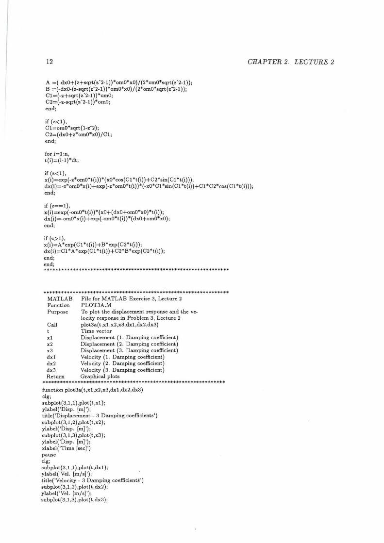
2.1.2 MATLAB Files ****************************************************************


Call b a k m c n dt xO dxO Return X

dx

File for MATLAB Exercise 3, Lecture 2 EXERC3 .M To calculate the displacement and velocity response of the system in the spring point of the system in problem 3, lecture 2. exerc3(b,a,k,m,c,n,dt,xO,dxO) (see fig . Prob. 3) Length of stucture Distance to mass and damping Stifness of linear spring Mass Damping constant Number of points in discrete time Time difference between points Initial displacement Initial velocity/ eigenfrequency (x,dx,t) Displacement response vector Velocity response vector Time vector

**************************************************************** function [x,dx,t]=exerc3(b,a,k,m,c,n,dt,xO,dxO)

omO=(b/a)*sqrt(k/m); z=c/ (2*sqrt(k*m) ); xO=xO*a; dxO=dxO*omO*a;

if (z>l),

11

12

A=( dxO+(z+sqrt(z·2-l)}*omO*x0)/(2*omO*sqrt(z·2-l)); B =( -dx0-(z-sqrt(z·2-1) )*omO*xO) /(2*omO*sqrt(z·2-l) ); Cl=(-z+sqrt( z·2-1) )*omO; C2=( -z-sqrt(z·2-1) )*omO; end;

if (z<l), Cl=omO*sqrt(l-z.2); C2=( dxO+z*omO*xO)/Cl; end;

for i=l:n, t(i)=(i-l)*dt;

if (z<l),

CHAPTER 2. LECTURE 2

x(i)=exp( -z*omO*t(i))*(xO*cos(Cl *t(i) )+C2*sin(Cl *t(i))); dx(i)=-z*omO*x(i)+exp( -z*omO*t(i) )*( -xO*Cl *sin(Cl *t(i))+Cl *C2*cos(C1 *t(i))); end;

if (z==1), x(i)=exp( -omO*t(i) )*(xO+( dxO+omO*xO)*t(i) ); dx(i )=-omO*x (i)+exp(-omO*t(i) )*( dxO+omO*xO); end;

if (z>l), x(i)=A *exp(C1 *t(i))+B*exp(C2*t(i)); dx(i)= Cl *A *exp(Cl *t(i))+C2*B*exp(C2*t(i)); end; end; ****************************************************************


Call

xl x2 x3 dxl dx2 dx3 Return

File for MATLAB Exercise 3, Lecture 2 PLOT3A.M To plot the displacement response and the velocity response in Problem 3, Lecture 2 plot3a(t,x1 ,x2,x3,dx1 ,dx2,dx3) Time vector Displacement (1. Damping coefficient) Displacement (2. Damping coefficient) Displacement (3. Damping coefficient) Velocity (1. Damping coefficient) Velocity (2. Damping coefficient) Velocity (3. Damping coefficient) Graphical plots

*************************************************************** flUlction plot3a( t,x1 ,x2,x3,dx1 ,dx2,dx3) clg; subplot(3,1 ,1) ,plot(t,x1); ylabel( 'Disp. (m]'); title('Displacement - 3 Damping coefficients ') subplot(3, 1 ,2) ,plot(t ,x2); ylabel( 'Disp. [m]'); subplot(3,1 ,3) ,plot(t,x3); ylabel('Disp. [m]') ; xlabel('Time [sec]') pause clg; subplot(3,1 ,1) ,plot(t,dx1 ); ylabel('Vel. [m/s] '); title('Velocity- 3 Damping coefficient~') subplot( 3,1 ,2) ,plot( t ,dx2); ylabel( 'Vel. [m/s] '); subplot(3,1 ,3) ,plot(t ,dx3);


ylabel('Vel. (m/s]'); xlabel('Time (sec]') ****************************************************************


Call

x1 x2 x3 dx1 dx2 dx3 Return

File for MATLAB Excercise 3, Lecture 2 PLOT3B.M To plot the displacement response and the velocity response in Problem 3, Lecture 2 plot3b(t,xl ,x2,x3,dxl ,dx2,dx3) Time vector Displacement (1. Damping coefficient) Displacement (2. Damping coefficient) Displacement (3. Damping coefficient) Velocity (1. Damping coefficient) Velocity (2. Damping coefficient) Velocity (3. Damping coefficient) Graphical plot

**************************************************************** function plot3b(t,xl ,x2,x3,dxl ,dx2,dx3) clg; subplot(3,1 , 1 ),plot(t,xl); ylabel('a) Disp. (m]'); title( 'Displacement - 3 different initial velocity') grid; subplot(3,1 ,2) ,plot(t,x2); ylabel( 'b) Disp. (m]'); grid; subplot(3,1 ,3),plot(t ,x3) ; ylabel( 'c) Disp. (m) '); xlabel('Time (sec]'); grid; pause clg; subplot(3,1 ,1) ,plot(t,dxl ); ylabel( 'a) Vel. (m/s]'); title( 'Velocity - 3 different initial velocity') grid; subplot( 3,1 , 2) ,plot ( t,dx2 ); ylabel('b) Vel. (m/s]'); grid; subplot(3, 1,3) ,plot(t,dx3); ylabel('c) Vel. [m/s)'); xlabel('Time [sec]'); grid; ****************************************************************

13

Chapter 3

Lecture 3

Problem 1,3 and 4 of lecture 3 are solved theoretically. The solutions to these problems can be found in Nielsen [2). The following MATLAB exercise replaces the corresponding problem 2 of lecture 3.


Verify that the equation of motion of a linear viscous single degree-of-freedom system can be written on the following state vector form :

~ [ ~~!~ ] = [ - ~x(t~(~ ~ x(t) ] + [ ~ ] ~ focos(wt ) (3.1)

Where the initial conditions are:

x(O) = xo , x(O) = xo (3.2)

Assume the initial values of the displacement and velocity of problem 1, lecture 3 are: x 0 = x0 = 0.

Verify upon insertion in the equation of motion and the initial conditions that the solution becomes:

x(t) = IX! [cos(wt- w)- e-(wot (cos('ll)cos(wdt) + sin(wdt) ( ~ + ~sin('ll))) l (3 .3) 1- (2 Wd

Where lXI , 'l1 are the amplitude and phase angle of the stationary harmonic motion, w0 , wd are the undamped and damped circular eigenfrequency, ( is the damping ratio determined in problem 1, lecture 3 and w is the frequency of the force. The velocity response is :

x(t) = lXI[ -wsin(wt- w) + (w0e-(wot(cos(\lf)cos(wdt) + sin(wdt)((c~ + ~sin(\lf)))-

v 1-(2 Wd

e-(wot( -wdcos('ll)sin(wdt) + wdcos(wdt)( (c~ + ~sin(\lf))] V 1-(2 Wd

(3.4)

Solve (3.1) numerically using a 4th order Runge-Kutta scheme and compare the solution with the analytical solution (3.3). Use the following data:

2 N kg 0.327r2 N w = wo = 21rHz, k = 01r - , m= lkg, a= 1m, c = 0.047r-, / o = (3.5)

· m s 3 Plot the force versus the displacement and velocity response of the system for different frequencies of the force , w.

14

3.1. MATLAB EXERCISE 4 15


The MAT LAB functions below ( exerc4a.m, plot4a.m) shows how MAT LAB exercise 4, lecture 3 could be solved . If the following three orders are given :

{tl ,x1, dx1 , tt,xt, dxt}= exerc4 a{16*pi' 2, 0. 04 *pi, 1, 0. 32*pi' 2/3, 2*pi,4 0, 0. 25); [t2, x2, dx2, tt, xt, dxt}= exerc4 a( 16*pt 2, 0. 04 *pi, 1, 0. 32*p( 2/3, 2*pi, 100, 0.1 ); [t3,x3, dx3, tt,xt, dxt}= exerc4 a{16*pt 2, 0. 04*pi,1, 0.32*pt 2/3, 2*pi, 200, 0. 05 ); plot4 a{t1, t2, t2,x1,x2,x3, dx1, dx2, dx3, tt, xt, dxt);

Then figure 3.1 and figure 3.2 will appear on the screen. Notice that "RETURN" should be pressed to shift from figure 3.1 to figure 3.2. An explanation of the input numbers can be found in the top of the MATLAB functions (exerc4a.m, plot4a.m). Notice that the numerical approximation converges as the time intervals decreases.

r: -o·5o 1 2 3 4 5 6 7 8 9 .. 10

- '·' E : : : ; : : : : : -- : : : : : : : : : . . . . . . . . .

~'= -o.so 1 2 3 -4 5 6 7 8 9 . 10

- ' ·' e : : : : : : : : : ....... : : : : : : : : : . . ' . . . . . .

~'= -o· 5o 1 2 3 4 5 6 7 8 9 10 Tirne [sec]

Figure 3.1 : Numerical approximation [-} of the displacement with a fourth order Runge-Kutta scheme and theoretical so lution[ .. ]. a) L\t=1f, b) L\t=tg, c) L\t=fg.


Velocity - 3 Different time intervals

r -~~---1L---~2~--~3----~4----~5----~6----,~--~8~--~9----~1o·

~: -~~--~1 --~2~--~3~--~4----~5----~6----~,--~8~--~9~~10

~ -~~---1L---~2~--~3----~4----~5----~6--~7~---8L---~9--~10

Time [sec)

Figure 3.2 : Numerical approximation [-]of the velocity with a fourth order Runge-Kutta scheme and theoretical solution[..]. a) D..t='Jf , b) D...t=~, c) D...t=~.

To plot the force versus the displacement and velocity response with different frequencies of t he force, perform the following 2 examples.

Example 1: w = 2.05w0 . If the MATLAB files exerc4b.m and plot4b.m where implemented, the following two orders should be given:

[t,xt, dxt, Ft]=exerc4b{16*pt 2, 0. 04 *pi, 1, 0.32*pi' 2/3,2. 05*pi,400, 0. 05 }; plot4 b(t, xt, dxt, Ft};

Then the following graph will appear on the screen:


Comparison: force-Response I

~M ...... .:. . . .. . : ..... ...... .. ..... ' ........ L ....... [ ...... ;.. ........ :. ...... . L ...... . V ; ; , . ; : ; t~JJIMIMM/lMIM

0 2 4 6 8 I 0 12 1-4 16 I 8 20

0, : : . . : : : : .

~ . . . . . . . . . e : : : : : : : : :

~'~ -o· 5o 2 4 6 8 10 12 1-4 16 18 20

: : : : : : : : : E' 2 ........... : ............ , ........... : ......... : ....... : ........ ; ....... : . ....... : ........ : ..... · ...... ; : : : : : : . . . . . . . . . . . . . . . .

~-- 4o 2 4 6 8 10 12 14 16 18 20

Time [sec)

Figure 3.3: Response of system subjected to a harmonic force where wo < w. a) Harmonic excitation process, b) displacement response c) velocity response.

Example 2: w = 2.0571'. If the MATLAB files exerc4c.m and p lot4b.m where implemented, the following two orders should be given:

{t,xt, dxt ,Ft}=exerc4c{16*pi' 2, 0. 04*pi,J, 0.32*pi' 2/3, 1. 95*pi,400, 0. 05 }; plot4 b(t, xt, dxt, Ft};

Then the following graph will appear on the screen:

I Comparison: Force-Response

~o.5 ....... . : . .. . . ...................... ' ... ...... . : ........ L .... .i . ...... L .... .. L . .. . ..

~~-MAl-. . . . . .

(.1 : : • . : : ;

o 2 4 6 8 10 12 14 16 18 20

,., . . . . . . . . .

~ . . . . . . . . . E : : : : : : : : : _, : : : : : ; ; : : . : : : : : : : : :

~'= -o. 5o 2 4 6 8 I 0 12 14 16 I 8 20

l::~:: h: ·Aj i~~ -~~--~2----~4----~6----~8----I~0----1~2----~14----~1 6----~1 8~~20

Time [sec]

Figure 3.4: Response of system subjected to a harmonic force where wo > w. a) Harmonic excitation process, b) displacement response c) velocity response.

18

3.1.2 MATLAB Files

•••••••••••••••••••••••••••••••••••••••••••••••••••••••••••••••• MATLAB Function Purpose

Call k c m fO omf n dt Return xl x2 xt t

File for MATLAB Exercise 4, Lecture 3 EXERC4A.M To calculate the response of the system described in problem 1, lecture 3. A Runge-Kutta fourth order method is used. exerc4a(k,c,m ,fO,ornf,n ,dt) (fig.Prob. 1) Stifness of linear spring Damping constant Mass Amplitude of force Eigenfrequency of harmonic force Number of points in approximtation Time distance between points (x,dx,t) Displacement response vector Velocity response vector Theoretical solution Corresponding time vector

•••••••••••••••••••••••••••••••••••••••••••••••••••••••••••••••• function (t,x1 ,x2,tt ,xt,dxt]=exerc4a(k,c,m,fO,ornf,n,dt)

omO=O.S*sqrt(k/m); z=c/sqrt(m*k);

constants used in differential equation Cl=om0-2; C2= 2*z*om0; C3= (0. 75*f0) /m; for l=1:n+l , xl(l)=O; x2(l)= O; t(l)=O; end;

xl(l)= O; Initial conditions- zero displacement x2(1 )=0; Initial conditions- zero velocity t(l )=0;

for l=l :n, kl=O.S*dt*(-Cl *x1 (l)-C2*x2(l)+C3*cos( ornf*t(l)) ); K=O.S *dt* (x2(l)+0.5*kl) ; k2= 0.5*dt*(-Cl *(x1 (l)+K)-C2*(x2(l)+kl )+C3*cos( ornf*( t(l)+0.5*dt))); k3= 0.5 *dt *(-Cl* (xl (1 )+ K)-C2*( x2 (I)+ k2 )+C3*cos( ornf*( t(l)+O.S*dt))); LL=dt*(x2(l)+k3); k4= 0.5*dt*(-Cl *(x1 (l)+LL)-C2*(x2(1)+2*k3)+C3*cos( ornf*( t(l)+dt))); xl (1+ 1 )=xl(l)+dt*(x2(1)+(1/3)*(kl +k2+k3) ); x2(l+ 1 )=x2(l) +(1 /3 )* (k1 + 2*k2+ 2*k3+k4); t(l+l)=t(l)+dt; end; theoretical solution if ( omO==ornf) psi=pi/2; else psi=atan( (2*z *omO*ornf) / ( om0-2-ornf'2)); end; X=(O. 75*fO)/ (m*sqrt( ( om0"2-ornf'2P+4*(z"2)*( om0"2)*( ornf'2))); omd= omO*sqrt (1-z "2);

laengde=n *dt; dt=laengde/2000; n=2000;

for l= l:n+1, tt(l)= (l-1) *dt; Displacement response xhl =cos( ornf*tt(l)-psi); xh2=cos(psi)*cos( omd*tt(l)); xh3=sin( omd*tt(l))*( (z*cos(psi) )/ (sqrt(l-z"2) )+ ( omf/ omd)*sin(psi));



xt(l) =X* ( xh1-exp( -z*omO*tt(l)) *( xh2+xh3)); Velocity response dxh 1 =-ornf*sin( omf*tt(l)-psi); dxh2=xh2; dxh3=xh3; dxh4=-omd*cos(psi) *sin( omd*tt(l)); dxhS=omd*cos( omd*tt(l) )* ( ( z*cos(psi)) / (sqrt(1-z·2)) + ( omi/ omd)*sin(psi)); dxt (l)=X* ( dxh1 +z*omO*exp( -z*omO*tt(l) )*( dxh2+dxh3)-exp( -z*omO*tt(l) )* ( dxh4+dxh5) ); end; ****************************************************************

**************************************************************** MATLAB FUnction Purpose

Call tl t2 t3 x1 x2 x3 dxl dx2 dx3 tt xt dxt Retum

File for MATLAB Exercise 4, Lecture 3 PLOT4A.M To plot the displacement response and the velocity response in Problem 1, Lecture 4 plot4a( t 1 ,t2 ,t3 ,xl ,x 2,x3,dx1 ,dx2 ,dx3,tt,xt,dxt) Time vector Time vector Time vector Displacement (1. Damping coefficient) Displacement ( 2. Damping coefficient) Displacement (3. Damping coefficient) Velocity {1. Damping coefficient) Velocity (2. Damping coefficient) Velocity (3. Damping coefficient) Time vector Theoretical Displacement Theoretical Velocity Graphical plot

**************************************************************** function plot4a( tl,t2 ,t3,x1 ,x2,x3,dx1 ,dx2,dx3,tt,xt,dxt) clg; subplot(3,1, 1) ,plot(t1 ,x1 ,tt ,xt, ':'); ylabel('a) Dbp. (m]'); title('Displacement- 3 Different time intervals') grid; axis((O 10 -0.5 0.5]); subplot(3, 1 ,2) ,plot( t 2,x2 ,tt ,xt,': '); ylabel('b) Disp. (m]') ; grid; axis((O 10 -0.5 0.5]); subplot(3,1,3) ,plot(t3,x3, tt,xt,' :' ); ylabel('c) Disp. (m]'); grid; axis((O 10 -0.5 0.5]) ; pause clg; subplot(3,1,1) ,plot(tl,dxl,tt ,dxt, ': '); ylabel('a) Vel. [m/s]'); title('Velocity- 3 Different time intervals') grid ; axis((O 10 -5 5]); subplot(3,1,2) ,plot(t2 ,dx2,tt,dxt,': '); ylabel( 'b) Vel. (m/s]'); grid; a.xis((O 10 -5 5]); subplot(3,1,3) ,plot(t3,dx3,tt,dxt, ': '); ylabel('c) Vel. (m/s]'); grid ; axis((O 10 -5 5]);

****************************************************************

19

20

****************************************************************


Call k c m fO omf n dt Return tt xt dxt Ft

File for MATLAB Exercise 4, Lecture 3 EXERC4B.M To calculate the response of the system described in problem 1, lecture 3. A Runge-Kutta fourth order method is used. exerc4b(k,c,m,fO,omf,n,dt) (fig.Prob. 1) Stifness of linear spring Damping constant Mass Amplitude of force Eigenfrequency of harmonic force Number of points in approximtation Time distance between points (tt,xt,dxt,Ft) Time vector Displacement response vector Velocity response vector Force vector

**************************************************************** function (t t ,xt ,dxt,Ft J =exerc4b(k,c,m,fO,omf,n,dt)

om0=0.5*sqrt (k/ m); z= c/sqrt(m*k);

if ( omO==omf) psi= pi/2; else psi=atan( (2*z*omO*omf) I ( omo·2-omi2)); end; X=(O. 75*f0)/ (m*sqrt(( om0·2-omi2P+4 *(z.2)*( om0.2)*( omi2))); omd=omO*sqrt(1-z·2);

laengde=n*dt; dt=laengde/4000; n=4000;

for 1= 1:n+l , tt(l)=(l-1)*dt; Displacement response xh1 =cos( omf*tt(l)-psi); xh2=cos(psi)*cos( omd*tt(l)); xh3=sin( omd*tt(l) )*( (z*cos(psi) )I (sqrt(1-z.2) )+( omfl omd)*sin(psi) }; xt (I) =X* ( xh1-exp( -z *omO*tt (1)) * ( xh2+xh3)); Velocity response dxhl=-omf*sin( omf*tt(l )-psi); dxh2=xh2; dxh3= xh3; dxh4=-omd*cos(psi)*sin( omd*tt(l)); dxh5=omd*cos( omd *tt (l)) * ( ( z*cos(psi)) I (sqrt(l -z·2)) +( omf/ omd) *sin(psi));


dxt(l)=X*( dxh1 +z*omO*exp( -z*omO*tt(l) )*( dxh2+dxh3)-exp(-z*omO*tt(l) )*( dxh4+dxh5)); Ft(l)=cos( omf*tt(l) ); end; ****************************************************************


****************************************************************


Call

xt dxt Ft Return

File for MATLAB Exercise 4, Lecture 3 PLOT4b.M To plot the displacement response and the velocity response versus the force on the system in Problem 1, Lecture 4 plot4b{t,xt,dxt,Ft) Time vector Displacement Velocity Force applied to the system Graphical plot

****************************************************************

function plot4b{ t,xt,dxt,Ft) clg; subplot(3,1 ,l),plot(t,Ft ); ylabel('a) Force (N]'); title('Comparison: Force-Response'); grid; subplot(3,1 ,2) ,plot(t ,xt); ylabel('b) Disp. (m] '); grid; subplot{3,1 ,3) ,plot(t,dxt ); ylabel('c) Vel. (m]'); xlabel('Time (sec]') grid; ****************************************************************

****************************************************************


Call k c m fO omf n dt Return tt xt dxt Ft

File for MATLAB Exercise 4, Lecture 3 EXERC4C.M To calculate the response of the system described in problem 1, lecture 3. A Runge-Kutta fourth order method is used. exerc4c{k,c,m,fO,omf,n,dt) {fig.Prob. 1) Stifness of linear spring Damping constant Mass Amplitude of force Eigenfrequency of harmonic force Number of points in approximtation Time distance between points (tt ,xt,dxt,Ft) T ime vector Displacement response vector Velocity response vector Force vector

**************************************************************** function ( tt ,xt ,dxt,Ft ]=exerc4c{k,c,m ,fO,omf,n,dt) om0=0.5*sqrt{k/m); z=c/sqrt{m*k); if (omO==omf) psi=pi/2; else psi=atan( {2*z*omO*omf) I ( omo·2-omi2)); end; X= (O. 75*f0)/ (m*sqrt( ( om0·2-omi2)"2+4*( z-2 )*( om0-2)*( omi2))); omd=omO*sqrt(I-z'2); laengde= n*dt; dt= laengde/4000; n= 4000; for l= l :n + I , tt(l)= (l-l)*dt ;

21

22

xhl=cos( omf*tt(I)-psi); xh2=cos(psi )*cos( ornd *tt (I)) ; xh3=sin(omd*tt(I))*( (z*cos(psi) )/ (sqrt(l-z-2))+( omf/ omd)*sin(psi)) ; xt (I) =X* ( xhl-exp( -z *ornO* tt (I))* ( xh2+xh3)) ; dxhl=-omf*sin{ omf*tt(l)-psi); dxh2=xh2; dxh3=xh3; dxh4=-omd*cos(psi)*sin( omd*tt(l) ); dxhS=omd*cos{ omd *tt(I)) *( ( z*cos(psi)) / ( sqrt (l-z·2) )+( omf/ omd) *sin(psi)) ;


dxt(I )=X*( dxhl +z *ornO*exp{ -z*omO*tt(l) )*( dxh2+dxh3)-exp( -z*omO*tt(I) )*{ dxh4+ dxh5) ); Ft(l)=cos( omf*tt(I) ); end;

Chapter 4

Lecture 4

Problem 1 and 3 of lecture 4 are solved theoretically. The solutions to these problems can be found in Nielsen [2] . The following MATLAB exercises replaces problem 2 of lecture 4.


Determine the eigenvalues >. and eigenvectors 'ili for the following linear eigenvalue problem:

(B - >.A) = 0 ( 4.1)

Where A and B are real and symmetric matrices.

Example 1 (Example 3.5 in Nielsen [1])

B = [ 2 -1 ] -1 2

(4.2)

Compare results with (3.43) , (3.61), and (3.62) in Nielsen [1]. Notice that both A and B are symmetric and positive definite matrices in this case.

Example 2 (Example 3.10 in [1])

[

0.3 -0.2 1 0 ] A _ -0.2 0.5 0 2

- 1 0 0 0 0 2 0 0

0 0

B - -100 200

[

200 -100

- 0 0 -1 0 0 0

(4.3)

Compare the results with (3.197) , (3 .102), (3 .230), (3.239), (3.240) and (3.241) in Nielsen [1].


The MATLAB function below (exerc5a.m) shows how MATLAB exercise 5, lecture 4 could be solved. If the following orders are given:

A(1,1:2)={1 0}; A(2,1:2) ={0 2}; B(1,1:2)={2 -1}; B(2,1:2)={-1 2};

23


[V, D J=exerc5a( A, B };

Then the eigenvalues and corresponding eigenvectors of example 1 will appear on the screen . Notice that the eigenvectors only can be calculated except for an arbitrary constant.

Eigenvalues:

[ 0.60340 0 ]

2.3660

Eigenvectors:

To solve example 2 give the following orders:

A(1,1:4)={0.3 -0.2 1 0}; A(2,1:4)=[-0.2 0.5 0 2}; A{3,1:4)=[1 0 0 0}; A(4,1:4)=[0 2 0 0}; B(1,1:4)={200 -100 0 0}; B(2,1:4)={-100 200 0 0}; B{3,1:4)={0 0 -1 0}; B(4,1:4)={0 0 0 -2}; [V,D}=exerc5b( A,B );

( 4.4)

(4.5)

Notice again that the eigenvectors only can be calculated except an arbitrary constant.

Eigenvalues:

Eigenvectors:

[

o.7321 + o.oo5o;

-0.0933 + 5.8283i - 0.0725 + 7.9620i

0 -0.0725- 7.9620i

0 0

0.7321- 0.0050i 1

-0.0933- 5.8283i -0.0725- 7.9620i

0 0

-0.2025 + 15.3804i 0

-2.7313 + 0.0364i 1

-0.0066- 42.0159i -0.2025 + 15.3804i

0 l 0 0 ( 4.6)

- 0.2025- 15.3804i

-2.7313- 0.0364i l -0.0066 + 42.0159~ ( 4·7) -0.2025- 15.3804i

The eigenvectors are the two first rows in each column. What are the relation between the two last rows in each column and the eigenvalues? (The answer is given in Nielsen [1] p. 77, (3-209)).


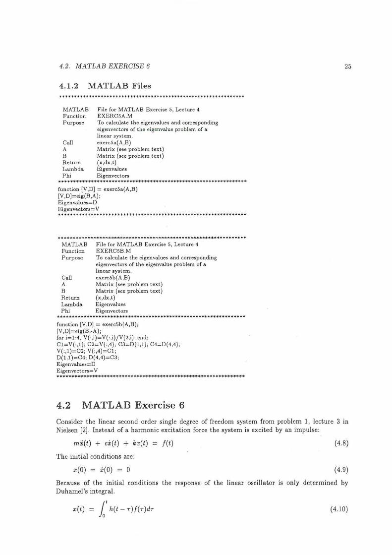
4.1.2 MATLAB Files ***************************************************************

MATLAB File for MATLAB Exercise 5, Lecture 4 Function EXERCSA.M Purpose To calculate the eigenvalues and corresponding

eigenvectors of the eigenvalue problem of a linear system.

Call exerc5a (A,B) A Matrix (see problem text) B Matrix (see problem text) Return (x,dx,t) Lambda Eigenvalues Phi Eigenvectors

**************************************************************** function [V ,D] = exerc5a(A,B) [V,DJ=eig(B,A); Eigenvalues=D Eigenvectors= V ****************************************************************


File for MATLAB Exercise 5, Lecture 4 EXERCSB.M To calculate the eigenvalues and corresponding eigenvectors of the eigenvalue problem of a linear system.

Call exercSb(A,B) A Matrix (see problem text) B Matrix (see problem text) Return (x,dx,t) Lambda Eigenvalues Phi Eigenvectors

**************************************************************** function [V,D) = exerc5b(A,B); [V,D)=eig(B ,-A) ; for i=l:4, V(:,i)= V(:,i)/V(2,i); end ; Cl=V(:,l) ; C2=V(:,4) ; C3=D(l,l); C4=D(4,4); V(:, l )=C2; V(:,4)=Cl; D(l,l)=C4; D(4,4)= C3; Eigenvalues=D Eigenvectors=V ****************************************************************


25

Consider the linear second order single degree of freedom system from problem 1, lecture 3 m Nielsen [2). Instead of a harmonic excitation force the system is excited by an impulse:

mi(t) + cx(t) + kx(t) = f(t) (4.8)

The initial conditions are:

x(O) = x(O) = 0 (4.9)

Because of the initial conditions the response of the linear oscillator 1s only determined by Duhamel's integral.

x(t) = it h(t - r)f(r)dr (4.10)


The impulse excitation is shown in figure 7 .2.

f(T)

a

l>t

Figure 4.1: Impulse excitation of a linear single degree of freedom system.

The analytical solution to the vibration problem can be found in Appendix A. Verify upon insertion in the equation of motion ( 4.8) that the solutions for t ::; !:it becomes:

(4.11)

Solve ( 4.8) numerically using a 4th order Runge-Kutta scheme and compare the solutions with the analytical solution (4.11). Use the following data:

2N k = 1671" - , m= 1kg ,

m

kg c = 0.0471"-)

s a= 1N, !:it = 0.5s (4.12)

Plot the displacement and the velocity response of the system for different approximations.

Solve (4.10) using Simpson integration. Compare the solution with the analytical solution (4.11). Use the data from ( 4.12). Plot the displacement of the system for different approximations. It is important to notice that the vibration problem can be solved using two different approaches: A numerical approximation of the differential equations or a numerical integration of the Duhamel integral.


The MATLAB functions below (exerc6a.m, plot6a.m) shows how the numerical approximation of the differential equation in MATLAB exercise 5, lecture 4 could be performed. If the following four orders are given:

{tl,x1, dx1, tt,xt, dxt}=exerc6a{16*pt 2, 0. 04 *pi, 1,1, 0.5, 25, 0.2}; {t2,x2, dx2, tt,xt, dxt]=exerc6a{16*pi" 2, 0. 04*pi, 1,1, 0.5, 50, 0.1}; [t3,x3, dx3, tt,xt, dxt]=exerc6a{16*pi" 2, 0. 04 *pi, 1, 1, 0.5, 1000,0. 005); plot6a{t1, t2, t3,x1 ,x2,x3, dx1, dx2, dx3, tt,xt, dxt);

Then figure 4.2 and figure 4.3 will appear on the screen. Notice that " RETURN" should be pressed to shift from figure 4.2 to figure 4.3. An explanation of the input numbers can be found in the head of the MATLAB functions (exerc6a.m, plot6a.m). Notice how the numerical approximation converges to the theoretical solution as the time intervals decreases .


t Displacement - 3 different approxi mations

-o · 04o~-~o.L.:. 5,---..L1--1:-~.-=-5--.,2~-~2.1.:. 5,---~3--3::-1.'=5--4L---:_..L, 5=---~5

~ 0.04 . : : ; : : ; : :

~ 0 . 02 .. . , ... .. : ··· · ···<··········· :····· ...... ; .......... >· ··· ····'··········> ·······;···· ·· ... ·: .. .... . . : : : : : : : : : ! 0 ••••• • ••f••••• •• •·•t• ·•••oo '' 't" ''"'' •••~••••••• · •• •~••••• •• ''''t''""' • ••~ •• •••••• ' "~'''"'' ' •••~•••••• •• •

;-0.02

- o · 04o~-~o.L.:. 5,-----..1.1 __ ,.-~1 .-=-5--.,2~-~2.1.:. 5,----~3--3::-1.'=5--.. ~--:4~. 5=----~5 Time [sec]

27

Figure 4.2: Numerical approximation of the displacement with a fouth order Runge-Kutta scheme compared with theoretical solution. a) At = :?f~ b) At = tfr~ c) A t= fat.

'·'

~~:~ -o.~ 0.5 1 1 .5 2 2.5 3 3 . 5 4 4 . 5 5

'·' i o. 1 .. . ...... : .......... , .. .. .... ...... . .. : .. ..... . ; ..... ....... [ ..... · .. . :.. ......... .. . .... : ·· .... .

...; 0 .......... ~ .......... ~ .......... , .......... :. .... ..~. . ........ ; .......... , ...... ..... ; ..... .... : ....... ..

;-0 . 1

-o .~ 0 .5 . 1 1.5 2 2 .5 3 3.5 4 4. 5 5

"' i o.1 ...... . .. ' ............ : ......... , ............ L ................... + ... ...... = ........... : .. .. . ... .. · ........ ..

~-0.~ -o.~ 0 . 5 1 1.5 2 2 .5 3 3 . 5 4 4 .5 5

Time [sec]

Figure 4.3: Numerical approximation of the velocity with a fo uth order Runge-Kutta scheme compared with theoretical solution. a) At = :?f 1 b} A t = fg 1 c) A t = fat .

The MATLAB functions below (exerc6b.m, plot6b.m) shows how the numerical integration of the Duh amel integral in MATLAB exercise 5, lecture 4 could be performed using Simpson integration . If the following four orders are given:


[t1,x1, tt,xt}=exerc6b{16*pi' 2, 0. 04*pi, 1, 1, 0.5, 25, 0.2);

{t2,x2, tt, xt}=exerc6b{16*pt2, 0.04*pi, 1, 1, 0.5,50, 0.1);

{t3,x3, tt,xt)=exerc6b{16*pt 2, 0. 04*pi, 1, 1, 0. 5,1 00, 0. 05);

plot6b{t1, t2, t3,x1, x2,x3, tt, xt};

Then figure 4.4 will appear on the screen. An explanation of the input numbers can be found in the head of the MATLAB functions (exerc6b.m, plot6b.m). Notice how the numerical approximation converges to the theoretical solution as the time intervals decreases.

O. M

;_:::~ -o . o~o 0.5 1 1.5 2 2 .5 3 3 .5 4 4. 5 5

i-: -o. 0~o=---=-o"=.5---:1~-:-'1 .-=-:; ---=2-----::2~. 5::----:!:-3-~3"-:. 5;---4~--:-'4 .'=5-~5

!: -o · 0~o=---=-'o .Lo-5----:1'----1,.....-=-5 ---=2----=2'"'"'. 5:----:!:-3 -----=-3-'--=. 5,----4~-.,-14 .-=5---:'5

Time [sec]

Figure 4.4: Numerical approximation of the displacement calculated using Simpson integration compared with theoretical solution. a) !lt = :If' b) !lt = n' c) !lt = frfo.


4.2.2 MATLAB Files

****************************************************************


Call k c m a dta n

dt Return t xl x2 tt xt dxt

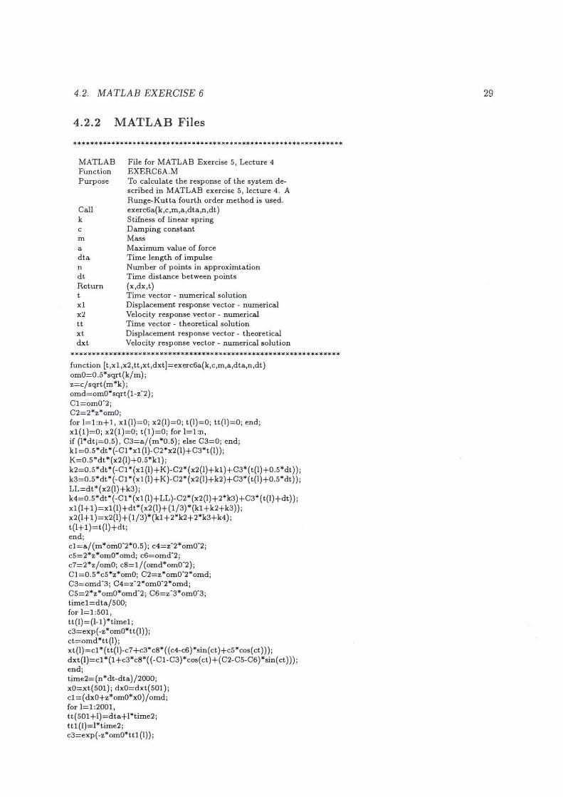
File for MATLAB Exercise 5, Lecture 4 EXERC6A.M To calculate the response of the system described in MATLAB exercise 5, lecture 4. A Runge-Kutta fourth order method is u sed. exerc6a(k,c,m,a,dta,n,dt) Stifness of linear spring Damping constant Mass Maximum value of force Time length of impulse Number of points in approximtation Time distance between points (x,dx,t) Time vector - numerical solution Displacement response vector - numerical Velocity response vector- numerical Time vector - theoretical solution Displacement response vector - theoretical Velocity response vector- numerical solution

•••••••••••••••••••••••••••••••••••••••••••••••••••••••••••••••• function [t ,xl ,x2, tt,xt,dxt )=exerc6a(k,c ,m,a,dta,n,dt) om0=0.5*sqrt(k/ m) ; z=c/sqrt(m*k); omd=omO*sqrt (1-z"2); Cl = om0"2; C2=2*z*om0; for l=l:n+l, xl(l)=O; x2(l)=O; t(l)=O; tt(l)=O; end; xl(l)=O; x2(1)=0; t(1)=0; for 1=1:n, if (l*dtj=0.5), C3=a/(m*0.5); else C3=0; end; k1 =0.5*dt*(-C1 *x1 (l)-C2*x2(l)+C3*t(l) ); K=0.5*dt *(x2(1)+0.5*kl); k2=0.5*dt*(-C1 *(xl(l)+K)-C2*(x2(l)+kl)+C3*(t(l)+0.5*dt)) ; k3=0.5*dt *(-Cl *(xl (l)+K)-C2*(x2(l)+k2)+C3*(t(l)+O.S*dt)); LL=dt*(x2(l)+k3); k4=0.5*dt*( -Cl *(xl (l)+LL )-C2*(x2(1)+2*k3)+C3*( t(l)+dt)); x1 (l+ 1 )=x1 (l)+dt*( x2(l)+ (1 /3)*(kl + k2+k3)) ; x2 (1 + 1 )=x2 (1) + (1 /3)* (k1 + 2*k2+ 2*k3+k4); t(l+ 1 )=t(l)+dt; end; c1=a/(m*om0"2*0.5); c4=z"2*om0"2; c5=2*z*omO*omd; c6=omd"2; c7= 2*z/om0; c8=1/(omd*om0"2); C1=0.5*c5*z*om0; C2=z*om0"2*omd; C3=omd"3; C4=z"2*om0"2*omd; C5=2*z*omO*omd"2; C6=z"3*om0"3; timel=dta/500; for 1=1:501, tt(l)=(l-1 )*time1; c3=exp( -z*omO*tt(l) ); ct=omd *t t (1); xt(l)=c1 *(tt(l)-c7 +c3*c8* ( ( c4-c6)*sin ( et )+cS*cos( et))); dxt(l)= cl *(1 +c3*c8*( ( -C1-C3)*cos( et) +(C2-C5-C6)*sin( et))); end; time2= (n *dt-dta) /2000; xO=xt(501); dx0=dxt(501); c1= (dxO+ z*omO*xO)/omd; for 1= 1 :2001, tt(501+l)= dta+l*time2 ; ttl(l)= l*time2; c3= exp( -z*omO*ttl (1)) ;

29

30

ct=omd*ttl(l); xt(SOl +l) =c3*(xO*cos( ct)+cl *sin(ct)); dxt( SOl +1)=-z*omO*xt( 501 +l)+c3*omd*(-xO*sin( et )+cl *cos( et)) ; end; ****************************************************************


Call t1 t2 t3 xl x2 x3 dxl dx2 dx3 tt xt dxt Return

File for MATLAB Exercise 5, Lecture 4 PLOT6a.M To plot the displacement response and the velocity response in MATLAB Exercise 5, lecture 4 plot6a(t1 ,t2 ,t3,xl ,x2,x3,dxl ,dx2,dx3,tt,xt,dxt) Time vector (1. Aproximation) Time vector (2. Aproximation) Time vector (3. Aproximation) Displacement (1. Aproximation) Displacement (2. Aproximation) Displacement (3. Aproximation) Velocity (1. Aproximation) Velocity (2. Aproximation) Velocity (3. Aproximation) Time vector Theoretical Displacement Theoretical Velocity Graphical plot

**************************************************************** function plot6a( t1 ,t2,t3,xl ,x2 ,x3,dx1 ,dx2,dx3,tt,xt,dxt) clg; subplot(3,1, 1) ,plot(tl ,xl ,tt ,xt, ':'); ylabel('a) Disp. [m] '); axis([O 5 -0.04 0.04]); title( 'Displacement - 3 different approximations') grid; subplot(3,1 ,2) ,plot(t2 ,x2,tt,xt, ':'); ylabel( 'b) Disp. [m]'); axis([O 5 -0.04 O.D4]); grid; subplot(3,1 ,3) ,plot(t3 ,x3,tt,xt, ': ') ; ylabel( 'c) Disp. [m]'); xlabel( 'Time [sec]'); axis([O 5 -0.04 0.04]); grid; pause clg; subplot(3,1 ,1) ,plot(tl ,dx1 ,tt ,dxt, ':'); ylabel( 'a) VeL [m / s]'); title( 'Velocity- 3 Different approximations') axis([O 5 -0.2 0 .2]) ; grid; subplot(3,1 ,2) ,plot(t2 ,dx2,tt,dxt, ': '); ylabel('b) VeL [m/s]'); axis([O 5 -0.2 0.2]); grid; subplot(3, 1 ,3) ,plot(t3,dx3,tt ,dxt, ' : '); ylabel('c) VeL [m/s]'); xlabel('Time [sec]'); axis([O 5 -0.2 0 .2]); grid; ****************************************************************



**************************************************************** MATLAB FUnction P=pose

Call k c m a dta n dt RetW'n t x1 tt xt

file for MATLAB Exercise 5, LectW'e 4 EXERC6B.M To calculate the response of the system described in MATLAB exercise 5, lectW'e 4. Simpsons integration method is used for Duhamels integral exerc6b(k,c,m,a,dta,n,dt) Stifness of linear spring Damping constant Mass Maximum value of force Time length of impulse Number of points in approximation Time distance between points (t,x1,tt,xt) Time vector - numerical solution Displacement response vector - numerical Time vector - theoretical solution Displacement response vector - theoretical

**************************************************************** function [t,x1,tt,xt)=exerc6b(k,c,m,a,dta,n,dt)

om0= 0.5*sqrt(k/m); z=c/sqrt(m*k) ; omd=omO*sqrt(1-z·2);

C1=1/(m*omd) ; for i= l:n+1, x1(i)=O; t(i)=O; end; for i=1:n , ta=i*dt ; for j=l:i, if (j*dtt.dta) , a1= 0; else a1 =a; end; tl=(j-1)*dt ; t2= tl+0.5*dt; t 3=tl+dt ; g1=C1 *exp(-z*omO*(ta-tl ))*sin(omd*(ta-tl))*a1 *tl/dta; g2= Cl *exp(-z*omO*(ta-t2))*sin( omd*(ta-t2))*al *t2/dta; g3=C1 *exp(-z*omO*(ta-t3) )*sin( omd*( ta-t3) )* a1 *t3/ dta; simpsum=(g1+4*g2+ g3) ; xl(i+l)=xl(i+l)+simpsum; end; x1 (i+ 1 )=ta*x1(i+ 1) /(3*(2*i-1 )) ; t(i+1)=i*dt; end;

c1=a/(m*om0.2*0.5); c4=z·2*om0"2 ; c5=2*z*omO*omd; c6=omd.2; c7= 2*z/om0; c8=1/(omd*om0.2); C1=0 .5*c5*z*om0; C2=z*om0.2*omd; C3=omd .3; C4= z·2*om0.2*omd; C5=2*z*omO*omd.2; C6=z-3*om0.3;

time1::dta/500;

for 1= 1:501, tt(l)=(l-1 )*time1; c3=exp(-z*omO*tt(l) ); ct=omd *tt(l) ; xt(l)=c1 *( tt(l)-c7 +c3*c8*( ( c4-c6)*sin( et )+c5*cos( et))); end; dxO=c1 *(1 +c3*c8*( ( -C1-C3) *cos( et)+( C2-C5-C6)*sin( et))); time2= ( n *dt-dta) /2000;

xO= xt(501) ; cl=(dxO+z*omO*xO)/omd;

31

32

for 1=1:2001, tt( 501 +l)=dta+l*time2; ttl(l)=l*time2; c3=exp( -z*omO*tt1 (1)); ct=omd*tt1(1); xt( 501+l)=c3*(xO*cos( ct)+cl *sin( et)); end; ****************************************************************


Call t1 t2 t3 xl x2 x3 tt xt dxt Return

file for MATLAB Exercise 5, Lecture 4 PLOT6B.M To plot the displacement response MATLAB Exercise 5, lecture 4 plot6b(tl,t2,t3,x1,x2,x3,tt,xt,dxt) Time vector (1. Aproximation) Time vector (2. Aproximation) Time vector (3. Aproximation) Displacement (1. Aproximation) Displacement (2. Aproximation) Displacement (3. Aproximation) Time vector

· Theoretical Displacement Theoretical Velocity Graphical plot

**************************************************************** function plot6b{tl,t2,t3,xl,x2,x3,tt,xt) clg; subplot(3,1,1) ,plot(tl,xl,tt,xt,':'); ylabel('a) Disp. (m]'); axis([O 5 -0.04 0.04)); title('Displacernent- 3 different approximations') grid; subplot(3,1,2) ,plot(t2,x2,tt,xt,':'); ylabel('b) Disp. (m]'); axis((O 5 -0.04 0.04)); grid; subplot(3,1 ,3) ,plot(t3,x3,tt ,xt, ' : '); ylabel('c) Disp. [m]'); xlabel('Time (sec]'); axis((O 5 -0.04 0.04)); grid; ****************************************************************


Chapter 5

Lecture 5

Problem 2 of lecture 5 is solved theoretically. The solutions to these problems can be found in Nielsen (2]. The following MAT LAB exercise replaces problem 1 of lecture 5.


The system of problem 2, lecture 5 is considered . The equation of motion and the initial conditions are :

MX: + Kx = o , t > o (5.1)

x o = [ i ] , xo = [ ~ ] (5.2)

Verify that (5.1) can be written in the following state vector form :

z = Az , z(O) zo (5.3)

[ x(t) ]

z(t) = x(t) ' (5.4)

Solve (5 .4) numerically using a 4th order Runge-Kutta scheme and compare the solution with the analytical solution (see Nielsen [2], p . 36, (12)). Use the following data:

m1 = 1kg, m2 = 2kg (5 .5)

The eigenfrequencies can be found in Nielsen [2], p. 35 (3).


The MATLAB functions below (exerc7.m, plot7.m) shows how MATLAB exercise 7, lecture 5 could be solved. If the following three orders are given:

{x1,xt,t1,tt]= exerc7(8*pt2,16*pt2,1,2,{11/3}, {0 0},25,0.2); [x2,xt, t2,tt}=exerc7(8*pt2,16*pt2,1,2,{11/3}, {0 0},50,0.1); plot 7(t1, t2, tt, xJ, x2,xt); Then figure 5.1 will appear on the screen. An explanation of the input numbers can be found in the head of the MATLAB functions (exerc7.m, plot7.m)

33


Displacement - 2 different approximations

i~_j~ 0 0.5 I 1. 5 2 2.5 3 3 . 5 4 4.5 5

~'~ ~ 0.5 . .. ..... .. . : ............ : ... ........ . : ............ : .... ... . .. . . : .. .......... : ........... ; .. .......... : ... ...... . .. : .. ..... .. ..

~ 0 ::::.··· · - ~ ······<: .. :f ... ·.·:.--~ .. - -~· - · ··.·<·.·.· .. !--... -.. : ····-~- - - -,- ·<:: .. 1.- -:> .... . j ... .......... - .- : .~ .. :::. ·· · -~ -- --.- :· · : :: :

~-0~~ 0 0.5 I 1 .5 2 2 .5 3 3.5 4 4 .5 5

~'~ ~ 0.5 .... .. .... , .... .... ... ; ... .... . ; ....... . . : .. . .... .... : .. .. .... ... : ..... .. ... : ... ...... : .. ........ . : ........ .. . . . . . . ' . . .

fit 0 .... .. .... ~ .. .. . . ..... ~ .. ... ·· · · · · ·~-- .. -· .. ... ~ - -- · · · · · · ·- ~· - · · · · · ··· - ~· •»• • ···· ··! .. ···· · · · ·- ~ · -··· .... .. ~·-· · ·· ... .

~-0~~ 0 0.5 I 1.5 2 2 5 3 3.5 4 4.5 5

_,~

i~J~ 0 0 . 5 I I .5 2 2 .5 3 3.5 4 4 .5 5

Time

Figure 5.1: Numerical approximation{-} with a fourth order Runge-Kutta scheme compared with the theoretically solution r . I a) Llt = Jt 2. storey b) Llt = 'If 1. storey c) Llt = fg 2. storey

T . d) tlt = fg !.storey.

5.1.2 MATLAB Files ****************************************************************


Call k1 k2 m1 m2 xO dxO n dt Return xn xt tn tt

File for MATLAB Exercise 7, Lecture 5 EXERC7.M To calculate the response of the 2DOF system described in problem 2, lecture 5. A RungeKutta fourth order method is used. exerc7(k1 ,k2,ml ,m2,xO,dxO,n,dt) (fig.prob. 2) Stifness of upper storey Stifness of lower storey Mass of upper storey Mass of lower storey Initial conditions vector, displacement Initial conditions vector, velocity Number of points in approximtation Time distance between points (xn,xt,tn,tt) Displacement response matrix (approximation) Displacement response matrix (Theoretically) Time vector corresponding to xn Time vector corresponding to xa

**************************************************************** function [xn,xt,tn,tt )=exerc7(k1 ,k2,m1 ,m2 ,xO ,dxO,n,dt) om0(1 )=sqrt(0.5*k1 /ml ); om0(2)=sqrt(2.0*k2/m2); M(l,l)=m1; M(1,2)=0; M(2,1)=0; M(2,2)=m2; K(1,1)=k1; K(1,2)=-k1; K(2,1)=-k1; K(2,2)=kl+k2; Phi1(1)=2; Phi1(2)=1; Phi2(1)=-1; Phi2(2)=1; P=[Phi1' Phi2']; Ml=inv(M); Pl=inv(P); tn=O:dt:n*dt; xn=zeros(2,n+1); dxn=zeros(2,n+1); xn=zeros( 2 ,n + 1); dxn=zeros( 2 ,n+ 1); xn(1,1)=x0(1); xn(2,l)=x0(2); c=-Ml*K;


for i=1 :n, k1=0.5*dt *c*xn(1:2,i}; K=0.5*dt*(dxn(1 :2,i}+0.5*kl }; k2=0.5*dt *c*(xn(1 :2 ,i)+K); k3=0.5 *dt *c* ( xn( 1:2 ,i) + K); LL=dt*(dxn(1 :2,i)+k3); k4=0.5*dt*c*( xn(l: 2 ,i) + LL); xn(1 :2,i+ 1 )=xn(l :2,i)+dt*( dxn(1 :2 ,i)+(k1 +k2+k3)/3}; dxn(1 :2 ,i+ 1 }=dxn(l :2,i) + (1/3 )* (k1 + 2*k2+ 2*k3+ k4) ; end; a=PI*xO'; bb=PI*dxO'; b(l )=bb(1)/om0(1);, b(2)=bb(2)/om0(2); dtt=n*dt/1001; tt=O:dtt:1000*dtt; xt=zeros(2,1001); for i=1:1001, xt(l :2,i)=a(l )*Phi1 '*cos( omO(l )*tt(i) )+a(2)*Phi2'*cos( om0(2)*tt(i) ); xt(l :2,i)=xt(1 :2,i )+b(l )*Phi1 '*sin( om0(1 )*tt(i) )+b(2)*Phi2'*sin( om0(2)*tt(i)); end; ****************************************************************

**************************************************************** MATLAB file for MATLAB Exercise 7, Lecture 5 Function PLOT7.M Purpose To plot the displacement response for a 2DOF system in MATLAB Exercise 7, lecture 5 Call plot7(tl ,t2,tt ,x1,x2,xt) t1 Time vector (1. Aproximation) t2 Time vector (2. Aproximation) tt Time vector theoretically x1 Displacement matrix (1. Aproximation) x2 Displacement matrix (2. Aproximation) xt Displacement matrix theoretically Return Graphical plot

****************************************************************

function plot7(tl ,t2,tt,x1,x2,xt)

clg;

xll=x1(1 ,1 :size(t1 ')); x12=x1(2,1:size(tl '));

xtl=xt(l ,1 :size(tt ')); xt2=xt{2 ,1 :size( tt ' ) );

x21 =x2(1 ,1 :size( t2 ')); x22=x2(2, 1 :size(t2 '));

subplot( 4,1 ,1) ,plot(tl ,x11,tt,xt1 , ': ');

ylabel('a) Disp. (m]');

title ('Displacement - 2 different approximations ')

grid;

axis ([O 5 -1.05 1.05)};

subplot( 4,1 ,2) ,plot(tl ,x12,tt ,xt2, ': ');

ylabel('b) Disp . [m] ');

grid;

axis((O 5 -1.05 1.05]);

subplot( 4,1,3) ,plot(t2,x21,tt,xtl , ': ');

ylabel('c) Disp. [m]');

grid;

axis( (O 5 -1.05 1.05]);

subplot( 4,1 ,4) ,plot(t2 ,x22,tt ,xt2, ':');

ylabel('d) Disp. [m]');

grid; xlabel('Time')

axis([O 5 -1.05 1.05]); ****************************************************************

35

Chapter 6

Lecture 6

Problem 1 and 3 of lecture 6 are solved theoretically. The solutions to these problems can be found in Nielsen [2) . The following MATLAB exercise replaces problem 2 of lecture 6.


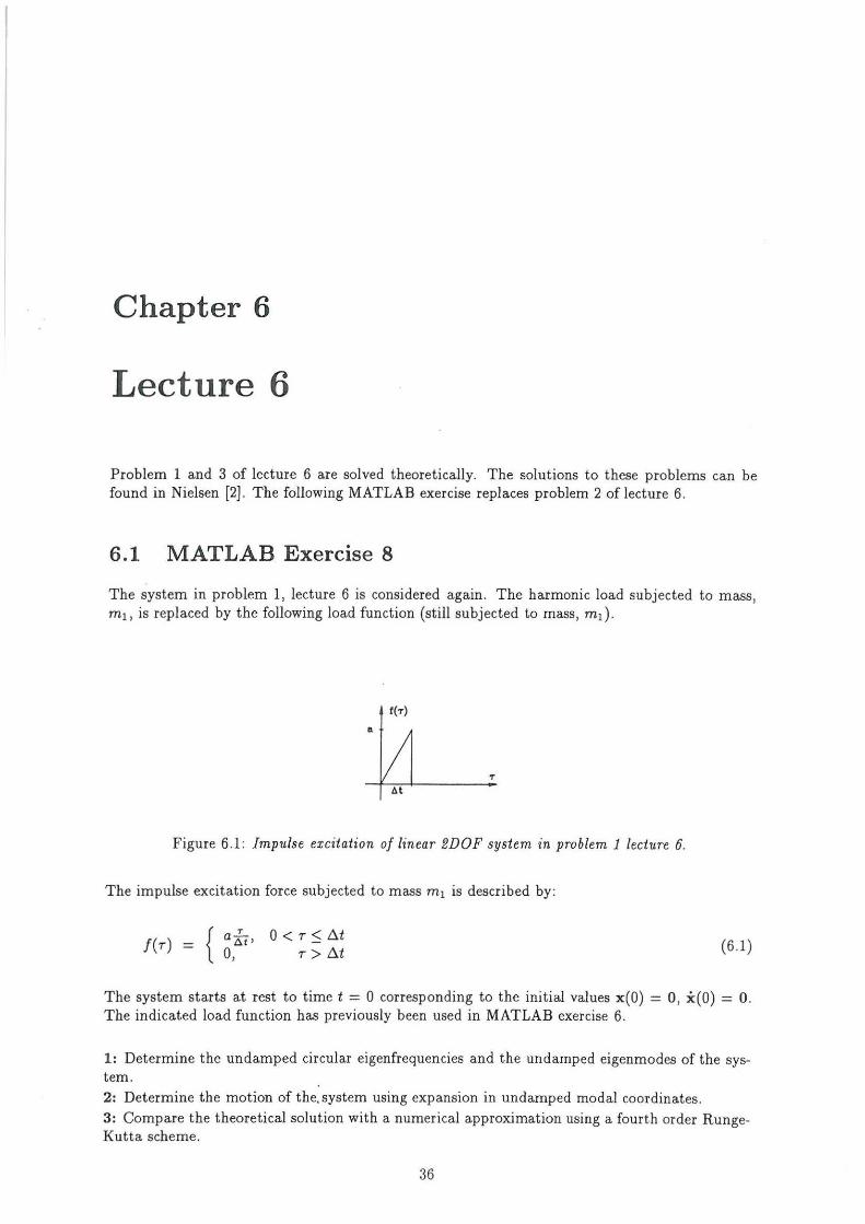
The system in problem 1, lecture 6 is considered again. The harmonic load subjected to mass, m1 , is replaced by the following load function (still subjected to mass, m1).

a

Figure 6.1: Impulse excitation of linear 2DOF system in problem 1 lecture 6.

The impulse excitation force subjected to mass m 1 is described by:

f(r) = { a~t ' O<r~tlt 0, T >At (6.1)

The system starts at rest to time t = 0 corresponding to the initial values x (O) = 0 , :X: (O) = 0. The indicated load function has previously been used in MATLAB exercise 6.

1: Determine the undamped circular eigenfrequencies and the undamped eigenmodes of the system. 2: Determine the motion of the. system using expansion in undamped modal coordinates . 3: Compare the theoretical solution with a numerical approximation using a fourth order RungeKutta scheme.

36



The governing differential equation of the system is:

Mx(t) + Kx(t) = f(t) (6.2)

x = [ ~~ ] , f(t) = [ f~t) ] , M = [ ~1 ~2 ] , K = [ k1_~2k2 ~~2 ] (6 .3)

The frequency condition is used to calculate the undamped circurlar eigenfrequencies and undamped eigenmodes.

(6.4)

Undamped circular eigenfrequencies

]) = 0~

(6.5)

wr } - k,m2+k2(m,+m2)±Jk:m~+k~(m2+m,) 2 +2k,k,m,(m,-m ,) w~ - 2m,m,

Undamped eigenmodes

If <l>~i) = 1 it then follows from the second equation of (6.4) that :

~ (6 .6)

Where the circular eigenfrequencies are given by (6.5).

Motion of system

The motion of the system can be describe by expansion of undamped modal coordinates:

(6 .7)

The undamped eigenmodes of the system are known from (6.6) . The modal coordinates q;(t) are found from (see Nielsen [1], p. 70, (3-166)):

q;(t) = 11

h;(t- r)F;(r)dr (6.8)

Where :

h;(t) { 0 - 1-sin(w·t) t > 0 MtWi t

t < 0 (6 .9)


(6.10)

(6.11)

q:(t) = ~\i) rmin(t,A.t ) Sl.n(w·(t- r))f(~)d~ -~ rmin(t,A.t ) Sl'n(w ·(t- ~))-rd~ • M;w; Jo l ' ' - A.tM;w; Jo l ' ' '

~(i) [ J min(t,A.t ) A.:M· J r cos(wi(t- r)) + l sin(wi(t - r)) ,wi w, 0

(i)

A.~!J;wf(cos(wi(t- min(t, ~t)))min(t , ~t)) + ~; sin(w;(t- min(t, ~t))- sin(w;t))

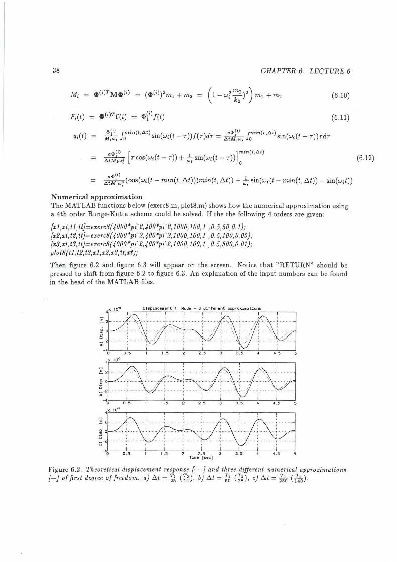
Numerical approximation The MATLAB functions below (exerc8.m, plot8.m) shows how the numerical approximation using a 4th order Runge-Kutta scheme could be solved. If the the following 4 orders are given:

{xi, xt, tl, tt}=exerc8(4000*p{ 2,400*pt 2,1000,100,1 , 0. 5,50, 0.1}; {x2,xt, t2, tt}=exerc8(4000*pi" 2,4 OO*pt 2,1000,100,1 , 0.5,1 00, 0. 05}; {x3,xt, t3, tt}=exerc8(4000*pi" 2,400*p( 2,1000,100,1 , 0.5,500, 0.01}; plot8(t1, t2, t3,x1, x2, x3, tt,xt};

Then figure 6.2 and figure 6.3 will appear on the screen. Notice that "RETURN" should be pressed to shift from figure 6.2 to figure 6.3. An explanation of the input numbers can be found in the head of the MATLAB files .

x 10~ Displacement 1 . Mode - 3 different approximations

!--~~~0~.~5--~1---1~.~5---27-~2~.~5---37-~3~.5~--.~--.~.5~~5

i--~~~0~.~5--~1---1~.~5---27-~2~.~5 ---37-~3~.~5---.~--.~.5~~5

Time [sec)

Figure 6.2: Theoretical displacement response { · -} and three different numerical approximations [-]of first degree of freedom. a) b.t = Ig- (fi), b) D.t = f5- (~),c) ~t = fto (ffo ).

(6.12)


, . . . . . . . . .

t:~ -:u 0.5 I 1.5 2 2.5 3 3.5 ~ ~ . 5 5

~-~··•l•••••••ftd -:u 0.5 I 1.5 2 2.5 3 3 .5 ~ ~ .5 5

!-:~ - 1o~--~o~.~5~--~~----~~~.5~--~2--~~2~.s~--~3~--~3~.~5----~~----~~~.s~~~5

Time [sec]

39

Figure 6.3: Theoretical displacement response { · } and three different numerical approximations [-}of second degree of freedom. a) ~t = ft (H), b) ~t = f& (~), c) ~t = fto (ffo).

6.1.2 MATLAB Files ****************************************************************


Call kl k2 m1 m2 a dta n dt Return xn xt tn tt

File for MATLAB Exercise 8, Lecture 6 EXERC8.M To calculate the response of the 2DOF system described in problem 1, lecture 6. A RungeKutta fourth order method is used. exerc8(kl,k2,m1,m2,a,dta,n,dt) Stifness of first linear spring Stifness of second linear spring Mass 1 Mass 2 Maximal impulse force Time lengt of impulse force Number of points in approximtation Time distance between points (xn,xt ,tn,tt) Displacement response matrix (approximation) Displacement response matrix (Theoretically) Time vector corresponding to xn Time vector corresponding to xa

**************************************************************** function (xn ,xt ,tn,tt]=exerc8(k1,k2,m1,m2,a,dta,n,d t) M(l ,l)=ml ; M(1,2)=0; M(2,1)=0; M(2,2)=m2; K(l,l)=kl+k2; K(1 ,2)=-k2; K(2,1)=-k2; K(2 ,2)=k2; (V ,D]=eig(K,M) Phi2= V( :,1)/V(2,1 ); Phil= V( :,2)/V(2,2); w2= sqrt(D(l,l)); wl=sqrt(D(2,2)); MI= inv(M); tn:=O:dt:n*dt; xn= zeros(2,n+l); dxn= zeros(2,n+ 1); c= -MI*K; for i= l :n, if (tn(i)j= dta) f=(a/dta 0]'; else f= (O 0]'; end;

40

k1 =O.S*dt*( c*xn(1 :2,i)+MI*f*tn(i) ); K=O.S*dt*(dxn(l:2,i)+O.S*kl); k2=0.5*dt *( c*(xn(l :2,i)+K)+MI*f*(tn(i)+dt/2)); k3=0.5*dt *( c*(xn(1 :2,i)+K)+MI*f*(tn(i)+dt/2)); L=dt*( dxn(1:2,i)+k3); k4=0.5*dt* ( c* (xn(1 :2,i )+L )+MI*f*tn(i+ 1)); xn(l :2,i+ 1 )==xn(l :2 ,i)+dt *( dxn(1 :2,i)+(kl +k2+k3) /3); dxn(1:2,i+ 1 )==dxn(1 :2,i) +(l/3)*(kl +2*k2+2*k3+k4); end; length=n*dt; dt=length/2000; tt=O:dt:length; xt=zeros(2,2000); c1=a*Phi1(1)/( dta*wl '2*Phil '*M*Phil ); c2=a*Phi2(1 )/ ( dta*w2'2*Phi2'*M*Phi2); for i=1:2001, tl=min(tt{i) ,dta);


xt(: ,i)=Phi1 *cl*( t1 *cos( wl * ( tt(i)-tl) )+(1 /wl )*(sin{ wl *( tt(i)-tl) )-sin( wl *tt(i) )) ) ; xt(: ,i)=xt( :,i )+Phi2*c2*( t1 *cos( w2*(~t(i)-tl) )+(I/w2)*(sin( w2*( tt(i)-tl) )-sin( w2*tt(i))) ); end; ****************************************************************


Call t1 t2 t3 x1 x2 x3 tt xt Return

File for MATLAB Exercise 8, Lecture 6 PLOT8.M To plot the displacement response for a 2DOF system in MATLAB Exercise 8, lecture 6. Theoretical response versus numerical approx. plot8( tl,t2,t3,x1,x2,x3,tt,xt) Time vector (1. Approximation) Time vector {2. Approximation) Time vector (3. Approximation) Displacement matrix (1. Approximation) Displacement matrix (2. Approximation) Displacement matrix (3. Approximation) Time Vector (Theoretical) Displacement matrix theoretically Graphical plots

**************************************************************** function plot8(tl,t2,t3,xl,x2,x3,tt,xt) clg; subplot(3,1 ,1) ,plot(tl ,xl (1,: ),tt,xt(1,: ) , ': '); ylabel('a) Disp. [m]'); title('Displacement 1. Mode- 3 different approximations') grid; subplot(3,1 ,2) ,plot(t2,x2{1 ,: ),tt,xt(1 ,: ), ':'); ylabel('b) Disp. [m)'); grid; subplot(3,1,3) ,plot(t3,x3(1 ,: ),tt,xt(l,: ), ': '); ylabel('c) Disp. [m]'); grid; xlabel('Time [sec]') pause; clg; subplot(3,1 ,1) ,plot(tl,xl {2,: ),tt,xt(2,: ), ' : '); ylabel('a) Disp. (m)'); title('Displacement 2. Mode- 3 different approximations') grid; subplot(3,1,2) ,plot(t2,x2{2,: ),tt,xt(2,:), ': '); ylabel('b) Disp. [m)'); grid; subplot(3,1 ,3) ,plot( t3,x3(2 ,: ),tt,xt(2,: ), ': '); ylabel('c) Disp. (m]'); grid; xlabel{'Time [sec)') ****************************************************************

Chapter 7

Lecture 7

Problem 1 and 2 of lecture 7 are solved theoretically. The solutions to these problems can be found in Nielsen [2]. Both problems are considered as essential. It is recommended the groups to solve one of the problems in common. The other problem should be solved individually. The individually solved problem is replaced by the following MATLAB exercise. MATLAB exercise 9 is an extension of MATLAB exercise 8.


The system in problem 1 of lecture 6 is considered again. This system is not undamped as in problem 1 of lecture 6. The system and the excitation is shown in figure 7.1 and 7 .2.

I-- Xt 1--Xz

Figure 7.1: Linear viscous damped two degree of freedom system.

f(T)

a

C.t

Figure 7.2: Excitation subjected to mass m 1 .

41


The equations of motion becomes:

Mx(t) + Cx(t) + Kx(t) f(t) ' t>O (7 .1)

x(O) = 0, x(o) = o

Where:

M= [ ~1 (7.2)

The data for the system are:

kt 2 N k2 2 N kg kg - = 4?r -k-m1 = 1000kg - = 4?r -k- m2 = 100kg c1 = 0.04?r- c2 = 0.081r- (7.3) m1 m g m2 m g s s

1: Show, that a theoretically solution by expansion in undamped modal coordinates is impossible. 2: Determine the damped mode shapes <f>Ci) and the characteristic values Aj of the system. (Rewrite to a linear eigenvalue problem of order 4.) 3: Determine the response of the system by expansion in damped modal coordinates and compare the solution with a numerical calculation using a 4th order Runge-Kutta scheme.

7 .1.1 MATLAB Solution

Ad 1) To solve the linear differential equation in (7 .1) by expansion in undamped modal coordinates the following decoubling condition should prevail.

(7.4)

Define the following damping coefficients:

~Ci)c~U) _ { (ij i =1= i 2Jwiwi Mi Mj - ( i i = j

(7.5)

The undamped mode shapes and the eigenfrequencies are determined in problem 1 of lecture 6.

k1m1 + k2(m1 + m2) ± /(kfm~ + k~(mt + m2)2 + 2k1k2m2(m2- mt)) 2m1m2

(7.6)

(7.7)

The damping ratios can be calculated theoretically. Alternatively it is choosen to apply a numerical calculation using a MATLAB function (exerc9a.m) . If the following order are given and the MATLAB function has been implemented the decoubling matrix appears on the screen. An explanation to the input numbers can be found in the head of the MATLAB file .

exerc9a(4 OOO*p( 2,400*pi' 2, 1000,100, 0. 04 *pi, 0.08*pi};

[ (1 (12 ] = 10-3 . [ 0.0770 0.0938 ] (21 (2 0.0938 0.1403 (7.8)

As seen (12 = (21 #- 0, so modal decoupling does not take place . Notice that ( 12 = 0.0938 < v'G(2 = /(0.0770 · 0.1403 · 10-6 ) . This condition must identically be fullfilled for a symmetric


and dissipative damping matrix, see Nielsen (1), p. 72, (3-180). If the theoretically solution by expansion in undamped modal coordinates should be exact, the decoubling condition should be fulfilled . This is not the case for the system. A solution by expansion in undamped modal coordinates can only be approximate.

Ad 2) To calculate the damped mode shapes c})Ci) and the characteristic values )..j the linear differential equations (7.1 ) is rewritten to state variables. This reduces the eigenvalue problem to a linear eigenvalue problem of dimension 4.

Ai + Bz = 0 (7.9)

A=[~~] (7 .10)

The linear eigenvalue problem reduces to:

(>.A+ B)~ = 0 (7.11)

If (7.11) is solved the solutions~ whould have the form:

(7 .12)

If the following order are given and the MATLAB function (exerc9b.m) has been implemented the eigenvalues ).. and the eigenvectors ~ app ears on the screen. An explanation to the input numbers can be found in the head of the MATLAB file. The eigenvectors are normalized to have q>~ ) = 1.

{V, D}=exerc9b{4 OOO*pi" 2,4 OO*pi" 2,1000,100, 0. 04*pi, 0. 08*pi);

Eigenvalues

[ -0.0004 f 5.3678i

Eigenvectors

[

0.2702 + O.OOOli 1.0

-0.0008 + 1.4501i -0.0004 + 5.3678i

0 - 0.0004 - 5.3678i

0 0

0.2702- 0.0001i 1.0

-0.0008- 1.4501i -0.0004- 5.3678i

0 0

-0.0001 + 7.3547i 0

- 0.3702 + 0.0003i 1.0

-0.0015- 2.7224i -0.0010 + 7.3547i

0 J 0 0 (7.13)

- 0.0001 - 7.3547i

-0.3702 - 0.0003i l

-0.00151~ 2.7224i J (7·14

) -0.0010 - 7.3547i

Notice how both the eigenvalues and the eigenvectors turns out in complex conjugate pairs.

Ad 3) Especially the displacement response can be found by:

2

x(t) 2 L R e( c})U)qj (t)) (7.15) j = l


Where Cli(j) are the damped mode shapes and damped modal coordinates are:

>. · t (") ([ ->.·r ]min(t,.6.t) ( ) ) ~<I> ) _e _J_T + 1 fmin t,.6.t ->. T d .6.tmi 1 ->.i o >.i Jo e J T

(7.16)

Where mj is the damped modal mass given by (see Nielsen [1], p. 77, (3-212)).

mj Cli(j)TCC!i(j) + 2>.jcti(j)TMC!i(j)

(7 .17)

The damped mode shapes and the eigenvalues of the system are calculated in the solution to question 2. This means that if the last statement of (7.16) is used in (7.15) an analytical solution to the displacement response of the system is obtained. To compare this theoretical solution with a numerical approximation using a 4th order Runge-Kutta scheme the MATLAB function (exerc9c.m) is used. An explanation of the input numbers can be found in the head of the MATLAB file. If the following order are given figure 7.3 and figure 7.4 will appear on the screen .

m1 = 1 000; m2= 1 00; cl =0. 04 *pi; c2=0. OB*pi; k1 =4 OOO*pt 2; k2=4 OO*pt2; [t1,x1, tt,xt}=exerc9c(V,D, m1, m2, cl, c2,k1, k2,1 00, 0.5,25, 0. 02); [t2,x2, tt,xt}=exerc9c(V,D, m1, m2, cl, c2,k1,k2,1 00, 0.5,50, 0. 01); {t3, x3, tt,xt}=exerc9c(V,D, m1, m2, cl, c2,k1,k2, 100, 0. 5,1000, 0. 0005}; plot9(t1, t2, t3, x1, x2,x3, tt, xt};

7.1 . MATLAB EXERCISE 9 45

!--~~--~0~.~5----~1--~1~.~~----2~--~2~.~5----3~--~3~.75----~ .. ----4~.75--~5

Figure 7.3: Theoretical displacement response [· · ·] and 3 different numerical approximations[-]

f fi t d f f d ) At - I'l._ - ;G_ b) At - I'l._ - ;G_ ) At - .I..J.... - .I.l._ o rs egree o ree om. a u - 12 - 10 u - 24 - 20 , c u - 24o- 2oo·

t_: :; -o · 0 2(; o. 5 1 1 . 5 2 2. 5 3 3 . 5 4 4 . 5 5

0 .02~,.::: ~~-: e : = : : : : : : = ~ 0.01 ........... ; .... ....... : ........... ; ......... _.: ........... ; .. .. .... ··:·"'"'~" ":"'""'"" : ' ' "' "' ' " ':'" ' """

! -0.0 ~ .... . .. .. . :, ... ·. · ::: ·:r · .. ·: :··:.:_ ,· --~ - : _··: ::r>·. · .- __ :.:,: ---:.:::.: : t~.: .. :: ·: :: r·. :::: · ~: :. ,: :.:. :: :· :· ·~·~· :: ·: :: · · :~ --.0 : : : : : : : : :

-o.o::o 0.5 1 1.5 2 2.5 3 3.5 4 4 . 5 5

' ·"' ~ 0.005 " " . . i .... '"'+". "" .i ... " .. : .. . " ... . ; ........ i . "' .i. " "> '" . : .. "' . . . : : : : : : .

5} 0 ··· : ·· . . .. . . ... ·: ........ . . :. ··········:· . ........ ·:· . .... . ... -~· . .... . .. .; .. . .. . . .. .. . . ... .. . .. . · · . ...... .. . . "'1"'4 : : • : : : • : :

;-0.005

-o· 01o 0.5 1 1.5 2 2 .5 3 3.5 4 4.5 . 5 Time [sec]

Figure 7.4: Theoretical displacement response [· · ·] and 3 different numerical approximations[-]

f d d f f d ) At - I'l._ - ;G_ b) At - I'l._ - Ll_ ) At - .I..J.... - .I.l._ o secon egree o ree om. a u - 12 - 10 L.). - 24 - 20 , c u - 240 - 200 -

As seen the numerical solution based on the Runge-Kutta scheme requires very small time steps


before converging is achieved. A typical time step of D.t = fto should be compared with a time step of D.t = ~ of a SDOF system. As n (number of DOF) is further increased the time step is even further reduced. Hence the Runge-Kutta scheme becomes increasingly ineffective at large values of n, and should be rep laced by other integration schemes.

7.1.2 MATLAB Files ****************************************************************

MATLAB Function Purpose Call

.. kl k2 ml m 2 cl c2 Return

File for MATLAB Exercise 9, lecture 7 EXERC9A.M To calculate the decoubling matrix exerc9a(kl,k2 ,ml ,m2,cl ,c2) Stifness of linear spring 1 stifness of linear spring 2 Mass of mass 1 Mass of mass 2 Damping constant 1 Damping constant 2 Damping ratio matrix

**************************************************************** function exerc9a(kl ,k2,ml ,m2 ,cl ,c2) konst=sqrt(k1"2*m2"2+k2"2*(ml+m2r2+2*kl *k2*m2*(m2-ml)) ; wl =(kl *m2+k2*(ml+m2)-konst)/(2*ml *m2); w2=(kl *m2+k2*(ml+m2)+konst)/(2*ml *m2); wl =sqrt(wl) ; w2=sqrt(w2) ; M(l,l)=ml ; M(l ,2)=0; M(2,1)=0; M(2,2)=m2; Phil=[l-w1"2*m2/k2 1] '; P hi2=[1-w2"2*m2/k2 1]'; C(l,l)= c l+c2; C(l ,2)=-c2; C(2 ,1)=-c2; C(2,2)=c2; decou(l ,l)= Phil '*C*Phil; decou(l ,2)= Phil '*C*Phi2; decou(2 ,1) = Phi2'*C*Phil ; decou(2,2) = Phi2 '*C*Phi2 ; mml=Phil'*M*Phil; mm2= Phi2'*M*Phi2; zll=decou(l,l) /(2*wl *mml); z12=decou(l ,2) / (2*sqrt(wl *w2*mml *mm2)) ; z2l= decou(2,1)/(2*sqrt(wl *w2*mml *mm2)); z22=decou(2,2)/(2*w2*mm2); damp( :, l)=[zll z21] '; damp(: ,2)=[z12 z22]'; dampingratios=damp ****************************************************************


Call kl k2 ml m2 cl c2 R eturn V D

File for MATLAB Exercise 9, lecture 7. EXERC9B.M To calculate the eigenvalues and eigenvectors of linear state variable eigenvalue problem. exerc9b(kl ,k2,ml ,m2,cl ,c2) Stifness of linear spring 1 stifness of linear spring 2 Mass of mass 1 Mass of m ass 2 Damping constant 1 Damping constant 2 Eigenvalues and eigenvectors Normalized eigenvectors Eigenvalues

**************************************************************** function [V ,D]=exerc9b(kl ,k2,ml ,m2,cl ,c2) M(l ,l) = ml; M(1 ,2)=0; M(2,1)= 0; M(2,2)= m2; C(l ,l )= c l +c2; C(1,2)= -c2; C(2,1) = -c2; C(2,2)= c2; K(l,l)= kl+k2; K(1 ,2)= -k 2; K(2,1) = -k2; K(2,2) = k2; 0 =zeros (2,2) ;


Al=[C M]'; A2=(M 0]'; A=[Al A2]; Bl= [K 0]'; 82=(0 -M]'; B=[Bl B2]; [V ,D]=eig(B,-A); V( :,l)=V( :,1 )/V(2,1); V(:,2)= V( :,2)/V(2,2); V(:,3)=V( :,3)/V(2,3); V( :,4)= V( :,4)/V(2,4); eigenv<;Uues=D Eigenvectors= V ****************************************************************


Call V D ml m2 cl c2 a dta n dt Return tn xn tt xt

File for MATLAB Exercise 9, lecture 7. EXERC9C.M To calculate the displacement response of the system. Both the theoretical solution and a numerical solution using a 4th order RungeKutta scheme is used. exerc9c(V ,D ,ml ,m2 ,cl ,c2,kl ,k2 ,a ,dta,n ,dt) Normalized complex mode shape vectors Complex eigenvalues Mass of mass 1 Mass of mass 2 Damping constant 1 Damping constant 2 Maximal excitation Duration of excitation Number of points in approximation Time distance between approximations

Time vector for numerical approximation Numerical approx. matrix for displacement T ime vect or for theoretical solution Displacement matrix for theoretical solution

**************************************************************** function [tn,xn,tt ,xt)=exerc9c(V ,D ,ml ,m2,cl ,c2,kl ,k2 ,a,dta,n ,dt) Phil=V(l:2,2) ; Phi2=V(l :2,1) ; Ll=D(2,2); L2=D(1 ,1 ); M(l ,l )=ml; M(1 ,2)=0; M(2,1)=0; M(2,2)=m2; C(l ,1 )=cl+c2; C(l ,2)=-c2; C(2 ,1 )=-c2; C(2,2)=c2; K(l ,l) = kHk2; K(1,2)=-k2; K(2,1)=-k2; K(2 ,2) = k2; MI=inv(M) ; F= [a/dta 0]'; tn=O:dt :n*dt; xn=zeros(2,n+l); dxn=zeros(2,n+l) ; for i=l :n, if (tn(i)i=dta), Fl=F; else Fl=[O 0]'; end; kl = O.S"dt * ( -MI*C*dxn(: ,i )-MI*K*xn( :,i) +MI*Fl *tn(i)) ; KK= O.S*dt*(dxn(:,i)+O.S*kl) ; k2=0.5"dt *( -MI*C*( dxn( :,i)+kl )-MI*K*(xn(: ,i)+KK)+MI*Fl *( tn(i)+O.S*dt)); k3= 0.S*dt*(-MI"C"( dxn(: ,i)+k2)-MI"K*(xn( :,i)+KK)+MI*Fl *( tn(i)+O.S"dt )); LL=dt *( dxn( :,i)+k3); k4=0.5*dt *( -MI*C*( dxn( :,i)+2*k3)-MI"K*(xn( : ,i)+LL )+MI*Fl *( tn(i)+dt) ); xn(: ,i+ 1 )=xn( :,i)+dt *( dxn( :,i)+(l / 3)*(kl +k2+ k3) ); dxn( :,i+ 1 )= dxn( :,i)+(l / 3)*(kH2*k2+2*k3+k4) ; end; mdl= ( cl + c2) *Phi1 (1 P-2*c2"Phil (1 )+c2+2"Ll *(Phil (1 P*m1 + m2); md2= (cl +c2)*Phi2(1 P-2*c2*Phi2(1 )+ c2+2*L2* (Phi2(1 P*ml +m2) ; Cl=a*Phil (1) / ( d ta*md1 *Ll); 02=a *Phi2(1 )/ ( dta*md2*L2) ; dtt=n*dt / 1000; tt=O:dtt:n*dt; xt=zeros(2,1001); for i= l :lOOl, t = min(tt(i) ,dta) ; ql=-Cl *exp(Ll *tt(i) )*( exp( -Ll *t )*t+(l/Ll )*( exp(-Ll *t )-1)); q2= -C2*exp(L2*tt(j) )*( exp( -L2*t )*t+(l/L2)*( exp( -L2*t)-l)); xt(: ,i)=2*(real(Phil*ql )+real(Phi2*q2) ); end; ****************************************************************

47

48

**************************************************************** MAT LAB FUnction Purpose

Call t1 t2 t3 x1 x2 x3 tt xt Retum

File for MATLAB Exercise 9, Lecture 7 PLOT9.M To plot the displacement response for a 2DOF system in MATLAB Exercise 9, lecture 7. Theoretical response versus numerical approx. plot9( t1 ,t2,t3,x1,x2,x3,tt,xt) Time vector (1. Approximation) Time vector (2. Approximation) Time vector (3. Approximation) Displacement matrix (1. Approximation) Displacement matrix (2. Approximation) Displacement matrix (3. Approximation) Time Vector (Theoretical) Displacement matrix theoretically Graphical plots

**************************************************************** function plot9(tl ,t2,t3,x1 ,x2,x3,tt,xt) clg; subplot(3,1 ,1) ,plot(tl ,x1 (1 ,: ) ,tt,xt(1,:), ': '); ylabel('a) Disp. (m]'); title('Displacement 1. Mode- 3 different approximations') grid; subplot(3,1 ,2),plot(t2,x2(1,: ),tt,xt(l,: ), ': '); ylabel('b) Disp. (m)'); grid; subplot(3, 1 ,3) ,plot(t3,x3(1 ,: ),tt,xt(l, : ), ': '); ylabel('c) Disp. (m)'); grid; xlabel('Time (sec)') pause; clg; subplot(3,1, 1) ,plot(tl ,xl (2 ,: ), t t,xt(2,: ) , ': ') ; ylabel('a) Disp. (m)'); title('Displacement 1. Mode- 3 different approximations') grid; subplot(3,1 ,2) ,plot( t2,x2(2,: ),tt ,xt(2, : ), ': '); ylabel('b) Disp. (m)'); grid; subplot(3,1 ,3) ,plot(t3,x3(2,: ),tt,xt(2,:) , ': '); ylabel('c) Disp. (m)'); grid; xlabel( 'Time (sec)') ****************************************************************


Chapter 8

Lecture 8

Problem 3 of lecture 8 is solved theoretically. Problem 1 and 2 of lecture 8 are solved individually. The solutions to these problems can be found in Nielsen [1]. The following MATLAB exercises replaces the problems, which are solved individually. MATLAB exercise 10 is an extension of MATLAB exercise 8 and 9.


The systems in MATLAB exercise 8 and 9 are considered again .

1) Compare the theoretical solution of the system in MATLAB exercise 8 with a solution, where only 1 undamped modal coordinat is used (system reduction) .

2) Compare the theoretical solution of the system in MATLAB exercise 9 with a solution, where only 1 damped modal coordinat is used (system reduction).


If the second mode can be considered as not being dynamically excited, then only the quasi-static response of this mode is taken into account.

Ad 1) The response of the unda.mped two degree of freedom system in MATLAB exercise 8 using system reduction is:

x(t) = q1 (t)~(l) + (K- 1 - -2-1 -~(l)~(l)T) f(t) wlMl

If the quasi-static response is ignored the response becomes:

(8.1)

(8.2)

The loading f(t) is caused by a triangular impulse of duration Llt = ~T1 on the first mass. Hence fort > Llt f(t) = 0 and (8.1) and (8.2) coincide. The discontinuity of (8.1) at the tune t = Llt is caused by the discontinuity of the quasi-static part of the response due to the jump of the impulse. None of the approximations are good since the 2nd mode is excited significantly. The theoretically solution by expansion in undamped modal coordinates is known from MATLAB exercise 8. This solution and the approximation given by (8.1) are implemented in the MATLAB function below (exerclOa.m). If the following order are given.

49


exercl Oa(4 OOO*pi" 2,4 OO*pt 2,1000,100, 1, 0.5, 100, 0. 05);

Then figure 8.1 will appear on the screen.

. .

~-1 . . .. . . . . . .. [ .. . .. .... \ . .: . . .. . / . .. i ....... .. ... L. ... .. :-: ... ~ c; ~ : : : ~ . . .

-2 .. ' . . . . . ··! ...... ..... :~·. ·. ·.· ·: ' .. , ... : .... .. ... .

Figure 8.1: Response calculated from system reduction (8.1} [-], system reduction without quasistatic response [---}, theoretically solution {-}.

Ad 2) The response of the damped two degree of freedom system in MATLAB exercise 9 using system reduction is:

(8.3)

If the quasi-static response is ignored the response becomes:

(8.4)

The theoretically solution by expansion in undamped modal coordinates is known from MATLAB exercise 9. This solution and the approximation given by (8 .2) are implemented in the MATLAB function below (exerclOb.m). If the following order are given.

exercl Ob(1 000,100, 0. 04 *pi, 0.08*pi,4 OOO*pt 2,400*piA 2, 1, 0.5, 100, 0. 05);

Then figure 8.2 will appear on the screen.


<! ..

" "8 E

I ...... .

" "8 E 0.5

N

~ 0 _r,;,, ,:

.... 0

-0. 5

. .. . :·~-:. ~ ...... ''> .. ·:·. :

.. \ .. ~~···

.,

51

... ... .......... . .. ·········:······· ·· ..

;···. :.··· ··········:·:-·····:··· ·······,:-:; .. : ........ .

Figure 8 .2: Response calculated from system reduction (8.3} [- }, system reduction without quasistattc correctzon (8.4} [- --}, theoretically solution{-}.

8.1.2 MATLAB Files ****************************************************************

MATLAB Function P urpose

Call k1 k2 m l m2 a dta n

dt Return

File for MATLAB Exercise 10, Lecture 8 EXERClOa.M To calculate the response of the 2DOF system described in problem 1, lecture 6. The response is calculated using expansion in undamped modal coordinats and a approximation using system reduction. exerc 10a{kl ,k2 ,ml,m2 ,a,dta,n,d t) Stifness of first linear spring Stifness of second linear spring Mass 1 Mass 2 Maximal impulse force Time lengt of impulse force Number of points in response calculation Time distance between points Graphical plot - Comparison

**************************************************************** function exerc10a{kl,k2 ,ml,m2,a,dta,n ,dt) M{ 1,l)=ml; M(1,2)=0; M(2,1)=0; M(2,2)=m2; K{l,l )=kl+k2; K{1 ,2)=-k2; K{2 ,1)=-k2; K{2,2)=k2; [V,D]=eig{K,M); Phi2=V(:, l)/V(2,1); Phil=V(: ,2) /V(2,2); w2=sqrt{D(l,1) ); wl =sqrt(D{2,2) ); MI=inv{M); KI=inv(K);

t=O:dt:n*dt; xt=zeros{2,length{ t)); cl=a*Phi1{1)/(dta*w1 -2*Phil'*M*Phi1 ; c2=a*Phi2(1 )/ ( dta*w2-2*Phi2'*M*Phi2;

52

for i=l:length(t) , tl=min(t(i) ,dta) ; xt(: ,i)=Phil *cl*( t1 *cos( wl *( t(i)-tl ))+(1 /wl )*(sin( wl *( t(i)-tl) )-sin( w1 *t(i))));


xt(: ,i)=xt(: ,i)+Phi2*c2*( tl *cos( w2*(t(i)-tl) )+(1/w2)*(sin(w2*( t(i)-t1) )-sin(w2*t(i)) )) ; end;

x=zeros(2,length( t )); c3=Phil *Phil'/ (wl.2*(Phil'*M*Phil)); f=[a/dta 0] '; for i= 1 :length( t), t1= min(t(i),dta); if t(i)j=dta, fl = f; else fl= [O 0]'; end; x(: ,i)= Phil *cl *(tl *cos(wl *(t(i)-t1) )+(1/wl )*(sin( w1 *( t(i)-tl) )-sin( wl *t(i) )) ) ; xl{:,i)=x(:,i); x( :,i)=x(:,i)+(KI-c3)*fl *t(i); end;

clg; subplot{211 ),plot( t,xt(l,: ),':',t,x(l,:) ,t ,xl {1 ,: ),'- '); ylabel('Disp. 1. m ode'); grid; subplot ( 212) ,plot( t,xt (2,:) ,': ',t ,x{2,:) ,t ,x1 {2,:) ,'-'); ylabel( 'Disp . 2. mode'); xlabel('Time (sec]'); grid; ****************************************************************

****************~*********************************************** MATLAB Function Purpose

Call ml m2 cl c2 k1 k2 a dta n dt Return

File for MATLAB Exercise 10, lecture 8 EXERClOB.M To calculate the displacement response of the system. Both the theoretical solution and a approximate solution using system reduction is made exercl0b(ml,m2,c1,c2,kl ,k2 ,a.,dta,n ,dt) Mass of mass 1 Mass of mass 2 Damping constant 1 Damping constant 2 Stifness constant 1 Stifness constant 2 Maximal excitation Duration of exci tation Number of points in approximation Time distance b etween approximations Graphical plot - Comparison

**************************************************************** function exerc10b{ml,m2,cl,c2,k1,k2,a,dta,n,dt) M(l,l )=ml ; M(1,2)=0; M{2,1)=0; M(2,2)= m2; C{1 ,1)=cl+c2; C(1 ,2) =-c2; C(2,1)=-c2; C{2 ,2}=c2; K(l ,l )=ki+k2; K(l ,2}=-k2; K(2 ,1)=-k2; K(2,2}=k2 ; 0=zeros(2,2}; A=(C M; M 0) ; B=(K 0; 0 -M) ; (V,D]=eig(B,-A); V( :,l)=V( :,1 )/V(2,1}; V( :,2)= V(:,2)/V(2,2); V( :,3)=V( :,3)/V(2,3}; V( :,4)= V(: ,4)/V( 4,2); Phil=V(1:2,2); Phi2= V( 1:2,1); Ll = D(2,2) ; L2= D( l ,l) ; MI= inv(M); KI= inv(K) ; F = (a/dta 0)'; mdl = ( c1+c2)*Phil(l}"2-2*cl *Phil (l)+c2+2*Ll *(Phil (1}'2*m1+m2) ; md2= ( cl +c2)*Phi2(1 t2-2*c1 *Phi2!J )+c2+2*L2*(Phi2(1 r2*ml +m2) ; Cl = a *Phil (1 ) / ( dta*m dl *Ll) ; C2= a*Phi2(1 )/ ( dta*md2*L2) ; t = O:dt:n*dt ; xt=zeros(2,length(t)); for i= l :length(t) ,


tl=min(t(i) ,dta) ; ql =-Cl *exp(L1 *t(i))*( exp( -Ll *tl )*tl+ (1 /Ll )*( exp( -Ll *tl)-1 )); q2=-C2*exp(L2*t(i) )*( exp( -L2*t 1) *tl +( 1 /L2) * ( exp( -L2*t1 )-1)); xt( :,i)=2*(real(Phil *ql )+real(Phi2*q2) ); end; for i=l:length(t), tl=min(t(i),dta); if (t(i)i=dta), f=F; else f=(O 0]'; end; q1=-Cl *exp(L1 *t(i))*( exp( -Ll *tl )*tl+(l/L1)*( exp( -Ll *tl )-1 )); x( :,i)=2*real(q1 *Phi1); x1 (: ,i )=x(: ,i); x( :,i)=x(: ,i)+ (KI-2*real((l /{md1 *L1) )*(Phi1 *Phi1 ')) )*f*t(i); end; clg; subplot(2,1 , l ),plot(t,x( l ,:) ,t,xt(l ,: ), ': ',t,xl(l ,: ) , '-'); ylabel{'Disp. 1. mode'); grid; subplot(2,1 ,2) ,plot(t,x(2,:) ,t,xt{2,: ), ':' ,t,x1(2,:), '- '); ylabel('Disp. 2. mode'); xlabel('Time (sec]'); grid; ****************************************************************

53

Chapter 9

Lecture 9

Problem 1 and 2 of lecture 10 is solved theoretically. The solution to these problems can be found in Nielsen [2]. The following MATLAB exercise replaces the problems which are solved individually.


Consider a continous Bernoilli-Euler beam. The beam is simply supported at both end sections A and B and loaded as shown in figure 9 .1.

1(x,t)=10 cos(r.>t)

A B

El,J.'

Figure 9.1: Harmonic loaded continous Bernoulli-Euler beam.

The beam is excited by the dynamic force per unit length f(x , t) = f o cos(wt). The beam is undamped and the following data are valid:

l = 1m , El = 1Nm2, J-1. = (9.1)

The initial conditions at timet = 0 are:

y(x, 0) = 0 , y(x , 0) = 0 (9.2)

Question: Find the stationary motion of the beam. Animate the motion and try to change the frequency of the harmonic load with values in the vicinity of the 3 lowest natural frequencies of the beam.

54



The force-balance differential equation of the system is, see Nielsen [1) , p . 100, (4-9).

84 y(x, t) 82 y(x, t) f ( ) 8x4 + J." 8t2 = o cos wt (9.3)

Because the beam is simply supported as shown in figure 9.1 the boundary condition needed to solve (9 .3) are:

y(O, t) ::: 0 , y(l, t) ::: 0 , ()2y(O , t) = 0

ox 2 - ' (9 .4)

In the present case a solution to the stationary displacement field can be obtained on closed form by direct integration of the partial differential equation for the beam element . The alternative is to use expansion in undamped modal coordiantes (series solution) . The calculations can be found in Nielsen (2], p. 212 ff. The calcutions are omitted here. The solution is:

y(x, t) = U(x) · cos(wt)

Where:

U(x) = 2~ j }J ( -2 + c~i~(1; ) ) si~ (-'f)+ cos (-'f) +

( 1 ~i~~sN;)) sinh ( ,\ y) +cosh (Ay))

pw2[4 ,\4 =

El The natural frequencies of the beam is given by, Nielsen [1], p. 111, ( 4-45):

i 27r2 (ii Wi = TV---;; ' i = 1, 2, 3, ...

Inserting the data from (9 .1) in (9.8) yields: ·2

Wi = Z · 7r , i=1,2,3, ...

(9 .5)

(9.6)

(9.7)

(9 .8)

(9.9)

If the following order are given and the MATLAB function (exercll .m) are implemented , the animation of the stationary motion of the beam will appear on the screen. Because of the limiting speed of the hardware the motion of the beam is animated in slow motion.

exercll (?,1,1 O,pt 2, 1,1};

9.1.2 MATLAB Files ****************************************************************


Call w fO n mu la en EI Return

File for MATLAB Exercise 11 , Lecture 9 EXERCll.M To animate the response of a. simply supported Bemoulli-Euler beam load by a harmonic force. The beam is undamped and the solution is obtained in close form. exercll( w ,fO ,t,mu,laen,EI) Frequency of the harmonic force Amplitude of harmonic force Number of load cycles to animate Mass per unit length of beam Length of beam Material constants of beam Graphical plots - Animation

56

**************************************************************** function [y]=exercll (w,fO,n,mu,laen,EI); f=w/(2*pi); dt=l/(20*f); y( 41 ,20)=zeros; dl=laen/ 40; L=sqrt( sqrt(mu*w-2*laen ·4/EI)); Cl=(l-cos(L) )/sin{L); 02=(1-cosh{L))/sinh(L); C3=f0/(2*w-2*mu); CS =dl *L flaen; for i=l:20, t=(i-l)*dt; C4=C3*cos{w*t); for j=l:41, l=(j-l)*CS; y(j ,i )=04 * {-2 +Cl *sin(l)+cos(l)+C2*sinh(l)+cosh(!)); end; end; ymax=max{max(y)); ymin= min{min(y)); xmax=laen+O.l *laen; xmin=-0.1 *laen; ymax=2*ymax; ymin=2*ymin; for i=1:41, x{i)=(i-l)*dl; end; for j=l:n, for i=l:20, plot(x,y(:,i)); axis{[xmin xmax ymin ymax]); title('Animation of stationary response'); xlabel('Length of beam'); ylabel('Response of beam'); pause(O.S) ; end; end; ****************************************************************


Chapter 10

Lecture 11

Problem 1 June 16, 1989 are solved theoretically. The solutions to the problem can be found in Nielsen (2] . The following MATLAB exercise should also be calculated.


Consider a continuous 2-storey frame structure . The structure is shown in figure 10.1

It. i-'1

3m

3m

5m

Figure 10. 1: 2-st orey frame structure.

The following data is valid for the stifness and mass of the frame structure.

El = 2.0 . 1011 N, . m E2 = E1 E3 = E1

h = 1.945 · 10-5m 4 h = 3.89 · 10-5m 4 13 = 2.63 · 1Q- 5m4 (10 .1)

JJ.l = 1000~ JJ.2 = 2000~ IJ.3 = 46~ Question: Determine the undamped eigenfrequencies and eigen modes for the following number of system nodes, 6,12 ,24.

57


The theoretical solution for the 4 lowest eigenfrequencies are:

h = 1.05Hz, h = 4.31Hz, h = 6.19Hz !4 = 7.17Hz (10.2)


The following orders calculates and plots the eigenfrequencies and the mode shapes ofthe structure when 6,12 and 24 degrees of freedom are used. 6 Node approximation. exerc12a F=[l.0281 4.21 25 8.2186 11 .3539] plot12a{X, T,Shape)

1 . mode shape

'r --.------------lr---<)< I I I

I I

~-~---------~

Figure 10 .2: 6 Node approximation, 1. mode. o node points, *mode shape points, [-- -} undeformed structure, [-] deformed structure.

2 , mode ~hape

Figure 10 .3: 6 Node approximation, 2. mode. o node points, * mode shape points, [-- -] undeformed structure, [-] deformed structure.


3 . mode ~.hape

Figure 10.4: 6 Node approximation, 3. mode. o node points, *mode shape points, [-- -} undeformed stru cture, [- } deformed stru cture.

4 . mode $hape

Figure 10.5: 6 Node approximation, 4. mode. o node points, *mode shape points, [- - -} undeformed structure, [- }deformed stru cture .

12 Node approximation exerc12b F=(1.0281 4.2120 6.1251 7.1140] plot12b(X, T ,Shape)

60

1 . mode shape

~-~--------~~~--------~~

' I Ill ~

I I

'

~~----------~~--------~~


Figure 10 .6: 12 Node approximation, 1. mode. o node points, *mode shape points, [-- -} undeformed structure, [- ]deformed structure.

2. mode shape

I I

~~----------~.-----------~

I I

~

I I I I I I I

~

Figure 10.7: 12 Node approximation, 2. mode. o node points, *mode shape points, [- - -} undeformed structure, [-} deformed structure.


3 . mode shape

Figure 10 .8: 12 Node approximation, 3. mode. o node points, *mode shape points, [-- -] undeformed structure, [-]deformed structure.

4 . mode shape

Figure 10.9: 12 Node approximation, 4. mode. o node points, * mode shape points, [-- -] undeform ed structure, [-] deformed structure.

24 Node approximation exerc12c F=[l.0281 4.2116 6.0751 7.0395] plot12c(X, T,Shape)

62

1 . mode shape

~.---~.---~~--~~--~~~

I 1 I 1

~ ~ I I I 1 ~ ~ I I I I I 1

~ ~ I 1 I 1 I 1

~~---4.---~~--~~--~~1 I I I I

~ ~ I I I 1

+ I

~

~ I I

~ l


Figure 10.10: 24 Node approximation, 1. mode. undeformed structure, [- }deformed structure.

o node points, * mode shape points, [- - -}

2 . mode shape

I I I

~ I I I I I I ~ ~ I I I I ~ '

Figure 10.11: 24 Node approximation, 2. mode. o node points, * mode shape points, [- - -} undeformed structure, [-} deformed structure.

10.1 . MATLAB EXERCISE 12 63

3 . mode shape

Figure 10.12: 24 Node approximation, 3. mode. o node points, * mode shape points, [-- -} undeformed structure, [-} deformed stru cture.

4 . mode :shape

Figure 10.13: 24 Node approximation, 4. mode. o node points, * mode shape points, [-- -} undeformed structure, [-} deformed structure.

The theoretical and the approximative eigenfrequencies of the frame structure are shown in tabel 10.1.

Theory 6 Nodes 12 Nodes 24 Nodes

h 1.05 1.03 1.03 1.03 h 4.31 4.21 4.21 4 .21 h 6.19 8.22 6.13 6.08 f4 7.17 11.35 7.11 7.04

Table 10.1: Eigenfrequencies

10.1.2 MATLAB Files

All MATLAB fil es omitted.

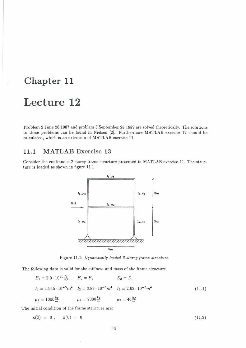
Chapter 11

Lecture 12

Problem 2 June 26 1987 and problem 3 September 28 1989 are solved theoretically. The solutions to these problems can be found in Nielsen (2]. Furthermore MATLAB exercise 12 should be calculated, which is an extension of MATLAB exercise 11.


Consider the continuous 2-storey frame structure presented in MATLAB exercise 11. The structure is loaded as shown in figure 11.1.

3m

t(l)

3m

5m

Figure 11 .1: Dynamically loaded 2-storey frame structure.

The following data is valid for the stiffness and mass of the frame structure.

(11.1)

J.l2 == 2000~ J.l3 = 46~

The initial condition of the frame structure are:

x(O) = 0 , x(O) = o (11.2)

64


In figure 11.2 the impulse load on the frame structure is shown.

t('T)

a

'T

Figure 11.2: Impulse load on 2-storey frame structure

f(r) = { ai.t' O<r:Stlt 0, T > /:lt (11.3)

Where a is a positive constant. Question: Determine the time-varying ·horisontal displacement of the stories and the moment in the upper column at the node, where the load is applied. Use 4 modal coordinates in the approximation. The mode shapes, eigenfrequencies, mass matrix and stifness matrix are known from MATLAB excercise 11 using the case with 24 systems nodes. In the approximation the quasi-static term of higher order modes are ignored. The damping matrix of the structure can be considered to decouple in a expansion in terms of undamped modal coordinates. The damping ratios of the first 4 modes and the constants describing the impulse load are:

(1 = 0.01 ' (2 = 0.005 ' (3 = 0.007 ' (4 = 0.006

a = 100, tlt = 0.2s .


(11.4)

(11 .5)

To calculate the time-varying moment at the excitation point the beam element connecting the node at the excitation point and the node right above is considered. Using standard FE-theory the end section shear forces P1 , P3 and the end-section moments P2, P4 can be cakulated from the conjugated nodal displacement u1, u3 and nodal rotations u 2 , u 4 as follows

-12 -6/ 12

-6/

6/ ] [ U1 ] 2/2 u -6/ u~ 4/2

U4

The signs of the quantities has been depicted on figure 1.3.

~--•- X

P2U2 r-----------------------7

Figure 11 .3: Sign of displacements and forces.

(11.6)

66 CHAPTER 11 . LECTURE 12

The displacement at any node point, j, of the discretized structure can be calculated from the following truncated modal expansion, see Nielsen [1], p. 86, (3-249):

(11.7)

Where j denotes the number of degree of freedom of the excitation point . The differential placement of the modal coordinates are given by the following second order differential equation .

.. 2~' . 2 q; + ..,;w;q; + w; q;

With the initial conditions:

q;(O) = 0 , q;(O) = 0

1 -FM; '

The modal masses and the modal excitation are calculated from:

(11.8)

(11.9)

(11.10)

(11.11)

The solution to an equivalent differential equation to (11.8) is known from MATLAB exercise 4 and appendix A.

<ll<i )a [min(t ~t) ] q;(t) = ~~wf M: + h(t- min(t, ~t))- h(t) + 2(;w;(H(t- min(t , 6-t))- H(t)) (11.12)

Where:

h(t) (11 .13)

(11.14)

The following steps are performed to obtain the solution to the question.

1) Calculate the global mass matrix M, the global stiffness matrix K , the eigenfrequencies w; and the mode shapes <Jl(i).

2) Calculate the modal mass M; and the modal excitation F; from (11.10) and (11.11).

3) Solve (11.8) for the four lowest modes to determine the modal coordinates.

4) Use (11.7) to calculate the displacement response of the excitation point.

5) Use (11.6) to calculate the time-varying moment of the excitation point.

Ad 1) By giving the following orders, equivalent to MATLAB excercise 11, the mass matrix, stifness matrix. eigenfrequencies and mode shapes will be calculated and available in the memory afterwards.

exerc12c

The variables are denoted M,K,F and Shape.


Ad 2) The modal masses and the modal excitations are calc~lated m the MATLAB file exercl3a.m. Give the following order.

[Mi Fi Shapes}=exerc13a(M,Shape)

Ad 3,4,5 Each of the three steps are performed in the MATLAB file exerc13b.m. Give the following order, and the graphs will be shown on the screen. Press enter to continue. The inputs are described in the head of the MATLAB file .

exerc13b{Mi,Fi,Shapes,F,100,0.2,2, 0. 01};

Excitation node

Node above excitation

Figure 11.4: Horizontal displacement response of the storeys. The upper graph shows the upper storey and the lower graph shows the lower storey.

68

11.1.2


Moment i n excitation point 800'r----,-----.----.-----~~~r---~~---r----,-----r----,

600 .......... .; ..

400 ...... .. ..... ......... .

200 .... .. .... , .......... .

- 600

. . ...... ....•............ ; ............ ; ... . . . . ··:····· .. ·····:·········· . .

- I OO%L----0~.-2--~0~.4~~0~.~6--~0~.8-----~L---~1~.2~--~~~.4~--~~-~6--~1~.8~--~2 Time

Figure 11.5: Time-varying moment at the excitation points.

MATLAB Files

All MATLAB files omitted.

Appendix A

Lecture 4

Consider the linear single degree of freedom system in problem 1, lecture 3 Nielsen [2). Instead of a harmonic excitation force the system is excited by an impulse force . The impulse force is shown in figure A .1.

t("T)

a

b.t

Figure A.l: Impulse excitation of the system in problem 1, lecture 3 Nielsen {2].

Determine the solution, x(t), to the linear vibration problem of the system:

i(t) + 2(wox(t) + w5x(t) = f(t) , t > 0 x(t = 0) = 0 , x(t = 0) = 0

(A.l)

Where ( is the damping ratio and w0 is the natural eigenfrequency. The impulse force on the system (see figure A.l) is described by:

f (r) = { a lt, 0 < r :S Llt 0, T > ilt (A.2)

The maximum impulse excitation is a and Llt is the duration of the impulse force.

Analytical Solution

Because the initial conditions of the system are zero (see (A.l)) the displacement response is given by Duhamel's integral (see Nielsen [1], p. 29, (2.131)):

1

t 1 min(t,6t) T

x(t) = 0

h(t- r)f( r)dr = 0

h(t- r)a Llt dr (A.3)

69

70 APPENDIX A. LECTURE 4

The impulse response function , h(t ) is given by (see Nielsen (1], p. 27 (2.119)):

{

- 1-e-(wot sin(wdt) t > 0 h(t) = mwd -

0 t < 0 (A.4)

Where m is the mass of the oscillator and Wd = woJI-=(2 is the damped natural eigenfrequency. The integral in (A.3) is evaluated by partial integration.

x(t) - [H(t- r)f(r)]~ + J; H(t- r )f'(r)dr

-H(O)f(t) + H(t)f(O) + f0min(t,At) H (t - r ) ;,_t dr

;,_t fomin(t ,At) H(t- r)dr

Where H(t ) is the integral of h(t) defined as:

H(t) = i t h(r)dr ~ H(O) = 0

(A.5)

(A.6)

In the last statement of (A.5) it has been used that H(O) = f(O) = 0, f'(r) = ;,_,, r :S tlt and f'(r) = 0, r > 6.t.

In order to evaluate the integral (A .6) the following initial value problem for h(t) is used (see Nielsen [1], p. 27, (2 .119)).

h(r)+2(woh(r)+wfih(r) = 0 , r>O h(O) = 0 I h(O ) = !

Upon integrating (A.7) an expression for H(t) as a function of h(t) is obtained.

[h(r)]~ + 2(w0 [h(r)n + w~[H(r)]~ = 0

Inserting the initial conditions (A.7) provides:

H(t) = _2._ (_.!_- h(t)- 2(woh(t)) wfi m

H(t) = 1 2

[wd - e - (wot ((wosin(wdt) + Wdcos(wdt))] mwdwo

The result of (A .10) is inserted in the last statement of (A.5).

x(t) = A:wg J0min(t,At) ( ~ - h(t - r)- 2(woh(t- r)) dr

= A:w~ [~ + h(t- r) + 2(woH(t- r)J:in( t ,At)

(A.7)

(A.8)

(A.9)

(A.lO)

(A.ll)

= A;wg [ min~,At ) + h(t- min(t, 6.t )) - h(t) + (2(w0H(t- min(t , 6.t))- H(t )J]

Where h(t) is given by (A.4) and H(t) is given by (A.lO).

Bibliography

[1] S(llren R.K. Nielsen Line~Er svingningsteori

Aalborg tekniske Universitetsforlag, December 1993, 2. udgave

[2] S~ren R.K. Nielsen Linear Vibration. Theory, Solved Problems

Aalborg tekniske Universitetsforlag, November 1993, 1. udgave

71

ISSN 1395-8232 U9601 Aalborg University Dept. of Building Technology and Structural Engineering Sohngaardsholrnsvej 57 DK-9000 Aalborg, Denmark

I Printed at Aalborg University I CS) J . C. Asmussen, S. R. K. Nielsen

Vibration Theory, Vol. 1B linear vibration theory, MATLAB ...

Documents

Transcript of Vibration Theory, Vol. 1B linear vibration theory, MATLAB ...