The 1,2-coloured HOMFLY-PT link homology

arX

iv:0

809.

0193

v1 [

mat

h.Q

A]

1 S

ep 2

008

THE 1,2-COLOURED HOMFLY-PT LINK HOMOLOGY

MARCO MACKAAY, MARKO STOSIC, AND PEDRO VAZ

ABSTRACT. In this paper we define the 1,2-coloured HOMFLY-PT link homology and provethat it is a link invariant. We conjecture that this homologycategorifies the coloured HOMFLY-PT polynomial for links whose components are labelled 1 or 2.

1. INTRODUCTION

In this paper we define the coloured HOMFLY-PT link homology for links whose compo-nents are labelled 1 or 2. Since we did not find a complete recursive combinatorial calculus asin [6] and [7] for the coloured HOMFLY-PT link polynomial just for the colours 1 and 2, wecannot prove that our link homology categorifies it. However, we show that all the relationswhich are necessary for proving invariance of the link polynomial are categorified in our set-ting. Therefore, we conjecture that our homology categorifies the 1,2-coloured HOMFLY-PTlink polynomial. For the definition of the 1,2-coloured HOMFLY-PT link homology we needto use a braid presentation of the link. We prove invariance of the homology under the secondand third braidlike Reidemeister moves and the Markov moves.

The 1,2-coloured HOMFLY-PT link homology is a triply gradedlink homology just as theordinary HOMFLY-PT link homology due to Khovanov and Rozansky [5]. In [2] such a linkhomology was conjectured to exist from the physics point of view. We follow the approachusing bimodules and Hochschild homology as was done for the ordinary HOMFLY-PT linkhomology by Khovanov in [3]. With Rasmussen’s results for the ordinary HOMFLY-PThomology in mind, we conjecture that, in a certain sense, ourlink homology is the limit ofthe 1,2-colouredsl(N) link homology, yet to be defined, whenN goes to infinity. If this istrue, the colours 1 and 2 have a nice interpretation. They arethe fundamental representationof sl(N) and its second exterior power.

Although thesesl(N) link homologies have not been defined yet, there has been madesome progress towards their definition in [10, 11]. In those papers the matrix factorizationapproach is followed. One should also be able to define the 1,2-coloured HOMFLY-PT linkhomology using matrix factorizations and in some sense thisshould be equivalent to ourapproach. For the 1,2-coloured HOMFLY-PT link homology onewould only need one partof the matrix factorizations, which is somehow the easiest part. For technical reasons thebimodule approach is slightly easier, which is why we have not used matrix factorizations.

In the last section of this paper we have sketched how to definethe coloured HOMFLY-PTlink homology for arbitrary colours and how to prove its invariance. The underlying ideasare the same, but the actual calculations are much harder. One needs a different techniqueto handle those calculations for arbitrary colours. Therefore we leave the general colouredHOMFLY-PT link homology for a next paper.

1

http://arxiv.org/abs/0809.0193v1

2 MARCO MACKAAY, MARKO STOSIC, AND PEDRO VAZ

To compute the 1,2-coloured HOMFLY-PT link homology is veryhard. In [2] there is aconjecture for the Hopf link. One road to follow would be the one Rasmussen showed forthe ordinary HOMFLY-PT link homology [8]. Once thesl(N)-link homologies have beendefined, there should be spectral sequences from the coloured HOMFLY-PT link homologiesto thesl(N)-link homologies. For “small” knots these spectral sequences should collapsefor low values ofN, which might make them computable. Another road to follow would bethe one inniated by Webster and Williamson [9]. For startersthis would require a geomet-ric interpretation of the bimodules and their Hochschild homology used in this paper. Thisapproach might give some results for certain classes of knots, like the torus knots.

Finally, let us briefly sketch an outline of our paper. In Section 2 we recall some basic factsfrom [7] about the combinatorial calculus of the 1,2-coloured HOMFLY-PT polynomial anddefine one version of part of it that we shall categorify. In Section 3 we categorify this partof the calculus by using bimodules. In Section 4 we define the 1,2-coloured HOMFLY-PTlink homology. As said before, we use a braid presentation ofthe link. In Section 5 we proveinvariance of the 1,2-coloured HOMFLY-PT link homology under the braidlike Reidemeistermoves II and III. In Section 6 we prove its invariance under the Markov moves. In Section 7we sketch the definition of the coloured HOMFLY-PT link homology for arbitrary coloursand conjecture its invariance under the second and third Reidemeister moves and the Markovmoves.

We assume familiarity with [3, 4, 5, 6, 7].

2. THE MOY CALCULUS

In this section we recall part of the MOY calculus for the 1,2-coloured HOMFLY-PT linkpolynomial. As already remarked in the introduction this part of the calculus does probablynot give a complete recursive calculus for the polynomial invariant. At least we do not knowany proof of such a fact. We have simply picked those relations that are necessary for provingthe invariance of the polynomial. As it turns out their categorifications prove the invarianceof the related link homology.

The calculus uses labelled trivalent graphs, which we call MOY webs, and is similar tothe MOY calculus from [7] and generalizes the calculus used by Khovanov and Rozanskyin [5] to define triply-graded link homology. The resolutions of link diagrams consist ofMOY webs, whose edges are labelled by positive integers, such that at each trivalent vertexthe sum of the labels of the outgoing edges equals the sum of the labels of ingoing edges.Although the theory can be extended to allow for general labellings, in this paper, we shallonly consider the ones where the labellings of the edges are from the set1,2,3,4.

First we introduce the calculus for such graphs. This is an extension of the one withlabellings being only 1 and 2 (see [5]), and a variant of the one from [7]. The value of aclosed graph is given by requiring the following axioms to hold:

Sk =k

∏i=1

1+ t−1q2i−1

1−q2i(A1)

i

i

ji + j =j

∏l=1

1+ t−1q2i+2l−1

1−q2l

i

(A2)

THE 1,2-COLOURED HOMFLY-PT LINK HOMOLOGY 3

i + j

i + j

i j =

[i + j

i

]

i + j

(A3)

i + j +k

i kj

i + j =

i + j +k

i kj

i + j(A4)

2

2

1

1

1 2

1

1

=

2

2

1

1

3 +q2

2 1

(A5)

3

3

1

1

2 2

1

1

=

3

3

1

1

4 +(q2 +q4)

3 1

(A6)

2

1

2

3

3 1

2

1

=

2

1

2

3

4 +q2

2

1

2

3

1(A7)

In this paper we use the following (non-standard) convention for the quantum integers:

[n] = 1+q2+ . . .+q2(n−1) =1−q2n

1−q2 .

We define the quantum factorial and the binomial coefficientsin the standard way:

[n]! = [1][2] · · · [n],[ n

m

]=

[n]![m]![n−m]!

.

Although we have defined the axioms A1-A3, for arbitraryi, j andk, in this paper we shallonly need them in the cases where the indicesi, j andk are from the set1,2.

The invariant is defined for link projections which have the form of the closure of a braid.All positive and negative crossings between strands labelled 2 are resolved in three differentresolutions, and the value of the bracket is defined using thefollowing relations:

= q6 − q2 +

2 2 2 2 2

2

2

2

3 1

1

1

2

2

2

2

4

= q−8 − q−8 + q−6

2 2 2 2

2 2

4

2

2

2

2

3 1

1

1

2 2

(1)


The resolutions of the positive and negative crossings between strands labelled 1 and 2 aregiven by:

= −q2 +

2 1 2 1

1 2

1

2

1

1

2

3

= q−4 − q−4

2 1 2 1

1 2

3

2

1

1

2

1

(2)

The resolutions when the labels 1 and 2 are swapped one obtains by rotation around they-axis.

Finally the case of the crossings when both strands are labelled 1 is the same as in [5]:

= −q2 +

1 1 1 1 1

1

1

1

2

= q−2 − q−2

1 1 1 1

1 1

2

1 1

(3)

Given the evaluation of trivalent graphs satisfying axiomsA1-A7, we can define a polynomial〈D〉 for each link diagramD with components labelled by 1 and 2, using the resolutions in(1),(2) and (3). Analogously as in [7], it can be shown that it is invariant under the second and thethird Reidemeister move and has the following simple behaviour under the first Reidemeistermove:

2 2

= ,

2 2

= t−2q−2

when the strand is labelled 2 and

1 1

= ,

1 1

= −t−1q−1

when the strand is labelled 1.To obtain a genuine knot invariant, we therefore have to multiply the bracket by the fol-

lowing overall factor:

I(D) = (−tq)−n1

++n1−+s1(D)−2n2

++2n2−+2s2(D)

2 〈D〉,

whereni+ andni

− denote the number of positive and negative crossings, respectively, betweentwo strands labelledi andsi(D) denotes the number of strands labelledi, for i = 1,2.


3. THE CATEGORIFICATION OF THEMOY CALCULUS

In this section we show which bimodule to associate to a web and show that these bimod-ules satisfy axioms A3-A7 up to isomorphism. The proof that A1 and A2 are also satisfiedwill be given in Section 6 after we have explained the Hochschild homology. We only explainthe general idea and work out the bits which involve edges with higher labels and which havenot been explained by Khovanov in [3].

Let R = C[x1, . . . ,xn] be the ring of complex polynomials inn variables. We introducea grading onR, by defining degxi = 2, for every i = 1, . . . ,n. This grading is called theq-grading. For any partitioni1, . . . , ik of n, let Ri1···ik denote the subring ofR of complexpolynomials which are invariant under the product of the symmetric groupsSi1 × ·· · ×Sik.For starters we associate a bimodule to each MOY-web (see Section 2). SupposeΓ is a MOYweb with k bottom ends labelled byi1, . . . , ik andm top ends labelled byj1, . . . , jm. Recallthat i1 + · · ·+ ik = j1 + · · ·+ jm holds and letR have exactly that number of variables. Weassociate anRj1··· jm−Ri1···ik-bimodule toΓ. We readΓ from bottom to top. To the bottomedges we associate the bimoduleRi1···ik. When we move up in the web we encounter aI-shaped or an-shaped bifurcation. TheI-shape will always correspond to induction and then to restriction, e.g. if we first encounter aI-shaped bifurcation which splitsi1 into i01 andi11, then we tensorRi1···ik on the left withRi01i11···ik

overRi1···ik. We will write this tensor productas

Ri01i11···ik⊗i1···ik Ri1···ik.

If we first encounter an-shaped bifurcation with jointsi1 and i2, then we restrict the leftaction onRi1···ik to Ri1+i2···ik. Note that the latter action goes unnoticed until tensoringagain atsome nextI-shaped bifurcation, in which case we tensor over the smaller ring, or until takingthe Hochschild homology in a later stage. As we go up in the webuse either induction orrestriction at each bifurcation. This way you obtain anRj1··· jm−Ri1···ik-bimodule associated toΓ, which we denote byΓ. The identity web in Figure 1 whose edges are labelled byi1, . . . , ik

i1 i2 i3

· · ·

Figure 1: The identity webxi1···ik

will always be denoted byxi1···ik andyi1···ik = Ri1···ik. The dumbell web in Figure 2 whose

i1

i1

i2

i2

i1 + i2

Figure 2: The dumbell webvi1i2

outer edges are labelledi1 andi2 will always be denoted byvi1i2 andoi1i2 = Ri1i2⊗i1+i2 Ri1i2.


Since the bimodules that we use are graded, we can apply a grading shift. In the text andwhen using small symbols we denote a positive shift ofk values applied to a bimoduleM byMk. When we use MOY-type pictures we denote the same shift byqk. Note that we alsodo not put a hat on top of these pictures to avoid too much notation and unnecessarily largefigures. We hope that this does not leed to confusion.

Note that for our construction we need to choose a height function on the web first. How-ever, it is easy to see that the bimodule does not depend on thechoice of this height function.

Now that we know which bimodule to associate to a MOY web, we will show some directsum decompositions for bimodules associated to certain MOYwebs. These decompositionsare necessary to show that our bimodules categorify the MOY calculus indeed and also toshow that the link homology is invariant, up to isomorphism,under the Reidemeister moves.

Lemma 3.1. LetUi j be the digon in A3. Then we have

ji j∼=

[i + j

i

]gi+ j

Note that the quantum binomial can be written as a sum of powers of q. By[

i + ji

]gi+ j

we mean the corresponding direct sum of copies ofgi+ j , where each copy is shifted by thecorrect power of q.

Proof. Note thatRi j as anRi+ j -(bi)module is isomorphic toH∗U(i+ j)(G(i, i + j)), theU(i +j) equivariant cohomology of the complex GrassmannianG(i, i + j). Therefore the Schurpolynomialsπk1···ki in the firsti variables, for 0≤ ki ≤ ·· · ≤ k1 ≤ j form a basis ofRi j as anRi+ j -(bi)module (see [1] for example). Alternatively we can useG( j, i + j) and obtain thatthe Schur polynomialsπ ′ℓ1···ℓ j

in the lastj variables form a basis ofRi j as anRi+ j -(bi)module,for 0≤ ℓ j ≤ ·· · ≤ ℓ1≤ i. This shows that

Ri j∼=

[i + j

i

]Ri+ j

holds. The proof of this lemma follows, sinceji j = Ri j ⊗i+ j Ri+ j andgi+ j = Ri+ j .

Before we continue with square decompositions we define the following bimodule maps:

Definition 3.2. We define theR1k-bimodule maps

µ1k : o1k→r1k and ∆1k : r1k→o1k

by

µ1k(a⊗b) = ab and ∆1k(1) =k

∑j=0

(−1) jej(k− j

∑i=0

xk− j−i1 ⊗xi

1).

The elementsei are the elementary symmetric polynomials ink+1 variables.

The formula for∆1k can also be written as

∆1k(1) =k

∑j=0

(−1) jxk− j1 ⊗e′j ,


wheree′j is the j-th elementary symmetric polynomial in the lastk variablesx2, . . . ,xk+1.It is not hard to see thatµ and∆ areR1k bimodule maps indeed. One can check this by

direct computation or, as above, note thatR1k is isomorphic toH∗U(k+1)(G(1,k)) as anRk+1-module. The maps above are well known (it is an immediate consequence of exercise 1.1 oflecture 4 in [1], for example) to be the multiplication and comultiplication in this commutativeFrobenius extension with respect to the trace defined by tr(xk

1) = 1. The observation nowfollows from the fact that the multiplication and comultiplication in a commutative FrobeniusextensionA are alwaysA-bimodule maps.

When it is not immediately clear to which variables one applies a multiplication or comul-tiplication we will indicate them in a superscript. When there is no confusion possible wewill write ab for µ1,k(a⊗b).

Definition 3.3. We define theR22-bimodule maps

µ22: o22→r22 and ∆22: r22→o22

byµ22(a⊗b) = ab

and∆22(1) = π22⊗1−π21 ·π ′10+ π20⊗π ′11+ π11 ·π ′20−π10 ·π ′21+1·π ′22+↔ .

Theπi j andπ ′i j are the Schur polynomials inx1,x2 andx3,x4 respectively. The↔ indicatesthe terms which are obtained from all the previous terms by interchanging theπi j and theπ ′i jso that∆ becomes cocommutative.

One easily checks thatµ22 and∆22 areR22-bimodule maps by direct computation. The map∆22 is the comultiplication inH∗U(4)(G(2,4)) with respect to the trace defined by tr(π22) = 1.Sometimes it will be useful to rewrite the formula of∆22 entirely in terms of theπ ′i j andelements ofR4. To do so use the following relations:

π10 = π1000−π ′10

π11 = π1100−π ′10π1000+ π ′20

π20 = π2000−π ′10e1 + π ′11

π21 = π2100−π ′10(π2000+ π1100)+ π ′20π1000+ π ′11π1000−π ′21

π22 = π2200−π ′10π2100+ π ′11π2000+ π ′20π1100−π ′21π1000+ π ′22

We can now prove some square decompositions.

Lemma 3.4. Lets1112 be the square in A6. The following decomposition holds

t1112∼=o21⊕r212.

Proof. Note that

t1112= R111⊗12R111⊗21R21 and o21 = R21⊗3 R21.

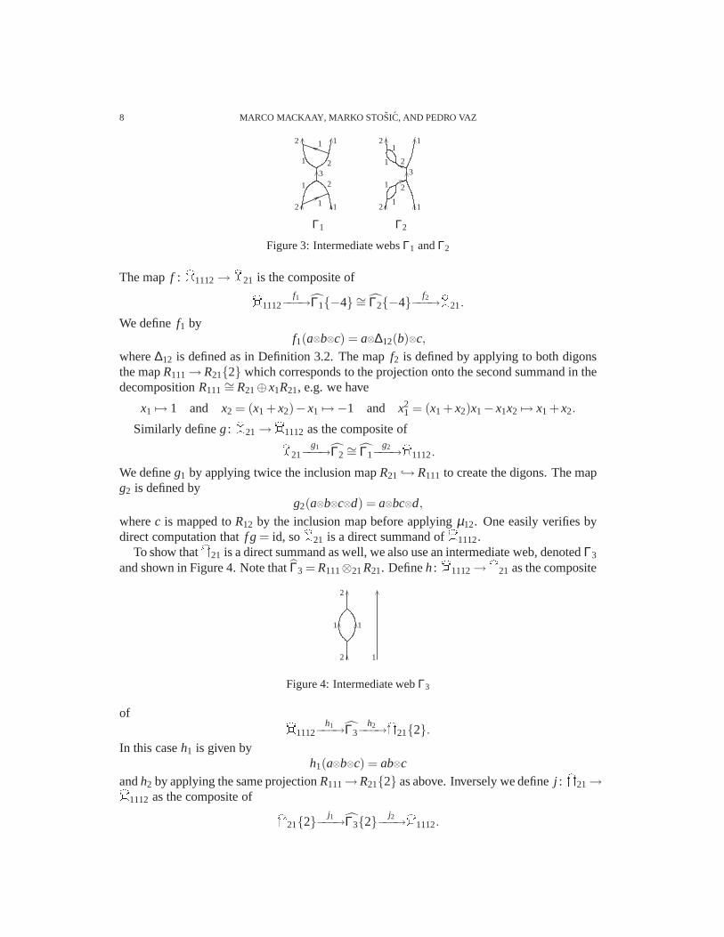
Let Γi be the webs in Figure 3, fori = 1,2. Then we have

Γ1 = R111⊗12R12⊗3 R111⊗21R21∼= R111⊗21R21⊗3 R111⊗21R21

∼= Γ2.


2

2

1

1

1

1

1

1

2

23

2

2

1

1

3

2

2

1

1

1

1

Γ1 Γ2

Figure 3: Intermediate websΓ1 andΓ2

The mapf : t1112→o21 is the composite of

t1112f1−−−→Γ1−4 ∼= Γ2−4

f2−−−→o21.

We definef1 byf1(a⊗b⊗c) = a⊗∆12(b)⊗c,

where∆12 is defined as in Definition 3.2. The mapf2 is defined by applying to both digonsthe mapR111→R212 which corresponds to the projection onto the second summandin thedecompositionR111

∼= R21⊕x1R21, e.g. we have

x1 7→ 1 and x2 = (x1 +x2)−x1 7→ −1 and x21 = (x1 +x2)x1−x1x2 7→ x1 +x2.

Similarly defineg: o21→t1112 as the composite of

o21g1−−−→Γ2

∼= Γ1g2−−−→t1112.

We defineg1 by applying twice the inclusion mapR21 → R111 to create the digons. The mapg2 is defined by

g2(a⊗b⊗c⊗d) = a⊗bc⊗d,

wherec is mapped toR12 by the inclusion map before applyingµ12. One easily verifies bydirect computation thatf g = id, soo21 is a direct summand oft1112.

To show thatr21 is a direct summand as well, we also use an intermediate web, denotedΓ3

and shown in Figure 4. Note thatΓ3 = R111⊗21R21. Defineh: t1112→r21 as the composite

2

2

1

1 1

Figure 4: Intermediate webΓ3

oft1112

h1−−−→Γ3h2−−−→r212.

In this caseh1 is given byh1(a⊗b⊗c) = ab⊗c

andh2 by applying the same projectionR111→R212 as above. Inversely we definej : r21→t1112 as the composite of

r212j1−−−→Γ32

j2−−−→t1112.


The first map is defined by the inclusionR21 → R111. The second map is defined by

j2(a⊗b) = ∆x2,x311 (a)⊗b.

Again, by direct computation, it is straightforward to check thath j =−2id, sor212 is alsoa direct summand oft1112.

Also by direct computation one easily checks thathg = 0 and f j = 0. Finally we haveto show that(g, j) is surjective. Since all maps involved are bimodule maps andR111

∼=R21⊕x2R21 andR111

∼= R12⊕x3R12, we only have to show that 1⊗1⊗1 and 1⊗x2⊗1 are in itsimage. We haveg(1⊗1) = 1⊗1⊗1 and j(1)+ g(x3⊗1) = 1⊗x2⊗1. This finishes the proof ofthe lemma.

Lemma 3.5. Lett1122 be the square in A5. Then we have

t1122∼=o31⊕r312⊕r314.

Proof. The arguments are analogous to the ones used in the proof of Lemma 3.4. To showthato22 is a direct summand oft1122, use the intermediate webs in Figure 5.

3

3

1

1

2

1

2

1

2

24

3

3

1

1

4

3

3

2

2

1

1

Figure 5: Intermediate webs fors1122

With the same notation as before let

f1(a⊗b⊗c) = a⊗∆22(b)⊗c

and for f2 use for both digons the mapR211→ R314 which corresponds to the projectiononto the third direct summand in the decompositionR211

∼= R31⊕x3R31⊕x23R31.

Forg1 we use twice the inclusionR31 → R211 to create the digons and

g2(a⊗b⊗c⊗d) = a⊗bc⊗d.

To show thatr222⊕r224 is a direct summand oft1122 use the intermediate web inFigure 6.

3

3

1

2 1

Figure 6: Intermediate web

Defineh1 byh1(a⊗b⊗c) = ab⊗c


andh2 by applying the mapR211→ R312⊕R314 corresponding to the projection on thelast two direct summands in the decomposition ofR211 above.

For j1 use the mapR312⊕R314 → R211 defined by

(1,0) 7→ 1 and (0,1) 7→ x3

to create the digon. Definej2 by

j2(a⊗b) = ∆x3,x411 (a)⊗b.

An easy calculation shows that

h j =

(1 −x4

0 1

),

which is invertible. This shows thatR312⊕R314 is a direct summand oft1122.Using the rewriting rules for∆22, which were given below its definition, one easily checks

thatg f = 2id. Thereforeo31 is a direct summand oft1122 too.Another easy calculation shows thathg= 0 and a slightly harder one thatf j = 0.Remains to show that(g, j) is surjective. It suffices to show that 1⊗1⊗1,1⊗x3⊗1 and

1⊗x23⊗1 are in its image. We have

1⊗1⊗1 = g(1⊗1)

1⊗x3⊗1 = j(1,0)+g(x4⊗1)

1⊗x23⊗1 = j(0,1)+ j(x4,0)+g(x2

4⊗1)

Lemma 3.6. Lett2113 be the square in A7. We have

t2113∼=o13

22⊕u13222.

Proof. We first define the bimodule map

φ1 : o1322 = R13⊗4 R22→ R121⊗31R211⊗22R22 =t2113.

We use the two intermediate bimodulesΓ1 = R121⊗13R13⊗4 R211⊗22R22 andΓ2 = R121⊗31

R31⊗4 R211⊗22R22 (see Figure 7). Thenφ1 is the composite

2

1

2

3

1

1

1

2

2

3

4

2

1

2

3

4

1

1

3

3

1

2

Γ1 Γ2

Figure 7: Intermediate websΓ1 andΓ2

o

1322

φ11−−−→Γ1

φ21−−−→Γ2

φ31−−−→t2113


with

φ11(a⊗b) = 1⊗a⊗1⊗b

φ21 (a⊗b⊗c⊗d) = ab⊗1⊗c⊗d

φ31 (a⊗b⊗c⊗d) = a⊗bc⊗d.

Conversely we defineψ1 as the composite

t2113ψ1

1−−−→Γ2ψ2

1−−−→Γ1ψ3

1−−−→o1322

with

ψ11(a⊗b⊗c) = a⊗∆31(b)⊗c

ψ21(a⊗b⊗c⊗d) = ab⊗1⊗c⊗d

and withψ31 defined by applying the mapsR121→ R134 andR211→ R222 which are the

projections onto the last direct summands in the decompositionsR121∼= R13⊕x4R13⊕x2

4R13

andR211∼= R22⊕ x3R22. A short calculation shows thatψ1φ1 = −id, which proves thato13

22is a direct summand oft2113.

Let us now defineφ2 : u1322→t2113. Note thatu13

22 = R112⊗22R22. Again we use certainintermediate bimodules:Λ1 = R1111⊗112R112⊗22 R22, Λ2 = R1111⊗211R211⊗22R22, Λ3 =R1111⊗211R211⊗31R211⊗22R22 andΛ4 = R1111⊗121R121⊗31R211⊗22R22 (see Figure 8).

2

1

2

3

1 1

21

2

1

2

3

1

1

1

2

2

1

2

3

123

1

1

1

2

2

1

2

3

1

1

3

2

1

1

2

Λ1 Λ2 Λ3 Λ4

Figure 8: Intermediate websΛ1, . . . ,Λ4

We defineφ2 as the composite

u

1322

φ12−−−→Λ1

φ22−−−→Λ2

φ32−−−→Λ3

φ42−−−→Λ4

φ52−−−→t2113

with

φ11 (a⊗b) = 1⊗a⊗b

φ21 (a⊗b⊗c) = ab⊗1⊗c

φ31 (a⊗b⊗c) = a⊗∆x1x2x3

21 (b)⊗c

φ41 (a⊗b⊗c⊗d) = ab⊗1⊗c⊗d

and withφ51 defined by the mapR1111→ R1212 which is the projection onto the second

direct summand in the decompositionR1111∼= R121⊕x2R121.

Conversely, we defineψ2 as the composite

t2113ψ1

2−−−→Λ4ψ2

2−−−→Λ3ψ3

2−−−→Λ2ψ4

2−−−→Λ1ψ5

2−−−→u1322


with

ψ11(a⊗b⊗c) = 1⊗a⊗b⊗c

ψ21(a⊗b⊗c⊗d) = ab⊗1⊗c⊗d

ψ31(a⊗b⊗c⊗d) = a⊗bc⊗d

ψ41(a⊗b⊗c) = ab⊗1⊗c

and withψ51 defined by the mapR1111→ R1122 which is the projection onto the second

direct summand in the decompositionR1111∼= R112⊕ x3R121. A simple calculation shows

thatψ2φ2 = id.One can also easily check thatψ2φ1 = 0 andψ1φ2 = 0. This shows that(φ1,φ2) is injective.

To show that(φ1,φ2) is surjective note that both maps are leftR13-module maps and that thesource and the target are both freeR13-modules of rank 9 with the same gradings.

4. THE LINK HOMOLOGY

Let us define the coloured HOMFLY-PT homology for links with components labelled 1and 2. We use a similar setup to the one in [3]. To each braid diagram we associate a complexof bimodules (defined below) obtained from the categorified MOY calculus. This complex isinvariant up to homotopy under the braidlike Reidemeister II and III moves. Then we takethe Hochschild homology of each bimodule in the complex, which corresponds to the cate-gorification of the Markov trace. This induces a complex of vector spaces whose homologyis the one we are looking for. The latter is still invariant under the second and third Rei-demeister moves, because the Hochschild homology is a covariant functor, and also underthe Markov moves, as we will show. Therefore we obtain a triply graded link homology. Bytaking the graded dimensions of the homology groups we get a triply graded link polynomial.

To define the complex of bimodules associated to a braid it suffices to define it for a positiveand for a negative crossing only. For an arbitrary braid one then tensors these complexes overall crossings. To each crossing with both strands labelled by 2 we associate a complex withthree terms. For a positive, resp. negative, crossing between strands labelled 2 the terms inthe complex arer226 → t31112 → o22, resp. o22−8 → t3111−8 → r22−6(see Figures 9-10).

= q2q6

2 2 2 2 2

2

2

2

3 1

1

1

2

2

2

2

4d+

1 d+2

Figure 9: The complex of a positive crossing

In both cases, the cohomological degree is fixed by putting the bimoduleo22 in cohomo-logical degree 0.

To define the differentials we need the intermediate websΦ,Ψ and Ω (see Figure 11).Note thatΨ∼= Ω.


= q−6q−8q−8

2 2 2 2

4

2 2

2

2

2

2

3 1

1

1

2 2

d−1 d−2

Figure 10: The complex of a negative crossing

2 2

2

1 1

2

2

2

2

3

3

1

1

1

1

4

2

2

2

2

4

2

2

1

1

1

1

Φ Ψ Ω

Figure 11: Intermediate websΦ, Ψ andΩ

The differentiald+1 is the composite of

r22d+

11−−−→Φd+

12−−−→t3111−4,

whered+11 is defined by the inclusionR22 → R211 to create the digon and

d+12(a⊗b) = ∆x1,x2,x3

21 (a)⊗b.

The differentiald+2 is the composite of

t3111−4d+

21−−−→Ψ−10 ∼= Ω−10d+

22−−−→o22−6,

whered+21 is defined by

d+21(a⊗b⊗c) = a·∆31(b)⊗c

andd+22 by applying twice the mapR211→ R222 given by the projection onto the second

direct summand in the decompositionR211 = R22⊕ x3R22. Direct computation shows thatd+

2 d+1 = 0.

The first differential in the complex associated to a negative crossing is the composite of

o22d−11−−−→Ω∼= Ψ

d−12−−−→t3111,

whered−11 is defined by applying twice the inclusionR22 → R211 to create the digons and

d−12(a⊗b⊗c⊗d) = a⊗bc⊗d.

The differentiald−2 is the composite of

t3111d−21−−−→Φ

d−22−−−→r222,

whered−21 is defined byd−21(a⊗b⊗c) = ab⊗c

andd−22 by applying the same projectionR211→R222 as above. Again, direct computationshows thatd−2 d−1 = 0. Note that this calculation is much easier than the one which showsd+

2 d+1 = 0. The latter is a direct consequence of the former by the observation that all maps


involved in the definition ofd±2 d±1 are units and counits of the two biadjoint functors givenby induction and restriction. As a matter of fact whenever weuse a unit in the definition ofone we use the corresponding counit in the definition of the other. Therefore the fact thatd−2 d−1 = 0 impliesd+

2 d+1 = 0.1

Next we define a complex of bimodules associated to a crossingof a strand labelled 1 anda strand labelled 2. To a positive crossing we associate the complex

= q2

2 1 2 1

1 2

1

2

1

1

2

3d+

and to a negative one

= q−4 q−4

2 1 2 1

1 2

3

2

1

1

2

1d−

Again, in both cases, we put the bimoduleo1221 in the cohomological degree 0.

Note thatu1221 = R111⊗21R21 ando12

21 = R12⊗3 R21. We use the intermediate bimodulesΛ1 = R111⊗21R21⊗3 R21

∼= R111⊗12R12⊗3 R21 = Λ2 (see Figure 12).

2 1

1 2

3

21

1

2

1

1

2

3

1 1

2

Λ1 Λ2

Figure 12: Intermediate websΛ1 andΛ2

Thend+ is the composite of

u

1221

d+1−−−→Λ1−4

∼=−−−→Λ2−4

d+2−−−→o12

21−2

with

d+1 (a⊗b) = a⊗∆21(b)

a⊗b⊗c∼=−→ ab⊗1⊗c

and with d+2 defined by the mapR111→ R122 corresponding to the projection onto the

second direct summand in the decompositionR111∼= R12⊕ x2R12. It is easy to compute the

image ofd+ on generators of theR21−R12 bimoduleR21⊗R111:

d+(1⊗1) = x1⊗1−1⊗x3 and d+(x2⊗1) = 1⊗x1x2−x2x3⊗1.

1We thank Mikhail Khovanov for this observation.


Similarly we defined− as the composite

o

1221

d−1−−−→Λ2∼=−−−→Λ1

d−2−−−→u1221

with

d−1 (a⊗b) = 1⊗a⊗b

a⊗b⊗c∼=−→ab⊗1⊗c

d−2 (a⊗b⊗c) = a⊗bc.

Note that this yieldsd−(a⊗b) = a⊗b.We get similar complexes for the crossings with 1 and 2 swapped. The pictures can be

obtained from the ones above by rotation around they-axis and the shifts are the same.For a crossing with both strands labelled 1 we use the same complex of bimodules as

Khovanov in [3]:

= q2

1 1 1 1 1

1

1

1

2

= q−2 q−2

1 1 1 1

1 1

2

1 1

with v11 in cohomological degree 0.

Let HHH(D) denote the triply graded homology we defined above. Then to obtain the1,2-coloured HOMFLY-PT homologyH1,2(D) we have to apply some overall shifts. Wedefine

Definition 4.1.

H1,2(D) =HHH(D) <n1+−n1

−−s1(D)+2n2+−2n2

−−2s2(D)2 >

−n1

++n1−+s1(D)−2n2

++2n2−+2s2(D)

2 ,−n1

++n1−+s1(D)−2n2

++2n2−+2s2(D)

2

.

The definitions ofni+,ni

− andsi(D) were given in Section 2,< j > is an upward shift byjin the homological degree andk, l denotes an upward shift byk in the Hochschild degreeand byl in theq-degree.

Finally in the following two sections we prove the following

Theorem 4.2. For a given link L, H1,2(D) is independent of the chosen braid diagram Dwhich represents it. Hence, H1,2(L) is a link invariant.


5. INVARIANCE UNDER THE R2 AND R3 MOVES

The next thing to do is to prove invariance of the 1,2-coloured HOMFLY-PT homologyunder the second and third Reidemeister moves. If the strands involved are all labelled 1we already have invariance by Khovanov’s [3] and Khovanov and Rozansky’s [5] results. Ifthere are strands involved which are labelled 2, we will use atrick, inspired by the analogoustrick in [7], which reduces to the case with all link components labelled 1. The argument isslightly tricky, so let us explain the general idea first.

Suppose we have a braidB with n strands, all labelled 2. Create a digonU11 on top ofeach strand. The triply graded polynomial of this braid withdigons is(1+ q2)n times thetriply graded polynomial ofB. We will prove in Lemma 5.2 that sliding the lower parts ofthe digons past the crossings does not change the triply graded polynomial. After slidingthis way the lower parts of all digons past all crossings (seeFigure 13), we obtain a braideddiagramB′ which is the 2-cable ofB with the two top endpoints, and the two bottom end-points respectively, of each cable zipped together. The complex of bimodules associated to

2 2 2 2

2 2

1 11 1

2 2

2 2

1 1 1 1

Figure 13: Creating and sliding digons

B′ is the tensor product of the HOMFLY-PT complex associated tothe 2-cable ofB with twocomplexes, one associated to the top endpoints of the cablesand one to the bottom endpoints.Performing a Reidemeister II or III move onB corresponds to performing a series of Reide-meister II and III moves on its 2-cable. By Khovanov and Rozansky’s [5] results we knowthat the complex of bimodules associated to the 2-cable is invariant up to homotopy equiva-lence under Reidemeister II and III moves. Therefore the complex of bimodules associatedto B′ is invariant under the Reidemeister II and III moves up to homotopy equivalence. Sincethe triply graded polynomial ofB′ is (1+ q2)n times the triply graded polynomial ofB, wesee that the latter is invariant under the Reidemeister II and III moves as well. Note that thismethod does not give a specific homotopy equivalence betweenthe complexes before andafter a Reidemeister move. It only shows that the corresponding Poincare polynomials areequal. This would be a problem if we wanted to show functoriality under link cobordisms ofthe whole construction. However, even the ordinary HOMFLY-PT-homology by Khovanovand Rozansky has not been proven to be functorial and probably is not.

Before we prove the crucial lemma we have to prove an auxiliary result. In the followinglemma the top and the bottom of the diagram are complexes. Thereader can easily check thefollowing auxiliary result.


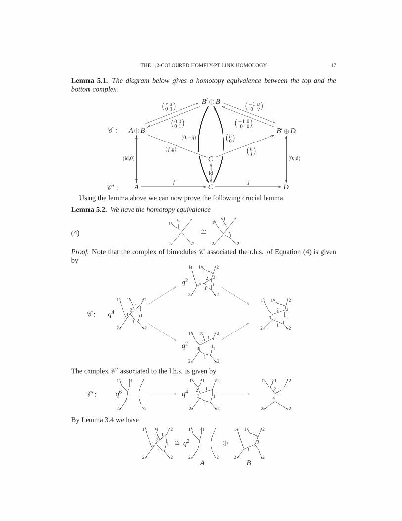
Lemma 5.1. The diagram below gives a homotopy equivalence between the top and thebottom complex.

C :

C ′ :

B′⊕BWW

(h0

)(0,−g)

(0 00 1

)uullllllllllllllllll

(−1 u0 v

)

))SSSSSSSSSSSSSSSSSS

A⊕BOO

(id,0)

( f ,g)))SSSSSSSSSSSSSSSSSSSS

(r s0 1

) 55llllllllllllllllll

B′⊕DOO

(0,id)

(−1 00 0

)iiSSSSSSSSSSSSSSSSSS

C

(hj

)55kkkkkkkkkkkkkkkkkkkk

Af // C

j //

id

OO

D

Using the lemma above we can now prove the following crucial lemma.

Lemma 5.2. We have the homotopy equivalence

(4) ∼=

2

11

2 2

11

2

Proof. Note that the complex of bimodulesC associated the r.h.s. of Equation (4) is givenby

C :

q2

q2

q4

2

1

2

21

12

1

11

2

1

2

21

11

2 3

1

2

1

2

21

3 1

12

1

2

1

2

21

3 1

32

1

The complexC ′ associated to the l.h.s. is given by

C ′ : q6 q4

2

1

2

1

2

1

2

21

3 1

1

1

2

2

1

2

21

4

2

By Lemma 3.4 we have

∼= q2 ⊕

A B2

1

2

21

12

1

1

1

2

1

2

1

2

1

2

21

1

3



∼= ∼= ⊕ q2

B′ B2

1

2

21

12

11

3

2

1

2

21

12

1 1

3

2

1

2

21

1

3

2

1

2

21

1

3


∼= ⊕ q2

B′ D2

1

2

21

1

2

1

1

3

2

1

2

21

34

2

1

2

21

1

3

Note that

∼=4

1 21

2

4

1 21

3

Finally apply Lemma 5.1, which is justified because

(1) d : A→ B is zero,(2) d : B′→ D is zero,(3) d : B→ B is the identity,(4) d : B′→ B′ is minus the identity,

(5) q2 −−→d−−→ q−2 −−→ q−2

2

1 1

2 2

1

2

21

12

1

1

12

1

2

21

31

1

1

12

1

2

21

32 1

11

= q2 d−−→ q−2

2

1 1

2 2

1

2

21

32 1

11

,

and

(6) q−2 −−→ q−2 d−−→ q−4 −−→ q−4

2

1 1

2

2

32 1

1

12

1

2

21

3

21

1

12

1

2

21

3

2 3

11

2

1

2

21

4

2

= q−2 d−−→ q−4

2

1 1

2

2

32 1

1

12

1

2

21

4

2

.

All assertions follow from straightforward computations and can easily be checked. For thefirst assertion one only has to compute the image of 1⊗1, which is zero indeed. For thesecond, third and fourth it suffices to compute the images of 1⊗1⊗1 and 1⊗x1⊗1. For the fifthit suffices to compare the images of 1⊗1. For the sixth one has to compare the images of1⊗1⊗1⊗1, 1⊗1⊗x3⊗1 andx3⊗1⊗1⊗1.


Of course there are also homotopy equivalences analogues tothe one in Lemma 5.2 for anegative crossing or a 11-splitting of the right top strand.

In the following lemma the top and bottom parts are complexesagain.

Lemma 5.3. If s f = 0, the diagram below defines a homotopy equivalence between the topand the bottom complex.

A⊕A′WW

(0f

)(−h,0)

(1,0)vvllllllllllllllllll

(r su −1

)

))SSSSSSSSSSSSSSSSSS

D : AOO

0

h))RRRRRRRRRRRRRRRRRRRRR

(1g

) 66llllllllllllllllll

C⊕A′

(id,−s)

(0 00 −1

)iiSSSSSSSSSSSSSSSSSS

B

( jf

)55kkkkkkkkkkkkkkkkkkkk

D ′ : 0 // Bj //

id

OO

C

(id,0)

OO

Proof. All maps are indicated in the figure, so the reader can check everything easily. Twoidentities are helpful: since the top of the figure is a complex, we have

− jh = r +sg and f h = g−u.

Lemma 5.4. We have the homotopy equivalence

(5) ∼=

1

11

2 1

11

2

Proof. The complex associated to the l.h.s., denotedD ′, is given in Figure 14. The complex

D ′ : q2

1

1

2

11

2

1

1

1

2

11

3

2

Figure 14: Complex of the l.h.s. of Equation (5)

associated to the r.h.s., denotedD , is given in Figure 15.This time we have

∼= ⊕ q2

A A′1

1 1

1 1

2

2 1 2

11

1 2

11


D :

q2

q2

q4

1 2

111 2

21

2

1 1

1

1

2

11

2 1

1

1

2

11

2 1

21

1

Figure 15: Complex of the r.h.s. of Equation (5)

and

∼= ⊕ q2

C A′1 2

1 1 1

2 1

21

11

1

2

11

32

1 2

11

We can apply Lemma 5.3 because

(1) f is equal to the identity,(2) u is equal to minus the identity,(3) s f = 0 and

(4) q−2 d−−→ q−4

1

1 1

2

1

2

11

1

2

11

3

2

= q−2 d−−→ q−4 −−→ q−4 −−→ q−4

1

1 1

2

1

2

11

1

2

11

2

1 2

11

1

1

2

11

32

1

1

2

11

3

2

.

Since we have given all the maps the reader can check the claims by straightforward compu-tations. Note that for the first two claims it suffices to compute the image of 1⊗1. For the lasttwo claims one has to compute the images of 1⊗1⊗1 and 1⊗x2⊗1.

Again, there are analogous homotopy equivalences for a negative crossing or if one swapsthe 1- and 2-strands in the lemma above.

6. INVARIANCE UNDER THE MARKOV MOVES

6.1. Hochschild homology of bimodules as the homology of a Koszulcomplex of poly-nomial rings. The Hochschild homology of a bimodule over the polynomial ring can beobtained as the homology of a corresponding Koszul complex of certain polynomial rings in


many variables. This idea was explained and used by Khovanovin [3]. Here we shall brieflydescribe how to extend it to our case.

First of all, we change our polynomial notation in this section. Namely, the polynomialring Ri1...ik can be represented as the polynomial ring in the variables which are thei1 elemen-tary symmetric polynomials in the firsti1 variables, thei2 elementary symmetric polynomialsin the following i2 variables, etc., and theik elementary symmetric polynomials in the lastikvariables. In this section we will always work with these “new” variables, i.e. the elementarysymmetric polynomials, because it is more convenient for our purposes here. Thus to eachstrand labelled byk, we associate thek variablesx1, . . . ,xk, such that the degree ofxi is equalto 2i, for i = 1, . . . ,k.

To begin with, we describe which polynomial ring to associate to a web. Take a weband choose a height function to separate the vertices according to height. This way chop upthe web into several layers with only one vertex. To each layer we associate a new set ofvariables. To each vertex with incident edges labelledi, j and i + j we associate thei + jpolynomials which are the differences of thek-th symmetric polynomials in the outgoingvariables and the incoming variables, for everyk = 1, . . . , i + j. Moreover, if there are twodifferent sets of variablesx1, . . . ,xk andx′1, . . . ,x

′k associated to a given edge labelledk, we

also associate thek polynomialsxi − x′i, for all i = 1, . . . ,k. Finally, to the whole graph weassociate the polynomial ring in all the variables modded out by the ideal generated by all thepolynomials associated to the vertices and edges.

There is an isomorphism between these polynomial rings and the corresponding bimodulesassociated to the graph. Indeed, to the tensor productp(x)⊗q(x) in variablesx, correspondsthe polynomialp(x′)q(x), where the variablesx are of the bottom layer, andx′ are of the toplayer. Loosely speaking, the position of the factor in the tensor product corresponds to thesame polynomial in the variables corresponding to the layer.

Let us do an example:

Example 6.1. Consider the webl21:

2 1

3

2 1

x1,x2 y1

x′1,x′2 y′1

The polynomial ring associated to this web is the ring Pl21

:= C[x1,x2,y1,x′1,x′2,y′1]. The

ideal Il21

by which we have to quotient, is generated by the differencesof the symmetricpolynomials in all top and bottom variables (since the middle edge is labelled by 3). Thereare three elementary symmetric polynomial in this case:Σ1 = x1 + y1, Σ2 = x2 + x1y1 andΣ3 = x2y1, and so

Il21

= 〈x1 +y1−x′1−y′1,x2 +x1y1−x′2−x′1y′1,x2y1−x′2y′1〉.

Hence, the polynomial ring we associate to it is given by

Rl21

= Pl21

/Il21

.

On the other hand, the bimoduleo21 associated to the webl21 is R21⊗3 R21, and itselements are linear combination of elements of the form p(x1,x2,y1)⊗q(x1,x2,y1), for some


polynomials p and q. Finally, the isomorphism betweeno21 and Rl21

is given by:

p(x1,x2,y1)⊗q(x1,x2,y1)←→ p(x′1,x′2,y′1)q(x1,x2,y1).

In such a way we have obtained the bijective correspondence between the bimodulesΓ andthe polynomial ringsRΓ that are associated to the open trivalent graphΓ. The closure ofΓ inthe bimodule picture corresponds to taking the Hochschild homology ofΓ. In the polynomialring picture this is isomorphic to the homology of the Koszulcomplex overRΓ which is thetensor product of the the complexes

(6) 0−−→ RΓ−1,2i−1xi−x′i−−−−→RΓ −−→ 0,

where thexi ’s are the bottom layer variables, and thex′i ’s are the top layer variables. We putthe right-hand side term in (co)homological degree zero. The first shift is in the Hochschild(homological) degree, and the second one is in theq-degree, so that the maps have bi-degree(1,1).

6.2. Invariance under the first Markov move. Essentially we have to show that the Hochs-child homology of the tensor productB1⊗B2 of the bimodulesB1 andB2 is isomorphic tothe Hochschild homology ofB2⊗B1, i.e.

(7) HH(B1⊗B2) = HH(B2⊗B1).

We shall prove this by passing to the polynomial ring and Koszul complex descriptionfrom above. Recall, that to the open trivalent graphΓ we have associated the polynomialalgebraPΓ (the ring of polynomials in all variables) quotiented by theideal IΓ generated bycertain polynomials. Since for each layer we introduced newvariables, the sequence of thesepolynomials is regular and so we have thatRΓ = PΓ/IΓ is the homology of the Koszul complexobtained by tensoring together all complexes of the form

0−−→ PΓf−→PΓ −−→ 0,

for f ∈ IΓ. We call this the Koszul complex generated byIΓ.Finally, the object associated to the closure of the graphΓ is given by the homology of

the Koszul complex defined by (6), and so it is isomorphic to the homology of the Koszulcomplex generated by the polynomials which defineIΓ together with the polynomialsxi −x′iwhich come from the closure. IfΓ is the vertical glueing ofΓ1 andΓ2 then inIΓ we have thepolynomialsy j−y′j which correspond to the edges which are glued together. The Hochschild

homology ofΓ1⊗ Γ2 is isomorphic to the homology generated byIΓ1, IΓ2 and the polynomialsxi −x′i andy j −y′j . Clearly the same holds forΓ2⊗ Γ1, with the role of thexi −x′i andy j −y′jinterchanged. Thus we have proved (7).

6.3. Invariance under the second Markov move. Invariance under the second Markovmove corresponds to invariance under the Reidemeister moveI. If the strand involved islabelled 1, the result was proved by Khovanov and Khovanov and Rozansky [3, 5] (see be-low).


Remains to show invariance if the strand is labelled 2. For both the positive and the nega-tive crossing, we have the same three resolutions:

2 2 2 2

3 1

2 2

1

1

2 2

2 2

4

For each of these, we shall give its description in a polynomial language, and compute thehomology of the corresponding Koszul complex.

The resolutionq: Before closing the right strand, we have an open graph. To the bottomlayer we associate variablesx1 andx2 to the left strand, andy1 andy2 to the right strand, whileto the top layer we associate variablesx′1 andx′2 to the left strand, andy′1 andy′2 to the rightstrand. Then the ringR

q

we associate to it, is the ring of polynomials in all these variablesmodded out by the ideal generated by the polynomialsx′1− x1, x′2− x2, y′1− y1 andy′2− y2,i.e. it is isomorphic to the ring

B := C[x1,x2,y1,y2].

The resolutions: The variables that we associate to the bottom and the top layers are thesame as above. To the bottom middle strand we associate variablez1, to the top middle strandwe associatez′1 and to the right strand we associate variablet1. Then the corresponding ringRs

is the ring of polynomials in all these variables, modded outby the ideal generated by thepolynomialsy1−z1−t1, y2−z1t1, y′1−z′1−t1, y′2−z′1t1, x1+z1−x′1−z′1, x2+x1z1−x′2−x′1z′1,x2z1−x′2z′1. From the first four relations, we can excludet1 and obtain the quadratic relationsfor z1 and z′1: z2

1 = y1z1− y2 and z′12 = y′1z′1− y′2. Hence, every element fromR

s

can bewritten asa+bz1 +cz′1+dz1z′1, wherea, b, c andd are polynomials only inx’s andy’s (withor without primes).

The resolutionl: The variables we associate to the bottom and top layers are again thesame. This time, the ringR

l

we obtain by quotienting by the ideal generated by the followingfour polynomials:x1 +y1−x′1−y′1, x2 +y2+x1y1−x′2−y′2−x′1y′1, x2y1 +x1y2−x′2y′1−x′1y′2andx2y2−x′2y′2.

To the closure of the right strands of each of these graphs, corresponds the homology ofthe tensor product of the following two Koszul complexes:

0 −−→ RΓ−1,1y1−y′1−−−→ RΓ −−→ 0,

0 −−→ RΓ−1,3y2−y′2−−−→ RΓ −−→ 0.

Hence, in all three cases we can have homology in three homological gradings 0,−1 and−2. We denote this homology byHHR(Γ).


In the case ofq we have that both differentials are 0. Hence

HHR0 (q) = B = C[x1,x2,y1,y2],

HHR−1(q) = B1⊕B3,

HHR−2(q) = B4.

For the other two cases the computations are a bit more involved and we want to explainthe general idea first. The Hochschild homology is the homology of a complex which is thetensor product of complexes of the form

0 −−→ P/Ip−→ P/I −−→ 0,

whereP is a polynomial ring,I is an ideal andp∈ R is a polynomial. Let us explain how tocompute the homology of one such complex.

The main part is the computation of the kernel and the cokernel of the map above. Thecokernel is easily computed, and is equal to the quotient ring P/〈I , p〉. Now, let us pass to thekernel. For any polynomialq∈P to be in the kernel, i.e. to be a cocycle, we must havepq∈ I .The ideals are always finitely generated, sayI is generated byi1, . . . , in. Therefore we have tofind all solutions to the equationa1i1+ · · ·+anin = pq, i.e. we rewritea1i1+ · · ·+anin until itbecomes of the formp times something, which imposes constraints on theai . The solutionsare generated byq1, . . . ,qk, which generate an idealQ (in the cases we are interested in, it isalways a principal ideal, i.e.Q = qP, for someq∈ P). Then the kernel is given byQ/I (i.e.qP/I ). However, this is isomorphic toQ/〈I , p〉, sincepqs ∈ I for all s, which is the form inwhich we present the results below.

It is not hard to extend these calculations to a tensor product of complexes of the aboveform. In particular, all homologies are certain ideals, modded out by the ideal generated byIΓ and the polynomialsyi − y′i , i = 1,2, which in particular includes the polynomialsxi − x′i,i = 1,2 and alsoz1−z′1 in the case of the webs. Hence, in the homology, all variables withprimes are equal to the corresponding variables without theprimes.

In the case ofs, we have thaty2−y′2 = t1(z1−z′1) = (y1−z1)(y1−y′1), and straightforwardcomputations along the lines sketched above give

HHR0 (s) = A = C[x1,x2,y1,y2,z1]/〈z

21−y1z1 +y2〉,

HHR−1(s) = ((y1−z1)g+(x2−y2−z1(x1−y1))h) ,g)|g,h∈ A ⊂ A1⊕A3,

HHR−2(s) = (x2−y2−z1(x1−y1))A4.

Note that we haveA∼= B⊕z1B.Finally, in the case ofl, we obtain

HHR0 (l) = B = C[x1,x2,y1,y2],(8)

HHR−1(l) = (−c(x2−y2)+ (cy1 +dy2)(x1−y1),c(x1−y1)+d(x2−y2)) |c,d ∈ B(9)

⊂ B1⊕B3,

HHR−2(l) = pB4,(10)

wherep = (x2−y2)2 +(x1−y1)(x1y2−x2y1).


Now, we pass to the differentials. In our polynomial notation, in the case of the positivecrossing, the maps are (up to a non-zero scalar):

Rq

→ Rs

−4 : 1 7→ (x2 +x′2−y2−y′2)+ (y1−x′1)z1 +(y′1−x1)z′1.

In the case of the second map (s→ q−2l), it is given by the coefficient ofz1z′1 after

multiplication with

(−y31 +2y1y2 +x′1(y

21−y2)−x′2y1−y′31 +2y′1y′2 +x1(y′1

2−y′2)−x2y′1)+ (z1 +z′1)(x2−x1y′1 +y′1

2−y′2+x′2−x′1y1 +y21−y2)+

+ z1z′1(x1 +x′1−y1−y′1).

Recall that the elements ofRs

are of the forma+bz1 +cz′1 +dz1z′1, wherea, b, c andd arethe polynomials only inx’s andy’s, while z2

1 = y1z1−y2 andz′12 = y′1z′1−y′2.

For the negative crossing, the maps are the following

Rl

→ Rs

: 1 7→ 1,

and

Rs

→ Rq

2 : a+bz1 +cz′1 +dz1z′1 7→ b+c+dy1.

Since we are interested in the differentials in the case whenthe right strands are closed,in the homology all variables with primes are equal to the ones without the primes (as weexplained above), and the differentials reduce to the following (again up to a non-zero scalar)

→ q−4 : 1 7→ (x2−y2)− (x1−y1)z1,

→ q−2 : a+bz1 7→ a(x1−y1)+b(x2−y2),

→ : 1 7→ 1,

→ q2 : a+bz1 7→ b,

wherea,b∈ B.

Now, by straightforward computation of the homology for both positive and negativecrossing in each Hochschild degree, we obtain the followingsimple behaviour of HHH under


the Reidemeister I move:

HHH

(

2

)= HHH

(

2

),

HHH

(

2

)= HHH

(

2

)< 2 > −2,−2.

We recall that< i > denotes the upward shift byi in the homological degree, whilek, ldenotes the upward shift byk in the Hochschild degree and byl in theq-degree.

For the Reidemeister I move involving a strand labelled 1, weget a similar shift (see [3, 5],or apply the same methods as above):

HHH

(

1

)= HHH

(

1

),

HHH

(

1

)= HHH

(

1

)< 1 > −1,−1.

The overall shift in the definition ofH2(D) compensates this behaviour under the Reidemeis-ter I moves and we get a genuine link invariant.

6.4. Categorification of the axioms A1 and A2. In this subsection we shall show that ourconstruction categorifies the axioms A1 and A2 of the MOY calculus, that include the clo-sures of the strands. The powers ofq in A1 and A2 will correspond to the internalq-grading(grading of the polynomial ring), while the powers oft will correspond to the Hochschildgrading.

First we focus on the A1 axiom for arbitraryk. The circle is the closure of the single strandlabelled withk. Denote the graph that consists of this strand bywk, and the variables that weassociate to it byx1, . . . ,xk (remember that in this section we assume that degxi = 2i). Then tothiswk we associate the ringR

wk= C[x1, . . . ,xk], and to its closure, the Hochschild homology

HH(wk), which is the homology of the Koszul complex obtained by tensoring

0−−→ Rwk−1,2i−1

0−→R

wk−−→ 0,

for all i = 1, . . . ,k. Hence we have

HH(wk) =k⊗

i=1

(C[x1, . . . ,xk]⊕C[x1, . . . ,xk]−1,2i−1),

which categorifies the axiom A1.

Now we consider the axiom A2. The left hand side of the axiom isthe closure of the rightstrand of the graph that we denoted byli j . As we said previously, we are only interestedin the cases when the indicesi and j are from the set1,2, and so we have four cases.Each of these cases we treat in the same way as the case ofl22 which we dealt with in theprevious subsection. We associate the variablesx1, . . . ,xi andx′1, . . . ,x

′i to the strands on the


left-hand side and the variablesy1, . . . ,y j andy′1, . . . ,y′j to the strands on the right-hand side,

and compute the homology (that we denote byHHR(li j )) of the tensor product of the Koszulcomplexes

0−−→ Rli j−1,2l −1

yl−y′l−−−−→Rli j−−→ 0,

for l = 1, . . . , j. In the remaining part of the graph, the variablesy don’t appear again, whileas before, in theHHR(li j ) we have thatxl = x′l , for all l = 1, . . . , i. Finally, the right handside of the axiom A2 iswi to which we associate the variablesx1, . . . ,xi , and consequentlythe ringR

wi= C[x1, . . . ,xi ].

Now, in the four cases we are interested in, the homologies are the following:

i = j = 1 : The corresponding ring in this case isRl11

= C[x1,x′1,y1,y′1]/〈x1 + y1− x′1−y′1,x1y1−x′1y′1〉, while HHR

l11is the homology of the complex

0−−→ Rl11−1,1

y1−y′1−−−−→Rl11−−→ 0.

Direct computation of this homology gives

HHR0 (l11) = C[x1,y1],

HHR−1(l11) = (x1−y1)C[x1,y1]1,

which categorifies A2 in this case.

i = 2, j = 1 : The corresponding ring in this case isRl21

= C[x1,x2,x′1,x′2,y1,y′1]/〈x1+y1−

x′1−y′1,x1y1 +x2−x′1y′1−x′2,x2y1−x′2y′1〉, while HHRl21

is the homology of the complex

0−−→ Rl21−1,1

y1−y′1−−−−→Rl21−−→ 0.

Then we have

HHR0 (l21) = C[x1,x2,y1],

HHR−1(l21) = (x2−x1y1 +y2

1)C[x1,x2,y1]1,

as wanted.

i = 1, j = 2 : The corresponding ring in this case isRl12

= C[x1,x′1,y1,y2,y′1,y′2]/〈x1 +

y1−x′1−y′1,x1y1 +y2−x′1y′1−y′2,x1y2−x′1y′2〉, while HHRl12

is the homology of the complexobtained by tensoring

0−−→ Rl12−1,1

y1−y′1−−−−→Rl12−−→ 0,

and

0−−→ Rl12−1,3

y2−y′2−−−−→Rl12−−→ 0.


Thus, we obtain

HHR0 (l12) = C[x1,y1,y2],

HHR−1(l12) = (c(x1−y1)+dy2,−c+dx1)) |c,d ∈ C[x1,y1,y2]

⊂ C[x1,y1,y2]1⊕C[x1,y1,y2]3,

HHR−2(l12) = (x2

1−x1y1 +y2)C[x1,y1,y2]4,

which categorifies A2 in this case.

i = j = 2 : This case we have already computed in the previous subsection, in the formulas(8)-(10), which gives the categorification of A2 in this case.

7. CONJECTURES ABOUT THE HIGHER FUNDAMENTAL REPRESENTATIONS

Ideas similar to the ones in this paper will probably work forlink components labelledwith arbitrary MOY labels.

First of all, to the open MOY webΓ we associate the bimoduleΓ in the same way. In orderto define the resolutions for the crossings, in principal oneonly has to know which maps toassociate to the zip, the unzip, the digon creation and the digon annihilation. For the zip andthe unzip our candidates are given in the following definition.

Definition 7.1. We define the linear maps

µi j : oi j →ri j and ∆i j : ri j →oi j

by

µi j (a⊗b) = ab

and

∆i j (1) = ∑α=(α1,...,αi )j≥α1≥···αi≥0

(−1)|α |πα ⊗π ′α∗,

whereα∗ is the conjugate partition of the complementary partitionα∗ = ( j−ai , . . . , j−a1),andπα (respectivelyπ ′β ) is the Schur polynomial in the firsti variables (respectively, lastjvariables). The conjugate (dual) partition of the partition β = (β1, . . . ,βk), is the partitionβ = (β1, β2, . . .), whereβ j = ♯i|βi ≥ j.

The proof of the following lemma will be part of a forthcomingpaper:

Lemma 7.2. µi j and∆i j are Ri j -bimodule maps.

Note that the lemma above implies that∆i j is the coproduct in the commutative FrobeniusextensionH∗U(i+ j)

(G(i, i + j)) with respect to the trace defined by tr(π j... j) = 1.The digon creation and annihilation maps are deduced from Lemma 3.1.Before we explain the complexes that we associate to the crossings, we call attention to

the following isomorphisms.


∼=

a b

a+c+d b−c−d

a+cb−c

c

d

a b

a+c+d b−c−d

b−c

c+d

c

d

∼=

a b

a−c−d b+c+d

a−cb+c

c

d

a b

a−c−d b+c+d

c+d

b+c

c

d

To each positive crossing such thati ≤ j we associate a complex of resolutions (see Fig-ure 16)

Γ0i(i +1)d+

0−−−→Γ1(i−1)id+

1−−−→Γ2(i−2)(i−1)d+

2−−−→·· ·d+

i−1−−−−→Γi,

where we putΓi in the homological degree 0. Our candidates for the differentials are indicatedin Figure 17. Note that we have used the isomorphisms above.

j i j

i

i

j

j +k i−k

k

j +k− i

j i

Γk

Figure 16: A positive crossing, the webΓk, and a negative crossing

To negative crossings withi ≤ j, we associate the following complex of bimodules:

Γi−2i jd+

0−−−→Γi−1−2i jd+

1−−−→Γi−22−2i jd+

2−−−→·· ·d+

i−1−−−−→Γ0(i−1)i−2i j,

where again we put the resolutionΓi in the homological degree 0. The differentials are ob-tained by inverting all arrows in the Figure 17.

In the case wheni < j, by looking at the picture from the “other side of the paper” (i.e. byrotation around they-axis), we obtain the crossing of the above form.

The following lemma is hard to prove directly, as one has to check the statement for a lotof generators. However in a subsequent paper we will prove this conjecture using a differenttechnique.

Conjecture 1. d±k+1d±k = 0, for all 0≤ k≤ i−2.

The other tricks remain largely the same. The crucial conjecture to prove is

Conjecture 2. We have the homotopy equivalence

∼=

j

1i

i +1 j

1i

i +1


q−2( j+k)

q−2( j+k) q−2( j+k) q2(k−i)

j

i

i

j

j +k

i−k

k

j +k− i

j

i

i

j

j +k

i−k

i−k

k

j +k− i

1i− (k+1)

j

i

i

j

j +k+1

j +k

j +k

i−k

i−k

k

j +k− i

i− (k+1)

1

1

j

i

i

j

j +k+1

j +k− i +1

i− (k+1)

i−k

i−k

k+1

j +k− i

k

1

1

j

i

i

j

j +k+1

i− (k+1)

k+1

k

j +k− i +1

j +k− i

1

1

j

i

i

j

j +k+1

i− (k+1)

k+1

j +k− i +1

Figure 17: The definition of the differentials

AcknowledgementsThe authors thank Mikhail Khovanov and Catharina Stroppel for helpfulconversations on the topic of this paper.

The authors were supported by the Fundacao para a Cienciae a Tecnologia (ISR/IST pluri-anual funding) through the programme “Programa Operacional Ciencia, Tecnologia, Inova-cao” (POCTI) and the POS Conhecimento programme, cofinanced by the European Com-munity fund FEDER. Marko Stosic is also partially supportedby the Ministry of Science ofSerbia, project 144032.

REFERENCES

[1] W. Fulton,Equivariant cohomology in algebraic geometry, Eilenberg lectures, Columbia University, spring2007, available at http://www.math.lsa.umich.edu/∼dandersn/eilenberg/.

[2] S. Gukov, A. Iqbal, C. Kozcaz, C. Vafa, Link Homologies and the Refined Topological Vertex, preprint2007, arXiv:0705.1368.

[3] M. Khovanov, Triply-graded link homology and Hochschild homology of Soergel bimodules,Int. J. Math.18(8):869-885, 2007.

[4] M. Khovanov and L. Rozansky, Matrix factorizations and link homology,Fund. Math.199(1):1-91, 2008.[5] M. Khovanov and L. Rozansky, Matrix factorizations and link homology II,Geom. Topol.12:1387-1425,

2008.[6] M-J. Jeong and D. Kim, Quantumsl(n,C) link invariants, preprint 2005, arXiv:math/0506403v2 [math.GT].[7] H. Murakami, T. Ohtsuki, S. Yamada, HOMFLY-PT polynomial via an invariant of colored plane graphs,

Enseign. Math.(2) 44: 325-360, 1998.[8] J. Rasmussen, Some differentials on Khovanov-Rozanskyhomology, preprint 2006, arXiv:math/0607544v2

[math.GT].

http://www.math.lsa.umich.edu/~dandersn/eilenberg/

http://arxiv.org/abs/0705.1368

http://arxiv.org/abs/math/0506403

http://arxiv.org/abs/math/0607544


[9] B. Webster, G. Williamson, A geometric model for Hochschild homology of Soergel bimodules,Geom.Topol.12:1243-1263, 2008.

[10] H. Wu, Matrix factorizations and colored MOY graphs, preprint 2008, arXiv:0803.2071v3 [math.GT].[11] Y. Yonezawa, Matrix factorizations and intertwiners of the fundamental representations of quantum group

Uq(sln), preprint 2008, arXiv:0806.4939v1 [math.QA].

DEPARTAMENTO DEMATEMATICA , UNIVERSIDADE DO ALGARVE, CAMPUS DE GAMBELAS , 8005-139FARO, PORTUGAL AND CAMGSD, INSTITUTO SUPERIORTECNICO, AVENIDA ROVISCO PAIS, 1049-001L ISBOA, PORTUGAL

E-mail address: [email protected]

INSTITUTO DE SISTEMAS E ROBOTICA AND CAMGSD, INSTITUTO SUPERIORTECNICO, AVENIDA RO-VISCO PAIS, 1049-001 LISBOA, PORTUGAL


DEPARTAMENTO DEMATEMATICA , UNIVERSIDADE DO ALGARVE, CAMPUS DE GAMBELAS , 8005-139FARO, PORTUGAL AND CAMGSD, INSTITUTO SUPERIORTECNICO, AVENIDA ROVISCO PAIS, 1049-001L ISBOA, PORTUGAL




The 1,2-coloured HOMFLY-PT link homology

Documents

Transcript of The 1,2-coloured HOMFLY-PT link homology