Seventh Workshop and Tutorial on Practical Use of Coloured ...

DEPARTMENT OF COMPUTER SCIENCE UNIVERSITY OF AARHUS

IT-parken, Aabogade 34 DK-8200 Aarhus N, Denmark

ISSN 0105-8517

October 2006

DAIMI PB - 579

Kurt Jensen (Ed.)

Seventh Workshop and Tutorial on Practical Use of Coloured Petri Nets and the CPN Tools Aarhus, Denmark, October 24-26, 2006

Preface This booklet contains the proceedings of the Seventh Workshop on Practical Use of Coloured Petri Nets and the CPN Tools, October 24-26, 2006. The workshop is organised by the CPN group at Department of Computer Science, University of Aarhus, Denmark. The papers are also available in electronic form via the web pages: http://www.daimi.au.dk/CPnets/workshop06/

Coloured Petri Nets and the CPN Tools are now used by more than 4000 users in 124 countries. The aim of the workshop is to bring together some of the users and in this way provide a forum for those who are interested in the practical use of Coloured Petri Nets and their tools.

The submitted papers were evaluated by a programme committee with the following members:

Wil van der Aalst, Netherlands João Paulo Barros, Protugal Jonathan Billington, Australia Jörg Desel, Germany Joao M. Fernandes, Portugal Jorge de Figueiredo, Brazil Monika Heiner, Germany Kurt Jensen, Denmark (chair) Ekkart Kindler, Germany Lars M. Kristensen, Denmark Johan Lilius, Finland Tadao Murata, USA Daniel Moldt, Germany Laure Petrucci, France Robert Valette, France Rüdiger Valk, Germany Lee Wagenhals, USA Jianli Xu, Finland Karsten Wolf, Germany

The programme committee has accepted 15 papers for presentation. Most of these deal with different projects in which Coloured Petri Nets and their tools have been put to practical use – often in an industrial setting. The remaining papers deal with different extensions of tools and methodology.

The papers from the first six CPN Workshops can be found via the web pages: http://www.daimi.au.dk/CPnets/. After an additional round of reviewing and revision, some of the papers have also been published as special sections in the International Journal on Software Tools for Technology Transfer (STTT). For more information see: http://sttt.cs.uni-dortmund.de/ Kurt Jensen

Table of Contents Lars M. Kristensen, Peter Mechlenborg, Lin Zhang, Brice Mitchell, and Guy E. Gallasch Model-based Development of a Course of Action Scheduling Tool ......................... 1 Jens Bæk Jørgensen, Kristian Bisgaard Lassen, and Wil M. P. van der Aalst From Task Descriptions via Coloured Petri Nets Towards an Implementation of a New Electronic Patient Record......................................................................... 17 Cong Yuan and Jonathan Billington A Coloured Petri Net Model of the Dynamic MANET On-demand Routing Protocol .................................................................................................................... 37 A. Rozinat, R.S. Mans, and W.M.P. van der Aalst Mining CPN Models Discovering Process Models with Data from Event Logs ....................................... 57 M.H. Jansen-Vullers and M. Netjes Business Process Simulation - A Tool Survey ........................................................ 77 Michael Westergaard The BRITNeY Suite: A Platform for Experiments.................................................. 97 Guy Edward Gallasch, Nimrod Lilith, Jonathan Billington, Lin Zhang, Axel Bender, and Benjamin Francis Modelling Defence Logistics Networks ................................................................ 117 F. Gottschalk, W.M.P. van der Aalst, M.H. Jansen-Vullers, and H.M.W. Verbeek Protos2CPN: Using Colored Petri Nets for Configuring and Testing Business Processes................................................................................................................ 137 Somsak Vanit-Anunchai, Jonathan Billington and Guy Edward Gallasch Sweep-line Analysis of DCCP Connection Management ..................................... 157 Hendrik Oberheid A Colored Petri Net Model of Cooperative Arrival Planning in Air Traffic Control ................................................................................................. 177 Vijay Gehlot and Anush Hayrapetyan A CPN Model of a SIP-Based Dynamic Discovery Protocol for Webservices in a Mobile Environment ....................................................................................... 197 P.M. Kwantes Design of Clearing and settlement operations: A case study in business process modelling and evaluation with Petri nets.......... 217 Óscar R. Ribeiro and João M. Fernandes Some Rules to Transform Sequence Diagrams into Coloured Petri Nets ............. 237 Invited Talk: Karsten Wolf Inside LoLA - Experiences from Building a State Space Tool for Place Transition Nets ............................................................................................. 257 Suratose Tritilanunt, Colin Boyd, Ernest Foo, and Juan Manuel González Nieto Using Coloured Petri Nets to Simulate DoS-resistant protocols ........................... 261 M. Westergaard Game Coloured Petri Nets ..................................................................................... 281

Model-based Development of a

Course of Action Scheduling Tool

Lars M. Kristensen1, Peter Mechlenborg1,Lin Zhang2, Brice Mitchell2, and Guy E. Gallasch3

1 Department of Computer Science, University of AarhusIT-parken, Aabogade 34, DK-8200 Aarhus N, DENMARK,

{lmkristensen,metch}@daimi.au.dk2 Defence Science and Technology Organisation

PO Box 1500, Edinburgh, SA 5111, AUSTRALIA{Lin.Zhang, Brice.Mitchell}@dsto.defence.gov.au

3 Computer Systems Engineering Centre, University of South Australia,Mawson Lakes Campus, SA 5095, AUSTRALIA

[email protected]

Abstract. This paper shows how a formal method in the form of Colou-red Petri Nets (CPNs) and the supporting CPN Tools have been usedin the development of the Course of Action Scheduling Tool (COAST).The aim of COAST is to support human planners in the specificationand scheduling of tasks in a Course of Action. CPNs have been usedto develop a formal model of the task execution framework underlyingCOAST. The CPN model has been extracted in executable form fromCPN Tools and embedded directly into COAST, thereby automaticallybridging the gap between the formal specification and its implementa-tion. The scheduling capabilities of COAST are based on state space ex-ploration of the embedded CPN model. Planners interact with COASTusing a domain-specific graphical user interface (GUI) that hides the em-bedded CPN model and analysis algorithms. This means that COASTis based on a rigorous semantical model, but the use of formal methodsis transparent to the users. Trials of operational planning using COASThave been conducted within the Australian Defence Force.

Keywords: Application of Coloured Petri nets, State space analysis,Scheduling, Command and Control, Methodologies, Tools.

1 Introduction

Planning and scheduling [6] are activities performed in many domains such asbuilding construction, natural disaster relief operations, search and rescue mis-sions, and military operations. Planning is a major challenge due to severalfactors, including time pressure, ambiguity in guidance, uncertainty, and com-plexity of the problem. The development of computer tools that can aid plannersin developing and analysing Courses of Actions such that they meet their objec-tives is therefore of key interest in many application domains. Recently, there has

been an increased interest in the application of formal methods and associatedanalysis techniques in the planning and scheduling domain (see, e.g., [1, 3, 11]).

This paper presents the Course of Action Scheduling Tool (COAST) beingdeveloped for the Australian Defence Force (ADF) by the Australian DefenceScience and Technology Organisation (DSTO). The aim of COAST is to sup-port planners in Course of Action (COA) development and analysis which aretwo of the main activities in planning processes within the ADF. The frame-work underlying COAST has been deliberately made generic in order to makeCOAST applicable to a broad spectrum of domains, and so not restricting itsapplicability to the military planning domain. The basic entities in a COA (rep-resenting a planning problem) are tasks which have associated pre- and post-conditions describing the conditions required for a task to execute and the effectof executing the task. The dependencies between tasks expressed via conditionscapture the logical structure of a COA. The execution of a task also requiresresources ; a subset of which are released in accordance with the specificationswhen the task terminates. Task synchronisations make it possible to directlyspecify temporal and precedence information for tasks, e.g., a set of tasks muststart simultaneously. The main analysis capability of COAST is the computationof task schedules called lines of operation (LOPs) which are execution sequencesof tasks that lead from an initial state to a desired goal state which is a state inwhich a certain set of conditions are satisfied. COAST also supports the plannersin debugging and identifying errors in COAs.

The development of COAST has been driven by the use of formal methodsin the form of Coloured Petri Nets (CP-nets or CPNs) [7,8] and the supportingcomputer tool CPN Tools [2]. CPN modelling was chosen because CP-nets sup-port construction of compact parametriseable models, support structured datatypes, make it possible to model time, and allow models to be hierarchicallystructured into a set of modules.

The basic idea behind the development of COAST has been to use CP-netsto develop, formalise, and implement the task execution framework which formsthe core of COAST. The CPN model formalises the execution of tasks accordingto the pre- and postconditions of tasks, imposed synchronisations, and assignedresources. The concrete tasks, conditions, synchronisations, and resources thatmake up the COA to be analysed are represented as tokens populating theCPN model. The analysis capabilities of COAST are based on state space ex-ploration [14]. State space exploration relies on computing all reachable statesand state changes of the system and representing these as a directed graphwhere nodes represent reachable states and arcs represent occurring events. Twoalgorithms are implemented for computing lines of operation: a two-phase algo-rithm consisting of a depth-first state space generation followed by a breadth-firsttraversal, and an algorithm that is based on the so-called sweep-line method [10].The CPN model and the analysis algorithms that form the core of COAST havebeen hidden behind a domain-specific graphical user interface. This makes theuse of the underlying formal method transparent to the planners who cannot beexpected to be familiar with CP-nets and state space methods.

A preliminary version of the task execution framework of COAST has beeninformally presented in [15,16] together with the graphical user interface. Someearly algorithms for computing lines of operation were presented in [9]. The con-tribution of this paper is to present the formal engineering aspects of COASTin the form of the underlying CPN model and the new state space explorationalgorithms implemented for obtaining lines of operation. We also demonstratehow the sweep-line method [10] can be applied to the planning domain. Fur-thermore, we explain how COAST has been engineered via embedding of anexecutable CPN model. The latter demonstrates how formal methods in theform of CP-nets can be used in software development.

The rest of the paper is organised as follows. Section 2 presents the method-ology used for the formal engineering of COAST. Section 3 presents selectedparts of the CPN model that formalises the task execution framework. Section 4presents the state space exploration algorithms for generating lines of operation.Finally, we sum up the conclusions in Sect. 5. The reader is assumed to be fa-miliar with the CPN modelling language and the basic ideas behind state spacemethods.

2 Formal Engineering Methodology

COAST is based on a client-server architecture. The client constitutes the domain-specific graphical user interface and is used for the specification of COAs. Itsupports the human planners in specifying tasks, resources, conditions, and syn-chronisations. When the COA is to be developed and analysed this informationis sent to the COAST server. The client can now invoke the analysis algorithmsin the server to compute lines of operation. The server also supports the clientin exploring and debugging the COA in case the analysis shows that no lines ofoperation exist. Communication between the client and the server is based on aremote procedure call (RPC) mechanism implemented using the Comms/CPNlibrary [5].

This paper concentrates on the development of the COAST server whichconstitutes the computational back-end of COAST. The development of theserver has followed a model-based engineering process [12]. Figure 1 depicts theengineering process of developing the application that constitutes the server.The first step was to develop and formalise the planning domain that providesthe semantical foundation of COAST. This was done by constructing a CPNmodel using CPN Tools that formally captures the semantics of tasks, condi-tions, resources, and synchronisations. This activity involved discussions withthe prospective users of COAST (i.e., the planners) to identify requirements anddetermine the concepts and working processes that were to be supported. Thesecond step was then to extract the constructed CPN model from CPN Tools.This was done by saving a simulation image from CPN Tools. This simulationimage contains the Standard ML (SML) [13] code that CPN Tools generates forsimulation of the CPN model. An important property of the CPN model is thatit has been parameterised with respect to the set of tasks, conditions, resources,

and synchronisations. This ensures that a given COA can be analysed by settingthe initial state of the CPN model accordingly, i.e., no changes to the structureof the CPN model is required to analyse a different COA. This means that thesimulation image extracted from CPN Tools is able to simulate any COA, andCPN Tools is no longer needed once the simulation image has been extracted.The third step was the implementation of a suitable interface to the extractedCPN model and the implementation of the state space exploration algorithms.

The Model Interface module contains two sets of primitives:

Initialisation primitives that make it possible to set the initial state of theCPN model according to a concrete set of tasks, conditions, resources, andsynchronisation that constitute the COA to be analysed.

Transition relation primitives that provide access to the transition relationdetermined by the CPN model. This set of primitives make it possible toobtain the set of events enabled in a given state, and the state reached whenan enabled event occurs in a given state.

The transition relation primitives are used to implement the state space ex-ploration algorithms in the Analysis module for computing lines of operation. Thestate space exploration algorithms will be presented in Sect. 4. The Comms/CPNmodule was added implementing a remote procedure call mechanism allowingthe client to invoke the primitives in the analysis and the initialisation module.The resulting application constitutes the COAST server.

3 The COAST CPN Model

The conceptual framework underlying COAST is based on the notion of tasks,conditions, synchronisations, and resources representing the entities of the plan-ning domain. The complete COAST CPN model is hierarchically structured into24 modules. As the CPN model is too large to be presented in full in this paper,we provide an overview of the CPN model, and illustrate how the key conceptsin the planning domain have been modelled and represented using CP-nets.

Planningdomain

COASTCPN Model

CPN Tools

Simulationimage

Simulationimage

Model Interface

AnalysisComms/

CPN

SMLruntime systemCOAST Server

Step 1:Formalisation

Step 2:Extracting executableCPN model

Step 3:Interfacing and Analysis Algorithms

Fig. 1. Engineering process for the COAST server.

3.1 Modelling of COA Entities

A concrete COA to be analysed consists of a set of tasks (T), conditions (C),synchronisations (S), and a multi-set1 of resources (R). These entities are rep-resented as tokens in the CPN model based on the colour set definitions listedin Figure 2. Figure 2 lists the definitions of the colour sets that represent thekey entities of a COA. Not all colour set definitions are given as the CPN modelcontains 53 colour sets in total.

colset Task = record

name : STRING * duration : Duration *

normalprecond : SConditions * vanprecond : SConditions *

sustainprecond : SConditions * termprecond : SConditions *

instanteffect : SConditions * posteffect : SConditions *

sustaineffect : SConditions *

startresources : ResourceList * resourceloss : ResourceList;

colset Resource = product INT * STRING;

colset ResourceList = list Resource;

colset ResourcexAvailability = product Resource * Availability;

colset ResourceSpecs = list ResourcexAvailability;

colset Resources = union IDLE : ResourceSpecs + LOST : ResourceSpecs;

colset STRINGxBOOL = product STRING * BOOL;

colset SCondition = STRINGxBOOL;

colset SConditions = list SCondition;

colset Condition = union STRINGxBOOL;

colset Conditions = list Condition;

colset BeginSynchronisation = list Task;

colset EndSynchronisation = list Task;

Fig. 2. Colour set definitions for representing COA entities.

Tasks are the executable entities in a COA and are modelled by colours (datavalues) of the colour set (type) Task which is defined as a record consisting of 11fields. The name field is used to specify the name of the task and the durationfield to specify the minimal duration of the task. The duration of a task maybe extended due to synchronisations, and not all tasks are required to havea specified minimal duration since their durations may be implicitly given bysynchronisations and conditions. The remaining fields can be divided into:

1 A multi-set (bag) is required since there may be several resources of the same type.

Preconditions that specify the conditions that must be valid for starting thetask. The colour set SConditions is used for modelling the condition at-tributes of tasks. A task has a set of normal preconditions (represented byfield normalprecond) that specify the conditions that must be satisfied forthe task to start. A subset of the normal preconditions may be further spec-ified as vanishing preconditions to represent the effect that the start of thetask will invalidate such preconditions. The sustaining preconditions (fieldsustainprecond) specify the set of conditions that must be satisfied for theentire duration of execution of the task. If a sustaining precondition becomesinvalid, then it will cause the task to abort which may in turn cause othertasks to be interrupted. The termination preconditions (field termprecond)specify the conditions that must be satisfied for the task to terminate.

Effects that specify the effects of starting and executing a task. The instanteffects (field instanteffect) are conditions that become immediately validwhen the task starts executing. The post effects (field posteffect) are con-ditions that become valid at the moment the task terminates. Sustainedeffects (field sustaineffect) are conditions that are valid as long as thetask is executing.

Resources that specify the resources required by the tasks during their exe-cution. Resources typically represent planes, ships, and personnel requiredto execute a task. Resources may be lost or consumed in the course of ex-ecuting a task. Start resources specify the resources required to start thetask, and they are allocated as long as the task is executing. The resourceloss field specifies resources that may be lost when executing the task. Eachtype of resources is modelled by the colour set Resource which is a productof an integer (INT) specifying the quantity and a string (STRING) specifyingthe resource name. The colour set ResourceList is used for specifying theresource attributes of a task.

Conditions are used to describe the explicit logical dependencies betweentasks via preconditions and effects. As an example, a task T1 may have an effectused as a precondition of a task T2. Hence, T2 logically depends on T1 in thesense that it cannot be started until T1 has been executed.

The colour set Conditions is used for representing the value of the conditionsin the course of executing tasks in the COA. A condition is a pair consisting ofa STRING specifying the name of the condition and a boolean (BOOL) specifyingthe truth value. The colour set ResourceSpecs is used to represent the state ofresources assigned to the COA. The colour set Resources is defined as a unionfor modelling the idle and lost resources. The assigned resources also have aspecification of the availability of the resources (via the Availability colourset) specifying the time intervals at which the resource is available. Resourcesmay be available only at certain times due to e.g., service intervals.

Synchronisations are used to directly specify precedence and temporal con-straints between tasks. For example, a set of tasks must begin or end simul-taneously, a specific amount of time must elapse between the start and end ofcertain tasks, or a task can only start after a certain point in time. Tasks that

are required to begin at the same time are said to be begin-synchronised, andtasks required to end at the same time are said to be end-synchronised. End-synchronisations can cause the duration of a task to be extended. The colour setsBeginSynchronisation and EndSynchronisation represent that a set (list) oftasks are begin and end-synchronised, respectively.

3.2 Modelling Task Behaviour

Figure 3 shows the top level module of the CPN model which is composedof three main parts represented by the three substitution transitions Initialise,Execute, and Environment. The substitution transition Initialise and its submod-ules are used for the initialisation of the model according to the concrete set oftasks, conditions, synchronisations, and resources in the COA to be analysed.The substitution transition Execute and its submodules model the execution oftasks, i.e., start, termination, abortion, and interruption of tasks. The substitu-tion transition Environment and its submodules model the environment in whichtasks execute, and are responsible for managing the availability of resources overtime and the change of conditions over time. The text in the small rectangularbox attached to each substitution transition gives the name of the associatedsubmodule.

Execute

Execute

Environment

Environment

Initialise

Initialisation

Executing

Task

Conditions

Conditions

Idle

Task

Resources

ResourcesInitialisation Environment

Execute

C

T

R

T3

1

1`[("C1",true),("C2",true),("C3",true),("C4",false),("C5",false),("C6",false)]

3

2

Fig. 3. Top level module of the CPN model.

There are four places in Fig. 3. The Resources place models the state of theresources, the Idle place models the tasks that are yet to be executed, the Exe-cuting place models the tasks currently being executed, and the Conditions placemodels the values of the conditions. The state of a CPN model is a distributionof tokens on the places of the CPN model. Figure 3 depicts a simple examplestate for a COA with six tasks. The number of tokens on a place is written inthe small circle positioned above the place. The detailed data values of the to-kens are given in the box positioned next to the circle. Place Conditions containsone token that is a list containing the conditions in the COA and their truthvalues. Place Resources contains two tokens. There is one token consisting of a

list describing the current set of idle (available) resources, and the other tokenconsisting of a list describing the resources that have been lost until now. Sincethe colours of the tokens on the places Resources, Executing and Idle are of acomplex colour set, we have only shown the numbers of tokens and not the datavalues.

Figure 4 shows one of the submodules of the Execute substitution transi-tion (see Fig. 3). This submodule represents one of the steps in starting tasks.The transition Start models the event of starting a set of begin-synchronisedtasks. The two places Resources and Conditions are interface places linked to theaccordingly named places of the top-level module shown in Fig. 3. The begin-synchronised tasks are represented as tokens on place Tasks. An occurrence ofthe transition removes a token representing the begin-synchronised tasks (boundto the variable tasks) from place Tasks, the token representing the idle resources(bound to the variable idleres) from place Resources, and the list representingthe values of the conditions (bound to the variable conditions) from place Con-ditions. The transition adds tokens representing the set of tasks to be startedto the place Starting, puts the idle resources back on place Resources, and putsa token back on place Conditions updated according to the start effects of thetasks. The updating of conditions is handled by the function InstantEffectson the arc expression on the arc from the Start transition to the place Conditions.All idle resources are put back on place Resources since the actual allocation ofresources to the tasks are done in a subsequent step and handled by another sub-module. The guard of the transition specified in the square brackets expressesthe predicate that the transition is enabled only if the conditions specified inthe preconditions of the tasks are satisfied and the resources are available. Thisrequirement is expressed by the two predicate functions SatPreconditions andResourcesAvailable.

Conditions

Conditions

I/OResources

Resources

I/O

Tasks

BeginSynchronisation

In

Starting

BeginSynchronisation

Out

Start

[SatPreConditions(tasks,conditions), ResourcesAvailable (idleres,tasks)]

conditionsIDLE idleres

InstantEffects(tasks,conditions)

tasks

tasks

Fig. 4. Submodule for starting of tasks.

The CPN model contains a number of submodules of a similar complexityto the Start submodule shown in Fig. 4 that model the details of task executionand their effect on conditions and resources.

4 State Space Exploration

The main analysis capability of COAST is the computation of lines of operation(LOPs). From the previous sections it follows that a COA can be syntacticallydescribed as a tuple COA = (T, C, R, S) consisting of a finite set of tasks T ,a finite set of conditions C, a finite multi-set of resources R, and a finite setof synchronisations S. The semantics of task execution is defined by the CPNmodel discussed in the previous section. A LOP for a COA describes an execu-tion of a subset of the tasks in the COA. A LOP of length n is a sequence oftuples (ti, si, ei, ri) for 1 ≤ i ≤ n where ti ∈ T is a task, si is the start time of ti,ei is the end time of ti and ri is the multi-set of resources assigned to ti. Twoclasses of LOPs are considered. Complete LOPs are LOPs leading to a desiredend-state defined by a goal state predicate φCOA on states that captures the pur-pose of the COA. Incomplete LOPs are LOPs leading to an undesired end-statenot satisfying φCOA. Incomplete LOPs typically arise in early phases of COAdevelopment and may be caused by insufficient resources implying that certaintasks cannot be executed, or logical errors caused, e.g., by missing tasks. COASTalso supports the planning staff in identifying such errors and inconsistencies inthe COA.

The computation of the set of complete and incomplete LOPs is based onstate space exploration of the CPN model. Figure 5 shows the state space for anexample COA with six tasks, T1, T2,. . .,T6. The nodes correspond to the set ofreachable states and the arcs correspond to the occurrences of enabled bindingelements (events). Node 1 to the upper left corresponds to the initial state andnode 21 to the lower right corresponds to a desired end-state. The state spacerepresents all the possible ways in which the tasks in the COA can be executed,given that tasks will execute as soon as they can.

13

1 1 2 1 2 3T

2

2

2

4

4

2

5

6

4

4

4

6

3

4

4

6

3

8

9

10

7

11

12 14

13

5

3

7

6

16

15

8

6

8

7

18

17

8

7

9

9

19 9 9 20 1 1 21

T1:0

T2:2

T4:2

T3:2

T4:2

T2:2

T3:2

T4:2

T2:6

T3:9

T3:6

T2:9

T1:2

T3:13

T2:13

T5/T6:13 T4/T5/T6:20

Fig. 5. Example of a state space for the CPN model.

A path in the state space corresponds to a particular execution of the CPNmodel, i.e., determines a LOP. It is the binding elements in the state space thatrepresent start and termination of tasks that define the LOPs. A distinction

is therefore made between visible and invisible binding elements. The visiblebinding elements represent start and termination of tasks, and allocation ofresources. All other binding elements are internal events in the CPN model andare invisible. The thick arcs in Fig. 5 have labels of the form T i : t wherei specifies the task number and t specifies the time at which the event takesplace. Thick solid arcs represent start of tasks and thick dashed arcs representtermination of tasks. The thin arcs represent invisible events. As an example,task T1 starts at time 0 as specified by the label on the outgoing arc from node1 and terminates at time 2 as specified by the label on the outgoing arc fromnode 2. The state space in Fig. 5 has four paths leading from the initial stateto the desired end-state depending on the branch chosen at node 3 and node5. When considering the start and termination of tasks it be seen that the fourpaths determine two complete LOPs L1 and L2:

L1 = (T1, 0, 2), (T2, 2, 6), (T4, 2, 20), (T3, 6, 13), (T5, 13, 20), (T6, 13, 20)L2 = (T1, 0, 2), (T4, 2, 20), (T3, 2, 9), (T2, 9, 13), (T5, 13, 20), (T6, 13, 20)

Two algorithms to be presented in Sections 4.1 and 4.2 have been imple-mented in COAST for the computation of LOPs. Both algorithms are based onstate space exploration and are complete in that they report all complete andincomplete LOPs. The two algorithms rely on the following theorem that can beproved from the net structure of the CPN model and by inspecting each transi-tion observing that the occurrence of each binding element has a unique effecton the state of the CPN model. We have omitted the proof in this paper sincewe do not have sufficient space to present the CPN model in full.

Theorem 1. Let COA = (T, C, R, S) be a COA and let CPN(COA) be theCOAST CPN model initialised according to COA. Then the following holds:

1. The state space of CPN(COA) is finite, i.e., the CPN model has a finite setof reachable states and a finite set of enabled binding elements in each state.

2. The state space is an acyclic directed graph.3. Let σ1 of length l1 and σ2 of length l2 be two paths in the state space starting

from the initial state and both leading to the state s. Then l1 = l2.

Item 1 ensures termination of state space exploration, independently of theCOA with which the CPN model is initialised. Item 2 implies that there arefinitely many paths leading to a given reachable state and hence there can onlybe finitely many LOPs to be reported. Item 3 ensures that when visiting a states during a breadth-first state space traversal all predecessors of s will alreadyhave been visited. This is exploited by both algorithms.

4.1 Two-Phase Algorithm

The first algorithm is a two-phase algorithm. The first phase is a depth-firstconstruction of the full state space where complete and incomplete LOPs are

reported on-the-fly as they are encountered. The second phase is a breadth-firsttraversal of the state space constructed in the first phase where the LOPs notfound in the first phase are computed. Depth-first construction in the first phaseallows LOPs to be reported as soon as they are found. The second phase isrequired since not all LOPs may be reported by the depth-first phase. As anexample, a depth-first generation of the state space in Fig. 5 would only find oneof the LOPs L1 and L2, since node 19 will already have been visited when it isencountered the second time (either via node 17 or 18).

The procedure DepthFirstPhase in Fig. 6 specifies the first phase of thealgorithm. It uses three data structures: Nodes which stores the set of nodes(states) generated, Arcs which stores the set of explored arcs, and Stack whichis used to store the set of unprocessed states and ensures depth-first genera-tion. The procedure is invoked with the binding element corresponding to theinitialisation step of the CPN model.

1: procedure DepthFirstPhase (s, a, s′)2: Arcs.insert (s, a, s′)3: if ¬ Nodes.member(s′) then4: Nodes.insert(s′)5: end if6: if φCOA(s′) then7: LOP.create(Stack.prefix (),complete)8: else9: successors = ModelInterface.getnext(s′)

10: if successors = ∅ then11: LOP.create (Stack.prefix (),incomplete)12: else13: Stack.push (successors)14: end if15: end if16: if ¬ Stack.empty() then17: DepthFirstPhase (Stack.pop ())18: end if

Fig. 6. Depth-first Phase of LOP computation.

The procedure DepthFirstPhase first inserts the arc (s, a, s′) into the set ofarcs (line 2) and then checks whether s′ has already been visited before (lines 3-4). If s′ is a new state, then it is inserted into the set of nodes. If s′ corresponds toa desired end-state then the sequence of binding elements executed to reach s′ isextracted from the depth-first stack and reported as a complete LOP (lines 6-7).Otherwise the set of successors of s′ in the state space is computed (line 9) usingthe ModelInterface module (see Sect. 2). An incomplete LOP is reported if s′ does

not have any successor states and is not a desired end-state (line 11). If statespace exploration is to continue from s′ then the set of successors is pushed ontothe stack (line 13). The exploration of the state space continues in lines 16-17 aslong as the stack is not empty. When the procedure terminates, Nodes containsthe set of reachable states cut-off according to the goal state predicate φCOA,and Arcs contains to the set of arcs between the reachable states.

The second phase of the LOP generation is specified in Fig. 7 and conductsa breadth-first traversal of the state space computed in the first phase.

1: procedure BreadthFirstPhase ()2: if ¬ (Queue.empty ()) then3: s = Queue.delete ()4: end if5: lops = LOP.get (s)6: LOP.delete (s)7: successors = Arcs.out (s)8: if successors = ∅ then9: if φCOA(s) then

10: LOP.create (lops,complete)11: else12: LOP.create (lops,incomplete)13: end if14: else15: for all (s, a, s′) ∈ successors do16: lops′ = LOP.augment (lops, a)17: LOP.add (s′, lops′)18: if ¬ Visited.member(s′) then19: Visited.insert (s′)20: Queue.insert (s′)21: end if22: end for23: end if

Fig. 7. Breadth-first Phase of LOP computation.

The procedure BreadthFirstPhase uses three data-structures: Visited whichkeeps track of states that have been visited, LOP which is used to associate partialLOPs with states, i.e., the LOPs corresponding to the possible ways in whichthe given state can be reached, and Queue that implements the breadth-firsttraversal queue. The procedure is invoked with the initial state inserted into thequeue. The procedure starts by selecting a state s to be processed from the queueand obtaining the LOPs stored with the state s (lines 3-6). The partial LOPsstored with s are then deleted since all predecessors of s will have been processedaccording Thm. 1(3). If the state has no successors (line 8) then the associated

LOPs are reported as complete if s is a goal state; otherwise they are reported asincomplete LOPs. If the state s has successors then these successors are handledin turn (lines 15-22) by augmenting the partial LOPs from s according to theevent executed to reach the successor state s′. These augmented LOPs will thenbe added to the LOPs associated with s′ (line 17). If the successor state has notbeen visited before, then it is inserted into the queue and into the set of visitedstates (lines 18-21).

4.2 Sweep-Line Algorithm

The second algorithm implemented in COAST is based on a variant of the sweep-line method [10]. This sweep-line method reduces peak memory usage by notkeeping the complete state space in memory. The basic idea of the sweep-linemethod is to exploit a notion of progress found in many systems to delete statesfrom memory during state space construction and thereby reduce the peak mem-ory usage. The states that are deleted are known to be unreachable from theset of unexplored states and can therefore be safely deleted without compromis-ing the termination and complete coverage of the state space construction. TheCOAST CPN model exhibits progress which is reflected in the state space of theCPN model which according to Thm. 1 is acyclic and has the property that allpaths to a given state have the same length. This property implies that whenconducting a breadth-first construction of the state space, it is possible to deletea state s when it is removed from the breadth-first queue for processing. Thereason is that when the state s is removed from the queue all the predecessors shave been processed, and hence s is no longer needed for comparison with newlygenerated states. The basic idea in the application of the sweep-line method inthe context of COAST is therefore to construct the state space in a breadth-firstorder and compute the LOPs on-the-fly during the state space construction in asimilar way as in the breadth-first traversal in the two-phase algorithm. At anygiven moment the algorithm only stores the nodes and associated partial LOPson the frontier of the state space exploration and the peak memory usage willbe reduced.

4.3 Experimental Results

Table 1 provides a set of experimental results with the algorithms presentedin the previous subsections on some representative examples. All experimentalresults have been obtained on a Pentium III 1 GHz PC with 1Gb of main memory.The first part of the table lists the number of Nodes and Arcs in the state space.The second part gives the experimental results for the two-phase algorithm. Itspecifies the total CPU Time in seconds used by the algorithm and the percentageof the time spent in the depth-first phase (DFTime) and the breadth-first phase(BFTime). For the depth-first phase it also specifies the percentage of time spenton the calculation of enabled binding elements (DFEna) and inserting newlygenerated states and arcs into the state space (DFSto). The third part of thetable specifies the results for the sweep-line algorithm by giving the total CPU

Time in seconds used for exploring the state space in percentage of the CPUtime for the two-phase algorithm and the Peak number of states stored duringthe exploration in percentage of the total number of states. For the two-phasealgorithm it can be seen that most time is spent in the depth-first phase. This isexpected since this is where the actual state space construction is conducted. Thetime spent in the depth-first phase is divided almost evenly between the storageof nodes and arcs, and the computation of enabling. Almost no time is spent inthe breadth-first phase which shows that the time used on computing the LOPsis insignificant compared to the time used to construct the state space. Theresults for the sweep-line algorithm show that the peak number of stored statesis reduced to between 27.5 % and 70 % depending on the example. The sweep-line is faster than the two-phase algorithm which may at first seem surprising.The reason is that states are only present in the breadth-first queue, and hencethe relative expensive check for whether a state has already been visited hasbeen eliminated.

Table 1. Selected experimental results.

COA State space Two-Phase Sweep-LineNodes Arcs Time DFTime DFSto DFEna BFTime Peak Time

COA1 283 317 2.81 99.3 % 44.1 % 53.7 % 0.36 % 45.2 % 71.2 %COA2 1,253 1,443 16.13 99.7 % 44.7 % 53.9 % 0.25 % 27.5 % 61.9 %COA3 2,587 2,974 34.06 99.7 % 44.8 % 53.6 % 0.29 % 38.5 % 58.7 %

COA4 77 85 0.36 97.2 % 38.9 % 58.3 % 2.78 % 46.8 % 83.3 %COA5 142 169 1.68 99.4 % 39.9 % 58.9 % 0.59 % 59.9 % 59.6 %COA6 8,263 10,394 101.94 99.6 % 43.2 % 54.9 % 0.35 % 70.0 % 59.8 %COA7 1,977 2,249 25.72 99.7 % 43.9 % 54.5 % 0.27 % 39.5 % 62.2 %

The reachability of a goal state problem solved by COAST server when com-puting the LOPs is equivalent to the reachability of a submarking problem whichis known to be PSPACE-hard for one-safe Petri nets [4]. Since the CPN modelwhen initialised with a COA COA = (T, C, R, S) can be unfolded to a one-safePetri net of size Θ(|T |+ |C|+ |R|+ |S|), i.e., a Petri net which is linear in the sizeof the COA, and since any one-safe Petri net can be obtained by selecting theproper COA, this implies that the problem solved by COAST is PSPACE-hard.

The example COAs that COAST has been tested against consist of 15 to 30tasks resulting in state spaces with 10,000 to 20,000 nodes and 25,000 to 35,000arcs. Such state spaces can be generated in less than 2 minutes on a standard PC.The state spaces are relatively small because the conditions, available resources,and imposed synchronisations in practice strongly limit the possible orders inwhich the tasks can be executed. This observation is one of the main reasonswhy state space construction appears to be a feasible approach for COAST.

Both the two-phase algorithm and the sweep-line algorithm are implementedbecause their relative performance depends on the structure of the state space.The two-phase algorithm has the advantage that it can report LOPs early due

to the depth-first construction where LOPs can be extracted from the depth-first search stack. This means that the two-phase algorithm is able to work wellon very wide state spaces that may be too large to explore in full using thesweep-line algorithm. The two-phase algorithm is implemented in such a waythat it is possible to terminate the LOP generation when a certain number ofLOPs (specified by the user) has been found. Wide state spaces are caused byinterleaving when there are very few constraints on the execution of tasks in theCOA. The sweep-line algorithm, on the other hand, performs better on long andnarrow state spaces, e.g., when there are many but highly constrained tasks inthe COA. The two algorithms therefore complement each other.

5 Conclusions

This paper has demonstrated how formal modelling has been applied in a model-based development of the COAST server. CP-nets were applied since a COA con-sisting of tasks, resources, conditions, and synchronisations is naturally viewedas a concurrent system. The main benefit of using a formal modelling languagefor concurrent systems has, in our view, been that it allowed us to concentrateon formalisation of the task execution framework for COAST and abstract fromimplementation issues. Furthermore, the graphical representation of CP-nets wasextremely useful for discussions in the development process. The main advan-tage of our approach is that the resulting formal model is then directly embeddedin the final implementation. This effectively eliminates the challenging step ofgoing from a formal specification to its implementation. Furthermore, our practi-cal experiments on representative examples have demonstrated that state spaceexploration is a feasible analysis approach within the COAST domain.

Our approach requires that the modelling language is expressive enough tosupport a level of parameterisation that makes it possible to initialise the con-structed model with problem instances. Furthermore, the computer tool sup-porting the formal modelling language must support the extraction of models inexecutable form that allows the transition relation of the model to be accessed.The methodology applied for the development of COAST is therefore also ap-plicable to other formal modelling languages where the above requirements aresatisfied, and generally applicable to cases where a formalisation of a particulardomain is required as a basis for the development of a domain specific tool.

References

1. T. Amnell, E. Fersman, L. Mokrushin, P. Pettersson, and W. Yi. Times - A Toolfor Modelling and Implementation of Embedded Systems. In Proc. of TACAS’02,volume 2280 of LNCS, pages 460–464, 2002.

2. CPN Tools. www.daimi.au.dk/CPNtools.

3. S. Edelkamp. Promela Planning. In Proc. of SPIN’03, volume 2648 of LNCS, pages197–212, 2003.

4. J. Esparza. Decidability and Complexity of Petri net Problems - An Introduction.In Lectures on Petri Nets I: Basic Models, volume 1491 of LNCS, pages 374–428.Springer-Verlag, 1998.

5. G. Gallasch and L. M. Kristensen. Comms/CPN: A Communication Infrastructurefor External Communication with Design/CPN. In Proc. of the 3rd Workshop andTutorial on Practical Use of Coloured Petri Nets and the CPN Tools, pages 79–93.Department of Computer Science, University of Aarhus, 2001. DAIMI PB-554.

6. M. Ghallab, D.Nau, and P. Traverso. Automated Planning: Theory and Practice.Elsevier, 2004.

7. K. Jensen. Coloured Petri Nets - Basic Concepts, Analysis Methods and PracticalUse. Vol. 1-3. Springer-Verlag, 1992-1997.

8. L.M. Kristensen, S. Christensen, and K. Jensen. The Practitioner’s Guide toColoured Petri Nets. International Journal on Software Tools for TechnologyTransfer, 2(2):98–132, 1998.

9. L.M. Kristensen, J.B. Jørgensen, and K. Jensen. Application of Coloured PetriNets in System Development. In Lectures on Concurrency and Petri Nets, volume3098 of LNCS, pages 626–686. Springer-Verlag, 2004.

10. L.M. Kristensen and T. Mailund. Efficient Path Finding with the Sweep-LineMethod using External Storage. In Proc. of ICFEM’03, volume 2885 of LNCS,pages 319–337, 2003.

11. J.I. Rasmussen, K.G. Larsen, and K. Subramani. Resource-Optimal SchedulingUsing Priced Timed Automata. In Proc. of TACAS’04, volume 2988 of LNCS,pages 220–235. Springer-Verlag, 2004.

12. B. Schatz. Model-Based Development: Combining Engineering Approaches andFormal Techniques. In Proc. of ICFEM’04, volume 3308 of LNCS, pages 1–2,2004.

13. J.D. Ullman. Elements of ML Programming. Prentice-Hall, 1998.14. A. Valmari. The State Explosion Problem. In Lectures on Petri Nets I: Basic

Models, volume 1491 of LNCS, pages 429–528. Springer-Verlag, 1998.15. L. Zhang, L.M. Kristensen, C. Janczura, G. Gallasch, and J. Billington. A Coloured

Petri Net based Tool for Course of Action Development and Analysis. In Proc. ofWorkshop on Formal Methods Applied to Defence Systems, volume 12 of CRPIT,pages 125–134. Australian Computer Society, 2001.

16. L. Zhang, L.M. Kristensen, B. Mitchell, C. Janczura, G. Gallasch, and P. Mechlen-borg. COAST – An Operational Planning Tool for Course of Action Developmentand Analysis. In Proc. of 9th International Command and Control Research andTechnology Symposium, 2004.

From Task Descriptions via Coloured Petri NetsTowards an Implementation of a New Electronic

Patient Record

Jens Bæk Jørgensen1, Kristian Bisgaard Lassen1, and Wil M. P. van der Aalst2

1 Department of Computer Science, University of Aarhus,IT-parken, Aabogade 34, DK-8200 Aarhus N, Denmark

{jbj,k.b.lassen}@daimi.au.dk2 Department of Technology Management, Eindhoven University of Technology

P.O. Box 513, NL-5600 MB, Eindhoven, The [email protected]

Abstract. We consider a given specification of functional requirementsfor a new electronic patient record system for Fyn County, Denmark.The requirements are expressed as task descriptions, which are informaldescriptions of work processes to be supported. We describe how thesetask descriptions are used as a basis to construct two executable mod-els in the formal modeling language Colored Petri Nets (CPNs). Thefirst CPN model is used as an execution engine for a graphical anima-tion, which constitutes an Executable Use Case (EUC). The EUC is aprototype-like representation of the task descriptions that can help tovalidate and elicit requirements. The second CPN model is a ColoredWorkflow Net (CWN). The CWN is derived from the EUC. Together,the EUC and the CWN are used to close the gap between the given re-quirements specification and the realization of these requirements withthe help of an IT system. We demonstrate how the CWN can be trans-lated into the YAWL workflow language, thus resulting in an operationalIT system.

Keywords: Workflow Management, Executable Use Cases, Colored Petri Nets, YAWL.

1 Introduction

In this paper, we consider how to come from a specification of user requirementsto a realization of these requirements with the help of an IT system.

Our starting point is a requirements specification for a new Electronic Pa-tient Record (EPR) system for Fyn County [10]. Fyn County is one of the 13counties in Denmark and is responsible for all hospitals and other health-care or-ganizations in its county. We focus on functional requirements for the new EPRsystem for Fyn County; specifically, we look at seven work processes that mustbe supported. The work processes cover what can happen from the moment apatient is considered for treatment at a hospital until the patient is eventuallydismissed or dead.

In the requirements specification, these work processes are presented in termsof task descriptions [18, 19], in the sense of Søren Lauesen. A task description isan informal, prose description. An essential characteristic of a task descriptionis that it specifies what users and IT system do together. In contrast to a usecase [9], the split of work between users and IT system is not determined at thisstage. Task descriptions are meant to be used at an early stage in requirementsengineering and software development projects.

This means that there is a natural and large gap between a task descriptionand its actual support by an IT system. To help bridging this gap, we propose touse Colored Petri Nets (CPNs) [14, 17] models. CPNs provide a well-establishedand well-proven language suitable for describing the behavior of systems withcharacteristics like concurrency, resource sharing, and synchronization. CPN arewell-suited for modeling of workflows or work processes [4]. The CPN languageis supported by CPN Tools [27], which has been used to create, simulate, andanalyze the CPN models that we will present in this paper.

Figure 1 outlines the overall approach to be presented in this paper.

informal description

Task Descriptions

implementation

YAWL

insights insights

insights

description of the problem devising the solution

requirements model

Executable Use Cases (EUCs) (CPN + animation)

specification model

Colored Workflow Net (CWN)

Fig. 1. Overall approach.

The boxes in the figure present the artifacts that we will consider in thispaper. A solid arrow between two nodes means that the artifact represented bythe source node is used as basis to construct the artifact represented by thedestination node.

The leftmost node represents the given task descriptions. Going from left toright, the next node represents an Executable Use Case (EUC) [16], which is aCPN model augmented with a graphical animation. EUCs are formal and exe-cutable representations of work processes to be supported by a new IT system,and can be used in a prototyping fashion to specify, validate, and elicit require-ments. The node Colored Workflow Net (CWN) represents a CPN model, derivedfrom the EUC CPN, that is closer to an implementation of the given require-ments. The rightmost node represents the realization of the IT system itself.In this case study, a prototype has been developed using the YAWL workflowmanagement system [1].

The vertical line in the middle of the figure marks a significant division be-tween “analysis artifacts” to the left and “design and implementation artifacts”

to the right. The analysis artifacts represent descriptions of the problems to besolved, in the form of specifying the core work processes that must be supportedby the new IT system. To the left of the line, the focus is on describing the prob-lems, not on devising solutions to these problems. In particular, to the left ofthe line, it is not specified exactly what we want the new IT system itself to do.The arrow between the nodes Executable Use Cases and Colored Workflow Netsrepresents the transition from analysis, in the form of describing the problem,to design, in the form of devising the solution.

It should be noted that we are not advocating any particular kind of devel-opment process in this paper. Figure 1 should not be read to imply that we areproposing waterfall development. There will often be iterations back and forthbetween the artifacts in consideration, as is indicated by the dashed arrows.

The case-study presented in this paper is used to illustrate Figure 1. It hasbeen taken from the medical domain. As pointed out in [22, 23] “careflow sys-tems” pose particular requirements on workflow technology, e.g., in terms offlexibility. Classical workflow-based approaches typically result in systems thatrestrict users. As will be shown in this paper, task descriptions aim at avoidingsuch restrictions. Moreover, the state-based nature of CPNs and YAWL allowsfor more flexibility than conventional event-based systems, e.g., using the de-ferred choice pattern [2], choices can be resolved implicitly by the health-careworkers (rather than an explicit decision by the system).

This paper is related to one of our previous publications [3] where we alsoapply CPN Tools to model EUCs and CWNs. However, in the earlier work,we considered a different domain, namely banking, we did not consider taskdescriptions, and we used BPEL as target language instead of YAWL.

This paper is structured as follows: Section 2 is about task descriptions, bothin general and about the specific task description we will use as case study. Sec-tion 3, in a similar fashion, is about Executable Use Cases (EUCs). In Section 4,we describe the Colored Workflow Net (CWN). Section 5 considers the realisa-tion of the system. Related work is discussed in Section 6 and the conclusionsare drawn in Section 7.

2 Task Descriptions

In this section, we first present task descriptions in general and then we introducethe specific task description related to Fyn County’s Electronic Patient Record(EPR) that we will focus on in this paper. Finally, we motivate why we move fromtask descriptions only to EUCs rather than directly implementing the system.

2.1 Task Descriptions in General

In this context, a task is a unit of work that must be accomplished by usersand an IT system together. A task forms a unit in the sense that after havingcompleted a task, it will feel natural for the user to take a break. Tasks may besplit into subtasks. An example of a subtask is “register patient”.

The descriptions of subtasks in a task description are on the left side of thedividing line in Figure 1. However, a task description may also contain proposalsabout how to support the given subtasks. Solution proposals constitute descrip-tions, which are to the right of the split line in Figure 1. The explicit divisioninto subtasks and solution proposals enforces a strict split between describing aproblem and proposing a solution. With solution proposals, the description thenproperly changes name to a Task and Support description. A solution proposalfor the subtask “register patient” could be “transfer data electronically fromown doctor”.

Variants in task description are used to specify special cases in a subtask.Instead of writing a complex subtasks, [19] suggests to extract the special casesin variants, making the subtasks and variants easier to read.

2.2 Task Descriptions for Fyn County’s EPR

The task descriptions for Fyn County’s EPR that we consider are the following:

1. Request before patient arrives2. Patient arrives without prior appointment3. Reception according to appointment4. Mobile clinical session5. Stationary clinical session6. Terminate course of events7. Patient dies

Task descriptions for each of these seven work processes are given in [10](in Danish). In this paper, we will use the task description for “Request beforepatient arrives” to illustrate our approach. This task description is translatedinto English and presented in Table 1. As can be seen, it is a task and supportdescription. Except from the translation from Danish to English, the task de-scription is presented here unchanged (which explains the presence of questionmarks and other peculiarities).

Table 1: Task description: Request before patient arrives

Task 1: Request before patient arrivesEstablish episode of care or continue the establishment process if it had beenparked or transferred. The request can involve a clinical session where the episodeof care is refined before the patient arrives.Start Request from the patient’s practitioner, specialist doctor, other hospi-

tal, or authority. Request can also be supplementary information that weremissing previously, or when the task was transferred to another person (e.g.from the secretary to the doctor).

End When the episode of care is established/adjusted and the patient calledin or added to the waiting list.

Frequency Per user: ??. For the whole hospital: ??.Critical situationsUsers The secretary is the immediate user, but the task can be transferred to

others.

Subtaskandvariantnumber

Subtask Solution proposal

1. Register patient. (See data description) Transfer data electroni-cally from the patientsdoctor, etc. (Medcom)

1a. Patient exist in system. Update data1b. Healthy partner must be enrolled ??1c. Personal security ?? ??2. Establish episode of care and register data, i.e.,

the preliminary diagnosis. (See data description,including support in use of SKS classification.)

Transfer data electroni-cally from own doctor,etc. (Medcom)

2p. Problem: Diverging code systems and structuresin the electronic messages.

Support the manualtransfer of data fromthe electronic data formto the system form.

2a. Episode of care is already established. Data mayneed to be adjusted, e.g., date of patient ap-pointment.

2q. Problem: The patient can concurrently be in-volved in other episodes of care and be enrolledmore places and in more departments. It can behard to get an overview of who has the nursingresponsibility and who is providing a bed. Also,there may be a need to see previous episode ofcare, given that the patient agrees.

3. Possible clinical session to plan the episode ofcare (e.g. if the establishment process is trans-ferred to a doctor).

4. Print patient call-up (or other form of call-up).4a. Patient is transferred to the waiting list4b. Information is missing and the task is parked

with time monitoring4c. The case is transferred to another, perhaps with

time monitoring.4d. The request is possibly denied.5. Request interpreter for the time of admission.

2.3 From Task Descriptions to Executable Use Cases

One of the main motivations behind task descriptions is to alleviate some prob-lems related to use cases. A use case describes an interaction between a computersystem and one or more external actors. In the sense of Sommerville [25], usecases are effective to capture “interaction viewpoints”, but not adequate for “do-main requirements”. A task description typically has a broader perspective thana use case, and, as such, is a means to address domain requirements as well.

In a use case description, the split of work between users and system isdetermined. In contrast, in a task description, this split of work is not fixed.A task description describes what the user and the system must do together.Deciding who does what is done at a later stage. Thus, a task description canhelp to avoid making premature (and sometimes arbitrary) design decisions. Inother words, a task description is a means to help users to keep focus on theirdomain and the problems to be solved, instead of drifting into designing solutionsof sometimes ill-defined and badly understood problems.

On the other hand, use cases and task descriptions share the salient charac-teristics that they are static descriptions: They are mainly prose text (may bestructured or semi-structured) possibly supplemented with some drawings, e.g.,containing ellipses, boxes, stick men, and arrows as in UML use case diagrams.Both task descriptions and use cases may be read, inspected, and discussed, andin this way, they may be improved. However, both use cases and task descriptionslack the ability to “talk back to the user”. Even though they describe behavior, thedescriptions themselves are not dynamic and cannot be made subject for experi-ments and investigations in a trial-and-error fashion. In comparison, prototypeshave these properties.

A traditional prototype, though, tends to focus on an IT system itself, inparticular on that system’s GUI, more than explicitly on the work processesto be supported by the new IT systems. This has been a main motivation tointroduce EUCs as a means to be used in requirements engineering; to provideexecutable descriptions of new work processes and possibly of their intendedcomputer support, and in this way, be able to talk back to the user — facilitatingdiscussions about both work processes and IT systems support.

3 Executable Use Cases (EUCs)

In this section, we first present EUCs in general and then we introduce thespecific EUC related to Fyn County’s EPR that we will focus on in this paper.We also consider how to come from EUCs to CWNs.

3.1 Executable Use Cases in General

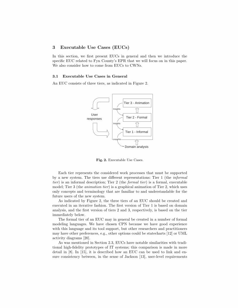
An EUC consists of three tiers, as indicated in Figure 2.

Tier 3 - Animation

Tier 2 - Formal

Tier 1 - Informal

Domain analysis

Insights

Insights

User responses

I n s i g h t s

Fig. 2. Executable Use Cases.

Each tier represents the considered work processes that must be supportedby a new system. The tiers use different representations: Tier 1 (the informaltier) is an informal description; Tier 2 (the formal tier) is a formal, executablemodel; Tier 3 (the animation tier) is a graphical animation of Tier 2, which usesonly concepts and terminology that are familiar to and understandable for thefuture users of the new system.

As indicated by Figure 2, the three tiers of an EUC should be created andexecuted in an iterative fashion. The first version of Tier 1 is based on domainanalysis, and the first version of tiers 2 and 3, respectively, is based on the tierimmediately below.

The formal tier of an EUC may in general be created in a number of formalmodeling languages. We have chosen CPN because we have good experiencewith this language and its tool support, but other researchers and practitionersmay have other preferences, e.g., other options could be statecharts [12] or UMLactivity diagrams [20].

As was mentioned in Section 2.3, EUCs have notable similarities with tradi-tional high-fidelity prototypes of IT systems; this comparison is made in moredetail in [8]. In [15], it is described how an EUC can be used to link and en-sure consistency between, in the sense of Jackson [13], user-level requirements

and technical software specifications. Jackson’s division into requirements andspecifications resembles the division into subtasks and solution proposals in taskdescriptions. User-level requirements and subtasks lie to the left of the dividingline in Figure 1; technical software specifications and solution proposals lie tothe right.

Like a task description, an EUC can have a broader scope than a traditionaluse case. The latter is a description of a sequence of interactions between externalactors and a system that happens at the interface of the system. An EUC can gofurther into the environment of the system and also describe potentially relevantbehavior in the environment that does not happen at the interface. Moreover,an EUC does not necessarily fully specify which parts of the considered workprocesses will remain manual, which will be supported by the new system, andwhich will be entirely automated by the new system. An EUC can be similar to,indeed, a task description. Therefore, Executable Use Cases do not necessarilyhave the most suitable name. The name “executable use cases” was originallychosen to make it easy to explain the main idea of our approach to people, whowere already familiar with traditional prose use cases.

3.2 Executable Use Case for Fyn County’s EPR

We have made an EUC that covers all seven task descriptions listed in thebeginning of Section 2.2. The EUC lies strictly on the left-hand side of thedividing line in Figure 1, i.e., the EUC does not include solution proposals.

In this section, we will present the part of the EUC that corresponds to thetask description of Table 1. The informal tier of the EUC is the task descriptionitself.

An extract of the formal tier is shown in Figure 3; this figure presents theCPN model that corresponds to the task description from Table 1. Note thatthis is only one of the seven task descriptions for Fyn County’s EPR.

Thick lines denote the path that the user and system has to complete tosolve the task; i.e. to go from the place Ready to make appointment to Patientready for arrival. Solid lines denote subtasks and variants of subtasks. Dashedlines denote added structure to the model to assert that desired interleavings ofsubtasks/variants are possible.

In Figure 4, we outline how the formal and animation tiers are related. Atthe bottom, we see the formal tier executing in CPN Tools. Please note thatthe shown module of the CPN model contains seven transitions (the rectangles),and that each of these transitions corresponds to one of the considered tasks(cf. the list in the beginning of Section 2.2). At the top is the animation tier inBRITNeY, the new animation facility of CPN Tools. The two tiers are connectedby adding animation drawing primitives to transitions in the CPN model. Theseprimitives update the animation.

The animation tier is a view on the state of, and actions in the formal tier.When a transition occurs in the formal model it is reflected by updates to theanimation tier. Therefore, the behaviors of the two tiers remain synchronized.

patient

patient

patient

patient

patient

patient

patient

patient

patient

patient

patient

patient

patient

patient

patient

patient

patient

patient

patient

patient

patientpatient

patient

patient

patient

patient

patient

Requestinterpreter

(5)

Deny request(4d)

Transfer case(4c)

Park task(4b)

Transfer towaiting list

(4a)

Go back 2

Printnotification

(4)

Appointmentmade

Goback 1

Continue 2

Possible clinicalsession

(3)

Consilidate plans(2q)

Adjust data(2a)

Transfer iincompatiable data

(2p)

Establishepisode of care

(2)

Continue 1

Security(1c)

Add companion(1b)

Patient exists(1a)

Register patient(1)

Intake

Finalizerequest

PATIENT

Establishing episode of

carePATIENT

Ready to makeappointment

In

PATIENT

Patientready forarrival

Out

PATIENT

Registeringpatient

PATIENT

Out

In

Fig. 3. Task 1 modeled in CPN

Using the animation tier the user can interact with each of the seven tasks.Within the animation of each task, subtasks can be selected and executed. Whena subtasks is chosen for execution, the animation user can see visually what ishappening and see which entities that are involved in completing the subtask.In the snapshot shown in Figure 4, the animation visualizes Task 1. It showsthat the animation user has chosen to execute subtasks 1, 3, 4, and is aboutto execute Subtask 4a. We also see that Subtask 4a involves a computer and asecretary.

Subtask 1 Subtask 3 Subtask 4 Subtask 4a

Fig. 4. Connection between animation and formal layer

In the task description in Table 1, it was not mentioned, who does what. It isus, the creators of the EUC (software people), who have interpreted the subtasksin this way, i.e., described who does what and what a normal execution of a taskis. When showing this animation to the staff at a hospital in Fyns County, we

are likely to get more feedback on our interpretations of their daily work thanwe could get with the static task descriptions only.

3.3 From Executable Use Cases to Colored Workflow Nets

The EUC we have presented above describes real-world work processes at ahospital. When these work processes are to be supported by a new IT system,of course, what goes on inside that system is highly related to what goes on inthe real world.

In the approach of this paper (cf. Figure 1), we make separate models ofreal-world work processes at a hospital (the EUC) and the IT system that mustsupport these work processes (the CWN). This is done to clearly distinguishbetween the real world, on one hand, and the software, on the other hand. Thisdistinction is advocated by a number of software experts, see, e.g., [13]. Notmaking this distinction may cause serious confusion.

In this way, the CWN we will now present describes the IT system, and, aswe will see, can be used to automatically generate parts of that system.

4 Colored Workflow Nets

A Colored Workflow Net (CWN) [3] is a CPN as defined in [17]. Although boththe CWN and the formal tier of the EUC use the same language, there aresome notable differences. First of all, the scope of the CWN is limited to theIT system, i.e., only those activities that are supported by the system appear inthe model. Second, the CWN covers the control-flow perspective, the resourceperspective, and the data/case perspective [4]. In the case study of this paper,the EUC covered the control-flow perspective only, but as we move to the rightin Figure 1, it is necessary to include the other perspectives as well (if theyhave not already been included). Finally, CWNs are restricted to a subset ofthe CPN language, i.e., CWNs need to satisfy some syntactical and semanticalrequirements to allow for the automatic configuration of a workflow managementsystem [3].

Although a CWN covers the control-flow, resource, and data/case perspec-tives, it abstracts from implementation details and language/application specificissues. A CWN should be a CPN with only places of type Case or Resource.These types are as defined in Table 2.

A token in a place of type Case refers to a case and some or all of its at-tributes. Each case has an ID and a list of attributes. Each attribute has a nameand a value. Tokens in a place of type Resource represent resources. Each re-source has an ID and a list of roles and organizational units. The distributionof resources over roles and organizational units can be used in the allocation ofresources. For more details on CWNs, we refer to [3].

Figure 5 shows the CWN for the task Request before patient arrives.When comparing this CWN with the EUC CPN shown in Figure 3, severaldifferences can be observed. First of all, some subtasks shown in the EUC CPN

Table 2. Places in a CWN need to be of type Case or Resource

colset CaseID = union C:INT;

colset AttName = string;

colset AttValue = string;

colset Attribute = product AttName * AttValue;

colset Attributes = list Attribute;

colset Case = product CaseID * Attributes timed;

colset ResourceID = union R:INT;

colset Role = string;

colset Roles = list Role;

colset OrgUnit = string;

colset OrgUnits = list OrgUnit;

colset Resource = product ResourceID * Roles * OrgUnits timed;

are not included in the CWN because they will not be supported by the ITsystem. Subtask 1b (Add companion) and Subtask 2q (Consolidate plans) arenot included because of this reason. Secondly, Figure 5 includes more explicitreferences to the resource and data/case perspectives. Note that Figure 5 showsthree resource places of type Resource defined in Table 2. These resource placeshold information on the availability and capabilities of people. Using the conceptof a fusion place [14, 27], these places together form one logical entity. Placesof type Case hold information on cases. Cases have several attributes such aspatient name, patient id, address, birth date, preliminary diagnosis,etc. In Figure 5, the relevant attributes are only shown for the task Registerpatient, but, for the sake of readability, not shown for all other tasks.

One of the advantages of using Petri nets is the availability of a wide varietyof analysis techniques. In CPN Tools it is possible to simulate models and to dostate-space analysis. We have used both facilities. For the state-space analysis wehave abstracted from time and color to asses soundness [4]. Initially, we discov-ered a minor error (a deadlock because we did not connect Subtask 4d properly).However, after repairing this, the CWN was sound. Note that reachability graphof the CWN shown in Figure 5 for one patient has only 14 nodes and 29 arcs,so it is easy to verify its correctness by hand. However, for more complicatedCWNs, automated state-space analysis of CPN Tools is indispensable to assescorrectness before implementation.

5 Realization of the System Using YAWL

In [3], it was shown that for some CWNs it is possible to automatically gen-erate BPEL template code [7]. The Business Process Execution Language forWeb Services (BPEL4WS or short BPEL) [7] is a textual XML based languagethat has been developed to form the “glue” between webservices. Although it isan expressive language, it tends to result in models that are difficult to under-

c_outc_in

r

r

r

r

r

r

r

r

r

r

c

c

c

c

c

c

c

c

c

c

c

c

c

c

c

c

c

Deny request(4d)

[has_role(r,"Secretary")]

Transfer case(4c)


Transfer towaiting list

(4a)


Printnotification

(4)


Appointmentmade

Goback 1

Continue 2

Clinical session(3)

Adjust data(2a)

Transfer incompatiable data

(2p)

Establishepisode of care

(2)

Continue 1

Patient exists(1a)


Register patient(1)


input (c_in);output (c_out);actionlet val c_out = set_att(c_in,"Patient Name") val c_out = set_att(c_out,"Address") val c_out = set_att(c_out,"Patient Id") val c_out = set_att(c_out,"Zipcode") val c_out = set_att(c_out,"City")in c_outend;

Intake

Resource 3

Resource

Resource

Resource

Resource 1

Resource

Resource

Finalizerequest

Case

Establishing episode of care

Case

Ready to makeappointment

In

Case

Patientready forarrival

Out

Case

Registeringpatient

Case

Out

In

Resource

Resource

resources



[has_role(r,"Doctor")]


c

c

Go back 2

c

c

Resource 2

ResourceResource

resources

resources

Fig. 5. CWN for the task Request before patient arrives

stand and maintain. For example, it is not possible to show BPEL code to endusers (e.g., to visualize management information or to allow for dynamic change[24]). Moreover, BPEL offers little flexibility and no support for the resourceperspective.3 Therefore, we decided to use YAWL [1] rather than BPEL.

YAWL (Yet Another Workflow Language) [1] is based on the well-knownworkflow patterns (www.workflowpatterns.com, [2]) and is more expressive thanany of the other languages available today. Because of its native and unrestrictedsupport of the deferred choice pattern [2], it is possible to leave the selection of

3 Note that only recently people started to investigate adding the resource perspec-tive to BPEL, cf. the WS-BPEL Extension for People (BPEL4People) initiativehttp://www-128.ibm.com/developerworks/webservices/library/specification/ws-bpel4people/.

the next task to the user. This offers more flexibility than BPEL, because it ispossible to define for each state what tasks are possible without selecting one (inBPEL this is restricted to the inside of a pick activity [7]). Moreover, YAWLalso supports the resource perspective (in addition to the control-flow and dataperspectives). The language YAWL is also supported by an open source workflowmanagement system that can be downloaded from www.yawl-system.com.

Fig. 6. Screenshot of YAWL editor

Given the fact that YAWL can be seen as a superset of CWNs, it was easy totranslate the running example from CPN in YAWL. Figure 6 shows the top-levelworkflow and the composite task Request before patient arrives. Althoughboth models look quite different, a fairly direct mapping was possible from theCWN shown in Figure 5 to the YAWL model shown in Figure 6. All places oftype Case in Figure 5 are mapped onto conditions in YAWL and transitions inFigure 5 are mapped onto YAWL tasks.4

After mapping the CWNs onto a YAWL specification, it is possible to enactthe associated workflows. Figure 7 shows a work-list and a form generated byYAWL. The left-hand side of the figure shows the work-list of the secretary withuser code secretary4. It shows work-items associated to three cases. Each ofthese three cases is in the state registering where three tasks are enabled.Therefore, there are 3*3=9 possible work-items. After selecting a work-itemrelated to task register patient, three work-items disappear from the work-

4 Note that subtasks in Task Descriptions correspond to transitions in CWNs andtasks in YAWL.

Secretary 4 selects a

work-item from her

worklist and start filling

out information of

patient Anne Jansen

Fig. 7. Screenshot of the YAWL worklist and the form associated to task register

patient

list (the competing tasks become disabled for this patient) and secretary4 canfill out a form with patient data. After completing the form there are again ninework-items, etc.

The realization of the workflow process in YAWL completes the overall ap-proach shown in Figure 1, i.e., we moved from informal task descriptions, thento EUCs, after that to CWNs, and finally realized the task descriptions in termsof YAWL. Note that, given the availability of a running YAWL system and aCWN, it is possible to construct a running system in a very short period, e.g., ina few hours it is possible to make the process shown in Figure 6 operational. Thisdoes include the generation of user forms as shown in Figure 7 but does not in-clude system integration or the development of dedicated applications. The taskof mapping a CWN onto YAWL can be partly automated by using the auto-matic translation provided by ProM (cf. www.processmining.org). ProM is ableto automatically map Petri nets in PNML format onto various other formats,including YAWL. However, this translation does not take data and resourcesinto account, so some manual work remains to be done. Nevertheless, it showsthat the overall process shown in Figure 1 is feasible. Moreover, we would like toargue that initially more time is spent on the requirements, but considerably lesstime is spent on the actual realization and testing. The intermediate steps (i.e.,EUCs and CWNs) enable an efficient implementation. Moreover, less time needsto be spent on testing the system because its design has been validated andverified earlier. Also, the system is more likely to be accepted by the end-users.

6 Related Work

This paper builds on the work presented in [3], where we also apply CPN Toolsto model EUCs and CWNs. However, in [3], EUCs are not linked to task descrip-tions and we used BPEL as target language instead of YAWL. The extensionwith task descriptions was inspired by the work of Lauesen [18, 19]. Comparedto existing approaches for requirements engineering and use case design [9, 11,13, 25], our approach puts more emphasis on the two intermediate steps. Firstof all, we make EUCs with both an animation and formal tier. Second, we useCWNs to link these EUCs to concrete implementations.

Today, workflow technology is used in areas such as radiology [26]. However,there is no systematic and broader support for workflows in health-care organi-zations. Vendors and researchers are trying to implement “careflow systems” butare often confronted with the need for more flexibility [22, 23]. The state conceptin CPN and YAWL (e.g., places with multiple outgoing arcs modeling a choicewhich is resolved by the organization rather than the system) allows for moreflexibility than classical workflow systems. We know of one other applicationof YAWL in the health-care domain. Giorgio Leonardi, Silvana Quaglini et al.from the University of Pavia have used YAWL to build a careflow managementsystem for outpatients. However, they did not use task descriptions, EUCs, andCWNs. Instead they directly implemented the system in YAWL.

7 Conclusions

In this paper, we realized a small careflow system using the four-step approachdepicted in Figure 1 and motivated the added value of each of the three transfor-mation steps in our approach. Obviously, the system made using YAWL is notthe full EPR for Fyn County. It is just a prototype illustrating the viability of ourapproach. To come from an extensive and detailed set of task descriptions — asthe seven task descriptions we have been considering — to their implementationrequires large amounts of work and extensive involvements of the stakeholders. Aweaknesses of the work presented in this paper is the unavailability of stakehold-ers in coming from the task descriptions to the EUC, the CWN, and the YAWLimplementation (stakeholders have been extensively involved in the writings ofthe task descriptions, but this is beyond the scope of this paper).

The language we used both for Executable Use Cases (EUCs) and ColoredWorkflow Nets (CWNs) is CPN. For the actual realization of the system we usedYAWL which can be seen as a superset of CPNs (extended with OR-joins andcancellation sets [1]) dedicated towards the implementation of workflows. Thestate-based nature of these modeling languages fits well with task descriptions,i.e., in a given state it is possible to enable multiple tasks and let the environmentselect one of these tasks. This is not possible in many workflow systems becausethere the system selects the next step to be executed.

Although CPNs and YAWL allow for more flexibility than classical workflowmanagement systems, we would like to argue that in the health-care domainmore flexibility is needed than what is provided by YAWL as it has been used inthis paper. Work on computer-interpretable guidelines [21] shows that classicalworkflow languages tend to be too restrictive. Health-care workers should beallowed to deviate and select alternative pathways if needed.

To conclude this paper, we would like to discuss three extensions to allow formore flexibility.

– Dynamic change. The basic idea of dynamic change is to allow for changeswhile cases are being handled [24]. A change may affect one case (e.g., chang-ing the standard treatment for an individual patient) or many cases (e.g., anew virus forcing a hospital to deviate from standard procedures). Althoughthis approach is very flexible, it requires end-users to be able and willing tochange process models.

– Case handling. Case handling [5] comprises a set of concepts to enablemore flexibility without the need for adapting processes. The basic idea isthat there are several mechanisms to deviate from the standard flow, e.g.,unless explicitly disabled people can skip and roll-back tasks. Moreover, thecontrol-flow perspective is no longer dominating, i.e., based on the availabledata the state is constantly re-evaluated and the collection and visualizationof data is no longer bound to specific tasks.

– Worklets. Worklets [6] allow for the late binding of process fragments, e.g.,based on the condition of a patient the appropriate treatment is selected.YAWL supports the uses of worklets, i.e., based on ripple-down rules an

appropriate subprocess is selected. The set of ripple-down rules and therepertoire of worklets can be extended on-the-fly thus allowing for a limitedform or dynamic change.

Each of these approaches can be combined with the four-step approach depictedin Figure 1. However, further work is needed to develop EUCs and CWNs thatcan capture the degree of required flexibility and link this to concrete workflowlanguages allowing for more flexibility. Currently, even the most innovative sys-tems support only one form of flexibility. For example, Adept [24] only supportsdynamic change, FLOWer [5] only supports case handling, and YAWL [6] onlysupports worklets. Hence, future work will aim at an analysis of the variousforms of flexibility in the context of the approach presented in this paper.

Acknowledgements We thank Søren Lauesen for permission to use the taskdescriptions for the Fyn County EPR as basis for this paper. We also thankSøren for fruitful discussions and feedback on this paper.

References

1. W.M.P. van der Aalst and A.H.M. ter Hofstede. YAWL: Yet Another WorkflowLanguage. Information Systems, 30(4):245–275, 2005.

2. W.M.P. van der Aalst, A.H.M. ter Hofstede, B. Kiepuszewski, and A.P. Barros.Workflow Patterns. Distributed and Parallel Databases, 14(1):5–51, 2003.

3. W.M.P. van der Aalst, J.B. Jørgensen, and K.B. Lassen. Let’s Go All the Way:From Requirements via Colored Workflow Nets to a BPEL Implementation of aNew Bank System. In Proc. of 13th International Cooperative Information SystemsConf., volume 3760 of LNCS, pages 22–39, Agia Napa, Cyprus, 2005. Springer.

4. W.M.P. van der Aalst and K. van Hee. Workflow Management: Models, Methods,and Systems. MIT Press, 2002.

5. W.M.P. van der Aalst, M. Weske, and D. Grunbauer. Case Handling: A NewParadigm for Business Process Support. Data and Knowledge Engineering,53(2):129–162, 2005.

6. M. Adams, A.H.M. ter Hofstede, D. Edmond, and W.M.P. van der Aalst. Facil-itating Flexibility and Dynamic Exception Handling in Workflows. In O. Belo,J. Eder, O. Pastor, and J. Falcao e Cunha, editors, Proceedings of the CAiSE’05Forum, pages 45–50. FEUP, Porto, Portugal, 2005.

7. T. Andrews, F. Curbera, H. Dholakia, Y. Goland, J. Klein, F. Leymann, K. Liu,D. Roller, D. Smith, S. Thatte, I. Trickovic, and S. Weerawarana. Business ProcessExecution Language for Web Services, Version 1.1. Standards proposal by BEASystems, International Business Machines Corporation, and Microsoft Corpora-tion, 2003.

8. C. Bossen and J.B. Jørgensen. Context-descriptive Prototypes and Their Applica-tion to Medicine Administration. In Proc. of Designing Interactive Systems (DIS)2004, pages 297–306, Cambridge, Massachusetts, 2004. ACM Press.

9. A. Cockburn. Writing Effective Use Cases. Addison-Wesley, 2000.10. Krav til Fyns Amts EPJ-system (udkast) — Requirements to Fyn County’s EPR

System (Draft). Fyns Amt, 2003.

11. P. Grunbacher, A. Egyed, and N. Medvidovic. Reconciling software requirementsand architectures with intermediate models. Software and Systems Modeling,3(3):235–253, 2004. Springer.

12. D. Harel. Statecharts: A Visual Formalism for Complex Systems. Science ofComputer Programming, 8:231–274, 1987.

13. M. Jackson. Problem Frames — Analyzing and Structuring Software DevelopmentProblems. Addison-Wesley, 2001.

14. K. Jensen. Coloured Petri Nets – Basic Concepts, Analysis Methods and PracticalUse. Vol. 1, Basic Concepts. Monographs in Theoretical Computer Science. AnEATCS Series. Springer, 1992.

15. J.B. Jørgensen and C. Bossen. Executable Use Cases as Links Between ApplicationDomain Requirements and Machine Specifications. In Proc. of 3rd InternationalWorkshop on Scenarios and State Machines (at ICSE 2004), pages 8–13, Edin-burgh, Scotland, 2004. IEE.

16. J.B. Jørgensen and C. Bossen. Executable Use Cases: Requirements for a PervasiveHealth Care System. IEEE Software, 21(2):34–41, 2004.

17. L.M. Kristensen, S. Christensen, and K. Jensen. The Practitioner’s Guide toColoured Petri Nets. International Journal on Software Tools for TechnologyTransfer, 2(2):98–132, 1998.

18. S. Lauesen. Software Requirements — Styles and Techniques. Addison-Wesley,2002.

19. S. Lauesen. Task Descriptions as Functional Requirements. IEEE Software,20(2):58–65, 2003.

20. OMG Unified Modeling Language Specification, Version 1.4. Object ManagementGroup (OMG); UML Revision Taskforce, 2001.

21. M. Peleg and et al. Comparing Computer-interpretable Guideline Models: ACase-study Approach. Journal of the American Medical Informatics Association,10(1):52–68, 2003.

22. S. Quaglini, M. Stefanelli, A. Cavallini, G. Micieli, C. Fassino, and C. Mossa.Guideline-based Careflow Systems. Artificial Intelligence in Medicine, 20(1):5–22,2000.

23. S. Quaglini, M. Stefanelli, G. Lanzola, V. Caporusso, and S. Panzarasa. Flexi-ble Guideline-based Patient Careflow Systems. Artificial Intelligence in Medicine,22(1):65–80, 2001.

24. S. Rinderle, M. Reichert, and P. Dadam. Correctness Criteria For DynamicChanges in Workflow Systems: A Survey. Data and Knowledge Engineering,50(1):9–34, 2004.

25. I. Sommerville. Software Engineering — Seventh Edition. Addison-Wesley, 2004.26. T. Wendler, K. Meetz, and J Schmidt. Workflow Automation in Radiology. In H.U.

Lemke, editor, Proceedings of Computer Assisted Radiology and Surgery (CAR98),pages 364–369. Elsevier, 1998.

27. CPN Tools. www.daimi.au.dk/CPNTools.

� �� ! "�$#�&%('*)+-,.�0/�� 1��2�34 )657 ��8,9+-) ;:��*�$�0)<=�>��-��/?��

@BADCFEHG8IKJLC�JLCKMONDADCKJQP�RKJLC�SUTWVXVWTWCFELPYADCZ�[]\_â`cbedgfihkjclmbedn\_l�oKpaq]rsptdndgferupaq_Z�dnpvbwfed

x paruyzdgfelwr{b|j�[0}~hc[]`tbe��iàlmbwf��0�ur�� n��lw[]p��]��dnliZ$�]\_â`tln�aht��0��k�D� x hc�$��i�7��

o~\-�0ru�W�t��c�z�0�v�z�z��k�0��v�z ]¡v�c��¢W�z¡t£z��¢� ��~¢��]�Q�K¤z¥�¡c�]��¦c��¡~¢X§t£�¨�¨v£�¡v©z�v¥0¡k�]�z¡c£z��ª¢� ]��~¢w�0�

«!¬ªn®n¯�°Q±�®�² �³p´ru\_^L[]fwb��0pkb�µ��Q��f��]µgbed¶ferslmberuµH[]} � [�·aru�ud¸��¹�º�[vµ�»idgb��[]fe�kl�¼ � �i»�o½�$l�¾¿rulÀf��]ârs¹c�ujµ¶�a�]ptq�rupaqÀbe[�^L[]�u[�q�rudnl-¹càd_be[¿be�ad-\_[�yzdn\_dgpkb�[0}��rufedg�sdglwl_\_[�·aru�ud!¹tdnykruµndnl8be�Q��b��d�lw�a�]�u��fedg}ÁdgfBbe[6�]lpa[k¹cdnlnÂ½�7f��¹cruberu[]pQ�]��fe[]`tberupaqÃ�]â^cfe[z�0µ¶�tdnl_µY�]ptpa[0b_·Ld�`tlwdY¹Ä¹cr{fednµgbe�{jHrupÄlw`tµ¶�Hdnpkykr{fe[�pa\_dgpkbelnÂF�$�c`tl_�pkà\B·Ld¶f�[0}�dgÅc^Ldgferu\_dnpvb��]��fe[]`tberupaq�^tfe[0be[vµn[��ul?�Q�Yyzd�·Ldndnp*¹tdnlwruq]padY¹�be[�lw`trub?be�td�ptdg�Æµn[]pQ¹tr{beru[�ptlnÂ�Ç�pad[]}Èbe�adnlwdirul�be�ad³É�jcpQ�0\_rsµ � �³»�o~�ÊÇ�ptË|¹cdn\-�]pa¹�¼ÌÉ³Í � Ç?¾Kfe[]`tberupaq�^tfe[0be[vµn[��D·LdnruptqB¹cdnyzdn�u[�^Ldn¹-·vj�be�ad��pvbedgfeptdgb�oKpaq�ruptdndgferupaqÀ��]lw�*Îa[]feµnd]ÂFZ�[]\_^Q�0fedn¹�be[¿[0be�adgf�[]ptË|¹tdg\-�]pQ¹¿fe[]`tberupaq¿^cfe[]be[vµn[]�uln�ªr{b�[�pt�uj�fedgËÏ àr{fednl$be�ad�\_[�lmb�·a�]lwruµ�fe[�`cbed?¹trulwµn[�yzd¶fwj��0pQ¹-\-�]rupvbednpQ�0paµnd�^tfe[vµndY¹c`tfednlnÂt��[B¹tdgbed¶fe\_rsptdi��tdgbe�adgf�be�tdgfed�0fedi�]pvjUlw`t·tbe�ud³dgfwfe[]fel½[]f�¹cdnlwruq�p_ÐL�n��ln�z��diµ¶fedY�0bed��Z�[��u[�`cfedY¹�Ñªd¶bwferQ»�dgbi¼XZ$ÑK»?¾~\_[k¹cdn�a[0}ÈÉ³Í � Ç��v�]lbe�ad�Òafelmb�lmbednÛbe[Y��f�¹tl�r{bel½yzdgfer{ÒQµY��beru[�p7Âc�$�td�\_[k¹tdn�t`tberu�ursÓgdnl��?µn[�\_\_[]pUpad¶b�lmbwfe`tµgbe`tfed��rube�U}Áàptµgberu[�palrupÀ�0feµ�dgÅc^tfedglwlwrs[]pal�fedn^tfedglwdnpvbersptqBbe�ad�fe[]`tberupaqU�]�uq�[0ferube�t\_lnÂL�$�trsl³µn[]\_\_[�pÀZ$ÑK»�â�0bwbedgfep¿µn�]p¿·Ld?`tlwdY¹be[�\_[k¹tdn�½[]be�ad¶fU[�pcË|¹tdn\-�0pQ¹6fe[]`tberupaq�^cfe[]be[vµn[]�sl�}Ô[]f � �i»�o~�$lnÂªÕÃd�¹c[�pa[]bB�0bwbedg\_^tb�be[�\_[k¹tdn�~be�adµ¶�a�]ptq�rupaq-be[�^L[]�s[]q]j�[0}½be�td�ptdgb��[]fe�À¹crufedgµgbe�{jv�L·a`cb�rupalmbedn��¹�\_[k¹tdn�Èbe�ad8pa[k¹td�fe[�`cberupaq-b��]·a�udnlnÂ7Ç�`cf�d¶ÅcË^Ldgferu\_dnpvbel�lw�t[��Öbe�Q�0b½be�arul�\_[k¹cdn�QµY�0p�lwru\�à�s�0bed�be�ad�fed Ï àr{fedY¹Ufe[�`cberupaq8[�^Ldgf��bers[]pal�¹cdgÒQptdY¹Urup!É�Í � Ç��]l��$dn�u�7�]l�be�ad?¹kjcpQ�]\_ruµY�0�u�uj!µ��Q�0paq�ruptqBbe[�^L[]�s[]q�rudnli[]}K� � �³»�o~��Â×�ØkÙ7Ú8Û ¯0Üª�Ý É�Í � Ç��aZ�[��u[]`tfedY¹ÀÑªdgbwferÈ»�d¶beln� � �³»�o~�$ln�a\_[k¹cdn�u�sruptq_�]pa¹�lwru\B`t��beru[�p7�ayzdgfer{ÒQµn�0beru[�pÈÂ

Þ ßtàiáLâDã?ä8å8æ�áDç�ã³à

èêé ALë~TWVÌì è M¸í�A�î�ï!ìvP¶ð�ALñ0ò´ó é�è ï�ô8õ�ö!÷ÔøQùmútû�TWü�JLÇJLIFPYADCFADýHADIKü�ü�þ�üYPYìký(ALÿ�ý�ALë~TXVÌì-CFAªMFìkü��gP8MFA�ìküCFALP?IKüYì_JLC7þ��Kñ0ìvì��ªTWü�P�TWCFE¿TWCFÿ�ñ0JLüYPYñ0IKîzP�IKñ�ì�JLCKMÃP�RFìvñ0ìUTXü�CKA¿îzìkC7PYñ0JLVWT�vìkM�JLMKýHTWCKTXüYPYñ0JQP�TÌADC�aõ-RFìUCFìvP�ðBALñ�òPYA��$ADVÌALELþýHJkþ�î0R~JLCFELì-ñ0J��~TXMKVÌþ�JQP�IKC �~ñ�ìkMKTWîzP�JQë~VWì�P�TWýHìküvùLMKIFì_PYAÀP�RFì-JQñ�ë½TÌPYñ0JQñ�þÃý�A��Lìký�ìkC7P8ALÿ�CFAªMFìkü��õ-RFì��~IKñ��$ADüYì�ALÿ�P�RFì��nCÈPYìvñ]CFìvP!ô8CKEDTWCFìvìvñ0TWCKE*õ�JLüYò��FALñ0îzìÄó��nô8õ��ö é�è ï�ô8õ��"ALñ�ò�TXCFE��ñ�ADI � ó��6ö÷ÔøLø�ûBTXü¿PYAOüYP�JLCKMKJQñ]MKT��vì�� ñ�ADIFP�TWCKE �~ñ�ALPYA�îzADVXüÀP�RKJQP6JQñ�ìÄü�IKTÌPYìkM�PYA�ð�TÌñ�ìkVÌìkü�ü¿JLMÆRKA�îìkC!��TWñ�ADCKý�ìkC7P�ü��"�ì��Lìvñ0JLV�ñ�ADIFP�TXCFE#�Kñ�ALPYAªîzADVWü�÷%$7ùQø�&Fù�'�(�ù)'�*tûÀRKJ)�Lì´ë$ìvìkC>MFì��LìkVWA��ìkM>ë7þ P�RKTXü+��ÃùBP�RFì�VWJQPYìkü�P¸ë$ìkTWCFEP�RFì-,�þªCKJLýHTWî é�è ï�ô8õ/.¿C 0�MFìkýHJLCKM ó1,UG é .�öÖñ�ADIFP�TXCFE2�~ñ�ALPYA�îzADVÄ÷3*tûeù-J CFìvð ñ�ìkJLîzP�T��LìÆñ0ADIFP�TWCFE�Kñ�ALPYAªîzADV4� �nCÊñ�ìkJLîzP�T��Lì*ñ�ADIFP�TWCFE��Kñ0ALPYA�îzADVWükùFñ�ADIFPYìkü-JQñ�ìÀADC~VÌþÄMKTXü�îzA��Lìvñ�ìkM�ð!RFìkCÊP�RFìvþ JQñ�ì�CFìvìkMKìkMÆómT4�{ì��5�687:9<;�=+>�6?9 ö]ù8J@�Lìvñ�þ�MKTBA$ìvñ�ìkCÈPJ��8�Kñ0ADJLî0R PYA"P�RKJQP�IKüYìkM�ë�þ îzADC!�LìkCÈP�TWADCKJLVDC �ªìkM�CKìvP�ðBALñ�ò ñ0ADIFP�TWCFE�Kñ�ALPYAªîzADVWü��8,_G é .�ADC~VÌþ¸ñ�ì)E�IKTÌñ0ìküUP�RFì6ý�ADüYP_ë½JLü�TWî¿ñ�ADIFPYì*MKTWü�îzAF�Lìvñ�þÖJLC~M�ýHJLTWC7PYìkCKJLCKîzìG�~ñ�A�îzìkM~IFñ�ìküvùë~JLüYìkM6ADC*J�ü�TWý+�½VWT�CKìkM¿îzADý*ë~TWCKJQP�TÌADC6ALÿFP�ðBA��Kñ�ì��ªTÌADIKü�ñ�ìkJLîzP�T�Lì�ñ�ADIKP�TWCFE��Kñ0ALPYA�îzADV!�Kñ�AªîzìkMKIFñ�ìkü�÷Ôø�&Fù�'�*tûH�õ-RFñ0ìvì-TWý+�~VÌìkýHìkCÈP�JQP�TÌADC~ü�ALÿI,_G é .1÷Ôø)*�ù4'�Jªù4(�Jaû$RKJ��Lì!ë$ìvìkCHJLCKCKADIKCKîzìkM�÷Ôø�Jaûeù7JLC~MHüYADý�ì��~ñ�ìkVWTWýHTXCKJQñ�þñ�ìkü�I~VÌP�üEDT��LìkC TWCê÷Ôø)'tûH�8õiAÆMFìvPYìvñ0ý¸TWCFìÊð!RFìvP�RFìvñ�P�RKìvñ�ì�JQñ�ìOü�IKëKP�VÌìÖìvñ�ñ�ALñ0üALñ¸MKìkü�TÌEDCLK~Jcð!üvù?ÿ�ALñ0ýHJLV�Lìvñ0T�C½îvJQP�TÌADC ALÿ¿P�RFì�A��$ìvñ0JQP�TÌADC~üHALÿ¿P�RFìM�Kñ0ALPYA�îzADV-TXüHCFìkîzìkü�ü�JQñ0þ ÷3(�'tûH�Uõ-RKTXü��~J��$ìvñN�Kñ�ìküYìkC7P�üHJOCKñ0üYPJQPYPYìký+�KP�TWC P�RKTWü*MKTÌñ�ìkîzP�TÌADC ë7þ"ÿ�ALñ0ýHJLVXTWü�TWCFE P�RKìÖMFþªCKJLýHTXî�A��$ìvñ0JQP�TÌADCKü*ALÿP,UG é . IKü0TWCFE´@BADVWADIFñ�ìkM��ìvPYñ0T�ï�ìvP�ü*óe@D��ï�ü�öÀ÷Ôø)(�ù]ø)QtûH��nCN�Kñ0ì��TÌADI~ü�ð�ALñ�òO÷3(�$cûeù7ð�ìR�Kñ�AF��TWMKìkMHJLÇJQë~ü�PYñ0JLîzPU@D��ï�ý�A�MKìkVFALÿ�JG�Kñ�ADJLîzP�T�LìP�Kñ�ALPYAªîzADVwùDòªCFAtð!C

JLüUP�RFìG,�ìküYP�TWC~JQP�TÌADCS0�"�ì)E�IFìkCKîzìkMT,¿TWüYP�JLCKîzì�0HU?ìkîzPYALñ�V-ADIKP�TWCFE�ó1,G"S,WU�öX�Kñ�ALPYAªîzADV�÷3'�QtûH�Y��ñ�ADJLîzP�T�Lì��Kñ�A�0PYAªîzADVWü8JQPYPYìký+�~P8PYA6ìkü�P�JQë~VWTWü�R�JLC~MHýHJLTWC7P�JLTWC�ñ�ADIKPYìkü8JLü8ü�A7ADCÄJLü�P�RFìvþ�JQñ�ì!JLîzP�T�aJQPYìkMÖTWCP�RFì éOè ï�ô�õÀù

ñ0JQP�RFìvñ�P�RKJLCZC~C~MKTWCFE�ñ�ADIFPYìkü�ADCMFìkýHJLCKM�Qõ-R�IKü�P�RFìBñ�ADIFP�TWCFE¿ý�ìkî]RKJLCKTWü�ý¸ü³ALÿ[,�" ,WU JLCKM�,UG é .�JQñ�ì�Lìvñ�þ¸M~TBA�ìvñ0ìkCÈP��!�"ì¿M~TWü�îvIKü�ü�ìkM�P�RFì¿VWTÌPYìvñ0JQP�IFñ0ì!ñ�ìkVWJQPYìkMÄPYAý�A�MKìkVWVWTWCFE�R~TÌEDRKVÌþ�MFþªCKJLýHTWî!üYþ�ü�PYìkýHü�I~ü�TWCFE@D��ï�ü_TWC"÷3(�$cûH�~SBñ0TWì�KKþLù ��TXCKMKVÌAtð JLCKM SUTWVXVWTWCFELPYADC�÷3\tû³IKüYìkM í�TÌEDRS0^]³ì��LìkV�iìvPYñ]T�ï!ìvP�ü6÷3(tû�PYAHýHA�MFìkV$MFþ!0CKJLýHTXî!MKTWC~TWCFE��~RKTXVÌADüYA��~RFìvñ]üvùLð!RKTWî]RHADCKVWþHîzADCKü�TWMFìvñ]ü8JÃîvTÌñ0îvIKVWJQñ�PYA��$ADVÌALELþ��!_¿TÌADCFEÃìvPUJLV4��÷3(�(�ùH(`&QûiRKJ��Lì�Kñ�ìkü�ìkCÈPYìkM J�P�TWý�ìkM @D��ï&ý�AªMFìkVBÿ|ALñP�RFì è MS0�RFAªîT.¿C 0�MFìkýHJLCKML,¿TWüYP�JLCKîzìTU?ìkîzPYALñ�ó è .�,WUÀöñ�ADIFPa0TWCFEb�Kñ�ALPYAªîzADVB÷3'`&QûH�,¿IFì6PYAÖP�RFìc��ìvñ]îzìkT��LìkM�M~T�d¸îvIKVÌP¶þÄALÿ�ý�A�MKìkVWVWTWCFE�JQñ�ë½TÌPYñ0JQñ�þ î0R~JLCFEDTWCFEÄPYA��ADVWALEDTÌìküvù_¿TÌADCFE�ìvP�JLVH�tADCKVWþ�îzADCKü�TWMFìvñ�JLC�J��8�Kñ0A)�FTWýHJQP�TÌADC�èÀñ0TWü�PYìkCKüYìkC*ìvP�JLV�÷Ôøkútû~RKJ��LìUI~üYìkMRKTÌìvñ0JQñ0î]RKTWîvJLVª@D�8ï�üPYA�ý�A�MKìkV éOè ï�ô8õ-ü��õ-RFìÄCFìvP�ðBALñ�òÆPYA��$ADVÌALELþÆTWü*MKTÌñ�ìkîzP�VWþ�ýHA�MFìkVXVÌìkM�ù�ë~IFP*CFAOñ�ADIKP�TWCFEM�Kñ0ALPYA�îzADVBTWüîzADCKü�TXMFìvñ�ìkM�Lõ-RFìkÇTWC�÷Ôø�$cûeùÈP�RFì-ô�MFELìPV!ADIFPYìvñf,¿TWü�îzAF�Lìvñ�þN��ñ�ALPYAªîzADV~TXü?ý�A�MKìkVWVÌìkMJLCKMHJLCKJLVWþ�üYìkMg�!"ªTWýHTB0VWJQñ0VWþLù½÷Ôø)\tû�ý�A�MKìkVWü�P�RFì�TWC7PYìvñ�A��$ìvñ0JQë~TWVWTWP�þZ�Kñ�ALPYAªîzADVwùÈë�þ�ð!RKTWî]RN�~JLî0òLìvP�üDKKAcð ë$ìvP�ðBìvìkCÊJ6îzALñ�ì¿CFìvP�ðBALñ�òJLCKMHJLÇJLMHRFAªî_CFìvP�ðBALñ�ò��TXJ¿P�RFì-îvVÌADüYìküYP8EDJQPYìvðBJcþ¸îzADCKCFìkîzP�TWCKEÀP�RFì-P�ðBA6CFìvP¶ð�ALñ0ò�ü��7õ-RFì-MFþªCKJLýHTWîvJLVXVÌþî0R~JLCFEDTWCFE�PYA��$ADVÌALEDTWìkü�ALÿ$P�RFì!ìkC7P�TÌñ�ì�CFìvP�ðBALñ�òHJQñ�ì!CKALP�îzADCKü�TXMFìvñ�ìkM��nCHîzADC7PYñ0JLüYPvù�ADIFñ8ðBALñ�òÿ|AªîvIKüYìkü8ADCý�AªMFìkVWVWTXCFEHP�RFìñ�ADIFP�TXCFE��~ñ�ALPYA�îzADV�TWC�MFìvP�JLTXVwù�JLC~M�ì��S�Kñ�ìkü0ü�TWCFEÖP�RFìMFþ�C~JLýHTWîvJLVWVÌþ�î]RKJLCFEDTWCKEÖPYA��$ADVÌALELþ�ªTWJ6I ��MKJQP�TXCFEÀñ�ADIFP�TWCKE6P�JQë~VÌì�ìkCÈPYñ]TÌìkü��ªô8JLî0RÊCFAªMFì�I ��MKJQPYìkü8TÌP�ü�ñ�ADIFP�TXCFE�P�JQë~VÌì�ë�þHîzñ�ìkJQP�TWCFEFùªI ��MKJQP�TWCFEALñ¿TWC<�QJLVWTWM~JQP�TWCFE�P�RFìÃñ�ADIFPYì*ìkCÈPYñ0TWìküvù½JQÿ�PYìvñ¿ñ�ìkîzìkT��ªTWCFE¸P�RKìc,UG é . îzADC7PYñ�ADV�ý�ìkü�ü�JQELìkü¿PYñ]JLCKü�ýHTÌPYPYìkM�TWCP�RFì6ü�þ�üYPYìkýM�~õ-R�IKüvùFP�RFì�ñ0ADIFPYì�ìkC7PYñ0TÌìküvùKîzADC7P�JLTWCFìkM�TWCÊP�RFì6CFAªMFìÀñ�ADIKP�TWCFE�P�JQë~VÌìkükùKñ�ìkîzALñ0M P�RKì6îvIFñ�ñ�ìkC7PîzADCKCFìkîzP�TWADCOë$ìvP�ðBìvìkCĆFA�MKìküvùKð!RKTXî0R ñ�ì�K~ìkîzP�ü!P�RFì6PYA��ADVWALELþ ALÿ?P�RFì6CFìvP¶ð�ALñ�ò�VÌìkJQñ0CFìkM ÿ�ñ�ADý P�RFì��ªTÌìvðALÿ?CFAªMFìküvùFJLü!TWü_MKADCFì6TWC Jñ�ìkJLV éOè ï�ô�õ��

õ-RKìÖýHJLTXC�JLTXý ALÿ!P�RKTWüZ�~J��$ìvñÃTXü*PYA�ì��ªPYìkCKM P�RFì ý�AªMFìkVWVWTXCFEOJ��8�Kñ0ADJLî0R MFì��LìkVÌA��$ìkM TWC�÷3(�Qtûeù?ë7þ�Kñ�AF��TXMKTWCFE-JÀ@D�8ï ýHA�MFìkV7ALÿKJ�RKTÌEDRKVÌþÀMFþªCKJLýHTXî éOè ï�ô8õÀùað!TÌP�R*CFA�MKìkü³ñ0I~CKCKTWCFE�,_G é .Z�`�"ìBìkýN�~VÌAcþJ�ELìkCFìvñ]TWî�CFìvP!ü�PYñ0IKîzP�IFñ�ì�ü0IKTÌPYìkMÊPYAÄýHA�MFìkVXVWTWCFEÃñ�ìkJLîzP�T��Lìc�Kñ�ALPYAªîzADVWü-TWCÊELìkCFìvñ]JLV4�~õ-RFì*ü:�$ìkîvT�C~îvüUALÿ�P�RFì,UG é . ñ0ADIFP�TWCFEÃJLVÌELALñ0TÌP�RKý¸ü�JQñ�ì¿P�RFìkCÄñ�ìkJLVWTXüYìkM¸ë�þHÿmIKCKîzP�TÌADC~ü8TWCÄP�RFì¿JQñ0î�ì��h�Kñ0ìkü�ü�TÌADCKü8ALÿ³P�RFì¿ý�AªMFìkV4��"ìHJLVWüYAÊîzADCKü�TXMFìvñÀüYADý�ìA��KP�TWýHT�kJQP�TÌADCÁ��ìvñ]JQP�TÌADCKü�ALÿX,UG é .Ãù�ü�IKî]R´JLüÀJLCÁLñ0TWEDTWCKJQPYALñÀCFAªMFìÃI~ü�TWCFEJLC ;�i�jS>�6?9�kl6!m@nok�6!m�p);�>�n:q�r ómüYìvì�"�ìkîzP�TÌADC-'Dö�PYA üYìkJQñ]î0R"ÿ�ALñÀñ�ADIFPYìkü¿PYA P�RFì�MFìkü�P�TWCKJQP�TÌADC��TWCKJLVXVÌþLù~ðBìJLVWüYAs�$ìvñ�ÿ|ALñ]ý.üYADý�ìÖü�TWýÃIKVWJQP�TÌADCÆì��h�$ìvñ0TWýHìkCÈP�ü6PYA´MFìkýHADCKüYPYñ0JQPYìÄP�RFìÄðUJkþ P�RFìÄý�AªMFìkV�îvJ��KP�IFñ�ìkü*P�RFìMFþªCKJLýHTWî¿î]RKJLCFELìkü�TWC CFìvP�ðBALñ�òÊPYA��$ADVÌALELþ��

õ-RKìvñ�ìÆJQñ�ìÆüYì��Lìvñ0JLV6îzADCÈPYñ0TWë~IFP�TÌADCKüÖALÿÃP�RKTWüT�~J��$ìvñ)�W��TÌñ0ü�P�VÌþLùUÿ|ADVWVWAcð!TWCKE�ADCêÿ|ñ�ADý;ADIKñ��Kñ�ì��ªTÌADIKüðBALñ�ò ÷3(�Q�ùo(�$cûeù�ðBìÖýHA�MFìkV�P�RFìÊMFþªCKJLýHTWîvJLVWVWþ´î]RKJLCFEDTWCFE´PYA��$ADVÌALEDTÌìkü*ALÿ é�è ï�ô8õ-üÃñ0I~CKCKTWCFE ñ0ìkJLîzP�T��Lìñ�ADIFP�TXCFEM�Kñ�ALPYAªîzADVWüÃTWCKîvVWI~MKTWCFEÊý�ìkü�ü�JQELì VÌADü0ü6JLCKM ñ�ìvPYñ0JLCKü�ý¸TWü�ü�TÌADCg�t"�ìkîzADCKMKVÌþLùið�ì��Kñ�AF��TWMKìHP�RFì CKñ0üYPÿ�ALñ0ýHJLV�ü:�$ìkîvT�C~îvJQP�TWADCÊALÿ³P�RFìG,UG é . ñ�ADIFP�TXCFE��Kñ�AªîzìkMKIFñ�ìkü��Fõ-R~TÌñ0MKVÌþLù7ð�ì�M~TWü�îzA��Lìvñ�TWCKîzALñ�ñ�ìkîzP_ñ0ADIFP�TWCFETWCFÿ�ALñ0ýHJQP�TWADC*TWCÃP�RFìUñ�ADIKPYìUM~TWü�îzA��Lìvñ0þ��Kñ�AªîzìkMKIFñ0ì�MKIFìUPYAÀJLý*ë~TÌEDIFADIKü�üYP�JQPYìkýHìkCÈP�ü�TWC6P�RKìUü��ìkîvTC~îvJQP�TÌADC÷3*tû�ë�þÄü�TWýÃIKVWJQP�TWADCÄì��S�$ìvñ0TWý�ìkC7P�ü��S��TWCKJLVWVÌþLù�ðBì�ü�IFELELìküYP-ý�AªMKT�C½îvJQP�TÌADCKü�PYA�P�RFìG,UG é .u�~ñ�A�îzìkM~IFñ�ìküUTWCJLC�JQPYPYìký+�~P!PYAHAF�Lìvñ0îzADý�ìÃP�RKTWüD�Kñ�ALë½VÌìký��

õ-RKì ñ�ìküYPHALÿ¿P�RFìM�½J��ìvñHTXü�ALñ�EDJLCKTWü�ìkM JLüHÿ�ADVWVÌAtð!ü��X"�ìkîzP�TÌADCv'"MFìkü�îzñ]TÌë$ìküP�RFì�ë~JLü�TXîÊA��ìvñ]JQP�TÌADCKüALÿX,_G é .Z��nCO"�ìkîzP�TÌADC#(�ù�ð�ì+�~ñ�ìküYìkC7P�ADIKñ�@W�8ï1ýHA�MFìkViALÿD,UG é .Z�t"ªTXý*IKVXJQP�TÌADCOì��S�$ìvñ0TWý�ìkC7P�ü¿JQñ�ìîzADCKMKI~îzPYìkM"TWCw"ªìkîzP�TÌADCw& JLCKM"MKTWü�îvI~ü�üYìkM´TWCw"ªìkîzP�TÌADC-*h��TXCKJLVWVÌþLù$îzADCKîvVWIKü0TÌADCKü�JLCKM�ÿ�IKP�IFñ�ìÃð�ALñ�ò´JQñ�ì�Kñ�ìkü�ìkCÈPYìkM�TXCx"�ìkîzP�TÌADCsQh�

y zw{�à}|~�ç�æO��#�O�+��Oà��zäf�Y~v|�à8ä��ã³å�áLç¶à}��¸âDã�áLã?æªã��nCÄP�R~TWü�ü�ìkîzP�TÌADC�ùªð�ì��Kñ0ìküYìkCÈPBP�RFì¿ë~JLî0ò7ELñ�ADI~CKMÖALÿt,UG é . TXCÄP�RKìRCKìkVXM¸ALÿiñ�ADIFP�TWCFEÃJLVÌELALñ0TÌP�R~ýHü��ªõ-RFìkCP�RFìë~JLü�TXî6A��$ìvñ0JQP�TÌADC~ü�ALÿ�,UG é . JQñ0ìMKìkü�îzñ0TÌë$ìkM�ë7þ´JÖü0TWý+�~VÌì*ì��ªJLýN�~VÌìÃP�RKJQP�TWVWVWI~üYPYñ0JQPYìkü�P�RFìñ�ADIFPYìMKTWü0îzA��Lìvñ�þ JLCKM ýHJLTXCÈPYìkCKJLC~îzìG�Kñ�AªîzìkMKIFñ�ìkü)�

�I�4� �Z�Y�F��?�F�[�t�t�,¿TWüYP�JLCKîzìW�LìkîzPYALñ�ñ�ADIFP�TWCKE¿JLVWELALñ0TÌP�RKýHü_÷3'�'tû½JQñ0ì_ë~JLüYìkMADC�P�RFì_ü�RKALñ�PYìküYP��~JQP�R�îzADý+�½IFP�JQP�TÌADCHJLVÌELALñ]TÌP�RKý�Kñ�ìkü�ìkCÈPYìkMÖë�þHS�ìkVXVWýHJLC�÷3'tûH�ªõ!RFìRV!ADIFP�TWCFEZ�gCKÿ|ALñ0ý¸JQP�TÌADCb�8ñ�ALPYA�îzADV?ó1VP��Uö�÷3'ªø�û�TWüBJÃü�TWý+�~VWì!JLCKM��Kñ0JLîo0

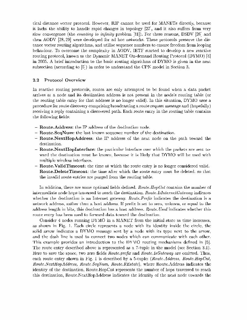
P�TWîvJLV?MKTXüYP�JLCKîzìZ�LìkîzPYALñ��Kñ�ALPYAªîzADV4��í�AcðBì��LìvñkùtVP�� îvJLCKCKALPÀë�ìIKüYìkM�ÿ�ALñ éOè ï�ô8õ-ü�M~TÌñ�ìkîzP�VÌþLù�ë$ìkîvJLIKüYìTÌP�VWJLî0ò�ü¸P�RFì�JQë~TWVWTWP�þÆPYAÆRKJLC~MKVÌìÊñ0J��~TWM î]RKJLCFELìkü¸TXC PYA��$ADVÌALELþ ÷3'�$cûeù�JLC~M TÌP�JLVWüYAÆü�ISA$ìvñ0üÿ�ñ�ADý��Lìvñ�þü�VÌAtð1îzADC!�Lìvñ�ELìkCKîzì´ó�P�RKì q 5�¡S6Y¢1k�6!m@¢H5skl6�£}68k1¢1¤ �~ñ�ALë~VÌìký ÷3(ªø�û�ö¥�t�KALñ6P�RFìküYì¸ñ�ìkJLüYADCKüvùg,G"S,�U ÷3'�QtûUJLCKMP�RFìkC è .�,WU ÷3'Lú�ù�'�\tûBðBìvñ�ìÄMKì��LìkVÌA��$ìkMÆÿ�ALñ*JLM�RFA�î¸CFìvP�ðBALñ�òªü��õ!RFìküYìN�Kñ0ALPYA�îzADVWüc�Kñ�ìkü�ìvñ��LìHP�RFìÖMKTWüa0P�JLCKîzì��LìkîzPYALñ�ñ�ADIFP�TWCKE¿JLVWELALñ0TÌP�RKýHükùaJLCKM�IKP�TWVWTWüYìUüYì)E�IFìkCKîzì-C�IKý*ë�ìvñ]üiPYAÀìkC~ü�IFñ�ìUÿ�ñ�ìvìkMFADý ÿ�ñ�ADý VÌA�A��~TWCFEë$ìkRKJ)�ªTÌADIFñ��õ³A�A��Lìvñ0îzADý�ìÖP�RFìÖîzADý+�~VÌì��FTÌP�þ"TWC è .�,WUÃùt�nô8õ��üYP�JQñ0PYìkM PYA´MFì��LìkVÌA�� J�CFìvð1ñ0ìkJLîzP�T��Lìñ�ADIFP�TXCFEG�Kñ�ALPYAªîzADVwùDòªCFAtð!C¸JLü�P�RFìR,�þªCKJLýHTWî éOè ï�ô�õ¦.ÀCS0�MFìkýHJLCKMbV-ADIFP�TWCKE��ñ�ALPYAªîzADV�ó1,UG é .�ö�÷ &QûTWCw'�J�J�*h� è ëKñ]TÌìvÿ�TWC7PYñ�A�M~IKîzP�TÌADC�PYAÖP�RKìÃë½JLü�TWî*ñ�ADIFP�TWCFEÖJLVÌELALñ0TÌP�R~ýHü�ALÿf,UG é . TXü!EDT��LìkC"TXCOP�RFì�CFì��ªPü�IFë½üYìkîzP�TÌADCÆómJLîvîzALñ0MKTXCFEHPYA�÷3*tû�ö-TWCÊALñ0MFìvñ-PYAÄIKCKMFìvñ0ü�P�JLCKMÖP�RFìÃ@D��ï ý�AªMFìkV�TWCx"ªìkîzP�TÌADCx(h�

�I�§� ¨G�F�Y©��[ªR«�¬[!�F¬�®�<¯�nC ñ�ìkJLîzP�T��Lì´ñ�ADIFP�TXCFE#�Kñ�ALPYAªîzADVWüvù�ñ�ADIFPYìküÖJQñ�ìOADCKVWþ JQPYPYìkýN�KPYìkM>PYA�ë$ì�ÿ�ADIKCKM ð!RKìkC>J M~JQP�J-�~JLî0òLìvPJQñ�ñ0T�Lìkü6JQPJOCFAªMFì¸JLCKM TÌP�ü6MKìküYP�TWCKJQP�TÌADC JLMKMFñ�ìkü0ü�TWü6CKALP��Kñ�ìkü�ìkCÈPÃTWC"P�RFìÖCFA�MKì�°uü�ñ�ADIFP�TXCFE�P�JQë~VÌì�ó�ALñP�RFìñ�ADIFP�TXCFE¸P�JQë~VWìÃìkC7PYñ�þ�ÿ�ALñÀP�RKJQPÀJLMKMFñ0ìkü�ü�TXü�CKAÖVÌADCKELìvñ��aJLVWTXM½ö¥�Y�nC´P�RKTWü�ü�TÌP�IKJQP�TÌADC�ù[,UG é . IKüYìküÀJ�Kñ�AªîzìkMKIFñ0ì�ÿ�ALñ³ñ0ADIFPYì8MKTWü0îzA��Lìvñ�þ¿îzADý+�Kñ0TXü�TWCFEUëKñ�ADJLM~îvJLüYP�TWCFE-J_ñ0ADIFPYì�ñ�ì)E�IFìküYP³ýHìkü�ü�JQELì8JLCKMÄómRFA��$ìvÿ�IKVXVÌþFöñ�ìkîzìkT��ªTWCFEÃJ�ñ�ì��½VÌþHîzADCÈP�JLTXCKTWCFEÃJ6MKTWü0îzA��Lìvñ�ìkM �~JQP�R�ªô8JLî]RÖñ�ADIFPYì!ìkC7PYñ�þ¸TXCHP�RFì�ñ�ADIFP�TWCKE�P�JQë~VÌì¿îzADCÈP�JLTXCKüP�RFì�ÿ�ADVWVÌAtð!TWCFEZCKìkVWM~ü�±

²�³ �?��©�?��´ �µ�t�`h¶)¶ ±~P�RKì�� JLMKMFñ�ìkü�ü-ALÿiP�RFì*MFìküYP�TWCKJQP�TWADC CFA�MKì��²�³ �?��©�?�l·h¸¹s�µº ±FP�RFì*VWJLüYP_òªCFAcð!COüYì)E7IKìkCKîzì6C�IKý6ë$ìvñ_ALÿ�P�RFì6MFìkü�P�TWCKJQP�TÌADC�²�³ �?��©�?�B¹s<»©F¼x�Y½�´ �t�µ�`!¶)¶ ±-P�RFìw�� JLMKMFñ�ìkü0üÄALÿÃP�RFìÆCFì��ªP�CFAªMFì�ADC�P�RFì#�~JQP�R�PYAtðBJQñ0M P�RFìMFìkü�P�TWCKJQP�TÌADC�

²�³ �?��©�?�B¹s<»©F¼x�Y½µ¾)�[©�h�F¿À�8�� ±~P�RFìZ�~JQñ�P�TXîvIKVWJQñ�TXCÈPYìvñ�ÿmJLîzìÃA��Lìvñ¿ð!RKTWî]R�P�RFìZ�~JLî0òLìvP�üÀJQñ�ìÃü�ìkCÈP�PYA�0ðUJQñ0M�P�RFìHMFìkü�P�TWCKJQP�TÌADC"ýÃIKüYPÀë$ìò�CKAcð!C�ù$ë$ìkîvJLIKüYìHTWP¿TXüÀVWTÌòLìkVÌþ�P�R~JQPG,UG é . ð�TWVWVië�ì�IKü�ìkM�ð!TÌP�RýÃIKVÌP�T��½VÌì�ð�TÌñ�ìkVÌìkü�ü_TXCÈPYìvñ�ÿmJLîzìkü��

²�³ �?��©�?�ÂÁG�?ª�®��Ãc®1º2!�[�g© ±FP�RFì�P�TWý�ì�JQP!ð!RKTWî]RÊP�RFì�ñ�ADIFPYìÀìkC7PYñ�þ TWü_CFAÄVÌADCFELìvñ!îzADCKü0TWMFìvñ�ìkMT�QJLVWTWM�²�³ �?��©�?�BÄ�Sª�<©FhÃZ®1ºOh�?��© ±$P�RFì�P�TWý�ìHJQÿ�PYìvñ�ð!R~TWî0R�P�RFì�ñ0ADIFPYì�ìkCÈPYñ0þ´ýÃIKüYPÀë$ì�MFìkVÌìvPYìkM�ù�ü�A P�RKJQPP�RFì*TWC<�QJLVWTWMÖñ�ADIKPYìÀìkCÈPYñ0TWìkü-JQñ�ìG�~IKñ�ELìkMÊÿ|ñ0ADý�P�RFì�ñ�ADIKP�TWCFEP�JQë~VÌì��

�nC JLMKMKTÌP�TWADC�ù7P�RKìvñ�ìÀJQñ�ì�üYADý�ìÀA��KP�TWADCKJLV[CKìkVWMKüUMFì�C~CKìkM�YÅ 5�¡ ¢^;)ÆBÇ�5oj�Èµ6Y¢ îzADC7P�JLTWCKüUP�RFì�C�IKý*ë$ìvñBALÿTWC7PYìvñ0ý�ìkMKTXJQPYì-CFA�MKìURKA��~ü�PYñ0J)�Lìvñ]üYìkMHPYA�ñ0ìkJLî0R�P�RFì�MFìküYP�TWCKJQP�TWADC�<Å 5�¡ ¢^;)ÆBÉ p:É¥6Y¢^;�n¥6I;�¢�ÊW>�¢^;�Ëf>�¤ TWC~MKTWîvJQPYìküð!RFìvP�RKìvñÃP�RKì�MFìküYP�TWCKJQP�TWADC TWü�JLCÌ�nCÈPYìvñ]CFìvP�EDJQPYìvðBJcþ��DÅ 5�¡S¢^;�ÆÂÍWn:;4£ti TXCKMKTWîvJQPYìküÃP�RFì�MFìkü�P�TWCKJQP�TÌADC�TWü�JCFìvP¶ð�ALñ�ò�JLM~MFñ�ìkü�üvùFñ]JQP�RFìvñ!P�RKJLC�J¸RFADü�P!JLMKMFñ�ìkü0ü��8�gÿt�Kñ0ì�C �ÊTXü-üYìvP!PYA��vìvñ�AFù½I~CFòLAcð!C�ùKALñ!ì)E�IKJLV�PYAÄP�RFìJLMKMFñ0ìkü�üUVÌìkCFELP�RÊTWCÖë~TÌP�üvù�P�RKTWüUMFìkü�P�TWCKJQP�TÌADCÊRKJLüUJ�RFADüYP_JLMKMKñ�ìkü�ü��8Å 5�¡ ¢^;)Æ Îtp�;�9 TWCKMKTWîvJQPYìküBð!RKìvP�RFìvñUP�RKTWüñ�ADIFPYì6ìkCÈPYñ�þÊRKJLü_ë$ìvìkC�I~üYìkM PYAHÿ�ALñ�ðUJQñ0M�MKJQP�J�PYAtðBJQñ]M�P�RFì�MFìkü�P�TWCKJQP�TÌADC�

@BADC~ü�TWMFìvñ�& CFAªMFìkü¿ñ0IKCKC~TWCFEb,UG é .�TWC�J éOè ï�ô8õ�ÿ�ñ�ADý P�RFì�TWCKTWP�TWJLViü�P�JQPYìHJLüÀP�TWý�ì�TWCKîzñ0ìkJLüYìküvùJLü�ü�RKAcð!CêTXCv��TÌE �*ø��-ô8JLî0R îvTÌñ0îvVÌì�ñ�ì��~ñ�ìküYìkC7P�ü�J CFAªMFì"ð!TÌP�R�TÌP�ü�TXMFìkCÈP�TWP�þ TXCKü�TWMFì´P�RFìÆîvTÌñ]îvVÌìLù_P�RFìüYADVWTXM JQñ�ñ0Acð TWCKMKTXîvJQPYìküÖJL,UG é .=ý�ìkü�ü�JQELìÆüYìkC7PÊë7þ J�CKA�MFì´ð!TÌP�R TÌP�üÖP�þh�$ì"CFì��PÊPYA P�RFì�JQñ�ñ�Atð�ùJLCKM>P�RFìOMKJLü�R>VWTWCFì�TWü¸IKüYìkM PYA�îzADCKCFìkîzPÄP�ðBA CFAªMFìküHð�RKTWî0R>îvJLC>îzADýHýÃIKCKTWîvJQPYì�ð!TÌP�R ìkJLî]R>ALP�RKìvñ)�õ-RKTXü¸ì��FJLý+�~VÌì@�Kñ�AF��TXMFìküÄJLC�TWC7PYñ�AªMKIKîzP�TÌADC PYA P�RFìw,UG é .=ñ�ADIKP�TWCFE ýHìkî0RKJLCKTXü�ýHüÊMFì�C~CFìkM TWC ÷3*tûH�õ-RFì�ñ0ADIFPYì�ìkCÈPYñ0þ�MKìkü�îzñ0TÌë$ìkM�JQë$A��Lì¸TWü¿ñ0ì��Kñ�ìküYìkC7PYìkM JLü�J@$�0eP�I �~VÌìHTWC�P�RKìHý�A�MKìkV-ómüYìvì "�ìkîzP�TÌADC2(h�Wøcö¥�í�ìvñ�ì6PYAÖü�J)�LìÃP�RFì*ü��~JLîzìLù~P¶ð�A �vìvñ�AbC~ìkVWMKüRÅ 5�¡S¢^;�Æ j[n:;4£ti JLCKM@Å 5�¡ ¢^;)ÆBÉ p�ÊW>�¢^;�Ëf>�¤ JQñ0ì6ADýHTÌPYPYìkMg�½õ-R�IKüvùìkJLî0R ñ�ADIFPYì¸ìkCÈPYñ�þÆü0RFAcð!C TWC-��TÌE �8øÄTWü�MFìkü�îzñ]TÌë$ìkM�ë7þ"Jx*F0eP�I �½VÌì�±�óHÅ 5�¡ ¢^;�ÆÂÏR9�9�n�;op¥p Ð Å 5�¡ ¢^;)ÆBÇ�5oj�Èµ6Y¢�ÐÅ 5�¡ ¢^;�ÆÂÑZ;�i<¢§Ç�5¥j8ÏP9�9�n:;�p p Ð Å 5�¡ ¢^;�ÆÒ[; Ó¥ÑG¡S=cÐ Å 5�¡ ¢^;)Æ Å�Ô p�¢H>�¢^; ö]ù�ð!RFìvñ0ìNV-ADIFPYì�� è MKMFñ�ìkü0ü�TWCKMKTXîvJQPYìküÀP�RFìTWMFìkC7P�TÌP¶þ ALÿ8P�RFìMFìküYP�TWC~JQP�TÌADC�ù?V!ADIFPYì��uí�A��@UC7P�ñ0ì��Kñ�ìküYìkC7P�ü!P�RKìC�IKý*ë$ìvñ!ALÿ8RFA��½ü!PYñ0J��Lìvñ0üYìkM�PYAÊñ�ìkJLî]RP�RKTWü�MFìküYP�TWC~JQP�TÌADC�ù8V-ADIKPYì��uï!ì��ªP�í!A�� è MKMKñ�ìkü�ü¿TWCKMKTXîvJQPYìkü_P�RFì*TXMFìkCÈP�TWP�þÊALÿ?P�RFì*CKì��P!CKA�MFì6PYAcðUJQñ0MKü�P�RFì

MFìküYP�TXCKJQP�TÌADC�ùIV-ADIFPYì��Õ"ªì)E7ï�IKý9TWü�P�RFìHVXJLüYP¿ò�CFAtð!C"üYì)E�IFìkCKîzìHC�IKý*ë�ìvñ¿ALÿ�P�RFìHMFìküYP�TWC~JQP�TÌADC´ALñZÖ ;�na5 TWÿP�RKTWü�TWü¿IKCFòªCFAtð!C�ù½JLC~MsV!ADIFPYì��%V!ô�üYP�JQPYì¸TWü�üYìvP¿PYA kl68×�>�ØÂk19 TÌÿ?P�RKì�V!ADIFPYì��3U�JLVWTWM~õ-TWý�ìvADIFP¿TWü�ì��ªîzìvìkMKìkMJLCKM ×�>�ØÂk19 ALP�RFìvñ�ð!TWü�ì��

é ALñ�ìvA��Lìvñcù½PYA��Kñ�ìküYìkC7P!JHîzADý+�½VÌìvPYìG�~TWîzP�IKñ�ìÀALÿ�P�RFì6üYþªüYPYìký ùKðBì*JLü0ü�IKý�ìÀP�RFì*TWCKTÌP�TWJLV�ü�P�JQPYì6ALÿ�P�RFìé�è ï�ô8õ(TWC#��TÌE �8øDónøcö6TWü¿P�RKJQP�±³ÿ�ALñ�ìkJLî]R CFAªMFìLù�P�RKìvñ�ì¸TWü¿ADCFìÄñ�ADIFPYìHìkC7PYñ�þ�PYAOTÌP�ü�ìkVÌÿ¶ù�TXC�ð!RKTWî]R"P�RFìMFìküYP�TXCKJQP�TÌADC"JLCKM P�RFìHCFì��ªP6RFA�� JQñ�ìÄTÌP�üYìkVÌÿgù�P�RFì¸C�IKý*ë�ìvñÀALÿ_RFA��½ü�TWü�JLü�ü0TÌEDCFìkM"JLü�Jªù�JLCKMÆTÌP�ü6TWCKTÌP�TWJLVüYì)E�IFìkCKîzì6C�IKý*ë$ìvñ-TWü_JLü�ü�IKýHìkM PYAHë$ìHøHómü�TWCKîzìÀP�RKì6üYì)E�IFìkCKîzì6C�IKý*ë�ìvñ�J¸TWüUñ�ìküYìvñ��LìkMOJLCKM�TWü-I~üYìkMÊPYAñ�ì��Kñ0ìküYìkCÈP-JLC�IKCFòªCFAcð�C üYì)E7IKìkCKîzì�C7I~ý6ë$ìvñ�ö¥�

(1) initial state of four nodes.

4

2

1

3

(2,0,2,1,valid)(4,0,4,1,valid)

(1,0,1,1,valid)

(3,0,3,1,valid)

RREQ :(msg−type=RREQ, hoplimit=3, hopcnt=0,

4

3

1

RREQ

RREQ

2

(4) node 1 sends another RREQ;nodes 3 and 4 receive it.

(1,0,1,3,valid)

(2,0,2,1,valid)

NumAddrs=2, AddTarget=2, AddOrig=1,SeqOrig=3)

(4,0,4,2,valid)(1,1,1,2,valid)

(3,0,3,2,valid)(1,1,1,2,valid)

2

4

1

3RREP

(4,0,4,4,valid)(1,1,1,3,valid)(2,1,2,2,valid)

(3,0,3,3,valid)(1,1,1,3,valid)


(1,0,1,3,valid)

2

4

1

3RREP


(3,0,3,3,valid)(1,1,1,3,valid)



4

RERR3

2

1

RERR

(4,0,4,4,valid)(1,1,1,3,valid)(2,1,2,2,invalid)

(1,0,1,3,valid)(2,2,4,2,invalid)(4,1,4,4,valid)

(3,0,3,3,valid)(1,1,1,3,valid)

it; node 3 broadcasts a RREQ, node 1 receives it.

4

1

3

RREP


2(2,0,2,2,valid)(4,1,4,3,valid)(1,2,4,3,valid)

(4,0,4,3,valid)(1,1,1,3,valid)

which processes it.(6) node 2 unicasts a RREP to node 4,

which processes it.(7) node 4 unicasts a RREP to node 1,

(2,2,4,2,valid) is the route entry required.(8) node 1 processes the RREP,

node 1 and 3 receive it.(9) node 4 broadcasts a RERR,

NumAddrs=2, AddTarget=1, AddOrig=2,

RERR :(msg−type=RERR, hoplimit=3, hopcnt=1,NumAddrs=1, UnreaAdd1=2, SeqAdd1=2)

2

4

3

1 RREQ

(5) node 4 broadcasts a RREQ, node 2 and 1 receive

(1,0,1,3,valid)

SeqOrig=3, Seq1=3)

RREQ :(msg−type=RREQ, hopl=2, hopcnt=1,NumAddrs=3, AddTarget=2, AddOrig=1, Add1=3,


(3,0,3,3,valid)(1,1,1,3,valid)

SeqOrig=3, Seq1=3)

RREQ :(msg−type=RREQ, hoplimit=2, hopcnt=1,NumAddrs=3, AddTarget=2, AddOrig=1, Add1=4,

RREP: (msg−type=RREP, hoplimit=3, hopcnt=0,


(4,0,4,1,valid)

4

3

1RREQ

2

(2) node 1 broadcasts a RREQ;nodes 3 and 4 receive the RREQ.

(1,0,1,2,valid)

(3,0,3,1,valid)

(2,0,2,1,valid)

NumAddrs=2, AddTarget=2, AddOrig=1,SeqOrig=2)

2

4

3

1

so does node 3, because the hoplimit contained

(1,0,1,2,valid)


(3,0,3,2,valid)(1,1,1,2,valid)

SeqOrig=2, Seq1=2)

in the message is not greater than 1.

(3)node 4 discards the processed RREQ,

NumAddrs=3, AddTarget=2, AddOrig=1, Add1=3,

SeqOrig=2, SeqTarget=3, Seq1=4, TarHop=2)

RREP: (msg−type=RREP, hoplimit=2, hopcnt=1,NumAddrs=3, AddTarget=1, AddOrig=2, Add1=4,

SeqOrig=2, SeqTarget=3, TarHop=2)

RREQ

1−3

1

1

1 RREQ :(msg−type=RREQ, hoplimit=0, hopcnt=1,NumAddrs=3, AddTarget=2, AddOrig=1, Add1=4,SeqOrig=2, Seq1=2)

1−4


1

1

1

RREQ

RREQ

1−4

1−4

1−4

1−3

1−3

4

4

4

Ù�ÚÕÛ ²�ÜQ² ��lwru\_^t�sd?d¶Åa�0\_^a�ud�[0}K��fe[�`cbed�¹trulwµn[�yzdgfwj��0pQ¹�\-�0rspvbednpa�]ptµnd�^cfe[vµndY¹t`cfed?[]}KÉ�Í � Ç

è ü�ü�IKýHì�P�RKJQPÄCKA�MFì øOCFìvìkMKüÄJÆñ�ADIKPYìOÿ�ALñÄCFAªMFìs'h�X�¶PÄëKñ�ADJLMKîvJLüYP�üÖJÆñ0ADIFPYì�ñ�ì)E�IFìküYP�ó1VPV!ôDÝ�öý�ìkü�ü0JQELì��½õ-RFìcVPV!ôDÝ ý�ìkü�ü0JQELì*ÿ�ALñ0ýHJQP*÷3*tû�TWü_EDT��LìkC�TWCM��TÌE �?'Fónøcö¥� è VPV�ô�Ý�ýHìkü�ü�JQELì*îzADC7P�JLTWCKü�JLCÉ:ÍÞÇc; >�9<;�n ù³Jxß ;op¥p�>)mh;ZÇZ;�><9<;�n ù³JLC ÏR9�9�n�;op¥p�àPØB5)q�á JLCKM J îzALñ�ñ�ìkü:�$ADCKMKTXCFE ÏP9�9�n:;�p pb¢1ØÂ×�7�â�Ø�5)q�á ómT4�{ì��ã è MKMFñ�ìkü�ü!õ�]�U¿ü�äHTWCx��TWE �?'FónøcöYö6÷3QtûH��õ-RFìG�a�>í�ìkJLMFìvñ�ALÿ?JNVPV�ô�Ý�îzADC7P�JLTWCKü!P�RFìG�a� ü�ADIFñ0îzì6JLMKMKñ�ìkü�üómCFALP�ü�RKAcð!C�TWC+��TÌE �<'FónøcöYö]ù�JLCKMP�RFìW�a�ÆMFìküYP�TXCKJQP�TÌADC�JLMKMFñ0ìkü�ü_ó É:Í�ÆBåZ;�po¢1k�6?>�¢1k45�6hÏR9�9�n�;op¥p ö]ù�ð!RKTWî]R�TWü�üYìvP

ResvResv

(1) Example IPv4 RREQ Message

0 1 2 3 4 5 6 7 8 9 0 1 2 3 4 5 6 7 8 9 0 1 2 3 4 5 6 7 8 9 0 1

IP Header

msg−hopcnt

msg−size

0

: Unreachable.Addr (cont)

Resv 0 10

HeadLength=0

msg−tlv−block−size = 0

Unreachable.Addr :

Message Header

Address Block

(2) Example IPv4 RERR Message

0 1 2 3 4 5 6 7 8 9 0 1 2 3 4 5 6 7 8 9 0 1 2 3 4 5 6 7 8 9 0 1

msg−hopcnt

msg−size


Target.Tail

Orig.SeqNum

Orig.Tail

0

: size

Resv 0 1

0

0

1 0 0 Index Start=1 Index Stop=1

Message Header

Address Block

Address TLVs

Head :

msg−size


: size=7

Resv 0 1

0

0

1 0 0

Message Header

Address Block

Address TLVs

IP Header

0Number Addrs=2

msg−hoplimit

TLV−blk−size=0

: Head (cont)

HeadLength

TLV−blk−size :

tlv−type:DYMOSeqNum

msg−hoplimit

Number Addrs=1

msg−type:RERR

msg−type:RREQ

tlv−length=16

IP.DestinationAddress=ALL_MANET_ROUTERS

IP.DestinationAddress=ALL_MANET_ROUTERS

ÙgÚÂÛ ²�æÈ² É³Í � Ç´\_dnlwle�]q]d�}Ô[]fe\-��bel

PYA Ïèç�ç ß ÏRÑ Ô�é Å�ê Î éÔfÅ Ò ù³TWCKM~TWîvJQP�TWCFEÊP�RKJQP6JxVPV!ôDÝ�TWü¿ë~ñ�ADJLMKîvJLüYPÃTWC�P�RFì é�è ï�ô8õG��nC"P�RFìé ìkü�ü�JQELì�í�ìkJLMFìvñkù7P�RFì =Zpam�7�¢1¤¥j ; CKìkVWM�TXü�üYìvP�PYAÃü:�$ìkîvTÌÿ|þÃJGVPV�ô�Ý�ýHìkü�ü�JQELì�ëÈP�RKì =Zpam�7Àp�;�=N>�6Y¢1k4q�p CKìkVWMTWü�MKì�C~CFìkMÆJLüÖó1ìGí�î�ïYð�JSð�JSðkøcö]ù�ð!RKTWî]RÆTWCKM~TWîvJQPYìküÀP�RKJQP =cp:m�7Àrh5¥j?ØÂk�=Zk1¢ JLC~M =Zpam�7^rh5ojSq�6Y¢ JQñ�ìÄTXCKîvVWIKMFìkMTWC P�R~TWü-ý�ìkü�ü0JQELì�ë½JLCKM =cp:m�7Àp¥k Ö ; ü:�$ìkîvT�CKìkü_P�RKì6ü�T��vì�ALÿ?P�RKì�ìkCÈP�TWñ�ì6ý�ìkü�ü0JQELì*îzADIKC7PYìkM�TXC A�îzPYìvP�üó�ìkJLî0RúÃë~TÌP�ü�ö¥�h�nCÖP�RFì�üYìkîzADCKM VXTWCFì�ALÿiP�RFì é ìkü�ü�JQELì6í�ìkJLMFìvñkù~P�RFìÀýHüYE�0�RFA��~VXTWýHTÌP�ñ�ì��Kñ�ìküYìkC7P�üUP�RFì�ýHJ`�FTWýÃIKýC�IKý6ë$ìvñÊALÿ*RKA��~üÖA��LìvñOð�RKTWî0R�J ý�ìkü�ü0JQELìÆð!TWVWV!ë$ì´PYñ]JLCKü�ýHTÌPYPYìkMgë�P�RFìÆý¸üYE�0�RFA��îvCÈP TWC~MKTWîvJQPYìküÖP�RFìC�IKý6ë$ìvñ�ALÿ-RKA��~ü6J�ý�ìkü�ü�JQELìÊRKJLü*PYñ0J)�Lìvñ0ü�ìkM��õ!RFì =Zpam�7�¢1ØÂ×�7�â�Ø�5)q�á`7^pok Ö ; C~ìkVWMÆTWü*üYìvP6PYAwJªùiTWC~MKTWîvJQP�TWCFEP�RKJQP³JP,UG é .>ý�ìkü�ü�JQELì8MKA7ìkü�CKALP³îzADCÈP�JLTXC�P�RFì8ýHìkü�ü�JQELì�P�V��!0eë~VÌAªî�ò�ó�ðBì�MFìkü�îzñ]TÌë$ì�P�RKì?P�V��<0eë½VÌA�î0ò�VXJQPYìvñ�ö¥�ï�ì��Pvù~VXTWCFìkü�&�PYA�QÃALÿ��TWE �Y'Fónøcö_TWü_JLC ÏR9�9�n�;op¥pèàPØB5)q�á ùKð�RKTWî0R TXü_Jë~VÌAªî�ò¸ALÿ�JLMKMFñ0ìkü�üYìkü-JQë$ADIFPUð!RKTXî0RP�RFì¿ALñ0TÌEDTXCKJQPYALñ_ALÿ³P�RFìÀý�ìkü0ü�JQELì�ð!TWü0RFìkü8PYAHîzADC!�Lìvþ TWCFÿ�ALñ0ýHJQP�TÌADCg�7õ-RFì ÑG¡S=Nâ¥;�nPÏR9�9�n¥p TWC~MKTWîvJQPYìküBP�RFìC�IKý6ë$ìvñ?ALÿ$JLMKMFñ�ìkü0üYìkü�îzADC7P�JLTWCFìkMHTWCP�RKì-ý�ìkü�ü�JQELì��!�gC+,UG é .êý�ìkü0ü�JQELìküvùÈJLMKMKñ�ìkü�üYìkü�îzADC7P�JLTWCFìkM¸TWC�JLCJLMKMFñ0ìkü�ü8ë½VÌA�î0òHü�RKJQñ�ì�P�RFì¿ü�JLý�ì Çc; >�9 JLCKMÖRKJ)�Lì¿MKTBA$ìvñ�ìkC7P+é >�k�Øñp ��õ-R�IKüvù7P�RFì Çc; >�9�ç�;�6!m�¢�r ñ0ì��Kñ�ìküYìkC7P�üP�RFì!VWìkCFELP�R�ALÿ$P�RFì-ÿ�ADVWVÌAtð!TWCFE ÇZ;�>�9 CKìkVWM��RFìkCHîzADCKîvJQPYìkC~JQPYìkMÄPYA6P�RFì!í�ìkJLM�ù�é >�n4m!;�¢HÆ é >�klØ ñ0ì��Kñ�ìküYìkC7P�üP�RFì��a� JLM~MFñ�ìkü�ü?ALÿ$P�RFì�õiJQñ�ELìvPBMFìküYP�TWC~JQP�TÌADCHCFAªMFì-TWCKM~TWîvJQPYìkM�TWC+VPV�ô�ÝÃùtê n¥k�m<Æ é >�klØ ñ�ì��Kñ0ìküYìkCÈP�ü�P�RFì��a�JLMKMFñ0ìkü�ü_ALÿ?P�RFì�ALñ]TÌEDTWCKJQPYALñ�ALÿ�P�RKìcVPV�ô�ÝZ�Dé çfò�7:â�Øñá`7^pok Ö ; TWC P�RKì6JLMKMFñ�ìkü0ü-ë~VÌAªî�ò TWC~MKTWîvJQPYìkü_P�RFì6PYALP�JLVVÌìkCFELP�R"ómTWCÖAªîzPYìvP�ü]öBALÿiP�RFìÀTWýHý�ìkMKTXJQPYìkVÌþHÿ�ADVWVÌAcð�TWCFE6P�V�$ómü]ö]ùFCKJLýHìkVÌþÄõ�þ!�$ì�0^]³ìkCFELP�RS0HU�JLVWIFìHómõ�]<UÀö¥� è Cè MKMFñ�ìkü�ü!õ�]�U�ü:�$ìkîvT�CKìkü!üYADý�ì*JQPYPYñ]TÌë~IFPYìÈómü]ö]ù½ð!RKTWî]R�JQñ�ì6JLü0üYA�îvTXJQPYìkMOð!TWP�R�JLMKMFñ�ìkü0ücó�ìkü]ö_îzADC7P�JLTWCFìkM�TWCP�RFìM�~ñ�ìkîzìkMKTWCFE JLMKMFñ�ìkü�üHë~VÌAªî�ò[� è üÄü�RFAtð!C>TWCó��TWE �X'Fónøcö]ù�P�RKì ¢1ØÂ×�7a¢1¤ j8; TXüHüYìvP¸PYA å�ô ßõê Ò[; Ó¥ÑG¡S= �õ-RKTXü8ý�ìkJLCKü�P�RKJQPUP�RKTWü�JLMKMFñ�ìkü0ü8P�V��HîzADC7P�JLTWCKüBP�RFì¿üYì)E�IFìkCKîzì¿C7I~ý6ë$ìvñ8ALÿiüYADý�ì¿JLMKMFñ�ìkü�ütó�ìkü]ö�TWÿ�òªCFAtð!C�õ-RFì ¢1ØÂ×�7Àp�;�=N>�6Y¢1k4q�p TWü�MFì�C½CFìkMÆJLüÄó1ìGíFî)ï?ðkø�ð�JSð�JSð�JÈö]ù�TWCKMKTXîvJQP�TWCFEÊP�RFìHìkVÌìkýHìkCÈP�ü*TWCKîvVWIKMKìkM"TWC�P�RFìHP�V��ë~VÌAªî�ò�JQñ�ì�± k�6?9<; i�7Àpo¢H>�n�¢ ù k�6?9<;�i�7^p�¢H5¥j ù ¢1ØÂ×�7�Ø;�6!m<¢�r JLCKM ×`>�ØÕ¡Y; ��õ!RFì TWCKMFì��h0�üYP�JQñ�PHJLCKM TXCKMFì��h0�üYPYA�� JQñ�ìIKüYìkM PYA ü:�$ìkîvTÌÿ�þ P�RKìOJLMKMFñ�ìkü0üYìkü�ð!RFADü�ìOüYì)E�IFìkCKîzì�C�IKý*ë$ìvñ0ü�JQñ�ì�îzADC7P�JLTWCFìkM TWC P�RKTXü�P�V��[�8õ-RFì P�V��!0VÌìkCFELP�R�ü��ìkîvTCKìkü�P�RFì-ü�T��vì_ALÿ�ìkJLî0RÄüYì)E�IFìkCKîzì-C�IKý6ë$ìvñ�îzADC7P�JLTWCFìkM�ùDJLC~M+�aJLVXIFì_TWCKMKTWîvJQPYìUP�RFìkü�ì!üYì)E�IFìkCKîzìC�IKý6ë$ìvñ0ü)�<�nC��TÌE � 'Fónøcö]ùFP�RFì¿TWCKMFì��h0�üYP�JQñ�PBJLCKMÊTWCKMFì��h0�üYPYA��ÊJQñ�ì�ë$ALP�RÖüYìvPUPYAÖøQùFTWC~MKTWîvJQP�TWCFE6P�RFì�ü�ìkîzADCKMJLMKMFñ0ìkü�üNê nokBm!Æ é >�k�Ø TWCT�~ñ�ìkîzìkMKTWCFEHJLM~MFñ�ìkü�ü_ë½VÌA�î0ò½ùFð�RFìvñ�ìÀP�RFì�CKñ]üYP-JLMKMFñ�ìkü0ü�é >�n1mh;�¢HÆ é >�k�Ø TWü_TWC~MKTWîvJQPYìkMë�þè�vìvñ0A �tí�ìkCKîzìLùtP�RKì8üYì)E�IFìkCKîzì�C�IKý*ë$ìvñ�ALÿFP�RFì�ALñ0TÌEDTXCKJQPYALñiCFAªMFìGê nokBm!ÆÒI;�Ó¥ÑG¡S= ùkð!TÌP�RÀP�RKì8ü�T��vì8MKì�C~CFìkMJLü-P�V�<0�VÌìkCKELP�R�ùKTWü_TWCKîvVXIKMFìkM�

è üÊü�RFAcð�C TWC��TÌE ��øDó4'Dö]ù_CFAªMFì�øOëKñ0ADJLMKîvJLüYP�üÊJOVRV!ô�Ý.ý�ìkü�ü0JQELì ó�ñ0ì��Kñ�ìküYìkC7PYìkM�JLü ì�ì�ö�÷Zø]öJLCKM>P�RFìkC ðUJLTÌP�üHÿ�ALñÄJ ñ�ì��~VÌþ�� è PÄP�RKTWü¸P�TWý�ìLù�ADCKVWþ�CFAªMFìkü ("JLCKMù&�JQñ�ìOTWC ñ0JLCFELìOALÿÀCFAªMFì ø�JLCKMñ�ìkîzìkT��Lì�ì�ì�öZ÷�ø��7õiAÃTWC7PYñ�AªMKIKîzì_P�RFì�ñ�ADIFP�TXCFEG�Kñ�AªîzìkMKIFñ0ìkü�ü�TWý+�½VÌþLùDP�RFì�ý�ìkü�ü�JQELì�ADCKVÌþ�îzADC7P�JLTWCKüBýHJLTWCTWCFÿ�ALñ0ýHJQP�TWADC ð!TÌP�RFADIKPHîzADCKü�TWMFìvñ]TWCFEÆTÌP�üÄîzADCKîzñ�ìvPYì�MKJQP�J üYPYñ]IKîzP�IFñ�ìLù8JLC~M ìkVÌìký�ìkC7P�üÖîzADCKîzìvñ0CFìkM>ð!TÌP�R

p¥k Ö ; ALñ Ø�;�6!m�¢�r JQñ�ì�TWEDCFALñ�ìkM��õ-RFìTì�ì�öZ÷�øTWüü�RKAcð!C TWCÌ��TÌE �_øDó4'Dö¥�8õ-RFìÊP¶þ!�$ìÊALÿ!P�RFì ý�ìkü0ü�JQELì�TWüüYìvP�PYA2Å�ÅPÔ�úUù?P�RFì rh5¥j q�6Y¢ TXü�üYìvP�PYA-Jªù�JLCKM�P�RFì�TWCKTWP�TWJLV rS5¥j?ØÂkl=�k1¢ TWüüYìvP�PYA øQù�JLîvîzALñ0MKTXCFE"PYA"P�RFì;�i�jS>�6?9�kl6!mùn¥k�6!mÌp);�>�n:q�r MKìkü�îzñ0TÌë$ìkM TWC è .�,WU;÷3'�*tûeùBð�RKTWî0R TWüHPYAÌ�Kñ�ì��LìkC7PÊIKCKCFìkîzìkü�ü0JQñ�þ CFìvP�ðBALñ�ò!0ð!TWMKì6MKTWü�ü�ìkýHTWCKJQP�TÌADCÊALÿXVPV!ôDÝ¿ü��~ï�AªMFìÖø*TWCKîzñ�ìkýHìkCÈP�ü�TÌP�ü!ü�ì)E7IFìkC~îzìÃC�IKý*ë�ìvñ�ë7þ ADCKìLù�JLCKM�üYìvP�ü�P�RFìALñ0TÌEDTXCKJQPYALñÀJLMKMFñ�ìkü�ü�ó ÏR9�9 ê nokBm ö�JLCKM�üYì)E�IFìkCKîzìHC�IKý6ë$ìvñ�ó Ò[;�Ó ê n¥k�m ö!PYA�TÌP�ü�Atð!Cw�aJLVXIFì��S�ìkîvJLI~üYì�P�RFìüYì)E�IFìkCKîzì6C�IKý*ë$ìvñ_ALÿ�CFAªMFì�'�ó ÏR9�9 é >�n4m!;)¢ ö-TWü_I~CFò�CKAcð!C�ùFTÌP-TXü-CFALP-TWCKîvVXIKMFìkMÊTWCÊP�RFì6ýHìkü�ü�JQELì��nC+��TÌE �KøDó4(Dö]ù7CFAªMFìkü}(¿JLCKMN&��Kñ�Aªîzìkü�ü�P�RFì_ñ�ìkîzìkT��LìkMbVPV!ôDÝÃùLð!RFìvñ0ìBP�RKì-RFA��~VWTWý¸TÌPiTWü?MKìkîzñ�ìký�ìkC7PYìkM

ë�þ>ADCFìÆJLCKM�P�RKìÆRFA��îvCÈP TWüÊTWCKîzñ0ìký�ìkCÈPYìkM�ë�þ ADCFì��-õ-RFìkC ìkJLî0R CFAªMFì"îzñ�ìkJQPYìküOJ ñ�ADIKPYì´ìkC7PYñ�þ PYACFAªMFì�ø��?õiA�ÿmJLîvTWVWTWP�JQPYì¸P�RFìÖÿ�IKP�IFñ�ì¸ñ0ADIFPYìÖM~TWü�îzA��Lìvñ0þLù�TWPÃJLVWü�A�J��8�$ìkCKMKü*TÌP�üc��JLMKMKñ�ìkü�üÊó ÏP9�9<û öÃJLCKMTWCKîzñ0ìký�ìkCÈPYìkMÃüYì)E�IFìkCKîzìUC7I~ý6ë$ìvñBó ÒI;�Ó�û ö�PYA¿P�RFìX�Kñ�Aªîzìkü�üYìkMZVPV!ôDÝZ�tõ!RFìXVRV!ô�Ýù�Kñ�Aªîzìkü�üYìkM*ë�þ�CFA�MKìf&TWü?ñ0ì��Kñ�ìküYìkC7PYìkM¸JLüXì�ì�öZ÷Zø:ü8ýQùDP�R~JQP�ë7þ�CFAªMFìP(ÀJLüXì�ì�öZ÷�ø:üYþ��ÈSBìkîvJLIKüYì!P�RKì!RFA��~VWTXýHTÌP�ALÿIì�ì�ö�÷Zø:ü8ýJLCKMwì�ì�öZ÷ ø:üYþ TXü�CKALP�ELñ0ìkJQPYìvñ�P�RKJLC�ADCFìLù�CFAªMFìküè& JLCKM-(ÖMKTWü�îvJQñ0M�P�RFì��Kñ�Aªîzìkü�üYìkMwVRV!ô�ÝÀü��õ-RFìkTÌñI ��MKJQPYìkMÊñ�ADIKP�TWCFEP�JQë~VÌìkü�JQñ�ì�ü�RFAtð!C�TWC��TÌE �³øDó4(Dö¥�

è ü¿ü�RFAcð�C�TWCs��TÌE ��øDó�&7ö]ù�CKA�MFìÖø*MKA7ìkü�CFALP�ñ�ìkîzìkT��LìP�RFìÃñ�ì��~VÌþÊð!TÌP�R~TWC�TÌP�ü�P�TWý�ìvADIFPè�$ìvñ0TÌAªM�ùKüYAÊTÌPëKñ�ADJLM~îvJLüYP�ü�JLCKALP�RFìvñWVPV!ôDÝ ómJLü�ì�ì�öZ÷�ø0ö¥�ªõ-RFì�RFA��~VWTWý¸TÌP?ALÿ�P�RKTWüXVPV!ôDÝ TWü�TWCKîzñ�ìkýHìkCÈPYìkM¸PYA�(Äó�P�RFìü�IFELELìkü�PYìkM+�aJLVXIFìBTXC è .�,WUÀö¥�7õ³A�MKTXüYP�TWCFEDIKTXü�RÀP�RKTWü�VRV!ô�Ý JLC~M*P�RKì_ADVWMFìvñ�ADCFìLùQð�ì-JLü0ü�IKý�ìUP�RKJQP�CFAªMFìøTWCKîzñ�ìkJLü�ìkü�P�RKìÃALñ]TÌEDTWCKJQPYALñÀüYì)E�IFìkCKîzì�C�IKý6ë$ìvñ�ó�P�RKTWüè�$ADTWC7P�TWü�CFALPÀü:�$ìkîvT�CKìkM´TWC ÷3*tû8JLCKM´ð�ì�MKTXü�îvIKü�üTÌP-TWCx"ªìkîzP�TÌADCx*Dö¥�½ï�AªMFìküP(�JLCKMT&ÄüYP�TWVWV�ñ�ìkîzìkT��Lì*P�RKTWüWVRV!ô�Ý��

õ-RKìkÇTWC��TWE �½øDó4*Dö]ùªP�RFìvþ+�Kñ�Aªîzìkü�ü�P�RFì!ñ0ìkîzìkT��LìkM�VRV!ôDÝZ�7õ-RKìvþI8�$M~JQPYì!P�RFìkTÌñ�ñ�ADIFP�TWCKE�P�JQë~VÌìküBJLCKMP�RFìkCOëKñ�ADJLMKîvJLüYP!P�RFì��Kñ0A�îzìkü�ü�ìkMMVPV�ô�Ý ë$ìkîvJLIKü�ì�P�RFì6RFA��½VWTWýHTÌPUTWü-VXJQñ�ELìvñ!P�RKJLCOADCFì��½ï�AªMFìkü6ø�JLC~Ms'ñ�ìkîzìkT��LìP�RFì�ì�ì�öZ÷ ø:ü8ý ü�ìkCÈP¿ë�þOCFAªMFì�&Fù�JLCKM�CFAªMFìÄøJLVWü�AÄñ�ìkîzìkT�Lìkü¿P�RFìZì�ì�ö�÷ ø:üYþ üYìkC7P�ë�þOCFAªMFì(h�$S�ìkîvJLI~üYì�CFA�MKìÄø6TXü!P�RFìÃCFAªMFì*TWC~MKTWîvJQPYìkMOJLü�P�RFìÃALñ0TÌEDTXCKJQPYALñ�îzADC7P�JLTWCFìkM�TWCOP�RFì*ñ0ìkîzìkT��LìkMsVRV!ôDÝ¿üvùTÌP-MFñ0A��~üUP�RFìký��8�nC îzADC7PYñ0JLüYPvù½CKA�MFì�'+�Kñ�Aªîzìkü�üYìkü_P�RFì6ñ�ìkîzìkT��LìkMMVRV!ô�Ý��

è ü�ü�RFAtð!C�TWCw��TÌE ��øDó4QDö]ù³CFAªMFìN'Êîzñ�ìkJQPYìkü�ñ0ADIFPYììkCÈPYñ0TWìküÀPYA�CFAªMFìküø�JLCKMw& ��õ-RFìkC"TÌP¿ELìkCFìvñ]JQPYìküJ�ñ�ADIFPYì¸ñ0ì��~VÌþ ó1VPV�ôf�Bö6JLCKM MKTWü�îvJQñ0M~ü�P�RFì��Kñ�Aªîzìkü�üYìkMÌVPV!ôDÝÃùiü0TWCKîzìÄTWP6TWü*P�RFìÄCFAªMFìÖTWCKMKTWîvJQPYìkM JLüP�RFìÄP�JQñ�ELìvP�TWC"P�RFì VPV!ôDÝZ� è îvîzALñ0MKTXCFE�PYAw,UG é .Ãù�ï!AªMFìT'�TWCKîzñ0ìkJLüYìkü*TWP�ü�Acð�C üYì)E�IFìkCKîzìÖC7I~ý6ë$ìvñë$ìvÿ|ALñ0ì-îzñ�ìkJQP�TWCFEÀP�RFì�VRV!ôX�iùLë$ìkîvJLIKü�ì_P�RFì-P�JQñ�ELìvP8ü�ì)E7IFìkC~îzì-C7IKý*ë$ìvñ�TWü?CFALP�TWC~îvVWIKMFìkMTWCÃP�RFì-ñ0ìkîzìkT��LìkMVPV�ô�ÝZ�$õ-RFì�VPV�ôf� ý�ìkü0ü�JQELìÿ|ALñ0ý¸JQP¿TXü!P�RFì�ü�JLýHìÃJLü¿P�RKJQP¿ALÿfVRV!ôDÝ EDT�LìkC´TXCs��TÌE �g'Fónøcö]ù�ì��Fîzì��KPP�RKJQPBTÌP�ü}�a� MKìküYP�TWCKJQP�TÌADÇJLMKMFñ�ìkü�ü8ADCKVÌþîzADCÈP�JLTXCKü8ADCKì!JLMKMFñ�ìkü0üvùDð!RKTXî0RHTWü8P�RFì!CFì��ªP�RKA��¸ÿ�ALñ8P�RFì-P�JQñ0ELìvPALÿKP�RFìDVPV�ôf�µ�Qõ-R7I~ü³P�RFìDVPV�ôf�"TWüiIKCKTWîvJLü�P�TWC6P�RFì éOè ï�ô�õÀùQñ0JQP�RFìvñ�P�RKJLCÃëKñ�ADJLMKîvJLü�P��`�nC*P�RFìBîzñ0ìkJQPYìkMVPV�ôf��ù�P�RFìÄP�þh�$ìHALÿ_P�RFì¸ý�ìkü0ü�JQELìÖTXücÅ�Å�Ô Í ù�P�RFì rh5¥j?ØÂk�=Zk1¢ TWü�üYìvP*PYA ÑZ;�¢17HåGk4>�=b;�¢^;�n ómJLü�ü�IKý�ìkM JLü( RFìvñ�ìtö¸JLCKM>P�RKì rh5ojSq�6Y¢ TXü¸üYìvPÊPYALJS�Uï�AªMFì@' JLüÖP�RFì�ALñ]TÌEDTWCKJQPYALñÊTWCKüYìvñ0P�üÄTÌP�üÄAcð�C JLM~MFñ�ìkü�üÖJLCKMüYì)E�IFìkCKîzì6C�IKý*ë$ìvñ-TWC ÏP9<9 ê n¥k�m JLCKM Ò[;�Ó ê n¥k�m ñ�ìkü:�$ìkîzP�T��LìkVÌþ��Kõ-RKì�JLMKMFñ�ìkü�ü_JLC~M�üYì)E�IFìkCKîzì6C�IKý*ë�ìvñ_ALÿCFAªMFìÊøÃîzADC7P�JLTWCFìkM�TWC�P�RFìñ�ìkîzìkT��LìkM#VRV!ôDÝ1JQñ0ìÃüYìvP¿PYA ÏR9�9 é >�n4m!;�¢ JLC~M ÒI;�Ó é >�n4m!;)¢ ù�JLü�P�RKìÃñ0ADIFP�TWCFETWCFÿ�ALñ0ýHJQP�TWADC�ALÿ�P�RFì¸P�JQñ�ELìvP��iõ-RKì-é >�n�Ç�5oj TWüÀü�ìvP�PYA�P�RFì¸RKA��ÆîzADIKCÈP6ÿ|ALñ6CKA�MFì�øQùiJLü�' RFA��~ü)��õ-RFìkCCFAªMFìb' IKC~TWîvJLüYP�üÀP�RFìNVRV!ôX� PYAOCKA�MFì+&Fù³ð!RKTWî]R"TWüÀP�RFì¸CKì��P6RKA��ÆALÿ�P�RKìHñ�ADIFPYìHìkC7PYñ�þ�ÿ�ALñ6CFAªMFì�ø��ï�A�MFìZ&Öñ�ìkîzìkT��Lìkü�P�RKTWüèVPV�ôf��JLCKMs�Kñ�Aªîzìkü�üYìkü�TÌPvù½ð�RFìvñ�ì6P�RKìÃRFA��½VWTWýHTÌP-TXü�MFìkîzñ0ìký�ìkCÈPYìkM´ë�þ�ADCFìJLCKMRFA��îvC7P-TWü_TWCKîzñ�ìkýHìkCÈPYìkM ë�þÊADCFì��

è ü*ü0RFAcð!C�TWC2��TWE ��øDóH$Lö]ù?CFAªMFìb&´TWCKüYìvñ�P�ü*JOñ0ADIFPYì¸ìkC7PYñ�þÆPYAĆFA�MKì '�TWCÆTÌP�ü*ñ�ADIFP�TWCKE�P�JQë~VÌìLù�JLCKMJ��8�$ìkCKMKüÃTÌP�üñ�ADIKP�TWCFE�TWCFÿ�ALñ0ýHJQP�TÌADC�ù ÏR9�9�û JLCKM ÒI;�Ó�û ù?PYA"P�RFì�VPV!ôX� JQÿ�PYìvñHTWCKîzñ�ìký�ìkC7P�TWCFE�TÌP�üAtð!CüYì)E�IFìkCKîzì6C�IKý*ë$ìvñ)�Fõ-RFìkCÊP�RFì�VRV!ôX�>TWü_IKC~TWîvJLüYP_PYA¸CFAªMFìHø��

ï�A�MKì�ø��Kñ�Aªîzìkü�üYìkü¿P�RFì�ñ�ìkîzìkT�LìkM-VPV�ôf�µ��õ-RFì�I ��MKJQPYìkM�ñ�ADIKP�TWCFEÊP�JQë~VÌìALÿUCFA�MKìÊø�TXü��Kñ�ìküYìkC7PYìkMTWCw��TÌE ��øDówúDö]ù³TWC´ð!R~TWî0R ó4'hð 'hð:& ð 'hð:ï!ÿ��öÃTXü�P�RKì�ñ�ADIFPYì�ìkC7PYñ�þOñ�ì)E�IKTÌñ0ìkM�PYA ë$ì�JQë~VÌìPYA�MFìkVXT��LìvñÀMKJQP�J�~JLî0òLìvP�ü�PYAOCFAªMFì+'h� é ìkJLCÈð!R~TWVÌìLù�CFAªMFìÖø�M~TWü�îvJQñ0MKü�P�RFì+�~ñ�A�îzìkü0üYìkM#VPV�ôf��ù�ë$ìkîvJLIKüYì�TÌPÀTWü¿P�RFìHCFAªMFìTWCKM~TWîvJQPYìkM JLü-P�RFìÀP�JQñ0ELìvP!ALÿ�P�RFì�ý�ìkü�ü0JQELì��

ï�Acð�ù$JLü�ü�I~ý�ì�P�RKJQP�ð!RFìkC ñ0ìkîzìkT��TXCFE¸MKJQP�J��~JLî�òLìvP�ü�ÿ�ñ�ADý CFA�MKì¸øQù½CFAªMFìG&ÖîvJLCKCFALP�MFìkVWT��Lìvñ�P�RFìkýPYA6CFAªMFì�'�ë$ìkîvJLIKüYì_ALÿ$J¿ëKñ�ALòLìkC�VWTXCFò?�Qï�A�MFìW&ÀELìkCKìvñ0JQPYìkü�J¿ñ0ADIFPYì_ìvñ�ñ�ALñ!ó1V�ôfVPV¿ö�ý�ìkü�ü�JQELìLù7JLü8ü�RFAtð!C

TWC��TWE �½øDó4\Dö¥�Fõ-RFìèV!ôfVRV�ý�ìkü�ü�JQELì�ÿ|ALñ]ýHJQPBTXü�EDT��LìkCÖTWCb��TÌE �S'Fó4'Dö¥�Fõ-RFìP�a� RFìkJLMFìvñUJLCKMHP�RKì�ý�ìkü0ü�JQELìRFìkJLMFìvñ�ALÿ�JwV!ôfVRV&ý�ìkü�ü0JQELì�JQñ�ì ü�JLý�ì JLüP�RFADüYì ALÿ�J@VRV!ôDÝZ�?õ-RFìvñ�ìÊTWüÃADCKVÌþÆADCKì�IKCFñ�ìkJLî]RKJQë~VÌìMFìküYP�TXCKJQP�TÌADCHJLMKMKñ�ìkü�ü!ó Îµ68n�;�>�q�rh><â�Ø;)ÆBÏR9�9�n ö8îzADC7P�JLTWCFìkMÖTWCHJ�V!ôfVRV�ùÈJLC~MHCFA�P�V��ómü]öYö�TWü��Kñ�ìkü�ìkCÈP8TXC�P�RFìý�ìkü�ü0JQELìLùDüYAÀí!ìkJLM8]³ìkCFELP�R�TWü�Jªù =Zpam�7a¢1ØÂ×�7�â�ØÕáF7Àp¥k Ö ; JLCKM-é çfò�7�â�ØÕáF7Àp¥k Ö ; ë$ALP�RÃJQñ0ìUü�ìvP�PYAGJS��nCÃP�RFì�V�ôfVRVîzñ�ìkJQPYìkM¸ë7þCFAªMFìW&¸ómJLüfì�öcì�ì�ýkö]ùÈP�RFì-RFA��~VWTXýHTÌP�TWü?üYìvP�PYA6ï�ìvPa0�MKTWJLýHìvPYìvñ�JLCKMP�RFì�RFA��îvCÈP?TWü�ü�ìvP?PYA¸ø��õ-RFì¿IKCFñ0ìkJLî0RKJQë~VWì�MFìkü�P�TWCKJQP�TÌADCÊTWüBCFAªMFì�'ÃJLCKMÊTÌP�üUVWJLü�PBòªCFAtð!CÊüYì)E7IKìkCKîzìÀC7IKý*ë$ìvñBTXüD'*òLì��KPUë�þÄCFAªMFì&Fù³üYA P¶ð�A�ìkVÌìký�ìkC7P�ü�JQñ�ìHð!ñ0TÌPYPYìkC"JLü Îµ68n�;�>�ÏR9�9�û JLCKM ÒI;�Ó¥ÏR9�9�û ñ�ìkü:�$ìkîzP�T��LìkVÌþ��iõ-RFìkC�P�RFìNV�ôfVPV(TWüëKñ�ADJLM~îvJLüYP8TWC�P�RKì éOè ï�ô8õ JLCKMÄCFAªMFìkü-ø-JLCKM�(¿ñ�ìkîzìkT��Lì!TWP�ómCFAªMFìP(ÀRKJLü�ý�A��LìkMÄTWCÈPYA6ñ0JLCFELìtö¥�7ï�AªMFì6ø�Kñ�Aªîzìkü�üYìkü�P�RFì-IKCFñ�ìkJLî]RKJQë~VÌì_CFAªMFì_JLMKMFñ0ìkü�ü?îzADCÈP�JLTXCFìkMHTWCP�RFì�V�ôfVRV ë�þ*ýHJQñ�òªTWCFE¿P�RFì-JÀ$ìkîzPYìkMÄñ�ADIFPYììkC7PYñ�þ´TXC´TWP�ü¿ñ�ADIFP�TWCFEÊP�JQë~VWìHJLü�TWC!�aJLVWTXM�Y�nC"îzADCÈPYñ]JLüYPvùiCFAªMFìN(ÊMFñ�A��½ü�P�RKì�ñ�ìkîzìkT��LìkM-V�ôfVPV6ù�ë$ìkîvJLIKüYìCFA�ñ�ADIKPYì�ìkCÈPYñ0þÊTXC TÌP�üUñ�ADIFP�TWCKE�P�JQë~VÌì�TWü_JÀ$ìkîzPYìkMOë�þÊP�RKTWü_IKCKñ�ìkJLî0RKJQë½VÌì�CFAªMFìÀJLMKMFñ�ìkü�ü)�

� �� ~ ã?ä}�Y��ã�*â��8|�æ�áDç�� âDã³å?áDç¶à}�

�nCHP�RKTWü8üYìkîzP�TÌADCHðBìPC~ñ0üYP�VÌþÃì��h�½VWJLTWCP�RFì�JQë~üYPYñ0JLîzP�ñ�ì��Kñ�ìküYìkC7P�JQP�TÌADÇALÿg,UG é .êìkVÌìký�ìkC7P�ü8TWC�P�RKì�ý�AªMFìkV4�õ-RFìkC�ùKð�ìÃMFìkü�îzñ0TWë�ì�JLVXV³JLü�ü�I~ý+�KP�TÌADCKü!IKüYìkMOTXC ADIFñ�MKìkü�TÌEDC�ALÿ?P�RKì6ý�AªMFìkV³JLCKMOP�RFì6ñ0ìkJLüYADCKü�P�RFìvþ�JQñ�ìCFìkîzìkü�ü0JQñ�þ��g�"ìHP�RFìkCw�~ñ�ìküYìkC7PÀP�RFìHVWTWýHTWP�JQP�TÌADCKü�ALÿ�P�RFìHýHA�MFìkVXVWTWCFEÖTWC´P�RKTWüÀý�AªMFìkV4�I]³JLüYP�VWþLù�P�RFìÄ@D�8ïý�AªMFìkV�TWü!TWCÈPYñ0A�MKI~îzìkM TWC�MFìvP�JLTWVeùKJLCKM�ðBì�ì��S�~VWJLTWCÊP�RFìÃîzADý+�~VWTXîvJQPYìkM A��$ìvñ0JQP�TÌADCKü!ñ0IKCÊë�þÖP�R~TWü-ý�AªMFìkVwùì��LìkC�P�RKADIFEDR�TÌP-ýHJcþ üYìvìký MFìkîzì��~P�T��LìkVÌþÊü�TWý+�~VWì��

��4� ´�¶�¶��tº2½t©F®��?�t¶õ-RFì��~IKñ��$ADüYì�ALÿ�P�RFì6@D��ï ý�AªMFìkV$TWü_CFALP_PYAHTXý+�~VÌìký�ìkC7PBë~IFPUPYAHü:�$ìkîvTÌÿ�þ¸P�RFì��Kñ�ALPYAªîzADVwùKüYA�P�RKìÀñ�ADIFPYììkC7PYñ�þOV-ADIKPYì��uï!ì��ªP�í!A��Y�gC7PYìvñ�ÿmJLîzìOTWüÃTÌEDCFALñ�ìkM��õ³A"ü�TXý+�~VWTÌÿ�þOP�RKì��Kñ0ALë~VÌìký ù³JLü0ü�IKý�ìÖP�RKJQPìkJLî0R CFAªMFìTWü*CFALPÃJLC2�nCÈPYìvñ0CKìvP*EDJQPYìvðUJkþLù8JLC~M TÌP*TWü*J´RFADüYPÃJLMKMFñ�ìkü0üvùiüYA@V-ADIFPYì��3�nü¥�¿JQPYìvðUJkþ JLCKMÌV-ADIKPYì��%��ñ�ì�C �JQñ�ìÆë$ALP�Rêü�ìvP�PYAù�vìvñ�A>TXC TÌP�ü ñ�ADIFP�TXCFE P�JQë~VÌì��KIKñ�P�RFìvñ0ý�ALñ0ìLù-ð�ì MFA CFALPOý�AªMFìkVÀP�RKìÆMFìkVÌìvP�TÌADC ALÿTWC!�aJLVXTWM ñ0ADIFPYì ìkCÈPYñ]TÌìküvùÀüYA�V-ADIKPYì��%,�ìkVWìvPYìkõ-TWý�ìvADIFPÆTXü�ADýHTÌPYPYìkM� è CÈþu�aJLVXTWM ñ�ADIFPYì ìkCÈPYñ0þ îvJLC�ë$ìIKüYìkM PYA MFìkVWT��LìvñÖP�RFì�MKJQP�JÌ�~JLî�òLìvP�ükù-üYAÌV!ADIFPYì�� üYìkM TWüÖJQë~üYPYñ0JLîzPYìkM JcðBJcþ��-õ-R7I~ü¸ìkJLî]R ñ�ADIFPYì´ìkCS0PYñ�þHTWÇP�RFì�ýHA�MFìkV½TWü8MKìkü�îzñ0TÌë$ìkMë�þHJ�$�0eP�I �½VÌì�±�ó1V!ADIFPYì�� è M~MFñ�ìkü�üvùhV-ADIFPYì��uí�A��@UC7PvùSV-ADIFPYì��3�nü¥�¿JQPYìvðUJkþLùV-ADIKPYì��uï!ì��ªP�í!A�� è MKMKñ�ìkü�üvùYV!ADIFPYì��%��ñ0ì�C ��ù?V-ADIFPYì��Õ"�ì)E�ï�IKý ùYV!ADIFPYì��%V!ô�üYP�JQPYìtö¥�

é ALñ�ìvA��Lìvñcù8ðBì ñ�ì��Kñ�ìküYìkC7PP�RFìM,UG é .9ý�ìkü�ü�JQELì ÿ�ALñ0ýHJQP�ü¸TWC JLC JQë~üYPYñ0JLîzPHðUJkþ��õ-RFìÊìkVÌìký�ìkC7P�üñ�ìkVWJQPYìkM�PYAÄü0T��vì�ALñ¿VÌìkCFELP�ROJLC~M�P�RFìÃý�ìkü�ü�JQELìüYìkýHJLC7P�TWîvü�JQñ�ì6ADýHTWPYPYìkMOTWCOP�RFì*ý�ìkü0ü�JQELìkü�I~üYìkMOTWC�ADIFñý�AªMFìkV4�$õ-RFì�õ�]<U(TWü¿JT�Lìvñ�þsKKì��ªTWë~VÌìJLCKM´ì��PYìkCKü0TÌë~VÌìTWCFÿ�ALñ0ýHJQP�TÌADC�îvJQñ�ñ]TÌìvñkù$ë7þ�ð!RKTWî]R�TWCFÿ�ALñ0ýHJQP�TÌADCü�IKî]R�JLüÊP�RFì´RKA��$îzADI~CÈPvù��Kñ�ì�C � ALñÖEDJQPYìvðUJkþ ýHJcþ>ë$ì�TXCKîvVWIKMFìkM TWC J�ýHìkü�ü�JQELì�ALñ�CFALP��Uõ³A îzA��LìvñP�RFì¸ýHADüYP�ELìkCFìvñ0JLV8îvJLüYìLù³ðBìHòLìvì�� JLVXV?P�RKTWü¿ñ�ADIKP�TWCFE�TWCFÿ�ALñ0ýHJQP�TWADC�ÿ|ALñ�ìkJLî]R JLM~MFñ�ìkü�üÀîzADC7P�JLTWCFìkM TWCÆJý�ìkü�ü0JQELì��½õiA¸ü�TWý+�½VWTÌÿ�þHîzADý+�~IFP�JQP�TÌADC�ùKð�ì*MFA¸CFALP!I~üYìÀP�RFì6MFì�C½CFìkM ÿ�ALñ0ýHJQP�üvù~VXTÌòLìÀP�RFì6JLMKMKñ�ìkü�üUë~VÌAªî�òJLCKM JLMKMKñ�ìkü�üÊP�V��!0eë~VÌAªî�ò�ù_TWCKüYPYìkJLM ðBìÆVWTWü�PÄìkJLî]R JLMKMFñ0ìkü�ü JLCKM TÌP�üÊñ�ADIKP�TWCFE TWCFÿ�ALñ0ýHJQP�TÌADC PYALELìvP�RFìvñ��"ªTWý¸TWVWJQñ0VÌþLù8P�RFì�P�JQñ�ELìvP�TWüÊüYPYALñ�ìkM�TWC P�RFì"VWJLüYPÊJLMKMFñ0ìkü�üÖñ0JQP�RFìvñ P�RKJLC P�RFìwCKñ0ü�PÄADCFì ómJLîvîzALñ0M~TWCFE PYA,UG é .6ö]ù³ü�TWCKîzììkJLî]RÆJLMKMFñ�ìkü0ü�îzADC7P�JLTWCFìkM TWC�JÖýHìkü�ü�JQELìLù�ì��Fîzì��KPÀP�RFì�P�JQñ�ELìvPvùiü�RFADIKVWM�ë$ìc�~ñ�A�îzìkü0üYìkMMKIFñ]TWCFEÃP�RFì�PYñ0JLCKü0ýHTWü�ü�TWADC��nCP�RFì-ý�AªMFìkVwùað�ì-MKì�C~CFì_üYADý�ì-JLMKM~TÌP�TÌADCKJLV!�~JQñ0JLý�ìvPYìvñ]ü?ð!RKTWî]R�JQñ�ì_CFALP�TWCKîvVXIKMFìkMÃTWCÃP�RFìW�Kñ�ALPYAªîzADV

JLCKMÄJQñ�ì!ADCKVWþÃñ0ìkVÌì��aJLC7P8PYAÃP�RFì�ý�A�MKìkVKTÌP�üYìkVÌÿ��<�FALñUTWCKü�P�JLCKîzìLùÈPYA*ñ�ìkJLVWTWüYì!P�RFì!ñ�ìvPYñ]JLCKü�ýHTWü0ü�TÌADC�ALÿ�J6ñ�ADIFPYìñ�ì)E�IFìküYPvù½ð�ìÃJLü�ü�IKý�ì6P�RKJQP�ìkJLî]R�CFA�MKì�òLìvì��~ü�JN�~JLTÌñcùKTWCKîvVWIKM~TWCFE�JHP�JQñ�ELìvPè�a� JLMKMKñ�ìkü�ü-ÿ�ALñ!ð�RKTWî0ROP�RFìCFAªMFì¿RKJLüBELìkCFìvñ0JQPYìkM�J�VPV�ô�Ý JLCKMÊTWüBðUJLTÌP�TWCFEÃÿ|ALñ_JÃñ�ì��~VWþLù�JLCKMÊJîzADIKC7PYìvñ-ALÿ�P�RFìÀC�IKý*ë�ìvñUALÿ�P�TXý�ìküP�RKTWücVPV�ô�Ý RKJLü6ë$ìvìkC PYñ0JLCKü�ý¸TÌPYPYìkM��nCKTÌP�TXJLVWVÌþLù�P�RFìküYìÖP�ðBA�ìkVÌìký�ìkC7P�üÃë�ALP�R�JQñ�ìÖüYìvP*PYAw�vìvñ�AFù�ð!RKTXî0Rý�ìkJLCKü�P�RKJQP�P�RFìHCFAªMFìküÀMFA�CKALPÀELìkCFìvñ0JQPYìÄJÊñ0ADIFPYì¸MKTWü0îzA��Lìvñ�þ@�Kñ�AªîzìkMKIFñ�ì��I��RFìkCÆJ�CKA�MFì�îzñ�ìkJQPYìküÃJñ�ADIFPYìÀMKTXü�îzA��Lìvñ�þLùKTWPUTXCKüYìvñ�P�ü�P�RFì��>JLMKMFñ�ìkü�üBALÿiP�RFì¿P�JQñ�ELìvP-ñ�ì)E�IFìküYPYìkM TWCÄP�RFì�CKñ0ü�P�C~ìkVWMÄJLC~MÖü�ìvP�ü_P�RFì

îzADIKC7PYìvñ_PYA�ADCFì��S�¶ÿiTÌPBMKA7ìküUCFALPUñ�ìkîzìkT��Lì�JÃñ�ì��½VÌþ�ð!TÌP�RKTXÇJîzìvñ�P�JLTWCT�Kñ0ìkMFì�C~CFìkM��$ìvñ0TÌAªM�ùÈTÌPUëKñ�ADJLM~îvJLüYP�üJLCFALP�RFìvñGVRV!ôDÝ ÿ�ALñ¿P�RKTWü�P�JQñ�ELìvP�JLCKM�TWC~îzñ�ìký�ìkC7P�ü�P�RKìîzADI~CÈPYìvñ�ë�þ�ADCFì��õ-R~TWü�îvJLC"îzADC7P�TWC�IFìLù�I �´PYAP�RFìOý¸J`�ªTWýÃIKý C�IKý*ë�ìvñ¸ALÿ�ñ�ìvPYñ]TÌìkü+�$ìvñ0ýHTÌPYPYìkM>TWC P�RFìOüYþªüYPYìký��f�¶ÿ�P�RFìOCFAªMFì ñ�ìkîzìkT�Lìkü¸J"ñ�ì��½VÌþ ÿ�ALñP�RKTWüUP�JQñ0ELìvPvù½TÌP_ñ�ìkü�ìvP�ü_ë$ALP�R�CKìkVWMKüBPYAN�vìvñ0A¸JQEDJLTWC�~í�ìkCKîzìLùKP�RKì��vìvñ�AN�a�>JLMKMFñ0ìkü�ü_TWü_ADCKVWþÄIKüYìkM TXCÊP�RKTWüîvJLüYìÃALÿ?P�RFì6ý�AªMFìkV4� è CFA�MKì�ð!TÌP�R�J¸P�JQñ�ELìvP�� JLMKMFñ0ìkü�ü-ALP�RFìvñ�P�RKJLCx�vìvñ�AÄTWü!ñ�ìvEDJQñ0MFìkM´JLü�JHðUJLTÌP�TWCFEALñ0TÌEDTXCKJQPYALñ!CFAªMFìÀTWCÊP�RFì6ýHA�MFìkVeùªJLC~M�îvJLC�ñ�ìvPYñ]JLCKü�ýHTÌP_JNVRV!ôDÝ JQEDJLTWC��RFìkCÃMFìkü�TÌEDCKTXCFE-P�RFìBý�A�MKìkVwùkðBì�ÿ�ADIKCKM*üYADý�ìUüYP�JQPYìký�ìkC7P�ü�EDT��LìkC*TXC�,UG é . ÷3*tûFJQñ�ìUCFALPiîzADý+�½VÌìvPYì

JLCKMÄì��h�½VWTWîvTÌPvù�üYA*ðBì¿ýHJLMFì¿JLü�ü�IKý+�~P�TÌADCKü�PYAÃýHJQòLì¿P�RFìký ý�ALñ0ì�ñ�ìkJLü�ADCKJQë~VÌì��S�FALñ_ì��FJLý+�~VÌìLùªCFATWCKTÌP�TWJLVüYP�JQPYì¸TXüR�~ñ�ìküYìkC7PYìkM"TWCw,UG é .Z� è üÀMFìkü�îzñ]TÌë$ìkM�TWC-"�ìkîzP�TWADC-'h�ñ'�ù�ð�ì�JLü�ü0IKý�ìP�RKJQPÀìkJLî0R CFAªMFì*òªCFAtð!üCFALP�RKTXCFEOJQë$ADIFPÃP�RFì¸ìkC!��TWñ�ADCKý�ìkC7P*TWC~TÌP�TWJLVWVÌþLù�JLC~M ADCKVWþÆRKJLü*J�ñ�ADIFPYìÄìkCÈPYñ0þÆPYA´TWP�üYìkVÌÿ-TWC TÌP�ü6ñ0ADIFP�TWCFEP�JQë~VÌìLù�ð�RFìvñ�ìP�RFì�RFA��ÆîzADIKC7PÀPYA�TÌP�üYìkVÌÿBTWü¿üYìvPÀPYA��vìvñ�A �³õ!RKTWü�MFA7ìküÀCKALP�îzADCFÿ|ALñ]ý PYAx,UG é .Ãù�ð�RFìvñ�ìP�RFì RFA�� îzADIKC7P�TWüÃADCKVÌþ JLü�ü0IKý�ìkM�PYA�ë�ì �vìvñ�A"TÌÿ!I~CFò�CKAcð!C��í�AcðBì��Lìvñkù?ð�ì ë$ìkVWTWì��Lì¸P�RFì RFA�� îzADIKC7PPYA J CFAªMFìOTÌP�ü�ìkVÌÿÀü�RFADIKVWM ë�ì�TWCKîvVWIKMKìkM�ù�PYA ìkCKü0IFñ�ì�ñ�ADIKP�TWCFEÆA��$ìvñ0JQP�TÌADC~ü¸MFì�C~CKìkM TWCó,_G é ..ð�ALñ�òîzALñ�ñ�ìkîzP�VWþ��7õiA6îzA��LìvñBP�RKTWü?MKT�A�ìvñ�ìkC~îzìLùDJLÇIKCFòªCFAtð!C�RFA��¸îzADIKC7P8TWü�ñ0ì��Kñ�ìküYìkC7PYìkM¸JLü8P�RFìW�aJLVXIFì ¡S6 áF6?5�Ë�6MKTÌñ0ìkîzP�VÌþ¸TWCÄADIFñ_ý�AªMFìkV4�8"ªTWýHTWVXJQñ0VÌþLùDðBìÀJLü�ü�IKý�ì¿P�RKJQP_J�CFAªMFì¿TWCKîzñ�ìkJLü�ìküBTWP�ü_üYì)E7IKìkCKîzìÀC7IKý*ë$ìvñ�ë$ìvÿ�ALñ�ìñ�ìvëKñ0ADJLMKîvJLüYP�TWCFEÖP�RFì+VPV�ô�Ý ó�P�RFìküYìP¶ð�A��$ADTWC7P�ü!ð�TWVWV�ë$ìMKTWü�îvI~ü�üYìkM´TWCw"ªìkîzP�TÌADC#*Dö¥��gC´JLMKMKTÌP�TWADC�ù~ðBìJLü�ü�I~ý�ì!P�RKJQPUüYì)E�IFìkCKîzì�C7IKý*ë$ìvñ0ü8JQñ0ì�JLVÌðUJkþªüUTWCKîzñ�ìkJLü�ìkMHë�þ�ADCFì�TXCHP�RFì�ý�A�MKìkVwù7JLVÌP�RKADIFEDRHP�RKTXü8TWüBCFALPì��S�~VWTWîvTÌP�VWþ¸MFì�C~CFìkM TXC�,UG é .Z��"ì MFAĆFALPÃýHA�MFìkV8P�RFìÖëKñ�ADJLMKîvJLüYPîzADý+�~VWìvPYìkVÌþÆTWCÆP�RKìÖý�AªMFìkV4��gC�J é�è ï�ô�õÀùiP�RKì¸ëKñ�ADJLM~îvJLüYP

ALÿ�JÖCFA�MKì6ýHJkþOë�ì*ñ�ìkîzìkT��LìkM�ë7þ[±½CKAÄCFAªMFìküó�P�RFì*CFAªMFìÃTWü!TWü�ADVWJQPYìkM½ö¥ë~ADCKìÃCFAªMFìÄó�ADC~VÌþ ADCFì*CKA�MFìÃîvJLCîzADýHýÃIKCKTWîvJQPYì�ð�TÌP�R�P�RKTWü¿CFAªMFìtö¥ë�ALñ�JLC7þĆ�IKý*ë�ìvñÀALÿBCFAªMFìkü��I�gC�P�RKìHý�A�MKìkV�ALÿX��TÌE ��(�ù�JÊëKñ�ADJLM~îvJLüYPý�ìkü�ü0JQELì�ýHJcþHë$ì�VÌADü�Pvù�TWC~MKTWîvJQP�TWCFE�CKA*CFAªMFìkü�ñ�ìkîzìkT��Lì¿TÌP�ëÈALñUýHJkþ¸ë�ì�ñ�ìkîzìkT��LìkMÖë�þHJLCÄJQñ�ë½TÌPYñ0JQñ�þ�CFAªMFì��õ-R�IKüvù�P�RKTWüñ0ìkîzìkT��TXCFE"CFA�MKìÊý¸Jkþ�ë�ìÊP�RFì ADC~VÌþ ñ�ìkîzìkT�Lìvñkù?ALñHADCFì ALÿ¿üYì��Lìvñ0JLV_ñ0ìkîzìkT��Lìvñ0ü��8õ!RFìkC�ù�P�RFìCFAªMFìÊPYñ0JLCKü�ý¸TÌP�üP�RFìOý�ìkü0ü�JQELìOJQÿ�PYìvñN�Kñ�Aªîzìkü�ü�TWCKE�TWÿ�TÌPHTWü�CKALP�P�RFì P�JQñ�ELìvP��f�nC P�RFì�îvJLü�ì�ALÿ�JÆñ�ADIFPYìMKTWü0îzA��Lìvñ�þLù�P�RKTWü��Kñ�AªîzìkMKIFñ�ì¸îzADC7P�TWC�IFìküÃIKCÈP�TXV8JxVRV!ôX� TXü�ELìkCFìvñ0JQPYìkMg��ï�ì��Pvù�P�RFì VPV�ôf� TWü6I~CKTWîvJLüYPJLVÌADCFE�P�RFìUCFA�MKìkü³ð!R~TWî0R*RKJ)�LìBPYñ0JLCKü�ý¸TÌPYPYìkM6P�RKì�VRV!ô�Ý ð�ìUý�AªMFìkVWVÌìkM�ùcIKC7P�TWVÈTÌPiñ�ìkJLî0RKìküiP�RKì�ALñ0TWEDTWCKJQPYALñCFAªMFì��nCP�RKTWü�ðUJkþLùÈðBì��IKüYP�îzADCKü�TXMFìvñ?P�RFì_ë~TWM~TÌñ�ìkîzP�TÌADCKJLVªMKTXü�üYìkýHTWC~JQP�TÌADC6ALÿI,UG é .êîzADCÈPYñ0ADV~ý�ìkü�ü0JQELìküJLVÌADCFE�JELñ�ADI8� ALÿiCFAªMFìküvùªìkJLî0R�îzADCKü�TWü�P�TWCFEÃALÿ³ADCFì�RFA��TXCÄP�RKì�ñ0ADIFPYìÀÿ|ADI~CKMÖë7þÄP�RKTWüBñ�ADIFPYì�MKTXü�îzA��Lìvñ�þ�Kñ�AªîzìkMKIFñ0ì�� é ìkJLC7ð!RKTWVÌìLù�ðBì¸MFA�CKALP�ý�A�MKìkV�A��ìvñ]JQP�TÌADCKüÀALÿBALP�RFìvñ6ñ0ìkîzìkT��Lìvñ0üÀALÿUJ ëKñ�ADJLM~îvJLüYPvù³JLüÀðBìTWC7PYìvñ��Kñ�ìvP�P�RKJQP?P�RKìvþ*JQñ�ì-CFALP?ñ0ìkVWJQPYìkMPYAÀP�RFì_ñ�ADIFPYìUÿ�ADIKCKM�ùLJLVÌP�RKADIFEDRÃP�RFìvþÃý¸JkþI ��MKJQPYìUñ�ADIFPYìUìkCÈPYñ]TÌìküTWCÖP�RFìkTÌñ_ñ0ADIFP�TWCFEP�JQë~VÌìkü-ð!RKTWî]RÄÿ�ALñ0ý P�RFìkTWñ_ò�CFAtð!VÌìkMFELìÀALÿ�P�RFìÀPYA��$ADVÌALELþÖALÿiP�RKì�CFìvP�ðBALñ�ò[�~õ-R�IKüvùªP�RFìîvIFñ�ñ0ìkCÈP¿ý�AªMFìkViTXü�ü0I d¸îvTÌìkC7P�ÿ�ALñ¿ALë~üYìvñ��ªTWCFEÄA��$ìvñ0JQP�TÌADCKü�ALÿ�P�RFì��Kñ0ALPYA�îzADVwù�ë~IFP¿TÌP¿MFA�ìkü�CKALP�ý�AªMFìkV�JîzADý+�~VWìvPYì�ëKñ�ADJLMKîvJLüYP�TXC�P�RFì�üYþ�ü�PYìký��gC"JLM~MKTÌP�TÌADC�ù�ðBì¸MFA CFALP�ý�AªMFìkV�MKJQP�J��~JLî0òLìvP�ü�ðUJLTÌP�TWCFEÊÿ�ALñ6Jñ�ADIFPYì��?�¶ÿ�P�RFì6ñ�ADIFPYì6ìkC7PYñ�þ ñ�ì)E�IKTÌñ0ìkM TWü-ÿ�ADIKCKM�ùFP�RKì6ü�IKîvîzìkü�ü�ÿ�IKV³PYñ0JLCKü�ý¸TWü�ü�TÌADCÊALÿ�P�RFìÃMKJQP�JN�½JLî�òLìvP�ü¿TWüCFALP!îzADC~ü�TWMFìvñ�ìkMg�ªí�AcðBì��Lìvñkù�ð�ì*MFAHý�AªMFìkV$P�RFì�ñ�ADIKPYì�ýHJLTWC7PYìkCKJLCKîzìG�Kñ0A�îzìkMKIKñ�ì��

��§� �c¨G¹ º2��µhªSUJLüYìkMHADCHP�RFìküYì!JLü�ü0IKý+�KP�TÌADC~üvùQð�ì!îzñ0ìkJQPYì!P�RFì�@W�8ï MKTWJQELñ0JLý�ALÿ,UG é .�EDT��LìkCÄTWC+��TÌE �!(h�Èõ-RKì-VÌAcðBìvñ�~JQñ�P-ýHA�MFìkVXüUñ�ADIFPYì6MKTXü�îzA��Lìvñ�þLù½JLCKM P�RFì6I8�8�$ìvñ��½JQñ�P-ý�AªMFìkVWüUñ�ADIFPYì*ýHJLTWC7PYìkCKJLCKîzì��

õ-RKì!CFAªMFìkü�JQñ�ì�üYPYALñ�ìkM¸TXC�P�RFì��~VXJLîzì��vùÈð!RKTXî0RHTWü�P�þh��ìkM¸ë7þP�RFì�îzADVÌADIFñ�ü�ìvP�� -JLüBü�RFAtð!CTWC�VXTWCFì�'�'HTXCx��TÌE �8& �!�� TXü-JN�Kñ0A�MKI~îzP-ALÿ��#"$�Kù�%'& JLCKM(%�%�)+*,&.-0/ ��Y�"ì*ñ�ì��Kñ�ìkü�ìkCÈP1�� #"$�ómüYìvì-VWTXCFìBú¿TWCZ��TÌE ��&7ö�JLü?JLC�TWC7PYìvELìvñ?ÿ|ñ0ADýÞ�vìvñ�AÀPYA¿P�RFì-ýHJ`�FTWý*I~ý C�IKý*ë�ìvñ�ALÿ�CFA�MKìkü?TWC6P�RKì éOè ï�ô�õÀù�32546�� ÄómüYìvìÄVWTWCFì ø¸TXC#��TWE �g&7ö¥�iõ-RKì+�vìvñ�A�TWü�ñ�ìküYìvñ��LìkM JLCKM"ADCKVÌþ�IKüYìkM TWC7%�%�)8*,&�-�/ ��9%'& ómüYìvìVWTWCKì�ø)\�TWCÌ��TÌE ��&7öÃTWüJ´VXTWüYPÃALÿ!ñ�ADIFPYìÊìkC7PYñ0TÌìküvù�ADCFìÊÿ�ALñìkJLî0R MFìkü�P�TWCKJQP�TÌADC�:%'&;)<�>=?-A@�ù�TXCKMKTWîvJQP�TWCKE�Jñ�ADIFPYì6ìkCÈPYñ�þLù½TWü-J�$�0eP�I �½VÌì�îzADý+�Kñ0TXü�TWCFECBD��E=GFD� �H-I��E�vùKJ��6LNM��>=�ùK" ��O�2�=G�?P92?@7ùK��Q4R=?J��6L�F9� �+-S��E�vù.T.-I��U�4�ùV �XWY�[Z�\�JLCKM(%�)��E=E2>=G��½õ!RFì]BD��E=GFD� �H-I��E��JLC~M^��Q4_=�J��6L�FD��+-I��E�¿JQñ�ìCFA�MKì6JLMKMFñ�ìkü0üYìküvù~ñ0ì��Kñ�ìküYìkC7PYìkM

BroadcastRREQ messages

RREQMess

NodesMnode

1‘(1, [ (1, hopc 0, 0, 1, 0,1,valid)], (0,0))++1‘(2, [ (2, hopc 0, 0, 2, 0,1,valid)], (0,0))++1‘(3, [ (3, hopc 0, 0, 3, 0,1,valid)], (0,0))++1‘(4, [ (4, hopc 0, 0, 4, 0,1,valid)], (0,0))++1‘(5, [ (5, hopc 0, 0, 5, 0,1,valid)], (0,0))

Node receivesRREQ

[ NostaleRM(internode,rreqm)]

Create routerequest

[Novalidroute(orinode, d)]

RREP message

RREPMess

Node receivesRREP

[ NostaleRM(nextnode,rrepm) andalso (Nodeid(nextnode)=e)]

Route Error

[ARoute(anode,n)]

RERR message

RERRMess

Node ReceivesRERR [ Aneighbour(neinode,rerrm)]

Lose-RREQ

Time-out and retransmit

[FailedMess(orinode)]

Lose-RREP

Lose-RERR

The Route Maintenance

The Route Discovery

1‘ReceiveRM(internode,rreqm)1‘internode

1‘orinode

1‘CreateRREQ(orinode,d)

if (not(Destina(internode,rreqm)))then if checkhoplimit(rreqm) then 1‘UpdateRREQ(internode,rreqm) else emptyelse empty

1‘rreqm

if (Destina(internode,rreqm))then 1‘RREPmessage(internode,rreqm)else empty

1‘(rrepm,e)if not(Destina1(nextnode, (rrepm,e)))then 1‘UpdateRREP(nextnode,(rrepm,e))else empty

1‘nextnode

1‘ReceiveRM(nextnode,rrepm)

1‘anode1‘RouteError(anode,n)

1‘RERRmessage(anode,n)

1‘neinode

1‘ReceiveRERR(neinode,rerrm)

1‘rerrmif (RemoveRE(neinode,rerrm)<>[]) andalso (postprocessingRE(neinode,rerrm))then 1‘UpdateRERR(neinode,rerrm)else empty

1‘UpdateNode(orinode,d)

1‘rreqm

1‘UpdateNode(orinode,TId(orinode))

1‘orinode

1‘RecreateRREQ(orinode)

1‘(rrepm,e)

1‘rerrm

ÙgÚÂÛ ²Q`È² Z$ÑK»�\_[k¹cdn�D[]}KÉ�Í � Ç�fe[�`cberupaqU^cfe[vµndY¹t`cfednl

ë�þ6P�RFìa��#"$�8�8" ��O�2�=G�?PD2�@¿JLCKMbT.-I��U�4�ùLTWCKM~TWîvJQP�TWCFE-ð�RFìvP�RFìvñ�P�RFì_MFìküYP�TWC~JQP�TÌADCTWü�JLCc�nC7PYìvñ0CFìvP�EDJQPYìvðBJcþALñ�J RFADüYPÀñ0ìkü:�$ìkîzP�T��LìkVÌþLù�JQñ�ì�ìkJLî0RÆñ�ì��Kñ�ìküYìkC7PYìkM"ë�þ�JLC"TWC7PYìvELìvñ)� V �XWY�cZ \ ómü�ìvìHVWTWCFìÊø)*ÊTWCw��TÌE �&7ö�TWüñ�ì��Kñ0ìküYìkCÈPYìkM JLü6JLCÆTWC7PYìvELìvñ6ÿ�ñ�ADý �vìvñ0A�PYAOP�RFìHVXJQñ�ELìküYPG�$ADü�ü�TWë~VÌìC7IKý*ë$ìvñ]�3254 V �XWY�[-¿ómüYìvìÄVXTWCFì+Q TWC��TÌE ��&7ö�EDT��LìkCHë7þZ,UG é .Z�<J��6L M��=�TXü?CFALñ0ýHJLVWVWþ�P�RFìdJ��6LNeX�6Z ��=]ùÈJLC¸TWCÈPYìvELìvñ8ÿ|ñ�ADý �vìvñ�AÀPYAf�32546�� vùñ�ì��Kñ0ìküYìkCÈP�TXCFE�P�RFì�C7IKý*ë$ìvñ8ALÿ�TWC7PYìvñ0ý�ìkM~TWJQPYì�CFAªMFì!RKA��~ü�ë$ìvÿ�ALñ�ì!ñ�ìkJLî]RKTWCFE*P�RFì�MKìküYP�TWCKJQP�TÌADCg�Èí!Atð�ì��Lìvñcùð!RFìkC TWPUTXüBI~CFò�CKAcð!C�ùªP�RKTXüXC~ìkVWMÊTWü_JLü�ü�TÌEDCKìkMÊP�RFì��aJLVXIFìhgHiKj�ik_l;i��Kõ-R�IKühJ��6LNM��>=_TWüUJ�IKCKTÌADCÖALÿ�P�RFìJ��6LNeX�6Z ��=UJLC~MCgHiKj�ik_l;iÆJLü!üYìvìkCOTWC VXTWCFìøLø�TWC��TÌE �8& �8�nC VWTWCKìø)Q�ù.%�)��E=E2�=m�ÀTWü_I~üYìkM PYA¸MFìkCKALPYì�P�RFìüYP�JQPYì�ALÿ�JÀñ�ADIFPYì-ìkC7PYñ�þ��!�¶PBýHJkþìkTÌP�RFìvñ�ë$ìWï!ÿ��S�n�ÃTXCKMKTWîvJQP�TWCKE�P�R~JQP8P�RFì-ñ0ADIFPYì-ìkC7PYñ�þHîvJLCHë$ì-IFP�TWVXT��vìkMPYAÿ�ALñ�ðBJQñ]M*MKJQP�JR�~JLî0òLìvP�üvùLALñ.��iï!ÿ��S�n�ÀTWCKMKTWîvJQP�TXCFE-P�RKJQP�P�RFì8ñ0ADIFPYì�ìkC7PYñ�þ6TXü³CFA�VÌADCFELìvñ�IKü�JQë~VÌì��%�%�)+*,&.-0/ ��ómüYìvì�VWTXCFì�'ªøÀTXC ��TÌE �S&7öBTWüUJ��Kñ0A�MKI~îzPBüYìvPvùKTXCKîvVWIKMKTXCFE�P�RFì¿P�JQñ�ELìvP��a� JLMKMKñ�ìkü�üÀóGBD��E=GFD� �H-I��E�]ö�JLCKMÊP�RFìC�IKý6ë$ìvñ�ALÿ�P�TWý�ìkü�ALÿ�PYñ]JLCKü�ýHTWü0ü�TÌADC óo&�-�/ ��]ö]ù$ð!RKTWî]R�TWü�ñ�ì��Kñ0ìküYìkCÈPYìkM�JLü¿JLC�TWC7PYìvELìvñ�ÿ�ñ�ADý �vìvñ�AÊPYAÊP�RFìýHJ`�FTWýÃIKý�C7I~ý6ë$ìvñ_ALÿ�PYñ0JLCKü�ý¸TWü�ü�TÌADC�ù'�3254R&�-�/ ��6ómüYìvì6VWTXCFì�&¸TWC��TÌE � &7ö¥��"ì îzADCKü�TXMFìvñ*J´îzADC CKEDIFñ]JQP�TÌADCÆALÿR*�CFAªMFìkü6TXCÆP�RFì éOè ï�ô8õ(ÿ|ALñÃADIFñTWCKTÌP�TWJLV�ì��h�$ìvñ0TWýHìkCÈP�üÖómüYìvì

��TÌE �<(Dö¥�7õ!R7IKüp�� 8TXü?TWCKTÌP�TWJLVXVÌþ�ýHJQñ�òLìkM�ë�þ+*ÀCFAªMFìküvùLð!RFìvñ0ìBìkJLî]R¸ñ0ADIFP�TWCFE¿P�JQë~VÌì-R~JLü�J�ü�TWCKEDVÌìUìkCÈPYñ�þPYAÊTÌP�üYìkVÌÿ��8�nCKTÌP�TWJLVWVWþLùFP�RFì6P�JQñ�ELìvP¿JLMKMFñ0ìkü�ü�TXü!üYìvP�PYA��vìvñ�AFù$JN�QJLVWIFìÃTWCKMKTXîvJQP�TWCFE�P�RKJQP�CFA¸P�JQñ�ELìvPÀJLMKMKñ�ìkü�üRKJLüUë$ìvìkC JLVWVÌAªîvJQPYìkM�S�"ì6JLVWü�Aü�ìvP_P�RFìÀC7IKý*ë$ìvñUALÿiPYñ0TWìkü�PYA+�vìvñ0AFù~TWCKMKTXîvJQP�TWCFE6P�R~JQP-JQP_P�RFì¿ë�ìvEDTXCKCKTWCFEFùCFANVRV!ô�ÝÀü-RKJ)�Lì6ë�ìvìkC�ëKñ�ADJLMKîvJLüYP��

q�q�q?q�q�q�q�q?q�q�q�q�q?q�q�q�q�q?q�q�q�q�q?q�q�q�q�q?qXq�q�q�qXq�q?q�q�qXq�q�q?qXq�q�q�q�qXq?q�q�qXq�q�q?qXq�q�q�q�qXq?q�q�qXq�q�q?q�qXq�q�q�qrts �z¨]uc�QvQwc¥]�v k��x�y�z{|s �z¨f}�}?~c�0�k�Q�z��x r z� s �z¨f}�}?~c£�¡t��v G�a ]¡v��x { z��s �z¨]uc�Qv?}��c£] k��xÄ�6zy s �z¨]wk ��c£��G�a ]�v ?��x � z��s �z¨]uc�QvX�� ?�?wX��x � y�y��y�z� �� v�v��¦Ö¡c¥]�v 8�h��O�]�z�?�v k�z��¿�]¦k ��k¥0�z�c£�¡v© �k��§c¨� 6��z ��k�0¡c�m�L£z�z��£�¥0¡�¥Q�f��?�>� �5�� ]¥z¨z¥Q��wk¥]�v 5�0��xÊ£�¡v��c£0��¦��F¢�¢Iuc�Qv?wk¥]�v k��z� �]¥z¨z¥Q��v k�0��z��v k�z�bx�wc¥]�v 5��8zr ��]¥z¨z¥Q��k¥��t��¥0��¡v��x�£�¡v�]�t£0��¦O�ª¢z¢Iuc�QvQwc¥]�v k� zr�r �]¥z¨z¥Q��k¥��5 ]¡v��xH�z¡t£�¥�¡Ê¦c¥��t��I�c¥��t�]¥0�z¡v�¢¡¸�z¡Q£v¡c¥��z¡��z k��¨z�Q�z �¥Q�5¤0¦c¥��t��zr�{ �]¥z¨z¥Q��Q¥v�]�v ��c�]��x�£�¡z�8zr ��]¥z¨z¥Q��wv ?vz�?�c¥��X�z�z��z k�z�bxfwc¥]�z 5�0�8zrG� �]¥z¨z¥Q��v ?�c£�v�xÊ£�¡v�8zr y �]¥z¨z¥Q��] ?�?wz��¦xÊ£�¡v��c£0��¦��F¢�¢Iuc�Qv5�] ?�?wX�8zrE� �]¥z¨z¥Q��?�t�0�k�]�z �x��t£0��¦ s �z¨v£0�¨§-£�¡ s ��¨v£0�8zrE� �]¥z¨z¥Q��}?�z¡v��x]�X�k¥0��t�0�b�k v�0��z�z�?�v k�z� � �k¥��5 ]¡v� � �z�Q¥v�0�v Q�c�]� � wk ?vz�?�k¥��X�z�z�?�v k�z� �rE� ��v ?�c£�v � �� ?�?w�� c�0�k�]�v �zrE� �]¥z¨z¥Q��}CxÊ¨v£��0��X}?��¡v��z�8z{ ��]¥z¨z¥Q�b}?�c£] k�fx £�¡v��t£��¦��F¢z¢©uc�Qv�}��k£] k��z{�r �]¥z¨z¥Q��?��>�Q}��k£] k��xf�X�v¥]��t�0�b�v k�0��z��v k�z� � }��c£] k� z{�{ �]¥z¨z¥Q��u�¡c¥]�v bx]�X�k¥]��c�0�bwc¥]�v X�0� � �X} � ��5�Q}��c£] v��z{ � �� L�0© q ¦k v�]�v Q� �5�{Q� �]¥z¨z¥Q��Q�0©z�z�?�v Cx]�t£0�]¦b��>�ª§[��«§:��8z{ y �]¥z¨z¥Q��Q�0©�¦c¥��k¨v£m�L£0��xÊ£�¡v��t£��¦ r ¢z¢©wk ��z�c£]�G�a ��v Q�8z{?� �]¥z¨z¥Q��Q�0©�¦c¥��c��¡v��xf�c¥��t��¥0�z¡z�8z{?� �]¥z¨z¥Q��Q�0©�¦k v�0�v ?�Xxb�X�k¥0��t�0��Q�0©z�z�?�v � �L�0©�¦k¥��c¨v£m�Q£0� � �L�0©]¦c¥��t��¡z�8z{?� �� ]�z��z k�z� q §k¨z¥v�E£"�0¡v��0�z��v k�� q �k¨ s q §c¨z¥v�G£ �5�{?� �]¥z¨z¥Q��w��Q�]�z�k��x £�¡v�6z�z��]¥z¨z¥Q�b��z�Cx]wk¥]�v 5�0�6z� r �]¥z¨z¥Q��] ?�k�]�z��x�� ?�?w��<z� { �]¥z¨z¥Q��k¥��c�]�z��x��c¥��5 0¡v�8z�z��]¥z¨z¥Q�C¥z�]�v Q�v�v¨ s x��z�Q¥z�]�v Q�c�0�8z� � �]¥z¨z¥Q��v ?�c£�v��k¨ s xf�X�z ?�c£�v8z�Xy �]¥z¨z¥Q�b��z�z�k¨ s x��X�k¥]�]�t�0�C�z�z� � �� ?�v�]�z� � �k¥��c�]�z� � ¥v�]�v ��v�k¨ s¢� ��v ?�c£�v��k¨ s z� � �]¥z¨z¥Q�b��z�z�k¨ s �Qx�¨v£z�0��z�z�z�k¨ s z� � �]¥z¨z¥Q�b}v�Q��z�z��k¨ s x��z��z�k¨ s z� � �]¥z¨z¥Q�b��z�c£�¡X�v¥bx]�X�k¥0��t�0�bwz��Q�]�z�c� � �z�z�z�v¨ s � � }k��z�z�z�v¨ s z� � �� ¥z ]¡k Q�k�z¨v£�¬z ��a k�z��0©v b�k¥Q��a�]�+��5��?� �5�� ]¥z¨z¥Q��?uk k�z��0©v Cxf�X�k¥0��t�0��Q�0©�¦k v�0�v ?� � �z��c£�¡X�k¥�z�Rr �]¥z¨z¥Q��¥0�X�c�] Q�z�z��xfwc¥0�v 5�0�8z�5{ �]¥z¨z¥Q��wv ?vz��z��x]wc¥]�z 5�0�8z� ��]¥z¨z¥Q��?��>��uk v�z��xf�X�k¥0��t�0��¥0�X�c�] Q�z�z� � ��uv k�z��]©z 6z�� ]¥z¨z¥Q��?��uk v�z��xf�X�k¥0��t�0��?��>��uk v�z� � wk Qvz��z�z�6z� y �� f�t k�z��]©z �5��X� �]¥z¨z¥Q�f®z¡X�v ?�z��z�k¨ s x]��k¥]��t��C�z�z� � �� ?�k�]�� c¥��k�]�z�8z�X� �]¥z¨z¥Q�f®z¡X�v ?�z��z�k¨ s �bxÖ¨v£z�0�f®z¡X�v ?�z��z�k¨ s z�X� �]¥z¨z¥Q�b��z�c£�¡X�v¥��¢x��X�k¥]��c�0�bwz��Q�0�z�c� � ®z¡X�v ?�z��z�k¨ s � z�X� �]¥z¨z¥Q��?��u�x]�X�k¥]��c�0�]�L�0©�¦v v�]�v ?� � �z�z�c£Y¡X�k¥��?��+zy��]¥z¨z¥Q��?��uk v�z��xf�X�k¥0��t�0��¥0�X�c�] Q�z�z� � ��?��u+zy r ��¯ �Q�c£]�0§c¨� ��k v��¨z�Q�k�0�c£�¥0¡t� �5�y {fs �Q�Ö¡+�c�<�¿ 6��6�!¦H�;wk¥]�v 5�0�6zy�� s �Q��¥Q�c£Y¡c¥]�v 6�6£Y¡v�v ?��¡k¥]�v 6��¡k Qvz��¡c¥]�z 6��0¡c¥]�z 6��¡k k£�¡k¥]�v 8��uz¡k¥]�v 6zy �bs �Q�b��v Q��<��z Q��°�,�?��>��uk v�z��zy�y s �Q�b�v ?�?��¨�,�?��uk v�z��zq�q�q?q�q�q�q�q?q�q�q�q�q?q�q�q�q�q?q�q�q�q�q?q�q�q�q�q?qXq�q�q�qXq�q?q�q�qXq�q�q?qXq�q�q�q�qXq?q�q�qXq�q�q?qXq�q�q�q�qXq?q�q�qXq�q�q?q�qXq�q�q�q

ÙgÚÂÛ ²E±7² É��0b��b|jt^Ldgl�[]}ªbe�td8Z$Ñ~»�\_[k¹tdn�

è ü�ü�RFAcð�C*TWC*VWTWCFì�'�$!TXC��TÌE �`&Fù�\��E²8³��52_� �R-~TXCKMKTWîvJQPYìküiP�RFìUý�ìkü�ü�JQELìURFìkJLMFìvñ�ALÿ~Jè,UG é . ý�ìkü0ü�JQELì��gP�TWü�Jb�~ñ�A�M~IKîzP!üYìvPvù$TWCKîvVWI~MKTWCFE�\��E²#=o@�LN�Qù�\;�E²8³_�6L ´�/µ\d/ =-JLCKM^\��E²8³��6LNeR��=]ù�ð!RFìvñ�ìf\;�E²#=o@�LN�*TWü�P�RFìÃüYìvPALÿ�ñ�ADIFP�TWCFEHýHìkü�ü�JQELìkü�±YVRV!ôDÝÃù8VPV�ôf�>JLC~MMV!ôXVPVGë¶\��E²8³��6L�´�/·\�/ =UTWü_JLCOTXCÈPYìvELìvñ!I8� PYA��=?B:/$2�\��=G�R-ómüYìvìÀVWTWCKìR'6TXCb��TÌE �h&7ö]ù�PYAZ�Kñ�ì��LìkC7PUý�ìkü�ü�JQELìkü_îzþªîvVWTWCFEÃTWCHP�RKì é�è ï�ô8õGë�JLCKM¢\;�E²8³_�6LNeR�>=�óGJ��6LNeX�6Z��>=�öñ�ì��Kñ0ìküYìkCÈP�ü�P�RFì�C7IKý*ë$ìvñ�ALÿ�RFA��~ü�J*ýHìkü�ü�JQELì�R~JLü8PYñ0J��Lìvñ0üYìkM� è ü�ü�RKAcð!CÄTWC¸VWTXCFìP(Lú6TXCN��TÌE �<&Fù6FD� �+/·�>¸o�TWCKM~TWîvJQPYìkü�P�RFìBýHJLTWC6ë�AªMFþ¿ALÿKJP,_G é . ý�ìkü�ü�JQELì��`�gPiTWüiJP�Kñ0A�MKI~îzP³üYìvPvùQîzADý+�Kñ0TWü0TWCFE��cZ \h2_� �N�vù_FD� � =Q´ ¹��JLCKMº&¶2R-IFD��N=?´ ¹7ù½ð!RFìvñ�ì��cZ \�2_��N�¿TWCKMKTWîvJQPYìkü!P�RFìC7IKý*ë$ìvñ!ALÿ8JLM~MFñ�ìkü�üYìkü�îzADC7P�JLTWCFìkM�TWC�P�RKìÃý�ìkü0ü�JQELì�ëFD��N=?´ ¹��îzADC7P�JLTWCKüBJ6VXTWüYP�ALÿ�JLMKMKñ�ìkü�üYìkü�îzADCÈP�JLTWCKìkMÄTWCHP�RFì�ý�ìkü0ü�JQELì�ì��Fîzì��KPBP�RFì-P�JQñ�ELìvP_JLCKMÄTÌP�ü�ñ0ADIFP�TWCFETWCFÿ�ALñ0ýHJQP�TWADCë¶&'2#-IFD� � =Q´ ¹ÖîzADC7P�JLTWCKü6ADCKVÌþOP�RKì�P�JQñ�ELìvP*JLMKMKñ�ìkü�üÀJLCKMÆTWP�ü¿ñ�ADIFP�TWCFE TWCKÿ|ALñ0ý¸JQP�TÌADC�¶FD� � =Q´ ¹ómüYìvì�VWTWCFì@(�* TWC��TÌE �X&7öHñ�ìkîzALñ0M~üÄJLC�JLMKMFñ0ìkü�ü]FD�� JLCKM TWP�üHñ�ADIFP�TXCFE TWCKÿ|ALñ0ý¸JQP�TÌADC òªCFAcð�C ë�þ P�RFìALñ0TÌEDTXCKJQPYALñ-ALÿ�P�RFì6ý�ìkü�ü0JQELì��

è üUü�RFAcð�CÄTWCÖVWTWCKì�&�JTWC��TÌE �h&Fù¶%!�»��E��2>²N��ñ�ì��Kñ0ìküYìkCÈP�üBJÃELìkCFìvñ0JLVI,UG é . ýHìkü�ü�JQELìHómT4�{ì��Ìù VPV�ô�ÝALñcVRV!ôX�Bö]ù³îzADý+�~ñ0TWü�TWCKE¼\;�E²8³��52_��R-UJLC~M^FD��8/·�>¸o�S�D%�%�)+*d�»��E�¸ómüYìvìÖVWTWCFì�&<(OTWC-��TÌE �g&7ö�ÿ�ALñ0ýHü6P�RFìVPV�ô�ÝÃù�îzADý+�Kñ]TWü�TWCFE�P�RFìT��ü�ADIFñ0îzì JLMKMFñ�ìkü0üÊó V �6Z -IeX�XFD��öÃJLCKM�P�RFì ý�ìkü0ü�JQELì¼%��»��E��2�²N��?õ-RFì �a�MFìküYP�TXCKJQP�TÌADCOJLM~MFñ�ìkü�ü!ALÿ�J�VRV!ô�Ý TWü!CKALP�üYìvPvù�ë$ìkîvJLIKüYìÃJbVPV�ô�Ý TWü!ë~ñ�ADJLMKîvJLüYP�JLCKMOP�RKì6ñ�ìkîzìkT��Lìvñaómü]öîvJLCKCFALP�PYAHë$ìG�Kñ�ìkM~TWîzPYìkM�Kõ-RFìcVPV!ôDÝ ý�ìkü�ü0JQELìkü�MKTXü�üYìkýHTWC~JQPYìkM TWC P�RFì é�è ï�ô�õ JQñ�ìÃüYPYALñ�ìkMOTXC P�RFì�~VWJLîzìLù�½�-I�N2_� e52��E=a%�%�)+*¾\��E��2�²N��vù~ð�RKTWî0ROTWü_P�þh�$ìkM�ë�þÊP�RFì*îzADVÌADIKñ�üYìvP�%�%�)+*d�»��E��8�nCOîzADC7PYñ0JLüYPvù$JVPV�ôf� TWü6I~CKTWîvJLüYP*PYAOP�RFìÖP�JQñ�ELìvP ó�ð!RKTWî]R TWü6P�RFì¸ALñ0TWEDTWCKJQPYALñCFA�MKìHALÿ_P�RFìÄîzALñ0ñ�ìkü:�$ADCKMKTWCKEMVPV!ôDÝ�ö]ùüYA TÌP�ü��a�êMFìküYP�TXCKJQP�TÌADC�JLMKMFñ�ìkü0ü�TXü�P�RKìCKì��P�RFA��ALÿBP�RFìñ�ADIFPYììkC7PYñ�þ�ÿ�ALñÀP�RFìP�JQñ�ELìvP6TXC�TÌP�ü¿ñ0ADIFP�TWCFEP�JQë~VÌì��õ!R7IKükù�%�%�)'T��»��E�HómüYìvìÄVWTWCFìZ&�&OTWCw��TÌE �&7ö¿îzADCKü0TWüYP�ü¿ALÿ�%�%�)8*��»��E�ÀJLCKM"TÌP�ü��a�êMFìküYP�TXCKJQP�TÌADCJLMKMFñ0ìkü�ü-óG��Q4_=GFD� �ªö¥�Dõ-RFìD�~VWJLîzìa%�%�)<T¢\��E��2�²N�_üYPYALñ0ìkü?P�RFìWVPV�ôf�8ü�PYñ]JLCKü�ýHTÌPYPYìkM�TXC*P�RKì-üYþ�ü�PYìký JLCKMTWü�P�þh�$ìkM¸ë�þHP�RFì�îzADVÌADIFñ_üYìvPh%�%�)'T��»��E��!V!ôXVPV ý�ìkü0ü�JQELìküUJQñ�ì�ü�PYALñ�ìkMÊTWCHP�RFìè�~VWJLîzì»%�)'%�%¿\��E��2�²N�Qùð!RKTXî0R TWüP�þh�$ìkM ë7þ°%�)'%�%��»��E�vù�JLüHü�RKAcð!C TWC VWTXCFìT*�J"TXCõ��TWE �µ& �f�¶P�TWü�Jw�Kñ0A�MKI~îzPÃüYìvP�ALÿ�P�RFìT�a�üYADIFñ]îzì*JLMKMFñ0ìkü�üÃó V �6Z -IeX�XFD��ö-ALÿ�J�V�ôfVRV JLC~MOP�RFìZV!ôXVPV ý�ìkü�ü�JQELìb%�)'%�%!� ��%�)'%�%!��îzADý+�Kñ]TWüYìküP�RFì_ý�ìkü�ü0JQELìURKìkJLMFìvñ!óm\;�E²8³_�52��R-mö�JLCKMÃP�RFì_ý�ìkü0ü�JQELìUë�AªMFþ¸óoFD��8/µ�5¸��8%�)'%�%�ö¥�#FD� �+/·�5¸��8%�)'%�%�ómüYìvì-VWTWCFì&ÈúÃTWC ��TWE �h&7ö�îzADC7P�JLTWCKüBP�RFìÀC�IKý6ë$ìvñ�ALÿiIKCFñ0ìkJLî0RKJQë~VWì�MFìkü�P�TWCKJQP�TÌADCKü¿óG�cZ \h2��N�]ö�JLCKMÄP�RFìkTÌñ_JLMKMFñ0ìkü�üYìküJLCKM ñ0ADIFP�TWCFE�TWCFÿ�ALñ0ýHJQP�TWADCÆóGÀ9��-I�XFD� � =Q´ ¹��]ö]ùFð!R~TWî0R TWü_J¸VWTWüYPUALÿ�À[� -I�XF9� �N=?´ ¹ ómüYìvì*VXTWCFìè&<QHTWC��TÌE � &7ö¥�

õiñ0JLCKü�TWP�TÌADCÁM�-I�52�=m�¢-I�6Z�=m�º-I�XWHZ��E=6ý�AªMFìkVWü6P�RFì �Kñ�Aªîzìkü�üÃALÿ-J´CKA�MFìÄALñ0TÌEDTWC~JQP�TWCFEOJ@VPV�ô�ÝZ��õ-RFì�QJQñ0TWJQë~VÌìLù8� -�/·�_��QùKTWCÊP�RFìÀJQñ0îÀTWCKü0îzñ0T��KP�TÌADCÄÿ�ñ�ADý P�RFì��~VWJLîzì3�� _PYAHP�RKTXü�PYñ]JLCKü�TÌP�TÌADC�ù�ñ0ì��Kñ�ìküYìkC7P�ü_JLCJQñ�ë~TWPYñ0JQñ�þ�CKA�MFì�ð�RKTWî0R�ALñ]TÌEDTWCKJQPYìküÀP�RKìNVPV!ôDÝZ��õ-RFì�EDI~JQñ0M7��_¹R2�´�/ �+-I�6Z�=m�RÂ0� -�/·�_��RÃ��Ä�ìkCKü�IFñ0ìkü¿P�RKJQP�N-0/·�� ÀMKA7ìkü_CFALP-R~J)�Lì�J��QJLVWTWMÄñ�ADIFPYìÀìkC7PYñ�þÄÿ�ALñ_P�RFìÀMFìküYP�TXCKJQP�TÌADCb�HTWCÊTÌP�üUñ�ADIKP�TWCFEÃP�JQë~VÌì��Kõ-RFìè�QJLVWIFìALÿ:�ñ�ì��Kñ�ìküYìkC7P�ü�P�RFì�TXMFìkCÈP�TWP�þ�ALÿ³JLCÊJQñ�ë~TWPYñ0JQñ�þ�CFAªMFì!ì��Fîzì��KPp�N-�/µ�� Fõ-RFì�JQñ0î�TWCKü�îzñ0T�KP�TÌADC�ÿ�ñ�ADý(P�RKTWüPYñ0JLCKü0TÌP�TÌADC�PYA"P�RFìT�~VWJLîzì¼��HTWüJ´ÿ�IKC~îzP�TÌADC�ù:À9LN��2>=G�#��RÂ0�N-�/µ�� >Ä¥�8õ!RFìÊÿ�IKC~îzP�TÌADC TXCKîzñ�ìký�ìkC7P�üP�RFìÀüYì)E�IFìkCKîzìÀC�IKý6ë$ìvñUALÿp�N-�/µ�� ë�þ¸ADCFìLùFJLCKMÊTWCKü�ìvñ�P�ü:�HJLüUP�RFì�P�JQñ�ELìvP-ALÿ³P�RKì¿îzñ0ìkJQPYìkM�VPV!ôDÝ JLCKMTWCKîzñ0ìký�ìkCÈP�ü�P�RFì_P�TWý�ìkü?ALÿ�ñ�ìvPYñ0JLC~ü�ýHTWü�ü0TÌADCîzADIKCÈPYìvñ�ALÿ½P�R~TWü}VPV�ô�Ý ë�þ*ADCKì��Èõ-RFì-JQñ0îUì��S�Kñ�ìkü0ü�TÌADCÿ�ñ�ADýP�RKTWü-PYñ0JLCKü�TÌP�TWADC PYAHP�RFìc�~VWJLîzì�ÅR-I�N2_� e52��E=a%�%�)8*¾\��E��2�²N��TWü_P�RFì�ÿmIKCKîzP�TWADC¦M�-S�52>=G�#%�%�)8*aÂ0�N-�/µ�� RÃ��6Ä¥�õ-RFì�ÿ�I~CKîzP�TÌADC ñ0ìvP�IFñ0CKü¸P�RFì@VRV!ôDÝ9îzñ�ìkJQPYìkM ë�þª� -�/·�_��OP�RKJQPÖñ�ì)E�IKTÌñ�ìküÄJ ñ0ADIFPYìOìkC7PYñ�þ PYAÆ�8��"ìTWC7PYìvñ��Kñ�ìvP�P�RFì�A�îvîvIFñ0ñ�ìkCKîzì�ALÿ�PYñ0JLCKü�TWP�TÌADCCM�-I�52�=m�1-I�6Z�=m�Ç-I�XWHZ��E=�PYA�ý�ìkJLCÖP�RKJQPUJQP_JLCÈþHP�TXý�ì�JLC7þÄCFAªMFìóo�N-0/·�� cö8îvJLCÄALñ0TÌEDTWCKJQPYì�J�ñ�ADIKPYì!ñ�ì)E�IFìküYPvù7ð!RFìkCHTÌP�ñ�ìkîzìkT��LìküBJ6MKJQP�Jc�~JLî0òLìvP�ð!TWP�R¸J6MKìküYP�TWCKJQP�TÌADCHP�RKJQPMFA�ìkü-CFALP!R~J)�Lì6J+�QJLVWTWMÊìkC7PYñ�þÊTWC TÌP�ü_ñ0ADIFP�TWCFE�P�JQë~VWì��

õiñ0JLCKü�TWP�TÌADC¼��-I�XeX�_/ ¹_��Ç%�%�)+* ý�AªMFìkVWü-P�RFìG�Kñ�Aªîzìkü�ü!ALÿ�J¸CFA�MKì�RKJLCKMKVWTXCFE�J�ñ�ìkîzìkT��LìkMsVPV!ôDÝZ�õ-RFìHJQñ]îHì��S�Kñ�ìkü�ü�TWADC"ÿ|ñ0ADý P�RFìN�~VXJLîzì��6PYA�P�RKTXüÀPYñ0JLCKü�TWP�TÌADCÆRKJLü�Jx�aJQñ]TWJQë~VÌìLù�/µ�>=G�R-0�� Qù�ñ0ì��Kñ�ì�0üYìkC7P�TWCFE�JLC JQñ�ë~TÌPYñ0JQñ0þÆÈsTWCÈPYìvñ]ý�ìkMKTWJQPYì�°�CFAªMFìÖJLVWADCFE�P�RKì �½JQP�R PYA�P�RFìÊP�JQñ�ELìvPHMFìkü�P�TWCKJQP�TÌADC��õ-RFìÊJQñ0îTWCKü0îzñ0T��KP�TÌADCÄÿ�ñ�ADýÉÅR-I�N2_� e52��E=�%�%�)+*Ê\��E��2�²N��_PYAHP�R~TWüBPYñ0JLCKü�TÌP�TWADCÖR~JLü-J��aJQñ]TWJQë~VÌìLù'-0-I�XWH\6ùKTWC~MKTWîvJQP�TWCFEP�RFì�ñ�ìkîzìkT��LìkMZVPV!ôDÝZ�tõ!RFì�EDIKJQñ0M��R�E=G2�´ �#%��ÂG/µ�>=G�R-0�� RÃ�-0-I�XWH\hÄ�ìkCKü�IFñ�ìkü³P�RKJQP[/·�>=G�R-0�_��8MFìvPYìvñ0ý¸TWCFìküP�RKJQP�P�RKì-ñ�ADIFP�TWCKE¿TXCFÿ|ALñ]ýHJQP�TÌADCALÿ�P�RFì-ALñ0TÌEDTXCKJQPYALñkùDîzADC7P�JLTWCFìkMHTWCb-�-I�XW+\�TWü?ÿ�ñ�ìkü�R�!.¿P�RFìvñ�ð!TWü�ìLù�-�-I�XW+\�TWüMFñ�A��Y��ìkMg��¶ÿ;/·�>=G�R-0�_��!MFA�ìkü8CFALPBRKJ)�Lì¿J*ñ�ADIFPYì!ìkC7PYñ�þ�ÿ�ALñ�P�RKì!ALñ0TÌEDTXCKJQPYALñkù+-0-S�XW+\êîvJLCÄë�ì!ñ�ìvEDJQñ0MFìkMÖJLü

ÿ�ñ�ìkü�R�Y.¿CÖP�RFìÀALP�RFìvñ�RKJLCKM�ùªTÌÿ³TÌP_RKJLü!ü�IKî0R JÃñ�ADIKPYìÀìkCÈPYñ�þLùKTWPUîzADýN�~JQñ�ìkü-TÌP�üUñ0ADIFP�TWCFETWCFÿ�ALñ0ýHJQP�TÌADCÖÿ�ALñP�RFìBALñ0TÌEDTWC~JQPYALñ³ð!TÌP�R*P�RKJQP�îzADCÈP�JLTXCFìkM*TXC�-0-I�XWH\��Lõ-RFì�VPV�ô�Ý>TWü�ÿ�ñ�ìkü�RÃTÌÿFTÌPiîzADC7P�JLTWCKü�J�RKTÌEDRFìvñ�üYì)E�IFìkCKîzìC�IKý6ë$ìvñ�ÿ�ALñ�P�RFìUALñ0TÌEDTWC~JQPYALñkùQALñ8ü�RFALñ�PYìvñ�RKA��HîzADIKCÈP?ð�RFìkCP�RFì-üYì)E�IFìkCKîzì-C�IKý*ë�ìvñ]ü�JQñ0ì-TWMFìkC7P�TWîvJLV4�Qõ-RFìJQñ0îTWCKü0îzñ0T��KP�TÌADC�ÿ|ñ�ADý P�RKTWü�PYñ0JLCKü0TÌP�TÌADC�PYAÖP�RKìc�~VXJLîzì�� ÀTWü�P�RFìÿ�IKC~îzP�TÌADC�ù.%'�XeX�_/ ¹_�#%!��ÂG/·��=m�R-0�_��RÃ-0-I�XWH\hÄ¥��õ-RKTWü�ÿmIKCKîzP�TÌADC�ñ�ìvP�IKñ0CKü1/·��=m�R-�� HJQÿ�PYìvñ*I ��MKJQP�TXCFEÖTWP�üÀñ�ADIFP�TWCKEÖP�JQë½VÌì�ë~JLüYìkM"ADCË-0-I�XWH\�� è üü�RFAtð!C�TWC´P�RFì�JQñ0îÃì��h�~ñ�ìkü�ü�TÌADC´ÿ�ñ�ADý P�RKTWü�PYñ0JLCKü0TÌP�TÌADC�PYA P�RFì��~VWJLîzì�Å_-S�N2��e52��E=1%�%�)+*Ì\��E��2�²N��vù�P�RFìÿmIKCKîzP�TÌADC°�_�R=QÂ�B9��E=�/µ�_2�ÂG/·��=m�R-0�_��RÃ;-0-S�XW+\hÄEÄ�ìkCKü�IFñ0ìkü�P�RKJQP�/µ�>=G�R-0�� TWüHCFALP¸P�RFìOP�JQñ�ELìvPÖMFìkü�TÌñ0ìkM ë7þ-0-I�XWH\��Fõ-RFì¿RFA��~VXTWýHTÌP�îzADC7P�JLTWCFìkMÊTWCÄP�RFì�VPV!ôDÝ TWü�î]RFìkî�òLìkM�ë7þHP�RKì�ÿmIKCKîzP�TÌADC�eR³��XeRÍR³_�6L ´�/µ\d/ =QÂE-0-S�XW+\hÄ¥��gÿ?P�RFìÃVXTWýHTÌP-RKJLü¿CFALP�ë$ìvìkCOñ0ìkJLî0RFìkM�ù�P�RFìZ�Kñ�Aªîzìkü�üYìkM@VPV�ô�Ý ñ�ìvP�IFñ0CFìkM�ë�þ(À[LN��2�=m�#%�%�)+*hÂG/µ�>=G�R-0�� RÃ-0-I�XWH\hÄ³TWü�MFì��$ADü�TÌPYìkM6TXC�P�RFìX�~VWJLîzì;ÅR-I�N2_��e52>�E=[%�%�)+*Ë\��E��2�²N��.�P�RFìvñ�ð!TXüYìLùcTÌÿ9/·�>=G�R-0�_��8TWüiP�RFì8P�JQñ0ELìvPvùJLüUü�RFAtð!CÊTWÇP�RKì�JQñ0î�ì��S�Kñ�ìkü�ü0TÌADÇÿ�ñ�ADý(P�RKTWü�PYñ0JLCKü�TWP�TÌADÇPYAP�RFìè�~VWJLîzì»%�%�)<T¿\��E��2�²N�QùFTÌP�ELìkCKìvñ0JQPYìkü-JVPV�ôf� TWCÄñ�ìkü:�$ADCKü�ì!PYAP�RFì¿ñ�ìkîzìkT��LìkM�VRV!ô�Ý IKü�TXCFE6ÿmIKCKîzP�TÌADCº%�%�)<T.\��E��2�²N�RÂG/µ�>=G�R-0�� RÃA-0-S�XW+\hÄ¥�½õ-RFìîzñ�ìkJQPYìkMTVPV�ôf��TWü8ü�PYALñ�ìkMÄTXCHP�RFìR�~VWJLîzìÇ%�%�)'Tº\��E��2�²N��!�"ì¿TWC7PYìvñ��Kñ�ìvP8P�RFì!AªîvîvIFñ�ñ�ìkC~îzì!ALÿ�PYñ0JLCKü0TÌP�TÌADC��]-S�XeX�_/ ¹_��1%�%�)+* PYAÄýHìkJLCOP�RKJQP¿JHë~ñ�ADJLMKîvJLüYPèVPV!ôDÝÃùK-�-I�XW+\*ù�îvJLC�ë$ì�ñ�ìkîzìkT��LìkM´JLCKMM�~ñ�A�îzìkü0üYìkMë�þÆJLCÈþ CKA�MFìLùD/·�>=G�R-0�_��Qù�JQPJLCÈþ"P�TXý�ì��nC îzADC7PYñ0JLüYPvù�PYñ0JLCKü0TÌP�TÌADCª�»��E�GÎ�´ �R�E�*ý�AªMFìkVWü6P�RKJQPCFA�CFAªMFìñ�ìkîzìkT��Lìkü�JHë~ñ�ADJLMKîvJLüYPèVPV!ôDÝZ�8�nC P�RKTWü!îvJLüYìLù½P�RKì*üYìkCKMKìvñ-ALÿ?P�RFì�VRV!ô�Ý TWü_ñ�ìvEDJQñ]MFìkM�JLü�JLCOTWü�ADVWJQPYìkMCFAªMFì¸ómCFA�ADCFì*îvJLCORFìkJQñ!TWP]ö¥�

õiñ0JLCKü�TWP�TÌADC�&p/µ\��?Î��6Z�=!2��_�]-I��=?-S2��>�X\�/ =?ý�AªMFìkVWü?P�R~JQP�JÀðUJLTÌP�TWCFE6ALñ0TÌEDTWCKJQPYALñ[�N-�/µ�� !ü�ìkCKMKü8JLCKALP�RFìvñVPV�ô�ÝÃùFð�RFìkC�TÌP�ü_P�TXý�ìvñ-ì��S�~TÌñ�ìkü��Kõ!RFì�JQñ0îÀì��S�Kñ�ìkü�ü0TÌADC ÿ�ñ�ADý�P�RFìG�½VWJLîzì��!PYAHP�RKTXü_PYñ0JLCKü�TWP�TÌADC TWü�N-0/·�� iõ-RFì�EDIKJQñ0MÁÏ#2 /·´ �X�Y�»��E�XÂ0� -�/·�_��>Ä�ìkCKü�IFñ0ìküÀP�RKJQPd�N-0/·�� ¸TWüÀJ ðUJLTÌP�TWCFEÊALñ0TÌEDTXCKJQPYALñ6CFAªMFìë7þî0RKìkî�òªTWCFEÊP�RKJQPÀTÌP¿RKJLüÀJÄCKADCs�vìvñ0A P�JQñ�ELìvP�JLMKMFñ�ìkü0ü��?�gP¿JLVWüYA ýHJQòLìküÀü�IFñ0ì*P�RKJQPÀTÌP�ü�ñ�ìvPYñ]JLCKü�ýHTWü0ü�TÌADC�ALÿP�RFì¿ü�JLý�ì�VPV�ô�Ý TWüBVÌìkü�üBP�RKJLC¼�3254R&�-�/ ��!�gCÖP�RFì¿JQñ0î¿TWCKü0îzñ0T��KP�TÌADCHÿ|ñ�ADý(P�RKTWü�PYñ0JLCKü0TÌP�TÌADCÄPYA�ÅR-I�N2_��e52>�E=%�%�)8*Ð\��E��2>²N��vù�P�RFì�VPV�ô�Ý ñ�ìvP�IFñ0CFìkMOë7þ ÿmIKCKîzP�TWADC^%'�XeR-I�52�=m�#%�%�)+*hÂ0� -�/·�_��>Ä�TWü!MFì��$ADü�TWPYìkM�TWCOP�RFì�~VWJLîzìÇÅR-I�N2_� e52��E=,%�%�)+*Ñ\��E��2�²N��8"ªTWýHTXVWJQñ0VÌþLùLJLüBü�RFAcð�CÄTWCHP�RFì�JQñ]î-ì��S�Kñ�ìkü�ü�TWADCHÿ�ñ�ADý P�RKTXü�PYñ0JLCKü0TÌP�TÌADCPYAHP�RFì��~VWJLîzì��vù~JQÿ�PYìvñ��N-0/·�� ëKñ�ADJLMKîvJLüYP�ü�J+VPV�ô�Ý JQEDJLTWC�ùH�N-�/µ�� TXü_MFì��$ADü�TÌPYìkM TWCÊP�RFì��~VWJLîzì��vù8ð!TWP�R TÌP�üHüYì)E�IFìkCKîzìĆ7I~ý6ë$ìvñHJLCKM>P�RFìOC�IKý6ë$ìvñHALÿ¿ñ�ìvPYñ]JLCKü�ýHTWü0ü�TÌADCKü�I ��MKJQPYìkM ë�þ ÿ�I~CKîzP�TÌADCÀ[LN��2�=m�#�� RÂ0� -�/·�_��RÃ�&,/ �+Â0� -�/·�_��>ÄEÄ]ù�ð!RFìvñ�ì�&p/ �HÂ0�N-�/µ�� >Ä6ñ�ìvP�IFñ]CKü�P�RFìÄP�JQñ�ELìvP�îvIFñ�ñ�ìkC7P�VÌþ�òLì��KPÃë7þ�N-0/·�� è îvîzALñ0MKTWCKE6PYA�,UG é .ÃùªP�RFì�ðBJLTWP�TWCFE�P�TWýHì�IFP�TXVWT��vìkü�J*ë~TWCKJQñ0þÃì��S�$ADCFìkC7P�TWJLV~ë½JLî�òLA�A�ÿ�ñ�ADý(P�RFìTWCKTWP�TWJLV�P�TWýHì��µ�nC ADIFñ�ý�AªMFìkVwù�P�RFì AªîvîvIFñ�ñ�ìkCKîzìÊALÿ�P�RKTWüÃPYñ0JLCKü�TWP�TÌADC�ñ�ì��Kñ�ìküYìkC7P�üP�RFì îvIFñ�ñ0ìkCÈPðUJLTÌP�TWCFEP�TWý�ì�TWü�AF�Lìvñkù7ñ0ìvEDJQñ0MKVÌìkü�ü8ALÿ�TÌP�ü8îzADCKîzñ0ìvPYìR�QJLVWIFì��Èí�ìkCKîzìLù�ADIFñ�ýHA�MFìkV~TWü8ý�ALñ0ì-ELìkCFìvñ0JLV�JLCKM¸îzAF�Lìvñ0üUJLCÈþë~JLî0òLA�A ü�î0RFìkýHì��

õiñ0JLCKü�TWP�TÌADC¿��-I�XeX�_/ ¹_��1%�%�)'T"ý�AªMFìkVWü_P�RKìG�Kñ�Aªîzìkü�ü�TWCKEHJLü�üYAªîvTWJQPYìkMOð�TÌP�R ñ�ìkîzìkT��ªTWCFEÄJbVPV�ôf�µ�õ-RFìÄJQñ0î¸TWC~ü�îzñ0T��KP�TWADCÆ��Q4_=?�� Hÿ|ñ�ADý��6PYA�P�RKTWüÀPYñ0JLC~ü�TÌP�TÌADC ñ�ì��Kñ�ìküYìkC7P�ü�P�RKìÄCFì��ªP*CFAªMFìHTWC P�RFì�~JQP�RÃë~JLî0ò6PYA¿P�RFìBALñ0TÌEDTWCKJQPYALñ�ALÿKP�RKìBñ0ADIFPYìBM~TWü�îzA��Lìvñ0þÖómT4�{ì��aP�RFìUP�JQñ�ELìvP?îzADCÈP�JLTXCFìkM�TWC*P�RFì�VRV!ôX�Bö¥�Qõ-RFìJQñ0îÃì��S�Kñ�ìkü�ü�TWADC¿ÂE-0-I�RL�\�Ã�>Ä!ÿ�ñ�ADýÒ%�%�)'TÁ\��E��2�²N�ÃPYAÊP�RKTWü�PYñ0JLCKü�TWP�TÌADC�ñ�ì��~ñ�ìküYìkC7P�ü�JTVRV!ôf��ñ0ìkîzìkT��LìkMë�þÓ�_�Q4_=?�� Qù-TWC ð!RKTWî]R¨�´MKìkCFALPYìküÊP�RFìw�� MFìküYP�TWCKJQP�TWADC JLM~MFñ�ìkü�üÖALÿ6P�RKìwVRV!ôX�iù_TWC~MKTWîvJQP�TWCFE P�RFìCFì��ªPHRFA��>JLMKMKñ�ìkü�üPYAcðUJQñ0MKüHP�RFì P�JQñ�ELìvP��õ!RFì EDIKJQñ0M ALÿ�P�RKTWüPYñ0JLC~ü�TÌP�TÌADC îzADC7P�JLTWCKü�P¶ð�A ÿ�IKC~îzP�TÌADCKü�±��R�E=G2�´ �#%��ÂE�_�Q4_=?�� RÃ¶-0-S�RL \hÄBJLüUë$ìvÿ�ALñ�ìLùFìkCKü�IKñ�ìküBP�RKJQP_P�RFì¿ñ�ADIFP�TWCKEÃTWCKÿ|ALñ0ý¸JQP�TÌADCÖALÿ³P�RFìÀALñ0TWEDTWCKJQPYALñîzADC7P�JLTWCFìkM TWC P�RFì@VPV�ôf� TWüHÿ�ñ�ìkü�Rë�� _/ �+ÂE�_�Q4_=?�� >ÄbÔÕ��ìkCKü�IFñ0ìküHP�RKJQP¢��Q4_=?�� ´TWü�P�RKìĆFAªMFìTWCKM~TWîvJQPYìkM´ë7þ�P�RKìZ�a�êMFìkü�P�TWCKJQP�TÌADC�JLMKMFñ0ìkü�ü�ALÿ8P�RFì+VPV�ôf�µ� è üÀü0RFAcð!C�TWC´P�RFì�JQñ0î�TXCKü�îzñ0T��~P�TÌADC ÿ�ñ�ADýP�RKTWü8PYñ0JLCKü�TWP�TÌADC�PYAÃP�RFìP�~VXJLîzìÇ%�%�)<T¦\��E��2�²N�Qù�TÌÿ;��Q4_=?�� TWü�CFALP8P�RFì�CFAªMFì�TWC~MKTWîvJQPYìkM�ë�þ�P�RFì!P�JQñ0ELìvPTWCb-0-S�RL \6ù7MFìvPYìvñ0ýHTWCKìkMë7þP�RFì_ÿmIKCKîzP�TÌADCb�_�R=QÂ�B9��E=�/µ�_2�ÖRÂE��Q4R=Q�_��RÃHÂE-0-I�RL�\�Ã��>ÄEÄEÄ]ù7TÌP?I ��MKJQPYìküpÂE-�-I�RL \ÇÃ��>Äë�þ�À9LN��2�=m�#%�%�)'TKÂE�_�Q4_=?�� RÃ+ÂE-0-S�RL \�Ã��>ÄEÄ�JLC~M�P�RFìkÇI~CKTWîvJLüYP�ü8P�RFìP�Kñ0A�îzìkü�ü�ìkMNVPV�ôf� PYA6P�RFì�CFì��PBRFA��PYAÊP�RFì6P�JQñ0ELìvP��¶P¿JLVWüYAÊI ��MKJQPYìkü!TWP�ü�ñ0ADIFP�TWCFEHP�JQë½VÌì*ë½JLüYìkMÁDCOP�RFìÃñ�ìkîzìkT��LìkMwVRV!ôf��ë�þ P�RFìÃÿ�I~CKîzP�TÌADC%'�XeX�_/ ¹R�#%�%�)'T.ÂE��Q4_=?�� RÃ'ÂE-0-S�RL \�Ã8�>ÄEÄ]ùFJLüBü�RFAcð�CÄTWÇP�RFì¿JQñ0î!ì��S�Kñ�ìkü0ü�TÌADCHÿ�ñ�ADý(P�RKTWü�PYñ0JLCKü�TWP�TÌADCHPYAÃP�RFì�~VWJLîzì�� t.�P�RKìvñ�ð!TWüYìLù�TÌÿ1��Q4R=Q�_��TWü¿P�RFì�P�JQñ�ELìvPvùiTÌPÀMFA7ìkü6CFALPÀÿ|ALñ0ðBJQñ0M�P�RKì+�Kñ�Aªîzìkü�üYìkM#VPV�ôf�µ�õ-RFìUñ�ADIKPYìBìkC7PYñ�þÃñ�ì)E�IKTÌñ�ìkM*PYAÀP�RFì-CFìvð!VWþ�ÿ|ADI~CKMMFìküYP�TWCKJQP�TWADCÃTXü�ü�PYALñ�ìkMHTWCTÌP�ü�I ��MKJQPYìkMÃñ�ADIFP�TXCFE¿P�JQë~VÌì��

�"ì�TWC7PYìvñ��Kñ�ìvP�P�RFìA�îvîvIKñ�ñ�ìkCKîzìÃALÿ�PYñ0JLCKü0TÌP�TÌADC×�� -I�XeX�_/ ¹_��%�%�)'T"PYA ý�ìkJLC�JQP¿JLC7þ�P�TWýHìÃJLC"CFAªMFì��Q4R=Q�_��îvJLC ñ�ìkîzìkT�LìOJLCKMõ�Kñ0A�îzìkü�ü¸JÆIKCKTWîvJLü�P�VRV!ôX�iù;ÂE-0-I�RL \ÇÃ��>Ä]ù8PYA TWP�üYìkVÌÿgù�P�RKìkC TÌPHIKCKTXîvJLüYP�P�RFì�Kñ�Aªîzìkü�üYìkM�VPV�ôf� PYA6P�RFì!CKì��PBRFA��Hÿ�ALñ�ðBJQñ]MKü�P�RFì!P�JQñ�ELìvP��!�gÿ,�_�Q4_=?�� !TXü?P�RFì!P�JQñ0ELìvPBCFAªMFì-TWC~MKTWîvJQPYìkMTWC�P�RFìÃñ�ìkîzìkT��LìkMwVPV�ôf��ù½P�R~JQP¿ýHìkJLCKü!P�RKìÃñ0ADIFPYìÃM~TWü�îzA��Lìvñ0þ�ELìkCFìvñ0JQPYìkM�ë�þ�P�RKTWü�CFAªMFì*TXü�îzADý+�½VÌìvPYìkM�ùP�RFìHCFAªMFìELìvP�ü�P�RKì�ñ�ADIFPYì�ìkC7PYñ�þ´TWP�ñ0ì)E7IFìkü�P�ü��t.¿C�P�RFì�ALP�RFìvñ*RKJLCKM�ù$PYñ0JLCKü0TÌP�TÌADCÆØR�R��?Î�%�%�)'T ý�AªMFìkVWüP�RKJQPBP�RFì�VPV�ôf� TWüBVÌADüYP�TWCFEÃMKIFñ0TXCFEÀP�RFì¿PYñ0JLCKü�ý¸TWü�ü�TÌADCg�Dõ-RFì�A�îvîvIFñ0ñ�ìkCKîzì�ALÿ�P�RKTWü�PYñ0JLCKü�TWP�TÌADÇTWC~MKTWîvJQPYìküJÖÿ�JLTXVWIFñ�ì*ALÿ�ñ�ADIKPYìM~TWü�îzA��Lìvñ0þLù�ð!RKTWî]R�VÌìkJLM~ü¿PYA P�RFìALñ0TÌEDTWCKJQPYALñ¿PYA ëKñ0ADJLMKîvJLüYPÀJLCFALP�RFìvñGVRV!ô�Ý TWÿ8TÌP�üPYñ0JLCKü0ýHTWü�ü�TWADCÖîzADI~CÈPYìvñ�RKJLü-CFALP-ñ0ìkJLî0RFìkM×�32X4#&�-�/ ��

õiñ0JLCKü�TWP�TÌADCb%<�6Z�=m�a)<-0-S�N-$ý�A�MKìkVWü�P�RFìW�Kñ�Aªîzìkü�ü�ALÿ$JÀCFA�MKìBMFìvPYìkîzP�TXCFE6J�ëKñ�ALòLìkCHVXTWCFòÀPYA�P�RFì_MFìkü�P�TWCKJ`0P�TÌADC6ð!RFìkC�PYñ]JLCKü�ýHTÌPYP�TXCFE!MKJQP�JP�~JLî�òLìvP�üvùLJLCKM*P�RFìkC*TWCKTÌP�TWJQP�TXCFE-JPV�ôfVPV��tõ-RKì8JQñ0î�ì��h�Kñ0ìkü�ü�TÌADCÀÿ�ñ�ADý P�RFì�~VWJLîzì»��UPYA*P�RKTXü8PYñ0JLC~ü�TÌP�TÌADC�ó�2�� cö8ñ�ì��Kñ�ìkü�ìkCÈP�üUJLCÊJQñ�ë~TÌPYñ]JQñ�þ�CFA�MKì��õ-RKì�EDIKJQñ]MfFp-S�6Z>=G�RÂ�2 �_��RÃ�RÄ�ìkCKü�IKñ�ìkü³P�R~JQP�P�RKìvñ�ìBTXüiJR�Kñ�ì��ªTÌADIKü�VWþè�QJLVWTWM6ñ�ADIFPYìUìkC7PYñ�þ�ÿ�ALñ[�-TWC*P�RFìBñ�ADIFP�TWCKE!P�JQë~VÌìBALÿ!2 �_��Qùtð�RFìvñ�ì�Ãñ�ì��Kñ�ìküYìkC7P�ü-JLC�JQñ�ë~TÌPYñ0JQñ0þÖCFAªMFì¸ó�ì��Fîzì��KP�2��_��TÌP�üYìkVÌÿ]ö¥�Kõ!RFì�JQñ0î6TXCKü�îzñ0T��~P�TÌADÇÿ�ñ�ADý P�RKTWüUPYñ0JLCKü0TÌP�TÌADCPYAHP�RFì��~VWJLîzì��!TWü_P�RKì�ÿ�I~CKîzP�TÌADC�ù¶%'�6Z>=G�#)<-0-I�N-�Â�2 �_��RÃ.�#Ä¥�~õ-RKTXüUÿ�IKC~îzP�TÌADCÊñ�ìvP�IFñ0C~ü,2 �_��ÀJQÿ|PYìvñ�TÌPRKJLCKM~VÌìkü?P�RFì�ñ�ADIFPYì�ìkCÈPYñ0TWìkü8ÿ�ALñ;�HómJLCKMÄÿ|ALñUJLMKMKTWP�TÌADCKJLVKIKCKñ�ìkJLî0RKJQë½VÌì!MFìküYP�TXCKJQP�TÌADCKü�TÌÿ$P�RFìvþ�ì��ªTXüYP�TWCÄTÌP�üñ�ADIFP�TXCFE¸P�JQë~VWìtö-ë�þOýHJQñ0ò�TWCKE¸P�RFìký JLüÀTWC!�aJLVXTWM�~õ-RKìÃJQñ0îÃTWCKü0îzñ0T��KP�TÌADC�ÿ|ñ�ADý P�RKTXü!PYñ0JLC~ü�TÌP�TÌADC�PYAT�~VWJLîzì%�)'%�%(�»��E��2>²N��TWü�P�RKì�ÿmIKCKîzP�TÌADC�ùH%�)<%�%�\��E��2�²N�RÂ�2�� RÃ<�RÄ¥�ªõ-RKTXü?ÿ�I~CKîzP�TÌADCHñ0ìvP�IFñ0CKü�J�V!ôXVPV ð!RKTXî0RTWü_MFì��$ADü�TWPYìkM TWC¿%�)'%�%Æ�»��E��2�²N��~õ-RKTXüUñ�ì��Kñ�ìküYìkC7P�ü_P�RFìGV�ôfVRVêë$ìkTWCFEëKñ�ADJLM~îvJLüYP!TWCÊP�RFì éOè ï�ô�õ��

õiñ0JLCKü�TWP�TÌADC¦�� ]%<�XeX�_/ ¹_��%�)'%�%�ýHA�MFìkVXüUP�RFì��Kñ�Aªîzìkü�üUALÿ�JHCFAªMFì¿ñ�ìkîzìkT��ªTWCFE�J+V!ôXVPVG�Kõ!RFì�JQñ0îì��S�Kñ�ìkü�ü�TWADCÁ��_/µ�� Äÿ|ñ�ADý��6PYAOP�R~TWü�PYñ0JLC~ü�TÌP�TÌADC"ñ0ì��Kñ�ìküYìkC7P�ü*J�CFìkTÌEDR7ë$ADIFñ6CFAªMFìHñ�ìkîzìkT��TWCKE�P�RFìV!ôXVPV��õ-RFì�JQñ0îì��S�Kñ�ìkü�ü�TWADC(-S�R-0-0\ ÿ|ñ�ADýÙ%�)'%�%Ë\��E��2�²N�PYA�P�RKTWü�PYñ0JLCKü0TÌP�TÌADC�ñ�ì��Kñ0ìküYìkCÈP�üÀJ�V�ôfVRVý�ìkü�ü0JQELìÀPYñ0JLCKü�ýHTWPYPYìkM TWCÖP�RFì éOè ï�ô8õ��Fõ-RFì¿EDIKJQñ]MCFp��_/ ²8³ ÅN�6Z -�ÂE��_/·�_��RÃ¶-I�R-0-0\aÄ�ìkCKü�IFñ0ìküUP�RKJQP_P�RFìPYñ0JLCKü0ýHTÌPYPYìvñ_ALÿ³P�RKì3-I�R-0-0\ TWüUJ�CFìkTÌEDR7ë�ADIKñ�ALÿa�_�_/·�� Kõ!RFìÀJQñ0î�ì��h�Kñ0ìkü�ü�TÌADCÖÿ�ñ�ADý P�RKTWüBPYñ0JLCKü0TÌP�TÌADCÖPYAP�RFì��~VXJLîzì�� -TXüUP�RFìÀÿ�I~CKîzP�TÌADC�ù¶%'�XeX�_/ ¹R�#%�)'%�%�ÂE��_/µ�� RÃ-I�R-�-0\hÄEÄ¥�~õ!RKTWüBÿ�I~CKîzP�TÌADCÊñ�ìvP�IFñ]CKüh��_/µ�� ð!TÌP�R TWP�üñ�ADIFP�TWCFE�P�JQë~VWì�I ��MKJQPYìkM ë~JLüYìkM ADCÚ-I�R-0-0\*ù8TWCKîvVWI~MKTWCFE´ýHJQñ�òªTWCFE�P�RFì ñ�ADIFPYì ìkC7PYñ�þ ÿ�ALñ¸JLCÈþJÀ$ìkîzPYìkM�MKìküYP�TWCKJQP�TÌADC JLü6TWC!�aJLVXTWM��õ-RFì�ÿmIKCKîzP�TÌADCË%<�R\��_¹_�#%�)<ÂE��_/µ�� RÃc-I�R-0-0\aÄÀMFìvPYìvñ0ý¸TWCFìkü�ð�RFìvP�RFìvñJQP6VÌìkJLü�PÀADCFìHñ�ADIFPYì�ìkC7PYñ�þ�TWC�P�RFìHñ0ADIFP�TWCFEÊP�JQë~VÌì�ALÿ3�_�_/·�_��HTWüÀJÀ$ìkîzPYìkMÆë�þÁ-I�R-0-0\*ù�ð!RKTWVWìLù.LN�R�E=?LR-I�_ÎeX��E��/·��²+%�)YÂE�_�_/·�_��RÃA-I�R-0-0\aÄ¸î]RFìkî�òªüÄð!RFìvP�RFìvñ�-S�R-0-0\ TWü+�$ìvñ0ýHTWPYPYìkM PYAÆPYñ0JLCKü0ýHTÌPHJQÿ�PYìvñ��Kñ0A�îzìkü�ü�ìkM��¶ÿë$ALP�R ÿmIKCKîzP�TÌADCKü_JQñ0ì6ü�JQP�TWü:C~ìkM�ù¶��_/µ�� G�~ñ�A�îzìkü0üYìküa-I�R-0-�\6ù½TXCKîvVWIKMKTXCFE*RKJLC~MKVWTWCFEÃP�RFì6ýHìkü�ü�JQELì*RKìkJLMFìvñkùJLCKM ñ�ìký�AF��TWCKEOìkJLî0R I~CFñ�ìkJLî0R~JQë~VÌìÄMKìküYP�TWCKJQP�TÌADC P�RKJQPMFA�ìkü*CFALPÃñ�ìkü�I~VÌP*TWC J�î]RKJLCFELìÊPYA�TÌP�ü6ñ0ADIFP�TWCFEP�JQë~VÌì��õ!RKTWüè�Kñ�AªîzìkMKIFñ�ìTWü¿ñ�ìkJLVXTWüYìkM´ë7þ´P�RFì�ÿmIKCKîzP�TÌADCÆÀ[LN��2�=G�#%�)'%�%�ÂE��_/µ�� RÃA-I�R-0-�\hÄ�JLCKM�P�RFì�ñ0ìkü�IKVÌPTWüUüYPYALñ�ìkM TXC��½VWJLîzì3%�)'%�%¿\��E��2�²N��?.�P�RFìvñ�ð!TXüYìLù�TWÿ³JLCÈþÄÿ�I~CKîzP�TÌADCÊTWüUCFALP_ü�JQP�TWü:C~ìkM�ù7P�RKì�V�ôfVRVêTWüUCFALPñ�ìvëKñ0ADJLMKîvJLüYP��g�"ìÖTWCÈPYìvñ �Kñ�ìvPÀP�RFìHAªîvîvIFñ�ñ0ìkCKîzìHALÿ]�� %'�XeX�_/ ¹R��]%�)'%�% ý�ìkJLC P�RKJQP6JLC7þ"CFA�MKì�P�RKJQPRKJLü-CKALP��Kñ�ì��ªTÌADIKü�VWþHñ�ìkîzìkT��LìkMOP�RFì�V!ôXVPV6ùFñ�ìkîzìkT��Lìkü!JbV!ôfVRV�ùKI ��MKJQPYìkü!TÌP�ü_ñ�ADIFP�TXCFEP�JQë~VÌì�ë~JLü�ìkM ADCP�RFìTV!ôXVPV�ù�P�RFìkC�ñ�ìvëKñ0ADJLMKîvJLüYP�üP�RFì �Kñ�Aªîzìkü�üYìkMLV!ôXVPV�TÌÿ-CKìkîzìkü�ü�JQñ�þ��8@BADC!�Lìvñ0üYìkVÌþLù�P�RFìÖPYñ0JLCKü0TÌP�TÌADCØR�R��?Î�%�)<%�%"ý�AªMFìkVWüUP�RKì6VÌADü�üUALÿ�P�RFìGV�ôfVPV MKIFñ0TXCFEP�RFìÀPYñ0JLCKü�ý¸TWü�ü�TÌADCg�

��©� Ût�µ��©`®l�[��¶��th¶�®��?�th�v®1�ó©�Ü�wº2��tSª�nC P�RFìO@D��ï&ý�AªMFìkVwùiP�RFìÄñ0ADIFP�TWCFE�JLVÌELALñ0TÌP�R~ýHü6ALÿR,UG é . JQñ�ì ýHJLTWC~VÌþ�ñ�ìkJLVWTWüYìkM ë�þÆP�RFìÖÿ�IKC~îzP�TÌADCKüîzADC7P�JLTWCFìkMOTXC P�RFì6JQñ0î*TWCKü�îzñ]T��KP�TÌADCKü)� è VWV�ÿmIKCKîzP�TÌADC~ü_JQñ�ì6EDT��LìkC�TWC�J�PYìkî]RKCKTWîvJLV³ñ�ì��$ALñ�P*÷3(�*tûH�$í!Atð�ì��LìvñcùP�RFìvþÊJQñ�ìÀPYA�A�ì��PYìkCKü0T��LìÀPYA�ë$ì¿TXCKîvVWIKMFìkMÖTWCÖP�RKTWü��~J��$ìvñ)�Fí�ìkCKîzìLùKðBì[�YIKü�PBEDT�Lì�JëKñ0TÌìvÿ³TXVWVWIKüYPYñ]JQP�TÌADÇALÿADCFìALÿ8P�RKìÃÿmIKCKîzP�TWADCKü»%<�XeX�_/ ¹_�#%!��ÂnÄómüYìvìN��TÌE �g*Dö�JLü¿ÿ�ADVWVÌAcð�üómJLVXViÿmIKCKîzP�TWADCKü�I~üYìkM�ë7þOP�RKTWü�ÿ�I~CKîzP�TÌADCîvJLC�ë$ì¿ÿ�ADIKCKM TWC ÷3(�*tû�ö¥�

SBþ´P�RKTWü�ÿ�I~CKîzP�TÌADC�ù�J CFAªMFì�I ��MKJQPYìkü¿TÌP�ü¿ñ�ADIFP�TXCFE TWCFÿ�ALñ0ýHJQP�TÌADC´ë~JLüYìkM�ADC�P�RKì�ñ�ìkîzìkT��LìkMÆý�ìkü0ü�JQELìómJõVPV�ô�Ý ALñOJõVRV!ôX�Bö¥�-õ-RFì"CFAªMFì"îzADý+�Kñ]TWüYìküÊTÌP�üT�a�&JLMKMFñ�ìkü0ü¦�Èù-TÌP�üÊñ�ADIKP�TWCFE P�JQë~VÌìÆ-©=ÊJLCKM JPYñ0JLCKü0ýHTWü�ü�TWADC îzADIKC7PYìvñ�ÿ|ALñ�ìkJLî]R P�JQñ�ELìvP3=?-�/ ��P�þh�$ìkM�ë7þÆP�RKìÊîzADVWADIFñ�üYìvPC%�%�)+*:=?-�/ ��õ!RFìÄñ0ìkîzìkT��LìkM

q�q�q?q�q�q�q�q?q�q�q�q�q?q�q�q�q�q?q�q�q�q�q?q�q�q�q�q?qXq�q�q�qXq�q?q�q�qXq�q�q?qXq�q�q�q�qXq?q�q�qXq�q�q?qXq�q�q�q�qXq?q�q�qXq�q�q?q�qXq�q�q�qr �]�z¡b�k k�0 k£ s Q�?u �� ¡+�S�z�8��k£] k� � � � ¦+� � �k¦k v��v ?� r � � ¡z�� r �w�]�v�c��|�c�]�z� ��X�?� x{ ¨] �� s �z¨]�X�v ��X�k¥�xf��v Q�X�k¥z�] k�z�z£Y¡v©5� � �k¦k v�]�v Q� r?��s �z¨C��¡t��v Q�c¥��x3®X�v�k�0�v Q�c¥�� ]�z�c� �y s �z¨C��¡c¥��z�v ?��Xx��¡c¥Q��v ?�?��u � ��¡t��z Q�c¥��+�XÝIÞ ��s �z¨]�X�k¥��u�x � ¦+� � �X�z Q�X�k¥�� ¡z�� r �0��¡c¥Q��v ?��z�6�m�k�]�z� �X�?��s �z¨C��¡c¥��z�v ?�?��} r x��¡c¥��z�v ?��}v�0§c¨� � �z�8�5ÝIÞ ��s �z¨]�X}c�]x�®X�v�v�]�v Q�X} �� ¡+�0�Y¡c¥Q�z�v Q�?�X} r �|��c£] k� � �S�X�k¥��Xu ��s �z¨f}k�Q��¥�xb¥z ��v�]�z� � �v�]�z� �r � s �z¨f}z�?�v Q��u5xb¥� ��}z�?�v � �X�k¥��u �r�r»s �z¨]wk Q�?�X}5�� ?��x�®X�v�k�0�v X�� ?� � ¡+�S�X}k��c£0 k� �r�{fs �z¨]wc¥]�z X��xC�Y¡t��v X�] ?� �� ¡8�S�X}c��|��c£] k� � �S�X�k¥��Xu �r ��£Y¡rG� £��}z�?�v Q��u5xQ�?��>�r yÄ�]¦k ]¡�wk¥]�v X�rE� z¨v�] �£�� ¡>ß�àQ}v�Q�X¥ �rE� ��¦v ]¡ � ¡+�Iwk Q��X}X�� ?�8��?�c£] k� �rE� v¨z�] � ¡+�I�X}c�� 6�m� ��rE� 0¡v�8zq�q�q?q�q�q�q�q?q�q�q�q�q?q�q�q�q�q?q�q�q�q�q?q�q�q�q�q?qXq�q�q�qXq�q?q�q�qXq�q�q?qXq�q�q�q�qXq?q�q�qXq�q�q?qXq�q�q�q�qXq?q�q�qXq�q�q?q�qXq�q�q�q

ÙgÚÂÛ ²QáÈ² Îaàptµgberu[�p��idnµgdnruyzdn� � ¼X¾

ý�ìkü�ü0JQELì�îzADC7P�JLTWCKü�P�RFìx��(üYADIFñ0îzìOJLM~MFñ�ìkü�üC³7ù�P�RFì�ý�ìkü0ü�JQELì�RFìkJLMKìvñ�\�³_�52��R-�ÖOJLC~M P�RFìOý�ìkü0ü�JQELìë$A�MKþ îzADý+�Kñ]TWü�TWCFE�P�RFì C�IKý*ë$ìvñ ALÿJLM~MFñ�ìkü�üYìkü¦��Z \1ÖQù�JLMKMFñ0ìkü�üYìküÆó�ì��Fîzì��KPOP�RFì P�JQñ�ELìvP]ö JLCKMêP�RFìkTÌññ�ADIFP�TXCFE�TWCFÿ�ALñ0ýHJQP�TÌADC¿2_��N��JLCKM"P�RKìHP�JQñ�ELìvPJLMKMFñ�ìkü�ü6JLCKMÆTÌP�üÀñ0ADIFP�TWCFE�TWCKÿ|ALñ0ý¸JQP�TÌADC¦=G2_��8�³õ-RKìvñ�ìHTWüJOVWA�îvJLVBMFìkîvVWJQñ0JQP�TWADC�ùK�4íXâ�ã��0i.ã�íXi�Y��SBþÆÿmIKCKîzP�TWADCÁLR-I�RLR-I��eX��E��/µ�>²�*aÂnÄ]ù?P�RFìÄý�ìkü0ü�JQELìÖRKìkJLMFìvñÃTXü�ë$ADIKCKMPYAÊJ��QJQñ0TWJQë½VÌì]T.-I�#TK-S��ómü�ìvìVXTWCFìc(ÄTWCx��TÌE �*Dö]ù�JQÿ|PYìvñÀTÌP�ü¿RFA��½VWTWýHTÌP-TXü!MFìkîzñ�ìkJLü�ìkM�ë7þ ADCFìJLCKM´TÌP�ü¿RFA��îzADIKC7P�TXü!TWCKîzñ0ìký�ìkCÈPYìkM�ë�þ�ADCFì��$õ-RFìkC�P�RKìÃRFA��´îzADIKC7P�ALÿ?ìkJLî]R"JLMKMFñ�ìkü0ü!îzADC7P�JLTWCFìkM�TWC�P�RKìÃý�ìkü0ü�JQELìLùì��Fîzì��KP¿P�RFì*P�JQñ0ELìvPvù$TXü�TWC~îzñ�ìkJLüYìkM�ë7þ ADCFìÃë�þ�P�RFìÃÿ�IKC~îzP�TÌADC^À[LN��2�=G�#J��6L�ÂnÄ]ù�JLCKMOP�RKì*ñ�ìkü0IKVÌP!TWü�ë$ADIKCKMPYA7"ä��eR-S�#J��6L!�8õiA´ÿmJLîvTWVWTWP�JQPYìÖP�RKìÊîzADýN�~JQñ0TWüYADC�ùiP�RFì JLMKMKñ�ìkü�üYìküîzADC7P�JLTWCFìkM TWCÁ2_� � �ÃJQñ�ì JQñ�ñ]JLCFELìkM TWCJLü�îzìkCKM~TWCFE�ALñ0MKìvñ*ë�þ"P�RFì¸ÿmIKCKîzP�TWADCË"ä�� -I� �R-n%��ÂnÄ*JLCKM P�RFìÖñ�ìkü�IKVÌP*TWü�ë$ADIKCKMÆPYA×"ä�_�N-I��R-IFD� ómVWTWCKì�*Dö¥�"ªTWý¸TWVWJQñ0VÌþLùQP�RFì�ñ�ADIFPYì�ìkCÈPYñ]TÌìkü�TXCHP�RFì¿CFAªMFì�°uü8ñ0ADIFP�TWCFE�P�JQë½VÌì�JQñ�ì¿JQñ�ñ0JLCKELìkMÄTWCÄJLü�îzìkCKMKTXCFE6ALñ0MKìvñ�ë�þ�P�RFìÿmIKCKîzP�TÌADCº"ä�� -I� �R-I&¶2�Å ´ �RÂnÄ]ù½JLCKMÖë$ADIKCKM¸PYA�"ä�� -I� �R-�%'&�ÖHómVWTWCFìG$Lö¥�Fõ-RFìkCÖP�RFìÀCFAªMFì�I8�$M~JQPYìküBTWP�ü�ñ0ADIFP�TWCFEP�JQë~VÌì�ë½JLüYìkM�ADC"P�RFì�ñ�ìkîzìkT�LìkMÆý�ìkü�ü�JQELì�L_-S�8%�� ë�þOÿmIKCKîzP�TWADCÁÀ9LN��2>=G�#%'&-ù$JLCKM"P�RFìñ�ìkü0IKVÌPÀTWü¿ë$ADIKCKMPYA^%'&D�¸ómVXTWCFìHúDö¥� é ALñ�ìvA��Lìvñkù�P�RFìN�a� JLM~MFñ�ìkü�ü¿ALÿUP�RFì�P�JQñ�ELìvPÃTWüÀALëKP�JLTXCFìkM�ë7þ�ÿmIKCKîzP�TÌADC×O��=G2_� ��JLCKMTWüÀë$ADIKC~M�PYA�J��aJQñ]TWJQë~VÌì�&¶2R-�O ómVWTWCFìN\Dö¥��"FTWýHTWVWJQñ]VÌþLù~P�RFì¸P�þh��ì¸ALÿ�P�RFìb�Kñ�Aªîzìkü�üYìkMÆý�ìkü0ü�JQELìÄTWü¿ELALP*ë7þÿmIKCKîzP�TÌADCÖ��=m&Y@�LN�RÂnÄ]ù�JLCKM>TWüë$ADIKC~M PYA J#�QJQñ0TWJQë~VWì�&H@�LN�#%!��ómVWTWCFì"ø�JÈö¥� è üÄü�RFAcð�C TWC VWTWCKìÆø�& TWC��TÌE ��*�ù�TÌÿ1&Y@�LN�#%!�9TWü*ñ�ì��Kñ0ìküYìkCÈPYìkM JLüb%�%�)8*ÀùiP�R~JQPÃý�ìkJLC~ü*P�RKìÖCFAªMFìÄñ�ìkîzìkT��LìküJwVPV!ôDÝZ��nC P�RKTWüîvJLüYìLù?TÌÿUP�RFìÖCFA�MKìÄTWü*JLC TWC7PYìvñ0ý�ìkM~TWJQPYìÄCFAªMFìLù�TÌP6TWCKîzñ0ìkJLüYìkü*TWP�ü*üYì)E�IFìkCKîzìÖC7I~ý6ë$ìvñ6ë�þ"ADCFìÖë$ìkîvJLIKüYìALÿ¿J��8�$ìkCKMKTWCFE�TÌP�üñ�ADIKP�TWCFEÆTWCFÿ�ALñ0ýHJQP�TWADC PYA P�RFìMVPV�ô�ÝZ�X.�ñHTWÿ!P�RFìOCKA�MFì TWüP�RKì�P�JQñ�ELìvPvù8ð�RFìvP�RFìvñTÌP¸TXCKîzñ�ìkJLüYìküHTWP�ü¸üYì)E�IFìkCKîzìOC�IKý*ë$ìvñ¸MFì��$ìkCKMKü�ADC>P�RFìOîzADý+�½JQñ0TWüYADC ALÿÀTÌP�üÄüYì)E�IFìkCKîzìOC�IKý*ë�ìvñ¸ð!TÌP�RP�RKJQPBîzADCÈP�JLTWCKìkMÄTWCHP�RFìPVPV�ô�ÝZ�7õ-RKTWü��~ñ�A�îzìkM~IFñ�ì-TWü8ñ�ìkJLVWTWüYìkMHë7þÿmIKCKîzP�TÌADC�"ä�_eR-I� V �XWHÂnÄ]ùªJLC~M�P�RFì!ñ0ìkü�IKVÌPë$ADIKCKM*PYA��aJQñ]TWJQë~VÌìh��>* TWü�ñ�ìvP�IFñ0CKìkMÊómVXTWCFì¿ø)*Dö¥�!.�P�RFìvñ�ð!TXüYìLùaTWÿKP�RFì_ý�ìkü�ü�JQELì�TWü�JèVRV!ôX�iùLJLCKM�TWÿKP�RFìCFAªMFì*TXü�JLC�TWC7PYìvñ0ý�ìkMKTXJQPYìÃCFAªMFìLù$TÌP�ü�I ��MKJQPYìkMOñ0ADIFP�TWCFEÄÿ|ALñ0ý¸JQP�TÌADC�TWü!ñ0ìvP�IFñ0CFìkM ómVWTWCFìÄø�$Lö]ù�ð!RFìvñ�ìTÌP�üAcð�ÇüYì)E�IFìkCKîzì!C�IKý*ë$ìvñ�TWü?TWCKîzñ�ìkýHìkCÈPYìkM�ë�þÿ�I~CKîzP�TÌADCCÀ[LN��2�=m� V �XW+ÂnÄUó�P�RFì-ñ0ìkü�IKVÌP�TWü�ë$ADIKC~MPYAG�aJQñ]TWJQë~VÌì��?P�%'& V �XWKù?üYìvì VWTWCFì�øLøcö¥�X.�ñÃTWÿ-TÌPÃTXü6P�RFìÊP�JQñ�ELìvPvù�TWP�ü*I ��MKJQPYìkM ñ�ADIFP�TXCFE�TWCKÿ|ALñ0ý¸JQP�TÌADC TXü6ñ�ìvP�IKñ0CFìkMð!TÌP�Rb=?-�/ ��_ñ�ìküYìvP!JLüÃó1JªùYJÈö]ù½JLü-ü0RFAcð!COTWC VWTWCFì�økú�TXC��TWE �?*h�

å ��ã?ä}�Y��æ�çÀ~ åf�^|�áLç�ã³àõ-RFìP�~IFñ��$ADüYì_ALÿ�P�RFì�ÿ|ADVXVÌAcð!TXCFE6ü�TWýÃIKVWJQP�TWADC�ALÿ�P�RFì¿@W�8ï�ý�AªMFìkV~TWü8PYA��Kñ0A��ªTWMFì!üYADýHì�TWC~ü�TÌEDR7P�TWCÈPYA*P�RFìA��$ìvñ0JQP�TÌADCKü�ALÿ},UG é .��[�"ì�îzADCKü0TWMFìvñ!P�RKì*A��$ìvñ0JQP�TÌADC�ALÿ�P�RFì�@D�8ï ð�TÌP�R@*¸CFAªMFìküvù~ð�RKTWî0R´JLMKMFñ0ìkü�üYìküómCFAªMFìb�a�8ü�ö�øHPYA#*h�}"ªI �8�$ADüYì�P�RFìÖTWCKTÌP�TXJLV�üYP�JQPYìÖALÿ_P�RFì é�è ï�ô�õ(TWü6EDT��LìkC�JLü6P�RFìÊTWCKTWP�TWJLV?ýHJQñ�òªTWCFEALÿ��~VWJLîzìC��TWCw��TWE ��(h��"ì¸îzADCKü�TWMKìvñ¿JLC�ì��ªìkîvIFP�TÌADCÆALÿ8P�RFìÄ@D��ï1ý�AªMFìkV�ð!RKTXî0R"TWCKîvVXIKMFìkü�ñ�ADIFPYìMKTWü0îzA��Lìvñ�þÃJLCKMñ�ADIFPYì_ýHJLTWC7PYìkCKJLCKîzì��Dõ!RFì_ýHJQñ�òªTWCFEDü�ALÿ~P�RFì-ýHA�MFìkVªMKIKñ0TWCFE-P�RKì-ü�TWýÃIKVWJQP�TÌADCÃJQñ�ì-ü�RFAtð!CTWC��TÌE �?Qh�?�8VWJLîzìkü_P�R~JQP!JQñ�ì6CFALP�ü�RFAcð�C JQñ�ì6TÌEDCFALñ0ìkM ALñ!JQñ�ì�ìkýN�KP�þ��

@BADC~ü�TWMFìvñ-P�R~JQP�M�-I�52�=m�f-I�6Z�=m�]-I�XW+Z_��E=-A�îvîvIKñ0üvù~ð�TÌP�R�� -�/·�_��6ë$ADIKCKM�PYAÖCFAªMFì¸øÃJLCKM¢�Äë$ADIKC~M PYA�a� JLMKMFñ�ìkü0üD*h�Kí�ìkCKîzìLùKCFAªMFìøÀîzñ�ìkJQPYìkü-J+VRV!ô�Ý ÿ�ALñ-CFAªMFìG**JLC~MÊëKñ�ADJLMKîvJLüYP�ü_TWP��ªõ!RFìÀýHJQñ�òªTWCFEDüUJQñ�ìü�RFAtð!C TXC7Â�Ö>Ä�ALÿ��TWE �µQh�iõ!RFìkCÆP�RFìÄPYñ0JLCKü�TWP�TÌADCË�� -S�XeX�_/ ¹_��b%�%�)8*1AªîvîvIFñ0üvù³ð!TÌP�R CKA�MFì ( ë$ìkTWCFEë$ADIKCKM>PYAª/µ�>=G�R-0�� ´JLCKMÓ-0-I�XWH\9ë$ADIKCKM PYA�P�RFì�îzñ�ìkJQPYìkM VPV�ô�ÝZ�Uõ-RKJQPÊý�ìkJLCKüÊCFAªMFìw(Æñ�ìkîzìkT�LìküP�RFìZVPV!ôDÝ ëKñ0ADJLMKîvJLüYP�TXC P�RFì*CKìvP�ðBALñ�ò?�$ï�A�MFì�(+�Kñ0A�îzìkü�ü�ìkü-P�RFìZVPV!ôDÝ ë~IKP!MFñ�A��~ü�TÌPvùKë$ìkîvJLIKüYì*P�RFìRFA��~VXTWýHTÌP�ALÿ8P�RFì+�Kñ0A�îzìkü�ü�ìkM#VPV!ôDÝ(TWü¿ì)E7I~JLV�PYA��vìvñ�A ��õ-RFì�ýHJQñ�òªTWCFEDü¿JQñ�ìHü0RFAcð!C"TXC(Â�çNÄ�ALÿD��TÌE �gQh�&p/µ\��?Î��6Z�=�2��º-I��=?-S2��>�X\�/ =-AªîvîvIFñ0ü¿TWC�P�RFìCFì��P¿üYPYì��ð!TÌP�Rº�N-0/·�� Ãë$ADIKCKMOPYA CFA�MKìÄø��õ-R�IKü�CKA�MFìÊøñ�ìvëKñ0ADJLMKîvJLüYP�üZVPV!ôDÝ ÿ�ALñ*CFAªMFì�*OJQEDJLTWC��õ-RFì¸ýHJQñ0ò�TWCKEDü�JQñ�ìÄü0RFAcð!C TWCÁÂ�èNÄ�ALÿ��TÌE �tQh��õ³ñ0JLC~ü�TÌP�TÌADC��º-I�XeX�_/ ¹R��%�%�)+*(AªîvîvIFñ0üJQEDJLTWC�ù�ð!TÌP�Rª/µ�>=G�R-0�� Äë$ADIKCKMKTWCKE�PYAÆCFAªMFì (´JLCKM«-0-I�XWH\ ë$ADIKCKM PYAP�RFìOCKìvð�VPV�ô�ÝZ��ï�A�MKìs(w�Kñ�Aªîzìkü�üYìküHP�RFìxVPV�ô�Ý JLC~M I ��MKJQPYìküHTÌP�üHñ�ADIFP�TWCFE�P�JQë~VWì�ë~JLüYìkM ADC>P�RFìVPV�ô�ÝÃù�P�RFìkC ëKñ�ADJLMKîvJLü�P�üÄP�RKìs�Kñ0A�îzìkü�ü�ìkM�VRV!ô�Ý��õ-RFì´îvIFñ�ñ�ìkC7PÊýHJQñ�òªTWCFEDü¸JQñ0ì´ü�RKAcð!C�TWCÑÂ�é�ÄHALÿ��TÌE �µQh��õ³ñ]JLCKü�TÌP�TÌADCË�� -I�XeX�_/ ¹R��%�%�)+*�AªîvîvIFñ0ü*JQEDJLTWC�ùið!TÌP�R CKA�MFì * ë$ìkTWCFE ë$ADIKCKM�PYA(/·��=m�R-�� JLCKM P�RFì�VRV!ô�Ý�üYìkCÈP*ë7þÆCKA�MFìb(�ë$ìkTWCFE ë$ADIKCKM"PYA(-0-I�XWH\��iï�AªMFì *OTWüÀP�RFìÄP�JQñ�ELìvPÃTXC"P�RFì¸ñ0ìkîzìkT��LìkMVPV�ô�ÝZ�½í!ìkCKîzìLù$TÌP��~ñ�A�îzìkü0üYìkü!P�RKì�VPV�ô�Ý�JLC~MOîzñ�ìkJQPYìkü¿JbVRV!ôX� TXC ñ�ìkü:�$ADCKüYìLù½JLCKM�P�RFìkC�MFñ�A��~ü!P�RFìVPV�ô�ÝZ�Kõ!RFì�ýHJQñ�òªTWCFEDü_JQñ�ì6EDT��LìkC�TWC¦Â�êNÄ_ALÿµ��TÌE �?Qh�

ï�Acð(ð�ì¸îzADC~ü�TWMFìvñ�P�RKì�PYñ0JLCKü�ýHTXü�ü�TÌADC´ALÿUP�RFìbVRV!ôf� îzñ�ìkJQPYìkMÆë�þ�CFA�MKìb* TWC�P�RFì¸CKìvP�ðBALñ�ò?�iõ-RFìPYñ0JLCKü0TÌP�TÌADC«�� ¦-S�XeX�_/ ¹_��%�%�)'T AªîvîvIFñ0üvù�ð!RFìvñ0ìÄP�RFì CFì��ªP�CFAªMFì îvJLC ADCKVÌþÆë$ìÖë�ADI~CKM PYA"CFAªMFì�(�ùë$ìkîvJLIKüYìÃTÌP�TWü�P�RFìÃCFì��P¿RFA��ÿ|ALñ¿CFAªMFìÄøÃTWC�P�RKì6ñ�ADIFP�TXCFE¸P�JQë~VWì6ALÿ8CFAªMFìc*h�$õ-R�IKüvù�CFA�MKìc(N�~ñ�A�îzìkü0üYìküP�RFì-VRV!ôf��ù!I8�$M~JQPYìkü TÌP�üÊñ�ADIFP�TWCKE P�JQë~VÌìLù-JLCKM IKC~TWîvJLüYP�ü P�RFì#�~ñ�A�îzìkü0üYìkM�VPV�ôf��PYA CFA�MKì ø��-õ-RFìýHJQñ�òªTWCFEDü8JQñ�ì�ü�RKAcð!CÄTWC�Â�ëNÄ?ALÿg��TWE �hQh�7õiñ0JLCKü0TÌP�TÌADC�� d-S�XeX�_/ ¹_��h%�%�)<TÊAªîvîvIFñ0ükùDð!TÌP�RHCKA�MFì*ø-ë$ìkTWCFEë$ADIKCKMÖPYA��_�Q4_=?�� ÀJLCKM�P�RFì�VPV�ôf� üYìkCÈP!ë7þÊCFAªMFì�(ë$ìkTWCFEë$ADIKCKMÊPYA�ÂE-�-I�RL \ÇÃ��>Ä¥��ï�A�MKìHø�I ��MKJQPYìküTÌP�ü�ñ�ADIFP�TWCKEHP�JQë~VÌìLù�JLCKM�MKA7ìkü�CFALP�PYñ]JLCKü�ýHTÌP!P�RFì��Kñ0A�îzìkü�ü�ìkMsVRV!ôf�µ� è ü�ü�RFAtð!C�TXC¿Â�ìNÄ-ALÿ}��TWE �IQ�ùcínî Ðrh5¥j q í0ï5ð Ð;ñFÐ[ò�Ð:ñ`Ð ï Ðf×`>�ØÕk49 ð�TWüUP�RFì�ñ0ADIFPYìÀìkCÈPYñ0þÖñ0ì)E7IKTWñ�ìkM�

è ü�ü�IKýHìHTWC�P�RFì¸CFì��ªP�üYPYì��ÆP�RKìHPYñ0JLCKü�TWP�TÌADCÁ%'�6Z>=G�C)Y-�-I�N-UAªîvîvIFñ0üvù�ð�TÌP�R"CFAªMFìN(Êë$ìkTWCFEÊë$ADIKCKM´PYA2�� ÊJLCKMÌ�a��JLMKMFñ�ìkü�ü+*�ë$ìkTWCFE´ë$ADIKCKMÆPYAÁ�!��"ì�TWCÈPYìvñ �Kñ�ìvPÃP�RKTWüJLü�CFAªMFìT(´MFìvPYìkîzP�TXCFE�P�RKJQP�P�RFìVWTWCKòÖPYAÊCFAªMFì+*¸TWü�ëKñ�ALòLìkC�ð!RFìkC�PYñ0JLCKü0ýHTÌPYP�TWCFEÖMKJQP�J��~JLî�òLìvP�ü��t"ªAÖCFAªMFì�(Äü�ìvP�ü�P�RKì*ñ�ADIKPYì*ìkC7PYñ�þ�ÿ�ALñCFAªMFìN*ÖJLü�TWC!�aJLVWTXM�ù½JLCKM�ELìkCKìvñ0JQPYìkü�J�V!ôXVPV��$õ!RFìkC´P�RFì�PYñ0JLCKü�TWP�TÌADC(�� C%'�XeX�_/ ¹R��%�)<%�% A�îvîvIKñ0üvùð!TÌP�R�CFAªMFìÄø6ë�ìkTXCFEHë$ADIKCKM PYA¦�_�_/·�� Qù�JLCKM�P�RFìÃîzñ0ìkJQPYìkM@V�ôfVRV ë$ìkTWCKEHë$ADIKCKM PYAº-I�R-0-0\c�"ªAÖCFAªMFìø6I8�$M~JQPYìkü!TÌP�ü!ñ�ADIFP�TWCFE¸P�JQë~VÌì�ë~JLü�ìkMOADCOP�RFì6ñ�ìkîzìkT�LìkMsV�ôfVPV��½õ-RKì6ýHJQñ�òªTWCFE�ALÿ?P�RFìc�~VWJLîzì�� TWüü�RFAtð!C�TWC¦Â�óNÄUALÿ��TÌE �YQh�

ô zÆç�õQæFå9õRõQçeãiàõ-RFì�ì��ìkîvIKP�TÌADCÄü�ì)E7IFìkC~îzì�MFìkü0îzñ0TÌë$ìkMHJQë$A��LìÀü�RFAtð!ü�P�RKJQP�P�RKì¿@D��ï ý�A�MKìkV~îvJLCÊü�TWýÃIKVWJQPYì-P�RKìè,UG é .A��$ìvñ0JQP�TÌADCKü!TWC P�RFì éOè ï�ô�õÀùKð!RKìvñ�ì�P�RFì�PYA��$ADVÌALELþ ALÿ�P�RFì*CFìvP�ðBALñ�ò�îvJLC´î0RKJLCFELìÃJQñ�ë~TÌPYñ]JQñ0TWVÌþ��S��RKTWVÌìü:�$ìkîvTÌÿ�þ�TXCFE2,UG é . IKü�TXCFE @W�8ï�üvùUð�ì"ÿ�ADIKCKM�üYADý�ìÆJLý*ë~TÌEDIKADIKüÊüYP�JQPYìký�ìkC7P�üOP�RKJQP�îzADI~VWM�VÌìkJLM�PYATWCKîzALñ0ñ�ìkîzP_ñ�ADIFPYìkü��Y�"ì*MFìkü�îzñ]TÌë$ì�P�RFìký TWC MFìvP�JLTWV�JLü!ÿ|ADVXVÌAcð!ü)�

² ¼s�Y½Á�Z�?�µ�[©3ö�¼x�Y½9�Z�[©#÷ ±aP�RKìvñ�ì-JQñ�ì-JLý*ë~TÌEDIFADIKü?ü�P�JQPYìký�ìkCÈP�ü�JQë$ADIFP?P�RFì-RFA��HîzADIKC7P�TWC+,UG é .Ãùð!R~TWî0RýHJcþÃVÌìkJLMPYAÀTWC~îzALñ�ñ�ìkîzP?ñ�ADIFPYìkü)��KALñ8TWCKüYP�JLC~îzìLùað�RFìkCZ�Kñ�Aªîzìkü�ü�TWCFE¿J�VPV�ô�Ýdø`VRV!ôX�iùLJÀCFAªMFì

ù]ùfù]ùfù]ù]ùfù]ùfù]ù]ùfù]ùfù]ù]ùfù]ùfù]ù]ùfù]ùfù]ù]ùfù]ùfù]ù]ù]ù]ù]ùfù]ù�ùfù]ùfù]ù�ùfù]ù]ùfú¼oû�¾$»i[k¹tdnln� û�üÁ¼oû��ýu¼oû��t�a[�^Lµ�¼W�z¾¶�a�c��û]�Q�k�#þv�Qy]�]�urs¹Q¾SÿW�7¼X�k��û�¾w¾��û�üÁ¼Iþv�6ýu¼Iþk�t�a[]^Lµz¼W�z¾¶�a�c�#þk�a�c� û��Qy]�]�urs¹Q¾SÿW�7¼W�c� �z¾w¾��û�üÁ¼��k�6ýu¼��c�t�a[]^Lµz¼W�z¾¶�a�c��c�a�c� û��Qy]�]�urs¹Q¾SÿW�7¼W�c� �z¾w¾��û�üÁ¼��c�6ýu¼��t�t�a[]^Lµz¼W�z¾¶�a�c��t�a�c� û��Qy]�]�urs¹Q¾SÿW�7¼W�c� �z¾w¾��û�üÁ¼X�v�6ýu¼X�k�t�a[]^Lµz¼W�z¾¶�a�c�L�k�a�c� û��Qy]�]�urs¹Q¾SÿW�7¼W�c� �z¾w¾�³��o´\_dnlwle�]q]d�� û�üÁ¼oû��¼w¼ÌÉ³Í � Ç��i�io��#û]�Q��¾¶�ª¼Iþv��ýu¼oû��Rþk�a�a[]^Lµz¼W�z¾¶�a�c�a�z¾SÿW�ª¼X�v�Q�k�a`tpa�kpa[Y��pÈ�a�k�Q��¾w¾w¾w¾ù]ùfù]ùfù]ù]ùfù]ùfù]ù]ùfù]ùfù]ù]ùfù]ùfù]ù]ùfù]ùfù]ù]ùfù]ùfù]ù]ù]ù]ù]ùfù]ù�ùfù]ùfù]ù�ùfù]ù]ùfú¼Iþ�¾$»i[k¹tdnln� û�üÁ¼oû��ýu¼oû��t�a[�^Lµ�¼W�z¾¶�a�c��û]�Q�k�#þv�Qy]�]�urs¹Q¾SÿW�7¼X�k��û�¾w¾��û�üÁ¼Iþv�6ýu¼Iþk�t�a[]^Lµz¼W�z¾¶�a�c�#þk�a�c� û��Qy]�]�urs¹Q¾SÿW�7¼W�c� �z¾w¾��û�üÁ¼��k�6ýu¼oû��t�a[]^Lµz¼oû�¾¶�a�c��û��a�c�Rþk�Qy]�]�urs¹Q¾¶�7¼��c�t�a[]^Lµz¼W�z¾¶�a�c��c�a�c�#þk�ty��0�ur�¹a¾SÿW��¼W�k� ��¾w¾��û�üÁ¼��c�6ýu¼��t�t�a[]^Lµz¼W�z¾¶�a�c��t�a�c� û��Qy]�]�urs¹Q¾SÿW�7¼W�c� �z¾w¾��û�üÁ¼X�v�6ýu¼X�k�t�a[]^Lµz¼W�z¾¶�a�c�L�k�a�c� û��Qy]�]�urs¹Q¾SÿW�7¼W�c� �z¾w¾ù]ùfù]ùfù]ù]ùfù]ùfù]ù]ùfù]ùfù]ù]ùfù]ùfù]ù]ùfù]ùfù]ù]ùfù]ùfù]ù]ù]ù]ù]ùfù]ù�ùfù]ùfù]ù�ùfù]ù]ùfú¼��z¾$»i[k¹tdnln� û�üÁ¼oû��ýu¼oû��t�a[�^Lµ�¼W�z¾¶�a�c��û]�Q�k��k�Qy]�]�urs¹Q¾SÿW�7¼X�k� þ�¾w¾��û�üÁ¼Iþv�6ýu¼Iþk�t�a[]^Lµz¼W�z¾¶�a�c�#þk�a�c� û��Qy]�]�urs¹Q¾SÿW�7¼W�c� �z¾w¾��û�üÁ¼��k�6ýu¼oû��t�a[]^Lµz¼oû�¾¶�a�c��û��a�c�Rþk�Qy]�]�urs¹Q¾¶�7¼��c�t�a[]^Lµz¼W�z¾¶�a�c��c�a�c�#þk�ty��0�ur�¹a¾SÿW��¼W�k� ��¾w¾��û�üÁ¼��c�6ýu¼��t�t�a[]^Lµz¼W�z¾¶�a�c��t�a�c� û��Qy]�]�urs¹Q¾SÿW�7¼W�c� �z¾w¾��û�üÁ¼X�v�6ýu¼X�k�t�a[]^Lµz¼W�z¾¶�a�c�L�k�a�c� û��Qy]�]�urs¹Q¾SÿW�7¼W�c� �z¾w¾�³��o´\_dnlwle�]q]d�� û�üÁ¼oû��¼w¼ÌÉ³Í � Ç��i�io�� k�Q��¾¶�ª¼Iþv��ýu¼oû��c�a�a[]^Lµz¼W�z¾¶�a�c�a�z¾SÿW�ª¼X�v�Q�k�a`tpa�kpa[Y��pÈ�a�k�Q��¾w¾w¾w¾ù]ùfù]ùfù]ù]ùfù]ùfù]ù]ùfù]ùfù]ù]ùfù]ùfù]ù]ùfù]ùfù]ù]ùfù]ùfù]ù]ù]ù]ù]ùfù]ù�ùfù]ùfù]ù�ùfù]ù]ùfú¼��v¾$»i[k¹tdnln� û�üÁ¼oû��ýu¼oû��t�a[�^Lµ�¼W�z¾¶�a�c��û]�Q�k��k�Qy]�]�urs¹Q¾SÿW�7¼X�k� þ�¾w¾��û�üÁ¼Iþv�6ýu¼Iþk�t�a[]^Lµz¼W�z¾¶�a�c�#þk�a�c� û��Qy]�]�urs¹Q¾SÿW�7¼W�c� �z¾w¾��û�üÁ¼��k�6ýu¼oû��t�a[]^Lµz¼oû�¾¶�a�c��û��a�c��c�Qy]�]�urs¹Q¾¶�7¼��c�t�a[]^Lµz¼W�z¾¶�a�c��c�a�c��c�ty��0�ur�¹a¾SÿW��¼W�k� ��¾w¾��û�üÁ¼��c�6ýu¼��t�t�a[]^Lµz¼W�z¾¶�a�c��t�a�c� û��Qy]�]�urs¹Q¾SÿW�7¼W�c� �z¾w¾��û�üÁ¼X�v�6ýu¼X�k�t�a[]^Lµz¼W�z¾¶�a�c�L�k�a�c� û��Qy]�]�urs¹Q¾SÿW�7¼W�c� �z¾w¾�³��o´\_dnlwle�]q]d�� û�üÁ¼w¼��c�s¼w¼ÌÉ�Í � Ç��³��o�� þk��û�¾¶�s¼��c� ýu¼oû�� k� �t[�^Lµz¼oûY¾¶� �c� �z¾¶�s¼��c� �k� �t[�^Lµz¼oû�¾¶� �k� ��¾SÿW�Á¼X�v� �c� `tpa�kpa[Y��pÈ� �k� �z¾w¾w¾w¾ù]ùfù]ùfù]ù]ùfù]ùfù]ù]ùfù]ùfù]ù]ùfù]ùfù]ù]ùfù]ùfù]ù]ùfù]ùfù]ù]ù]ù]ù]ùfù]ù�ùfù]ùfù]ù�ùfù]ù]ùfú¼X��¾$»i[k¹tdnln� û�üÁ¼oû��ýu¼oû��t�a[�^Lµ�¼W�z¾¶�a�c��û]�Q�k��k�Qy]�]�urs¹Q¾SÿW�7¼X�k� þ�¾w¾��û�üÁ¼Iþv�6ýu¼Iþk�t�a[]^Lµz¼W�z¾¶�a�c�#þk�a�c� û��Qy]�]�urs¹Q¾SÿW�7¼W�c� �z¾w¾��û�üÁ¼��k�6ýu¼oû��t�a[]^Lµz¼oû�¾¶�a�c��û��a�c��c�Qy]�]�urs¹Q¾¶�7¼��c�t�a[]^Lµz¼W�z¾¶�a�c��c�a�c��c�ty��0�ur�¹a¾SÿW��¼W�k� ��¾w¾��û�üÁ¼��c�6ýu¼��t�t�a[]^Lµz¼W�z¾¶�a�c��t�a�c� û��Qy]�]�urs¹Q¾SÿW�7¼W�c� �z¾w¾��û�üÁ¼X�v�6ýu¼oû��t�a[]^Lµz¼Iþ�¾¶�a�c��c�a�c��c�Qy]�]�urs¹Q¾¶�7¼��c�t�a[]^Lµz¼Iþ�¾¶�a�c��c�a�c��c�ty��0�ur�¹a¾¶��¼X�v�a�t[�^Lµz¼W��¾¶�Q�k�L�v�L�k�#þv�ay]�]�urs¹Q¾SÿW�ª¼W�k� �z¾w¾�³��o~Ñ¸\_dglwle�]q�d]��û�üÁ¼w¼X�v�ª¼w¼ÌÉ�Í � Ç��³��o~Ñª��t�a�z¾¶�7¼Iþk��ýs¼X�v�Nþv�a�t[�^Lµz¼W��¾¶�Q�k�L�z¾SÿW�7¼oû��c�a�a[�^Lµ�¼Iþ�¾¶�a�c�a�z¾w¾w¾w¾¶��z¾ù]ùfù]ùfù]ù]ùfù]ùfù]ù]ùfù]ùfù]ù]ùfù]ùfù]ù]ùfù]ùfù]ù]ùfù]ùfù]ù]ù]ù]ù]ùfù]ù�ùfù]ùfù]ù�ùfù]ù]ùfú¼��z¾$»i[k¹tdnln� û�üÁ¼oû��ýu¼oû��t�a[�^Lµ�¼W�z¾¶�a�c��û]�Q�k��k�Qy]�]�urs¹Q¾SÿW�7¼X�k� þ�¾w¾��û�üÁ¼Iþv�6ýu¼Iþk�t�a[]^Lµz¼W�z¾¶�a�c�#þk�a�c� û��Qy]�]�urs¹Q¾SÿW�7¼W�c� �z¾w¾��û�üÁ¼��k�6ýu¼oû��t�a[]^Lµz¼oû�¾¶�a�c��û��a�c��c�Qy]�]�urs¹Q¾¶�7¼��c�t�a[]^Lµz¼W�z¾¶�a�c��c�a�c��t�ty��0�ur�¹a¾¶��¼X�v�a�t[�^Lµz¼oûY¾¶�Q�k�L�v�L�k�#þv�ay]�]�urs¹Q¾SÿW�ª¼W�k� �z¾w¾��û�üÁ¼��c�6ýu¼��t�t�a[]^Lµz¼W�z¾¶�a�c��t�a�c� û��Qy]�]�urs¹Q¾SÿW�7¼W�c� �z¾w¾��û�üÁ¼X�v�6ýu¼oû��t�a[]^Lµz¼Iþ�¾¶�a�c��c�a�c��c�Qy]�]�urs¹Q¾¶�7¼��c�t�a[]^Lµz¼Iþ�¾¶�a�c��c�a�c��c�ty��0�ur�¹a¾¶��¼X�v�a�t[�^Lµz¼W��¾¶�Q�k�L�v�L�k�#þv�ay]�]�urs¹Q¾SÿW�ª¼W�k� �z¾w¾�³��o~Ñ¸\_dglwle�]q�d]��û�üÁ¼w¼��k�ª¼w¼ÌÉ�Í � Ç��³��o~Ñª� �c� û�¾¶�7¼��c��ýs¼X�v�Nþv�a�t[�^Lµz¼oûY¾¶�Q�k�L�z¾¶�7¼��c��t�t�a[]^Lµz¼oû�¾¶�a�c�Q�z¾SÿW�¼oû��c�a�a[]^Lµz¼Iþ�¾¶�a�c�a�z¾w¾w¾w¾¶� û�¾ù]ùfù]ùfù]ù]ùfù]ùfù]ù]ùfù]ùfù]ù]ùfù]ùfù]ù]ùfù]ùfù]ù]ùfù]ùfù]ù]ù]ù]ù]ùfù]ù�ùfù]ùfù]ù�ùfù]ù]ùfú¼��¾$»i[k¹tdnln� û�üÁ¼oû��ýu¼oû��t�a[�^Lµ�¼W�z¾¶�a�c��û]�Q�k��k�Qy]�]�urs¹Q¾¶�È¼��c�a�a[]^Lµz¼Iþ�¾¶�a�c��c�a�c��t�ty��0�srs¹a¾¶��¼X�v�a�t[�^Lµz¼Iþ]¾¶�Q�k��k�L�c�Rþk�ty]�]�urs¹Q¾SÿW�¼W�c� ��¾w¾��û�üÁ¼Iþv�6ýu¼Iþk�t�a[]^Lµz¼W�z¾¶�a�c�#þk�a�c� û��Qy]�]�urs¹Q¾SÿW�7¼W�c� �z¾w¾��û�üÁ¼��k�6ýu¼oû��t�a[]^Lµz¼oû�¾¶�a�c��û��a�c�Rþk�Qy]�]�urs¹Q¾¶�7¼��c�t�a[]^Lµz¼W�z¾¶�a�c��c�a�c��c�ty��0�ur�¹a¾¶��¼X�v�a�t[�^Lµz¼oûY¾¶�Q�k�L�v�L�k��û]�ay]�]�urs¹Q¾SÿW�ª¼W�k� �z¾w¾��û�üÁ¼��c�6ýu¼��t�t�a[]^Lµz¼W�z¾¶�a�c��t�a�c� û��Qy]�]�urs¹Q¾SÿW�7¼W�c� �z¾w¾��û�üÁ¼X�v�6ýu¼oû��t�a[]^Lµz¼Iþ�¾¶�a�c��c�a�c��c�Qy]�]�urs¹Q¾¶�7¼��c�t�a[]^Lµz¼Iþ�¾¶�a�c��c�a�c��c�ty��0�ur�¹a¾¶��¼X�v�a�t[�^Lµz¼W��¾¶�Q�k�L�v�L�k�#þv�ay]�]�urs¹Q¾SÿW�ª¼W�k� �z¾w¾ù]ùfù]ùfù]ù]ùfù]ùfù]ù]ùfù]ùfù]ù]ùfù]ùfù]ù]ùfù]ùfù]ù]ùfù]ùfù]ù]ù]ù]ù]ùfù]ù�ùfù]ùfù]ù�ùfù]ù]ùfú¼��z¾$»i[k¹tdnln��û�üÁ¼oû]�6ýu¼oû��a�a[�^Lµ�¼W�z¾¶�a�c� û��a�c��k�ay]�]�urs¹Q¾¶�7¼��c�t�a[]^Lµz¼Iþ�¾¶�a�c��c�Q�c��t�ty��0�ur�¹a¾¶��¼X�v�a�t[�^Lµz¼Iþ]¾¶�Q�k��k�Q�k�#þv�Qrupky��0�srs¹a¾SÿX�¼W�c� ��¾w¾��û�üÁ¼Iþv�6ýu¼Iþk�t�a[]^Lµz¼W�z¾¶�a�c�#þk�a�c� û��Qy]�]�urs¹Q¾SÿW�7¼W�c� �z¾w¾��û�üÁ¼��k�6ýu¼oû��t�a[]^Lµz¼oû�¾¶�a�c��û��a�c��c�Qy]�]�urs¹Q¾¶�7¼��c�t�a[]^Lµz¼W�z¾¶�a�c��c�a�c��t�ty��0�ur�¹a¾¶��¼X�v�a�t[�^Lµz¼oûY¾¶�Q�k�L�v�L�k�#þv�arupky��0�ur�¹a¾SÿW��¼W�k� ��¾w¾��û�üÁ¼��c�6ýu¼��t�t�a[]^Lµz¼W�z¾¶�a�c��t�a�c� û��Qy]�]�urs¹Q¾SÿW�7¼W�c� �z¾w¾��û�üÁ¼X�v�6ýu¼oû��t�a[]^Lµz¼Iþ�¾¶�a�c��c�a�c��c�Qy]�]�urs¹Q¾¶�7¼��c�t�a[]^Lµz¼Iþ�¾¶�a�c��c�a�c��c�ty��0�ur�¹a¾¶��¼X�v�a�t[�^Lµz¼W��¾¶�Q�k�L�v�L�k�#þv�ay]�]�urs¹Q¾SÿW�ª¼W�k� �z¾w¾ù]ùfù]ùfù]ù]ùfù]ùfù]ù]ùfù]ùfù]ù]ùfù]ùfù]ù]ùfù]ùfù]ù]ùfù]ùfù]ù]ù]ù]ù]ùfù]ù�ùfù]ùfù]ù�ùfù]ù]ùfú

ÙgÚÂÛ ²��È² �$�td?\-�0fe�krupaq�l�[0}Fbe�ad�Z$ÑK»�\_[k¹cdn�L}Ô[]fi[�ptd?lwru\B`a�s��bers[]p

TWC~îzñ�ìký�ìkC7P�ü¿P�RFì�RFA��îzADIKCÈP¿ALÿ�ìkJLî0RÆJLMKMKñ�ìkü�ü¿ì��Fîzì��KPÀP�RFìP�JQñ�ELìvPvù�P�RFìkC"TWP¿îzñ0ìkJQPYìküÀALñ�I ��MKJQPYìküÀJñ�ADIKPYì_ìkCÈPYñ�þ*ÿ|ALñ8ìkJLî0RHJLMKMKñ�ìkü�ü�ì��Fîzì��KP?P�RFì_P�JQñ�ELìvP��gÿ½TWP�TXü�JLC¸TWCÈPYìvñ]ý�ìkMKTWJQPYì_CFAªMFìLùLTÌP?ýHJkþJ��8�$ìkCKMTÌP�ü6ñ�ADIFP�TWCKE�TWCFÿ�ALñ0ýHJQP�TÌADC"PYA�P�RFìN�Kñ0A�îzìkü�ü�ìkM ý�ìkü�ü0JQELìLù�TWCÆð!RKTWî]R"P�RFì Ñc5)9<;�ÆÂÇc5¥jSq)6Y¢ TWÿUTXCKîvVWIKMFìkMTWü¿üYìvP¿PYA �[�� õ-RFìMFì�C~CKTÌP�TWADC�ALÿ è MKMKõP]�UZ�uï!AªMFì��uí�A��$îvC7PH÷3*tû�TWü ã õ-RFì�C7I~ý6ë$ìvñ�ALÿf�a� RFA��~ü�PYAñ�ìkJLî]RÊP�RFì¿JLü�üYAªîvTWJQPYìkMÊï!AªMFì��uJLMKMFñ0ìkü�ü��%äS�FSUIFP�P�RKì�üYADIKñ0îzì�CKA�MFì�ÿ|ñ0ADý1ð!R~TWî0RÄP�RFì¿C7IKý*ë$ìvñ�ALÿiRFA��~üTWüîzADIKC7PYìkM TWüCFALP�ý�ìkC7P�TÌADCFìkM�ì��S�~VWTWîvTÌP�VWþ��gPý¸Jkþ ìkTWP�RFìvñë�ìÖP�RFìÊALñ0TÌEDTXCKJQPYALñALÿ!P�RKTWüý�ìkü0ü�JQELìLùALñÊP�RFì"TWC7PYìvñ0ý�ìkMKTXJQPYì�CFAªMFì´ð!RKTWî]R TWü��Kñ�Aªîzìkü�ü�TXCFE P�RFì�ý�ìkü�ü0JQELì��nC ADIFñÊIKCKMFìvñ0ü�P�JLCKMKTWCFEFù8P�RKTWüMFì�C½CKTÌP�TÌADC�ù�TÌÿ�P�RFì�CKñ]üYP�îvJLü�ìHTWü�PYñ0IFìLù�TWü¿ü�TWýHTXVWJQñ!PYAÊP�RKJQPÀALÿ =cp:m�7Àrh5¥jSq)6Y¢ ± ã P�RFì�C�IKý*ë�ìvñ¿ALÿBRFA��~üJ�ý�ìkü�ü�JQELìÖRKJLü�PYñ0J��LìkVWVÌìkM8ä�÷3QtûH��í�ìkCKîzìLùiP�RKJQP Ñc5)9<;�ÆÂÇc5¥jSq)6Y¢ TXü�üYìvP6PYA =Zpam�7Àrh5¥j q�6Y¢ ñ0JQP�RFìvñ*P�RKJLCADCFìÀüYìvìký¸ü_ý�ALñ�ì¿ñ�ìkJLüYADCKJQë½VÌì�� KIFñ�P�RFìvñ]ý�ALñ�ìLùªP�RFì¿ALP�RFìvñW�$ADü�ü�TÌë½VÌìP�Kñ0ALë~VÌìký(ì��ªTWü�P�üBTXCÖîzñ0ìkJQP�TWCFEALñI ��MKJQP�TXCFE*Jñ�ADIKPYì�ìkC7PYñ�þÄð!RFìkC �Kñ�Aªîzìkü�ü�TWCKEÃJý�ìkü�ü0JQELìLù~TWCÄð!RKTWî]R ã P�RKìGV-ADIFPYì��uí�A��@UC7P-TWüUüYìvPUPYAP�RFì*ï!AªMFì��uí�A��@UC7P�äS�½õ-RFì�MKì�C~CKTÌP�TÌADCÊALÿ�V!ADIFPYì��uí!A��$@UCÈPvù½P�RFì6RFA��îzADIKCÈP�ALÿ�P�RFì�ñ�ADIFPYì6ìkCÈPYñ�þLù�TWüP�RKJQP�± ã P�RKì*C�IKý6ë$ìvñ-ALÿ?TWC7PYìvñ0ý�ìkM~TWJQPYì�CFAªMFì�RFA��~ü_PYñ]J)�Lìvñ0üYìkM�ë$ìvÿ|ALñ0ìÀñ�ìkJLî0RKTXCFEHP�RFì�V!ADIFPYì��uJLMKMFñ0ìkü�üCFAªMFì)äH÷3*tûH�Èõ!RKJQP?ý�ìkJLCKü?P�RFì-C�IKý*ë$ìvñ�ALÿ$RFA��~ü�ÿ�ñ�ADý JÀCKA�MFìUPYA�P�RKì-MFìküYP�TWCKJQP�TWADC�`�KALñ�TWCKü�P�JLCKîzìLùDJLüü�RKAcð!C�TWC�Â�èNÄ�ALÿI��TÌE ��Q�ùDP�RFìvñ�ì_TWü?J¿ñ0ADIFPYìUìkCÈPYñ�þÃÿ�ALñ8CFAªMFì�ø_TXC�CFA�MKìD(h°uü?ñ0ADIFP�TWCFE¿P�JQë~VÌìLùLð�RFìvñ�ìUP�RFìV!ADIFPYì��uí!A��$@UCÈP-TXüBü�ìvPBPYA�RFA��îDónøcöBTWC~MKTWîvJQP�TWCFE6P�RFìvñ�ìÀTWüBADCFìÀRFA��Êÿ|ñ0ADý�CFA�MKì�(*PYA�CFAªMFìÃø�� nCÖP�RFìì��FJLý+�~VÌìÀMFìkü0îzñ0TÌë$ìkMÊTWCÊüYìkîzP�TÌADCx'�ù~ï�AªMFì��uí!A��$@UCÈP-TXüBCKALP-TWCKîvVWIKMKìkM¸ð!RKìkC JLC TWCÈPYìvñ]ý�ìkMKTWJQPYì�CFAªMFìJ��8�$ìkCKM~ü8TÌP�üUJLMKMFñ0ìkü�ü��7ï�Acð6ù�ðBìÀîzADCKü�TWMKìvñBTWCÄP�RFì¿îvJLüYì¿ALÿ��TÌE �$øDó4*Dö]ùFP�RKJQPUð!RFìkCÖCFA�MKìP&�J��8�$ìkCKMKüTÌP�ü¿JLMKMKñ�ìkü�ü¿JLCKM�üYì)E�IFìkCKîzìHC�IKý6ë$ìvñ�PYA P�RFì��Kñ�Aªîzìkü�üYìkMwVPV�ô�ÝÃù�P�RFì�ï�A�MFì��uí�A��îvCÈP�TXü�TWC~îvVWIKMFìkM�ùTWC~MKTWîvJQP�TWCFE P�RKìÄRFA��~ü6ÿ|ñ0ADý.CFAªMFìOø´ó�P�RFì¸ALñ0TWEDTWCKJQPYALñ*CKA�MFìtöÀPYA�CFAªMFìN& ��õ-RFìkC CFA�MKì�' ñ�ìkîzìkT�LìküJLCKMÌ�Kñ0A�îzìkü�ü�ìküP�RFì�VPV!ôDÝ üYìkCKM�ë7þ CFA�MKì�& ��RFìkC îzñ�ìkJQP�TWCFE"J´ñ�ADIFPYìÊìkC7PYñ�þ PYA"CFAªMFì &Fù?P�RFìîzALñ�ñ0ìkü:�$ADCKMKTWCFEGV!ADIFPYì��uí�A��@UC7PBTWC~MKTWîvJQPYìkü�P�RKì�RFA��~ü8ÿ|ñ0ADý(CFAªMFìR'�PYAÃCKA�MFìP& ��ôf�LìkCÄTWC¸P�RKTWü�îvJLüYìLùP�RFìvþ�ë$ALP�RÆJQñ�ì�ADCKì¸RFA��g��SUIFP�ðBì¸îvJLC ò�CFAtð P�RKJQP�P�RKìvþ�TXCKMKTWîvJQPYì�P�RFìHM~TWüYP�JLCKîzì�ÿ�ñ�ADý9MKT�A�ìvñ�ìkC7PCFAªMFìkü_PYAÄP�RFì6ü�JLýHì*MFìküYP�TXCKJQP�TÌADC�?.¿C�P�RFì�ALP�RFìvñ�RKJLCKM�ùKTÌÿ�P�RFì6ü�ìkîzADCKMOîvJLüYìÃTWü_PYñ0IKìLùKP�RKJQP�ýHìkJLCKüP�RFì�ï�AªMFì��uí!A��$@UCÈP_J��8�$ìkCKMKìkMÄë�þÄCKA�MFìè&HTWüBP�RFì�RFA�� îzADIKC7P_ÿ�ñ�ADý�CFAªMFì�&ÃPYAHTWP�üYìkVÌÿ��ªõ!RFìkCÖð!RFìkCCFAªMFìR'��Kñ�Aªîzìkü�üYìkü�P�RKìRVPV�ô�Ý�ü�ìkCÈP�ë7þ�CFAªMFì�&Fù�TÌP8TWCKîzñ0ìkJLüYìkü?P�RFì�ï!AªMFì��uí�A��@UC7P�JLü�üYAªîvTWJQPYìkM¸ð!TÌP�RJLMKMKñ�ìkü�üW&Hë�þÖADCFì��~õ-R�IKü_P�RFì�I8�$M~JQPYìkM�ï!AªMFì��uí�A��@UC7P-ñ�ìkîzALñ0M~ü_P�RFì6RFA��½üUÿ|ñ�ADý CFAªMFìG'PYAÄCFAªMFì& � �nCÖP�RKTWüUîvJLüYìLùFP�RFì�V-ADIKPYì��uí!A��@_CÈP-TWüUüYìvPUPYA�P�RFìÀï�A�MKì��uí!A��@_CÈP��+ �CFÿ�ALñ�P�IKCKJQPYìkVÌþLùFTÌÿ³P�RFìÀTWCKTÌP�TWJLVï�A�MKì��uí!A��@_CÈP¿TWü�ADCFìLù�TXCKîzALñ�ñ�ìkîzP�ñ�ADIFP�TWCFEÄTWCFÿ�ALñ0ýHJQP�TÌADC�üYP�TWVWV³ì��ªTWü�P�ü��?�FALñÀTWC~üYP�JLCKîzìLù$JLü�ü�RKAcð!C´TWCÂ�é�Ä�ALÿW��TWE �µQ�ùiCKA�MFì (�J��8�$ìkCKMKüÀTWP�ü�ñ�ADIFP�TXCFEOTWCFÿ�ALñ0ýHJQP�TWADC>ó4(hð (hð��+k��Lónøcö¥ð�JSð�JÈöPYA�P�RFì¸ñ0ìkîzìkT��LìkMVRV!ô�Ýù½ð!RKìvñ�ìÃRKA��$îDónøcö�TWC~MKTWîvJQPYìkü�P�RFìÃï�AªMFì��uí!A��îvC7PÀüYìvP¿PYAÖADCKì��[��RFìkC�CFAªMFì+*¸ñ0ìkîzìkT��LìküÀJLCKM�Kñ0A�îzìkü�ü�ìkü�P�RKìcVPV�ô�Ý1üYìkC7P�ë�þ�CFAªMFìZ(�ù$TÌP�îzñ�ìkJQPYìkü�JÄñ�ADIFPYì6ìkC7PYñ�þ�PYA CFAªMFì�(h� è ü�ü0RFAcð!C�TWC^Â�êNÄALÿ��TÌE �8Q�ùFP�RFì¿ñ�ADIFPYìÀìkC7PYñ�þ¸ÿ�ALñ-CFAªMFìG(*R~JLüUP�ðBA¸RFA��~üUTWCÖP�RFìÀñ�ADIKP�TWCFEÃP�JQë~VÌì¿ALÿ�CKA�MFì�*�ùFð!RKTXî0RÊTWüTWC~îzALñ�ñ�ìkîzP��!"ªTWý¸TWVWJQñ0VÌþLùaJLCHTWCKîzALñ0ñ�ìkîzP}V-ADIFPYì��uí�A��@UC7P8AªîvîvIFñ0ü?TXCP�RFì_ñ�ADIFPYì-ìkC7PYñ�þÃÿ|ALñ�CFA�MKìW(�TWCP�RFìñ�ADIKP�TWCFE6P�JQë½VÌì!ALÿ³CKA�MFìÃø�TXC�Â�ìNÄ�ALÿ��TÌE �SQh�ªõ-RFì�ñ�ìkJLüYADCÖÿ�ALñ�P�RFì�ìvñ�ñ�ALñUTWü�P�RKJQPUCFA�MKìè*�TXCKîzñ�ìký�ìkC7P�üP�RFì¿ï�A�MFì��uí�A��îvCÈPUALÿ³CKA�MFì�(�ùªP�RFìkCÖTÌPBîzñ0ìkJQPYìkü-J6ñ0ADIFPYì�ìkC7PYñ�þÄPYACKA�MFì�(ÃIKü�TWCFE6P�RFì�TXCKîzñ�ìký�ìkC7PYìkMï�A�MKì��uí!A��îvC7P6JLü�P�RFì�V-ADIFPYì��uí�A��@UC7P��g��RÈþ"TWüÀP�RKìHñ�ADIFPYì�ìkC7PYñ�þ�PYAOCFAªMFì�øHîzALñ�ñ0ìkîzP��ÖS�ìkîvJLI~üYìðBì�üYìvP�P�RFì!TWC~TÌP�TWJLVFï�A�MFì��uí�A��@UC7P8ALÿ�CFAªMFì6ø�JLü}�vìvñ�A ó�P�RKTWü8TWü8CFALP�ý�ìkCÈP�TWADCFìkM¸TWCb,UG é .Ãù�ë~IFP?ðBìP�RKTXCFòÖTWP!TWü!CKìkîzìkü�ü�JQñ�þKö]ù½üYAÄP�RKJQP�CKA�MFìZ*HîvJLCOI~üYì*TWC~îzñ�ìký�ìkC7PYìkMOï�A�MFì��uí�A��îvCÈP�ALÿ?CFA�MKì¸ø6JLü�P�RFìV!ADIFPYì��uí!A��$@UCÈP�ALÿ�P�RFì-ñ�ADIKPYì!ìkC7PYñ�þ�ÿ|ALñBCFAªMFì�ø��<�nCHP�RKTXü�îvJLüYìLùªTÌÿ�JLCÄTWC7PYìvñ0ý�ìkMKTWJQPYì�CFA�MKì!J��8�$ìkCKMKüTÌP�ü!ï!AªMFì��uí�A��$îvC7P!JLü�� !�`� ù~P�RFìÀìvñ�ñ�ALñ0ü!îvJLC�ë$ì�J)�LADTWMKìkM�

² �µ ��µ®§©`®l�[�M�?¿¹x!©"! �µ®��Yº2!©�!� ±kÿ�ALñ�P�RFì�îzñ�ìkJQP�TÌADC�ALÿªJ�VRV!ôf�:ø`V!ôXVPV�ùvP�RKì8TWCKTÌP�TXJLV =Zpam�7^rS5¥j?ØÂkl=�k1¢ómüYìvìc��TWE �?'DöUTWü_üYìvP!PYA Ñc;)¢174å�k4>�=b;�¢^;�n �Kõ-RKì�ü�IFELELìküYPYìkMx�aJLVWIKìÀALÿ�ï�ìvPa0^,¿TWJLý�ìvPYìvñ¿TWü�ø�JªùKë~IKP_P�RFìvñ�ìTWüCFA"MFì�C½CKTÌP�TÌADC ALÿ!P�RKTXüc�½JQñ0JLý�ìvPYìvñHTWCL,UG é .��}�FALñbVPV�ô�ÝÃù�P�RFì ýHü�E�0�RFA��~VWTWý¸TÌP6ýHJcþ ë$ìÊüYìvPTWC JLîvîzALñ0MKJLCKîzìÊð!TWP�R JLC�ì��h�½JLCKMKTWCFE ñ]TWCFE�ü�ìkJQñ0î0R JLüÃMFìkü�îzñ0TÌë$ìkM TWC è .�,�U ÷3'�*tûeù�ë~IFPvùiTWP*TWüÃCFALPý�ìkC7P�TÌADCFìkM�ð!RFìvP�RFìvñ�P�RFì6ü�IFELELìkü�PYìkMM�QJLVWIFìkü_ALÿ��~JQñ0JLýHìvPYìvñ0ü!TWC�P�RKTWü-üYìkJQñ]î0R�EDT�LìkCOTWC è .�,�U1JQñ�ìü�I~TÌP�JQë~VÌì¿ÿ�ALñP,UG é .Z�

² �8¶�¶��tº2½t©F®��?�t¶è�$#}�?��©�©�Ü�b�Y��®l�[®1�� ©F�Y��t��t ±LPYA�ü�TWýN�~VWTÌÿ�þ¿P�RFì_ñ�ADIFP�TWCKE¿JLVWELALñ0TÌP�RKýHü�îzADý+�½JQñ�ìkMð!TWP�R ALP�RFìvñHñ�ìkJLîzP�T��Lìx�Kñ�ALPYAªîzADVWüvù�,UG é . ADCKVÌþ EDT�LìküHJ�ELìkCFìvñ0JLV-ü�P�JQPYìký�ìkCÈP¸ALÿ�TÌP�üA��$ìvñ0JQP�TWADCKü��í�ìkCKîzìLùÈüYADýHì_A��ìvñ]JQP�TÌADCKü?ñ�ì)E�IKTÌñ0ìBJLü�ü0IKý+�KP�TÌADC~ü�PYAÀë�ì-ý¸JLMFì��FALñ8TWC~üYP�JLCKîzìLùLP�RFìvñ�ì-TXü?CFA�ý�ìkC7P�TÌADCP�RKJQP!P�RFìÀALñ0TÌEDTWC~JQPYALñ-MKTWü�îvJQñ0M~ü_TÌP�üUAcð!CxVPV!ôDÝ¿üvùªìkî0RKA7ìkMOë7þÊTÌP�ü_CFìkTÌEDR7ë$ADIFñ0üvùªüYA¸TWPUJ��Y��ìkJQñ]üUP�RKJQPP�RFìvþÄü�RFADIKVWM¸ë$ì�ñ�ìvë~ñ�ADJLMKîvJLüYP��Y"ªTWC~îzì�üYì)E�IFìkCKîzì¿C7I~ý6ë$ìvñ0üBJQñ�ì¿TWMFìkC7P�TWîvJLVwù�ë~IFP8P�RKì�CFì��ªPBA��ìvñ]JQP�TÌADCTWüÄRKJQñ0M PYA�MFAÆð!TWP�RFADIFP�P�RFì´í!A��@_CÈP¸TXCFÿ|ALñ]ýHJQP�TÌADC��í�AcðBì��LìvñkùUP�RFìvñ�ìOTXü¸CFA ü�P�JQPYìký�ìkCÈPÊJQë$ADIFPP�RKJQP¸ð!RFìvP�RFìvñ�P�RFì ALñ]TÌEDTWCKJQPYALñHCFAªMFì RKJLüHTWP�üAcð!C í�A��@UC7Pvù�üYA"ðBì�RKJ)�LìOPYA JLü�ü�IKýHìÖP�R~JQPHP�RFìALñ0TWEDTWCKJQPYALñ�R~JLü8TÌP�ü�í�A��@UC7P�JLüf�vìvñ�A �h�gCHJLM~MKTÌP�TÌADC�ùLðBì!òªCFAtð TWCN,_G é . P�R~JQP�J6CKA�MFì-TXCKîzñ�ìký�ìkC7P�üTÌP�ü�üYì)E�IFìkCKîzìC7I~ý6ë$ìvñ!ë�þ ADCFìÃë$ìvÿ|ALñ�ìÃîzñ�ìkJQP�TWCFEÊJ VPV!ôDÝÃù½JLC~M�ýHJcþOüYìkCKM�JLCFALP�RFìvñ�VPV�ô�Ý1TÌÿ?TÌPMFA�ìkü�CFALP�ñ0ìkîzìkT��LìÃJÄñ�ì��~VWþÖë$ìvÿ�ALñ�ì*TWP�ü-ñ�ìvPYñ0JLC~ü�ýHTWü�ü0TÌADC P�TWý�ìvñ�ì��S�~TÌñ�ìkü��½SBIKP�TÌP�MFA�ìkü�CFALP�ý�ìkC7P�TÌADCð!RKìvP�RFìvñ�P�RKì6ALñ0TÌEDTXCKJQPYALñ�I ��MKJQPYìkü!P�RFì6ALñ]TÌEDTWCKJQPYALñ¿üYì)E�IFìkCKîzì*C�IKý*ë$ìvñ�TWCOP�RKTWüPVRV!ôDÝZ�8�gÿ�TÌP!MFA�ìküCFALP�TWCKîzñ�ìkýHìkCÈP�TÌP�üiü�ì)E7IFìkC~îzì�C�IKý6ë$ìvñiP�RFìkC6P�RKì8ÿ�ADVWVÌAcð�TWCFEW�Kñ�ALë½VÌìký ýHJcþÀA�îvîvIKñ)� è C6TXCÈPYìvñ0ýHìkMKTWJQPYìCFAªMFìLùFð!R~TWî0RÊRKJLü_ñ0ìkîzìkT��LìkM P�RFì�ü�JLýHìGVPV!ôDÝ ë$ìvÿ|ALñ�ìLùKý¸Jkþ MFìvPYìvñ0ýHTXCFì¿P�RKTWüDVPV�ô�Ý TWüUüYP�JLVWì6JLCKMRFìkC~îzìUM~TWü�îvJQñ0MÃTÌP��Lõ-R�IKü�P�RFì�ñ0ìvPYñ0JLCKü�ýHTXü�ü�TÌADC*ð!TWVWVÈë$ìBIKü�ìkVÌìkü�ü�JLCKMÃP�RFìUñ�ADIFPYì_MKTWü0îzA��Lìvñ�þc�Kñ�AªîzìkMKIFñ�ìð!TXVWVBÿ�JLTWV!CFAÆýHJQPYPYìvñÊRFAcð ýHJLCÈþ�P�TWý�ìkü¸P�RFì�ALñ0TWEDTWCKJQPYALñHñ�ìvPYñ]JLCKü�ýHTÌP�ü�JOVPV!ôDÝZ�8õiA üYADV��LìOP�RKTWü�$ADü�ü�TWë~VÌìT�Kñ�ALë~VWìký ù�ðBì�JLü�ü�I~ý�ìOP�RKJQPÄP�RFìOALñ]TÌEDTWCKJQPYALñÖTWCKîzñ�ìký�ìkC7P�ü¸TWP�ü¸üYì)E�IFìkCKîzìĆ7IKý*ë$ìvñ¸ìkJLî]RP�TWýHì�TÌP_ñ�ìvPYñ0JLCKü0ýHTÌP�ü_JNVRV!ô�Ý��

² ½µ�F�?½t�Y�Y� ©F®��[� �Y¿ ©�Üt ³&%�³�³ ±�ð!RKìkC J��8�$ìkCKMKTWCKE´JLMKM~TÌP�TÌADCKJLVUIKCFñ0ìkJLî0RKJQë~VWì�MFìküYP�TWCKJQP�TWADCKüPYAJ�CKìvð V!ôXVPV�ùg,_G é .�üYP�JQPYìkü)± ã è MKM~TÌP�TÌADCKJLV�I~CFñ�ìkJLî0R~JQë~VÌìHCFAªMFìküÀP�RKJQP6ñ�ì)E7I~TÌñ�ìkM´P�RFì¸ü�JLýHì¸IKCS0J��aJLTWVXJQë~VÌì�VXTWCFò�ó�ñ�ADIFPYìkü�ð!TÌP�R6P�RFì�ü�JLýHì�V!ADIFPYì��uï!ì��ªP�í�A�� è M~MFñ�ìkü�ü�JLCKMcV-ADIFPYì��uï�ì��P�í�A��8�nCÈPYìvñ0ÿ�JLîzìtöé�è G ë$ì�JLMKMFìkMÊPYA¸P�RKìGV!ôfVRVPäO÷3*tûH�Y�¶ÿ�P�RKTWü-I~CFñ�ìkJLî0R~JQë~VÌì�MFìküYP�TXCKJQP�TÌADC TWü_CFALP�JHCFì��ªP!RFA��OCFAªMFìómCKJLýHìkVÌþ¸JÃCFìkTÌEDR7ë�ADIKñ�ö]ùÈTÌPBTWü�R~JQñ0M¸PYAMFìvPYìvñ0ý¸TWCFì�TWÿ�JLCÈþHALP�RKìvñBñ0ADIFPYì�ìkC7PYñ�þHð�TÌP�R¸P�RKì�ü�JLýHì�CFì��ªPRFA�� TWüBIKCFñ0ìkJLî0RKJQë~VWì!ALñ_CFALP��Fí!ìkC~îzì¿TXCHP�RKTWüBîvJLüYìLùFðBìD��IKüYPUTWCKîvVXIKMFì_P�RFìÀIKCFñ0ìkJLî0RKJQë~VWì�MFìküYP�TXCKJQP�TÌADCTÌP�ü�ìkVÌÿiTWCÊP�RKì�V!ôXVPV�ùKü0TWýHTWVWJQñUPYA è .�,WUc�

² ©�Üts�t¶)s�Y¿�¶)h¸g�th�t��w��tº'#}h�`¶ ±Fü�TWýHTWVXJQñ�PYA è .�,�U*ù�TWCT,UG é . P�RKì¿R~TÌEDRFìvñ_üYì)E�IFìkCKîzì�C�IKý�0ë$ìvñÄTXCKMKTWîvJQPYìkü�ÿ�ñ�ìkü�RKìvñ¸ñ�ADIFP�TXCFE TWCFÿ�ALñ0ýHJQP�TWADC��SBALP�Ró�Kñ0ALPYA�îzADVWüÖJLîvîzADý+�~VXTWü�R üYì)E�IFìkCKîzìĆ7I~ý6ë$ìvñã ñ�ADVXVÌA��Lìvñ ä ÷3*tûH±8ð!RFìkC J üYì)E7IKìkCKîzìOC�IKý6ë$ìvñHTWü¸JLü�ü�TÌEDCFìkM PYA P�RFì�VWJQñ�ELìkü�P¸C7I~ý6ë$ìvñOómT4�{ì��XQ�*�*�(�*Dö]ùP�RFìkCÊTÌP�ñ�ìvP�IFñ0C~ü8PYAJ��~ñ�ì��TWADIKü�C�IKý*ë$ìvñ�ó4'�*�QÃTWC ,UG é .�ö8ð!RFìkCÖTWCKîzñ0ìký�ìkCÈPYìkMg�7õ-RFì¿îzADý+�~JQñ]TWüYADCë$ìvP�ðBìvìkC�üYì)E�IFìkCKîzì_C�IKý6ë$ìvñ0ü�IKü�ìBü�TWEDCFìkMÊø)QF0eë~TÌP�JQñ0TÌP�RKý�ìvP�TXî�÷3*tûH�Dí�AcðBì��LìvñkùÈCFAÀJLVÌELALñ]TÌP�RKý TWü�EDT��LìkCTWCO,UG é .&PYAOMKTWüYP�TXCFEDIKTWü�R�P�RFì¸C�IKý*ë$ìvñ6JQÿ|PYìvñ*ñ�ADVWVÌAF�Lìvñ*JLCKMÆP�RFì¸C�IKý6ë$ìvñ�ð�TÌP�RFADIFPÀIKCKMKìvñ�ELADTWCFEñ�ADVXVÌA��Lìvñ)�g�KALñ�ì��ªJLýN�~VÌìLù�TWCw,UG é .ù³TÌÿ�P�RFìvñ0ìHJQñ�ì�P�ðBA�ñ�ADIFPYì�ìkC7PYñ0TÌìkü¿PYA P�RKìHü�JLý�ìHMFìküYP�TXCKJQP�TÌADC�ùJLCKMÄP�RFì¿MFìküYP�TWC~JQP�TÌADÇüYì)E�IFìkCKîzì¿C�IKý6ë$ìvñ�ALÿ�P�RFìPC~ñ0üYP8ñ0ADIFPYì�ìkC7PYñ�þ¸TXüX'�*�$*JQÿ|PYìvñUñ�ADVXVÌA��LìvñUJLCKMÄP�RKJQPALÿ¿P�RFì´üYìkîzADCKM ñ0ADIFPYì�ìkC7PYñ�þ TWüb(�J�JÆð�TÌP�RFADIFPHñ0ADVWVÌA��Lìvñcù�P�RFìkC P�RFì´üYìkîzADCKM>ñ�ADIFPYì�ìkC7PYñ�þ ð!TWVWVUë$ìñ�ìvEDJQñ]MFìkM�JLü-ÿ�ñ�ìkü�RKìvñ_P�RKJLC�P�RFì�C~ñ0üYP_ADCFìLùKð�RKTWî0R TXü_TWCKîzALñ�ñ�ìkîzP��

( �Äã³à8æ �¶å9õQçeãià9õ�|�à8ä*)8å?áDå�â��,+ ã�â.-

õ-RKTXü+�~J��$ìvñ¸RKJLüb�Kñ�ìküYìkC7PYìkM>P�RKìMCKñ0üYP¸ÿ|ALñ0ý¸JLV!ü:�$ìkîvT�C~îvJQP�TWADC ALÿÀP�RFìs,_G é . ñ0ADIFP�TWCFE-�~ñ�ALPYA�îzADVÃ÷3*tûIKü�TXCFE @W�8ï�ü��V-ìvPYñ0JLCKü0ýHTWü�ü�TWADCOALÿUý�ìkü�ü�JQELìkü6JLCKM"JLC�A��KP�TWýHT�kJQP�TÌADCÁLÿ�P�RFì��Kñ0ALPYA�îzADV�òªCFAcð�C"JLüÀP�RFìì��S�~JLCKMKTWCKE�ñ0TXCFE´ü�ìkJQñ0î0R JQñ�ì�TXCKîvVWIKMFìkMg�iSBþ ü�TXý*IKVXJQP�TWCFEOP�RKì�ý�A�MKìkVwùiðBì�MKTWü0îzA��Lìvñ�ìkM ìvñ�ñ0ALñ0ü�MKIFìÖPYAJLý*ë~TÌEDIFADIKü�MFì�C~C~TÌP�TÌADCKü�TWC�P�RFì�MFAªîvIKý�ìkC7Pvù$JLCKM�ü0IFELELìküYPÀý�AªMKT�C~îvJQP�TÌADC~ü-PYAÊìkVWTWýHTXCKJQPYì6P�RFìkü�ì*ìvñ�ñ0ALñ0ü��õ-RKTXüÃTXüP�RFì�CKñ0üYPP�TWýHì P�RFìküYì ìvñ�ñ�ALñ]üHRKJ)�LìOë�ìvìkC ñ0ì��ALñ0PYìkM JLü�ÿ�JQñÄJLü�ð�ì�JQñ�ì�JkðUJQñ�ì��f�"ìx�~VWJLC�PYAý�AªMFìkV?P�RFìÖîzADý+�~VÌìvPYì¸ëKñ�ADJLMKîvJLüYPÃTWC"P�RFìÄÿ�IKñ�P�RFìvñ�ðBALñ�ò�P�RKJQP*TXüvù�J�ëKñ0ADJLMKîvJLüYP*ý¸Jkþ"ë$ì�ñ�ìkîzìkT��LìkM ë7þJLC7þÊC�IKý*ë$ìvñ_ALÿ�CFAªMFìkü-TXCÊP�RFì�üYþªüYPYìký ù~JLü�TWü_MFADCFì�TWCOJñ�ìkJLV é�è ï�ô8õ��

�"æ.-?à8ã$/s�^�~ä}��Y~v�~àiá#õ

õ-RFìHJLIKP�RFALñ0üÀðBADIKVWMÆVXTÌòLì�PYA�P�RKJLCFò-�¿IFþO�¿JLVXVWJLü�î0RÆÿ|ALñÃRKTWüÀJLü�ü�TXüYP�JLCKîzìHð!TWP�R"üYADý�ìHALÿUP�RFì¸MKìvP�JLTWVÌìkMPYìkî0R~CKTWîvJLV}�½JQñ�P�üÀALÿUP�RFìÄýHA�MFìkVH��"ìÄJLVWüYA ELñ]JQPYìvÿ�IKVXVÌþ´JLî0ò�CKAcð!VÌìkMKELìÄP�RFìÄîzADCKüYPYñ0IKîzP�T�Lì¸îzADýHý�ìkC7P�ü6ALÿP�RFì_JLCFADC7þ�ýHADIKü�ñ�ìvÿ|ìvñ0ìvìkü?JLCKMADIFñ?îzADVWVÌìkJQEDIFìLùLï�TWý�ñ�AªMZ]³TWVWTWP�R�ùkÿ�ALñ�RFìkV��~TWCKE-PYA�TWý+�Kñ0A��LìBP�RFìWE7IKJLVXTÌP�þ�ALÿP�RKTWü��½J��ìvñ��L@BADCKE¿G8IKJLCHTWü�ü�I �Y��ALñ0PYìkM*ë�þJLC è IKü�PYñ0JLVWTWJLCN��AF�Lìvñ0CKý�ìkC7P}�nCÈPYìvñ0C~JQP�TÌADCKJLV ��ADüYPYELñ0JLMKI~JQPYì"ªî]RFADVWJQñ0ü�R~T��g�

�w�+�a�Kâ��~à�æS�Hõ

û]Â-hLÂ10��]le�]q]parÌ� � Â�Z�[]pkberÌ�ªhDÂ12�ru[]f�¹t�]pa[c�F�0pQ¹��¶Âªhkbe[43m\_dnpt[0ykruµ�Â � [�·aru�ud-��¹�º�[vµB»�dgb|�$[]fe�krupaqcÂ_�mo~o~o�ÑFfednlwln�ª»idg�Í½[]fe�L�_þ]�]��tÂ

þvÂU��Âto�Â�0�dn�u�u\-�]pÈÂ6587�9�:�;=<�>@?BADCFE�AG:�;=;H<I9�E]Â�ÑKferuptµndgbe[�p x paruyzd¶felwrub|j�ÑKfednlwln� ûY��J�vÂ�kÂLKtÂ0�ru�u�urupaq]be[]p7Â � �0pkjkËXlw[]fwbedn¹¸ºirsq]�tË|�7dgyzdn��»�dgbelnÂÖ��pNMPO�QSRTO�<IADUWVX9�MYQZAZ9�:�M�<�C�9�:J[]\^C�AD_�`GO�CZabC�9c?�QZM�AZ<@deQZM�`f:�9�U

?�QZAIghC�AZ;i:�9�>XQ=jkClU"Qh[ è�ªâ�]q�dgl;ûQû ú ûm�c�on�jz[]be[t�pKz�]â�]pÈ��É�dgµndn\B·Ld¶fpûY�J�]�cÂ��mo~o½o"Z�h*ÑKfednlwln�7Õ��0lw�arupaq0be[�p7��ÉBÂªZiÂs�x ht�8�#ûn�J�]�cÂ�cÂU��Â]É�ÂzZ��a�0fe�zd¶fednln�vo�Â � ÂJ0�dn�s¹crsptq]ËX�³[�jzdgfY�z�0pQ¹BZiÂzo�ÂzÑªd¶fe�cruptlnÂ.587�9�:�;=<�>Bj^q�d�r�Rcs�9�tYU"QZ;L:�9�UvuI5]wTjSsox�y6C�z�M�<I9�E

?BADC�M�Cl>FCJ[ Â½�mo~��Î��pvbedgfeptdgb�É�f��}ÁbY�L¹kf��0}�bwË|rudgbw}�ËX\-�]pad¶bwË�¹kjc\_[]Ë|��kÂ bwÅkbY�kÎtdn·tfeà�0fwj�þ]�]�z�kÂ�vÂU��ÂKÉBÂ�Z��Q�0fe��dgfednl-�]pa¹ÖZiÂ½o�Â$Ñªd¶fe�cruptlnÂN587�9�:�;=<�>vj{q�d�reR|sB9�t}U~QZ;L:�9�U&u�5]w j�sox^y�C�z M�<P9�EW?6AGC�M�Cl>FCJ[ ÂÊ��o½��Î�|pkbed¶fepadgb�Éif��0}ÁbY�Q¹cf��}ÁbwËXrudgbw}ÁËX\-�]ptdgbwË|¹cjc\_[]Ë|��kÂ bwÅkbY��K�àptd9þ]�]�J�cÂ

�kÂ_��Â�Z��s�]`tlwdnp7��ZiÂ-É�dn�0fe�u[�yzd��vKtÂ-É�dn�]p7�!�0pQ¹>ZiÂ!��¹43mru�7Â ��QZ9.QZAG:J[ <��4QDU�j^q�d�r�R�?�:~>X_~QZM�� j�QZ`F`Z:lE"Q��1C�AX;L:�MÌÂ�vbwbe^7� ��?Â rudgbw}�Â []feq~�0rupvbedgfepad¶bwË�¹kf��0}�belX�]¹cf��}ÁbwËXrudgbw}ÁËX\-�0padgbwËX^Q�0µ¶��dgbe·a·cË��5û�Â bwÅkbY�.K�`tpadDþ0��J�kÂ

�vÂ_��Â?Z��0àlwdnpÆ�0pQ¹�ÑªÂ8Kz�]µ Ï `tdgbYÂ�spa�M�<I;=<��4QDUc��<I9�_��M�:�MYQSy6C�z�M�<I9�E�?6AGC�M�Cl>FCJ[ Â��³d Ï àdnlmb�}Á[]fZ�[�\_\_dnpvbel��J�?þ��k��vbwbe^7� ��?Â rudgbw}�Â []feq~��fw}Áµ4��fw}Áµl�J�?þJ�cÂ bwÅkbY�KÇ�µgbe[]·Ldgf.þ]�]�J�kÂ

�kÂ-hLÂvZ�[0felw[�p!�]pa¹iKtÂ � �0µ¶�zd¶fYÂTjkC~�h<�[�Q�q�U8O�Cl>�d�QZM��C�AD_�<I9"E�u�j{q�d�reR�x��y�C�z�M�<I9"E8?BADC�M�Cl>FCJ[ ?�QZAIghC�AZ;i:�9�>XQ�VX`F`Fz�QZ`�:�9�UrB��:J[ z�:�M�<�C�9��$C�9�`F<�U"QZAD:�M�<�C�9�`LuIy6��"�~�Xx�Â½�vbwbe^7� �J�Y��?Â rsd¶bw}�Â []feq~��fw}Ôµl��fw}ÔµEþ��]�>û�Â bwÅkbYÂ

�kÂ]2�Â�Îªrupa¹t�u[Y� �]pQ¹�KcÂ@0½rs�u�urupaq0be[�p7Â º�ruq��cË��Èdnyzdn��»�dgbel!}Ô[]f�Éijtpa�]\_ruµÀÉ�ruparuptqÖÑK�aru�u[�lw[]â�ad¶fel6hkjclmbedn\_lnÂ ��p � Â �FÂn��rs�0be��[��lw�]�c� � Â Õ�Â�hc�trsdg��¹cln�³�]pa¹��Â � Âi�$�t[�\-�]ln��dn¹tr{be[]feln��.QZ;i:�9�M�<�>h`=gmC�Ac�$C�9�>hz AXAFQZ9�>h7]��^Q�]q]dnl»ûl�� ú þ?þ?þvÂhk^tferupaq]dgfwË��½dgfe�s�0qt� ûY��]�cÂ

ûY�kÂU�vbwbe^7� ��?Â rudgbw}�Â []feq~�0^cfe[vµndndY¹crsptq�lmË|¹tr{fednµ¶be[]fwjvÂ �vbe\_�W�aÑF�0feruln�cÎtf��0paµnd]Âp?BADCl>XQFQDU�<I9"E�`�CGg�MPO�Q�� JAGU�VX9�MYQZAX9.QZM1r69"E�<I9.QFQZAZt<I9"E�R�:�`G_H�1C�AG>XQ¶�D�i`tq�àlmb.þ0��kÂ

û?û]ÂU��o½��Î�Â � [�·tru�sd��i¹cËX�a[vµ�»�dgb|�$[]fe�kl�¼Ì\-�]ptdgb¶¾¶ÂF�vbwbe^7� ��?Â rudgbw}�Â []feq~�0�vbe\_�ÌÂ µ¶�a�0fwbedgfelX��\-�]pad¶bwË|µ��Q��fwbedgfYÂ �vbe\_�WÂû�þvÂU��o½��Î�Â�Ç�pa�urupad�ÑKfe[vµndgdY¹trupaq]lnÂ��vbwbe^È� ��?Â rudgbw}�Â [0feq"�0^cfe[vµndndY¹crupaq]Ë|¹crufedgµgbe[]fwjvÂ �vbe\_�ÌÂûl�kÂinUÂ�K�dnptlwdnp7Â¡�$CJ[�C�z ADQDU&?�QZM�AZ<ideQZM�`h�H¢�:�`F<�>��$C�9�>XQYa�M�`F£Lq�9�:J[ 7�`F<I`Wj�QZMPO ClU�`�:�9�U�?BAD:J>hM�<�>F:J[W¤ `hQ¶��yz[]�uà\_dfû ú �kÂhk^tferupaq]dgfwË��½dgfe�s�0qt� ûY��J�kÂûm�cÂUÉBÂp0iÂoK][��aptlw[�pÈ�FÉBÂF��Â � �0�ubeÓ]�~�]pQ¹6ÍBÂKZiÂªº�`7Â�RTO�QL5�7�9�:�;=<�>]��C�z�AD>XQ]y6C�z�M�<I9�E{?6AGC�M�Cl>FCJ[.gmC�AijkC~�h<I[�Qiq�U{O�Cl>

deQZM��C�AF_�`=u�58� y�xYÂK�mo~��Î � �i»�o~�ÖÕ[0fe�krsptqL2ife[]à^7�c�|pkbed¶fepadgb�Éif��0}ÁbY�a¹cf��}ÁbwËXrudgbw}ÁËX\-�0padgbwË|¹tlmfwË|�]�cÂ bwÅkbY�c�i^tferu��þ]�]�J�kÂû��vÂ_�KÂ n?�udnruptËY0�dgfepa¹cbYÂ d�:�M�<�C�9�:J[ VX9�`FM�<IM�z�MYQ CGg ��M�:�9�U~:�AGU�` :�9�U R.QD>XO�9�C�[�CFE�7 uId�VX�1R�x�Â

�vbwbe^7� ��0lw[�`cfeµndg}Á[]feq�d]Â ptdgbZ�0^cfe[�3�dnµgbelX��parulmbwË|¹cjc\_["�vÂûl�kÂ_�KÂ � Â�n�ferulmbednpalwdnpÈ�ihDÂ³Z��cferulmbednpalwdnpÈ�³�]pa¹NnUÂ6K�dnpalwdgp7Â �$�tdÑFf��]µgber{beru[�ptdgfl¥ lW2�àrs¹td�be[ÖZ�[��u[�`cfedY¹�Ñªd¶bwfer?»�dgbelnÂ

VX9�MYQZAZ9�:�M�<�C�9�:J[1¦�C�z�AX9�:J[pC�9f��CGgXM��:�AFQ�R�ClC�[ `�gmC�A]R.QD>XO�9�CJ[�CFE�7WR�AD:�9�`§glQZA��Nþc¼Iþ]¾¶� �J� ú ûl�?þk�8ûY�]�J�kÂû4�vÂ_�KÂ � Â�n�ferulmbednpalwdgp*�0pQ¹fnUÂ�K]dnpalwdnpÈÂ�hk^Ldnµnr{ÒQµY��beru[�p6�]pa¹^��0�srs¹t�0beru[�p6[]}½�]p6o~¹tq]d��³[�`cbedgf�É�rulwµn[�yzd¶fwjÀÑFfe[]be[vµn[]�K}Á[]f� []·aru�ud��i¹Bº�[vµ�»�d¶b��$[0fe�krsptqtÂD�|pUº�Âzo~�cfersq8�0pQ¹�Õ�Â�É?�]\_\"d¶b$�0�W�zdY¹tr{be[]feln� VX9�MYQ�E�AD:�M�<�C�9�CGg��CGgZM��:�ADQ��Ja�QD>h< ¨>X:�M�<�C�9R.QD>XO�9�<�©hz�QZ`$gmC�A�q�a~a�[ <�>X:�M�<�C�9�`@<I9{r69"E�<I9.QFQZAX<I9�E�£1�pd=�o�W ��hª.«Y�Q^Q�0q�dnl.þ4�~� ú þ��]�cÂ7hc^cferupaq�d¶fwËY�~dgfe�s�]qc�#þ0��tÂûl�kÂ_�KÂ � Â.n�ferulmbednpalwdnpÈ� KtÂ 0iÂ KJ¬0feq�dnptlwdnp7�7�0pQ¹fnUÂ.K�dnptlwdnp7Â?�iâ^t�ursµn�0beru[�p�[]}$Z�[��u[]`tfedY¹*ÑªdgbwferF»�dgbelirupÃhvjclmbedn\ É�dnyzdn�{Ë[]â\_dnpvbYÂÀ�|pSKtÂFÉ�dglwdn�Ì�FÕ�Âª�³dnrulwruqt�~�]pa¹�2�ÂF�³[�Óndnpk·Ldgfeqc�FdY¹crube[0feln�$�pQD>hM�z�AFQZ`{C�9��$C�9�>hz�AXAFQZ9�>h7:�9�U{?�QZM�AX<89�QZM�`�tq�U��:�9�>XQDUv<P9�?�QZM�AX<�deQZM�`F£o�1di�o�� J®J¯]�Q^Q�0q�dnl��þ�� ú �J�z�vÂÈhc^cferupaq�d¶fwËY�~dgfe�s�]qc�#þ0��tÂûY�kÂ_�KÂ � Â6n�ferulmbednpalwdgp7� � Â$ÕÃdnlmbedgfeqz�]�0f�¹D�³�]pQ¹�ÑªÂ ZiÂ�»@¬0feqz��f�¹ÈÂ � [k¹tdn�{ËX·Q�0lwdY¹OÑKfe[0be[]b�jc^trsptqH[]}��pvbedgfe[�^Ld¶f��]·aru�ur{b�jÑFfe[]be[vµn[]�È}Á[]f � [�·tru�sd��i¹cËX�a[vµi»�dgb|�$[0fe�clnÂª��p�KtÂa�³[�\_r 3�p7��2�Âahc\_r{be�7�c�0pQ¹�KtÂtÑª[��Ì�adn¹tr{be[]feln��?6AGCl>XQXQDU�<P9�E�`�CGg��MPOvVX9�tMYQZAX9�:�M�<�C�9�:J[p�$C�9lglQZADQZ9�>XQ8C�9LVX9�MYQ�E�AD:�MYQDU��1C�AX;L:�[ j�QZMPO�ClU�èuIVG��j�� J�J�hxl£.�1di�o�� «~«J�0�z^Q�]q]dnl¶þ��J� ú þ��c�coKrupQ¹t�t[�yzdn\¿�be�td�»�dgbe�tdgfe�s�]pa¹tln�t»�[�yzdn\�·Ldgfþ0��z�vÂÈhc^cferupaq�d¶fwËY�~dgfe�s�]qcÂ

þ]�kÂinUÂ{n?à�s��¹crspvberu�arÃ�]pa¹êZiÂW2�[]feqcÂ 5]w j�s°gmC�A,s$?�d�r�RªÂ x paruyzd¶felwrub|j [0} � `cfeµnrs�c�À�vbwbe^È� ��?Â }Ô· û�Â àptr{Ë·cfedn\_dnp7Â ¹cd4�0µn[]\_padgbelX��[�^tpadgbZ�vÂ

þ5û]Â]2�Â � �]�u�krspÈÂD�i��Ñ��~dgfelwru[�p;þ�ËFZ$�0fwfwjcrupaq��i¹a¹tr{beru[�pa�]�Q�|pt}Á[]fe\-�0beru[]p7Âz�iÎªZbû4�Qþ��c¼W¹cf��0}�b$lmb��0pQ¹a��f�¹Q¾¶ÂÈ��dgµ¶�tparuµY�]�cfedn^L[]fwbY��|pkbed¶fepadgb�oKpaq]rupadndgferuptq-�ª�]lw��Îa[]feµgd��a»i[�yzdn\B·Ld¶f�ûY�]��tÂ

þ?þvÂ]2�ÂLhDÂ � �]�u�krsp6�0pQ¹ � ÂQo�ÂLhkbedndnptlmbwfeà^ÈÂ$É�rulmb��]ptµndgË��~dnµgbe[]f³�³[�`cbersptqtÂ��|pWy6C�z�M�<I9�Ev<P9c�$C�;=;=z�9�<�>F:�M�<�C�9�`@d�QZM��C�AD_�è�â�]q�dgl�� ú �J�cÂLÑKfednpvberuµndgËXº��]�u�Ì��ûY�]�z�vÂþ��kÂU��Â0Ç�q�rudgfY�0Î�Â0�7dn\_â�urup7��0pQ¹ � Â0�7d¶��rslnÂ�R�CZa CJ[�CFE�7�58<I`F`mQZ;H<I9�:�M�<�C�9H¢�:�`mQDUeC�9Hy�QZ��QZAX`mQht�a :�MPO=�TC�AZ�:�AGU�<I9"ELuXRT¢By6?$�1x�Â�³d Ï àdnlmb�}Ô[]f�Z�[�\_\_dgpkbelB�J�J��t�L�vbwbe^È� ��?Â rudgbw}�Â [0feq"��fw}Áµ4��fw}Áµl�J��J�tÂ bwÅkbY�FÎtdn·tfeà�0fwj�þ]�]��cÂþ��cÂ-ZiÂ~o�Â~Ñªdgfe�krupaln�½o�Â$0½dn�s¹trupaq0Ë|�³[YjvdgfY�~�0pQ¹¸hDÂKÉ?�0lnÂ&q�U�±�Cl>sB9�tI5HQZ;i:�9�UW58<I`FM�:�9�>XQ&²�QD>hM�C�A�uIq�s5�²�xfy6C�z�M�<I9�E]Â��o½��Î��pvbedgfeptdgbwËXÉ�f��0}�bY�t¹cf��0}�bwËXrsd¶bw}ÁËX\-�]ptdgbwË|�][k¹tyvË|��kÂ bwÅcbY�cÉ�dgµ�Â#þ0��5û�Â

þ��vÂ-ZiÂQo�ÂQÑªdgfe�krsptln�Do�Â�0�dn�s¹crsptq]ËX�³[�jzdgfY�L�0pQ¹ÀhLÂQÉ?�0lnÂ�y�QD©hz�QZ`FMTgmC�AL�$C�;H;]QZ9�M�`� "�~�~�~�Tq�ULO Cl>�sB9f5HQZ;L:�9�UL58<I`FM�:�9�>XQ²�QD>hM�C�A]uIq�s5�²�x�y6C�z�M�<I9"E]Â½�vbwbe^È� ��?Â rudgbw}�Â [0feq"��fw}Áµ4��fw}Áµl�z��>û�Â bwÅkbY�pK]à�{jaþ0��cÂ

þ��kÂ-ZiÂ�o�Â�Ñªdgfe�krupal!�]pa¹ÊÑªÂB0½�Q�]q0��bYÂ´ºirsq]�a�{j¸É�jcpQ�0\_rsµ�É�dnlmberupQ��bers[]p�hcd Ï `tdnpaµgdY¹ÄÉ�rulmb��0paµndf�~dnµgbe[0f�¼ÌÉ�hcÉ��?¾8}Á[]f� []·aru�ud¿Z�[]\_â`tbed¶felnÂÀ��p�q��1j³� V��8�6s$j^j´��®~®mª��$C�9lglQZADQZ9�>XQ^C�9��$C�;=;Hz 9�<�>F:�M�<�C�9�`=q�AD>XO�<PMYQF>hM�z�ADQZ`X£�?BADC�M�Cl>XC�[ `:�9�Uiq�a~a�[ <�>X:�M�<�C�9�è�t^Q�0q�dnl�þ�� ú þ4�J�c�È�iàq]àlmb!ûn��cÂþJ�vÂ-ZiÂao�ÂQÑªdgfe�krupal³�]pa¹¿ÑªÂ�0��a�]q0��0bYÂ6q�Ui±eCl>8d�QZM��C�AD_�<I9"E�£@�1O�:Za�MYQZAH "�T58� 5�²�y6C�z�M�<I9�E{C��QZA=:=j�z [ M�<§O�CXaµ\v<IAFQh[�QZ`F`deQZM��C�AF_vCGg�jkC~�h<�[�Qi�$C�;@a�z MYQZAXèÂ$�i¹a¹crslw[]ptËWÕdglw�sd¶jÈ�_þ0��>û]Â

þ��kÂ-ZiÂao�ÂQÑªdgfe�krupal³�]pa¹�o�Â � Âa�i[YjvdgfYÂ~�i¹�ºi[vµ8Ç�p¿É�dn\-�0pQ¹-É�rulmb��]paµgd��½dnµ¶be[]f�¼W�³Ç�É��¾��i[]`tberupaqcÂK��dnµ��aptruµY�]�Dfedn^L[]fwbY��|pkbed¶fepadgbwËXÉ�f��}ÁbY� �½d¶felwrs[]paþv�a��o½��Î�� 0feµ��1ûY�]�J�kÂ

þ]�kÂ-ZiÂko�ÂkÑªdgfe�krupal��]pa¹_o�Â � Âv�³[YjvdgfYÂÈ�i¹cËX�a[vµiÇ�ptË|¹cdn\-�]pa¹�É�rulmb��]ptµnd��½dnµ¶be[]f$�³[�`cberupaqtÂD�|p^MPO�Q@�~9�U�VGrr$r|\{C�AD_�`GO�CZaC�9{jWC~�h<�[�Qi�$C�;@a�z�M�<I9"Ev��7�`FMYQZ;=`�:�9�Uiq�a~a�[ <�>X:�M�<�C�9�è�aÎadn·cfe`Q�0fwjdûn��kÂ

��kÂ_Î�Ât�i[]l��]pa¹¿ÑªÂa�³àruÓ�Â�5]w j�si¤�j�Â x ptruyzdgfelwr{b�j![]} � `tfeµnrs�c�a�vbwbe^7� �J��\-�]lwru\B`t\¿Â ¹cr{}�Â à\¿Â dnlX��¶0hk[]}�b��fed�� É³Í � Ç x?� Â�>û]Â_��ÂQhLÂQ��]padgpc·a�]`t\¿Â8�$C�;@a�z MYQZA@deQZM��C�AD_�`�Â$ÑKfedgpkberuµnd¶Ë|º��]�u�Ì� x â^Ldgfihc��¹t¹t�ud?�iruyzd¶fY�t»@Kt��]be�¿dY¹cr{bers[]p7�Rþ]�]�J�cÂ��þvÂ-Ç�ÂYÕ ru·t�sruptqt�JKtÂ]ÑF�0fwfe[Y�?�v�0pQ¹8�8Â]ÑªdY�0felnÂt�³`tbe[�\-��beruÓndY¹e�½dgfer{ÒaµY�0beru[�p�[]}Q��¹�º�[vµ$�³[�`cbersptq�ÑFfe[]be[vµn[]�ulnÂQ��p8ÉBÂ0Îtfe`cbe[�lmË

oKlwµgferuqÃ�0pQ¹ � ÂK»i`7�ªdn¹tr{be[]feln��1C�AZ;i:J[8R.QD>XO�9�<�©hz�QZ`@ghC�Aid�QZM��C�AD_~QDUS:�9�U�58<I`FM�AZ<��hz MYQDU��7�`FMYQZ;=`�uP��s$y�R r·��~�hªJxl£�1di�o�� J�~ "�]�Qâ�]q]dnl��~� ú ��cÂ7hk^tferupaq]dgfwË��½d¶fe��0qt�Rþ]�]��tÂ�J�kÂ-ZiÂ�¸irs[]paqc��Â � `cf��0b��c�½�0pQ¹�KtÂ½�7dnruq]�7Â¸�ipÄ�i^t^tfe[��]µ��H}Á[]f]�~dgfer{}Ájcrupaq6�i[]`tberupaq6ÑFfe[]be[vµn[]�ul�rup � [�·trs�ud��i¹Hºi[vµ»idgb��[]fe�kl x lwrupaqHÑªdgbwferi»�dgbelnÂ��pN?BADCl>XQFQDU�<I9�E�`kCGg�VGr$rr¹��MPOº�1q@�N��7�;@a C�`F<Iz�;»C�9&r6;LQZA�E�<I9"E�R.QD>XO�9�CJ[�CFE�<�QZ`h�� AGC�9�M�<�QZAZ`�CGg�jkCJ�h<�[�Q�:�9�US\�<IADQh[�QZ`Fì�$C�;=;Hz�9�<�>F:�M�<�C�9a�t^Q�]q]dnl��~� ú �4�z�c�7hk�Q�0paq��a�]rÌ�QZ��arupQ�k�#þ0��cÂ��cÂ-ZiÂ�¸irs[]paqc��Â � `cf��0b��c�½�0pQ¹cKtÂ½�$le�]rÌÂ � [k¹cdn�urupaq��0pQ¹Ähcru\B`t��beru[�pH[]}��i[]`tberupaq*ÑKfe[0be[vµn[��}Ô[0f � [�·trs�udÀ�i¹¸ºi[vµÕ r{fedn�udnlwlB»�dgb|�$[]fe�kl x lwrupaq*Z�[��u[0fedY¹ÄÑªd¶bwfer�»�dgbelnÂ*��pc?BADCl>XQFQDU�<I9�E�`^CGgc\{C�AD_�`GO�CZaNC�9S�1C�AX;L:J[�j�QZMPO�ClU�`LqBaJa�[ <�QDUM�CW5�QIglQZ9�>XQ^��7�`XMYQZ;H`^<I9c�TC�AZ;i:J[�j�QZMPO�ClU�`{<I9&��CGgZM��:�AFQ�r69"E�<I9.QFQZAX<I9�E�:�9�UW5HQIglQZ9�>ZQ^��7�`FMYQZ;=`F£]�$C�9lgmQZAFQZ9�>XQZ`^<P9y�QZ`hQF:�AD>XOW:�9�UH?6AG:~>hM�<�>XQ�<I9{VX9mgmC�AX;L:�M�<�C�9�R�QF>XO"9�CJ[�CFE�70�Qyz[]�uà\_dcûEþk�Qâ�]q]dnl!ûm�v� ú ûY��c��þ0��?þkÂ�z�vÂ-ZiÂzÍ½`Q�0p-�]pa¹vKcÂ 0�ru�s�urupaq0be[�pÈÂª� º�ruq]�a�{j-�i·tlmbwf��]µgb � [k¹tdn�L[0}�Éijtpa�]\_ruµ � �i»�o½�ÖÇ�ptË|¹tdg\-�]pQ¹��i[]`tberupaq�rup � [�·aru�ud�i¹!�t[vµ�»�dgb|�$[0fe�cl�`tlwrupaq_Z$ÑK»�lnÂKÉif��0}Áb�bednµ��aptruµY�]�Lfedn^L[0fwbY�LZ�[]\_â`tbed¶f³hkjclmbedn\_l�o~ptq�rupadnd¶fersptq-Z�dnpvbwfed�� x ptrsy�dgfelwr{b�j[0}~hc[]`tbe�¿�³àlmbwf��0�srs�k�Nþ]�]�J�kÂ

�J�kÂ-ZiÂvÍ½`Q�0p-�]pQ¹]KtÂ 0½rs�u�urupaq0be[�p7ÂF� � [k¹cdn�u�ursptqU�³â^tfe[��]µ��_}Ô[]f$�idY�0µgberuyzd��³[�`cberupaq�rup � []·aru�ud?��¹U�t[vµ�»idgb��[]fe�kl$àlwruptqZ$ÑK»�lnÂtÉ�f��0}�bFbednµ��aparuµY�0�cfedg^L[]fwbY�zZ�[�\_â`cbedgf½hkjclmbedn\_lªo~ptq�rupadnd¶fersptq�Z�dnpvbwfed�� x ptrsy�dgfelwr{b�j�[]}Dhc[�`cbe�U�³àlmbwf��]�urs�c��þ]�]�J�kÂ

�~�vÂ-ZiÂ~Í�à�]pÈ�BKtÂ�0�ru�u�ursptq]be[]p7��0pQ¹�KtÂ$Îtfednru�adgrubYÂ��³pÊ�i·tlmbwf��]µgb � [k¹cdn��[0}��i[]`tberupaqrup � []·aru�ud6��¹Ä�t[vµ�»�dgb|�$[]fe�klnÂ�|pf?BADCl>XQFQFU�<I9�E�`HCGg8MPO�Q��<�¼�MPO�\^C�AD_�`GO�CZa:�9�U�R�z�M�C�AX<�:J[pC�9^?BAD:J>hM�<�>F:J[�¤ `hQ=CGgi�$CJ[�C�z�AFQDU=?�QZM�AX<�deQZM�è:�9�UvMPO�QL�T?�dR�ClC�[ `��n^Q�]q]dnlYûm�~� ú û��c��fe�c`tln�nÉ�dgpa\-�0fe�L�nÇ�µgbe[�·Ld¶f+þ]�]�z�vÂ�É�dn^Q��fwbe\_dnpvbÈ[]}aZ�[�\_^t`tbedgfªhcµnrudnptµnd½��dnµ��aparuµY�0�z�³dn^L[]fwbY�Éi�i� � ��Ñ$0��J��cÂ

Mining CPN Models

Discovering Process Models with Data from Event Logs

A. Rozinat, R.S. Mans, and W.M.P. van der Aalst

Department of Information Systems, Eindhoven University of TechnologyP.O. Box 513, NL-5600 MB, Eindhoven, The Netherlands

{a.rozinat,r.s.mans,w.m.p.v.d.aalst}@tue.nl

Abstract. Process-aware information systems typically log events (e.g.,in transaction logs or audit trails) related to the actual execution of busi-ness processes. Analysis of these execution logs may reveal importantknowledge that can help organizations to improve the quality of theirservices. Starting from a process model, which can be discovered by con-ventional process mining algorithms, we analyze how data attributes in-fluence the choices made in the process based on past process executionsusing decision mining, or decision point analysis. In this paper we de-scribe how the resulting model (including the discovered data dependen-cies) can be represented as a Colored Petri Net (CPN), and how furtherperspectives, such as the performance and organizational perspective,can be incorporated. We also present a CPN Tools Export plug-in im-plemented within the ProM framework. Using this plug-in simulationmodels in ProM obtained via a combination of various process miningtechniques can be exported to CPN Tools. We believe that the com-bination of automatic discovery of process models using ProM and thesimulation capabilities of CPN Tools offers an innovative way to improvebusiness processes. The initially discovered process model describes re-ality better than most hand-crafted simulation models. Moreover, thesimulation models are constructed in such a way that it is easy to ex-plore various redesigns.

1 Introduction

Process mining has proven to be a valuable approach that provides new andobjective insights into the way business processes are really handled within or-ganizations. Taking a set of real process executions (the so-called “event logs”) asthe starting point, these techniques can be used for process discovery and confor-mance checking. Process discovery [4, 6] can be used to automatically constructa process model reflecting the behavior that has been observed and recorded inthe event log. Conformance checking [1, 16] can be used to compare the recordedbehavior with some already existing process model to detect possible deviations.Both may serve as input for designing and improving business processes, e.g.,conformance checking can be used to find problems in existing processes, andprocess discovery can be used as a starting point for process analysis and system

configuration. While there are several process mining algorithms that deal withthe control flow perspective of a business process [4] less attention has been paidto how data attributes affect the routing of a case. Classical process mining ap-proaches consider all choices to be non-deterministic. The approach presented inthis paper investigates how values of data attributes influence particular choicesin the model.

Most information systems (cf. WFM, ERP, CRM, SCM, and B2B systems)provide some kind of event log (also referred to as transaction log or audit trail)[4] where an event refers to a case (i.e., process instance) and an activity, and, inmost systems, also a timestamp, a performer, and some additional data. Never-theless, many process mining techniques only make use of the first two attributesin order to construct a process model which reflects the causal relations that havebeen observed among the activities. In this paper we start from a discovered pro-cess model (i.e., a model discovered by conventional process mining algorithms),and we try to enhance the model by integrating patterns that can be observedfrom data modifications, i.e., a decision point analysis [18] will be carried out inorder to find out which properties (i.e., valuations of data attributes) of a casemight lead to taking certain paths in the process. Colored Petri Nets (CPNs)[13] are used as a representation for the enhanced model because of their expres-siveness and the good tool support provided through CPN Tools [19] (which, forexample, has strong simulation capabilities). Furthermore, the hierarchy conceptallows for the composition of a CPN model in a modular way. The time conceptand the availability of many probability distributions in CPN Tools allow for themodeling of performance aspects. Moreover, by introducing resource tokens alsoorganizational and work distribution aspects can be modeled.

Figure 1 illustrates the overall approach. First of all, some process miningalgorithm is used to discover a process model in terms of a Petri net (e.g., theα-algorithm [6]). Note that conventional process mining techniques (e.g., basedon the α-algorithm) only use the first two columns of the event log depicted inFigure 1. However, the event log may also contain information about the peopleperforming activities (cf. originator column), the timing of these activities (cf.timestamp column), and the data involved (cf. data column). In the next stepwe make use of the additional information, the data column to be precise. TheDecision Miner presented in this paper uses this information to discover rulesfor taking alternative paths based on values of the data attributes present in theprocess. Finally, the process model including the data perspective is exported asa CPN model. The CPN model may be extended with additional informationabout time and resources. This information may be manually included or isextracted from the log based on the originator column and timestamp column.

To directly support the generation of a CPN model for business processeswe have implemented a CPN Tools 2.0 Export plug-in (in the remainder of thispaper referred to as CPN Export plug-in) in the context of the ProM framework1,which offers a wide range of tools related to process mining and process analysis.

1 Both documentation and software (including the source code) can be downloadedfrom www.processmining.org.

Fig. 1. The approach pursued in this paper

The paper is organized as follows. First, Section 2 introduces a simple ex-ample process that is used throughout the paper. Then, the decision miningapproach is explained briefly in Section 3. Subsequently, we describe how a busi-ness process (including multiple perspectives) can be represented as a CPN inSection 4. Section 5 presents the CPN Export plug-in of the ProM framework.Finally, related work is discussed in Section 6, and the paper concludes by point-ing out directions for future research.

2 Running Example

As pointed out in Figure 1, the first step in the decision mining process is toobtain a process model without data through some classical Process Miner, e.g.,a Petri net discovered using the α-algorithm. Figure 2(a) shows an event log ina schematic way, i.e., as a set of event traces. Note that this information can beextracted from the first two columns of the event log shown in Figure 1. Basedon this information the α-algorithm automatically constructs the process modelshown in Figure 2(b).

The example process used throughout the paper sketches the processing ofa liability claim within an insurance company: first, some data related to theclaim is registered (cf. activity A in Figure 2), and then either a full check or apolicy-only check is performed (B or C ). Afterwards, the claim will be evaluated(D), and then it is either rejected (F ) or approved (E and G). Finally, the caseis archived and closed (H ).

Fig. 2. Process mining phase

Now we have discovered the control flow perspective of the process. Butthe process execution log contains much more valuable information. In order togenerate a simulation model that reflects as close as possible the process thathas been observed, case data attributes, timestamps, and originator informationcan be analyzed to reveal characteristics related to the data, performance, andorganizational perspectives. Figure 3 depicts a screenshot of the event log inMXML2 format, and in the following we will have a closer look at it, consideringthese perspectives.

Fig. 3. Fragment of the example log in MXML format viewed using XML Spy

(a) Data perspective. Here a data item within an audit trail entry (i.e., anevent) is interpreted as a case attribute that has been created, or modified.

2 Both the corresponding schema definition and the ProMimport framework, whichconverts logs from existing (commercial) process-aware information systems to theXML format used by ProM, can be downloaded from www.processmining.org.

In Figure 3 one can observe that only activities Register claim and Evaluateclaim have associated data items. During the execution of activity Register claiminformation about the amount of money involved (Amount), the correspond-ing customer (CustomerID), and the type of policy (PolicyType) are provided,while after handling the activity Evaluate claim the outcome of the evaluation isrecorded (Status). Semantically, Amount is a numerical attribute, CustomerIDis an attribute which is unique for each customer, and both PolicyType andStatus are enumeration types (being either “Normal” or “Premium”, or either“Approved” or “Rejected”, respectively).

(b) Performance perspective. In the example, for simplicity, activities are con-sidered as being atomic and carry no time information. However, informationsystems dealing with processes typically log events on a more fine-grained level,e.g., they may record schedule, start, and complete events (including timestamps)for each activity. Thus, time information can be used to infer, e.g., activity du-rations, or the arrival rate of new cases. Furthermore, the frequency of alter-native paths represents quantitative information that is implicitly contained inthe event log. For example, the event log shown in Figure 3 contains 10 processinstances, of which 7 executed activity Check policy only and only 3 performedthe full check procedure Check all.

(c) Organizational perspective. In Figure 3 one can observe an event carryinformation about the resource that executed the activity. In the insurance han-dling example process 7 different persons have worked together: Howard, Fred,Mona, Vincent, Robert, Linda, and John.

As illustrated in Figure 1, the discovered process model and the detailedlog are the starting point for the Decision Miner, which analyzes the data per-spective of the process in order to discover data dependencies that influence therouting of a case. The idea of decision mining is briefly explained in the nextsection (see [17] for further details). The Decision Miner constructs a simulationmodel incorporating the data perspective and passes this on to the CPN Ex-port plug-in. However, in addition to the control-flow and data perspective thesimulation model may also contain information about resources, probabilities,and time (i.e., the performance and organizational perspectives).3 The represen-tation of all these perspectives in terms of a CPN model and the configurationpossibilities of the CPN Export plug-in in ProM are described in Section 4 andSection 5.

3 Decision Mining

In order to analyze the choices in a business process we first need to identifythose parts of the model where the process splits into alternative branches, also3 These perspectives can be added by hand or through additional process mining

techniques. We are currently working on integrating the information from variousplug-ins, focusing on integrating the performance and organizational perspectiveswith the information from the Decision Miner.

called decision points. Based on data attributes associated to the cases in theevent log we subsequently want to find rules for following one route or the other[18].

In terms of a Petri net, a decision point corresponds to a place with multipleoutgoing arcs. Since a token can only be consumed by one of the transitionsconnected to these arcs, alternative paths may be taken during the execution ofa process instance. The process model in Figure 2(b) exhibits three such decisionpoints: p0 (if there is a token, either B or C can be performed), p2 (seen fromthis place, either E or F can be executed) and p3 (seen from this place, eitherF or G may be carried out). In order to analyze the choices that were madein past process executions, we need to find out which alternative branch wastaken by a certain process instance. Therefore, the set of possible decisions mustbe described with respect to the event log. Starting from the identification of achoice in the process model (i.e., a decision point) a decision can be detected ifthe execution of an activity in the respective alternative branch of the model hasbeen observed, which requires a mapping from that activity to its “occurrencefootprint” in the event log. So, if a process instance contains the given “foot-print”, this means that there was a decision for the associated alternative pathin the process. For simplicity we examine the occurrence of the first activity peralternative branch in order to classify the possible decisions. However, in orderto make decision mining operational for real-life business processes several chal-lenges posed by, for example, invisible activities, duplicate activities, and loopsneed to be met. We refer the interested reader to our technical report [17], wherethese issues are addressed in detail.

After identifying a decision point in a business process and classifying thedecisions of the process instances in the log, the next step is to determine whetherthis decision might be influenced by case data, i.e., whether cases with certainproperties typically follow a specific route. The idea is to convert every decisionpoint into a classification problem [14, 15, 21], where the classes are the differentdecisions that can be made. As training examples we use the process instancesin the log (for which it is already known which alternative path they followedwith respect to the decision point). The attributes to be analyzed are the caseattributes contained in the log, and we assume that all attributes that havebeen written before the choice construct under consideration are relevant for therouting of a case at that point4. In order to solve such a classification problem,various algorithms are available [14, 21]. We decided to use an algorithm basedon decision trees (the C4.5 algorithm [15] to be precise). Decision trees are apopular tool for inductive inference and the corresponding algorithms have beenextended in various ways to improve practical applicability. For example, theyare able to deal with continuous-valued attributes, missing attribute values, andthey include effective methods to avoid over-fitting the data (i.e., that the treeis too much tailored towards the particular training examples).

4 We also allow the user to set other scoping rules, e.g., only the data set in a directlypreceding activity, or all case data including the data that is set later.

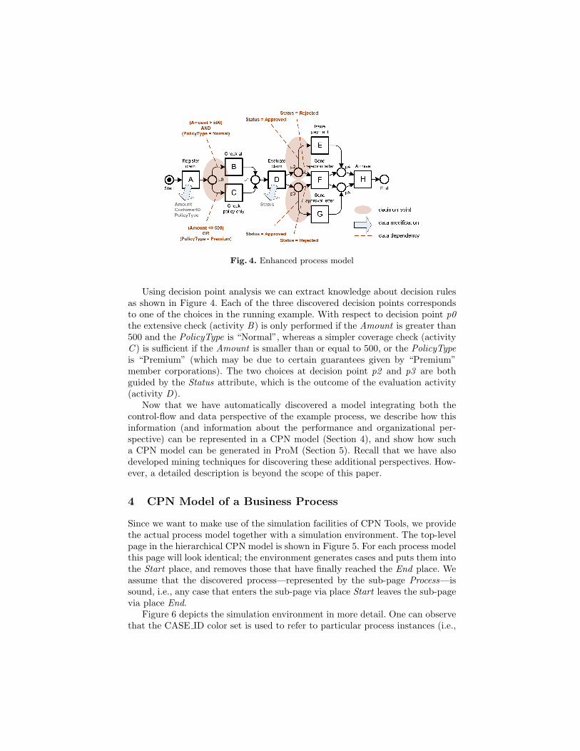
Fig. 4. Enhanced process model

Using decision point analysis we can extract knowledge about decision rulesas shown in Figure 4. Each of the three discovered decision points correspondsto one of the choices in the running example. With respect to decision point p0the extensive check (activity B) is only performed if the Amount is greater than500 and the PolicyType is “Normal”, whereas a simpler coverage check (activityC ) is sufficient if the Amount is smaller than or equal to 500, or the PolicyTypeis “Premium” (which may be due to certain guarantees given by “Premium”member corporations). The two choices at decision point p2 and p3 are bothguided by the Status attribute, which is the outcome of the evaluation activity(activity D).

Now that we have automatically discovered a model integrating both thecontrol-flow and data perspective of the example process, we describe how thisinformation (and information about the performance and organizational per-spective) can be represented in a CPN model (Section 4), and show how sucha CPN model can be generated in ProM (Section 5). Recall that we have alsodeveloped mining techniques for discovering these additional perspectives. How-ever, a detailed description is beyond the scope of this paper.

4 CPN Model of a Business Process

Since we want to make use of the simulation facilities of CPN Tools, we providethe actual process model together with a simulation environment. The top-levelpage in the hierarchical CPN model is shown in Figure 5. For each process modelthis page will look identical; the environment generates cases and puts them intothe Start place, and removes those that have finally reached the End place. Weassume that the discovered process—represented by the sub-page Process—issound, i.e., any case that enters the sub-page via place Start leaves the sub-pagevia place End.

Figure 6 depicts the simulation environment in more detail. One can observethat the CASE ID color set is used to refer to particular process instances (i.e.,

Environment

Environment

Process

Process

Start

CASE_ID

End

CASE_ID

Fig. 5. Overview page

cases). To give each case a unique ID a counter is simply incremented for eachgenerated process instance. For the data perspective, a separate token containingthe case ID and a record of case attributes (defined via the DATA color set) iscreated and initialized. The place Case data is modeled as a fusion place asactivities may need to inspect or modify data attribute values on different pagesin the hierarchical model. Furthermore, the Resources fusion place contains theavailable resources for the process, and therefore determines the environmentfrom an organizational perspective. Finally, each time a token is put back inthe next case ID place a time delay5 is added to it, which is used to steer thegeneration of new cases. In Figure 6 a constant time delay of 3 implements thatevery 3 time units a new case arrives. Note that the inter-arrival times may alsobe sampled from some probability distribution discovered by ProM.

(c,data)

(c, {Amount = 0,PolicyType = Normal,Status = Rejected})

c

cc+1 @+round(3.0)

c

Clean_upInit

Resources

Resources

["Howard","Fred","Mona","Vincent","Robert","Linda","John"]

RESOURCE

Case data

Case data CASE_IDxDATA

nextcase ID

1

CASE_ID

End

In CASE_ID

Start

Out CASE_IDOut In

Case data

Resources

Fig. 6. Environment page

Figure 7 shows the sub-page containing the actual process model, which looksexactly like the original, low-level Petri net. Note that the tokens routed fromthe Start to the End place are of type CASE ID, so that tokens belonging todifferent instances are not mixed up.5 Note that in our simulation model the time delay is always attached to an arc

(depending on the token that should be delayed) rather than using the time delayof a transition in order to avoid side effects on other tokens that should actually notbe delayed (such as the Case data token).

Sendrejection

letterSend rejection letter

Sendapproval

letterSend approval letter

Issuepayment

Issue payment

Evaluateclaim

Evaluate claim

Check policy only

Check policy only

Check all

Check all

Registerclaim

Register claim p5

p4

p3

p2

p1p0 End

Out

Start

InIn OutRegister claim

Check all

Check policy only

Evaluate claim

Issue payment

Send approval letter

Send rejection letter

Archiveclaim

Archive claimArchive claimCASE_IDCASE_ID

CASE_ID

CASE_ID CASE_ID

CASE_ID

CASE_IDCASE_ID

Fig. 7. Process page

Every activity on the process page has its own sub-page containing the actualsimulation information. Depending on the covered perspectives these activitysub-pages may look very different. In the following sub sections we will presenthow simulation information from several dimensions can be represented in termsof a CPN sub-page.

4.1 Data

Taking the enhanced model from Figure 4 as the starting point, we now wantto incorporate the discovered data dependencies in the simulation model. Thediscovered decision rules are based on attributes provided by activity Registerclaim and Evaluate claim respectively (see the result described in Section 3).Since the attribute CustomerID is not involved in the discovered rules, we discardit from the process model and define process-specific data types for each of theremaining attributes (i.e., AMOUNT, POLICYTYPE, and STATUS).

Fig. 8. Writing data items using random values

Figure 8 shows how the provision of case data can be modeled using randomvalues. While a random value for a nominal attribute can be generated by ap-plying the ran() function directly to the color set6 a dedicated random function6 Note that—for performance reasons—the ran() function can only be used for enu-

merated color sets with less than 100 elements.

is needed for numeric attributes. In the action part of transition Register claimcomplete function POLICYTYPE.ran() is used to select the policy type (“Nor-mal” or “Premium”) and a dedicated function randomAmount() is used to setthe amount. In this case, the amount is sampled from a uniform distributiongenerating a value between the lowest and the highest attribute value observedin the event log. However, many other settings are possible.

Fig. 9. Modeling data dependencies using transition guards

Figure 9 shows how the discovered data dependencies can then be modeledwith the help of transition guards. If the transition is enabled from a control-flowperspective, it additionally needs to satisfy the given guard condition in orderto be fired.

4.2 Time

Although there is no time information in the example event log, we want toinclude the time dimension in our simulation model because it is relatively easyto extract from most real-life logs. Moreover, this perspective is of utmost im-portance from a practical point of view. To explain this perspective we assumethat—in contrast to the policy-only check, which takes between 3 and 8 timeunits—the full check procedure needs between 9 and 17 time units to com-plete. Furthermore, the time between the point where the activity could havebeen started (i.e., all required previous activities were completed) and the pointwhere someone actually starts working on it may vary from 3 to 5 time units.Whereas the sub-page shown in Figure 9(a) models the activity Check all inan atomic way, one can distinguish between schedule, start, and complete transi-tions in order to incorporate the waiting time and execution time of this activity.Figure 10 shows three ways to model this for activity Check all.

Fig. 10. Different variants of modeling time on sub-page Check all depending on theevent types (i.e., schedule, start, and complete) present in the log

In Figure 10(a) only the execution time of the activity is modeled. Whentransition Check all start is fired, a token is produced with the indicated timedelay. Similar to the case generation scheme in Figure 6, the token will remainbetween 9 and 17 time units in place E (i.e., the activity is in the state Executing)before transition Check all complete may fire.

In Figure 10(b) both the execution time and the waiting time are explicitlymodeled. Analogously to the execution time, the waiting time is realized by atime delay that forces the token to reside in place W (i.e., the activity is in thestate Waiting) between 3 and 5 time units before transition Check all start mayfire.

In Figure 10(c) the sum of the waiting time and the execution time is mod-eled. This may be useful if no information is available about the actual start ofan activity (i.e., only the time when it becomes enabled and when it is finishedis known).

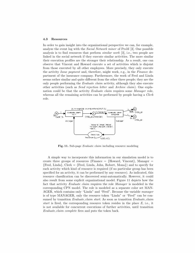
4.3 Resources

In order to gain insight into the organizational perspective we can, for example,analyze the event log with the Social Network miner of ProM [3]. One possibleanalysis is to find resources that perform similar work [3], i.e., two people arelinked in the social network if they execute similar activities. The more similartheir execution profiles are the stronger their relationship. As a result, one canobserve that Vincent and Howard execute a set of activities which is disjointfrom those executed by all other employees. More precisely, they only executethe activity Issue payment and, therefore, might work, e.g., in the Finance de-partment of the insurance company. Furthermore, the work of Fred and Lindaseems rather similar and quite different from the other three people; they are theonly people performing the Evaluate claim activity, although they also executeother activities (such as Send rejection letter and Archive claim). One expla-nation could be that the activity Evaluate claim requires some Manager role,whereas all the remaining activities can be performed by people having a Clerkrole.

Fig. 11. Sub-page Evaluate claim including resource modeling

A simple way to incorporate this information in our simulation model is tocreate three groups of resources (Finance = {Howard, Vincent}, Manager ={Fred, Linda}, Clerk = {Fred, Linda, John, Robert, Mona}) and to specify foreach activity which kind of resource is required (if no particular group has beenspecified for an activity, it can be performed by any resource). As indicated, thisresource classification can be discovered semi-automatically. However, it couldalso result from some explicit organizational model. Figure 11 depicts how thefact that activity Evaluate claim requires the role Manager is modeled in thecorresponding CPN model. The role is modeled as a separate color set MAN-AGER, which contains only “Linda” and “Fred”. Because the variable manageris of type MANAGER, only the resource token “Linda” or “Fred” can be con-sumed by transition Evaluate claim start. As soon as transition Evaluate claimstart is fired, the corresponding resource token resides in the place E, i.e., itis not available for concurrent executions of further activities, until transitionEvaluate claim complete fires and puts the token back.

4.4 Probabilities and Frequencies

Closely related to the modeling of time aspects is the likelihood of taking aspecific path. Both may be of a stochastic nature, i.e., a time duration may besampled from some probability distribution, and similarly, the selection of analternative branch may be selected randomly (if there are no data attributesclearly influencing the choice). Hence, the probabilistic selection of a path alsoneeds to be incorporated in the CPN model. Figure 12 shows how often eacharc in the model has been used, determined through the log replay analysiscarried out by the Conformance Checker in ProM7. Looking at the first choiceit becomes clear that activity Check policy only has been executed 7 (out of 10)times and activity Check all was performed only 3 times. Similarly, activity Sendrejection letter happened for 4 (out of 10) cases, while in 6 cases both activitySend approval letter and activity Issue payment were executed.

Fig. 12. Frequencies of alternative paths in the example model

In order to reflect frequencies of alternative paths in the simulation modelwe use two different approaches, depending on the nature of the choice.

Simple choice The first choice construct in the example model is consideredto be a so-called simple choice as it is only represented by one single place.We can model such a simple choice using a probability token that is sharedamong all the activities involved in this choice via a fusion place.Figure 13 shows this solution for the choice at place p0. Both sub-pages Checkall and Check policy only contain a fusion place p0 Probability that initiallycontains a token with the value 0, but after each firing of either transitionCheck all start or transition Check policy only start a random value between0 and 100 is generated. Because of the guard condition, the decision at theplace p0 is then determined for each case according to the current value ofthe token in place p0 Probability. For example, the transition Check all startneeds to bind the variable prob to a value greater than or equal to 70 inorder to be enabled, which will only happen in 30% of the cases.

7 Note that the place names and the markup of the choices have been added to thediagnostic picture obtained from ProM for explanation purposes.

Fig. 13. Using a probability token for simple choices

Dependent choices The second choice construct in the example model actu-ally consists of two dependent choices8 (i.e., the choices represented by placesp2 and p3 ) that need to be coordinated in order to either approve or rejecta claim. It is clear that two dependent choices cannot be steered properly bytwo independently generated probability tokens, because the process modelwill deadlock as soon as the values of the probability tokens indicate con-trasting decisions (e.g., the probability token in p2 indicates a reject whilethe other probability token in p3 suggests to approve the claim).Figure 14 shows a solution for modeling the dependent choices at place p2and p3. The idea is to increase the likelihood of choosing a certain activitythrough activity duplication (using the fact that during simulation in CPNTools all enabled transitions will be fired with an equal probability). Thisway, the observed relative frequency9 of the transitions involved in the de-pendent choices can be incorporated in the simulation model. Figure 14(a)shows an intermediate sub-page for activity Issue payment, where three sub-stitution transitions Issue payment point to different instances of the samesub-page Issue payment (i.e., the actual sub-page is only modeled once).Figures 14(b) and (c) show similar intermediate sub-pages for the activitiesSend approval letter (also duplicated three times) and Send rejection letter(duplicated twice).

8 Similar to the Decision Miner we consider each place as a choice (or decision point)if it contains more than one outgoing arc (cf. Figure 4).

9 In order to obtain the relative frequency, the absolute frequency is divided by thegreatest common divisor (i.e., 6/2 = 3 and 4/2 = 2).

Fig. 14. Modeling dependent choices via activity duplication

4.5 Logging and Monitoring Simulation Runs

The CPN models described in this section deal with time, resources, and data.When running a simulation in CPN Tools we are interested in statistics (e.g.average, variance, minimum, and maximum) related to (a) the utilization ofresources and (b) the throughput times of cases during the simulation run. Weobtain this information via pre-defined monitors as described in the following.

(a) Resource utilization. If resources have been specified for the process, allthe available resources are contained in a Resources fusion place, which is locatedon the Environment page and on every activity sub-page. For obtaining statisticsabout the resource utilization during the simulation we can define a marking sizemonitor [9] for this Resources fusion place, which records the number of availableresources plus the current time (and step) as soon as a resource becomes (un-)-available.

(b) Throughput time. If the time perspective is covered, tokens are createdwith a timestamp. We record the timestamp of each case’s creation togetherwith the case ID token that is routed through the process. This way, we candetermine the throughput time of a case by defining a data collector monitor[9] for the Clean up transition on the Environment page (cf. Figure 6), whichsimply calculates the difference between the current model time and the starttime of a case10, and records the throughput time, the end time and end step foreach case. Note that—due to recording its creation time—the current run timeof a case could be easily determined at any stage in the process via adding somecustom monitor.

10 Because the type of the current model time is infinite integer and in order to notlose precision when calculating the difference between the current model time andthe start time of a case, the model time is mapped onto a STRING value, i.e., colorset START TIME is of type STRING and is used to encode infinite integers.

Moreover, we want to generate process execution logs for the business processin the CPN model. This can be very useful for, e.g., the creation of artificial logsthat are needed to evaluate the performance of process mining algorithms.

For each firing of a transition on an activity sub-page an event is logged,which includes case ID, the type of transition (i.e., schedule, start, or complete),current timestamp, originator, and additional data (each if available). For gen-erating these process execution logs we use the logging functions that have beendescribed in [10]. However, in contrast to [10]—where the code segments of tran-sitions have to be modified to invoke these logging functions—we decided to useuser defined monitors [9] in order to clearly separate the logging from the restof the simulation model.

5 Exporting CPN Models from ProM

We are able to generate CPN models as presented in the previous section (i.e.,including simulation environment and the described monitors) using the CPNTools 2.0 Export plug-in in the ProM framework11. It either accepts a simula-tion model that has been provided by another plug-in in the framework, or asimple, low-level Petri net (in which case an empty simulation model is createdand filled with default values). Before the actual export takes place, it allowsfor the manipulation of the simulation information in the model. As illustratedin Figure 1, we have discovered a process model including the data perspective(provided by the Decision Miner), and we can now manually integrate infor-mation about further dimensions, such as the performance and organizationaldimension.

Figure 15(a) shows the global Configuration settings, where the user canchoose which dimensions should be included in the generated CPN model. In fact,although the relevant simulation information may be provided, it will be ignoredif the corresponding configuration option was not chosen. Note that, since thewaiting time of an activity typically results from the unavailability of resources,the explicit modeling of a resource scheme such as in Figure 11 is in conflict withmodeling the time dimension including waiting time (cf. figures 10(b) and (c)).Therefore, only the execution time option is available if the resource dimensionis selected.

Figure 15(b) depicts the Attribute settings of the process. New data attributescan be provided by specifying their name, type (nominal or numeric), possiblevalues (a list of String values for a nominal attribute, and some probabilitydistribution12 for a numeric one), and initial value. Note that for our exampleprocess the available data attributes were already discovered by the Decision

11 Note that the layout of the generated models was slightly adjusted in order to im-prove the readability.

12 The CPN Export plug-in supports all probability distributions currently availablein CPN Tools, i.e., constant, bernoulli, binomial, chi square, discrete, erlang, expo-nential, normal, poisson, student, and uniform.

Fig. 15. CPN Tools export settings

Miner. For this particular example it makes sense to delete the CustomerIDattribute, since it is not involved in any of the discovered data dependencies.

In Figure 15(c), a screenshot of the Activity settings for activity Registerclaim is displayed. In this view, the provided data attributes, the executiontime, waiting time, sojourn time, and the required resource group may be spec-ified for each of the activities in the process. The data attributes were alreadyprovided by the Decision Miner, and we can decide whether the old value of theattribute should be kept (i.e., reuse) or whether a random value will be gener-ated (i.e., re-sample). Furthermore, we can assign some execution time (note theuniform distribution between 2 and 4 time units), and choose the suitable groupof resources from the list of groups available in the process (note the Clerk role).

Figure 15(d) shows the Choice configuration view, where the user can deter-mine for each decision point in the process whether it should be based on either

probabilities or frequencies (cf. Section 4.4), or on data attributes, or whetherit should not be guided by the simulation model (one of the alternative paths isthen randomly chosen by CPN Tools). In Figure 15(d) the probability settingsare displayed. For every alternative branch a probability may be provided be-tween 0.0 and 1.0. Before the actual export takes place, each value is normalizedby the sum of all specified values, and if the values sum up to 0.0, default values(i.e., equal probabilities for each alternative branch) are used. As discussed inSection 4.4, for dependent choices one should specify a relative frequency valueinstead. Finally, we can provide a dependency value based on data attributes(in the case of our example process the discovered dependency has already beenfilled in by the Decision Miner). In the current version of the export plug-in thisdependency value is simply a String containing the condition to be placed in thetransition guard of the corresponding transition.

In Figure 15(e) the Resource settings are depicted. Here, one can add groupsand resources, and assign resources to groups. This way, the CPN Export plug-inalso supports the specification of information about resources. This informationis then used to create the sub-pages shown earlier.

6 Related Work

The work reported in this paper is related to earlier work on process mining,i.e., discovering a process model based on some event log. The idea of applyingprocess mining in the context of workflow management was first introduced in[7]. Cook and Wolf have investigated similar issues in the context of software en-gineering processes using different approaches [8]. Herbst and Karagiannis alsoaddress the issue of process mining in the context of workflow management usingan inductive approach [12]. They use stochastic task graphs as an intermediaterepresentation and generate a workflow model described in the ADONIS mod-eling language. Then there are several variants of the α algorithm [6, 20]. In [6]it is shown that this algorithm can be proven to be correct for a large class ofprocesses. In [20] a heuristic approach using rather simple metrics is used toconstruct so-called “dependency/frequency tables” and “dependency/frequencygraphs”. This is used as input for the α algorithm. As a result it is possible totackle the problem of noise. For more information on process mining we referto a special issue of Computers in Industry on process mining [5] and a surveypaper [4]. However, as far as we know, this is the first attempt to mine processmodels including other dimensions, such as data. (Note that [3] only considersthe social network in isolation and does not use it to provide an integrated view.)

In [11] the authors present a translation of Protos simulation models to CPNTools. In addition, three types of data collector monitors (measuring the to-tal flow time per case, the waiting time per task, and the resource availabil-ity/utilization per resource type), and configuration features enabling the dy-namic elimination of unnecessary parts of the process model are generated. Be-sides the work in [11], we are not aware of further attempts to export businessprocess models to CPN Tools. The work reported in this paper has a different

starting point as it is not limited by the simulation information present in a Pro-tos model, but aims at discovering the process characteristics to be simulatedfrom the event logs of real process executions.

7 Future Work

Future work includes the refinement of the generated CPN models. For example,a more realistic resource modeling scheme may allow for the specification of aworking scheme per resource (e.g., whether the person works half-time or full-time) and include different allocation mechanisms. Moreover, we plan to applyour approach to real-life data. Finally, the discovery of further perspectives ofa business process will be integrated in the mined process models. Currently,we are able to discover data dependencies via the Decision Miner in ProM. Butexisting plug-ins in ProM deliver also time-related characteristics of a process(such as the case arrival scheme, and execution and waiting times) and frequen-cies of alternative paths, or organizational characteristics (such as the roles ofthe employees involved in the process). All these different pieces of aggregateinformation (discovered from the event log) need then to be combined in oneholistic simulation model, which may be exported to CPN Tools, or, e.g., trans-lated to an executable YAWL model [2]. Note that a YAWL model can be usedto enact a business process using the YAWL workflow engine. For enactment allperspectives play a role and need to be taken into account. Hence, successfullyexporting to YAWL is another interesting test case for the mining of processmodels with data and resource information.

Acknowledgements

This research is supported by EIT and the IOP program of the Dutch Ministry ofEconomic Affairs. Furthermore, the authors would like to thank Ton Weijters,Boudewijn van Dongen, Ana Karla Alves de Medeiros, Minseok Song, LauraMaruster, Christian Gunther, Eric Verbeek, Monique Jansen-Vullers, Hajo Rei-jers, Michael Rosemann, Huub de Beer, Peter van den Brand, et al. for theiron-going work on process mining techniques. We would also like to thank LisaWells and Kurt Jensen for their support in using CPN Tools.

References

1. W.M.P. van der Aalst. Business Alignment: Using Process Mining as a Tool forDelta Analysis. In J. Grundspenkis and M. Kirikova, editors, Proceedings of the 5thWorkshop on Business Process Modeling, Development and Support (BPMDS’04),volume 2 of Caise’04 Workshops, pages 138–145. Riga Technical University, 2004.

2. W.M.P. van der Aalst and A.H.M. ter Hofstede. YAWL: Yet Another WorkflowLanguage. Information Systems, 30(4):245–275, 2005.

3. W.M.P. van der Aalst, H.A. Reijers, and M. Song. Discovering Social Networksfrom Event Logs. Computer Supported Cooperative Work, 14(6):549–593, 2005.

4. W.M.P. van der Aalst, B.F. van Dongen, J. Herbst, L. Maruster, G. Schimm, andA.J.M.M. Weijters. Workflow Mining: A Survey of Issues and Approaches. Dataand Knowledge Engineering, 47(2):237–267, 2003.

5. W.M.P. van der Aalst and A.J.M.M. Weijters, editors. Process Mining, SpecialIssue of Computers in Industry, Volume 53, Number 3. Elsevier Science Publishers,Amsterdam, 2004.

6. W.M.P. van der Aalst, A.J.M.M. Weijters, and L. Maruster. Workflow Mining:Discovering Process Models from Event Logs. IEEE Transactions on Knowledgeand Data Engineering, 16(9):1128–1142, 2004.

7. R. Agrawal, D. Gunopulos, and F. Leymann. Mining Process Models from Work-flow Logs. In Sixth International Conference on Extending Database Technology,pages 469–483, 1998.

8. J.E. Cook and A.L. Wolf. Discovering Models of Software Processes from Event-Based Data. ACM Transactions on Software Engineering and Methodology,7(3):215–249, 1998.

9. CPN Group, Aarhus. CPN Tools Help. http://wiki.daimi.au.dk/cpntools-help/.10. A.K. Alves de Medeiros and C.W. Guenther. Process Mining: Using CPN Tools

to Create Test Logs for Mining Algorithms. In K. Jensen, editor, Proceedings ofthe Sixth Workshop and Tutorial on Practical Use of Coloured Petri Nets and theCPN Tools, pages 177–190, 2005.

11. F. Gottschalk, W.M.P. van der Aalst, M.H. Jansen-Vullers, and H.M.W. Verbeek.Protos2CPN: Using Colored Petri Nets for Configuring and Testing Business Pro-cesses. Accepted for the Seventh Workshop and Tutorial on Practical Use ofColoured Petri Nets and the CPN Tools, 2006.

12. J. Herbst. A Machine Learning Approach to Workflow Management. In Proceedings11th European Conference on Machine Learning, volume 1810 of Lecture Notes inComputer Science, pages 183–194. Springer-Verlag, Berlin, 2000.

13. K. Jensen. Coloured Petri Nets. Basic Concepts, Analysis Methods and PracticalUse. Springer-Verlag, 1997.

14. T. M. Mitchell. Machine Learning. McGraw-Hill, 1997.15. J. R. Quinlan. C4.5: Programs for Machine Learning. Morgan Kaufmann, 1993.16. A. Rozinat and W.M.P. van der Aalst. Conformance Testing: Measuring the Fit

and Appropriateness of Event Logs and Process Models. In C. Bussler et al., editor,Business Process Management 2005 Workshops, volume 3812 of Lecture Notes inComputer Science, pages 163–176. Springer-Verlag, Berlin, 2006.

17. A. Rozinat and W.M.P. van der Aalst. Decision Mining in Business Processes.BPM Center Report BPM-06-10, BPMcenter.org, 2006.

18. A. Rozinat and W.M.P. van der Aalst. Decision Mining in ProM. In S. Dustdar,J.L. Fiadeiro, and A. Sheth, editors, BPM 2006, volume 4102 of Lecture Notes inComputer Science, pages 420–425. Springer-Verlag, Berlin, 2006.

19. A. Vinter Ratzer, L. Wells, H. M. Lassen, M. Laursen, J. F. Qvortrup, M. S.Stissing, M. Westergaard, S. Christensen, and K. Jensen. CPN Tools for Editing,Simulating, and Analysing Coloured Petri Nets. In W.M.P. van der Aalst andE. Best, editors, Applications and Theory of Petri Nets 2003: 24th InternationalConference, ICATPN 2003, volume 2679 of Lecture Notes in Computer Science,pages 450–462. Springer Verlag, 2003.

20. A.J.M.M. Weijters and W.M.P. van der Aalst. Rediscovering Workflow Modelsfrom Event-Based Data using Little Thumb. Integrated Computer-Aided Engi-neering, 10(2):151–162, 2003.

21. I. H. Witten and E. Frank. Data Mining: Practical Machine Learning Tools andTechniques, 2nd Edition. Morgan Kaufmann, 2005.

Business Process Simulation - A Tool Survey

M.H. Jansen-Vullers and M. Netjes

Department of Technology Management, Eindhoven University of TechnologyP.O. Box 513, NL-5600 MB, Eindhoven, The Netherlands.

{m.h.jansen-vullers, m.netjes}@tm.tue.nl

Abstract. In the nineties, more and more attention was raised for pro-cess oriented analysis of the performance of companies. Nowadays, manyprocess aware information systems are implemented (e.g., workflow man-agement systems) and business processes are evaluated and redesigned.The discipline related to this field of study is called Business ProcessManagement (BPM). An important part of the evaluation of designedand redesigned business processes is Business Process Simulation (BPS).Although an abundance of simulation tools exist, the applicability ofthese tools is diverse. In this paper we discuss a number of simulationtools that are relevant for the BPM field, we evaluate their applicabilityfor BPS and formulate recommendations for further research.

Keywords: Business Process Management, Simulation, Petri nets.

1 Introduction

Business Process Management (BPM) is attracting attention more than a decadenow, and its attention is now shifting from the enactment of business processestowards improving business processes. The field of BPM now supports the de-sign, enactment, control, and analysis of business processes [6]. Companies areimproving their performance by a constant evaluation of the value added in allparts of their processes. Business processes are in a continuous improvementcycle in which design and redesign play an important role. Various possibilitiesto change a process are present and the best alternative design should replacethe current process. Making an intuitive choice may lead to unpleasant surprisesand lower process performance instead of yielding the expected gains. In [16]simulation is mentioned as one of the techniques suitable for the support of re-design. The simulation of business processes helps in understanding, analyzing,and designing processes. With the use of simulation the (re)designed processescan be evaluated and compared. Simulation provides quantitative estimates ofthe impact that a process design is likely to have on process performance and aquantitatively supported choice for the best design can be made.

Simulating business processes is, to a large extent, overlapping with the sim-ulation of other discrete event systems. In [32] an overview is provided of thesteps that are carried out in the context of Business Process Simulation (BPS).

Regarding the simulation of business processes a number of steps can be distin-guished.

First the business process is mapped onto a process model, possibly sup-plemented with process documentation facilities. Then the sub processes andactivities are identified. The control flow definition is created by identifying theentities that flow through the system and describing the connectors that link thedifferent parts of the process. Lastly, the resources are identified and assigned tothe activities where they are necessary. The process model should be verified toensure that the model does not contain errors.

Before simulation of a business process, the performance characteristics, suchas throughput time and resource utilization, need to be included. For statisti-cally valid simulation results a simulation run should consists of multiple subruns and each of these sub runs should have a sufficient run length. During thesimulation, the simulation clock advances. The simulation tool may show ananimated picture of the process flow or real-time fluctuations in the key perfor-mance measures. When the simulation has been finished, the simulation resultscan be analyzed. To draw useful and correct conclusions from these results, sta-tistical input and output data analysis is performed.

Although the steps in BPS will be the same irrespective of the simulation toolused, each simulation tool will have a different applicability. There is an abun-dance of simulation tools available of which some are applicable to the BPMfield. In this paper we discuss several simulation tools taken from three relevantareas: business process modelling, business process management and generalsimulation tools. We evaluate the modelling, simulation and output analysis ca-pabilities and we aim at providing insights in the advantages and disadvantagesof each simulation tool.

The remainder of this paper is organized as follows. First, we discuss relatedwork on evaluation criteria of BPM tools. Then, in Section 3, we describe toolsfor BPS. The criteria used for the evaluation of BPS tools are listed and explainedin Section 4. In Section 5 we compare the described BPS tools, and in Section 6we present our conclusions.

2 Related work

In this paper, we aim to evaluate several software packages for suitability of BPS.Hardly any package explicitly advertises as BPS tool, however, many of themprovide simulation functionality and may be suitable. Bradley et al defined sevendifferent categories to evaluate business process re-engineering software tools [8].The seven categories are as follows:

1. Tool capabilities, including a rough indication of modelling, simulation andanalysis capabilities.

2. Tool hardware and software, including, e.g., the type of platform, languages,external links and system performance.

3. Tool documentation, covering the availability of several guides, online-helpand information about the learning curve of the tool.

4. User features: amongst others user friendliness, level of expertise required,and existence of a graphical user interface.

5. Modelling capabilities, such as identification of different roles, model in-tegrity analysis, model flexibility and level of detail.

6. Simulation capabilities, summarizing the nature of simulation (discrete vs.continuous), handling of time and cost aspects and statistical distributions.

7. Output analysis capabilities such as output analysis and BPR expertise.

In this paper we elaborate on the categories as defined by Bradley et al inthe direction of BPS. Especially the last three categories are of interest whenevaluating BPS.

With respect to modelling capabilities, the patterns research is used to eval-uate the possibility to model various control flow patterns [5], data patterns[26] and resource patterns [27]. The patterns research is used to evaluate themodelling capabilities of a tool with respect to complexity.

The complexity of modern business processes is increasing. In order to man-age this complexity, Becker et al have formulated six main quality criteria forbusiness process models [7]. These criteria are:

1. Correctness, the model needs to be syntactically and semantically correct.2. Relevance, the model should not contain irrelevant details.3. Economic efficiency, the model should serve a particular purpose that out-

weighs the cost of modelling.4. Clarity, the model should be (intuitively) understandable by the reader.5. Comparability, the models should be based on the same modelling conven-

tions within and between models.6. Systematic design, the model should have well-defined interfaces to other

types of models such as organizational charts and data models.

Many authors have proposed requirements for business process modellingtools (for example [10, 24, 31, 35]) or have tested these requirements empirically[11, 16]. Although this requirement building frequently took place in the contextof BPS only one explicit list with evaluation criteria for simulation or outputanalysis capabilities is present. Law and Kelton describe desirable software fea-tures for the selection of general purpose simulation software [19]. They identifythe following groups of features:

1. General capabilities, including modelling flexibility and ease of use.2. Hardware and software considerations.3. Animation, including default animation, library of standard icons, control-

lable speed of animation, and zoom in and out.4. Statistical capabilities, including random number generator, probability dis-

tributions, independent runs (or replications), determination of warm upperiod, and specification of performance measures.

5. Customer support and documentation.6. Output reports and plots, including standard reports for the estimated per-

formance measures, customization of reports, presentation of average, min-imum and maximum values and standard deviation, storage and export ofthe results, and a variety of (static) graphics like histograms, time plots, andpie charts.

3 Tools for Business Process Simulation

Many software tools exist to simulate processes. When simulating business pro-cesses, some specific requirements are applicable. The nature of the businessprocess requires sufficient modelling power of the tool. When particular choicesor a synchronization cannot be implemented, the simulation result loosens itsstrengths. On the other hand, simulation of business processes aims to supportprocess owners or process managers. When the tool or the simulation output canhardly be understood by the client, the tool overreaches itself. In this section,we describe three different categories of software tools that may be applicablefor BPS:

– business process modelling tools,– business process management tools,– general purpose simulation tools.

For each type a general introduction and the description of two specific toolsare given.

3.1 Business process modelling tools

Business Process Modelling tools are developed to describe and analyze busi-ness processes. The analysis part may provide data useful for the managementof these processes. The tool supports the process to establish the control flowof business processes, the resource roles involved, documents being used and itdocuments instructions for the execution of steps in the business process. As a re-sult, reports can be generated for process documentation, manuals, instructions,functional specifications, etc. For the evaluation of the simulation functionalitywe consider two different tools, one based on Petri Nets (Protos) and one basedon Event-driven Process Chains (ARIS Toolset).

ProtosProtos is a modelling and analysis tool developed by Pallas Athena and it ismainly applied for the specification of in-house business processes. Protos issuitable to model well-defined Petri Net structures. Nevertheless, it also permitsfree hand specifications of business processes without formal semantics, e.g. tosupport initial and conceptual modelling [34]. When formal Petri Net semanticshave been applied, translation to various other process-based systems is feasi-ble as well, e.g. to the workflow management system COSA and the workflowanalyzer Woflan [33].

The main use of Protos is to define models of business processes as a steptowards either the implementation of quality management systems, the redesignof a business process, communication enhancement between process stake holdersor the implementation of workflow management systems. The process can beanalyzed with respect to data, user and control logic perspective, and by makinguse of simulation [34].

The simulation engine is implemented in Protos version 7.0. The existingengine of the Petri Net based tool ExSpect has been integrated in the Pro-tos environment and it facilitates the simulation of the business process as hasbeen specified in the Protos model before. In addition to the standard processspecification, simulation data can be added for tasks, connections and resourcessuch as the (stochastic) processing time and the number of resources required.Furthermore, process characteristics are added such as the arrival pattern forcases and the number and length of simulation runs. The simulation result canbe obtained from an Excel spreadsheet and includes mean and 90% and 99%confidence interval of utilization rates, waiting times, service times, throughputtimes and costs.

ARISARIS Simulation is a professional tool for the dynamic analysis of business pro-cesses. It is an integral part of the ARIS Toolset; processes recorded in the ARISToolset are used as the data basis for business process simulation. ARIS Toolsetis developed by IDS Scheer AG (see www.ids-scheer.nl) and can be classifiedas an enterprise modelling tool with a strong emphasis on business processes.Enterprise modelling is supported by a number of different views (process, func-tion, data, organization and product) and the modelling approach called ARISHouse [30, 29].

The process modelling part supports the definition of business processes rep-resented in Event-driven Process Chains (EPCs). Other modelling techniquessupported in the ARIS House are, e.g. value chains (also to model the controlflow), organization charts (to model relationships between resources), EPCs andand function allocation diagrams (for supplementary information such as dataand systems). The simulation functionality shows whether the specified pro-cesses are executable at all and it answers questions about throughput timesand utilization levels of the resources, etc.

When starting a simulation, the simulation module of the tool is startedand the model is transferred. The simulation toolbar shows buttons for startand stop, one time step and simulation steps and options for animations. Thesimulation results are available in Excel spreadsheets and include statistics onevents, functions, resources, processes and costs. Only raw data is available.

3.2 Business process management tools

Business process management (BPM) systems can be seen as successors of Work-flow Management (WFM) systems. The core functionality of a WFM system isautomating the “flow of work”. With the introduction of BPM the functionality

is broadened to support the whole proces life-cycle. BPM is defined as Support-ing business processes using methods, techniques, and software to design, enact,control, and analyze operational processes involving humans, organizations, ap-plications, documents and other sources of information [6]. Some BPM toolsoffer a simulation tool to support the design phase. Most BPM tools, however,do not provide simulation facilities and we use FLOWer as a representative ofthis group of BPM tools. Further, we will evaluate FileNet, one of the mostadvanced BPM tools. FileNet is evaluated to show what most likely will be thebest simulation functionality provided by a BPM tool. The FLOWer tool isevaluated, regardless his lack of simulation facilities, to illustrate the other endof the simulation spectrum of BPM tools.

FLOWerFLOWer is a flexible, case-based BPM system. When handling cases the systemonly prevents actions for which it is specified that these are not allowed. Thisresults in a flexible process where activities for a case can be executed, skippedor redone.

The FLOWer systems consists of a FLOWer Studio, FLOWer Case Guide,FLOWer CFM (Configuration Management), FLOWer Integration Facility, andFLOWer Management Information and Case History Logging.

The graphical design environment, Studio, is used to define processes, activi-ties, precedences, data objects and forms. Work queues are used to provide workto users (defined with CFM) and to find cases satisfying specified search crite-ria. Case Guide is the client application which is used to handle individual cases.FLOWer Integration Facility provides the functionality to interface with otherapplications. FLOWer Management Information and Case History Logging canbe used to store and retrieve management information at various levels of detail.

BPM systems, like FLOWer, focus on the configuration of the system, andthe execution and control of the workflow. Additional features like the FLOWerManagement Information and the FLOWer Integration Facility are provided.However, FLOWer does not provide explicit simulation or output analysis func-tionality. We will not be able to evaluate the simulation and output analysiscapabilities of FLOWer, but we can evaluate the modelling capabilities [3, 5].

FileNetFileNet is considered to be one of the leading commercial BPM systems1. Wehave evaluated the strengths and weaknesses of the FileNet P8 BPM Suite andits ability to support the various parts of the process life-cycle [23].

The FileNet system includes a FileNet Process Designer, a FileNet ProcessSimulator, a FileNet Process Engine, a FileNet Process Administrator, and aFileNet Analysis Engine.

First, a process structure is modelled graphically with the Process Designerand tasks are assigned to work queues. These work queues and the associatedusers are created outside the Process Designer. Then, the created process defini-

1 www.gartner.com

tion is feeded to the Process Engine to start the execution of the workflow. Theexecution data for individual cases is logged by the Process Engine and can beaccessed with the Process Administrator. Further, execution data is aggregatedand parsed to the Analysis Engine. Reporting and analysis of the aggregateddata is facilitated by twenty out-of-the-box reports; each graphically presentingthe data related to one performance indicator.

The Process Simulator in FileNet can be used to evaluate the performanceof a created design. The Process Simulator is a separate tool, which can partlyimport the created process definition. Other parts of the process definition haveto be reentered. Simple arrival patterns of cases are defined, i.e. a fixed numberof cases arrives at fixed time points. Also historic, execution arrival data canbe used. Other performance characteristics should be added manually and canonly have constant values. After simulation an animation and a summary ofthe simulation results are provided. Simulation data can also be presented inExcel reports. However, performing what-if analysis (comparing scenarios) isnot possible.

3.3 General purpose simulation tools

Simulation tools may be tailored towards a specific domain, such as logistics(e.g., Enterprise Dynamics) or SPEEDES in the military domain. In this sectionwe consider simulation tools that are not tailored towards a particular domainand we evaluate their suitability for the domain of business processes. The firsttool, Arena, has an industrial background and shows industry successes in manu-facturing, supply chain management, military/defense, health care, contact cen-ters and process reengineering (see www.arenasimulation.com). The second tool,CPN Tools, has been developed in a university environment and has been appliedin more technical engineering domains (see http://www.daimi.au.dk/CPnets/).

ArenaArena is a general purpose simulation tool developed by Rockwell Automation.The Arena product family consists of a Basic Edition for uncomplicated pro-cesses and a Professional Edition for more complex large scale projects in man-ufacturing, distribution, processes, logistics, etc. The Professional Edition alsoprovides (and allows definition of) templates for complex repetitive logic, e.g.,for packaging and contact centers.

When opening the tool, a number of process panels are available, e.g., forbasic and advanced processes and for reporting. The model can be created bydrag and drop from the process panel to the model window. By double-clickingon the icons, options for the different building blocks can be set such as delaytypes, time units and the possibility to report statistics. Many more buildingblocks are available and can be attached when necessary.

When a model has been created and is completely specified (from the Arenaviewpoint) and it is syntactically correct, it can be simulated. Warm-up and cool-down periods can be specified, as well as run length and confidence intervals.

Several statistics are provided by default, but the larger part needs to be addedmanually by adding record building blocks where necessary [15].

In a previous study, de Vreede et al considered the suitability of Arena tosimulate business processes [35]. They stated that a weak point in simulatingbusiness processes is the time consuming and complicated process to create sim-ulation models. They took advantage of the possibility to develop their owntemplate with predefined building blocks, which they considered to be success-ful in several simulation studies they carried out.

CPN ToolsCPN Tools is developed by the computing science group of Aarhus Universityin Denmark. CPN Tools is a tool for editing, simulating and analyzing Col-ored Petri Nets. The tool attracts attention with respect to its user interfacewhich has been designed in cooperation with leading HCI experts, and includesa number of novel interaction mechanisms such as the use of two-handed inputby means of a mouse and a trackball. During editing a net (a process model),feedback facilities provide contextual error messages and indicate dependencyrelationships between net elements. The tool features incremental syntax check-ing and code generation which take place while a net is being constructed. Afast simulator efficiently handles both untimed and timed nets. Untimed netsare generally not applicable for modelling and simulation of (realistic) businessprocesses, but several earlier projects already showed that timed CP-nets canmodel business processes [20, 13, 22]. Correctness of the developed model canbe researched by existing Petri Net techniques such as the generation of statespaces and the analysis of boundedness and liveness properties, which are allimplemented in CPN Tools.

The industrial use of CPN Tools (and its predecessor Design CPN) can befound starting from the home page (http://www.daimi.au.dk/CPnets/). DesignCPN is the most widespread software package for modelling and analysis bymeans of Colored Petri Nets. The overview shows a wide variety of mainly tech-nical domain areas such as protocols and networks, hardware and control sys-tems. Also some projects are listed with a more business oriented focus, thoughthese are exceptions.

4 Evaluation criteria for BPS Tools

When evaluating BPS tools, the modelling, simulation and output analysis ca-pabilities of the tool are important. In this section we present our view on thesecapabilities and specify criteria to evaluate each capability in detail.

4.1 Modelling capabilities

The purpose of the modelling capabilities criteria is to evaluate how well andhow precise a business process can be represented. The modelling evaluationcriteria are:

– Ease of model building [8, 19]Model building should be easy to allow users to be involved in the modellingof their processes. A graphical user interface with predefined business ob-jects which can be dragged and dropped facilitates the model building. Thehard coding of process parts is hard to perform or understand for users andshould be avoided.

– Formal semantics [4] and verification of correctness [21, 33]Formal semantics provide a precise and unambiguous description of the be-havior of the modelled process. Van der Aalst concludes that many mod-elling techniques lack formal semantics and thus powerful analysis methodsand tools [4]. In [2] he summarizes three good reasons for using a Petri-net based workflow management system which appear to be critical in largeBPM projects. These reasons are: (1) the existence of formal semantics de-spite the graphical nature, (2) the state based diagrams instead of eventbased diagrams (as can be encountered in many workflow products) and (3)the abundance of analysis techniques.

– Workflow patterns [5]The workflow patterns [5], or control flow patterns, are used to evaluate theexpressive power of modelling languages. The patterns identify both basicand complex modelling constructs. The number of supported patterns indi-cate how well a modelling language can give a good representation of theactual business process.

– Resource and data perspective [8, 26, 27]The process model should include the resource and data perspective and notjust the process structure to provide a good representation of the real worldsituation. Resource and data patterns capture the various ways in which re-spectively resources and data are represented and utilized in processes [26,27].

– Level of detail, transparency and suitability for communication [7, 8]Both senior management as well as end users need to be informed about theprocess (alternatives), they shoulddddd be able to validate the model andshould be able to make decisions based on these models. These stake holdershave a different need for information, senior management wants a high leveloverview, while the end users need detailed work descriptions. Through theuse of, for instance, hierarchical layers processes are be modelled in detail,but without loosing overview.

4.2 Simulation capabilities

The purpose of the simulation capabilities is to evaluate in which way a sim-ulation can be carried out and which parameter settings can be made. Thesimulation evaluation criteria are:

– Performance dimensions [8, 25, 19]A simulation model should incorporate the performance dimensions one isinterested in. In most cases it should be possible to simulate several differ-ent time and/or costs aspects. Other relevant performance dimensions arequality and flexibility [25].

– Distributions [19, 24]The average performance of a simulated process may seem fine while in reallife many problems would occur because of its variability. Queues may beempty at some moments and overloaded at other moments, creating em-ployee and customer dissatisfaction [24]. Taking into account the distribu-tions of performance characteristics will not only show the average behaviorof the process, but also its extremities.

– Animation [19, 35]With simulation not only the final simulation results but also the simulationitself can give useful insights in the simulated process. A replay or anima-tion of the simulation will show the states the simulation model has beenin during simulation. This visualization might reveal bottlenecks and otherproblems in the execution of the process.

– Scenarios [14, 18]With the use of scenarios the consequences of changes can be investigated.While the process stays the same, different configurations of the simulationmodel reflect potential changes in, i.e., the arrival pattern or resource avail-ability. With the use of scenarios the effects of changes can be predicted andcounter measures can be taken to avoid bad performance once the changeoccurs in reality.

4.3 Output analysis capabilities

The output analysis capabilities aim to evaluate the outcome of a simulation,which data can be analyzed and which representation styles are provided. Theoutput analysis evaluation criteria are:

– Statistics [17, 19]Simulation should provide statistically proper results and it should be clearhow these results are calculated. Simulation settings (e.g. simulation length,number of replications, start and stop conditions [9, 24]) should be indicatedto or even better be set by the user. A random generator should be used forthe generation of cases. For each performance measure not only the mean,but also the standard deviation and confidence intervals should be presented.

– Format [8, 19]The tool should have an easy to read format for the presentation of the re-

sults and possibilities for animation, storing and reuse of results.

– What-if analysis [18, 9, 14]Before a process design is chosen what-if analysis is performed. In this anal-ysis different scenarios (of the same simulation model) are compared. Thecomparison of confidence intervals of a performance measure shows whichscenarios perform significantly better than others on this measure. It also in-dicates under which conditions a certain process design will perform withinits requirements and under which conditions a performance level can not bereached.

– Conclusion-making support [8, 35]Conclusion-making support facilitates the interpretation of the simulationresults. Useful support is the identification of trends, the slicing and dicingof data and the tracking of the cause of specific outcomes.

5 Comparison of BPS Tools

In Section 3 we described six different tools which may be applicable for BPS, andwhich have been developed from various viewpoints: process modelling, processexecution and simulation. In Section 4 we developed a framework with a set ofevaluation criteria to find strengths and weaknesses of these tools. In this section,we report our findings. We will score the BPS tools for each of the evaluationcriteria ranging from good (++) and neutral (+/–) to bad (– –).

5.1 Modelling capabilities

In this section we evaluate how well and how precise a business process can bemodelled in the tools. We provide a short overview per tool and at the end ofthe section we summarize the findings in Table 1.

ProtosThe control flow of a business process and the resources can very easily be spec-ified in Protos, as may be expected from a process modelling tool. Also the dataperspective and instructions for the execution of tasks can be specified. Thetool allows freehand specifications, however it also allows well-defined Petri Netstructures, thus opening possibilities for further verification (e.g., in Woflan) andanalysis (based on the ExSpect tool). The application of sub models allows fora transparent process model and handling of resources which can very well becommunicated with process owners. Points for improvement are the possibilityto assign different roles to one task and to specify part time work and overtime.This could be specified, e.g., in histograms (which can already be handled bythe simulation engine but is not (yet) allowed in the Protos interface).

ARISThe control flow part is being modelled in EPCs. This is an informal mod-elling language, and the simulation relies on the given semantics when the EPClanguage has been implemented in the ARIS Toolset. It appears that these se-mantics are not completely clear, which may result in unforseen behavior whenusing (X)OR connectors. The models can be conveniently arranged, has func-tional use of colors for different model elements and supports hierarchy. Dueto the informal language, several workflow patterns cannot be modelled conve-niently. Model verification is not supported by the tool.

FLOWerWith FLOWer it is, on the one hand, possible to handle exceptions and on theother hand, to force a sequential order handling. Due to this flexibility FLOWersupports most of the workflow patterns. FLOWer is data driven, giving it astrong data perspective and also the resource perspective is taken into account.Both the process and role graph can be modelled in several layers of detail.

FileNetMost BPM tools, including FileNet, use a simple graphical representation of pro-cess models without formal semantics and verification of correctness. With this,users can create and discuss process models without difficulties. More advancedworkflow patterns and also the resource and the data perspective need to behard coded in FileNet.

ArenaArena models can be created very easily, though to specify exactly those thingsyou would like to model is more difficult. When browsing through a model, thelevel of detail is very convenient, due to the use of sub models and the fact thatmany details are hidden in the icon properties. When creating models, goodknowledge about all necessary building blocks and their exact specification isrequired. Frequently used control flow patterns are supported, but some moreadvanced patterns require a bit more indirect modelling [12].

CPN ToolsThe tool is based on Petri Net modelling techniques, and both benefits andsuffers from this property: it has formal semantics, allows for most control flowpatterns [5] and can be verified, but the price to be paid is that the models maybe quite detailed and technical.

This level of detail is required to model resource handling and correspondingtiming aspects, which is crucial in most business process models. Also, some con-structs can only be modelled indirectly, thus resulting in model parts that canhardly be understood by business process owners. As a result, models cannot bebuilt easily. Though very powerful, the Petri Net formalism appears to be moredifficult to understand than informal modelling languages [28].

In Table 1 our score for the modelling capability criteria for each of the toolsis presented.

Table 1. Modelling capabilities

Feature Protos ARIS FLOWer FileNet Arena CPN Tools

Ease of model building ++ + + + + – –Formal semantics/verif. + – – – – – +/– ++Workflow patterns + – + +/– + +Resources and data + ++ ++ +/– + +/–Level of detail ++ ++ ++ + ++ – –

5.2 Simulation capabilities

In this section, we evaluate in which way a simulation can be carried out andwhich parameter settings can be made. We provide a short overview per tooland at the end of the section we summarize the findings in Table 2.

ProtosThe simulation engine in Protos seems to be working fine. A more detailed look,however, reveals some weaknesses of the simulation. Apparently, these weak-nesses seem to be introduced by the interface between Protos and ExSpect asthe simulation engine of ExSpect itself does not suffer from this. The suggestionof the Protos/ExSpect simulation tool is that all data specified in the process,task and resource properties are taken into account in the simulation. It appearedthat this is not the case for the number of resources and the data required fora task. As a result, decisions in the process cannot be made based on data (butinstead a probability is calculated based on the weight of outgoing arcs or follow-up tasks). In addition, problems may occur when using subprocess; in some casesan OR-split can be changed into an AND-split (though this seems to be a buginstead of a design issue).

All important (standard) performance dimensions are predefined, but it isnot possible to add any other dimension. The same holds true for the possibledistributions. The most well-known distributions are available but these cannotbe extended. In the future, distributions based on histograms may be providedto be more flexible in this aspect. Facilities for animation and scenarios are notavailable.

ARISBefore running a simulation, several simulation parameters need to be set: av-erage processing times and distributions, number of cases being generated, casearrival distribution and probabilities of outgoing arcs from XOR-split connec-tors. It is possible to use animation during the simulation and an animation icon

can be selected. ARIS is based on an informal process modelling language. Sincethe simulation models can be executed, a semantic is chosen for constructs whichleave room for interpretation, i.e. (X)OR splits and joins. An example of this isthe choice for a waiting time for incoming branches: if the waiting time has beenexceeded, it is assumed that the data that has arrived already will be processedand that no other data will reach the connector for this particular case. It isunclear what exactly happens beneath the surface.

FLOWerMost BPM tools, including FLOWer, only provide the possibility to test or playwith the workflow by launching some cases and execute them manually. In thissense the workflow engine is used as a runtime simulation engine. This, however,does not provide explicit simulation functionality.

FileNetAfter simulation with FileNet the flow of cases can be replayed in an animation.Both time and costs aspects are taken into account but without fluctuationsbecause only constant performance measures are used in the simulation. It ispossible to create scenarios of a simulation model, but it is not possible to changethe process structure in the process simulator itself.

ArenaIn Arena a model can be simulated by pressing the go-button in the toolbar.The model then enters the simulation mode and cannot be edited anymore. Thesimulation can be done step-by-step and in normal and fast-forward modes. Allperformance dimensions and frequently used distributions can be added on thoseplaces necessary in the model. Animations are obtained by icons flowing throughthe model or 3D animations (in a post-processing tool). Alternative models canbe defined and evaluated in the Process Analyzer.

CPN ToolsCPN Tools has been developed for simulation purposes, and this shows in thesimulation capabilities. When a model (part) has been created, it can be simu-lated directly, making use of a step-by-step simulation, or a chosen number ofsteps. All performance dimensions can be measured in the monitoring part of thetool. A number of standard monitors are pre-programmed, but most monitorsneed to be programmed manually. Animation facilities are not available in thestandard tool, but an additional tool (BRITNeY) aims at building and deployingvisualizations of Colored Petri Net Models, see e.g. [37]. Scenarios can be imple-mented quite easily by creating model versions with adapted model parameters.

In Table 2 our score for the simulation capability criteria for each of the toolsis presented.

Table 2. Simulation capabilities


Performance dimensions – – ++ – – + ++ ++Distributions + + – – – – ++ ++Animation – – + – – + ++ +Scenarios – – – – – +/– + +

5.3 Output analysis capabilities

In this section, we evaluate how well the simulations statistically can be carriedout, how well they match the situation in real life and how the user is supportedin the evaluation of the simulation results. We provide a short overview per tooland at the end of the section we summarize the findings in Table 3.

ProtosThe simulation results are made available in a very basic spreadsheet, but allimportant performance dimensions are listed and supplemented with means and90% and 99% confidence intervals. However, depending on the data specified inthe process model, the simulation results may be incorrect (see 5.1).

ARISThe output format is (a set of) Excel spreadsheets, with raw detailed and/or cu-mulative data. Statistics need to be calculated manually and support for what-ifanalysis and scenarios is not directly available in the tool. ARIS Toolset howeverhas a good interface with other ARIS tools which can provide these, e.g., ARISProcess Performance Manager or ARIS Business Optimizer.

FLOWerMost BPM tools, including FLOWer, do not provided simulation functionalityand output analysis functionality.

FileNetThe first impression of the performance reports provided by FileNet is a goodone. Nice graphics are shown for different performance indicators and more de-tailed views are easy to realize. However, a closer look shows that it is unclearwhat is presented and how the performance indicator should be interpreted. Itis hard to come to conclusions and there are only averages presented. It is im-possible to view the results of one scenario or to compare scenarios, because theresults for all scenarios for a certain simulation model are aggregated.

ArenaArena provides standard statistics for all performance indicators specified. Foreach statistic, the minimum and maximum value is given, as well as mean andhalf length of the 95% confidence interval. When a simulation has run to com-

pletion, you can see the results in a standard report, it can be analyzed later inthe output analyzer (in the advanced process panel) or it can be written to anExcel file (by inserting the read-write module). Conclusion making support isprovided in the process analyzer.

CPN ToolsStrong point of the tool is the statistically correct output of the simulation. Allaspects specified in the process model are taken into account, thus resulting ingood simulation results. The standard output format gives 90, 95 and 99% confi-dence intervals. In addition other confidence intervals can be calculated makinguse of the raw simulation data. Weak point of the tool is the lack of supportwhen drawing conclusions on the simulations. The output is provided on a html-page and any further processing should be done manually, e.g. when comparingdifferent scenarios.

In Table 3 our score for the output analysis capability criteria for each of thetools is presented.

Table 3. Output analysis capabilities


Statistics – – – – – – ++ ++Format – +/– – – +/– + +/–What-if analysis – – + – – – – – –Conclusion-making support – – + – – – + – –

6 Conclusion

In this paper we considered a number of software tools on their suitability forBPS. The tools have been evaluated on their modelling capabilities, simulationcapabilities and possibilities for output analysis. The tools were selected for dif-ferent reasons. Protos and ARIS were selected because of their strong backgroundin process modelling. The modelling power, transparency for business users andthe ability to model data and resource perspectives met our expectations. Filenetand Flower were selected because of their usage in business process management,i.e. their strong support of workflow processes. Filenet and Flower appeared tobe strong in this respect. Finally, CPN Tools and Arena were selected becauseof their excellent track record in simulation. Both tools performed well on thisaspect.

The above mentioned tools, however, were not only evaluated on their re-spective “known” strong points, but of course also on all other aspects relevant

when modelling and simulating business processes. Both business process man-agement tools fel short on their simulation capabilities; Flower did not supportsimulation at all (like most business process management tools) and Filenet didsupport simulation though without stochastic functions and statistical analy-sis. The process modelling tool Protos provides a simulation module based onthe ExSpect simulation engine. However, the interface between the two modulesomits important details with respect to data and resources, thus making theoutcome of a simulation unreliable. Flower, Filenet and Protos are consideredto be unsuitable for solid BPS studies.

The three remaining tools, ARIS, Arena and CPN Tools, all three qualify forBPS studies. These tools have different principles that determine the suitabilityof the tool for a particular simulation study. ARIS is based on the informal pro-cess modelling language of EPCs and has difficulty to model workflow patterns.However, its strong point is the suitability for communication with process own-ers, which frequently is an important condition in such simulation studies. Arenais a strong simulation tool that proved to be appropriate for BPS. The modellingwith this tool is based on predefined building blocks, which can be adapted andextended if necessary. In this tool, it is important to have a profound knowl-edge about the building blocks that are available and about the exact mode ofoperation. Finally, CPN Tools is based on the formal modelling techniques ofPetri Nets. This opens many possibilities for the formal verification of the simu-lation model. The price to be paid however, is high. Like modelling in Arena, aprofound knowledge is required on modelling Petri Nets, but CPN Tools differsfrom Arena in that respect that the resulting models are hard to understandby general process owners who should be able to understand and validate themodels.

7 Future work

In our research, e.g. on the quantification of business process redesign heuristics,we benefit a lot from the formal verification techniques. Based on this and theresults of the evaluation, we choose CPN Tools as a basis for further development.Further BPS research points towards elaboration on CPN Tools. We foresee twopossible directions: (1) making the process of modelling business processes easierand (2) making simulation output more transparent for business process owners.

As future work in the direction of process modelling, we consider the devel-opment of a library of building blocks dedicated for business process modelling.This library may cover, for instance, resource handling, some timing aspects andstatistical output analysis. As a starting point we will consider the strong pointsof ARIS and Arena as described above and the work previously done in the Petrinet community, e.g., the development of the ExSpect libraries [1].

In ExSpect, for example, building blocks have been defined dedicated for e.g.,logistic analysis. A difference between CPN Tools and ExSpect, however, is thefact that the logic of an ExSpect transition is hidden in the transition whereas thelogic of a CPN Tools transition is derived from the logic on input and output

arcs. Furthermore, ExSpect knows a strong separation of the definition of atransition and its actual installation. As a result, it is more straightforward todefine a library of ExSpect transitions than a library of CPN Tools transitions.A possible solution can be found in the creation of subpages in CPN Tools.Each subpage represents a particular building block, that can be applied in anew CP net. For instance we consider a resource building block as an importantcomponent [22]. The number of input and output arcs, as well as the transitionlogic of the corresponding substitution transition in the CP net is defined. Apartfrom the selection and definition of such building blocks, we should also considerhow to create a library of building blocks/subpages and how to call a buildingblock from a library.

Future work in the direction of simulation output includes visualization ofthe simulation: tokens are moving over the arcs during the processing of a taskinstead of being consumed and produced with a delay. Furthermore, outputstatistics are captured both statically and dynamically, e.g. in performance dash-boards, e.g. as in Arena or ExSpect. Finally, we will consider the addition ofwhat-if analysis support to compare several different scenario’s. Recent develop-ments in the BRITNeY Suite [36, 37] will also be considered here.

Acknowledgement

This research is supported by the Technology Foundation STW, applied sci-ence division of NWO and the technology programme of the Dutch Ministry ofEconomic Affairs.

References

1. W.M.P. van der Aalst. Modelling and Analysis of Complex Logistic Systems. InProceedings of the IFIP WG 5.7 Working Conference on Integration in ProductionManagement Systems, pages 203–218, Eindhoven, the Netherlands, 1992.

2. W.M.P. van der Aalst. Three Good Reasons for Using a Petri-net-based WorkflowManagement System. In S. Navathe and T. Wakayama, editors, Proceedings ofthe International Working Conference on Information and Process Integration inEnterprises (IPIC’96), pages 179–201, Camebridge, Massachusetts, Nov 1996.

3. W.M.P. van der Aalst and P.J.S. Berens. Beyond Workflow Management: Product-Driven Case Handling. In S. Ellis, T. Rodden, and I. Zigurs, editors, InternationalACM SIGGROUP Conference on Supporting Group Work (GROUP 2001), pages42–51. ACM Press, New York, 2001.

4. W.M.P. van der Aalst and K.M. van Hee. Business Process Redesign: A Petri-net-based approach. Computers in Industry, 29(1-2):15–26, 1996.

5. W.M.P. van der Aalst, A.H.M. ter Hofstede, B. Kiepuszewski, and A.P. Barros.Workflow Patterns. Distributed and Parallel Databases, 14(1):5–51, 2003.

6. W.M.P. van der Aalst, A.H.M. ter Hofstede, and M. Weske. Business Process Man-agement: A Survey. In W.M.P. van der Aalst, A.H.M. ter Hofstede, and M. Weske,editors, International Conference on Business Process Management (BPM 2003),volume 2678 of Lecture Notes in Computer Science, pages 1–12. Springer-Verlag,Berlin, 2003.

7. J. Becker, M. Kugeler, and M. Rosemann. Process Management - A guide for thedesign of business processes. Springer-Verlag: Berlin, 2003.

8. P. Bradley, J. Browne, S. Jackson, and H. Jagdev. Business Process Reengineering(BPR)– A study of the software tools currently available. Computers in Industry,25(3):309–330, 1995.

9. M.A. Centeno and M.F. Reyes. So you have your model: What to do next. A tuto-rial on simulation output analysis. In D.J. Medeiros, E.F. Watson, J.S. Carson, andM.S. Manivannan, editors, Proceedings of the 1998 Winter Simulation Conference,pages 23–29. IEEE Computer Society Press, Los Alamitos, 1998.

10. T.H. Davenport. Process innovation : reengineering work through information tech-nology. Harvard Business School Press, Boston, 1993.

11. V. Hlupic and S. Robinson. Business process modeling and analysis using discrete-event simulation. In D.J. Medeiros, E.F. Watson, J.S. Carson, and M.S. Manivan-nan, editors, Proceedings of the 1998 Winter Simulation Conference, pages 1363–1369. IEEE Computer Society Press, Los Alamitos, 1998.

12. M.H. Jansen-Vullers, R. IJpelaar, and M. Loosschilder. Workflow patterns mod-elled in arena. Technical Report BETA Working Paper Series, WP 176, EindhovenUniversity of Technology, The Netherlands, 2006.

13. M.H. Jansen-Vullers and H.A. Reijers. Business Process Redesign at a MentalHealthcare Institute: A Coloured Petri Net Approach. In K. Jensen, editor, Pro-ceedings of the Sixth Workshop and Tutorial on Practical Use of Coloured PetriNets and the CPN Tools (PB-576), pages 21–38, Department of Computer Science,University of Aarhus, Oct. 2005.

14. W.D. Kelton. Analysis of Output Data. In J.D. Tew, S. Manivannan, D.A. Sad-owski, and A.F. Seila, editors, Proceedings of the 1994 Winter Simulation Con-ference, pages 62–68. Society for Computer Simulation International, San Diego,1994.

15. W.D. Kelton, R.P. Sadowski, and D.T. Sturrock. Simulation with Arena. Mc-GrawHill, 2004.

16. W.J. Kettinger, J.T.C. Teng, and S. Guha. Business Process Change: A Study ofMethodologies, Techniques, and Tools. MIS Quarterly, 21(1):55–80, 1997.

17. J.P.C. Kleijnen and W.J.H. van Groenendaal. Simulation: a statistical perspective.Wiley, Chichester, 1992.

18. M. Laguna and J. Marklund. Business Process Modeling, Simulation, and Design.Pearson Prentice Hall, New Jersey, 2005.

19. A.M. Law and W.D. Kelton, editors. Simulation modeling and analysis. McGraw-Hill, New York, 2000.

20. D. Makajic-Nikolic, B. Panic, and M. Vujosevic. Bullwhip Effect and Supply ChainModelling and Analysis using CPN Tools. In K. Jensen, editor, Proceedings of theFifth Workshop and Tutorial on Practical Use of Coloured Petri Nets and the CPNTools (PB-570), pages 219–234, Department of Computer Science, University ofAarhus, Oct. 2004.

21. J. Mendling, M. Moser, G. Neuman, H.M.W. Verbeek, B.F. van Dongen, andW.M.P. van der Aalst. A quantitative analysis of faulty EPCs in the SAP ReferenceModel. In Proceedings of the fourth International Conference on Business ProcessManagement (BPM 2006), page (to appear), Vienna, Sept. 2006.

22. M. Netjes, W.M.P. van der Aalst, and H.A. Reijers. Analysis of Resource-Constrained Processes with Colored Petri Nets. In K. Jensen, editor, Proceedings ofthe Sixth Workshop and Tutorial on Practical Use of Coloured Petri Nets and theCPN Tools (PB-576), pages 251–265, Department of Computer Science, Universityof Aarhus, Oct. 2005.

23. M. Netjes, H.A. Reijers, and W.M.P. van der Aalst. Supporting the BPM life-cyclewith FileNet. In T. Latour and M. Petit, editors, Proceedings of the CAiSE’06Workshops and Doctoral Consortium, pages 497–508, Luxembourg, June 2006.

24. R.J. Paul, G.M. Giaglis, and V. Hlupic. Simulation of Business Processes. TheAmerican Behavioral Scientist, 42(10):1551–1576, 1999.

25. H. Reijers. Design and Control of Workflow Processes: Business Process Manage-ment for the Service Industry, volume 2617 of Lecture Notes in Computer Science.Springer-Verlag, Berlin, 2003.

26. N. Russell, A.H.M. ter Hofstede, D. Edmond, and W.M.P. van der Aalst. Work-flow data patterns. Technical Report QUT Technical report, FIT-TR-2004-01,Queensland University of Technology, Brisbane, 2004.

27. N. Russell, A.H.M. ter Hofstede, D. Edmond, and W.M.P. van der Aalst. Work-flow resource patterns. Technical Report BETA Working Paper Series, WP 127,Eindhoven University of Technology, The Netherlands, 2004.

28. K. Sarshar and P. Loos. Comparing the control-flow of epc and petri net from theend-user perspective. In Business Process Management, pages 434–439, 2005.

29. A.W. Scheer. ARIS: Business Process Frameworks. Springer-Verlag, Berlin, 1998.30. A.W. Scheer. ARIS: Business Process Modelling. Springer-Verlag, Berlin, 1998.31. K. Spurr, P. Layzell, L. Jennison, and N. Richards, editors. Software assistance

for business re-engineering. Wiley, Chichester, 1993.32. K. Tumay. Business Process Simulation. In J.M. Charnes, D.J. Morrice, D.T.

Brunner, and J.J. Swain, editors, Proceedings of the 1996 Winter Simulation Con-ference, pages 93–98. ACM Press, 1996.

33. H.M.W. Verbeek, T. Basten, and W.M.P. van der Aalst. Diagnosing workflowprocesses processes using Woflan. The Computer Journal, 44(4):246–279, 2001.

34. H.M.W. Verbeek, M. van Hattem, H.A. Reijers, and W. de Munk. Protos 7.0:Simulation Made Accessible. In G. Ciardo and P. Darondeau, editors, InternationalConference on Application and Theory of Petri Nets (ICATPN 2005), volume 3536of Lecture Notes in Computer Science, pages 465–474. Springer-Verlag, Berlin,2005.

35. G.J. de Vreede, A. Verbraeck, and D.T.T. van Eijck. Integrating the Conceptual-ization and Simulation of Business Processes: A Modelling Method and an ArenaTemplate. SIMULATION, 79(1):43–55, 2003.

36. M. Westergaard. BRITNeY Suite: Experimental Test-bed for New Features forCPN Tools. http://wiki.daimi.au.dk/britney/britney.wiki, last access 04/10/2006.

37. M. Westergaard and K. Bisgaard Lassen. Building and Deploying Visualizationsof Coloured Petri Net Models Using BRITNeY Animation and CPN Tools. InK. Jensen, editor, Proceedings of the Sixth Workshop and Tutorial on Practical Useof Coloured Petri Nets and the CPN Tools (PB-576), pages 119–135, Departmentof Computer Science, University of Aarhus, Oct. 2005.

The BRITNeY Suite: A Platform for

Experiments

M. Westergaard

Department of Computer Science, University of Aarhus,IT-parken, Aabogade 34, DK-8200 Aarhus N, Denmark,

Email: [email protected]

Abstract. This paper describes a platform, the BRITNeY Suite, forexperimenting with Coloured Petri nets. The BRITNeY Suite providesaccess to data-structures and a simulator for Coloured Petri nets via apowerful scripting language and plug-in-mechanism, thereby making iteasy to perform customized simulations and visualizations of ColouredPetri net models. Additionally it is possible to make elaborate extensionsbuilding on top of well-designed interfaces to Coloured Petri nets createdusing CPN Tools.

1 Introduction

The Coloured Petri nets formalism [15] (CP-nets or CPNs) has been successfullyused to model a lot of different systems, including network protocols [9, 10, 17,18,21], work-flows [2,16], etc. The formalism is supported by CPN Tools [6,22],a tool for editing and simulating CP-nets. As the CP-nets formalism has a lotof power, both computationally (in general, the question of whether a transitionis enabled is not computable) and from a modeling standing point, a lot ofresearch is made to improve analysis of the formalism (in particular experimentswith different state space reduction techniques) and to use the formalism indifferent settings.

While CPN Tools is a great editor for CP-nets, it is not, in general, well-suited for experiments with the formalism, e.g. to test new language constructsor to integrate CPN models easily with other formalism or programs, for severalreasons. Firstly, CPN Tools is closed source, which makes it difficult for peopleother than the developers to make modifications and extensions to the tool. Sec-ondly, CPN Tools is written in the Beta programming language [20], which isnot widely known, which makes it difficult to get started for an average program-mer even if he had access to the CPN Tools source code as well as impossibleto obtain off-the-shelf components for common tasks, e.g. chart-drawing, andprogrammers therefore have to build such components themselves. Finally, CPNTools has no plug-in mechanism, which, in combination with the previous prob-lems, makes it virtually impossible to experiment with CP-nets created usingCPN Tools without great effort.

The BRITNeY Suite [23, 25] alleviates all of these problems by providinga Java-based, open source (GNU Public License, GPL), pluggable platform for

experimenting with CP-nets created in CPN Tools. Additionally the BRITNeYSuite comes equipped with a scripting language, which makes it easy to performsimple experiments. Earlier versions of the BRITNeY Suite have already beenused in various projects, some of these are described in [16, 18, 19].

The contribution of this paper is not so much theoretical as it is a descriptionof a platform. The reader is expected to have knowledge of CP-nets as imple-mented by CPN Tools as well as object-oriented programming, preferably inJava. The reader is assumed to be familiar with CPN Tools and the BRITNeYSuite (or have access to the BRITNeY Suite and try out the examples whilereading).

In the next section we shall take a look at the architecture of the BRITNeYSuite and how it has evolved from a simple animation tool to a full bodiedplatform for experimenting with CP-nets. In Sect. 3 we shall take a look athow to create a simple script for running a customized simulation of a modeldownloaded from the Internet. In Sect. 4 we will take a look at how to extend theBRITNeY Suite with completely new functionality using the plug-in-mechanism,and, finally, in Sect. 5 we conclude.

2 A Brief History of the Architecture of the BRITNeYSuite

In order to fully understand the architecture of the BRITNeY Suite and how itcan be used to perform experiments with CP-nets, it is beneficial to take a brieflook at how the BRITNeY Suite evolved from a simple animation library to afull-blown platform for interacting with CP-nets. The walk through is historical,but also provides a top-down look at the current structure of the BRITNeYSuite, from the most abstract level to a more concrete level.

In Fig. 1 we see an abstract view of the internals of CPN Tools. We seethat CPN Tools is in fact composed of two components, the CPN Tools GUI,to the left, and the CPN simulator, to the right. The GUI is responsible forediting CP-nets and sending them to the simulator, where they are checked forcorrectness and code is generated to simulate the model. The GUI communicateswith the simulator using a proprietary binary protocol, which may change withnew versions of CPN Tools. The uni-directional arrow indicates that the CPNTools GUI must initiate any action (but data can be transferred in the otherdirection as responses to requests, e.g. the GUI may check a CP-net, and thesimulator sends back data about how the check went). This architecture mayseem a bit strange at first, but it has several advantages: Firstly, it is possible towrite the editor in a language suitable for writing graphical user interfaces, andwe can write the simulator in a language well-suited for implementing compilers.Secondly, we are able to run the editor on a single desktop PC while runningthe simulator on a server with a lot of memory and a powerful processor.

The BRITNeY Suite started as a simple animation library for use with CPNTools. The library supported drawing and moving simple geometric figures on thescreen. Originally the library was a simple application which exposed functions,

CPN Tools GUI CPN Simulator

invoke

Fig. 1. The architecture of CPN Tools.

which could be called using a simple Remote Procedure Call (RPC) mechanism[5, Chap 5.3] based on the Comms/CPN library [7]. A bit of code had to beloaded into the simulator in order for the simulator to be able to execute theremote procedures of The BRITNeY Suite. This architecture can be seen inFig. 2, where we have the CPN Tools GUI and simulator, as before, on the left.These two comprise CPN Tools. Loaded into the simulator, we find some RPCstubs, which are able to call the procedures in the animation tool on the right.Here the CPN Tools GUI must initiate actions in the simulator (simulate a CP-net), and the simulator can then initiate actions in the BRITNeY Suite (animateobjects). The animation library was written as a separate application in orderto be able to use the powerful standard library of Java.

CPN Tools

CPN Tools GUICPN Simulator

RPC stubs

BRITNeY Suite

invoke

invoke

Fig. 2. The architecture of the first version of the BRITNeY Suite.

The next thing to happen was the introduction of so-called animation ob-jects , objects representing an animation. By adding a new animation object,it is possible to extend the functionality of the animation tool, to add, e.g.,functionality for drawing Gantt-charts. In order for CPN Tools to be able tocommunicate with the newly added animation objects, the user needed to gen-erate stubs manually and load them into the simulator. This architecture can beseen in Fig. 3. The only change from Fig. 2 is that the tool is no longer locked toa single kind of animation, but contains interfaces, which can be used to extendthe functionality.

After adding animation objects, the next step was to add animation plug-ins which are, like animation objects, responsible for creating an animation.The main difference between animation objects and animation plug-ins is thatanimation plug-ins are detached from the tool, can be developed outside thedevelopment tree of the BRITNeY Suite itself, and can be automatically down-loaded from the Internet and loaded on runtime. Now the exposed features of theBRITNeY Suite are truly dynamic, and the old method of manually generating

CPN Tools


RPC stubsBRITNeY Suite

Animation objects

invoke

invoke

Fig. 3. The architecture of the BRITNeY Suite with animation objects.

and loading RPC stubs becomes infeasible in practice. Therefore an automaticstub-generator was introduced. The responsibility of this component is to gen-erate and load the stubs into the CPN simulator. In order to facilitate this, theBRITNeY Suite needs to communicate with the simulator (and not just theother way around). Unfortunately, only one process can communicate with thesimulator at any time. Therefore the BRITNeY Suite acts as a proxy for thecommunication from CPN Tools. The architecture can be seen in Fig. 4. Herethe CPN Tools GUI is on the left, the BRITNeY Suite in the middle and thesimulator on the right. The CPN Tools GUI no longer communicates directlywith the simulator, but communicates with the Simulator proxy component ofthe BRITNeY Suite. Above the BRITNeY Suite main component, completelydetached, lie the animation plug-ins. The Stub generator component uses Javareflection [12] to automatically generate stub code for each registered animationplug-in. This code is then loaded into the simulator whenever the CPN Toolsrequests the creation of a new simulator.


RPC stubs

BRITNeY Suite

Animation plugins

Stub generator

Simulator proxyinvoke

generate

invoke

startup

Fig. 4. The architecture of the BRITNeY Suite with animation plug-ins.

Having a very flexible plug-in architecture in place, a lot of refactoring tookplace. Firstly, the program was split up into a number of different plug-ins tomake it easier to maintain and to provide versions that only support the requiredfunctionality. Secondly, the home-made RPC protocol was thrown away in favor

of a standardized open RPC protocol, XML-RPC [26]. These two changes madethe tool much more open, as extensions can be written as simple plug-ins, andother tools can interface with the animation plug-ins using a simple standardizedprotocol. In Fig. 5 this can be seen. Here the BRITNeY Suite, in the middle, issplit up into a Simulator plug-in, a Simulator proxy plug-in and an Animationplug-in with the Stub generator1. The plug-ins may depend on and communicatewith other plug-ins, as indicated by the unlabeled bidirectional arcs (a plug-independs on plug-ins below it connected by arcs). Animation plug-ins are normalplug-ins communicating with the plug-in Animation. They have been renamedto Extension plug-ins, as they can be used for more than just animation, e.g. aplug-in has been created to facilitate data-storage.


XML-RPC stubsBRITNeY Suite

Extension plugins

AnimationSimulator

proxy

Simulator

Stub generator

invoke

invoke

startup/invoke

Fig. 5. The architecture of the BRITNeY Suite with general plug-ins.

The next thing to happen is that the BRITNeY Suite learns more aboutCP-nets. Originally, the tool had no need to know anything about CP-nets, asit was just a dumb RPC-server. In order to define extensions at a higher level,a simple CP-net model was introduced into the BRITNeY Suite. The modelcan be created by either snooping on the channel of the Simulator proxy (inorder to syntax check and simulate a CPN model, all details of the model aretransferred from CPN Tools, via the BRITNeY Suite, to the CPN Simulator)or by loading a net description from a PNML [11] file. Nets created with CPNTools can also be loaded by translating them into PNML first (this is doneautomatically and transparently to the user). The net model can be used forvarious things. For example the model provides a high-level abstraction of Fusionplaces and transitions of the model, allowing extension plug-in writers to use asimple interface to the state and actions of the model. This can be used to createsimple views of the model using Java.

1 This is a simplification of the plug-in architecture of the BRITNeY Suite; in fact theBRITNeY Suite consists of nearly 20 plug-ins.

To sum up, the BRITNeY Suite provides a platform for experimenting withCP-nets created using CPN Tools for the following reasons:

– it is distributed under an open source license (GPL),– it is written in a well-known language (Java), enabling the reuse of off-the-

shelf components,– it has a pluggable architecture,– it has abstractions of the CPN simulator on several levels (from direct access

to the simulator’s interface up to an executable CPN object model).

3 Scripting Engine

Even though the BRITNeY Suite comes equipped with a powerful plug-in sys-tem, the full power of this is often not needed. In order to allow simple tasksto be performed, the BRITNeY Suite employs a simple scripting engine, which,while simple, is powerful, as most of the internals of the BRITNeY Suite areexposed through this engine.

The scripting engine used is BeanShell [1], which allows programmers to usea Java-like syntax to create macros (in fact Java syntax is allowed, but so is amore relaxed version). A complete tutorial on using BeanShell is out of scope ofthis paper, but the provided example should be a good starting point for writingyour own macros.

The example assumes we have created a CPN model with a nice animationusing the approach described in [24], which shows how to create CPN mod-els, using animations created for the BRITNeY Suite, which can be executedwithout the help of CPN Tools. Basically, you have to do all initialization ofthe animation using an init-transition, and use the Save simulator as-tool fromthe Simulator-menu, to export a simulator-image, which we have uploaded toour web-server, http://www.example.org/, as simulator.x86-win32. We nowwant is to write a script which allows us to run a simulation a number of times.To make the simulation more personal to the user, we will ask him for his nameand use this during the simulation. The created such that we need to execute100 steps of the simulation with 100 ms delay between steps. We want the userto be able to configure the number of runs using the built in option pane in theBRITNeY Suite. To make execution easy, we will add a new menu item to startthe simulation. In order to do this, we will use some exported objects and someutility classes provided by the BRITNeY Suite. Exported objects allow the pro-grammer to manipulate the internal data-structures of the BRITNeY Suite andutility classes allow the programmer to add entries to the menu for evaluatingscripts.

The rest of this section is structured as follows: First we will take a brief lookat some of the exported objects and their use (thereby adding the functionalitydescribed above) and then we will look at some of the utility classes and how touse them (thereby adding a menu item for our new feature).

3.1 Exported Objects

The BRITNeY Suite, at the time of writing, exports 6 objects for use in thescripting language. The objects are Options, MessageDisplay, ToolModel, Simula-torService, Tool, and IndexModel. In addition to this, all commands of the tool(i.e. actions that can be selected from the menus) are exported as well.

In this example, we shall use the first four exported objects (the two other arenot used that often) and one of the exported commands. The Options exportedobject can be used to add new pages to the options facility of the tool, Mes-sageDisplay can be used to display messages and progress-bars in the status-line.ToolModel can be used to get access to low-level parts of the tool, in particu-lar a reference to the main window, which can be used to create modal dialogwindows. The SimulatorService can be used to instantiate or load CP-net simu-lators. The IndexModel exported object can be used to remove items from themenu of the applications and the Tool object gives access to the internal ob-jects of the BRITNeY Suite, but most of these are already exported into theBeanShell engine, and Tool is therefore rarely used.

The code in Listings 1 and 2 implements the new feature. Listing 2 containsthe actual implementation and Listing 1 contains standard Java code defining anew class, Runs, with a single field (count) and two accessor methods, getCountand setCount, coded using the guide lines in [13, Chap. 7: Properties] (basicallya property, foo must have getter and setter methods called getFoo and setFoo).

Listing 1 BeanShell code to implement the Runs class.1 public class Runs {

2 int count = 3;

3

4 public int getCount() {

5 return count;

6 }

7

8 public void setCount(int count) {

9 this.count = count;

10 }

11 }

Line 1 in Listing 2 creates an instance of our newly created class. Note thatin the BeanShell language, we do not need to specify the type of the variable. Inline 2 we use a method of the Options object to add a new managed object foroptions. The first parameter is a descriptive name, the second is a reference tothe object we want to be managed. The last parameter is a so-called stop-class,which can be used to restrict what variables are shown in the options pane.Normally Object.class is fine2.2 Check the documentation for java.beans.Introspector#getBeanInfo(java.lang.Class,java.lang.Class) for more information.

Listing 2 BeanShell code to implement multiple runs of an animation.1 runs = new Runs();

2 Options.addManagedObject("Runs", runs, Object.class);

3

4 void runSimulation() {

5 MessageDisplay.showProgress("Loading", 0, 2);

6 mainWindow = ToolModel.getMainWindow();


8 name = javax.swing.JOptionPane.showInputDialog(mainWindow,

9 "What is your name");


11 MessageDisplay.showMessage("Hello " + name, 0);

12

13 s = SimulatorService.getNewSimulator(

14 new java.net.URL("http://www.example.org/simulator.x86-win32"));

15 hs = s.getHighLevelSimulator();

16

17 oldsteps = Play.steps;

18 olddelay = Play.delay;

19 Play.steps = 100;

20 Play.delay = 100;

21

22 hs.evaluate("name := \"" + name + "\"");

23

24 for (int i = 0; i < runs.getCount(); i++) {

25 hs.initialState();

26

27 event = new java.awt.event.ActionEvent(hs, 0, "");

28 Play.execute(event);

29 }

30

31 Play.steps = oldsteps;

32 Play.delay = olddelay;

33 }

The rest of the code is the actual implementation of the new functionality,and consists of a single method. We notice that in BeanShell methods can existoutside of a class. Lines 5, 7, and 10 provide a short progress-bar using Mes-sageDisplay. The showProgress method takes 3 parameters: a descriptive text,how much has been completed, and how much do we need to complete. Lines6, 8, and 9 take care of showing a dialog box querying the user for his name.In line 6 we obtain a reference to the main window of the application, which isused to display a modal dialog to the user using JOptionPane in lines 8 and 9.In line 11 we show a friendly greeting to the user in the status bar using theshowMessage method of MessageDisplay. The method takes two arguments, thetext to display, and a message type. The message type is no longer used andshould just be set to 0.

In lines 13–15 we obtain a reference to the simulator that we have uploadedto our web-server using SimulatorService. First we call getNewSimulator, whichtakes as parameter a URL pointing to the location of the simulator, and then weuse the obtained simulator to obtain a HighLevelSimulator, which encapsulates alot of functionality.

Lines 17–20 will be explained later. In line 22 we store the name of the user,which we have saved in the name variable in the simulator. We simply evaluateML-code corresponding to assigning the value of the BeanShell variable to a MLreference. This code assumes that we have added a declaration val name = ref"dummy"; in our CPN model.

In line 24 we start the actual loop. This is a standard Java for loop, whichmakes use of the getCount accessor method of the runs variable we declared inListing 1. If the user changes the setting in the options pane, this will automat-ically be reflected, and the loop will run more than the default 3 iterations.

In line 25 we reset the simulator to the initial state. This is performed bycalling a method on the HighLevelSimulator we obtained earlier.

Lines 27 and 28 take care of executing the simulation using the Play com-mand. First, in line 27, we create an event to send to the command. The Action-Event class takes as first parameter the source of the event. The Play commandworks on HighLevelSimulators, so we give this as parameter. The two last param-eters are not used and should just be set as in the example. Finally, in line 28,we execute the Play command. In order to run the simulation with the desiredsettings (100 steps, at least 100 ms delay between transitions), we prepare ouruse of the Play command in lines 17–20. We need to set the options of this com-mand, but as these are persistent, we first save the old values (which we restorelater in lines 31–32), and then set the new values to execute 100 steps with aminimum delay between transitions of 100 ms.

After evaluating the code from Listings 1 and 2 in the Script Console, we canchange the value of the runs parameter in the Options dialog (see Fig. 6) andstart the simulation by evaluating runSimulation() in the Script Console. Thisprocedure may not be very user-friendly, so let us immediately turn to creatingmenu items for our new feature using some utility classes.

Fig. 6. The Options dialog for our newly created option, Runs. The middle of the dialoghas been cut out.

3.2 Important Utility Classes

Using the BeanShell scripting engine, users have unlimited access to all classesavailable in Java and the BRITNeY Suite. Here we shall only treat two of them(actually we have already used a couple of other classes provided by both theBRITNeY suite and Java earlier in this section, namely the Simulator, HighLevel-Simulator, JOptionPane, ActionEvent, and URL classes). The two classes we shallneed are the ScriptingCommand and ScriptingTools classes. These classes allowus, from the BeanShell, to create new commands, which can be added as itemsin new menus.

In the BRITNeY Suite menus are represented using tool boxes. One im-plementation of a tool box is provided by the ScriptingTools class. Tool boxescontains commands, which can be executed. The ScriptingCommand providesone such implementation, which is able to execute BeanShell code. We shall usethis to add a “Demo” menu to our application. This menu shall have one entry,namely “Start simulation”, which will call the method we defined earlier in thissection.

In Listing 3 we see how to create a ScriptingCommand in lines 1–4. The firstparameter is a short descriptive name, which is shown in the menu. The secondparameter is a longer description, which is shown as tool-tip when the commandis shown in the tool-bar. The third and final parameter is the code to execute.Any BeanShell code can appear here, but quotes (”) must be escaped (as \”),so it will often be easier to write a method for the feature and then just call themethod from the ScriptingCommand, just like we have done in this example.

Listing 3 BeanShell code to add a new menu with an item to execute the methoddefined in Listing 2.

1 sc = new dk.klafbang.tincpn.scripting.ScriptingCommand(

2 "Start simulation",

3 "Runs the number of simulations specified in the options",

4 "runSimulation()");

5 tb = new dk.klafbang.tincpn.scripting.ScriptingTools("Demo");

6 tb.add(sc);

In Fig.7 the resulting menu and menu-item is shown. When the item is se-lected, the code from Listing 2 is called, starting by asking the user for his nameand then running (in this case) 3 simulations of the model.

Fig. 7. A menu generated using the script code in Listing 3.

3.3 Other Possibilities

In this section we have seen a simple example of how to run a customized simu-lation of a CPN model with an associated animation. The example uses a lot ofthe features in the BRITNeY Suite. There is, however, an important feature, wehave not touched at all, namely the ability to inspect and control the simulationof a CPN model. This can be used for a lot of things, such as altering the stateof the model or controlling how/in what order transitions are executed.

As a simple example, let us see how we can implement prioritized transitionswith the BRITNeY Suite. This can of course be done by altering the model,but for real models, this is not very easy and unnecessarily clutters the model.We will look the net in Fig. 8. Here we want to transport the single token oftype UNIT from the Start place to the End place, via the P1 and P2 places.Transport can be done either by the transitions A# or B# where # ∈ {1, 2, 3}.We furthermore put a token on the A (resp. B) place whenever a A# (resp. B#)transition fires. We want A# transitions to have priority over B# transitions(i.e. when we are done, we want two tokens on A and one token on B).

()()

()

()

()

()

()

()

()

()

()

()

()

()

()

B3B2

A2

B1

A1

EndP2Start

A

B

()

UNIT UNIT UNIT UNIT

UNIT

UNIT

P1

Fig. 8. A simple CP-net. We want all A transitions to have priority over B transitions.

When we simulate the net in Fig. 8 in CPN Tools, we will often get morethan one token on B, indicating that A# transitions do not have priority overB# transitions. We can fix this problem with a bit of scripting in the BRITNeYSuite. Basically, we have to write our own scheduler, which prefers A# transitionsover B# transitions. Although this sounds like a complicated task, it is quitesimple as can be seen by the code in Listing 4. The code first loads the net (ll.1–2), extracts an abstract description of the net (l. 4). In addition to the abstractdescription of the net (the netmodel), the triple returned in line 1 also containsan abstract description of how the net is displayed (the second component, aviewmodel, which which can be used to change how the net is presented to theuser—we will not use this feature in this example to keep things simple), anda CPN checker process (the third component, a netchecker), from which we canobtain a CPN simulator object.

After loading the model, two lists are constructed, one for high-priority tran-sitions, and one for low-priority transitions (ll. 6–19). The lists are constructedby traversing all instances (l. 10) of all transitions (l. 9) on all pages of the net(l. 8), and if the transition name starts with an A (l. 11) add it to the list ofhigh-priority transitions (l. 12) and otherwise add it to the list of low-prioritytransitions (l. 14). After that we obtain the simulator for the net (ll. 19–20), resetthe simulator (l. 22), initializes the step counter and the maximum number ofsteps to take (l. 23) and starts the simulation (ll. 24–29). The simulation updatesthe progress bar (l. 25), delays (l. 26), and calculates whether it was possibleto execute any transitions (l. 27). This calculation is performed by executing anA# transition if one is enabled and otherwise a B# transition (the right-handside of the or expression is not evaluated if the left-hand side evaluates to true).Then the step counter is incremented (l. 28). When the simulation is done, theprogress-bar is reset (l. 30). Even though the script is simple, it will do the task,and it even keeps track of progress and reacts to changes to the global optionsof the BRITNeY Suite.

We have now seen how we can use inspection and control over the executionof CPN models to support priority of transitions by gathering all high-prioritytransitions in one list and all other transitions in another, and then executetransitions from the first list before transitions from the other list. In a similarway, we can also simulate inhibitor arcs [3] by creating arcs with the inscriptionempty where we intend inhibitor arcs. This arc will never prevent the transitionfrom being enabled, so if we interpret the arc as an inhibitor arc, it will be arestriction. When we search for a transition to execute, we will simply omit alltransitions with “inhibitor”-arcs if any place in the other end is marked withtokens. The final application of this, we will look at, is transition fusion [4](or synchronous channels) with no data-transfer. Here a transition, e.g., A!, isenabled iff another transition, A?, is enabled. If we ignore all !-transitions whereno corresponding ?-transition is enabled (and vice versa), and always executean ?-transition immediately after a !-transition, we have implemented transitionfusion with no data-transfer. We can implement transition fusion with data-transfer by also inspecting the enabled bindings, but this is more complicated.

We can use the ability to alter the state to communicate with external pro-cesses in an asynchronous way, for example we can implement fusion places be-tween two independent nets by running the simulations in parallel and synchro-nizing the tokens on all shared places between transitions. We can also combinethe place inspection features with the transition selection features to implementbounded places (by inspecting the effect of executing a binding element on allbounded places and disallowing the execution if it violates the bound) and FIFO(first-in-first-out) places (by keeping track of when tokens arrive, and only allowthe execution of a binding element if it consumes tokens in the correct order).

These examples are just appetizers of what can be accomplished relativelyeasily, using few lines of scripting code. The fact that well-known concepts canbe realized with such ease, even though the interface was not designed for thatpurpose initially, makes it believable that completely new concepts can be real-

Listing 4 Code implementing a scheduler, which prefers A# transitions overB# transitions.

1 triple = LoadNet.loadNet(new java.io.File("c:/contention.cpn"));

2 LoadNet.registerIndexNode(triple);

3

4 netmodel = triple.getFirst();

5

6 As = new ArrayList();

7 Bs = new ArrayList();

8 for (page : netmodel.getPages()) {

9 for (transition : page.getTransitions()) {

10 for (instance : transition.instances()) {

11 if (transition.getName().startsWith("A"))

12 As.add(instance);

13 else

14 Bs.add(instance);

15 }

16 }

17 }

18

19 netchecker = triple.getThird();

20 simulator = netchecker.getSimulator();

21

22 simulator.initialState();

23 i = 0; max = Play.steps;

24 do {

25 MessageDisplay.showProgress("Executing", i, max);

26 Thread.sleep(Play.delay);

27 executed = simulator.fireAny(As) || simulator.fireAny(Bs);

28 i++;

29 } while (executed && i < max);

30 MessageDisplay.showProgress("Executing", max, max);

ized relatively easily as well. As already mentioned, these features can of coursebe realized directly by changing the model, but the idea behind introducing moreelaborate constructs is to simplify the model. Using the BRITNeY Suite, we areable to experiment with new constructs before they are integrated into CPNTools.

4 Extension Plug-ins

In this section, we will look at an example of how to create a simple extensionto the BRITNeY Suite. This consists of three steps: First we write one or moreJava classes implementing the new feature, then we write a plug-in-descriptordescribing how the plug-in should be loaded, and finally we package our plug-inand deploy it.

Throughout this section we will develop a simple plug-in that allows us toplay sounds. We will add a new menu, Sound, to the GUI of the BRITNeY Suiteadd a menu item which will play a sound through the computer’s speakers, andregister a new extension plug-in, which can be used to allow CPN models toplay sound during the execution. This example also illustrates the reason forrenaming animation plug-ins to extension plug-ins, as a sound player is not avisualization, but just a new feature, we can add to the toolbox available fromCPN Tools.

4.1 Writing a Java Implementation

Writing Java classes is out of scope of this paper, but it may be instructionalto know of a few good hooks into the BRITNeY Suite. For more detailed infor-mation, refer to the on-line source code documentation, which can be found athttp://www.daimi.au.dk/∼mw/local/tincpn/doc/. In the following we willrefer to packages and classes within this documentation.

We will start by creating a class for playing sounds. This is just regular Javacode, and has nothing to do with the BRITNeY Suite. The code relies on theJava Applet code to play sounds (even though a better way has found its wayinto Java in later versions, but this is much more verbose). The class is able toload sound clips and store them for later playback (the loadSound method) aswell as playing back previously loaded sound clips (the playSound method). Thecode can be seen in Listing 5.

The most important hook is probably the ToolBox plug-in, which containsclasses that make it possible to add new menus, menu items and correspondingactions. The plug-in is implemented in the dk.klafbang.tincpn.tools package, andcontains among other items the classes Command and AbstractToolBox, whichcan be used as a basis for adding new commands that can be executed when anitem is selected from a menu and for adding new menus respectably.

The implementation of the command for playing sounds can be seen in List-ing 6. We start by importing the classes we will need (ll. 1–4). We then createa new class inheriting from the Command class (l. 6). The constructor (ll. 9–12)calls the constructor with a name to show in the menu and a tool tip. The superclass constructor can optionally take a third parameter, the location of an iconfor the command. We also create an instance of the SoundPlayer class we createdabove (ll. 7 and 11). In the execute method (ll. 14–20), the actual action takesplace. We start by calling the execute method of the super class (l. 15). We thenuse the built-in class, JFileChooser, to show a file dialog, which allows the userto select a file to play. If the user selects a file and presses Ok, the sound isplayed using the SoundPlayer instance (l. 18–23) by first converting the the fileselected by the user into a string representation of the URL pointing to the file(l. 19), loading the sound clip (l. 20), and finally playing back the clip (l. 21).As all of the methods may fail, we have encapsulated the sound playing code inan exception handler (ll. 18,22–23).

We would also like to be able to show the newly created command in a newmenu. We do this by sub-classing the AbstractToolBox as seen in Listing 7. The

Listing 5 A simple class for playing back sound in Java.1 import java.applet.*;

2 import java.net.URL;

3 import java.util.*;

4

5 public class SoundPlayer {

6 Map<Integer, AudioClip> clips;

7 int counter = 0;

8

9 public SoundPlayer(final String name) {

10 clips = new HashMap<Integer, AudioClip>();

11 }

12

13 public synchronized int loadSound(final String url) throws Exception {

14 final URL location = new URL(url);

15 final AudioClip audioClip = Applet.newAudioClip(location);

16 clips.put(counter, audioClip);

17 return counter++;

18 }

19

20 public void playSound(final int key) throws Exception {

21 clips.get(key).play();

22 }

23 }

code is very simple. The constructor calls the super class constructor with thename of the new menu (l. 5) and adds a new SoundPlayerCommand (l. 6). Wecan add as many commands as we want.

Other hooks that may be interesting include the net model (in the pack-age dk.klafbang.tincpn.nets.model, in the plug-in NetModel) and the simulatorinterface (the classes Simulator, HighLevelSimulator, and SimulatorService in thepackage dk.klafbang.tincpn.simulator in the plug-in Simulator). We have alreadyseen how to use these from the scripting language in the previous section, butwe can of course also use them from plug-ins.

4.2 Writing a Plug-in-descriptor

In order to be able to use our newly created plug-in, we need to tell the BRITNeYSuite how to use it. To do this, we will need to create a plug-in-descriptor. Thedescriptor describes where the plug-in code can be found, what plug-ins theplug-in relies on, and, most importantly, how the plug-in should be integrated.

Plug-ins in the BRITNeY Suite are created using the Java Plug-in Framework[14]. This means a plug-in-descriptor has to be written using an XML-file. Thecomplete specification of the plug-in-descriptor format can be found at jpf.sourceforge.net/dtd.html, but it should be quite easy to infer the generalformat from this example.

Listing 6 A command for playing sounds.1 import java.awt.event.ActionEvent;

2 import javax.swing.JFileChooser;

3 import static javax.swing.JFileChooser.APPROVE_OPTION;

4 import dk.klafbang.tincpn.tools.Command;

5

6 public class SoundPlayerCommand extends Command {

7 SoundPlayer player;

8

9 public SoundPlayerCommand() {

10 super("Play sound", "Plays a sound");

11 player = new SoundPlayer();

12 }

13

14 public void execute(final ActionEvent event) {

15 super.execute(event);

16 JFileChooser chooser = new JFileChooser();

17 if (chooser.showOpenDialog(null) == APPROVE_OPTION) {

18 try {

19 final String url = chooser.getSelectedFile().toURL().toString();

20 final int key = player.loadSound(url);

21 player.playSound(key);

22 } catch (final Exception e) {

23 }

24 }

25 }

26 }

Listing 7 A toolbox for playing sounds.1 import dk.klafbang.tincpn.tools.AbstractToolBox;

2

3 public class SoundTools extends AbstractToolBox {

4 public SoundTools() {

5 super("Sound");

6 add(new SoundPlayerCommand());

7 }

8 }

The entire plug-in-descriptor for our sound plug-in can be seen in Listing 8.The first four lines states that this is a plug-in-descriptor.

Line 4 identifies this plug-in to the surroundings. The id must be unique andthe version should reflect the version of the plug-in.

Next, in lines 5–8 follow the dependencies section. We state that we dependon the ToolBox plug-in (to create Commands and AbstractToolBoxes) and theAnimationTools plug-in (to register our extension plug-in).

This is followed by the runtime section (ll. 10–17), which describes where tofind the code. In this case the runtime consists of two locations, a code and a

resources location. Each library declaration consists of an id (a unique descriptorof the library) a path where the code can be found. In this case this is just “.”,i.e. the code can be found in the same location as the plug-in descriptor itself.The path can also point to another directory, a jar-file or even a web-location.You can have more than one library declaration for each plug-in. This allowsyou to use third party jar-files in your plug-in.

Listing 8 The plug-in-descriptor for the Sound plug-in.1 <?xml version="1.0" ?>

2 <!DOCTYPE plugin PUBLIC "-//JPF//Java Plug-in Manifest 0.3"

3 "http://jpf.sourceforge.net/plugin_0_3.dtd">

4 <plugin id="Sound" version="1.0.0">

5 <requires>

6 <import plugin-id="ToolBox"/>

7 <import plugin-id="AnimationTools"/>

8 </requires>

9

10 <runtime>

11 <library id="Sound.code" path="." type="code">

12 <export prefix="*"/>

13 </library>

14 <library id="Sound.res" path="." type="resources">

15 <export prefix="*"/>

16 </library>

17 </runtime>

18

19 <extension plugin-id="ToolBox" point-id="ToolBox"

20 id="SoundTools">

21 <parameter id="class" value="SoundTools"/>

22 </extension>

23 <extension plugin-id="ToolBox" point-id="NewCommand"

24 id="SoundPlayerNewCommand">

25 <parameter id="class" value="SoundPlayerCommand"/>

26 </extension>

27 <extension plugin-id="ToolBox" point-id="LoadCommand"

28 id="SoundPlayerLoadCommand">


30 </extension>

31 <extension plugin-id="ToolBox" point-id="AdditionalCommand"

32 id="SoundPlayerCommand">

33 <parameter id="toolbox" value="Files"/>


35 </extension>

36 <extension plugin-id="AnimationTools" point-id="Animation"

37 id="SoundTools">

38 <parameter id="class" value="SoundPlayer"/>

39 </extension>

40 </plugin>

After this follows the section where your plug-in is tied to the BRITNeYSuite. This is done using so-called extension points . The BRITNeY Suite comespre-configured with a number of extension points. This plug-in extends all fivecurrently available extension points to show how it is done. Each extension pointis specified using a plugin-id, the id of the plug-in specifying the extension point,a point-id, the id of the point to extend, and an unique id for the extension.The first extension (ll. 19–22) adds a new tool box (menu) to the tool. It takesa single parameter, namely the class implementing the tool box. In this casethis is the SoundTools class. The next two extensions (ll. 23–30) are related andadd commands to the marking menu on the desktop. The first adds a “new”-command, i.e. a command for creating new things (e.g. creating a new net orstarting a new simulator etc.). The second extension adds a “load”-command,i.e. a command for loading things (e.g. loading a net or loading a simulator). Thefourth extension (ll. 31–35) is for smaller plug-ins, which do not require theirown top-level menu, but which wants to add a command to an existing menu,here the Files menu. The final extension (ll. 36–39) adds a new extension plug-in.We just add our utility-class as the extension plug-in, and nothing extra needsto be done. Now, if we start the BRITNeY Suite and CPN Tools, we will seean extra menu for playing sounds in the BRITNeY Suite (Fig. 9(a) at the top-right corner), we will see an extra item in the Files menu (Fig. 9(a) to the left)and extra entries in the Load (Fig. 9(b)) and New (Fig. 9(c)) marking menus.Furthermore we can use our extension plug-in in CPN Tools, e.g. as in Listing 9.

(a) The modified menu bar. Themiddle of the figure has been cutout.

(b) The modifiedLoad marking menu.

(c) The modified Newmarking menu.

Fig. 9. A menu and two marking menus generated by the Sound plug-in.

This example has shown how to add completely new functionality to theBRITNeY Suite and tie it into the tool in various places. Often we will not tieit into the tool in as many places as we have done here, but e.g. only register aclass as an animation extension (thereby creating an extension plug-in), or only

Listing 9 Code to instantiate and use our newly created extension plug-in1 structure sound = SoundPlayer(val name = "Ignored");

2 val _ = sound.playSound "c:/sound.au"

add an entry to the menu, e.g. to create new editing facilities. It is also possibleto add new extension points to the tool, but this is out of the scope of this paper.As already mentioned, most of the BRITNeY Suite is actually implemented asplug-ins in a very small core application; for example the visualization facility,the previous core functionality of the BRITNeY Suite, is just a plug-in, and canbe removed if desired.

5 Conclusion

In this paper we have seen how the architecture of the BRITNeY Suite supportsexperimentation with CP-nets for people without access to the source of CPNTools. The BRITNeY Suite is distributed under an open source license, it is writ-ten in a well-known programming language, namely Java. The BRITNeY Suitehas a pluggable architecture, which provides abstractions of the CPN simulatoras well as a powerful scripting engine.

We have seen how to create simple extensions using the scripting engine andhow to provide completely new functionality by creating a new extension plug-in.

Future work includes making the CPN abstraction more Java-like, and e.g.provide an Observable [8][pp. 293-304] abstraction of places, so it is possible tobe notified whenever the marking on a place or a fusion group changes. Otherthan that, current and future research include experimentation with variationsof CP-nets using the abstractions provided by the BRITNeY Suite.

References

1. The BeanShell Scripting Language. Java Specification Requests, JSR: 274, http://jcp.org/en/jsr/detail?id=274.

2. C. Bossen and J.B. Jørgensen. Context-descriptive prototypes and their applicationto medicine administration. In DIS ’04: Proc. of the 2004 conference on Designinginteractive systems, pages 297–306, Boston, MA, USA, 2004. ACM Press.

3. G. Chiola, S. Donatelli, and G. Franceschinis. Priorities, Inhibitor Arcs and Con-currency in P/T nets. In Proc. of ICATPN 1991, pages 182–205, 1991.

4. S. Christensen and N.D. Hansen. Coloured Petri Nets Extended with Channels forSynchronous Communication. In Proc. of ICATPN 1994, volume 815 of LNCS,pages 159–178. Springer, 1994.

5. G. Coulouris, J. Dollimore, and T. Kindberg. Distributed Systems - Concepts andDesign. Addison-Weslay, 3rd edition, 2001.

6. CPN Tools. www.daimi.au.dk/CPNTools.7. G. Gallasch and L.M. Kristensen. A Communication Infrastructure for External

Communication with Design/CPN. In Proc. of 3rd Workshop on Practical Use ofColoured Petri Nets and the CPN Tools, volume PB-554 of DAIMI, pages 79–93.Department of Computer Science, University of Aarhus, 2001.

8. E. Gamma, R. Helm, R. Johnson, and J. Vlissides. Design Patterns: Elements ofReusable Object-Oriented Software. Addison-Wesley, 1995.

9. S. Gordon, L.M. Kristensen, and J. Billington. Verification of a Revised WAPWireless Transaction Protocol. In Proc. of ICATPN’02, volume 2360 of LNCS,pages 182–202. Springer-Verlag, 2002.

10. B. Han and J. Billington. Formalising the TCP Symmetrical Connection Manage-ment Service. In Proc. of Design, Analysis, and Simulation of Distributed Systems, pages 178–184. SCS, 2003.

11. Combined WD Circulation, CD Registration and CD Ballot, WD 15909-2, Soft-ware and Systems Engineering, High-level Petri Nets – Part 2: Transfer For-mat. version 0.9, wwwcs.uni-paderborn.de/cs/kindler/publications/copies/ISO-IEC15909-2-WD0.9.0.Ballot.pdf, 2005.

12. The JavaTM Tutorial: The Reflection API. java.sun.com/docs/books/tutorial/reflect/.

13. JavaBeans 1.01 specification. java.sun.com/products/javabeans/docs/spec.

html.14. Java Plug-in Framework. jpf.sourceforge.net/.15. K. Jensen. Coloured Petri Nets—Basic Concepts, Analysis Methods and Practical

Use. Volume 1: Basic Concepts. Springer-Verlag, 1992.16. J.B. Jørgensen and K.B. Lassen. Aligning Work Processes and the Adviser Portal

Bank System. In REBNITA05, 2005.17. L.M. Kristensen and K. Jensen. Specification and Validation of an Edge Router

Discovery Protocol for Mobile Ad-hoc Networks. In Integration of Software Spec-ification Techniques for Application in Engineering, volume 3147 of LNCS, pages248–269. Springer-Verlag, 2004.

18. L.M. Kristensen, M. Westergaard, and P.C. Nørgaard. Model-based Prototypingof an Interoperability Protocol for Mobile Ad-hoc Networks. In Proc. of FifthInternational Conference on Integrated Formal Methods, volume 3771 of LNCS,pages 266–286. Springer-Verlag, 2005.

19. R.J. Machado, K.B. Lassen, S. Oliveira, M. Couto, and P. Pinto. Execution ofUML Models with CPN Tools for Workflow Requirements Validation. In Proc.of Sixth Workshop and Tutorial om Practical Use of Coloured Petri Nets and theCPN Tools, volume PB-576 of DAIMI, pages 231–250, 2005.

20. O.L. Madsen, B. Møller-Pedersen, and K. Nygaard. Object Oriented Programmingin the BETA Programming Language. Addison Wesley, 1993.

21. C. Ouyang and J. Billington. On Verifying the Internet Open Trading Proto-col. In Proc. of 4th International Conference on Electronic Commerce and WebTechnologies, volume 2738 of LNCS, pages 292–302. Springer-Verlag, 2003.

22. A.V. Ratzer, L. Wells, H.M. Lassen, M. Laursen, J.F. Qvortrup, M.S. Stissing,M. Westergaard, S. Christensen, and K. Jensen. CPN Tools for Editing, Simulating,and Analysing Coloured Petri Nets. In Proc. of ICATPN 2003, volume 2679 ofLNCS, pages 450–462. Springer-Verlag, 2003.

23. M. Westergaard. BRITNeY Suite website. wiki.daimi.au.dk/britney/.24. M. Westergaard and K.B. Lassen. Building and Deploying Visualizations of

Coloured Petri Net Models Using BRITNeY animation and CPN Tools. In Proc.of Sixth Workshop and Tutorial om Practical Use of Coloured Petri Nets and theCPN Tools, volume PB-576 of DAIMI, pages 119–136, 2005.

25. M. Westergaard and K.B. Lassen. The BRITNeY Suite Animation Tool. In Proc.of ICATPN 2006, volume 4024 of LNCS, pages 431–440. Springer-Verlag, 2006.

26. D. Winer. XML-RPC Specification. www.xmlrpc.org/spec.

Modelling Defence Logistics Networks ?

Guy Edward Gallasch1, Nimrod Lilith1, Jonathan Billington1, Lin Zhang2, Axel Bender2, andBenjamin Francis2

1 Computer Systems Engineering CentreSchool of Electrical and Information Engineering

University of South AustraliaMawson Lakes Campus, SA 5095, AUSTRALIA

Email: {guy.gallasch | nimrod.lilith | jonathan.billington}@unisa.edu.au2 Logistics Mission

Land Operations DivisionDefence Science and Technology Organisation

PO Box 1500, Edinburgh, SA 5111, AUSTRALIAEmail: {lin.zhang | axel.bender | benjamin.francis}@dsto.defence.gov.au

Abstract. Military logistics concerns the activities required to support operational forces. It encompassesthe storage and distribution of materiel, management of personnel and the provision of facilities and ser-vices. A desire to improve the efficiency and effectiveness of the Australian Defence Force logistics processhas led to the investigation of rigorous military logistics models suitable for analysis and experimentation.Logistics networks can be viewed as distributed discrete event systems, and hence can be formalised withdiscrete event techniques which support concurrency. This paper presents a Coloured Petri Net (CPN)model of a military logistics system and discusses some of our experience in developing an initial model.Interesting modelling problems encountered, and their solutions and impact on CPN support tools, arediscussed.

Keywords: Defence Logistics, Coloured Petri Nets, Modelling experience, CPN support tools.

1 Introduction

Logistics is concerned with the procurement, maintenance, distribution, and replacement of personneland materiel [23]. More colloquially, logistics is the process of having the right quantity of the rightitem in the right place at the right time [10]. Modern logistics concepts have their roots in militaryaffairs, but their extension and application to the private sector since World War II has had a profoundimpact on globalisation and the world economy due to improving practices in integrated and efficientmanagement of commercial supply chains. Business logistics is very much based on efficiency andthus profitability. The military perspective, on the other hand, is broader. Military logistics comprisesboth peace-time logistics, which is driven by similar considerations as business logistics, as well assupport to on-shore and off-shore operations. In operations military logistics is primarily focussedon effectiveness, and needs to be adaptable to sudden changes in demand, resilient to disruptions,and often anticipatory of peak consumption. Thus military logistics systems are designed around theprinciples of effectiveness, robustness, flexibility and agility while striving to maximise efficiency wherepossible.

Military logistics is often a sizable business activity as well as an integral part of a nation’s overallmilitary capability. For instance, the Logistics operations of the US Department of Defense (DoD)is estimated to cost $90B(USD) per year, involving over a million people [18]. There is therefore acontinuing need to improve efficiency and effectiveness. Similar to its major allies, Australian DefenceForce (ADF) Logistics is undergoing a process of transformation. Major drivers of this transforma-tion include: the increasingly uncertain and complex future operational environment, demanding morerobust and agile logistics support; recent technological advances (especially in the areas of sensor,communications and information technologies) promising improved situational awareness, more effi-cient planning and flexible execution of logistics activities; and ongoing pressures on the availability

? Authors from the University of South Australia were supported by DSTO Contract No. 4500498737

of resources, especially human resources due to the ageing population and the difficulty of retainingskilled personnel.

1.1 Problem Statement and Motivation

The ADF aspires to a networked and distribution based logistics system in the year 2025 with the char-acteristics of agility, robustness, precision, interoperability and deployability. Contemporary businessand military logistics initiatives will be investigated and, where appropriate, applied to transform De-fence Logistics. An important approach to the analysis of advanced concepts and military capabilitydevelopment is experimentation [17]. A powerful paradigm for experimentation is Model-Exercise-

Model (M-E-M), which involves three steps: modelling for constructive simulation, including initialbehavioural analysis and performance evaluation; wargames and exercises to collect data to test thevalidity of the concepts and the extent and nature of capability improvement in more realistic settings;and finally, the refinement of the models through calibration with the wargame and exercise results inorder for the models to be used for validation, sensitivity analysis and performance evaluation.

A logistics system can be viewed as a distributed system, with the characteristics of resource shar-ing and distribution, geographical separation of interacting components, and concurrent operation.It involves both physical networks (such as road, rail and sea) for transporting goods, materials andpersonnel, and information networks that may be used to communicate requests for supplies, systemstatus and commands to carry out various actions related to logistics support. This makes a logis-tics system a more general distributed system than say that of computer networks. It has been ourexperience that many useful insights have been gained from applying formal modelling techniques tocomputer networks (e.g. [3]). In particular, because distributed systems involve concurrency, it shouldbe useful to investigate the use of models of concurrency in the logistics domain. Thus the aim ofthis paper is to investigate the application of Coloured Petri Nets (CPNs) [11, 12] to the problem ofcreating an ADF logistics network model suitable for concept and capability studies in accordancewith the M-E-M paradigm.

Logistics systems are by nature very complex and are thus a very good example for testing thelimits of our tools and techniques, firstly just for their formal specification but with an eye to theiranalysis. We thus require a technique that is quite expressive because the data types that we need tomodel are quite complex. This leads us to use CPNs as implemented in Design/CPN [7] (and CPNTools [5]).

1.2 Related Work

Van der Aalst developed a timed coloured Petri net framework for the modelling of business logisticssystems [1]. This approach, however, considers relatively simple examples, using simple constructs andtherefore does not model to the depth required for application to military logistics. Petri nets have alsobeen used to model aspects of logistics systems such as supply chains [19–21], manufacturing [16, 22],transport systems [6, 15], and other logistics functions [4, 8]. CPNs have been successfully applied tooperations planning in a military environment [13, 14, 24, 25], however, to the best of our knowledge,CPNs have not been previously employed to model logistics systems in the military domain.

1.3 Overview and Contribution

This paper describes an initial attempt to model a military logistics network, to a significant level ofdetail. We start by identifying the key components of such a network and illustrate its operation witha simple example (Section 2). We provide some insight into the architectural design of the CPN modeland record our key modelling assumptions before the model is described (Section 3). The paper thenrelates some of our experience in using Design/CPN and CPN Tools to build and check the model(Section 4). Concluding remarks and the identification of future work can be found in Section 5.

The major contribution of this paper is the CPN formalisation of the characteristics and dynamics ofa Defence Logistics Network. This represents a significant undertaking due to the size and complexityof the domain, but it also contributes to the knowledge and experience of applying CPNs to themodelling of large complex systems. The CPN model provides a formal and unambiguous specificationof the characteristics and dynamic behaviour of a logistics network, which has great intrinsic valueas a vehicle for facilitating a common understanding of the behaviour of such systems and for theeducation of others. It also provides a basis for the formal analysis of such systems. Finally we discusssome limitations of CPNs and their tools in this context.

1.4 Project Management and Effort

This paper reports the outcomes of a 6 month project initiated and managed by the Logistics Missionof the Land Operations Division within the Australian Defence Science and Technology Organisation(DSTO). It began with a 4-day course on CPNs given by the Computer Systems Engineering Centre(CSEC) to DSTO and experts of the ADF logistics domain. This was followed by a 1-day workshopto begin the process of modelling Defence logistics. A joint project team was formed to develop themodel. It comprised three DSTO staff members from the Logistics Mission, three experts from theADF logistics domain and three CSEC staff members with CPN expertise to develop the models.Team meetings were held regularly (mostly once a week) to discuss progress and make decisions on theimportant areas to be modelled. These meetings were relatively formal and included: minutes to recordthe proceedings and decisions; power point presentations on the model by CSEC; and presentations byDSTO to provide further requirements and details of the system to be modelled. This was supplementedby adhoc meetings and emails between the CSEC and DSTO teams to clarify various issues and obtainfurther input to the model. The development of the CPN model and its documentation [9] by UniSApersonnel has taken approximately 8 person-months.

2 A Defence Logistics Network

This section introduces the notion of a Defence Logistics Network [2]. We have identified five keyphysical components of such a logistics network:

Nodes are physical locations for the organisation and redistribution of assets and/or the transitionpoint from one form of transport to another. A node can be as simple as a cache or dump, or ascomplex as a major military base.

Modes (Transporters) refer to the physical means of transportation of materiel and personnel andare usually general descriptions of the mode of transport, e.g. Sea, Air, Road, Rail. When referringto specific characteristics of the physical means of transportation we will use the term transporters.

Links are transport paths between nodes. The eligibility of transporters to travel over links is directlyinfluenced by specific link characteristics.

Cargo is the general term for the assets that are to be distributed to nodes via the logistics network.When in a node, cargo can be referred to as stock .

Modules refer to a number of standard containers into which cargo is packed for storage or formovement from one node to another.

An information network exists, whereby knowledge is disseminated to nodes and transporters. Acontrol framework also exists, implementing mechanisms that encompass aspects of the informationand physical networks, and which dictates activities and actions that are to be performed. However,our focus is on the physical network and we abstract from both the information network and controlmechanisms to a large extent (see Section 3.2).

To give an intuitive feel, consider the illustrative example shown in Fig 1. This figure presentsa simple logistics network consisting of four nodes, drawn as circles, and three links, drawn as arcsconnecting nodes. Each of the nodes is considered to reside in a major Australian town, hence the

T

D

Alice Springs

Darwin

Townsville Brisbane

Fig. 1. An example of the topology of a logistics network.

names Darwin, Townsville, Alice Springs and Brisbane are given to the nodes. The node Darwin producescargo for distribution to and consumption by the rest of the network. Two transporters are shown: oneladen with cargo (packed in modules) travelling from Darwin to Alice Springs, and the other stationaryin Townsville. Cargo is being sent to Alice Springs from Darwin in response to a demand generated byAlice Springs. Cargo flows in a downstream direction, depicted as left to right in Fig. 1. This system isknown as a pull logistics system, where nodes pull resources towards themselves from supplying nodes.This example is revisited after each of the five key components are described in more detail below.

2.1 Nodes

Aside from their current stock levels, nodes have a number of characteristics that relate to the distri-bution and movement of assets. These can be broken up into three categories: Accessibility , includingdepth and wharf size for sea ports, landing facilities and runway length for air ports, and the maxi-mum parking area capacity and carriageways for vehicles; Capacity , including maximum storage areacapacity, berths/anchorage, and refuelling capabilities; and Throughput , resulting from characteristicsof the discharge equipment, storage areas, stacking equipment, parking equipment, and transshippingequipment.

2.2 Transporters

Besides the general ‘mode of transport’ descriptions like Sea, Air, Road or Rail, transporters may havemore specific characteristics such as: maximum payload, both volume and weight; maximum weight,both loaded and unloaded; maximum speed and range; mobility category (for land-based vehicles);and landing/docking/loading/unloading requirements and equipment (for air- and sea-based vehicles).

2.3 Links

Links have characteristics that are similar in nature to those of transporters. For example, a road linkmay have characteristics such as Surface, Mobility, Capacity (weight and number of transporters),Width, Maximum speed (daytime and nighttime), and other restrictions. The eligibility of a particulartransporter for a particular link is determined by comparing the transporter and link characteristics,e.g. a segment of unsealed road will be unsuitable for some wheeled transport modes. Another exampleis that an inland waterway will dictate a waterbourne transporter.

2.4 Cargo

The ADF use 9 predefined classes of cargo. Examples include food, medical supplies, spare parts,ammunition, and fuels, oils and lubricants. Cargo characteristics that are relevant to distribution

T

D

Alice Springs

Darwin

Townsville Brisbane

Fig. 2. Example logistics network.

include cargo dimensions, weight, density, any special handling needs, and any hazardous propertiesof the cargo. Cargo is usually containerised (as discussed below). There are numerous restrictions onthe classes of cargo that can be packed together. For example, fuel cannot be packed with ammunitionor food. When packing cargo there is a tendency for cargo containers to bulk out before they weighout, i.e. it is normally the space restriction, not the weight restriction, that controls how much cargocan be packed into a given container.

2.5 Modules

There are a number of standard containers into which cargo is packed. For the purposes of this task,we only consider three broad types of module: boxes (smallest); pallets; and ISO shipping containers(largest). Any smaller module can be nested either on or in a larger sized module. For example, boxescan be stacked onto pallets or in ISO containers, and pallets can be stored inside ISO containers. Thecapacity of larger modules is specified in terms of smaller modules (see Section 3.2).

The box is defined as the smallest unit of cargo that can exist in the system. The weight of amodule is determined from the weight of the empty module plus the weight of any cargo and smallermodules carried by the module. The weight of cargo is determined by the number of boxes-worth ofcargo multiplied by the weight (specified as kilograms per box).

2.6 Illustrative Example

We consider a 4 node network as shown in Fig. 2. Each node is considered to exist at a major Australiantown. The downstream direction is again from left to right. The ‘top-level’ node, Darwin, is a productionnode and produces cargo for consumption in the lower-level nodes. Cargo is moved by transporters,each of which has a home node to which they always return. In this example (and the following modelin Section 3), transporters are restricted to travelling on links from their home node to a node one leveldownstream, and then returning. For example, to move cargo from Darwin to Brisbane two transportersare required: one from Darwin to Townsville and another from Townsville to Brisbane.

Cargo is always carried in modules. Cargo in modules and empty modules cannot be carried atthe same time by a transporter. Transporters that return to their home node from a destination nodeonly carry empty modules held by the destination node at the time of cargo delivery. Thus cargo inmodules travels in the downstream direction and empty modules travel upstream.

Modules become empty through the process of cargo consumption. As cargo is consumed the num-ber of modules required to contain the remaining cargo decreases. Any modules held in the consumingnode over this amount are considered empty. The consumption of cargo reduces the holdings of cargoin nodes. When the level of cargo falls below a reorder threshold, the node orders more cargo of the

class(es) at or below the reorder threshold of that node. This cargo is then supplied by a node onelevel upstream of the ordering node. Although not shown in this example, if more than one upstreamnode is eligible to supply cargo for a given order then any one could be chosen non-deterministically.As cargo transportation is driven by orders of downstream nodes, the logistics model is ‘pull-driven’.

It is assumed that each downstream node initially holds no cargo and no modules, and that theDarwin and Townsville nodes are home to one transporter each, labelled by the letters ‘D’ and ‘T’respectively in Fig. 2.

Ordering of Cargo In this example, only two classes of cargo have been considered. Each of thenodes holds no cargo initially, except for the producing node, Darwin, which is considered to hold aninfinite amount of cargo. This means that every non-producing node is eligible to order. The amountof cargo ordered by a node is derived from the cargo thresholds of that node, indicating the maximum,minimum and re-order cargo levels of a node. The maximum is the amount of cargo that a nodewill reorder to. The minimum threshold is the level of cargo a node will not go below when settingaside cargo for a downstream order. The maximum, minimum, and reorder thresholds for both cargoclasses of each node for this example are Alice Springs:(5,5),(0,0),(2,2), Townsville:(6,6),(1,1),(2,2), andBrisbane:(4,2),(0,0),(2,1). The minimum stock level for Alice Springs and Brisbane are 0 for both cargoclasses as they are leaf nodes, i.e. they have no nodes further downstream that may require cargo. Aseach non-producing node initially holds no cargo, it orders up to its maximum level for all classes.

Assigning Cargo An upstream node may attempt to supply an order if it has sufficient cargo or itis a cargo-producing node. For example, to satisfy the order of Alice Springs, the Darwin node, beinga producing node and the only immediate upstream node of Alice Springs, sets aside 5 boxes of bothClass 1 and Class 2 cargo. However, Townsville cannot satisfy the order of Brisbane as it has no cargo.

Packing, Loading, and Sending Cargo The cargo destined for Alice Springs is then packed intomodules and loaded onto an idle transporter. In our illustrative example, we assume that the twoclasses of supply, Class 1 and Class 2, cannot be mixed at the pallet level, but can be mixed at the ISOcontainer level. We also instigate the rule that modules are to be nested if more than two sub-modulesneed to be moved, i.e. two or more boxes need to be placed on a pallet, and two or more pallets needto be put into an ISO container. Hence, 10 boxes, 2 pallets and 1 ISO container are used to transport5 boxes of Class 1 and 5 boxes of Class 2 cargo to the destination of Alice Springs. Large orders canbe split over multiple transporters (not shown in this example), but each transporter may deliver toonly one node before returning.

Cargo Holdings and Order Status A transporter departs the Darwin node bound for Alice Springs,as depicted in Fig. 3. The cargo holdings and order status for all of the nodes are shown in Fig. 3.The numbers in the two boxes below the node’s label show the current cargo holdings of the node. AsDarwin is a producing node it is considered to have an infinite amount of Class 1 and Class 2 cargo.All nodes downstream of Darwin have no Class 1 nor Class 2 cargo as they are yet to be supplied. Theorder status of each non-producing node is shown below and to the right of the node. The amount ofcargo outstanding (ordered but not yet addressed by an upstream node) is labelled O, and the amountof cargo pending (ordered and addressed by an upstream node, but not yet delivered) is labelled P.Townsville’s and Brisbane’s order status both reflect an outstanding amount of cargo equivalent to theirrespective stock level maximums and no cargo pending for either node, as no cargo has been set asidefor them by an upstream node. Conversely, the order status of Alice Springs shows 5 boxes of bothClass 1 and Class 2 cargo pending, as this is the amount of cargo set aside, loaded, and sent by Darwin.The module holdings of each node are not shown to simplify the diagrams.

A transporter that is en route to a destination may subsequently arrive at its destination, or itmay return to its origin node or be redirected to another eligible node. In this case the transporter isredirected whilst en route to Alice Springs to the Townsville node. This is shown in Fig. 4.

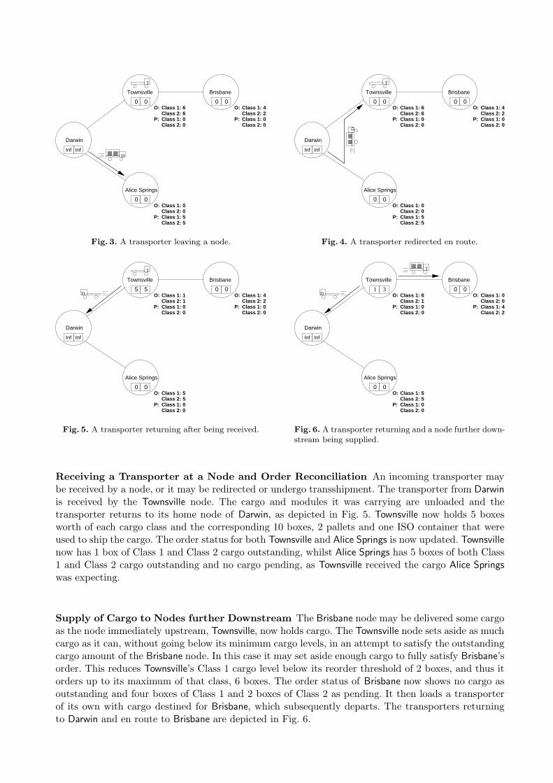
T

D

Class 1:Class 2:Class 1:Class 2:

O:

P:


O:

P:


O:

P:

Alice Springs

Darwin

Townsville Brisbane

0 0 0

00

0

Inf Inf

00

00

00

55

66

42

Fig. 3. A transporter leaving a node.

T

D


O:

P:


O:

P:


O:

P:

Alice Springs

Darwin

Townsville Brisbane

0 0 0

00

0

Inf Inf

00

00

00

55

66

42

Fig. 4. A transporter redirected en route.

D Class 1:Class 2:Class 1:Class 2:

O:

P:


O:

P:


O:

P:

T

Alice Springs

Darwin

Townsville Brisbane

0 0

00

Inf Inf

5500

100

5 51

00

42

Fig. 5. A transporter returning after being received.

T

D Class 1:Class 2:Class 1:Class 2:

O:

P:


O:

P:


O:

P:

Alice Springs

Darwin

Townsville Brisbane

0 0

00

Inf Inf

5500

6100

0042

1 3

Fig. 6. A transporter returning and a node further down-stream being supplied.

Receiving a Transporter at a Node and Order Reconciliation An incoming transporter maybe received by a node, or it may be redirected or undergo transshipment. The transporter from Darwin

is received by the Townsville node. The cargo and modules it was carrying are unloaded and thetransporter returns to its home node of Darwin, as depicted in Fig. 5. Townsville now holds 5 boxesworth of each cargo class and the corresponding 10 boxes, 2 pallets and one ISO container that wereused to ship the cargo. The order status for both Townsville and Alice Springs is now updated. Townsville

now has 1 box of Class 1 and Class 2 cargo outstanding, whilst Alice Springs has 5 boxes of both Class1 and Class 2 cargo outstanding and no cargo pending, as Townsville received the cargo Alice Springs

was expecting.

Supply of Cargo to Nodes further Downstream The Brisbane node may be delivered some cargoas the node immediately upstream, Townsville, now holds cargo. The Townsville node sets aside as muchcargo as it can, without going below its minimum cargo levels, in an attempt to satisfy the outstandingcargo amount of the Brisbane node. In this case it may set aside enough cargo to fully satisfy Brisbane’sorder. This reduces Townsville’s Class 1 cargo level below its reorder threshold of 2 boxes, and thus itorders up to its maximum of that class, 6 boxes. The order status of Brisbane now shows no cargo asoutstanding and four boxes of Class 1 and 2 boxes of Class 2 as pending. It then loads a transporterof its own with cargo destined for Brisbane, which subsequently departs. The transporters returningto Darwin and en route to Brisbane are depicted in Fig. 6.

3 Model Description

Although the example in Section 2.6 may seem simple, it will be seen that the model of the componentsthemselves is comprehensive and the generic nature of the model allows large logistics networks to beinstantiated. The modelling tool Design/CPN [7] was chosen as the computer tool with which thismodelling work would be undertaken. The primary rationale was that Design/CPN provided integratedstate space visualisation facilities and simulation-based performance analysis (although the latter isnow also supported by CPN Tools [5]), and that automated support exists for the translation of aDesign/CPN model to CPN Tools. This section introduces the architectural design philosophy used,the modelling scope and assumptions, and finally introduces the CPN model itself.

3.1 Architectural Design

During the development of our logistics network CPN we attempted to incorporate the followingdesirable features of a high-level architectural design. Extensibility : the design should allow for easyaddition of detail and extensions to the model. Modularity : well-defined interfaces between componentsallow components to be developed independently and aids extensibility. Precision: the architecturemust accurately reflect the real-life system, to an appropriate level of abstraction. Future-proofing : thearchitecture should guard against possible future changes to the greatest extent possible.

There were two main trade-offs that we considered during the development of our model. The firstwas Compactness versus Readability and Understandability , which incorporates trade-offs in visualisa-tion of control flow and data flow, model size, extensibility, ease of debugging and ease of maintenance.The second was Generality versus Specificity . A very specific model of a particular scenario may notbe so easily adapted to other scenarios. However, a very general model may capture too much and betoo difficult to analyse. This also relates to the flexibility of the model.

Nodes and links can be considered as relatively static objects, which could be considered as pro-

cesses. Transporters, on the other hand, traverse links and move from one node to another. We thereforemodelled nodes and links as (substitution) transitions, and transporters as tokens that traverse theCPN model. Interfaces between nodes and links contain information, and are modelled as shared places.

The logistics network CPN model underwent many changes during its development [9]. Here wejust discuss the representation of network topology. The topology was encoded in tokens, resultingin generic node and generic link pages as ‘execution engines’. This architectural design allowed themodelling of any topology without requiring structural changes to the model, as node and link additionsare accomplished by the addition of tokens. This facilitates modelling dynamic topology changes ‘on-the-fly’, for example the unavailability of a given inter-nodal link for a temporary period could bemodelled through token manipulation. A further advantage was the creation of a compact model, atthe cost of losing the ability to visualise the network topology (i.e. net elements such as substitutiontransitions corresponding directly to nodes or links). This meant that the number of model pagesremained the same as nodes and links were added, compared with a combinatorial explosion of pagesif the topology was modelled using net structure.

3.2 Modelling Scope and Assumptions

The model complexity was reduced to only that required to represent the behaviour of interest. Wehave abstracted from both the information network and the control mechanisms and embedded as littlecontrol in the model as possible, with a view to creating a model of the physical network as a test-bed for evaluation of particular control strategies. We have assumed that the information network isperfect, in that the knowledge that nodes have about each other is correct and updated instantaneouslyfor all nodes.

For the initial modelling work documented in this paper, we have only considered a pull (demanddriven) procedure for the distribution of assets, whereby downstream nodes request assets from up-stream nodes. We do not consider a push procedure or anticipatory logistics, where upstream nodesdirect assets to be sent to downstream nodes.

Nodes Storage area capacity and stock level characteristics were identified as the most relevant andimportant for our initial model of a node, as they are necessary for measuring effectiveness and per-formance. As previously discussed, we consider each node to have a maximum stock level, a minimumstock level, and a reorder threshold for each class of cargo modelled. In addition, we have modelledthe following 6 activities identified as the core activities of a node:

– Send: a node sends a transporter carrying cargo to another node.– Receive: a node receives a transporter (empty or carrying cargo) from another node.– Transship: cargo is moved from one transporter to another.– Redirect: transporters are directed away from this node towards an another node.– Consumption: supplies are consumed within a node.– Reordering: supplies are requested when the stock levels of one or more classes of supply fall

below a predetermined level (the reorder threshold).

Transporters The maximum payload (both volume and weight), the maximum weight of specifictransporters (both loaded and unloaded), and the maximum speed and range of a transporter wereconsidered to be important for our initial model. The maximum volume of payload is specified in termsof modules (see below). We define a home node for each transporter, as the node where it resides whenit is idle. We do not consider landing/docking/loading/unloading characteristics of transporters, inline with our modelling assumptions and scope for the modelling of nodes. We also do not considerthe breakdown (failure) of transporters in this initial model.

Links We consider links to be either unidirectional or bidirectional, and if bidirectional, half-duplex(allowing one direction of travel at a time) or full duplex (allowing travel in both directions simulta-neously). We consider the link characteristics to be the broad description (e.g. Sea, Air, Road, Rail),length, and maximum traversal speed only. The following link behaviours are included in our model:

– Successful traversal of the link;– Redirect en-route, where a transporter changes its destination and is directed towards another

destination, provided the eligibility requirements of the transporter and link are met; and– Return, where a transporter returns to its origin without traversing the entire link.

We make the assumption that the flow of supplies are acyclic. This allows for an unambiguousdefinition of an upstream and downstream direction over each link, as introduced in Section 2. We alsomake the assumption that the topology is static.

In addition, the domain of each transporter is restricted to be its home node and all nodes imme-diately downstream of its home node (i.e. the nodes directly supplied by the home node). This reflectsthe assumption that we are only considering a pull (demand) driven logistics system, in which it isonly possible for orders to be satisfied by the nodes immediately (one hop) upstream from the orderingnode. Hence, the movement of transporters is restricted to only one node downstream.

Cargo Cargo and supplies have been considered in an abstract way. In this example we consider onlytwo distinct classes of cargo, rather than 9. We did not abstract to a single class of cargo, as we wishedto keep in mind the implications for extending the model to cover more than two classes of cargo.Modelled characteristics of cargo include the cargo class and the cargo weight (density).

Modules We assume that each pallet can carry a maximum of 12 boxes, and that each ISO shippingcontainer can hold a maximum of 20 pallets or 20 ∗ 12 = 240 boxes (without pallets). It was notimportant to keep track of empty boxes, but we do keep track of empty pallets and ISO shippingcontainers. We assume that all cargo is boxed, for simplicity.

As mentioned in Section 2.4, there are numerous rules and restrictions on the classes of cargo thatcan be packed and stored together. Given that we only model two classes of cargo, we abstract from

GlobalDeclarations#2

Hierarchy#10010

Links#7 M Prime

Unidirectional_Link#15

Redirect#19

Transship#16

Receive#25

Send#26

Generic_node#43

Nodes#1 M Prime

Reorder#3

Consume#4

Initialisation#5 M Prime

Node_Internals

Send

Receive

Redirect

Transship

Link_Internals

Consume

Reorder

Fig. 7. Model Hierarchy.

these rules and restrictions by considering a policy of cargo segregation at the level of the pallet. Asin the example, when packing cargo into modules, we have followed the principle that if two or moremodules of the same size are included in a load then they must be loaded on/in a larger module (butonly without violating cargo segregation).

3.3 Model Description

The hierarchy page, shown in Fig. 7, gives an overview of the architecture of the model. The modelcontains 11 pages (excluding the hierarchy and global declarations pages), 69 places (including portand socket places and separate instances of fusion places), 8 substitution transitions, and 13 concretetransitions. This only tells part of the story, as substantial complexity is modelled in the inscriptionsdue to the high degree of folding in this model.

The model is divided into two sections, one with the Nodes page at the head modelling logisticsnodes, and the other with the Links page at the head modelling inter-nodal links. The hierarchicalstructure of pages modelling nodes has three layers. At the third layer, six pages represent the sixactions identified as core actions of a node: Redirect, Transship, Receive, Send, Reorder and Consume.The hierarchical structure of pages modelling links is much simpler, with only one page at each of thetwo hierarchical levels.

Separate from the node and link pages are two other pages: Global Declarations, which containsall the colour set definitions, variable declarations, and functions; and the Initialisation page which isused to populate the net with its initial marking. This design allows for the population of places inthe net with a pseudo-initial marking via functions rather than through an explicit hard-coded initialmarking. Modification of this pseudo-initial marking is possible by editing the function declarationsof the Global Declarations page rather than editing the net pages directly. Using functions in this wayfor the initial marking provides a mechanism where, in the future, the model can be populated witha particular scenario from an external source, e.g. a file or a Transmission Control Protocol (TCP)connection. Due to space limitations, we will describe the Nodes page and some of its subpages, butnot the Links or Unidirectional Link pages. Details of these pages can be found in [9].

Node_Internals

HS

Interface

TransportMode

FG

NetworkTopology

LinkChars

FG3

1‘(("Darwin","Alice Springs"),{maxSpeed = 100,maxWeight = 100000,distance = 499,medium = road},(true,0,"initially_none"))++ 1‘(("Darwin","Townsville"),{maxSpeed = 100,maxWeight = 100000,distance = 499,medium = road},(true,0,"initially_none"))++ 1‘(("Townsville","Brisbane"),{maxSpeed = 100,maxWeight = 100000,distance = 499,medium = road},(true,0,"initially_none"))

Idle_Transporters

NodexTransporter

FG

2

1‘("Darwin",{transportertype = type1,speed = 100,maxPayload = 22000,tareWeight = 11000,range = 500,medium = road,capacities = [{NumBoxes = 0,NumPallets = 0,NumISOs = 1}],home = "Darwin"})++ 1‘("Townsville",{transportertype = type2,speed = 100,maxPayload = 22000,tareWeight = 11000,range = 500,medium = road,capacities = [{NumBoxes = 0,NumPallets = 6,NumISOs = 0}],home = "Townsville"})

Modules_Store

NodexModules

FG

4

1‘("Alice Springs",{NumBoxes = 0,NumPallets = 0,NumISOs = 0})++ 1‘("Brisbane",{NumBoxes = 0,NumPallets = 0,NumISOs = 0})++ 1‘("Darwin",{NumBoxes = 0,NumPallets = 0,NumISOs = 0})++ 1‘("Townsville",{NumBoxes = 0,NumPallets = 0,NumISOs = 0})

NodeCharacteristics

NodeChars

FG4

1‘{node = "Alice Springs",send = true,receive = true,redirect = true,transship = true,consume = true,produce = false,stock = ({Class1 = 5,Class2 = 5},{Class1 = 0,Class2 = 0},{Class1 = 2,Class2 = 2})}++ 1‘{node = "Brisbane",send = true,receive = true,redirect = true,transship = false,consume = true,produce = false,stock = ({Class1 = 4,Class2 = 2},{Class1 = 0,Class2 = 0},{Class1 = 2,Class2 = 1})}++ 1‘{node = "Darwin",send = true,receive = true,redirect = true,transship = true,consume = false,produce = true,stock = ({Class1 = 10,Class2 = 10},{Class1 = 0,Class2 = 0},{Class1 = 5,Class2 = 5})}++ 1‘{node = "Townsville",send = true,receive = true,redirect = true,transship = true,consume = true,produce = false,stock = ({Class1 = 6,Class2 = 6},{Class1 = 1,Class2 = 1},{Class1 = 2,Class2 = 2})}

Cargo_Store

NodexCargo

FG

4

1‘("Alice Springs",{Class1 = 0,Class2 = 0})++ 1‘("Brisbane",{Class1 = 0,Class2 = 0})++ 1‘("Darwin",{Class1 = 0,Class2 = 0})++ 1‘("Townsville",{Class1 = 0,Class2 = 0})

Cargo_Orders

Order

FG5

1‘pullOrder(("Alice Springs",{Class1 = 0,Class2 = 0},{Class1 = 0,Class2 = 0}))++ 1‘pullOrder(("Brisbane",{Class1 = 0,Class2 = 0},{Class1 = 0,Class2 = 0}))++ 1‘pullOrder(("Darwin",{Class1 = 0,Class2 = 0},{Class1 = 0,Class2 = 0}))++ 1‘pullOrder(("Dummy",{Class1 = 0,Class2 = 0},{Class1 = 0,Class2 = 0}))++ 1‘pullOrder(("Townsville",{Class1 = 0,Class2 = 0},{Class1 = 0,Class2 = 0}))

Empty_Modules

NodexModules

FG

4

1‘("Alice Springs",{NumBoxes = 0,NumPallets = 0,NumISOs = 0})++ 1‘("Brisbane",{NumBoxes = 0,NumPallets = 0,NumISOs = 0})++ 1‘("Darwin",{NumBoxes = 0,NumPallets = 0,NumISOs = 0})++ 1‘("Townsville",{NumBoxes = 0,NumPallets = 0,NumISOs = 0})

ConsumptionProfile

ConsumptionProfile

FG1

1‘(true,[("Townsville",{Class1 = 2,Class2 = 3}),("Alice Springs",{Class1 = 2,Class2 = 3}),("Brisbane",{Class1 = 2,Class2 = 1})])

Fig. 8. The Nodes Page.

Node Hierarchy The top-level page of the node hierarchy, the Nodes page from Fig. 7, is shown inFig. 8. The Node Internals substitution transition interacts with a set of places described below. Themarking shown is the initial marking corresponding to the illustrative example from Section 2.6.

Node Characteristics Each individual logistics node is represented by a token in the Node Character-

istics place. The associated colour set, NodeChars, is defined as a record on lines 13 to 21 in Listing 1.

The ‘node’ field (line 14) is typed by the colour set, NodeID (lines 1 and 2), which defines a subsetof strings constituting legal names for the physical nodes. The last string of the subset, initially none,is used as the initial transporter direction on an inter-nodal link.

The six boolean fields (lines 15 to 20) denote whether a specific node can perform the correspondingfunctions of sending, receiving, redirection, transshipping, consumption or production of cargo. Thesefields are used as an enabling mechanism implemented via transition guards. This structure allows forthe creation of nodes which may only perform a limited number of functions, such as transshipmentnodes that do not hold cargo of their own, as well as providing the ability to alter node functionality‘on-the-fly’ simply by changing the boolean values in the corresponding token.

Finally, the ‘stock’ field (line 21), typed by the StockLevels colour set (lines 8 to 11), specifies themaximum, minimum, and reorder levels for cargo held at the node. These three levels are typed bythe Cargo colour set (lines 4 to 6), which is a record consisting of two integers representing the numberof boxes of each of two classes of cargo.

Network Topology The Network Topology place contains information regarding the inter-nodal linksof the model. Each token in this place represents the information for one link joining a pair of nodes,and is typed by the colour set LinkChars, shown on lines 18 to 21 of Listing 2.

The LinkID colour set (lines 1 to 3) is a product of two node IDs, defining a pair of nodes joinedby a link. The first node of the product is interpreted by the model as being one level upstream of the

Listing 1. Colour set Declarations for the Node Characteristics place.

1 c o l o r NodeID = subse t STRING with [" Darwin "," Townsville "," Brisbane "," Alice Springs ",

2 "initially_none"];

3

4 c o l o r Cargo = r eco rd

5 Class1 : INT *

6 Class2 : INT ;

7

8 c o l o r StockLevels = product

9 Cargo * (∗ Max Stock Leve l s ∗)

10 Cargo * (∗ Min Stock Leve l s ∗)

11 Cargo; (∗ Reorder Threshold ∗)

12

13 c o l o r NodeChars = r eco rd

14 node : NodeID * (∗ The node with these c h a r a c t e r i s t i c s ∗)

15 send : BOOL * (∗ Node can send ∗)

16 receive : BOOL * (∗ Node can r e c e i v e ∗)

17 redirect : BOOL * (∗ Node can r e d i r e c t ∗)

18 transship : BOOL * (∗ Node can t r an s sh i p ∗)

19 consume : BOOL * (∗ Node can consume cargo ∗)

20 produce : BOOL * (∗ Node can produce cargo ∗)

21 stock : StockLevels ; (∗ Max, Min and Reorder Threshold ∗)

Listing 2. Colour set Declarations for the Network Topology place.

1 c o l o r LinkID = product

2 NodeID * (∗ source / de s t i n a t i on ∗)

3 NodeID ; (∗ de s t i na t i on / source ∗)

4

5 c o l o r LinkType = with air | rail | sea | road;

6

7 c o l o r LinkInfo = r eco rd

8 maxSpeed : INT * (∗ Max speed o f t h i s l i n k ∗)

9 maxWeight : INT * (∗ Max weight o f t h i s l i n k ∗)

10 distance : INT * (∗ l ength ( d i s t an c e ) o f t h i s l i n k ∗)

11 medium : LinkType ; (∗ The medium of t h i s l i n k ∗)

12

13 c o l o r LinkDirectionSynch = product

14 BOOL * (∗ f u l l duplex ( t rue ) or h a l f duplex ( f a l s e ) ∗)

15 INT * (∗ number in t r a n s i t ∗)

16 NodeID ; (∗ l a s t d e s t i n a t i on / d i r e c t i o n o f f low ∗)

17

18 c o l o r LinkChars = product

19 LinkID * (∗ i d e n t i f e r f o r t h i s l i n k ∗)

20 LinkInfo * (∗ the c h a r a c t e r i s t i c s o f t h i s l i n k ∗)

21 LinkDirectionSynch; (∗ Di r e c t i on synch ron i s a t i on in fo rmat ion ∗)

second node. The LinkInfo colour set (lines 7 to 11) specifies the characteristics of the link, where thetransport medium is described by the enumerated colour set, LinkType, on line 5. These characteristicsdefine the eligibility criteria for transporters to traverse this link. The LinkDirectionSynch colour set(lines 13 to 16) provides a means of coordinating the directions of link traversal and enforcing traversalin one direction at a time for half-duplex links.

Interface The node and link pages of the model interact via the Interface place, typed by the Trans-

portMode colour set shown on lines 25 to 26 in Listing 3. A TransportMode token specifies a transporter(laden or unladen) entering or leaving a given node. The Transporter field specifies an individual trans-porter. The Transporter colour set (lines 10 to 18) is a record specifying a TransporterType (line 6),which may be thought of as a transporter descriptor, as well as a number of characteristics specific to

Listing 3. Colour set Declarations for the Interface place.

1 c o l o r Modules = r eco rd

2 NumBoxes : INT *

3 NumPallets : INT *

4 NumISOs : INT;

5

6 c o l o r TransporterType = with type1 | type2 | type3;

7

8 c o l o r Capacity = l i s t Modules ;

9

10 c o l o r Transporter = r eco rd

11 transportertype : TransporterType *

12 speed : INT *

13 maxPayload : INT *

14 tareWeight : INT *

15 range : INT *

16 medium : LinkType *

17 capacities : Capacity *

18 home : NodeID ;

19

20 c o l o r Load = product Modules * Cargo * NodeID ;

21 (∗ I n c l ud e s Or i g i na l Des t inat ion ∗)

22

23 c o l o r Direction = with outgoing | in_transit | incoming | returning ;

24

25 c o l o r TransportMode = product Transporter * Load * NodeID * NodeID * Direction ;

26 (∗ Transporter , Load , Source , Dest inat ion , D i r e c t i on ∗)

Listing 4. Colour set Declarations for Cargo Orders.

1 c o l o r PullOrder = product

2 NodeID * (∗ The node which generated the order / reques t ed the s upp l i e s ∗)

3 Cargo * (∗ The s upp l i e s r eques t ed that are not yet on t h e i r way

4 ( outstanding but not pending ) ∗)

5 Cargo; (∗ The s upp l i e s that have been sent but have not yet a r r i v ed ( pending ) ∗)

6

7 c o l o r Order = union pullOrder :PullOrder ; (∗ A union , f o r future−proo f i n g aga i n s t

8 other types o f o rder s / supply schemes ∗)

that individual transporter, including speed (for use in future performance analysis), maximum weightof payload, unloaded (tare) weight, range, and the medium via which the transporter can travel. Thecapacities field, typed by colour set Capacity (line 8), is a list of records of type Modules (lines 1 to 4),and details the possible maximum legal module configurations (there may be more than one) whichmay be loaded onto the transporter, thus giving the volumetric limitations of the transporter. Forexample, a truck may be able to carry either at most one ISO container or 10 pallets outside an ISOcontainer. Finally, the home field specifies the home location of the transporter.

The second element in the TransportMode colour set is the Load (lines 20 and 21). It specifies thenumber of boxes of each cargo class, the modules used to pack this cargo, and the original destinationof the particular load. This last field is necessary to keep track of the original destination of the cargo,for order reconciliation when a transporter is redirected.

The two NodeID terms of the TransportMode colour set define the current origin and destinationnodes of the transporter. The Direction term (defined on line 23) specifies whether the transporter isoutgoing, in transit, incoming, or returning. This is used by the model to determine the eligible actionsof the transporter when arriving at or departing a node, or when in transit.

Cargo Orders The Cargo Orders contains tokens representing the current order information for eachnode. It is typed by colour set Order, (line 7 of Listing 4) which corresponds to a PullOrder (lines 1

Listing 5. Colour set Declarations for Consumption Profile and Cargo Store.

1 c o l o r NodexCargo = product NodeID * Cargo;

2 c o l o r NodexCargoList = l i s t NodexCargo ;

3 c o l o r ConsumptionProfile = product BOOL * NodexCargoList;

Listing 6. Colour set Declarations for Modules Store, Empty Modules and Idle Transporters.

1 c o l o r NodexModules = product NodeID * Modules ;

2 c o l o r NodexTransporter = product NodeID * Transporter ;

to 5) in our current model. PullOrder comprises: the identifier of the node placing the order (NodeID);the amount of cargo outstanding; and the amount of cargo pending (both of type Cargo).

Consumption Profile The declarations for the Consumption Profile place, which holds a list detailingthe cargo consumption information for the nodes, is shown in Listing 5. This consumption profile (line2) is modelled as a list of pairs (line 1): the node (NodeID) at which consumption occurs and the amountof cargo to be consumed (Cargo) in a particular consumption event. Thus cargo consumption proceedsby stepping through the elements in this list. This list is paired with a boolean in the ConsumptionProfile

colour set (line 3) which specifies whether the consumption profile cycles, i.e. the consumption eventsin the consumption profile repeat from the start when the end of the profile is reached.

Cargo Store, Modules Store, Empty Modules and Idle Transporters Cargo Store contains tokensrepresenting a stock level (line 1 of Listing 5). Similarly, Modules Store and Empty Modules describethe numbers of modules currently being used to store cargo and empty modules, respectively (line 1of Listing 6). Idle Transporters contains transporters that are available for use (line 2 of Listing 6). Inthe colour sets of all four places, the NodeID specifies where the cargo, modules and transporter arecurrently situated.

The Generic node Page and Structure The Generic node page, shown in Fig. 9, shows the in-teractions of the logistics functions Send, Receive, Transship, Redirect, Consume and Reorder. Each ofthese logistics functions is represented on this page by a substitution transition. All of the substitutiontransitions are connected by bidirectional arcs to the Node Characteristics place, as all actions requireknowledge of the node characteristics.

The substitution transitions that model actions in which a transporter enters or leaves a node,Redirect, Receive, Transship, and Send, are all connected to the Interface place. A transporter enteringa node may be received, redirected, or transshipped. A transporter that is received or transshippedwill return to its home node if its current location is not its home. Also, the send action will result in atransporter leaving the node. Therefore, the arcs connecting the Interface place to the Receive, Redirect

and Transship actions are bidirectional, whereas there is only an arc from Send to Interface, and notvice versa. These four actions that deal with transporters entering or leaving a node are connectedby bidirectional arcs to the Network Topology place, to obtain the required information describing thenetwork topology.

The Receive action may result in a transporter becoming idle (if the receiving node is its homenode), hence the arc from Receive to Idle Transporters. The Transship action will require the use of idletransporters and may result in a transporter becoming idle (if the transshipping node is the home nodeof the incoming transporter), hence the bidirectional arc between Transship and Idle Transporters. TheSend action requires idle transporters, hence the arc from Idle Transporters to Send.

The Cargo Store and Modules Store places are connected to both the Send and Receive actions, asthe former results in a reduction in the cargo and modules held at a node, while the latter results inan increase of the amount of modules or the amount of modules and cargo in a node. The Transship

Transship

HS

Interface

P I/O

TransportMode

Redirect

HS

Idle_Transporters

NodexTransporter

P I/O

Receive

HS

Send

HS

Modules_Store

NodexModules

P I/O

NetworkTopology

LinkChars

P I/ONodeCharacteristics

NodeChars

P I/O

Cargo_Store

NodexCargo

P I/O

Consume

HS

Cargo_Orders

Order

P I/O

Reorder

HS

Empty_Modules

NodexModules

P I/O

ConsumptionProfile

ConsumptionProfile

P I/O

Fig. 9. Generic node page.

action, however, is only connected to the Modules Store place, as cargo for transshipping is modelledinternally on the Transship page. Receive and Transship are connected to the Empty Modules place, asempty modules may be loaded onto transporters returning to their home node from receive or transshipactions.

Cargo consumption is modelled by Consume, resulting in additional empty modules being producedand a reduction in the amount of cargo and the number of modules packed with cargo in the node.The existing amount of cargo and number of modules must be known, hence there are bidirectionalarcs between Consume and the Cargo Store, Modules Store and Empty Modules places, to read theserecords and then update them.

The Reorder substitution transition needs to know the current cargo holdings of the node, hencethe bidirectional arc between Reorder and Cargo Store. A node’s order token is updated, hence thebidirectional arc between Reorder and Cargo Orders. Due to the order-driven nature of the modelledsystem, the Send and Receive actions also have bidirectional arcs to Cargo Orders.

The Send action attempts to supply the required cargo to satisfy the order of a downstream node,decreasing the outstanding cargo and increasing the pending cargo of the downstream node. TheReceive action reconciles orders and cargo, reducing the cargo pending (if the receiving node has cargopending of the corresponding class(es)) and possibly increasing the cargo outstanding of the originaldestination (if the receiving node is not the original destination).

Outgoing_Cargo

NodexNodexCargo

FG

Outgoing_Cargo

Assign_Cargo

[(#send nodeChars) andalso thisNode2=(#2 linkID) andalso thisNode <> thisNode2 andalso thisNode = (#node nodeChars) andalso thisNode = (#1 linkID) andalso cargoSize(cargoOutstanding)>0 andalso ((if(#Class1 cargoOutstanding > 0) then (#Class1 cargo > 0) else true andalso if(#Class2 cargoOutstanding > 0) then (#Class2 cargo > 0) else true) orelse (#produce nodeChars))]

C

NetworkTopology

LinkChars

P I/O

NodeCharacteristics

NodeChars

P I/O

Cargo_Store

NodexCargo

P I/O

Cargo_Orders

Order

P I/O

Idle_Transporters

NodexTransporter

P In

Modules_Store

NodexModules

P I/O

Interface

TransportMode

P Out

Pack_Load_Send

C[(#node nodeChars) = thisNode andalso thisNode = (#1 linkID) andalso thisNode2 = (#2 linkID) andalso cargoSize(cargo) > 0]

(thisNode,thisNode2, {Class1= (#Class1 cargo1) + class1a, Class2 = (#Class2 cargo1) + class2a})

(linkID, linkInfo,synchInfo)nodeChars

1‘(thisNode, if(#produce nodeChars) then cargo else {Class1 = (#Class1 cargo)-class1a, Class2 = (#Class2 cargo)-class2a})

(thisNode,cargo)pullOrder(thisNode2, {Class1=(#Class1 cargoOutstanding)-class1a, Class2=(#Class2 cargoOutstanding)-class2a}, {Class1=(#Class1 cargoPending)+class1a, Class2=(#Class2 cargoPending)+class2a})

pullOrder (thisNode2,cargoOutstanding, cargoPending)

(transporter,(modulesPacked, cargoPacked,thisNode2), thisNode, thisNode2, outgoing)

(thisNode,transporter)

(thisNode,modulesRemaining)(thisNode,modules)

(thisNode,thisNode2,cargo) (thisNode,thisNode2,cargoRemaining)

(linkID, linkInfo, synchInfo)

(thisNode, thisNode2,cargo1)

nodeChars

Fig. 10. Send page.

Due to space limitations we shall only describe one page at the third level. This is the Send page,corresponding to the substitution transition of the same name on the Generic node. Details of the othersub-pages can be found in [9].

Send Page The Send page, shown in Fig. 10, models the logistics function of sending cargo packed inmodules on a transporter bound for a downstream node to fulfill an order from that downstream node.The send function is divided into two phases represented by the Assign Cargo and Pack Load Send

transitions.The first (Assign Cargo) sets aside cargo in response to an order. A code segment (not shown in

Fig. 10) is used to calculate the amount of cargo to put aside for delivery to an immediate downstreamnode, based on the current stock levels and the outstanding cargo amount in the order from thecorresponding downstream node. The assigned cargo is placed in Outgoing Cargo and labelled with itsintended destination.

The second (Pack Load Send) packs the previously set-aside cargo bound for one particular desti-nation into modules and loads them onto a transporter. This also makes use of a code segment (againnot shown) to calculate the maximum amount of cargo (and necessary modules for packing) that canbe loaded onto a nondeterministically chosen idle transporter residing at the sending node. The codesegment must take into account the weight and volumetric capacity of the transporter, the weightrestrictions of the outgoing link, the policy of cargo segregtion (to keep classes of cargo segregatedat the pallet level) and the packing procedure (two or more of any module must reside on or in a

larger module, if it exists). The cargo and modules to be packed (and the cargo and modules left over)are calculated by incrementally adding boxes of cargo to the load of the transporter until one of theconstraints is reached, or it runs out of cargo or modules. The motivation for using a code segment tocalculate this amount of cargo is discussed in Section 4.4.

4 Discussion

During the course of the modelling work, we discovered a number of limitations of the modelling tools,Design/CPN and CPN Tools, as well as encountered difficulties with the use of CPNs as the modellingformalism for such a system. These difficulties, and their solutions, are discussed below.

4.1 Handling of Large Models

Early in the model’s evolution, the topology of the logistics network was represented explicitly in thenet structure, resulting in a large number of pages (around 30 to 35). We experienced difficulties in usingthe Design/CPN editor. The tool would sometimes not allow us to add, edit or remove net elements(places and transitions). Sometimes it would not save nets correctly and would crash when loadingthem. This problem disappeared after reducing the number of pages in the model by representing thetopology in tokens.

4.2 Extensible Data Structures

Significant effort went into designing data structures for the model. For example, for cargo, we con-sidered a list, a product and a record. Lists have the advantage of extensibility, in that the numberof elements in the list (the list length) is not hard-coded into the data structure itself. Thus, in thefuture, the number of classes of cargo can be extended without changes to the corresponding colour setdefinition. However, lists suffer from a significant disadvantage, namely the additional programmingeffort required to ensure the model maintains a coherent and meaningful list structure and ordering.

Products and record structures to not suffer from this disadvantage, as the structure is implicit inthe colour set itself and no additional effort is needed to maintain this structure. Although productsand records have essentially the same underlying data structure, records provide more informationto the user regarding exactly what element is being accessed, through explicit field labels. For thesereasons, records were chosen. The downside of using records is that arc inscriptions become very large,as each field of the record must be explicitly represented in inscriptions if a new token of this recordtype is to be created, even if values from an existing token are being reused. An example of this canbe seen on the arc from the Assign Cargo transition to the Cargo Orders place in Fig. 10. Anotherdisadvantage of both products and records is that they lack the extensible nature of lists, due to theirstatically defined structure, thus any addition to the number of cargo classes requires modification ofcolour sets, all related arc inscriptions, guards and code segments.

4.3 Excessive Nondeterministic Choice: Binding Element Explosion

An interesting problem that we faced was that of binding element explosion. One of the strengthsof the CPN formalism is its ability to handle concurrency and nondeterminism. When attemptingto model a logistics network with very abstract control mechanisms, our philosophy was to modelnondeterministically as many choices as possible, and so not ‘hard wire’ aspects of control into themodel, in order to capture all possibilities of physical actions. The explosion of binding elements becamea problem, most notably with the sending, ordering and consumption actions, as it became evidentthat the Design/CPN simulator cannot handle a large number of binding elements.

As an example, consider 10 boxes of each of 9 classes of cargo (90 boxes in total). When choosingnondeterministically a number of boxes (from 0 to 10) of each class to consume, this gives 11 choices foreach of the 9 classes, i.e. 119 possibilities (over 2.3 billion). The syntax check within Design/CPN was

successful and the simulator tool could be entered. However, attempts at both automatic and manualsimulation caused the tool to crash when attempting to calculate such large numbers of enabledbindings for the Order and Consume transitions. When attempts were made to bind the values ofvariables manually, the tool would also crash when attempting to display all choices to the user.

After converting the model to CPN Tools format and opening it in CPN Tools, it was discoveredthat CPN Tools also could not handle this situation. We believe that the reason is caused by themerging of the editor and simulator in CPN Tools. CPN Tools performs syntax checking on-the-fly,thus allowing the complete parts of a partially complete model to be simulated. In our case, however, theexcessive nondeterminism manifested itself as an excessively long syntax check that did not terminate(it was terminated manually after 40 minutes). The syntax check never advanced to the stage whereeven part of the CPN could be simulated.

This prompted us to seek a reduction in the degree of nondeterminism when choosing cargo to send,order or consume. Rather than allowing any amount of cargo to be sent from one node to another,we enforced a specific ‘packing policy’ by implementing an algorithm that determines the amount andconfiguration of cargo to be packed into a transporter and sent in the Pack Load Send action. This isdiscussed in more detail in Section 4.4 below.

The excessive nondeterminism introduced by the ordering mechanism, which allowed any nodeto order any amount of cargo, was curtailed by the introduction of the pull order mechanism. Eachnode was then able to determine specific amounts of cargo to order. The nondeterminism in cargoconsumption was alleviated by the introduction of consumption profiles, which dictate both what isto be consumed by each node and the ordering of consumption events over the consuming nodes.

4.4 The Use of Code Segments for Implementing Nondeterministic Constraints

Arc inscriptions and guards allow the specification of constraints that restrict the set of bindingelements enabled by a particular marking. These constraints are generally known and set staticallywhile creating the model, and a given binding of variables will either satisfy the constraints, or willnot satisfy the constraints. The term nondeterministic constraints refers to the situation in which theconstraints themselves are not explicitly known prior to run-time, and are determined by the valuesof the variables themselves in a given binding element.

Specifically, difficulties were encountered when attempting to load a transporter with cargo andmodules via the Pack Load Send operation. Our goal was to load as much cargo as possible (up to theamount of cargo set aside for one destination) while still conforming to the weight restrictions of theoutgoing link and the weight and volumetric capacity constraints of the transporter itself. Restrictingthe amount of cargo to satisfy the weight and capacity constraints listed above is not difficult and canbe achieved using conventional guard expressions. However, any binding element that satisfies theseconstraints is enabled. To force the amount of cargo to be ‘as large as possible’ within these constraintswas a more difficult task, and one that we could not achieve with guards and arc inscriptions alone.

This prompted the use of code segments to bind the cargoPacked and modulesPacked variables (andthe complementary cargoRemaining and modulesRemaining variables), based on the cargo available forsending, the transporter chosen, and the outgoing link. Due care must be taken when using codesegments to bind the values of variables so as not to result in illegal token colours. The method chosento calculate the values of the variables is as described under the Send page description at the endof Section 3.3, where the cargo (and required modules) is incrementally increased until one of theconstraints is reached. This guarantees that the cargo and modules sent never exceeds the amount ofavailable cargo and modules, the weight restrictions of the outgoing link, or the weight and volumetricconstraints of the transporter.

5 Conclusions

This paper presents a Coloured Petri Net model of a Defence Logistics Network capturing the principaloperations of a pull-based physical network, and some of our experiences in carrying out the modelling

activity. The modelling presented a significant challenge, due to the size and complexity of the domain.This paper describes the major physical components of a logistics network, the intuition behind themodel dynamics by means of a simple case study, and the detailed implementation of the operationsrelated to supplies.

The model has nodes, which represent military bases or staging points, and links between nodes asits major components. We discuss the scope of the model and some important assumptions, includingthe abstraction of the information network and the control mechanisms within the logistics networkmodel. More details, including a description of the model evolution, can be found in [9]. Care wastaken to build an accurate and precise model reflecting a real-world logistics network, to ensure theextensibility and modularity of the model, and to provide some measure of future-proofing of themodel. An important decision was to encode the network topology within CPN tokens rather than inthe net structure itself, to allow the model to be both flexible and adaptable to a range of networkimplementations. Without such an encoding, any change to the topology would require a change tothe net structure, whereas currently this only requires a change in the pseudo-initial marking. It alsomakes the CPN model much more compact and manageable, at the expense of losing a one-to-onemapping of net elements to physical entities, and hence reducing the readability and visualisation ofdata flow.

Our modelling work has also revealed a number of limitations of Design/CPN and CPN Tools. Mostof these relate to the operation of the simulator (in Design/CPN) and incremental syntax checkingand the state space tool in CPN Tools. This paper discusses the problems we encountered and ourapproach to overcoming them, while still achieving our original objectives.

Two key future work activities are immediately forthcoming from the work presented in this pa-per. The first is a continuation of the modelling of the functional behaviour of the logistics network.Many simplifications and assumptions were made to obtain the model in the time available. Thus thereis considerable scope for incremental relaxation of these assumptions, and for extensions and refine-ments to the model. This also includes the ongoing incorporation of feedback and suggestions fromdomain experts in the defence logistics area. Potential future modelling tasks include: the modellingof a realistic and imperfect information network; implementation of a mechanism to allow differentcontrol schemes to be imposed on the system; a more extensible implementation of cargo classes; morecomplete modelling of node, transporter and link characteristics; incorporation of transporter failures;more advanced routing schemes for transporters; more advanced delivery schemes, including milk-runs

(where a transporter delivers to multiple nodes in a single excursion) and aggregation of orders frommultiple downstream levels; the ability to represent more complex network topologies including cyclicnetworks; and a dynamically changing network topology. Importantly, incorporation of time into themodel would allow some quantitative results to be obtained.

Given our solutions for alleviating binding element explosion, our model runs successfully underboth Design/CPN and CPN Tools. Thus the second key future work activity is the formal analysisof such a model. This task can be divided into two parts. The first is functional analysis, whichmay consist of generation and analysis of the full or partial reachability graphs of the logistics CPNmodel. The second is performance analysis. This will require the identification and formulation ofa number of measures of performance that give quantifiable results to the measures of performancethat are of interest to DSTO. Such measures of performance may include module utilisation, averagestock levels, or the time spent below the minimum and/or reorder thresholds for each class of supply.Multiple simulation runs of the CPN model incorporating time, could then be undertaken to gaugeand compare the relative performance of different Logistics Network configurations.

Acknowledgments

The authors would like to acknowledge Greg Allen, Michael Burgess, Bruce Vandepeer and MAJ RobWebb for their valuable input and support throughout the course of this project.

References

1. W. M. P. van der Aalst. Timed Coloured Petri Nets and their Application to Logistics. PhD Thesis, EindhovenUniversity of Technology, 1992.

2. Australian Defence Doctrine Publication 4.0 - Defence Logistics. Defence Publishing Service, Department of Defence,8 April 2003.

3. J. Billington, M. Diaz, and G. Rozenberg, editors. Application of Petri Nets to Communication Networks, volume1605 of Lecture Notes in Computer Science. Springer-Verlag, 1999.

4. H. J. Bullinger and J. V. Steinaecker. Petri Net Based Modelling, Planning and Control of Logistical Processesunder Environmental Goals and Constraints. In Proc. of 9th Symposium on Information Control in Manufacturing,volume 1, pages 433–438. Elsevier Science, June 1998.

5. CPN Tools. http://wiki.daimi.au.dk/cpntools/cpntools.wiki.6. C. Degano and A. Di Febbraro. On using Petri Nets to Detect and Recover from Faulty Behaviours in Transportation

Facilities. In Proc. of the 2002 IEEE Int. Conf. on Systems, Man and Cybernetics, volume 1, pages 31–36. IEEE,Oct 2002.

7. Design/CPN Online. http://www.daimi.au.dk/designCPN/.8. I. Eick, D. Vogelsang, and A. Behrens. Planning Smelter Logistics: A Process Modeling Approach. In Light Metals

2001, New Orleans, LA, pages 393–398. Minerals, Metals and Materials Society, Feb 2001.9. G.E. Gallasch, N. Lilith, and J. Billington. A Coloured Petri Net Model of a Defence Logistics Physical Network.

Technical Report CSEC-25, Computer Systems Engineering Centre Report Series, University of South Australia,August 2006.

10. N. E. Hutchinson. An Integrated Approach to Logistics Management. Prentice-Hall, 1987.11. K. Jensen. Coloured Petri Nets: Basic Concepts, Analysis Methods and Practical Use. Vol. 1, Basic Concepts.

Monographs in Theoretical Computer Science. Springer-Verlag, 2nd edition, 1997.12. L.M. Kristensen, S. Christensen, and K. Jensen. The Practitioner’s Guide to Coloured Petri Nets. International

Journal on Software Tools for Technology Transfer, 2(2):98–132, 1998.13. L.M. Kristensen, B. Mitchell, L. Zhang, and J. Billington. Modelling and Initial Analysis of Operational Planning

Processes using Coloured Petri Nets. In Formal Methods in Software Engineering and Defence Systems 2002, Pro-ceedings of the Satellite Workshops on Software Engineering and Formal Methods and Formal Methods Appliedto Defence Systems, volume 12 of Conferences in Research and Practice in Information Technology Series, pages105–114. Australian Computer Society Inc., 2002.

14. B. Mitchell, L. M. Kristensen, and L. Zhang. Formal Specification and State Space Analysis of an OperationalPlanning Process. In Proceedings of the 5th Workshop and Tutorial on Practical Use of Coloured Petri Nets and theCPN Tools (CPN’04), Aarhus, Denmark., pages 1–18, 2004.

15. E. Ochmanska. Object-oriented PN Models with Storage for Transport and Logistic Processes. In Proc. of the 9thEuropean Simulation and Symposium, Passau, Germany, pages 483–487, San Diego, CA, USA, Oct 1997. SCS.

16. M. A. Piera, M. Narciso, A. Guasch, and D. Riera. Optimization of Logistic and Manufacturing Systems throughSimulation: a Coloured Petri net-based methodology. Simulation, 80(3):121–129, 2004.

17. The Technical Cooperation Program (TCCP). Guide for Understanding and Implementing Defence Experimentation(Guidex). Version 1.1, February, 2006.

18. US Department of Defense. Logistics Transformation Strategy - Achieving Knowledge-Enabled Logistics. 10th De-cember, 2006.

19. J. G. A. J. van der Vorst, A. J. M. Beulens, and P. van Beek. Modelling and Simulating Multi-echelon Food Systems.European Journal of Operational Research, 122(2):354–366, 2000.

20. N. Viswanadham and N. R. S. Raghavan. Performance Analysis and Design of Supply Chains: A Petri Net Approach.Journal of the Operational Research Society, 51(10):1158–1169, 2000.

21. M. von Mevius and R. Pibernik. Process Management in Supply Chains – A New Petri-net Based Approach. In Prof.of the 37th Annual Hawaii Int. Conf. on System Sciences, volume 37, pages 1153–1162. IEEE Computer Society, Jan2004.

22. Z. Wang, J. Zhang, and F. T. S Chan. A Hybrid Petri Nets Model of Networked Manufacturing Systems and itsControl System Architecture. Journal of Manufacturing Technology Management, 16(1):36–52, 2005.

23. Websters dictionary.24. L. Zhang, L.M. Kristensen, C. Janczura, G.E. Gallasch, and J. Billington. A Coloured Petri Net based Tool for

Course of Action Development and Analysis. In Formal Methods in Software Engineering and Defence Systems2002, Proceedings of the Satellite Workshops on Software Engineering and Formal Methods and Formal MethodsApplied to Defence Systems, volume 12 of Conferences in Research and Practice in Information Technology Series,pages 125–134. Australian Computer Society Inc., 2002.

25. L. Zhang, L.M. Kristensen, B. Mitchell, G.E. Gallasch, P. Mechlenborg, and C. Janczura. COAST - An OperationalPlanning Tool for Course of Action Development and Analysis. In Proceedings of the 9th International Commandand Control Research and Technology Symposium (ICCRTS), Copenhagen, Denmark, 2004.

Protos2CPN:Using Colored Petri Nets for Configuring and Testing

Business Processes

F. Gottschalk, W.M.P. van der Aalst, M.H. Jansen-Vullers, and H.M.W. Verbeek

Department of Technology Management, Eindhoven University of Technology,P.O. Box 513, 5600 MB, Eindhoven, The Netherlands.

[email protected]

Abstract. Protos is a popular tool for business process modelling used in more than1500 organizations. It has a built-in Petri-net-based simulation engine which shows keyperformance indicators for the modelled processes. Reference process models offered forProtos reduce modelling efforts by providing generic solutions which only need to beadapted to individual requirements. However, the user can neither inspect or inter-act with simulations running in Protos, nor does Protos provide any explicit supportfor the adaptation of reference models. Hence, we aim at a more open and config-urable simulation solution. To realize this we provide two transformations from Protosmodels to colored Petri nets (CPNs), which can be executed by CPN Tools. The firsttransformation enables the usage of the extensive simulation and measuring featuresof CPN Tools for the simulation of Protos models. The second transformation createscolored Petri nets with dedicated features for process configuration. Such configurableprocess models can be restricted directly within the process model without changingthe model’s structure and provide therefore dedicated adaptation features for Protos’reference process models.

1 Introduction

Today “process thinking” has become a mainstream organizational practice [20]. Businessprocess models provide a graphical and systematic view on organizational processes [15].Various tools for business process modelling have been developed since the late nineties [2].One popular tool is Protos from the company “Pallas Athena”. Currently it is used by about1500 organizations in more than 20 countries. E.g., more than half of all municipalities withinthe Netherlands use Protos for the specification of their in-house business processes [24].

Most providers of modelling tools, and, e.g., also all dominant enterprise system vendorsprovide reference models with or for their software. Reference models are supposed to reducethe modelling efforts by providing generic solutions that just need to be adapted to individualrequirements [5,9,10,11,18,19]. Pallas Athena provides several sets of reference process modelsimplemented in Protos. As an example, there is a set of about 60 reference process models formunicipalities. These are ordinary Protos models depicting common processes. The munici-pality or organization buying such a reference model can adapt the models to its individualrequirements, avoiding the huge effort of building process models from scratch. However, itis quite important to note that neither Protos nor any other popular process modelling toolprovides any explicit support for the adaptation of reference models [16].

Figure 1 depicts a reference process model for the handling of objections against parkingtickets1. If an objection is received within the corresponding deadline it is checked for its1 The model is motivated by one of Pallas Athena’s reference models, but specially build for the

purpose of this paper.

��

��

��

��

��

��

��

��

��

��

��

��

��

��

� ��

��

��

��

� ��

��

��!"��

��

��

#��

"��

��"��

$��!%�

��

��

��

%��

$��

#��

&��'

Fig. 1. An example decision-making process about objections against parkingfines, modelled in Protos

admissibility. In case it is not admissible, a supplement is requested. If this is received withinthe new deadline or if a supplement was not needed, the parking administration is consulted,reasons for approval/refusal as well as a settlement are drawn up, and the judgement is sentto the objecting citizen. Otherwise the objection times out and is refused directly as it is incase the objection was not received within the deadline.

During this research a set of more than 500 reference and adapted process models wasmade available to us by Pallas Athena. Although guidelines how to model sound businessprocesses in Protos and tools for verification exist [21,22,23], we discovered that most of theseprocess models do not conform to the guidelines. In addition, the models lack of data requiredfor process simulations which also means that simulation [24] was hardly used, if at all. So wecan conclude that the designers were either unaware or not convinced of the value of soundmodels and simulation. One main reason for this is that it is unclear to designers which of theparameters that can be specified in Protos are actually used for the simulation. For example,we discovered that in Protos a field for the number of resources required for the execution ofa task exists, but the simulation always uses just one resource and neglects this parameter.

Within this paper we will present two new tools helping Protos users to test and vali-date their process models and therefore to improve the quality. Both tools are available fordownload from http://www.floriangottschalk.de/protos2cpn.

First, we will depict a new way to simulate business processes modelled in Protos usingCPN Tools [25]. Nowadays CPN Tools is probably the most popular modelling and analysisenvironment for colored Petri nets (CPNs) [14], used in more than 115 countries with morethan 3000 licensees. It provides not only a nice way to visualize running processes but alsoextensive measurement and verification opportunities for concurrent systems. Within thisresearch we developed a transformation from Protos models to CPNs, using the same data asthe current Protos simulation. Using the simulation of CPN Tools we enable the unexperienceduser to see directly in which order the process tasks are executed and what might go wrong inincorrect workflow models. In additon some basic statistics are provided to him. The advanceduser will be able to add additional measurements to process models as well as he can seewhich of the Protos parameters are actually used during the simulation. The current Protossimulation is using a tool called ExSpect [4,24] which is based on another type of colored Petrinets. However, ExSpect does not allow for the easy creation of additional measurements. Itsstandard layout scheme, which is applied when loading a model, causes unacceptable delayswhen trying to inspect or interact with running processes. In addition, the development ofExSpect has stopped for some time already [12].

Second, we change the transformation in such a way that it creates a configurable pro-cess model from the Protos model. We developed configurable process models in our pre-vious research as a general mechanism for process model adaptation [5,13]. When config-uring a process, its unnecessary parts are eliminated, i.e. the possible process behavior isrestricted [9,10,18,19]. Incorporating configuration options into the process model during thetransformation creates for the first time a tool allowing to make process configuration deci-sions within a process model and to evaluate the configuration decision by direct interactionswith the simulation model.

The paper concludes with a summary and an outlook on open issues.

2 Protos2CPN: From Protos Models to Colored Petri Nets

Basically Protos2CPN converts the data provided by Protos for the current simulation into aCPN, executable in CPN Tools. So far, CPN Tools provides no opportunities for importingother file formats than the CPN Tools XML-file format. It is therefore reasonable to use anXML export of Protos and transform this into the CPN Tools format by an XSL transforma-tion. The current Protos simulation [24] is already using temporary stored XML files for thecommunication between Protos and ExSpect. So we decided to “plug-in” in between using thesame XML export for the generation of the CPN Tools files, especially as our main goal is theprocess simulation as well. The exported XML file includes a flattened process structure (i.e,the hierarchical structure is reduced to a single level process model), the resource utilizationof each task, and further statistical simulation parameters. It lacks of information how tolayout the process, but we aim at providing an automatic layout functionality. Currently, themodels are created with a basic layout scheme that allows for an easy re-arranging of processelements, keeping the manual effort reasonable.

In order to enable the user to look at the CPN in the same way as to the Protos model,without the need for learning a new “complicated” modelling language [17], it is our goalto transform the Protos models into CPN models that match the Protos model in look andstructure as close as possible. For that reason we decided that any information not depictedin the process view of Protos (cf. Figure 1) but maintained in property dialogues and neededfor simulation must be depicted on separate sub-pages. The derived CPN model provides

��

��

�� ! �� "��

��

#$��%��!��& � ��

� '!� ��

(�)*"�& �� * ��

� '!� ��

�� (� ��+� ��* ��

� '��

� '�� (�

� '�� (�

� '!� ��

� '!� ��

� ��)��,�% ��

� '!� ��

� '!� ��

� '��

� '!� ��

��

��

-.� � /�� 0��& � ��

'!/��1�2 �� *� � $��)*� ( �� 1�� & � � 3

�� 4�� 4

�� )�� #$�,�

�� $��4�� $��4

-.�� *� �� 5 ��,"�"�& �)*��

��*2 ��)*��

�� (��$�76�� (��$�76

�� & �)*��% �� (� ��

�� 89��"* �� & & �)*��

�� (��$�7:�� (��$�7:

;(�� <��"��

�� 8=��"* �� <� �� 5��"�"� ��>�& ?� �� &

�� (��$�� (��$��

@ �� *��)*� �, �� .�� & � ��

'!�� (��& �%"�� *��)��

�� A�� A

;B�C��,� ��%��%��)�� 1�& �

DE (�� $ ��"�"�& �)*��

�� F�� F

;B�C�� %��)*� � �� 1�& �

G�� H�� 0��

�� I�� I

;B�� 1�2 �(� � ��

�� (��$�7J�� (��$�7J

Fig. 2. The overall process view of the CPN (generated from the Protos processmodel depicted in Figure 1)

therefore two levels: First the overall process view, similar to the (flattened) process viewof Protos, where every Protos status2 is transformed into a CPN place3 and each Protostask is transformed to a CPN substitution transition (cf. figures 1 and 2); and second thesub-pages of these substitution transitions representing an “execution layer” incorporating alldata relevant for the simulation (cf. Figure 3).

2 The Protos name for a place (e.g., a model object representing a channel or state) is status.3 Note, that in Protos it is possible to connect transitions directly to transitions or statuses directly

to statuses whereas in (colored) Petri nets this is not. In this case additional auxiliary statuses ortransitions are introduced into the CPN process overview model. This is already done by Protoswhen creating the XML export.

��

� ��

� � ��

��

�� !� � � �� !� � � ��

"�# �� %$ ��& & ' ��( � � & & "

"�# �� %$ ��& & ' ��( � � & & "

( � ��

# ��%)

� �� +* � � � �, - , �� . � � ' ��, / ' 01�� 32 / ' 01��254�6 ��7 � � $�/ ' 0��4

� ��, � %$ ��8 ��

� . �� ' , ��9�, �+��

��

� ��

� � � ��

:;6 ��7 � � $�/ ' 01�

' ��< �� 254�=� �� < �� 2 ��7 � � $�/ ' 01��4�=�� %� ' ��12 7 � � $�/ ' 01� � .�>?25454�=

Fig. 3. Dedicated task page with information for simulation

The places in the overall model are allowed to have tokens of the type tCase4 depictingdetails about the cases running through the process, e.g., a case id, the start time of theprocess, and the arrival time of the process in the particular place:

colset tCase = record lCaseID:INT *lProcessArrivalTime:INT *lRank:INT *lPlaceArrivalTime:INT *lCost:INT;

Whenever a token is residing in one of the places in the overall model it is waiting forexecution by one of the subsequent transitions. All specifications of how and when a task canbe performed by one of these transitions are “hidden” on the corresponding sub-page for thetask, i.e. the transition depicted in the overall model is just a substitution transition for theunderlying sub-page.

Each of these sub-pages consists basically of two transitions: A Start and a Done transition(cf. Figure 3). The Start transition symbolizes the start of the task and is enabled by token(s)on its input place(s), i.e. by tokens arriving on the preceding places in the overall processmodel. When the Start transition fires, it puts a token into a place Busy, symbolizing thelasting of the task. By adding a delay of vWorkTime to the token it is ensured that the tokencannot be removed from the Busy-place while the task lasts. The duration of the task, i.e. thedelay, is determined by the function WorkTimeuXX() which calculates the duration of the taskaccording to the specification at the corresponding task in the Protos model (XX is replacedwith a two letter code in the model, which is a shortcut for the name of the particular task).Firing the Done transition depicts the completion of the task. It removes the token from the4 In order to distinguish between colorsets, labels and variables in the CPNs, all colorset names start

with a lowercase t (type), all labels with a lowercase l, and all variables with a lowercase v.

Busy place, and puts token(s) into the output place(s), i.e. in the succeeding place(s) withinthe overall model.

The number of input- and output places depends on the number of incoming and outgoingarcs of the particular task within the Protos model. In Protos it can be specified if severalincoming arcs depict either an AND-Join or an XOR-Join. Several outgoing arcs of a task candepict either an AND-split or an XOR-split. This might be confusing for Petri net users asthe substitution transitions in the overall process model are looking like a standard Petri netAND-join/-split, but can represent both XOR and AND-joins/-splits. The exact behavior isonly modelled within the corresponding CPN sub-page:

– In case of an AND-join each input place is connected to the Start transition. The caseid’s of incoming tokens from different arcs are synchronized by a guard attached to theStart transition. (see Figure 4).

– In case of an XOR-join, a Start transition is introduced for each input-place/arc. So aStart transition can fire and result in the busy state of the task whenever a token isplaced into one of the input places (see Figure 5).

– In case of an AND-split the Done transition puts tokens into all output places (see Fig-ure 6).

– In case of an XOR-split, a Done transition is introduced for each output place/arc (Fig-ure 7). So only one Done transition can take the token out of the Busy place and fire byremoving the token from the place Busy, releasing the resource and putting the case tokeninto the corresponding Out place. The other Done transitions become disabled as soon asthe first one fires as no token remains in the Busy place..

��

��

��

��

� ��

��"! ��

#%$ �& � '�(�) *+�

, ��-, �, �

, ��., �, �

��

) ��/��"0 1�2�� /��"0 �& � '�(�) *+��1�2�� ) ��+0 & � '�(�) *+��43�05151�2

� ��"6 �� 7 857 ��9� ) ��7 (�) *+� ��:05(�) *+��0 1+$ �& � '�(�) *+��1

� ��7 ��'��;��

< ��'=��> > ) ��=�?� ��> > <

��

� 9 ��) 7 ��@�7 �"��

< ��'=��> > ) ��=�?� ��> > <

A B 7 ��,C� ��EDF0 B 7 ��,C� ��"!G15H

Fig. 4. The AND-Join modelled using a CPN sub-page: The transition Start u38needs a token with the same case id in both input places (In w36 and In w37)

��

� ��

� ��

��

� ��

�!��#"%$

& � � � �' ")(�*��#"%$

& � � � �' "�"%*+�#"%$

� , � � � - ��. - �/��

0 � � ��21#3 3 � ��2& � � 3 3 0

4 !�* ' "�"4 !

� ��

4 !4 !�* ' "%(4 !

� ��

4 !

� !�5�� /6 7�8� � 5�� /6 �� 2� 78� � � � �! 6 �� ,��6 797�8

� �� /: �� *�- ; - � �� , � � � � � - �� 6 �� 697 �<�� 7

� �� /: �� *+- ;9- � �� , � � � � � - �� 2�� 6 �� 697 �<�� 2� 7

� � - ��= ��

1#� � * ' ")>1#� �1#� �

� !�5�� /697�8�� 5�� /6 �� 7�8� � � � ! 6 �� ,��697 7�8

0 � � ��21#3 3 � ��2& � � 3 3 00 � � ��21#3 3 � ��2& � � 3 3 0

Fig. 5. XOR-Join: Each Start transition is enabled as soon as a token arrives inthe corresponding In place and the resource “Back Office Staff” is available.

��

� ��

� � � � ��

�� !"�

#��$��

% $�&�')(�*% $

� ��

% $ � ��

$�+�� -,/.�0�� +�� -, �� !"� .�0� � �$ , �"�� !"�� 12,/./.0

� �� -3 �� &�4 5/4 � �� 1 � � � � 4 �� !6�� , �� !"� ,/. �7�� !6� .

� � 4 � ��8 ��

� ��

� 1 � � 4 �9 4 �-�:��

;�< � $ ��= �� ;

;�< � $ ��= �� ;

>�� &�'?��>�� >��

>?� � &�')��(>�� >��

Fig. 6. AND-Split: The transition Done u13 releases the resource “Back OfficeStaff” and forwards the case to both outgoing arcs by putting a case token intoeach of the two Out places.

��

��

��

��

��

��

� � �� !"�� !"#$ ��%'& � �� #

��

( &�) �*,+�- ��.�/

( &�) �*10 ��.�/

�� .�/12

3 $ ��%'& � ��

)�4 .��!"#�5& .�� 4 .��! ��% & � �� #�5�� &�) ! % & � �� .�6 !"# #�5

�.�� *,+�-�.��

�.�� *,0�.��

7 ) � *,87 ) � � ��

9 �� & .�� 9 �� & .�� :�� 9 �� & .��

��.��;� � � & ��< � ��9 �� & .��

7 )

�.�� .��

Fig. 7. XOR-Split: As soon as the case is not “busy” anymore, both Done transi-tions become enabled, but only one can fire.

In addition to the control flow behavior also resource utilization is depicted in the sub-pages. For that reason every sub-page contains a place Resources. All these resource placesare members of a fusion set containing the available resources:

colset tAvailableResources = STRING;

Transition Start can only fire if the required resources are available. The resource re-quirements for a task are specified on the arc from the place Resources to the transitionStart. When the transition Done is fired, depicting the completion of the task, the previouslyoccupied resources are released, i.e. the resources removed by the Start transition are putback into the Resources place. They can afterwards be used for other tasks.

Besides the overall process model and the sub-pages for the tasks, a page Arrival Systemis created. It consists of a single transition spawning cases into the input place of the firstProtos task based on some predefined arrival process, e.g. a Poisson arrival process usingnegative exponential inter arrival times. In this way it is ensured that the simulation iscontinuously feeded with new cases.

Altogether the CPN model enables a step-by-step simulation of the Protos model, allowinga detailed analysis of diverse process behavior. In addition the monitoring-features of CPNTools enable complex data collection while simulating processes. When transforming Protosmodels to CPN, Protos2CPN generates automatically three types of data collector monitors:

– A data collector monitor measuring the total flow time through the process per case,– A data collector monitor measuring the resource availability/resource utilization over time

per resource type, and– A data collector monitor measuring the waiting time of cases per task (i.e. the time cases

are waiting for execution by the particular task solely due to the lack of resources).

Normally the simulation would run forever as cases are continuously spawned into thesystem. To stop the simulation a breakpoint monitor is defined on the arrival system. Bydefault it stops the simulation after 500 cases have been spawned into the system. This valuecan of course be adapted to individual requirements. A function allowing the performance ofseveral replications of the simulation (by default four replications) is located on an additionalSimulationStart page.

Analyzing the three generated statistics can be used to find bottlenecks or other perfor-mance related problems. When analyzing the data, keep in mind that it might include a warmup period before reaching a steady state. Additional, more complex monitors can be addedby the advanced user in CPN Tools. Users interested in details are referred to the monitoringhelp pages of CPN Tools [26].

3 Protos2C-CPN: Using CPN for Building Configurable ProcessModels

The second tool we developed is an extended variant of Protos2CPN allowing process modelconfiguration within the generated model. For that reason we called it Protos2C-CPN whereC-CPN stands for “configurable colored Petri net”. When configuring a process model, e.g.the process model depicted in Figure 1, some of the tasks of the model are eliminated insuch a way that they cannot be performed when the process is enacted. CPN models createdby Protos2C-CPN provide dedicated features for process model configuration. These featuresenable the user to adapt the model to individual requirements without changing the structureof the original reference model. Afterwards the configured model can either be tested on itsfeasibility, i.e. its soundness, or it can be simulated in the same way as depicted in the previoussection. By applying and simulating different configurations on the same process model theirparticular efficiency could even be compared.

For depicting how Protos2C-CPN can be used in this context and also to show the limi-tations of Protos2C-CPN, this section is split into three parts. First we will give some back-ground information on the ideas behind configuration of process models. Second we willexplain how these ideas are incorporated into the CPN models. And third we will concludethis section with an analysis of the limitations of the configuration approach introduced inthis paper.

3.1 Configuring Process Models

Configuration is a mechanism for adapting process models that restricts the possible run-time behavior of a process [8,9]. As an example, removing an arbitrary task from the processmodel in figures 1 and 2 would be configuring of the process model. However, accordingto our definition of configuration, operations such as the adding of additional tasks or therenaming of model elements are not possible by means of configuration. Also note that notall configurations are sound/valid.

Based on concepts adopted from the inheritance of dynamic behavior [3,7], we identifiedtwo mechanisms for configuration of process models in previous research, called blocking andhiding [5,13]. Blocking refers to encapsulation. If a task in a process is blocked, it cannot beexecuted. The process will never reach a subsequent state and therefore all (potential) sub-sequent tasks will not be executed as well. If, e.g., the task Time-Out in Figure 1 (or Figure2) is blocked the process will never reach the status Out of deadline nor execute the taskRefuse objection after it has been in the place Waiting for supplement. Hiding corre-sponds to abstraction. If a task is hidden, its performance is not observable, i.e. it consumesneither time nor resources when it is executed. But the process flow continues afterwards

and subsequent tasks will be performed. For that reason we also talk about a silent task orsimply about skipping the task. If, e.g., the task Draw up reasons for approval/refusalin figures 1 and 2 is hidden, the task draw up settlement will be the next task after theparking administration was consulted. So, whenever a certain task should not be executed,but the process flow should be able to continue in this direction, the task must be hidden. Ifthe process flow should not continue in this direction, the task must be blocked.

Configuration decisions about blocking or hiding of tasks are typically made before theexecution of the process. However, sometimes not all information required to decide betweenactivating, blocking, or hiding might or needs to be available in advance. For example, theconfiguration decision might be that the task Draw up reasons for approval/refusal canbe skipped for certain specific cases whereas for others it cannot. Then the decision must bepostponed to the run-time of the process and made on a case-by-case basis when the processis executed.

3.2 Configurable CPN

To cope with the two mechanisms for configuration, blocking and hiding, the models derivedin Section 2 have to be extended with additional behavior. As process configuration is definedon a task level this can be done on the sub-page of each task. A task is activated if it isneither blocked nor hidden. This corresponds to the situation in ordinary, i.e. non-configurable,models. Within the CPNs generated by Protos2C-CPN these three configuration opportunitiesare distinguished by using the type tConfigDecision:

colset tConfigDecision = with Activated | Hidden | Blocked;

The decision between activating, hiding, and blocking has to be made for each task indi-vidually. For that reason a place Configuration is added to each sub-page as depicted in thetop-right of Figure 8. When configuring the task the default decision, i.e. the initial markingof the place Configuration, can be changed from Activated to Hidden or Blocked.

Whenever a token arrives in an input place of a task, the transition AddConfigurationis enabled. When firing, this transition takes a configuration from the Configuration place(vDecision), combines it with the number of the particular task (“u17” in the examplein Figure 8), and adds it to the list of configurations (color tTaskConfigurations) madefor the corresponding case (function AddConfiguration(vCase: tCase, vTask: STRING,vDecision: tConfigDecision). This list is a further attribute to the color set tCase:

colset tTaskConfiguration = record lTask:STRING *lConfiguration:tConfigDecision;

colset tTaskConfigurations = list tTaskConfiguration;colset tCase = record lCaseID:INT *

lProcessArrivalTime:INT *lRank:INT *lPlaceArrivalTime:INT *lCost:INT *lConfiguration:tTaskConfigurations;

If the configuration decision is not clear during the phase of process configuration, tokensfor all possible configuration decisions can be put into the Configuration place at the sametime. The decision will then be made at runtime when the transition Add Configuration “se-lects” a configuration token. The function notConfigured(vTask: STRING, vCase: tCase)

��

� � ��

��

� � � �! �#"� � � � $ ��%&�

' �� (' )*�

+,��%,� � � -&��%+.��%&� � � -,��% / � %&0+.��%&� � � -,��%

�1��-,� %&� ��' )*� 2 �� $3��!4 � 5 � � ��6�7*8 �� 8*9 ��$3��%&��:*;

2 -&<��-,��$ ��4 � 5�7*8 �� 8*9 ��$3��%,��9>=�� 6�6��:*;

� $ ��%&�

��$3��%&��$3��%&�

2 -&<��-&��$ ��4 � 5�7*8 �� 8*9 ��$ ��%,��93? -&� � �� 6�: ;

� ?�� @ ��A�@ �1+,��%&� � � -&�

8 / ��-&�B��4 4 � -&�B�� 4 4 8

8 / ��-&�B��4 4 � -&�B�� 4 4 8

��$3��%&�� $ @ ��-,��6�$3��%&�

� � �

� ��C � �17*:�D� � � C � �17*�� :�D��-&� � ��7 �� B� � ?�E�7*: :�D� $ ��%&�1F %&�� @ G @ ��-&��? � � � ��@ �� $3��%&�B7 �� 7*:B�H�� :

=�� 6��I�

? 6�6�$3��4 � 5 � � �� 7*��$ ��%&��98 �� 8*9J�1��-&� %&� ��:��$3��%&�

��-&� 6��$3��!4 � 5 � � �� $3��!4 � 5 � � ��

��K ? -&� � �� 6

� $ ��4 � 5L��-&� %,� ��

� $ ��%&�1F %&�� @ $ ��4 � 5 � � �� $3��%&�2 ;� $ ��%&�1F %&�� @ $ ��4 � 5 � � �� $3��%&�

2 ;

Fig. 8. A sub page of a configurable task

in the guard of the transition ensures that this decision can only be made once per task bychecking the list of already added configuration decisions.

The guard of the Start transition ensures that the task can only be started in case it isactivated, i.e. if an element of the list of configurations combines the task with the decisionActivated (function checkConfig (vTask: STRING, vCase: tCase, vConfigDecision:tConfigDecision)).

In case the task is hidden, it is required to bypass the Busy place. This is done by anadditional Hide transition, connecting the input place directly with the output place, withoutusing any resources. The Hide transition is only enabled if the case token contains a Hiddendecision for the particular task.

If the case is blocked for the particular task, no further behavior is allowed within thistask. For that reason no transition on the sub page is able to remove a token from the inputplace which is blocked for the actual task. This needs to be done by another task.

If the corresponding Protos task is an XOR-join, multiple Hide transitions and multipleDecide Configuration transitions will be introduced, similar to the multiple Start tran-sitions introduced in Section 2. As the Hide transitions combine the Start- and the Donetransitions, additional Hide transitions must also be introduced in case of an XOR-split. Theneach Hide transition combines one of the alternative input places with one of the alternativeoutput places. So the maximum amount of Hide transitions (in case of an XOR-join and anXOR-split) is “incoming arcs of the Protos task” times “outgoing arcs of the Protos task”.As the embedding is analog to the description and the figures 5 and 7 of the non-configurablemodel in Section 2, we omit further figures at this point.

To enable new configurations for the same task in subsequent occurrences, the list of con-figuration decisions is set back to the empty list by the function tCase.set lConfigurationvCase [] before the case token leaves a sub-page via the Out-place. But note that we do nothave to update the token’s arrival time.

3.3 Soundness Analysis and Limitations of Configured Process Models

After implementing configurable process models and configuring them, we are now able totest the configured process models either on their feasibility, i.e. their soundness, or on theirperformance. The notion of sound workflow nets [1] expresses the minimal requirements anyworkflow (and therefore also any executable process model) should satisfy. Simulation allowsfor the evaluation of various configurations in the same manner as described in the end ofSection 2. By simulating different configurations the results can also be compared. In thispaper we will, however, only focus on the testing on soundness as the basic prerequisite forevery process model.

A workflow net is sound if it satisfies the following conditions:

1. Option to complete: There should always be an option to complete a case that is handledaccording to the process definition.

2. Proper completion: A workflow should never signal completion of a case while there iswork in progress on this case.

3. No dead tasks: For every task there should at least be a chance that it is executed, i.e.for each task there should be at least one execution sequence that includes the task.

Although, theoretically only the configured models need to be sound, we require withinthis approach that the reference model itself is sound as well. In this way we ensure thatevery model element can be part of a sound process model. Otherwise these elements wouldhave to be blocked in all configurations and would therefore be superfluous. The soundness ofthe reference model can be tested in Protos using Woflan [23]. After configuring the referencemodel we can use CPN Tools’ state space analysis tool to check how far the soundnessconditions are satisfied for a configured model. As the size of the state space may growexponentially with the size of the process model, the model’s complexity and its initial markingare reduced for soundness testing as follows:

– The process model is reduced to a single case as cases are handled independently andhence interactions among cases cannot invalidate soundness.

– All timing aspects are neglected as the untimed net includes every order of task execution.– All resource requirements are neglected as soundness is purely defined on the control-flow

perspective (because resource requirements do not influence soundness as long as no taskrequires more resources of a certain type than resources of this type are in total defined).

To test the first condition “Option to complete” our approach requires to check the list ofdead markings, i.e. the possible markings of the net in which no further behavior is possible:If in such a marking a token remains in a place which is not the “final place” of the process,the condition is violated. In a dead marking, tokens cannot remain in the busy places of sub-pages as the Done transitions will always be enabled after a Start transition has fired. It istherefore possible to test if a dead marking exists that marks a place on the process overviewpage (Figure 2). Such a case will never be completed as the Protos model (and therefore alsothe CPN process overview model) completes with the execution of the last task5. Then thecondition is violated and the configured net is not sound. However, this approach does notcover livelocks: If the process models contains loops which can be entered by tokens, but alltasks allowing to exit this loop are blocked this check will fail because then the tokens will“circle” without reaching a dead state or completing. Such a situation can only be detectedby analyzing strongly connected components. Any strongly connected component that has no5 On the process level the last (termination) task is not connected to any subsequent status/place

which could be marked by it, i.e. all tokens are “consumed” by this last task. For that reason aproperly completed case leaves no tokens behind on the process overview page.

outgoing edge to any other strongly connected component, should not contain a state with aplace on the process overview page marked. Otherwise the option to complete is violated andthe configured net is not sound. Note that there can not be a cyclic paths between connectedcomponents, as this would result in one big connected component. As a result, the systemwill always be able to reach a strongly connected component that has no outgoing edge toany other strongly connected component.

It is not required to explicitly test the second condition to verify that the the referencemodel is sound. Configuration only restricts the possible process behavior. For that reasonconfigured process variants cannot produce any tokens which are not produced by the com-plete reference model; i.e., it is impossible that new tokens which indicate the completion ofthe workflow are generated. Within the reference model the proper completion might, e.g., beensured by AND-joins in the termination task. Such task behavior is kept in the configuredprocess model even if the task itself is hidden. So the completion of a case in the configuredprocess can only be observed if the same conditions for completion are satisfied as requiredby the reference model. If this is impossible, tokens will remain in the process model, whichis detected by the test for the first condition.

A task of a process is dead if the Start transition on the task’s sub-page is a dead transi-tion. Dead tasks are indeed not desirable in a sound workflow net. However when configuringa process, i.e. restricting its possible behavior, dead tasks may be desirable. The dead tasksare the unnecessary tasks that can be removed from the configured net. When analyzing theconfigured net it is therefore required to check if the dead tasks are those tasks which wereintended to be removed.

In the following we will use the decision-making process from Figure 2 to discuss fourexample configurations of this process. Making use of the results provided by the state spaceanalysis, we will depict and analyze the purpose and sense of the configuration decisions ofblocking and hiding for the selected tasks in the particular context. This analysis is far fromcomplete as it is based on examples in which we address only selected workflow patterns. Itis included here in order to highlight certain problems of process configuration.

Configuring Task draw up reasons for approval/refusal (Sequence)

The task draw up reasons for approval/refusal is located in a sequence of tasks betweenthe task Consult parking administration and the task draw up settlement. In somemunicipalities it might be sufficient to draw up the settlement without explicitly drawing upreasons. In this case a single token “Hidden” is placed in the configuration place of task drawup reasons for approval/refusal (task number: u11, see Figure 9). If we run a state spaceanalysis the corresponding report contains only Task u11’Start u11 and Task u11’Done u11as dead transitions (besides all the other Hide transitions) which is exactly what we wantedto achieve: the task is never executed, but the subsequent tasks are executed.

If the task is configured as blocked (see Figure 10) the state space analysis lists furtherdead transitions:

Task u11’Done u11 Task u17’Done u17Task u11’Hide u11 Task u17’Hide u17Task u11’Start u11 Task u17’Start u17Task u13’Decide Configuration u13 Task u21’Decide Configuration w19 u21Task u13’Done u13 Task u21’Hide w19 u21Task u13’Hide u13 Task u21’Start w19 u21Task u13’Start u13 [...]Task u17’Decide Configuration u17

Neither the Task draw up settlement (task number: u13) nor the task send judgement(task number: u17) will ever be started. It is even never needed to decide its configuration.This means tokens will never be in the place Reasons depicted or settlement suggestedwhich is also indicated by the upper and lower bounds of these places in the state space reportwhich are 0. Also the task End Decision-Making (task number: u21) will never be executedfrom place Judgment send (place number: w19) which is indicated by the last three deadtransitions.

These results of the state space analysis are not surprising as it is exactly what wasintended when blocking the task. However, the configured net is not sound: In some of the deadmarkings a token, i.e. the case, remains in the place Parking administration consultedwhich is not the final place of the process. As depicted this is not allowed in a sound workflownet, which means that the net would remain incorrect even after removing all dead modelparts. We can conclude that the blocking of a task in a sequence causes problems.

��

��

�� ! �� "��

��

#$��%��!��& � ��

� '!� ��

(�)*"�& �� * ��

� '!� ��

�� (� ��+� ��* ��

� '��

� '�� (�

� '�� (�

� '!� ��

� '!� ��

� ��)��,�% ��

� '!� ��

� '!� ��

� '��

� '!� ��

��

��

-.� � /�� 0��& � ��

'!/��1�2 �� *� � $��)*� ( �� 1�� & � � 3

�� 4�� 4

�� )�� #$�,�

�� $��4�� $��4

-.�� *� �� 5 ��,"�"�& �)*��

��*2 ��)*��

�� (��$�76�� (��$�76

�� & �)*��% �� (� ��

�� 89��"* �� & & �)*��

�� (��$�7:�� (��$�7:

;(�� <��"��

=�>+�5�5��?

�� (��$�� (��$��

@ �� *��)*� �, �� .�� & � ��

'!�� (��& �%"�� *��)��

�� A�� A

;B�C��,� ��%��%��)�� 1�& �

DE (�� $ ��"�"�& �)*��

�� F�� F

;B�C�� %��)*� � �� 1�& �

G�� H�� 0��

�� I�� I

;B�� 1�2 �(� � ��

�� (��$�7J�� (��$�7J

Fig. 9. Task draw up reasons forapproval/refusal hidden (grey)

��

��

�� ! �� "��

��

#$��%��!��& � ��

� '!� ��

(�)*"�& �� * ��

� '!� ��

�� (� ��+� ��* ��

� '��

� '�� (�

� '�� (�

� '!� ��

� '!� ��

� ��)��,�% ��

� '!� ��

� '!� ��

� '��

� '!� ��

��

��

-.� � /�� 0��& � ��

'!/��1�2 �� *� � $��)*� ( �� 1�� & � � 3

�� 4�� 4

�� )�� #$�,�

�� $��4�� $��4

-.�� *� �� 5 ��,"�"�& �)*��

��*2 ��)*��

�� (��$�76�� (��$�76

�� & �)*��% �� (� ��

�� 89��"* �� & & �)*��

�� (��$�7:�� (��$�7:

;(�� <��"��

=�> #$'<?��

�� (��$�� (��$��

@ �� *��)*� �, �� .�� & � ��

'!�� (��& �%"�� *��)��

�� A�� A

;B�C��,� ��%��%��)�� 1�& �

DE (�� $ ��"�"�& �)*��

�� F�� F

;B�C�� %��)*� � �� 1�& �

G�� H�� 0��

�� I�� I

;B�� 1�2 �(� � ��

�� (��$�7J�� (��$�7J

Fig. 10. Task draw up reasons forapproval/refusal blocked (black)

Configuring Task Time-Out (Deferred Choice / Dummy Tasks)

The task Time-Out is executed when the supplement was not received within a certain periodof time. This means there is a race condition between the timer triggering the time-out andthe receival of the supplement triggering the task Consult parking administration. Thedecision which of the two tasks is executed is postponed until the execution of one of the tasksstarts. Therefore this situation is also called a deferred choice. If the municipality decides that

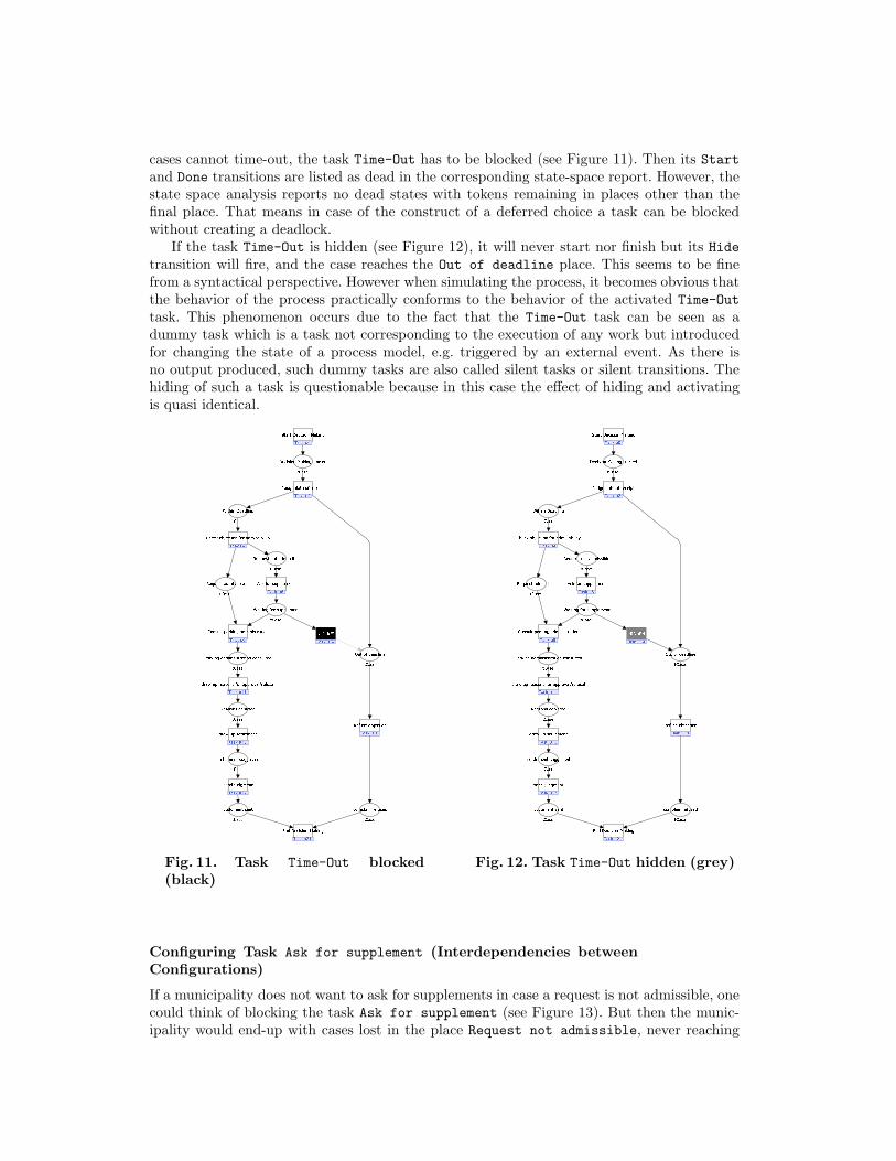
cases cannot time-out, the task Time-Out has to be blocked (see Figure 11). Then its Startand Done transitions are listed as dead in the corresponding state-space report. However, thestate space analysis reports no dead states with tokens remaining in places other than thefinal place. That means in case of the construct of a deferred choice a task can be blockedwithout creating a deadlock.

If the task Time-Out is hidden (see Figure 12), it will never start nor finish but its Hidetransition will fire, and the case reaches the Out of deadline place. This seems to be finefrom a syntactical perspective. However when simulating the process, it becomes obvious thatthe behavior of the process practically conforms to the behavior of the activated Time-Outtask. This phenomenon occurs due to the fact that the Time-Out task can be seen as adummy task which is a task not corresponding to the execution of any work but introducedfor changing the state of a process model, e.g. triggered by an external event. As there isno output produced, such dummy tasks are also called silent tasks or silent transitions. Thehiding of such a task is questionable because in this case the effect of hiding and activatingis quasi identical.

��

��

�� "!$#�%

��'&

#'��()%�� *�+$�� ,

��- �

.$� ��/ �0%�� 1+$�� ,

��2

34��(�,��(�� 5/ �� 6��

��-

7�� /��6�6�8 ��9:��

��;

(�/ ��<=��6:/ ��>� �/?��6�6�/ �@��8 A4/ �� 8

��

(�/ ��<B��6:�� 8 8 ��9:��

��C

�5D�� :� �/��(�9:� �� 8 � � E

��&

�5��8 �F6��/ �� ,:��(�9� �� / ��

��G

��(: ��(�,�9:��

��H

��F��5(��(�8 � ��

� �5��

��9:6�8 �� :/ �� (

� �5��

%�� )+$��I� ��,:�� / � ��(

� �$��

��J��K��F��F��(�9� �� 8 �

� �$��

LM�� ,:� �/?��K6�6�8 ��9:��

� �$��

�� 8 ��9:��F��,�,�� (

� �5��

LM� � D�� 1%��(�8 � ��

� �5��

3 ��(�,�9��K�F��

� �5��

N ��/ �� ,:��(�9:� �K�� / �� M��8 � ��(

� �5��

��J��F��(�9:� �� 8 �

� �$��

��>(��6�� (

� �5��

��H

��G

��&

��C

��

��;

��-

��2

��- �

��'&

��

Fig. 11. Task Time-Out blocked(black)

��

��

�� ! �� "��

��

#$��%��!��& � ��

� '!� ��

(�)*"�& �� * ��

� '!� ��

�� (� ��+� ��* ��

� '��

� '�� (�

� '�� (�

� '!� ��

� '!� ��

� ��)��,�% ��

� '!� ��

� '!� ��

� '��

� '!� ��

��

��

-.� � /�� 0��& � ��

'!/��1�2 �� *� � $��)*� ( �� 1�� & � � 3

�� 4�� 4

56+�7�7�,8

�� $��4�� $��4

-.�� *� �� 7 ��,"�"�& �)*��

��*2 ��)*��

�� (��$�:9�� (��$�:9

�� & �)*��% �� (� ��

�� ;<��"* �� & & �)*��

�� (��$�:=�� (��$�:=

>(�� ?��"��

�� ;@��"* �� ?� �� 7��"�"� ��A�& B� �� &

�� (��$�� (��$��

C �� *��)*� �, �� .�� & � ��

'!�� (��& �%"�� *��)��

�� D�� D

>E�F��,� ��%��%��)�� 1�& �

GH (�� $ ��"�"�& �)*��

�� I�� I

>E�F�� %��)*� � �� 1�& �

J�� K�� 0��

�� L�� L

>E�� 1�2 �(� � ��

�� (��$�:M�� (��$�:M

Fig. 12. Task Time-Out hidden (grey)

Configuring Task Ask for supplement (Interdependencies betweenConfigurations)

If a municipality does not want to ask for supplements in case a request is not admissible, onecould think of blocking the task Ask for supplement (see Figure 13). But then the munic-ipality would end-up with cases lost in the place Request not admissible, never reaching

the final task. So, the other option is to hide the task Ask for supplement which resultsin another issue: Non-admissible requests might time-out while waiting for an action by themunicipality. Formally this is not a problem, but content-wise it could be unintended behav-ior. To resolve this issue and create a valid configuration, the dummy task Time-Out must beblocked additionally whenever the task Ask for supplement is hidden (see Figure 14). Wecan conclude that configuration decisions are not always independent of each other.

��

��

��

��

! ��"$#�� %&�� '

��()�

*&� ��+ �,#�� -%&�� '

��.

/0��"�'��"�� 1+ �� 2��

��(

3&4 �)576&!�#

��8

"�+ ��9:��2;+ ��<� �+=��2�2�+ �>��? @0+ �� ?

��

"�+ ��9A��2;�� ? ? ��;��

��B

51C�� ;� �+��"��;� �� ? � � D

��

51��? �E2��+ �� ';��"�� + ��

��F

��"; ��"�'��;��

��G

��E��1"��"�? � ��

� 51��

��;2�? �� ;+ �� "

� 51��

#�� $%&��H� ��';�� + � ��"

� 5&��

��I��E��E��"�� ? �

� 5&��

JK�� ';� �+=��2�2�? ��;��

� 5&��

�� ? ��;��E��'�'�� "

� 51��

JK� � C�� -#��"�? � ��

� 51��

/ ��"�'��E��

� 51��

L ��+ �� ';��"��;� �� + �� K��? � ��"

� 51��

��I��E��"��;� �� ? �

� 5&��

��<"��2�� "

� 51��

��G

��F

��

��B

��

��8

��(

��.

��()�

��

��

Fig. 13. Task Ask for supplementblocked (black): Lost tokens mayremain in the place Request notadmissible

��

��

�� "!$#�%

��'&

#'��()%�� *�+$�� ,

��- �

.$� ��/ �0%�� 1+$�� ,

��2

34��(�,��(�� 5/ �� 6��

��-

7�89%:%:#�;

��<

(�/ ��=>��6?/ ��@� �/:��6�6�/ �A��B C4/ �� B

��

(�/ ��=D��6?�� B B ��E?��

��F

�5G�� ?� �/��(�E?� �� B � � H

��&

�5��B �I6��/ �� ,?��(�E� �� / ��

��J

��(? ��(�,�E?��

��K

��I��5(��(�B � ��

� �5��

��E?6�B �� ?/ �� (

� �5��

%�� )+$��9� ��,?�� / � ��(

� �$��

��L��M��I��I��(�E� �� B �

� �$��

NO�� ,?� �/:��M6�6�B ��E?��

� �$��

�� B ��E?��I��,�,�� (

� �5��

NO� � G�� 1%��(�B � ��

� �5��

3 ��(�,�E��M�I��

� �5��

P ��/ �� ,?��(�E?� �M�� / �� O��B � ��(

� �5��

��L��I��(�E?� �� B �

� �$��

��@(��6�� (

� �5��

��K

��J

��&

��F

��

��<

��-

��2

��- �

��'&

��

Fig. 14. To avoid asking for sup-plements, not only the Task Askfor supplement is hidden (grey), butalso task Time-Out must be blocked(black)

Configuring Task Judge date of receipt (Explicit Choice)

When executing the task Judge date of receipt an explicit choice how the process willcontinue is made: When the complain was received within the deadline, it will be checkedfor its admissibility, whereas in case it arrives too late, it will be refused. But maybe somemunicipalities want to be less restrictive with the initial deadlines and consider all objectionsas being received within the deadline. So all objections must be checked for their admissibility.However, neither hiding nor blocking of the task Judge date of receipt helps here. If it isblocked the process will never go beyond this task. If it is hidden, tokens can still be placedinto the Out of deadline place.

In the previous scenario we could achieve the desired behavior by hiding one (Ask forsupplement) and blocking another task (Time-Out). But also this approach is impossible to

apply as neither hiding nor blocking of task Refuse objection can prevent that tokens areput into the place Out of deadline and as soon as a token is in this place it cannot bechecked for its admissibility anymore.

The only chance of enforcing the desired behavior is, to go to a lower level, i.e., to have alook at the implementation of the choice on the task page. In a standard Petri net an explicitchoice can only be modelled by a deferred choice with subsequent silent transitions. In ourimplementation of the XOR-split, these silent transitions are the multiple Done transitions.Only when explicitly blocking the particular Done transition on this task-level (see Figure 15),it is possible to restrict the process model to the desired behavior6. So within a sound processmodel the outcome of an explicit choice cannot be restricted, i.e., configured, at the processlevel, but on lower implementation levels.

��

��

��

��

��

��

� � �� !"�� $#� � !��# %& ��'"( � �� !"��%

��

) (�* �+",.- ��/�0�1 ��2 �43�5 )

�� /�0 ,

6 & ��'7( � �� !�

*�8 /9��# %�:( /�� 8 /9�;# ��'7( � �� !"��%�:�� (�* # '7( � �� !"��/��#�% %�:

</�� +,=-�/��

�/�� +?></��

@ * � +,@ * � � ��

A �� ( /�� A �� ( /�� B�� A �� ( /��

��/��C� � � ( ��D � ��

A �� ( /��

@ *

</��/��

Fig. 15. Done transition blocked (black) in the sub-page of the Judge date ofreceipt task: The task can only exit via the left path.

This concludes our analysis of four configuration scenarios. Using the four scenarios it hasbeen shown that the state space analysis and the simulation facilities of CPN Tools can beused to evaluate configuration decisions.

4 Conclusions

By analyzing a set of reference models designed using the business process modelling languageof Protos, we discovered that these models do not conform to well defined soundness criteriawhich also prevents the meaningful use of Protos’ simulation features. The main reasons forthis are that the developers of the models either see no value in the Protos simulation, or theyare not aware of its value. We also realized that it is unclear which of the parameters thatcan be specified in Protos are actually used in the Protos simulation. To improve the valueof simulation in this context, we developed the Protos2CPN transformation which allows thesimulation of Protos models in CPN Tools. The simulation of Protos models in CPN Tools6 The configuration of Done transitions is not yet implemented in the Protos2C-CPN transformation.

makes the running process visible by depicting the moving cases as tokens within the processmodel. It therefore allows for a detailed inspection of the running process. In addition, themonitoring features of CPN Tools enable the generation of complex statistics. The modelscreated by our Protos2CPN transformation already include some basic measurements whichcan be extended by experienced users.

In a second step we developed Protos2C-CPN. As far as we know, this is the first im-plemented tool offering explicit support for reference model adaptation by adding standardconfiguration features to the tasks in the reference models. These features permit the restric-tion of the possible behavior of the reference model directly in the model without changing itsnet structure. The simulation features of CPN Tools allow for performance testing and com-parison of different process configurations. By making use of CPN Tools’ state space analysisfeature, we were able to test configurations on their admissibility in sound process models,but also realized that certain configurations are undesirable in specific contexts.

However, it might be possible to resolve such problems on lower model levels. To do thiswe plan to explore configuration in the context of the workflow patterns [6]. We assume thatby analyzing all workflow patterns on their configurability aspect, it might be possible todevelop configuration patterns which depict how configuration can be implemented in thecontext of the particular workflow pattern. If such patterns are available, we could developan improved version of Protos2C-CPN which might even be able to transform the configuredmodel back into an ordinary process model without configuration features.

Acknowledgements

The authors would like to thank Kurt Jensen and Lisa Wells for their continuous feedbackand support related to the use of CPN Tools, as well as Pallas Athena for providing the Protosreference models.

References

1. W.M.P. van der Aalst. Verification of Workflow Nets. In P. Azema and G. Balbo, editors,Application and Theory of Petri Nets 1997, volume 1248 of Lecture Notes in Computer Science,pages 407–426. Springer-Verlag, Berlin, 1997.

2. W.M.P. van der Aalst. Business Process Management Demystified: A Tutorial on Models, Sys-tems and Standards for Workflow Management. In J. Desel, W. Reisig, and G. Rozenberg,editors, Lectures on Concurrency and Petri Nets, volume 3098 of Lecture Notes in ComputerScience, pages 1–65. Springer-Verlag, Berlin, 2004.

3. W.M.P. van der Aalst and T. Basten. Inheritance of workflows: an approach to tackling problemsrelated to change. Theoretical Computer Science, 270(1-2):125–203, January 2002.

4. W.M.P. van der Aalst, P.J.N. de Crom, R.R.H.M.J. Goverde, K.M. van Hee, W.J. Hofman, H.A.Reijers, and R.A. van der Toorn. ExSpect 6.4 An Executable Specification Tool for HierarchicalColored Petri Nets. In M. Nielsen and D. Simpson, editors, Application and Theory of Petri Nets2000: 21st International Conference, ICATPN 2000, volume 1825 of Lecture Notes in ComputerScience, pages 455–464, Berlin, Germany, January 2000. Springer.

5. W.M.P. van der Aalst, A. Dreiling, F. Gottschalk, M. Rosemann, and M.H. Jansen-Vullers.Configurable Process Models as a Basis for Reference Modeling. In C. Bussler and A. Haller,editors, Business Process Management Workshops: BPM 2005 International Workshops, BPI,BPD, ENEI, BPRM, WSCOBPM, BPS. Revised Selected Papers, volume 3812 of Lecture Notesin Computer Science, pages 512–518, Berlin Heidelberg, 2006. Springer Verlag.

6. W.M.P. van der Aalst, A.H.M. ter Hofstede, B. Kiepuszewski, and A.P. Barros. Workflow Pat-terns. Distributed and Parallel Databases, 14(1):5–51, 2003.

7. T. Basten and W.M.P. van der Aalst. Inheritance of behavior. Journal of Logic and AlgebraicProgramming, 47(2):47–145, 2001.

8. J. Becker, P. Delfmann, A. Dreiling, R. Knackstedt, and D. Kuropka. Configurative ProcessModeling – Outlining an Approach to increased Business Process Model Usability. In Proceed-ings of the 15th Information Resources Management Association International Conference, NewOrleans, 2004. Gabler.

9. J. Becker, P. Delfmann, and R. Knackstedt. Konstruktion von Referenzmodellierungssprachen:Ein Ordnungsrahmen zur Spezifikation von Adaptionsmechanismen fur Informationsmodelle (inGerman). Wirtschaftsinformatik, 46(4):251–264, 2004.

10. J. vom Brocke and C. Buddendick. Konstruktionstechniken fur die Referenzmodellierung (inGerman). In J. Becker and P. Delfmann, editors, Referenzmodellierung. Grundlagen, Technikenund domanenbezogene Anwendung, also Proceedings of the 8th Fachtagung Referenzmodellierung,pages 19–48, Heidelberg, 2004.

11. Thomas Curran, Gerhard Keller, and Andrew Ladd. SAP R/3 Business Blueprint: understandingthe business process reference model. Prentice Hall PTR, Upper Saddle River, New Jersey, 1998.

12. Deloitte & Touche Bakkenist. ExSpect Home Page. http://www.exspect.com.13. F. Gottschalk, W.M.P. van der Aalst, and M.H. Jansen-Vullers. Configurable Process Models –

A Foundational Approach. In Referenzmodellierung 2006, Passau, Germany, 2006. to appear inLecture Notes in Computer Science.

14. K. Jensen. Coloured Petri Nets. Basic Concepts, Analysis Methods and Practical Use. Volume1. EATCS monographs on Theoretical Computer Science. Springer-Verlag, Berlin, 1997.

15. R.J. Paul, G.M. Giaglis, and V. Hlupic. Simulation of business processes. The American Behav-ioral Scientist, 42(10):1551–1576, August 1999.

16. M. Rosemann and W.M.P. van der Aalst. A Configurable Reference Modelling Language. Infor-mation Systems, 2005. (to appear, also available via BPMCenter.org).

17. K. Sarshar and P. Loos. Comparing the Control-Flow of EPC and Petri Net from the End-User Perspective. In W.M.P. van der Aalst, B. Benatallah, F. Casati, and F. Curbera, editors,Proceedings of the 3rd International Conference on Business Process Managemen (BPM 2005),volume 3649 of Lecture Notes in Computer Science, pages 434–439, Nancy, France, September2005. Springer-Verlag.

18. R. Schutte. Grundsatze ordnungsmaßiger Referenzmodellierung – Konstruktion konfigurations-und anpassungsorientierter Modelle (in German). Gabler, Wiesbaden, 1998.

19. A. Schwegmann. Objektorientierte Referenzmodellierung: theoretische Grundlagen und praktischeAnwendung (in German). Gabler, Wiesbaden, 1999.

20. A. Sharp and P. McDermott. Workflow Modeling: Tools for Process Improvement and ApplicationDevelopment. Artech House Publishers, Norwood, MA, 2001.

21. H.M.W. Verbeek and W.M.P. van der Aalst. Woflan Home Page, Eindhoven University of Tech-nology, Eindhoven, The Netherlands. http://is.tm.tue.nl/research/woflan.

22. H.M.W. Verbeek and W.M.P. van der Aalst. Woflan 2.0: A Petri-net-based Workflow DiagnosisTool. In M. Nielsen and D. Simpson, editors, Application and Theory of Petri Nets 2000, volume1825 of Lecture Notes in Computer Science, pages 475–484. Springer-Verlag, Berlin, 2000.

23. H.M.W. Verbeek, T. Basten, and W.M.P. van der Aalst. Diagnosing Workflow Processes usingWoflan. The Computer Journal, 44(4):246–279, 2001.

24. H.M.W. Verbeek, M. van Hattem, H.A. Reijers, and W. de Munk. Protos 7.0: Simulation MadeAccessible. In G. Ciardo and P. Darondeau, editors, Applications and Theory of Petri Nets2005: 26th International Conference (ICATPN 2005), volume 3536 of Lecture Notes in ComputerScience, pages 465–474, Miami, USA, June 2005. Springer-Verlag.

25. A. Vinter Ratzer, L. Wells, H. M. Lassen, M. Laursen, J. F. Qvortrup, M. S. Stissing, M. West-ergaard, S. Christensen, and K. Jensen. CPN Tools for Editing, Simulating, and AnalysingColoured Petri Nets. In W.M.P. van der Aalst and E. Best, editors, Applications and Theory ofPetri Nets 2003: 24th International Conference, ICATPN 2003, volume 2679 of Lecture Notes inComputer Science, pages 450–462. Springer Verlag, January 2003.

26. L. Wells. Monitoring a CP-net. http://wiki.daimi.au.dk/cpntools-help/monitoring a cp-net.wiki.

http://is.tm.tue.nl/staff/wvdaalst/BPMcenter/reports/2003/BPM-03-08.pdf�

Sweep-line Analysis of DCCP Connection Management

Somsak Vanit-Anunchai, Jonathan Billington and Guy Edward Gallasch

Computer Systems Engineering CentreUniversity of South Australia, Mawson Lakes Campus, SA 5095, AUSTRALIA

Email: [email protected], {jonathan.billington|guy.gallasch}@unisa.edu.au

Abstract. State space explosion is a key problem in the analysis of finite state systems. Thesweep-line method is a state exploration method which uses a notion of progress to allow statesto be deleted from memory when they are no longer required. This reduces the peak numberof states that need to be stored, while still exploring the full state space. The technique showspromise but has never achieved reductions greater than about a factor of 10 in the numberof states stored in memory for industrially relevant examples. This paper discusses sweep-lineanalysis of the connection management procedures of a new Internet standard, the DatagramCongestion Control Protocol (DCCP). As the intuitive approaches to sweep-line analysis arenot effective, we introduce new variables to track progress. This creates further state explosion.However, when used with the sweep-line, the peak number of states is reduced by over twoorders of magnitude compared with the original. Importantly, this allows DCCP to be analysedfor larger parameter values.

Keywords: State Space Methods, Sweep-line, DCCP, Coloured Petri Nets, State Explosion.

1 Introduction

The state space method is one of the main approaches for formally analysing and verify-ing the behaviour of concurrent and distributed systems. In essence, this method generatesall or part of the reachable states of the system. After the state space is generated, manyanalysis and verification questions about the system’s behaviour (such as ”does the systemdeadlock and livelock?”), can be answered. Unlike theorem proving, state space analysis toolsare easier to use because they involve less complex mathematics that is often hidden byautomatic computer tools, and they can provide counter examples for debugging purposes.Despite these advantages, the state space approach suffers from the well known state explosionproblem [23]. Even relatively small systems can generate state spaces that cannot be storedin computer memory. Thus many attempts have been made to alleviate this problem. Anexcellent overview and literature review about the state explosion problem is given in [23].The attempts to alleviate state explosion fall into three broad classes. The first considersmethods that represent the state space in a condensed or compact form, such as symmetryreduction [4,13]. The second class restricts state space exploration to a subset of the reachablestates and includes partial order methods [21, 26] such as stubborn sets [22]. The third classinvolves deleting or throwing away states or state information on-the-fly during state spaceexploration. It includes methods such as bit-state hashing [11,27], state space caching [8,10],the sweep-line method [2,15] and the pseudo-root technique [20]. To further reduce the statespace, techniques from the different classes have also been combined, e.g. sweep-line andequivalence [1].

The sweep-line method exploits a notion of progress exhibited in the system being anal-ysed. Progress mappings are defined by the user, to map the states of the system into a setof ordered progress values. Based on progress values, this method deletes old states frommemory by reasoning that states with a lower progress value will not (or are unlikely to) be

reached from states with a higher progress value. During exploration, a number of systemproperties, such as absence of deadlocks, can be verified on-the-fly.

In the area of formal analysis and verification of computer protocols that recover from lossusing retransmissions, the maximum number of retransmissions of messages plays an impor-tant role in state explosion. When the maximum number of retransmissions increases, the sizeof the state space tends to explode rapidly. When using a small maximum number of retrans-missions, errors tend to reveal themselves quickly, but this does not guarantee that the systemis error free for larger values of the maximum number of retransmissions. Thus it is necessaryto extend state space analysis to include the highest maximum number of retransmissionspossible, up to the limit specified by the protocol’s specification. Previously we have usedthe sweep-line method to verify termination properties of Coloured Petri Net (CPN) [12,17]models of various protocols such as the Wireless Transaction Protocol (WTP) [9], the InternetOpen Trading Protocol (IOTP) [6], and the Transmission Control Protocol [5].

The Datagram Congestion Control Protocol (DCCP), specified in Request For Comments(RFC) 4340 [14], is a new transport protocol proposed by the Internet Engineering Task Force(IETF). The protocol is designed to support various kinds of congestion control mechanismsused by different delay sensitive applications. We use CPNs to build and analyse a formalexecutable model of DCCP’s connection management procedures according to RFC 4340 [14].Our analysis shows that DCCP connection establishment can fail when sequence numberswrap1. However, state explosion limits our analysis to a maximum of only one retransmission.We need to extend the analysis to cover two retransmissions and to determine two properties:whether the undesired deadlocks are still present; and whether any new errors have emergedas a result of the additional retransmissions.

Instead of applying the more conventional approach of trying to reduce the size of thestate space, we induce state space explosion by introducing new state variables into thespecification model in order to capture additional information during model execution. Bycarefully selecting new state variables, the state space of the augmented model has a structurewhich facilitates far more efficient sweep-line analysis when compared to the state space ofthe specification model.

The contribution of this paper is two fold. Firstly, this paper provides some insight intohow an effective progress mapping for the DCCP connection management model is derived.An effective progress mapping is key to the performance of the sweep-line. Secondly, we applysweep-line analysis to the augmented model. This method can significantly reduce the numberof peak states stored compared with the sweep-line analysis of the specification model. Thuswe can extend the analysis of DCCP connection establishment to scenarios which could notbe reached with conventional analysis.

This paper is organised as follows. Section 2 briefly describes the DCCP connection man-agement CPN model. Section 3 identifies sources of progress and derives a progress mappingfor DCCP connection management. The sweep-line analysis results obtained for scenarioswhere sequence numbers wrap are discussed in Section 4. Section 5 presents conclusions andfuture work. We assume some familiarity with CPNs [12,17].

1 Sequence number wrap occurs when the sequence number rolls over the maximum sequence number to zero.

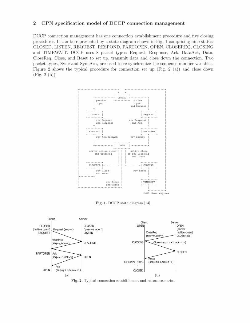
2 CPN specification model of DCCP connection management

DCCP connection management has one connection establishment procedure and five closingprocedures. It can be represented by a state diagram shown in Fig. 1 comprising nine states:CLOSED, LISTEN, REQUEST, RESPOND, PARTOPEN, OPEN, CLOSEREQ, CLOSINGand TIMEWAIT. DCCP uses 8 packet types: Request, Response, Ack, DataAck, Data,CloseReq, Close, and Reset to set up, transmit data and close down the connection. Twopacket types, Sync and SyncAck, are used to re-synchronize the sequence number variables.Figure 2 shows the typical procedure for connection set up (Fig. 2 (a)) and close down(Fig. 2 (b)).

+---------------------------+ +---------------------------+| v v || +----------+ || +-------------+ CLOSED +------------+ || | passive +----------+ active | || | open open | || | snd Request | || v v || +----------+ +----------+ || | LISTEN | | REQUEST | || +----+-----+ +----+-----+ || | rcv Request rcv Response | || | snd Response snd Ack | || v v || +----------+ +----------+ || | RESPOND | | PARTOPEN | || +----+-----+ +----+-----+ || | rcv Ack/DataAck rcv packet | || | | || | +----------+ | || +------------>| OPEN |<-----------+ || +--+-+--+--+ || server active close | | | active close || snd CloseReq | | | or rcv CloseReq || | | | snd Close || | | | || +----------+ | | | +----------+ || | CLOSEREQ |<---------+ | +--------->| CLOSING | || +----+-----+ | +----+-----+ || | rcv Close | rcv Reset | || | snd Reset | | ||<---------+ | v || | +----+-----+ || rcv Close | | TIMEWAIT | || snd Reset | +----+-----+ |+-----------------------------+ | |

+-----------+2MSL timer expires

Fig. 1. DCCP state diagram [14].

Client Server

CLOSED CLOSED [active open] Request (seq=x) [passive open] REQUEST LISTEN

Response (seq=y,ack=x) RESPOND

PARTOPEN Ack

(seq=x+1,ack=y) OPEN

Ack

OPEN (seq=y+1,ack=x+1)

(a)

Client Server OPEN OPEN

[server CloseReq active close]

(seq=m,ack=n) CLOSEREQ

CLOSING Close (seq = n+1, ack = m)

CLOSED

Reset TIMEWAIT(2 MPL) (seq=m+1,ack=n+1) . .

CLOSED

(b)

Fig. 2. Typical connection establishment and release scenarios.

In brief, a connection is initiated by an application at the client issuing an “active open”command. (We assume that the application at the server has issued a “passive open” com-mand.) After receiving the “active open” the client sends a DCCP-Request packet to theserver to initialise sequence numbers, and enters the REQUEST state. The server replieswith a DCCP-Response packet, indicating that it is willing to communicate with the clientand acknowledging the DCCP-Request. The client sends a DCCP-Ack (or DCCP-DataAck)packet to acknowledge the DCCP-Response packet and enters the PARTOPEN state. Theserver acknowledges the receipt of the DCCP-Ack, enters the OPEN state and is ready for datatransfer. Upon receipt of a DCCP-Ack (or DCCP-Data, DCCP-DataAck or DCCP-SyncAck)packet, the client also enters OPEN and is now also ready for data transfer.

For connection close down, the application at the server issues a “server active close”command. The server sends a DCCP-CloseReq and enters the CLOSEREQ state. The client,upon receiving the DCCP-CloseReq, enters CLOSING and generates a DCCP-Close packetin response. After the server receives the DCCP-Close packet, it responds with a DCCP-Resetpacket and enters the CLOSED state. When the client receives the DCCP-Reset packet, itholds the TIMEWAIT state for 2 maximum packet lifetimes before also entering the CLOSEDstate.

Alternatively, either side may send a DCCP-Close packet to close the connection whenreceiving an “active close” command from the application. The end that sends the DCCP-Close packet will hold the TIMEWAIT state as shown in Fig. 3. Beside these three closingprocedures, there are another 2 possible scenarios concerned with simultaneous closing. Thefirst procedure is invoked when both users issue an “active close”. The second occurs whenthe client user issues an “active close” and the application at the server issues the “serveractive close” command. For a detailed description of the connection set up and close downprocedures, see [14].


[active close] Close CLOSING (seq= m, ack= n)

CLOSED

Reset

TIMEWAIT(2 MPL) (seq= n+1, ack= m) .

.

CLOSED

(a)


Close [active close] (seq= m,ack= n) CLOSING

CLOSED

Reset

(seq= n+1, ack= m) TIMEWAIT(2 MPL)

. .

CLOSED

(b)

Fig. 3. Alternative close down procedures.

During the connection, DCCP entities maintain a set of variables. In addition to the stateand timers, the important variables are Greatest Sequence Number Sent (GSS), GreatestSequence Number Received (GSR), Greatest Acknowledgement Number Received (GAR),Initial Sequence Number Sent and Received (ISS and ISR), Valid Sequence Number windowwidth (W) and Acknowledgement Number validity window width (AW). Based on the statevariables, the valid sequence and acknowledgement number intervals are defined by Sequence

Number Window Low and High [SWL,SWH], and Acknowledgement Number Window Lowand High [AWL,AWH].

We use Design/CPN [19] to build and maintain our DCCP connection management CPNmodels. In this paper we are restricted to describing details of the model at a high level only.More details can be found in [25].

2.1 Modelling assumptions

Our model represents a detailed DCCP connection management specification of RFC 4340.We consider a single connection instance while ignoring the procedures for data transfer,congestion control and other feature options. A DCCP packet is modelled by its packettype, and long (or short) sequence and acknowledgement numbers. Other fields in the DCCPheader are omitted because they do not affect the operation of the connection managementprocedure. Malicious attacks are not considered. In this paper we only discuss the case whenthe communication channels can delay and reorder packets without loss.

2.2 Model structure and the top level page

The DCCP Connection management (DCCP-CM) CPN model comprises four hierarchicallevels shown in Fig. 4. It has a total of 6 places, 53 executable transitions, 15 substitutiontransitions and 18 ML functions. The top level page named DCCP#3 is the DCCP overviewpage shown in Fig. 5. Two substitution transitions DCCP C and DCCP S in Fig. 5 representthe client and the server. Both are linked to the second level page named DCCP CM. Theclient and server communicate via two channel places, shown in the middle of Fig. 5. Theplaces Ch C S and Ch S C each model a unidirectional reordering channel, from the client tothe server and the server to the client respectively.

2.3 Global declarations

The global declarations define data structures, colour sets and any associated variables usedin the model. The declarations are written in CPN ML [3], a variant of Standard ML [18].An example of the Declarations is given in Fig 6. Figure 6 declares PACKETS (line 21-24), the colour set of the channel places, as a union of four colour sets: Type1LongPkt,Type2LongPkt, Type1ShortPkt, and Type2ShortPkt. Long sequence numbers (SN48) in line11 are represented using the infinite integer type and range from zero to 248 − 1. Shortsequence numbers (SN24) in line 13 are represented by integers ranging from zero to 224 − 1.Each packet (lines 17-20) is defined by a product comprising the Packet Type (lines 2-5), X(Extended Sequence Number bit, called ‘X’ in [14], line 8) and the sequence number (or arecord of sequence and acknowledgement numbers). Short sequence numbers are allowed onlyfor DCCP-Data, DCCP-Ack and DCCP-DataAck packets. Thus line 4 defines a packet typefor DCCP-Data with short sequence numbers, while line 5 defines a different packet typefor DCCP-Ack and DCCP-DataAck because they also include acknowledgements. Strongtyping of packets is very useful for developing and debugging the model. Strong typing allowsautomatic detection of violations of the typing rules via a syntax check.

The places Client State and Server State in Fig. 5, typed by CB (Control Block), storeDCCP state information for the client and server entities respectively. We classify DCCPstates into three groups according to their functional behaviour: idle, request and active

DCCP#3 M Prime

DCCP_CM#4

RcvSync#13

Declarations#2

PartOpen#9

ClosingDown#11

DataTransfer#10

RcvReset#14

Retransmission#15

Request#7

UnExpected#16

IdleState#6

UserCommand#5

Respond#8

CommonProcessing#12

Hierarchy#1

RcvInvalid#17

DCCP_SDCCP_C

UserCMD

ClosingDown

Idle_State

Common

RcvSync

RcvReset

UnexpectedPkt

RcvInvalidHeader

Request

Respond

PartOpen

TimeOut

DataTransfer

Fig. 4. The DCCP hierarchy page.

states. The differences are mainly related to how an entity responds to DCCP-Reset andDCCP-Sync packets. When in the CLOSED, LISTEN and TIMEWAIT states, the GSS,GSR, GAR, ISS and ISR state variables do not exist, while the client in the REQUEST statehas only GSS and ISS instantiated. Thus we define each group with a different set of statevariables. Figure 7 defines CB (line 13-15) as a union of colour sets: IDLE, REQUEST andACTIVExRCNTxGSxISN.

IDLE (line 7 of Fig 7) defines three idle states: CLOSED, LISTEN and TIMEWAIT. TheCLOSED state is split into CLOSED I to represent the initial CLOSED state and CLOSED Fto represent a terminal CLOSED state. Differentiating the initial CLOSED state and the finalCLOSED state helps increase the effectiveness of the sweep-line method when using the clientand server states as a measure of progress. Because we consider only one connection instance,splitting the CLOSED state into CLOSED I and CLOSED F does not affect the protocol’sbehaviour. The colour set REQUEST (line 8) is a product comprising RCNT (RetransmissionCounter, line 2), GSS and ISS. Because there is only one state in this group, the REQUESTstate is already distinguished from other states by using the ML constructor, ReqState, in theunion defined in line 14. ACTIVE (line 9) defines five DCCP states: RESPOND, PARTOPEN,OPEN, CLOSEREQ and CLOSING. Because the client and server respond to the CloseReqpacket differently in the OPEN and CLOSING states, we differentiate these states for theclient and server: C OPEN and C CLOSING for the client; and S OPEN and S CLOSINGfor the server. ACTIVExRCNTxGSxISN (line 10) is a product comprising ACTIVE (line9), RCNT, GS (Greatest Sequence and Acknowledgement Numbers, line 3) and ISN (Initial

CB

Client_State

1‘IdleState CLOSED_I

COMMAND

App_Client

1‘a_Open

DCCP_SHS

DCCP_CM#4Ch_S_C->Ch_A_BCh_C_S->Ch_B_AServer_State->StateApp_Server->App

Ch_C_S

PACKETS

Ch_S_C

PACKETS

DCCP_CHS

DCCP_CM#4Ch_C_S->Ch_A_BCh_S_C->Ch_B_AClient_State->StateApp_Client->App

CB

Server_State

1‘IdleState CLOSED_I

COMMAND

App_Server

1‘p_Open

Fig. 5. The DCCP overview page.

1: (* Packet Types *)

2: color PktType1 = with Request | Data;

3: color PktType2 = with Sync | SyncAck | Response | Ack | DataAck | CloseReq | Close | Rst;

4: color DATA = subset PktType1 with [Data];

5: color ACK_DATAACK = subset PktType2 with [DataAck,Ack];

6:7: (* Extended Sequence Number Bit*)

8: color X = bool;

9:10: (* Sequence and Acknowledgement Number (Long/Short) *)

11: color SN48 = IntInf with ZERO..MaxSeqNo48;

12: color SN48_AN48 = record SEQ:SN48*ACK:SN48;

13: color SN24 = int with 0..max_seq_no24;

14: color SN24_AN24 = record SEQ:SN24*ACK:SN24;

15:16: (* Four Kinds of Packet *)

17: color Type1LongPkt=product PktType1*X*SN48;

18: color Type2LongPkt=product PktType2*X*SN48_AN48;

19: color Type1ShortPkt=product DATA*X*SN24;

20: color Type2ShortPkt=product ACK_DATAACK*X*SN24_AN24;

21: color PACKETS = union PKT1:Type1LongPkt

22: + PKT2:Type2LongPkt

23: + PKT1s:Type1ShortPkt

24: + PKT2s:Type2ShortPkt;

Fig. 6. Definition of DCCP PACKETS.

Sequence Numbers, line 4). Places Client State and Server State (Fig. 5) both have an initialmarking of one CLOSED I idle state token.

Figure 7 also defines a colour set COMMAND on line 17. The places App Client andApp Server in Fig 5, typed by COMMAND, model DCCP user commands (i.e. commandsthat can be issued by the applications that use DCCP). For example, the user command1‘a Open is the initial marking of App Client indicating that the client’s application desiresto open a connection.

1: (* DCCP variables: Counter; Greatest Sequence Numbers; Initial Sequence Numbers *)

2: color RCNT = int; (* Retransmission Counter *)

3: color GS = record GSS:SN48*GSR:SN48*GAR:SN48;

4: color ISN = record ISS:SN48*ISR:SN48;

5:6: (* Major States *)

7: color IDLE = with CLOSED_I | LISTEN | TIMEWAIT | CLOSED_F;

8: color REQUEST = product RCNT*SN48*SN48;

9: color ACTIVE = with RESPOND | PARTOPEN | S_OPEN | C_OPEN | CLOSEREQ | C_CLOSING |S_CLOSING;

10: color ACTIVExRCNTxGSxISN = product ACTIVE*RCNT*GS*ISN;

11:12: (* DCCP’s Control Block *)

13: color CB = union IdleState:IDLE

14: + ReqState:REQUEST

15: + ActiveState:ACTIVExRCNTxGSxISN;

16: (* Application Commands *)

17: color COMMAND = with p_Open | a_Open | a_Close | server_a_Close;

Fig. 7. DCCP’s control block and commands.

3 Sweep-line analysis

The success of applying sweep-line relies on the notion of a progress measure which is de-fined [2] as a tuple P = (O,�, ϕ), where O is a set of progress values, � ⊆ O×O is a partialordering operator on the progress values, and ϕ : M → O is a progress mapping functionfrom markings of the CPN model, M, to progress values. Gordon et al. [9] point out thatthe protocol can exhibit more than one source of progress and suggests the use of a vectorof progress values that we shall call a progress vector. In [5] the progress vector is used inconjunction with lexicographical ordering. We use this approach to analyze the DCCP-CMCPN model.

The sweep-line algorithm generates the successors of all unexplored states with the lowestprogress value first. Once all states with this lowest progress value have been explored, theywill be deleted from memory and the conceptual “sweep-line” will move on to states with thenew lowest progress value. A progress mapping is said to be monotonic if, for every reachablestate, it has a progress value equal to or less than all of its successors. When this is not thecase, i.e. at least one successor of one state has a progress value that is less than its predecessor(representing regress rather than progress), the sweep-line must conduct additional sweeps of(part of) the state space, using the destinations of these so-called regress edges as roots of anew sweep. Thus, some parts in the state space may be explored more than once. However,the sweep-line still guarantees full exploration of a state space and is guaranteed to terminate.Detailed explanations of the sweep-line method can be found in [2, 15].

3.1 Notation

We define some notation used for identifying sources of progress in a CPN model. Let M ∈ M

be a marking of the CPN model. M(p) is the marking of place p (the multiset of tokenson place p) and ‖M(p)‖ is the number of tokens on place p. Measures of progress, such asthe greatest sequence number sent, are often encapsulated in a product token residing ona state place, e.g. Client State. To extract information from a product token we shall useprojection functions. Our progress mappings operate on markings, which are multisets oftokens rather than tokens themselves. However, when p is a state place, it only contains one

token (∀M ∈ [M0〉, ||M(p)|| = 1, where [M0〉 is the set of reachable markings), and henceM(p) is a singleton multiset. Therefore in this situation, if we wish to extract informationfrom the single token in such a place we firstly need to convert the marking of the place,which is a singleton multiset, into its basis element (i.e. the token). We define this conversionfunction (conv) as follows using standard set theory to represent a multiset (a function) bya set of pairs comprising a basis element (i.e. from its domain) and its multiplicity (from itsrange).

Definition 1. Let MS : B → N be a multiset over B and BMS1 be the set of all singletonmultisets over a basis set B: BMS1 = {{(b, 1)}| b ∈ B}. A function that converts a singletonmultiset to its basis element is given by conv : BMS1 → B, where conv({(b, 1)}) = b.

3.2 Usual sources of progress

The following describes three usual sources of progress.

1. Sequence Number Variables Firstly, consider GSS. Every time the client or serversends a packet, the state variable GSS (the Greatest Sequence number Sent) increases byone. GSS is stored within a single product token in the places Client State and Server State.However when an entity is in an idle state (CLOSED, LISTEN and TIMEWAIT), there is noGSS. To capture the progress of GSS from the marking of the place Client State we define aprogress mapping for the client ϕc

gss : M → N, where the superscript “c” refers to the Cliententity and

ϕcgss(M) = Projgss(conv(M(Client State))) (1)

and Projgss takes a state variable of type CB and returns GSS for active states and ISS oth-erwise. During connection establishment and close down, the number of transmitted packetsis small. We consider that the sequence number may wrap only once. If the GSS value is lessthan ISS, it means that the GSS value has wrapped. In this situation, Projgss returns GSSplus 248 in order to maintain increasing progress values. If there is no GSS value in the statevariable, Projgss returns ISS because it is the starting value of GSS for each connection. Theprogress mapping, ϕs

gss, ϕcgsr, ϕs

gsr, ϕcgar and ϕs

gar for other client and server sequence numbervariables can also be defined in a similar way.

2. Major States Both entities progress through the states defined by colour sets IDLE,REQUEST and ACTIVE. To capture this progress from the token in the place Client State,we define a progress mapping ϕc

state : M → N where

ϕcstate(M) = State2Num(Projstate(conv(M(Client State)))) (2)

The projection function, Projstate, takes a state variable of type CB and returns the DCCPstate. Function State2Num maps this state to an integer according to the ordering of DCCPstates shown in Column 1 of Table 1. The server’s progress mapping, ϕs

state, is defined analo-gously, using the ordering of DCCP states shown in Column 3 of Table 1.

Because of lost and delayed packets, an entity may retransmit. The progress exhibitedby the retransmission counters (RCNTs) has already been covered by GSS because GSS isincreased for every packet sent, including retransmissions. Thus the progress captured byRCNTs is not needed. However when retransmission occurs, the state is not changed, andhence, intuitively, it is useful to include both major state and GSS in progress mappings.

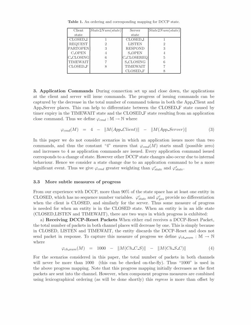
Table 1. An ordering and corresponding mapping for DCCP state.

Client State2Num(state) Server State2Num(state)state state

CLOSED I 1 CLOSED I 1REQUEST 2 LISTEN 2

PARTOPEN 3 RESPOND 3C OPEN 4 S OPEN 4

C CLOSING 6 C CLOSEREQ 5TIMEWAIT 7 S CLOSING 6CLOSED F 8 TIMEWAIT 7

CLOSED F 8

3. Application Commands During connection set up and close down, the applicationsat the client and server will issue commands. The progress of issuing commands can becaptured by the decrease in the total number of command tokens in both the App Client andApp Server places. This can help to differentiate between the CLOSED F state caused bytimer expiry in the TIMEWAIT state and the CLOSED F state resulting from an applicationclose command. Thus we define ϕcmd : M → N where

ϕcmd(M) = 4 − ‖M(App Client)‖ − ‖M(App Server)‖ (3)

In this paper we do not consider scenarios in which an application issues more than twocommands, and thus the constant “4” ensures that ϕcmd(M) starts small (possible zero)and increases to 4 as application commands are issued. Every application command issuedcorresponds to a change of state. However other DCCP state changes also occur due to internalbehaviour. Hence we consider a state change due to an application command to be a moresignificant event. Thus we give ϕcmd greater weighting than ϕc

state and ϕsstate.

3.3 More subtle measures of progress

From our experience with DCCP, more than 90% of the state space has at least one entity inCLOSED, which has no sequence number variables. ϕc

state and ϕcgss provide no differentiation

when the client is CLOSED, and similarly for the server. Thus some measure of progressis needed for when an entity is in the CLOSED state. When an entity is in an idle state(CLOSED,LISTEN and TIMEWAIT), there are two ways in which progress is exhibited:

a) Receiving DCCP-Reset Packets When either end receives a DCCP-Reset Packet,the total number of packets in both channel places will decrease by one. This is simply becausein CLOSED, LISTEN and TIMEWAIT, the entity discards the DCCP-Reset and does notsend packet in response. To capture this measure of progress we define ϕch num : M → N

whereϕch num(M) = 1000 − ‖M(Ch C S)‖ − ‖M(Ch S C)‖ (4)

For the scenarios considered in this paper, the total number of packets in both channelswill never be more than 1000 (this can be checked on-the-fly). Thus “1000” is used inthe above progress mapping. Note that this progress mapping initially decreases as the firstpackets are sent into the channel. However, when component progress measures are combinedusing lexicographical ordering (as will be done shortly) this regress is more than offset by

progress captured in other ‘more significant’ component progress measures when the numberof messages in the channel are increasing.

b) Receiving non-DCCP-Reset Packets When any packet but DCCP-Reset is re-ceived from one channel by an entity in an idle state, it will send a DCCP-Reset packet intothe other channel in response, so that the total number of packets over both channels remainsthe same. Owing to no GSS, GSR or GAR in these states, the DCCP-Reset packet sent willhave a sequence number set to the acknowledgement number of the received packet plus one,and an acknowledgement number set to the sequence number of the received packet. Thus thesummation of all sequence numbers and acknowledgement numbers in all packets over bothchannel places will be increased by one. Thus we define a progress mapping ϕch sum : M → N

to capture the progress when an entity in an idle state replies with a Reset packet, where

ϕch sum(M) = Sum Seq Ack(M(Ch C S)) + Sum Seq Ack(M(Ch S C)) (5)

where the function Sum Seq Ack takes the multiset of packets in a channel and returns thesummation of sequence and acknowledgement numbers of every packet. However, there arestill two problems. The first is that when an entity in an idle state receives a packet with noacknowledgement number, the sequence number of the Reset packet (sent in reply) is set tozero and its acknowledgement number to the sequence number of the packet received. Thusthe markings before and after this action have the same progress value. To overcome this prob-lem, when computing Sum Seq Ack, we consider that the packets with no acknowledgementnumber have an acknowledgement number = -1. The second problem is that when sequencenumbers wrap ϕch sum(M) will decrease and degrade the performance of the sweep-line. Thuswe add 248 to a sequence or acknowledgement number if it is less than ISS, as was the casewith Projgss.

ϕch num has higher significance than ϕch sum because the effect of ϕch sum is only impor-tant when ϕch num is constant. Both ϕch num and ϕch sum have lower significance than otherprogress mappings because they are only effective when an entity is in an idle state.

In conclusion, we have identified several sources of progress of the specification model.The progress vector ϕs when considering only GSS has 7 dimensions, where

ϕs(M) = [ϕcmd(M), ϕcstate(M), ϕs

state(M), ϕcgss(M), ϕs

gss(M), ϕch num(M), ϕch sum(M)] (6)

and the subscript “s” refers to the specification model.Our experiments show that this progress vector is monotonic for all scenarios analysed

in this paper, and swapping the order of the client and server progress mappings has noeffect on the performance of the sweep-line. Moreover the performance is improved slightlyby including progress mappings for the GSR and GAR variables in the vector. Thus the fullprogress vector ϕs is given by

ϕs(M) = [ϕcmd(M), ϕcstate(M), ϕs

state(M), ϕcgss(M), ϕs

gss(M), ϕsgsr(M), ϕc

gsr(M),

ϕcgar(M), ϕs

gar(M), ϕch num(M), ϕch sum(M)](7)

3.4 Searching for a better progress measure

Although the sweep-line helps us to analyze protocols for scenarios that could not be reachedbefore, most results of protocol verification (see for example [5, 6, 9, 16]) show that the peakstates stored are around 20-30% of the full state space. The best reduction is shown in [5]

where the number of peak states is around 10% (i.e. a reduction in states stored of a factorof 10). The sweep-line was also applied to compare the service language with the protocollanguage (language inclusion) of DCCP connection management in [7]. It used the sameprogress measures as described in Section 3.2 and 3.3. However the reduction in peak statesstored [7] is about a factor of 3 to 4. Because the state space grows very rapidly with respect tothe number of retransmissions, the progress measures used in [7] allowed only a few additionalscenarios to be analysed (that could not be analysed by conventional state space analysis).Further reduction is thus required to verify DCCP’s connection management behaviour.

We learnt from [5,7] that although the state variables (states and sequence number sent)in the entities seem to be intuitively good progress measures, there are three fundamentalproblems. Firstly, more than 90% of the state space has either the server or the client in anidle state. Secondly, in these idle states there are no sequence number state variables. Thirdly,sequence numbers can wrap, leading to regress rather than progress. In other words, theefficiency of the sweep-line largely depends on the progress we can capture from the channelplaces. Channel places are not a good source of progress, partly because of the overtakingproperty of the channels. This explains why we only get a factor of 3 to 4 reduction in peakstates stored.

From experiments we have noticed that the initial sequence number received (ISR) playsa crucial role in progress. The S ISR is the first sequence number the server receives (in aRequest packet). The client’s ISR is in the first Response packet the client receives beforemoving to PARTOPEN. If the model is modified to store the values of ISR in the placesServer State and Client State throughout the connection, including when the entity is inTIMEWAIT and CLOSED F, we find something interesting. For example, when the initialsequence numbers sent (ISS) by both the client and the server are equal to five and oneretransmission is allowed for the Request packet, the state space (total 19,602 nodes) isroughly divided into two large groups: group A, 11,930 nodes with S ISR = 5 and group B,7,612 nodes with S ISR = 6; and one small group of 60 nodes without S ISR. The size of groupA is 60.86% of the total state space and the size of the group B is 38.83% of the total statespace. Using only S ISR as the progress measure, the sweep-line will finish working on groupA before it starts working on group B. In this case the peak states stored can be reducedto 60.91% (11,939 nodes), where some states from group B are generated (but not explored)while exploring the states of group A.

Using [S ISR, C ISR] as the progress measure, group A is divided again into anothertwo large groups (6,686 nodes with C ISR = 5 and 4,684 nodes with C ISR = 6) and onesmall group (560 nodes) with no C ISR. However because there is no loss and the servercannot retransmit the Respond packet, group B is divided into one large group with C ISR= 5 (7,158 nodes) and a small group (454 nodes) with no C ISR. The peak states stored isfurther reduced to 36.52% (7,158 nodes). The clue is that every new progress measure addedreduces the number of states that have the same progress vector.

We can continue to successively divide each group again by recording the sequence numbersof the Ack packets (S IACK, C IACK) that cause the server and the client to enter OPEN.Unfortunately, while S ISR and C ISR are the parameters of the specification model, S IACKand C IACK are not. By adding these two parameters, the specification model is modifiedto produce a different model, raising two issues. Firstly, does the new model (denoted theaugmented model) have the same behaviour as the original specification model? Becausethe added parameters are solely used to measure progress and are not used in any protocoloperations, both models exhibit the same behaviour. Secondly, the added parameters increase

(explode) not only the total number of states but also the amount of memory used by eachnode in the state space. This is very harmful for state space analysis. Although the totalnumber of states increases, the number of states in each subset of the partition decreases.During a sweep through one subset, the progress measure described in Section 3.2 can beused to further subdivide it. Thus not only is there a reduction in the peak number of statesstored but also the potential for a reduction in execution time due to less time being spentcomparing newly generated states with the states currently in memory (due to a reducednumber of stored states).

3.5 Progress mappings for the augmented model

We record the latest sequence number of the packets sent for each packet type, we can exploitthe progress from sequence numbers of Sync and Reset packets and further divide the statespace to an even finer grain.

Figure 8 shows the modification to the declarations of the state variables. A new colour setcalled SNV (Sequence Number Vector) is defined in place of ISN. This records the additionalprogress variables: the latest sequence number of the packet sent for each packet type, andISR. The colour set SNV is attached to every state, including idle states and REQUEST.

1: (* Modified DCCP state variables *)

2: color SN = IntInf;

3: color RCNT = int;(*Retransmission Counter*)

4: color GS = record GSS:SN48 * GSR:SN48 * GAR:SN48;

5: color SNV = record ISS:SN48 * SNReq_Resp:SN * ISR:SN48 * SNData_L:SN

6: * SNAck_L:SN * SNCloseReq:SN * SNClose:SN * SNSync:SN * SNReset:SN;

7: color IDLE = with CLOSED_I | LISTEN | TIMEWAIT | CLOSED_F;

8: color IDLE_STATE = product IDLE*SNV;

9: color RCNTxGSSxSNV = product RCNT*SN48*SNV; (* counter,gss,SNV *)

10: color ACTIVE = with RESPOND | PARTOPEN | S_OPEN | C_OPEN | CLOSEREQ | C_CLOSING |S_CLOSING;

11: color ACTIVExRCNTxGSxSNV = product ACTIVE*RCNT*GS*SNV;

12: color CB = union IdleState:IDLE_STATE

13: + ReqState:RCNTxGSSxSNV

14: + ActiveState:ACTIVExRCNTxGSxSNV;

Fig. 8. DCCP’s control block.

Using progress functions similar to those defined in Section 3.2, we can extract an ad-ditional 14 dimension progress vector (Equation 8) to measure progress in the augmentedmodel. The ordering of progress values is arranged according to the point when each variablefirst appears in the typical scenario shown in Fig. 2 (connection setup followed by closing).

ϕa(M) = [ϕcSNReq Resp(M), ϕs

ISR(M), ϕsSNReq Resp(M), ϕc

ISR(M), ϕcSNAck L(M),

ϕsSNAck L(M), ϕs

SNData L(M), ϕsSNCloseReq(M), ϕc

SNClose(M), ϕsSNClose(M),

ϕsSNSync(M), ϕc

SNSync(M), ϕsSNReset(M), ϕc

SNReset(M)] (8)

Thus the overall progress vector for the augmented model is:

ϕDCCP (M) = [ϕa(M) , ϕs(M)] (9)

Although the analysis result using the proposed progress measures are very promising, thereis still one drawback. The number of terminal markings increases rapidly with respect to the

CB

Client_State

init_C

COMMAND

App_Client

C_cmd

DCCP_SHS

Ch_C_S

PACKETS

Ch_S_C

PACKETS

DCCP_CHS

CB

Server_State

init_S

COMMAND

App_Server

S_cmd

Clr_Cl_Cl

[IntInf.<(#SNReq_Resp(snv1), MaxSeqX2)]

Cnt_C_S

INT

1‘0

Cnt_S_C

INT

1‘0

CLR_CL_LI

[IntInf.<(#SNReq_Resp(snv1), MaxSeqX2)]

CLR_OP_OP

[IntInf.<(#SNReq_Resp(snv1), MaxSeqX2) andalso CaseA]

CLR_CL_OP

[IntInf.<(#SNReq_Resp(snv1), MaxSeqX2) andalso CaseA]

IdleState (CLOSED_F, snv1) IdleState (CLOSED_F, snv2)

end_Send_C

1‘01‘0

IdleState (LISTEN, snv2)IdleState (CLOSED_F,snv1)

ActiveState (S_OPEN,rcnt2,g2,snv2)

ActiveState (C_OPEN,rcnt1,g1,snv1)

end_C end_S_LISTEN

end_S_OPEN(rcnt2,g2,snv2)end_C_OPEN(rcnt1,g1,snv1)

1‘0

1‘01‘0

1‘0

1‘01‘0

ActiveState(S_OPEN,rcnt2,g2,snv2)IdleState(CLOSED_F,snv1)

end_S_OPEN(rcnt2,g2,snv2)end_C

Fig. 9. Augmented model: the top level page.

number of new variables added. To avoid this drawback we introduce four transitions and twoplaces as shown in Fig. 9, to merge redundant terminal markings into the terminal markingsthat exist in the original state space. The places Cnt C S and Cnt S C are used to count thenumber of packets in channels. The clean up operation takes place when there is nothing leftin both channels.

4 Experimental results

4.1 Initial configurations

We analyse two DCCP connection management models using Design/CPN version 4.0.5 withthe occurrence graph tool and the prototype sweep-line library from [5] able to handle progressvectors, on a Pentium-IV 2.6 GHz computer with 1GB RAM. The first model is the specifica-tion model as described in Section 2. The second model is the augmented model as described inSection 3.5. The DCCP-CM models are initialised by distributing tokens to places App Client,App Server, Client State and Server State of the model to create the initial markings. Ta-ble 2 shows the initial markings for the Application places for both the client and server. Wepresent the analysis results of three cases. In all cases, the client and server are initially inCLOSED I, both channel places are empty and ISS values on both sides are set to 248 − 3 toallow sequence numbers to wrap to zero.

Case A is for connection establishment. The client issues an “active Open” commandwhile the server issues a “passive Open” command. When limiting the maximum number ofretransmissions to one, connection establishment can fail due to a deadlock when sequence

Table 2. Initial configurations.

Initial MarkingsCase App Client App ServerA 1‘active open 1‘passive openB 1‘active open 1‘passive open ++ 1‘active closeC 1‘active open 1‘passive open ++ 1‘server active close

numbers wrap [24]. In this paper we use the sweep-line to extend the analysis to include ascenario when the maximum number of retransmissions is two to determine if the undesireddeadlocks still exist. Case B and C cover the case when the server issues a close commandwhile the connection is being established. We select configurations B and C to determine ifthe application on the server can clear the deadlocks by issuing either an “active close” or a“server active close” command.

4.2 Analysis results

The analysis results for the DCCP connection management CPN specification and augmentedmodels in various configurations are shown in Tables 3 and 4. All progress measures used aremonotonic. The first column in Table 3 shows the configurations being analysed, where the4-tuple is the maximum number of retransmissions allowed for Request, Ack, CloseReq andClose packet types respectively. An “x” means the retransmission of those packet types neverhappens in that configuration. Columns 2-3 show the analysis results of the specification modelwhen using a constant progress value (Sweep-LineC) which simulates conventional reachabilityanalysis. Columns 4-6 show the results of the specification model using the progress measureϕs described in Section 3.2 (Sweep-LineS). Columns 7-9 show the result of the augmentedmodel using the progress measure ϕDCCP described in Section 3.5 (Sweep-LineA). Comparisonof space2 and time3 used between Sweep-LineS and Sweep-LineC are shown in columns 10-11. Comparison of space and time used between Sweep-LineA and Sweep-LineC are shown incolumns 12-13. A “-” means the full state space cannot be generated due to computer memorylimits. Table 3 shows five cases where Sweep-LineS cannot generate the state space.

Reduction of the peak number of stored states While Sweep-LineS reduces the peaknumber of stored states to about 30-40%, Sweep-LineA gives a more promising result. Thelarger the state spaces are, the greater the reduction. In most cases the reduction is betterthan a factor of 10 (10%). The best result shown in Table 3 is 0.36% (277 times smaller thanthe original state space). However, it is not immediately clear how much this translates to areduction in real memory usage, because each state in the augmented model stores slightlymore information. However, Sweep-LineA can finish the exploration in some configurations,such as A-(2,2,x,x) and A-(2,3,x,x), while Sweep-LineS and Sweep-LineC cannot. This leadsus to believe that, pragmatically, Sweep-LineA also provides a significant reduction in memoryusage when the state spaces are large.

Execution time comparison Generally Sweep-LineS and Sweep-LineA have longer explo-ration times than Sweep-LineC because of the overhead computing the progress mappings2 (the number of peak states/the total number of states in the original state space)*1003 (the exploration time using progress vector ϕs /the exploration time using constant progress value)*100

Table 3. Sweep-line analysis results of DCCP connection management.

Sweep-LineC Sweep-lineS Sweep-lineA (S/C)*100 (A/C)*100Config. constant progress specification model augmented model

valuetotal peak total peak % % % %

nodes hh:mm:ss nodes nodes hh:mm:ss nodes nodes hh:mm:ss space time space time

A-(0,0,x,x) 102 00:00:00 102 34 00:00:00 140 15 00:00:00 33.33 - 14.71 -A-(0,1,x,x) 209 00:00:00 209 71 00:00:00 314 34 00:00:00 33.97 - 16.27 -A-(0,2,x,x) 602 00:00:00 602 218 00:00:00 983 119 00:00:01 36.21 - 19.77 -A-(1,0,x,x) 2,397 00:00:01 2,397 918 00:00:02 4,870 87 00:00:03 38.30 200.00 3.63 300.00A-(1,1,x,x) 11,870 00:00:08 11,870 4,435 00:00:10 29,212 288 00:00:23 37.36 125.00 2.43 287.50A-(1,2,x,x) 61,239 00:01:05 61,239 24,289 00:01:22 172,307 1,096 00:02:46 39.66 126.15 1.79 255.38A-(2,0,x,x) 116,745 00:03:03 116,745 42,486 00:03:24 362,528 1,263 00:05:09 36.39 111.48 1.08 168.85A-(1,3,x,x) 296,961 00:10:35 296,961 123,463 00:12:51 934,049 4,167 00:17:58 41.58 121.42 1.40 169.76A-(2,1,x,x) 964,862 01:41:29 964,862 354,710 01:59:47 3,970,455 6,142 01:09:03 36.76 118.03 0.64 68.04A-(2,2,x,x) - - - - - 31,872,051 34,059 11:46:59 - - - -A-(2,3,x,x) - - - - - 219,200,989 161,461 120:07:23 - - - -

B-(0,0,x,0) 476 00:00:00 476 153 00:00:00 745 45 00:00:00 32.14 - 9.45 -B-(0,0,x,1) 1,505 00:00:01 1,505 515 00:00:01 2,875 129 00:00:02 34.22 100.00 8.57 200.00B-(0,1,x,0) 1,636 00:00:01 1,636 532 00:00:01 2,962 152 00:00:02 32.52 100.00 9.29 200.00B-(0,1,x,1) 7,479 00:00:05 7,479 2,874 00:00:06 15,580 518 00:00:14 38.43 120.00 6.93 280.00B-(1,0,x,0) 24,927 00:00:20 24,927 9,093 00:00:23 72,380 394 00:00:57 36.48 115.00 1.58 285.00B-(1,0,x,1) 203,168 00:04:38 203,168 74,815 00:05:33 723,963 2,743 00:11:43 36.82 119.78 1.35 252.88B-(1,1,x,0) 218,951 00:06:27 218,951 77,131 00:06:59 876,163 1,559 00:13:45 35.23 108.27 0.71 213.18B-(2,0,x,0) - - - - - 12,568,700 9,154 03:39:20 - - - -B-(1,1,x,1) - - - - - 13,241,057 21,479 04:17:28 - - - -

C-(0,0,0,0) 666 00:00:00 666 235 00:00:00 1,089 45 00:00:01 35.29 - 6.76 -C-(0,0,0,1) 1,245 00:00:01 1,245 449 00:00:01 2,156 92 00:00:02 36.06 100.00 7.39 200.00C-(0,1,0,0) 3,270 00:00:02 3,270 1,148 00:00:02 6,244 146 00:00:05 35.11 100.00 4.46 250.00C-(0,1,0,1) 9,080 00:00:06 9,080 3,321 00:00:08 20,150 430 00:00:18 36.57 133.33 4.74 300.00C-(0,0,1,0) 8,890 00:00:05 8,890 3,550 00:00:07 17,536 233 00:00:14 39.93 140.00 2.62 280.00C-(1,0,0,0) 45,368 00:00:40 45,368 17,214 00:00:46 159,818 394 00:02:05 37.94 115.00 0.87 312.50C-(0,1,1,0) 79,320 00:01:10 79,320 30,774 00:01:30 169,728 1,341 00:02:44 38.80 128.57 1.69 234.29C-(0,0,1,1) 127,195 00:02:03 127,195 49,737 00:02:40 289,062 2,573 00:04:54 39.10 130.08 2.02 239.02C-(1,0,0,1) 305,807 00:08:12 305,807 110,955 00:08:48 1,441,029 2,798 00:24:25 36.28 107.32 0.91 297.76C-(1,1,0,0) 477,764 00:19:45 477,764 175,913 00:21:10 2,058,949 1,727 00:33:52 36.82 107.17 0.36 171.48C-(1,0,1,0) - - 1,493,946 569,749 03:16:27 8,141,588 6,719 02:26:25 - - - -C-(1,1,0,1) - - - - - 17,594,060 18,606 05:50:50 - - - -

Table 4. Terminal markings.

Terminal MarkingsConfig. Type-I Type-II Type-III Type-IV

A-(0,0,x,x) 2 1 1 0A-(1,0,x,x) 15 1 1 1A-(2,0,x,x) 83 1 1 8A-(0,1,x,x) 5 1 1 0A-(0,2,x,x) 9 1 1 0A-(1,1,x,x) 38 1 1 2A-(1,2,x,x) 68 1 1 3A-(1,3,x,x) 105 1 1 4A-(2,1,x,x) 198 1 1 15A-(2,2,x,x) 343 1 1 22A-(2,3,x,x) 519 1 1 29

(11 functions for Sweep-LineS and 25 functions for Sweep-LineA). When the original statespace is small, Sweep-LineA has the longest exploration time because the state space of theaugmented model is bigger and Sweep-LineA has more progress mappings to calculate. Asthe state space grows bigger, Sweep-LineA gradually becomes more efficient. When the sizeof the original state space is large, for instance in configuration A-(2,1,x,x), Sweep-LineA isfaster than Sweep-LineS even though the augmented model has a bigger state space. This isbecause Sweep-LineA spends less time comparing new states to existing states (due to storingfewer states in memory at any one time).

4.3 Terminal marking classification

Terminal markings (dead markings) are states from which no action can occur. Undesiredterminal markings are called deadlocks. Table 4 shows the terminal markings of Configura-tion A. All terminal markings have no packets left in the channels and hence there are nounspecified receptions. The terminal markings are classified into 4 types. Type-I terminalmarkings arise when both the client and server are in the OPEN state indicating that theconnection has been successfully established. Terminal markings Types II and III arise insituations when the connection attempt fails because the back-off timer4 expires. Both typesof terminal markings are acceptable. In Type II terminal markings both sides are CLOSED.For Type III terminal markings, the client is CLOSED, but the server is in the LISTEN state.This can happen when the server is initially CLOSED (down for maintenance or busy) andrejects the connection request. The server then recovers and moves to the LISTEN state whilethe client finishes in CLOSED on receipt of the reset. These three types of terminal markingsare expected. However, Type IV terminal markings are undesired deadlocks where the clientis CLOSED but the server stays in OPEN. Hence, allowing up to two retransmissions of eachpacket type has not eliminated the deadlocks for the case where ISS is 248 − 3.

Every scenario of configuration B and C has two Type-II and one Type-III terminalmarking. One terminal marking of Type-II has a close command left in the place App Serverwhile the other has no token left in this place. There are no Type IV terminal markingsin configurations B and C. This shows that these deadlocks can be overcome by the serverclosing the connection.

These experiments were conducted initially for an ISS of 248−3. It is infeasible to generatethe state space for every one of the 248 values of ISS (0 to 248 − 1), however, the initialexperiments have been followed up with further experiments for other ISS values that causesequence numbers to wrap. All give the similar deadlock results. Thus we conjecture thatwhen sequence numbers wrap: 1) when the maximum number of retransmissions is two,connection establishment still has an undesired deadlock; and 2) when the maximum numberof retransmissions is one, the deadlocks do not occur when the application on the server issuesa close command (either “active close” or “server active close”).

5 Conclusions and future work

This paper presents the sweep-line analysis of DCCP connection management CPN modelsoperating over reordering channels with no loss. We give some insight into how to determine

4 After retrying for a period (measured by a “back-off” timer), the client will send a DCCP-Reset and will“back off” to the CLOSED state [14].

sources of progress for our DCCP-CM CPN model. We believe this approach could be appliedto other transport protocols. While the main stream approaches try to reduce the size of thestate space, we explode it by augmenting the model with additional state information insuch a way that the exploded state space has a structure which is easier for the sweep-lineto explore. This gives the very promising result of significant reduction in both peak statesstored and exploration time when analysing large state spaces. The efficiency of this methodincreases as the original state space gets bigger.

We also successfully extended the analysis of DCCP connection management to five con-figurations (see Table 3) that were previously out of reach. In this paper we confirmed for anISS value of 248−3 that when the maximum number of retransmissions is two, that connectionestablishment still has an undesired deadlock. We also confirmed for this ISS that when themaximum number of retransmissions is one, the deadlocks do not occur when the applicationon the server issues a close command (either “active close” or “server active close”). It isinfeasible to perform this kind of analysis for all values of ISS, however our experiments sofar suggest that this behaviour holds for values of ISS where sequence numbers wrap.

The work presented in this paper provides some evidence that it may be possible to exploitthe full potential of the sweep-line method. We hope it will be possible in the future to craftprogress mappings that will only need several thousand states to be stored in memory, evenwhen the state space is huge (i.e. greater than 109 states), and so make the sweep-line apractical verification technique. The development of a structured approach to obtain suchprogress mappings and to perform the necessary model transformations is an open researchquestion.

6 Acknowledgments

The authors are grateful to the anonymous reviewers whose comments have helped to improvethe quality of the paper, and who have provided some interesting challenges for future work.

References

1. J. Billington, G.E. Gallasch, L.M. Kristensen, and T. Mailund. Exploiting Equivalence Reduction and theSweep-line Method for Detecting Terminal States. IEEE Transactions on Systems, Man and Cybernetics,Part A: Systems and Humans, 34(1):23–37, January 2004.

2. S. Christensen, L.M. Kristensen, and T. Mailund. A Sweep-Line Method for State Space Exploration. InProceedings of TACAS 2001, volume 2031 of Lecture Notes in Computer Science, pages 450–464. Springer-Verlag, 2001.

3. CPN ML: An Extension of Standard ML.http://www.daimi.au.dk/designCPN/sml/cpnml.html.

4. E.A. Emerson and A.P. Sistla. Symmetry and Model Checking. Formal Methods in System Design,9(1/2):105–131, 1996.

5. G. E. Gallasch, B. Han, and J. Billington. Sweep-line Analysis of TCP Connection Management. InProceedings of ICFEM’05, volume 3785 of Lecture Notes in Computer Science, pages 156–172. Springer-Verlag, 2005.

6. G.E. Gallasch, C. Ouyang, J. Billington, and L.M. Kristensen. Experimenting with Progress Map-pings for the Sweep-Line Analysis of the Internet Open Trading Protocol. In Fifth Workshop andTutorial on Practical Use of Coloured Petri Nets and the CPN Tools, DAIMI PB 570, pages 19–38. Department of Computer Science, University of Aarhus, October 8-11, 2004. Available viahttp://www.daimi.au.dk/CPnets/workshop04/cpn/papers/.

7. G.E. Gallasch, S. Vanit-Anunchai, J. Billington, and L.M. Kristensen. Checking Language Inclusion On-The-Fly with the Sweep-line Method. In Sixth Workshop and Tutorial on Practical Use of Coloured PetriNets and the CPN Tools, DAIMI PB 576, pages 1–20. Department of Computer Science, University ofAarhus, October 24-26, 2005. Available via http://www.daimi.au.dk/CPnets/workshop05/cpn/papers/.

8. P. Godefroid, G.J. Holzmann, and D. Pirottin. State-Space Caching Revisited. Formal Methods in SystemDesign, 7(3):227–241, 1995.

9. S. Gordon, L.M. Kristensen, and J. Billington. Verification of a Revised WAP Wireless TransactionProtocol. In Proceedings of ICATPN’02, volume 2360 of Lecture Notes in Computer Science, pages 182–202. Springer-Verlag, 2002.

10. G.J. Holzmann. Algorithms for Automated Protocol Validation. AT&T Technical Journal, 69(2):32–44,1990.

11. G.J. Holzmann. An Analysis of Bitstate Hashing. Formal Methods in System Design, 13(3):287–305, 1998.12. K. Jensen. Coloured Petri Nets. Basic Concepts, Analysis Methods and Practical Use. Vol. 1, Basic

Concepts. Springer-Verlag, 1992.13. K. Jensen. Condensed State Spaces for Symmetrical Coloured Petri Nets. Formal Methods in System

Design, 9(1/2):7–40, 1996.14. E. Kohler, M. Handley, and S. Floyd. Datagram Congestion Control Protocol, RFC 4340. Available via ,

http://www.rfc-editor.org/rfc/rfc4340.txt, March 2006.15. L.M. Kristensen and T. Mailund. A Generalised Sweep-Line Method for Safety Properties. In Proceedings

of FME’02, volume 2391 of Lecture Notes in Computer Science, pages 549–567. Springer-Verlag, 2002.16. L.M. Kristensen and T. Mailund. Efficient Path Finding with the Sweep-Line Method using External

Storage. In Proceedings of ICFEM’03, volume 2885 of Lecture Notes in Computer Science, pages 319–337.Springer-Verlag, 2003.

17. L.M. Kristensen, S. Christensen and K. Jensen. The Practitioner’s Guide to Coloured Petri Nets. Inter-national Journal on Software Tools for Technology Transfer, 2(2):98–132, 1998.

18. R. Milner, R. Harper, and M. Tofte. The Definition of Standard ML. MIT Press, 1990.19. Design/CPN Online. http://www.daimi.au.dk/designCPN/.20. A.N. Parashkevov and J. Yantchev. Space Efficient Reachability Analysis Through Use of Pseudo-Root

States. In Proceedings of TACAS’97, volume 1217 of Lecture Notes in Computer Science, pages 50–64.Springer-Verlag, 1997.

21. D. Peled. All from One, One for All: On Model Checking Using Representatives. In Proceedings of CAV’93,volume 697 of Lecture Notes in Computer Science, pages 409–423. Springer-Verlag, 1993.

22. A. Valmari. A Stubborn Attack on State Explosion. In Proceedings of CAV’90, volume 531 of LectureNotes in Computer Science, pages 156–165. Springer-Verlag, 1990.

23. A. Valmari. The State Explosion Problem. In Lectures on Petri Nets I: Basic Models, volume 1491 ofLecture Notes in Computer Science, pages 429–528. Springer-Verlag, 1998.

24. S. Vanit-Anunchai and J. Billington. Effect of Sequence Number Wrap on DCCP Connection Establish-ment. In Proceedings of the 14th IEEE International Symposium on Modeling, Analysis, and Simulationof Computer and Telecommunication Systems (MASCOTS), pages 345–354, Monterey, California, USA,September 11-13, 2006. IEEE Computer Society Press.

25. S. Vanit-Anunchai, J. Billington, and T. Kongprakaiwoot. Discovering Chatter and Incompleteness in theDatagram Congestion Control Protocol. In Proceedings of FORTE’05, volume 3731 of Lecture Notes inComputer Science, pages 143–158. Springer-Verlag, 2005.

26. P. Wolper and P. Godefroid. Partial Order Methods for Temporal Verification. In Proceedings of CON-CUR’93, volume 715 of Lecture Notes in Computer Science, pages 233–246. Springer-Verlag, 1993.

27. P. Wolper and D. Leroy. Reliable Hashing without Collision Detection. In Proceedings of CAV’93, volume697 of Lecture Notes in Computer Science, pages 59–70. Springer-Verlag, 1993.

ClearanceGeneration

SequencePlanning

TrajectoryGeneration

&Metering

AircraftTrajectories

&TTOs

AircraftSequence

ControllerClearances

TrafficSituation

•

•

•

•

SequenceSelection

SequenceEvaluation

SequenceGeneration

TrafficSituation

AircraftSequence

TrafficSituation

SequencePlanning

SequenceImplementation

AircraftSequence

no of cseq = no of ac!

si = f(xi, si−1)

si =

xi =

si−1 =

SequPlan

PrepPage

VarySeq

OneQual

G2

G3

G5

Analysisnet

Eval

New

Equal

Worse

Better

Remove

SaveResults

ProgressionGraph

Level 1 Level 3 Level 4Level 2 Level 5

i

exp_nodeSequenceImplementation

Preparation

PrepPage

SequenceSelection

Analysisnet

Sig

Re_Init

INT

Preparation

1

INT

SequenceRepository

Win_Loos

Variable CS

1`("A")++1`("B")

Fix CS

1`("C")

NewSequence

Win_Loos

InitialSequence

AC_list

Analysis

INT

delta_lta

1`(0)

INT

delta_eta

1`(60)++1`(0)

INT

Variable AC

[]

Fixed AC

Analysisnet

PrepPage

SequenceGeneration

&EvaluationVarySeqVarySeq

Callsign Callsign

AC_listACSignature

exp_node

(#5winner)

(#4winner)

i

i

length (#4winner)`1 (#4winner)

i

winner

ac_l_2ac_l_2^^[ac]

ac_l

ac_l

ac

ac::ac_l

ac::ac_l

calls

calls

isvariable

[(#1(ac)=calls)]

isfixed

[(#1(ac)=calls)]

OnlyoneSeq

SigOut Signature

OldSeqOut AC_list

seq_len

INT

winnerIn Win_Loos

VariableACOut AC_list

FixedACOut AC

seq

AC_list

initIn INT

variableI/O Callsign

fixedI/O CallsignI/O

I/O

In

Out

Out

In

Out

Out

no of config = no var ac ∗ tok delta eta ∗ tok delta lta

no var AC =

tok delta eta = delta eta

tok delta lta = delta lta

no of cseq = no of config ∗ no of ac!

delta_lta

1length ac_seq

tl ac_seq

false

(cs,eta,lta,tta,pos)

e

i+1i

(cs,eta,lta,tta,pos)

delta_eta

ac_seq

QualityOneQual

BuildSequence

VaryEstimates

[ac_seq!=nil]

input (ac_seq,delta_eta,delta_lta)output (cs,eta,lta,tta,pos)actionletval ac=hd ac_seq;val cs=(#1ac);val eta=(#2ac+delta_eta);val lta=(#3ac+delta_lta);val tta=0;val pos=0;in(cs,eta,lta,tta,pos)end;

OldSeqI/O AC_list

delta_ltaIn INT

c1

INT

Complete

1`false

BOOL

Tot_Qual

INT

NewSeq

1`[]

AC_list

EarliestTTA

1`(0)

INT

Counter

1`(1)

INT

AC

delta_etaIn INT

VariableACIn

AC_listIn

In In

I/O

OneQual

if e>eta then e+75 else eta+75

ac_seq^^[(cs,eta,lta,if e>eta then e else eta,i)]

ac_seq

i=numb_ac

FixedACInIn

(q_g2,q_g3,q_g5)q_g3

q_g5

ac_seq

ac_seq

q_g2

g3

g3

g5

g5

Merge

g2

g2

QV

Qual_vec

q_g3

INT

c3

BOOL

OldSeqI/O AC_list

q_g5

INT

BOOL

Seq

AC_list

q_g2

INT

c2

BOOL

BOOL

TotQualOut INT

NewSeqI/O AC_listI/O

OutI/O g2

g5

g3

c1InIn

c4

merge(q_g2,q_g3,q_g5)

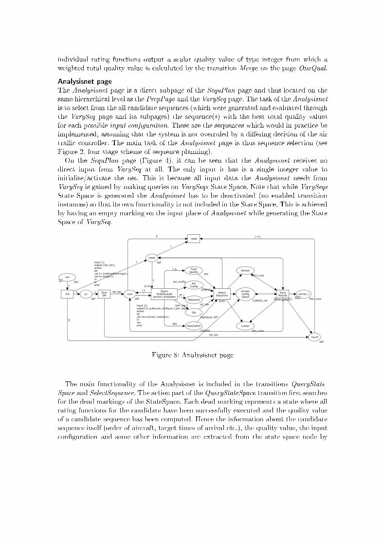
(par_sig,i)

0

1

(~1)

[]

11

1

ac_l

1act_config

i-1ilist_len

des

t_q

reset

Init SaveResults

Save Results

SelectSequence

Eval

NumDM

[i>0]

Sig

Signature_INT

count

INT

p1

INT Sequence

AC_list

winner_cOut Win_Loos

ready

INT

Looser

Win_Loos

Winner

Win_Loos

KnownConfigSpace

CONFIG_list

ActConfig

CONFIG

num

INT

initIn INT

Description

STRING

TotalQuality

INT

In

OutEval

list_len

Save Results

QueryStateSpace&

extract candidates

input (i);output (t_q,des,act_config,ac_l,par_sig);actionletval res=extract_results(i);inresend;

1input ();output (list_len);actionletval li= ListDeadMarkings();val le=length li;inleend;

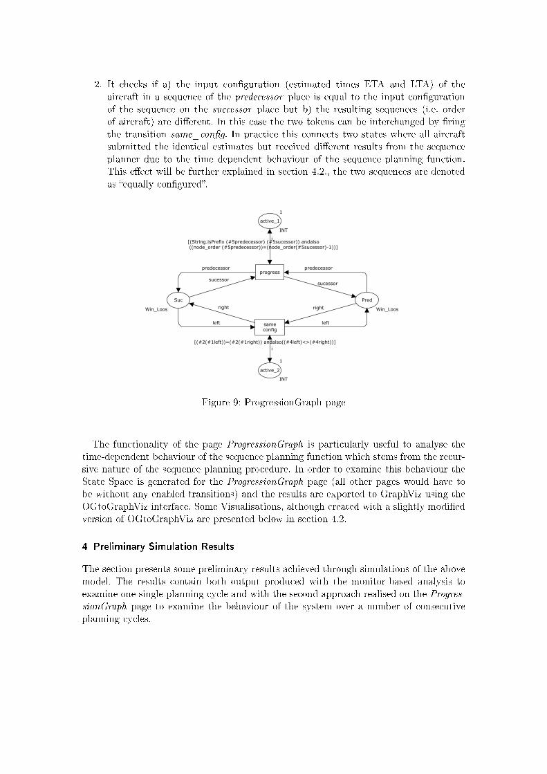
predecessor

i

left

right right

left

sucessor

predecessor

sucessor

i

active_2

1

INT

Pred

Win_Loos

Suc

Win_Loos

1

INT

active_1

sameconfig

progress

[(String.isPrefix (#5predecessor) (#5sucessor)) andalso ((node_order (#5predecessor))=(node_order(#5sucessor)-1))]

[(#2(#1left))=(#2(#1right)) andalso((#4left)<>(#4right))]

delta eta ∈ {−90,−60,−30, 0, 30, 60, 90}

delta eta ∈ {−60, 0, +60} delta eta ∈ {0, +60}

•

•

•

•

ABC

ABC

ACB

B-> eta:60 A-> eta:(~60)

BAC

B-> eta:(~60)

CAB

B-> eta:60 A-> eta:60

ABCA-> eta:(~60)

ABC

B-> eta:60

B-> eta:(~60) A-> eta:(~60)

ABC ACB

ACB

ABC

BCA

CAB

ABC

ACB

ACB

ACB

BCA

ABC

BAC

BCA

CAB

CAB

CBA

B-> eta:60

A-> eta:60

B-> eta:60 A-> eta:60

CAB

ABC

ACB

ABC

CAB

ACB

CAB

A-> eta:60

B-> eta:60

B-> eta:60 A-> eta:60

A-> eta:60

B-> eta:60

B-> eta:60 A-> eta:60

B-> eta:60 A-> eta:60

A-> eta:60

B-> eta:60

A-> eta:60

B-> eta:60

B-> eta:60 A-> eta:60

A-> eta:60

B-> eta:60

B-> eta:60 A-> eta:60

A CPN Model of a SIP-Based Dynamic Discovery

Protocol for Webservices in a Mobile Environment

Vijay Gehlot and Anush Hayrapetyan

Center of Excellence in Enterprise Technology

Department of Computing Sciences

Villanova University, Villanova, PA 19085, USA

[email protected], [email protected]

Abstract

The Session Initiation Protocol (SIP) was conceived for internet telephony. Owing to its simplicity,flexibility, and reuse capability, SIP is now viewed as an enabler of converged communications across dis-tributed networked entities. In addition, several other protocols or applications have been defined in termsof the basic SIP components. Of particular interest to us is the SIP-based Discovery protocol that has beendeveloped for the Multi-Channel Service Oriented Architecture (MCSOA). MCSOA is an enhanced Ser-vice Oriented Architecture (SOA) geared towards the Net-Centric Enterprise Solutions for Interoperability(NESI) initiative of the US Department of Defense (DoD) and Defense Information Systems Agency (DISA).The Net-Centric Enterprise Services (NCES) defined by NESI are a set of net-centric services, nodes, andutilities for use in DoD domain and mission-related enterprise information systems. The purpose of theMCSOA Discovery protocol, when compared to the traditional SOA/UDDI (Universal Description, Discov-ery and Integration) approach, is to enable location transparency, availability awareness, service guarantees,context-based routing, and fault-tolerance. In this paper we give details of a CPN model of the MCSOADiscovery protocol. The work presented is part of a larger project to integrate a CPN-based model-drivenapproach into MCSOA software development. We also briefly discuss our experience with the CPN Tools inthe context of this project.

1 Introduction

Service Oriented Architectures (SOAs) are attractive for enterprise systems because of their inherent loose cou-pling and reusability aspects. In order to capitalize on the flexibility and interoperability afforded by SOAs, theUS Air Force Electronics Systems Center and the Defense Information Systems Agency undertook a collabora-tive initiative to define a framework known as Net-Centric Enterprise Solutions for Interoperability (NESI). It isenvisioned that NESI will add value not only to day-to-day enterprise-level business operations but also to com-mand and control as well as logistics and warfare. Figure 1 gives an instance of this broad scale interoperabilityand integration proposed under the NESI initiative [15].

These data interoperability capability requirements coupled with specific defense needs add a new dimen-sion to conventional SOAs. In particular, SOAs for defense must be able to address the following:

• Service guarantees

• Fault tolerance

• Dynamic service discovery

• Interoperable multiple connection types

• Availability awareness

• Load balancing

• Security

Figure 1: Node interoperability in NESI Net-Centric Enterprise Architectures.a

aThe depicted Global Information Grid (GIG) is the future US DoD transport mechanism that will include an integratedheterogeneous network consisting of the mobile and fixed networking components at ground-based, air-based and space-basedlocations.

To address these needs, Gestalt LLC, a defense contractor, proposed a Multi-Channel Service Oriented Ar-chitecture (MCSOA) [14]. Born out of this effort was a Villanova University research project called ARCES(Applied Research for Computing Enterprise Services) to integrate a model-driven approach into MCSOA soft-ware development and to provide capabilities for system analysis. Our decision was to use Colored Petri Nets(CPN) for this purpose [8]. What sold the idea to our sponsors was extensively documented work by otherresearchers in the industrial uses of CPN in various large-scale real-life systems including military systems [13].In addition, CPNs are well supported by the great deal of theoretical research that has gone into defining them,the associated analysis techniques developed for them, and the CPN Tools system that allows flexible experi-mentation with them. Finally, availability of an active CPN Tools support team at the University of Aarhusworked towards our advantage. In this paper we give details of a CPN model of the MCSOA Discovery protocolthat was created as part of our initial efforts to integrate CPN into MCSOA development. CPNs have beenused to model a variety of protocols. For example, see [9], [5] and [1]. However, to the best of our knowledge,there have been no reported CPN models of SIP or SIP-based protocols to date.

The remainder of this paper is organized as follows. The next section contains some details of theMCSOA architecture, the Session Initiation Protocol (SIP) Presence model and the MCSOA Discovery protocolthat is built on top of it. Section 3 contains details of our CPN Discovery model. We present our conclusionsin Section 4 where we also briefly discuss our experience with the CPN Tools in the context of this project.Finally, to enhance readability, we provide a list of abbreviations used throughout the paper in Appendix A.

2 MCSOA, Presence and Discovery

From a software point of view, MCSOA is an implementation of a SOA. It can be viewed as a development,deployment, and discovery framework for SOA applications. There are three main components of a SOA:

1. The Service Provider publishes and makes a service available.

2. The Service Consumer invokes and uses a service.

3. The Service Discovery mechanism maintains information about services and their providers and allows fordiscovery of services.

The conventional webservices based view of a SOA uses HTTP/SOAP for transport and communications, andthe discovery mechanism is based on the UDDI framework which makes it static [6]. This structure is toorestrictive for general defense applications where multiple protocols and transport mechanisms are used for a

Figure 2: The MCSOA Node Architecture.

variety of communications. MCSOA solves this multi-channel problem by defining a node and a fixed intra-nodal transport mechanism and providing appropriate wrapper mechanisms for different channels. Providersand consumers of services connect through a MCSOA node. MCSOA’s internal transport is based on the SessionInitiation Protocol (SIP) [17, 2]. Since SIP is essentially a signaling protocol, using it as a wrapper poses notechnical difficulties. Furthermore, there is also an added benefit of using SIP: MCSOA is able to leverage SIP-based Presence capabilities [3] to define its dynamic discovery mechanism. To be able to do dynamic discoveryand to provide other facilities, MCSOA adds the following fourth component to the basic above listed repertoireof SOA components:

4. The Service Broker is an intermediary between a service consumer and a service provider.

In MCSOA architecture, the broker is part of a MCSOA node. Several MCSOA nodes can be connected toeach other forming a MCSOA fabric. The fabric is a dynamic concept in that new nodes may join the fabricthrough the MCSOA discovery process. Furthermore, the services available at a given node may also changedynamically. For example, a surveillance aircraft connected to, say, node A, moves out of range and reconnectsto, say, node B, to provide the same set of services. This detachment and re-attachment is handled by theunderlying SIP protocol.

The SIP architecture used for Presence consists of the following three entities [4]:

1. Presentity is the provider of presence information, that is, an entity for which presence information isbeing tracked.

2. Watcher is the consumer of presence information, that is, an entity interested in presentity status infor-mation.

3. Presence Server maintains and manages presence information, that is, it keeps track of presence informa-tion of presentities and sends notifications to watchers of the changes in status.

Figure 2 depicts the internal organs of a MCSOA node. A complete description of this architecture isbeyond the scope of this paper. In this figure, the component named Prospector/Presence Server implements theSIP Presence Server capabilities. Internally SIP messages are used to establish subscriptions and to communicatepresence changes. SIP REGISTER messages are used to establish initial contact with MCSOA. Under SIP,registration creates basic presence information and is handled by a special entity called Registrar (componentlabeled Perspective Manager in the figure). In MCSOA, as is typically the case in most SIP-related presence

Figure 3: MCSOA Dynamic Discovery Process.

models, the Presence Server and the Registrar are co-located. SIP NOTIFY messages are used to communicatepresence information to Watchers. SIP SUBSCRIBE messages are used to declare an interest in presenceinformation for particular presentities. Watchers send SUBSCRIBE messages to the Presence Server. ThePresence Server sends a SIP NOTIFY response for each subscription request initially as well as whenever thereis a change in the status of the subscribed presentity. Presentities send REGISTER messages to the PresenceServer. Registration is processed by the Registrar component. The Registrar notifies the Presence Server whena presentity’s presence status changes. Both the SUBSCRIBE and the REGISTER requests carry an expirationtime. An entity may re-SUBSCRIBE or re-REGISTER.

The components Perspective Manager, Discovery Manager, and Subscription Agent shown in Figure 2provide the discovery capability. Discovery is the process of finding a service provider for a consumer request.There are three possible situations for a request:

1. Consumer bob@node1 is looking for service provider alice@node1. In this case the request is for a serviceat the local service access point. This case is handled by simply doing a lookup of the local registrationtable.

2. Consumer bob@node1 is looking for service provider alice@node2. In this case the request is for a serviceat the remote service access point. This case is handled by simply forwarding the request to the remotenode. Thus, effectively, the local node acts as a SIP Proxy Server in this case [17, 2].

3. Consumer bob@node1 is looking for service provider alice. This constitutes a request without specificservice endpoint and triggers the MCSOA discovery process depicted in the flow diagrams in Figure 3. Asshown, it is a two step process:

(a) The first step corresponds to intra-nodal activities and is termed Broker Work Flow in the diagram. Inthis case, the service Broker first consults the Perspective Manager/Registrar for service availability.This step may succeed owing to a previous discovery process or because of a local provider beingavailable in the local registration table.

(b) The second step is executed if the first one fails. This corresponds to inter-nodal activities and istermed Fabric Work Flow in the diagram. In this case, the service Broker consults the Prospec-

tor/Presence Server and uses its Discovery Manager to locate candidate providers for the desiredservice. This may yield zero or more candidate Service Access Points (SAPs). For each providerSAP, the Subscription agent interacts with the Perspective Manager of the remote node to subscribeto remote provider. Again this step may or may not succeed. In case of a success the local Per-spective Manager updates the registration table with information about non-local providers of theservice and forwards the request to the remote provider. Otherwise, a failure message is returned tothe consumer.

In summary, when a request without specific service endpoint is received and such a service is not locallyavailable, then the local node essentially becomes a watcher for the presence information of the service providerby making use of the underlying presence capabilities of each MCSOA node. The initial contact points may beobtained via a UDDI or any other location service lookup. Rediscovery may be avoided by updating the localregistration table based on presence information gathered during the discovery process. We would like to pointout that the simplicity of the work flows depicted in Figure 3 can be misleading, for, as we shall shortly see, theunderlying details of this process are quite involved.

It should be clear from the discussion above that Presence is a crucial part of the Discovery process. Webuilt a CPN model of Presence before we built the Discovery model. Details of the CPN Presence model aredescribed in [7]. In the next section we present our CPN model of the Discovery process which is the focus ofthis paper.

3 CPN Discovery Model Description

This section presents a description of our CPN Discovery model. We start by giving a high level overview of thestructure of the model in the first subsection. The remaining subsections give a more detailed description of theindividual components making up the CPN Discovery model. Due to space limitations, a detailed descriptionof some of the lower-level entities of the model will be omitted.

3.1 Hierarchy

The Discovery CPN model consists of five main components: two User Agents, two MCSOA nodes and oneNetwork and Routing component. Each User Agent is connected to a MCSOA node, which is responsiblefor processing the messages received from that User Agent. The two MCSOA nodes can also communicatewith each other so as to enable them to use each others’ services. The Network and Routing componentensures the communication between the User Agents and the MCSOA nodes, as well as that between the twoMCSOA nodes.1 Each of these five components contain further subcomponents, called modules or pages, whichimplement specific functionalities of the component. These pages may further contain subpages, thus creatinga natural hierarchical structure for the Discovery CPN model. There are a total of 73 pages in the DiscoveryCPN model, each corresponding to a line in Figure 4.2 The page Top is the outermost module of the hierarchy.Many pages have substitution transition(s) [8]. In the figure, such pages contain a “V” before their name. Wewill describe substitution transitions in more detail later.

The five components of the Discovery CPN model are identified as: User Agent 1, MCSOA Node 1,User Agent 2, MCSOA Node 2 and Network and Routing. The pages corresponding to these five componentsdirectly descend from the page Top. The two User Agent pages SIPUserAgentsN1 and SIPUserAgentsN2,which are not visible in Figure 4, are responsible for sending registration (REG) requests for both consumersand providers, subscription (SUB) and message (MSG) requests from consumers to providers and notification(NTF ) messages to either consumers or MCSOA nodes. Each message has an automatically generated uniquecall ID (as required by SIP [17]) associated with it, which is used to identify the responses for that mes-sage. SIPUserAgentsN1 communicates with MCSOANode1 page and SIPUserAgents2 communicates withMCSOANode2 page through Network and Routing component. The main purpose of the MCSOA nodes isto handle the REG, SUB, MSG and NTF requests:

1. Registration : Each time a MCSOA node receives a registration request, it adds the entity to its localregistration table REGTableN1. If the entity is already present in REGTableN1, the local informationabout that entity gets updated. Also, a timer corresponding to each register request is set to expire

1In the future, the functionality of the Network and Routing component can be extended to include additional features, such asconverting messages from one type to another, or message compression and decompression.

2We did not display the full hierarchy, since it would take too much space. We only included the structures of one of the MCSOAnodes and the Network and Routing component.

�� !�� !��"�� #�� !�� !��$�� !��$�� %�� %��%��&��%�� " �� $��"� ��&�� & ��&�� &�� &�� &�� &��&��&�� &�� !��&�� !�&�"�� #�� !�&�� &�� &!��$�� &� �� &�� &!��$�� &%�� &��%��&�&��%�� &��%� ��&��" �� &�� &��"#��&��"#�� &�� !�&��&��&�� &�� &�� &�� &� �� &�� "#��"#�� !��

· · ·

Figure 4: The partial hierarchy page — overview of the CPN Discovery model.

after the period of time specified by the expiration parameter of that REG request. When the timerexpires, the corresponding entity is removed from the local REGTableN1 and becomes unknown to theMCSOA node.

2. Subscription : When a MCSOA node receives a subscription request, it adds the subscription to itsSUBList table and sets a timer for that subscription. It also sends a response to the source of the SUBrequest with the same call ID as that of the incoming request, and a response code of 200 [17]. Thepurpose of a subscription message is to express interest in the presence information of a particular provider.Thus, after sending a subscription request, the consumer waits for a notification message NTF about thestatus of the provider. This message lets the consumer know whether or not the provider is registered,and also contains the time that remains before the expiration of the subscription. When the status of theprovider changes, notification messages are sent to all consumers which have unexpired subscriptions inthe SUBList table for that provider. When the registration time of the provider expires, all subscriptionsfor that provider are removed from the SUBList and put into the PendingSUB list. The latter stores thepending subscriptions for a provider.

3. Message : Handling MSG requests is the main task of the Discovery model. Two types of MSGmessages can be received on each of the two MCSOA nodes - MSG with a specific service end pointand MSG without a specific service end point. MSG with a specific service end point is used when thedestination of the message, i.e. the MCSOA node for which the message is designated, is known inadvance. In this case the MCSOA node, corresponding to the User Agent sending the MSG request,forwards the message directly to the destination MCSOA node. If the message is designated for the localMCSOA node, then it gets processed locally. MSG without a specific service end point is used whenmessages are not intended for any particular MCSOA node. In this case, the MCSOA node receiving themessage consults its local REGTable first. If the provider specified in the message is found in the localMCSOA node, then the MCSOA forwards the message to the corresponding User Agent and waits fora response. Otherwise, a Discovery Process is triggered, during which a global static table (UDDI or anyother suitable location server) is consulted to find a MCSOA node where a provider might be registered.If a provider is not found in the UDDI, a response with code 480 [17] is sent back along the reverse pathto the source of the message. If the UDDI contains at least one record of that provider, the message isforwarded to the MCSOA node indicated by the UDDI for processing.

The messages exchanged among the various components of the Discovery model follow the SIP “format”of a message. The colorset SIPMsg associated with a message is of the form:

colset SIPMsg = union SIPReq : SReq + SIPResp : SResp;

��

��

��

�� !��"�� !��"��

��

��#� ��#�� $� ��%��

#��&��'��'�#��&��'��'�

#��&��'��'�#��&��'��'�

��'�#��&��'��'�#��&��'� ��'�#��&��'��'�#��&��'�

�� #�� $�

�� !��"��

��

��

Figure 5: The Top page.

where

colset SReq = product CallID * FromNodeID * ToNodeID * SIPMethod *SIPBody * MsgSize * Expire;

colset SResp = product CallID * FromNodeID * ToNodeID * SIPRespCode* SIPBody * MsgSize * Expire;

Here we skip the explanation of the various other colorsets and functions declared in the model in order to keepthe paper within the page limits.

3.2 The Page Top

Figure 5 depicts the page Top, which is the first page of the Discovery CPN model hierarchy (see Figure 4).The ellipses in the figure are called places and are used to model the states of the net. The rectangles inthe figure are called transitions. The state of the CPN model is called a marking and is a distribution oftokens on the places of the CPN model. The Top page captures the high-level overview of the model and theaforementioned five primary components - User Agent 1, MCSOA Node 1, User Agent 2, MCSOA Node 2,and Network and Routing - correspond to the five large transition boxes in the figure. Below each largetransition box, there is a smaller box, implying that these transitions are substitution transitions associatedwith the page named in the smaller box. From now on, we will refer to such transitions and their correspondingpages interchangeably. Also on the page Top, there is a transition to populate the place UDDI. This transitionis enabled immediately after the Start page completes the initial loading of the input data from various inputfiles.

3.3 The Description of the MCSOA Node

We now describe the structure of the first MCSOA node. The second one is analogous, hence we will omitit. We present only those components from Figure 2 that participate in the Discovery process, namely, Per-spective Manager, Broker Discovery Manager and UDDI. We will initially give a high-level description of theMCSOA node, and then continue with a detailed description of the components making up the MCSOA nodeas depicted in the hierarchy shown in Figure 4. This structure of presentation will be used for the remainingcomponents of the Discovery model as well.

��

�� !"#$%$&'( �� ( �)��

*��((+� �� ( � �� *��, �� ( � �( ��- � .*��, �� /� �( �� *��, �� ( � �( ��- � .*��, �� /� �( ��/�( �

�/�( �(+��

Figure 6: The MCSOANode1 subpage of Top page.�� !�� !�

"�� !�"�� !��#$�� %& �'() �� *+�� &,�� !�

"��&,��&�� !��&,�� !�"��&,��&�� !�&�� &�� %&

� �� Figure 7: The PerspectiveManagerN1 subpage of MCSOANode1 page.

3.3.1 The MCSOANode1 subpage of Top page

Figure 6 depicts the page MCSOANode1. A MCSOA node consists of two main parts — Perspective Manager(PM) and Broker Discovery Manager (DM). The Perspective Manager is responsible for handling REG andSUB requests and is designed according to the requirements of the Presence Model that are described in [17].The Broker Discovery Manager handles the MSG requests, both with and without a specific service endpoints. Notice that the place REGTableN1, the local registration table of MCSOANode1, is connected toboth the PM and the DM , whereas the UDDI is connected only to the DM , since the latter handles thediscovery triggered by MSG messages. The place REGTableN1 is connected to the PM , since the PM needsto update it when a new registration or the expiration of a registration occurs. Also, the PM needs to consultREGTableN1 when a SUB message is received in order to find whether the provider mentioned in the SUBmessage is in REGTableN1 or not. On the other hand, the DM needs to consult REGTableN1 during localrouting (i.e. routing where destination MCSOA node is the same as the source MCSOA node). The other fourplaces ensure the communication between MCSOA Node 1 and other components of Discovery CPN model.

3.3.2 The PerspectiveManagerN1 subpage of MCSOANode1 page

Perspective Manager (PM) is the part of a MCSOA node where registration and subscription messagescoming from the User Agent are handled and notification messages are generated (see Figure 7). The work-load of the PM is distributed among its three subpages, corresponding to the large boxes in the figure.The ClientTransactionN1 and ServerTransactionN1 subpages, which are located on the right side of thefigure, assure SIP-compliant communication between MCSOA Node 1 and the other components of theDiscovery model.3 All registration, subscription and notification messages that go through the Client andServer Transaction subpages are generated and analyzed in the RegistrarAndPresenceServerN1 page.

3SIP − compliant communication means that in order to pass a message from one place to another, the message has to passthrough the Client Transaction on the source side, and be received by the Server Transaction on the destination side. Theresponse for that message travels from the ServerTransaction on the destination side to the ClientTransaction on the source side.

��

��!"� �� !"� ��

��#$��%! �&'(��)� �� %!!"�!"�

��

�� * �� * �� * ��Figure 8: The RegistrarAndPresenceServerN1 subpage of PerspectiveManagerN1 page.

3.3.3 The RegistrarAndPresenceServerN1 subpage of PerspectiveManagerN1 page

The page RegistrarAndPresenceServerN1 (Figure 8) is responsible for handling REG and SUB messagesoriginating from User Agents which have already passed through the Server Transaction of PM . The arcmarked REG in the figure signifies that registration requests are handled by the RegistrarN1 page. Similarly,the arcs marked SUB and NTF imply that subscription requests are handled and notification requests aregenerated in the PresenceServerN1 page. Furthermore, the RegistrarN1 and PresenceServerN1 pages arealso connected with each other via the NewREG and ExpREG places. When a new registration request fora provider is received by the Registrar, in addition to updating its registration table and putting a timer forthat message, the Registrar also passes that request to Presence Server, which moves all the subscriptionsfor that provider from PendingSUB to SUBList (not shown in Figure 8 since they are part of the subpages ofthe depicted RegistrarAndPresenceServerN1 page). When an expiration event occurs, a token is passed throughthe ExpREG place to the Presence Server. If a consumer’s registration expires, then its all subscriptions areremoved from both PendingSUB and SUBList tables. If a provider’s registration expires, all the subscriptionsfor that provider are moved from the SUBList table to the PendingSUB table.

3.3.4 The RegistrarN1 subpage of RegistrarAndPresenceServerN1 page

The RegistrarN1 page (Figure 9) describes the actions taken when a new registration for either a consumer ora provider arrives. The registration message is of the form SIPReq(cid, fr, to, m, b, s, exp) explained earlier inthe paper, where cid is the callID of the message, fr and to are the source and the destination of the message,m denotes the type of the message and is equal to REG for registration messages, b is the body of the messageand is empty for registration messages, s is the size of the message and finally exp is the expiration time. Whena registration message is received, the AcceptREGSendOK transition becomes enabled.

After firing the AcceptREGSendOK transition, a response is generated with the call ID equal to that ofthe original registration message. This response is then sent through the Server Transaction of the Registrarto User Agent 1 with the success code 200 [17]. Meanwhile, a timer is set for the entity’s registration, whosevalue is taken from the exp parameter (expiration time) of the REG message. This is done by putting a timedtoken in the place Timer with a time stamp equal to the registration expiration time.

In addition, firing the AcceptREGSendOK transition puts a token in the place NewREG whenever theentity that just registered is a provider. As was mentioned in the previous section, that token will be passedto the Presence Server in order to update the contents of the SubList and PendingSUB tables. Notice, thataccording to the SIP requirement document [17], there is no need to send consumers’ registration messages tothe Presence Server, because the subscriptions are moved between the PendingSUB and SubList tables onlywhen providers register or unregister.

Finally, firing the AcceptREGSendOK transition updates the content of the REGTableN1 by deletingany previous registration of the newly received entity and adding the ID of that entity in REGTableN1. Theexpression assigned to the incoming arc to the REGTableN1 ensures that the same entity will not appear inthe REGTableN1 more than once, even when more than one registration or unregistration requests are receivedfor that entity.

��

��

�� ! �� " � �� # ��$�� %!!�&��$��'�� &��

� �� # �� "��

(��)*$��+,- �)*. �� /�� %!!�/0��

1��)*��&��)*��&��2��3+ -.��2��45��

)��)*+�� 2��4)�� )��

5��)�� )* -.��)�� 5�� )��6�2�7�)*+�� 2��4 0�� (��$�+�� $��6�0�� $��(� $��6�� +��+��

+��

�3+

Figure 9: The RegistrarN1 subpage of RegistrarAndPresenceServerN1 page.��

�� !� "�� # $ ��% �� # $�� !� "&�� '�()�� &*�+� �� '�()� � &��+� �� '�()�!� "&*� � �� '�()�� +��+� � ��

�� Figure 10: The PresenceServerN1 subpage of RegistrarAndPresenceServerN1 page.

The LastEnteredREG table is a list which keeps the information about consumers, providers and theirregistration expiration times. The incoming arc expression puts the latest information about entities and theirexpiration times in the LastEnteredREG table.

When there is a token in the place Timer with the time stamp less than or equal to the current time, thetransition Fire becomes enabled, which, when fired, puts all the expired tokens in the place Expired. Firing thetransition ChangeREGTable checks whether there is an entity in the LastEnteredREG table with the sameID number and expiration time as the one in the place Expired. If such an entity is found, then it is deletedfrom the LastEnteredREG table. The same entity is also deleted from the REGTableN1 and a token withthe expired entity’s ID number is put in the place ExpREG and passed to the Presence Server.

3.3.5 The PresenceServerN1 subpage of RegistrarAndPresenceServerN1 page

The page PresenceServerN1 (Figure 10) consists of two main components — ProcessREGInfoN1 andProcessSUBInfoN1. ProcessREGInfoN1 is the page where new and expired registrations coming fromthe Registrar are handled. ProcessSUBInfoN1 is activated when subscription messages from User Agentsand MCSOA nodes are received. This page is also responsible for setting timers for subscriptions and sendingnotification messages back to the consumers.

Observe that there is a communication between ProcessREGInfoN1 and ProcessSUBInfoN1 viathe SendSUB place. According to the Presence Model requirements [3, 4], when a consumer unregisters,it must also unsubscribe. Hence, when the registration of a consumer expires, ProcessREGInfoN1 sendsunsubscription requests (subscription request with expiration time equal to 0) for that consumer. As a result,all (consumer, provider) pairs, whose first components is the unregistered consumer, are removed from theSUBList and PendingSUB tables.

�� !��

��!��

��"�� #��"�� #��"�� # ��$��"��#��"��#��"��#Figure 11: The ProcessREGInfoN1 subpage of PresenceServerN1 page.��

�� !" �#$% �� &'��

��(�� )�� )��)�� *�+,� ��-"� � �*�+,��"� � �*�+,� )��- � � �*�+,� �"�

"� � � !"�� (��(��(��

Figure 12: The ProcessSUBInfoN1 subpage of PresenceServerN1 page.

3.3.6 The ProcessREGInfoN1 subpage of PresenceServerN1 page

The page ProcessREGInfoN1 (Figure 11) consists of two subpages — ProcessNewREGN1 and ProcessEx-pREGN1. The first subpage updates the SUBList and PendingSUB tables when a new registration of aprovider arrives from Registrar. The second subpage updates those tables when an entity’s registration ex-pires. Both of these subpages are connected to the Client Transaction via the ToUAC and FromUAC places.When some changes occur in SUBList and PendingSUB tables, notification messages are sent to the affectedconsumers using those places.

3.3.7 The ProcessSUBInfoN1 subpage of PresenceServerN1 page

As we can see from Figure 12, the task of the ProcessSUBInfoN1 page, which was responsible for processingthe subscription messages, is divided into two parts — processing of new subscriptions (ProcessNewSUBN1)and processing of expired subscriptions (ProcessExpSUBN1). When a new subscription message comes fromthe Server Transaction (via the place FromUAS), it is sent to the ProcessNewSUBN1 page, where the re-sponse for that message is generated and sent back to the Server Transaction through the place ToUAS. TheProcessNewSUBN1 page also sends notification messages about the current status of the provider.4 The notifi-cation messages are sent to the Client Transaction residing on the Presence Server through the place ToUAC,and the responses for these notifications are received from Server Transaction through the place FromUAC.Furthermore, the SUB messages are passed to the ProcessExpSUBN1 page where a timer is created for them.As described earlier in the description of Presence Server page, when a consumer unregisters, it must also un-subscribe. The tokens corresponding to the unsubscription requests are generated in the ProcessSUBInfoN1page and put into the SendSUB place. They will get processed in the ProcessExpSUBN1 subpage.

3.3.8 The Client and Server Transactions Component

Non Invite Client and Server Transactions, depicted on Figures 13 and 14, are the most essential parts of SIPcompliant transactions. Each request in an SIP compliant model should pass through the Client Transactionof one side and be received by the Server Transaction of the other side, where the response for the requestshould be generated and forwarded back along the path through which the request came.

For a message to travel from its source to its destination, it must start at a User Agent also known asTransaction User (TU), which corresponds to the source of the message. Then it must be forwarded to theClient Transaction on the source side, from Client Transaction to Transport, then to the Server Transactionon the destination side, which in its turn finally forwards the message to the destination TU . The Client and

4Currently this message informs whether the provider is in the REGTable or not and also contains the remaining expirationtime for that subscription as per SIP specification.

��

�� !�� "#��$�� %��&��'�� %� (

�%� ( #��$�� %��&��'�� #��$ �� %�&��'��#�� &��'�� )*�� %��+��

�%� ( #��$ �� %��&��'�� )*�� #��$�� %��&��'��#��$ �� %��&��'�� #��$ �� %��&��'�� #�� ,�� ,� ��,��,�&,��,��'�,�� - �� ,� !�� "#��$ �� %�� &��'�� %� (

�%� ( �� !�� "� �� %� ()* �� %��+�� - �� !�� "#��$�� %��&��'�� %� (#�� & �� '� � #�� & �� '� � #��$�� %��&��'�� #��$�� %��&�� '�� #��$�� %��&��'��#��$�� %��&��'�� %�� )*�� %�� )*�� %��#��$ �� %�&��'�� #��$�� %�&��'��#��$�� %�&��'��

�� %� ��.� ��/� ��0��+. /� ��0�� . /� ��0 ��. /� ��0��1 ��2�1 �1 �� 2�� 3�� 2��.� ��/� ��,0

��. /� ��0��1 �� 2�1 �1 �� 2�� 3�� 2��.� ��/� �� 0��. /� ��0#��$.%45��%456+0

�%�� 1� �� #��7��8�

��%�� 1� �� 9 #��7��8�� %��+��1� �� %��(��8� �%�� 1� �� #��7��8�

��%�� 1� �� 9 #��7��8�

��%�� 1� �� 9 #��7��8�� %��1� �� %� ��(��8� � �%��1� �� %��':� 8�� #��7��8�� %��+��1� �� %� ��(��8�

� �%��1� �� %��':� 8�� %��1� �� %� ��(��8� ��( �� #��7��8��%�;�� #��7��8� �� <1 #��7��8�

��%�� #��7��8��;<1 #��7��8�<1 ��

<1 �� 1� �� 1� �� 1� �� 1� �� 1� ��

�1� �� 9

�1� �� 9�1� �� 1� �� 1� �� 9

�1� �� ,� !�� "#��$�� %��&��'�� %� (#�� ,�� ,� ��,��,�&,��,��'�,�

Figure 13: The ClientTransactionN1 page.

��

� �� !��"��#��$� �%� �#� !� &"�'() �� &�*��

��"�� #�� #��#��#��+��,"��"�� #�� #��#��#��+��,"��

��- �� #�� #��#��&��+��,"��

&"�'��"�� #�� #��#��#��+��,"�� #� () �� & �* ��"�� #�� #��#��#��+��,"��"�� #�� #��#��#��+��,"��- �� #.� ��#.��#.�&.�+.��.�,".� ��"�� #�� #��#��#��+��,"��"�� #�� #��#��#��+��,"�� "�� #�� #��#��#��+��,"��

��"�� #�� #��#��#��+��,"��"�� #�� #��#��#��+��,"��"�� #�� #��#��#��+��,"�� "�� #�� #��#��#�� +��,"��"�� #�� #��#��#��+��,"�� !��"��#��$� �%��"�� #�� #��#��#��+��,"�� !� &"�'� �� !��"��#��$� �%��"�� #�� #��#��#��+��,"�� !� &"�' ��"�� #�� #��#��#��+��,"��-�� #�� #��#��&��+��,"��- �� #� ��#��#�&�+��,"��-�� #� ��#��#�&�+��,"��- �� #� ��#��#�&�+��,"�

��*/� �#�0�1�-��#2� ��/� �#�0� �#�1�#��"2� ��/� �#�0� �#�� !��"��#��1�#�� !��"/� �#�0� �#�� !��"��#��1�-��#2� ��/� �#�0� �#.1

�#��"/� �#�0� �#�1��-/&3456�&34��1

� �&�*��7� �� &��'"8�

��&�� #�� &�*��7� �� &��'"8��&"!�#��7� �� 9 ��5��8�

��&"!�#��7� �� 9 ��5��8� ��# ��5��8��' ��5��8�

��:;7� ��5��8��&�:�� 5��8�� "� ��;7� ��5��8�

��&�� "� �� 5��8��

;7� ��;7�

�7� �� 9

�7� �� 9 �7� ��

�7� ��

Figure 14: The ServerTransactionN1 page.

��

��

��

��

��

!"#��$�� %��

� ��

�� &��'�� &��'�� &��'�� Figure 15: The BrokerDiscoveryManagerN1 subpage of MCSOANode1 page.

Server Transactions accomplish their task of delivering requests and responses using state machines, whoserequirements can be found in [17]. The Client and Server Transaction pages are essentially the result ofconverting those state machines into their corresponding CPN models. The states of the machine get mappedto places in the model with identical names. Note that the Client and Server Transactions pages are usedseveral times throughout the Discovery model. The port places FromTransport, ToTransport, FromTU andToTU get populated when messages are passed or received to or from Transport or TU . Port-socket connectiondetermines the flow in each case when the Client and Server Transactions are used and the connections canbe different from the orientation used in Figures 13 and 14. For example, in Figure 13 the port FromTU isconnected to the socket ToUAC place in Figure 7, the port ToTU is connected to the socket FromUAC, the portToTransport is connected to the socket FromUACOfNode1 and finally the port FromTransport is connected to thesocket ToUACOfNode1. Although Client and Server Transactions used throughout the model have completelyidentical structures, we could not simply use the currently available pure cloning because when cloning a pagethat contains local fusion sets, new fusion sets are not created for the cloned page. This makes pages dependenton each other, which is not desirable in our case.

3.3.9 The BrokerDiscoveryManagerN1 subpage of MCSOANode1 page

The BrokerDiscoveryManagerN1 page (Figure 15) is activated any time a MSG request or a response fora MSG request is received. The page BrokerDiscoveryManagerTUN1 is responsible for identifying thetype (with or without a specific service end point) of the message and handling it accordingly. DM alsocontains a Client Transaction in order to send or forward requests, and a Server Transaction in order tosend or forward responses for those requests. The ToUACOfNode1, FromUACOfNode1, ToUASOfNode1,FromUASOfNode1 places connect the MCSOA node 1 with the Network and Routing component of theDiscovery model. FromUAC, ToUAC, ToUAS, FromUAS places are considered local and are designated toconnect the BrokerDiscoveryManagerTUN1 subpage with the Client and Server Transactions.

3.3.10 The BrokerDiscoveryManagerTUN1 subpage of BrokerDiscoveryManagerN1 page

The BrokerDiscoveryManagerTUN1 page (Figure 16) is responsible for handling two types of tasks. Thefirst one is to find the destination of the MSG messages, i.e. discover whether the received MSG message wasintended for the local MCSOA node 1, or for the remote MCSOA node 2, or has unspecified destination. Thisis implemented in the FindDestinationN1 subpage. The second task is to pass an MSG message without aspecific service end point through the discovery process if its provider was not found in the local REGTable.This part is handled by the ConsultUDDIN1 subpage. Observe, that the place UDDI is connected onlywith the ConsultUDDIN1 transition. This reveals the fact that the UDDI should be consulted only in caseof the Discovery process. The place NotFound ensures the connection between the two described subpages.When a MSG message without a specific service end point is received and the provider is not found in theREGTableN1, a token is put in the NotFound place and passed to the ConsultUDDIN1 subpage. The placesFromUAC, ToUAC, ToUAS, FromUAS are designed to pass the tokens for MSG requests and their responsesto FindDestinationN1 and ConsultUDDIN1 subpages.

�� !��" �� ! �� #� �� $%� ��&�� # �� &� ��# �� ' (�� #� �� #�� $%� ��&�� # ��) �� '��# ��)��# ��)��

��#�� )*��+��!�)� �)*��+�$%��&��), )��)-��!�)� �)*��+� �)), ��)��!� #� �)*��+��!� #� �)*��+� #� #� ), )�

), )�

��# ��)��

Figure 16: The BrokerDiscoveryManagerTUN1 subpage of BrokerDiscoveryManagerN1 page.�� !� "��

#$��%�� &� �� '� �� !� "��

��(�� !� "�� !� "��

��(�� !� "��

��

��

&��

Figure 17: The FindDestinationN1 subpage of BrokerDiscoveryManagerTUN1 page.

3.3.11 The FindDestinationN1 subpage of BrokerDiscoveryManagerTUN1 page

The FindDestinationN1 page (Figure 17) describes how the destination of the MSG message is determinedwhen it is received by MCSOA node 1. The destination parameter of the MSG request is a pair whose firstcomponent is the ID of the provider for which the MSG message is intended and second component representsthe end point of the MSG message and can be either 0, 1 or 2. According to the convention used in theDiscovery model, if the value of the end point is 1, then the MSG message came for MCSOA node 1. In thiscase, the local REGTable is consulted to find whether the provider exists. If the provider is not found, a responsewith code of 480 is generated. Otherwise the message is forwarded to the User Agent and the MCSOA nodewaits for a response from that User Agent. This functionality is handled in the subpage MSGForNode1N1. Ifthe value of the flag is 2, MCSOA node 1 forwards the message to MCSOA node 2 — the intended recipient —without consulting either the local REGTable or the UDDI. MCSOA node 1 then waits for a response fromMCSOA node 2. This case is handled by the MSGForNode2N1 subpage. Finally, when the value of the endpoint is 0, the provider is unspecified and must be discovered. According to the Discovery model requirementdocument [14], in this case the local REGTable is consulted first. If the search is unsuccessful, the UDDI isconsulted next. If the UDDI finds that the provider is available on MCSOA node 2, the message is forwardedto MCSOA node 2. Otherwise, a response with the code 480 is generated and sent back to User Agent 1. TheMSGForAllN1 subpage is responsible for handling this last case.

3.3.12 The ConsultUDDIN1 subpage of BrokerDiscoveryManagerTUN1 page

The main task of the ConsultUDDIN1 page (Figure 18) is to consult the UDDI when a token corre-sponding to an MSG message appears in the place NotFound, implying that the provider was not foundin the local REGTable and the message was forwarded to the ConsultUDDIN1 page. Firing the transition

��

�� !��" ��

�� #$ �� %%�� !�� &� '&��

��(�� ) *�� ( �� ) *�� +�� ( �� ,��$�� "�� ) *�� !��"

�� +�� !��"� ��

�� #$ �� ( �� ) *�� !��" ��( �� -��

�� +�� ,��+ �� !��"�� +�� (�,��+ �� ,��$�� " �� .�� /��// � �� !��" �� ( �� ) *��

�0-� �) *1� �� 2//3

*��-4 ��#$ 1� ��3 �� 5+�� 2//�67/ 5�0-� � �.1� �� 3

�� 5+�� 67/ 5�$*�+��8� ��9�� + �� +�� -�� + ��:�

+;�) * �)�,:� <+ �� -��0�+ ��-��!�= � �)�,:�

�8� ��=�� )�,:��= �� )�,:� -��!�=�� )�,:�

��-�� )�,:��

��

�� 8�

�

-�� 8�

Figure 18: The ConsultUDDIN1 subpage of BrokerDiscoveryManagerTUN1 page.

ConsultUDDIN1 tries to find a pair in the UDDI whose first component is the provider appearing in theMSG message. If such a pair is not found then a response with code 480 is generated and a token correspondingto the response is put in the place ToUAS. Otherwise, the second component of the pair from the UDDI willindicate the MCSOA node, on which, according to the UDDI, the provider might be registered. In this case, aSUB message is sent in order to subscribe MCSOA node 1 for the provider on the other MCSOA node. Whena response for SUB requests is received, the place FromUAC gets populated and the transition OKForSUBbecomes enabled. Firing it will remove the response token from the place FromUAC as well as the token withthe same value as the cid parameter of the response message from the place WaitForOK.

When a notification message is received from the other MCSOA node by MCSOA Node 1, the transitionGetNTFwithY ES becomes enabled. Firing this transition will check the value of the body (b) parameter ofthe notification message. If the value is NO, it means that the provider was not registered on the otherMCSOA node and the information derived from the UDDI was incorrect. If the body parameter is Y ES,firing the GetNTFwithY ES transition will forward the MSG message to the other MCSOA node. In bothcases firing the transition GetNTFwithY ES will generate and send a response for the notification message tothe other MCSOA node.

3.4 The Network And Routing Component

The Network and Routing component is the second main component of the Discovery CPN model, and isresponsible for handling all the communication between the User Agents and the MCSOA nodes forming theMCSOA fabric (see Section 2). In this section we will go into the details of the design of this component. Asbefore, the first subsection will give an overview of the component, while each of the remaining subsections willdescribe a particular module of the component. Due to space limitations, our description will be high level, andmany details will be omitted.

3.4.1 The NetworkAndRouting subpage of Top page

The NetworkAndRouting page (Figure 19) is responsible for the communication between each User Agentand its corresponding MCSOA node, as well as that between the two MCSOA nodes. In our model, thesubpage Node1UA ensures the communication between User Agent 1 and MCSOA node 1, the subpageNode1Node2 handles the communication between the two MCSOA nodes, and finally the subpage Node2UAenables the communication between User Agent 2 and MCSOA node 2. The places around the substitutiontransitions in Figure 19 are port-socket places and get populated from the Client and Server Transactions ofthe corresponding Discovery model component/subpages.

3.4.2 The Node1UA subpage of NetworkAndRouting page

The Node1UA page (Figure 20) models how SIP requests and SIP responses are passed between outgoing placesof User Agent 1 and the incoming places of MCSOA node 1. Notice that the direction of the messages aredetermined by the fr and to parameters of the request message. Also, the conditions imposed on the transitionsensure that the messages are forwarded along the proper direction.

��

��

��

��

�� Figure 19: The NetworkAndRouting subpage of Top page.��

�� !!��!�"#$��%�&

�� !!��!$"#$�� %�&��!!� !�"#$��%�&��!!� !$"#$�� %�& �� '�� (��)!!� � '��'*� ��(��)!!� ��'��'*� ��(��)!!� � '��'*� ��(��)! �� '�� (��)!!� ��'��'*� ��(��)!�� '�� (��)!�� '�� (��)!�� '*��'*�'*�'*��

Figure 20: The Node1UA subpage of NetworkAndRouting page.

3.5 The User Agent Components

The final main components of the Discovery model are the User Agents. In the following subsections we willgive a detailed description of the design of the User Agent 1 component. The User Agent 2 is analogous.

3.5.1 The SIPUserAgentsN1 subpage of Top page

The page SIPUserAgentsN1 shows the high-level functionality of the User Agent 1 component. As can beseen from Figure 21, User Agent 1 consists of the two main types of entities — consumers and provides. Thefour places on the page are used to connect User Agent 1 to the Network and Routing component. Notice,that while consumers can send REG, SUB and MSG messages and receive NTF messages, providers can onlysend REG messages. The arcs in the figure that do not have auxiliary text on them are designated for receivingresponses for REG, SUB and MSG messages and sending responses for NTF messages.

3.5.2 The ConsumerN1 subpage of SIPUserAgentsN1 page

Figure 22 depicts the structure of the page ConsumerN1. Its three subpages — ClientTransactionN1,ServerTransactionN1 and ConsumerTransactionUserN1 — are responsible for sending REG, SUB, andMSG messages to MCSOA Node 1. As was discussed above, the ClientTransactionN1 and ServerTrans-actionN1 pages ensure SIP compliant communication. The page ConsumerTransactionUserN1 is the placewhere all the messages are generated and is also responsible for matching the responses for these messages to theirsources. The FromUACOfAgentN1, ToUACOfAgentN1, ToUASOfAgentN1 and FromUASOfAgentN1places get populated when a message request moves between the Client and Server Transactions and theNetwork and Routing component. On the other hand, the FromTUToCT , FromCTToTU , FromSTToTU ,FromTUToTST places store tokens that move between the Client and Server Transactions and the Con-sumerTransactionUserN1 transition.

3.5.3 The ConsumerTransactionUserN1 subpage of ConsumerN1 page

The main task of the ConsumerTransactionUserN1 page (Figure 23) is to send REG, SUB and MSGmessages. These functionalities are implemented in the SendREGN1, SendSUBN1, SendMSGN1 pagesrespectively. When a consumer sends a registration message and gets the response for it, a token with the valueequal to the ID of the newly registered consumer is put in the RegisteredCons place. This is done to ensurethat only registered consumers can send SUB and MSG messages. The thick black ovals correspond to the port-socket places connecting the ConsumerTransactionUserN1 page with the Client and Server Transactionsof the consumer side.

��

��

��

�� !�� "�� #��$�� "�� %� �� &� � �� $�� ! �� '�� '��'��'

��&��'�� #��(��&��'�� #��(��&��'�� #��(��&��'�� #��(��

��

��' �� 'Figure 21: The SIPUserAgentsN1 subpage of Top page.

��

��

��

�� !"#$ ��# �� %��&�� &��

��

Figure 22: The ConsumerN1 subpage of SIPUserAgentsN1 page.�� !�� "� ��

�� #�$�� %&$�� '�� %(��)�

$�� '�� %(��)�$�� %� �%(��)�

$�� %� �%(��)�%�

%�

'��

'��

��

Figure 23: The ConsumerTransactionUserN1 subpage of ConsumerN1 page.

�� !� �� !�� !

�� ! "��#$�%�&�"��#$�%�&� "��'�� '� #$�%�&��'�� $� #$�%�&�$�'� �� !� �� !

Figure 24: The ProviderN1 subpage of SIPUserAgentsN1 page.

3.5.4 The ProviderN1 subpage of SIPUserAgentsN1 page

The ProviderN1 page (Figure 24) contains two subpages — ProviderTransactionUserN1 and ClientTransac-tionN1 — which together provide the functionality of the page. The ClientTransactionN1 page is responsiblefor transporting registration messages and receiving responses for them. The ProviderTransactionUserN1page is responsible for generating the REG messages for providers. The two places ToUACOfAgent andFromUACOfAgent connect the ClientTransactionN1 page with the Network and Routing component.

This concludes our description of the Discovery model. The initial validation of the model was doneby executing several Discovery related MCSOA use cases. These use cases cover different scenarios that maytrigger Discovery process. For example one of the use cases covers the scenario of service re-discovery preventionif the service has been previously discovered. Use cases were validating by analyzing the output generated bythe various monitoring facilities of the CPN Tools.

4 Conclusions and Future Work

We presented details of a CPN model of a SIP-based Discovery process that underlies a multi-channel serviceoriented architecture geared towards defense needs. The discovery process is a crucial aspect of this architecturesince it brings in service guarantees, availability awareness, and dynamic service discovery as well as a level offault-tolerance.

The basic components of a SIP-based architecture are Client Transactions and Server Transactions thatare executed by the associated SIP state machines [17]. These state machines translate to a CPN model ofmoderate size and complexity [7]. Any model of a process or protocol that employs SIP needs to duplicate thesecomponents. Furthermore, a model that is built on the top of such models may itself need to duplicate thesehigher-level components. Although CPN Tools has facility for deep cloning, we realize what is needed, especiallyfrom a practical and user convenience point of view, is a parameterization and module building facility. Forexample, moving from Presence to Discovery, we found that the types of the underlying transactions needed tobe enhanced/extended. Support for parameterization facility in the CPN Tools along the lines of [12] wouldcertainly simplify this task. In addition, inclusion of standard modules based on [16] would be an added plusfor the users of the CPN Tools.

Our initial verification and validation of the model was done using a simulation based approach outlinedin [18]. CPN Tools already contains many features and facilities that makes this task easier to carry out,especially for a third-party independent validation team that may not be very familiar with CPN. In fact, wehave already made extensive use of the monitoring and performance analysis facilities provided by the CPNTools [10, 11]. Some issues that were identified have been communicated to the CPN Support Team. Our futureplans include making use of state-space facility as well as Temporal Logic for state spaces to establish certaindesirable properties of the Discovery protocol. In fact, thanks to a well-defined semantics and formalized notionsin CPN, we have been able to verify formally, for example, certain SIP specific properties using induction onnumber of transition firings. However, there were some problems that we came cross during the creation of theDiscovery Model. Particularly, we were not able to fully exploit the “page instance” creation facility of the CPN

Tools because, in our experience, page instances did not mix well with (local) fusion sets. In addition, all pageinstances shared the same initial marking which were undesirable in some situations.

Our present Discovery model gives details of the process in a two-node fabric scenario. Our future plansinclude scaling the fabric. However, simply duplicating the nodes and interconnecting them would lead to anet that may become unwieldy in various ways. Our current thought is to get enough understanding of thediscovery process using the current model so that we can abstract away the essential features of it and can thendefine a node as a token with a suitable CPN compound color set. This will allow us to capture fabric-levelinteractions in a suitable CPN built on top.

Acknowledgements

We would like to thank the Villanova ARCES Research team members Robert Beck, Peter DePasquale, DanielJoyce, Anany Levitin, and Thomas Way as well as the Gestalt ARCES Research team members ElzbietaDziembowski and James Solderitsch for many fruitful discussions and inputs on this undertaking. Our thanksare also due to Brian O’Neill, Fred Smith, and Eric Wiseblatt of the MCSOA Development team for helping ussort through MCSOA details. Finally, we would like to extend our thanks to Jim Stogdill of Gestalt LLC andKevin Miller of the MITRE Corporation for their advisory role on the project.

This research was supported in part by the Air Force Materiel Command (AFMC), Electronic SystemsGroup (ESG) under contract number FA8726-05-C-0008 . The views and conclusions contained here are thoseof the authors and should not be interpreted as necessarily representing the official policies or endorsements,either expressed or implied, of USAF, AFMC, ESC, or the U.S. Government.

We are also very grateful to the anonymous reviewers for providing many helpful comments and sugges-tions for improving the contents of this paper.

References

[1] B.Han and J.Billington. Experience with Modelling TCP’s Connection Managment Procedures with CPNs.In Kurt Jensen, editor, Proceedings of the Fifth Workshop and Tutorial on Practical Use of Coloured PetriNets and the CPN Tools, pages 57–76. Department of Computer Science, University of Aarhus, 2004.

[2] G. Camarillo. SIP Demystified. McGraw-Hill, 2002.

[3] M. Day, S. Aggarwal, G. Mohr, and J. Vincent. Instant Messaging/Presence Protocol Requirements, RFC2779. IETF, Feb 2000.

[4] M. Day, J. Rosenberg, and H. Sugano. A Model for Presence and Instant Messaging, RFC 2778. IETF,Feb 2000.

[5] J.C.A. de Figueiredo and L.M. Kristensen. Using Coloured Petri Nets to Investigate Behavioural andPerformance Issues of TCP Protocols. In Kurt Jensen, editor, Proceedings of the 2nd Workshop on PracticalUse of Coloured Petri Nets and Design/CPN, pages 21–40. Department of Computer Science, Universityof Aarhus, 1999.

[6] T. Erl. Service-Oriented Architecture: Concepts, Technology, and Design. Prentice Hall, 2005.

[7] A. Hayrapetyan. CPN Presence Model. In ARCES Software Design Document, Release 3, VillanovaUniversity and Gestalt LLC, August 2006.

[8] K. Jensen. Coloured Petri Nets—Basic Concepts, Analysis Methods and Practical Use, volume 1 of Mono-graphs in Theoretical Computer Science, An EATCS Series. Springer-Verlag, 2nd edition, 1996.

[9] Lars Michael Kristensen, Jens Bæk Jørgensen, and Kurt Jensen. Application of Coloured Petri Netsin System Development. In Jorg Desel, Wolfgang Reisig, and Grzegorz Rozenberg, editors, Lectures onConcurrency and Petri Nets, volume 3098 of Lecture Notes in Computer Science, pages 626–685. Springer,2004.

[10] B. Lindstrøm and L. Wells. Performance Analysis Using Coloured Petri Nets. Master’s thesis, Universityof Aarhus, May 1999.

[11] B. Lindstrøm and L. Wells. Towards a monitoring framework for discrete event system simulations. InProceedings of the 6th International Workshop on Discrete Event Systems (WODES’02), 2002.

[12] T. Mailund. Parameterised Coloured Petri Nets. In Kurt Jensen, editor, Proceedings of the Workshopon Practical Use of Colored Petri Nets and Design/CPN. Department of Computer Science, University ofAarhus, October 1999.

[13] CPN Project. Examples of industrial use of CPN-nets. Available online athttp://www.daimi.au.dk/CPnets/intro/example_indu.html, last accessed 2006/08/08, Jan 2006.

[14] MCSOA Project. Multi-Channel Service Oriented Architecture. Internal Report, Gestalt LLC, April 2005.

[15] NESI Project. Net-Centric Implementation, part 1: Overview (version 1.3.0). Available online athttp://nesipublic.spawar.navy.mil/docs/part1, last accessed 2006/08/08, June 2006.

[16] N. Mulyar and W.M.P. van der Aalst. Patterns in Colored Petri Nets. BETA Working Paper Series, WP139, Eindhoven University of Technology, Eindhoven, 2005.

[17] J. Rosenberg, H. Shulzrine, G. Camarillo, A. Johnston, J. Peterson, R. Sparks, M. Handley, and E. Schooler.SIP: Session Initiation Protocol, RFC 3261. IETF, June 2002.

[18] R. D. Sargent. Verification and validation of simulation models. In S. Chick, P. J. Sanchez, D. Ferrin, andD. J. Morrice, editors, Proceedings of the 2003 Winter Simulation Conference, 2003.

A Table of Acronyms and Abbreviations

Term Description

AFMC Air Force Materiel CommandARCES Applied Research for Computing Enterprise ServicesCPN Coloured Petri NetsDM Discovery ManagerDoD US Department of DefenseESC Electronic Systems GroupGIG Global Information GridHTTP Hypertext Transfer ProtocolMCSOA Multi-Channel Service Oriented ArchitectureMSG MessageNESI Net-Centric Enterprise Solutions for InteroperabilityNTF NotificationPendingSUB Pending Subscription TablePM Perspective ManagerREG RegistrationREGTable Registration TableSAP Service Access PointSIP Session Initiation ProtocolSOA Service Oriented ArchitectureSOAP Simple Object Access ProtocolSUB SubscriptionSUBList Subscription ListTU Transaction UserUDDI Universal Description, Discovery and Integration

Design of Clearing and settlement operations:

A case study in business process modelling

and evaluation with Petri nets1

P.M. Kwantes, October 2006

Abstract

This paper describes the practical application of Petri nets to busi-ness process modeling in a sector of financial industry concerned withthe “Clearing and settlement of capital market transactions” by means ofa case study. The Clearing and settlement process, allows two compet-ing design alternatives. Two Petri net models are described representingthese two alternative process designs. Petri nets have an intuitive graph-ical representation and allow animation which is used for validating thetwo models by business experts familiar with the Clearing and settlementprocess. After validation of the two models they are executed giving twosets of measurements which are compared to demonstrate the relative per-formance characteristics of the two design alternatives. In the final sectionthe choice for Hierarchical Timed Coloured Petri nets and CPN-Tools isdiscussed in the light of the experience and findings of the case study.

1 Introduction

1.1 Motivation

The main purpose of the case study described in this paper is to show that Petrinet models can be applied in the financial services industry to select the best pro-cess design from competing alternatives, before starting implementation. Thismight help to reduce the risks and costs associated with process innovation inan area that is changing rapidly. The process examined in the case study is the“Clearing and settlement” process. The purpose of this process, in a nutshell,is to transfer financial assets between two parties that have closed a deal on anexchange or on a so called “over the counter” market. The parties involved canbe many miles apart, and many intermediate institutions might be involved. Asit turns out the problems involved are to some extent similar to the problemsinvolved when transferring goods between different locations. So Clearing andsettlement of securities can be seen as a kind of “capital market logistics”. Theapplication of Petri nets to the modelling of the logistics of physical goods is de-scribed in [1]. The question can be raised whether the perceived analogy meritsthe use of a similar approach. More specifically, the case study will be used tofind answers to the following questions:

1This paper is based on [10]. The description of the case study is for a large part basedon experience of the author with the subject matter while working as a consultant for thesecurities wholesale department at ING Bank.

1. is the language of Hierarchical Timed Coloured Petri nets (HTCPN) suf-ficiently expressive to model the critical properties of the Clearing andsettlement process ?

2. are the possibilities for graphical representation and running simulationsof HTCPNs helpful in making the models of the Clearing and settlementprocess accessible and understandable for a non-technical audience andthus in validating the model ?

3. is it feasible to decide which of two alternative designs of the Clearing andsettlement process, described as HTCPNs, perform the best in terms oftheir critical properties?

1.2 Outline of the text

In section 2 the Clearing and settlement process, is introduced. As it turnsout, there are two different ways to design this process. In section 2.2 it isexplained what the differences between these two process designs are and whythey might cause differences in performance. Section 3 describes a dataflowdiagram representing the first design alternative and the subsequent translationof this dataflow diagram into a HTCPN. The Petri net representing the seconddesign alternative is developed in a similar way and is described in [10]. Insection 4 the two Petri net models are executed to demonstrate the relativeperformance characteristics of the design alternatives. Before this can be done,the relevant performance criteria must be defined and also the measurementsthat are required to calculate these performance criteria. These are describedin section 4.1. The results of executing the models are presented in section4.2. Finally in section 5 concluding remarks are made regarding the researchquestions posed in the introduction and the use of CPN Tools.

2 Designing the Clearing and settlement pro-cess

2.1 Introduction

The Clearing and settlement process is concerned with the processing of trans-actions on secondary capital markets. While primary capital markets are in-volved in the creation or issuing of financial assets, secondary capital marketsare markets where already existing financial assets are traded. The exchange offinancial assets in secondary markets is a process that is composed of a numberof clearly defined stages. The first stage is the “trading stage”, where marketparticipants try to close a deal. The next stage is the “clearing stage”, in whichthe accountability for the exchange of funds and financial assets are determined.This might, for instance, involve the confirmation between the trading partiesof the conditions of a transaction, or, for efficiency reasons, the netting of sev-eral transaction over a longer period, to reduce the actual exchange of funds

and assets. A third stage is the “settlement stage”, which involves the actualexchange of funds and assets. After the settlement stage, if all goes well, thefinancial asset involved is in the possession of the rightful owner. In most casesthe safe keeping of the asset is left to a specialized financial institutions calleda Custodian. A number of things can go wrong after the completion of thefirst stage and before the completion of the third stage. A worst case scenariowould be for instance that a deal is closed, and that the buyer of a financialasset already transferred the promised funds but never receives the assets hebought. Another problem would arise if the deal is closed, but one of the par-ties backs out altogether, so nothing is exchanged at all. When these kind ofproblems occur, individual parties might incur losses. Furthermore the loss ofone party might cause a domino effect and spread throughout the entire system.

To reduce the risk that this happens, a number of institutional arrangementshave been created. One is the regulation and formalization of capital marketsin the form of Exchanges. Related to these Exchanges there often is an in-stitution which performs the role of a Central Counterparty (CCP) to allother market participants. This means that when two parties close a deal, thedeal is directly “split up” (the official term is “novation”) in two deals: eachof the two parties in the original deal ends up with a deal with the CCP. TheCCP guarantees the finishing of phases two and three, clearing and settlement,of the exchange of assets. However, this introduces another potential risk: thatof default of the CCP. To reduce this risk another arrangement is introduced:only a few specially selected, financially strong, firms are allowed to trade withthe CCP. These firms, called Clearing Member Firms (CMF), are an in-termediary between the regular market participants, called Trading MemberFirms (TMF), and the CCP. A firm can only become a trading member onthe Exchange if it is sponsored by a CMF. Sponsoring means that the CMFguarantees all deals made by the TMF vis a vis the CCP.

Figure 1 gives an impression of the relationships between the institutionsthat are related to the Exchange as described above. The upper part of thefigure shows that in the trading phase TMF 1 sells an amount of 100 securitiesto TMF O (short for “other TMF”). The lower part of the figure shows theclearing and settlement phase for this trade. In this clearing and settlementphase the trade undergoes a number of transformations. The first transforma-tion, as already mentioned above, involves a split up of the trade into two tradelegs: one between TMF 1 and the CCP and another between TMF O and theCCP. The first tradeleg implies a promise of TMF 1 to deliver 2 an amount of100 securities to the CCP. The second implies a promise of the CCP to deliver a100 securities to TMF O. The second transformation involves a split up of eachtradeleg in an obligation between the TMF and the CMF on the one hand andan obligation between the CMF and the CCP. In this example this means thatCMF S (short for “sponsoring CMF”) and CMF O are placed between the CCP

2“Delivery” of securities not so long ago involved the transport and delivery of “physicaldocuments”. Nowadays delivery usually means creating the correct book-entries in the systemof the Custodian by sending an electronic message

and the TMFs. This final situation is shown in the lower part of figure 1 whereTMF 1 must deliver 100 to Clearing Member Firm S which in turn must deliver100 to the CCP. Subsequently the CCP must deliver these securities to CMF Owhich in turn must deliver to TMF O. We will call the delivery of securities ofTMF 1 to CMF S “phase D1”, and the delivery of securities of CMF S to theCCP “phase D2” of the Clearing and settlement process.

There is also trading on secondary capital markets done outside the Exchanges.This means that there is subdivision in the secondary capital market between theExchanges mentioned above, where the arrangements, like a CCP, are present,and an “over-the-counter secondary capital market” or OTC-market for short,where they are not or only in some rudimentary form.Two more institutions need to be mentioned to complete this short introduc-tion: the Lending Firm and the Central Securities Depository (CSD).The Lending Firm is involved in the borrowing of securities from share ownersin order to lend these securities to others that for some reason temporarily wantto own these shares. One reason might be that a trader sold shares that he didnot possess, a practice called “short selling”. The Lending Firm lends securitiesto the short selling trader, to enable delivery of the securities to the buyer of thesecurities in time. Not delivering in time, especially if the securities are sold onan Exchange, can cause the counterparty to claim damages or impose a penalty.The CSD is like a Central Bank for securities. As a rule, each country hasits own CSD, and all securities issued in that country are kept in the vaults

Figure 1: Relations between CCP, CMF and TMF

of the CSD. A Custodian that keeps securities for its clients, the actual shareowners, will in turn keep those securities on an account with a CSD. There isan extensive amount of literature on the institutional arrangements underlyingClearing and settlement and it’s basic mechanism see e.g. [11] or [6]. Moredetailed specifications of the process, as it is implemented by LCH Clearnet, alarge European Central Counterparty, can be found in [2], [3] and [4]. Specifi-cation of CSD operations, as implemented by Euroclear Nederland, the dutchCSD, is described in [5]. The design of the Clearing and settlement process hasundergone a lot of changes in the course of time, and this redesign is still anongoing process. Economic growth, market forces, technological developmentand intervention by government and regulatory authorities are the main drivingforces behind this process. (e.g. p. 541 in [9]).3

2.2 Two design alternatives for the Clearing and settle-ment process

It turns out that there are different ways to design the Clearing and settlementprocess. Processing that takes place within the market infrastructure (i.e. theExchange, OTC-Market,CCP and CSD) is however assumed to be fixed and itprovides the boundary of the design space within which we can choose alter-natives. One of the dimensions of this design space is the degree of freedomfor market intermediaries (i.e. CMF, Custodian and Lending Firm) to use themarket infrastructure. The main differences between the two design alternativesexamined in this paper are:

1. differences in the account structures used by the market intermediaries

2. differences in internal processing within market intermediaries

As argued in section 1.1, the Clearing and settlement process can be consideredas a kind of capital market logistics involved in the transfer of assets. Like awarehouse can be used for storing goods an account can be considered a facilityfor storing assets. The number of warehouses and their location can influencethe efficiency and effectiveness of the logistical process. Similarly the numberand location of accounts in the Clearing and settlement process can influencethe efficiency and effectiveness with which assets are transferred.

The main difference in account structure between the two design alterna-tives we will consider is that in the first design alternative one account will beheld at the CSD. This account will be owned by the CMF and the Custodian.This does not imply that there are two account owners, because we assumethat the account owner is one legal entity that operates both the CMF and the

3The description of the Clearing and settlement process just given is certainly a simpli-fication of reality and leaves out aspects like the exchange of money that is associated withthe exchange of securities, the handling of corporate actions, the pledge of collateral. Thissimplification is however not expected to have an important influence on the results of theanalysis.

Custodian. In the second design alternative two accounts will be held at theCSD, one by the CMF and one by the Custodian. This extra account allowsbetter separation between the process of the Lending Firm and the process ofthe Clearing Member Firm4 but will add an extra step in the process of trans-ferring assets. In both design alternatives each TMF will hold one account atthe Custodian.

The differences in account structures between the two design alternatives gohand in hand with different processing within market intermediaries. The ba-sic difference in processing is that if assets can be kept on two different accountsit might be the case that they are not kept on the account on which they areneeded. So the process must monitor how much securities are needed on whichaccount and transfer securities from accounts with an excess balance to accountson which the balance is too low. The relationship between account structureand internal processing in the two design alternatives is illustrated by figure2 below. The upper part of the figure represents the account structure andprocessing in design alternative one and the lower part the account structureand processing in design alternative two. Each account structure consists in

Figure 2: Relationship between account structure and internal processing

4If all securities are pooled on the one account that is also used for delivery to the CCP, it isnot possible for the CCP to know which part of the pool belongs to which trader. Collectingsecurities from a short selling trader it might use securities from another trader, withoutknowing it. This is only legal if a lending agreement is created for these securities. If twoaccounts are available, securities of traders that don’t want to enter into lending might betransferred to the other account, that can not be accessed by the CCP.

both design alternative of two levels: the upper level representing the accountsserviced by the Custodian and the lower level serviced by the CSD. An accountin figure 2 is represented as a “container” which might contain an amount ofsecurities and is identified by an integer.

The account(s) serviced by the Custodian that are positioned just above acorresponding account of the CSD are related by an invariance property. Forthe account structure of the first design alternative this property entails thatthe total balance of securities that is held at the first three accounts (1,2 and 3)serviced by the Custodian must be equal to the account 101 that is owned bythe Custodian and the CMF and is serviced by the CSD. The reason for thisis that the mentioned sum of balances on the accounts 1,2 and 3 serviced bythe Custodian and the account 101 serviced by the CSD in fact represent thesame securities. However, because these balances are registered by separateinstitutions (the Custodian and the CSD) and in separate systems, (temporary)differences might (and in fact will) occur. The internal processing of the Custo-dian must ensure that corrections are made to eliminate these differences whenthey occur. In the account structure in the second design alternative there is aninvariance relation between account 102 serviced by the CSD and account 102serviced by the Custodian. Also there is an invariance relation between account101 serviced by the CSD and the sum of the accounts 1,2,3 and 101 serviced bythe Custodian.

The processing in both design alternatives in figure 2 is represented by thearrows. The arrow, marked “phase D2”, corresponds to the same phase D2mentioned on page 4 in the explanation given with figure 1. The timing ofphase D2, represented by these arrows in the respective design alternatives, isdetermined by the CCP and is therefore the same in both design alternatives.In both the lower and upper part of figure 2 an arrow marked “OTC-Trades”is shown. It is an incoming arrow to represent the settlement, i.e. the receipt,of securities bought on the OTC-Market. These securities are received in bothdesign alternatives on account 101 serviced by the CSD. The upper part of thefigure clearly shows that in design alternative 1 these securities are available im-mediately for delivery to the CMF and CCP, because delivery is accomplishedby debiting this same account 101. In design alternative 2, in the lower part ofthe figure, two additional steps, D1 and PD2, are necessary to transfer these se-curities to account 102 serviced by the CSD before they are available for deliveryto the CMF and CCP in phase D2.5

3 Modelling the first design alternative

Figure 3 below shows a dataflow diagram representing the first design alternativeof the Clearing and settlement process. Each of the institutions described insection 2 is represented in the figure by a square.

5The CCP needs access to the account used by the CMF for delivery. Therefore the CMFmust grant the CCP a power of attorney over its account.

Figure 3: Illustration of the first design alternative of the Clearing and settle-ment process

The arrows in the figure represent data- and/or control flows between theinstitutions and are explained in the table below.

Nr Name Explanation1 Trade Traders close deals on the Exchange which are transmitted

as Trade to the CCP.2 Tradeleg A Trade is split-up into two Tradelegs. Of each a copy is sent

by the CCP to the CMFs that sponsor the traders involved.3 CCP Tradelegs are aggregated by the CCP per day per sponsoring

Instruction CMF. The CSD is instructed to move the securities betweenthe CCP and CMF.

4 CCP Con- The CSD confirms any movement of securities (caused by 3 )firmation to the CCP. Unsuccesful movements are recycled in the next

CCP-instruction.5 CMF Con- The CSD confirms any movement of securities also to the

firmation CMF.6 Balance The CMF is informed by the Custodian of the Balance

of securities of each trader to determine if it is sufficientfor settlement of that traders Tradelegs.

7 Pending The CMF informs the Lending Firm of pending deliveryConfirma- of exchange-traded securities so it can cover for an insufficienttion balance.

8 Balance The Custodian informs the Lending Firm of thebalance of securities of each trader to determine whethershortages might occur.

Nr Name Explanation9 Pending The Custodian informs the Lending Firm of pending

Instruction delivery of OTC-traded securities so it can cover for aninsufficient balance.

10 LF The Lending Firm instructs the Custodian to moveInstruction securities from participants with excess balance to

participants with a shortage.11 Client Receive The CMF allocates the securities received (given in 5 ),

Confirmation to each trader it sponsors (using 2 ) and instructs theCustodian to credit his balance.

12 Client Deliver The CMF allocates the securities delivered (given in 5 ),Confirmation to each trader it sponsors (using 2 and 6 ) and instructs

the Custodian to dedit his balance.13 Trader Traders close deals on the OTC Market and send

Instruction Trader Instruction to their Custodian instructingit to move the securities as agreed.

14 Custodian The Custodian forwards Trader Instructions to theInstruction CSD to execute the instructed movement of securities,

if the available balance is sufficient.15 Custodian The CSD confirms the Custodian that the movement

Confirmation of securities instructed by (14) has been executed.

The dataflow diagram described above is translated into the HTCPN presentedin figure 4. The HTCPN is constructed by mapping each of the squares in figure3 onto one substitution transition and each numbered arrow in figure 3 onto oneplace. This leaves one place named delay still unaccounted for. This place isthe socket node associated with the port node delay in the Petri net fragment infigure 6 and will be explained later. The sub net associated with the substitu-tion transition CCP is presented in figure 5. The places Trades1 in figure 5 and(1) in figure 4 are associated as port- and socket node [7]. Trades1 contains thetransactions received from the Exchange, and triggers the operations of theCCP. The transition Trade capture gathers the transactions in place Trades2which is associated with a colourset “TRADES” defined as “list of TRADE”.The transition Generate delay is enabled if a token is available in its inputplace Settlement cycles. The “settlement cycle” is an institutional parameterdesignating the time interval in which the CSD will execute settlement oper-ations. The creation of a new token in this place triggers the start of a newsettlement cycle. In this case study it is assumed there is just one settlementcycle after the middle of each business cycle of 48 time units (representing 24hours). The time value of the token produced in the place delay in figure 5 is 5time units later, causing the time value of the token produced by the CCP subnet in place CCP-Instructions1 to be 5 or 6 time units after the middle of eachbusiness cycle. This time value represents the start of “phase D2” as explainedin section 2.1.

The transition Notify selects a sublist (using the function “Select”) from

Figure 4: A Petri net model of Clearing and settlement

Figure 5: A Petri net model of the Central Counterparty

the list in Trades2. The sublist consists of all transactions from the list with atrade date one cycle before the current business cycle 6. This sublist is put intothe place Notified trades. The transition Prenetting aggregates the amountof traded securities in the sublist and generates one trade in the place NettedTrades. Assuming that there is no token in the place Failed instructions, thetransition Continuous Netting2 will create a settlement instruction in CCPInstructions1, which is a port node associated with socket node (3) in figure 4.The CSD will respond to the settlement instruction in CCP Instructions1 byputting a settlement confirmation in place (4) in figure 4, which is the socketnode that corresponds to the port node CCP Confirmations in figure 5. Thesettlement confirmation contains the amount of securities that has actually beensettled. If this is less than the amount in the settlement instruction this will berecycled by the transition Continuous netting1 in figure 5.7 Figure 6 shows afragment of the sub net associated with the substitution transition Custodianin figure 4.

Figure 6: A fragment of the Petri net model of the custodian

It shows how the token in the place delay on the primary page in figure4 is generated. The place OTC-Instruction is a port node that corresponds tosocket node (13) on the page in figure 4 and contains the settlement instructionsreceived from the OTC-Market. The transition Forward Receives filtersinstructions corresponding to “buy-transactions” on the OTC-Market (causingsecurities to be received) and forwards these instructions to the CSD with a

6Normally there is a time interval of 3 days between trade date and settlement date, forconvenience set here to 1 day

7Transition Continuous netting2 must have a lower priority than Continuous netting1which is enforced by its input place Delay

delay. The delay is calculated in such a way that it will result in a time value of4 time units after the beginning of the settlement cycle (i.e. the middle of eachbusiness cycle of 48 time units) which is just before the start of phase D2 (i.e.5 or 6 units after the beginning of each settlement cycle). This delay, whichwill be given the same value in both design alternatives, is chosen in such a waythat the differences in performance between the two design alternatives can bedemonstrated clearly. This demonstration is given in section 4.2.

4 Analysis of the design alternatives

Important motives for building a model of a process design are firstly to vali-date it against the intentions of the process owner and secondly to determineits properties before starting implementation. Petri nets have a solid mathe-matical foundation allowing model execution and, at least in principal, formalverification of properties. Model execution can be used as a means to explaina process design and its performance characteristics to the process owner andthus establish the validity of the model. Formal verification of the properties ofa Petri net might not always be feasible. Estimating these properties by modelsimulation often is a good alternative. Simulation of real world behaviour ofa business process will unavoidably involve the introduction of stochastic ele-ments. In the case study described here, for instance, the time of arrival ofsecurities bought on the OTC-Market, represented in figure 4 as a fixed timedelay, would be modelled more realistically by a stochastic time delay.8 Exten-sion of the Petri nets described here with stochastic elements is straightforward,but has not been attempted due to lack of resources. Section 4.2 describes theuse of model execution as a tool to demonstrate and explain the relative perfor-mance characteristics of the design alternatives of the Clearing and settlementprocess. For this the term model evaluation might be appropriate. 9 But firstthe performance criteria that are relevant here are introduced in section 4.1.

4.1 Performance criteria

The institutional arrangements shaping the Clearing and settlement process, asexplained in section 2.1, have been designed to reduce the risks associated withtrading in secondary capital markets [11]. Relevant performance criteria wouldseem to be how well the Clearing and settlement process succeeds in reducingrisk. The term “how well” might include “how efficient”. The performancecriteria risk and efficiency are defined next.

Risk The purpose of the Clearing and settlement process as explained in sec-tion 2.1 is the timely settlement of traded securities. This timely settlement is

8Because, firstly, this depends on the delivery of securities by a counter party which hasbeen left outside the model and, secondly, this is highly unpredictable anyway

9Model evaluation can be seen as a logical precursor to model simulation which is a meansto acquire reliable estimates of these performance characteristics if the models were to beimplemented in the real world.

unfortunately not certain. The performance criterion risk is intended to capturethis aspect of uncertainty. Risk is defined here as the probability of a “failedsettlement”. Any transaction for which settlement has not occurred on the con-tractually laid down intended settlement date constitutes a failed settlement.The consequence of failed settlement of a transaction on the Exchange might bea penalty imposed by the CCP. If the transaction is done on the OTC-Marketthe consequence can be a claim for damages by the counterparty to the trans-action. We give the following definitions:

1. Strad(t) the total amount of securities traded with intended settlementdate ≤ t

2. Sfail(t) the total amount of failed settlements on a particular day, i.e. theamount of securities traded with intended settlement date ≤ t that havenot been settled on date t

The risk R associated with the Clearing and settlement process can now bedefined as the total amount of failed settlements in a period between t0 and t1divided by the total amount of securities that should have been settled in thatperiod:

R =∫ t1

t0

[Sfail(t)/Strad(t)]dt

Because the term Strad(t) will be the same in both design alternatives duringmodel execution, we only need to measure Sfail(t) to compare their perfor-mance.

Efficiency Efficiency is here defined as the costs associated with the Clearingand settlement of a transaction excluding the costs associated with settlementfailure as explained in the previous section. Two sources for these transactioncosts are assumed: firstly the settlement costs, i.e. fee that has to be paid to theCSD for the settlement of each transaction, and secondly, the borrowing costs,i.e. the fee that has to be paid to the Lending Firm for borrowing securities.

To determine relative performance of the two design alternatives in terms ofsettlement costs we need to measure the number of Settlement Instructions thatare actually settled by the CSD. To determine relative performance of the twodesign alternatives in terms of borrowing costs we need to measure the amountof securities that is borrowed. So, if the same amount of risk is attained bya design alternative with less settlement instructions and less borrowing, thenthat design alternative is more efficient.

4.2 Model evaluation

In this section (a subset of) the measurements gathered from executing one runof each of the Petri nets representing the two design alternatives are presented.

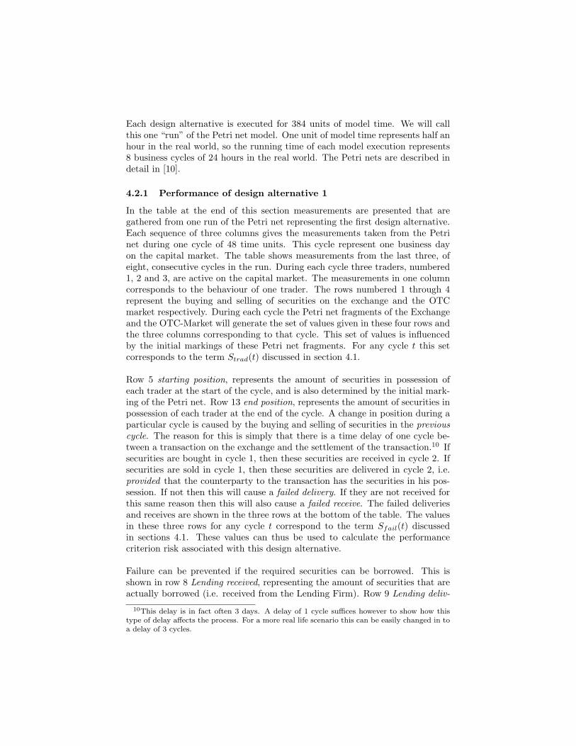
Each design alternative is executed for 384 units of model time. We will callthis one “run” of the Petri net model. One unit of model time represents half anhour in the real world, so the running time of each model execution represents8 business cycles of 24 hours in the real world. The Petri nets are described indetail in [10].

4.2.1 Performance of design alternative 1

In the table at the end of this section measurements are presented that aregathered from one run of the Petri net representing the first design alternative.Each sequence of three columns gives the measurements taken from the Petrinet during one cycle of 48 time units. This cycle represent one business dayon the capital market. The table shows measurements from the last three, ofeight, consecutive cycles in the run. During each cycle three traders, numbered1, 2 and 3, are active on the capital market. The measurements in one columncorresponds to the behaviour of one trader. The rows numbered 1 through 4represent the buying and selling of securities on the exchange and the OTCmarket respectively. During each cycle the Petri net fragments of the Exchangeand the OTC-Market will generate the set of values given in these four rows andthe three columns corresponding to that cycle. This set of values is influencedby the initial markings of these Petri net fragments. For any cycle t this setcorresponds to the term Strad(t) discussed in section 4.1.

Row 5 starting position, represents the amount of securities in possession ofeach trader at the start of the cycle, and is also determined by the initial mark-ing of the Petri net. Row 13 end position, represents the amount of securities inpossession of each trader at the end of the cycle. A change in position during aparticular cycle is caused by the buying and selling of securities in the previouscycle. The reason for this is simply that there is a time delay of one cycle be-tween a transaction on the exchange and the settlement of the transaction.10 Ifsecurities are bought in cycle 1, then these securities are received in cycle 2. Ifsecurities are sold in cycle 1, then these securities are delivered in cycle 2, i.e.provided that the counterparty to the transaction has the securities in his pos-session. If not then this will cause a failed delivery. If they are not received forthis same reason then this will also cause a failed receive. The failed deliveriesand receives are shown in the three rows at the bottom of the table. The valuesin these three rows for any cycle t correspond to the term Sfail(t) discussedin sections 4.1. These values can thus be used to calculate the performancecriterion risk associated with this design alternative.

Failure can be prevented if the required securities can be borrowed. This isshown in row 8 Lending received, representing the amount of securities that areactually borrowed (i.e. received from the Lending Firm). Row 9 Lending deliv-

10This delay is in fact often 3 days. A delay of 1 cycle suffices however to show how thistype of delay affects the process. For a more real life scenario this can be easily changed in toa delay of 3 cycles.

ered, represents the amount of securities that is lent out (i.e. delivered to theLending Firm). These two figures must add up to zero because borrowing andlending does not change the amount of securities in the system. The deliveryof securities to the CCP is represented by row 10 Exch. deliv.. It might occurthat securities are bought on the OTC market and sold on the exchange in thesame cycle. If the securities that are bought on the OTC market are receivedafter the moment that delivery of the securities sold on the exchange to theCCP should occur, then this delivery will fail. If they are received before thatmoment then the delivery will succeed. This issue plays a critical role in thedifference between the design alternatives discussed in section 2.2. Row 6 is re-served for securities that have been bought on the OTC-Market and have beenreceived in time to be used for delivery to the CMF and CCP. Row 11 is forthose that have been received too late.

As explained in section 2.2 the point in time that securities bought on theOTC market are received is crucial in the relative performance of the two de-signs alternatives. The measurements are taken under the assumption that thesecurities bought on the OTC market are received just one time unit beforedelivery of securities to the CCP occurs, referred to in sections 2 and 2.2 phaseD2, but after phase D1. The timing of phase D2 is fixed by the CCP and is thesame in both design alternatives. The measurements show that, under theseassumptions, in the first design alternative the delivery of these securities willsucceed, they show up in row 6. In the next section it is shown that the deliveryof these securities in the second design alternative will not succeed, they willthen show up in row 11.

Cycle T=6 T=7 T=8Trader 1 2 3 1 2 3 1 2 31 Exch. bought - - 15 - - 15 - - 152 Exch. sold 27 72 - 27 72 - 27 72 -3 OTC bought - 30 - - 30 - - 30 -4 OTC sold 9 - 22 18 - 11 9 - 225 Start position 64 0 0 0 0 10 0 0 06 OTC received - - - - 30 - - 30 -7 Exch. received - - 15 - - 15 - - 158 Lending received - 42 - 18 7 - 5 10 -9 Lending deliv. 37 - 5 - - 25 - - 1510 Exch. deliv. 27 72 - 18 37 - 5 40 -11 OTC received - - - - - - - - -12 OTC delivered - - - - - - - - -13 End position 0 0 10 0 0 0 0 0 014 OTC failed deliv. 18 - 11 9 - 22 18 - 1115 Exch. failed deliv. - - - 9 35 - 31 67 -16 Exch. failed receives - - - - - - - - -

4.2.2 Performance of design alternative 2

The table below shows measurements taken from one run of the Petri net rep-resenting the second design alternative. It shows clearly that the performanceis worse. First of all the number of failed settlements, shown in the 3 rows atthe bottom of each table, is higher. This means that the level of risk in thesecond design alternative is higher. Secondly more borrowing is necessary inthe second design alternative compared to the first. This can be seen from themeasurements shown in rows 8 and 9. This means that the borrowing costs inthe second design alternative are higher than in the first and thus the efficiencyof the Clearing and settlement process in second design alternative is lower thanin the first. The level of settlement cost in the second design alternative is alsohigher. This can not be seen directly from this table, because it doesn’t containa count of the number of settlement instructions. It can be inferred howeverby looking at the values in row ten, “Exch. deliv.”. The sum of the entries inthis row corresponds to the total number of securities that have been deliveredby the CMF to the CCP. In the table with measurements of the second designalternative this sum is lower than in the table with measurements of the firstdesign alternative. In each cycle there is only one instruction sent from the CMFto the CCP. So this means that per instruction less securities are delivered inthe second design alternative, and the cost per security delivered is thus higher.This is of course a logical consequence of the fact that there are more settlementfailures in the second design alternative.

Cycle T=6 T=7 T=8Trader 1 2 3 1 2 3 1 2 3Exchange bought - - 15 - - 15 - - 15Exchange sold 27 72 - 27 72 - 27 72 -OTC bought - 30 - - 30 - - 30 -OTC sold 9 - 22 18 - 11 9 - 22Start position 9 30 25 0 30 7 0 30 0OTC received - - - - - - - - -Exchange received - - 0 - - 0 - - 0Lending received - 18 - - 7 - - - -Lending deliv. - - 18 - - 7 - - -Exchange deliv. 9 48 - 0 37 - 0 30 -OTC received - 30 - - 30 - - 30 -OTC deliv. - - - - - - - - -End position 0 30 7 0 30 0 0 30 0OTC failed deliv. 18 - 11 9 - 22 18 - 11Exchange failed deliv. 18 24 - 45 59 - 72 101 -Exchange failed receives - - 15 - - 30 - - 45

5 Concluding remarks

In this final section the research questions posed in section 1 will be discussedin the light of the experience gained by the case study. Also some issues will beraised concerning the use of CPN-Tools.

Are HTCPNs suitable for modelling the Clearing and settlement process?The case study illustrates that HTCPNs have sufficient expressiveness to modelthe relevant characteristics of the Clearing and settlement process. These char-acteristics can be categorized as follows:

1. Decentralized control

2. High complexity

3. Time critical

Decentralized control The Clearing and settlement process involves a largenumber of different participants, like the traders, Clearing Member Firms, Cus-todians, Lending Firms, the CCP, and the CSD, that have been described inthis paper. Each of these participants in general only controls a part of theprocess and independently decides about the course of action to be taken. Theconsequence however is that the performance of the Clearing and settlementprocess as a whole, measured by the criteria described in section 4.1, dependsvery much on efficient cooperation between the participants. Petri nets are wellsuited to model both independence and cooperation.

High complexity It requires several hundreds of places and transitions tomodel the Clearing and settlement process [10]. The primary page located atthe top of the hierarchy of the HTCPNs, shown in section 3, represent theClearing and settlement process with only 7 transitions and several tenths ofplaces. Without a hierarchy concept it would be difficult to develop these mod-els in a controlled way. It allowed to translate high level concepts like “CSD”,Custodian, “CMF” etc. familiar to business experts directly into substitutiontransitions. The use of coloured tokens also reduced the complexity of the Petrinet models. For instance, concepts such as trades, settlement instructions oraccounts are translated into structured coloursets which would be hard to modelin a PT-net.

Time critical The performance criteria described in section 4.1 imply thattiming is an important determinant of the performance of the clearing andsettlement process. The HTCPN allowed to model the timing aspect of theClearing and settlement process satisfactorily by attaching time-stamps to to-kens and delay statements to the arcs or transitions.

The following issues concerning the use of CPN Tools can be raised. Firstlypriorities between transitions is modelled in figure 5 by using time stamps. Per-haps other ways of doing this might be more appropriate. Secondly, moving

around of highly structured data, typical for this kind of applications, is some-times a bit inconvenient. To name a small example: if a highly structuredoutput token is created from an input token which is the same except for onesmall item in the token, all items must be copied explicitly resulting is relativelylong lines of code. Furthermore, applications like the one explored in this casestudy might benefit from more tool support for the modelling of data.

Are HTCPNs helpful in validating process models?Because the transitions and most of the places on the primary pages of the Petrinets can be mapped to familiar business concepts, the graphical representationof these primary pages could be easily explained to business experts. The vali-dation of the dynamics of the Petri net was performed by showing an animationof the Petri net. This appeared to be a bit more tricky. The following issuescan be raised concerning the animation of behaviour with CPN-Tools:Firstly, animation by CPN-Tools shows a snap shot of the entire net and statespace after each step (or sequence of steps). No distinction is made between thepart of the state space that has changed and the part that hasn’t change. Ifthe net is large enough it is difficult to see for an observer what has happenedbetween two snapshots. Secondly it is difficult for a human observer to get apicture of the entire occurrence sequence. To do that he has to remember all thesnapshots he has seen. Thirdly, dynamics of transitions in a HTCPN is definedby the Petri nets on the underlying subpages. But validation of the entire Petrinet model by a process owner or business expert is preferably done by animat-ing the net on the primary pages, because that is the level he understands thebest. Fourthly the squares and circles used by CPN-Tools to represent activ-ities and communication are slightly alien to business experts. More domainspecific symbols might do better. Finally the tables with performance mea-surements gathered during the animation described in section 4.2 also provedhelpful in explaining the behaviour of the net. This type of reporting is oftenquite familiar to process owners and business experts. Creating these reportswas somewhat time consuming. Creating support in CPN-Tools to address theissues just mentioned might ease the process of model validation.

Can HTCPNs effectively be used to decide between design alternatives?Performance analysis of the design alternatives for the Clearing and settlementprocess by executing the Petri net models representing these design alternativesshowed better performance for the first design alternative relative to the second,as was expected. This might seem a bit trivial, because this result just confirmsthe informal explanation of the difference between the two design alternativesgiven in section 2.2. In reality this difference became only clear after the modelswere built and compared by means of model execution. The informal explana-tion is historically of later date than the results of model execution. In factthe development of the Petri net models was an iterative process, going backand forth between model building and model execution on the one hand andinformal conception of what was going on on the other. This shows that formalmodel building and model execution are useful tools to create insight and under-standing of a process design and its performance. Some additional tool support

for creating model variants might however be convenient. Large fragments ofboth design alternatives (i.c. what is designated as “market infrastructure”,i.e. CSD, CCP, Exchange and OTC-market) are the same. In the case studypresented here, the Petri net model of the market infrastructure representingthe first design alternative was copied into the Petri net model representing thesecond design alternative. This has obvious drawbacks. Having just one copywould be better.

References

[1] W. van der Aalst; Timed coloured Petri nets and their application to logis-tics, Phd thesis Tue, 1992

[2] Clearnet; Introduction of Clearing 21 for the clearing of cash products(phase 2) in the Amsterdam branch of Clearnet, Aug. 2002

[3] Clearnet; Main specifications for the migration from Cash Dutch applica-tions towards Clearing21 Version 1.2, 16 May. 2002

[4] LCH Clearnet; Settlement Connect - Detailed specifications of Clearing 21Version 5, Feb. 2004

[5] Euroclear Nederland; Euroclear Nederland Guidelines, Amsterdam, 27 oc-tober 2005

[6] The Giovannini Group; Cross-Border Clearing and Settlement Arrange-ments in the European Union, Brussels, 2001

[7] K. Jensen; Coloured Petri Nets; Basic Concepts, Analysis Methods andPractical Use; Vol. 1, Springer-Verlag, 1992

[8] K. Jensen; Coloured Petri Nets; Basic Concepts, Analysis Methods andPractical Use; Vol. 2, Springer-Verlag, 1995

[9] M. Kohn; Financial Institutions and Markets, Oxford University Press,2004

[10] P. M. Kwantes; Design of Clearing and settlement operations: a case studyin Business Process Modelling and Analysis with Petri nets, Masters Thesis,Leiden Unniversity, 2006

[11] T. H. Mclnish; Capital Markets, A Global Perspective, Blackwell PublishersInc., 2000

Some Rules to Transform Sequence Diagrams

into Coloured Petri Nets ⋆

Oscar R. Ribeiro and Joao M. Fernandes

{oscar.rafael, jmf}@di.uminho.ptDept. of Informatics, University of Minho, Portugal

Abstract. This paper presents a set of rules that allows software engi-neers to transform the behavior described by a UML 2.0 Sequence Dia-gram (SD) into a Colored Petri Net (CPN). SDs in UML 2.0 are muchricher than in UML 1.x, namely by allowing several traces to be com-bined in a unique diagram, using high-level operators over interactions.The main purpose of the transformation is to allow the developmentteam to construct animations based on the CPN that can be shown tothe users or the clients in order to reproduce the expected scenarios andthus validate them. Thus, non-technical stakeholders are able to discussand validate the captured requirements. The usage of animation is animportant topic in this context, since it permits the user to discuss thesystem behavior using the problem domain language. A small control ap-plication from industry is used to show the applicability of the suggestedrules.

1 Introduction

Although complex systems are, by their nature, hard to build, the problem canbe ameliorated if the user requirements are rigorously and completely captured.This task is usually very difficult to complete, since clients and developers donot use the same vocabulary to discuss. For behavior-intensive applications,this implies that the dynamic behavior is the most critical aspect to take intoaccount. This contrasts with database systems, for example, where the relationamong data types is the most important concern to consider. A scenario is aspecific sequence of actions that illustrates behaviors, starting from a well definedsystem configuration and in response to external stimulus. Petri nets are used toformalize the behavior of some component, system or application, namely thosethat have a complex behavior. Since Petri nets are a formal model, they do notcarry any ambiguity and are thus able to be validated.

This paper proposes a set of rules that allow software engineers to transformrequirements, expressed as a UML 2.0 SD into an behaviorally equivalent CPN.The main purpose of the transformation is to generate a CPN [1] that is akinto be animated (with the mechanism available in CPN-Tools) and thus under-stood by the users. The synthesized CPN that can be shown (i.e. animated) to

⋆ This work has been supported by the grant with reference SFRH/BD/19718/2004 from“Fundacao para a Ciencia e Tecnologia”

the users or the clients in order to reproduce the expected scenarios and thusvalidate them. Thus, non-technical stakeholders are able to discuss and validatethe captured requirements. The usage of animation is an important topic inthis context, since it permits the user to discuss the system behavior using theproblem domain language, which they are supposedly familiar with.

The paper is organized as follows. In section 2, the SDs of UML 2.0 are intro-duced. Section 3 presents some rules of how to translate a SD into a behaviorallyequivalent CPN. In section 4, the result of applying the rules presented in pre-vious section to the case study of an industrial reactor system. In Section 5 ispresented a discussion of the related work. Section 6 presents the conclusions ofthis work and some possible directions for the future work.

2 UML Diagrams for interaction

The introduction of UML 2.0 standard changed almost every sort of things inprevious versions designated by UML 1.0.

The dynamic part of the system can be specified in UML 2.0 through variousbehavioral diagrams, such as: activity diagrams, sequence diagrams and statemachines diagrams. These diagrams use behavioral constructs, namely activities,interactions, and state machines.

Interactions are a mechanism for describing systems, which can be under-stood and produced, at varying level of detail. Usually, interactions do not tellthe complete story, when they are produced by designers or by computer systems,because normally some other legal and possible traces are not contained withinthe described interactions. There are some exceptions where the project requestthat all possible traces of a system shall be documented through interactions.

An interaction is formed by lifelines and messages between them, that se-quence is important to understand the situation. Although data may be alsoimportant, its manipulation is not the focus of interactions. Data is carried bythe messages, and stored in the lifelines, and can be used to decorate the dia-grams.

SDs are the most common interaction diagram defined by the UML [2], thatfocus on the message interchange between a number of lifelines. Communicationdiagrams show interactions through an architectural view where the arcs be-tween the communicating lifelines are decorated with description of the passedmessages and their sequencing. Interaction overview diagrams are a variant ofactivity diagrams that define interactions in a way that promotes overview of thecontrol flow, these diagrams can be seen as a high-level structuring mechanismthat is used to compose scenarios through sequence, iteration, concurrency orchoice. There are also optional diagram notations such as timing diagrams andinteraction tables. In this work, we concentrate on SDs.

In the UML 2.0 new notions for SDs are introduced to treat iterative, con-ditional and various other control of behavior. The old iteration markers andguards on messages have been dropped from SDs.

Fig. 1: An example of a UML 2.0 SD

Fig. 1 shows an example of a SD. A SD is enclosed in a frame and includesa pentagon in the upper left handed corner with the keyword sd followed by alabel identifying the SD.

There are several possible operators, whose meaning is described informallyin the UML 2.0 Superstructure specifications [2]:

– sd: Indicates the principal frame of the sequence diagram;– ref: references another fragment of interaction;– seq: indicates the weak sequencing of the operands in the fragment, which

is select by default. The weak sequencing maintain the order inside eachoperand, and the events on different operands and different lifelines mayoccur in any order.

– strict: specifies that messages in the fragment are fully ordered;– alt: specifies that the fragment represents a choice between two possible

behaviors. There is a guard associated with the fragment, its evaluationdefine which of choices is executed;

– par: indicates that the fragment represents a parallel merge between thebehaviors of the operands;

– loop: indicates an interaction fragment that shall be repeated some numberof times. This may be indicated using a guard condition, and it is executeduntil the guard evaluates to false.

UML 2.0 provides two kinds of conditions in SDs, namely interaction con-

straints and state invariants. An interaction constraint is a boolean expressionshown in square brackets covering the lifeline where the first event will occur,positioned above that event inside an interaction operand. A state invariant is

a constraint on the state of an instance, and is assumed to be evaluated duringrun time immediately prior to the execution of the next event occurrence. No-tationally, state invariants are shown as a constraint inside a state symbol or incurly brackets, and are placed on a lifeline.

In the previous versions of UML it was not possible to express that, at anytime, a specific scenario should not occur. In the UML 2.0 negative behavior (i.e. invalid traces) can be specified using the new operator neg. Currently, thisoperator is not considered in this work.

3 Transforming SD Operators into CPNs

In this section we show how to translate some of the high-level operators availablein the UML 2.0 SDs, into a behaviorally equivalent CPN. To accomplish this, weexplain the semantics of the operator, we describe in an informal way how thetransformation is achieved, and additionally we show the result of applying theseideas to some illustrative examples. We restrict our study to the following high-level operators: strict, seq, par, loop and alt. Operators like neg, assert,critical are not considered by now.

First of all we look to InteractionFragments without any of the high-leveloperators. An InteractionFragment is a set of Lifelines, each of which has asequence of EventOccurences associated with it.

We consider a semantic for SD with a order relation between messages suchthat the emission requires the reception of the preceding message.

(a) A UML 2.0 SD without high-level oper-ators

()

()

()

m3(aB)

aB

()

m1(aB)

aB

()

()aC

m2(aC)

m3

m1

m2

UNIT

Fusion 2

B

UNIT

UNIT

Fusion 2 B

Fusion 3C

UNIT

Fusion 3

Fusion 2

Fusion 2

(b) The obtained CPN

Fig. 2: Example of transform a SD without high-level operators

The SD presented in Fig. 2a represents an interaction without high-leveloperators. There are three Lifelines and three messages between them. The ob-tained CPN (see Fig. 2b) associates a transition for each message in the SD. In

this way an execution of a message is represented by the firing of its correspond-ing transition in the CPN. There are places to guarantee the order between thefirring of transitions, and other places to represent the object which the messagechanges when executing. When firing a transition, a function is applied to theobject in the place. This function is a representation of the changes made in theobject of the lifeline in the message’s destination. To represent the guards in theSD we use a transition guarded by a conditions over the object representation.When there are more than one message in the same point of a lifeline we considera unique transition which includes all the messages.

Let us consider CombinedFragments with high-level operators.

3.1 Alternative Choice

The choice of behavior is represented by a CombinedFragment with the interac-

tionOperator alt. Each operand of alt has an associated guard, which is evalu-ated when choosing the operand to be executed. No more than one operand willbe chosen and in this work we assume that the guards must be disjoint. Whenone of the operands has its guard evaluated to true, the interaction associatedwith this operand is considered. The empty guard is by default evaluated totrue. The operand guarded by else means that the guard is evaluated to truewhen none of the guards in the other operands is evaluated to true. In the casethat none of the operands’ guards are evaluated to true (this means that thereare no else and empty guards) none of the operands are executed.

The SD in Fig. 3a is transformed into the CPN in Fig. 3b. Each operandin SD is transformed in a sequential branch. All sequential branchs begin in acommon input place and end a common output place.

(a) A UML 2.0 SD

()

anA anA

m3(aB)

aB

()

()

()

aC

m2(aC)

m1(aB)

()

()

()

aB ()

()

anA

()()()

m3

m2

m1

alt ELSEalt2

[cond2(anA)]

alt1

[cond1(anA)]

Fusion 1A

Fusion 1A

Fusion 2B

UNIT

UNIT

UNIT

UNIT

Fusion 3C

Fusion 2

B

Fusion 1A

UNIT

Fusion 1

Fusion 2

Fusion 3

Fusion 2

Fusion 1 Fusion 1

[(not (cond1 anA)) andalso (not (cond2 anA))]


Fig. 3: Example with the alternative choice operator (alt)

Please notice that in this case there is no else guard, and thus when none ofthe guards is evaluated as true, no operand is executed. In terms of CPNs this isrepresented by the rightmost part of the CPN where the “alt ELSE” transitioncondition is the negated disjunction of all other guards. The other branches areguarded by the same condition as in SD and describe the same sequence.

3.2 Optional

The optional operator, represented by InteractionOperator opt, can be seen asan alternative choice with only one Operand, whose guard is not the else (seeFig. 4). With this similarity, we can apply to the optional operator the samegeneral translation scheme used for alternative choice.

(a) A UML 2.0 SD (b) The corresponding UML 2.0 SD with alt

Fig. 4: The option operator (opt) expressed by an alternative choice

3.3 Parallel Composition

The parallel merge between two or more behaviours is represented by a Com-

binedFragment with the interactionOperator par. Keeping the order imposedwithin operands, EventOccurrences from different operands can be interleavedin any way. The SD in Fig. 5a is transformed into the CPN in Fig. 5b. Theobtained CPN has two additional transitions to control the interleaving of be-haviors. The transition “begin par” creates two branches (one for each operand)introducing a token into the two output places, in this way we obtain the inter-leaving between the transitions of each branch. The transition “end par” waitfor the execution of all created branches, because it is enabled only when itsinput place has a number of token equal to the number of created branches.

3.4 Weak Sequencing

When using the InteractionOperator seq the corresponding CombinedFragment

represents a weak sequencing between the behaviors of the operands. The or-

(a) A UML 2.0 SD

()

()

()

()

()

m3(aB)

aB

()

2`()

()

m1(aB)

aB

()

()

()

aC

m2(aC)

m3

end par

begin par

m1

m2

UNIT

Fusion 2 B

UNIT

UNIT

UNIT

Fusion 2 B

UNIT

UNIT

Fusion 3C

Fusion 3

Fusion 2 Fusion 2


Fig. 5: Example with the parallel composition operator (par)

dering of EventOccurrences within each of the operands are maintained in theresult. OccurrenceSpecifications on different lifelines from different operands maycome in any order. OccurrenceSpecifications on the same lifeline from differentoperands are ordered such that an EventOccurrence of the first operand comesbefore that in the second operand.

In Fig. 6a we have an example of a SD with seq operator. The messages m1and m3 have the EventOccurence in the same Lifeline, and in the first operand,after the message m1 we have the message m2. Thus, message m1 must occurbefore messages m3 and m2.

To construct a corresponding CPN to a SD with the seq operator, we firstconsider the CPN for the parallel composition between the operands, and afterthat we impose some more order between transitions in different branches. TheCPN in Fig. 6b is obtained from the CPN in Fig 5b changing the name of tran-sitions “begin par” and “end par”) to “begin seq” and “end seq”, adding theplace between transitions “m1” and “m3” and the corresponding arcs to completethe connection.

The SD in Fig. 7a is another example using the operator seq. The corre-sponding CPN is presented in Fig. 7b.

There are some particular cases using this operator. If the EventOccurrence ofthe last message from the first operand is in the same Lifeline as the first messageof the second operand, we have a sequential order between all the messages inthe operands. If none EventOccurrence of messages is in the same lifeline wehave a parallel composition between the operands.

(a) A UML 2.0 SD

()

()

2`()

()

()aC

m2(aC)

m3(aB)()

()

()

()

()

m1(aB)

aB

()

end seq

m2

m3

beginseq

m1

UNIT

Fusion 3C

UNIT

Fusion 2 B

UNIT

UNIT

UNIT

Fusion 2 B

UNIT

Fusion 2 Fusion 2

Fusion 3

UNIT

()

aB()


Fig. 6: Example with the weak sequencing operator (seq)

(a) A UML 2.0 SD

()m3(aB)

()

m2(aC)

aC

()()

()

()

()

()

()

2`()

()

()

m1(aB)

aB

()

()aC

m2(aC)

m3

m4

beginseq

end seq

m1

m2

Fusion 3C

UNIT

UNIT

UNIT

UNIT

Fusion 2 B

UNIT

UNIT

UNIT

Fusion 2 B

UNIT

Fusion 3C

Fusion 3

Fusion 2 Fusion 2

Fusion 3

() aB

UNIT

()

()


Fig. 7: Another example with the weak sequencing operator (seq)

3.5 Looping

The loop InteractionOperator represents the iterative application of the operandin the CombinedFragment. This iterative application can be controlled by a guardor by a minimum and maximum number of iterations.

Given the CPN for the operand inside the loop, we add two transitions:“loop” and “end loop”. These two transitions have the same input place. Tran-sition “loop” is enabled if the condition (guard for loop operator) evaluates totrue, and its output place is the input place for the operand’s CPN. The transi-tion “end loop” is enabled when the condition evaluates to false and its outputplace is used as connection to the end of the loop operator. In Fig. 8 we havean example with the loop operator.

(a) A UML 2.0 SD

aBaB

()

()

()()

m1(aB)

aB

()

()

()

()

aC

m2(aC)

[not (cond aB)][cond(aB)]

m1

Fusion 2B

Fusion 2B

UNIT

UNIT

Fusion 2B

UNIT

UNIT

Fusion 3C

Fusion 3

Fusion 2

Fusion 2 Fusion 2

m2

loop end loop


Fig. 8: Example with the looping operator (loop)

4 Validation of the Rules

To validate the proposed transformation rules we plan to apply them to severalcase studies, so that we can also evaluate their practical usefulness. Currently weare using an industrial reactor as a case study. In this chapter we show two CPNsfor the reactor: one obtained directly from the requirements (or more preciselyadapted from a PN-based specification) and another one obtained from a SDusing the proposed translation rules.

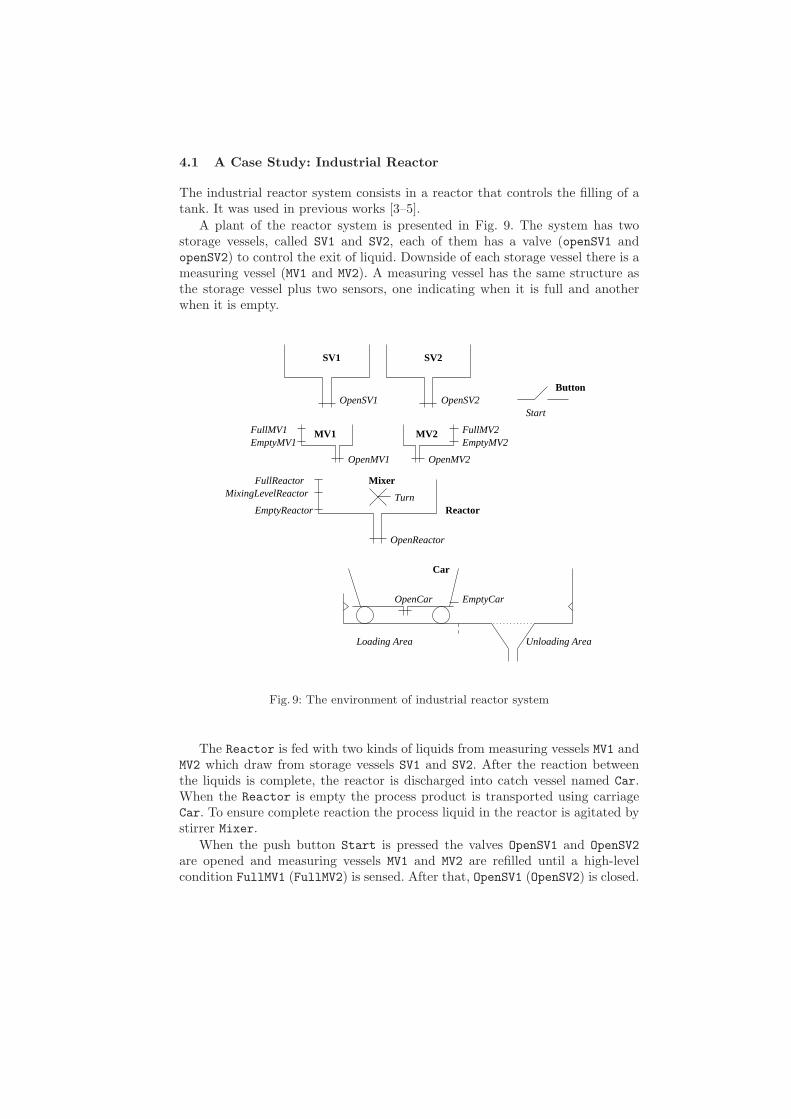
4.1 A Case Study: Industrial Reactor

The industrial reactor system consists in a reactor that controls the filling of atank. It was used in previous works [3–5].

A plant of the reactor system is presented in Fig. 9. The system has twostorage vessels, called SV1 and SV2, each of them has a valve (openSV1 andopenSV2) to control the exit of liquid. Downside of each storage vessel there is ameasuring vessel (MV1 and MV2). A measuring vessel has the same structure asthe storage vessel plus two sensors, one indicating when it is full and anotherwhen it is empty.

Start

OpenCar EmptyCar

Unloading AreaLoading Area

Car

OpenReactor

EmptyReactor Reactor

Mixer

Turn

MV2MV1EmptyMV1FullMV1

EmptyMV2FullMV2

OpenMV2OpenMV1

Button

SV2SV1

OpenSV1 OpenSV2

FullReactorMixingLevelReactor

Fig. 9: The environment of industrial reactor system

The Reactor is fed with two kinds of liquids from measuring vessels MV1 andMV2 which draw from storage vessels SV1 and SV2. After the reaction betweenthe liquids is complete, the reactor is discharged into catch vessel named Car.When the Reactor is empty the process product is transported using carriageCar. To ensure complete reaction the process liquid in the reactor is agitated bystirrer Mixer.

When the push button Start is pressed the valves OpenSV1 and OpenSV2

are opened and measuring vessels MV1 and MV2 are refilled until a high-levelcondition FullMV1 (FullMV2) is sensed. After that, OpenSV1 (OpenSV2) is closed.

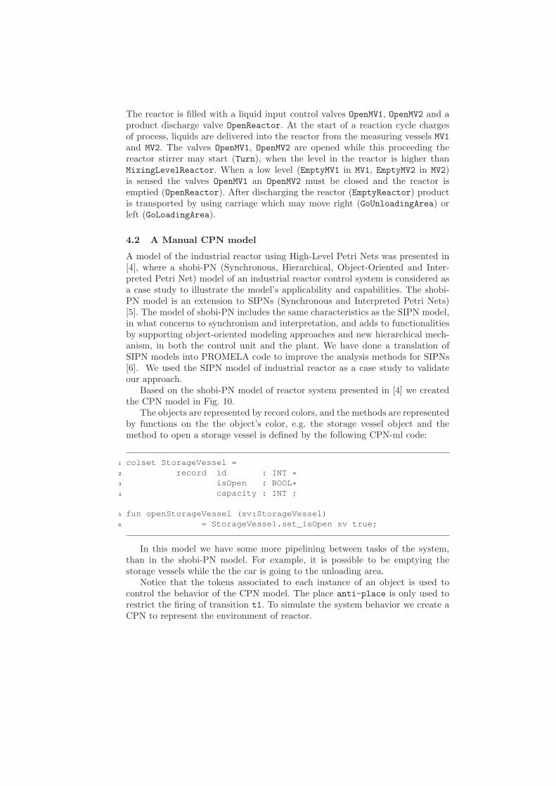
The reactor is filled with a liquid input control valves OpenMV1, OpenMV2 and aproduct discharge valve OpenReactor. At the start of a reaction cycle chargesof process, liquids are delivered into the reactor from the measuring vessels MV1and MV2. The valves OpenMV1, OpenMV2 are opened while this proceeding thereactor stirrer may start (Turn), when the level in the reactor is higher thanMixingLevelReactor. When a low level (EmptyMV1 in MV1, EmptyMV2 in MV2)is sensed the valves OpenMV1 an OpenMV2 must be closed and the reactor isemptied (OpenReactor). After discharging the reactor (EmptyReactor) productis transported by using carriage which may move right (GoUnloadingArea) orleft (GoLoadingArea).

4.2 A Manual CPN model

A model of the industrial reactor using High-Level Petri Nets was presented in[4], where a shobi-PN (Synchronous, Hierarchical, Object-Oriented and Inter-preted Petri Net) model of an industrial reactor control system is considered asa case study to illustrate the model’s applicability and capabilities. The shobi-PN model is an extension to SIPNs (Synchronous and Interpreted Petri Nets)[5]. The model of shobi-PN includes the same characteristics as the SIPN model,in what concerns to synchronism and interpretation, and adds to functionalitiesby supporting object-oriented modeling approaches and new hierarchical mech-anism, in both the control unit and the plant. We have done a translation ofSIPN models into PROMELA code to improve the analysis methods for SIPNs[6]. We used the SIPN model of industrial reactor as a case study to validateour approach.

Based on the shobi-PN model of reactor system presented in [4] we createdthe CPN model in Fig. 10.

The objects are represented by record colors, and the methods are representedby functions on the the object’s color, e.g. the storage vessel object and themethod to open a storage vessel is defined by the following CPN-ml code:

1 colset StorageVessel =2 record id : INT *3 isOpen : BOOL*4 capacity : INT ;

5 fun openStorageVessel (sv:StorageVessel)6 = StorageVessel.set_isOpen sv true;

In this model we have some more pipelining between tasks of the system,than in the shobi-PN model. For example, it is possible to be emptying thestorage vessels while the the car is going to the unloading area.

Notice that the tokens associated to each instance of an object is used tocontrol the behavior of the CPN model. The place anti-place is only used torestrict the firing of transition t1. To simulate the system behavior we create aCPN to represent the environment of reactor.

e

e

aCar

goLoadingArea(aCar)

aReactor

aReactorturnOffMixer(aMixer)

(aReactor,aMixer)

aCar

aCar

goUnloadingArea(aCar)

aCar

aCar

openCar(aCar)

(openReactor(aReactor),aMixer)

(aReactor,aMixer) aCar

listEmptyMVs

aMV

aMV(aReactor, turnOnMixer(aMixer))

aReactor

closeAllMVs(listEmptyMVs)

closeReactor(aReactor)

openAllMVs(listFullMVs)aReactor

aReactorlistFullMVs

closeCar(aCar)

aCar

aCaraMV

aMV

closeSV(aSV)

aSV

openAllSVs

aButton

listStorageVessels

t1b

t10b

[isAboveMixingLevelReactor(aReactor)]

t13

[isEmptyCar(aCar)]

t12

[isAtUnloadingArea(aCar)]

t11

[isEmptyReactor(aReactor)]

t10

t7 t8

[isEmptyMV(aMV)]

t5

[isAtMixingLevelReactor(aReactor)]

t4 t9

[isAtLoadingArea(aCar)]

t2 t3

[isConnected(aSV,aMV) andalso isFullMV(aMV)]

t1

[isPressed(aButton)]

anti-place

1`e

E

p14c

Fusion 4

Reactor

p14b

Car

p16

Car Events 3

Car

p15

Car Events 2

Car

p14

Fusion 3

Reactor_x_Mixer

p13

Car

p11 p12

MeasuringVessel

p7

Reactor_x_Mixer

mixer

Mixer

p9 10

MV Events2 MeasuringVessel

p8

Fusion 2Reactor

pf8

reactor

Reactor

p4 p5

MeasuringVessel

pf6 7

MV Events1

listMeasuringVessels

MeasuringVessel

p2 p3

SV EventsStorageVessel

p6Car Events 1

Car

Pf4

listCars

Car

Pf2

Fusion 1

1`false

ButtonPf 1 2

listStorageVessels

StorageVessel

Fusion 1

Car Events 1SV Events

MV Events1

Fusion 2

MV Events2

Fusion 3

Car Events 2

Car Events 3

Fusion 4

aMixer

Fig. 10: A CPN model for reactor system

4.3 A CPN model from a SD

This subsection presents a SD for some scenarios of reactor system’s usage, anda CPN model obtained from the SD through the rules presented in section 3.

The reactor system is textually described in subsection 4.1, and in subsection4.2 there is a CPN model which defines its behavior. Taking into account thesetwo exercises of analyzing the reactor system we construct the SD in Fig. 11 torepresent the handled scenarios. This SD uses high-level operators, namely theref to point to another two SDs: “Preparing Car” (see Fig. 12) and “VesselsBehavior” (see Fig. 13).

Fig. 11: A SD describing some scenarios of using the reactor system

To transform this SD we firstly apply the rules to the fragments with onehigh-level operator. After that we compose the obtained CPNs into a hierarchicalCPN. We put each SD pointed by ref into a subpage. Fig. 14 shows the CPNobtained from the SD in Fig. 12, where we can find transitions which are linksto a CPN in a subpage. The subpage Vessels Behavior is presented in Fig. 14,which corresponds to the SD presented in Fig. 12.

Fig. 12: A SD describing the behavior of vessels

Fig. 13: A SD describing the preparation of car

openReactor(aReactor)

aReactor

closeMVs(listAllMVs)

listAllMVs

start(aButton)

aButton

aButtonaButton

()

()

()

()

()

()

2`()

()

()()()

()

()

()

()

()

()

()()

()

()

2`()

()

()

()

()

()

()

Preparing Car_

Prepapring Car

end par 2

begin par 2

CloseAllMVsopenReactor

Preparing Car

Prepapring Car

VesselsBehavior

Vessels Behavior

Transport

Transport

VesselsBehavior_

Vessels Behavior

end loop

[not (isPressed aButton)]

Start

loop

[isPressed(aButton)]

begin par 1

end par 1

Fusion 4Reactor

Fusion 3MeasuringVessel

Fusion 1Button

Fusion 1Button

Fusion 1Button

UNIT

UNITUNIT

UNIT

UNIT

UNIT

UNIT

1`()

UNIT

UNIT

UNIT

UNIT

UNIT

UNIT

Vessels BehaviorTransport

Vessels Behavior Prepapring Car

Prepapring Car

Fusion 1 Fusion 1

Fusion 1

Fusion 3

Fusion 4

Fig. 14: CPN from the SD presented in Fig. 11

()()

() ()

()

()()

()

()

()

()

()

()

()

()

()

2`()

()()

()

()

()

()

()

Start Emptying MVs

Start Emtying MVs

Mix

Mix

end par 2

begin par 2

openAllSVs

end par 1

begin par 1

closeSV2

Full MV2Full MV1

closeSV1

UNIT UNIT

UNITUNIT

UNIT

UNIT

UNIT

UNIT

UNITUNIT

UNIT

InUNIT

OutUNIT

Out

In

MixStart Emtying MVs

Fusion 2

listAllSV

StorageVessel

openSVs(listAllSV)

Fusion 2 Fusion 2StorageVessel

closeSV(sv1)

StorageVessel

sv2

closeSV(sv2)

Fusion 2

Fusion 2 Fusion 2

Fusion 3Fusion 3MeasuringVessel

mv1

sv1

mv2

[isFullMV mv2][isFullMV mv1]

Fusion 3

MeasuringVessel

Fusion 3

Fig. 15: CPN to represent the behavior of vessels (see Fig. 12)

4.4 Animation

We have developed a SceneBeans [7] animation to be associated with the createdCPNs, through the BRITNeY animation tool [8]. A screen shot of the animationof reactor system is shown in Fig. 16.

In this animation we can find the elements of the problem domain, which isthe reactor domain. We obtain this animation using the Scenebeans animator.On the left top side of the image we have commands accepted by the animation.On the left button side, we have the events produced by animation. These setof commands and events are use to do the interaction between the animationand the CPN models. For example, to animate the message “openAllSVs” inSD of Fig. 12, we invoke, in the corresponding transition, two commands of theanimation: “openSV1” and “openSV2”. The user can interact with the animationusing the start button. The vessels on the top are the storage vessels. Eachstorage vessel has a corresponding measuring vessel. In the center we have thereactor vessel, with a mixer inside of it. On the button we have which transportsthe liquid to the unloading area.

This animation is intended to help us in validating the obtained CPNs interms of their appropriateness to express in the user’s domain language the re-quirements of a given system. Additionally we plan to use the animation tocompare the two CPNs for the reactor system (Figs. 10 and 14) and to eval-uate the performance of the rules to generate “good” CPNs. We would like to

Fig. 16: The animation of the reactor system

observe if the animations controlled by both CPNs produce the same externallyobservable behavior, independently of their internal structures.

5 Related work

Transforming scenarios into state-based models (namely, sequential finite-statemachines) has been the subject of many researchers. In fact, several approacheswere already proposed to combine the usage of both scenarios and state-basedmodels and, in this section, some of them are discussed. A major problem forobtaining state-based models from scenarios is the big computational complexityof the synthesis algorithms that does not allow the technique to scale up. Someadditional obstacles include methodological issues, the definition of the level ofdetail in the scenarios to allow effective synthesis, to the problem of guaranteeingthat the scenarios are representative of the users’ intentions.

The majority of the approaches propose the usage of FSM (finite state ma-chine). Kruger et al. suggest the usage of Message Sequence Charts (MSCs)for scenario based specifications of component behavior, especially during therequirements capture phase of the software process [9]. They discuss how toschematically derive statecharts from MSCs, in order to have a seamless de-velopment process. Harel proposes the usage of scenario based programming,through UML (Unified Modeling Language) [2] use cases and play in scenar-ios [10]. Harel’s play in scenarios make it possible to go from a high level userfriendly requirements capture method, via a rich language for describing message

sequencing, to a full model of the system, and from there to the final implemen-tation.

Whittle and Schumann propose an algorithm to automatically generate UMLstatecharts from a set of UML sequence diagrams [11]. The usage of this algo-rithm for a real application is also presented [12, 13], and the main conclusionis that it is possible to generate code mostly in an automatic way from scenariobased specifications.

Hinchey et al. propose a round trip engineering approach, called R2D2C(Requirements to Design to Code), where designers write requirements as sce-narios in constrained (domain specific) natural language [14]. Other notationsare however also possible, including UML use cases. Based on the requirements,an equivalent formal model, using CSP, is derived, which is then used as a basisfor code generation.

Uchitel and Kramer present an MSC language with semantics in terms of la-beled transition systems and parallel composition [15]. The language integratesother languages based on the usage of high level MSCs and on the identificationof component states. With their language, scenario specifications can be brokenup into manageable parts using high level MCSs. These authors also presentan algorithm that translates scenarios into a specification in the form of Fi-nite Sequential Processes, which can be used for model checking and animationpurposes.

The synthesis of Petri nets from scenario-based specification is less popu-lar than the one that generates FSMs, because Petri nets represent a model ofcomputation, where parallelism and concurrency of activities are “natural” char-acteristics. We next describe some of the approaches proposed to obtain Petrinets from a set of scenarios. In [16], the authors present a polynomial algorithmto decide if a scenario, specified as a Labelled Partial Order, is executable in agiven place/transition Petri net. The algorithm preserves the given amount ofconcurrency and does not add causality. In case the scenario is indeed executablein the Petri net, the algorithm computes a process net that respects the concur-rency expressed by the scenario. Although quite useful, this technique is not yetavailable for high-level Petri nets, such as Object-oriented Petri nets, ColoredPetri nets (CPNs), or Reference nets.

In [17] an informal methodology to map Live Sequence Charts (LSCs) intoCPNs is presented, for allowing properties of the system to be verified and ana-lyzed.

The formal translation of Interaction Overview Diagrams (IODs) into PEPAnets is described in [18]. PEPA nets constitute a performance modeling languagethat consists of a restriction of Petri nets, where tokens are terms of a stochasticprocess algebra [19]. The translation is based on the idea that the structure givenby the IOD corresponds to the high level net structure of the PEPA net, andthe behavior described in the IOD nodes (sequence diagrams) can be translatedonto PEPA terms. The translation allows a designer to formally analyze UML2.0 models, using the tools for PEPA nets.

A formal semantics by means of Petri nets is presented in [20] for the major-ity of the concepts of sequence diagrams. This semantics allows the concurrentbehavior of the diagrams to be modeled and subsequently analyzed. Moreover,the usage of CPNs permits an efficient structure for data types and control el-ements. In their approach they use places to represent the messages, insteadtransitions as we do.

This work is based on the preliminary results presented in [21], where theauthors show how the behavior of animation prototypes results from the trans-lation of SDs into CPNs. We extend their results by showing how to translatemore types of operators in UML 2.0 SDs, namely by considering parallel con-structors which result in CPNs with true concurrency (i.e. CPNs that are notjust sequential machines).

6 Conclusions

In this paper we show a set of rules to transform SD into equivalent CPNs foranimation proposes. In UML 2.0, SDs are quite expressive and this work exploresthe new constructors (in relation to UML 1.x) that allow several plain sequencesto be combined in a unique SD. Thus the rules allow the generation of a CPNthat covers several sequences of behaviors. This work is in progress so we plan todevelop it further. First we plan to investigate all SD operators, namely the neg

operator and evaluate if it can be useful for the software engineer. Second, weneed to better tune the rules, to realize if they can be automated. In the futurewe would like to use a UML-based tool to draw the SD diagrams and apply au-tomatically the rules to obtain a CPN for animation. Probably this automationrequires a second set of rules that “optimizes” the CPN by eliminating redun-dant parts. In this work we only have a validation of transformations thoughthe implementation, we plan to study the soundness and completeness of theapproach.

Finally the usage of the rules in real-world projects is planned, since webelieve that methods and tools for software engineers need to be evaluated bythem in complex industrial projects.

References

1. Jensen, K.: Coloured Petri Nets. Basic Concepts, Analysis Methods and PracticalUse. Brauer, W. and Gozenberg, G. and Salomaa edn. Volume Volume 1, BasicConcepts of Monographs in Theoretical Computer Science. Springer-Verlag (1997)ISBN: 3-540-60943-1.

2. Fowler, M.: UML Distilled: A Brief Guide to the Standard Object ModellingLanguage. Addisson-Wesley (2003)

3. Adamski, M.: Direct Implementation of Petri Net Specification. In: 7th Interna-tional Conference on Control Systems and Computer Science. (1987) 74–85

4. Machado, R.J., Fernandes, J.M., Proenca, A.J.: Specification of Industrial DigitalControllers with Object-Oriented Petri Nets. In: IEEE International Symposiumon Industrial Electronics (ISIE’97). Volume 1. (1997) 78–83

5. Fernandes, J.M., Pina, A.M., Proenca, A.J.: Concurrent Execution of Petri Netsbased on Agents. In: Encontro Nacional do Colegio de Engenharia Electrotecnica(ENCEE95), Lisbon Portugal, Ordem dos Engenheiros (1995) 83–9

6. Ribeiro, O.R., Fernandes, J.M., Pinto, L.F.: Model Checking Embedded Systemswith PROMELA. In: 12th IEEE International Conference on the Engineering ofComputer Based Systems (ECBS 2005), Greenbelt, MD, E.U.A., IEEE ComputerSociety Press (2005) 378–85

7. Pryce, N., Magee, J.: SceneBeans: A Component-Based Animation Framework forJava. (Online) http://www-dse.doc.ic.ac.uk/Software/SceneBeans/.

8. Westergaard, M., Lassen, K.B.: Building and Deploying Visualizations of ColouredPetri Net Models Using BRITNeY Animation and CPN Tools. In: Sixth Workshopand Tutorial on Practical Use of Coloured Petri Nets and the CPN Tools. (2005)

9. Kruger, I., Grosu, R., Scholz, P., Broy, M.: From MSCs to Statecharts. In Rammig,F.J., ed.: Distributed and Parallel Embedded Systems, Kluwer Academic Publish-ers (1999) 61–71

10. Harel, D.: From play-in scenarios to code: An achievable dream. IEEE Computer34(1) (2001) 53–60 (Also, Proc. Fundamental Approaches to Software Engineering(FASE; invited paper), Lecture Notes in Computer Science, Vol. (Tom Maibaum,ed.), Springer-Verlag, March 2000, pp. 22-34.).

11. Whittle, J., Schumann, J.: Generating statechart designs from scenarios. In: 22ndInternational Conf. on Software (ICSE), Limerick, Ireland (2000) 314–323

12. Whittle, J., Saboo, J., Kwan, R.: From scenarios to code: An air traffic controlcase study. In: ICSE’03. (2003) 490–497

13. Whittle, J., Kwan, R., Saboo, J.: From scenarios to code: An air traffic controlcase study. Software and Systems Modeling 4(1) (2005) 71 – 93

14. Hinchey, M.G., Rash, J.L., Rouff, C.A.: A formal approach to requirements-basedprogramming. ecbs 00 (2005) 339–345

15. Uchitel, S., Kramer, J.: A workbench for synthesising behaviour models fromscenarios. In: Proceedings of the 23rd International Conference on Software Engi-neering, ICSE 2001, 12-19 May 2001, Toronto, Ontario, Canada, IEEE ComputerSociety (2001) 188–197

16. Juhs, G., Lorenz, R., Desel, J.: Can I Execute My Scenario in Your Net? InCiardo, G., Darondeau, P., eds.: Applications and Theory of Petri Nets 2005: 26thInternational Conference (ICATPN 2005). Volume 3536 of LNCS., Miami, USA,Springer (2005) 289

17. Amorim, L., Maciel, P., Nogueira, M., Barreto, R., Tavares, E.: A methodologyfor mapping live sequence chart to coloured petri net. In: IEEE InternationalConference on Systems, Man and Cybernetics. Volume 4. (2005) 2999–3004

18. Kloul, J., Kuster-Filipe, J.: From interaction overview diagrams to pepa nets.In: Proceedings of the 4th Workshop on Process Algebras and Timed Activities(PASTA’05), Edinburgh (2005)

19. Gilmore, S., Hillston, J., Kloul, L., Ribaudo, M.: Pepa nets: a structured perfor-mance modelling formalism. Performance Evaluation 54(2) (2003) 79–104

20. Eichner, C., Fleischhack, H., Meyer, R., Schrimpf, U., Stehno, C.: Compositionalsemantics for UML 2.0 sequence diagrams using Petri Nets. In Lecture Notes inComputer Science, Volume, J.., ed.: SDL 2005: Model Driven Systems Design: 12thInternational SDL Forum. Volume 3530., Grimstad, Norway (2005) 133–148

21. Machado, R.J., Lassen, K.B., Oliveira, S., Couto, M., Pinto, P.: Execution ofUML Models with CPN Tools for Workflow Requirements Validation. In: SixthWorkshop and Tutorial on Practical Use of Coloured Petri Nets and the CPNTools. (2005)

Inside LoLA - Experiences from building a state

space tool for place transition nets

Karsten WolfUniversitat Rostock

18051 Rostock, Germany

1 History of LoLA

The development of LoLA started in the second half of the 1990s when researchresults on symmetry reduction and partial order reduction needed to be vali-dated with the help of a prototype implementation. At that time, the authorworked with Peter Starke who developed the Petri net analysis tool INA. Itturned out that, due to unfortunate design decisions in the core part of INA,algorithms run in unacceptable time. Consequently, a new core part of a veri-fication tool was designed, based on the analysis of time consumption in INA.This core, step by step complemented with state space based verification tech-niques, was later on called LoLA and first presented at the Petri net conferencein 2000.

Meanwhile, LoLA is integrated in several tool platforms including CPN-AMIof Universite Paris VI, the Model Checking Kit of Universitat Stuttgart, and thePetri Net Kernel of Humboldt-Universitat zu Berlin. It was successfully usedin several case studies, including the detection of hazards of an asynchronouscircuit that is part of a globally asynchronous - locally synchronous chip designfor coding and decoding signal of a 802.11 WLAN protocol, the validation ofa Petri net semantics for the Business Process Execution Language for WebServices (BPEL), and for the verification of block-level distributed programs.LoLA was able to solve a challenge example posted some years ago by HubertGaravel. The example stemmed from a LOTOS specification. The verificationproblem was quasi-liveness.

2 Features of LoLA

LoLA can read place transition nets and high level nets in formats that areeasy to read, easy to write, and easy to generate. It can not yet read PNMLbut translate its own format into PNML code. Once started, LoLA calculatesa state space for the purpose of verifying a property on-the-fly. That is, LoLAstops execution as soon as the property to be verified is settled. The classof properties to be verified can be selected at compile-time, through editing a

particular file userconfig.H. In the same file, the reduction techniques to beused can be specified. Consequently, one can generate different executable files,each specialized on one particular property and one particular combination ofreduction techniques.

The classes of properties that can be verified using LoLA include

• Reachability of a marking or a state predicate,

• Liveness of a transition or a predicate,

• Reversibility and existence of home states of the net,

• Quasi-liveness (non-death) of a transition,

• Boundedness of a place or the net,

• Existence of deadlocks,

• Model checking for CTL,

• The linear time properties Fφ, GFφ, and FGφ.

The particular formula, predicate, place, or transition to be checked can beread from a separate file. For state space reduction, LoLA offers

• Partial order reduction, with optimized versions for the various properties,

• The symmetry method, including an automatic exploration of the sym-metries,

• The coverability graph technique,

• The sweep-line method, including an automatic generation of a progressmeasure,

• Cycle coverage reduction based on transition invariants, i.e. the attemptto store only one state per cycle of the state graph,

• State compression based on place invariants, i.e. the removal of placesthat are linearly dependent on other places,

• A memory-less goal-attracted simulation.

Most of the techniques can be applied in combination. LoLA takes careduring its compilation process that combined techniques fit to each other. Incase of incompatibility, one of the conflicting techniques is switched off.

Triggered by command line options, LoLA generates several pieces of outputthat can be saved to separate files. Output includes

• a witness or counterexample path, if possible

• a witness or counterexample state, if possible

• the generated state space itself

• the generating set of computed symmetries

• the generated progress measure for the sweep-line method.

3 Implementation

In comparison with other tools, LoLA typically shows excellent run time behav-ior and competitive reduction results. The reason for running fast is due to acareful design of the core procedures of LoLA including state space managementand the firing process.

A state space of LoLA is stored as a binary decision tree. Thus, search andinsert of states can be implemented in linear time. We invented a dense struc-ture for storing a decision tree which requires a small record and a compressedbit vector for each state. The state compression based on place invariants savesmemory and run time, since it decreases the depth of the decision tree to typ-ically 40-70% of the original size. On top of the decision trees, there is a hashtable that further speeds up access to states.

In the process of firing a transition in LoLA, most information is processedincrementally. Calculation of the next state, the new list of enabled transitions,and information needed for the reduction techniques, is realized by just locallyupdating the corresponding old state, or lists. This way, generation of the nextstate can be executed in a time that only depends on the fan-in and fan-out ofthe fired transition, independently from the size of the net. This way, the ideaof locality is exploited for efficiency of the state space generation.

LoLA explores a state space by depth-first or breadth-first search. Breadth-first search is simulated by a depth-first search with stepwise enlarged depthlimit. It is useful for generating shortest paths, otherwise depth-first searchtends to be more efficient. The depth-first stack of LoLA consists of just transi-tions. Backtracking from a marking is organized by firing transitions backwards.This way, backtracking is as well an incremental procedure that is much moreefficient than copying states.

Several reduction techniques can be implemented as a mutation of elemen-tary actions during depth-first search. Partial order reduction influences thegeneration of the list of transitions to be fired, symmetry reduction affectsthe search and insert procedures with freshly generated states. The sweep-line method is an exception - it requires its own management of states sincestates must be sorted according to their progress value. In the implementa-tion of the sweep-line method, LoLA exploits the nature of the automaticallygenerated progress measure. In this measure, progress values of a transitionand its immediate successor transition differ only by a value that is globallybounded by a constant. Thus, the sweep-line execution engine organizes statesas bundles (one bundle for each progress value), and keeps always those bundlesefficiently available that are within reach from the currently processed state.Other bundles are organized in slower data structures such as lists.

4 Lessons learned

Our implementation was driven by the assumption that a net is small, comparedto a huge state space. We optimized those steps that are executed once for eachstate. To this end, we accepted memory overheads due to explicitly storingpreprocessed information for each net element. This approach is one of the keyfactors of the speed of LoLA.

Another key factor for run time is the fact that LoLA uses reduction tech-niques that are tailored to specific properties. LoLA shows its best results if theverification problem can be reduced to properties such as reachability, deadlocks,or dead transitions. In those cases, LoLA can substantially outperform toolslike SPIN which feature general purpose (LTL preserving) reduction techniques.

In case studies, it was always useful to separate the verification problem intomany small properties tat can be verified individually. For instance, the quasi-liveness of the net in the Garavel challenge mentioned earlier could be reducedto quasi-liveness queries for each individual transitions. This way, we obtaineda few hundred state spaces that actually fit into memory, compared to a globalstate space that would not fit.

Using Coloured Petri Nets to Simulate DoS-resistant protocols

Suratose Tritilanunt, Colin Boyd, Ernest Foo, and Juan Manuel Gonzalez Nieto

Information Security InstituteQueensland University of Technology

GPO Box 2434, Brisbane, QLD 4001, [email protected],

{c.boyd, e.foo, j.gonzaleznieto}@qut.edu.au

Abstract. In this work, we examine unbalanced computation between an initiator and a responderthat leads to resource exhaustion attacks in key exchange protocols. We construct models for two cryp-tographic protocols; one is the well-known Internet protocol named Secure Socket Layer (SSL) protocol,and the other one is the Host Identity Protocol (HIP) which has built-in DoS-resistant mechanisms. Toexamine such protocols, we develop a formal framework based on Timed Coloured Petri Nets (TimedCPNs) and use a simulation approach provided in CPN Tools to achieve a formal analysis. By adoptingthe key idea of Meadows’ cost-based framework and refining the definition of operational costs duringthe protocol execution, our simulation provides an accurate cost estimate of protocol execution compar-ing among principals, as well as the percentage of successful connections from legitimate users, underfour different strategies of DoS attack.

1 Introduction

Denial-of-service (DoS) attacks continue to be one of the most troublesome security threats to communicationnetworks. DoS attacks can be classified roughly into two types: flooding attacks and logical attacks. Duringa flooding attack the adversary simply keeps sending messages to the victim so that the victim is unable toprocess any genuine requests for service. Logical attacks try to be more clever and aim to exhaust either thecomputational or memory resources of the victim by exploiting some feature of the communications protocol.

A general method to defend against logical DoS attacks is to authenticate connections before committingsignificant resources to servicing the connection. In practice, though, secure authentication is a computa-tionally expensive process and so the effort expended in authenticating has the potential to be turned into aDoS attack in itself. Recognising this dilemma, protocol designers in the 1990s advocated a simplified form ofauthentication to be used before full-fledged cryptographic authentication takes place. A canonical exampleof this is the use of cookies first suggested by Karn and Simpson [18]. This mechanism can be recognisedas the principle of gradual authentication [25] in which the server uses multiple authentication mechanisms,each successive one being more computationally expensive. Such methods have been incorporated into severalprotocols for authentication and key exchange, most notably into the widely deployed IPSec protocols [1].

Design of key exchange protocols has long been considered a delicate problem, but the analysis becomeseven harder when DoS prevention is an additional requirement. Meadows [19] introduced a systematic frame-work to analyse DoS resistance by computing and comparing the cost incurred by both parties at each stepin a (key exchange) protocol. Meadows analysed the STS protocol (a protocol without special DoS resistanceproperties) and later Smith et al. [24] used Meadows’ framework to analyse the JFK protocol [1] in order todemonstrate its DoS prevention capabilities.

Surprisingly, there has been little interest in the research community in applying Meadows’ framework todifferent protocols. Moreover, the limited application so far has suffered from two significant shortcomingswhich make the results of restricted value.

1. The cost analysis has only taken into account honest runs of the protocol. In principle, the adversary(typically the client in a client-server protocol) can deviate arbitrarily from the protocol in order toachieve an attack. By only taking into account honest behaviour it is quite likely the logical attacks willbe missed. While Meadows certainly recognised this fact, no research has yet examined the effectivenessof the framework in detecting such potential attacks.

2. Meadows used only a coarse measure of computational cost, with three levels denoted as cheap, mediumor expensive. In practice it can be quite difficult to classify and compare operations in such a limitedway. For example, in Meadows’ classification digital signature generation and verification are countedas of equal cost, yet in practice an RSA signature generation may take 2 or 3 order of magnitude moreeffort than RSA signature verification.

Motivated by the above two limitations, this paper provides a refinement of Meadows’ cost-based frame-work. For our sample protocols we use the Host Identity Protocol (HIP) [21], which has built-in DoS re-sistance, and compare it with the well-known Secure Socket Layer (SSL) protocol. To develop a formalframework of such protocols, we use CPN Tools [27] which is a general-purpose verification tool for model-ing and analysing Coloured Petri Nets. Using CPNs as our formalism, we provide a formal specification oftwo protocols to allow automatic searching of adversary and victim cost under different adversarial attackstrategies. Moreover, we set up another experiment for examining the tolerance of HIP under such attacks.

Comparing to the previous work on the analysis of HIP by Beal and Shepard [6] that employs a mathe-matical approach, simulation approaches are also valued in the research community. They have been appliednot only for exploring vulnerabilities in cryptographic protocols, but also guaranteeing security services ofsuch protocols. Using simulation approaches has several benefits over mathematical analysis; for instance,simulation provides flexibility to the developer to adjust parameters for evaluating the system. Simulationalso provides visualization to users who can see and learn what is happening during the simulation of cryp-tographic protocols to gain more understanding for evaluating the correctness of those protocols.

The main contributions of this paper are:

– a refinement of Meadows’ cost-based framework to more accurately represent the cost of typical crypto-graphic algorithms;

– the first formal specification and automatic analysis of Meadows’ framework;– a cost-based model of SSL;– a cost-based model of HIP protocol in Timed Coloured Petri Nets (Timed CP-Nets);– simulation and analysis of HIP under normal conditions and under four scenarios of DoS attacks.

2 Background and Previous Work

The purposes of Section 2 are to provide the background on the Meadows’s cost-based framework, SSL andHIP protocol, as well as the previous work on the analysis of security protocols using Coloured Petri Nets.

2.1 Meadows’s Cost-Based Framework

Meadows framework [19] works by comparing cost to the attacker and cost to the defender, defined using acost set. To model the protocol framework, we need to calculate the cost of the sequence of protocol actions,comparing between the attacker and the defender. Once the actions of each protocol principal are classifiedinto the computational costs cheap, medium, or expensive, all actions of the protocol run can be compared.The protocol is secure against DoS attacks, if the final cost is great enough from the point of view of theattacker in comparison with the cost of engaging in the events up to an accepted action from the point ofview of the defender. Otherwise, we conclude that the protocol is insecure against DoS attacks.

Considering the characteristic of DoS attacks, there are two possible ways mentioned by Meadows [19]to cause the defender to waste resources. First, the defender may process a bogus instance of a messageinserted by the attacker into a protocol. The cost to an attacker is the cost of creating and inserting thebogus message, while the cost to the defender is the cost of processing the bogus message until an attack isdetected. Second, the defender participates in a protocol execution with bogus instances of the attacker. Thecost of this situation is equivalent to the cost of running the entire protocol until the defender can detectthe attack or the attack stops.

At this stage, we limit the abilities of an attacker during the protocol execution to take one of a smallnumber of possible actions when the protocol specifies that a message should be sent: the attacker either

continues normally with the protocol or partially completes the protocol. Intuitively this is the most obviousway for an adversary to make the defender use unwanted resources. In our examples, the adversary sendsmessages at two points in the protocol; either attack the first message by flooding a large number of randommessages to overwhelm the resources of the responder, or attack its second message by faking its packets towaste the responder resources for verifying it.

2.2 Protocol Notation

For the protocols presented in this section, we focus only on important elements for the simplification ofthe protocol description. Any data, such as header information, that are not relevant to the discussion ofDoS resistance are omitted. For complete descriptions of the protocols, the reader is referred to the fullspecifications [12,21]. The protocol notation used for the remainder of this section is presented in Table 1.

Table 1. Protocol Notation

Messages Notation

I The principal who initiates the request message known as Initiator or Client

R The principal who responds to the request message known as Responder or Server

H(M) Unkeyed cryptographic hash of the message M

HK(·)(M) Keyed cryptographic hash of the message M , with key K(·)

EK(·){M} Symmetric encryption of message M with the secret key K(·)

DK(·){M} Symmetric decryption of message M with the secret key K(·)

PKR[M ] Asymmetric encryption of the message M by the public key PKR belonging to R

SKR[M ] Asymmetric decryption of the message M by the private key SKR belonging to R

SigI(·) Digital signature signed by the private key SKI belonging to the principal I

SigR(·) Digital signature signed by the private key SKR belonging to the principal R

LSB(t, k) Returns the k least significant bits of an output by taking a string t as input

0k A string consisting of k zero bits

p, q Large prime numbers

i, r A Diffie-Hellman secret parameter of I and R, respectively

g Group generator of order q used in Diffie-Hellman key exchange and key agreement protocol

s A periodically changing secret only known to the responder R

Ks A session key generated by key establishment protocol used to secure ongoing communications

HITI , HITR The host identity tag of I and R created by taking a hash over the host identity HII and HIR

CertR A certificate which contains a responder’s identity and a public key used for authentication

2.3 Secure Socket Layer (SSL)

Secure Sockets Layer (SSL) is a well-known Internet protocol developed by Netscape [12] for establishing andtransmitting secure data over the Internet. In order to establish a secure communication, an initiator and aresponder have to negotiate the cryptographic algorithms and optionally authenticate each other by usingpublic-key cryptosystems. SSL uses public-key encryption techniques not only for the mutual authentication,but also for the protection of a session key generated during the SSL protocol handshake. This session key is ashort-term symmetrical key generated by an initiator and temporarily used during the secure communication.The description of the SSL handshake is illustrated in Figure 1.

I R

1) create ClientHello Client Hello−−−−−−−−−−→ create CertR

CertR, gr , choose r ∈R [1 , 2 , . . . , q − 2 ]

2) verify CertRServerHelloDone←−−−−−−−−−− compute g i

choose i ∈R [1 , 2 , . . . , q − 2 ]

compute g i

compute Ks = H (g ir )

3) encrypt PKR[Ks ]PKR[Ks ]−−−−−−−−−−→ decrypt SKR[Ks ]

4) verify HMAC HMAC←−−−−−−−−−− compute HMAC = HKs (Data)

Fig. 1. SSL Protocol: DH Key Agreement without Client Authentication Mode is used

To provide an explanation of the SSL handshake, we shall use the Diffie-Hellman key agreement withoutclient authentication mode as an example because it is the simplest mode (most general users do not havea certificate). At the beginning of the SSL handshake, the initiator sends a Client Hello message to theresponder for establishing a secure connection. Following, the responder responds with its certificate (CertR),and Diffie-Hellman key agreement parameter. Now the responder will send the ServerHelloDone messageindicating that the responder completes the hello-message phase. The server will then wait for the initiatorresponse.

In order to reply, the initiator has to send the client key exchange message which contains a sessionkey (Ks). This session key is generated by using Diffie-Hellman key agreement. In order to send this keyto the responder in a secure manner, the initiator uses the responder’s public key (PKR) provided in theresponder’s certificate to encrypt it; PKR[Ks ].

To verify the initiator’s message, the responder starts to decrypt the message; SKR[Ks ], by using a privatekey SKR to obtain a session key Ks. If this message is valid, the responder generates hashed-MAC (HMAC)by using Ks, and sends it to the initiator for performing a key confirmation. At this point, the SSL handshakeis complete and the initiator and responder begin to exchange secure information.

2.4 Host Identity Protocol (HIP)

The host identity protocol (HIP) has been developed by Moskowitz [21]. Later, Aura et al. [3] found somevulnerabilities and proposed guidelines to strengthen the security of HIP. The base exchange of HIP isillustrated in Figure 2.

HIP adopts a proof-of-work scheme proposed by Jakobsson and Juels [15] for countering resource ex-haustion attacks. In a proof-of-work, HIP extends the concept of a client puzzle, first proposed by Juels andBrainard [17], and later implemented by Aura et al. [5] for protecting the responder against DoS attacks inauthentication protocols. Moreover, HIP allows the additional feature of the client puzzle that helps the re-sponder to delay state creation [4] until the checking of the second incoming message and the authenticationhas been done in order to prevent the responder against resource exhaustion attack.

2.5 Coloured Petri Nets

Coloured Petri Nets (CPNs) [9,16] are one type of high-level nets based on the concept of Petri Nets developedback in 1962 by Petri [23]. CPNs is a state and action oriented model which consists of places, transitions,and arcs.

I R

Precomputed parameters

choose r, s ∈R [1, 2, . . . , q − 2]

sign sigR1 = SigR(gr ,HITR)

. . . . . . . . . . . . . . . . . . . . . . . . . . . . . .

1) create HITI ,HITRHITI ,HITR−−−−−−−−−−→ check HITR

compute C = LSB(H (s,HITI ,HITR), 64 )

2) verify sigR1 HITI ,HITR, choose k ∈ [0, 1, . . . , 40] → puzzle = (C , k)

Find J such thatpuzzle, gr , sigR1←−−−−−−−−−−

LSB(H (C ,HITI ,HITR, J ), k) = 0 k

choose i ∈R [1 , 2 , . . . , q − 2 ]

compute Ke = H (HITI ,HITR, g ir , 01 )

encrypt E1 = EKe{HII }sign sigI = SigI (HITI ,HITR, J , g i ,E1 )

3) HITI ,HITR, compute C = LSB(H (s,HITI ,HITR), 64 )

J , g i ,E1 , sigI−−−−−−−−−−→ check LSB(H (C ,HITI ,HITR, J ), k)?= 0 k

compute Ke = H (HITI ,HITR, g ir , 01 )

decrypt E1

verify sigI

compute Ks = H (HITI ,HITR, g ir , 02 )

compute HMAC = HKs (HITI ,HITR)

4) verify sigR2 HITI ,HITR, sign sigR2 = SigR(HITI ,HITR,HMAC )

compute Ks = H (HITI ,HITR, g ir , 02 )HMAC , sigR2←−−−−−−−−−−

check HKs (HITI ,HITR)?= HMAC

Fig. 2. HIP Protocol [21]

Over many years, cryptographic and security protocols have been modeled and verified using ColouredPetri Nets [11, 14, 20, 22]. Neih and Tavares [22] implemented models of cryptographic protocols in theform of Petri Nets. In order to explore vulnerabilities of such protocols, they allowed an implicit adversarywith limited abilities to launch attacks and then examined the protocol using exhaustive forward execu-tion technique. Doyle [11] developed a model of three-pass mutual authentication and adopted the forwardstate-space searching technique from Neih and Tavares. Doyle allowed more sophisticated abilities of an ad-versary; multiple iteration and parallel session attacks. Han [14] adopted CPNs specification for constructinga reachability graph to insecure states and examining the final states in OAKLEY and the Open NetworkComputing Remote Procedure Call (ONC RPC) protocol. In 2004, Al-Azzoni [2] developed a model of theNeedham-Schroeder public key authentication protocol and Tatebayashi-Matsuzaki-Neuman (TMN) key ex-change protocol. In this work, Al-Azzoni introduced a new scheme to reduce the size of the occurrence graphfor obtaining the practical result in the CPN programming called Design/CPN tool. By examining a reach-ability test to insecure states, Al-Azzoni found several flaws of such protocols. For instance, an adversaryis able to impersonate a legitimate user during the protocol run without knowledge from such a legitimateuser.

To the best of our knowledge, there is no implementation of CPNs focusing on an exploration of vulner-abilities based on unbalanced computation that might lead to DoS attacks in key exchange protocols.

3 Modeling Cryptographic Protocols with Coloured Petri Nets

We briefly explain the Coloured Petri Nets representation for constructing CPN models. The abilities of anindividual adversary used in the simulation are also provided in this section.

3.1 CPNs Objects Description

Prior to demonstrating the model of cryptographic protocols, we shall describe the fundamental elementsprovided in the CPN Tools for constructing our cryptographic protocols. To implement a model with theconcept of states and actions as illustrated in Figure 3, some important constructions of Timed CPNs areused including:

Fig. 3. An Example of CPNs Constructions

1. Place: is drawn as an ellipse or circle representing states of a system. Each place has a colour set whichdetermines the type of data that the place can carry, e.g. type of users, type of messages.

2. Type: is used to specify the colour set of a token in each place. For example, a User colour set in ourprotocol consists of an honest client (hc), four types of adversary (ad1-4), and a responder/server (sv).

3. Marking : is a state of a Timed CPNs. It consists of a number of tokens positioned on the individualplaces. The marking of a place can be a multi-set of token values, for example, incoming requestedpackets from multiple honest clients and different types of adversaries arrive to the same server.

4. Transition: represents actions of a system, which is drawn as rectangles. A transition is connected withinput places by incoming arcs and output places by outgoing arcs. Some examples of transition in ourmodel are hash function and encryption algorithms.

5. Arc: is used to connect transitions and places. Each arc contains a weight value called an arc expressionwhich represents the number of removed token from input places traveling to output places.

6. Arc Expression: determines the number of tokens which are removed from the input place and added tothe output place during occurrences of transitions. This action represents a dynamic behaviour whichcan be seen as the traversing of messages in the cryptographic protocols.

3.2 Adversary’s Ability

In the simulation, our goal is to explore unbalanced computational vulnerabilities in DoS-resistant protocols.As a result, we allow not only the honest client (hc) who initiates the legitimate traffic, and the responderwho participates in the protocol execution, but also four types of adversary who have the same goal todeny the service of the responder by overwhelming the responder’s resource. The major differences of theindividual adversaries are:

Type 1 adversary (ad1) computes a valid first message (may be pre-computed in practice), and then takesno further action in the protocol. This type of adversary is used in the protocol simulation for both SSLand HIP.

Type 2 adversary (ad2) completes the protocol normally until the third message is sent and takes nofurther action after this. Type 2 adversary is used only in HIP in order to investigate the effect of theclient puzzle. The computations of this adversary include searching a correct client puzzle solution J ,generating a session key Ke and encrypting a public key PKI , and finally computing a digital signatureSigI .

Type 3 adversary (ad3) completes the protocol step one and two with the exception that the adversarydoes not verify the responder signature sigR1. The adversary searches for a correct client puzzle solutionJ but randomly chooses the remaining message elements: an encrypted element Ke{HII } and a digitalsignature sigI . The adversary takes no further action in the protocol. This type of adversary is used onlyin HIP because SSL does not incorporate a client puzzle.

Type 4 adversary (ad4) attempts to flood bogus messages at the third step of the protocol by choosingthe third message randomly. This type of adversary is used for both SSL and HIP.

To clarify the description of adversaries’ ability, the major goal of an adversary type 1 is to overwhelmthe server’s storage by sending a large number of requested packets, for example, a denial-of-service attackvia ping [7] and SYN flooding attack [8], while the major goal of an adversary type 2, 3, and 4 is to force theserver to waste computational resources up to the final step of the digital signature verification and digitalsignature generation which are expensive operations.

During the protocol execution, each individual adversary has a specified number of requested tokens atthe beginning. Moreover, our simulation allows all adversaries to re-generate new bogus messages as soon asthey receive returned packets from the responder. That means adversaries have the power to constantly floodnew bogus messages to deplete the connection queue. This kind of attack can be considered as ping floodingattacks [7], or TCP SYN flooding and IP spoofing attacks [8]. However, allowing this unlimited ability toadversaries might cause more advantages over honest clients and a responder because adversaries are ableto launch such attacks until the responder gets congested and terminates. Therefore, those adversaries areable to deny any services to any websites by constantly flooding bogus messages with unlimited power. Thatmight lead to a difficult task not only for the defender to protect the communication network from DoSattacks, but also the protocol engineering to develop efficient protocols to resist such attacks.

In order to model DoS adversaries effectively, we need to limit the power of the adversary in someways. One possible way to limit adversaries is to specify the attack timing period. This approach has anobvious effect because the percentage of throughput will be much less during the attack, meanwhile theoutput becomes the normal level when there is no attack in the network. Another approach is to specify theresource in order to perform the attacks as well as to limit the capacity such as CPU, memory, or bandwidthof adversaries. This ensures that adversaries must have enough resources available for launching attacks. Thelatter approach seems more interesting and useful to implement than the former one because adversaries areable to perform attacks at any time as long as they have available resources.

In our model, adversaries are able to perform the number of attacks depending on the available resourcesspecified at the initial state during the protocol simulation. Before launching the new attacks, adversarieshave to wait for a return message (token/available resource) from the responder. In normal situation, thenumber of returned messages will be equivalent to the number of messages that the responder receives. Thatmeans adversaries still have the same level of capability to perform DoS attack as long as the respondercan serve those packets. However, once the responder is in a full-loaded condition, the responder starts toreject next arriving messages from any principals that causes adversaries to lose their packets (tokens) fromthe system. Some may argue this is not fair to the adversary; however, if we do not limit the DoS attackability, the responder is always in a full-load condition and unable to serve any legitimate users, so we areunable to measure the tolerance of any key exchange protocols for resisting DoS attacks (because this is theway to examine and evaluate protocols). Furthermore, the most important reason is that the major goal ofthe protocol designer who implements cryptographic DoS-resistant protocols is to prevent adversaries whoattempt to exploit vulnerabilities of such protocol itself to attack against legitimate users on that protocols.

As a result, it might difficult or impossible to implement only cryptographic DoS-resistant protocols todeal with flooding attacks for degrading throughput of services without any helps from other protectionmechanisms such as intrusion detection systems (IDS).

4 Cost-Based Framework

In this section, we provide a cryptographic benchmark of some specific algorithms. This could be one promis-ing technique used to measure CPU usage which alternatively be used to represent more specific computa-tional costs instead of an original representation. We can use the total computations for comparing a cost ofoperations between an initiator and a responder as stated by Meadows. Finally, we present examples of theSSL and HIP cost-based framework.

4.1 Refinement of Meadows’s Framework

An obvious limitation of the original formulation of the framework is that the computational costs are notdefined precisely, but consist instead of a small number of discrete values. Indeed Meadows herself called thisa “crude and ad hoc cost function” [19]. In order to obtain a more useful cost comparison we need to obtaina more accurate estimate of the computational and/or storage costs required to complete the protocol steps.How to do this is not as obvious as it may seem at first.

When comparing efficiency of different cryptographic protocols is it customary to count the numberof different types of cryptographic operations. For protocols that use public key operations it is commonto ignore most operations and count only the most expensive ones, which typically are exponentiations indifferent groups (traditionally written as multiplications in elliptic curve computations). However, for theprotocols that interest us this is definitely not acceptable. As mentioned above, one common technique in DoSprevention is to demand that clients solve puzzles which require the client to engage in some computationaleffort, such as to iterate a hash function a large number of times. Although one hash computation takesminimal time in comparison with a public key operation, ignoring a large number of hash computationscould make the cost function ignore completely the DoS prevention mechanism when a puzzle is used.Therefore we need to be able to compare directly the cost of all different kinds of cryptographic operations.

Comparing operations like hashing and exponentiations directly seems very hard to do since they are basedon completely different types of primitive instructions. Therefore we have resorted to an empirical comparisonwhich compares benchmark implementation on common types of processors. While we acknowledge that thedetailed results may differ considerably for different computing environments (CPU, compilers, memory, andso on) we believe that the obtained figures are indicative of the true cost in typical environments and allowreasonable comparisons to be made.

For our cost estimates, we use the cryptographic protocol benchmarks of Wei Dai [10]. These includetested speed benchmarks for some of the most commonly used cryptographic algorithms using Crypto++library1 version 5.2.1 on a Pentium 4 2.1 GHz processor under Windows XP SP 1. More cryptographicbenchmarking has been done by Gupta et al. [13] and by Tan et al. [26] on specific processors; however, theydid not test public-key encryption.

Table 2 presents the results for some specific cryptographic algorithms available for negotiating duringthe three-way handshake on the SSL protocol and the HIP based exchange defined in HIP specification. Theunits that we use in Table 2 are kilocycles per block (note that block size varies for different algorithms).This allows direct comparison of CPU usage and may be expected to be similar on processors with differentclock speeds. This entails conversion from the original data which uses direct time measurements.

From the table, we are able to estimate the CPU usage in cycles per block for common hash functionsand the symmetric key encryption, and cycles per operations for the 1024-bit key lengths of public-keyencryption and Diffie-Hellman key exchange algorithm. Once we get a result, we scale it down by a factor

1 available at http://www.eskimo.com/∼weidai/cryptlib.html and http://sourceforge.net/projects/

cryptopp/

Table 2. Computational Cost of CPU and Time Usage of Specific Algorithms

Hash kCycle/Block nsec/bit Symmetrical Crypto kCycle/Block nsec/bit

SHA-1 (512bits/block) 1.89 1.84 DES (64bits/block) 0.75 5.86

MD5 (512bits/block) 0.59 0.58 Blowfish (64bits/block) 0.25 1.94

HMAC/MD5 (512bits/block) 0.59 0.58 AES (128bits/block) 0.53 2.05

Public-Key Crypto kCycle/ops nsec/bit Key Exchange kCycle/ops nsec/bit

RSA Encryption/Verification 383.66 187.08 Diffie-Hellman

RSA Decryption/Signature 9985.47 4869.11 Key-Pair Generation4605.65 2245.80

DSA Signature 4569.62 2228.23 Diffie-Hellman

DSA Verification 5239 2554.64 Key Agreement8100.69 3950.05

of 1000 (kilo) and apply these costs in our formal specification and analysis. Before we can export thesevalues into CPN Tools, we round them into an integer representation because CPN Tools uses integers inthe simulation process.

4.2 Experiment 1: SSL Cost-based Model

Figure 4 shows the simulation of the SSL protocol. As SSL is modeled hierarchically for simplicity of themodel and simulation, all nodes in the top page are related to individual subpages defined by the SSLspecification. The top page consists of three network segmentations; the initiator (could be either the honestclient who performs as a protocol specification or the adversary who does not play honestly), the responderof the protocol, and the communication network. At this state, we do not permit the adversary to reuse theprevious messages to attack the responder, i.e. when the adversary attempts to flood new bogus messages,the adversary has to participate in the construction by computing individual messages.

Because SSL protocol is modeled in the cost-based framework, every single state has been attached withthe computational cost-place for displaying the operational effort of that state during the protocol execution.During the protocol execution, we record all operational costs of individual transitions by adding CPU usagedata from Table 2.

At the beginning, there are three types of user who can request for services; the honest client (hc), theadversary type one (ad1) who attempts to attack the protocol by flooding initial request messages, andthe adversary type four (ad4) who attempts to attack the protocol at the third messages, indicated in theuser token. Moreover, we are able to specify the number of messages sent simultaneously from the initiator,define the string of messages, as well as investigate the computational cost2 when the message travels toeach operation in this token.

To examine our cost-based model, the initiator starts sending a request message to the responder. Atthe initial phase, there is no operation to make a cost to the message. Once the responder receives a request2 It is important to note that the display cost at each state shows the total operation cost of that corresponding

state only, not an accumulation cost of all state. The reason is that it is easy to compare the cost of messageconstruction on the initiator’s machine with the cost of protocol engagement on the responder’s machine at everysingle step of the protocol as suggested by Meadows [19].

m o d i f i e d : A u g 1 4 t h , 2 0 0 6 f o r C P N ' 0 6 W o r k s h o p R e s p o n d e rI n i t i a t o r K e y E s t a b l i s h m e n t P r o t o c o lS S L c o s t H i e r a r 2 . c p nT e s t S S L C o s t H i e r a r c h i c a l P r o t o c o l3 t y p e s o f i n i t i a t o r + > h c , a d 1 , a n d a d 2

M S G 4 _ IM S G 4 _ IM S G 3 _ IM S G 3 _ I M S G 4 _ RM S G 4 _ R

M S G 2 _ RM S G 2 _ RM S G 3 _ RM S G 3 _ RM S G 2 _ IM S G 2 _ I

M S G 4N e t w o r kM S G 3N e t w o r kM S G 2N e t w o r k

M S G 1 _ RR e c e i v e rM S G 1N e t w o r kM S G 1 _ IS e n d e r O 1 M S G

c o s t R 4 C O S Tc o s t I 4 C O S Tc o s t R 3 C O S Tc o s t I 3 C O S Tc o s t R 2 C O S Tc o s t I 2 C O S Tc o s t R 1 C O S Tc o s t I 1 C O S T

O u t p u tM S Gs t o r e M S G

c h kM S GFM S G

R e c e i v e d M S G

I 4M S GI 3M S G M 3 M S GM 1 M S G

M 2M S GR 4M S GR 2M S GR 3M S GR 1M S GI 1M S G

I 2M S GS e n d e r N e t w o r k R e c e i v e rN e t w o r kN e t w o r kN e t w o r k

M S G 2 _ IM S G 3 _ RM S G 2 _ RM S G 4 _ R

M S G 3 _ IM S G 4 _ I

Fig. 4. SSL Cost-based Construction

message, the responder has to choose the Diffie-Hellman (DH ) parameter used for generating a session keyand returns the certificate in the second message. At this step, the responder has to store the receivedinformation and open the connection until the responder receives the replied message from the initiatorbecause SSL session is a stateful protocol. This condition is subject to a flooding attack that presents a riskto the responder to exhaust its connection queues. The stored information during the protocol run is shownin the store-place under the MSG2 R position in the top page (figure 4).

Upon receipt of a reply message, the initiator has to select a DH value for calculating a session keyused to protect the communication. The initiator is also required to verify the responder’s certificate andsubsequently to extract the public key for encrypting the DH value. At this phase, the adversary might senda large number of bogus messages to the responder to exhaust the responder’s computational resources usedfor verifying the initiator’s identity if the client authentication mode is selected. If no client authenticationis required by the responder, Type 4 adversary is able to choose message 3 randomly for depleting theresponder’s resource more easily. That is because the responder has to waste its resources to decrypt message3 which is encrypted using the public-key cryptosystem. Note that the RSA decryption algorithm takes farmore CPU usage than RSA verification.

In the final step, the responder obtains the session key by using its private key to decrypt the initiator’smessage. If this process is successful, the responder uses this session key to produce a hashed-MAC (HMAC)

and returns it to the initiator for a key confirmation. Once the initiator receives this message, the initiatordecrypts it to check the correctness of the key.

Authentication Protocol InitiatorResponder

with Client Authentication without Client Authentication

hc 5376 14978 14594

SSL ad1 0 4606 4606

ad4 0 4990 14592

Table 3. Comparison of the SSL Computational Cost with and without Client Authentication

As described above, SSL has two vulnerabilities to the DoS attacks at two states, following message 1and message 3. The first vulnerability is demonstrated in Figure 4 at the store position (at the middle rightunder the transition MSG2 R). In the second vulnerability, the analyst can see the computational cost fromTable 3 when comparing the cost of computation between the initiator and the responder. The total costfor the responder is greater than for the initiator because the responder has to participate with the RSAdecryption, which is an expensive operation, in the third phase. Meanwhile the adversary does not spendresources to verify the second message in the second step and employs only cheap computations (becausewe have not defined the cost of the adversary to reuse, spoof, insert, or interrupt the message) to send thethird message to deny service.

To sum up, as SSL is designed with message efficiency rather than resistance to DoS attacks in mind,these situations reveal the denial-of-service threats to the responder. Recently, there are several well-knowntechniques used as a denial-of-service tool to attack the communication running over the SSL protocol.One example is a SYN flooding attack [8] in which the adversary requires little computational effort forconstructing bogus messages, while the responder requires greater magnitude compared to the adversary forhandling these messages.

4.3 Experiment 2: HIP Cost-based Model

The purpose of this simulation is to compare computational cost of the protocol execution between allprincipals with some possible ranges of puzzle difficulty (k) including k = 0 (which means that no puzzle isrequired), easiest value k = 1 for contrasting the difference between ad3 and ad4, intermediate values k = 10,k = 20, and k = 40 for a hardest value as instructed by the designer. Similar to the SSL-model, we insert acost-place to individual transition for displaying a computational cost of every single step. A measurementof CPU usage has been used to indicate individual steps and compare the total cost among an initiator,individual adversary type, and a responder as a key concept of cost-based analysis specified by Meadows.

In this simulation, we allow individual initiator to initiate a request token only once, while the responderis able to flexibly adjust the puzzle difficulty within defined values. Once the simulation has arrived to thefinal step, we record a total computational cost of individual user comparing to the responder on specifiedranges of k. The HIP cost-based model is demonstrated in Figure 5.

During the protocol execution, the initiator sends a request message to the responder using the hostidentity tag (HIT ) which is a hash of the host identifier (HI ) used in HIP payload and to index the corre-sponding state in the end hosts. Therefore, the initiator only employs cheap operations at the beginning step.We assume that the computation at this step can be precomputed, so, the cost at the first operation wouldbe negligible. Once the responder receives the requested message, the responder requires a hash operationand some values from the precomputation for returning to the initiator in the second step. This operation isestimated as a cheap operation similar to the initiator.

k i s f i x e d t o 0

T h e r e s p o n d e r s h o u l d s e l e c t k t o f o r c e t h e i n i t i a t o rt o s p e n d t i m e m o r e t h a n t i m e u s a g e i n M S G 3 R & 4 R

H I P t i m e d 8 1 . c p n > s a v e s a s f r o m H I P t i m e d 8 + u s e s m o r e p r e c i s e p r o c e s s i n g t i m e o f A l g o r i t h m s ( u s e s D S A s t a n d a r d f o r S I G )1 ) 4 k i n d s o f a d v e r s a r y : a d 1 a t t a c k s o n M S G 1: a d 2 a t t a c k s o n M S G 3 b y f o l l o w i n g s t e p 1 3 b u t i g n o r i n g s t e p 4: a d 3 a t t a c k s o n M S G 3 b y f o l l o w i n g s t e p 1 3 b u t s e n d i n g " J " r a n d o m l y: a d 4 a t t a c k s o n M S G 3 b y f o l l o w i n g o n l y s t e p 1 a n d s e n d i n g M S G 3 r a n d o m l y2 ) A d d i n g Q u e u e a t a R e c e i v e r S u b p a g e > i f a q u e u e s i z e i s g r e a t e r t h a n C a p a c i t y , t h e n r e j e c t s u p c o m i n g m e s s a g e s u n t i lt h e p r o c e s s i n g m e s s a g e s h a v e b e e n c l e a r e d o u t f r o m t h e m e m o r y3 ) R e s o u r c e c a n b e a d d e d o r r e m o v e d w h e n d o n e ( D o n e p l a c e s h o w s o n l y a U s e r ' s T o k e n )4 ) S e t u p f o r P u z z l e > B r e a k p o i n t 1 = ( l i m i t ) , B r e a k p o i n t 2 = ( 5 * l i m i t )5 ) D i s p l a y s u m m a r y o f a f i n a l r e s u l t ( t o t a l n u m b e r o f A c c e p t e d a n d R e j e c t e d T o k e n s )6 ) h c , a d 3 , a n d a d 4 ' s t o k e n a t C O S T p l a c e w i l l b e r e m o v e d a f t e r c o m p l e t i o n o r r e j e c t i o n D o n o t r e t u r n R e j e c t e d P a c k e tR e s p o n d e r ' s r e s o u r c e = 2 0R e s p o n d e rI n i t i a t o r K e y E s t a b l i s h m e n t P r o t o c o l

F i n i s hF i n i s h

M S G 1M S G 1 M S G 2N e t w o r kM S G 4 _ IM S G 4 _ IM S G 3 _ IM S G 3 _ I M S G 4 _ RM S G 4 _ R

M S G 2 _ RM S G 2 _ RM S G 3 _ RM S G 3 _ RM S G 2 _ IM S G 2 _ I

M S G 4N e t w o r kM S G 3N e t w o r k

M S G 1 _ RR e c e i v e rM S G 1 _ IS e n d e rR e j e c t e d 3F u s i o n R e j 3R e j e c tR e j e c t e d 1F u s i o n R e j 1R e j e c t

R e j e c t e dF u s i o n R e j e c t dD o n e C o m p l e t e dD o n e

R e s o u r c e I2 0 ` h c + +2 0 ` a d 3 U s e rP u z z l eT i m eT I M E D r k M S G

c o s t R 4C O S Tc o s t I 4C O S T c o s t R 3C O S Tc o s t I 3C O S T c o s t R 2C O S Tc o s t I 2C O S T c o s t R 1C O S Tc o s t I 1C O S T

O u t p u tM S G M 4M S GFU s e r R e c e i v e dM S G 1

I 4M S G 1I 3M S G M 3 M S GM 1 M S GM 2M S G

R 4M S GR 2M S GR 3M S G 1R 1M S G 1I 1M S G 1

I 2M S G 1

F u s i o n R e j e c t d

F u s i o n R e j 1F u s i o n R e j 3

S e n d e r R e c e i v e rN e t w o r kN e t w o r k

M S G 2 _ IM S G 3 _ RM S G 2 _ RM S G 4 _ RM S G 3 _ IM S G 4 _ I

N e t w o r kM S G 1

F i n i s hFig. 5. HIP Cost-based Construction

When the initiator receives the replied message in the MSG2 I subpage, the initiator first verifies the HITand responder’s signature. There are three possible outputs after verification depending on the user field; 1)if the user is hc, the token will traverse to accept-place and the cost is equal to the HIT verification plussignature verification, 2) if the user is ad2, ad3, and ad4, the token will also traverse to accept-place butthe cost is zero because it performs nothing at this step, and 3) if the user is ad1, the token will traverse tofail-place because ad1 does not take any further actions after the first message has been sent, therefore, thecomputational cost of ad1 is zero for the second stage.

The operations in message three of the initiator include the brute-force search to find the puzzle solution,and the key generation. The cost of solving a puzzle depends on the value of k including k = 0, k = 1,k = 10, k = 20, and k = 40 in the puzzle message field. However, hc, ad2, and ad3 are required to solve thepuzzle solution. Like ad1, the ad4 does not attempt to solve the puzzle; as a result, the puzzle difficulty doesnot affect to the computational cost on this type of adversary. Another important thing to note is that, thecost of the adversary to spoof, insert, or interrupt the message has not been defined in this phase. So, weset the cost of randomly chosen messages in the case of ad3 and ad4 to be zero.

Considering the responder’s task, when the responder receives the third-step message from the initiator,the responder begins to validate the puzzle solution which is defined as a cheap authentication process

because the responder performs only one hash calculation. If it is invalid, the process will stop and theresponder will drop the corresponding packet from the connection queue (the system will return a resourceto the responder). Otherwise, the responder performs the decryption to obtain an initiator’s public key.The responder finally verifies the signature by using the initiator’s public key obtained in the previous step.The result would be either valid or invalid. After the authentication has been completed, the responder andthe initiator will perform a key confirmation and start to exchange information. Table 4 summarizes thecomputational cost when the puzzle difficulty is set to k=1 or k=10 comparing between every principal andthe responder. The experimental result shows that the most effective adversary is ad3 (the greatest differentthreshold between ad3 and the responder) because ad3 can force the responder to engage in the expensivetasks, i.e. digital signature verification.

Table 4. Comparison of Computational Cost of HIP with k=1 and k=10

Authentication Initiator Responder

Protocol k=1 k=10 J ,E1,sigI valid only J valid Everything invalid

hc 19973 22017 19591 - -

ad1 0 0 - - 2

HIP ad2 14982 17026 19591 - -

ad3 4 2048 - 4998 -

ad4 0 0 - - 6

Figures 6 illustrate the computational cost of the honest client, Type 2, and Type 3 adversary, respectively.In the comparison charts, we measure the cost of those users involved with solving the puzzle of the difficultylevel k = 0, 1, 10, 20, 40.

Comparison between Figures 6(a) and 6(b) shows that hc and ad2 incur similar computational costs forthe same value of k chosen. This illustrates well the effectiveness of HIP in achieving its aims in resistingDoS attacks, at least against this type of adversary. On the other hand, ad3 and ad4 spend very smallcomputational resources compared with the responder because both adversaries use some random messageelements. This situation would bring the responder to the risk of DoS attacks if the value of k is not chosenproperly. Figure 6(c) indicates that a value of k a little above 10 would be appropriate to ensure that ad3uses as much computation as the responder.

5 Timed Coloured Petri Nets (Timed CPNs)

We attempt to design more realistic models of cryptographic protocols by adopting the concept of TimedPetri Nets into our implementation, i.e all cryptographic processes require some amount of time calculatedby using cryptographic benchmark of Crypto++ library developed by Wei Dai [10]. In the Timed Petri Nets,the concept of the simulated time or the model time3, which is represented by the system clock in the tool,has been introduced. Once we have attached the system time into tokens, we can see the sequence or actionof states that tokens move to as a temporal analysis. That means only tokens which hold the current time aspresented on the clock can be moved to the next step, while the others have to wait until the system clockreaches their value.

To develop a model on CPN Tools, HIP is constructed hierarchically for simplicity of the model andsimulation. All nodes in the top page are related to individual subpages defined by the HIP specification [21].

3 More formal descriptions are available on the official website of CPN Tools, http://wiki.daimi.au.dk/cpntools/cpntools.wiki

(a) Computational Cost between hc and R

(b) Computational Cost between ad2 and R (c) Computational Cost between ad3 and R

Fig. 6. Comparison of Computational Cost on HIP with different ranges of k

HIP is modeled in the cost-based framework, so each state has the computational cost place to display thetotal cost of that state during the protocol simulation. Furthermore, the concept of the responder’s resourceis used in this evaluation. Once the responder has to deal with requests, the responder spends one resourcefor an individual request. If incoming packets exceed the responder capacity, the responder then rejects thefurther incoming packets until he has either processed the legitimate traffics or detected bogus messages andremoved them from the storage.

In our model, we initially configure an individual message to contain four coloured sets; 1) User whoinitiates the token, 2) NUM which is the number of messages sent simultaneously from the initiator, 3)DATA which indicates the string of messages, and 4) COST which is used to display the computationalcost when the message is traveling to each operation. Similar to other models, the display cost at each stateshows the total operation cost of that corresponding state only, not an accumulation cost of all state. Thetop page of HIP Timed-CPNs is constructed as demonstrated in Figure 5.

From Figure 5, the top page consists of three major segments; 1) an initiator’s network, 2) a communica-tion channel, and 3) a responder’s network. Each transition represents the stage of protocol execution, whichconsists of four stages in each principal because HIP is a four message protocol, corresponding to a specifiedsubpage. Each stage consists of CPN elements constructed as specified in HIP protocol specification [21]. Anexample of responder’s subpage at the first stage is demonstrated in Figure 7

This responder subpage consists of two main important transitions which are used for arranging the orderof requested messages and verifying the validity of the responder’s host identity tag (HITR). Considering theQueue and Count transition, the purpose of these transitions is to measure the number of arriving requestedpackets in order for the responder to flexibly and appropriately adjust the puzzle difficulty associating to thenumber of workloads. Moreover, in the situation when multiple requested messages arriving to this transitionsimultaneously, the process of arranging the order of such packets is random based on CPN Tools.

1 ) O n e � S h o t C l i e n t s � > w h e n t h e r e s p o n d e r r e j e c t s t h e c o n n e c t i o n , o n e � s h o t c l i e n t s g i v e u p .A s a r e s u l t , t h e m o d e l d o e s n o t r e t u r n a r e s o u r c e t o o n e � s h o t c l i e n t s2 ) N u m b e r o f t o k e n s i n R e s o u r c e P l a c e c a n b e c h a n g e d d e p e n d i n g o n T h e c a p a c i t y o f t h e r e s p o n d e rR e c e i v e r S u b p a g e f o r M S G 1 _ R1 ` ( u 1 , n , x , i )1 ` ( u 1 , n , x , i )1 ` ( u 1 , n , x , i )n 2n 2 i f ( n 1 < = 0 )t h e n ( n 2 � 1 )e l s e n 2n 2

i f ( n 1 < = 0 )t h e n ( n 4 � 1 )e l s e n 4n 4i f ( n 1 < = 0 )t h e n e m p t ye l s e 1 ` ( u 1 )n 4 + 1 n 4 1 ` ( u 1 , n , x , i ) 1 ` ( u 1 , n , x , i ) i f ( n 1 > 0 )t h e n ( n 1 � 1 )e l s e n 1n 1i f ( n 1 < = 0 )t h e n 1 ` ( u 1 , i )e l s e e m p t y i f ( n 1 > 0 )t h e n 1 ` ( u 1 , n , x , i )e l s e e m p t y

i f ( n 1 > 0 )t h e n 1 ` ( u 1 , n , x , 0 )e l s e e m p t y@ + 0 i f ( n 1 > 0 )t h e n 1 ` ( u 1 , 0 )e l s e e m p t yi f ( n 1 > 0 )t h e n 1 ` ( u 1 , n , x , i )e l s e e m p t y

Q u e u e@ + ( n 2 + 1 )C o u n t C h e c kH I T _ RM s g 1M S G M e m o r yF u s i o n M e m o r y 1 ` 0I N T 1 U s e rF u s i o n U s e rU s e r M s g 2M S G

R e t u r nF u s i o n R e t u r nU s e rR e s o u r c eF u s i o n R e s o u r c e1 ` 3N U M

R e j e c t e dF u s i o n R e j 1 R e j e c t R e c e i v e d 2F u s i o n R c v 2 M S G 1C o u n tF u s i o n C o u n t1 ` 0 N U M

M 1 O u tM S G c o s t I 1O u tC O S TR 1I nM S G 1

R e c e i v e dO u t M S G 1O u t

I n O u tO u t

F u s i o n C o u n t F u s i o n R c v 2F u s i o n R e j 1F u s i o n R e s o u r c e

F u s i o n R e t u r nF u s i o n U s e rF u s i o n M e m o r y

Fig. 7. The Responder’s Subpage at the First Stage

Another transition in this subpage is CheckHITR. In order to process the job, the responder has to haveavailable memory resource. Otherwise, the responder will reject requested messages until some of them areremoved from the connection queue. In order to define the responder’s capability, we insert a resource placein this stage. We have to initially specify the number of available connection queue size before activating thesimulation. This number represents the responder’s capacity (in the case of memory resources) in order toserve initiator’s messages simultaneously without degradation of services. Note that each packet requires onlyone resource (one connection queue) during the process at the responder’s machine. Once those messagesare processed and removed from the connection queue, they will return resource tokens to the responder’smachine.

In addition, the quantity at the resource place represents not only available connection queue, but indi-rectly represents CPU usage on the responder’s machine as well. We shall explain this concept by giving anexample. Compare two messages in which message one is in stage one, while message two is in stage three.The responder has to spend a similar amount of connection queue, a token per message, for serving bothof them. However, in the case of CPU usage, the responder has to waste more power for message two thanmessage one because the main task at stage three is to verify the puzzle solution and the signature, whilethe task at stage one is only choosing the puzzle difficulty and returning it to the initiator. By specifying thetime usage from Table 2 for individual cryptographic transitions, we can infer that the longer period thatthe message is processed in the responder’s machine, the more CPU usage it takes from the responder.

5.1 Experiment 3: Non-adjustable Client Puzzles

The purpose of the third experiment is to examine the minimal DoS-resistant mechanism. To achieve this,we run the simulation under four specified attacks and the combination of four strategies (defined as All)

with the non-adjustable client puzzle. We initially fix k=1, i.e. the easiest value4, because hc prefers to spendnothing expensive for establishing a connection under normal circumstances.

Different from the experiment of a HIP cost-based model, we allow a responder to participate with apair of initiators (hc and an individual type of ad). We assume that the responder has to deal with differentstrategies of adversary and different amounts of packets which consist of both legitimate and bogus messages.Considering the number of packets, hc can initiate the amount of requests (C) at 80%, 100%, and 150% ofthe responder’s capacity (R). Meanwhile, a single type of ad can flood the amount of bogus requests (Z) at100%, 200%, and 1000% of the responder’s capacity (R).

In order to examine the tolerance of HIP protocol under different attack strategies, each individualadversary has been made a pair with an honest client during the protocol execution. Under four specifiedattacks, there are three possible situations to cause a responder to waste computational resources by theadversary.

1. All values of the third message including a puzzle solution J , an encrypted part Ke{HII}, and a digitalsignature sigI are valid. This will force the responder to process a gradual authentication and completethe final step of the communication.

2. Only the client puzzle solution J is valid. This situation also causes the responder to perform the puzzlesolution verification, decryption, and the signature verification. The responder can detect the attack onlyat the final step of authentication.

3. The client puzzle solution J is invalid, so the responder computes only a cheap hash function to verifythe solution and then this connection will be terminated whether the remaining messages are valid.

Finally, by inserting places for displaying the number of completed and rejected messages at the respon-der’s network, the number of successful legitimate requests that the responder can serve under differentadversary’s abilities is measured as the percentage for the protocol evaluation.

The Experimental Results: Figure 8 represents the percentage of successful legitimate connections com-pared among three different amounts of bogus messages (Z=100%, 200%, and 1000% of the responder’scapacity R) from five adversarial strategies (in the combination strategy, All, each adversary type has thesame amount of bogus messages that makes the total number equivalent to the specified quantity). When weprohibit the responder’s ability to adjust k, the percentage of successful messages from hc to obtain servicewill drop drastically when ad increases the number of bogus messages. Comparing different types of ad, themost effective is ad4 who sends bogus messages to the responder by crafting messages randomly. This isbecause ad4 can flood a large number of messages to overwhelm the responder’s resource quicker than theothers, which causes the responder to reject the next incoming messages from hc. Although packets fromad4 will be detected and discarded by the responder, these packets can be re-generated and flooded by ad4as soon as ad4 receives returned packets from the responder at phase two.

Comparing ad1 and ad4, even though both of them craft random messages, ad4 can achieve the goal athigher rate than ad1 because the responder can process the incoming request at step 1 and clear a queuefaster than at step 3. At step 1, the responder only participates in the protocol by choosing the puzzledifficulty (k) and pre-computed information, and returns it to ad1. Although, ad1 can re-generate bogusmessages after receiving replied messages, this does not cause the responder to reject a large number ofmessages because HIP mitigates such problem by adopting a stateless-connection. On the other hand, thetask of ad4, to fill-up the responder’s queue at step 3, can be achieved more easily than ad1 because theprocess of checking a puzzle solution and a digital signature takes longer than the whole process at step 1.

Considering ad2 and ad3 who attempt to deny service at phase 3 by computing the puzzle solution, theresults show that ad3 succeeds at higher proportion than ad2. This is because ad3 can flood attack messagesfaster than ad2 who must engage in the correct generation of message two. Nonetheless, both adversariescan force the responder to engage in the signature verification. Although ad4 can flood a large number ofmessages at step 3 as well as ad2 and ad3, ad4 cannot force the responder to engage in expensive operations4 If we choose k=0 which means no client puzzle is required, we cannot see the difference of costs between ad3 andad4 because the task of both adversaries will be the same.

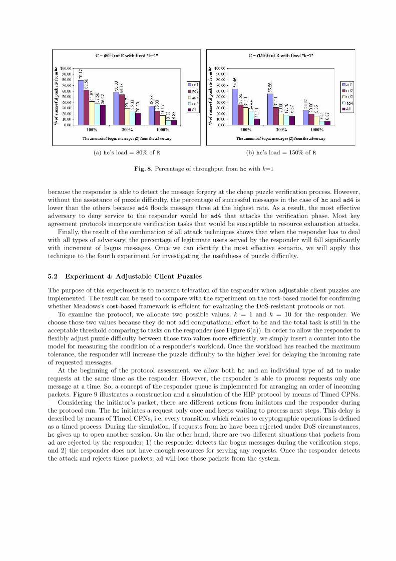
(a) hc’s load = 80% of R (b) hc’s load = 150% of R

Fig. 8. Percentage of throughput from hc with k=1

because the responder is able to detect the message forgery at the cheap puzzle verification process. However,without the assistance of puzzle difficulty, the percentage of successful messages in the case of hc and ad4 islower than the others because ad4 floods message three at the highest rate. As a result, the most effectiveadversary to deny service to the responder would be ad4 that attacks the verification phase. Most keyagreement protocols incorporate verification tasks that would be susceptible to resource exhaustion attacks.

Finally, the result of the combination of all attack techniques shows that when the responder has to dealwith all types of adversary, the percentage of legitimate users served by the responder will fall significantlywith increment of bogus messages. Once we can identify the most effective scenario, we will apply thistechnique to the fourth experiment for investigating the usefulness of puzzle difficulty.

5.2 Experiment 4: Adjustable Client Puzzles

The purpose of this experiment is to measure toleration of the responder when adjustable client puzzles areimplemented. The result can be used to compare with the experiment on the cost-based model for confirmingwhether Meadows’s cost-based framework is efficient for evaluating the DoS-resistant protocols or not.

To examine the protocol, we allocate two possible values, k = 1 and k = 10 for the responder. Wechoose those two values because they do not add computational effort to hc and the total task is still in theacceptable threshold comparing to tasks on the responder (see Figure 6(a)). In order to allow the responder toflexibly adjust puzzle difficulty between those two values more efficiently, we simply insert a counter into themodel for measuring the condition of a responder’s workload. Once the workload has reached the maximumtolerance, the responder will increase the puzzle difficulty to the higher level for delaying the incoming rateof requested messages.

At the beginning of the protocol assessment, we allow both hc and an individual type of ad to makerequests at the same time as the responder. However, the responder is able to process requests only onemessage at a time. So, a concept of the responder queue is implemented for arranging an order of incomingpackets. Figure 9 illustrates a construction and a simulation of the HIP protocol by means of Timed CPNs.

Considering the initiator’s packet, there are different actions from initiators and the responder duringthe protocol run. The hc initiates a request only once and keeps waiting to process next steps. This delay isdescribed by means of Timed CPNs, i.e. every transition which relates to cryptographic operations is definedas a timed process. During the simulation, if requests from hc have been rejected under DoS circumstances,hc gives up to open another session. On the other hand, there are two different situations that packets fromad are rejected by the responder; 1) the responder detects the bogus messages during the verification steps,and 2) the responder does not have enough resources for serving any requests. Once the responder detectsthe attack and rejects those packets, ad will lose those packets from the system.

Fig. 9. Protocol Steps of HIP Timed CPNs Model

The Experimental Results: To adjust the puzzle difficulty, we allocate two possible values for the respon-der to determine. Under normal circumstances, the responder selects k=1, which means the easiest puzzlesolution is required from the initiator. Once the responder receives more requested packets than its maximumcapacity to handle, the responder raises the puzzle difficulty. In the experiments described here, we choosek=10. Because this puzzle technique is a hash-based puzzle, this value will help the responder to slow downthe incoming rate by requiring the work of the initiator to solve puzzles at the factor of 210.

Similar to the representation of Figure 8, Figure 10 illustrates that the number of attacking machinesthat the responder can tolerate is increased to a higher proportion compared to the result of experiment1. Another interesting result is that the successful rate of an honest client’s message in the case of ad4 ishigher than for the fixed value k=1. The reason is that ad4 does not compute the puzzle solution, so, nomatter what the puzzle difficulty is, ad4 can flood the bogus messages at the similar speed as experiment 1.However, at that amount of bogus messages, there are only messages from ad4 (no legitimate traffic becausehc has to spend some amount of time to solve the puzzle solution), or just a few messages from hc thatarrive to the connection queue before the responder increases puzzle difficulty. As a result, the respondercan validate the puzzle solution before the next group of messages has arrived. Undoubtedly, these bogusmessages from ad4 will be rejected at the first step of verification which requires only a short period and

(a) hc’s load = 80% of R (b) hc’s load = 150% of R

Fig. 10. Percentage of throughput from hc with k is chosen between 1 and 10

removes such attacks from the connection queue. However, this situation does not occur in the case of ad3because they have to spend some amount of time to solve the puzzle as well as hc.

6 Conclusion and Future Work

This work has achieved the aims of extending the Meadows’s cost-based framework to provide more accuraterepresentation of computational cost and shown the potential of automated analysis. Moreover, we haveexplored unbalanced computational vulnerabilities on HIP which cause the responder to deplete resourcesand then terminate all processes by developing formal analysis based on Meadows’s cost-based frameworkand Time CPNs simulation-based analysis. By comparing experimental results from both techniques, wehave found a limitation of Meadows’ framework to define the ability of advanced adversaries and addressDoS vulnerabilities in DoS-resistant protocols.

In future work, we plan to extend this research by using the model checking capabilities of CPN tools toautomatically verify the system by traversing the model and checking whether the cost tolerance betweeninitiator and responder exceeds some reasonable threshold. Moreover, the power of adversaries can be ex-tended in different ways in order to model more powerful attacks. For example, the advanced adversary, whoattempts to attack the protocol at the third message, can be extended to flood reused packets from pre-vious connections, eavesdrop messages from a valid communication, or craft bogus messages using existingmessages including valid or invalid puzzle solutions as well as digital signatures. By inserting such advancedabilities to the model, we also require a technique to measure and identify cost of those operations in orderto achieve a formal analysis.

In addition there are a number of other promising directions for this research.

– Our model can be used to analyse a variety of protocols to provide a comparison of the effectiveness ofdifferent protocols in DoS prevention.

– Our model can be integrated into a model for security analysis of authentication and key establishmentproperties to create a unified protocol analysis tool covering resistance to DoS attacks as well as moretraditional security goals.

References

1. W. Aiello, S. M. Bellovin, M. Blaze, J. Ioannidis, O. Reingold, R. Canetti, and A. D. Keromytis. Efficient, DoS-resistant, secure key exchange for internet protocols. In the 9th ACM conference on Computer and communicationssecurity, pages 48–58, Washington, DC, USA, 2002. ACM Press.

2. I. Al-azzoni. The Verification of Cryptographic Protocols using Coloured Petri Nets. Master of Applied SciencesThesis, Department of Software Engineering, McMaster University, Ontario, Canada, 2004.

3. T. Aura, A. Nagarajan, and A. Gurtov. Analysis of the HIP Base Exchange Protocol. In Proceedings of 10thAustralasian Conference on Information Security and Privacy (ACISP 2005), volume 3574 of Lecture Notes inComputer Science, pages 481 – 493, Brisbane, Australia, Jun 2005. Springer-Verlag.

4. T. Aura and P. Nikander. Stateless Connections. In International Conference on Information and Communica-tions Security, pages 87–97, Beijing, China, Nov 1997. Springer-Verlag.

5. T. Aura, P. Nikander, and J. Leiwo. DoS-resistant authentication with client puzzles. In Security ProtocolsWorkshop 2000, pages 170–181. Cambridge, Apr 2000.

6. J. Beal and T. Shepard. Deamplification of DoS Attacks via Puzzles. Available: http://web.mit.edu/jakebeal/www/Unpublished/puzzle.pdf, 2004.

7. Computer Emergency Response Team (CERT). Denial-of-Service Attack via ping. [Online]. Available: http://www.cert.org/advisories/CA-1996-26.html [Accessed: August 2004], 1996.

8. Computer Emergency Response Team (CERT). TCP SYN Flooding and IP Spoofing Attacks. [Online]. Available:http://www.cert.org/advisories/CA-1996-21.html, 1996.

9. S. Christensen and K. H. Mortensen. Teaching Coloured Petri Nets- A Gentle Introduction to Formal Methodsin a Distributed Systems Course. In ICATPN, pages 290–309, 1997.

10. Wei Dai. Crypto++ 5.2.1 Benchmarks. [Online]. Available: http://www.eskimo.com/∼weidai/benchmarks.html[Accessed: Nov 2005], 2004.

11. E. M. Doyle. Automated Security Analysis of Cryptographic Protocols using Coloured Petri Net Specification.Master of Science Thesis, Department of Electrical and Computer Engineering, Queen’s University, Ontario,Canada, 1996.

12. A. O. Freier, P. Karlton, and P. C. Kocher. The SSL Protocol Version 3.0. Internet Draft, Internet EngineeringTask Force, November 1996. http://wp.netscape.com/eng/ssl3/draft302.txt.

13. V. Gupta, S. Gupta, S. Chang, and D. Stebila. Performance Analysis of Elliptic Curve Cryptography for SSL.In WISE’02: Proceedings of the 3rd ACM Workshop on Wireless Security, pages 87–94, Atlanta, GA, USA, 2002.ACM Press.

14. Y. Han. Automated Security Analysis of Internet Protocols using Coloured Petri Net Specification. Master ofScience Thesis, Department of Electrical and Computer Engineering, Queen’s University, Ontario, Canada, 1996.

15. M. Jakobsson and A. Juels. Proofs of work and bread pudding protocols. In the IFIP TC6 and TC11 JointWorking Conference on Communications and Multimedia Security (CMS 99), Sep 1999. Also available ashttp://citeseer.nj.nec.com/238810.html.

16. K. Jensen. Coloured Petri Nets: Basic Concepts, Analysis Methods and Practical Use. Springer-Verlag, 2ndedition, Vol. 1-3, April, 1997.

17. A. Juels and J. Brainard. Client Puzzles: A Cryptographic Defense Against Connection Depletion Attacks. In the1999 Network and Distributed System Security Symposium (NDSS ’99), pages 151–165, San Diego, California,USA, Feb 1999. Internet Society Press, Reston.

18. P. Karn and W. A. Simpson. Photuris: Session-Key Management Protocol. Experimental RFC 2522, IETF, Mar1999. http://www.ietf.org/rfc/rfc2522.txt.

19. C. Meadows. A Cost-Based Framework for Analysis of DoS in Networks. Journal of Computer Security,9(1/2):143–164, Jan 2001.

20. H. C. Moon. A study on formal specification and analysis of cryptographic protocols using Colored Petri Nets.Master of Science Thesis, Institute of Science and Technology, Kwangju University, Korea, 1998.

21. R. Moskowitz. The Host Identity Protocol (HIP). Internet Draft, Internet Engineering Task Force, Jun 2006.http://www.ietf.org/internet-drafts/draft-ietf-hip-base-06.txt.

22. B. B. Neih and S. E. Tavares. Modelling and Analysis of Cryptographic Protocols using Petri Nets. In Advancesin Cryptology, pages 275–295, Berlin, German, 1993.

23. C. A. Petri. Kommunikation mit Automaten. PhD Thesis, Institut fur Instumentelle Mathematik, Schriffen desIIM, 1962.

24. J. Smith, J. M. Gonzalez Nieto, and C. Boyd. Modelling Denial of Service Attacks on JFK with Meadows’s Cost-Based Framework. In Fourth Australasian Information Security Workshop (AISW-NetSec 2006), volume 54,pages 125–134. CRPIT series, 2006.

25. J. Smith, S. Tritilanunt, C. Boyd, J. M. Gonzalez Nieto, and E. Foo. DoS-Resistance in Key Exchange. Interna-tional Journal of Wireless and Mobile Computing (IJWMC), 1(1), Jan 2006.

26. Z. Tan, C. Lin, H. Lin, and B. Li. Optimization and Benchmark of Cryptographic Algorithms on NetworkProcessors. IEEE Micro, 24(5):55–69, Sept/Oct 2004.

27. The Department of Computer Science, University of Aarhus, Denmark. CPN Tools: Computer Tool for ColouredPetri Nets. [Online]. Available: http://wiki.daimi.au.dk/cpntools/cpntools.wiki, 2004.

Game Coloured Petri Nets

M. Westergaard

Department of Computer Science, University of Aarhus,IT-parken, Aabogade 34, DK-8200 Aarhus N, Denmark,

Email: [email protected]

Abstract. This paper introduces the notion of game coloured Petri nets.This allows the modeler to explicitly model what parts of the modelcomprise the modeled system and what parts are the environment of themodeled system. We give the formal definition of game coloured Petrinets, a means of reachability analysis of this net class, and an applicationof game coloured Petri nets to automatically generate easy-to-understandvisualizations of the model by exploiting the knowledge that some partsof the model are not interesting from a visualization perspective (i.e. theyare part of the environment, and not controllable by the system itself, orthey are part of the system itself and therefore we need not worry aboutthem).

1 Introduction

The coloured Petri nets (CPNs or CP-nets) [14] formalism has proven itself usefulfor modeling concurrent systems such as network protocols [11,12,17,18,21] andworkflows [4, 15]. One problem that is often encountered is how to distinguishbetween the system itself and its environment [30], as we would often like tomake the assumptions about the environment explicit even though they are notdirectly part of the system we want to model. Normally we would model theenvironment simply as a part of the model and at best accompany the modelby an informal textual description of what parts of the model comprise theenvironment or, at worst, let this information be implicit. If the modeler is a bitmore thorough, he will split the model up into separate modules and put theenvironment in certain modules and the modeled system in other modules. Theproblem with the first of approach is that the information about which partsof the model are the actual system is not part of the modeled system, therebymaking it impossible to use this information during analysis or other treatmentsof the model. If, on the other hand, we put the model of the environment inseparate modules, we may obtain an unnatural model in which the natural flowof the system is not readily visible if the flow consists of frequent interleavingsof actions between the modeled system and the environment.

In this paper we will study another way to model the environment forcoloured Petri nets. The idea is to separate the actions of the system into twoparts, the controllable and the uncontrollable actions. The controllable actionsare, as the name suggests, controllable by the system we model. The system can

choose which and when to execute controllable actions, e.g. transmit a packetonto the network. The uncontrollable actions are not controllable by the system,but can occur whenever they are enabled. The inspiration of this is classicalgames such as tic-tac-toe, in which two players, cross and naught, play againsteach other. Say we model the game from the point of view of the player drawingcrosses. The action of adding a new cross to the board is controllable, whereasthe action of adding a naught is uncontrollable.

While it is interesting in itself to be able to study small toy-games such astic-tac-toe using coloured Petri nets, the real power of separating the actionsinto uncontrollable and uncontrollable ones comes when regarding more realisticexamples, e.g. a model of a network protocol. The network protocol contendsagainst the network, which may lose packets, duplicate packets, or even alterpackets. In this case all actions of the protocol (such as retransmitting a packet)are controllable, whereas the actions of the environment (such as transmittingor dropping the packet) are uncontrollable. This illustrates how separating theactions into controllable and uncontrollable actions allow us to explicitly spec-ify what parts of the model comprise the system and what parts comprise theenvironment. Actions of the system are modeled as controllable transitions (byconvention drawn as a rectangle) and actions of the environment are modeled asuncontrollable transitions (drawn as a dashed rectangle). Allowing this distinc-tion directly in the model has several uses. Firstly, it alleviates the need for aninformal textual description of which parts of the model are the modeled, inter-esting system, and which parts just make the assumptions of the environmentexplicit. Secondly, we can use the distinction to do better analysis of the prop-erties of the system, and to automatically generate strategies (corresponding toprograms) making sure, e.g. that the system always reaches a state where allpackets have been successfully transmitted. Thirdly, we can use the extra infor-mation to generate visualizations of the system allowing users to interact withthe model without looking at the model. We could have chosen to distinguishcontrollable actions from uncontrollable actions on the level of tokens or transi-tion modes, but have chosen to make the distinction on the level of transitionsfor simplicity. Refer to the conclusion (Sect. 6) for a brief discussion of anotherway to do the distinction.

The contribution of this paper is three-fold: The introduction of game colouredPetri nets, the adaptation of an algorithm for reachability analysis of finitegames [2] to game coloured Petri nets, and, thirdly, an application of gamecoloured Petri nets to automatically tie CPN models to visualizations.

The rest of this paper is structured as follows: Firstly, in Sect. 2, we willgive an informal introduction to game CP-nets and introduce a simple example,which will be used in the rest of the paper. Secondly, in Sect. 3, we will formalizethe notion of game coloured Petri nets (game CPNs or game CP-nets). In Sect. 4,we outline how to do reachability analysis of game CP-nets. After that we willturn to a simple yet powerful application of games to automatically generatevisualizations of CPN models. Finally, we will give our conclusions and providedirections for future research in Sect. 6.

2 Example

In this section, we will introduce a simple example game CP-net, which we willuse in the following sections. The example is a slight modification of one of thesample nets supplied with CPN Tools, namely a simple stop-and-wait protocol.

The modified example can be seen in Fig. 1. In the example, a sender, on theleft, wants to transmit some packets lying on the place Send. The sender has acounter telling which packet to send next, NextSend. When the transition Send

Packet occurs, it puts the packet onto the network (place A). Now the network,in the middle of the model, can either choose to Transmit Packet or Drop Packet.These two actions are uncontrollable, modeling that the protocol has no controlover what happens on the network. If the packet is dropped, it is simply removedfrom place A, otherwise it is moved onto place B, where the receiver, on theright of the model, can Receive Packet. When this happens, either the packetis received for the first time or it is a retransmission. The receiver keeps trackof which packet it expects by a counter on the place NextRec. If the sequencenumber of the incoming packet is not equal to the expected sequence number, thepacket is discarded. Otherwise, the new packet is stored on the place Received.In either case, an acknowledgment is sent back to the network by putting atoken on place C, containing the sequence number of the next expected packet.The acknowledgment can be either transmitted or dropped by the network. If itarrives safely on place D the sender can Receive Ack, and update the number ofthe next packet to send, and start a new cycle sending the next packet.

nn

n k

n n

if n=kthen k+1else k

k

n

if n=kthen 1`pelse empty

(n,p)

(n,p)

(n, p)(n,p)(n,p)

TransmitAck

ReceiveAck

ReceivePacket

TransmitPacket

SendPacket

C

INT

B

INTxDATA

1

DATA

A

INTxDATA

D

INT

NextSend

1

INT

Send


Received

INTxDATA

INT

1`(1,"Bored? P")++1`(2,"lay game")++1`(3,"CP-nets!")

NextRec

n

DropAck

(n,p) DropPacket

Fig. 1. A simple stop-and-wait protocol modeled using game CP-nets.

In this example we have modeled all actions of both sender and receiver ascontrollable and all actions of the network as uncontrollable. That is, we regardthe network protocol as the modeled system and the network as the environment.We could have modeled the actions of e.g. the receiver as uncontrollable as well,thereby only regarding the sender as the modeled system.

3 Formal Definition

In this section we will give a formal definition of game coloured Petri nets (gameCPNs or game CP-nets). The intuition of the definition is that we partition theset of transitions into controllable and uncontrollable transitions. We will do thisby first recalling the definition of standard coloured Petri nets.

We will assume that the relations <, =, ≤, >, and ≥, and operations +and −, on multi-sets are defined as usual. We use N

S to denote the set of allmulti-sets over S.

Definition 1 (Coloured Petri net (Def. 5.1 and 5.2 in [13]1)). A colouredPetri net is a tuple, CPN = (P, T, D, Type, Pre, Post, M0), where

– P is a finite set of places,– T is a finite set of transitions such that P ∩ T = ∅,– D 6= ∅ is a finite set of non-empty types,– Type : P ∪ T → D is a type function assigning a type to each place and

transition,

– TRANS = {(t, m) | t ∈ T, m ∈ Type(t)} is the set of all transition modes,– N

PLACE = N{(p,g) | p∈P,g∈Type(p)} is the set of all markings,

– Pre, Post : TRANS → NPLACE are the backward and forward incidence

functions, assigning to each arc an annotation, and

– M0 ∈ NPLACE is the initial marking.

The state of a CP-net is given by a marking of the places, which is a multi-set,M ∈ N

PLACE .

Definition 2 (Enabling and occurence of transitions (Def. 5.3.1 and

5.4 in [13])). A transition mode, (t, m) ∈ TRANS, is enabled in marking

M ∈ NPLACE if Pre(t, m) ≤ M . A transition t ∈ T is enabled if there exists

m ∈ Type(t) such that (t, m) is enabled. If (t, m) is enabled in M , it may occur

and lead to a marking M ′. This is written M(t,m)→ M ′, where M ′ is defined by

M ′ = M − Pre(t, m) + Post(t, m).

Definition 3 (Game coloured Petri net). A game coloured Petri net (game

CP-net or GCPN) is a tuple, GCPN = (P, Tc, Tu, D, T ype, Pre, Post, M0, W ),where

– Tc is a finite set of controllable transitions,– Tu is a finite set of uncontrollable transitions such that Tc ∩ Tu = ∅,– CPN = (P, Tc ∪ Tu, D, T ype, Pre, Post, M0), the underlying coloured Petri

net, is a coloured Petri net, and

– W : NPLACE → {tt, ff} is a predicate identifying winning markings.

1 In this paper we will use the term coloured Petri net rather than high-level Petri netas used in [13].

The notions of markings, transition modes, enabling, and occurrence for gameCP-nets are the same as for coloured Petri nets. Furthermore, we shall allowthe notation TRANSc = {(t, m) | t ∈ Tc, m ∈ C(t)} for the controllable transi-

tion modes and TRANSu = {(t, m) | t ∈ Tu, m ∈ C(t)} for the uncontrollable

transition modes

One thing to note is that we do not impose any ordering on controllable oruncontrollable actions. We could have required that a controllable action mustalways be followed by an uncontrollable action and vice versa, but we will notdo this, as enabling suddenly becomes dependent on the level of detail used tomodel the system. If such behavior is required (e.g. in the case of the tic-tac-toegame), it must be modeled explicitly. We will discuss this further in Sect. 5.4,where we talk about fairness when using game CP-nets to automatically generatevisualizations of models.

4 Analysis

For finite games, i.e. games constructed by separating the actions of finite au-tomata into controllable and uncontrollable actions, we can do several kinds ofanalysis. One of the simplest properties we can check is a reachability prob-lem, namely whether it is possible to find a strategy ensuring we will end up inone of the winning states. A strategy is a mapping from states to controllabletransitions. A strategy is a winning strategy iff we are ensured, no matter whatuncontrollable transitions are executed, to end up in one of the winning statesif we in every state pick the transition specified by the strategy. The reacha-bility property is interesting when the set of the winning states, W , representdesirable final markings, e.g. that all packages have been received successfully.A winning strategy corresponds to a recipe for what the modeled system shoulddo in order to ensure it will end up in a desirable state. Using a solution for thesimple reachability problem, we can also solve the dual safety problem, whetherwe can ensure that no matter which uncontrollable transitions are executed,we will never reach a state which is not winning. This property is interestingfor reactive systems, where the set W corresponds to states where nothing badhas happened, e.g. that the system has not dead-locked or received a damagedpacket.

Rather than going through the definitions required to solve the reachabilityproblem directly for game CP-nets, we will go through how to translate thereachability problem for game CP-nets into a reachability problem for finitestate systems. This, of course, cannot be done in general (as the reachabilitygraph of the underlying CP-net can be infinite), but we do it in a way thatensures that if the reachability graph of the underlying CP-net is finite, thealgorithm will terminate with the correct answer.

In [5], Cassez, David, Fleury, and Larsen instantiate an algorithm by Liuand Smolka from [19] to obtain an efficient (and optimal) algorithm to decidewhether a given finite reachability game has a winning strategy and to extractthat strategy. The intuition of the algorithm is to calculate a minimal fix-point of

all good states, Win, where all states in W are good and all states where we cantake a controllable step to a good state and all uncontrollable steps lead to a goodstate are good. This corresponds to the intuition that in any given state, we havea winning strategy if we can execute a controllable transition and end in a newstate where we have a winning strategy, and that no matter what the opponentdoes, we end up in a state where we have a winning strategy. The algorithmassumes a finite game as a tuple (Q, q0, Actc, Actu, δ, Goal) (all states, the initialstate, the controllable and uncontrollable actions, the transition relation, andthe winning states). The adaptation of the algorithm to game CP-nets is easy.Given a game CP-net, GCPN = (P, Tc, Tu, D, T ype, Pre, Post, M0, W ), we willassume that all types in D are finite and that the number of tokens on allplaces are bounded. Then we can take Q = N

PLACE , Actc = TRANSc, andActu = TRANSu, all of which are finite. We set Goal = W , q0 = M0, and let

δ = {(M, (t, m), M ′) |M(t,m)M ′

→ }. We then obtain Algorithm 1. The algorithmworks by forward traversal of the reachability graph. Whenever a state is foundto be winning, it is added to Win (ll. 3, 10, and 19). Whenever we find a newstate, we mark it as dependent on the winning status of its successors (ll. 9 and22). When a state is marked as winning, we schedule all states dependent on itswinning status for re-evaluation (ll. 13 and 18). With a little cleverness in theimplementation of line 162, the algorithm is shown to find a winning strategy intime linear in the number of nodes and edges in the reachability graph. We usethe standard notation that the empty conjunction is tt and the empty disjunctionis ff.

A nice property of this algorithm is that the while loop (ll. 5–25) has the in-variant that if Win[M ] = tt then there exist a winning strategy for GCPN wherewe use M as the initial marking (rather than M0). Furthermore this invariantholds irregardless of which element the operation pop picks in line 6. The firstproperty allows us to implement early termination by adding the additional con-straint Win[M0] 6= tt to the while loop in line 5, and the second property allowsus to do more intelligent search for winning strategies. The algorithm has beenimplemented in the model checker included in the BRITNeY Suite [28,29]. Thecurrent implementation uses either a simple depth-first search or a breath-firstsearch. The depth-first search has a tendency to find winning strategies fasterthan the breath-first search, as it favors making controllable moves rather thanwaiting for the opponent to make “good” uncontrollable moves. More intelligentsearch can be made by making e.g. an α − β search [25] as known from the AIworld to allow computers to play difficult games, such as chess.

2 Rather than re-evaluating both the conjunction and the disjunction each time wereach this line, we notice that the entire expression is true iff just one state reachableby a controllable action is winning and if all states reachable by uncontrollableactions are winning. Using an integer to keep track of how many states reachableby an uncontrollable action are currently not marked as winning and a boolean tokeep track of whether a state reachable by a controllable action has been marked aswinning, we only do a constant amount of work each time we need to re-calculationthe expression.

Algorithm 1 SolveGCPN

Require: GCPN = (P, Tc, Tu, D, Type,Pre,Post, M0, W ), a game CP-net1: Storage← {M0}

2: Waiting← {(M0, (t, m), M ′) |M0(t,m)→ M ′}

3: Win[M0]←W (M0)4: Depend[M0]← ∅5: while Waiting 6= ∅ do

6: (M, (t, m), M ′)← pop(Waiting)7: if M ′ /∈ Storage then

8: Storage← Storage ∪ {M ′}9: Depend[M ′]← {(M, (t, m), M ′)}

10: Win[M ′]← W (M ′)

11: Waiting← Waiting ∪ {(M ′, (t′, m′), M ′′) |M ′(t′,m′)→ M ′′}

12: if Win[M ′] then

13: Waiting←Waiting ∪ {(M, (t, m),M ′)}14: end if

15: else {reevaluate}16: Win∗ ←

V

(tu,mu)∈TRANSu, M

(tu,mu)→ M

′

Win[M ′] ∧W

(tc,mc)∈TRANSc, M

(tc,mc)→ M

′′

Win[M ′′]

17: if Win∗then

18: Waiting←Waiting ∪ Depend[M ]19: Win[M ]← tt

20: end if

21: if Win[M ′] then

22: Depend[M ′]← Depend[M ′] ∪ {(M, (t,m), M ′)}23: end if

24: end if

25: end while

Due to the general result of [19], we can replace the calculation in line 16 ofthe algorithm with any monotone property (any propositional formula not usingnegation or implication). For example, we may find that it is more intuitive thata state is winning if we have a controllable move leading to a winning state or

all uncontrollable moves lead to winning states.We also notice that we never use that N

PLACE (the syntactically possiblestates of GCPN ) is finite, but only that the reachable states of GCPN are, so wecan in fact remove the requirement that all types in D are finite as long as weonly use a finite subset of the values. This allows us to analyze arbitrary gameCPN models using the algorithm. If the algorithm terminates, we will know thatthe result is correct (due to the loop invariant, which is proven correct in [5]).

4.1 Experimental Results

We cannot directly analyze the network protocol from the previous example,as the place A is unbounded (and the algorithm will keep executing the Send

Packet transition, which remains enabled). However, if we put a bound on thenumber of tokens on the places A, B, C, and D, we can analyze the model. Wewill then discover that there is no winning strategy (the network can just keepon throwing away packets). If we furthermore limit the number of times thenetwork can drop packets, we will find that we have a winning strategy. Whenwe add a limit on the number of packets on the network and limit the numberof times a packet can be lost, we obtain the model in Fig. 2. The only changesfrom the original net in Fig. 1 is that we have added two new places Capacity

(bounding the number of tokens on A, B, C, and D) and May lose (bounding thenumber of times Drop Packet and Drop Ack can fire). Also the place NextRec hasbeen moved to improve the layout.

()()

()

()

()

(n,p)

n

nn

n k

n n

k

n


if n=kthen 1`pelse empty(n,p)

(n,p)

(n, p)(n,p)(n,p)

DropPacket

DropAck

TransmitAck

ReceiveAck

ReceivePacket

TransmitPacket

SendPacket

Capacity

UNIT

Maylose

UNIT

C

INT

B

INTxDATA

NextRec

1

INT

Received

DATA

A

INTxDATA

D

INT

NextSend

1

INT

Send1`(1,"Bored? P")++1`(2,"lay game")++1`(3,"CP-nets!")INTxDATA

() ()()


Fig. 2. The stop-and-wait protocol modified for analysis.

We have conducted four series of experiments: two for the model in Fig. 2and two for the same model but with the May lose place and all connected arcsremoved (i.e. removing the limit on the number of packet losses). For each ofthe two models, we have conducted two series of experiments, one without earlytermination and one with early termination, where we allow the algorithm toterminate as soon as we have a proof either for or against the existence of awinning strategy. Each series consists of a number of experiments with varyingcapacity and bound of the number of packets we may lose. We regard as winningstates the states where all packets has been received successfully. All series areconducted using a recursive depth-first traversal and using double hashing [8]with 15 combinations and 108 buckets for the Win and Storage data-structures(resulting in a total memory use of about 25 MiB). Depend is represented implic-itly on the recursion stack. The experiments are not meant to show the generalperformance of the algorithm, as this has already been done in [5], but they aremeant to give an impression of the performance of the algorithm when adaptedto game CP-nets. All experiments are conducted on an Apple MacBook Pro with

a 2.16 GHz Intel Core Duo processor3 and 2 GiB RAM, using BRITNeY Suiteversion 0.9.75.101.

In Table 1, we see the results from analysis of the model with no limit on thenumber of losses of packets. The table has 6 columns. The first column, Early

termination allowed, indicates whether early termination is allowed or not. Thesecond column, Tokens on Capacity place, indicates how many tokens the placeCapacity contains initially. The columns Storage and Win indicates how manystates are stored in the corresponding data-structures. Note that we do not storestates with no successors in Storage (as they are winning iff they are contained inWin), which is why the number of winning states may be larger than the numberof stored states. The next column, Winning strategy exists indicates whether thealgorithm concludes that a winning strategy exists. The final column, Execution

time, indicates how long time (in seconds) the algorithm used to reach thatconclusion.

The first thing we notice is that early termination really speeds the cal-culation up. It seems that the time spent increases exponentially without andquadratically with early termination. This is a lucky coincidence in this model,as the algorithm can easily see that no matter how many packets we pump ontothe network, the network can just drop them and leave us at the initial state,thereby preventing us from even getting started with the protocol. We also notethat it seems like the algorithm has a start-up cost of about 0.1 second, whichis probably used for allocating the bit-arrays used for storing states.

In Table 2 we see the results for the analysis with a limit on the number ofpackets the network is allowed to lose. The columns have the same meaning asin Table 1, except we have added a column, Tokens on May lose place, whichcontains the number of tokens initially on the May lose place.

We notice that the algorithm now states that we do indeed have a winningstrategy (and gives us a function which returns for each reachable state whichevent we should execute in order to win). Furthermore, we notice that when we donot allow early termination, the number of states and the execution time growsapproximately linearly in the number of allowed losses (which makes sense, as webasically have a copy of the entire reachability graph for each possible markingof May lose). We also note that the number of states and the execution timewhen no packets can be lost correspond approximately to the number of stateswhen we allow an arbitrary number of packet losses (this also makes sense, as apacket loss basically goes back an event).

When we allow packet loss, we see, again, that the number of states andthe execution time grows linearly with the number of packets the network canlose, and they seem to grow quadratically in the capacity of the network. Thecalculation is significantly more difficult than before, when there was no limiton the number of packets we can lose, as we will have to search deeper for awinning strategy than we did to find a counterexample previously. We also notea significant speedup compared to not allowing early termination.

3 The processor contains two cores, but the analysis is currently only able to use oneof them.

Table 1. Data from analysis of the network model in Fig. 2 without limit on numberof losses (i.e. the May lose place and its surrounding arcs have been removed).

Early Tokens on Winning Executiontermination Capacity Storage Win strategy time

allowed place exists (seconds)

No

1 20 2 ff 0.1532 115 32 ff 0.1714 1807 1032 ff 0.5886 14917 11508 ff 3.2088 83173 76208 ff 22.046

10 355842 365770 ff 115.459

Yes

1 3 0 ff 0.1112 4 0 ff 0.116

10 12 0 ff 0.145100 102 0 ff 0.282500 502 0 ff 3.392

1000 1002 0 ff 12.3382000 2002 0 ff 55.8092800 2802 0 ff 123.180

When we have found a winning strategy (or concluded that no winning strat-egy exists), we would like to show this strategy to the user. Ways to do thisinclude printing all reachable markings and the winning move or to annotate agraphical representation of the reachability graph with the suggested move. Thisis very easy to implement, but not very good to convince users. A better way topresent a winning strategy to a user is presented in the next section.

5 Automatically Generated Visualizations

While CP-nets are graphical and can be communicated to computer scientists,they contain a lot of details that are not needed to grasp the essentials of amodel. Often we also need to communicate the ideas of the model to domainexperts in order to validate that the constructed model actually represents theproblem domain. In order to facilitate easy communication of (CPN) models, alot of tools [10, 16, 24, 29] have been conceived with the purpose of constructingdomain specific visualizations. These tools either mainly allows simple inspectionof the state of the model during execution, or requires that the modeler spendsa lot of time constructing an visualization and tying it to the model.

Using the concept of games, we can do better. Firstly, we notice that visual-izations often allow the user to experiment with the modeled system and observehow the system reacts to different stimuli, thereby playing the role of the envi-ronment. Another kind of visualization allows the user to play the role of themodeled system, contending against the environment. Both of these correspondnicely to how we play a game. We make a move and observe how the opponent

Table 2. Data from analysis of the network model in Fig. 2.

Early Tokens on Tokens on Winning Executiontermination Capacity May lose Storage Win Winning Time

allowed place place exists (seconds)

No

4 0 1732 2248 tt 0.3404 1 3538 4570 tt 0.6024 5 10762 13858 tt 1.6794 50 92032 118348 tt 18.7524 200 362930 466638 tt 140.8918 0 82768 120871 tt 16.5618 1 165939 242146 tt 39.6758 5 498612 727198 tt 131.478

Yes

4 200 10903 11688 tt 1.8478 5 290 297 tt 0.147

10 0 50 51 tt 0.14410 1 185 192 tt 0.14710 10 737 757 tt 0.23210 100 12134 13043 tt 1.59410 1000 126699 136647 tt 71.22810 2000 253778 273733 tt 260.406

100 0 410 411 tt 0.335100 1 825 827 tt 0.561100 10 4608 4625 tt 1.638100 100 43630 43946 tt 14.112100 500 438319 467416 tt 247.340500 73 149511 149636 tt 246.562

1000 17 72265 72283 tt 247.0271500 3 24055 24059 tt 294.097

reacts. So, basically, what we want to is to allow an external visualization com-ponent to control one side of the game and let the tool control the other side. Inour example, we can let the user control the controllable actions, thereby takingthe role of the protocol, or let the user play the role of the environment, therebyletting the user try to make the protocol fail. As the distinction between themodeled system and the environment is part of the model in game CP-nets, itis possible to automatically execute transitions from the environment when theuser plays the role of the modeled system (and vice versa).

The rest of this section starts by introducing two simple kinds of automati-cally generated visualization, then goes on to discuss fairness during the visual-ization, and finally extends the scope to more general visualizations. All of thevisualizations presented in this section have been implemented in the BRITNeYSuite [28, 29].

5.1 Binding Index Inspired Visualization

CPN Tools allows users to select specific modes for each transition by usingbinding indexes (in CPN Tools the notion of a high-level Petri net Graph [13,Sects. 7–9] is used, where binding elements, a transition and an assignment ofvalues to variables on the surrounding arcs, correspond to transition modes). InFig. 3 we see an example of a binding index in CPN Tools. Here the transitionTransmit Packet is enabled, and the variable n can be assigned either the value 1

or 2, and the variable p can be assigned either ”Bored? P” or ”lay game”. Bindingindexes make it possible to exercise very detailed control of the model, but alsorequires the user to browse through the entire model to find enabled transitionsand to select the desired mode.

Fig. 3. A binding index from CPN Tools.

One way to automatically generate a “visualization” is to simply show theuser a list of all enabled binding elements (i.e. hide any binding elements cor-responding to uncontrollable transitions and execute them automatically). Anexample of this can be seen in Fig. 4. Here we see that the transitions Receive

Packet and Send Packet are enabled. We also see that Receive Ack is disabled(normally the list of disabled transitions are hidden, but they can be made vis-ible by the user by clicking on the double arrow). We have currently selectedthe Receive Packet transition, and we see that we can select one of two bindingelements. We note that we do not see any of the transitions for transmitting anddropping packets, as they are part of the environment and cannot be controlledby the user. At the top, we can see that the last move of the tool was to executethe transition Drop Packet and the values assigned to its surrounding variables.This visualization is very straightforward to implement and use, but requiresthat the user has a very detailed knowledge of the model (or that the model isvery simple).

A better way to automatically generate visualizations is to take the idea ofthe binding index a bit further. We will show a dialog for each enabled tran-sition. The dialog can be placed by the user, allowing him to arrange the con-structed work space at will, but will be opened/closed by the system dependingon whether the transition is enabled. Instead of just listing the possible assign-ments, the dialog contains well-known widgets for displaying booleans, integers,

Fig. 4. A visualization generated by showing enabled binding elements.

and strings. More complex types can currently be selected by selecting the val-ues from a list. An example of this can be seen in Fig. 5. Here three transitionsare enabled, Send Packet, Receive Packet, and Receive Ack. We can see that weare currently executing Send Packet as it is grayed out and a rotating progressindicator indicates that the transition is being executed. In the Receive Packet

window we see that K is assigned the value 3, N to 2, and P to ”Rocks”. Thesmall triangle with an exclamation mark near the input field of P indicates thatthe value selected is indeed valid, but it is inconsistent with the other values(the packet containing ”Rocks” has a sequence number of 3). We cannot changethe value of K—it is shown for informational purposes only (this feature can beused to display a message to the user, e.g. by adding a variable message andassigning it one of the values ”Please enter your name” or ”The packet has beentransmitted”, depending on what action is required of the user and the model).In the window for Receive Ack we see that K is assigned to 2 and N to 0. Thecircle with a cross indicates that the value is not valid, and another value shouldbe chosen.

Apart from being a natural way to select between available tokens, this vi-sualization also allows the user to generate new tokens by adding a controllablesource transition, which has free variables. This is also how we would normallygenerate new tokens in CPN Tools, but CPN Tools only allows users to bindvariables freely from “small colour sets”, which basically means booleans andenumerations. BRITNeY Suite extends this to also include strings and integers,which e.g. makes it possible to ask a user for name and age and use that laterin the model.

This visualization can also be used without using the notions of games, as weonly use the separation of transitions to make some choices on behalf of the user.In the next section we shall see an example of a visualization which cruciallydepends on the separation in order to work by using controllable actions toprovide stimuli to the model and uncontrollable actions to provide feedback tothe user.

Fig. 5. Visualization generated from the net using common widgets.

5.2 Visualization using SceneBeans

BRITNeY Suite integrates the SceneBeans [26] library for use with visualiza-tions. The library uses an XML specification for describing visualizations andallows the model to interact with the specified visualization by invoking com-mands in the visualization and receiving events from the visualization.

Normally the programmer would use the interface from Listing 1 and call thefunctions from declarations or from code segments attached to the transitionsof the model. The first two functions in Listing 1 are used to setup or reset thevisualization, invokeCommand (l. 5) is used to invoke commands in the visual-ization, which basically means to show some animation or feedback to the user.The next four functions, in lines 7–10, makes it possible to listen for events fromthe visualization (e.g. the user has clicked a certain object, dragged a certainobject, or some other action). The last two function makes it possible to set cer-tain values in the visualization, such as the position or color of an element. Theuse of this interface has a tendency to clutter the model and special precautionsmust be taken in order to turn the visualization on or off, e.g. for analysis.

Rather than letting the user tie the model and the visualization togethermanually, we shall identify events of the SceneBeans visualization with control-lable actions and commands with uncontrollable actions. Thus, whenever anevent is dispatched, the system will try to execute the corresponding transitionas soon as possible. If an uncontrollable transition is fired, the correspondingcommand (if one exists) will be called. We shall identify events and commandswith transitions simply by name. A more complex mapping can be made (e.g.by introducing a “synchronize” predicate, which determines whether a transi-tion should be synchronized with a command or event), but we prefer this simpleapproach, as it is simpler to understand for the user, and eliminates the need tomanually specify such a predicate.

Listing 1 The interface to the SceneBeans library.1 signature SCENEBEANS = sig

2 val setAnimation: unit -> string

3 val reset: unit -> unit

4

5 val invokeCommand: string -> unit

6

7 val hasMoreEvents: unit -> bool

8 val getNextEvent: unit -> string

9 val peekNextEvent: unit -> string

10 val waitForEvent: string -> unit

11

12 val setValue: string * string * string -> unit

13 val getValue: string * string -> string

14 end

Suppose we have created an visualization showing two computers and a net-work. The visualization has commands for moving dots from one computer tothe other and vice versa as well as for dropping these dots from the cloud. Ifwe name these commands after the transitions, we can, without altering the netin Fig. 1 at all, generate a SceneBeans visualization like the one in Fig. 6. Herewe have a sender (on the left) and a receiver (on the right) and a network con-necting them. The dots represent data or acknowledgment packets sent over thenetwork. When a transition fires in the model, the visualization is automaticallyupdated. When we click on the sender, an event is generated, which causes thesender to send a packet, so initially the model does nothing (it waits for packetsto appear on the network). We can send as many packets as we want as fast aswe want. The model will transmit or drop the packets automatically. We couldalso have added a way to manually receive packets, but we have chosen that themodel can do this itself.

Fig. 6. SceneBeans visualization automatically synchronized with the model.

We note that we only have concepts corresponding to the command andevent parts of the SceneBeans interface. It would be very nice to extend theautomatic synchronization of SceneBeans visualizations and game CPN modelsto also include reading from and writing to properties of the visualization, forexample to show the NextSend and NextRec counters directly in the visualization,

or to attach package numbers to the dots. This could probably be done byassociating values in the visualization with tokens on global fusion places in thegame CPN model. How to do this is future work.

5.3 Intelligent Playing

Using the algorithm outlined in Sect. 4, we can allow the computer player toplay more intelligently by using the winning strategy (if one exists) as guidancerather than random selection.

In principle, this requires that we calculate the entire winning strategy be-forehand. As explained in Sect. 4, we know that we can use α − β heuristics tospeed up the search, and we can use early termination of the analysis algorithmto speed up the initial start up time. If a winning strategy is found during aprevious game, it can of course be reused during future visualizations.

Allowing the computer player to use a winning strategy is a nice way topresent a winning strategy to the user, as it may be difficult to grasp the winningstrategy as a mapping from states to transition modes. By allowing the userto play against the strategy, he can easily convince himself that the strategyproposed by the algorithm is indeed winning. All visualizations introduced inthis section can be used to demonstrate that a winning strategy is winning.

5.4 Fairness in Execution

When we make visualizations using games, we may need to impose some fairnessduring the execution, as the model can be executed fast enough to make itdifficult for the user to interact with the model. This can be done in differentways.

The simplest way to impose some kind of fairness is to make the game strictlyturn-based: the model makes one step, followed by the user, repeat until nomore transitions are enabled. If a transition is not enabled for the player, whois to make the next move, the turn is passed on to the other player. This hasthe advantage of being simple, easy to understand, and it makes implementingsimple games, such as tic-tac-toe very easy. The disadvantage is that dependingon the modeling detail level, one player may gain an unfair advantage.

Another way to impose fairness is to allow the model to execute some transi-tions at will, but force it to synchronize on others. This is in particular useful forSceneBeans visualizations, where the model is often expected to be simulatedwhile the user is observing, but we want interaction to happen immediately whenthe user requests it. In the network example this corresponds to how the networkis able to transmit or drop packets at will, with the user observing the transmis-sions, but when the user clicks on the sender, the model will immediately senda new packet onto the network.

A third way to impose fairness is to make the execution of transitions taketime. The most obvious way to use this is to identify model time with real timeand use a coloured variant of Time Petri nets [20]. In this case transitions may

only be enabled for a certain period of time or only a certain period of time afteranother action.

5.5 More General Visualizations

Even though one goal of this work is to automatically generate visualizations,we have also made available a very generic interface, which makes it possible fordevelopers to build visualizations or other programs interfacing with game CPNmodels using a high-level interface.

The interface is written in Java and gives developers the ability to write theirown programs interfacing with the model. The interface, which can be seen inListing 2, informs a consumer, i.e. any class implementing the interface, whenevera transition becomes enabled or disabled along with the possible bindings ofthe variables of the transition (ll. 2–3). In addition the consumer is informedwhenever the computer makes a move (the uncontrollable moves, l. 8) and allowsthe consumer to specify a controllable move (l. 5). Furthermore, to make it easyto write programs, which only listens to what happens (and are not interested ininterfering with the execution), consumers are also informed when a controllablemove is made (l. 7) and when the game has ended (l. 10).

Apart for all of this transition-based information, the consumer has accessto the markings of all places in the model as well as type information about allplaces and variables in the net.

Listing 2 The GameListener interface.

1 public interface GameListener {

2 public void transitionEnabled(Instance<Transition> ti, Bindings bindings);

3 public void transitionDisabled(Instance<Transition> ti);

4

5 public Pair<Instance<Transition>, Binding> controllableMove();

6

7 public void controllableMove(Instance<Transition> ti, Binding binding);

8 public void uncontrollableMove(Instance<Transition> ti, Binding binding);

9

10 public void gameOver();

11 }

All of the visualizations presented in this section have been implementedusing this interface, so even though the interface is simple, it is still very versatile,and has, in addition, been used to automatically generate message sequencecharts from game CPN models as well as basis for implementing a workflowsystem on top of game CP-nets.

6 Conclusion

In this paper, we have defined the notion of game coloured Petri nets. We haveargued that they provide a nice way to separate the model of the system fromthe model of the environment. We have introduced a way of finding winningstrategies for game CP-nets by means of reachability analysis and introduced anintriguing application of game CP-nets to visualization of CP-net models.

The distinction between controllable and uncontrollable actions for Petri netshas also been done in [7], but only workflow nets are considered and the paperrequires that uncontrollable transitions can only exist in free choices consistingof uncontrollable transitions only. This makes it impossible for uncontrollableactions to depend of different conditions and for controllable actions to co-existwith uncontrollable transitions. Game coloured Petri nets are more widely appli-cable, as they extend the idea to coloured Petri nets and impose no restrictionson the modeling style, yet still offer powerful analysis techniques.

Future work includes extending the notion of partial observability [3] to gameCP-nets. One way to do this, would be to only allow the player to observe certainplaces. This can be done by only allowing the player to observe global fusionplaces.

We could also use the notion of symmetry [6] as another way to specify thedifferent players. In our implementation controllability/uncontrollability is tiedto transitions, which makes it difficult to implement systems with a numberof peers, say a peer to peer network with 3 nodes, where one of the peers iscontrollable and the other are not. With our implementation, we would need tomodel “peer 1” separately from “peer 2” and “peer 3”, even though they cando the same actions. It would be nice to be able to specify in the declarationof the type representing the network nodes that actions involving “peer 1” arecontrollable whereas actions involving the other peers are not. This seems trivialto do, but we have to overcome the problem of what happens when one actioninvolves both controllable and uncontrollable parts (say “peer 1” sends data to“peer 2”). It would be natural to look into how symmetries are specified in [9]as annotations on the types.

Another problem we saw during the analysis of the protocol in Sect. 4 wasthat we did not have a winning strategy if we allowed the network to drop asmany packets as it wants to. We saw that for all examples with a bound onthe number of packets which could be lost, we actually had a winning strategy.However, using the current method, we do not have a means to prove that wehave a winning strategy which either leads us to the desired goal state or whichdrops infinitely many packets. This corresponds to the difference in checkingsimple reachability properties (such as safety properties, like deadlock-freeness)versus checking more complex properties (e.g. demand-response) using modallogics such as linear temporal logic (LTL) [23, 27] or computation tree logic(CTL) [1]. In [2,22] the notion of extended goals for games is introduced. It wouldbe nice to come up with an algorithm for deciding extended goals, formulatedusing either LTL or CTL.

Acknowledgments The author wishes to thank the members of the CPN Group atthe University of Aarhus, in particular Kristian Bisgaard Lassen, for discussionson some of the topics described in this paper.

References

1. M. Ben-Ari, Z. Manna, and A. Pnueli. The temporal logic of branching time. Acta

Informatica, 20:207–226, 1983.2. P. Bertoli, A. Cimatti, M. Pistore, and P. Traverso. A Framework for Planning

with Extended Goals under Partial Observability. In Proc. of ICAPS 2003, pages215–225, 2003.

3. P. Bertoli, A. Cimatti, M. Roveri, and P. Traverso. Planning in NondeterministicDomains under Partial Observability via Symbolic Model Checking. In Proc. of

IJACI 2001. AAAI Press, 2001.4. C. Bossen and J.B. Jørgensen. Context-descriptive prototypes and their application

to medicine administration. In DIS ’04: Proc. of the 2004 conference on Designing

interactive systems, pages 297–306, Boston, MA, USA, 2004. ACM Press.5. F. Cassez, A. David, F. Emmanuel, K.G. Larsen, and D. Lime. Efficient On-the-fly

Algorithms for the Analysis of Timed Games. In Proc. of CONCUR 2005, volume3653 of LNCS, pages 66–80. Springer-Verlag, 2005.

6. E.M. Clarke, T. Filkorn, and S. Jha. Exploiting Symmetries in Temporal LogicModel Checking. In Proc. of CAV’93, LNCS, pages 450–462. Springer-Verlag, 1993.

7. J. Dehnert. Non-controllable Choice Robustness Expressing the Controllabilityof Workflow Processes. In Proc. of ICATPN 2002, volume 2360 of LNCS, pages121–141. Springer-Verlag, 2002.

8. P.C. Dillinger and P. Manolios. Fast and accurate Bitstate Verification for SPIN.In Proc. of SPIN 2004, volume 2989 of LNCS. Springer-Verlag, 2004.

9. L. Elgaard. The Symmetry Method for Coloured Petri Nets. PhD thesis, Depart-ment of Computer Science, University of Aarhus, 2002. Also available as DAIMIPB-564.

10. G. Gallasch and L.M. Kristensen. A Communication Infrastructure for ExternalCommunication with Design/CPN. In Proc. of 3rd Workshop on Practical Use of

Coloured Petri Nets and the CPN Tools, volume PB-554 of DAIMI, pages 79–93.Department of Computer Science, University of Aarhus, 2001.

11. S. Gordon, L.M. Kristensen, and J. Billington. Verification of a Revised WAPWireless Transaction Protocol. In Proc. of ICATPN’02, volume 2360 of LNCS,pages 182–202. Springer-Verlag, 2002.

12. B. Han and J. Billington. Formalising the TCP Symmetrical Connection Manage-ment Service. In Proc. of Design, Analysis, and Simulation of Distributed Syste

ms, pages 178–184. SCS, 2003.13. Software and system engineering – High-level Petri nets – Part 1: Concepts, defi-

nitions and graphical notation. ISO/IEC 15909-1:2004, 2004.14. K. Jensen. Coloured Petri Nets—Basic Concepts, Analysis Methods and Practical

Use. Volume 1: Basic Concepts. Springer-Verlag, 1992.15. J.B. Jørgensen and K.B. Lassen. Aligning Work Processes and the Adviser Portal

Bank System. In REBNITA05, 2005.16. E. Kindler and C. Pales. 3D-Visualization of Petri Net Models: Concept and

Realization. In Proc. of ICATPN 2004, volume 3099 of LNCS, pages 464–473.Springer-Verlag, 2003.

17. L.M. Kristensen and K. Jensen. Specification and Validation of an Edge RouterDiscovery Protocol for Mobile Ad-hoc Networks. In Integration of Software Spec-

ification Techniques for Application in Engineering, volume 3147 of LNCS, pages248–269. Springer-Verlag, 2004.

18. L.M. Kristensen, M. Westergaard, and P.C. Nørgaard. Model-based Prototypingof an Interoperability Protocol for Mobile Ad-hoc Networks. In Proc. of Fifth

International Conference on Integrated Formal Methods, volume 3771 of LNCS,pages 266–286. Springer-Verlag, 2005.

19. X. Liu and S.A. Smolka. Simple Linear-Time Algorithms for Minimal Fixed Points(Extended Abstract). In Proc. of ICALP 1998, volume 1443 of LNCS, pages 53–64.Springer-Verlag, 1998.

20. P. Merlin and D. J. Farber. Recoverability of communication protocols - implicationof a theoretical study. IEEE Trans. on Communications, 24(2):1036–1043, 1976.

21. C. Ouyang and J. Billington. On Verifying the Internet Open Trading Proto-col. In Proc. of 4th International Conference on Electronic Commerce and Web

Technologies, volume 2738 of LNCS, pages 292–302. Springer-Verlag, 2003.22. M. Pistore and P. Traverso. Planning as Model Checking for Extended Goals in

Non-Deterministic Domains. In Proc. of IJCAI 2001, pages 479–486. AAAI Press,2001.

23. A. Pnueli. The temporal logic of programs. In Proc. of 18th IEEE Symposium on

Foundations of Computer Science, pages 46–57, 1977.24. J.L. Rasmussen and M. Singh. Mimic/CPN. A Graphical Simulation Utility for

Design/CPN. User’s Manual. www.daimi.au.dk/designCPN.25. Stuart J. Russell and Peter Norvig. Artificial Intelligence: A Modern Approach

(2nd Edition). Prentice Hall, 2002.26. SceneBeans. Online www-dse.doc.ic.ac.uk/Software/SceneBeans.27. M. Vardi and P. Wolper. An Automata-Theoretic Approach to Automatic Program

Verification. In In proc. of IEEE Symposium on Logic in Computer Science, pages322–331, 1986.

28. M. Westergaard. BRITNeY Suite website. wiki.daimi.au.dk/britney/.29. M. Westergaard and K.B. Lassen. The BRITNeY Suite Animation Tool. In Proc.

of ICATPN 2006, volume 4024 of LNCS, pages 431–440. Springer-Verlag, 2006.30. P. Zave and M. Jackson. Four dark corners of requirements engineering. ACM

Trans. Softw. Eng. Methodol., 6(1):1–30, 1997.

Seventh Workshop and Tutorial on Practical Use of Coloured ...

Documents

Transcript of Seventh Workshop and Tutorial on Practical Use of Coloured ...