Simulation of Interfacial and Free-Surface Flows using a new SPH formulation

Simulation of Interfacial and Free-Surface Flowsusing a new SPH formulation

A. Colagrossi, M. AntuonoINSEAN

The Italian Ship Model BasinVia di Vallerano 139, Roma, Italy

[email protected]

N. Grenier, D. Le TouzeLaboratoire de Mecanique des Fluides

CNRS UMR 6598Ecole Centrale de Nantes

1 rue de la Noe, Nantes, [email protected]

D. MolteniDipartimento di Fisica e Tecnologie Relative

Universita di PalermoViale delle Scienze 18, Palermo, Italy

Abstract—In this work a new SPH model for simulatinginterface flows is presented. This new model is an extension ofthe formulation discussed in [4], and shows strong similaritieswith one proposed by Hu & Adams [6] to study multiphase flow.The main difference between these two models is that the presentformulation allows for simulating multiphase flows together withthe presence of a free surface.

The new formulation is validated on test cases for whichreference solutions are available in literature. A Rayleigh-Taylorinstability is first studied. Then, the rise of an air bubble in awater column is investigated. Finally, the model capabilities areillustrated on the case of a drop of a heavy fluid entering a tankfilled with water.

I. I NTRODUCTION

Multiphase flows play a significant role in numerous en-gineering applications characterized by strong dynamics ofthe flow making the SPH scheme a valuable candidate assimulation method, e.g. flows involved in mixing/separationdevices, engines, propellers with cavitation, etc. Even forfree-surface water flows of strong dynamics (i.e. includingjets, sprays, impacts, free-surface reconnections, etc.)usuallysimulated using one-phase SPH models, the air phase can havea large influence on the water flow evolution and on subsequentloads on structures.

Although the classical SPH formulation succeeds in cor-rectly simulating one-phase flows, the presence of an interfaceand the physical conditions associated make a stable two-phaseformulation more difficult to derive. The main issue is theestimation of the ratio between pressure gradient and densityin the momentum equation in the region near the interface,where the density is discontinuous when crossing the interface.Actually, the SPH scheme relying on a smoothing, accuracy islost when a particle has its compact support which intersectsthe interface, namely the density of the other phase spuriouslyinfluences the evaluation of acceleration of the concernedparticle.

In the present work a new SPH model for simulatinginterface flows is presented. This new model is an extensionof the formulation discussed in Colagrossi & Landrini [4] andit is based on the variational approach introduced by Bonet& Lok [2]. The SPH formulation presented here shows strongsimilarities with one proposed by Hu & Adams [6] to study

multiphase flows. The main difference between these twomodels is that the present formulation allows for simulatingmultiphase flows together with the presence of a free surface(meaning here an interface without accounting for the (air)phase above it).

Further, in the present formulation a specific attention ispaid to enhance the accuracy of the scheme, especially throughthe use of a Shepard kernel. This leads in particular to thederivation of an original variant of renormalization of thegradient of this kernel, which differs from the one usuallyassociated in literature to this Shepard kernel.

The formulation is validated on test cases for which ref-erence solutions are available in literature. After classicaltests as the one of a droplet oscillating without gravity, morecomplex validation cases are simulated such as Rayleigh-Taylor instabilities, or an air bubble rising by gravity in awatercolumn at rest. The last problem studied in the present work isthe case of a droplet of a heavy fluid entering a tank filled withwater. The latter involves two different kinds of liquids andthe free-surface dynamics, namely the droplet impact generatesfree-surface gravity waves which radiate far away.

II. PHYSICAL MODEL

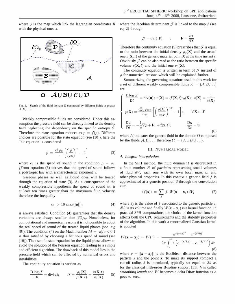
In the present work we model the Navier-Stokes equationsfor a set of viscous newtonian fluids. The sketch in figure (1)shows a fluid domainΩ composed by different fluidsA,B, . . ..The boundaries of the domainΩ are constituted by a free-surface∂ΩF and by solid boundaries∂ΩB.

The conservation of the momentum inΩ is written inlagrangian formalism as

DuDt

= −∇p

ρ+ Fv + FS + f (1)

whereu, p and ρ are respectively, the velocity, the pressureand the density fields, whilefV , fS , f represent the viscous, thesurface tension and the external body forces (here the forcefield ρf is the gravity forceρg).

The spatial position of the generic material pointX,at timet will be indicated throughx(t), in other words

x(t) = φ(X, t) (2)

3rd ERCOFTAC SPHERIC workshop on SPH applicationsJune,4th - 6th 2008, Lausanne, Switzerland

whereφ is the map which link the lagrangian coordinatesXwith the physical onesx.

Fig. 1. Sketch of the fluid-domainΩ composed by different fluids or phasesA,B, . . .).

Weakly compressible fluids are considered. Under this as-sumption the pressure field can be directly linked to the densityfield neglecting the dependency on the specific entropyS.Therefore the state equation reduces top = f(ρ). Differentchoices are possible for the state equation (see [10]), heretheTait equation is considered

p =c20 ρ0

γ

[(

ρ

ρ0

)γ

− 1

]

(3)

where c0 is the speed of sound in the conditionρ = ρ0.¿From equation (3) derives that the speed of sound followsa polytropic law with a characteristic exponentγ.

Gaseous phases as well as liquid ones will be treatedthrough the equation of state (3). As a consequence of theweakly compressible hypothesis the speed of soundc0 isat least ten times greater than the maximum fluid velocity,therefore the inequality

c0 > 10 max(|u|)Ω (4)

is always satisfied. Condition (4) guarantees that the densityvariations are always smaller than1%ρ0. Nonetheless, forcomputational and numerical reasons it is not possible to adoptthe real speed of sound of the treated liquid phases (seee.g[9]). The condition (4) on the Mach numberM = |u|/c < 0.1is thus satisfied by choosing a fictitious speed of sound (see[10]). The use of a state equation for the liquid phase allowstoavoid the solution of the Poisson equation leading to a simpleand efficient algorithm. The drawback of this model lies in thepressure field which can be affected by numerical errors andinstabilities.

The continuity equation is written as

D logJ

Dt= div(u); J =

ρ0(X)

ρ(X, t)=

v(X, t)

v0(X)(5)

where the Jacobian determinantJ is linked to the mapφ (seeeq. 2) through

J = det( F) ; F =∂x∂X

Therefore the continuity equation (5) prescribes thatJ is equalto the ratio between the initial densityρ0(X) and the actualoneρ(X, t) of the generic material pointX at the time instantt.ObviouslyJ can be also read as the ratio between the specificvolumev(X, t) and the initial onev0(X).

The continuity equation is written in term ofJ instead ofρ for numerical reasons which will be explained further.

Summarizing, the governing equations used in this work fora set of different weakly compressible fluidsX = (A,B, . . .)are

D logJ

Dt= div(u) ; v(X) = J (X, t)v0(X) ; ρ(X) =

1

v(X)

p(X) =c20X ρ0X

γX

[(

ρ(X)

ρ0X

)γX

− 1

]

; ∀X ∈ X

DuDt

= −1

ρ∇p + fV + f(x, t);

DxDt

= u

(6)whereX indicates the generic fluid in the domainΩ composedby the fluidsA,B, . . ., thereforeΩ = (A ∪ B ∪ . . .).

III. N UMERICAL MODEL

A. Integral interpolation

In the SPH method, the fluid domainΩ is discretized ina finite numberN of particles representing small volumesof fluid dV , each one with its own local massm andother physical properties. In this context a generic fieldf isapproximated at a generic position~x through the convolutionsum

〈f(x)〉 =∑

j

fj W (x − xj) dVj (7)

wherefj is the value off associated to the generic particlej,dVj is its volume and finallyW (x− xj) is a kernel function. Inpractical SPH computations, the choice of the kernel functionaffects both the CPU requirements and the stability propertiesof the algorithm. In this work a renormalized Gaussian kernelis adopted

W (x − xj) = W (r) =e−(r/h)2 − e−(δ/h)2

2π

∫ δ

0

r(

e−(r/h)2 − e−(δ/h)2)

dr

(8)where r = ‖x − xj‖ is the Euclidean distance between theparticle j and the pointx. To make its support compact acut-off radius δ is introduced, typically set equal to3h asfor the classical fifth-order B-spline support [11].h is calledsmoothing lengthandW becomes a delta Dirac function ashgoes to zero.


The spatial derivatives of the fieldf evaluated at the particlepositions can be estimated using the formula (7)

〈∇f(x)〉 =∑

j

(∇f)j W (x − xj) dVj . (9)

After some manipulation (see e.g. [9]) it is possible to movethe gradient operator to the kernel and the previous formulacan be approximated by

〈∇f(x)〉 = −∑

j

fj∇jW (x − xj)dVj

+ f(x)∑

j

∇jW (x − xj)dVj

(10)

where∇j denotes the derivative with respect toxj . The secondterm of equation (10) is practically zero far from the freesurface while it increases close to the free boundary; thereforethis term acts as a boundary term. Equation (10) can be simplyrearranged over the particle distribution as

〈∇f(xi)〉 =∑

j

(fj − fi)∇iW (xi − xj)dVj (11)

where the antisymmetric property of the kernel∇jW (xi −xj) = −∇iW (xi−xj) is used. Thanks to the difference(fj −fi) this formula is null for a constant field for any particledistribution as prescribed by equation (9).

B. SPH Formulations available in literature

1) Classical formulation:Considering a density field ap-proximated through the equation (7)

〈ρ(x)〉 =∑

j

ρj Wj(x) dVj (12)

if a direct relationship among the particle massmj , densityρj

and elementary volumedVj is assumed (i.e. ρj = mj/dVj ),the formula becomes

〈ρ(x)〉 =∑

j

mj Wj(x) (13)

where the density fieldρ is considered equal to thesmoothedfield 〈ρ〉. This formula allows an evaluation of the densityfield once the spatial distribution of the particle massesmj isknown.

Consistently, the associated discrete formula for the pressuregradient is

〈∇pi〉 = ρi

∑

j

(

pi

ρ2i

+pj

ρ2j

)

∇Wj(xi)mj (14)

2) Formulation for interface-flows with then − terms:A different approach has been used in the article by Hu &Adams [6] where, to overcome the limits of the formula (13),the density field is evaluated through

〈ρi〉 = mi ni ; ni =∑

j

Wj(xi) (15)

This formula is able to reproduce the density discontinuityinside the domainΩ. The density of generici-th particle is

not influenced by the massmj, nonetheless particlei receivesthe geometric contribution from particlej through Wj(xi).Note that the particlesi andj can belong to different phasesand, consequently, the densityρi does not degenerate close tothe interface. The termsni are purely geometrical since theyare only associated to the particle spatial distribution throughthe kernelW .

Consistently, the associated discrete formula for the pressuregradient is

〈∇pi〉 = ni

∑

j

(

pi

n2i

+pj

n2j

)

∇Wj(xi) (16)

The density representation given in (15) cannot be used iffree surfaces are present in the fluid domainΩ. In this case thedensity will unphysically vanish. Moreover, if particles havedifferent sizes the formula (15) can not take into account theirmass distribution. In fact, particlei has no information aboutthe masses of the neighbourhood particles and gives the samegeometric weight to each of them. Despite these limitationsthe formulation introduced by [6] does not require the timeintegration of the continuity equation. Such an approachguarantees the mass and volume conservation.

C. Present Formulation

In the present paper an SPH formulation based on the useof a Shepard kernel [1] for the density evaluation is presented.The Shepard kernel has been used in [3] to evaluate the forcesacting on the solid boundaries∂ΩB and to take into accountthe variation of the smoothing length,h, for problems char-acterized by strong compressibility. Here the solid boundariesare modelled through the ghost-particle technique, thereforethere is no need for evaluating the boundary forces explicitly.Further, a constant smoothing length is used all overΩ sinceonly weakly compressible effects are taken into account. TheShepard kernel is used here to model the presence of differentfluids. The present SPH formulation shows similarities withthe models derived in both [4] and [6].

The main idea of the present formulation is the followingdensity evaluation

〈ρ(x)〉 =∑

j∈Xmj WS

j (x) ; WSj (x) =

Wj(~x)

c(x);

c(x) =∑

k∈XWk(x) dVk ; ∀x ∈ X

(17)The Shepard kernelWS is normalized by definition andtherefore the identity

∑

j∈X

WSj (x) dVj = 1 ∀x ∈ X (18)

is always satisfied and does not depend on the number ofparticles.

The summation for calculating the termc(x) is extendedonly to the particles belonging to the fluid containing thepoint x. For this reason in (17) and in (18), the indices inthe summation are restricted to the particles belonging to thegeneric fluidX . In this way the discontinuities of the densityfield are treated explicitly.


Note that the density representation (17) is conceptuallydifferent from formula (13) since the Shepard kernelWS isfunction of the particle density distributiondV which hasto be calculated through the continuity equation (5). As aconsequence, the use of equation (17) leads to arelaxed linkbetween massmi, volumedVi and densityρi for the generici-th particle. Therefore the direct linkmi = ρi dVi will not beused anymore as discussed at the end of this section. On theother hand, if the volume distributiondV is evaluated througha geometrical tessellation of the domainΩ, the punctualratio mi/dVi can not coincide with the one obtained throughequations (13), (17) which only give asmoothedrepresentation〈ρ〉 of the density field (i.e. 〈ρ〉 < mi/dVi).

Summarizing, in the present formulation it is necessary totime integrate the continuity equation to evaluate the particlevolume distribution. Since the density is evaluated through theShepard kernel the divergence of the velocity is

〈div(ui)〉 =1

di

∑

j

(uj − ui) · ∇Wj(xi)dVj ;

d(x) =∑

k

Wk(x)dVk

(19)

where the summation is extended to all the particle neigh-bourhood without taking into account the different phases.In this way the discontinuities of the velocity field at theinterface will beregularizedby the equation (19). Conversely,as already stressed, the density discontinuities are explicitlytreated through equation (17).

Consistently, the new discrete formula for the smoothedpressure gradient is

〈∇pi〉 =∑

j

(

pi

di+

pj

dj

)

∇Wj(xi) dVj (20)

1) Introduction of the geometricaln− terms in the presentformulation: Similarly to the formulation proposed by Hu &Adams [6], it is possible to introduce thegeometricaltermsn(x) in the present formulation. The main difference is that theapproximation is done on the volume distribution instead ofon the particle masses (see equation (15)). As initial conditionfor all the simulations presented in this paper, particles arepositioned on a regular lattice and, consequently, their volumesare identical. Since we are working with weakly compressiblemedia, we assume that the volumesdVj of the particles closeto the generic particlei are almost identical todVi (i.e.spatial gradient of the volume distribution are negligibleonlength scale comparable to3h). Under this hypothesis, it ispossible to write that

Wj(xi) dVj

d(x)=

Wj(xi) dVj∑

k Wk(x) dVk≃

Wj(xi)∑

k Wk(x)=

Wj(xi)

n(x)(21)

Introducing this approximation into the divergence of the

velocity (19) and into the pressure gradient (20) we get

div(ui) =∑

j

(uj − ui) ·∇Wj(xi)

ni

∇pi =∑

j

(

pi

ni+

pj

nj

)

∇Wj(xi)(22)

In the previous equations, the influence of the particle volumeis no more present and is replaced by the geometrical termsn(x) as already highlighted for the equation (16).

Similarly to the approximation made for the termsd(x), afurther simplification can be applied toc(x)

ci =∑

k∈X

Wk(xi) dVk ≃ dVi

∑

k∈X

Wk(xi) = dVi li (23)

As a consequence, the density equation (17) can be rewrittenas

ρ(xi) =

∑

j∈XmjWj(xxi)

li dVi=

Mi

dVi

Mi =

∑

j∈XmjWj(xi)

∑

k∈XWk(xi)

(24)

This formula highlights that the densityρi and the volumedVi are related through asmootheddistribution of massMi

(which does not coincide with the punctual massmi).The geometrical termsl(x) are used for the evaluation of

M, while the continuity equation (5) is integrated in time forthe calculation of the volume distributiondV . Once the fieldsM anddV are known it is possible to evaluate the density fieldρ through equation (24) (and therefore the related pressurefield).

Summarizing the formulation proposed in this work dis-cretizes the continuum system of the governing equations (6)in the following way: at the generic time instantt positions,masses and volumes of the particles are known and, therefore,it is possible to evaluate the following quantities

Mi =

∑

j∈XmjWj(xi)

li; li =

∑

k∈X

Wk(xi)

ρi =Mi

dVi⇒ p(xi) =

c20Xρ0X

γX

[(

ρ(xi)

ρ0X

)γX

− 1

]

; ∀ xi ∈ X

(25)Once the updated density and pressure distributions are known,the fundamental derivatives can be evaluated by

Dxi

Dt= ui ; ni =

∑

k

Wk(xi)

D logJi

Dt=∑

j

(uj − ui) ·∇Wj(xi)

ni;

Dui

Dt= −

1

ρi

∑

j

(

pi

ni+

pj

nj

)

∇Wj(xi) + ~f(xi, t)

(26)Finally, using these derivatives it is possible to update volumes,velocities and positions of the particle set. Once again we un-derline that the present scheme allows to model both interfacesand free-surfaces (see figure 1). Note that if we consider onlyone fluid, it simply means thatli = ni.


2) Surface tension and viscous forces:Reagrding the sur-face tension and viscous forces, the work by [6] has beenconsidered adapting the formulae to the present formulation.A continuous surface force model (CSF) [8] has been adoptedto model the surface tension. To simplify the notation onlytwo phases (X ,Y) are considered. The surface tension forthe generici-th particle belonging to the phaseX due to thepresence ofY, can be evaluated by

FXY

Si= div(TXY

Si) ∀i ∈ X

TXY

Si= σXY 1

|∇CXY

Si|

(

1

d1|∇CXY

Si|2 −∇CXY

Si⊗∇CXY

Si

)

(27)whereFXY

Siis the surface-tension force acting on particlei,

TXY

Siis the surface stress tensor andσXY is the surface-tension

coefficient between the two phasesX andY; d is the spatialdimension of the problem. The tensorTXY

Sican be evaluated

through the spatial gradient of a color indexC which has aunit jump across the interface betweenX andY. In the presentformulation the∇CXY

i vector can be evaluated as,∀i ∈ X

CYi =

0 i ∈ X1 i ∈ Y

;∇CXYi =

∑

j∈Y

(

CYi

ni+

CYj

nj

)

∇Wj(xi)

(28)whereCY

i = 0 by definition since particlei belongs to phaseX . Note that this formulation provides surface tension effectsbetween two different phases but it does not produce anysurface tension on a free surface (where∇C becomes zero).Finally ,the divergence of the surface stress tensorTXY

Siis

evaluated through a discrete operator similar to the one usedfor the pressure gradient (see second equation 22 )

FXY

Si= div(TXY

Si) =

∑

j

TXY

Si

ni+

TXY

Sj

nj

∇Wj(xi)

(29)Following Flekkøy et al. [7], [6] the inter-particle-averaged

shear tensorTvij can be approximated as

Tvij =

2µiµj

µi + µj

1

r2ij

[

(xi−xj)⊗(ui−xj)+(xi−xj)⊗(xi−xj)

]

(30)whereµ is the viscosity coefficient related to the particle ofthe considered phase andrij is the distance between particlesi andj. The viscous forceFv acting on the generic particleican be evaluated through the discrete formula

Fvi =

∑

j

(

1

ni+

1

nj

)

Tvij ∇Wj(xi) (31)

If the viscous compressible effects can be neglected, thisformula can be rewritten as (for details see [6])

Fvi =

∑

j

2µiµj

µi + µj

(

1

ni+

1

nj

)

(xi − xj) · ∇Wj(xi)

r2ij

(vi − vj)

(32)which resembles a mixing of the formulae adopted by Morriset al. (see [13]) and Monaghan (see [12]) with the presence

of the new term[1/ni + 1/nj]. Differently from the equationproposed by Monaghan [12], (31) and (32) do not preservethe angular momentum. A possible generalization of theMonaghan formula can be

Fvi =

∑

j

19.8µi µj

µi + µj

(

1

ni+

1

nj

)

(xi − xj) · (vi − vj)

r2ij + ǫh2

∇Wj(xi)

(33)whereǫ ∼ 0.01 is introduced to prevent singularity wheni =j.

3) Control of interface sharpness:For interface flow wheresurface tension effects are negligible, a numerical dispersionof the different phases can take place. To prevent this mixinga small repulsive force is introduced in the pressure gradient

∇pi =∑

j

(

pi

ni+

pj

nj

)

∇Wj(xi)

+ ǫI

∑

j ∈XC

(∣

∣

∣

∣

pi

ni

∣

∣

∣

∣

+

∣

∣

∣

∣

pj

nj

∣

∣

∣

∣

)

∇Wj(xi) ∀i ∈ X

(34)whereǫI is of orderO(0.01÷ 0.1), and the second summationis extended to all the particles which do not belong to the phaseof the i-th particle; the latter set of particles is noted byXC .

IV. VALIDATION RESULTS

A. Rayleigh-Taylor instabilities

We consider the problem of Rayleigh-Taylor instabilitieswhere the interface between two different fluids needs to beaccurately calculated [5]. The computation domain is rectan-gular (twice as high as long) with particles distributed on aregular lattice. In the lower part of the domain, the fluid hasa density equal to unity while the fluid above the interfacelocated aty = 1 − sin(2πx) has got a density equal to 1.8times the density of the lower fluid. The Reynolds numberbased on the half-height of the domain is equal to 420. TheFroude number based on the same length scale is equal tounity. Surface tension is not taken into account. In the stateequationγ = 7 for both fluids.

Numerically, 28800 particles are used in the simulation. ThecoefficientǫI is equal to0.02. Space resolution convergencehas been checked.

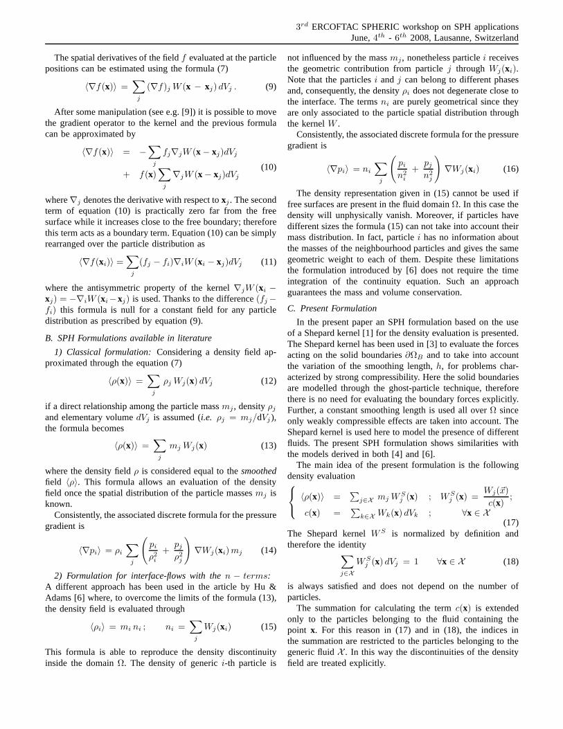
Results are compared to a Level-Set Navier-Stokes modelwith 28800 elements, see figure 2. The method shows a goodability to capture the strong roll-up of the interface.

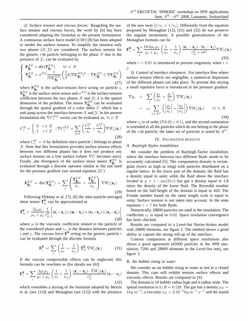
Contour comparison at different space resolutions alsoshows a good agreement (45000 particles in the SPH sim-ulation, 7200 and 28800 elements in the Level-Set one), seefigure 3.

B. Air bubble rising in water

We consider an air bubble rising in water at rest in a closeddomain. This case will exhibit tension surface effects andviscosity effects. Results are compared to [4].

The domain is 10 bubble radius high and 6 radius wide. Thespatial resolution ish/R = 0.128. The gas has a densityρX =1kg.m−3, a viscosityνX = 2.10−5kg.m−1.s−1 and the sound


0.5

0.5

1

1.5

2

0.5

0.5

1

1.5

2

x

y

SPH Level-Set

Fig. 2. Rayleigh-Taylor instabilities. Comparaison att = 5s versus a Level-Set model.

0.5 1

0.5

1

1.5

2t=4.456

0.5 1

0.5

1

1.5

2t=3.081

0.5 1

0.5

1

1.5

2t=1.046

Fig. 3. Rayleigh-Taylor instabilities. Comparaison at different times versusa Level-Set code. Gray contour corresponds to the heavier fluid modelizedby the present SPH model. Lines correspond to the interface of the Level-Setmodel on the coarse mesh (dashed line) and the fine mesh (solidline)

speed iscX = 282.84m.s−1. The liquid has a densityρY =1000kg.m−3, a viscosityνY = 1.10−3kg.m−1.s−1 and thesound speed iscY = 20m.s−1. The surface tension betweenthese two phases isσXY = 0.073N.m−1.

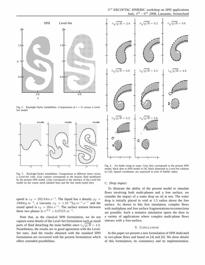
Note that, as the classical SPH formulation, we do notcapture some details of the Level-Set formulation such as smallparts of fluid detaching the main bubble sincet

√

g/R = 4.8.Nonetheless, the results are in good agreement with the Level-Set ones. And the results obtained with the standard SPHformulation are recovered with the present formulation whichoffers extended possibilities.

t√

g/R = 2.8 t√

g/R = 3.2 t√

g/R = 3.6

t√

g/R = 4.0 t√

g/R = 4.4 t√

g/R = 4.8

t√

g/R = 5.2 t√

g/R = 5.6

Fig. 4. Air buble rising in water. Gray dots corresponds to the present SPHmodel, black dots to SPH model in [4], black diamonds to Level-Set solutionin [14]. Spatial coordinates are expressed in term of bubbleradius

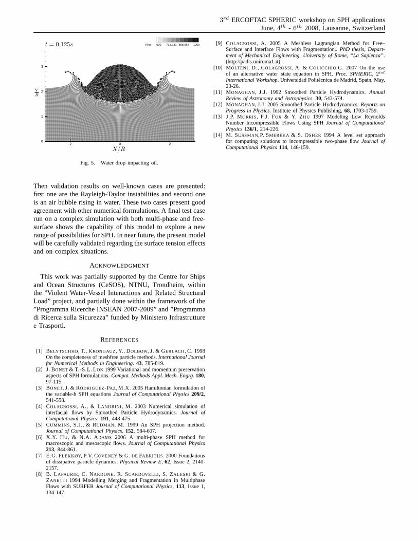
C. Drop impact

To illustrate the ability of the present model to simulateflows involving both multi-phases and a free surface, weconsider the impact of a water drop on oil at rest. The waterdrop is initially placed in void at 1.5 radius above the freesurface. As shown in this first simulation, complex flowswith multiphase and free surface fragmentations/reconnectionsare possible. Such a tentative simulation opens the door toa variety of applications where complex multi-phase flowsinteract with a free-surface.

V. CONCLUSION

In this paper we present a new formulation of SPH dedicatedto two-phase flows and based on [4] and [6]. We show detailsof this formulation, its consistency and its implementation.


-2 0 20

1

2

3

Rho: 600 733.333 866.667 1000

X/R

Y

R

t = 0.125s

Fig. 5. Water drop impacting oil.

Then validation results on well-known cases are presented:first one are the Rayleigh-Taylor instabilities and second oneis an air bubble rising in water. These two cases present goodagreement with other numerical formulations. A final test caserun on a complex simulation with both multi-phase and free-surface shows the capability of this model to explore a newrange of possibilities for SPH. In near future, the present modelwill be carefully validated regarding the surface tension effectsand on complex situations.

ACKNOWLEDGMENT

This work was partially supported by the Centre for Shipsand Ocean Structures (CeSOS), NTNU, Trondheim, withinthe ”Violent Water-Vessel Interactions and Related StructuralLoad” project, and partially done within the framework of the”Programma Ricerche INSEAN 2007-2009” and ”Programmadi Ricerca sulla Sicurezza” funded by Ministero Infrastrutturee Trasporti.

REFERENCES

[1] BELYTSCHKO, T., KRONGAUZ, Y., DOLBOW, J. & GERLACH, C. 1998On the completeness of meshfree particle methods.International Journalfor Numerical Methods in Engineering. 43, 785-819.

[2] J. BONET & T.-S.L. LOK 1999 Variational and momentum preservationaspects of SPH formulations.Comput. Methods Appl. Mech. Engrg.180,97-115.

[3] BONET, J. & RODRIGUEZ-PAZ , M.X. 2005 Hamiltonian formulation ofthe variable-h SPH equationsJournal of Computational Physics209/2,541-558.

[4] COLAGROSSI, A., & L ANDRINI , M. 2003 Numerical simulation ofinterfacial flows by Smoothed Particle Hydrodynamics.Journal ofComputational Physics. 191, 448-475.

[5] CUMMINS , S.J., & RUDMAN , M. 1999 An SPH projection method.Journal of Computational Physics. 152, 584-607.

[6] X.Y. H U, & N.A. A DAMS 2006 A multi-phase SPH method formacroscopic and mesoscopic flows.Journal of Computational Physics213, 844-861.

[7] E.G. FLEKKØY, P.V. COVENEY & G. DE FABRITIIS . 2000 Foundationsof dissipative particle dynamics.Physical Review E, 62, Issue 2, 2140-2157.

[8] B. L AFAURIE, C. NARDONE, R. SCARDOVELLI , S. ZALESKI & G.ZANETTI 1994 Modelling Merging and Fragmentation in MultiphaseFlows with SURFERJournal of Computational Physics, 113, Issue 1,134-147

[9] COLAGROSSI, A. 2005 A Meshless Lagrangian Method for Free–Surface and Interface Flows with Fragmentation..PhD thesis, Depart-ment of Mechanical Engineering, University of Rome, “La Sapienza”.(http://padis.uniroma1.it).

[10] MOLTENI, D., COLAGROSSI, A. & COLICCHIO G. 2007 On the useof an alternative water state equation in SPH.Proc. SPHERIC,2nd

International Workshop. Universidad Politecnica de Madrid, Spain, May,23-26.

[11] MONAGHAN, J.J. 1992 Smoothed Particle Hydrodynamics.AnnualReview of Astronomy and Astrophysics. 30, 543-574.

[12] MONAGHAN, J.J. 2005 Smoothed Particle Hydrodynamics.Reports onProgress in Physics. Institute of Physics Publishing,68, 1703-1759.

[13] J.P. MORRIS, P.J. FOX & Y. Z HU 1997 Modeling Low ReynoldsNumber Incompressible Flows Using SPHJournal of ComputationalPhysics136/1, 214-226.

[14] M. SUSSMAN,P. SMEREKA & S. OSHER 1994 A level set approachfor computing solutions to incompressible two-phase flowJournal ofComputational Physics114, 146-159.

Simulation of Interfacial and Free-Surface Flows using a new SPH formulation

Documents

Transcript of Simulation of Interfacial and Free-Surface Flows using a new SPH formulation