This article was downloaded by:[ANKOS Consortium]On: 18 January 2008Access Details: [subscription number 772815469]Publisher: Taylor & FrancisInforma Ltd Registered in England and Wales Registered Number: 1072954Registered office: Mortimer House, 37-41 Mortimer Street, London W1T 3JH, UK

Numerical Heat Transfer, Part B:FundamentalsAn International Journal of Computation andMethodologyPublication details, including instructions for authors and subscription information:http://www.informaworld.com/smpp/title~content=t713723316

Modeling Transient Heat Transfer Using SPH andImplicit Time IntegrationRusty Rook a; Mehmet Yildiz a; Sadik Dost aa Crystal Growth Lab, Department of Mechanical Engineering, University of Victoria,Victoria, British Columbia, Canada

Online Publication Date: 01 January 2007To cite this Article: Rook, Rusty, Yildiz, Mehmet and Dost, Sadik (2007) 'Modeling

Transient Heat Transfer Using SPH and Implicit Time Integration', Numerical Heat Transfer, Part B: Fundamentals, 51:1,1 - 23To link to this article: DOI: 10.1080/10407790600762763URL: http://dx.doi.org/10.1080/10407790600762763

PLEASE SCROLL DOWN FOR ARTICLE

Full terms and conditions of use: http://www.informaworld.com/terms-and-conditions-of-access.pdf

This article maybe used for research, teaching and private study purposes. Any substantial or systematic reproduction,re-distribution, re-selling, loan or sub-licensing, systematic supply or distribution in any form to anyone is expresslyforbidden.

The publisher does not give any warranty express or implied or make any representation that the contents will becomplete or accurate or up to date. The accuracy of any instructions, formulae and drug doses should beindependently verified with primary sources. The publisher shall not be liable for any loss, actions, claims, proceedings,demand or costs or damages whatsoever or howsoever caused arising directly or indirectly in connection with orarising out of the use of this material.

Dow

nloa

ded

By:

[AN

KO

S C

onso

rtium

] At:

10:1

5 18

Jan

uary

200

8

MODELING TRANSIENT HEAT TRANSFER USING SPHAND IMPLICIT TIME INTEGRATION

Rusty Rook, Mehmet Yildiz, and Sadik DostCrystal Growth Lab, Department of Mechanical Engineering, University ofVictoria, Victoria, British Columbia, Canada

In this article, a two-dimensional transient heat conduction problem is modeled using

smoothed particle hydrodynamics (SPH) with a Crank-Nicolson implicit time integration

technique. The main feature of this work is that it applies implicit time stepping, an uncon-

ditionally stable Crank-Nicolson approach, in the thermal conduction simulation of liquid-

phase diffusion (LPD) semiconductor crystal growth. This SPH simulation is compared

with the equivalent finite-volume results. As well, two transient thermal conduction test pro-

blems are simulated using both explicit and Crank-Nicolson schemes, and their results com-

pared with the analytical solutions. One of the current drawbacks of SPH is that explicit

time-stepping algorithms, such as predictor-corrector methods or leapfrog methods, require

extremely small time steps for a stable simulation. Using implicit time integration opens

SPH up to a much larger class of practical problems in applied mechanics.

1. INTRODUCTION

Smoothed particle hydrodynamics (SPH) is an adaptive, mesh-free, Lagrangiannumerical approximation technique used for modeling physical problems. UnlikeEulerian computational techniques such as the finite-volume and finite-differencemethods, SPH does not require a grid, as derivatives are approximated using a kernelfunction. Each ‘‘particle’’ in the domain can be associated with one discrete physicalobject, or it may represent a macroscopic part of the continuum [1]. The continuum isrepresented by an ensemble of particles each carrying mass, momentum, and otherhydrodynamic properties. In recent years, several other mesh-free methods have beengaining popularity in the literature, such as the meshless element-free Galerkin (EFG)method [2–5], moving least-square methods [6], or the diffuse approximation method[7]. However, these approaches tend to be formulated in a Eulerian frame. TheLagrangian framework of SPH is convenient for simulations involving interfacialsurfaces, such as in the field of semiconductor crystal growth. For this application,the finite-volume approach is difficult to implement, as the computational mesh isrequired to adapt to the crystal growth surface. Although originally proposed tohandle cosmological simulations [8, 9], SPH has become increasingly generalized to

Received 8 November 2005; accepted 31 March 2006.

Funding provided by the Natural Sciences and Engineering Research Council and the Canada

Research Chairs is greatfully acknowledged.

Address correspondence to Sadik Dost, Crystal Growth Lab, Department of Mechanical Engineer-

ing, University of Victoria, Victoria, BC V8W 3P6, Canada. E-mail: sdost@me.uvic.ca

1

Numerical Heat Transfer, Part B, 51: 1–23, 2007

Copyright # Taylor & Francis Group, LLC

ISSN: 1040-7790 print=1521-0626 online

DOI: 10.1080/10407790600762763

Dow

nloa

ded

By:

[AN

KO

S C

onso

rtium

] At:

10:1

5 18

Jan

uary

200

8

handle many types of fluid and solid mechanics problems [10–13]. SPH advantagesinclude relatively easy modeling of complex material surface behavior, as well as sim-ple implementation of more complicated physics, such as solidification [14].

In many applications, such as crystal growth [15–17], systems must be simu-lated as they evolve over a period of several minutes or hours. A review of SPHliterature reveals that SPH has not yet been applied to solve practical problemsinvolving large time scales. The explicit-time-step algorithms currently used inSPH simulations require miniscule time steps for a stable solution, putting theSPH method out of reach for many computational fluid dynamics (CFD) problems.If implicit time stepping was incorporated in SPH, the range of applicability wouldgreatly increase. Other sources in the literature have encorporated implicit and semi-implicit time integration [18], but to our knowledge it has not yet been investigated incrystal growth applications.

The SPH technique computes discrete particle properties using a smoothing,kernel distribution function to account for the effects of surrounding particles. Itis assumed that the properties characteristic of the particle of interest are influencedby all other particles in the global domain. However, one approximation of SPH is toinclude only the effects of nearby particles, within a smoothing radius denoted 2h.The length h defines the support domain of the particle of interest (i.e., a localizeddomain over which the kernel will be nonzero). Throughout the present simulations,the compactly supported cubic spline kernel

Wðxij; hÞ ¼ an

23�

xij

h

� �2þ 12

xij

h

� �3if 0 � xij < h

16 2� xij

h

� �3� �

if h � xij < 2h

0 if xij � 2h

8><>: ð1Þ

NOMENCLATURE

an kernel dimension coefficients

Aij interaction coefficient

ci speed of sound for particle i

cp specific heat capacity

CCFL Courant coefficient

f ðxbi Þ arbitrary position function

hf ðxbi Þi SPH approximation of f ðxb

i Þg determinant of gab

gab metric tensor

h, hij smoothing length

H domain height

H convective heat transfer coef.

H modified heat transfer coef.

L domain length

mi mass of particle i

N total number of particles

R radius

t time

Dt time increment

T temperature

Tf ambient furnace temperature

Wðxij ; hÞ kernel function

xai position vector of i

xaij positional difference

xij magnitude of xaij

ðx; y; zÞ Cartesian coord.

aD diffusivity

bk series coefficient

cl series coefficient

d3ðxbijÞ 3-D Kronecker delta

j conductivity

jS solid conductivity

q density

Subscripts

i; j particle indices

0 reference state

Superscripts

m time-step index

a; b; c;k component indices

2 R. ROOK ET AL.

Dow

nloa

ded

By:

[AN

KO

S C

onso

rtium

] At:

10:1

5 18

Jan

uary

200

8 was employed, where xij is the magnitude of the distance between particles i and j. InEq. (1), n is the dimension of the space, and the coefficient an is dependent on thesmoothing length h and has values

a1 ¼1

ha2 ¼

15

7ph2a3 ¼

3

2ph3

in one, two, and three dimensions, respectively. For h ¼ 1, the cubic spline kerneldisribution of Eq. (1) is illustrated for a two-dimensional (x1

ij ; x2ij) Cartesian domain

in Figure 1.For clarity, it is worthwhile taking a moment to state explicitly the notational

conventions that will be used throughout this article. All vector quantities will bewritten using the index notation, with Greek indices denoting the tensor componentsexclusively. These components will always be written in contravariant form as super-scripts. As well, throughout this article, the Einstein summation convention isemployed, where any repeated index is summed over the range of the index. Latinindices (i; j) will be used to denote particles, and will always be placed as subscripts.For example, the n-dimensional vector denoting the position of particle i is written as

x!i ! xai for a ¼ 1; 2; . . . ; n ð2Þ

As well, we will employ the concise ð Þij difference notation,

xaij � xa

i � xaj where xij � xa

i � xaj

��� ��� ¼ ffiffiffiffiffiffiffiffiffiffiffiffiffiffiffiffiffigabxa

ijxbij

q

is the magnitude of the distance between particles i and j written in a curvilinearcoordinate system in terms of the metric tensor gab.

Figure 1. A 2-D cubic spline kernel.

TRANSIENT HEAT TRANSFER USING SPH 3

Dow

nloa

ded

By:

[AN

KO

S C

onso

rtium

] At:

10:1

5 18

Jan

uary

200

8 For two-dimensional thermal conduction in Cartesian coordinates, the govern-ing equation for the evolution of the temperature field T ¼ Tðx; y; tÞ is

qcpqT

qt¼ jgabT;ab )

qT

qt¼ aD �

q2T

qx2þ q2T

qy2

!ð3Þ

where cp is the specific heat, j is the (constant) thermal conductivity, q is thematerial density, and aD ¼ j=qcp is the thermal diffusivity. The quantity gabT;ab isthe Laplacian of the temperature field in general curvilinear coordinates interms of the second covariant derivative operator ð Þ;ab and the conjugate metrictensor gab.

2. SMOOTHED PARTICLE HYDRODYNAMICS

The three-dimensional Dirac delta function d3ðxbijÞ is the starting point for the

SPH approximation technique. This function satisfies the identity

f ðxbi Þ ¼

Z Z ZX

f ðxbj Þd3ðxb

ijÞdX ð4Þ

where dX ¼ ffiffiffigp

dx1dx2dx3 ¼ ffiffiffigp

dxb is a differential volume element. The fundamen-tal approximation of SPH is to replace the Dirac delta function with the even kernelfunction Wðxij; hÞ. We then write the fundamental SPH approximation in threedimensions as

f ðxbi Þ � hf ðx

bi Þi �

Z Z ZX

f ðxbj ÞWðxij ; hÞdX ð5Þ

where hf ðxbi Þi is the kernel approximation of the scalar field f ðxb

i Þ at particle i.

2.1. Spatial Derivatives in SPH

Since SPH is an approximation technique, there are several different ways ofapproximating spatial derivatives. In this section, we present SPH approximationsfor the gradient of a scalar function, and the Laplacian of a scalar function.

In order to determine the SPH approximation for the gradient of a scalar func-tion, we make the substitution f ðxb

j Þ ! f;ajðxb

j Þ in Eq. (5) to produce

hf;aðxbi Þi ¼

Z Z ZX

f;ajðxb

j ÞWðxij; hÞdX

where the covariant differentiations takes place referencing xbi coordinates using the

ð Þ;a operator, and xbj coordinates using the ð Þ;aj

operator. Upon integrating by

4 R. ROOK ET AL.

Dow

nloa

ded

By:

[AN

KO

S C

onso

rtium

] At:

10:1

5 18

Jan

uary

200

8 parts, and noting that W;aðxij ; hÞ ¼ �W;ajðxij; hÞ, it can be shown that

hf;aðxbi Þi ¼

Z Z ZX

f ðxbj ÞW;aðxij ; hÞdX ð6Þ

for all interior particles i. In the present article, the error introduced by the kerneltruncation of near-boundary interior particles has been neglected. This result isespecially significant, since it states that the spatial derivatives of particle propertiescan be found simply by differentiation of the kernel.

The SPH Laplacian of a scalar field f;ckðxbi Þ is derived in the Appendix, and is

given as

hgckf;ckðxbi Þi ¼ 2

Z Z ZX

f ðxbi Þ � f ðxb

j Þh i

xaij

gmnxmijx

nij

W;aðxij ; hÞdX ð7Þ

in terms of the gradient of the kernel, where all covariant derivatives in the aboveequation are with respect to xb

i coordinates.

2.2. Particle Approximations in SPH

Recall that Eq. (5) is the SPH approximation for a continuous distribution. If,however, we recognize that this integration will be carried out over all N discrete par-ticles within the domain, we can discretize Eq. (5) as

hf ðxbi Þi ¼

XN

j¼1

mj

qj

f ðxbj ÞWðxij ; hÞ ð8Þ

to produce the SPH approximation of a field property f ðxbÞ at particle i in terms ofall other interacting particles j, and a representative particle volume written in termsof particle mass mj and particle density qj.

In the following simulations, the discrete SPH particle appoximation used forthe gradient of a scalar function is

hf;aðxbi Þi ¼

XN

j¼1

mj

qi

f ðxbj Þ � f ðxb

i Þh i

W;aðxij; hÞ ð9Þ

The discrete form of the SPH approximation for the Laplacian of a scalar function iswritten from discretization of Eq. (7) as

hgckf;ckðxbi Þi ¼ 2

XN

j¼1

mj

qj

½f ðxbi Þ � f ðxb

j Þ�xij

qWðxij ; hÞqxij

ð10Þ

TRANSIENT HEAT TRANSFER USING SPH 5

Dow

nloa

ded

By:

[AN

KO

S C

onso

rtium

] At:

10:1

5 18

Jan

uary

200

8 3. EXPLICIT AND IMPLICIT TIME-STEPPING USING THE CRANK-NICOLSONALGORITHM

In order to increment the time step Dt in a numerical simulation, one can useeither an explicit or an implicit scheme.

3.1. Explicit Time Stepping

Explicit schemes are the most straightforward to apply, but are notoriouslysusceptible to instabilities when Dt becomes too great. For example, the time discre-tization of Eq. (3) using the most straightforward explicit approach is

Tmþ1i � Tm

i

Dt¼ 2aDi

XN

j¼1

j 6¼i

mj

qj

ðTmi � Tm

j Þxij

qWðxij ; hÞqxij

where we have used Eq. (10) for the SPH approximation for the Laplacian of thetemperature field, and the superscript m denotes the time step. Rearranging theabove equation, we have that

Tmþ1i ¼ Tm

i þ 2aDi DtXN

j¼1

j 6¼i

mj

qj

ðTmi � Tm

j Þxij

qWðxij; hÞqxij

ð11Þ

which is an SPH equation used to solve for the temperature distribution at thediscrete time step mþ 1. In three-dimensional simulations, the quantity mj=qj repre-sents the particle volume. However, for the two-dimensional problems considered,this quantity is interpreted as a characteristic particle area. Since the particles areequally spaced, the particle area is approximated by dividing the domain area bythe number of particles. Monaghan and Cleary have reported [19] that for pureconduction problems, the time step for an explicit scheme must satisfy

Dt � 0:15h2

aDð12Þ

for a stable solution. Since in the following simulations we have taken h ¼ 0:25 cmand aD ¼ 1 cm2=s, the time step is restricted to Dt � 0:009 s to ensure an accuratesolution.

In more complicated models where particles move, the explicit leapfrogalgorithm [20] can be used to break down the thermomechanical balance laws (con-servation of mass, momentum, and energy) into discrete time steps. The algorithmstability is controlled by the Courant-Friedrichs-Lewy (CFL) condition, where therecommended time step is

Dt � CCFLh

maxðci þ vai

�� ��Þ ð13Þ

6 R. ROOK ET AL.

Dow

nloa

ded

By:

[AN

KO

S C

onso

rtium

] At:

10:1

5 18

Jan

uary

200

8 where CCFL is a constant between 0 and 1, vai is the particle velocity, and ci is the

speed of sound for the particle material. The CFL condition is a major drawbackof using an explicit-time-step approach, as Dt is usually required to be extremelysmall. This fact makes the leapfrog technique well suited to problems involving onlyvery small time scales. However, for simulations involving large time scales, explicitapproaches such as the leapfrog technique are not suitable.

3.2. Implicit Crank-Nicolson Time Stepping

It is well known that implicit time-stepping approaches, such as the Crank-Nicolson approach, are unconditionally stable with respect to choice of Dt. Usinga simple implicit approach, Eq. (11) has the right-hand side modified to read

Tmþ1i ¼ Tm

i þ 2aDi DtXN

j¼1

j 6¼i

mj

qj

ðTmþ1i � Tmþ1

j Þxij

qWðxij; hijÞqxij

ð14Þ

where now there is no longer an explicit equation for the temperature of particle i attime step mþ 1. Instead of solving systematically for each temperature Tmþ1

i as wasdone in the explicit scheme, with the implicit approach we must now solve the systemof equations

Tmþ1i 1�

XN

j¼1

j 6¼i

Aij

2664

3775þX

N

j¼1

j 6¼i

AijTmþ1j ¼ Tm

i ð15Þ

where

Aij � 2aDi Dtmj

qj

1

xij

qWðxij; hijÞqxij

ð16Þ

is a dimensionless parameter characterizing the relationship between particles i and j.Here, at each time step mþ 1, a matrix must be inverted.

Alternatively, the Crank-Nicolson implicit technique is described by

Tmþ1i ¼ Tm

i þ aDi DtXN

j¼1

j 6¼i

mj

qj

ðTmþ1i � Tmþ1

j Þxij

qWðxij; hijÞqxij

þ aDi DtXN

j¼1

j 6¼i

mj

qj

ðTmi � Tm

j Þxij

qWðxij ; hijÞqxij

ð17Þ

This system of equations is rewritten and solved in the form

Tmþ1i 1�

XN

j¼1

j 6¼i

Aij

2

2664

3775þX

N

j¼1

j 6¼i

Aij

2Tmþ1

j ¼ Tmi 1þ

XN

j¼1

j 6¼i

Aij

2

2664

3775�X

N

j¼1

j 6¼i

Aij

2Tm

j ð18Þ

TRANSIENT HEAT TRANSFER USING SPH 7

Dow

nloa

ded

By:

[AN

KO

S C

onso

rtium

] At:

10:1

5 18

Jan

uary

200

8 where Aij is defined from Eq. (16). Equation (18) gives the Crank-Nicolsonsolution to the temperature of a given particle i at time mþ 1. The unknowntemperatures Tmþ1

i and Tmþ1j (consisting of all j neighboring particles of i) have

been grouped to the left-hand side of Eq. (18). All quantities on the right-hand sideare known, since the particle temperatures at time step m are determined. There-fore, for a total number of particles N, Eq. (18) produces i ¼ 1; 2; . . . ;N equationsfor N unknowns. Since N is typically much greater than the number of particleneighbors for a given particle of interest i, this system of equations will containmostly zeros, forming a sparse system. Several algorithms exist for the solutionof the above system of equations, such as direct matrix inversion, Gauss-Siedeliteration, or the biconjugate gradient method. In terms of solution approaches,the biconjugate gradient method was found to outperform Gauss-Siedel iterationand direct matrix inversion in terms of convergence and efficiency. Further detailson this approach can be found in the literature [21] and are discussed in thefollowing section.

Note that for general CFD problems, the SPH particles will move, and boththe distance between particles xij and the kernel derivatives qW=qxij will requirecomputation at time steps m and mþ 1, respectively. Indeed, the particle interactionsmake implementation of implicit time stepping more complicated in terms of solu-tions of the general Navier–Stokes equations.

For simulations involving static particles, however, like those in the presentwork, no distinction between time steps is required since particle positions do notevolve. Liquid-phase diffusion (LPD) semiconductor crystal growth is one suchapplication, where a low Prandtl number for the system allows computation ofthe thermal field independent from the flow field.

Monaghan suggested [18] a pairwise implicit time-marching scheme for thetreatment of a multiphase continuum such as a mixture of dust and gas. Inthis work, he resolved the coupling between the separate equations of motionfor the dust and the gas by considering each interacting pair separately, rather thanincluding contributions from all neighbor particles for the particle of interest. Hispairwise approach is contrasted with the direct implicit method applied in thepresent work. For multiphase continua, the pairwise approach is advantageousover a direct implicit scheme, which will require solution of matrices with bandswith a size about the number of the neighbor particles. However, if the pairwiseinteraction is utilized for the solution of the balance of momentum for asingle-phase continuum, it is equivalent to direct implicit time integration, as inves-tigated here.

4. TRANSIENT CONDUCTION MODELING

Two thermal conduction problems were solved and compared with knownanalytical solutions, set in a two-dimensional Cartesian domain 0 � x � L and0 � y � H, where L ¼ H ¼ 10 cm was selected. This ðx; yÞ problem domainwas modeled with SPH using N ¼ 1;600 (a grid of 40� 40) particles shown inFigure 2. Boundary particles are designated with the symbol, whereas interiorparticles use the symbol.

8 R. ROOK ET AL.

Dow

nloa

ded

By:

[AN

KO

S C

onso

rtium

] At:

10:1

5 18

Jan

uary

200

8

4.1. 2-D Transient Heat Conduction Problem 1

The first problem was to model the temperature profile Tðx; y; tÞ of the coolingof a plate at select times t. The plate was subjected to the boundary conditions

Tðx; 0; tÞ ¼ Tðx;H; tÞ ¼ Tð0; y; tÞ ¼ TðL; y; tÞ ¼ T1

and the initial condition

Tðx; y; 0Þ ¼ T0

where T0 is a uniform initial temperature throughout the domain. This domain isillustrated in the schematic in Figure 3.

For this simulation we use Eq. (3) and take the parameter values aD ¼ 1cm2=s,T0 ¼ 100; and T1 ¼ 0C. By separating variables, and applying the given boundaryand initial conditions, an analytical solution to the temperature field Tðx; y; tÞ can bedetermined and given in terms of the double infinite series

Tðx; y; tÞ ¼ 16T0

p2

X1k¼1;3;...

X1l¼1;3;...

exp �aDp2 k2=L2 þ l2=H2� �

t� �

klsin

kpx

L

sin

lpy

H

ð19Þ

Figure 4 illustrates the isothermal plots at times t ¼ 0:25, t ¼ 1, t ¼ 4, and t ¼ 8 sobtained from the analytical solution of Eq. (19) and the explicit time integrationequation (11), where T0 ¼ 100 and T1 ¼ 0C. The SPH solution is represented bythe dotted lines, and the analytical series solution by the solid lines. For the chosendomain of N ¼ 1;600 particles, the representative particle area is found asmj=qj ’ 0:0625 cm2, for L ¼ H ¼ 10 cm. The SPH solution correlates very well with

Figure 2. SPH test problem domain for N ¼ 1;600 particles.

TRANSIENT HEAT TRANSFER USING SPH 9

Dow

nloa

ded

By:

[AN

KO

S C

onso

rtium

] At:

10:1

5 18

Jan

uary

200

8

the known analytical solution for a smoothing length of h ¼ 0:25 cm, N ¼ 1;600particles, and Dt ¼ 0:009 s.

As expected, the explicit solution illustrated in Figure 4 was observed to breakdown as Dt was increased, in accordance with Eq. (12). However, the unconditionalstability of the implicit time integration schemes permitted larger time steps, whilethe solution accuracy was maintained. It was found that the time step could be

Figure 3. A 2-D ðx; yÞ spatial domain with temperature boundary and initial conditions.

Figure 4. Analytical and explicit SPH isothermal contours at times t ¼ 0:25, t ¼ 1, t ¼ 4, and t ¼ 8 s found

from Eqs. (19) and (11).

10 R. ROOK ET AL.

Dow

nloa

ded

By:

[AN

KO

S C

onso

rtium

] At:

10:1

5 18

Jan

uary

200

8 approximately doubled for the implicit schemes. A further increase in time stepcaused a significant reduction in solution accuracy.

Simulations to t ¼ 8 s using the implicit equation (15) and Dt ¼ 0:25 s tookapproximately 87 s of CPU time on a 64-bit AMD 3500þ processor, and the resultsare shown in Figure 5. These results correlate well with the explicit solution obtainedin Figure 4.

4.2. 2-D Transient Heat Conduction Problem 2

The second simulation involved transient heat conduction with more compli-cated boundary conditions. Once again, the rectangular domain 0 � x � L and0 � y � H was heated to an initial uniform temperature of Tðx; y; 0Þ ¼ T0 withtwo insulated boundaries

qTð0; y; tÞqx

¼ 0qTðx; 0; tÞ

qy¼ 0

Figure 5. Analytical and implicit SPH isothermal contours at times t ¼ 0:25, t ¼ 1, t ¼ 4, and t ¼ 8 s

found from Eqs. (19) and (15).

TRANSIENT HEAT TRANSFER USING SPH 11

Dow

nloa

ded

By:

[AN

KO

S C

onso

rtium

] At:

10:1

5 18

Jan

uary

200

8 and two boundaries that dissipate heat by convection to a medium at zerotemperature,

qTðL; y; tÞqx

¼ �Hj

TðL; y; tÞ qTðx;H; tÞqy

¼ �Hj

Tðx;H; tÞ

where H is the convective heat transfer coefficient. These boundary conditions areillustrated in Figure 6.

Using the above mixed boundary conditions, the analytical solution to Eq. (3)for this problem can be shown to be [22]

Tðx; y; tÞ ¼ 4T0

X1k¼1

X1l¼1

H2exp �aD b2

k þ c2l

� �t

� �cosðbkxÞ cosðclyÞ

Lðb2k þH

2Þ þ Hh i

Hðc2l þH

2Þ þ Hh i

cosðbkLÞ cosðclHÞ

ð20Þ

where H ¼ H=j, and bk and cl are the positive roots to the transcendental equations

bk tanðbkLÞ ¼ Hj

and cl tanðclHÞ ¼Hj

ð21Þ

In the following simulation, we take aD ¼ 1cm2=s; j ¼ 1 W=cm K; andH ¼ 0:1 W=cm2 K for the diffusivity, conductivity and convective heat transfer coef-ficient, respectively, as well as T0 ¼ 100C.

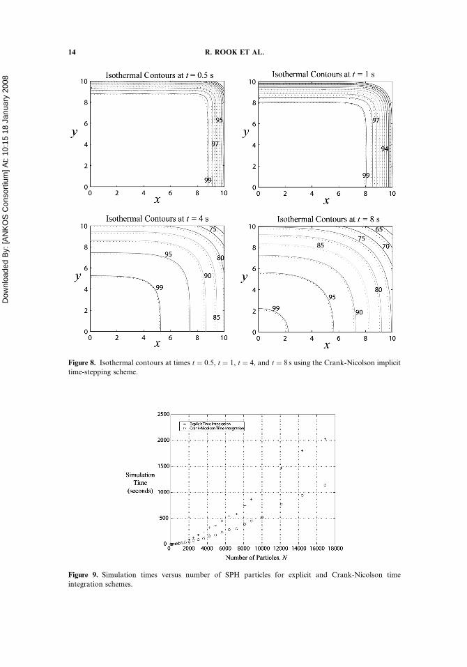
The evolution of the temperature profile according to Eq. (20) is plotted inFigure 7 for times t ¼ 0:5, t ¼ 1, t ¼ 4, and t ¼ 8 s. As before, the SPH governingheat transfer equation is expressed implicitly by Eq. (18). The SPH boundaryconditions were written using Eq. (9) for the boundary temperature gradients, wherea factor of 2 was added to balance the one-sided nature of the gradient at the bound-ary. Written explicitly for each boundary surface in Cartesian coordinates, we obtain

Figure 6. A 2-D ðx; yÞ spatial domain with temperature boundary and initial conditions.

12 R. ROOK ET AL.

Dow

nloa

ded

By:

[AN

KO

S C

onso

rtium

] At:

10:1

5 18

Jan

uary

200

8

the boundary conditions that must be satisfied for all time as

qTið0; y; tÞqx

� �¼XN

j¼1j 6¼i

2mj

qi

ðTj � TiÞqWðxij ; hijÞ

qxi¼ 0

qTiðx; 0; tÞqy

� �¼XN

j¼1j 6¼i

2mj

qi

ðTj � TiÞqWðxij ; hijÞ

qyi¼ 0

and

qTiðL; y; tÞqx

� �¼XN

j¼1j 6¼i

2mj

qi

ðTj � TiÞqWðxij; hijÞ

qxi¼ �H

jTiðL; y; tÞ

qTiðx;H; tÞqy

� �¼XN

j¼1j 6¼i

2mj

qi

ðTj � TiÞqWðxij; hijÞ

qyi¼ �H

jTiðx;H; tÞ

where in this case i is the boundary particle of interest.Using the implicit Crank-Nicolson approach, the SPH temperature contours

were found up to a time of t ¼ 8 s, and are given along with the analytical solution

Figure 7. Analytical temperature profile at times t ¼ 0:5, t ¼ 1, t ¼ 4, and t ¼ 8 s found from Eq. (20).

TRANSIENT HEAT TRANSFER USING SPH 13

Dow

nloa

ded

By:

[AN

KO

S C

onso

rtium

] At:

10:1

5 18

Jan

uary

200

8

Figure 8. Isothermal contours at times t ¼ 0:5, t ¼ 1, t ¼ 4, and t ¼ 8 s using the Crank-Nicolson implicit

time-stepping scheme.

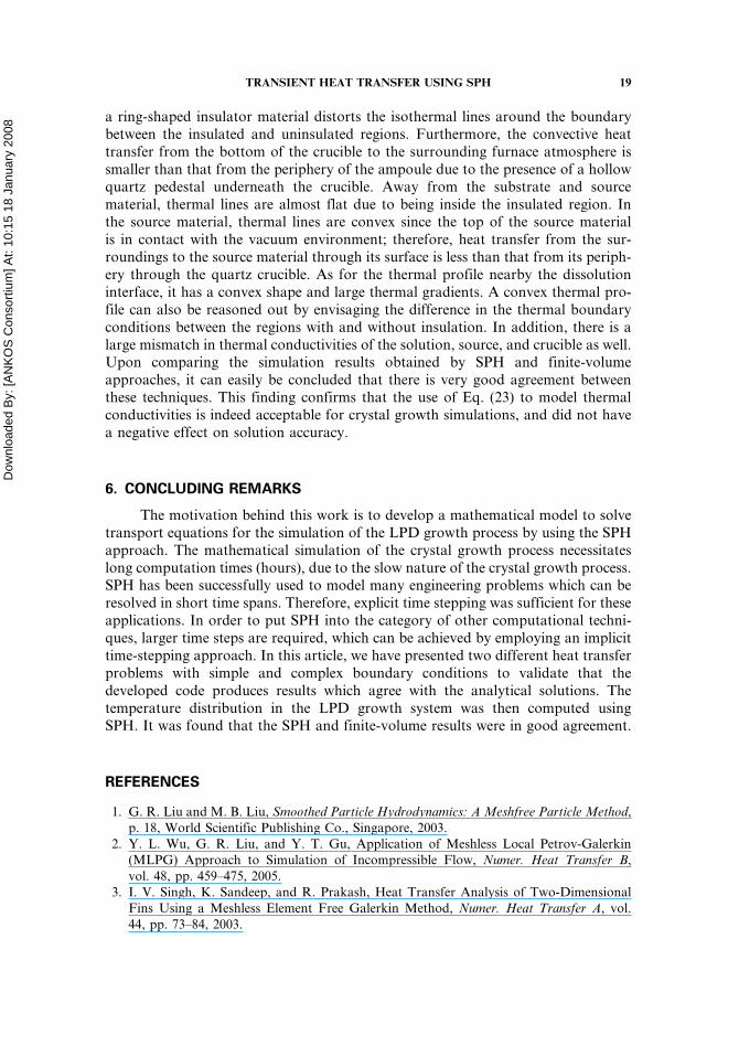
Figure 9. Simulation times versus number of SPH particles for explicit and Crank-Nicolson time

integration schemes.

14 R. ROOK ET AL.

Dow

nloa

ded

By:

[AN

KO

S C

onso

rtium

] At:

10:1

5 18

Jan

uary

200

8 in Figure 8. In addition to the above simulations, testing was carried out in order todetermine the computational time dependence on the number of SPH particles used.These tests incorporated simulations using both explicit and Crank-Nicolson timeintegration schemes for a simulation to t¼0:5 s. The result is given in Figure 9.

It was observed that the Crank-Nicolson implicit approach did not produce anobvious increase in solution accuracy compared with explicit time stepping. How-ever, the Crank-Nicolson time step was half of that required by the explicit techniquegiven by Eq. (12) to produce equivalent results. However, it was found that in theexplicit approach, if the time step was greater than that permitted by Eq. (12), thesolution broke down and did not converge. For these 2-D problems, the Crank-Nicolson solutions were unconditionally stable.

5. TRANSIENT CONDUCTION MODELING OF SEMICONDUCTORCRYSTAL GROWTH

A liquid-phase diffusion (LPD) Si0:05Ge0:95 crystal growth simulation has beencarried out, using a mesh-dependent finite-volume approach [23, 24]. However, incrystal growth simulations one must track the solid=liquid material interface asthe growth progresses, which is very cumbersome due to the mesh adaptationsrequired at each time step. Therefore, SPH is currently being investigated as an alter-native simulation approach to crystal growth modeling, as no mesh is required inSPH.

LPD is a solution growth technique within the family of directional solidifi-cation. In this technique, the solvent material (Ge) is located between a single-crystalsubstrate (Ge) and polycrystalline source material (Si). The charge materials are con-tained in a quartz crucible and are exposed to an axial temperature gradient. Initiallyall charge materials are solid. As the system is heated to the growth temperature, thesolvent Ge melts whereas the substrate melts partially and the silicon remains soliddue its higher melting temperature. The solvent starts dissolving source materialaccording to the binary SiGe phase diagram, hence producing the SiGe liquid phase.Silicon species are then transported toward the Ge substrate through diffusion andconvection. When the liquid mixture in the vicinity of the growth interface becomessupersaturated, solidification takes place due to constitutional supercooling, therebyproducing a single crystal. The silicon depletion in the solution is then replenished bythe dissolution of source material. A more detailed description of the LPD system isavailable in the literature [23].

In Figure 10, the computational geometry is presented along with the represen-tative thermal profile. A portion of the growth zone is covered by an annular insu-lator to allow a steep thermal profile in the vicinity of the growth interface. Here, theliquid phase represents a dilute binary mixture of silicon (solute) and germanium(solvent). The binary mixture is assumed to be a heat conducting incompressibleNewtonian fluid. The solid phases, Ge single-crystal substrate, silicon source, andthe quartz crucible, are considered to be heat-conducting rigid materials. The inter-face between the substrate and liquid is referred to as the growth interface, and theone between the liquid and source is the dissolution interface.

Figure 11 illustrates the two-dimensional SPH and finite-volume domains usedto discretize the LPD crystal growth system. All dimensions are given in meters.

TRANSIENT HEAT TRANSFER USING SPH 15

Dow

nloa

ded

By:

[AN

KO

S C

onso

rtium

] At:

10:1

5 18

Jan

uary

200

8

Here, the total number of particles used was N¼2;754; where the initial smoothinglength was taken as h¼0:5 mm. The quartz crucible is represented by � particles, particles represent the SiGe solution, and & and � particles represent the Ge sub-strate and Si source particles, respectively. As before, the symbol denotes particlesthat lie on the domain boundary.

For the finite-volume simulation, the respective mesh sizes for each materialregion are given in Table 1.

Figure 10. Computational domain of the LPD crystal growth system.

Figure 11. SPH and finite-volume domains for LPD simulation.

16 R. ROOK ET AL.

Dow

nloa

ded

By:

[AN

KO

S C

onso

rtium

] At:

10:1

5 18

Jan

uary

200

8

It has been shown [25] that the thermal profile may be computed independentlyof the flow field in liquid-phase diffusion crystal growth. That is, even though par-ticles will move during the simulation according to the solution of the Navier–Stokesequations, this convective flow will not have a significant effect on the temperaturefield. This assumption was deduced from a dimensional analysis, where the com-puted Prandtl number, a ratio between convective and conductive effects, was foundto be 0:0075 for the LPD system. As long as the Prandtl number is significantly lessthan one, the thermal transport across the solution is dominated by conduction, asopposed to the convective transport of fluid.

The thermal boundary conditions for the vertical wall, and the top and bottomsurfaces of the quartz crucible, are modeled with the equation

�jSqT

qn¼ H½T � Tf ðzÞ� ð20Þ

where Tf ðzÞ is the experimentally obtained ambient temperature inside the furnacealong the quartz ampoule wall or on the top and bottom surfaces, H is the modifiedheat transfer coefficient, including the contribution of convective and radiativeeffects on the heat transfer. The modified heat transfer coefficient was approximatedusing preliminary experimental results, such as the measured thermal profile, solutedistribution in a grown crystal, and the position of the initial growth interface [24].In addition, perfect thermal contact at the melt–ampoule, crystal–ampoule, andinner–outer crucible was assumed. At these boundaries, the heat flux was assumedto be continuous.

Table 2 lists the numerical values for the physical parameters used in the cur-rent model [25]. As well, since there are several materials present in the LPD system,the particle conductivity was modeled according to

ji !2jijj

ji þ jjð23Þ

derived by Monaghan and Cleary [19].

Table 1. LPD finite-volume simulation mesh sizes

Domain region Mesh size

Si source 10� 50

SiGe solution 80� 50

Ge substrate 30� 50

Quartz ampoule 1,200� 10

Table 2. Physical properties of the LPD system

Parameter Si source at T¼1; 300 K Ge substrate at T¼1; 210 K SiGe liquid Quartz

cp (J=kg K) 967 396.1 380–406 1,200

j (W=m K) 23.7 10.60 42.8 2.0

q (kg=m3) 2,301.6 5,323 5,633 2,200

TRANSIENT HEAT TRANSFER USING SPH 17

Dow

nloa

ded

By:

[AN

KO

S C

onso

rtium

] At:

10:1

5 18

Jan

uary

200

8 Use of the substitution equation (23) to model material regions having dissimi-lar thermal conductivities is a significant advantage of SPH over traditional finite-volume approaches. In the finite-volume simulations, the interface between twomaterials is required to have a boundary condition such that the heat flux is continu-ous. Computationally speaking, this approach is more expensive in terms of anadditional boundary treatment within the computational domain. Alternatively,use of the SPH conductivity eliminates the need for special material treatment withinthe computational domain, as well as greatly simplifies the implementation.

Figure 12 illustrates the SPH and finite-volume [25] solutions to the thermalprofile at t¼0:5 h, with all temperatures given in kelvin. As before, a Crank-Nicolson implicit time integration was used, allowing a time step of Dt¼0:5 s. Theblack lines represent material boundaries, with the concave lines indicating thecomputed growth interface.

Figure 12a shows the SPH computed temperature distributions in thesubstrate, solution, source, and quartz crucible for 0.5 h of growth time. As can beseen from Figure 12a, the initial growth interface deformed according to a referenceisothermal line (the melting temperature of germanium, T ¼ 1211:45 K) and is of aconcave shape. The formation of a concave interface could be attributed to severalreasons. The large mismatch in thermal conductivities of the substrate, solution, andsurrounding quartz crucible bends isothermal lines in the vicinity of the interface.Recalling the experimental configuration in Figure 10, there is an annular insulatormaterial located inside the furnace, which encompasses the quartz crucible with a3–5-mm clearance. The insulator material spans from approximately 5 mm abovethe substrate to the bottom of the source material. The convective heat transfer inthis semi-insulated region is handled by a proper estimate for the heat transfercoefficient, including both radiative and convective heat transfer. The presence of

Figure 12. SPH and finite-volume temperature field at t ¼ 0:5 h.

18 R. ROOK ET AL.

Dow

nloa

ded

By:

[AN

KO

S C

onso

rtium

] At:

10:1

5 18

Jan

uary

200

8 a ring-shaped insulator material distorts the isothermal lines around the boundarybetween the insulated and uninsulated regions. Furthermore, the convective heattransfer from the bottom of the crucible to the surrounding furnace atmosphere issmaller than that from the periphery of the ampoule due to the presence of a hollowquartz pedestal underneath the crucible. Away from the substrate and sourcematerial, thermal lines are almost flat due to being inside the insulated region. Inthe source material, thermal lines are convex since the top of the source materialis in contact with the vacuum environment; therefore, heat transfer from the sur-roundings to the source material through its surface is less than that from its periph-ery through the quartz crucible. As for the thermal profile nearby the dissolutioninterface, it has a convex shape and large thermal gradients. A convex thermal pro-file can also be reasoned out by envisaging the difference in the thermal boundaryconditions between the regions with and without insulation. In addition, there is alarge mismatch in thermal conductivities of the solution, source, and crucible as well.Upon comparing the simulation results obtained by SPH and finite-volumeapproaches, it can easily be concluded that there is very good agreement betweenthese techniques. This finding confirms that the use of Eq. (23) to model thermalconductivities is indeed acceptable for crystal growth simulations, and did not havea negative effect on solution accuracy.

6. CONCLUDING REMARKS

The motivation behind this work is to develop a mathematical model to solvetransport equations for the simulation of the LPD growth process by using the SPHapproach. The mathematical simulation of the crystal growth process necessitateslong computation times (hours), due to the slow nature of the crystal growth process.SPH has been successfully used to model many engineering problems which can beresolved in short time spans. Therefore, explicit time stepping was sufficient for theseapplications. In order to put SPH into the category of other computational techni-ques, larger time steps are required, which can be achieved by employing an implicittime-stepping approach. In this article, we have presented two different heat transferproblems with simple and complex boundary conditions to validate that thedeveloped code produces results which agree with the analytical solutions. Thetemperature distribution in the LPD growth system was then computed usingSPH. It was found that the SPH and finite-volume results were in good agreement.

REFERENCES

1. G. R. Liu and M. B. Liu, Smoothed Particle Hydrodynamics: A Meshfree Particle Method,p. 18, World Scientific Publishing Co., Singapore, 2003.

2. Y. L. Wu, G. R. Liu, and Y. T. Gu, Application of Meshless Local Petrov-Galerkin(MLPG) Approach to Simulation of Incompressible Flow, Numer. Heat Transfer B,vol. 48, pp. 459–475, 2005.

3. I. V. Singh, K. Sandeep, and R. Prakash, Heat Transfer Analysis of Two-DimensionalFins Using a Meshless Element Free Galerkin Method, Numer. Heat Transfer A, vol.44, pp. 73–84, 2003.

TRANSIENT HEAT TRANSFER USING SPH 19

Dow

nloa

ded

By:

[AN

KO

S C

onso

rtium

] At:

10:1

5 18

Jan

uary

200

8 4. I. V. Singh, Meshless EFG Method in Three-Dimensional Heat Transfer Problems:A Numerical Comparison, Cost and Error Analysis, Numer. Heat Transfer A, vol. 46,pp. 199–220, 2004.

5. I. V. Singh and P. K. Jain, Parallel Meshless EFG Solution for Fluid Flow Problems,Numer. Heat Transfer B, vol. 48, pp. 45–66, 2005.

6. J. Y. Tan, L. H. Liu, and B. X. Li, Least-Squares Collocation Meshless Approach forCoupled Radiative and Conductive Heat Transfer, Numer. Heat Transfer B, vol. 49,pp. 179–195, 2006.

7. T. Sophy, H. Sadat, and C. Prax, A Meshless Formulation for Three-Dimensional Lami-nar Natural Convection, Numer. Heat Transfer B, vol. 41, pp. 433–445, 2002.

8. L. B. Lucy, A Numerical Approach to the Testing of the Fission Hypothesis, Astro. J.,vol. 82, pp. 1013–1024, 1977.

9. R. A. Gingold and J. J. Monaghan, Smooth Particle Hydrodynamics: Theory andApplication to Non-Spherical Stars, Mon. Not. R. Astron. Soc., vol. 181, p. 375,1977.

10. L. D. G. Sigalotti, J. Klapp, E. Sira, Y. Mele�aan, and A. Hasmy, SPH Simulations of Time-Dependent Poiseuille Flow at Low Reynolds Numbers, J. Comput. Phys., vol. 191,pp. 622–638, 2003.

11. Y. Zhu and P. J. Fox, Smoothed Particle Hydrodynamics Model for Diffusion throughPorous Media, Transport Porous Media, vol. 43, pp. 441–471, 2001.

12. M. B. Liu, G. R. Liu, and K. Y. Lam, A One-Dimensional Meshfree Particle Formulationfor Simulating Shock Waves, Shock Waves, vol. 13, pp. 201–211, 2003.

13. A. Colagrossi and M. Landrini, Numerical Simulation of Interfacial Flows by SmoothedParticle Hydrodynamics, J. Comput. Phys., vol. 191, pp. 448–475, 2003.

14. P. Cleary, J. Ha, V. Alguine, and T. Nguyen, Flow Modelling in Casting Processes,Applied Mathematical Modelling, vol. 26, pp. 171–190, 2002.

15. S. Dost and Z. Qin, A Numerical Simulation Model for Liquid Phase ElectroepitaxialGrowth of GaInAs, J. Crystal Growth, vol. 187, pp. 51–64, 1998.

16. Y. C. Liu, Y. Okano, and S. Dost, The Effect of Applied Magnetic Field on Flow Struc-tures in Liquid Phase Electroepitaxy—A Three-Dimensional Simulation Model, J. CrystalGrowth, vol. 244, pp. 12–26, 2002.

17. S. Dost, Y. Liu, and B. Lent, A Numerical Simulation Study for the Effect of AppliedMagnetic Field in Liquid Phase Electroepitaxy, J. Crystal Growth, vol. 240, pp. 39–51,2002.

18. J. J. Monaghan, Implicit SPH Drag and Dusty Gas Dynamics, J. Comput. Phys., vol. 138,pp. 801–820, 1997.

19. P. W. Cleary and J. J. Monaghan, Conduction Modelling Using Smoothed ParticleHydrodynamics, J. Comput. Phys., vol. 148, pp. 235–236, 1999.

20. J. Bonet and M. X. Rodriguez-Paz, Hamiltonian Formulation of the Variable-h SPHEquations, J. Comput. Phys., vol. 209, pp. 541–558, 2005.

21. S. J. Cummins and M. Rudman, An SPH Projection Method, J. Comput. Phys., vol. 152,pp. 584–607, 1999.

22. M. N. Ozisik, Heat Conduction, 2nd ed., p. 75, Wiley, New York, 1993.23. M. Yildiz, S. Dost, and B. Lent, Growth of Bulk SiGe Single Crystals by Liquid Phase

Diffusion, J. Crystal Growth, vol. 280, pp. 151–160, 2005.24. M. Yildiz and S. Dost, A Continuum Model for the Liquid Phase Diffusion Growth of

Bulk SiGe Single Crystals, Int. J. Eng. Sci., vol. 43, pp. 1059–1080, 2005.25. M. Yildiz, A Combined Experimental and Modelling Study for the Growth of SixGe1�x

Single Crystals by Liquid Phase Diffusion (LPD), Ph.D. thesis, The University ofVictoria, Victoria, BC, Canada, 2005.

20 R. ROOK ET AL.

Dow

nloa

ded

By:

[AN

KO

S C

onso

rtium

] At:

10:1

5 18

Jan

uary

200

8 APPENDIX

In general, a scalar function f ðx1i ; x

2i ; ; x

ni Þ ¼ f ðxb

i Þ of the position vector xbi can

be represented by a Taylor series, expanded around the vector location xbj as

f ðxbi Þ ¼

X1k¼0

1

k!xc

ijðÞ;ch ik

f ðxbi Þ xb

i ¼xbj

" #ðA:1Þ

where the ðÞ;c operator denotes covariant differentiation with respect to coordinatexc

i . If we expand Eq. (A.1), we obtain, explicitly,

f ðxbi Þ ¼ f ðxb

j Þ þ xcijf;cðxb

j Þ þxc

ijxkij

2f;ckðxb

i Þ xb

i ¼xbj

þ � � � ðA:2Þ

since the difference vector xcij is a constant and can be pulled out of the covariant

derivative expression.To find the SPH approximation for the Laplacian operator, we begin by mul-

tiplying the Taylor series expansion of Eq. (A.2) with the term xaijW;aðxij; hÞ=gmnxm

ijxnij

producing

f ðxbi Þ � f ðxb

j Þh i

xaij

gmnxmijx

nij

W;aðxij ; hÞ ¼xc

ijxaij

gmnxmijx

nij

W;aðxij ; hÞf;cðxbj Þ

þxc

ijxkijx

aij

2gmnxmijx

nij

W;aðxij; hÞf;ckðxbi Þ xb

i¼xb

j

þ � � �

We then integrate over all three-dimensional space in dX ¼ dxbi coordinates, which

yields (after noting that the first integral term has an integrand with an odd function,and therefore goes to zero when integrated over all space)

ZZZX

f ðxbi Þ � f ðxb

j Þh i

xaij

gmnxmijx

nij

W;aðxij ; hÞdX ¼f;ckðxb

j Þ2

ZZZX

xcijx

kijx

aij

gmnxmijx

nij

W;aðxij; hÞdX

ðA:3Þ

up to second order. Expanding the integrand on the right-hand side using the pro-duct rule gives

xcijx

kijx

aij

gmnxmijx

nij

W;aðxij ; hÞ ¼xc

ijxkijx

aij

gmnxmijx

nij

Wðxij ; hÞ !

;a

�Wðxij ; hÞxc

ijxkijx

aij

gmnxmijx

nij

!;a

which produces

ZZZX

xcijx

kijx

aij

gmnxmijx

nij

W;aðxij ; hÞdX ¼ZZZ

X

xcijx

kijx

aij

gmnxmijx

nij

Wðxij ; hÞ !

;a

dX

�ZZZ

XWðxij ; hÞ

xcijx

kijx

aij

gmnxmijx

nij

!;a

dX

TRANSIENT HEAT TRANSFER USING SPH 21

Dow

nloa

ded

By:

[AN

KO

S C

onso

rtium

] At:

10:1

5 18

Jan

uary

200

8 for the integral on the right-hand side of Eq. (A.3). Using the divergence theorem forthe first integral on the right-hand side of the above equation gives

ZZZX

xcijx

kijx

aij

gmnxmijx

nij

W;aðxij ; hÞdX ¼ZZ

S

xcijx

kijx

aij

gmnxmijx

nij

Wðxij; hÞ !

nadS

�ZZZ

XWðxij; hÞ

xcijx

kijx

aij

gmnxmijx

nij

!;a

dX

Once again, we have the surface integral vanishing for all interior particlessince the kernel goes to zero, leaving

ZZZX

xcijx

kijx

aij

gmnxmijx

nij

W;aðxij ; hÞdX ¼ �ZZZ

X

Wðxij ; hÞxc

ijxkijx

aij

gmnxmijx

nij

!;a

dX ðA:4Þ

Expansion of the derivative in the integrand of Eq. (A.4) yields

xcijx

kijx

aij

gmnxmijx

nij

!;a

¼ 1

gmnxmijx

nij

xcijx

kijx

aij

� �;aþxc

ijxkijx

aij

1

gmnxmijx

nij

!;a

¼dc

axkijx

aij þ xc

ijdkaxa

ij þ xcijx

kijd

aa

gmnxmijx

nij

�xc

ijxkijx

aijgrw xr

ij;axwij þ xr

ij xwij;a

� �gmnxm

ijxnijggfx

gij x

fij

¼5xc

ijxkij

gmnxmijx

nij

�xc

ijxkijx

aijgawxw

ij þ xcijx

kijx

aijgraxr

ij

gmnxmijx

nijggfx

gij x

fij

¼3xc

ijxkij

gmnxmijx

nij

ðA:5Þ

Now, using Eq. (A.5) in Eq. (A.4) gives the result

ZZZX

xcijx

kijx

aij

gmnxmijx

nij

W;aðxij ; hÞdX ¼ �ZZZ

X

3xcijx

kij

gmnxmijx

nij

Wðxij; hÞdX ðA:6Þ

The second-order tensor in the above equation must be an isotropic tensor, since thekernel is a symmetric function multiplied by an even function. An isotropic tensor isone that can be written in terms of a constant c and the Kronecker delta as cdc

r.However, since the integral on the right-hand side of Eq. (A.6) has two contravariantfree indices c and k, we raise an index of our isotropic tensor with multiplication ofthe metric, so that

�ZZZ

X

3xcijx

kij

gmnxmijx

nij

Wðxij ; hÞdX ¼ cgkrdcr ðA:7Þ

22 R. ROOK ET AL.

Dow

nloa

ded

By:

[AN

KO

S C

onso

rtium

] At:

10:1

5 18

Jan

uary

200

8 is the appropriate representation of the isotropic tensor. The constant c can be foundfrom inner multiplication of the above equation with the metric gck, producing

�gck

ZZZX

3xcijx

kij

gmnxmijx

nij

Wðxij ; hÞdX ¼ cgckgkrdcr ¼ cdc

c ðA:8Þ

which, since the kernel is normalized, yields c ¼ �1. Substituting this value of c intoEq. (A.7), and using the results of Eqs. (A.6), and (A.3), we obtain, up to secondorder,

ZZZX

f ðxbi Þ � f ðxb

j Þh i

xaij

gmnxmijx

nij

W;aðxij; hÞdX ¼ � gckf;ckðxbi Þ

2

xb

i ¼xbj

which can be rewritten as

gckf;ckðxbj Þ

D E¼ 2

ZZZX

f ðxbj Þ � f ðxb

i Þh i

xaij

gmnxmijx

nij

W;aðxij; hÞdX

Our final result for the SPH Laplacian of a scalar field is written in terms ofparticle i by letting i! j and j ! i, noting that xb

ij ¼ �xbji and W;a ¼ �W;aj

, to yield

gckf;ckðxbi Þ

D E¼ 2

ZZZX

f ðxbi Þ � f ðxb

j Þh i

xaij

gmnxmijx

nij

W;aðxij; hÞdX ðA:9Þ

where all covariant derivatives in the above equation are with respect to xbi coordinates.

TRANSIENT HEAT TRANSFER USING SPH 23