Sigma Algebras in Probabilistic Epistemic Dynamics

Luca AcetoSchool of Computer Science

Reykjavík UniversityIS-101 Reykjavík, Iceland

luca@ru.is

Wiebe van der HoekDept. of Computer Science

University of LiverpoolLiverpool, UK

Wiebe.van-der-Hoek@liverpool.ac.uk

Anna IngolfsdottirSchool of Computer Science

Reykjavík UniversityIS-101 Reykjavík, Iceland

annai@ru.is

Joshua SackLong Beach, California

United Statesjoshua.sack@gmail.com

ABSTRACTThis paper extends probabilistic dynamic epistemic logicfrom a finite setting to an infinite setting, by introducingσ-algebras to the probability spaces in the models. Thismay extend the applicability of the logic to a real world set-ting with infinitely many possible measurements. It is shownthat the dynamics preserves desirable properties of measur-ability and that completeness of the proof system holds withthe extended semantics.

Categories and Subject DescriptorsF.4.1 [Mathematical Logic]: Modal Logic; F.4.1 [Mathe-matical Logic]: Proof Theory; I.2.4 [Artificial Intelli-gence]: Knowledge Representation Formalisms and Meth-ods

General TermsTheory

Keywordsdynamic epistemic logic, modal logic, probability

1. INTRODUCTIONA logic that combines probability, epistemics, and dynam-

ics provides us with a tool for describing how qualitativeand quantitative uncertainty change when given new infor-mation. A family of existing such logics [5, 8, 10], calledprobabilistic dynamic epistemic logics, stems from the paper[3] that introduced probabilistic epistemic logic, which canexpress interaction between qualitative and quantitative un-certainty. The setting of probabilistic epistemic logic in [3]

ACM COPYRIGHT NOTICE. Permission to make digital or hardcopies of all or part of this work for personal or classroom use isgranted without fee provided that copies are not made or distributedfor profit or commercial advantage and that copies bear this noticeand the full citation on the first page. To copy otherwise, to re-publish, to post on servers or to redistribute to lists, requires priorspecific permission and/or a fee. Request permissions from PublicationsDept., ACM, Inc., fax +1 (212) 869-0481, or permissions@acm.org.TARK 2011, July 12-14, 2011, Groningen, The Netherlands.Copyright c©2011 ACM. ISBN 978-1-4503-0707-9, $10.00.

involved probabilities over σ-algebras and potentially infi-nite sample spaces; however, the dynamic extensions in [5,10] are restricted to a finite setting. An infinite setting allowsus to model situations in which there may be measurementsover infinitely many possibilities, and in which there may be,for example, a normal or uniform distribution over a contin-uum of possibilities. The paper [8] explored semantics andproof systems that extend the probabilistic dynamic epis-temic logic in [5] to an infinite setting. Yet there remainedquestions, such as whether one can define the semantics insuch a way that the dynamics preserves the property thatthe denotation of a formula can be assigned a probability (itwas shown that such a property need not be preserved in thegeneral semantics given in [8]), and whether the complete-ness proof of [5] can be adapted to the infinite setting. Inthis paper, we answer these questions in the affirmative, butfor an extension of the richer and more recently developedlogic in [10], rather than for the extension of the logic in [5].

The logic in [10] involves three types of probabilities: prior,observation, and occurrence. Prior probabilities are subjec-tive probabilities that agents had before an event. Observa-tion probabilities are subjective probabilities that agents hadabout what event actually occurred. Occurrence probabili-ties are objective probabilities concerned with what eventactually occurs. The prior probabilities lie in the originalmodel, called a probabilistic epistemic model (the seman-tic structure in [3]), and the other two probabilities aregiven in another structure we call the update frame, which iscombined with the prior model to form a new probabilisticepistemic model with posterior probabilities. The work in[8] did include prior and observation probabilities, but didnot include occurrence probabilities, and this paper offers aframework that describes the interplay of all three types ofprobabilities in a setting in which the probabilities in theprobabilistic epistemic models (the prior probabilities) arepotentially infinite.

We present in the next section probabilistic epistemic logic,which will be the foundation for the dynamic extension thispaper will focus on. In addition, the semantic structures,probabilistic epistemic models, will be the structures com-prising the semantics that all the languages in this paper willbe interpreted over. These structures will involve probabili-ties defined on sigma algebras, and will be in an infinite set-

191

ting. Section 3 will introduce our version of dynamic prob-abilistic epistemic logic, by first introducing update framesand then by providing the semantics. It is shown in thissection (Theorem 1) that dynamics preserves the propertythat the denotation of every formula is measurable. Section4 will introduce a sound and complete proof system for thelogic with respect to the semantics given in Section 3.

2. PROBABILISTIC EPISTEMIC LOGICThe logic we will focus on, which we call Update Logic,

builds on Probabilistic Epistemic Logic, which we cover inthis section.

We first provide some definitions.

• A σ-algebra over a set S is a non-empty set of subsetsof S closed under countable unions and complements.

• Given a σ-algebra A, a function µ : A → [0,∞] iscalled a measure if µ(∪∞i=1Ai) =

P∞i=1 µ(Ai) for pair-

wise disjoint Ai ∈ A. This condition is called count-able additivity.

• A finite measure is a measure such that all of its valuesare finite.

• A measure space is a tuple (S,A, µ), where S is a set, Ais a σ-algebra over S, and µ : A → [0,∞] is a measure.

We focus throughout this paper on a variation of probabilityspaces that also includes the 0 function. Given a set X, letspaces(X) be the set of measure spaces (S,A, µ), such thatS ⊆ X and µ is a finite measure normalized to 0 or 1, thatis, µ(S) is either 0 or 1. The structures over which we willinterpret formulas have Kripke frames as a core component.

Definition 1. [Kripke frame] Given a set I, which we willassociate with a group of agents, a Kripke frame for I is atuple F = (X,R), where

• X is a set of states called the carrier set of F , and

• R : I→ X×X is a function assigning a binary relationR` to each agent in ` ∈ I.

We often write the superscript F for each component toemphasize which structure the components are in. Thatis, we might write XF for X and RF for R. Since we arein a multi-agent setting, we call the relations R` epistemicrelations, and view xR`y to mean that ` considers y possiblegiven x. But while epistemic relations are generally viewedas equivalence relations, we for simplicity do not impose anyrestrictions on them.

When we add to a Kripke frame a component that dec-orates each state with properties called atomic propositionsand another component that decorates states with measurespaces, we obtain the type of structure over which we willinterpret our formulas. We call these structures probabilisticepistemic models.

Definition 2. [Probabilistic Epistemic Model] Given a setAtProp of atomic propositions and a set I of agents, we definea probabilistic epistemic model for AtProp and I as a tupleM = (X,R, V,P), where

• (X,R) is a Kripke frame for I,• V : AtProp→ P(X) is a “valuation” function, and

• P : I ×X → spaces(X) is a function associating everyagent ` and element x with a measure space P`,x =(S`,x,A`,x, µ`,x), where S`,x ⊆ X.

A pair (M,x) with x ∈ X is called a pointed model.

The measure space P`,x represents agent `’s subjective viewof the likelihoods of certain subsets of the model if the actualstate were x. We generally omit the superscripts M whenthey are understood from context. Similarly we may omitexplicit mention of AtProp and I when they are understoodfrom context. We may also omit the σ-algebra componentof the measure space P`,x, when that component is just thesame as the power set of the sample space. A Kripke frameor a probabilistic epistemic model is said to be finite if itscarrier set is finite.

2.1 Probabilistic Epistemic Language

Definition 3. [Language LPEL] Given a set I of agents anda set AtProp of atomic propositions, the languageLPEL(I,AtProp) is given by the following Backus-Naur form:

ϕ ::= true | false | p | ¬ϕ | ϕ ? ϕ | [`]ϕ | t` ≥ qwhere p ∈ AtProp, ` ∈ I, q ∈ Q, and ? ∈ {∧,∨,→,↔}; foreach agent ` ∈ I,

t` ::= qP`(ϕ) | t` + t`

where q ∈ Q. We simply write LPEL for LPEL(I,AtProp)when I and AtProp are clear from the context or are imma-terial.

The formula false is not true anywhere, while true is trueeverywhere. The operators ¬, ∧, ∨, →, and ↔ have theirusual boolean readings of not, and, or, only if, and if andonly if respectively. The formula [`]ϕ is read as agent `believes ϕ. The formula q1P`(ϕ1) + · · · + qnP`(ϕn) ≥ qstates that a linear combination of probabilities for a specificagent is at least q. We use linear combinations for technicalreasons. In the linear combination, P`(ϕi) stands for theprobability that agent ` assigns to the truth of formula ϕi.We involve addition of probability terms, since additivity isa fundamental condition on measures and hence on prob-abilities. We restrict the probability terms of a particularprobability formula to ones that involve a single agent forsimplicity. The formulas inside the arguments of the proba-bility terms may involve other probability formulas for otheragents.

Abbreviations:.We have the usual modal abbreviation: 〈`〉ϕ def

= ¬[`]¬ϕ(read as agent ` considers ϕ possible). Also, if c ∈ Q andt =

Pnk=1 qkP`(ϕk) = q1P`(ϕ1) + · · · + qnP`(ϕn), we have

the following abbreviations.

ctdef=Pnk=1 cqkP`(ϕk)

t ≤ q def= −t ≥ −q

t < qdef= ¬(t ≥ q)

t > qdef= ¬(t ≤ q)

t = qdef= t ≤ q ∧ t ≥ q

t ≥ s def= t− s ≥ 0

t = sdef= t− s ≥ 0 ∧ s− t ≥ 0

192

SemanticsWe will define [[·]]LPEL as a function mapping LPEL to func-tions that map probabilistic epistemic models to subsets oftheir carrier set. We write [[ϕ]]M for [[ϕ]](M), and the setdenoted [[ϕ]]M is considered to consist of all states in M atwhich ϕ is true. Our probability formulas will involve ap-plying measures µM`,x to sets of the form [[ϕ]]M , as long as

[[ϕ]]M ∩SM`,x ∈ AM`,x. Two options for addressing the require-

ment that [[ϕ]]M∩SM`,x ∈ AM`,x are as follows. One is to place a

restriction on the models such that [[ϕ]]M ∩SM`,x ∈ AM`,x holdsfor every ϕ, ` and x. Another is to involve a commonly usedextension of the notion of a measure, called the outer mea-sure, which extends the domain of the measure to the wholepower set of the sample space (rather than just the sets inthe σ-algebra). Given a measure µ : A → [0,∞), the outermeasure extension of µ is defined to be µ∗ : P(S)→ [0,∞),given by

µ∗(A) = inf{µ(B) | B ∈ A, A ⊆ B}. (1)

The outer measure extension is indeed an extension [4]:µ(A) = µ∗(A) for each A ∈ A. We define the semanticsin the more general setting using the outer measure, andsince the outer measure extends the measure, the semanticsbehaves the same way on the restricted input model if wereplace the outer measure with the original measure.

We define [[·]]LPEL using the following rules:

[[ true]]MLPEL= XM

[[p]]MLPEL= VM (p)

[[¬ϕ]]MLPEL= XM − [[ϕ]]MLPEL

[[ϕ ∧ ψ]]MLPEL= semϕMLPEL

∩ [[ψ]]MLPEL

[[ϕ ∨ ψ]]MLPEL= [[ϕ]]MLPEL

∪ [[ψ]]MLPEL

[[ϕ→ ψ]]MLPEL= [[¬ϕ]]MLPEL

∪ [[ψ]]MLPEL

[[ϕ↔ ψ]]MLPEL= ([[ϕ]]MLPEL

∩ [[ψ]]MLPEL)

∪([[¬ϕ]]MLPEL∩ [[¬ψ]]MLPEL

)

[[[`]ϕ]]MLPEL= {x | RM` (x) ⊆ [[ϕ]]MLPEL

}[[q1P`(ϕ1) + · · ·+ qnP`(ϕn) ≥ q]]MLPEL

= {x |Pnk=1 qk(µM`,x

∗)([[ϕk]]MLPEL

∩ S`,x) ≥ q}We often omit the subscript LPEL and/or the superscript Mif they should be understood from context.

2.2 Comparing probability and epistemicsIt might seem natural to define belief by agent ` in the

truth of a formula as that formula having probability 1 foragent `. This might be difficult to enforce when the proba-bility measure is, for example, the uniform measure on theunit interval. For the uniform measure on the unit interval,what would be the set of related states? Surely it shouldhave probability 1, but given any set A of probability 1, onecan remove countably many states and still have a set A′

with probability 1. If we make the set of possibilities to bethe set A, then a formula true and only true on A′ wouldhave probability 1, but would not be believed. But the sit-uation improves if the probability measure has a countableσ-algebra and if the set of states at which a formula is trueis in the σ-algebra. Then we could define the set of relatedstates to be those states not contained in a set of measure 0.Note that this set cannot be empty, since if every elementwere contained in a set of measure 0, then the subadditivitycondition of measures would ensure that the sample space

also have measure 0, which would contradict the fact we areare assuming the measure is normalized to 1. By defining theset of related states to be those states not contained in anyset of measure 0, we obtain the following two relationships:

• 〈`〉ϕ↔ P`(ϕ) > 0 and

• [`]ϕ↔ P`(ϕ) = 1.

As pointed out in [3], however, it might be helpful to usethe flexibility of the two components, and not to imposethe restriction that information believed is identified withinformation given probability 1. The example presented inthe above-cited reference involves an event, namely a bit be-ing output by a computer, and asserts that that this eventshould not be assigned a probability, since too little is knownabout how the computer determines what bit to output. Inaddition, the example considers the flipping of a fair coin,where the odds are known to be even for heads and tails.Although the probability of the bit is unknown, it can bedetermined that the probability of the combination of thebit being 1 and the coin flip resulting in heads is 0.5. Inorder to have a model that assigns this combination a prob-ability but to still reflect uncertainty about the coin flip, theexample considers a model in which the agent is epistemi-cally uncertain about two probability spaces: one space hasas its sample space outcomes where the bit is always 1, andthe other space has as its sample space outcomes where thebit is always 0. Thus probabilistic epistemic logic allows usto model agents who are subjectively uncertain about prob-ability spaces.

3. UPDATE LOGICIn this section, we adapt the probabilistic dynamic epis-

temic logic from [10] to an infinite setting. Probabilistic dy-namic epistemic logic adds to probabilistic epistemic logicoperators of the form [U, e]ϕ, where (U, e) is a structurecalled a pointed update frame. A pointed update frame rep-resents a communication that transforms one probabilisticepistemic model into another. We use essentially the sameupdate frames as in [10]; where we differ is that we, unlikein [10], will use the probabilistic epistemic models of theprevious section, that use σ-algebras.

Definition 4. [L-update frame] Given a set I of agents anda language L that extends propositional logic1, an L-updateframe for I is a tuple U = (X,R,Φ,P) such that

• (X,R) is a finite Kripke frame,

• Φ is a finite2 set of pairwise inconsistent3 formulascalled preconditions,

• P : (I × X) ∪ Φ → spaces(X) is a function associ-ating every agent ` and element e with a probabil-ity measure space P`,e = (X, P(X), µ`,e) and everyprecondition ϕ ∈ Φ with a probability measure spacePϕ = (X, P(X), µϕ).

1We really intend for the language to extend LPEL, but weemphasize propositional logic, since we will make use of dis-junctions of L formulas in forming notation used throughoutthis section.2The restriction that this set be finite is closely related tothe fact that we are working with finitary languages.3Pairwise inconsistent formulas guarantee that their deno-tations be pairwise disjoint.

193

A pair (U, e) with e ∈ X is called a pointed update frame,with e being called the point of the pair (U, e).

We often write µϕ(e) for µϕ({e}), and similarly for othermeasures defined on singletons. The probabilities P`,e arecalled observation probabilities, and Pϕ are called occur-rence probabilities. Occurrence probabilities represent thelikelihood of the event actually happening. An example isgiven in [10], where a person wants to determine whether hehas a disease by observing a likely symptom of the disease,the symptom being the swelling of a gland. We considertwo preconditions: having the disease and not having thedisease. Hence we have two occurrence probability distribu-tions. One would assume the precondition that the personhas the disease and would give the likelihood that he has thesymptom, most likely large but with a probability less than1. The other would assume the precondition that he doesnot have the disease and would give the likelihood that hehas the symptom, most likely small, but with a probabilitygreater than 0.

We define a function pre : X → L, given by pre(e) =W{ϕ | µϕ(e) > 0}, where the empty disjunction is the for-mula false, which is not satisfied by any state in any model.Again, we often add superscripts of U to clarify which struc-ture components are in.

In what follows, when given a probabilistic epistemic modelM , for each s ∈ Sϕ∈Φ[[ϕ]]M , let ϕ(s) be the precondition

ϕ ∈ Φ for which s ∈ [[ϕ]]M . Also, for each set A ⊆ XM×XU ,let Ae = {(x, f) ∈ A | f = e}, and let πj be the projectionfunction taking an tuple and returning its jth component.

Definition 5. [Update product] The update product be-tween a probabilistic epistemic model M and an L-updateframe U is the probabilistic epistemic model M [U ] with thefirst three components:

• XM [U ] = {(x, e) | x ∈ [[ pre(e)]]M},• (x, e)R

M [U ]` (y, f) iff xRM` y and eRU` f ,

• ‖p‖M [U ] = {(x, e) ∈ XM [U ] | x ∈ ‖p‖M},and the last component

PM [U ]

`,(x,e) = (SM [U ]

`,(x,e),AM [U ]

`,(x,e), µM [U ]

`,(x,e))

defined by:

• SM [U ]

`,(x,e) = {(y, e) ∈ XM [U ] | y ∈ SM`,x},• AM [U ]

`,(x,e) is the smallest σ-algebra containing

{A×B | A ∈ AM`,x, B ∈ P(XU )} ∩ P((XM [U ])2),

• and

µM [U ]

`,(x,e)(C) = N/D, (2)

where

N =Xϕ∈Φ

Xf∈XU

µUϕ ({f}) · µU`,e({f})·

µM`,x([[ϕ ∧ pre(f)]]M ∩ SM`,x ∩ π1(C))

and

D =Xϕ∈Φ

Xf∈XU

µUϕ ({f}) · µU`,e({f})·

µM`,x([[ϕ ∧ pre(f)]]M ∩ SM`,x),

if the denominator D is not 0; otherwise µM [U ]

`,(x,e) = 0,

the zero measure.

The function µM [U ]

`,(x,e) is a measure, since it is a finite lin-

ear combination of measures µ`,x restricted to the domainsof the form [[ϕ ∧ pre(f)]]M ∩ S`,x. The denominator is thesame as the numerator except that it is given the largest in-put under this domain restriction, and hence represents thelargest value the numerator can obtain. If the denomina-tor is non-zero, this normalizes the quotient to a probabilitymeasure.

3.1 Update LanguageThe following definition is adapted from [6, 7].

Definition 6. [Language LUL] Given a set I of agents anda set AtProp of atomic propositions, the languageLUL(I,AtProp) is given by adding to the Bachus-Naur formof LPEL the formula [U, e]ϕ, where (U, e) is an LUL-updateframe.

Note that there are two sources of mutual recursion in thisdefinition. One, which is inherited from probabilistic epis-temic logic, is between terms and formulas. The other,which is inherited from dynamic epistemic logic (which hasnot been defined in this paper), is between formulas and up-date frames. The Bachus-Naur form generates the smallestsets of formulas, terms, and pointed update frames for whichthis mutual recursion holds.

The semantics of LUL is obtained by adding to the seman-tics of LPEL the following rule:

[[[U, e]ϕ]]M = [[¬ pre(e)]]M ∪ {x | (x, e) ∈ [[ϕ]]M [U ]}.Note that [[¬ pre(e)]]M∪{x | (x, e) ∈ [[ϕ]]M [U ]} = [[¬ pre(e)]]M∪π1([[ϕ]]

M [U ]e ). We may often write [[ϕ]] for [[ϕ]]M , when the

model M is clear from context.

3.2 Preserving measurability through updat-ing

Here we show that the dynamics of the semantics preservesthe property that a formula always denotes a measurable set.To be more precise, let mea be a function from probabilisticepistemic models M to P(P(XM )), such that

mea(M) = {Z ⊆ XM | Z ∩ SM`,x ∈ AM`,x ∀x ∈ XM , ` ∈ I}.Note that mea(M) is a σ-algebra.

Theorem 1. Suppose M is such that for every formulaϕ ∈ LUL, [[ϕ]]M ∈ mea(M). Then for any update frame U

and formula ϕ, we have that [[ϕ]]M [U ] ∈ mea(M [U ]).

Proof. Suppose M is such that for every formula ϕ ∈LUL, [[ϕ]]M ∈ mea(M). Fix an update frame U . Given aformula ϕ, we have that

[[ϕ]]M [U ] =[

e∈XU

[[ϕ]]M [U ]e . (3)

Now for each e, we have that

[[[U, e]ϕ]]Mdef= [[¬ pre(e)]]M ∪ π1([[ϕ]]M [U ]

e ) ∈ mea(M).

Thus, as [[¬ pre(e)]]M ∩ π1([[ϕ]]M [U ]e ) = ∅ and [[¬ pre(e)]]M ∈

mea(M),

π1([[ϕ]]M [U ]e ) ∈ mea(M).

194

Then using the definition of each AM [U ]

`,(x,e),

π1([[ϕ]]M [U ]e )× {e} ∈ mea(M [U ]).

As π1([[ϕ]]M [U ]e ) × {e} = [[ϕ]]

M [U ]e we have that [[ϕ]]

M [U ]e ∈

mea(M [U ]). As mea(M [U ]) is a σ-algebra, and in particular

is closed under finite unions, we have by (3) that [[ϕ]]M [U ] ∈mea(M [U ]).

4. PROOF SYSTEMWe now present a proof system for the validity of LUL.

The proof system, adapted from [8, 10], is given in Figure1. The schemes CL through UK, as well as the rules MP,[`]-NEC, and [U, s]-NEC are standard in dynamic epistemiclogic. The axiom UP describes the updating of a probabilityformula, and asserts that the update is equivalent to twodisjuncts. The first disjunct asserts that if the probabilityof the denominator of (2) is 0, then the updated measureis the 0 function. The second disjunct asserts that if thedenominator of (2) is positive, then the updated measure isgiven by (2). The axiom UP is essentially the same as thatin [10], except it accounts for the differences in the updatesemantics that allow for σ-algebras to be involved in theinput model. The schemes IP through P3 come from [3],with the exception of P2, which addresses the possibilitiesof our measures being the 0 measure. This was suggested in[8], but completeness was not addressed in that reference.Finally the rule EQV comes from [5, 8], and plays the samerole as the distributivity scheme in [3].

Theorem 2. The proof system given in Figure 1 is soundfor validity of LUL.

Proof. We limit ourselves to presenting the proofs foraxioms P2 and UP, which we consider in turn below.

Axiom P2.We prove the soundness of this axiom for an arbitrary

probabilistic epistemic model M . To this end, we reason asfollows:

= [[P`( true) = 1 ∨ P`( true) = 0]]M

= [[P`( true) = 1]]M ∪ [[P`( true) = 0]]M

= {x | (µM`,x)∗([[ true]]M ∩ S`,x) = 1}= ∪{x | (µM`,x)∗([[ true]]M ∩ S`,x) = 0}= {x | (µM`,x)∗(S`,x) = 1} ∪ {x | (µM`,x)∗(S`,x) = 0}= {x | µM`,x(S`,x) = 1} ∪ {x | µM`,x(S`,x) = 0}= {x | µM`,x(S`,x) = 1 or µM`,x(S`,x) = 0}= XM .

Axiom UP.Let U be an L-update frame for I. We limit ourselves to

proving that UP is valid over M when n = 1. The generalcase is only notationally more complex.

As in the statement of axiom UP, let

t =X

ϕ∈Φ,f∈XU

µϕ(f)µ`,e(f)P`(ϕ ∧ pre(f))

We wish to show that the denotation on the left-hand side ofthe implication is the same as the denotation on the right-hand side of the implication. Let (M,x) be an arbitrarypointed model, and consider two cases depending on whetherx ∈ [[t = 0]].

Axiom Schemes

CL. Schemes for Classical Propositional Logic

KK [`](ϕ→ ψ)→ ([`]ϕ→ [`]ψ)

KU [U, e](ϕ→ ψ)→ ([U, e]ϕ→ [U, e]ψ)

UA [U, e]p↔ ( pre(e)→ p) (p an atomic formula)

UC [U, e](ϕ ∧ ψ)↔ [U, e]ϕ ∧ [U, e]ψ

UN [U, e]¬ϕ↔ ( pre(e)→ ¬[U, e]ϕ)

UK [U, e][`]ϕ↔ ( pre(e)→ Vf :eR`f

[`][U, f ]ϕ)

UP [U, e](Pnk=1 qkP`(ψk) ≥ q)↔

t = 0 ∧ ( pre(e)→Pnk=1 qkP`( false) ≥ q))∨

¬(t = 0)∧( pre(e)→Pn

k=1 qkPϕ∈Φ,f∈XU µϕ(f)µ`,e(f)

P`(ϕ ∧ pre(f) ∧ [U, f ]ψk) ≥ qt)),where

t =Pϕ∈Φ,f∈XU µϕ(f)µ`,e(f)P`(ϕ ∧ pre(f))

IPPnk=1 qkP`(ϕk) ≥ q →Pn

k=1 qjkP`(ϕjk ) ≥ qfor permutation j1, . . . , jn of 1, . . . , n

I0 t ≥ q ↔ t+ 0P`(ϕk+1) ≥ qIA

Pnk=1 qkP`(ϕk) ≥ q ∧Pn

k=1 q′kP (ϕk) ≥ q′ →Pn

k=1(qk + q′k)P`(ϕk) ≥ (q + q′)

IM t ≥ q ↔ dt ≥ dq where d > 0

DICH (t ≥ q) ∨ (t ≤ q)MON (t ≥ q)→ (t > q′) where q > q′

P1 P`(ϕ) ≥ 0

P2 P`( true) = 1 ∨ P`( true) = 0

P3 P`(ϕ ∧ ψ) + P`(ϕ ∧ ¬ψ) = P`(ϕ)

Rules

` ϕ→ ψ ` ϕ` ψ (MP)

` ϕ` [`]ϕ

([`]-NEC)

` ϕ` [U, e]ϕ

([U, e]-NEC)

` ϕ↔ ψ

` P`(ϕ) = P`(ψ)(EQV)

Figure 1: The Proof System

195

Case x ∈ [[t = 0]]..We claim that

[[(t = 0) ∧ [U, e](q1P`(ψk) ≥ q)]]M

= [[(t = 0) ∧ ( pre(e)→ q1P`( false) ≥ q)]]M .If x 6∈ pre(e), then the right conjunct of each side of theequation is vacuously true, and hence the equation holds.Let us assume that x ∈ pre(e). First note that x ∈ [[t = 0]]M

if and only ifXϕ∈Φ

Xf∈XU

µUϕ ({f})µU`,e({f})

µM`,x([[ϕ ∧ pre(f)]]M ∩ SM`,x) = 0.

This is immediate from the fact that the set [[t = 0]]M isequal to

{x |X

(ϕ,f)∈Φ×XU

µUϕ ({f})µU`,e({f})

(µM`,x)∗([[ϕ]]M ∩ [[ pre(f)]]M ∩ SM`,x) = 0}.

Then by Definition 5, µM [U ]

`,(x,e) is the zero measure. Thus

under the assumption that x ∈ [[ pre(e)]]M , x ∈ [[(t = 0) ∧[U, e](q1P`(ψk) ≥ q)]]M if and only if q ≤ 0. For the righthand side, it is easy to see that under the assumption thatx ∈ [[ pre(e)]]M , x ∈ [[(t = 0) ∧ ( pre(e)→ q1P`( false) ≥ q)]]M

if and only if q ≤ 0, since µ`,x([[ false]]) = µ`,x(∅) = 0.

Case x 6∈ [[t = 0]]..We claim that

[[¬(t = 0) ∧ [U, e](q1P`(ψk) ≥ q)]]M =

[[¬(t = 0) ∧ ( pre(e)→q1Xϕ∈Φ

Xf∈XU

µϕ(f)µ`,e(f)

P`(ϕ ∧ pre(f) ∧ [U, f ]ψk) ≥ qt))]]M .Like in the case where x ∈ [[t = 0]]M , if x 6∈ [[ pre(e)]]M , thisequality is immediate. So assume that x ∈ [[ pre(e)]]M as wellas x 6∈ [[t = 0]]. Then we aim to show that for such x, thefollowing are equivalent:

1. x ∈ [[[U, e](q1P`(ψk) ≥ q)]]M

2. x ∈ [[q1Pϕ∈Φ

Pf∈XU µϕ(f) µ`,e(f) P`(ϕ ∧ pre(f) ∧

[U, f ]ψk) ≥ qt))]]M

First note that x ∈ [[[U, e](q1P`(ψk) ≥ q)]]M is equivalent to

x ∈ π1([[q1P`(ψ) ≥ q]]M [U ]e ). (4)

and by Definition 5, this is equivalent to q1N/D ≥ q, where

N =Xϕ∈Φ

Xf∈XU

µUϕ ({f})µU`,e({f})

µM`,x([[ϕ ∧ pre(f)]]M ∩ SM`,x ∩ π1([[ψ]]M [U ]))

and

D =Xϕ∈Φ

Xf∈XU

µUϕ ({f})µU`,e({f})

µM`,x([[ϕ ∧ pre(f)]]M ∩ SM`,x).

Multiplying both sides by the denominator, and then sub-tracting from both sides the new right hand side (all stepswhich are reversible), we obtain0BB@

q1Pϕ∈Φ

Pf∈XU µ

Uϕ ({f})µU`,e({f})

µM`,x([[ϕ ∧ pre(f)]]M ∩ SM`,x ∩ π1([[ψ]]M [U ]))−qPϕ∈Φ

Pf∈XU µ

Uϕ ({f})µU`,e({f})

µM`,x([[ϕ ∧ pre(f)]]M ∩ SM`,x)

1CCA ≥ 0 .

Then as π1([[ψ]]M [U ]) =Sf∈XU [[ pre(f)∧ [U, f ]ψ]]M , we have

that x is in266426640BB@

q1Pϕ∈Φ

Pf∈XU µ

Uϕ ({f})µU`,e({f})

P`(ϕ ∧ pre(f) ∧ [U, f ]ψ))−qPϕ∈Φ

Pf∈XU µ

Uϕ ({f})µU`,e({f})

P`(ϕ ∧ pre(f))

1CCA ≥ 0

37753775M

.

By adding qt to both sides we see that this is equivalent tox being in»»„

q1Pϕ∈Φ

Pf∈XU µϕ(f)µ`,e(f)

P`(ϕ ∧ pre(f) ∧ [U, f ]ψk)

«≥ qt

––M,

which completes the proof of the soundness of this case.

Other axioms and rules.The soundness of the remaining rules is standard following

the lead of [8, 10].

Theorem 3. The inference system given in Figure 1 isweakly complete for validity of LUL.

To prove completeness, we reduce the problem of complete-ness of the proof system for LUL with respect to the seman-tics in Section 3 to the better known completeness problemof probabilistic epistemic logic LPEL in [3]. We thus trans-late LUL into LPEL in such a way that every ϕ ∈ LUL istranslated into a t(ϕ) ∈ LPEL, such that ` ϕ↔ t(ϕ).

To help with induction on formulas, we impose an order onformulas using the following complexity function, adaptedfrom [2, 9, 7].

Definition 7. [Complexity] We define a complexity func-tion c : LUL → Z+ from formulas to positive integers asfollows:

c(a)def= 1 for a ∈ AtProp ∪ { false, true}

c(ϕ ? ψ)def= 1 + max{c(ϕ), c(ψ)} for ? ∈ {∧,∨,→,↔}

c(¬ϕ)def= 1 + c(ϕ)

c([`]ϕ)def= 1 + c(ϕ)

c([U, e]ψ)def= (2 + |XU |+ max{c( pre(f)) | f ∈ XU})

·2c(ψ)

c(Pnk=1 akP`(ϕk) ≥ b) def

= max{c(ϕk) + 1 | 1 ≤ k ≤ n}

Theorem 4. The function c from Definition 7 satisfieseach of the following.

1. If ψ is a proper subformula of ϕ, then c(ψ) < c(ϕ).

2. c( pre(e)→ q) < c([U, e]q) for q ∈ AtProp∪{ true, false}.

3. c([U, e]ϕ ? [U, e]ψ) < c([U, e](ϕ ? ψ)) for ? ∈ {∧,∨,→,↔}.

4. c( pre(e)→ ¬[U, e]ϕ) < c([U, e]¬ϕ).

196

5. c( pre(e)→ Vf :eRU

`f [`][U, f ]ϕ) < c([U, e][`]ϕ) for ` ∈ I.

6. c`(t = 0∧ ( pre(e)→Pn

k=1 qkP`( false) ≥ q)))∨ (¬(t =0)∧ ( pre(e)→Pn

k=1 qkPϕ∈Φ,f∈E µϕ(f)µe,`(f)P`(ϕ∧

pre(f) ∧ [U, f ]ψk) ≥ qt))´ < c([U, e]Pnk=1 qkP`(ψk)),

where t =Pϕ∈Φ,f∈E µϕ(f)µe,`(f)P`(ϕ ∧ pre(f)).

7. If c(ϕ) < c(ψ), then c([U, e]ϕ) < c([U, e]ψ).

Proof. This proof follows standard techniques, and wewill only provide a proof of the most surprising item, namelyitem 6:

c`(t = 0 ∧ ( pre(e)→Pn

k=1 qkP`( false) ≥ q))) ∨ (¬(t =0) ∧ ( pre(e)→Pn

k=1 qkPϕ∈Φ,f∈E µϕ(f)µe,`(f)P`(ϕ ∧

pre(f) ∧ [U, f ]ψk) ≥ qt))´ < c([U, e]Pnk=1 qkP`(ψk)), where

t =Pϕ∈Φ,f∈E µϕ(f)µe,`(f)P`(ϕ ∧ pre(f)).

Proceeding, we have the following argument:

c`(t = 0 ∧ ( pre(e)→

nXk=1

qkP`( false) ≥ q))) ∨

(¬(t = 0) ∧ ( pre(e)→nXk=1

Xϕ∈Φ,f∈E

qkµϕ(f)µe,`(f)

P`(ϕ ∧ pre(f) ∧ [U, f ]ψk)− qt ≥ 0))´

= 2 + max{c(t = 0),

c( pre(e)→nXk=1

qkP`( false) ≥ q),

c(¬t = 0),

c( pre(e)→nXk=1

Xϕ∈Φ,f∈E

qkµϕ(f)µe,`(f)

(P`(ϕ ∧ pre(f) ∧ [U, f ]ψk)

−qP`(ϕ ∧ pre(f)) ≥ 0)}= 4 + max

k,ϕ,f{c(ϕ ∧

pre(f) ∧ [U, f ]ψk), c(ϕ ∧ pre(f))}= 6 + max

k,f{c([U, f ]ψk)}

= 6 + |XU |+ maxk,f{(2 + c( pre(f))) · 2c(ψk)}

< (2 + |XU |+ maxf

c( pre(f)))

·(2 maxk{c(ψk)}+ 2)

= (2 + |XU |+ max c( pre(f)))

·2c(nXk=1

qkP`(ψk) ≥ q)

= c([U, e]nXk=1

qkP`(ψk) ≥ q)

There are different values for the complexity of an updateformula [U, s]ψ used in the literature. The one given in [9]sets c([U, e]ψ) = (4 + maxf c( pre(f)))c(ψ). We add a multi-plicity of 2 in order to handle the probabilistic update casein Theorem 4. But this also allows us to reduce the 4 to a 2in all the cases, even the non-probabilistic ones.

The following translation function is adapted from [7]:

t(q) = q for q ∈ Φ ∪ { true, false}t(¬ϕ) = ¬t(ϕ)t(ϕ1 ? ϕ2) = t(ϕ1) ? t(ϕ2) for ? ∈ {∧,∨,→,↔}t([`]ϕ) = [`]t(ϕ)t(Pnk=1 qkP`(ϕk) ≥ q) =

Pnk=1 qkP`(t(ϕk)) ≥ q

t([U, e]q) = t( pre(e)→ q) for q ∈ Φ ∪ { true, false}t([U, e]¬ϕ) = t( pre(e)→ ¬[U, e]ϕ)t([U, e](ϕ1 ? ϕ2)) = t([U, e]ϕ1 ? [U, e]ϕ2)

for ? ∈ {∧,∨,→,↔}t([U, e][`]ϕ) = t( pre(e)→ V

f :eR`f[`][U, f ]ϕ)

t([U, e]Pnk=1 qkP`(ϕk) ≥ q) =

t(τ = 0 ∧ ( pre(e)→Pnk=1 qkP`( false) ≥ q))∨

¬(τ = 0) ∧ ( pre(e)→Pnk=1 qk

Pϕ∈Φ,f∈E

µϕ(f)µe,`(f)P`(ϕ ∧ pre(f) ∧ [U, f ]ψk) ≥ qτ))whereτ =

Pϕ∈Φ,f∈E µϕ(f)µe,`(f)P`(ϕ ∧ pre(f))

t([U, e][U ′, f ]ϕ) = t([U, e]t([U ′, f ]ϕ))

Proposition 1. The function t is well-defined.

Proof. We prove this by a straightforward induction onc(ϕ) that if c(ϕ) ≤ n, then t(ϕ) is well-defined. The basecases where n = 1 are immediate. For the inductive case,from Theorem 4, we see that the complexity of each formulathat t is applied to on the left hand side of the definitionis strictly greater than the complexity of each correspond-ing formula t is applied to on the right hand side. As forthe case c(t([U, e][U ′, f ]ϕ))) > c(t([U, e]t([U ′, f ]ϕ)), the keyobservation is that c([U ′, f ]ϕ) > c(t([U ′, f ]ϕ)), which canbe obtained by observing each case based on what the mainconnective of ϕ is.

In preparation for showing that t(ϕ) and ϕ are provablyequivalent, we have the following lemma.

Lemma 1. If ` ϕk ↔ ψk for 1 ≤ k ≤ n, then` Pn

k=1 qkP`(ϕk) ≥ q ↔ Pnk=1 qkP`(ψk) ≥ q, for all

q1, . . . , qk, q ∈ Q.

Proof. By the rule EQV, we have ` P`(ϕk)− P`(ψk) ≥0 ∧ P`(ψk) − P`(ϕk) ≥ 0, for 1 ≤ k ≤ n. Then by IA, IP,and I0,

`nXk=1

qkP`(ϕk) ≥ q

↔nXk=1

qkP`(ϕk) +nXk=1

[P`(ψk)− P`(ϕk)] ≥ q + 0

`nXk=1

qkP`(ϕk) +nXk=1

[P`(ψk)− P`(ϕk)] ≥ q + 0

↔nXk=1

qkP`(ψk) ≥ q.

with the desired result following by propositional logic.

Theorem 5. For each ϕ, ` t(ϕ)↔ ϕ.

Proof. We prove by induction on c(ϕ) that wheneverc(ϕ) ≤ n, ` t(ϕ) ↔ ϕ. The base cases with c(ϕ) = 1are immediate. The boolean cases follow from propositionalreasoning. The epistemic case comes from modal reasoning.

197

The probabilistic case uses Lemma 1. The update cases areimmediate from the close relationship between the defini-tion of t and the axiom schema, as well as the fact that theinduction hypothesis is immediately applicable. The com-plexity of an update formula decreases with each applicationof the reduction, since by Theorem 4, the formula that t isapplied to on the left hand side is strictly greater in com-plexity than the formula that t is applied to on the righthand side. The update case [U, e][U ′, f ]ϕ makes use of therule [U, e]-NEC.

We finally show that t(ϕ) has the desired form.

Theorem 6. For each ϕ, t(ϕ) contains no occurrences ofupdate modalities.

Proof. This follows from a straightforward induction onc(ϕ) that whenever c(ϕ) ≤ n, then t(ϕ) has no updatemodalities. It uses the fact that the formulas that t areapplied to on the left side of the definition of t have strictlylarger complexity than each corresponding formula on theright hand side that t is applied to. It also uses the fact thatthe Boolean, modal, and probability cases do not introduceupdate operators.

Completeness Model ConstructionAs any formula in LUL is provably equivalent to a formulain LPEL, in order to show completeness of our system forLUL, it is sufficient to show that every consistent formulaθ ∈ LPEL is satisfiable in a probabilistic epistemic model.This follows from the well established fact that a system iscomplete with respect to a semantics if and only if everyconsistent formula is satisfiable in a model (see for example[1]). There is essentially one difference between our seman-tics and the one in [3]: our models allow for the 0 measureas well as the probability measure, and this difference onlyplays a minor role near the end of the proof.

Here is a sketch of the general strategy for proving com-pleteness, following the general strategy of [3]. We start witha consistent formula θ ∈ LPEL, and let ∆ be the set of itssubformulas and negations of subformulas. (Note that ∆ isfinite.) We define a canonical model as M = (X,R, V,P),where

• X is the set of maximally consistent subsets of ∆,

• xR`y iff for all [`]ϕ ∈ ∆, [`]ϕ ∈ x iff ϕ ∈ y,

• V (p) = {x ∈ X | p ∈ x}, and

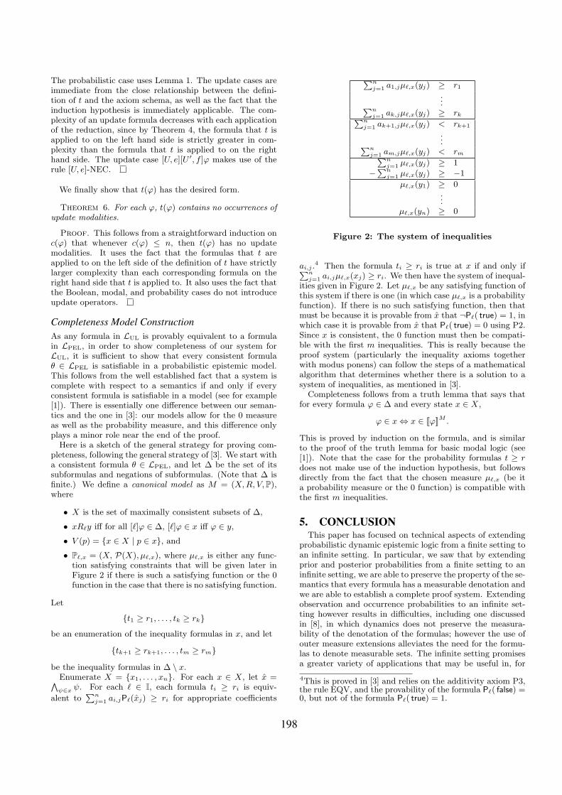
• P`,x = (X, P(X), µ`,x), where µ`,x is either any func-tion satisfying constraints that will be given later inFigure 2 if there is such a satisfying function or the 0function in the case that there is no satisfying function.

Let

{t1 ≥ r1, . . . , tk ≥ rk}be an enumeration of the inequality formulas in x, and let

{tk+1 ≥ rk+1, . . . , tm ≥ rm}be the inequality formulas in ∆ \ x.

Enumerate X = {x1, . . . , xn}. For each x ∈ X, let x̂ =Vψ∈x ψ. For each ` ∈ I, each formula ti ≥ ri is equiv-

alent toPnj=1 ai,jP`(x̂j) ≥ ri for appropriate coefficients

Pnj=1 a1,jµ`,x(yj) ≥ r1

...Pnj=1 ak,jµ`,x(yj) ≥ rkPn

j=1 ak+1,jµ`,x(yj) < rk+1

...Pnj=1 am,jµ`,x(yj) < rmPn

j=1 µ`,x(yj) ≥ 1

−Pnj=1 µ`,x(yj) ≥ −1

µ`,x(y1) ≥ 0...

µ`,x(yn) ≥ 0

Figure 2: The system of inequalities

ai,j .4 Then the formula ti ≥ ri is true at x if and only ifPn

j=1 ai,jµ`,x(xj) ≥ ri. We then have the system of inequal-ities given in Figure 2. Let µ`,x be any satisfying function ofthis system if there is one (in which case µ`,x is a probabilityfunction). If there is no such satisfying function, then thatmust be because it is provable from x̂ that ¬P`( true) = 1, inwhich case it is provable from x̂ that P`( true) = 0 using P2.Since x is consistent, the 0 function must then be compati-ble with the first m inequalities. This is really because theproof system (particularly the inequality axioms togetherwith modus ponens) can follow the steps of a mathematicalalgorithm that determines whether there is a solution to asystem of inequalities, as mentioned in [3].

Completeness follows from a truth lemma that says thatfor every formula ϕ ∈ ∆ and every state x ∈ X,

ϕ ∈ x⇔ x ∈ [[ϕ]]M .

This is proved by induction on the formula, and is similarto the proof of the truth lemma for basic modal logic (see[1]). Note that the case for the probability formulas t ≥ rdoes not make use of the induction hypothesis, but followsdirectly from the fact that the chosen measure µ`,x (be ita probability measure or the 0 function) is compatible withthe first m inequalities.

5. CONCLUSIONThis paper has focused on technical aspects of extending

probabilistic dynamic epistemic logic from a finite setting toan infinite setting. In particular, we saw that by extendingprior and posterior probabilities from a finite setting to aninfinite setting, we are able to preserve the property of the se-mantics that every formula has a measurable denotation andwe are able to establish a complete proof system. Extendingobservation and occurrence probabilities to an infinite set-ting however results in difficulties, including one discussedin [8], in which dynamics does not preserve the measura-bility of the denotation of the formulas; however the use ofouter measure extensions alleviates the need for the formu-las to denote measurable sets. The infinite setting promisesa greater variety of applications that may be useful in, for

4This is proved in [3] and relies on the additivity axiom P3,the rule EQV, and the provability of the formula P`( false) =0, but not of the formula P`( true) = 1.

198

example, robotics, where there is uncertainty in measure-ments over infinitely many possible values. We, however,leave such applications to future work. Other interesting di-rections of research include the study of the complexity ofthe logics, possible connections with the rich body of thetheory of coalgebraic modal logics, and the development ofmodel checking tools for this logic.

6. ACKNOWLEDGEMENTSLuca Aceto, Anna Ingolfsdottir and Joshua Sack have

been partially supported by the project ‘Processes and ModalLogics’ (project nr. 100048021) of the Icelandic Fund for Re-search. The work on the paper was partly carried out whileLuca Aceto and Anna Ingolfsdottir held Abel ExtraordinaryChairs at Universidad Complutense de Madrid, Spain, sup-ported by the NILS Mobility Project.

7. REFERENCES[1] P. Blackburn, M. de Rijke, and Y. Venema. Modal

logic. Cambridge University Press, New York, NY,USA, 2001.

[2] H. v. Ditmarsch, W. van der Hoek, and B. Kooi.Dynamic Epistemic Logic. Springer PublishingCompany, Incorporated, 1st edition, 2007.

[3] R. Fagin and J. Y. Halpern. Reasoning aboutknowledge and probability. In Proceedings of the 2ndconference on Theoretical aspects of reasoning aboutknowledge, TARK ’88, pages 277–293, San Francisco,CA, USA, 1988. Morgan Kaufmann Publishers Inc.

[4] R. Gariepy and W. Ziemer. Modern Real Analysis.PWS Publishing Company, Boston, MA, USA, 1995.

[5] B. P. Kooi. Probabilistic dynamic epistemic logic.Journal of Logic, Language and Information,12:381–408, 2003. 10.1023/A:1025050800836.

[6] B. Renne, J. Sack, and A. Yap. Dynamic epistemictemporal logic. In X. He, J. Horty, and E. Pacuit,editors, Logic, Rationality, and Interaction, volume5834 of Lecture Notes in Computer Science, pages263–277. Springer Berlin / Heidelberg, 2009.10.1007/978-3-642-04893-7 21.

[7] B. Renne, J. Sack, and A. Yap. Dynamic epistemictemporal logic. Extended manuscript, 2009.

[8] J. Sack. Extending probabilistic dynamic epistemiclogic. Synthese, 169:241–257, 2009.10.1007/s11229-009-9555-3.

[9] J. Sack. Logic for update products and steps into thepast. Annals of Pure and Applied Logic, 161(12):1431– 1461, 2010.

[10] J. van Benthem, J. Gerbrandy, and B. Kooi. Dynamicupdate with probabilities. Studia Logica, 93:67–96,2009. 10.1007/s11225-009-9209-y.

199