arX

iv:0

906.

4225

v6 [

mat

h.O

A]

14

Apr

201

1

A2-Planar Algebras I

David E. Evans and Mathew Pugh

School of Mathematics,Cardiff University,

Senghennydd Road,Cardiff, CF24 4AG,

Wales, U.K.

April 15, 2011

Abstract

We give a diagrammatic presentation of the A2-Temperley-Lieb algebra. Gen-eralizing Jones’ notion of a planar algebra, we formulate an A2-planar algebra mo-tivated by Kuperberg’s A2-spider. This A2-planar algebra contains a subfamily ofvector spaces which will capture the double complex structure pertaining to thesubfactor for a finite SU(3) ADE graph with a flat cell system, including both theperiodicity three coming from the A2-Temperley-Lieb algebra as well as the pe-riodicity two coming from the subfactor basic construction. We use an A2-planaralgebra to obtain a description of the (Jones) planar algebra for the Wenzl subfactorin terms of generators and relations.

Mathematics Subject Classification 2010: Primary 46L37; Secondary 46L60, 81T40.

1 Introduction

A braided inclusion N ⊂ M , where there is a braided system of SU(3)k endomorphisms

NXN on the factor N , yields a nimrep (non-negative integer matrix representation) ofthe right action of the N -N sectors NXN on the M-N sectors MXN via the theory ofα-induction [9, 10, 11]. This nimrep defines a classifying graph G, which is of ADE type.One can build an Ocneanu cell system W on an ADE graph G [54], which attaches acomplex number to each closed path of length three on the edges of G. A cell systemW naturally gives rise to a representation of the Hecke algebra, or more precisely, of theA2-Temperley-Lieb algebra [21, 22], which is a quotient of the Hecke algebra given bythe fixed point algebra of

⊗NM3 under the action of SU(3)k. This A2-Temperley-Lieb

algebra has an inherent periodicity of three coming from the representation theory ofSU(3).

To each pair (G,W ), consisting of an SU(3) ADE graph G and a cell system W on G,there is associated a subfactor N ⊂M , or rather, a subfactor double complex (c.f. [19]),

1

which has a periodicity of three in the horizontal direction, coming from the A2-Temperley-Lieb algebra, and a periodicity of two in the vertical direction, coming from the subfactorbasic construction of Jones [30], or equivalently, from the (usual) Temperley-Lieb algebra.The subfactor double complex contains the tower of higher relative commutants N ′ ⊂Mi

as its initial column, where N ⊂ M ⊂ M1 ⊂ M2 . . . is the tower obtained by iteratingthe basic construction. However, it also contains the SU(3) structure captured by theA2-Temperley-Lieb operators, which is lost in the tower of higher relative commutants,or indeed in the standard invariant.

The main goal of this paper is to provide a framework for an A2 version of a planaralgebra which describes the subfactor double complex. We begin by giving a diagrammaticpresentation of the A2-Temperley-Lieb algebra, consisting of A2-tangles which are a specialclass of Kuperberg’s A2 webs [44]. The A2-Temperley-Lieb algebra is the underlyingalgebra in our A2-planar algebra, which is a family of vector spaces which carry an actionof the A2-tangles.

The main result of the paper is Theorem 6.4, where for any pair (G,W ) we explicitlyassociate to the corresponding subfactor double complex an A2-planar algebra, that is,there is an action of the A2-tangles on each finite-dimensional vector space in the subfactordouble complex. As an immediate corollary we obtain a description of the (usual) planaralgebra for Wenzl’s Hecke subfactor in terms of generators and relations [70]. This workprovides a framework for studying subfactor double complexes, even in the continuousSU(3) regime beyond index nine.

2 Preliminaries

A subfactor encodes symmetries. These can be understood and studied from a numberof vantage points and directions which have interlocking ideas. In a subfactor’s mostfundamental setting, these symmetries may arise from a group, a group dual or a Hopfalgebra, and their actions on a von Neumann algebraM , but subfactor symmetries go farbeyond this, and beyond quantum groups. The symmetries of a group G and group dualmay be recovered from the position of the fixed point algebra MG in the ambient algebraM and the position of M in the crossed product M ⋊ G. More generally, the symmetryor quantum symmetry is encoded by the position of a von Neumann algebra in another.Subfactors encode data, algebraic, combinatorial and analytic, and the question arises asto how to recover the data from the subfactor N ⊂M and vice versa.

Iterating the basic construction of Jones [30] in the type II1 setting, one obtains a towerN ⊂ M ⊂ M1 ⊂ M2 . . . . The standard invariant is obtained by considering the towerof relative commutants M ′

i ∩Mj , which are finite dimensional in the case of finite index.Different axiomatizations of the standard invariant are given by Ocneanu with paragroups[51], emphasising connections and their flatness, and by Popa with λ-lattices and a moreprobabilistic language which permit reconstruction of the (extremal finite index) subfactorunder certain amenable conditions [60]. Jones [31] produced another formulation usingplanar algebras, a diagrammatic incarnation of the relative commutants, closed underplanar contractions or carrying operations indexed by certain planar diagrams, such thatany extremal subfactor gives a planar algebra. Conversely, using the work of Popa onλ-lattices, every planar algebra, with suitable positivity properties, produces an extremal

2

finite index subfactor. Recent work of [28], this time with a free probabilistic input ofideas, has recovered the characterisation of Popa.

The most fundamental symmetry of a subfactor is through the Temperley Lieb algebra[68]. The Jones basic construction Mi−1 ⊂ Mi ⊂ Mi+1 is through adjoining an extraprojection ei arising from the projection or conditional expectation of Mi onto Mi−1.These projections satisfy the Temperley-Lieb relations of integrable statistical mechanics.They are contained in the tower of relative commutants of any finite index subfactor andare in some sense the minimal symmetries. The planar algebra of a subfactor also has toencode what else is there, but in the case of the Temperley-Lieb algebra its planar algebracorresponds to Kauffman’s diagrammatic presentation of the Temperley-Lieb algebra.The Temperley-Lieb algebra has a realization from SU(2), from the fixed point algebrasof quantum SU(2) on the Pauli algebra and special representations of Hecke algebrasof type A. These SU(2) subfactors generalize to SU(3) (and beyond [70, 69]). Thesesubfactors can be used to understand SU(3) orbifold subfactors, conformal embeddingsand modular invariants [19, 71, 9, 10, 11, 22].

Here we give a planar study of subfactors which encodes the representation theoryof quantum SU(3) diagrammatically. The Temperley-Lieb algebra is then generalized tothe following. The Hecke algebra Hn(q), q ∈ C, is the algebra generated by invertibleoperators gj, j = 1, 2, . . . , n− 1, satisfying the relations

(q−1 − gj)(q + gj) = 0, (1)

gigj = gjgi, |i− j| > 1, (2)

gigi+1gi = gi+1gigi+1. (3)

When q = 1, the first relation becomes g2j = 1, so that Hn(1) reduces to the group ring ofthe symmetric, or permutation, group Sn, where gj represents a transposition (j, j + 1).Writing gj = q−1 − Uj where |q| = 1, and setting δ = q + q−1, these generators andrelations lead to self-adjoint operators 1, U1, U2, . . . , Un−1 and relations

H1:

H2:

H3:

U2i = δUi,

UiUj = UjUi, |i− j| > 1,

UiUi+1Ui − Ui = Ui+1UiUi+1 − Ui+1,

where δ = q + q−1.To any σ in the permutation group Sn, decomposed into transpositions of nearest

neighbours σ =∏

i∈Iστi,i+1, we associate the operator gσ =

∏i∈Iσ

gi, which is well definedbecause of the braiding relation (3). Then the commutant of the quantum group SU(N)qis obtained from the Hecke algebra by imposing an extra condition, which is the vanishingof the q-antisymmetrizer [17] ∑

σ∈Sn

(−q)|Iσ|gσ = 0. (4)

For SU(2) it reduces to the Temperley-Lieb condition UiUi±1Ui−Ui = 0, whilst for SU(3)it is

(Ui − Ui+2Ui+1Ui + Ui+1) (Ui+1Ui+2Ui+1 − Ui+1) = 0. (5)

3

The A2-Temperley-Lieb algebra will be the algebra generated by a family {Un} of self-adjoint operators which satisfy the Hecke relations H1-H3 and the extra condition (5)(c.f. [47, 15]). The A2-Temperley-Lieb algebra is the fixed point algebra of

⊗NM3 under

the product action of⊗

NAd(ρ) of SU(3) or its quantum version SU(3)q. There is an

inherent periodicity three which comes from the representation theory of SU(3), whichis reflected in the Bratteli diagram of the McKay graph of the fusion of the fundamentalrepresentation. For q a kth root of unity or q = 1, the A2-Temperley-Lieb algebra isisomorphic to the path algebra of the SU(3) graph A(k+3), where k = ∞ for q = 1, whichis tripartite, or three-colourable, so that all closed paths on A(k+3) have lengths which aremultiples of three.

2.1 Background on Jones’ planar algebras

Jones introduced the notion of a planar algebra in [31] to study subfactors. Let us brieflyreview the essential construction of Jones’ planar algebras. A planar k-tangle consists ofa disc D in the plane with 2k vertices on its boundary, k ≥ 0, and n ≥ 0 internal discsDj, j = 1, . . . , n, where the disc Dj has 2kj vertices on its boundary, kj ≥ 0. One vertexon the boundary of each disc (including the outer disc D) is chosen as a marked vertex,and the segment of the boundary of each disc between the marked vertex and the verteximmediately adjacent to it as we move around the boundary in an anti-clockwise directionis labelled either + or −. For a disc which has no vertices on its boundary, we label itsentire boundary by + or −. Inside D we have a collection of disjoint smooth curves, calledstrings, where any string is either a closed loop, or else has as its endpoints the verticeson the discs, and such that every vertex is the endpoint of exactly one string. Any tanglemust also allow a checkerboard colouring of the regions inside D, which are bounded bythe strings and the boundaries of the discs, where every region is coloured black or whitesuch that any two regions which share a common boundary are not coloured the same, andany region which meets the boundary of a disc at the segment marked +, − is colouredblack, white respectively.

A planar k-tangle with an internal disc Dj with 2kj vertices on its boundary can becomposed with a kj-tangle S, giving a new k-tangle T ◦jS, by inserting the tangle S insidethe inner disc Dj of T such that the vertices on the outer disc of S coincide with thoseon the disc Dj, and in particular the two marked vertices must coincide. The boundaryof the disc Dj is then removed, and the strings are smoothed if necessary. The collectionof all diffeomorphism classes of such planar tangles, with composition defined as above,is called the planar operad.

A planar algebra P is then defined to be an algebra over this operad, i.e. a familyP = (P+

k , P−k ; k ≥ 0) of vector spaces with P±

k ⊂ P±k′ for k < k′, and with the following

property. For every k-tangle T with n internal discs Dj labelled by elements xj ∈ Pkj ,j = 1, . . . , n, there is an associated linear map Z(T ) : ⊗n

j=1Pkj → Pk, which is compatiblewith the composition of tangles and re-ordering of internal discs.

These planar algebras gave a topological reformulation of the standard invariant, de-scribed in terms of relative commutants in the standard tower of a subfactor. Moreprecisely, the standard invariant of an extremal subfactor N ⊂M is a (subfactor) planaralgebra P = (Pk)k≥0 with Pk = N ′ ∩ Mk−1. Conversely, every planar algebra can berealised by a subfactor [60, 31] (see also [28, 36, 41]). The index [30] is a crude measure

4

of the complexity of a subfactor – those subfactors with index < 4 being the simplest.Since every relative commutant contains the Temperley-Lieb algebra, another notion ofcomplexity is the number of non-Temperley-Lieb elements that are required to generatethe relative commutants. In the planar algebra set-up, planar algebras P generated bya single element, for which the dimension of P3 is at most 13, were classified in [8]. Inthe recent work of [42] it was shown that any subfactor planar algebra P of depth k isgenerated by a single element in Pt, for some t ≤ k + 1.

In [33] Jones studied annular tangles, that is, tangles with a distinguished internal disc.He introduced the notion of modules over a planar algebra, which are modules over an an-nular category whose morphisms are given by such annual tangles, and gave a descriptionof all irreducible Temperley-Lieb modules. A more general planar algebra is the graphplanar algebra of a bipartite graph [32]. Jones and Reznikoff obtained the decompositionof the graph planar algebras for the ADE graphs into irreducible Temperley-Lieb modules[33, 64]. A similar notion to an tangle is that of an affine tangle. Affine Temperley-Liebalgebras were studied in [35, 65].

One way to construct planar algebras is by generators and relations. One problem thatarises with this method is to determine whether or not a set of generators and relationswill produce a finite dimensional planar algebra, that is, a planar algebra P where eachPk, k > 0, is finite-dimensional. Landau [45] obtained a condition called an exchangerelation, which guarantees that a planar algebra is in fact finite dimensional, and thiscondition was extended and generalized in [26]. A bigger problem is to show whether ornot the trace defined on the planar algebra is positive definite. The graph planar algebrashave a positive definite trace. A recently published result in [34, Corollary 4.2] says thatevery finite-depth subfactor planar algebra is a planar subalgebra of the graph planaralgebra of its principal graph. If a planar algebra can be found as a planar subalgebra ofa graph planar algebra then the trace it inherits from the graph planar algebra will beautomatically positive definite. This motivated the construction of the planar algebra forthe ADE subfactors in terms of generators and relations [4, 49], and more recently for theHaagerup subfactor [58], and the extended Haagerup subfactor [5] where planar algebraswere used to show the existence of the extended Haagerup subfactor for the first time.

The planar algebras associated to different constructions of subfactors have been de-scribed: the planar algebra associated to subfactors arising from the outer actions on afactor by a finite-dimensional Kac algebra [39], by a semisimple and cosemisimple Hopfalgebra [40] and more recently by the actions of finite groups or finitely generated, count-able, discrete groups [27, 29, 6, 7]. Planar algebras associated to the action of compactquantum groups on finite quantum spaces were studied in [2].

3 Taking Jones’ planar algebras to the A2 setting

Our planar description naturally begins in this section with the spiders of Kuperberg[44] who developed some of the basic diagrammatics of the representation theory of A2

and other rank two Lie algebras. Here we give a diagrammatic presentation of the A2-Temperley-Lieb algebra using Kuperberg’s A2 spider, and show that the A2-Temperley-Lieb algebra is isomorphic to Wenzl’s quotient of the Hecke algebra [70]. In Section 4we introduce and study the notion of a general A2-planar algebra and in Section 4.3

5

the notion of an A2-planar algebra and the notion of flatness. In Section 5 we describeparticular subspaces that we are interested in, which will correspond exactly to the doublecomplex associated to the SU(3)-subfactors.

The SU(3) ADE graphs appear as nimreps for the SU(3) modular invariants [21, 22].For each graph there is a construction of a subfactor via a double complex of finite-dimensional algebras (cf. λ-lattice in what one could call the SU(2) setting) which relieson the existence of a cell system which defines a connection or Boltzmann weight. Theseries of the commuting squares in these double complexes are not canonical in the sense ofPopa, because although these double complexes have period 2 vertically (coming from thesubfactor basic construction) they have period 3 horizontally (coming from the underlyingA2-Temperley-Lieb algebraic structure). These double complexes were used by Evans andKawahigashi [19] to understand the Wenzl subfactors and their orbifolds, and in particularto compute their principal graphs. The main result of the paper is Theorem 6.4 in Section6, where we show how the subfactor, or associated double complex, for a finite ADEgraph with a flat cell system diagrammatically gives rise to a flat A2-C

∗-planar algebra.Jones’ (A1-)planar algebra is contained in the A2-planar algebra, as the algebra over acertain suboperad of our A2-planar operad. In Section 6.2 we obtain an A2-planar algebradescription of the Wenzl subfactor, and as a corollary we have a construction of Jones’planar algebra for the Wenzl subfactor in terms of generators and relations which comefrom the A2-planar algebra.

In [21] we computed the numerical values of the Ocneanu cells, announced by Ocneanu(e.g. [54, 55]), and consequently representations of the Hecke algebra, for the SU(3) ADEgraphs. These cells assign a numerical weight to Kuperberg’s diagram of trivalent vertices– corresponding to the fact that the trivial representation is contained in the triple productof the fundamental representation of SU(3) through the determinant. They will yield, ina natural way, representations of an A2-Temperley-Lieb or Hecke algebra. For bipartitegraphs, the corresponding weights (associated to the diagrams of cups or caps), arisein a more straightforward fashion from a Perron-Frobenius eigenvector, giving a naturalrepresentation of the Temperley-Lieb algebra or Hecke algebra.

In the sequel [23] we introduce the notion of modules over an A2-planar algebra, anddescribe certain irreducible Hilbert A2-TL-modules. A partial decomposition of graphA2-planar algebras for the ADE graphs is achieved. The graph A2-planar algebra P

G ofan ADE graph is an A2-C

∗-planar algebra with dim(P G0 ) > 1, which is a generalization of

the bipartite graph planar algebra to the A2 setting. These graph A2-planar algebras arediagrammatic representations of another double complex of finite dimensional algebras,where now the initial space in the double complex is Cn where n > 1 (note that n = 1 forthe initial space in the double complex associated to an SU(3)-subfactor).

The bipartite theory of the SU(2) setting has to some degree become a three-colourabletheory in our SU(3) setting. This theory is not completely three-colourable since someof the graphs are not three-colourable – namely the graphs A(n)∗ associated to the con-jugate modular invariants, n ≥ 4, D(n) associated to the orbifold modular invariants,n 6= 0 mod 3, and the exceptional graph E (8)∗. The figures for the complete list of theADE graphs are given in [3, 21].

We have laid the foundations for a planar algebra formulation of an SU(3) theory whichmay help resolve some of the unanswered questions left open in the programme which weset out on in [21, 22] to understand SU(3) modular invariants and their representation by

6

braided subfactors. We realised all SU(3) modular invariants by braided SU(3) subfactors[22] but did not classify their associated nimreps or claim that the known list is exhaustive.In the case of one of the exceptional modular invariants, we could not identify the nimrep.We verified that all known candidate nimrep graphs carried Ocneanu cell systems [21],

apart from one exceptional graph E(12)4 . However, we did not determine when such a cell

system yields a local braided subfactor, but speculated that this should correspond totype I cell systems, that is, cell systems such that the connection defined by equations(20), (21) in the present paper is flat. This is only known for the A and D graphs atpresent [19].

The question of whether all nimreps have been realised is open. There are somenimreps which do not have braided subfactors. We also want to go beyond the ADEclassification to study subfactors for more exotic graphs which support a cell system, justas Jones’ planar algebras facilitated the study of the Haagerup and extended Haagerupsubfactors. The tools being drawn up in this paper may aid these further studies.

3.1 Orbifolds

The orbifold construction is a standard procedure in operator algebras, in C∗-algebras andsubfactor theory in von Neumann algebras, as well as in integrable statistical mechanicsand conformal field theory. A finite abelian group action on the underlying structure canbring about an orbifold, by suitably dividing out by the group elements (usually calledsimple currents in conformal field theory) which may or may not describe completelydifferent theory from the original one. This usually depends on having fixed points, andunderstanding their role or the resolution of these singularities is the key.

For example, in the theory of C∗-algebras, the fixed point algebra of the irrationalrotation algebra by a flip on the generators or the underlying two dimensional torus hasan AF fixed point algebra, and so has a completely different character to the ambientnoncommutative torus which has non trivial K1. This is reviewed with full referencesin [20, notes to Ch.3, pp 125–146]. The invariants involved in understanding or com-paring orbifolds, the fixed point algebras or crossed products, with the original algebrasbeing K-theory or equivariant K-theory. Partly motivated by this, orbifold methods wereintroduced into subfactor theory [19], but first we digress to the underlying statisticalmechanics and conformal field theories.

In statistical mechanics, Date, Jimbo, Miwa and Okado [16] introduced integrablemodels associated with the level k-integrable models of the Kac-Moody algebra of SU(n).The Boltzmann weights lie in the fixed point algebra of the infinite tensor product of Mn

under the action of SU(n)k.The notion of an orbifold of such a model by dividing out by a subgroup Z of the centre

of SU(n) were introduced by Pasquier [57], Fendley and Ginsparg [24] for n = 2 and byDi-Franceso and Zuber [17] for n = 3, borrowing from an orbifold notion in conformal fieldtheory [18]. In the Wess-Zumino-Witten model, a two dimensional conformal field theoryarises from classical fields taking values in the target SU(n) models and their orbifoldsby Z are meant to be those living in the quotient SU(n)/Z.

With all this mind, the orbifold construction was introduced in subfactor theory in[19], with the Boltzmann weights being in the relevant fixed point algebras and hencenaturally satisfy the Yang-Baxter equation, and the subfactors introduced through the

7

action of the subgroup Z of the centre as a group of automorphisms and crossed products.It is still a question whether one is really finding a new subfactor, as in the N = 2 case,one cannot simply take the orbifold of the A4m−1-principal graph which would be D2m+1,as only Dm for m even can arise as a principal graph of a subfactor. For the SU(3)subfactor the action of the center Z3 of SU(3) introduces an action for each integer levelk on NXN , a system of endomorphisms of a type III factor N represented by the verticesof the truncated diagram A(k+3).

These orbifolds are best understood through α-induction in subfactor theory [10, Sec-tion 3], [11, Section 6.2], [12, Section 8], which we summarize here.

Simple currents [66] are primary fields with unit quantum dimension and appear inthe subfactor framework as automorphisms in the system NXN . They form a closedabelian group under fusion. Simple currents give rise to modular invariants, and all suchinvariants have been classified [25, 43]. We are focussing on SU(n) here for n = 2, 3, andso will only consider cyclic simple current groups Zn.

By taking a generator [σ] of the cyclic simple current group Zn we can construct thecrossed product subfactor N ⊂ M = N ⋊ Zn whenever we can choose a representative σin each such simple current sector such that we have exact cyclicity σn = 1 (and not onlyas sectors). Rehren’s lemma [63] states that such a choice is possible if and only if thestatistics phase ωσ is an n-th root of unity, i.e. if and only if the conformal weight hσ is aninteger multiple of 1/n. This construction gives rise to a non-trivial subfactor and in turnto a modular invariant. For SU(n)k the simple current group Zn corresponds to weightskΛ(j), j = 0, 1, ..., n− 1. The conformal dimensions are hkΛ(j)

= kj(n − j)/2n, which byRehren’s Lemma [63] allow for full Zn extensions except when n is even and k is odd inwhich case the maximal extension is N ⊂ M = N ⋊ Zn/2 because we can only use theeven labels j. (This reflects the fact that e.g. for SU(2) there are no D-invariants at oddlevels.) Thus Rehren’s lemma has told us that extensions are labelled by all the divisorsof n unless n is even and k is odd in which case they are labelled by the divisors of n/2.This matches exactly the simple current modular invariant classification of [25, 43]. Anextension by a simple current subgroup Zm, with m a divisor of n or n/2, is moreoverlocal, if the generating current (and hence all in the Zm subgroup) has integer conformalweight, hkΛ(q)

∈ Z, where n = mq. This happens exactly if kq ∈ 2mZ if n is even, orkq ∈ mZ if n is odd [11]. For SU(2) this corresponds to the Deven series whereas the Dodd

series are non-local extensions. For SU(3), there is a simple current extension at eachlevel, but only those at k ∈ 3Z are local. For the case of SU(3) at level 3p, the crossedproduct N ⊂ N ⋊ Z3 with canonical endomorphism [θ] = [λ(0,0)]⊕ [λ(3p,0)]⊕ [λ(0,3p)], theprocedure of alpha induction [10, p.89] yields from 〈αλ, αµ〉 = 〈θλ, µ〉 that at the fixed

point f = (p, p), [αf ] = [α(1)f ]⊕ [α

(2)f ]⊕ [α

(3)f ] splits into three irreducibles whilst otherwise

[αλ] is irreducible and identified with [ασλ], σ ∈ Z3, under the action of the centre Z3 orsimple currents. Thus under alpha induction, the Verlinde algebra or the tensor categoryof SU(3) at level 3p, represented by a system of endomorphisms NXN is taken to itsorbifold NX

±N , and taking the dual action reverses this procedure. The principal graphs

(the fusion graphs of [α(1,0)]) are the orbifold graphs D3p+3.Muger [50] and Bruguieres [14] have subsequently introduced an orbifold procedure

which can handle non abelian groups, and this procedure is sometimes described as equiv-ariantization/deequivariantization in the category oriented literature. We pointed out in[21] recent work in condensed matter physics [1] where we see that α-induction is playing

8

Figure 1: A2 webs

a key role. For example, the computation of pages 8–9 is α-induction for an orbifoldembedding of SU(2)4 which gives fusion graph D4. Other examples are the conformalembedding of SU(2)4 ⊂ SU(3)1 on pages 14–15, which again gives fusion graph D4, andthe conformal embedding SU(2)10 ⊂ SO(5)1 on pages 15–16, which gives fusion graphE6.

3.2 A2-tangles

In [44], Kuperberg defined the notion of a spider, which is an axiomatization of therepresentation theory of groups and other group-like objects. The invariant spaces havebases given by certain planar graphs. These graphs are called webs, hence the term spider.In [44] certain spiders were defined in terms of generators and relations, isomorphic tothe representation theories of rank two Lie algebras and the quantum deformations ofthese representation theories. This formulation generalized a well-known construction forA1 = su(2) by Kauffman [37].

For the A2 = su(3) case, we have the A2 webs, illustrated in Figure 1. We willcall these webs incoming and outgoing trivalent vertices respectively. We call theoriented lines strings. We may join the A2 webs together by attaching free ends ofoutgoing trivalent vertices to free ends of incoming trivalent vertices, and isotoping thestrings if needed so that they are smooth.

We are now going to systematically define an algebra of web tangles, and express thisin terms of generators and relations.

Definition 3.1 An A2-tangle will be a connected collection of strings joined together atincoming or outgoing trivalent vertices (see Figure 1), possibly with some free ends, suchthat the orientations of the individual strings are consistent with the orientations of thetrivalent vertices.

Definition 3.2 We call a vertex a source vertex if the string attached to it has orien-tation away from the vertex. Similarly, a sink vertex will be a vertex where the stringattached has orientation towards the vertex.

Definition 3.3 Form,n ≥ 0, an A2-(m,n)-tangle will be an A2-tangle T on a rectangle,where T has m+ n free ends attached to m source vertices along the top of the rectangleand n sink vertices along the bottom such that the orientation of the strings is respected.If m = n we call T simply an A2-m-tangle, and we position the vertices so that for everyvertex along the top there is a corresponding vertex directly beneath it along the bottom.

Two A2-(m,n)-tangles are equivalent if one can be obtained from the other by anisotopy which moves the strings and trivalent vertices, but leaves the boundary verticesunchanged. We define T A2

m,n to be the set of all (equivalence classes of) A2-(m,n)-tangles.

9

The composition TS ∈ T A2m,k of an A2-(m,n)-tangle T and an A2-(n, k)-tangle S is

given by gluing S vertically below T such that the vertices at the bottom of T and thetop of S coincide, removing these vertices, and isotoping the glued strings if necessary tomake them smooth. The composition is clearly associative.

Definition 3.4 We define the vector space VA2m,n to be the free vector space over C with

basis T A2m,n. Then VA2

m,n has an algebraic structure with multiplication given by compositionof tangles. In particular, we will write VA2

m for VA2m,m, and VA2 =

⋃m≥0 V

A2m . For n < m

we have VA2n ⊂ VA2

m , with the inclusion of an n-tangle T ∈ T A2n in T A2

m given by addingm− n vertices along the top and bottom of the rectangle after the rightmost vertex, withm − n downwards oriented vertical strings connecting the extra vertices along the top tothose along the bottom. The inclusion for VA2

n in VA2m is the linear extension of this map.

Note that T A2m,n is infinite, and thus the vector space VA2

m,n is infinite dimensional.However, we will take a quotient of VA2

m,n which will turn out to be finite dimensional. LetK1-K3 denote the following relations on local parts of tangles, for α, δ ∈ C [44]:

K1:

K2:

K3:

Definition 3.5 We define Im,n ⊂ VA2m,n to be the ideal of VA2

m,n which is the linear span ofthe relations K1-K3.

By the linear span of the relations K1-K3 is meant the linear span of the differencesof the left hand side and the right hand side of each of the relations, as local parts of thetangles, where the rest of the tangle is identical in each term in the difference. We willdenote Im,m by Im. Note that Im ⊂ Im+1.

Definition 3.6 The algebra V A2m is defined to be the quotient of the space VA2

m by the idealIm, and V

A2 =⋃

m≥0 VA2m .

A basis of V A2m is given by all A2-m-tangles which do not contain the local pictures

which appear on the left hand side of K1-K3 (which Kuperberg calls elliptic faces). We

will call the local picture a digon, and an embedded square. We couldreplace the Kuperberg relation K1 by the more general relations:

K1’:

Although it now appears that we have three independent parameters α1, α1, δ, weactually have only one, as shown in the following Lemma:

10

Figure 2: 3-tangles B1, B2, E

Lemma 3.7 For a fixed complex number δ 6= 0 we must have either α1 = α2 = δ2 − 1 orα1 = α2 = 0.

Proof: Let B1 be the 3-tangle illustrated in Figure 2, which is the composition of threebasis tangles in V A2

3 . Let B2 be a 3-tangle which comes from a similar composition, andE a basis tangle in V A2

3 , both also illustrated in Figure 2. Reducing B1 using K2 twice,we get B1 = δ2E. On the other hand, if we reduce B1 using K3, we get an anticlockwiseoriented closed loop, which by K1’ contributes a scalar factor α1. Then we also haveB1 = E + α1E. If E 6= 0, then δ2 = 1 + α1, and by the same argument on B2 we alsoobtain δ2 = 1 + α2. Suppose now that E = 0. Let E be the tangle given by compositionof E (embedded in V A2

6 ) with three nested caps above and three nested cups below, i.e.

E is the tangle

If we use K2 to remove the left digon, we obtain an anticlockwise oriented loop, and sothe diagram counts as the scalar α1δ. If instead we used K2 to remove the right digon wewould obtain the scalar α2δ. Since E = 0 and δ 6= 0, we have α1 = α2 = 0. �

For m ∈ Z, we define the quantum integer [m]q by [m]q = (qm−q−m)/(q−q−1), whereq ∈ C. Note that if δ = [2]q, then by Lemma 3.7 α = δ2 − 1 = [3]q (or zero). When q isan nth root of unity, q = e2πi/n, we will usually write [m] for [m]q.

There is a braiding on V A2, defined locally by the following linear combinations oflocal diagrams in V A2 , for a choice of third root q1/3, q ∈ C (see [44, 67]):

(6)

(7)

11

The braiding satisfies the following properties locally, provided δ = [2]q and α = [3]q:

(8)

(9)

where we also have relation (9) with the crossings all reversed.We call the local pictures illustrated on the left hand sides of relations (6), (7) re-

spectively a negative, positive crossing respectively. With this braiding, kinks (or twists)contribute a scalar factor of q8/3 for those involving a positive crossing, and q−8/3 for thoseinvolving a negative crossing, as shown in Figure 3.

Figure 3: Removing kinks

We now define a ∗-operation on VA2m , which is an involutive conjugate linear map. For

an m-tangle T ∈ T A2m , T ∗ is the m-tangle obtained by reflecting T about a horizontal line

halfway between the top and bottom vertices of the tangle, and reversing the orientationson every string. Then ∗ on VA2

m is the conjugate linear extension of ∗ on T A2m . Note that

the ∗-operation leaves the relation K2 invariant if and only if δ ∈ R. For δ ∈ R, the∗-operation leaves the ideal Im invariant due to the symmetry of the relations K1-K3.Then ∗ passes to V A2

m , and is an involutive conjugate linear anti-automorphism.

3.3 Diagrammatic presentation of the A2-Temperley-Lieb alge-

bra

From now on we let δ be real, so that δ = [2]q for some q, and we set α = [3]q (cf. Lemma3.7). We define the tangle 1m to be the m-tangle with all strings vertical through strings.Then 1m is the identity of the algebra VA2

m : 1ma = a = a1m for all a ∈ VA2m . We also

define Wi to be the m-tangle with all vertices along the top connected to the vertices

along the bottom by vertical lines, except for the ith and (i + 1)th vertices. The strings

attached to the ith and (i + 1)th vertices along the top are connected at an incomingtrivalent vertex, with the third string coming from an outgoing trivalent vertex connected

to the strings attached to the ith and (i+1)th vertices along the bottom. The tangle Wi

is illustrated in Figure 4.For m ∈ N ∪ {0} we define the algebra A2-TLm to be alg(1m, wi|i = 1, . . . , m − 1),

where wi = Wi+Im. The wi’s in A2-TLm are clearly self-adjoint, and satisfy the relationsH1-H3, as illustrated in Figures 5, 6 and 7.

12

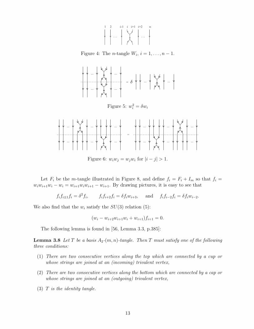
Figure 4: The n-tangle Wi, i = 1, . . . , n− 1.

Figure 5: w2i = δwi

Figure 6: wiwj = wjwi for |i− j| > 1.

Let Fi be the m-tangle illustrated in Figure 8, and define fi = Fi + Im so that fi =wiwi+1wi − wi = wi+1wiwi+1 − wi+1. By drawing pictures, it is easy to see that

fifi±1fi = δ2fi, fifi+2fi = δfiwi+3, and fifi−2fi = δfiwi−2.

We also find that the wi satisfy the SU(3) relation (5):

(wi − wi+2wi+1wi + wi+1)fi+1 = 0.

The following lemma is found in [56, Lemma 3.3, p.385]:

Lemma 3.8 Let T be a basis A2-(m,n)-tangle. Then T must satisfy one of the followingthree conditions:

(1) There are two consecutive vertices along the top which are connected by a cup orwhose strings are joined at an (incoming) trivalent vertex,

(2) There are two consecutive vertices along the bottom which are connected by a cap orwhose strings are joined at an (outgoing) trivalent vertex,

(3) T is the identity tangle.

13

Figure 7: wiwi+1wi − wi = wi+1wiwi+1 − wi+1

Figure 8: The n-tangle Fi, i = 1, . . . , n− 2.

Thus for any basis A2-m-tangle which is not the identity tangle, there must be two(consecutive) vertices along the top or bottom whose strings are joined at an incomingor outgoing trivalent vertex respectively. In fact, by a Euler characteristic argument, thismust be true for two vertices along both the top and bottom.

Then we have the following lemma which says that the A2-Temperley-Lieb algebraA2-TL is equal to the algebra V A2 of all A2-tangles subject to the relations K1-K3. This isthe A2 analogue of the fact that the Temperley-Lieb algebra TLn = alg(1, e1, e2, . . . , en−1)is isomorphic to Kauffman’s diagram algebra [37], which is the algebra generated by theelements E1, E2, . . . , En−1 on n strings, illustrated in Figure 9, along with the identitytangle 1n where every vertex along the top is connected to a vertex along the bottom by

Figure 9: The n-diagram Ei, i = 1, . . . , n− 1

14

a vertical through string. This lemma appeared in [61], and also independently with analternate proof in [62, Theorem 2.2].

Lemma 3.9 The algebra V A2m is generated by 1m and Wi ∈ V A2

m , i = 1, . . . , m − 1. SoV A2m

∼= A2-TLm.

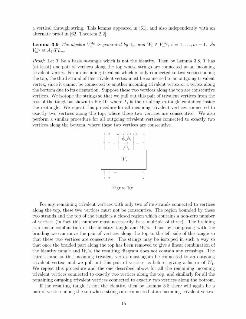
Proof: Let T be a basis m-tangle which is not the identity. Then by Lemma 3.8, T has(at least) one pair of vertices along the top whose strings are connected at an incomingtrivalent vertex. For an incoming trivalent which is only connected to two vertices alongthe top, the third strand of this trivalent vertex must be connected to an outgoing trivalentvertex, since it cannot be connected to another incoming trivalent vertex or a vertex alongthe bottom due to its orientation. Suppose these two vertices along the top are consecutivevertices. We isotope the strings so that we pull out this pair of trivalent vertices from therest of the tangle as shown in Fig 10, where T1 is the resulting m-tangle contained insidethe rectangle. We repeat this procedure for all incoming trivalent vertices connected toexactly two vertices along the top, where these two vertices are consecutive. We alsoperform a similar procedure for all outgoing trivalent vertices connected to exactly twovertices along the bottom, where these two vertices are consecutive.

Figure 10:

For any remaining trivalent vertices with only two of its strands connected to verticesalong the top, these two vertices must not be consecutive. The region bounded by thesetwo strands and the top of the tangle is a closed region which contains a non-zero numberof vertices (in fact this number must necessarily be a multiple of three). The braidingis a linear combination of the identity tangle and Wi’s. Thus by composing with thebraiding we can move the pair of vertices along the top to the left side of the tangle sothat these two vertices are consecutive. The strings may be isotoped in such a way sothat once the braided part along the top has been removed to give a linear combination ofthe identity tangle and Wi’s, the resulting diagram does not contain any crossings. Thethird strand at this incoming trivalent vertex must again be connected to an outgoingtrivalent vertex, and we pull out this pair of vertices as before, giving a factor of W1.We repeat this procedure and the one described above for all the remaining incomingtrivalent vertices connected to exactly two vertices along the top, and similarly for all theremaining outgoing trivalent vertices connected to exactly two vertices along the bottom.

If the resulting tangle is not the identity, then by Lemma 3.8 there will again be apair of vertices along the top whose strings are connected at an incoming trivalent vertex.

15

Figure 11: Tr(T ) Figure 12: Tr(ab) = Tr(ba)

Since all the incoming trivalent vertices which are connected to exactly two vertices alongthe top have been removed, this trivalent vertex must have all its strands connected tovertices along the top. By a similar argument there will also be an outgoing vertex whichis connected to three vertices along the bottom. Then using the braiding we move thispair of trivalent vertices to the left of the diagram, which gives a factor F1. Repeatingthis procedure we remove all the remaining trivalent vertices in the tangle, and we aredone. �

3.4 Trace on VA2

n

The following proposition is from [56, Prop. 1.2, p.375]:

Proposition 3.10 The quotient V A20 = A2-TL0 of the free vector space of all planar

0-tangles by the Kuperberg relations K1-K3 is isomorphic to C.

We define a trace Tr on VA2m as follows. For an A2-m-tangle T ∈ VA2

m , we form the0-tangle Tr(T ) as in Figure 11 by joining the last vertex along the top of T to the lastvertex along the bottom by a string which passes round the tangle on the right hand side,and joining the other vertices along the top to those on the bottom similarly. Then Tr(T )gives a value in C by Proposition 3.10. We could define the above trace as a right trace,and define a left trace similarly where the strings pass round the tangle on the left handside. However, by the comments after Proposition 4.7, the right and left traces are equal.The trace of a linear combination of tangles is given by linearity. Clearly Tr(ab) = Tr(ba)for any a, b ∈ VA2

m , as in Figure 12. For any x ∈ Im we have Tr(x) = 0, which followstrivially from the definition of Tr. Then Tr is well defined on V A2

m . We define a normalizedtrace tr on VA2

m by tr = α−mTr, so that tr(1m) = 1. Then tr is a Markov trace on V A2

since for x ∈ V A2

k , tr(Wkx) = δα−1tr(x), as illustrated in Figure 13, and in particulartr(Wi) = δα−1. The Markov trace tr is positive by Lemma 3.11 and [70, Theorem 3.6(b)].

Figure 13: Markov trace on V A2

16

For each non-negative integer m we define an inner-product on VA2m by

〈S, T 〉 = tr(T ∗S), (10)

which is well defined on V A2m since tr is.

For δ < 2 (so δ = [2]q = [2] where q = eπi/n, n ∈ N), we define V A2m to be the quotient

of V A2m by the zero-length vectors in V A2

m with respect to the inner-product defined in (10).Then the following lemma gives an identification between (a subalgebra of) the algebraof A2-tangles and ρ(H∞(q)) where ρ is one of Wenzl’s Hecke representations for SU(3)(see [70]). This lemma will be used later in Section 6.2.

Lemma 3.11 For δ ≥ 2, there is a C∗ representation ρ of H∞(q2) such that ρ(Hm(q2)) ∼=

V A2m . The representation ρ is equivalent to Wenzl’s representation π of the Hecke algebra,

and consequently V A2 is isomorphic to the path algebra for A(∞). For δ = [2]q, q = eπi/n,

there is a C∗ representation ρ of H∞(q2) such that ρ(Hm(q2)) ∼= V A2

m . In this case therepresentation ρ is equivalent to Wenzl’s representation π(3,n) of the Hecke algebra, andconsequently V A2 is isomorphic to the path algebra for A(n).

Proof: Clearly δ−1Wi, i = 1, . . . , m−1, is a self-adjoint projection in V A2m , and hence ρ is a

C∗-representation of Hm(q2) for any real q ≥ 1 or q = eπi/n. When q = ex, x ≥ 0, we have

η = (1−q2(−k+1))/(1+q2)(1−q−2k) = sinh((k−1)x)/2 cosh(x) sinh(kx) = [k−1]q/[2]q[k]q,whilst for q = eπi/n, η = sin((k − 1)π/n)/2 cos(π/n) sin(kπ/n) = [k − 1]/[2][k]. Then fork = 3, η = [3]−1

q so that the Markov trace on V A2m satisfies the condition in [70, Theorem

3.6]. �

Then the algebra V A2m is finite-dimensional for all finite m since the mth level of the

path algebra for A(n) is finite-dimensional.

4 A2-planar algebras

4.1 General A2-planar algebras

We will now define an A2-version of Jones’ planar algebra, using tangles generated by Ku-perberg’s A2-webs. Under certain assumptions, these A2-planar algebras will correspondto certain subfactors of SU(3) ADE graphs which have flat connections. The best way todescribe planar algebras is in terms of operads (see [31, 48]).

Definition 4.1 An operad consists of a sequence (C(n))n∈N of sets. There is a unitelement 1 in C(1), and a function C(n) ⊗ C(j1) ⊗ · · · ⊗ C(jn) → C(j1 + · · · + jn) calledcomposition, given by (y ⊗ x1 ⊗ · · · ⊗ xn) → y ◦ (x1 ⊗ · · · ⊗ xn), satisfying the followingproperties

• associativity: y ◦ (x1 ◦ (x1,1 ⊗ · · · ⊗ x1,k1)⊗ · · · ⊗ xn ◦ (xn,1 ⊗ · · · ⊗ xn,kn))= (y ◦ (x1 ⊗ · · · ⊗ xn)) ◦ (x1,1 ⊗ · · · ⊗ x1,k1 ⊗ · · · ⊗ xn,1 ⊗ · · · ⊗ xn,kn),

• identity: y ◦ (1⊗ · · · ⊗ 1) = y = 1 ◦ y.

17

Let σ = σ1 · · ·σm be a sign string, σj ∈ {±}. An A2-planar σ-tangle will be theunit disc D = D0 in C together with a finite (possibly empty) set of disjoint sub-discsD1, D2, . . . , Dn in the interior of D. Each disc Dk, k ≥ 0, will have mk ≥ 0 vertices on itsboundary ∂Dk, whose orientations are determined by sign strings σ(k) = σ

(k)1 · · ·σ

(k)mk where

‘+’ denotes a sink and ‘−’ a source, and such that the difference between the number of‘+’ and ‘−’ is 0 mod 3. The disc Dk will be said to have pattern σ(k). Inside D we havean A2-tangle where the endpoint of any string is either a trivalent vertex (see Figure 1)or one of the vertices on the boundary of a disc Dk, k = 0, . . . , n, or else the string formsa closed loop. Each vertex on the boundaries of the Dk is the endpoint of exactly onestring, which meets ∂Dk transversally. An example of an A2-planar σ-tangle is illustratedin Figure 14 for σ = −+−+−+−+.

Figure 14: A2-planar σ-tangle for σ = −+−+−+−+

The regions inside D have as boundaries segments of the ∂Dk or the strings. Theseregions ar labelled 0, 1 or 2, called the colouring, such that if we pass from a region Rof colour a to an adjacent region R′ by passing to the right over a vertical string withdownwards orientation, then R′ has colour a+ 1 (mod 3). We mark the segment of each∂Dk between the last and first vertices with ∗bk , bk ∈ {0, 1, 2}, so that the region insideD which meets ∂Dk at this segment is of colour bk, and the choice of these ∗bk must givea consistent colouring of the regions. For each σ we have three types of tangle, dependingon the colour b of the marked segment, or of the marked region near ∂D for σ = ∅.

We define Pσ(L) to be the free vector space generated by orientation-preserving dif-feomorphism classes of A2-planar σ-tangles with labelling sets L. The diffeomorphismspreserve the boundary of D, but may move the Dk’s, k ≥ 1. Let Pσ(L) be the quotient

of Pσ(L) by the Kuperberg relations K1-K3. The A2-planar operad P(L) is defined tobe P(L) =

⋃σ Pσ(L). We will usually simply write P for P(L).

We define composition in P as follows. Given an A2-planar σ-tangle T with an internaldisc Dl with pattern σl = σ′, and an A2-planar σ

′-tangle S with external disc D′ and∗D′ = ∗Dl

, we define the σ-tangle T ◦l S by isotoping S so that its boundary and verticescoincide with those of Dl, joining the strings at ∂Dl and smoothing if necessary. We then

18

Figure 15: Composition of planar tangles

remove ∂Dl to obtain the tangle T ◦l S whose diffeomorphism class clearly depends onlyon those of T and S. This gives P the structure of a coloured operad, where each Dk,k > 0, is assigned the colour σk, and composition is only allowed when the colouring ofthe regions match (which forces the orientations of the vertices to agree). The Dk’s, k ≥ 1are to be thought of as inputs, and D = D0 is the output.

The most general notion of an A2-planar algebra will be an algebra over the operadP, i.e. a general A2-planar algebra P is a family

P =(P aσ , for all sign strings σ, and all a ∈ {0, 1, 2}

)

of vector spaces with the following property: for every labelled σ-tangle T ∈ Pσ with inter-nal discs D1, D2, . . . , Dn, where Dk has pattern σk and outer disc marked by ∗bk , there is

associated a linear map Z(T ) : ⊗nk=1P

bkσk

−→ P bσ which is compatible with the composition

of tangles in the following way. If S is a σk-tangle with internal discs Dn+1, . . . , Dn+m,where Dk has pattern σk, then the composite tangle T ◦l S is a σ-tangle with n +m− 1internal discs Dk, k = 1, 2, . . . l − 1, l + 1, l + 2, . . . , n + m. From the definition of anoperad, associativity means that the following diagram commutes:

(⊗nk=1k 6=l

P bkσk

)⊗

(⊗n+mk=n+1 P

bkσk

)

id⊗Z(S)

��

Z(T◦lS)

((Q

Q

Q

Q

Q

Q

Q

Q

Q

Q

Q

Q

Q

Q

Q

Q

⊗nk=1 Pσk

bkZ(T )

// P bσ

(11)

19

so that Z(T ◦l S) = Z(T ′), where T ′ is the tangle T with Z(S) used as the label for discDl. We also require Z(T ) to be independent of the ordering of the internal discs, that is,independent of the order in which we insert the labels into the discs. If σ = ∅, we adoptthe convention that the empty tensor product is the complex numbers C. By using thetangle

we see that each P a∅(sometimes denoted by P a

0 ) is a commutative associative algebra,a ∈ {0, 1, 2}. Each P a

σ has a distinguished subset, given by the elements Z(T ) for allσ-tangles without internal discs, with outer disc marked by ∗a. This is the unital operad(see [48]). Following Jones’ terminology, we call the linear map Z the presenting map

for P .Jones’ planar algebra is contained in the A2-planar algebra in the following way. Let

(±, n) denote the alternating sign string of length n, where the first sign is ±. If weconsider the sub-operad Q =

⋃Qn where Qn is the subset of P(±,n) generated by tangles

with no trivalent vertices (and hence no crossings) and where each internal disc Dk onlyhas pattern (±, nk), then Q is the coloured planar operad of Jones in [31], where insteadof the three colours a = 0, 1, 2 of the A2-planar algebras, in Q there are now only twocolours, usually called black and white. Jones’ planar algebra is then Q = Z(Q).

4.2 Partial Braiding

We now introduce the notion of a partial braiding in our A2-planar operad. We will allowover and under crossings in our diagrams, which are interpreted as follows. For a tangleT with n crossings c1, . . . , cn, choose one of the crossings ci and, isotoping any strings ifnecessary, we enclose ci in a disc b, as shown in Figure 16 for ci a (i) negative crossingand (ii) positive crossing (up to some rotation of the disc).

Figure 16: Disc b for (i) negative crossing, (ii) positive crossing

Let b1, b2 be the discs illustrated in Figure 17. We form two new tangles S(1)1 and

T(1)1 which are identical to T except that we replace the disc b by b1 for S

(1)1 and by

b2 for T(1)1 . If ci is a negative crossing then T is equal to the linear combination of

tangles q−2/3S(1)1 − q1/3T

(1)1 , and if ci is a positive crossing T = q2/3S

(1)1 − q−1/3T

(1)1 ,

where q > 0 satisfies q + q−1 = δ (cf. (6) and (7)). Then for both S(1)1 and T

(1)1 we

20

Figure 17: Discs b1 and b2

consider another crossing cj and repeat the above process to obtain S(1)1 = r1S

(2)1 −r′1T

(2)1 ,

T(1)1 = r2S

(2)2 − r′2T

(2)2 , where r1, r2 ∈ {q±2} and r′1, r

′2 ∈ {q±1} depending on whether cj

is a positive or negative crossing. Since this expansion of the crossings is independent ofthe order in which the crossings are selected, repeating this procedure we obtain a linear

combination T =∑2(n−1)

i=1 (siS(n)i + s′iT

(n)i ), where the si, s

′i are powers of q±1/3.

With this definition of a partial braiding, two tangles give identical elements of theplanar algebra if one can be deformed into the other using relations (8), (9). It is not abraiding as we cannot in general pull strings over or under labelled inner discs Dk.

The tangles Iσ ∈ Pσ illustrated in Figure 18 have pattern σ on the inner and outer discsand all strings are through strings. For any σ-tangle T these tangles satisfy Iσ ◦ T = T ,and also inserting Iσk

inside every inner disc Dk with pattern σk also gives the originaltangle T . Then Iσ is the unit element (see Definition 4.1). We let Iσ(x) denote the tangleIσ with x ∈ Pσ as the label for the inner disc.

Figure 18: Tangle Iσ

The condition dim(P a0 ) = 1, a = 0, 1, 2, implies that there is a unique way to identify

each P a0 with C as algebras, with Z (©a) = 1, a = 0, 1, 2, where ©a is the empty tangle

with no vertices or strings at all, with the interior coloured a. By Lemma 3.7 there isthus also one scalar, or parameter, associated to a general A2-planar algebra:

Z( ♠❡ ) = α, (12)

where the inner circle is a closed loop not an internal disc.It follows from the compatability condition (11) that Z is multiplicative on connected

components, i.e. if a part of a tangle Y can be surrounded by a disc so that T = T ′◦lS fora tangle T ′ and 0-tangle S, then Z(T ) = Z(S)Z(T ′) where Z(S) is a multilinear map fromPa

0 into the field C, where the region which meets the outer boundary of S is coloured a,a ∈ {0, 1, 2}.

Every general A2-planar algebra contains the A2-planar subalgebra PTL, the planar

A2-Temperley-Lieb algebra, which is defined by PTLσ = Pσ(∅), i.e. there is nolabelling set. We have PTLa

0∼= C. The presenting map Z is just the identity map. Note

21

Figure 19: Annular tangle Figure 20: Identity Tangle 1σσ∗ ∈ Pσσ∗

that the partial braiding defined above is a genuine braiding in PTL. The A2-Temperley-Lieb algebra, introduced in section 3.2, is a subalgebra of PTL, given by A2-TLn =PTL−n+n, where +n denotes the sign string ++ · · ·+ (n copies), and −n = −− · · ·− (ncopies). The action of an A2-planar σ-tangle T on PTL is given by filling the internal discsof T with basis elements of PTL, where we ignore the colouring of the regions in T . Theresulting tangle may then contain digons or embedded squares, which are removed usingK2 and K3, and closed curves are removed using (12). The result is a linear combinationof elements of PTL. In the A1 case, the planar algebra for which there is no labelling setis the Temperley-Lieb algebra itself, Pn(∅) = TLn.

Suppose σ is a sign string. We define σ∗ to be the sign string obtained by reversingthe string σ and flipping all its signs.

We define multiplication tangles Mσσ∗ : Pσσ∗ × Pσσ∗ → Pσσ∗ by:

Each Pσσ∗ is then an associative algebra, with multiplication being defined by x1x2 =Z(Mσσ∗(x1, x2)), where Mσσ∗(x1, x2) has xk ∈ Pσσ∗ as the insertion in disc Dk, k = 1, 2.The multiplication is also clearly compatible with the inclusion tangles, as can be seen bydrawing pictures.

An annular tangle with outer disc with pattern σ and inner disc with pattern σ′ willbe called an annular (σ, σ′)-tangle. An example of an annular (σ, σ′)-tangle is illustratedin Figure 19, where σ = −−−+−+++, σ′ = −+−+.

The tangle 1σσ∗ ∈ Pσσ∗ illustrated in Figure 20 is called the identity tangle. Byinserting 1σσ∗ and x ∈ Pσσ∗ into the discs of the multiplication tangle Mσσ∗ as in Figure21 we see that Z(1σσ∗)x = x = xZ(1σσ∗), hence Z(1σσ∗) is the left and right identity forPσσ∗ .

The following proposition shows that the A2-planar operad P is generated by thealgebra PTL, multiplication tangles M , and annular tangles, which are tangles with onlyone internal disc. We note that this result is only one possible choice for the generatorsof the A2-planar operad and that there is much freedom in the choice of such generators.

22

Figure 21: Z(1σσ∗)x = x = xZ(1σσ∗)

Proposition 4.2 The A2-planar operad P is generated by the algebra PTL, multiplica-tion tangles M , and annular tangles.

Proof: Consider first an arbitrary tangle T ∈ Pσσ∗ which has k inner discs Dl with labelsxl, l = 1, . . . , k, and where the sign string σ is of the form −k+k′ (we can always insertthe tangle T inside an annular tangle which uses the braiding to permute the vertices if σis not of this form). We isotope the tangle to move all the inner discs so that the tanglecan be divided into horizontal strips in such a way that in any horizontal strip there isonly one disc. Then we may draw T as in Figure 22, where the Tl are all tangles with oneinner disc labelled by xl, l = 1, . . . , k, and where we draw the tangles inside rectanglesrather than discs.

Figure 22: An arbitrary tangle T ∈ Pσσ∗ , for σ = −k+k′

Consider first the tangle T1, which has pattern σ along the top edge. Using thebraiding we may permute all the strings along the bottom of T1 so that they are of theform −k1+k′1 (reading from left to right), i.e. all the strings with downwards orientationare moved to the left. Now k + k′1 ≡ k′ + k1 mod 3, so we have k − k′ = k1 − k′1 + 3p, forsome p ∈ Z. Suppose p > 0. Then we add p double loops at the bottom of T1 tothe left of the leftmost string (and multiply the tangle T by a scalar factor α−pδ−p):

23

If p < 0 we instead add p double loops at the top of T1 to the right of the rightmost string,and similarly at the bottom of Tk (and multiply T by a scalar factor α−2pδ−2p). We now

have k− k′ = k1− k′1, and the number of vertices along the top and bottom of T(1)1 differs

by an even integer, i.e. k + k′ = k1 + k′1 + 2p′, for some p′ ∈ Z. Suppose p′ > 0. Then

we add p′ concentric closed loops (with anti-clockwise orientation) beneath T(1)1 , between

the rightmost string with downwards orientation and the leftmost string with upwardsorientation (and multiply the tangle T by a scalar factor α−p′):

If p′ < 0 we instead add p′ concentric closed loops (with clockwise orientation) above T(1)1 ,

between the rightmost string with downwards orientation and the leftmost string withupwards orientation, and similarly at the bottom of Tk (and multiply by a scalar factorα−2p′. Then we have a multiplication tangle Mσσ∗ surrounded by an annular (σσ∗, σσ∗)-

tangle (where σ is possibly equal to σ), with T(2)1 as the insertion for the first disc of

Mσσ∗ , and the rest of the tangle, which we will call T ′, as the insertion for the seconddisc. So T ′ is an σσ∗-tangle with k − 1 inner discs, and by the above procedure we canwrite T ′ as a multiplication tangle (possibly surrounded by an annular tangle), where theinsertion for the second disc now only has k−2 inner discs. Continuing in this way we seeinductively that T is generated by multiplication tangles and annular tangles. Supposenow that T ∈ Pσ, where σ is not of the form σσ∗ for some sign string σ. By using asimilar procedure to that given above we can write the tangle T as T ′ ∈ Pσσ∗ surroundedby an annular (σ, σσ∗)-tangle. Finally, tangles with no inner discs are elements of PTL.�

Definition 4.3 A general A2-planar algebra P will be called finite-dimensional ifdimPσ <∞ for all σ.

Remark. The algebras A2-TLn are finite dimensional, since from section 3.2 we knowthat they are isomorphic to the path algebra for the SU(3) graph A(∞). By Theorem 6.3in [44] the dimensions of PTLσ and PTLσ′ are the same for σ′ any permutation of σ.Thus PTLσ is finite dimensional for any σ which is a permutation of +n−n. It followsfrom Corollary 4.9 at the end of Section 4.4 that PTLσ is thus finite dimensional for allsign strings σ.

4.3 A2-Planar Algebras

We now define an A2-planar algebra P , where unlike for general A2-planar algebras, thereare restrictions on the dimensions of the lowest graded parts. The A2-planar algebra Pcomes with two traces. We will also define notions of non-degeneracy and sphericity inthe same way as Jones [31, Definition 1.27], and the notion of flatness.

24

Definition 4.4 (a) An A2-planar algebra will be a general A2-planar algebra P which

has dim(P 00

)= dim

(P 10

)= dim

(P 20

)= 1, and Z( ♠❡ ) = α non-zero.

(b) We call the presenting map Z the partition function when it is applied to aclosed 0-tangle T with internal discs Dk of pattern σk. We identify P a

0 with C, sothat Z(T ) : ⊗kPσk

−→ C.

(c) Let Aσ be the set of all 0-tangles with only one internal disc, where the internal dischas pattern σ. An A2-planar algebra will be called non-degenerate if, for x ∈ Pσ,x = 0 if and only if Z(T (x)) = 0 for all T ∈ Aσ. An A2-planar algebra will be calledspherical if its partition function is an invariant of tangles on the two-sphere S2

(obtained from R2 by adding a point at infinity).

(d) Let P be an A2-planar algebra, and σ a sign string. Define two traces LTrσσ∗ and

RTrσσ∗ on Pσσ∗ by

For a spherical A2-planar algebra LTrσσ∗ = RTrσσ∗ =: Trσσ∗ . The converse is also true-that is, if LTrσσ∗ = RTrσσ∗ on Pσσ∗ for all sign strings σ then P is spherical.

The proof of the following proposition given in [31] in the setting of his A1-planaralgebras yields:

Proposition 4.5 A spherical A2-planar algebra P is non-degenerate if and only if Trσσ∗

defines a non-degenerate bilinear form on Pσσ∗ for each sign string σ.

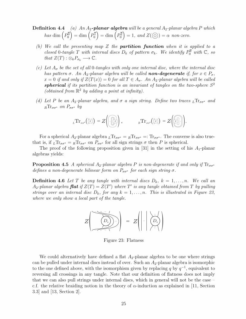
Definition 4.6 Let T be any tangle with internal discs Dk, k = 1, . . . , n. We call anA2-planar algebra flat if Z(T ) = Z(T ′) where T ′ is any tangle obtained from T by pullingstrings over an internal disc Dk, for any k = 1, . . . , n. This is illustrated in Figure 23,where we only show a local part of the tangle.

Figure 23: Flatness

We could alternatively have defined a flat A2-planar algebra to be one where stringscan be pulled under internal discs instead of over. Such an A2-planar algebra is isomorphicto the one defined above, with the isomorphism given by replacing q by q−1, equivalent toreversing all crossings in any tangle. Note that our definition of flatness does not implythat we can also pull strings under internal discs, which in general will not be the case –c.f. the relative braiding notion in the theory of α-induction as explained in [11, Section3.3] and [13, Section 2].

25

Figure 24: Flatness gives sphericity

Proposition 4.7 A flat A2-planar algebra is spherical.

Proof: Given a 0-tangle, we isotope the strings so that we have a σσ∗-tangle T , where|σ| = n for n ∈ N, with the n vertices along the top and bottom of T connected by closed

strings which pass to the left of T . Then the string from the nth vertex along the top andbottom of T can be pulled over all the other strings and all internal discs of T , introducingtwo opposite kinks, which contribute a scalar factor q8/3q−8/3 = 1 (see Figure 24). Wemay similarly pull the other strings which pass to the left of T over T . �

The A2-planar algebra PTL is clearly flat, since the labelling set L± = ∅. Then byProposition 4.7 we see that there is only one trace on the algebra VA2

m in Section 3.2.

4.4 The involution on P

We can define the adjoint T ∗ ∈ Pσ∗(L) of a tangle T ∈ Pσ(L) , where L has a ∗ operationdefined on it, by reflecting the whole tangle about the horizontal line that passes throughits centre and reversing all orientations. The labels xk ∈ L of T are replaced by labels x∗kin T ∗. If ϕ is the map which sends T → T ∗, then every region ϕ(R) of T ∗ has the samecolour as the region R of T . For any linear combination of tangles in Pσ(L) we extend ∗by conjugate linearity. Then P is an A2-planar ∗-algebra if each Pσ is a ∗-algebra, andfor a σ-tangle T with internal discs Dk with patterns σk, labelled by xk ∈ Pσk

, we have

Z(T )∗ = Z(T ∗),

where the labels of the discs in T ∗ are x∗k, and where the definition of Z(T )∗ is extended tolinear combinations of σ-tangles by conjugate linearity. For xj ∈ Pσj

, j = 1, 2, we definethe tangle m(x1, x2) ∈ Pσ1σ2 by:

.

Proposition 4.8 Let P be an A2-planar ∗-algebra. Then dim(Pσ) ≤ dim(Pσσ∗) for anysign string σ.

Proof: Fix an element y ∈ PTLσ∗ (i.e. the tangle y does not contain any internal discs)such that 0 6= cy = RTr(m(y, y∗)) ∈ C. We have an embedding ιy : Pσ → Pσσ∗ given by

26

Figure 25: Action of A ∈ Pσσ∗ on x ∈ Pσ

ιy( · ) = Z(m( · , y)). Let ι′y : Pσσ∗ → Pσ be the map defined by ι′y(A) = c−1y A(y∗), and

the action of Pσσ∗ on Pσ is given in Figure 25, for A ∈ Pσσ∗ , x ∈ Pσ. Then ι′y ◦ ιy = id on

Pσ, and thus dim(Pσ) ≤ dim(Pσσ∗).

Corollary 4.9 An A2-planar ∗-algebra P is finite dimensional if and only if dim(Pσσ∗) <∞ for any sign string σ.

The partition function Z : Pσ → C on an A2-planar algebra will be called positive if

RTrσ∗σ(m(x∗, x)) ≥ 0, for all x ∈ Pσ, and positive definite if RTrσ∗σ(m(x∗, x)) > 0, forall non-zero x ∈ Pσ. The proof of [31, Prop. 1.33] in the A1-case carries over to A2-planaralgebras where the only modification is that we allow possibly an odd number of verticeson discs, and different orientations on the strings.

Proposition 4.10 Let P be an A2-planar ∗-algebra with positive partition function Z.The following three conditions are equivalent: (i) P is non-degenerate, (ii) RTrσσ∗ ispositive definite, (iii) LTrσσ∗ is positive definite.

Then we have the following Corollary, c.f. [31, Cor. 1.36]:

Corollary 4.11 If P is a non-degenerate finite-dimensional A2-planar ∗-algebra with pos-itive partition function then Pσσ∗ is semisimple for all sign strings σ, so there is a uniquenorm on Pσσ∗ making it into a C∗-algebra. Each P σ is a Hilbert C∗-module over Pσσ∗ ,for the action of Pσσ∗ on Pσ given above.

Definition 4.12 We call an A2-planar algebra over R or C an A2-C∗-planar alge-

bra if it is a non-degenerate finite-dimensional A2-planar ∗-algebra with positive definitepartition function.

If P is a spherical A2-C∗-planar algebra we can define an inner-product on Pσ, for σ a

sign string of length n, by 〈x, y〉 = α−n/2Trσ∗σ(m(x∗, y)) for x, y ∈ Pσ. This inner productis normalized in the sense that 〈1σσ∗ , 1σσ∗〉 = 1 for any sign string σ.

5 A2-planar i, j-tangles

We will be particularly interested in the vector spaces Pσ for sign strings σ with a partic-ular form, since these will correspond exactly to the vector spaces in the double complexassociated to the SU(3)-subfactors. We describe these vector spaces in the next sections,and introduce certain basic tangles which will play an important role later.

27

An A2-planar i, j-tangle will be an A2-planar σ-tangle with external disc D = D0 andinternal discs D1, . . . , Dn, where each disc Dk, k ≥ 0, has pattern σ(k) = −jk · σ(k) · +jk ,where σ(k) is the alternating string of length 2ik which begins with ‘−’. We will positionthe vertices so that the first ik + jk are along the boundary for the upper half of the disc,which we will call the top edge, and the next ik + jk vertices are along the boundaryfor the bottom half of the disc, which we will call the bottom edge. We will use theconvention of numbering the vertices along the bottom edge in reverse order, so that the2(ik + jk)-th vertex is called the first vertex along the bottom edge. The total number ofsource vertices along the top edge is ⌊jk + (ik + 1)/2⌋, and the number of sink vertices is⌊ik/2⌋. For the outer boundary ∂D we impose the restriction b0 = 0.

It is important to note that what we here call an i, j-tangle is different from the (i, j)-tangles of Section 3. In both cases the integers i, j refer to the number of vertices alongthe top (and bottom) edge of the disc, however in an (i, j)-tangle the first i vertices areall sources, and the next j vertices are all sinks.

In the figures which follow we omit the orientation on the strings from the last ivertices along the top and bottom of an i, j-tangle – these will be alternating.

5.1 Some basic A2-planar i, j-tangles

The following basic tangles will be of importance to us:

• Inclusion tangles IRi,ji+1,j, IR

i,ji,j+1 and IR

i,j

i,j+1:

28

where the orientation of the rightmost string in IRi,ji+1,j is downwards for i even and

upwards for i odd. Both IRi,ji,j+1 and IR

i,j

i,j+1 add a new source vertex along the topimmediately to the right of the first j source vertices, and a sink vertex along the bottomimmediately to the right of the first j sink vertices along the bottom. These new verticesare regarded as being among the downwards oriented vertices rather than the alternating

vertices. They are connected by a through string, and IRi,ji,j+1, IR

i,j

i,j+1 differ only in that

the through string passes to the right of the inner disc in IRi,ji,j+1 and to the left in IR

i,j

i,j+1.

We have Z(IRi,ji+1,j) : Pi,j → Pi+1,j , and Z(IR

i,ji,j+1), Z(IR

i,j

i,j+1), : Pi,j → Pi,j+1.

For a flat A2-planar algebra, the two right inclusion tangles IRi,ji,j+1 and IR

i,j

i,j+1 are

equal, and we will simply write IRi,ji,j+1. For a spherical A2-planar algebra P , we define

tr(x) = α−i−j Tri,j(x) for x ∈ Pi,j. Then tr is compatible with the inclusions Pi,j ⊂ Pi,j+1

and Pi,j ⊂ Pi+1,j, given by IRi,ji,j+1, IR

i,ji+1,j respectively, and tr(1) = 1, and so defines a

trace on P itself. If P is a spherical A2-C∗-planar the inner-product defined at the end of

Section 4.4 is given on Pi,j by 〈x, y〉 = tr(x∗y) for x, y ∈ Pi,j, and is consistent with theinclusions Pi,j ⊂ Pi,j+1 and Pi,j ⊂ Pi+1,j given above, since tr is.

• Conditional expectation tangles ERi+1,ji,j and ERi,j+1

i,j :

(13)

The orientation of the string from vertex i+ j+1 on the inner disc of ERi+1,ji,j is clockwise

for i odd and anticlockwise for i even. We have Z(ERi+1,ji,j ) : Pi+1,j → Pi,j and Z(ER

i,j+1i,j ) :

Pi,j+1 → Pi,j.

Let P(1)i,j denote the subset of Pi,j spanned by all tangles where vertices j + 1 along

the top and bottom are connected by a through string which passes over every string itcrosses and such that there are no internal discs in the region between this string and theouter boundary of the tangle to the left of it. If P is a general A2-planar algebra withpresenting map Z, we define P

(1)i,j = Z(P

(1)i,j ) ⊂ Pi,j, and denote by P (1) ⊂ P the subspace

P (1) =⋃

i,j P(1)i,j . We also have left conditional expectation tangles ELi+1,j

i+1,j and ELi,j+1i,j+1:

29

where Z(ELi+1,ji+1,j) : Pi+1,j → P

(1)i+1,j.

The justification for calling the tangles in (13) conditional expectation tangles is seenin the following Lemma:

Lemma 5.1 Let P be an A2-C∗-planar algebra. For the tangles ERi+1,j

i,j and ERi,j+1i,j

defined in (13), E1(x) = Z(ERi+1,ji,j (x)) is the conditional expectation of x ∈ Pi+1,j onto

Pi,j with respect to the trace, and E2(y) = Z(ERi,j+1i,j (y)) is the conditional expectation of

y ∈ Pi,j+1 onto Pi,j with respect to the trace.

Proof: We first check positivity of E1(x) for positive x ∈ Pi+1,j . As P is an A2-C∗-

planar algebra, the inner-product defined above is positive definite. We need to showthat 〈E1(x)y, y〉 ≥ 0 for all y ∈ Pi,j. From Figure 26 we see that tr(y∗ERi+1,j

i,j (x)∗y) =

tr(y′∗x∗y′) = 〈xy′, y′〉 ≥ 0 for all y ∈ Pi,j, where y′ = ∈ Pi+1,j. From

we see that E1(axb) = aE1(x)b, for x ∈ Pi+1,j, a, b ∈ Pi,j. Since also 〈E1(x), y〉 = 〈x, y′〉,E1 is the trace-preserving conditional expectation from Pi+1,j onto Pi,j. The proof for E2

is similar. �

Similarly, Z(ELi+1,ji+1,j(x)) is the conditional expectation of x ∈ Pi+1,j onto P

(1)i+1,j .

Figure 26:

30

Figure 27: Maps ϕ : P2l+1,j+1(L) → P2l+2,j(L), ω : P2l,j+1(L) → P2l+1,j(L)

Figure 28: Maps ϕ−1 : P2l+2,j(L) → P2l+1,j+1(L), ω−1 : P2l+1,j(L) → P2l,j+1(L)

5.2 Dimensions in A2-planar algebras and PTL.

We now present some results regarding the dimensions of the different graded partsof A2-planar algebras. These will be needed later in Section 6. We define maps ϕ :P2l+1,j+1(L) → P2l+2,j(L), ω : P2l,j+1(L) → P2l+1,j(L) as in Figure 27 for x1 ∈ P2l+1,j+1(L),x2 ∈ P2l,j+1(L), where the white circle at the end of a string indicates that this vertex isnow regarded as one of the i vertices of Pi,j with alternating orientation (i = 2l+2, 2l+1for ϕ, ω respectively). The maps ϕ, ω are invertible, with ϕ−1, ω−1 as in Figure 28for x1 ∈ P2l+2,j(L), x2 ∈ P2l+1,j(L), where the solid black circle at the end of a stringindicates that this vertex is now regarded as one of the j + 1 vertices of Pi,j+1 with al-ternating orientation (i = 2l + 1, 2l for ϕ−1, ω−1 respectively). Clearly ϕ(P2l+1,j+1(L)) ⊂P2l+2,j(L). Since P2l+1,j+1(L) ⊃ ϕ−1(P2l+2,j(L)) then ϕ(P2l+1,j+1(L)) ⊃ P2l+2,j(L). Soϕ(P2l+1,j+1(L)) = P2l+2,j(L) and ϕ is a bijection. Similarly the map ω is a bijec-tion and ω(P2l,j+1(L)) = P2l+1,j(L). Let Z : Pi,j(L) → Pi,j be the presenting mapfor an A2-C

∗-planar algebra P . We define bijections ϕ : P2l+1,j+1(L) → P2l+2,j(L),ω : P2l,j+1(L) → P2l+1,j(L) by ϕ(x1) = Z(ϕ(x1)) and ω(x2) = Z(ω(x2)). Then

dim(Pi,j(L)) = dim(Pi+k,j−k(L)), (14)

dim(Pi,j) = dim(Pi+k,j−k), (15)

for all integers k such that −i ≤ k ≤ j. Note, (14) follows immediately from [44, Theorem6.3].

For L = ∅, we define PT Li,j to be the quotient of PTLi,j = Pi,j(∅) by the subspaceof zero-length vectors with respect to the inner-product on PTLi,j defined by 〈x, y〉 = x∗y,

for x, y ∈ PTLi,j, where T is the tangle defined as in Figure 11. The element ϕ(x) is

31

a zero-length vector in PTL2l+2,j if and only if x is a zero-length vector in PTL2l+1,j+1.Similarly, ω(x) is zero-length vector in PTL2l+1,j if and only if x is a zero-length vectorin PTL2l,j+1. Thus for all integers k with −i ≤ k ≤ j, dim(PT Li,j) = dim(PT Li+k,j−k).

6 A2-Planar algebra description of subfactors

We are now going to associate flat A2-planar C∗-algebras to the double sequences of

subfactors associated to ADE graphs with flat connections. These double sequences, in-troduced in [19], have a periodicity three coming from the A2-Temperley-Lieb algebra inthe horizontal direction, and a periodicity two coming from the subfactor basic construc-tion in the vertical direction. In Section 6.2 we give a diagrammatic form for the doublesequences for the Wenzl subfactors.

Let G be any finite SU(3) ADE graph with Coxeter number n. Let α = [3]q, q = eiπ/n,be the Perron-Frobenius eigenvalue of G and let (φv) be the corresponding eigenvector.Ocneanu [54] defined a cell system W on G by associating a complex number W

(△(αβγ)

),

called an Ocneanu cell, to each closed loop of length three △(αβγ) in G as in Figure 29,where α, β, γ are edges on G. These cells satisfy two properties, called Ocneanu’s type I,II equations respectively, which are obtained by evaluating the Kuperberg relations K2,K3 respectively, using the identification in Figure 29:

(i) for any type I frame in G we have

(16)

(ii) for any type II frame in G we have

(17)

The existence of these cells for the finite ADE graphs was shown in [21] with the exception

of the graph E(12)4 . Using these cells, we define a representation Uρ1,ρ2

ρ3,ρ4of the Hecke algebra

by

Uρ1,ρ2ρ3,ρ4

=∑

λ

φ−1s(ρ1)

φ−1r(ρ2)

W (△(λ,ρ3,ρ4))W (△(λ,ρ1,ρ2)), (18)

for edges ρ1, ρ2, ρ3, ρ4, λ of G.

32

Figure 29: Cells associated to trivalent vertices

As in [19], with any choice of distinguished vertex ∗, we define the double sequence(Bi,j) of finite dimensional algebras by:

B0,0 ⊂ B0,1 ⊂ B0,2 ⊂ · · · −→ B0,∞

∩ ∩ ∩ ∩B1,0 ⊂ B1,1 ⊂ B1,2 ⊂ · · · −→ B1,∞

∩ ∩ ∩ ∩B2,0 ⊂ B2,1 ⊂ B2,2 ⊂ · · · −→ B2,∞

∩ ∩ ∩ ∩...

......

...

The Bratteli diagrams for horizontal inclusions Bi,j ⊂ Bi,j+1 are given by G. If G is three-colourable, the vertical inclusions Bi,j ⊂ Bi+1,j are given by its j, j + 1-part Gj,j+1, wherep = τ(p) is the colour of p for p = j, j + 1. We identify B0,0 = C with the distinguishedvertex ∗ of G.

Then for the inclusionsBi,j ⊂ Bi,j+1

∩ ∩Bi+1,j ⊂ Bi+1,j+1

(19)

with i even, we define a connection by

Xρ1,ρ2ρ3,ρ4

=

ρ1−→

ρ3↓ ↓ρ2−→ρ4

= q2/3δρ1,ρ3δρ2,ρ4 − q−1/3 Uρ1,ρ2ρ3,ρ4

, (20)

We denote by G the reverse graph of G, which is the graph obtained by reversing thedirection of every edge of G. For the inclusions (19) with i odd, let ρ1, ρ4 be edges on G

and let ρ2, ρ3 be edges on the reverse graph G (so that ρ2, ρ3 are edges on G). We definethe connection by

Xρ1,ρ2ρ3,ρ4

=

ρ1−→

ρ3↓ ↓ρ2−→ρ4

=

√φs(ρ3)φr(ρ2)

φr(ρ3)φs(ρ2)

ρ4−→

ρ3↓ ↓ρ2−→ρ1

. (21)

It was shown in [21] that these connections satisfy the unitarity axiom

∑

ρ3,ρ4

Xρ1,ρ2ρ3,ρ4

Xρ′1,ρ

′2

ρ3,ρ4 = δρ1,ρ′1δρ2,ρ′2. (22)

Then for the inclusions (19) an element indexed by paths in the basis ❄✲ can betransformed to an element indexed by paths in the basis

✲

❄using the above connections:

33

Let (σ · σ′ · α1 · α2, σ · σ′ · α′1 · α

′2) be an element in Bi+1,j+1 in the basis ❄✲ , where σ is

a horizontal path of length j, σ′ is a vertical path of length i, α1, α′1 are vertical paths of

length 1, α2, α′2 are horizontal paths of length 1, and r(α2) = r(α′

2). We transform thisto an element in the basis

✲

❄by

(σ · σ′ · α1 · α2, σ · σ′ · α′1 · α

′2) =

∑

βi,β′i

β1−→

α1↓ ↓β2

−→α2

β′1−→

α′1↓ ↓β′

2−→α′2

(σ · σ′ · β1 · β2, σ · σ′ · β ′

1 · β′2),

where the summation is over all horizontal paths β1, β′1 of length 1, and vertical paths β2,

β ′2 of length 1.The Markov trace on Bi,j is defined as in [19] by

tr((σ1, σ2)) = δσ1,σ2[3]−kφr(σ1), (23)

for (σ1, σ2) ∈ Bi,j , where k = i+j. We define Bi,∞ to be the GNS-completion of⋃

k≥0Bi,k

with respect to the trace. As in [19], the braid elements

appear as the connection.If G is three-colourable then its adjacency matrix ∆G which may be written in the

form

∆G =

0 ∆01 00 0 ∆12

∆20 0 0

,

where ∆01, ∆12 and ∆20 are matrices which give the number of edges between each 0,1,2-coloured vertex respectively of G to each 1,2,0-coloured vertex respectively. By a suitableordering of the vertices the matrix ∆12 may be chosen to be symmetric. These matricessatisfy the conditions

∆T01∆01 = ∆20∆

T20 = ∆2

12, ∆01∆T01 = ∆T

20∆20, (24)

which follow from the fact that ∆G is normal [22].

Lemma 6.1 For the double sequence (Bi,j) defined above, dim(Bi,j) = dim(Bi+k,j−k) forall integers k such that −i ≤ k ≤ j.

Proof: If G is not three-colourable, then Bi,j is the space of all pairs of paths of lengthi + j on G, hence the result is trivial. For the three-colourable graphs, let Λ1

i,j be theproduct of j matrices Λ1

i,j = ∆01∆12∆20∆01 · · ·∆j−1,j, and Λ2i,j the product of i matrices

Λ2i,j = ∆j,j+1∆

Tj,j+1

∆j,j+1∆Tj,j+1

· · ·∆′, where ∆′ is ∆j,j+1 if i is odd, ∆Tj,j+1

if i is even, and

p is the colour of p. Then if Λi,j = Λ1i,jΛ

2i,j, the dimension of Bi,j is given by

(Λi,jΛ

Ti,j

)0,0.

Using (24) it is easy to show by induction that Λi,jΛTi,j = (∆01∆

T01)

i+j . So dim(Bi+k,j−k) =(Λi+k,j−kΛ

Ti+k,j−k

)0,0

=((∆01∆

T01)

i+j)0,0

= dim(Bi,j). �

34

For all i, j ≥ 0 we define operators U−k ∈ Bi,j, k = 0, 1, . . . , j − 1, which satisfy theHecke relations H1-H3, by

U−k =∑

|ζ1|=j−2−k,|ζ′|=i

|γi|=|ηi|=1,|ζ2|=k

Uγ2,η2γ1,η1

(ζ1 · γ1 · η1 · ζ2 · ζ′, ζ1 · γ2 · η2 · ζ2 · ζ

′), 0 ≤ k ≤ j − 2,

U−j+1 =∑

|ζ|=j−1,|ζ′|=i−1

|γi|=|η′i|=1

Uγ2,η2γ1,η1

(ζ · γ1 · η′1 · ζ

′, ζ · γ2 · η′2 · ζ

′),

where ξ, ξ′ are horizontal, vertical paths respectively, and Uγ2,η2γ1,η1 are the Boltzmann weights

for A(n). The embedding of U−k ∈ Bi,j into Bi+1,j is U−k, whilst the embedding ofU−k ∈ Bi,j into Bi,j+1 is U−k−1. We have Bi,j ⊃ alg(U−j+1, U−j+2, . . . , U−1, U0). WhenG = A(n), the algebra Bl,j = alg(U−j+1, U−j+2, . . . , U−l) for l = 0, 1 [19].

Lemma 6.2 The square (19) is a commuting square.

Proof: Note that for the A graphs, the result follows by [70, Prop. 3.2]. However, weprove the case for a general SU(3) ADE graph G. By [20, Theorem 11.2], the square (19)is a commuting square if and only if the corresponding connection satisfies

∑

σ2,σ4

φr(σ2)

√φs(σ3)φs(σ′

3)

φs(σ2)φs(σ4)

σ1−→σ3↓ ↓σ2

−→σ4

σ′1−→

σ′3↓ ↓σ2

−→σ4

= δσ1,σ′1δσ3,σ′

3, (25)

where σ1, σ′1 are any edges on the graph of the Bratteli diagram for Bi,j ⊂ Bi,j+1, σ3,

σ′3 are any edges on the graph of the Bratteli diagram for Bi,j ⊂ Bi+1,j , σ2 is any edge

on the graph of the Bratteli diagram for Bi,j+1 ⊂ Bi+1,j+1, and σ4 is any edge on thegraph of the Bratteli diagram for Bi+1,j ⊂ Bi+1,j+1, such that s(σ2) = r(σ1) = r(σ′

1) ands(σ4) = r(σ3) = r(σ′

3). Equation (25) is easily verified for both connections (20), (21)using equations (16) and (17) and the fact that [3] is the Perron-Frobenius eigenvaluefor G. This computation is essentially the algebraic verification of the first diagrammaticrelation given in (8). �

Then as in [19], we define the Jones projections in Bi,j , for i = 1, 2, . . ., by:

ei−1 =∑

|ζ|=j,|ζ′|=i−2

|γ′|=|η′|=1

1

[3]

√φr(γ′)φr(η′)

φr(ζ′)(ζ · ζ ′ · γ′ · γ′, ζ · ζ ′ · η′ · η′) (26)

where ξ denotes the reverse edge of ξ. Let EMi−1be the conditional expectation from

Bi+1,∞ onto Bi,∞ with respect to the trace. For x ∈ Bi+1,j, EMi−1(x) is given by the

conditional expectation of x onto Bi,j, because of Lemma 6.2. Clearly elx = xel, forx ∈ Bl−1,∞, since x and el live on distinct parts of the Bratteli diagram. It can be shownthat elxel = EMl−1

(x)el for all x ∈ Bl,∞, and that Bl+1,∞ is generated by Bl,∞ and el. Thenel is the Jones projection for the basic construction Bl−1,∞ ⊂ Bl,∞ ⊂ Bl+1,∞, l = 1, 2, . . . .By [59, Prop. 1.2] if we set N = B0,∞ and M = B1,∞, the sequence B0,∞ ⊂ B1,∞ ⊂B2,∞ ⊂ B3,∞ ⊂ · · · can be identified with the Jones tower N ⊂ M ⊂ M1 ⊂ M2 ⊂ · · ·. Itwas shown in [19] that for G = A(n), n < ∞, if ∗ is now the apex vertex (0, 0) of A(n),then this subfactor is the same as Wenzl’s subfactor in [70] for SU(3), and we have thefollowing theorem from [19] (Theorems 3.3, 5.8 and Corollary 3.4):

35

Theorem 6.3 In the double sequence (Bi,j) above for G = A(n) or D(n), n <∞, with ∗ thevertex with lowest Perron-Frobenius weight, we have B′

0,∞∩Bi,∞ = Bi,0, i.e. N′∩Mi−1 =

Bi,0. The principal graph for the above subfactors is given by the 01-part G01 of G.

The connection will be called flat [51, 52] if any two elements x ∈ Bk,0 and y ∈ B0,l

commute. This is equivalent to the relation

(27)

for any paths σ, ρ on the graphs G and G.Then for graphs where the connection (20) is flat, the higher relative commutants are

given by the Bk,0, that is, B′0,∞ ∩ Bk,∞ = Bk,0, by Ocneanu’s compactness argument [52]

in the setting of our SU(3) subfactors. If G is a graph with flat connection, then theprincipal graph of the subfactor B0,∞ ⊂ B1,∞ will be the 01-part G01 of G.

Flatness of the connection for the A, D graphs was shown in Theorem 6.3, wherethe distinguished vertex ∗ was chosen to be the vertex with lowest Perron-Frobeniusweight. The flatness of the connection for the exceptional E graphs in not decided here.The determination of whether the connection is flat in these cases is a finite problem,involving checking the identity (27) for diagrams of size 2dG01 × 2(dG + 3), where dG isthe depth of G and dG01 is the depth of its 01-part G01. This is because for the verticalpaths, the algebras Bl+1,j are generated by Bl,j and the Jones projection el for all l ≥ dG01,and el does not change its form under the change of basis using the connection. For thehorizontal paths, by [22, Lemma 4.7] we see that the algebras Bi,l+1 are generated by Bi,l

and U−l for l ≥ dG + 3, and the Hecke operators U−l do not change their form under thechange of basis, as is shown in the proof of Theorem 6.4 below.

We have not yet been able to determine whether or not the connection defined by(20), (21) is flat for the E cases, where the vertex ∗ is chosen to be the vertex with lowestPerron-Frobenius weight, since the number of computations involved, though finite, isextremely large. We expect that this connection will be flat for the exceptional graphsE (8), E

(12)1 and E (24), since these graphs appear as the M-N graphs for type I inclusions

N ⊂ M . We expect that this connection will not be flat for the remaining exceptionalgraphs E

(12)2 , E

(12)4 and E

(12)5 for any choice of distinguished vertex ∗. We also expect that

the connection will not be flat for the A∗, D∗ graphs, for any choice of distinguished vertex∗. The principal graph for the graphs with a non-flat connection is given by its flat part,which should be the type I parents given in [22].

6.1 Flat A2-C∗-planar algebra from SU(3) ADE subfactors

We will now associate a flat A2-C∗-planar algebra P to a double sequence (Bi,j) of finite

dimensional algebras with a flat connection.We define the tanglesW−k, k = 0, . . . , j−1, and fl, l = 1, . . . , i, in Pi,j(∅) as in Figure

30, where the orientations of the strings without arrows depends on the parity of i and l.

36

Figure 30: Tangles W−k and fl

Let G denote the graph G with all orientations reversed and let Pσ be the space ofclosed paths on G, G which start at the distinguished vertex ∗, where a ‘−’ denotes thatan edge is on G and ‘+’ denotes that an edge is on G. We will define a presenting mapZ : Pσ(P ) → Pσ such that Pi,j

∼= Bi,j , where we identify a path γ1 ·γ2 of length 2m in Pi,j

with the pair of paths (γ1, γ2) of length m (i.e. an element in Bi,j) by cutting the originalpath in half and reversing the path γ2. We define a ∗-operation on P by γ∗ = γ ∈ Pσ∗ forγ ∈ Pσ. For γ1 · γ2 ∈ Pi,j, (γ1 · γ2)

∗ = γ2 · γ1 which is mapped to (γ2, γ1) ∈ Bi,j under theisomorphism Pi,j

∼= Bi,j . Note that (γ2, γ1) = (γ1, γ2)∗ in Bi,j, so the ∗-structure on B is

preserved under the isomorphism.Let T be a labelled tangle in Pσ with m internal discs Dk with pattern σk and labels

xk ∈ Pσk, k = 1, . . . , m. We define Z(T ) as follows. First, convert all the discs Dk to

rectangles (including the outer disc) so that its edges are parallel to the x, y-axes, and suchthat all the vertices on its boundary lie along the top edge of the rectangle. Next, isotopethe strings of T so that each horizontal strip only contains one of the following elements:a rectangle with label xk, a cup, a cap, a Y-fork, or an inverted Y-fork (see Figures 31, 32and 33). For a tangle T ∈ Pσ with l horizontal strips sl, where s1 is the highest strip, s2the strip immediately below it, and so on, we define Z(T ) = Z(s1)Z(s2) · · ·Z(sl), which

will be an element of Pσ. We then define Z(T ) by Z(T ) = Z(T ) if γ is a path of odd

length, and Z(T ) =√φs(γ1)/

√φr(γk)Z(T ) if γ = γ1 · γ2 · · · γ2k is a path of length 2k,

where the γi are edges on G or G. Note that we have P 0σ = P 1

σ = P 2σ . This algebra is

normalized in the sense that for the empty tangle ©, Z(©) = 1. We will need to showthat this definition only depends on T , and not on the decomposition of T into horizontalstrips.

Figure 31: Cup ∪(i) and cap ∩(i)

Figure 32: Y-forks g(i) and g(i)

37

Figure 33: Inverted Y-forks f(i) and f(i)

Let C be the set of all strips containing one of these elements except for a labelledrectangle. We will use the following notation for elements of C, as shown in Figures 31,32 and 33: A strip containing a cup, cap will be ∪(i), ∩(i) respectively, where there arei− 1 vertical strings to the left of the cup or cap. A strip containing an incoming Y-fork,inverted Y-fork will be g(i), f(i) respectively, where there are i− 1 vertical strings to theleft of the (inverted) Y-fork. A bar will denote that it is an outgoing (inverted) Y-fork.

For an element c ∈ C we have sign strings σ1, σ2 given by the endpoints of thestrings along the top, bottom edge respectively of the strip (we will call these endpointsvertices), where, along the top edge ‘+’ is given by a sink and ‘−’ by a source, and alongthe bottom edge ‘+’ is given by a source and ‘−’ by a sink. The leftmost region of thestrip c corresponds to the vertex ∗ of G, and each vertex along the top (or bottom) with

downwards, upwards orientation respectively, corresponds to an edge on G, G respectively.Then the top, bottom edge of the strip is labelled by elements in Pσ1 , Pσ2 respectively,which start at ∗. Then Z(c) defines an operator Mc ∈ End(Pσ2 , Pσ1) as follows.

For a cup ∪(i), and paths α = α1 · α2 · · ·αj, β = β1 · · ·βj+2,

(M∪(i))α,β = δα1,β1δα2,β2 · · · δαi−1,βi−1δαi,βi+2

δαi+1,βi+3· · · δαm,βm+2δβi,βi+1

√φr(βi)√φs(βi)

. (28)

For a cap ∩(i),M∩(i) =M∗

∪(i) . (29)

For an incoming (inverted) Y-fork g(i) or f(i),

(Mg(i))α,β = δα1,β1 · · · δαi−1,βi−1δαi+1,βi+2

· · · δαm,βm+1

1√φs(αi)φr(αi)

W (△(αi,βi,βi+1)),

(30)

(Mf(i))α,β = δα1,β1 · · · δαi−1,βi−1δαi+2,βi+1

· · · δαm+1,βm

1√φs(βi)φr(βi)

W (△(βi,αi+1,αi)),

(31)

where W is a cell system on G satisfying (16) and (17).

For an outgoing (inverted) Y-fork g(i) or f(i),

Mg

(i) = M∗f(i), (32)

Mf

(i) = M∗g(i). (33)

For a strip b containing a rectangle with label x = γ, where γ is a single path in Pσ,we define the operator Mb = Z(b) as follows. Let p, p′ be the number of vertical strings

38

Figure 34: Z(b) for horizontal strip b containing a rectangle

to the left, right respectively of the rectangle in strip b, with orientations given by thesign strings σ(p), σ(p′) respectively. We attach trivial tails µ of length p to x, where µ hasedges on G, G as dictated by the sign string σ(p), so that we have a sum

∑µ γ ·µ of paths

in the basis given by the sign string σσ(p). We use the connection to transform this to alinear combination of paths in the basis given by the sign string σ(p)σ. By flatness of theconnection on G, this will be an element of the form

∑ζ,µ pζµ · ζ , where pζ ∈ C are given

by the connection, ζ are paths in Pσ, and µ are again paths in Pσ(p) . We then add trivialtails ν of length p′ to this element, where ν has edges on G, G as dictated by the signstring σ(p′). This gives an element

∑ζ,µ,ν pζµ ·ζ ·ν, which is an element in Pσ(p)σσ(p′) . Then

we define Z(b) ∈ End(Pσ(p)σ(p′), Pσ(p)σσ(p′)) to be∑

ζ,µ,ν pζ(µ · ζ · ν, µ · ν). We extend thisdefinition of Z(b) linearly to strips b where the label x is a linear combination of paths inPσ. This definition means that Z(b) is defined as the product Z(s1)Z(s2), where s1, s2are the horizontal strips on the right hand side of Figure 34. Thus we see that P is a flatA2-planar algebra.

The following theorem shows that for anADE graph with a flat connection, P =⋃

σ Pσ

is a flat A2-C∗-planar algebra, such that the subalgebra

⋃i,j Pi,j is given by the subfactor

double complex (Bi,j).

Theorem 6.4 Let G be an ADE graph such that the connections (20), (21) are flat. Theabove definition of Z(T ) for any A2-planar tangle T makes P =

⋃σ Pσ into a flat A2-C

∗-

planar algebra, such that Pi,j∼= Bi,j, with dim

(P 00

)= dim

(P 10

)= dim

(P 20

)= 1. This

A2-C∗-planar algebra has parameter α = [3] (the Perron-Frobenius eigenvalue for G), and

Z(Iσσ∗(x)) = x, where Iσσ∗(x) is the tangle Iσσ∗ with x ∈ Pσσ∗ as the insertion in itsinner disc. For x ∈ Pi,j, i, j ≥ 0, we have(i) Z(W−k) = U−k, k ≥ 0,(ii) Z(fl) = αel, l ≥ 1,

(iii)

(iv)

(v)

39

In the first equation of (iii) the first j+1 vertices along the top and bottom of the rectan-gle are joined by loops, and the second equation only holds for i 6= 0. In the first, secondequation of (iv) respectively, the x on the right hand side is considered as an element ofPi+1,j, Pi,j+1 respectively.

Proof: First we show that Z(T ) does not change if the labelled tangle is changed by iso-

topy of the strings. We use the following notation ∂αi+k ,βj+k

αi,βj:= δαi,βj

δαi+1,βj+1· · · δαi+k ,βj+k

.The identities are simply a consequence of the identification in Figure 29 of the Ocneanucells with trivalent vertices, and of cups and caps with the Perron-Frobenius weights.

Case (1)- Topological moves: We consider the cup-cap simplifications (which Kauffmancalls Move Zero in [38]) shown in Figure 35. For the first cup-cap simplification of Figure35 we have

(M∪(i+1)M∩(i))α,β =∑

γ

(M∪(i+1))α,γ (M∪(i))β,γ

=∑

γ

∂αi,γiα1,γ1

∂αm,γm+2αi+1,γi+3

δγi+1,γi+2

√φr(γi+1)√φs(γi+1)

∂βi−1,γi−1

β1,γ1∂βm,γm+2

βi,γi+2δγi,γi+1

√φr(γi)√φs(γi)

= δα,β. (34)

The second simplification in Figure 35 follows from the first, since

M∪(i)M∩(i+1) = (M∪(i+1)M∩(i))T = 1. (35)

Case (2)- Isotopies involving incoming trivalent vertices: We require the identities of Fig-ure 36. For (a) we verify that (Mg(i)M∩(i+1))α,β = (Mf(i))α,β, and similarly for the identi-ties (b), (c) and (d). For (e) we need to verify that (M∪(i−1)Mg(i))α,β = (M∪(i−1)Mg(i−1))α,β.The corresponding identities for outgoing trivalent vertices hold in the same way. Thenthe identity in Figure 37 follows from the cup-cap simplifications and identities (a)-(e) forincoming and outgoing trivalent vertices.

Kuperberg relations: Before checking isotopies that involve rectangles, we will show thatthe Kuperberg relations K1-K3 are satisfied. For K1, a closed loop gives

(M∪(i)M∩(i))α,β =∑

γ

(M∪(i))α,γ (M∪(i))β,γ = δα,β∑

γi:s(γi)=r(αi−1)

φr(γi)

φs(γi)

= δα,β[3], (36)

Figure 35: Two cup-cap simplifications

40

Figure 36: Isotopies involving an incoming trivalent vertex

Figure 37: An isotopy involving an incoming and outgoing trivalent vertex

by the Perron-Frobenius eigenvalue equation Λx = [3]x, where x = (φv)v, and Λ is ∆G or∆T

G depending on whether the loop has anticlockwise, clockwise orientation respectively.Relations K2 and K3 are essentially Ocneanu’s type I, II formulas (16), (17) respectively.

Property (ii) and the connection: We obtain

Z(W−k) =∑

|ζ1|=j−2−k,|ζ′|=i

|γi|=|ηi|=1,|ζ2|=k

Uγ2,η2γ1,η1

ζ1 · γ1 · η1 · ζ2 · ζ′ · ζ ′ · ζ2 · η2 · γ2 · ζ1,

and we identify the path ζ1 · γ1 · η1 · ζ2 · ζ′ · ζ ′ · ζ2 · η2 · γ2 · ζ1 ∈ Pσσ∗ with the matrix unit

(ζ1 · γ1 · η1 · ζ2 · ζ′, ζ1 · γ2 · η2 · ζ2 · ζ

′) ∈ End(Pσ, Pσ). The property (ii) in the statement ofthe theorem follows from (18) and the definition of U−k. Since U−k is given by the tangleW−k, we see that the partial braiding defined in (7) gives the connection, where (20) is

given by and (21) is given by . For the latter connection, which involves the reverse

41

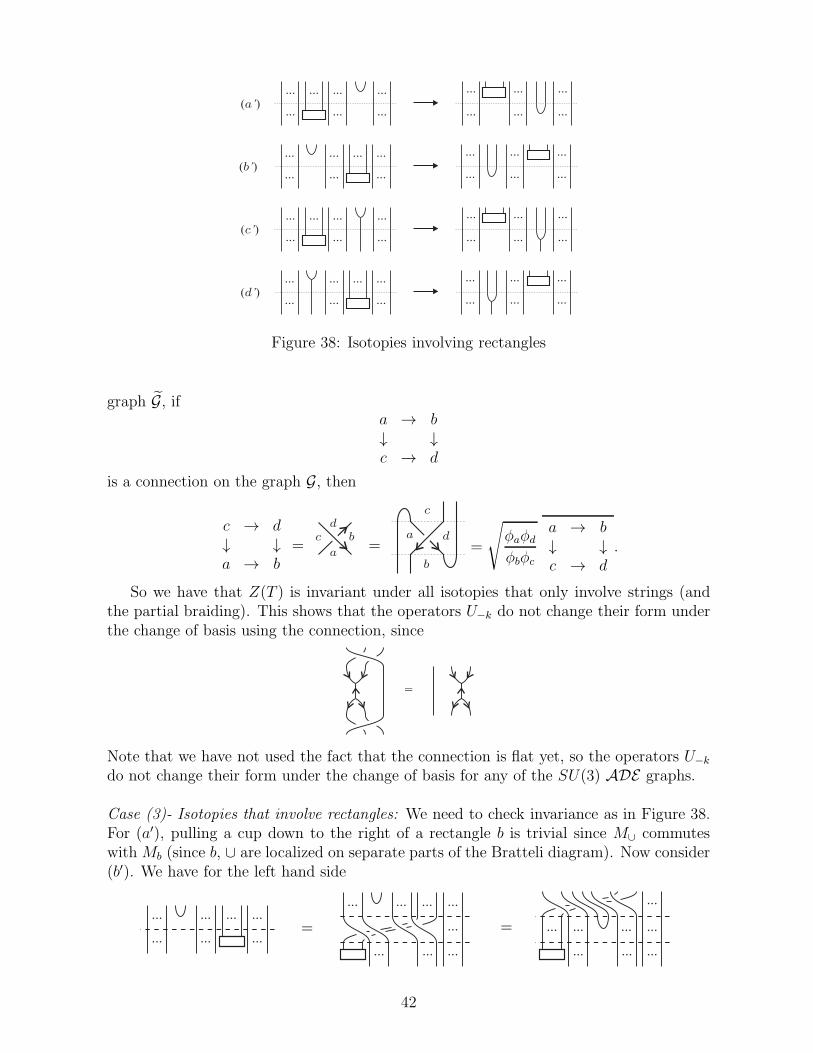
Figure 38: Isotopies involving rectangles

graph G, ifa → b↓ ↓c → d

is a connection on the graph G, then

c → d↓ ↓a → b

= = =

√φaφd

φbφc

a → b↓ ↓c → d

.

So we have that Z(T ) is invariant under all isotopies that only involve strings (andthe partial braiding). This shows that the operators U−k do not change their form underthe change of basis using the connection, since

Note that we have not used the fact that the connection is flat yet, so the operators U−k

do not change their form under the change of basis for any of the SU(3) ADE graphs.

Case (3)- Isotopies that involve rectangles: We need to check invariance as in Figure 38.For (a′), pulling a cup down to the right of a rectangle b is trivial since M∪ commuteswithMb (since b, ∪ are localized on separate parts of the Bratteli diagram). Now consider(b′). We have for the left hand side

42

Figure 39: An isotopy involving two rectangles

Figure 40: Rotation of internal rectangles by 2π

where the first equality is the definition of Z(s) for a horizontal strip s containing arectangle b with through strings on its left, and the second equality follows since Z isinvariant under all isotopies that only involve strings and the partial braiding. Similarly,for the right hand side we obtain

and the result follows from (a′). The situations for (c′), (d′) are similar to (a′), (b′). Wealso have the isotopy in Figure 39. Let x ∈ Pσ1 , y ∈ Pσ2 be given by the paths α1,α2 respectively, of lengths k2, k4 respectively. The case for general elements x ∈ Pσ1 ,y ∈ Pσ2 follows by linearity. Consider first the case where k1 = k3 = k5 = 0. ThenZ(s1)Z(s2) = (α1 · α2, ∗) ∈ End(P0, Pσ1σ2). For the right-hand side we have Z(s4) =(α1, ∗) ∈ End(P0, Pσ1) and Z(s3) =

∑µ,α′

2pα′

2(µ · α′

2, µ) ∈ End(Pσ1 , Pσ1σ2), where pα′2∈ C

are given by the connection. By the flatness condition (27), pα′2= δα′

2,α2, so we have

Z(s3)Z(s4) =∑

µ(µ · α2, µ)(α1, ∗) = (α1 · α2, ∗) = Z(s1)Z(s2). The cases where k1, k3, k5are non-zero follow similarly.

Case (4)- Rotational invariance: The other isotopy that needs to be checked is the rotationof internal rectangles by 2π. We illustrate the case where rectangle b has kb = 2 verticesalong its top edge in Figure 40. We have divided ρ(x) into horizontal strips s1, . . . , s5.

Let x ∈ Pσbbe the label of the rectangle b, where x is the single path γ of length kb.

The strip s3 containing the rectangle b gives Y = Z(s3) =∑

µ,ζ,ν pζ(µ · ζ · ν, µ · ν), wherepζ ∈ C are given by the connection, and µ, ν are paths of length kb with edges on the

graphs G or G as dictated by the sign strings σ∗b , σb respectively.

For a horizontal strip s1 and strip s2 immediately below it, an entry in the operatorZ(s′) = Z(s1)Z(s2) is only defined when the path corresponding to the bottom edge ofthe strip s1 is equal to the path given by the top edge of s2. So for example, for the two

43

Figure 41: Horizontal strips s1, s2

strips s1, s2 in Figure 41, even though there are non-zero entries in Z(s2) for any pathα = α1 · α2 · · ·, the entries in Z(s′) will be zero unless edge αi is the reverse edge αi+1 ofαi+1 since the entries in Z(s2) are only non-zero for the paths γ = γ1 · γ2 · · · such thatγi = γi+1.

Let ε = ε1 ·ε2 · · · ε3kb, ε′ = ε′1 ·ε

′2 · · · ε

′kb·ε′2kb ·ε

′2kb+1 · · · ε

′3kb

be two paths which label theindices for Y . For simplicity we consider the case kb = 2 as in Figure 40. By consideringthe horizontal strip s3 containing the rectangle, we see that Yε,ε′ = 0 unless εi = ε′i fori = 1, 2, 5, 6. We see that in ρ(x), ε1 is the same string as ε4 and ε6, but that ε4 has

the opposite orientation to ε1 and ε6. We define the operator Y by Yε,ε′ = 0 unless

ε1 = ε4 = ε6 and ε2 = ε3 = ε5, and Yε,ε′ = Yε,ε′ otherwise. Then

ρ(x) = M∪(1)M∪(2) · · ·M∪(kb)YM∩(kb)M∩(kb−1) · · ·M∩(1)

= M∪(1)M∪(2) · · ·M∪(kb) Y M∩(kb)M∩(kb−1) · · ·M∩(1) .

For any two paths ε and ε′ such that Yε,ε′ is non-zero, the caps contribute a scalar factor√φr(ε2)/

√φs(ε1) =

√φs(ε1)/

√φs(ε1) = 1, and similarly we have a scalar factor of 1 from

the cups. Now ε1 is an edge on G (or G) with s(ε1) = ∗, and hence ρ(x) is only non-zerofor paths ε3 · ε4 such that s(ε3) = ∗. By the flatness of the connection on G, the onlypath ζ starting from ∗ for which pζ 6= 0 is γ, i.e. the original element x. Then theresulting operator given by ρ(x) will have all entries 0 except for that for γ, and we haveρ(x) = γ = x.

Then Z(T ) is invariant under all isotopies of the tangle T .

Properties (i)-(v): Property (i) follows from the definition of ei in (26), and property (ii)has already been shown. Now consider property (iii). We start with the first equation.For any x ∈ Pi,j, the left hand side is equal to Z(ELi,0

i,0ERi,1i,0ER

i,2i,1 · · ·ER

i,ji,j−1(x)), and

so gives is the conditional expectation of x onto P(1)i,0 (see Section 5.1). We now show

that P(1)i,0 = M ′ ∩Mi−1. Embedding the subalgebra P

(1)i,0 ⊂ Pi,0 in Pi,∞ we see that it

lives on the last i− 1 strings, with the rest all vertical through strings. Then P(1)i,0 clearly

commutes with M , since the embedding of M = P1,∞ in Pi,∞ has the last i − 1 strings

all vertical through strings, so we have M ′ ∩Mi−1 ⊃ P(1)i,0 . For the opposite inclusion, we

extend the double sequence (Bi,j) to the left to get

44

B0,0 ⊂ B0,1 ⊂ B0,2 ⊂ · · · −→ B0,∞

∩ ∩ ∩ ∩B1,−1 ⊂ B1,0 ⊂ B1,1 ⊂ B1,2 ⊂ · · · −→ B1,∞

∩ ∩ ∩ ∩ ∩B2,−1 ⊂ B2,0 ⊂ B2,1 ⊂ B2,2 ⊂ · · · −→ B2,∞

∩ ∩ ∩ ∩ ∩...

......

......

Note that B1,−1 = B0,0 = C. Since the connection is flat, by Ocneanu’s compactnessargument [52] we have B′

1,∞ ∩Bi,∞ = Bi,−1. Let x = (α1, α2) be an element of Bi,−1. Weembed x in Bi,0 by adding trivial horizontal tails of length one, and using the connectionwe can write x as x′ =

∑µ pβ1,β2(µ·β1, µ·β2), where pβ1,β2 ∈ C. We see that x′ ∈ Bi,0 = Pi,0

is summed over all trivial edges µ of length 1 starting at ∗, and hence is given by Z(T )for some T ∈ Pi,0 which has a vertical through string from the first vertex along the top

to the first vertex along the bottom, i.e x ∈ P(1)i,0 . So M

′ ∩Mi−1 = Bi,−1 ⊂ P(1)i,0 .

For the second equation of (iii), if x ∈ Pi,∞ then x→ Z(Ei,∞i−1,∞(x)) is the conditional

expectation onto Pi−1,∞ =Mi−2, and the result for x ∈ Pi,j follows by Lemma 6.2.Property (iv) is clear. Finally, for (v) let x be an element (α, β), where α, β are paths

of length k on G. Then

[3]−kZ(x) = [3]−kδα,βφr(α)

φ∗φ2∗ = [3]−kδα,βφr(α) = tr((α, β)),

since φ∗ = 1, where x is the tangle defined by joining the last vertex along the top of T tothe last vertex along the bottom by a string which passes round the tangle on the righthand side, and joining the other vertices along the top to those on the bottom similarly.

To see the ∗-structure, note that under ∗ the order of the strips is reversed so that(Z(s1)Z(s2) · · ·Z(sl))

∗ = Z(sl)∗Z(sl−1)

∗ · · ·Z(s1)∗. For a strip containing a rectangle

with label x ∈ Pσ given by a path γ, ∗ sends the rectangle to the right hand side ofFigure 42. Since s(γ) = r(γ), the caps contribute a coefficient

√φr(γ)/

√φs(γ) = 1 as

required. For M∪(i) , the ratio√φr(βi)/

√φs(βi) does not change under reflection of the

tangle and reversing the orientation, so that (M∪(i))∗ is the conjugate transpose of M∪(i)

as required, and similarly for M∩(i) . Since the involution of the strip g(i) containing an

incoming trivalent vertex is f(i), whilst the involution of the strip f

(i) containing anincoming trivalent vertex is g(i), by (32), (M

g(i))∗ is the conjugate transpose of Mf(i) and

by (33), (Mf

(i))∗ is the conjugate transpose of Mg(i) as required. To show that P is anA2-C

∗-planar algebra we need to show that P is non-degenerate, which is immediate fromproperty (v) in the statement of the theorem, Proposition 4.10 and the fact that tr ispositive definite. �

Figure 42: The ∗-structure on strips containing rectangles

45

Definition 6.5 We will say that an A2-planar algebra P is an A2-planar algebra for thesubfactor N ⊂ M if P0,∞ = N , P1,∞ = M , Pn,∞ = Mn−1, the sequence P0,0 ⊂ P1,0 ⊂P2,0 ⊂ · · · is the tower of relative commutants, and if conditions (i)-(v) of Theorem 6.4are satisfied.

Suppose P is the A2-planar algebra given by the double complex (Bi,j) for an SU(3)ADE subfactor N ⊂ M . Then the A2-planar subalgebra P (1) ⊂ P is the A2-planaralgebra given by the double complex for the subfactor M ⊂ M1.

For the subalgebra Q introduced in §4.1, we give an alternative proof of Jones’ theoremthat extremal subfactors give planar algebras [31, Theorem 4.2.1] in the finite depthcase. Jones’ proof uses the bimodule setup- he works with the von Neumann algebrasthemselves, identifying the relative commutants with tensor powers of the von Neumannalgebra M . The rotation tangle ρ plays an important role in his proof of Theorem 4.2.1,as does the Pimsner-Popa basis. In our setup we choose to work more directly with thefinite dimensional relative commutants themselves. The rotation ρ and the Pimsner-Popabasis do not appear in our proof. The advantage of our proof is that it extends to our A2

setting, whereas the bimodule setup seems difficult to adapt.

Corollary 6.6 Let N ⊂ M be a finite depth type II1 subfactor. For each k let Qk =N ′ ∩Mk−1. Then Q =

⋃k Qk has a spherical (A1-)C

∗-planar algebra structure (in thesense of Jones), with labelling set Q, for which Z(Ik(x)) = x, where Ik(x) is the tangle Ikwith x ∈ Qk as the insertion in its inner disc, and(i) Z(fl) = δel, l ≥ 1,

(ii)

(iii)

(iv)

for x ∈ Qk, k ≥ 0. In condition (iii), the x on the right hand side is considered asan element of Qk+1. Moreover, any other spherical planar algebra structure Z ′ withZ ′(Ik(x)) = x and (i), (ii), (iv) for Z ′ is equal to Z.

Proof: We define Z in the same way as above, by converting all the discs of a tangle Tto horizontal rectangles and isotoping the tangle so that in each horizontal strip there iseither a labelled rectangle, a cup or a cap. Then we defineM∪(i) andM∩(i) as in (28), (29).For strip bl containing a rectangle with label xl, we defineMbl as in Theorem 6.4, using the

connection on the principal graph G and its reverse graph G. The cup-cap simplificationof Figure 35 follows from (34) and (35). The invariance of Z under isotopies involvingrectangles as in Figures 38, 40 follows as in the proof of Theorem 6.4. That closed loopsgive a scalar factor of δ follows from (36), where the Perron-Frobenius eigenvalue now

46

is δ. Properties (i)-(iv) are proved in the same way as properties (i), (iii), (iv), (v) ofTheorem 6.4, and uniqueness is proved as in [31]. �

6.2 Presentation of the Path Algebra for A(n) as a PTL Algebra

We now show that each Bi,j for the double sequence (Bi,j) defined above for G = A(n) alsohas a presentation as PT Li,j, where PT Li,j is the quotient of PTLi,j by the subspace ofzero-length vectors, as in Section 5.2.

Now B1,j∼= PT L1,j by Lemma 3.11. Let ψ : B1,j → PT L1,j be the isomorphism given

by ψ(U−k) = W−k, k = 0, . . . , j − 1. We define maps i for i ≥ 2 by 2 = ϕ, 3 = ωϕ,4 = ϕωϕ, 5 = ωϕωϕ, . . .. Let x =

∑γ,γ′ λγ,γ′(γ, γ′), λγ,γ′ ∈ C, be an element of Bi,j.

Then Z(−1i (x)) ∈ B1,i+j−1. We set xW ∈ PT L1,i+j−1 to be the element ψ(Z(−1

i (x))),and since Z(W−k) = U−k we have Z(xW ) = Z(−1

i (x)). For any x ∈ Bi,j, i(xW ) ∈ PTLi,j

and Z(i(xW )) = Z(i(Z(xW ))) = Z(i(Z(−1i (x)))) = Z(i

−1i (x)) = Z(Ii,j(x)) = x. In

fact, i(xW ) ∈ PT Li,j, since if 〈i(xW ), i(xW )〉 = 0, then 〈x, x〉 = 〈−1i (x), −1

i (x)〉 =〈xW , xW 〉 = 〈i(xW ), i(xW )〉 = 0 as in Section 5.2, so that i(xW ) is a zero-length vectorif and only if x is. Then for every x ∈ Bi,j there exists a y = i(xW ) ∈ PT Li,j such thatZ(y) = x, so that Z is surjective. Since, by (15), dim(PT Li,j) = dim(PT L1,i+j−1) =dim(B1,i+j−1) = dim(Bi,j), this element y is unique and Z is a bijection. By its definition,Z is linear and preserves multiplication. Then Z : PT Li,j → Bi,j is an isomorphism, andwe have shown the following:

Lemma 6.7 In the double sequence (Bi,j) defined above for G = A(n), each Bi,j is iso-morphic to PT Li,j

In particular, there is a presentation of the path algebra for the 01-part A(n)01 of A(n)

given by vectors of non-zero length, which are linear combinations of tangles generated byKuperberg’s A2 webs, where A(A

(n)01 )k is the space of all such tangles on a rectangle with

k vertices along the top and bottom, with the orientations of the vertices alternating.As a corollary to Lemma 6.7, we thus obtain the following description of the (A1-

)planar algebra for the Wenzl subfactor [70] which has principal graph A(n)01 . Let Q be

the (A1-)planar algebra generated by⋃

i≥0PT Li,0 with relations K1-K3, and let I0

be the ideal generated by the zero-length elements of Q, that is, I0 =⋃

k>0 I0k where

I0k = {x ∈ Qk| tr(x∗x) = 0}. For a family {Um}m≥1 of self-adjoint operators which

generate an A2-Temperley-Lieb algebra with parameter δ = q + q−1, where q = eiπ/n, letM = 〈U1, U2, U3, . . . 〉 and N = 〈U2, U3, U4, . . . 〉.

Corollary 6.8 The (A1-)planar algebra P corresponding to Wenzl’s subfactor N ⊂ M isthe quotient P = Q/I0.

6.3 Comparison of PTLi,0 with the Temperley-Lieb Algebra

We will now compare PTLi,0 with the Temperley-Lieb algebra. In particular we willwrite a basis for PTL3,0, which will be given by the Temperley-Lieb diagrams TL3 =alg(1, f1, f2), and an extra diagram which contains trivalent vertices.

Since PTL1,2 = alg(11,2,W−1,W0), we have ϕ(W−1) = q8/3W−1 and ϕ(W0) = q5/312,1−q−1/3f1 so that PTL2,1 = alg(12,1,W0, f1). The action of ω on PT L2,1 is given by ω(f1) =

47

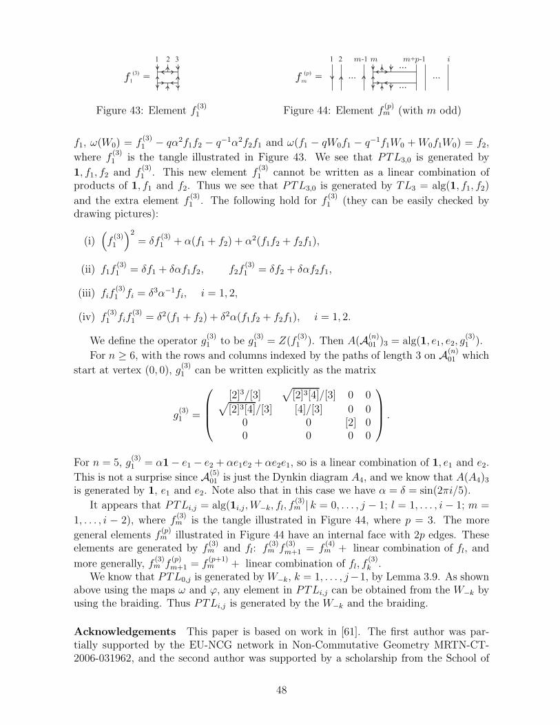
Figure 43: Element f(3)1 Figure 44: Element f

(p)m (with m odd)

f1, ω(W0) = f(3)1 − qα2f1f2 − q−1α2f2f1 and ω(f1 − qW0f1 − q−1f1W0 +W0f1W0) = f2,

where f(3)1 is the tangle illustrated in Figure 43. We see that PTL3,0 is generated by

1, f1, f2 and f(3)1 . This new element f

(3)1 cannot be written as a linear combination of

products of 1, f1 and f2. Thus we see that PTL3,0 is generated by TL3 = alg(1, f1, f2)

and the extra element f(3)1 . The following hold for f

(3)1 (they can be easily checked by

drawing pictures):

(i)(f(3)1

)2

= δf(3)1 + α(f1 + f2) + α2(f1f2 + f2f1),

(ii) f1f(3)1 = δf1 + δαf1f2, f2f

(3)1 = δf2 + δαf2f1,

(iii) fif(3)1 fi = δ3α−1fi, i = 1, 2,

(iv) f(3)1 fif

(3)1 = δ2(f1 + f2) + δ2α(f1f2 + f2f1), i = 1, 2.

We define the operator g(3)1 to be g

(3)1 = Z(f

(3)1 ). Then A(A

(n)01 )3 = alg(1, e1, e2, g

(3)1 ).

For n ≥ 6, with the rows and columns indexed by the paths of length 3 on A(n)01 which

start at vertex (0, 0), g(3)1 can be written explicitly as the matrix

g(3)1 =

[2]3/[3]√

[2]3[4]/[3] 0 0√[2]3[4]/[3] [4]/[3] 0 0

0 0 [2] 00 0 0 0

.

For n = 5, g(3)1 = α1− e1 − e2 + αe1e2 + αe2e1, so is a linear combination of 1, e1 and e2.

This is not a surprise since A(5)01 is just the Dynkin diagram A4, and we know that A(A4)3

is generated by 1, e1 and e2. Note also that in this case we have α = δ = sin(2πi/5).

It appears that PTLi,j = alg(1i,j,W−k, fl, f(3)m | k = 0, . . . , j − 1; l = 1, . . . , i− 1; m =

1, . . . , i − 2), where f(3)m is the tangle illustrated in Figure 44, where p = 3. The more

general elements f(p)m illustrated in Figure 44 have an internal face with 2p edges. These

elements are generated by f(3)m and fl: f

(3)m f

(3)m+1 = f

(4)m + linear combination of fl, and

more generally, f(3)m f

(p)m+1 = f

(p+1)m + linear combination of fl, f

(3)k .

We know that PTL0,j is generated byW−k, k = 1, . . . , j−1, by Lemma 3.9. As shownabove using the maps ω and ϕ, any element in PTLi,j can be obtained from the W−k byusing the braiding. Thus PTLi,j is generated by the W−k and the braiding.

Acknowledgements This paper is based on work in [61]. The first author was par-tially supported by the EU-NCG network in Non-Commutative Geometry MRTN-CT-2006-031962, and the second author was supported by a scholarship from the School of

48

Mathematics, Cardiff University. We thank the referees for their helpful comments. Weare grateful to one of the referees for suggesting the use of the braiding in the proof ofLemma 3.9, which allowed for a simpler proof.

References

[1] F. A. Bais J. K. and Slingerland, Condensate-induced transitions between topologi-cally ordered phases, Phys. Rev. B 79 (2009), 045316, 27 pages.

[2] T. Banica, The planar algebra of a coaction, J. Operator Theory 53 (2005), 119–158.

[3] R. E. Behrend, P. A. Pearce, V. B. Petkova and J.-B. Zuber, Boundary conditionsin rational conformal field theories, Nuclear Phys. B 579 (2000), 707–773.

[4] S. Bigelow, Skein theory for the ADE planar algebras, J. Pure Appl. Algebra 214

(2010), 658–666. arXiv:0903.0144 [math.QA].

[5] S. Bigelow, S. Morrison, E. Peters and N. Snyder, Constructing the extendedHaagerup planar algebra, 2009. arXiv:0909.4099 [math.OA].

[6] D. Bisch, P. Das and S. K. Ghosh, The planar algebra of group-type subfactors, J.Funct. Anal. 257 (2009), 20–46. arXiv:0807.4134 [math.OA].

[7] D. Bisch, P. Das and S. K. Ghosh, The planar algebra of diagonal subfactors, 2008.arXiv:0811.1084 [math.OA].

[8] D. Bisch and V. Jones, Singly generated planar algebras of small dimension, DukeMath. J. 101 (2000), 41–75. II, Adv. Math. 175 (2003), 297–318.

[9] J. Bockenhauer and D. E. Evans, Modular invariants, graphs and α-induction fornets of subfactors. I, Comm. Math. Phys. 197 (1998), 361–386.

[10] J. Bockenhauer and D. E. Evans, Modular invariants, graphs and α-induction fornets of subfactors. II, Comm. Math. Phys. 200 (1999), 57–103.

[11] J. Bockenhauer and D. E. Evans, Modular invariants, graphs and α-induction fornets of subfactors. III, Comm. Math. Phys. 205 (1999), 183–228.

[12] J. Bockenhauer and D. E. Evans, Modular invariants from subfactors, in Quan-tum symmetries in theoretical physics and mathematics (Bariloche, 2000), Contemp.Math. 294, 95–131, Amer. Math. Soc., Providence, RI, 2002.

[13] J. Bockenhauer, D. E. Evans and Y. Kawahigashi, Chiral structure of modular in-variants for subfactors, Comm. Math. Phys. 210 (2000), 733–784.

[14] A. Bruguieres, Categories premodulaires, modularisations et invariants des varietesde dimension 3, Math. Ann. 316 (2000), 215–236.

[15] T. Brzezinski and J. Katriel, Representation-theoretic derivation of the Temperley-Lieb-Martin algebras, J. Phys. A 28 (1995), 5305–5312.

49

[16] E. Date, M. Jimbo, T. Miwa and M. Okado, Solvable lattice models, in Thetafunctions—Bowdoin 1987, Part 1 (Brunswick, ME, 1987), Proc. Sympos. Pure Math.49, 295–331, Amer. Math. Soc., Providence, RI, 1989.

[17] P. Di Francesco and J.-B. Zuber, SU(N) lattice integrable models associated withgraphs, Nuclear Phys. B 338 (1990), 602–646.

[18] L. Dixon, J. A. Harvey, C. Vafa, and E. Witten, Strings on orbifolds. Nuclear Phys.B 261 (1985), 678–686. Nuclear Phys. B 274 (1986), 285–314.

[19] D. E. Evans and Y. Kawahigashi, Orbifold subfactors from Hecke algebras, Comm.Math. Phys. 165 (1994), 445–484.

[20] D. E. Evans and Y. Kawahigashi, Quantum symmetries on operator algebras, OxfordMathematical Monographs. The Clarendon Press Oxford University Press, New York,1998. Oxford Science Publications.

[21] D. E. Evans and M. Pugh, Ocneanu Cells and Boltzmann Weights for the SU(3)ADE Graphs, Munster J. Math. 2 (2009), 95-142. arXiv:0906.4307 [math.OA].

[22] D. E. Evans and M. Pugh, SU(3)-Goodman-de la Harpe-Jones subfactors and therealisation of SU(3) modular invariants, Rev. Math. Phys. 21 (2009), 877–928.arXiv:0906.4252 [math.OA].

[23] D. E. Evans and M. Pugh, A2-Planar Algebras II: Planar Modules. Preprint,arXiv:0906.4311 [math.OA].

[24] P. Fendley and P. Ginsparg, Noncritical orbifolds, Nuclear Phys. B 324 (1989), 549–580.

[25] B. Gato-Rivera and A.N. Schellekens, Complete classification of modular invariantsfor RCFT’s with a center (Zp)

k, Comm. Math. Phys. 145 (1992), 85–121.

[26] S. K. Ghosh, Higher exchange relations, Pacific J. Math. 210 (2003), 299–316.

[27] S. K. Ghosh, Representations of group planar algebras, J. Funct. Anal. 231 (2006),47–89.

[28] A. Guionnet, V. F. R. Jones and D. Shlyakhtenko, Random Matrices, Free Proba-bility, Planar Algebras and Subfactors, 2007. arXiv:0712.2904 [math.OA].

[29] V. P. Gupta, Planar Algebra of the Subgroup-Subfactor, Proc. Indian. Acad. Sci.Math. Sci. 118 (2008), 583-612. arXiv:0806.1791 [math.OA].

[30] V. F. R. Jones, Index for subfactors, Invent. Math. 72 (1983), 1–25.

[31] V. F. R. Jones, Planar algebras. I, New Zealand J. Math. (to appear).

[32] V. F. R. Jones, The planar algebra of a bipartite graph, in Knots in Hellas ’98(Delphi), Ser. Knots Everything 24, 94–117, World Sci. Publ., River Edge, NJ, 2000.

50

[33] V. F. R. Jones, The annular structure of subfactors, in Essays on geometry andrelated topics, Vol. 1, 2, Monogr. Enseign. Math. 38, 401–463, Enseignement Math.,Geneva, 2001.

[34] V. F. R. Jones and D. Penneys, The embedding theorem for finite depth subfactorplanar algebras, 2010. arXiv:1007.3173 [math.OA].

[35] V. F. R. Jones and S. A. Reznikoff, Hilbert space representations of the annularTemperley-Lieb algebra, Pacific J. Math. 228 (2006), 219–249.

[36] V. F. R. Jones, D. Shlyakhtenko and K. Walker, An Orthogonal Approach to theSubfactor of a Planar Algebra, 2008. arXiv:0807.4146 [math.OA].

[37] L. H. Kauffman, State models and the Jones polynomial, Topology 26 (1987), 395–407.

[38] L. H. Kauffman, Knots and physics, Series on Knots and Everything 1, World Sci-entific Publishing Co. Inc., River Edge, NJ, 2001.

[39] V. Kodiyalam, Z. Landau and V. S. Sunder, The planar algebra associated to a Kacalgebra, Proc. Indian Acad. Sci. Math. Sci. 113 (2003), 15–51.

[40] V. Kodiyalam and V. S. Sunder, The planar algebra of a semisimple and cosemisimpleHopf algebra, Proc. Indian Acad. Sci. Math. Sci. 116 (2006), 443–458.

[41] V. Kodiyalam and V. S. Sunder, From Subfactor Planar Algebras to Subfactors,Internat. J. Math. 20 (2009) 1207–1231. arXiv:0807.3704 [math.OA].

[42] V. Kodiyalam and S. Tupurani, Universal skein theory for finite depth subfactorplanar algebras, 2010. arXiv:1003.4577 [math.OA]. A note on generators for finitedepth subfactor planar algebras, 2010. arXiv:1004.1240 [math.OA].

[43] M. Kreuzer and A.N. Schellekens, Simple currents versus orbifolds with discretetorsion – a complete classification, Nucl. Phys. B411 (1994), 97–121.

[44] G. Kuperberg, Spiders for rank 2 Lie algebras, Comm. Math. Phys. 180 (1996),109–151.

[45] Z. Landau, Exchange relation planar algebras, Proceedings of the Conference onGeometric and Combinatorial Group Theory, Part II (Haifa, 2000), Geom. Dedicata95 (2002), 183–214.

[46] Z. Landau and V. S. Sunder, Planar depth and planar Subalgebras, J. Funct. Anal.195 (2002), 71–88.

[47] P. Martin, Potts models and related problems in statistical mechanics, Series on Ad-vances in Statistical Mechanics 5, World Scientific Publishing Co. Inc., Teaneck, NJ,1991.

[48] J. P. May, Definitions: operads, algebras and modules, in Operads: Proceedings ofRenaissance Conferences (Hartford, CT/Luminy, 1995), Contemp. Math. 202, 1–7,Amer. Math. Soc., Providence, RI, 1997.

51

[49] S. Morrison, E. Peters and N. Snyder, Skein Theory for the D2n Planar Algebras, J.Pure Appl. Algebra 214 (2010) 117–139. arXiv:0808.0764 [math.OA].

[50] M. Muger, Galois theory for braided tensor categories and the modular closure, Adv.Math. 150 (2000), 151–201.

[51] A. Ocneanu, Quantized groups, string algebras and Galois theory for algebras, inOperator algebras and applications, Vol. 2, London Math. Soc. Lecture Note Ser.136, 119–172, Cambridge Univ. Press, Cambridge, 1988.

[52] A. Ocneanu, Quantum Symmetry, differential geometry of finite graphs and classifi-cation of subfactors, University of Tokyo Seminary Notes 45, 1991. (Notes recordedby Y. Kawahigashi)

[53] A. Ocneanu, Paths on Coxeter diagrams: from Platonic solids and singularities tominimal models and subfactors. (Notes recorded by S. Goto), in Lectures on operatortheory, (ed. B. V. Rajarama Bhat et al.), The Fields Institute Monographs, 243–323,Amer. Math. Soc., Providence, R.I., 2000.

[54] A. Ocneanu, Higher Coxeter Systems (2000). Talk given at MSRI.http://www.msri.org/publications/ln/msri/2000/subfactors/ocneanu.

[55] A. Ocneanu, The classification of subgroups of quantum SU(N), in Quantum sym-metries in theoretical physics and mathematics (Bariloche, 2000), Contemp. Math.294, 133–159, Amer. Math. Soc., Providence, RI, 2002.

[56] T. Ohtsuki and S. Yamada, Quantum SU(3) invariant of 3-manifolds via linear skeintheory, J. Knot Theory Ramifications 6 (1997), 373–404.

[57] V. Pasquier, Two-dimensional critical systems labelled by Dynkin diagrams, NuclearPhys. B 285 (1987), 162–172.

[58] E. Peters, A Planar Algebra Construction of the Haagerup Subfactor, 2009.arXiv:0902.1294 [math.OA].

[59] M. Pimsner and S. Popa, Iterating the basic construction, Trans. Amer. Math. Soc.310 (1988), 127–133.

[60] S. Popa, An axiomatization of the lattice of higher relative commutants of a subfactor,Invent. Math. 120 (1995), 427–445.

[61] M. Pugh, The Ising Model and Beyond, PhD thesis, Cardiff University, 2008.

[62] P. Pylyavskyy, A2-web Imminants, Discrete Math. 310 (2010), 2183–2197.

[63] K.-H. Rehren, Space-time fields and exchange fields, Comm. Math. Phys. 132 (1990),461–483.

[64] S. A. Reznikoff, Temperley-Lieb planar algebra modules arising from the ADE planaralgebras, J. Funct. Anal. 228 (2005), 445–468.

52

[65] S. A. Reznikoff, Representations of the odd affine Temperley-Lieb algebra, J. Lond.Math. Soc. (2) 77 (2008), 83–98.

[66] A.N. Schellekens and S. Yankielowicz, Extended chiral algebras and modular invari-ant partition functions, Nucl. Phys. B327 (1989), 673–703.

[67] L. C. Suciu, The SU(3) Wire Model, PhD thesis, The Pennsylvania State University,1997.

[68] H. N. V. Temperley and E. H. Lieb, Relations between the “percolation” and “colour-ing” problem and other graph-theoretical problems associated with regular planarlattices: some exact results for the “percolation” problem, Proc. Roy. Soc. LondonSer. A 322 (1971), 251–280.

[69] A. Wassermann, Operator algebras and conformal field theory. III. Fusion of posi-tive energy representations of LSU(N) using bounded operators, Invent. Math. 133(1998), 467–538.

[70] H. Wenzl, Hecke algebras of type An and subfactors, Invent. Math. 92 (1988), 349–383.

[71] F. Xu, New braided endomorphisms from conformal inclusions, Comm. Math. Phys.192 (1998), 349–403.

53