Cyclic cocycles on twisted convolution algebras

arX

iv:1

103.

0578

v1 [

mat

h.Q

A]

2 M

ar 2

011

Cyclic cocycles on twisted convolution algebras

Eitan Angel∗

Department of Mathematics, University of Colorado, UCB 395,

Boulder, Colorado 80309-0395, USA

March 4, 2011

Abstract

We give a construction of cyclic cocycles on convolution algebras twisted by gerbes overdiscrete translation groupoids. For proper etale groupoids, Tu and Xu in [22] provide a mapbetween the periodic cyclic cohomology of a gerbe-twisted convolution algebra and twistedcohomology groups which is similar to the construction of Mathai and Stevenson in [17]. Whenthe groupoid is not proper, we cannot construct an invariant connection on the gerbe; thereforeto study this algebra, we instead develop simplicial techniques to construct a simplicial curvature3-form representing the class of the gerbe. Then by using a JLO formula we define a morphismfrom a simplicial complex twisted by this simplicial curvature 3-form to the mixed bicomplexcomputing the periodic cyclic cohomology of the twisted convolution algebras.

Contents

1 Introduction 2

2 Preliminaries 3

2.1 Categorical notions . . . . . . . . . . . . . . . . . . . . . . . . . . . . . . . . . . . 32.2 Simplicial manifolds . . . . . . . . . . . . . . . . . . . . . . . . . . . . . . . . . . 52.3 Connections and Curvature . . . . . . . . . . . . . . . . . . . . . . . . . . . . . . 72.4 Twisted simplicial cohomology . . . . . . . . . . . . . . . . . . . . . . . . . . . . 8

3 S1-gerbes 10

3.1 Etale groupoids . . . . . . . . . . . . . . . . . . . . . . . . . . . . . . . . . . . . . 103.2 S1-gerbes over etale groupoids . . . . . . . . . . . . . . . . . . . . . . . . . . . . 11

3.2.1 S1-gerbes over discrete translation groupoids . . . . . . . . . . . . . . . . 12

4 Simplicial Curvature 3-form 13

4.1 Twisted bundles . . . . . . . . . . . . . . . . . . . . . . . . . . . . . . . . . . . . 134.2 Derivations ∇k . . . . . . . . . . . . . . . . . . . . . . . . . . . . . . . . . . . . . 164.3 Simplicial 2-form . . . . . . . . . . . . . . . . . . . . . . . . . . . . . . . . . . . . 184.4 Simplicial curvature 3-form . . . . . . . . . . . . . . . . . . . . . . . . . . . . . . 23

∗Email: [email protected]

1

http://arxiv.org/abs/1103.0578v1

5 Cocycles on the twisted convolution algebra 25

5.1 Twisted Convolution Algebra . . . . . . . . . . . . . . . . . . . . . . . . . . . . . 265.2 JLO morphism . . . . . . . . . . . . . . . . . . . . . . . . . . . . . . . . . . . . . 265.3 Algebraic morphisms . . . . . . . . . . . . . . . . . . . . . . . . . . . . . . . . . . 33

1 Introduction

When a manifold M carries the action of a discrete group Γ a natural question to ask is whatthe orbit space M/Γ looks like. In general the orbit space is not a manifold or even a Hausdorffspace. The prescription of Connes’ noncommutative geometry to deal with such “bad” quotientsis to instead study the algebra C∞

c (M ⋊ Γ) of smooth functions with compact support onM × Γ with the discrete convolution product. In [7], Chapter III.2, Connes describes thecyclic cohomology of the convolution algebra C∞

c (M ⋊ Γ) via a morphism Φ from the Bottcomplex of [1] computing the Borel model of equivariant cohomology H∗

Γ(M ;C) = H∗(MΓ;C),where MΓ = M ×Γ EΓ, to the (b, B)-bicomplex computing the periodic cyclic cohomology ofC∞

c (M ⋊ Γ), HP ∗(C∞c (M ⋊ Γ)).

The main result of this paper is the construction of a morphism analogous to Connes’ Φmap into the (b, B)-bicomplex computing the periodic cyclic cohomology of the convolutionalgebra twisted by a gerbe over a discrete translation groupoid. Such a morphism, given by aJLO-type formula, was constructed by Tu and Xu in [22] for the case of a gerbe over any properetale groupoid. Our construction removes the properness requirement in the case of a discretetranslation groupoid. A related construction was also given by Mathai and Stevenson in [17] fora canonical smooth subalgebra of stable continuous trace C∗-algebras having smooth manifoldsas their spectrum (see also [18]). In both [22] and [17] the morphisms constructed are in factisomorphisms whereas the morphism constructed in this paper is in general not an isomorphism.

A presentation of an S1-gerbe over the discrete translation groupoid M ⋊Γ is given by a linebundle L→M ⋊Γ as well as a collection of line bundle isomorphisms µg1,g2 : Lg1 ⊗ (Lg2)

g1 ∼−→

Lg1g2 for every g1, g2 ∈ Γ, where Lg denotes the restriction of L to Mg = M × g. Gerbeswere introduced by J. Giraud [12] and largely developed in a differential geometric frameworkby J.-L. Brylinski [5] to study central extensions of loop groups, line bundles on loop spaces,and the Dirac monopole among other applications. The appearance of gerbes in string theoryand quantum field theory has been studied by numerous mathematicians and physicists, e.g., in[3], [11] and [6]. Sections of L with the convolution product

(f1 ∗ f2)(x, g) =∑

g1g2=g

µg1,g2(f1|Mg1⊗ (f2|Mg2

)g1)(x, g).

define the twisted convolution algebra C∞c (M ⋊ Γ, L).

In the improper case, one cannot construct a Γ-invariant connection on L → M ⋊ Γ as isdone in [22]. In particular, this means that we cannot in general choose a connection ∇ onL→M ⋊ Γ that satisfies the cocycle condition

µ∗g,h(∇gh) = ∇g ⊗ 1 + 1⊗ (∇h)

g

where ∇g denotes ∇|Mg. Instead, there is some discrepancy α ∈ Ω1((M ⋊ Γ)(2))

µ∗g,h(∇g.h)−∇g ⊗ 1 + 1⊗ (∇h)

g = α(g, h).

The curvature forms of ∇g, θg ∈ Ω2(M), define a form θ ∈ Ω2((M ⋊ Γ)(1)). The θg satisfy

θg − θgh + θgh = −dα(g, h)

so that (α, θ) is a cocycle that represents the Dixmier-Douady class in the cohomology of theBott complex of M ⋊ Γ.

2

To overcome this difficulty, the geometric data which forms the source of our morphism isconstructed using simplicial differential forms on the simplicial manifold (M ⋊Γ)•, the nerve ofM ⋊ Γ. The geometric data we use is a complex termed the twisted simplicial complex

(Ω((M ⋊ Γ)•)[u]∗, dΘu

)

where Ω(M•)[u]∗ is a rescaled version of the complex of compatible forms Ω∗(M•) described by

Dupont in [9], u is a formal variable, and dΘuis the de Rham differential twisted by a rescaled

version of the simplicial curvature 3-form Θ in Ω3((M ⋊ Γ)•) which is a representative of theDixmier-Douady class. The 3-form Θ is constructed from the gerbe datum (L, µ,∇), . FromL → M ⋊ Γ we define an infinite dimensional vector bundle E → M as the direct sum bundleE =

⊕g∈Γ Lg with the direct sum connection ∇E . Then EndE →M is a vector bundle of finite

rank endomorphisms over M .From the gerbe datum (L, µ,∇) we define connections ∇k on the vector bundles Ek ×∆k →

(M⋊Γ)(k)×∆k, where Ek = p∗kE and pk : M×Γk →M is the map pk : (m, g1, . . . , gk) 7→ m ∈M .

While End Ek → (M ⋊ Γ)(k) forms a simplicial vector bundle, the sequence of End Ek-valued 2-

forms defined by (∇k)2 do not define a simplicial form. Instead we are able to define a simplicial2-form by the formula

ϑ(k)(g1, . . . , gk) = (∇k)2 −k∑

i=1

tiθg1···gi +∑

1≤i<j≤k

α(g1 · · · gi, gi+1 · · · gj)(tidtj − tjdti).

Here the difference between ϑ(k) and (∇k)2 is a scalar valued form. The simplicial curvature

3-form Θu is defined by (Θu)(k) = ∇ku(ϑu)(k), where ∇

ku and ϑu are rescaled versions of ∇k and

ϑ.A simplicial version of the character formula of A. Jaffe, A. Lesniewski, and K. Osterwalder

[15], similar to [17] and [13] defines a morphism into group cochains valued in the (b, B) bicom-plex of sections of EndE ,

τ∇ : (Ω(M•)[u]•, dΘu

) // (C•(Γ, CC•(Γ∞c (End E))[u−1, u]), b+ uB + δΓ

′).

Following this we define algebraic morphisms

(C•(Γ, CC•(Γ∞c (EndE))[u−1, u]), b+ uB + δΓ

′) // CC•(C∞c (M ⋊ Γ, L)[u−1, u], b+ uB)

into the periodic cyclic complex of the twisted convolution algebra C∞c (M ⋊ Γ, L).

The rest of this paper is organized as follows. The content of Section 2 is a review ofsimplicial notions and the definition of the twisted simplicial complex (Ω((M ⋊ Γ)•)[u]

∗, dΘu).

In Section 3 we discuss gerbes on translation groupoids. Section 4 describes the constructionof the simplicial curvature 3-form Θu. Finally, Section 5 contains the main result, a morphismfrom the twisted simplicial complex of a gerbe datum (L, µ,∇) on M ⋊ Γ to the periodic cycliccomplex of the twisted convolution algebra C∞

c (M ⋊ Γ, L).Acknowledgements. I would like to thank my advisor, Alexander Gorokhovsky, for his

advice, support, and patience. I would also like to thank Arlan Ramsay for his useful suggestionsand helpful discussions.

2 Preliminaries

2.1 Categorical notions

Definition 2.1. The simplicial category ∆ is the small category of objects [n], where [n] is theordered set of n + 1 points, [n] = 0 < 1 < · · · < n, n ∈ N, and arrows the nondecreasingmaps f : [n] → [m]. For n,m ∈ N, a map f : [n] → [m] is called nondecreasing if f(i) ≥ f(j)whenever i > j.

3

Definition 2.2. In ∆ the face maps are the injections δni : [n − 1] → [n], 0 ≤ i ≤ n, which

skip over the ith point, i.e. such that δni (i− 1) = i− 1, δni (i) = i+ 1. The degeneracy maps arethe surjections σ

nj : [n + 1] → [n], 0 ≤ j ≤ n, that sends both j and j + 1 to j, i.e. such that

σnj (j) = σ

nj (j + 1) = j. When the context is clear, we will omit the superscript n.

Definition 2.3. A simplicial object (respectively cosimplicial object) in a category C is a con-travariant functor X• : ∆ → C (respectively a covariant functor X• : ∆ → C). We will oftendenote the objects Xn = X([n]), n ∈ N, and the morphisms δni = X•(δ

ni ) and σn

j = X•(σnj ),

0 ≤ i, j ≤ n. Such a functor is determined entirely by the objects Xn and the morphisms dniand snj (see e.g. [16]). When the morphisms snj are not specified, the functor is instead called apre-simplicial object.

A contravariant functor X• : ∆ → Sets to the category of sets is called a simplicial set. Acontravariant functor X• : ∆→ Top to the category of topological spaces is called a simplicial

space. A contravariant functor X• : ∆→Man to the category of smooth manifolds is called asimplicial manifold (see Section 2.2).

Definition 2.4. The geometric n-simplex is the cosimplicial space ∆• : ∆ → Top defined by∆•([n]) = ∆n, where ∆n is the standard n-simplex

∆n =

(t0, . . . , tn) ∈ Rn+1 : 0 ≤ ti ≤ 1, 0 ≤ i ≤ n,

n∑

i=0

ti = 1

(barycentric) (1)

=

(t1, . . . , tn) ∈ Rn : t1, . . . , tn ≥ 0,

n∑

i=1

ti ≤ 1

(Cartesian). (2)

The Cartesian coordinates may be obtained from the barycentric coordinates eliminating t0 =1− t1 − · · · − tn. For barycentric coordinates

∆•(δni )(t0, . . . , tn−1) = (t0, . . . , ti−1, 0, ti, . . . , tn−1) (3)

∆•(σnj )(t0, . . . , tn+1) = (t0, . . . , tj−1, tj + tj+1, . . . , tn+1), (4)

and for Cartesian coordinates

∆•(δni )(t1, . . . , tn−1) =

(1− t1 − · · · − tn−1, t1, . . . , tn−1) i = 0

(t1, . . . , ti−1, 0, ti, . . . , tn−1) 1 ≤ i ≤ n(5)

∆•(σnj )(t1, . . . , tn+1) =

(t2, . . . , tn+1) i = 0

(t1, . . . , tj + tj+1, . . . , tn+1) 1 ≤ i ≤ n(6)

We will denote ∂ni = ∆•(δni ) and ςnj = ∆•(σn

j ).

Definition 2.5. Given a simplicial set (or space or manifold) X•, the fat realization of X•,denoted ‖X•‖, is the space

‖X•‖ =⋃

n≥0

Xn ×∆n/ ∼ (7)

where ∼ is the equivalence relation generated by (δni (x), t) ∼ (x, ∂ni (t)), for (x, t) ∈ Xn ×∆n−1.

The geometric realization of X , denoted by |X | is the space

|X•| =⋃

n≥0

Xn ×∆n/ ≈ (8)

where ≈ is the equivalence relation generated by (f∗(x), t) ≈ (x, f∗(t)) for (x, t) ∈ Xn ×∆n−1

and any f ∈ hom(∆).

Definition 2.6. Let C(n) consist of n-tuples of composable arrows in a (small) category C, withC(0) the objects of C. The nerve of C is the simplicial set C• : ∆ → Sets given on objects by

4

C•([n]) = C(n) and on morphisms by the faces C•(δni ) = δni which compose adjacent morphisms

in the ith place and by the degeneracies C•(σnj ) = σn

j which insert the identity morphism in the

jth place, i.e.

δni (f1, . . . , fn) =

(f2, . . . , fn) if i = 0

(f1, . . . , fifi+1, . . . , fn) for 1 ≤ i ≤ n− 1

(f1, . . . , fn−1) if i = n

(9)

σnj (f1, . . . , fn) = (f1, . . . , fj , id, fj+1, . . . , fn) (10)

with δ10(f) the terminal object of f and δ11(f) the initial object of f and where fifi+1 = fi+1 fi.The classifying space BC of the small category C is the geometric realization of the nerve of C.

2.2 Simplicial manifolds

We will now recount the ideas of Dupont in [9] (and [10]) to explicitly construct the cohomologyof a simplicial manifold.

Definition 2.7. Given a simplicial manifold M• : ∆ → Man, a simplicial differential k-formon M• is a sequence of k-forms ω(n), where ω(n) ∈ Ωk(Mn × ∆n), and which satisfy thecompatibility condition

(id× ∂i)∗ω(n) = (δi × id)∗ω(n−1) (11)

on Ωk(Mn ×∆n−1) for all 0 ≤ i ≤ n and n ≥ 1. The complex (Ω∗(M•), d) of compatible forms

consists of

• the differential graded algebra (dga) of simplicial differential forms on M• form denotedby Ω∗(M•)

• an exterior differentiald : Ωk(M•)→ Ωk+1(M•)

induced by the exterior differentials d : Ωk(Mn × ∆n) → Ωk+1(Mn × ∆n) for all n ∈N. Explicitly, dω(n) = dω(n), which is well defined as the de Rham differential onMn ×∆n−1 respects the compatibility condition (11) for all n ∈ N.

• a wedge product∧ : Ωk(M•)⊗ Ωl(M•)→ Ωk+l(M•)

is induced by the wedge products ∧ : Ωk(Mn×∆n)⊗Ωl(Mn×∆n)→ Ωk+l(Mn×∆n) forall n ∈ N.

Notice that ω(n) defines a k-form on∐

n≥0 Mn × ∆n. In view of this, the compatibilitycondition (11) is precisely the condition required for ω(n) to define a form on ‖M•‖.

Definition 2.8. We may think of the complex (Ω∗(M•), d) as a bicomplex (Ωr,s(M•), ddR, d′∆)

called the bicomplex of compatible forms such that

(Ω∗(M•), d) = Tot (Ωr,s(M•), ddR, d′∆). (12)

The bicomplex of compatible forms consists of

• simplicial (r + s)-forms on M•

Ωr,s(M•) =

∐

n≥0

Ωr(Mn)⊗ Ωs(∆n)

/∼ (13)

where ∼ is essentially the compatibility condition (11). Explicitly, if ωr,s(n) ∈ Ωr(Mn) ⊗

Ωs(∆n) we may write ωr,s(n) as a linear combination of forms αr

(n)⊗βs(n) where α

r(n) ∈ Ωr(Mn)

and βs(n) ∈ Ωs(∆n). Then ∼ is defined by

αr(n) ⊗ βs

(n) ∼ αr(n−1) ⊗ βs

(n−1) ⇐⇒ αr(n) ⊗ ∂∗

i (βs(n)) = δ∗i (α

r(n−1))⊗ βs

(n−1), (14)

5

• a differentialddR = d : Ωr,s(M•)→ Ωr+1,s(M•) (15)

induced by the collection of exterior differentials on each Mn,

d⊗ id : Ωr(Mn)⊗ Ωs(∆n)→ Ωr+1(Mn)⊗ Ωs(∆n), (16)

for all n ∈ N.

• a differentiald′∆ = (−1)rd : Ωr,s(M•)→ Ωr,s+1(M•) (17)

induced by the collection of exterior differentials on each ∆n,

id⊗ d : Ωr(Mn)⊗ Ωs(∆n)→ Ωr(Mn)⊗ Ωs+1(∆n), (18)

for all n ∈ N.

As before, the induced differentials on Ωr,s(M•) are well defined as a result of the compat-ibility condition (14). With this notation the complex of compatible forms may be written(Ω∗(M•), ddR + d′∆).

As the dga of compatible forms carries a bigrading,

Ωk(M•) =⊕

r+s=k

Ωr,s(M•), (19)

given an element of the complex of of compatible forms ω ∈ Ωk(M•) we will denote the compo-nent of ω in Ωr,s(M•) by

ωr,s = ω|Ωr,s(M•). (20)

The (r + s)-forms of Ωr,s(M•) have a local description as

ωr,s|Mn×∆n =∑

ωi1···irj1···jsdxi1 ∧ · · · ∧ dxir ∧ dtj1 ∧ · · · ∧ dtjs (21)

where xi are local coordinates of Mn and (t0, . . . , tn) are barycentric coordinates of ∆n.

Definition 2.9. The simplicial de Rham complex (A∗(M•), δ + d′) is defined by

Ak(M•) =⊕

r+s=k

Ar,s(M•) (22)

where

• Ar,s(M•) = Ωs(Mr) is the collection of differential s-forms on the manifold Mr,

• the differentialδ : Ar,s(M•)→ A

r+1,s(M•) (23)

is the alternating sum of the pullback of the face maps δr+1i = M•(δ

ni ), 0 ≤ i ≤ r + 1,

• the differentiald′ : Ar,s(M•)→ A

r,s+1(M•) (24)

is the exterior differential (−1)rd : Ωs(Mr)→ Ωs+1(Mr).

Then we have(A∗(M•), δ + d′) = Tot (Ar,s(M•), δ, d

′). (25)

Definition 2.10. Given a commutative ring R, the simplicial singular cochain complex associ-ated to a simplicial manifold M• is denoted (C∗(M•;R), δ + ∂′) and consists of

• the spaces

Ck(M•;R) =⊕

r+s=k

Cr,s(M•;R) (26)

where Cr,s(M•;R) = Cs(Mr;R) is the space of singular cochains of degree s on Mr,

6

• the differentialδ : Cr,s(M•;R)→ Cr+1,s(M•;R) (27)

is the alternating sum of the pullback of the face maps δr+1i = M•(δ

ni ), for all 0 ≤ i ≤ r+1,

• and∂′ : Cr,s(M•;R)→ Cr,s+1(M•;R) (28)

is (−1)r times the usual coboundary on singular cochains.

Then we have(C∗(M•;R), δ + ∂′) = Tot (Cr,s(M•;R), δ, ∂′). (29)

From [9] Proposition 5.15

Theorem 2.11. For a simplicial manifold M•, we have the isomorphism

H∗(‖M•‖;R) ∼= H(C∗(M•;R), δ + ∂′) (30)

and from [9] Proposition 6.1,

Theorem 2.12 (Simplicial de Rham theorem). The integration map

I : Ar,s(M•)→ Cr,s(M•) (31)

defined by I(ωr,s)(cr,s) =∫cr,s

ωr,s for ωr,s ∈ Ar,s(M•) and cr,s ∈ Cs(Mr), the collection of

singular s-chains on Mr, gives a morphism of double complexes. Furthermore, this integration

map induces an isomorphism

H(A∗(M•), δ + d′) ∼= H(C∗(M•), δ + ∂′) (32)

on cohomology.

Furthermore, there is another morphism of complexes given by Stokes’ theorem. From [9]Theorem 6.4,

Theorem 2.13. Let

I∆ : (Ωr,s(M•), ddR, d∆)→ (Ar,s(M•), δ, d′) (33)

be the map defined by integration over the standard simplex, i.e. the map defined on Ωs(Mr×∆r)

by

I∆ : ω(r) 7→

∫

∆r

ω(r). (34)

Then I∆ is a morphism that induces an isomorphism

H(Ω∗(M•), d′) ∼= H((A∗(M•), δ + d′) (35)

2.3 Connections and Curvature

Definition 2.14. Let G be a Lie group. A simplicial G-bundle π• : E• →M• over a simplicialmanifold M• is a sequence of principal G-bundles πn : En →Mn where E• is itself a simplicialmanifold and the diagrams

En+1En+1(δi)

//

πn+1

En

πn

En−1En−1(σj)

//

πn−1

En

πn

Mn+1Mn+1(δi)

// Mn and Mn−1Mn−1(σj)

// Mn

(36)

commute. Given a simplicial G-bundle π• : E• → M•, the geometric realization |π•| : |E•| →|M•| is a principal G-bundle with G-action induced by

En ×∆n ×G→ En ×∆n, (x, t, g) 7→ (xg, t). (37)

If we only require that the first diagram of (36) commute then we may still consider the fatrealization ‖π•‖ : ‖E•‖ → ‖M•‖ which is a principal G-bundle.

7

Definition 2.15. A connection in a simplicial G-bundle π• : E• →M• is a 1-form ω ∈ Ω1(E•; g)on E• (in the sense of definition 2.7) with coefficients in g, the Lie algebra of G, such thatω(n) = ω|En×∆n is a connection in the usual sense on the bundle πn× id : En×∆n →Mn×∆n.The curvature θ of a connection ω is the differential form

θ = dω +1

2[ω, ω] ∈ Ω2(M•; g). (38)

2.4 Twisted simplicial cohomology

In this section we will construct a twisted version of the complex of compatible forms, althoughrather than using forms, this construction will be based on densities. We will first define a versionof the de Rham complex of a manifold twisted by a 3-form in preparation for the definition ofthe de Rham complex of a simplicial manifold twisted by a simplicial 3-form.

For τ the orientation bundle of a manifold M , let Ω∗τ (M) be the densities of M . The

cohomology of the τ-twisted de Rham complex, (Ω∗τ (M), d), is the τ-twisted de Rham cohomology,

H∗τ (M). The τ-twisted de Rham cohomology with compact support, H∗

τ,c(M) is defined similarly.For more details, see [2] Chapter I.7.

In the following, let u be a formal variable of degree +2.

Definition 2.16. Given a smooth manifold M and a closed 3-form Θ ∈ Ω3(M), the Θ-twisted

de Rham complex of M , denoted by (Ω(M)[u]•, dΘ), is defined as follows.

• DefineΩk(M) := ΩdimM−k

τ (M). (39)

Let Ω(M)[u]k denote polynomials in u over Ω∗(M) such that the degree in Ω∗(M) plusthe degree of powers of u sum to k. In other words elements ω ∈ Ω(M)[u]k are linearcombinations of ujωℓ for any ωℓ ∈ Ωℓ(M) such that 2j + ℓ = k, for all 0 ≤ ℓ ≤ dimM .

• Note the de Rham differential

ddR : Ωk(M)→ Ωk−1(M) (40)

is of degree −1 and exterior multiplication by Θ,

Θ ∧ · : Ωk(M)→ Ωk−3(M) (41)

is of degree −3. We can rescale the de Rham differential by u to obtain a degree +1differential

uddR : Ω(M)[u]k → Ω(M)[u]k+1. (42)

The differentialdΘ := uddR + u2Θ ∧ · : Ω(M)[u]k → Ω(M)[u]k+1 (43)

is of degree +1.

The cohomology of (Ω(M)[u]•, dΘ) is called the Θ-twisted cohomology of M , denoted H∗Θ(M).

If Θ′ = Θ+dη is cohomologous to Θ then the complexes (Ω(M)[u]•, dΘ) and (Ω(M)[u]•, dΘ′)are isomorphic via the isomorphism

Iη : ξ 7→ e−uη ∧ ξ (44)

Now we will similarly describe the de Rham complex of a simplicial manifold M• in which thetwisting of the complex of compatible forms is given by a closed compatible 3-form Θ ∈ Ω3(M•).This definition involves a modification of the bicomplex of compatible forms (13).

Definition 2.17. Given a simplicial manifold M and a closed compatible 3-form Θ ∈ Ω3(M•),the Θ-twisted complex of compatible forms of M•, denoted by (Ω(M•)[u]

•, dΘu), is defined as

follows.

8

• First we adjust the grading of Ωr,s(M•) to define a bicomplex Ω(M•)[u]r,s. Let

Ω(M•)[u]r,s =

∐

n≥0

Ω(Mn)[u]r ⊗ Ωs(∆n)

/∼ (45)

where the equivalence relation ∼ is defined in precisely the same way as the compatibilitycondition in (14). For αr

(n) ∈ Ω(Mn)[u]r and βs

(n) ∈ Ωs(∆n), we have αr(n) ⊗ βs

(n) ∼

αr(n−1) ⊗ βs

(n−1) if and only if the corresponding statement to (14) holds. As in (19), wedefine

Ω(M•)[u]k =

⊕

r+s=k

Ω(M•)[u]r,s. (46)

Note the degrees are such that for a (dimM − ℓ)-form ωℓ ∈ Ωℓ(Mn) and ηs ∈ Ωs(∆n),

ujωℓ ⊗ ηs ∈ (Ω(M•)[u]2j+ℓ,s)|Mn×∆n

• Furthermore, there is a degree +1 differential

uddR : Ω(M•)[u]r,s → Ω(M•)[u]

r+1,s (47)

induced by the exterior derivative on each Mn,

(−1)dimM−r+sud⊗ id : Ω(Mn)[u]r ⊗ Ωs(∆n)→ Ω(Mn)[u]

r+1(Mn)[u]⊗ Ωs(∆n) (48)

and there is a degree +1 differential d∆ induced by the exterior derivative on each ∆n, i.e.

d∆ = id⊗ d : Ω(Mn)[u]r ⊗ Ωs(∆n)→ Ω(Mn)[u]

r ⊗ Ωs+1(∆n). (49)

• Given a compatible differential 3-form Θ ∈ Ω3(M•) as in Definition 2.7 we may decomposeΘ with respect to the sum (19) as Θ = Θ3,0+Θ2,1+Θ1,2+Θ0,3 where Θj,3−j ∈ Ωj,3−j(M•)for 0 ≤ j ≤ 3. If, further, Θ0,3 = 0 then define a rescaling of Θ

Θu = u2Θ3,0 + uΘ2,1 +Θ1,2 ∈ Ω(M•)[u]•. (50)

Hence, exterior multiplication by Θu is an operator of degree +1 on

Θu ∧ · : Ω(M•)[u]k → Ω(M•)[u]

k+1. (51)

• So for a closed, compatible 3-form Θ we define

dΘu:= uddR + d∆ −Θu ∧ · : Ω(M•)[u]

k → Ω(M•)[u]k+1. (52)

The cohomology of (Ω(M•)[u]•, dΘu

) is called the Θ-twisted cohomology of M•, denotedH∗Θ(M•).

Remark 2.18. As the nerve of any Lie groupoid G (see Definition 3.5) defines a simplicial manifoldG•, we may speak of the complex of compatible forms and, given a closed, compatible 3-formΘ, the Θ-twisted complex of compatible forms of G.

Proposition 2.19. Let Θ,Θ′ ∈ Ω3(M•) be compatible forms such that the components in

Ω0,3(M•) satisfy (Θ)0,3 = (Θ′)0,3 = 0. If Θ − Θ′ = dη for some η ∈ Ω2(M•) that satisfies

η0,2 = 0 then (Ω(M•)[u]•, dΘu

) and (Ω(M•)[u]•, dΘ′

u) are isomorphic via the isomorphism

Iη : ξ 7→ e−ηu ∧ ξ (53)

where ηu = uη2,0 + η1,1.

Lemma 2.20. For ω1 ∈ Ω(M•)[u]k and ω2 ∈ Ωℓ(M•)[u] the induced wedge product satisfies

(−1)|ω2|(uddR + d∆)(ω1 ∧ ω2) = ((uddR + d∆)ω1) ∧ ω2 + ω1 ∧ ((uddR + d∆)ω2)

9

Proof. As the variable u is of even degree and will not alter any signs, let d = ddR + d∆ and letd = ddR + d∆. Suppose ω1 ∈ Ω(M•)[u]

r1,s1 and ω2 ∈ Ωr2,s2(M•)[u] so that

d(ω1 ∧ ω2) = (−1)dimM−r1+r2+s1+s2d(ω1 ∧ ω2)

= (−1)dimM−r1+r2+s1+s2(dω1 ∧ ω2 + (−1)dimM−r1+s1ω1 ∧ dω2)

= (−1)dimM−r1+r2+s1+s2((−1)dimM−r1+s1 dω1 ∧ ω2

+(−1)dimM−r1+s1ω1 ∧ dω2

)

= (−1)−r2+s2 dω1 ∧ ω2 + (−1)−r2+s2ω1 ∧ dω2

Since |ω2| = r2 + s2 which is s2 − r2 modulo 2,

d(ω1 ∧ ω2) = (−1)|ω2|dω1 ∧ ω2 + (−1)|ω2|ω1 ∧ dω2

from which the lemma follows.

3 S1-gerbes

3.1 Etale groupoids

We will recall some standard material about groupoids. See [19], [8], or [20] for example.

Definition 3.1. A groupoid is a small category G in which every arrow is invertible. The setof objects is denoted by G(0) and the set of arrows is denoted by G(1). The set of arrows willoften be denoted simply by G. For each arrow in G(1) there is a source object and a range objectgiven by the range and source maps, r, s : G(1) G(0). To denote that g ∈ G(1) is an arrow with

source s(g) = x and range r(g) = y we write either g : x→ y or xg−→ y.

As G is a category, there is a rule of composition. Given two arrows yg1−→ z, x

g2−→ y ∈ G(1)

such that s(g1) = r(g2), their composition is an arrow xg1g2−−−→ z called their product. If we define

pairs of composable arrows as

G(2) = G(1) ×G(0)G(1) = (g1, g2) ∈ G(1) × G(1) : s(g1) = r(g2) (54)

then the product defines the multiplication map

m : G(2) → G(1), m(g1, g2) = g1g2. (55)

As the composition in a category is required to be associative, the groupoid product is associa-tive.

For any object x ∈ G(0) there is an identity morphism 1x : x→ x that satisfies 1xg = g1y = g

for any arrow xg−→ y ∈ G(1). The unit map is then

u : G(0) → G(1), u(x) = 1x.

Every arrow g : x→ y in G(1) is invertible so we will denote the inverse of g by g−1 : y → x.With this we can define the inverse map

i : G(1) → G(1), i(g) = g−1.

Then g−1g = 1x and gg−1 = 1y.

Remark 3.2. As a groupoid G is a category, Definition 2.6 applies and there is a simplicial setG• called the nerve of G.

10

Definition 3.3. As in [4], Section 2.3, we will define the following projection maps. For 0 ≤i ≤ n and G• the nerve of G let prni : G(n) → G(0) be the final object of the ith morphism wheni 6= n and the initial object of the last morphism when i = n. For 0 ≤ j ≤ n, 0 ≤ ij ≤ m,the map prni0 × · · · × prnim : G(n) → (G(0))

m factors into maps G(n) → G(m) and the canonicalprojection G(m) → (G(0))

m. The map G(n) → G(m) will be denoted prni0···im . We may writeprni0···im explicitly as

prni0···im : (g1, . . . , gn) 7→ (g′1, . . . , g′m)

where, for 1 ≤ k ≤ m

g′k =

gik−1+1 · · · gik if ik−1 < ik

ids(gik ) if ik−1 = ik

(gik · · · gik−1−1)−1 if ik−1 > ik

Remark 3.4. The maps δni of Definition 2.6 may be written prn0···i···n

: G(n) → G(n−1) where idenotes the omission of i.

Definition 3.5. A Lie groupoid is a groupoid in which the sets G(0) and G(1) are smoothmanifolds and the structure maps r, s, u, i,m are smooth. Furthermore, the range and sourcemaps r, s : G(1) G(0) are required to be submersions so that the domain of the multiplicationmap, G(2), is a manifold. An etale groupoid is a Lie groupoid in which the source map is etale,i.e. a local diffeomorphism. In this case the other structure maps are etale as well.

Example 3.6. 1. Given a manifold M with an open cover U = Uα, the Cech groupoid

associated to U has objects∐

α Uα and morphisms∐

α,β Uαβ where Uαβ = Uα ∩ Uβ . Therange and source maps are the embeddings r : Uαβ → Uβ and s : Uαβ → Uα.

2. Given a manifold M carrying a right action of a group G, there is a groupoid called thetranslation groupoid or action groupoid M ⋊G with objects (M ⋊G)(0) = M and arrows(M⋊G)(1) = M×G. The source and range maps are given by s(x, g) = xg and r(x, g) = x.

Given arrows xg1g1←− x and xg1g2

g2←− xg1 their composition is m((x, g1), (xg1, g2)) =

(x, g1g2) = xg1g2g1g2←−−− x.

3.2 S1-gerbes over etale groupoids

Definition 3.7. Given an etale groupoid G, a gerbe datum is a triple (L, µ,∇) with

• L a line bundle L→ G over G(1);

• µ an isomorphismµ : (pr201)

∗L⊗ (pr212)∗L

∼−→ (pr202)

∗L (56)

of line bundles over G(2) which satisfies the associativity condition that the diagram

(pr301)∗L⊗ (pr3123)

∗L (pr30123)∗L

(pr3013)∗(µ)

//

(pr301)∗L⊗ (pr312)

∗L⊗ (pr323)∗L

(pr301)∗L⊗ (pr3123)

∗L

id⊗(pr3123)∗(µ)

(pr301)∗L⊗ (pr312)

∗L⊗ (pr323)∗L (pr3012)

∗L⊗ (pr323)∗L

(pr3012)∗(µ)⊗id

// (pr3012)∗L⊗ (pr323)

∗L

(pr30123)∗L

(pr3023)∗(µ)

(57)

commutes. Such an isomorphism may be written as µ(g1,g2) : L|g1 ⊗L|g2∼−→ L|g1g2 on the

fiber over (g1, g2) ∈ G(2). Hence on fibers this condition means that the diagram

L|g1 ⊗ L|g2g3 L|g1g2g3µ(g1,g2g3)

//

L|g1 ⊗ L|g2 ⊗ L|g3

L|g1 ⊗ L|g2g3

id⊗µ(g2,g3)

L|g1 ⊗ L|g2 ⊗ L|g3 L|g1g2 ⊗ L|g3µ(g1,g2)⊗id

// L|g1g2 ⊗ L|g3

L|g1g2g3

µ(g1g2,g3)

(58)

11

commutes.

• ∇ a connection on L→ G. In other words a linear operator ∇ : Γ∞(L)→ Ω1(G, L) whereΓ∞(L) denotes sections of L→ G and Ω1(G, L) denotes L-valued 1-forms on G.

Associated to a gerbe datum (L, µ,∇) on an etale groupoid G there are 3-cocycles in Ω∗(G•)

(α, θ) ∈ Ω1(G(2))⊕ Ω2(G(1)) (59)

where

• α is the discrepancy between the connection (pr201)∗∇⊗ 1 + 1 ⊗ (pr212)

∗∇ on (pr201)∗L ⊗

(pr212)∗L and the connection (µ)∗(pr202)

∗∇ on (µ)∗(pr202)∗L:

(µ)∗(pr202)∗∇−

((pr201)

∗∇⊗ 1 + 1⊗ (pr212)∗∇)= α ∈ Ω1(G(2)) (60)

• θ is any element of Ω2(G(1)) such that

δθ = −dα. (61)

In particular, θ = curv(∇), the curvature of ∇, satisfies (61).

Such an (α, θ) ∈ Ω1(G(2))⊕ Ω2(G(1)) determines a class in H3dR(G), which we call the Dixmier-

Douady class of (L, µ,∇). Although the Dixmier-Douady class depends on ∇ throughout thisarticle, it is expected this dependence can be removed. This notion of a gerbe and Dixmier-Douady class agrees with the notion of a gerbe on a manifold (as in [14]) when G is the Cechgroupoid.

3.2.1 S1-gerbes over discrete translation groupoids

As the rest of this paper is concerned with gerbes on translation groupoids arising from a discretegroup action on a manifold, we will adopt a bit of new notation for this case. Given a discretegroup Γ and a manifold M carrying a (right) action of Γ, M ×Γ→M , denoted (x, g) 7→ xg, theassociated translation groupoid is an etale groupoid and is denoted M ⋊Γ. The nerve of M ⋊Γis a simplicial manifold (M ⋊ Γ)• which is explicitly given on objects by (M ⋊ Γ)(k) = M × Γk

and on morphisms by

δki (m, g1, . . . , gk) =

(mg1, g2, . . . , gk) if i = 0

(m, g1, . . . , gigi+1, . . . , gk) for 1 ≤ i ≤ k − 1

(m, g1, . . . , gk−1) if i = k

(62)

σkj (m, g1, . . . , gk) = (m, g1, . . . , gj, 1Γ, gj+1, . . . , gk) (63)

in the notation of (9). In particular, δ10(m, g1) = mg1 and δ11(m, g1) = m.Let (L, µ,∇) be a presentation of a gerbe on M ⋊ Γ. As (M ⋊ Γ)(1) = M × Γ and Γ is a

discrete group, we may view L as a collection of line bundles Lg on Mg = M × g for eachg ∈ Γ. The isomorphism µ may be restricted in the same way to a collection of isomorphisms

µg1,g2 : Lg1 ⊗ (Lg2)g1 ∼−→ Lg1g2 (64)

where g1, g2 ∈ Γ and (Lg2)g1 denotes the line bundle Lg2 shifted by the action of g1. In

other words (Lg2)g1 has sections sg1 where sg1(x) = s(xg1) denotes the (left) action of Γ for

s ∈ Γ∞(Lg2).Also denote the restriction of ∇ to Lg by ∇g = ∇|Mg

for each g ∈ Γ. In this case thecondition (60) may be written

µ∗g1,g2(∇gh)− (∇g ⊗ 1 + 1⊗ (∇h)

g) = α(g, h) (65)

for all g, h ∈ Γ and for some α(g, h) ∈ Ω1(M). Hence α ∈ Ω1((M ⋊ Γ)(2)).Define θg ∈ Ω2(M) by [θg, s] = (∇g)

2s for a section s : Mg → Lg. Then we have a collectionθ = (θg)g∈Γ ∈ Ω2((M ⋊ Γ)(1)) and the following relation

12

Proposition 3.8. The 2-forms θg satisfy condition (61), which may be written

θg + θgh − θgh = −dα(g, h) (66)

Proof. This follows from condition (65). The curvature of the sum of connections ∇g ⊗ 1 + 1⊗(∇h)

g is θg + θgh and the curvature of the connection minus scalar form µ∗g1,g2(∇gh)− α(g, h) is

θgh − dα(g, h).

4 Simplicial Curvature 3-form

Our goal now will be to construct a 3-form Θ ∈ Ω3((M ⋊ Γ)•) that is a representative of theDixmier-Douady class of (L, µ,∇) in the complex of compatible forms on (M ⋊ Γ)• for a fixedmanifold M carrying the action of a discrete group Γ. Throughout this section, also fix thenotation (L, µ,∇) for a gerbe datum on M ⋊ Γ.

4.1 Twisted bundles

Definition 4.1. An (L, µ,∇)-twisted vector bundle with connection is a triple (E , ϕ,∇E ) where

• E is a vector bundle on M together with

• ϕ = ϕgg∈Γ is a collection of vector bundle isomorphisms ϕg : E∼−→ Eg ⊗ Lg for each

g ∈ Γ such that the diagram

Eg ⊗ Lg Eϕ−1

g

//

Egh ⊗ (Lh)g ⊗ Lg

Eg ⊗ Lg

((ϕh)g)−1⊗id

Egh ⊗ (Lh)g ⊗ Lg Egh ⊗ Lgh

id⊗µg,h// Egh ⊗ Lgh

E

ϕ−1gh

(67)

commutes. Here Eg denotes the vector bundle E shifted by the action of g.

• ∇E : Γ∞(E) // Ω1(M, E) is a connection on E .

Remark 4.2. Note that ϕg induces an isomorphism ϕg : EndE∼−→ End Eg as well. More precisely,

ϕg : E∼−→ Eg ⊗ Lg induces an isomorphism

ϕg : EndE∼−→ End (Eg ⊗ Lg) ∼= End (Eg)⊗ End (Lg).

As End (Lg) ∼= C we see End E ∼= EndEg via ϕg.

Let θ = curv(∇) and denote the discrepancy of (L, µ,∇) by α. Then there is a connectionon Eg ⊗ Lg given by (∇E)

g⊗ 1 + 1 ⊗ ∇g for every g ∈ Γ. By (∇E )

gwe mean the connection

(∇E )gsg = (∇Es)

gwhere sg is a section of Eg. This defines a connection on Eg which we denote

∇Eg

= (∇E)g. The discrepancy between ∇E and ∇Eg

⊗ 1 + 1 ⊗∇g is an End E-valued 1-formwhich we denote by

ϕ∗g(∇

Eg

⊗ 1 + 1⊗∇g)−∇E = A(g) ∈ Ω1(M,End E) (68)

for each g ∈ Γ. We will call A ∈ Ω1(M × Γ,End E) the discrepancy of ∇E . Notice that we thenhave the identity

(∇E +A(g))2 = ϕ∗g((∇

Eg

)⊗ 1 + 1⊗∇g)2

(∇E)2 +A(g)2 + [∇E , A(g)] = ϕ∗g((∇

Eg

)2) + θg

θE +A(g)2 + [∇E , A(g)] = ϕ∗g(θ

E)g + θg (69)

on Ω2(M,End E) where we define θE = (∇E)2.

13

Example 4.3 (Direct Sum Bundle). There is a particular (L, µ,∇)-twisted vector bundle calledthe direct sum bundle of (L, µ,∇) which is the most relevant example of a twisted vector bundlefor our purposes. The direct sum bundle (E , ϕ,∇E ) of (L, µ,∇) consists of

• the (possibly infinite dimensional) vector bundle π : E →M where E =⊕

g∈Γ Lg,

• a collection of isomorphisms ϕ = ϕgg∈Γ with ϕg : E // Eg ⊗ Lg for each g ∈ Γ definedby

ϕg :⊕

g′∈Γ

Lg′//

⊕

g′∈Γ

µ−1g,g−1g′

(Lg′) =⊕

g′∈Γ

(Lg−1g′)g ⊗ Lg (70)

where the factor Lg′ is mapped to µ−1g,g−1g′

(Lg′) under ϕg.

• the direct sum connection ∇E =⊕

g∈Γ∇g on E →M induced by ∇.

Lemma 4.4. Let (E , ϕ,∇) be the direct sum bundle of (L, µ,∇). Then for any g, h ∈ Γ we have

the identity

A(g) + (ϕg)∗(A(h)g)−A(gh) = α(g, h) ∈ Ω1(M,End E), (71)

where α is the discrepancy of ∇ and A is the discrepancy of ∇E .

Proof. This follows from the commutativity of (67).

Lemma 4.5. Let (E , ϕ,∇) be the direct sum bundle of (L, µ,∇). For any g1, . . . , gj ∈ Γ and

1 < i < j,

α(g1, g2 · · · gi)− α(g1, g2 · · · gj) + α(g1 · · · gi, gi+1 · · · gj) = ϕ∗g1α(g2 · · · gi, gi+1 · · · gj)

g1 , (72)

where α is the discrepancy of ∇.

Proof. This follows from a direct calculation using Lemma 4.4.

The bundle End E → M is vector bundle of finite rank endomorphisms when (E , ϕ,∇E ) isa direct sum bundle of (L, µ,∇). Note that any section of Γ∞(End E) may be decomposedas follows. Since E =

⊕g∈Γ Lg, End E consists of morphisms φ :

⊕g∈Γ Lg →

⊕g∈Γ Lg. Let

Eg,h(φ) ∈ Hom(Lg, Lh) denote the restriction of φ to the component Eg,h(φ) : Lg → Lh, sothat φ =

⊕g,h∈Γ Eg,h(φ). So given a section f ∈ Γ∞(End E) we may decompose f in the

same way, with Eg,h(f) a section on M with values in morphisms Lg → Lh. In other words,Eg,h(f) ∈ Γ∞(Hom (Lg, Lh)).

Given such a decomposition we can describe the action of g ∈ Γ on sections Γ∞(End E) asfollows. Let f ∈ Γ∞(Hom (Lg1 , Lg2)), i.e. f = Eg1,g2(f). For any g ∈ Γ, the section fg is asection of Hom (Lg

g1 , Lgg2) and id ⊗ fg is a section of Hom (Lg ⊗ (Lg1)

g, Lg ⊗ (Lg2)g). We may

denote the corresponding section by fg as well. As there are isomorphisms µg,g1 : Lg⊗(Lg1)g →

Lgg1 and µg,g2 : Lg ⊗ (Lg2)g → Lgg2 , under these isomorphisms fg corresponds to a section in

Γ∞(Hom (Lgg1 , Lgg2)) which is denoted by Egg1,gg2 (fg). In other words

Egg1,gg2(fg) = µg,g2 id⊗ fg µ−1

g,g1

Hence the (left) action of g ∈ Γ on Eg1,g2(f) is g · Eg1,g2(f) = Egg1,gg2(fg).

For a section a ∈ Γ∞(Lg), we may consider a as the section E1,g(a) : L1 → Lg of Γ∞(End E)since a : Mg → Lg defines a section a : M × C → Lg by a(x, λ) = a(x) for all λ ∈ C and

L1∼= M × C. We have L1

∼= M × C as µ1,1 : L1 ⊗ L1∼−→ L1. We will not make a distinction in

notation between a section a : M → Lg and the corresponding section of Γ∞(Hom (L1, Lg)).Let f1, f2 ∈ Γ∞(End E) be sections of EndE . The sections Eg1,g2(f1) and Eg2,g3(f2) may

be composed to produce a section Eg2,g3(f2) Eg1,g2(f1). We will denote this operation ofcomposition by

Eg1,g2(f1)Eg2,g3(f2) = Eg1,g3(f1f2) ∈ Γ∞(Hom (Lg1 , Lg3)) (73)

14

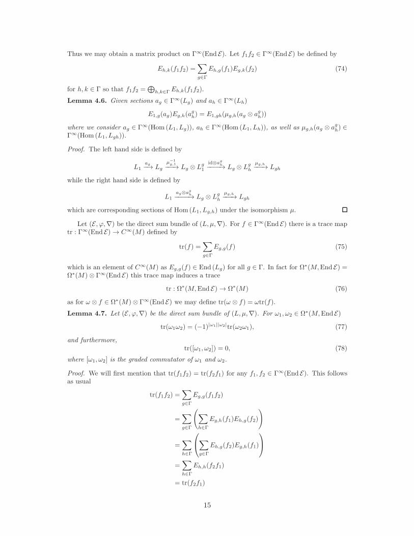
Thus we may obtain a matrix product on Γ∞(End E). Let f1f2 ∈ Γ∞(End E) be defined by

Eh,k(f1f2) =∑

g∈Γ

Eh,g(f1)Eg,k(f2) (74)

for h, k ∈ Γ so that f1f2 =⊕

h,k∈Γ Eh,k(f1f2).

Lemma 4.6. Given sections ag ∈ Γ∞(Lg) and ah ∈ Γ∞(Lh)

E1,g(ag)Eg,h(agh) = E1,gh(µg,h(ag ⊗ agh))

where we consider ag ∈ Γ∞(Hom (L1, Lg)), ah ∈ Γ∞(Hom (L1, Lh)), as well as µg,h(ag ⊗ agh) ∈Γ∞(Hom (L1, Lgh)).

Proof. The left hand side is defined by

L1ag

−→ Lg

µ−1g,1−−−→ Lg ⊗ Lg

1

id⊗ag

h−−−−→ Lg ⊗ Lgh

µg,h

−−−→ Lgh

while the right hand side is defined by

L1ag⊗ag

h−−−−→ Lg ⊗ Lgh

µg,h−−−→ Lgh

which are corresponding sections of Hom(L1, Lg,h) under the isomorphism µ.

Let (E , ϕ,∇) be the direct sum bundle of (L, µ,∇). For f ∈ Γ∞(End E) there is a trace maptr : Γ∞(End E)→ C∞(M) defined by

tr(f) =∑

g∈Γ

Eg,g(f) (75)

which is an element of C∞(M) as Eg,g(f) ∈ End (Lg) for all g ∈ Γ. In fact for Ω∗(M,End E) =Ω∗(M)⊗ Γ∞(End E) this trace map induces a trace

tr : Ω∗(M,End E)→ Ω∗(M) (76)

as for ω ⊗ f ∈ Ω∗(M)⊗ Γ∞(End E) we may define tr(ω ⊗ f) = ωtr(f).

Lemma 4.7. Let (E , ϕ,∇) be the direct sum bundle of (L, µ,∇). For ω1, ω2 ∈ Ω∗(M,EndE)

tr(ω1ω2) = (−1)|ω1||ω2|tr(ω2ω1), (77)

and furthermore,

tr([ω1, ω2]) = 0, (78)

where [ω1, ω2] is the graded commutator of ω1 and ω2.

Proof. We will first mention that tr(f1f2) = tr(f2f1) for any f1, f2 ∈ Γ∞(End E). This followsas usual

tr(f1f2) =∑

g∈Γ

Eg,g(f1f2)

=∑

g∈Γ

(∑

h∈Γ

Eg,h(f1)Eh,g(f2)

)

=∑

h∈Γ

∑

g∈Γ

Eh,g(f2)Eg,h(f1)

=∑

h∈Γ

Eh,h(f2f1)

= tr(f2f1)

15

by changing the summation order.Let ω1 = α1 ⊗ f1, ω2 = α2 ⊗ f2 where α1, α2 ∈ Ω∗(M) and f1, f2 ∈ Γ∞(End E). Then

|α1| = |ω1| and |α2| = |ω2| and

tr(ω1ω2) = tr((α1 ∧ α2)⊗ (f1f2))

= (α1 ∧ α2)tr((f1f2))

= (−1)|α1||α2|(α2 ∧ α1)tr((f2f1))

= (−1)|ω1||ω2|tr(ω2ω1)

From this it follows that

tr([ω1, ω2]) = tr(ω1ω2 − (−1)|ω1||ω2|ω2ω1) = tr(ω1ω2)− (−1)|ω1||ω2|tr(ω2ω1) = 0.

4.2 Derivations ∇k

We will again denote the discrepancy of (L, µ,∇) by α. For the rest of this section, fix thenotation (E , ϕ,∇E ) for the direct sum bundle of (L, µ,∇) as in Example 4.3.

Let pk : (M ⋊ Γ)(k) = M × Γk → M be defined by pk : (m, g1, . . . , gk) 7→ m ∈ M . Thepullback bundle Ek = p∗kE is a vector bundle over (M ⋊ Γ)(k). There is also a connection on Ekdefined by ∇Ek = p∗k∇

E . We will denote the connection ∇Ek |M×g1×···×gk by ∇Ek(g1, . . . , gk).Note with this definition that ∇Ek(g1, . . . , gk) = ∇

E for all g1, . . . , gk.

Remark 4.8. In general the collection πk : Ek → (M ⋊ Γ)(k) cannot be made into simplicialvector bundle using the maps (62) and (63). In order for the diagram (36) of face maps tocommute, we must have that δ∗i Ek−1

∼= Ek for 0 ≤ i ≤ k which does not hold in general.Specifically, consider δ∗0Ek−1. For any g1, . . . , gk ∈ Γ and m ∈M ,

δ∗0Ek−1(m, g1, . . . , gk) = δ∗0(p∗k−1E)(m, g1, . . . , gk)

= (p∗k−1E)(mg1, g2, . . . , gk)

= Eg1

∼= E ⊗ Lg−11

,

where the last isomorphism is given by ϕg−11

.

On the other hand, the vector bundles EndEk → (M ⋊ Γ)(k) do form a simplicial vectorbundle.

Proposition 4.9. The vector bundles πk : End Ek → (M⋊Γ)(k) form a simplicial vector bundle

π• : End E• → (M ⋊ Γ)•.

Proof. This follows as End (E ⊗Lg) ∼= End E . So δ∗i End Ek−1∼= EndEk and the diagram (36) of

face maps commutes for 0 ≤ i ≤ k.

Definition 4.10. Denote (M ⋊ Γ)∆(k) = (M ⋊ Γ)(k) × ∆k and E∆k = Ek × ∆k. Consider the

bundle πk × id : E∆k → (M ⋊ Γ)∆(k). Then define a connection

∇k : Γ∞(E∆k )→ Ω1((M ⋊ Γ)∆(k), E∆k ) (79)

by the formula

((∇k(g1, . . . , gk))s)(x1, . . . , xm, t1, . . . , tk)

= ((∇Ek(g1, . . . , gk) + t1A(g1) + · · ·+ tkA(g1 · · · gk))s)(x1, . . . , xm, t1, . . . , tk) (80)

16

where s ∈ Γ∞(E∆k ), x1, . . . , xm are coordinates on M (with m = dimM), and t1, . . . , tk areCartesian coordinates on ∆k.

Here we use ∇Ek to denote the derivation on E∆k → (M ⋊Γ)∆(k) that is the derivation ∇Ek on

Ek → (M ⋊ Γ)(k) at every point of ∆k. In other words, if pk : (M ⋊ Γ)∆(k) → (M ⋊ Γ)(k) is the

projection (x, t) 7→ x then we denote p∗k∇Ek merely by ∇Ek . Note that, while ∇k is a connection

on E∆k → (M ⋊ Γ)∆(k), ∇k is not a simplicial connection as Ek → (M ⋊ Γ)(k) does not form a

simplicial bundle.We may use the formal variable u to rescale the connection ∇k by considering (∇k)1,0 the

component of the operator ∇k

(∇k)1,0 : Γ∞(E∆k )→ Ω1((M ⋊ Γ)(k), Ek)⊗ C∞(∆k,∆k)

and (∇k)0,1 = d∆ the component that maps

(∇k)0,1 : Γ∞(E∆k )→ Γ∞(Ek)⊗ Ω1(∆k,∆k).

Let ∇ku = (∇k)1,0 + u−1d∆ so that

∇ku : Γ∞(E∆k )[u] // Ω1((M ⋊ Γ)∆(k), E

∆k )[u, u−1] (81)

We may extend ∇k to an operator

∇k : Ωℓ((M ⋊ Γ)∆(k), E∆k )→ Ωℓ+1((M ⋊ Γ)∆(k), E

∆k ) (82)

in the usual way. Given a section s ∈ Γ∞(E∆k ) and a form ω ∈ Ωℓ((M ⋊ Γ)∆(k)) we define

∇k(ω ⊗ s) = dω ⊗ s+ (−1)ℓω ∧ ∇ks. (83)

Remark 4.11. The operator ∇k may be defined to act on the algebra of End E-valued formsΩ∗(M,End E) and in particular sections Γ∞(End E) as follows. Given η ∈ Ω∗(M,End E), define

∇kη = [∇k, p∗kp∗kη] (84)

wherepk : (M ⋊ Γ)(k) →M (85)

is the projection (x, g1, . . . , gk) 7→ x,

pk : (M ⋊ Γ)(k) ×∆k → (M ⋊ Γ)(k) (86)

is the natural projection (x, t) 7→ x and we consider ∇k to be degree +1 with respect to thegraded commutator. In other words, ∇kη operates on sections s ∈ Γ∞(E∆k ) by

(∇kη)s = [∇k, p∗kp∗kη]s = ∇k((p∗kp

∗kη)s)− (−1)|η|+1(p∗kp

∗kη)(∇

ks). (87)

With this extension the rescaling ∇ku = (∇k)1,0 + u−1d∆ still makes sense.

Lemma 4.12. For any η ∈ Ω∗(M,End E),

(uddR + d∆)tr(η) = utr(∇ku(η)) (88)

where by tr(η) we mean tr(p∗kp∗kη).

Proof. We will omit the pullback maps p∗kp∗k as they should be clear from the context. As

∇ku = (∇k)1,0 + u−1d∆ and (∇k)1,0 = ddR + ω locally for some ω ∈ Ω1(M,End E). For a local

section s ∈ Γ∞(E∆k )

((∇k)1,0η)(s) = [(∇k)1,0, η]s

= [ddR + ω, η]s

= ddR(ηs)− (−1)|η|ηddRs+ [ω, η]s

= (ddRη + [ω, η])s

17

So by Lemma 4.7

tr((∇k)1,0η) = tr((ddRη + [ω, η]))

= tr(ddRη) + tr([ω, η])

= tr(ddRη)

= ddRtr(η).

Hence

utr(((∇k)1,0 + u−1d∆)η) = utr((∇k)1,0η) + tr(d∆η) = uddRtr(η) + d∆tr(η),

as required.

4.3 Simplicial 2-form

The collection of EndEk-valued 2-forms on (M ⋊Γ)(k)×∆k given by (∇k)2 for each k ≥ 0 does

not define a simplicial differential form on (M ⋊ Γ)•. In the theorem below we adjust (∇k)2 bya scalar-valued form to obtain a simplicial differential 2-form on M•.

Theorem 4.13. For each k ≥ 0, let ϑ(k) ∈ Ω2((M ⋊ Γ)∆(k),End E∆k ) be defined by the formula

ϑ(k)(g1, . . . , gk) = (∇k(g1, . . . , gk))2

−

k∑

i=1

tiθg1···gi −∑

1≤i<j≤k

α(g1 · · · gi, gi+1 · · · gj)(tidtj − tjdti). (89)

where α denotes the discrepancy of (L, µ,∇). Then ϑ = ϑ(k) is a compatible 2-form on

(M ⋊ Γ)• with values in End E•, which means that ϑ ∈ Ω2((M ⋊ Γ)•,End E•). We call ϑ the

simplicial 2-form associated to (L, µ,∇).

Proof. Our goal is to check the compatibility conditions of (11). First it will be helpful torewrite ϑ(k)(g1, . . . , gk). By expanding (∇k)2 using the definition of ∇k in (80),

(∇k(g1, . . . , gk))2 = (∇E )2 +

k∑

i=1

t2iA(g1 · · · gi)2 + [∇E , tiA(g1 · · · gi)]

+∑

1≤i<j≤k

[tiA(g1 · · · gi), tjA(g1 · · · gj)]

and by expanding [∇E , tiA(g1 · · · gi)] = dtiA(g1 · · · gi) + ti[∇E , A(g1 · · · gi)],

= θE +k∑

i=1

t2iA(g1 · · · gi)2 + dtiA(g1 · · · gi) + ti[∇

E , A(g1 · · · gi)]

+∑

1≤i<j≤k

[tiA(g1 · · · gi), tjA(g1 · · · gj)]

which, by substituting into (89), gives

ϑ(k)(g1, . . . , gk) = θE +k∑

i=1

t2iA(g1 · · · gi)2 + dtiA(g1 · · · gi) + ti[∇

E , A(g1 · · · gi)]− tiθg1···gi

+∑

1≤i<j≤k

[tiA(g1 · · · gi), tjA(g1 · · · gj)]− α(g1 · · · gi, gi+1 · · · gj)(tidtj − tjdti).

18

By adding and subtractingk∑

i=1

tiθE , factoring ti from some terms, and using t2i = ti− (1− ti)ti,

ϑ(k)(g1, . . . , gk) =

(1−

k∑

i=1

ti

)θE +

k∑

i=1

ti(θE +A(g1 · · · gi)

2 + [∇E , A(g1 · · · gi)]− θg1···gi)

+ dtiA(g1 · · · gi)− (1− ti)tiA(g1 · · · gi)2

+∑

1≤i<j≤k

[tiA(g1 · · · gi), tjA(g1 · · · gj)]− α(g1 · · · gi, gi+1 · · · gj)(tidtj − tjdti)

So by Equation (69) we have obtained

ϑ(k)(g1, . . . , gk)

=

(1−

k∑

i=1

ti

)θE +

k∑

i=1

tiϕ∗g1···giθ

Eg1···gi+ dtiA(g1 · · · gi)− (1− ti)tiA(g1 · · · gi)

2

+∑

1≤i<j≤k

[tiA(g1 · · · gi), tjA(g1 · · · gj)]− α(g1 · · · gi, gi+1 · · · gj)(tidtj − tjdti) (90)

As we are using Cartesian coordinates, when 1 ≤ ℓ ≤ k we have that

(id× ∂ℓ)∗ϑ(k)(g1, . . . , gk) = ϑ(k)(g1, . . . , gk)|tℓ=0 (91)

and when ℓ = 0 we have that

(id× ∂0)∗ϑ(k)(g1, . . . , gk) = ϑ(k)(g1, . . . , gk)|t1+···+tk=1 (92)

Therefore, to show that (id× ∂ℓ)∗ϑ(k) = (δℓ × id)∗ϑ(k−1) for 1 ≤ ℓ ≤ k − 1, we explicitly show

ϑ(k)(g1, . . . , gk)|tℓ=0 = ϑ(k−1)(g1, . . . , gℓgℓ+1, . . . , gk) (93)

Note that when tℓ = 0, dtℓ = 0. From the above

ϑ(k)(g1, . . . , gk)|tℓ=0 = θE +

k∑

i=1i6=ℓ

t2iA(g1 · · · gi)2 + [∇E , tiA(g1 · · · gi)]− tiθg1···gi

+∑

1≤i<j≤ki,j 6=ℓ

[tiA(g1 · · · gi), tjA(g1 · · · gj)]

− α(g1 · · · gi, gi+1 · · · gj)(tidtj − tjdti)

which may be written as ϑ(k−1)(g1, . . . , gℓgℓ+1, . . . , gk) upon reindexing ti+1 to ti when ℓ ≤i+ 1 ≤ k.

Now for the ℓ = 0 case, we explicitly show that

ϑ(k)(g1, . . . , gk)|t1+···+tk=1 = ϕ∗g1ϑ(k−1)(g2, . . . , gk)

g1 (94)

Note that when t1 + · · ·+ tk = 1 we have dt1 + · · ·+ dtk = 0. Before handling the ℓ = 0 case, itwill be helpful to do a couple side calculations.

Lemma 4.14. With the hypothesis of the theorem and assuming t1 + · · ·+ tk = 1,

∑

1≤i<j≤k

(tidtj − tjdti)α(g1 · · · gi, gi+1 · · · gj) =

k∑

j=2

dtjα(g1, g2 · · · gj)

+∑

2≤i<j≤k

(tidtj − tjdti)(α(g1, g2 · · · gi)− α(g1, g2 · · · gj) + α(g1 · · · gi, gi+1 · · · gj)) (95)

19

Proof. This is just a rearrangement of the summation:

∑

1≤i<j≤k

(tidtj − tjdti)α(g1 · · · gi, gi+1 · · · gj) =

=∑

2≤i<j≤k

(tidtj − tjdti)α(g1 · · · gi, gi+1 · · · gj)

+

k∑

j=2

(t1dtj − tjdt1)α(g1, g2 · · · gj)

=∑

2≤i<j≤k


+

k∑

j=2

((1−

k∑

ℓ=2

tℓ

)dtj − tj

(k∑

ℓ=2

(−dtℓ)

))α(g1, g2 · · · gj)

=∑

2≤i<j≤k


+

k∑

j,ℓ=2,j 6=ℓ

(tjdtℓ − tℓdtj)α(g1, g2 · · · gj) +

k∑

j=2

dtjα(g1, g2 · · · gj)

=

k∑

j=2

dtjα(g1, g2 · · · gj)

+∑

2≤i<j≤k

(tidtj − tjdti)(α(g1, g2 · · · gi)− α(g1, g2 · · · gj) + α(g1 · · · gi, gi+1 · · · gj))

Lemma 4.15. With the hypothesis of the theorem and assuming t1 + · · ·+ tk = 1,

∑

1≤i<j≤k

−titj(ϕ∗g1···giA(gi+1 · · · gj)

g1···gi)2

=

k∑

i=2

− (1− ti) ti(ϕ∗g1A(g2 · · · gi)

g1 )2 +∑

2≤i<j≤k

−titj [ϕ∗g1A(g2 · · · gi)

g1 , ϕ∗g1A(g2 · · · gj)

g1 ] (96)

Proof. We extract the i = 1 summands into a separate summation and rearrange

∑

1≤i<j≤k


g1···gi)2

=

k∑

j=2

− (1− t2 − · · · − tk) tj(ϕ∗g1A(g2 · · · gj)

g1 )2 +∑

2≤i<j≤k


g1···gi)2

=

k∑

j=2

− (1− tj) tj(ϕ∗g1A(g2 · · · gj)

g1 )2

+∑

2≤i<j≤k

−titj(ϕ∗g1···gi(A(gi+1 · · · gj)

g1···gi)2 − (ϕ∗g1A(g2 · · · gi)

g1)2 − (ϕ∗g1A(g2 · · · gj)

g1)2).

By adding and subtracting the same term in the second summation

=

k∑

j=2

− (1− tj) tj(ϕ∗g1A(g2 · · · gj)

g1 )2

20

+∑

2≤i<j≤k


g1···gi)2 − (ϕ∗g1A(g2 · · · gi)

g1)2 − (ϕ∗g1A(g2 · · · gj)

g1)2

+ [ϕ∗g1A(g2 · · · gi)

g1 , ϕ∗g1A(g2 · · · gj)

g1 ]− [ϕ∗g1A(g2 · · · gi)

g1 , ϕ∗g1A(g2 · · · gj)

g1 ])

we can rewrite the middle three terms in the second summation as a perfect square

=

k∑

i=2

− (1− ti) ti(ϕ∗g1A(g2 · · · gi)

g1 )2

+∑

2≤i<j≤k


g1···gi)2 − (ϕ∗g1A(g2 · · · gi)

g1 − ϕ∗g1A(g2 · · · gj)

g1)2

+ [ϕ∗g1A(g2 · · · gi)

g1 , ϕ∗g1A(g2 · · · gj)

g1 ])

and using Lemma 4.4 we have

=

k∑

i=2

− (1− ti) ti(ϕ∗g1A(g2 · · · gi)

g1 )2

+∑

2≤i<j≤k


g1···gi)2 − (α(g2 · · · gi, gi+1 · · · gj)− ϕ∗g1···giA(gi+1 · · · gj)

g1···gi)2

+[ϕ∗g1A(g2 · · · gi)

g1 , ϕ∗g1A(g2 · · · gj)

g1 ]).

Since α is a scalar-valued 1-form, the first two terms in the second summation cancel so that

=k∑

i=2

− (1− ti) ti(ϕ∗g1A(g2 · · · gi)

g1 )2 +∑

2≤i<j≤k

−titj[ϕ∗g1A(g2 · · · gi)

g1 , ϕ∗g1A(g2 · · · gj)

g1 ]

Now we will explicitly show that (id× ∂0)∗ϑ(k) = (δ0 × id)∗ϑ(k−1), i.e.

ϑ(k)(g1, . . . , gk)|t1+···+tk=1 = ϕ∗g1ϑ(k−1)(g2, . . . , gk)

g1 . (97)

Note that when t1 + · · · + tk = 1 we have dt1 + · · · + dtk = 0. We set t1 + · · · + tk = 1 in theexpression we obtained for ϑ(k)(g1, . . . , gk) in (90) to obtain

ϑ(g1, . . . , gk)|∑ki=1 ti=1 =

k∑

i=1

tiϕ∗g1···giθ

Eg1···gi+ dtiA(g1 · · · gi)−

k∑

j=1,j 6=i

tj

tiA(g1 · · · gi)

2

+∑

1≤i<j≤k

titj [A(g1 · · · gi), A(g1 · · · gj)]− (tidtj − tjdti)α(g1 · · · gi, gi+1 · · · gj). (98)

By rewriting

k∑

i=1

k∑

j=1,j 6=i

tj

tiA(g1 · · · gi)

2 =∑

1≤i<j≤k

titj(A(g1 · · · gi)

2 +A(g1 · · · gj)2),

we can factor the resulting terms appearing in the summation∑

1≤i≤j≤k

as a difference of squares

−A(g1 · · · gi)2 −A(g1 · · · gj)

2 + [A(g1 · · · gi), A(g1 · · · gj)] = − (A(g1 · · · gi)−A(g1 · · · gj))2.

21

Applying Lemma 4.4 this term equals

−(α(g1 · · · gi, gi+1 · · · gj)− ϕ∗

g1···giA(gi+1 · · · gj)g1···gi

)2

and because α is a scalar-valued 1-form this term simplifies to

(ϕ∗g1···giA(gi+1 · · · gj)

g1···gi)2

.

Hence

ϑ(g1, . . . , gk)|∑ki=1 ti=1 =

k∑

i=1

tiϕ∗g1···giθ

Eg1···gi+ dtiA(g1 · · · gi)

+∑

1≤i<j≤k


g1···gi)2− (tidtj − tjdti)α(g1 · · · gi, gi+1 · · · gj). (99)

Using Lemma 4.14 to rewrite the second term in the second summation as well as rewriting thesecond term in the first summation of (99) using dt1 + · · ·+ dtk = 0,

dtiA(g1 · · · gi) =

k∑

i=2

dti(A(g1 · · · gi)−A(g1)),

we obtain,

ϑ(g1, . . . , gk)|∑ki=1 ti=1 =

k∑

i=1

tiϕ∗g1···giθ

Eg1···gi+

k∑

i=2

dti(A(g1 · · · gi)−A(g1) + α(g1, g2 · · · gi))

+∑

1≤i<j≤k


g1···gi)2

−∑

2≤i<j≤k

(tidtj − tjdti)(α(g1, g2 · · · gi)− α(g1, g2 · · · gj) + α(g1 · · · gi, gi+1 · · · gj))

and by Lemma 4.4 and Corollary 4.5 we can simplify to

ϑ(g1, . . . , gk)|∑ki=1 ti=1 =

k∑

i=1

tiϕ∗g1···giθ

Eg1···gi−

k∑

i=2

dtiϕ∗g1A(g2 · · · gi)

g1

+∑

1≤i<j≤k


g1···gi)2−

∑

2≤i<j≤k

(tidtj−tjdti)ϕ∗g1α(g2 · · · gi, gi+1 · · · gj)

g1 .

Now focusing on the third summation of the previous expression, we apply Lemma 4.15 toobtain

ϑ(g1, . . . , gk)|∑ki=1 ti=1 =

k∑

i=1

tiϕ∗g1···giθ

Eg1···gi

+k∑

i=2

−dtiϕ∗g1A(g2 · · · gi)

g1 − (1− ti) ti(ϕ∗g1A(g2 · · · gi)

g1)2

−∑

2≤i<j≤k

titj [ϕ∗g1A(g2 · · · gi)

g1 , ϕ∗g1A(g2 · · · gj)

g1 ] + (tidtj − tjdti)ϕ∗g1α(g2 · · · gi, gi+1 · · · gj)

g1

22

Finally, as t1 = 1− t2 − · · · − tk, we rewrite first term of the first sum to obtain

ϑ(g1, . . . , gk)|∑ki=1 ti=1 = (1 − t2 − · · · − tk)ϕ

∗g1θ

Eg1+

k∑

i=2

tiϕ∗g1···giθ

Eg1···gi

+

k∑

i=2

−dtiϕ∗g1A(g2 · · · gi)

g1 − (1− ti) ti(ϕ∗g1A(g2 · · · gi)

g1)2

−∑

2≤i<j≤k

titj [ϕ∗g1A(g2 · · · gi)

g1 , ϕ∗g1A(g2 · · · gj)

g1 ] + (tidtj − tjdti)ϕ∗g1α(g2 · · · gi, gi+1 · · · gj)

g1

which is the form of ϕ∗g1ϑ(k−1)(g2, . . . , gk)

g1 that we obtained in (90) (with a relabeling ti → ti−1

for 2 ≤ i ≤ k), thus completing the calculation.

Remark 4.16. If we define ϑ′(k) by (∇k)2 = [ϑ′

(k), ·] then the discrepancy between ϑ′(k) and ϑ(k),

(ϑ′(k) − ϑ(k))(g1, . . . , gk) is given by

k∑

i=1

tiθg1···gi +∑

1≤i<j≤k

α(g1 · · · gi, gi+1 · · · gj)(tidtj − tjdti) (100)

which is a scalar-valued form. In other words, ϑ′(k)−ϑ(k) ∈ Ω2(M∆

(k)). Since a scalar valued form

in Ω2(M∆(k)) is central in Ω2(M∆

(k),EndE∆k ), [ϑ′

(k), ·] = [ϑ(k), ·]. Hence for any a ∈ Γ∞(End E∆k ),

(∇k)2(a) = [ϑ(k), a]. (101)

Definition 4.17. Notice from the previous formula for ϑ that ϑ0,2 = 0. We will then defineϑu = uϑ2,0 + ϑ1,1. With this rescaling we can view ϑu as an element of Ω0

−(M•)[u].

4.4 Simplicial curvature 3-form

Theorem 4.18. Let ϑ be the simplicial 2-form associated to (L, µ,∇) as in Theorem 4.13. Let

Θ(k) = −∇kϑ(k). The collection of 3-forms Θ(k) define a simplicial 3-form Θ = Θ(k) ∈

Ω3(M•). Furthermore, Θ0,3(k) = 0 as an element of Ωr,s(M•). The simplicial 3-form Θ =

−∇kϑ(k) is called the simplicial curvature 3-form associated to (L, µ,∇).

Proof. First let us provide a formula for Θ(k). Using the Bianchi identity

Θ(k)(g1, . . . , gk) =

= −(∇kϑ(k))(g1, . . . , gk)

= −(∇k)(g1, . . . , gk)

(∇k)2(g1, . . . , gk)−

k∑

i=1

tiθg1···gi −∑

1≤i<j≤k

α(g1 · · · gi, gi+1 · · · gj)(tidtj − tjdti)

= −(∇k)3(g1, . . . , gk) + (∇k(g1, . . . , gk))

k∑

i=1

tiθg1···gi +∑

1≤i<j≤k

α(g1 · · · gi, gi+1 · · · gj)(tidtj − tjdti)

=k∑

i=1

dtiθg1···gi +∑

1≤i<j≤k

dα(g1 · · · gi, gi+1 · · · gj)(tidtj − tjdti) + 2α(g1 · · · gi, gi+1 · · · gj)dtidtj ,

since θg and α(g, g′) are scalar-valued forms. Since there are no terms containing dti1dti2dti3where 1 ≤ i1, i2, i3 ≤ k, we explicitly see that Θ0,3

(k) = 0.

23

Using this formula, we can see Θ is a compatible form by a direct calculation. First we checkthat (id× ∂ℓ)

∗Θ(k) = (δℓ × id)∗Θ(k−1) for 1 ≤ ℓ ≤ k. Explicitly, when tℓ = 0 we have

Θ(k)(g1, . . . , gk)|tℓ=0 =

k∑

i=1i6=ℓ

dtiθg1···gi

+∑

1≤i<j≤ki,j 6=ℓ

dα(g1 · · · gi, gi+1 · · · gj)(tidtj − tjdti) + 2α(g1 · · · gi, gi+1 · · · gj)dtidtj

= Θ(k−1)(g1, . . . , gℓgℓ+1, . . . , gk)

by substituting ti for ti+1 whenever i > ℓ. Now when ℓ = 0, on the face t1 + · · · + tk = 1 wehave dt1 + · · ·+ dtk = 0 so that by replacing t1

Θ(k)(g1, . . . , gk)|t1+···+tk=1 =

k∑

i=2

dtiθg1···gi −

k∑

i=2

dtiθg1

+∑

2≤i<j≤k

dα(g1 · · · gi, gi+1 · · · gj)(tidtj − tjdti)

+

k∑

i=2

dα(g1, g2 · · · gi)((1 − t2 − · · · − tk)dti − ti(−dt2 − · · · − dtk))

+∑

2≤i<j≤k

2α(g1 · · · gi, gi+1 · · · gj)dtidtj +

k∑

i=2

2α(g1, g2 · · · gi)(−dt2 − · · · − dtk)dti

By Proposition 3.8 applied in the first two summations, Corollary 4.5, and dtidtj = −dtjdti,

=

k∑

i=2

dti(dα(g1, g2 · · · gi) + θg1g2···gi)

+∑

2≤i<j≤k

(dα(g1, g2 · · · gi)− dα(g1, g2 · · · gj) + dα(g1 · · · gi, gi+1 · · · gj))(tidtj − tjdti)

+

k∑

i=2

dα(g1, g2 · · · gi)dti +∑

2≤i<j≤k

2(α(g1, g2 · · · gi)− α(g1, g2 · · · gj) + α(g1 · · · gi, gi+1 · · · gj))dtidtj

=

k∑

i=2

dtiθg1g2···gi +

∑

2≤i<j≤k

dα(g2 · · · gi, gi+1 · · · gj)g1(tidtj − tjdti) + 2α(g2 · · · gi, gi+1 · · · gj)

g1dtidtj

= Θ(k−1)(g2, . . . , gk)g1

by a cancellation and application of Corollary 4.5 again.

Theorem 4.19. Let α be the discrepancy of (L, µ,∇), ϑ the associated simplicial 2-form, and

Θ the associated simplicial curvature 3-form. Then Θ ∈ Ω3(M•) is a representative of the

Dixmier-Douady class of (L, µ,∇).

Proof. We will apply the quasi-isomorphism of integration along simplices I∆ described inTheorem 2.13 to see I∆(Θ) = (α, θ) ∈ Ω1(M(2))⊕ Ω2(M(1)). For any g ∈ Γ,

Θ(1)(g) = dt1θg

24

so that restricted to M × g

I∆ : Θ(1)(g) 7→

∫

∆1

Θ(1)(g) =

∫ 1

0

θgdt1 = θg.

For any g1, g2 ∈ Γ,

Θ(2)(g1, g2) = dt1θg1dt2θg2 + dα(g1, g2)(t1dt2 − t2dt1) + 2α(g1, g2)dt1dt2

so that restricted to M × g1 × g2 we have

I∆ : Θ(2)(g1, g2) 7→

∫

∆2

Θ(2)(g1, g2)

=

∫

∆2

dt1θg1dt2θg2 + dα(g1, g2)(t1dt2 − t2dt1) + 2α(g1, g2)dt1dt2

=

∫

∆2

2α(g1, g2)dt1dt2

=

∫ 1

0

∫ 1−t1

0

2α(g1, g2)dt1dt2

= α(g1, g2).

Furthermore, Θr,s(k) = 0 for s ≥ 3, i.e. Θ(k) has at most two dt’s in any term, so that

I∆(Θ(k)) =

∫

∆k

Θ(k) = 0

whenever k ≥ 3. Hence I∆ : Θ 7→ α + θ so that Θ is a representative of the Dixmier-Douadyclass defined by (α, θ) in the bicomplex of compatible forms.

We may also introduce a rescaled version of the simplicial Dixmier-Douady form Θu in thecomplex Ω(M•)[u]

∗ as in (50). With the rescaling ∇ku = (∇k)1,0 + u−1d∆ we have ∇k

u(ϑu)(k) =u−1(Θu)(k) as

((∇k)1,0 + u−1d∆)(u(ϑ(k))2,0 + (ϑ(k))

1,1) = u((∇k)1,0(ϑ(k))2,0)3,0

+ ((∇k)1,0(ϑ(k))1,1 + d∆(ϑ(k))

2,0)2,1

+ u−1(d∆(ϑ(k)))1,2

= u(Θ(k))3,0 + (Θ(k))

2,1 + u−1(Θ(k))1,2

Also note that under this rescaling, u(∇ku)

2 = [(ϑu)(k), ·].

5 Cocycles on the twisted convolution algebra

Now we will prove the main theorem of this paper:

Theorem 5.1. Given a gerbe datum (L, µ,∇) on M ⋊ Γ, the map

Ψ2 Ψ1 Ψ0 τ∇ : (Ω((M ⋊ Γ)•)[u]•, dΘu

) // CC•(C∞c (M ⋊ Γ, L)[u−1, u], b+ uB) (102)

is a morphism from the twisted simplicial complex of M ⋊Γ to the (b, B) complex of the twisted

convolution algebra C∞c (M ⋊ Γ, L).

In Section 5.1 we define C∞c (M ⋊ Γ, L). The JLO morphism,

τ∇ : (Ω(M•)[u]•, dΘu


′),

is described in Section 5.2. The morphisms Ψ0, Ψ1, and Ψ2 are algebraic morphisms whichcompose to give a morphism

(C•(Γ, CC•(Γ∞c (EndE))[u−1, u]), b+ uB + δΓ

′) // CC•(C∞c (M ⋊ Γ, L)[u−1, u], b+ uB)

and are described in Section 5.3.

25

5.1 Twisted Convolution Algebra

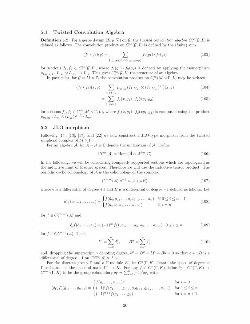
Definition 5.2. For a gerbe datum (L, µ,∇) on G, the twisted convolution algebra C∞c (G, L) is

defined as follows. The convolution product on C∞c (G, L) is defined by the (finite) sum

(f1 ∗ f2)(g) =∑

(g1,g2)∈G(2)|g1g2=g

f1(g1) · f2(g2) (103)

for sections f1, f2 ∈ C∞c (G, L), where f1(g1) · f2(g2) is defined by applying the isomorphism

µ(g1,g2) : L|g1 ⊗ L|g2∼−→ L|g. This gives C

∞c (G, L) the structure of an algebra.

In particular, for G = M ⋊ Γ, the convolution product on C∞c (M ⋊ Γ, L) may be written

(f1 ∗ f2)(x, g) =∑

g1g2=g

µg1,g2(f1|Mg1⊗ (f2|Mg2

)g1)(x, g) (104)

=∑

g1g2=g

f1(x, g1) · f2(xg1, g2) (105)

for sections f1, f2 ∈ C∞c (M × Γ, L), where f1(x, g1) · f2(xg1, g2) is computed using the product

µg1,g2 : Lg1 ⊗ (Lg2)g1 ∼−→ Lg.

5.2 JLO morphism

Following [15], [13], [17], and [22] we now construct a JLO-type morphism from the twistedsimplicial complex of M ⋊ Γ.

For an algebra A, let A = A⊕ C denote the unitization of A. Define

CCn(A) = Hom (A ⊗ A⊗n,C). (106)

In the following, we will be considering compactly supported sections which are topologized asthe inductive limit of Frechet spaces. Therefore we will use the inductive tensor product. Theperiodic cyclic cohomology of A is the cohomology of the complex

(CCn(A)[u−1, u], b+ uB), (107)

where b is a differential of degree +1 and B is a differential of degree −1 defined as follows. Let

dif(a0, a1, . . . , an) =

f(a0, a1, . . . , aiai+1, . . . , an) if 0 ≤ i ≤ n− 1

f(ana0, a1, . . . , an−1) if i = n(108)

for f ∈ CCn−1(A) and

sinf(a0, . . . , an) = (−1)nif(1, ai, . . . , an, a0, . . . , ai−1), 0 ≤ i ≤ n, (109)

for f ∈ CCn+1(A). Then

bn =

n∑

i=0

din, Bn =

n∑

i=0

sin, (110)

and, dropping the superscript n denoting degree, b2 = B2 = bB + Bb = 0 so that b + uB is adifferential of degree +1 on CCn(A)[u−1, u].

For the discrete group Γ and a Γ-module K, let Cn(Γ,K) denote the space of degree nΓ-cochains, i.e. the space of maps Γn → K. For any f ∈ Cn(Γ,K) define δΓ : Cn(Γ,K) →Cn+1(Γ,K) to be the group coboundary δΓ =

∑ni=0(−1)

iδΓi with

(δΓif)(g1, . . . , gn+1) =

f(g2, . . . , gn+1)g1 for i = 0

(−1)if(g1, . . . , gi−1, gigi+1, gi+2, . . . , gn+1) for 1 ≤ i ≤ n

(−1)n+1f(g1, . . . , gn) for i = n+ 1.

26

The superscript g1 denotes the action of g1 ∈ Γ on K. The cohomology of the complex(C•(Γ,K), δΓ) is group cohomology of Γ with coefficients in K. In particular we will considerthe complex

(Ck(Γ, CCn(Γ∞c (End E))[u−1, u]), (b+ uB) + (−1)nδΓ) (111)

of Γ-cochains with values in the periodic cyclic complex of Γ∞c (End E). By the operators b and

uB on such Γ-cochains we mean the operators defined by

(bf)(g1, . . . , gn) = b(f(g1, . . . , gn)) (112)

and(uBf)(g1, . . . , gn) = uB(f(g1, . . . , gn)) (113)

for any f ∈ Cn(Γ, CC•(Γ∞c (End E))[u−1, u]). Let us also denote δΓ

′ = (−1)nδΓ when δΓ is ofdegree n.

Lemma 5.3. For α(n) ⊗ β(n) ∈ Ω((M ⋊ Γ)(n))[u]0 ⊗ Ωn−1(∆n) we have the following

∫

M

∫

∆n

(uddR + d∆)(α(n) ⊗ β(n)) =

∫

M

α(n)

∫

∂(∆n)

β(n).

Also, for β(n) not of degree n−1 or α(n) not of degree 0 as elements of (Ω(M•)[u]∗)|(M⋊Γ)(n)×∆n

then the integral over M ×∆n is zero.

Proof. Note that α(n) ∈ Ω((M ⋊ Γ)(n))[u]0 must be a (dimM)-form on (M ⋊ Γ)(n). For any

g1, . . . , gn ∈ Γ denote α = α(n)(g1, . . . , gn). Then

∫

M

∫

∆n

(uddR + d∆)(α⊗ β(n)) =

∫

M

∫

∆n

(uddRα)⊗ β(n) +

∫

M

∫

∆n

α⊗ (d∆β(n))

=

∫

M

α

∫

∆n

dβ(n)

=

∫

M

α

∫

∂(∆n)

β(n)

by Stokes’ theorem.

Lemma 5.4. For any ω1 ∈ Ω((M ⋊ Γ)•)[u]∗ and ω2 ∈ Ω∗((M ⋊ Γ)•)[u]

∫

M

∫

∆n

((uddR + d∆)ω1) ∧ ω2 = −

∫

M

∫

∆n

ω1 ∧ ((uddR + d∆)ω2) + (−1)|ω2|

∫

M

∫

∂(∆n)

ω1 ∧ ω2

where ω2 is of fixed degree.

Proof. We have

∫

M

∫

∆n

((uddR + d∆)ω1) ∧ ω2

= −

∫

M

∫

∆n

ω1 ∧ ((uddR + d∆)ω2) + (−1)|ω2|

∫

M

∫

∆n

(uddR + d∆)(ω1 ∧ ω2)

= −

∫

M

∫

∆n

ω1 ∧ ((uddR + d∆)ω2) + (−1)|ω2|

∫

M

∫

∂(∆n)

ω1 ∧ ω2

where the first inequality follows from Lemma 2.20 and the second from Lemma 5.3.

27

Theorem 5.5. Given a gerbe datum (L, µ,∇) on M ⋊ Γ with associated simplicial 2-form ϑ,simplicial curvature 3-form Θ, and direct sum bundle E, there is a morphism

τ∇ : (Ω((M ⋊ Γ)•)[u]•, dΘu


′) (114)

defined by the JLO-type formula

τ∇(ω)(a0, a1, . . . , an)

=∑

k

∫

M

∫

∆k

ω(k)∧

(∫

∆n

tr(a0e−σ0(ϑu)(k)∇k

u(a1)e−σ1(ϑu)(k) · · · ∇k

u(an)e−σn(ϑu)(k))dσ1 · · · dσn

)

(115)

where ω = ω(k) ∈ Ω((M⋊Γ)•))[u]∗, a1, . . . , an ∈ Γ∞

c (End E), a0 ∈ ˜Γ∞c (EndE), and σ0, . . . , σn

are barycentric coordinates on ∆n.

Proof. Let us first discuss the reason the sum is finite. We must check in particular that thedegrees of the forms to be integrated on the simplices ∆k are bounded as k increases. Givenω ∈ Ω((M ⋊ Γ)•)[u]

ℓ, and a0, . . . , an ∈ Γ∞c (End E), consider

ω(k) ∧

(∫

∆n


u(a1)e−σ1(ϑu)(k) · · ·∇k

u(an)e−σn(ϑu)(k))dσ1 · · · dσn

)(116)

The maximum number of dti’s due to ω is ℓ, where ti are coordinates on the simplex ∆k,as the number of dti’s cannot exceed the degree of ω. Within the trace, the terms ∇k

u(ai)do not contribute any dti’s because aj is extended trivially to ∆n and (∇k)0,1 = d∆. Since

ϑ(k) = ϑ2,0(k) + ϑ1,1

(k) and in particular ϑ0,2(k) = 0, the contribution to the degree of the form from

all the (ϑu)(k) appearing must be at most dimM , i.e. the number of dxi’s, coordinates on themanifold M , is greater than or equal to the number of dtj ’s. Hence the simplex degree of theform above is at most ℓ+ dimM so the sum is finite.

Without loss of generality we will compute τ∇(dΘuω)(a0, a1, . . . , an) since

a0e−σ0(ϑu)(k)∇k

u(a1) · · · e−σn(ϑu)(k)

in the integrand above means

a0e−σ0(ϑu)(k)∇k

u(a1) · · · e−σn(ϑu)(k) + λe−σ0(ϑu)(k)∇k

u(a1) · · · e−σn(ϑu)(k)

for a0 = (a0, λ).Following [17], we will compute the effect of (uddR + d∆). This gives

τ∇((uddR + d∆)ω)(a0, a1, . . . , an)

=∑

k

∫

M

∫

∆k

(uddR + d∆)ω(k) ∧

(∫

∆n


u(a1) · · · e−σn(ϑu)(k))dσ1 · · · dσn

)

= −∑

k

∫

M

∫

∆k

ω(k) ∧

(∫

∆n

(uddR + d∆)tr(a0e−σ0(ϑu)(k)∇k

u(a1) · · · e−σn(ϑu)(k))dσ1 · · · dσn

)

+ (−1)n∫

M

∫

∂(∆k)

ω(k) ∧

(∫

∆n


u(a1) · · · e−σn(ϑu)(k))dσ1 · · · dσn

)

= −∑

k

∫

M

∫

∆k

ω(k) ∧

(∫

∆n

utr(∇ku(a0e

−σ0(ϑu)(k) · · · e−σn(ϑu)(k)))dσ1 · · · dσn

)(117)

+ (−1)n∫

M

∫

∂(∆k)

ω(k) ∧

(∫

∆n

tr(a0e−σ0(ϑu)(k) · · · e−σn(ϑu)(k))dσ1 · · · dσn

), (118)

28

where the second equality follows from Lemma 5.4, as the terms inside the trace ∇ku(ai) are of

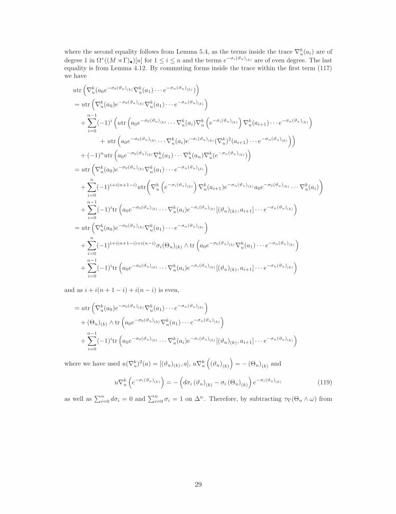
degree 1 in Ω∗((M ⋊Γ)•)[u] for 1 ≤ i ≤ n and the terms e−σi(ϑu)(k) are of even degree. The lastequality is from Lemma 4.12. By commuting forms inside the trace within the first term (117)we have

utr(∇k

u(a0e−σ0(ϑu)(k)∇k

u(a1) · · · e−σn(ϑu)(k))

)

= utr(∇k

u(a0)e−σ0(ϑu)(k)∇k

u(a1) · · · e−σn(ϑu)(k)

)

+

n−1∑

i=0

(−1)i(utr(a0e

−σ0(ϑu)(k) · · · ∇ku(ai)∇

ku

(e−σi(ϑu)(k)

)∇k

u(ai+1) · · · e−σn(ϑu)(k)

)

+ utr(a0e

−σ0(ϑu)(k) · · ·∇ku(ai)e

−σi(ϑu)(k)(∇ku)

2(ai+1) · · · e−σn(ϑu)(k)

))

+ (−1)nutr(a0e

−σ0(ϑu)(k)∇ku(a1) · · · ∇

ku(an)∇

ku(e

−σn(ϑu)(k)))

= utr(∇k


u(a1) · · · e−σn(ϑu)(k)

)

+

n∑

i=0

(−1)i+i(n+1−i)utr

(∇k

u

(e−σi(ϑu)(k)

)∇k

u(ai+1)e−σn(ϑu)(k)a0e

−σ0(ϑu)(k) · · · ∇ku(ai)

)

+

n−1∑

i=0

(−1)itr(a0e

−σ0(ϑu)(k) · · ·∇ku(ai)e

−σi(ϑu)(k) [(ϑu)(k), ai+1] · · · e−σn(ϑu)(k)

)

= utr(∇k


u(a1) · · · e−σn(ϑu)(k)

)

+

n∑

i=0

(−1)i+i(n+1−i)+i(n−i)σi(Θu)(k) ∧ tr(a0e

−σ0(ϑu)(k)∇ku(a1) · · · e

−σn(ϑu)(k)

)

+

n−1∑

i=0

(−1)itr(a0e

−σ0(ϑu)(k) · · ·∇ku(ai)e


)

and as i+ i(n+ 1− i) + i(n− i) is even,

= utr(∇k


u(a1) · · · e−σn(ϑu)(k)

)

+ (Θu)(k) ∧ tr(a0e

−σ0(ϑu)(k)∇ku(a1) · · · e

−σn(ϑu)(k)

)

+

n−1∑

i=0

(−1)itr(a0e

−σ0(ϑu)(k) · · ·∇ku(ai)e


)

where we have used u(∇ku)

2(a) = [(ϑu)(k), a], u∇ku

((ϑu)(k)

)= − (Θu)(k) and

u∇ku

(e−σi(ϑu)(k)

)= −

(dσi (ϑu)(k) − σi (Θu)(k)

)e−σi(ϑu)(k) (119)

as well as∑n

i=0 dσi = 0 and∑n

i=0 σi = 1 on ∆n. Therefore, by subtracting τ∇(Θu ∧ ω) from

29

τ∇((uddR + d∆)), we obtain a formula for τ∇(dΘuω)(a0, · · · , an)

−∑

k

∫

M

∫

∆k

ω(k) ∧

(∫

∆n

utr(∇ku(a0)e

−σ0(ϑu)(k) · · · e−σn(ϑu)(k))dσ1 · · · dσn

)(120)

−

∫

M

∫

∆k

ω(k) ∧

(∫

∆n

n−1∑

i=0

(−1)itr(a0e

−σ0(ϑu)(k) · · ·

· · ·∇ku(ai)e


))(121)

+ (−1)n∫

M

∫

∂(∆k)

ω(k) ∧

(∫

∆n

tr(a0e

−σ0(ϑu)(k)∇ku(a1) · · · e

−σn(ϑu)(k))dσ1 · · · dσn

)(122)

Next we compute the effect of the algebraic operators. The first term above, (120), is equivalentto −(uB)τ∇(ω)(a0, . . . , an) as

(uB)τ∇(ω)(a0, . . . , an)

=

n∑

i=0

(−1)niuτ∇(ω)(1, ai, . . . , an, a0, . . . ai−1)

=

n∑

i=0

(−1)niu∑

k

∫

M

∫

∆k

ω(k) ∧

(∫

∆n+1

tr(e−σ0(ϑu)(k)∇k

u(ai)e−σ1(ϑu)(k) · · ·

· · · ∇ku(an)e

−σn−i+1(ϑu)(k)∇ku(a0)e

−σn−i+2(ϑu)(k) · · · ∇ku(ai−1)e

−σn+1(ϑu)(k)

)dσ1 · · · dσn+1

)

=

n∑

i=0

(−1)niu∑

k

∫

M

∫

∆k

ω(k) ∧

(∫

∆n+1

tr(∇k

u(ai)e−σ1(ϑu)(k) · · ·

· · · ∇ku(an)e

−σn−i+1(ϑu)(k)∇ku(a0)e

−σn−i+2(ϑu)(k) · · · ∇ku(ai−1)e

−(σ0+σn+1)(ϑu)(k)

)dσ1 · · · dσn+1

)

=

n∑

i=0

(−1)ni+(n−i+1)iu∑

k

∫

M

∫

∆k

ω(k) ∧

(∫

∆n+1

tr(∇k

u(a0)e−σn−i+2(ϑu)(k) · · ·

· · · ∇ku(ai−1)e

−(σ0+σn+1)(ϑu)(k)∇ku(ai)e

−σ1(ϑu)(k) · · · ∇ku(an)e

−σn−i+1(ϑu)(k)

)dσ1 · · · dσn+1

)

=

n∑

i=0

u∑

k

∫

M

∫

∆k

ω(k) ∧

(∫

∆n

σitr(∇k


u(a1) · · ·

· · · ∇ku(an)e

−σn(ϑu)(k)

)dσ1 · · · dσn

)

= u∑

k

∫

M

∫

∆k

ω(k) ∧

(∫

∆n

tr(∇k


u(a1) · · · ∇ku(an)e

−σn(ϑu)(k)

)dσ1 · · · dσn

)

where we have changed variables, performed a partial integration, and then used that∑

σi = 1.The second term in τ∇(dΘu

ω)(a0, . . . , an), (121), is −bτ∇(ω)(a0, . . . , an) as

bτ∇(ω)(a0, . . . , an)

=

n−1∑

i=0

(−1)iτ∇(a0, . . . , aiai+1, . . . , an) + (−1)nτ∇(ana0, a1, . . . , an−1)

=∑

k

∫

M

∫

∆k

ω(k) ∧

(∫

∆n−1

tr(∇k

u(a0a1)e−σ0(ϑu)(k)∇k

u(a2) · · ·

· · · ∇ku(an)e

−σn−1(ϑu)(k)

)dσ1 · · · dσn−1

)

30

+

n−1∑

i=1

(−1)i∑

k

∫

M

∫

∆k

ω(k) ∧(∫

∆n−1

(tr(a0e

−σ0(ϑu)(k)∇ku(a1) · · ·

· · · e−σi−1(ϑu)(k)∇ku(aiai+1)e

−σi(ϑu)(k) · · · ∇ku(an)e

−σn−1(ϑu)(k))dσ1 · · · dσn−1

)

+ (−1)n∑

k

∫

M

∫

∆k

ω(k) ∧(∫

∆n−1

tr(∇k

u(ana0)e−σ0(ϑu)(k)∇k

u(a1) · · ·

· · · ∇ku(an−1)e

−σn−1(ϑu)(k))dσ1 · · · dσn−1

)

and because ∇ku(aiai+1) = ∇

ku(ai)ai+1 + ai∇

k(ai+1) we have

=∑

k

∫

M

∫

∆k

ω(k) ∧(∫

∆n−1

tr(∇k

u(a0)a1e−σ0(ϑu)(k)∇k

u(a2) · · ·

· · · ∇ku(an)e

−σn−1(ϑu)(k))dσ1 · · · dσn−1

)

+∑

k

∫

M

∫

∆k

ω(k) ∧(∫

∆n−1

tr(a0∇

ku(a1)e

−σ0(ϑu)(k)∇ku(a2) · · ·

· · · ∇ku(an)e

−σn−1(ϑu)(k))dσ1 · · · dσn−1

)

+n−1∑

i=1

(−1)i∑

k

∫

M

∫

∆k

ω(k) ∧(∫

∆n−1

tr(a0e

−σ0(ϑu)(k)∇ku(a1) · · ·

· · · e−σi−1(ϑu)(k)∇ku(ai)ai+1e


−σn−1(ϑu)(k))dσ1 · · · dσn−1

)

+

n−1∑

i=1

(−1)i∑

k

∫

M

∫

∆k

ω(k) ∧(∫

∆n−1

tr(a0e

−σ0(ϑu)(k)∇ku(a1) · · ·

· · · e−σi−1(ϑu)(k)ai∇ku(ai+1)e


−σn−1(ϑu)(k))dσ1 · · · dσn−1

)

+ (−1)n∑

k

∫

M

∫

∆k

ω(k) ∧(∫

∆n−1

tr(∇k

u(an)a0e−σ0(ϑu)(k)∇k

u(a1) · · ·

· · · ∇ku(an−1)e

−σn−1(ϑu)(k))dσ1 · · · dσn−1

)

+ (−1)n∑

k

∫

M

∫

∆k

ω(k) ∧(∫

∆n−1

tr(an∇

ku(a0)e

−σ0(ϑu)(k)∇ku(a1) · · ·

· · · ∇ku(an−1)e

−σn−1(ϑu)(k))dσ1 · · · dσn−1

)

and by combining terms as well as commuting terms in the trace of the last two terms

=

n∑

i=1

(−1)i−1∑

k

∫

M

∫

∆k

ω(k) ∧(∫

∆n−1

tr(a0e

−σ0(ϑu)(k)∇ku(a1) · · ·

· · · e−σi−2(ϑu)(k)∇ku(ai−1)[ai, e

−σi−1(ϑu)(k) ]∇ku(ai+1) · · ·

· · · ∇ku(an)e

−σn−1(ϑu)(k))dσ1 · · · dσn−1

)

As [ai, ·] is a derivation, we can use the integration formula of [21], Equation 7.2, to obtain

[ai, e−σi(ϑu)(k) ] =

∫ 1

0

e−(1−σ)σi(ϑu)(k) [ai,−σi (ϑu)(k)]e−σσi(ϑu)(k)dσ

= σi

∫ 1

0

e−(1−σ)σi(ϑu)(k) [(ϑu)(k) , ai]e−σσi(ϑu)(k)dσ

31

so that we have

=

n∑

i=1

(−1)i−1∑

k

∫

M

∫

∆k

ω(k) ∧

(∫

∆n−1

∫ 1

0

σitr(a0e−σ0(ϑu)(k)∇k

u(a1) · · ·

· · · e−σi−2(ϑu)(k)∇ku(ai−1)e

−(1−σ)σi(ϑu)(k) [(ϑu)(k) , ai]e−σσi(ϑu)(k)∇k

u(ai+1) · · ·

· · · ∇ku(an)e

−σn−1(ϑu)(k))dσdσ1 · · · dσn−1

)

Now by the change of variables in the i-th term, (1 − σ)σi = σ′i−1 and σ′

i = σi−1σ (as well asσ0 = σ′

0, . . . , σi−2 = σ′i−2 and σi = σ′

i+1, . . . , σn−1 = σ′n) we have σi−1 = σ′

i−1 + σ′i, and in fact

σ′0 + · · · + σ′

n = 1 and dσ′0 + · · · + dσ′

n = 0, i.e. barycentric coordinates on ∆n. So with thischange of variables the above expression is equivalent to (121).

The third term in τ∇(dΘuω), (122), equals δΓ

′τ∇(ω)(a0, . . . , an) because ϑ(k) and ω(k)

are simplicial forms. In particular, if we define Cartesian coordinates on ∆k by t1, . . . , tk thenthe restriction of ϑ(k) to the face ti = 0 is a form on ∆k−1 given by

ϑ(k)(g1, . . . , gk)|ti=0 = ϑ(k−1)(g1, . . . , gigi+1, . . . , gk)

for 1 ≤ i ≤ k − 1 andϑ(k)(g1, . . . , gk)|tk=0 = ϑ(k−1)(g1, . . . , gk−1)

The restriction to the face∑k

i=1 ti = 1 is a form on ∆k−1 given by

ϑ(k)(g1, . . . , gk)|∑

ti=1 = ϑ(k−1)(g2, . . . , gk)g1

as shown in Theorem 4.13. Hence the corresponding identities hold for ϑu. We also have thesame sort of identities for ω(k) because ω(k) is a simplicial form. In addition ∇k(g1, . . . , gk)satisfies the following identities for 1 ≤ i ≤ k − 1

∇k(g1, . . . , gk)|ti=0 = ∇E + t1A(g1) + · · ·+ ti−1A(g1 · · · gi−1) + ti+1A(g1 · · · gi+1) + · · ·

· · ·+ tkA(g1 · · · gk)

= ∇k−1(g1, . . . , gigi+1, . . . , gk)

with a change of variables. Similarly ∇k(g1, . . . , gk)|tk=0 = ∇k−1(g1, . . . , gk−1). Furthermore,

∇k(g1, . . . , gk)|∑ ti=1 = ∇E +A(g1) + t2(A(g1g2)−A(g1)) + · · ·+ tk(A(g1 · · · gk)−A(g1))

= ϕ∗g1(∇

Eg

⊗ 1 + 1⊗∇g) + t2(α(g1, g2) + ϕ∗g1A(g2)

g1 ) + · · ·

· · ·+ tk(α(g1, g2 · · · gk) + ϕ∗g1A(g2 · · · gk))

= ϕ∗g1(∇

Eg

+ t2A(g2) + · · ·+ tkA(g2 · · · gk))g1

+ ϕ∗g1∇g + t2α(g1, g2) + · · · tkα(g1, g2 · · · gk)

= ϕ∗g1(∇

Eg

+ t2A(g2) + · · ·+ tkA(g2 · · · gk))g1

∼= ∇k−1(g2, . . . , gk)g1

by Lemma 4.4 and the definition of A(g1). Since ∇g + t2α(g1, g2) + · · · tkα(g1, g2 · · · gk) isscalar-valued,

[∇k−1(g2, . . . , gk)g1 + ϕ∗

g1∇g + t2α(g1, g2) + · · · tkα(g1, g2 · · · gk), η] = [∇k−1(g2, . . . , gk)g1 , η]

for any η ∈ C∞c (M,End E). The corresponding identities hold for ∇k

u as well.Taking orientation into account we may write

∂(∆k) = ∆k|∑ ti=1 −∆k|t1=0 +∆k|t2=0 · · ·+ (−1)k+1∆k|tk=0

32

where a negative sign denotes the orientation opposite the orientation induced by ∆k. Withthis the third term of τ∇(dΘu

ω)(a0, . . . , an), (122), may be written

(−1)n∑

k

∫

M

∫

∆k|∑ ti=1

ω(k) ∧

(∫

∆n


u(a1) · · · e−σn(ϑu)(k))dσ1 · · · dσn

)

+ (−1)nk∑

i=1

(−1)i∫

M

∫

∆k|ti=0

ω(k) ∧

(∫

∆n

tr(a0e−σ0(ϑu)(k) · · · e−σn(ϑu)(k))dσ1 · · · dσn

).

And evaluation on g1, . . . , gk gives

(−1)n∑

k

∫

M

∫

∆k−1

ω(k−1)(g2, . . . , gk)g1 ∧

(∫

∆n

tr(a0e−σ0((ϑu)(k−1)(g2,...,gk))

g1

(∇k−1u (g2, . . . , gk)(a1))

g1 · · · e−σn((ϑu)(k−1)(g2,...,gk))g1

)dσ1 · · · dσn

)

+ (−1)nk−1∑

i=1

(−1)i∫

M

∫

∆k−1

ω(k−1)(g1, . . . , gigi+1, . . . , gk)∧

∧

(∫

∆n

tr(a0e−σ0(ϑu)(k−1)(g1,...,gigi+1,...,gk)(∇k−1

u (g1, . . . , gigi+1, . . . , gk))(a1) · · ·

· · · e−σn(ϑu)(k−1)(g1,...,gigi+1,...,gk))dσ1 · · · dσn

)

+ (−1)n(−1)k∫

M

∫

∆k−1

ω(k−1)(g1, . . . , gk−1)∧

∧

(∫

∆n

tr(a0e−σ0(ϑu)(k−1)(g1,...,gk−1)(∇k−1

u (g1, . . . , gk−1))(a1) · · ·

· · · e−σn(ϑu)(k−1)(g1,...,gk−1))dσ1 · · · dσn

)

= (−1)nτ∇(ω)(g2, . . . , gk)g1(a0, . . . , an)

+ (−1)nk−1∑

i=1

τ∇(ω)(g1, . . . , gigi+1, . . . , gk)(a0, . . . , an)

+ (−1)n(−1)kτ∇(ω)(g1, . . . , gk−1)(a0, . . . , an)

= δΓ′τ∇(ω)(g1, . . . , gk)(a0, . . . , an)

This proves that τ∇ dΘu= (−(b+ uB) + δΓ

′) τ∇.

5.3 Algebraic morphisms

Now we will need a different cochain complex computing group cohomology. For a discretegroup Γ and a Γ-module K, let Cn(Γ,K) denote the space of homogenous n-cochains of Γ with

values in K. This is the space of degree n + 1 Γ-cochains, i.e. the space of maps Γn+1 → K,that satisfy the condition

gf(g0, . . . , gn) = f(gg0, . . . , ggn).

For any f ∈ Cn(Γ,K) define δΓ : Cn(Γ,K) // Cn+1(Γ,K) by

(δΓf)(g0, . . . , gn) =

n∑

i=0

(−1)if(g0, . . . , gi, . . . , gn) (123)

and let δ′Γ = (−1)nδΓ. There is a bijection from Cn(Γ,K) // Cn(Γ,K) given by f 7→ f where

f is defined by

f(g0, . . . , gn) = f(g−10 g1, (g0g1)

−1g2, . . . , (g0 · · · gn−1)−1gn) (124)

33

for any f ∈ Cn(Γ,K) and g0, . . . , gn ∈ Γ. The complex (C(Γ,K), δΓ) also computes groupcohomology.

Proposition 5.6. The above bijection induces a map

Ψ0 : (C•(Γ, CC•(Γ∞c (End E))[u−1, u]), b+ uB + δΓ

′)

// (C•(Γ, CC•(Γ∞c (End E))[u−1, u]), b+ uB + δ′Γ) (125)

by the formula

Ψ0(c)(g0, . . . , gn) = c(g−10 g1, (g0g1)

−1g2, . . . , (g0 · · · gn−1)−1gn) (126)

for any c ∈ C•(Γ, CC•(Γ∞c (End E))[u−1, u]).

Lemma 5.7. There is a contracting homotopy

h : (Ck(Γ, CCn(Γ∞c (End E))[u−1, u]), δΓ, (−1)

k(b+ uB))

// (Ck−1(Γ, CCn(Γ∞c (End E))[u−1, u]), δΓ, (−1)

k(b+ uB))

Proof. First we will define a map γ : Γ∞c (End E)⊗n // CΓ by

γ : Eg0,g1(a0)⊗ Eg1,g2(a1)⊗ . . .⊗ Egn,g0(an) 7→ g0 (127)

where Egi,gi+1(ai), Egn,g0(an) ∈ Γ∞c (End E) for 0 ≤ i ≤ n− 1. Note that by multilinearity,

γ(Eg0,g1(a0) + Eg′

0,g1(a′0), Eg1,g2(a1), . . . , Egn,g0(an) + Egn,g′

0(a′n)) = g0 + g′0. (128)

Furthermore, the map γ is equivariant:

γ(g · (Eg0,g1(a0)⊗ . . .⊗ Egn,g0(an))) = γ(Egg0,gg1(ag0)⊗ . . .⊗ Eggn,gg0(a

gn))

= gg0

= gγ(Eg0,g1(a0)⊗ . . .⊗ Egn,g0(an))

Then we can define a map

h : Ck+1(Γ, CCn(Γ∞c (End E))) // Ck(Γ, CCn(Γ∞

c (EndE))) (129)

by(hϕ)(g0, . . . , gk)(s) = (−1)kϕ(g0, . . . , gk, γ(s))(s) (130)

for any s ∈ Γ∞c (End E)⊗n.

The map h is a contracting homotopy for group cochains as we have

(δΓh)f(g0, . . . , gk)(s) =

k∑

i=0

(−1)i(hf)(g0, . . . , gi, . . . , gk)(s)

= (−1)k−1k∑

i=0

(−1)if(g0, . . . , gi, . . . , gk, γ(s))(s)

(hδΓ)f(g0, . . . , gk)(s) = (−1)k(δΓf)(g0, . . . , gk, γ(s))(s)

= (−1)kk∑

i=0

(−1)if(g0, . . . , gi, . . . , gk, γ(s))(s)

+ (−1)k+(k+1)f(g0, . . . , gk)(s)

so that(δΓh+ hδΓ) = 1 (131)

is the identity operator.

34

Theorem 5.8. Given a gerbe datum (L, µ,∇) on M ⋊Γ and an (L, µ,∇)-twisted vector bundle

with connection (E , ϕ,∇E ), there is a morphism

Ψ1 : (C•(Γ, CC•(Γ∞c (End E))[u−1, u]), b+ uB + δ′Γ) // (CC•(Γ∞

c (End E))[u−1, u], b+ uB)Γ

from the complex of cochains on Γ taking values in the periodic cyclic complex of Γ∞c (End E) to

the periodic cyclic complex of Γ-invariant cochains on Γ∞c (End E).

Proof. Now we will view

(C•(Γ, CC•(Γ∞c (End E))[u−1, u]), b+ uB + δ′Γ)

as a bicomplex(Ck(Γ, CCn(Γ∞

c (End E))[u−1, u]), δΓ, (−1)k(b + uB))

with horizontal differential δΓ and vertical differential b + uB. More explicitly this is done viaa morphism

Ψ1/2 : (C•(Γ, CC•(Γ∞c (End E))[u−1, u]), b+ uB + δ′Γ)

// (Ck(Γ, CCn(Γ∞c (End E))[u−1, u]), δΓ, (−1)

k(b+ uB))

which is defined by exchanging the vertical and horizontal differentials and making the appro-priate sign adjustments δ′Γ 7→ δΓ and (b+ uB) 7→ (−1)k(b+ uB).

Since the map h is a contracting homotopy for the rows of this bicomplex, i.e. the rows ofthe augmented double complex are exact, the cohomology of the bicomplex is the cohomologyof the initial column. As described in [2] in the case of the Cech-de Rham complex, an explicitmorphism

Ψk1 : (Ck(Γ, CCn(Γ∞

c (End E))[u−1, u]), δΓ, (−1)k(b + uB))

// (CCn+k(Γ∞c (End E))[u−1, u], b+ uB)Γ

is given by the formula

Ψk1(c) = (−(b+ uB)h)kc− h(−(b+ uB)h)k−1((b+ uB)c)− h(−(b+ uB)h)k(δΓc).

For cochains in column k denote D = (−1)k(b+ uB) for the sake of brevity. Then this formulais

Ψk1(c) = (−Dh)kc− h(−Dh)k−1(Dc)− h(−Dh)k(δΓc).

Then let Ψ1 =∑

k Ψk. We will also denote Ψ1Ψ1/2 merely by Ψ1, as in the theorem statement.

We can see immediately that if c is a group k-cochain then

Ψ1(c) ∈ C0(Γ, CCn+k(Γ∞c (EndE))[u−1, u])

because

(Dh) : Ci(Γ, CCj(Γ∞c (End E))[u−1, u]) // Ci−1(Γ, CCj+1(Γ∞

c (End E))[u−1, u]).

At this point let us recount a lemma from [2].

Lemma 5.9. For i ≥ 1δΓ(Dh)i = (Dh)iδΓ − (Dh)i−1D

Proof of lemma. Since δΓ anticommutes with D and δΓh+ hδΓ = 1,

δΓ(Dh)(Dh)i−1 = −DδΓh(Dh)i−1

= −D(1− hδΓ)(Dh)i−1

= (Dh)δΓ(Dh)i−1

35

Therefore we can commute δΓ and (Dh) until we reach (Dh)i−1δΓ(Dh). We obtain the formulaby

δΓ(Dh)(Dh)i−1 = (Dh)i−1δΓ(Dh)

= −(Dh)i−1D(1− hδΓ)

= −(Dh)i−1D + (Dh)iδΓ

The first step in proving Ψ1 is a morphism is to check that Ψ1(c) does in fact land in thecomplex of Γ-invariant cyclic cochains CCn+k(Γ∞

c (End E)[u−1, u], b + uB)Γ. To check this we

compute δΓΨ1(α). By the above lemma

δΓΨk1(c) = δΓ(−Dh)kc− δΓh(−Dh)k−1Dc− δΓh(−Dh)k δΓc

= (−Dh)kδΓc+ (−Dh)k−1Dc− δΓh(−Dh)k−1Dc− δΓh(−Dh)k δΓc

= (1− δΓh)(−Dh)k δΓc+ (1 − δΓh)(−Dh)k−1Dc

= (1− δΓh)(−Dh)k−1(−DhδΓ +D)c

= (1− δΓh)(−Dh)k−1(D(1− hδΓ))c

= (hδΓ)(−Dh)k−1(DδΓh)c

and by applying the lemma again

= h((−Dh)k−1δΓ + (−Dh)k−2D)(DδΓh)c

= h((−Dh)k−1δΓ(DδΓh)c+ h(−Dh)k−2D)(DδΓh)c

= 0

by D2 = 0 and (δΓ)2 = 0 as well as commuting D and δΓ. The cases δΓΨ

11(c) = 0 and

δΓΨ01(c) = 0 are straightforward. Since δΓΨ1(c) = 0 we see that Ψ1(c) is Γ-invariant.Further, the boundary operators commute with Ψ1. For any c ∈ Ck(Γ, CCn(Γ∞

c (End E))[u−1, u])

Ψ1((δΓ +D)c) = Ψk1(Dc) + Ψk+1

1 (δΓc)

= (−Dh)k(Dc)− h(−Dh)k−1D(Dc)− h(−Dh)kδΓ(Dc)

+ (−Dh)k+1(δΓc)− h(−Dh)kD(δΓc)− h(−Dh)k+1δΓ(δΓc)

which, by the commutation relations for the boundary operators,

= (−Dh)kDc+ (−Dh)k+1δΓc

= −Dh(−Dh)k−1Dc−Dh(−Dh)k δΓc

= D((−Dh)kc− h(−Dh)k−1Dc− h(−Dh)kδΓc)

= DΨk1(c) = DΨ1(c)

Hence Ψ1 is a morphism.

Theorem 5.10. Given a gerbe datum (L, µ,∇) on M⋊Γ with an (L, µ,∇)-twisted vector bundle

(E , ϕ,∇E ), there is a morphism

Ψ2 : CC•(Γ∞c (End E)[u−1, u], b+ uB)Γ // CC•(C∞

c (M ⋊ Γ, L)[u−1, u], b+ uB) (132)

36

defined by the formula

Ψ2(c)(ag0 , . . . , agn) = c(E1,g0 (ag0), . . . , Eg0···gi−1,g0···gi(ag0···gi−1gi ), . . . , Eg0···gn−1,1(a

g0···gn−1gn ))

(133)for any g0, . . . gn ∈ Γ. Here c is a cochain in CCn(Γ∞

c (EndE))Γ and agi is a section in Γ∞c (Lgi)

for 0 ≤ i ≤ n, and ag0 = (ag0 , λ) for λ ∈ C.

Proof. Note that E1,g0(ag0) = ˜E1,g0(ag0) in ˜Γ∞c (End E). Since a ∈ C∞

c (M ⋊ Γ, L) may bewritten a =

∑g∈Γ ag where ag ∈ Γ∞

c (Lg) for g ∈ Γ, it is sufficient to define Ψ2 on such sections.Also note that (ag ∗ ag′) ∈ Γ∞

c (Lgg′) since

(ag ∗ ag′)(x, h) =∑

h1h2=h

ag(x, h1) · ag′(xh1, h2)

= ag(x, g) · ag′(xg, g′)

= µg,g′(ag ⊗ agg′)(x, gg′).

As the coboundary bn =∑n

i=1 din, we will prove that d

iΨ2 = Ψ2di for 1 ≤ i ≤ n. For 1 ≤ i ≤ n,

(diΨ2)(c)(ag0 , . . . , agn+1)

= Ψ2(c)(ag0 , . . . , agi ∗ agi+1 , . . . , agn+1)

= Ψ2(c)(ag0 , . . . , µgi,gi+1(agi ⊗ agigi+1

), . . . , agn+1

)

= c(E1,g0(ag0), . . . , Eg0···gi−1,g0···gi+1((µgi,gi+1(agi ⊗ agigi+1

))g0···gi−1), . . . , Eg0···gn,1(ag0···gngn+1

))

= c(E1,g0(ag0), . . . , Eg0···gi−1,g0···gi+1(µ

g0···gi−1gi,gi+1

(ag0···gi−1gi ⊗ ag0···gigi+1

)), . . . , Eg0···gn,1(ag0···gngn+1

))

= c(E1,g0(ag0), . . . , Eg0···gi−1,g0···gi(a

g0···gi−1gi )Eg0···gi,g0···gi+1(a

g0···gigi+1

), . . . , Eg0···gn,1(ag0···gngn+1

))

= (dic)(E1,g0(ag0), . . . , Eg0···gi−1,g0···gi(a

g0···gi−1gi ), Eg0···gi,g0···gi+1(a

g0···gigi+1

), . . . , Eg0···gn,1(ag0···gngn+1

))

= (Ψ2di)(c)(ag0 , . . . , agn+1).

For the case of d0Ψ2 = Ψ2d0 note that ag0 ∗ ag1 = ag0 ∗ ag1 + λag1

(d0Ψ2)(c)(ag0 , . . . , agn+1)

= Ψ2(c)(ag0 ∗ ag1 , ag2 , . . . , agn+1)

= Ψ2(c)(ag0 ∗ ag1 + λag1 , ag2 , . . . , agn+1)

= Ψ2(c)(ag0 ∗ ag1 , ag2 , . . . , agn+1) + Ψ2(c)(λag1 , ag2 , . . . , agn+1)

= Ψ2(c)(µg0,g1(ag0 ⊗ ag0g1), ag2 , . . . , agn+1) + Ψ2(c)(λag1 , ag2 , . . . , agn+1)

= c(E1,g0g1(µg0,g1(ag0 ⊗ ag0g1)), Eg0g1,g0g1g2(ag0g1g2 ), . . . , Eg0...gn,1(a

g0···gngn+1

))

+ c(λE1,g1(ag1 ), Eg1,g1g2(ag1g2), . . . , Eg1···gn,g

−10

(ag1···gngn+1))

= c(E1,g0g1(µg0,g1(ag0 ⊗ ag0g1), Eg0g1,g0g1g2(ag0g1g2 ), . . . , Eg0...gn,1(a

g0···gngn+1

))

+ c(λE1,g1(ag1 ), Eg1,g1g2(ag1g2), . . . , Eg1···gn,1(a

g1···gngn+1

)) · g0

= c(E1,g0g1(µg0,g1(ag0 ⊗ ag0g1), Eg0g1,g0g1g2(ag0g1g2 ), . . . , Eg0...gn,1(a

g0···gngn+1

))

+ c(λEg0,g0g1(ag0g1), Eg0g1,g0g1g2(a

g0g1g2 ), . . . , Eg0g1···gn,g0(a

g0···gngn+1

))

as the second term is nonzero only if g0 · · · gn+1 = 1 and g1 · · · gn+1 = 1, i.e. g0 = 1

= c(E1,g0(ag0)Eg0,g0g1(a

g0g1), Eg0g1,g0g1g2(a

g0g1g2 ), . . . , Eg0···gn,1(a

g0···gngn+1

))

+ c(λEg0,g0g1(a


g0g1g2 ), . . . , Eg0···gn,1(a

g0···gngn+1

))

37


g0g1) + λEg0,g0g1(a


g0g1g2 ), . . . , Eg0···gn,1(a

g0···gngn+1

))



g0g1g2 ), . . . , Eg0···gn,1(a

g0···gngn+1

))

= (d0c)(E1,g0(ag0), Eg0,g0g1(a

g1g0), . . . , Eg0···gn,1(a

g0···gngn+1

))

= (Ψ2d0)(c)(ag0 , . . . , agn+1)

We also have dn+1Ψ2 = Ψ2dn+1 as

(dn+1Ψ2)(c)(ag0 , . . . , agn+1)

= Ψ2(c)(agn+1 ∗ ag0 , . . . , agn)

= c(E1,gn+1g0(µ(agn+1 ⊗ agn+1g0 )), Egn+1g0,gn+1g0g1(a

gn+1g0g1 ), . . . , Egn+1g0···gn−1,1(a

gn+1g0···gn−1gn ))

= c(E1,gn+1g0(µ(agn+1 ⊗ agn+1g0 )), Egn+1g0,gn+1g0g1(a

gn+1g0g1 ), . . . , Egn+1g0···gn−1,1(a

gn+1g0···gn−1gn )) · g−1

n+1

= c(Eg0···gn,g0(µ(agn+1 ⊗ agn+1g0 )), Eg0,g0g1(a

g0g1), . . . , Eg0···gn−1,g0···gn(a

g0···gn−1gn ))

= c(Eg0···gn,1(agn+1)E1,g0(agn+1g0 ), Eg0,g0g1(a

g0g1), . . . , Eg0···gn−1,g0···gn(a

g0···gn−1gn ))

= (dn+1c)(E1,g0(agn+1g0 )), Eg0,g0g1(a

g0g1), . . . , Eg0···gn,1(a

g0···gngn+1

))

= (Ψ2dn+1)(c)(ag0 , . . . , agn+1)

and the extension to ag0 = (ag0 , λ) is not much different from the previous calculation. Thisshows that bΨ2 = Ψ2b.

Next we show that BΨ2 = Ψ2B. As B =∑

i si we will show that siΨ2 = Ψ2s

i for 0 ≤ i ≤ n.The identity element in C∞

c (M ⋊ Γ, L) is (0, 1) where 0 may be considered as the sum of zerosections 0 : M → Lg for any g, so we consider 0 as 0 : M → L1 below.

(Ψ2si)(c)(ag0 , . . . , agn)

= (sic)(E1,g0(ag0), . . . , Eg0···gi−1,g0···gi(a

g0···gi−1gi ), . . . , Eg0···gn−1,1(a

g0···gn−1gn )

)

= (sic)(E1,g0(ag0), . . . , Eg0···gi−1,g0···gi(a

g0···gi−1gi ), . . . , Eg0···gn−1,1(a

g0···gn−1gn )

)· (gi · · · gn)

= (sic)(Egi···gn,gi···gng0(a

gi···gng0 ), . . . , Egi···gng0···gi−2,1(a

gi···gng0···gi−2gi−1

),

E1,gi(agi), . . . , Egi···gn−1,gi···gn(agi···gn−1gn )

)

= c(1, E1,gi(agi), Egi,gigi+1(a

gigi+1

), . . . , Egi···gn−1,gi···gn(agi···gngn ),

Egi···gn,gi···gng0(agi···gng0 ), . . . , Egi···gng0···gi−2,1(a

gi···gng0···gi−2gi−1

))

= (Ψ2c)(1, agi , . . . , agn , ag0 , . . . , agi)

= (siΨ2)(c)(ag0 , . . . , agn).

Hence Ψ2 is a morphism.

This completes the proof of the main theorem, Theorem 5.1.

References

[1] Raoul Bott. On characteristic classes in the framework of Gelfand-Fuchs cohomology.Asterisque, (32-33):113–139, 1976.

[2] Raoul Bott and Loring Tu. Differential Forms in Algebraic Topology. Springer, New York,1982.

[3] Peter Bouwknegt, Alan L. Carey, Varghese Mathai, Michael K. Murray, and Danny Steven-son. Twisted K-theory and K-theory of bundle gerbes. Communications in Mathematical

Physics, 228(1):17–49, 2002.

38

[4] Paul Bressler, Alexander Gorokhovsky, Ryszard Nest, and Boris Tsygan. Deformations ofgerbes on smooth manifolds. In K-Theory and Noncommutative Geometry, EMS Series ofCongress Reports, pages 349–393. European Mathematical Society, 2008.

[5] Jean-Luc Brylinski. Loop Spaces, Characteristic Classes, and Geometric Quantization.Birkhauser, Boston-Basel-Berlin, 1993.

[6] Alan L. Carey, Jouko Mickellson, and Michael K. Murray. Bundle gerbes applied to quan-tum field theory. Reviews in Mathematical Physics, 12(1):65–90, 2000.

[7] Alain Connes. Noncommutative Geometry. Academic Press, 1994.

[8] Marius Crainic. Cyclic Cohomology of Etale Groupoids; The General Case. K-Theory, 17,1999.

[9] Johan L. Dupont. Curvature and characteristic classes. Number 640 in Lecture Notes inMathematics. Springer-Verlag, Berlin-Heidelberg-New York, 1978.

[10] Marcello Felisatti and Frank Neumann. Secondary theories for simplicial manifolds andclassifying spaces. Geometry & Topology Monographs, 11:33–58, 2007.

[11] Krzysztof Gawedzki and Nuno Reis. WZW branes and gerbes. Reviews in Mathematical

Physics, 14(12):1281–1334, 2002.

[12] Jean Giraud. Cohomologie non abelliene. Number 179 in Die Grundlehren der mathema-tischen Wissenschaften. Springer-Verlag, Berlin-New York, 1971.

[13] Alexander Gorokhovsky. Characters of cycles, equivariant characteristic classes, and Fred-holm modules. Communications in Mathematical Physics, 208(1):1–23, 1999.

[14] Nigel Hitchin. Lectures on special Lagrangian submanifolds. In Cumrun Vafa and S.-T.Yau, editors, Winter School on Mirror Symmetry, Vector Bundles and Lagrangian Sub-

manifolds, number 23 in Studies in Advanced Mathematics, pages 151–182, Providence,2001. AMS/International Press.

[15] Arthur Jaffe, Andrzej Lesniewski, and Konrad Osterwalder. Quantum K-theory, I. Cherncharacter. Communications in Mathematical Physics, 118(1):1–14, 1988.

[16] Jean-Louis Loday. Cyclic Homology. Number 301 in Die Grundlehren der mathematischenWissenschaften. Springer-Verlag, Berlin-Heidelberg-New York, 2nd edition, 1998.

[17] Varghese Mathai and Danny Stevenson. On a generalised Connes-Hochschild-Kostant-Rosenberg theorem. Advances in Mathematics, 200(2):303–335, 2006.

[18] Varghese Mathai and Danny Stevenson. Entire cyclic homology of stable continuous tracealgebras. Bulletin of the London Mathematical Society, 39(1):71–75, 2007.

[19] Ieke Moerdijk. Orbifolds as Groupoids: an Introduction. In Alejandro Adem, Jack Morava,and Youngbim Ruan, editors, Orbifolds in Mathematics and Physics, number 310 in Con-temporary Mathematics, pages 205–222, Providence, 2002. AMS.

[20] Ieke Moerdijk and Janez Mrcun. Introduction to Foliations and Lie Groupoids. CambridgeUnivesity Press, Cambridge, UK, 2003.

[21] Dan Quillen. Algebra cochains and cyclic cohomology. Publ. Math. IHES, 68:139–174,1989.

[22] Jean-Louis Tu and Ping Xu. Chern character for twisted K-theory of orbifolds. Advancesin Mathematics, 207(2):455–483, 2006.

39

Cyclic cocycles on twisted convolution algebras

Documents

Transcript of Cyclic cocycles on twisted convolution algebras