The Prediction of the Performance of a Twisted Rudder - MDPI

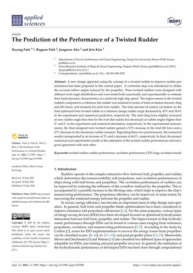
applied sciences

Article

The Prediction of the Performance of a Twisted Rudder

Ilryong Park 1,*, Bugeun Paik 2, Jongwoo Ahn 2 and Jein Kim 1

��

Citation: Park, I.; Paik, B.; Ahn, J.;

Kim, J. The Prediction of the

Performance of a Twisted Rudder.

Appl. Sci. 2021, 11, 7098. https://

doi.org/10.3390/app11157098

Academic Editor: Maria Grazia

De Giorgi

Received: 15 July 2021

Accepted: 30 July 2021

Published: 31 July 2021

Publisher’s Note: MDPI stays neutral

with regard to jurisdictional claims in

published maps and institutional affil-

iations.

Copyright: © 2021 by the authors.

Licensee MDPI, Basel, Switzerland.

This article is an open access article

distributed under the terms and

conditions of the Creative Commons

Attribution (CC BY) license (https://

creativecommons.org/licenses/by/

4.0/).

1 Department of Naval Architecture and Ocean Engineering, Dong-Eui University, Busan 47340, Korea;[email protected]

2 Korea Research Institute of Ships & Ocean Engineering, Daejeon 34103, Korea; [email protected] (B.P.);[email protected] (J.A.)

* Correspondence: [email protected]; Tel.: +82-051-890-2595

Abstract: A new design approach using the concept of a twisted rudder to improve rudder per-formances has been proposed in the current paper. A correction step was introduced to obtainthe accurate inflow angles induced by the propeller. Three twisted rudders were designed withdifferent twist angle distributions and were tested both numerically and experimentally to estimatetheir hydrodynamic characteristics at a relatively high ship speed. The improvement in the twistedrudders compared to a reference flat rudder was assessed in terms of total cavitation amount, dragand lift forces, and moment for each twin rudder. The total amount of surface cavitation on thefinal optimized twin twisted rudder at a reference design rudder angle decreased by 43% and 34.4%in the experiment and numerical prediction, respectively. The total drag force slightly increasedat zero rudder angle than that for the twin flat rudder but decreased at rudder angles higher than4◦ and 6◦ in the experiment and numerical simulation, respectively. In the experimental measure-ments, the final designed twin twisted rudder gained a 5.5% increase in the total lift force and a37% decrease in the maximum rudder moment. Regarding these two performances, the numericalresults corresponded to an increase of 3% and a decrease of 66.5%, respectively. In final, the presentnumerical and experimental results of the estimation of the twisted rudder performances showed agood agreement with each other.

Keywords: twisted rudder; rudder performance; cavitation performance; CFD; large cavitation tunnel

1. Introduction

Rudders operate in the complex interactive flow between hull, propeller, and rudder,which determines the maneuverability, self-propulsion, and cavitation performances ofships along with hull forms and propellers. The cavitation performance of rudders canbe improved by reducing the influence of the crossflow induced by the propeller. This isaccompanied by a possible increase in the lift-drag ratio, which helps to improve the ship’smaneuvering performance. The propulsion efficiency can be improved, to some extent, byrecovering the rotational energy between the propeller and rudder.

In recent, energy efficiency has become an important issue in ship design and oper-ation. In general, hull form and propeller blade optimizations have been considered toimprove resistance and propulsion efficiencies [1,2]. For the same purposes, various typesof energy-saving devices (ESDs) have been developed focused on optimized hydrodynamicinteraction between hull form, propeller, and rudder. The improvement of ship hydrody-namic performance through ESDs can be found in various cases ranging from resistance,propulsion, cavitation, and maneuvering performances [2–7]. According to the study byCarlton [2], zones for ESD implementations to recover the energy losses from propellerscan be classified as pre- [8–10], in- [11–13], and post-propeller plane [14,15]. Meanwhile,Mewis and Deichmann [8] and Watson [14] also classified two different types of approachesadoptable for ESDs: pre-rotating and post propeller recovery. In general, the estimation ofthe hydrodynamic performance of developed ESDs has been done through computational

Appl. Sci. 2021, 11, 7098. https://doi.org/10.3390/app11157098 https://www.mdpi.com/journal/applsci

https://www.mdpi.com/journal/applsci

https://www.mdpi.com

https://doi.org/10.3390/app11157098


https://creativecommons.org/

https://creativecommons.org/licenses/by/4.0/

https://creativecommons.org/licenses/by/4.0/


https://www.mdpi.com/journal/applsci

https://www.mdpi.com/article/10.3390/app11157098?type=check_update&version=1

Appl. Sci. 2021, 11, 7098 2 of 24

fluid dynamics (CFD) simulations and/or model tests performed in a towing tank anda cavitation tunnel. It is reported that discrepancies have been found between CFD andITTC 1978 prediction concerning the scale effects on ESDs’ performances estimated atmodel scale [16], and the need for CFD simulations at full-scale conditions and sea trialsto assess these scale effects has been discussed [17]. There is limited sea trial data in thepublic domain, but it is clear that several ESDs have been fitted to operational ships andattempted in full-scale trials [18].

Shen et al. [18] investigated the scale effects on ships with ESDs using CFD simulationsand reported the reliability of CFD data at full scale compared to model scale. Moriet al. [19], Ohtagaki et al. [20], and Okamoto et al. [21] studied a rudder bulb, or anadditional device in a fin on the rudder bulb to retrieve the energy loss behind the propeller.These studies showed that rudder bulbs devised increase propulsion efficiency by reducinghub drag, which is caused by decreased separation and pressure pulse. Liu et al. [22]showed the energy-saving effect of the combination of rudder bulb and rudder thrust finis better than that of rudder bulb at full-scale trials. Kanemaru et al. [23] proposed twokinds of newly developed rudders that obtain the low drag effectively comparing withthe conventional rudder. Chen et al. [24] employed a parametric geometry design usingthe non-uniform rational B-splines (NURBS) technique to obtain the best rudder geometryfor improving propulsive efficiency, where rudder optimization was performed based onCFD. Rhee et al. [25] developed rudder gap flow-blocking devices to suppress rudder gapcavitation and carried out cavitation observation and pressure measurement in a cavitationtunnel for the estimation of their cavitation performances. Paik et al. [26] investigated theunsteady cavity patterns around the gap of the conventional and newly developed semi-spade rudders for marine ships using a high-speed CCD camera, time-resolved particleimage velocimetry (PIV) analysis, and pressure measurements. The relationship betweenthe cavitation phenomenon on the rudder surface and the rudder angles was analyzedby Paik et al. [27], where PIV technology was adopted to observe the flow field betweenpropeller and rudder. Reichel [28] carried out an experimental investigation of the effectof rudder location on the propulsion efficiency of a single-screw, single-rudder containership. Krasilnikov et al. [29] experimentally analyzed the hydrodynamic characteristics ofthe propeller-rudder system at low-speed operation.

The problem of rudder cavitation has been an issue due to the type of rudder thathas been adopted to most large ships [30]. Thus, full-spade rudders have been used forhigh-speed vessels and researched to avoid cavitation problems. Nishiyama [31] providedan empirical formula of inflow angle for twisted rudder generation and discussed theeffectiveness of reaction rudder on rudder cavitation. Shen et al. [32] proposed a rudderdesign method to improve rudder cavitation performance and tested a twisted rudder ina large cavitation channel concerning rudder surface cavitation and cavitation inceptionspeed. Kim et al. [33] and Choi et al. [34] developed twisted full-spade rudders basedon incoming flow angles for a large container ship to recover the swirl energy for thepropeller slipstream. Kim et al. [35] designed three twisted rudders for a large containercarrier and verified the speed performances of the ship improved by those twisted ruddersthrough model tests in a towing. Furthermore, they analyzed the change in self-propulsionfactors by the twisted rudders. Ahn et al. [36] developed a twisted rudder to overcomethe cavitation problems of large container carriers in the way of the leading edge alsoconsidering manufacturing productivity. They called this rudder the X-Twisted rudder andverified its hydrodynamic performances through various model tests such as resistance,self-propulsion, cavitation, and maneuvering tests. Sun et al. [37] performed numericalsimulations and cavitation tunnel experiments to predict the hydrodynamic performanceof twisted rudders and verify the energy-saving effect. Kim et al. [38] designed a twistedrudder by using the genetic algorithm and investigated cavitation behaviors on the ruddersurface. A wavy twisted rudder superior to a conventional full-spade twisted rudder withregard to lift-drag ratio and stall delay was proposed and verified by Shin et al. [39].

Appl. Sci. 2021, 11, 7098 3 of 24

In general, most research on twisted rudders has been carried out for single-screwships. However, this study focused on a twin twisted rudder of a surface combatantand investigated its effects on hydrodynamic performances. In the current work, a noveldesign of a twisted rudder has been proposed to improve the rudder performance of anexisting surface combatant. Our approach involved prediction and correction of twist angledistribution which compensate for the effect of inflow angles induced by the propeller.While developing the design of the twisted rudder, our main focus was to improve therudder cavitation performance without any loss of lift performance. The primary designcriteria are a decrease in rudder moment and a decrease in the drag force of the twistedrudder up to a certain level which is not harmful to the ship’s self-propulsion performance.Three twisted rudders with three different twist angle distributions were designed usingthe results of the CFD simulations and tested both numerically and experimentally toestimate their hydrodynamic performances at a relatively high ship speed. Using the sametest setup and procedures, a reference flat rudder was also tested to validate the effectof twist angles on the rudder performance. The numerical and experimental evaluationsmainly focused on the rudder surface cavitation, rudder forces, and moment. The initialtwist angle distribution was predicted from numerical simulation and its accuracy wasestimated. A method of correction of the predicted initial inflow angles induced by thepropeller was proposed and applied to obtain the final corrected distribution of twist angles.An intermediate distribution of the twist angles between the initial and final corrected twistangles was produced to see the variation effect of the twist angle on rudder hydrodynamicperformances. In the current paper, the improvement of the twisted rudders comparedwith the reference flat rudder is discussed in terms of total cavitation amount, drag, lift,and moment for each twin rudder.

2. Experimental Approaches

Model tests to analyze the hydrodynamic performance of twisted rudders including areference flat rudder were carried out in the large cavitation tunnel (LCT) at the KRISO.The main dimensions of the LCT in the length (L), width (W), and height (H) directionsare 60 m × 6.5 m × 19.8 m. The test section where the ship model was installed hasdimensions of 12.5 m (L) × 2.8 m (W) × 1.8 m (H). Figure 1a,b show an experimental setupfor the current test ship model with full appendages in the LCT test section. The shiphull form is a surface combatant, and its model size has a length of 7.07 m, a breadth of0.933 m, and a draft of 0.269 m as shown in Table 1. The propeller is a controllable pitchpropeller (CPP) with five blades and rotates outboard. The propeller model diameter (DP)is 0.28 m. As shown in Table 1, the flat rudder has the section profiles of symmetricalNACA sections at the root and the tip. As will be explained in detail later, three twistedrudders were made by rotating each cross-section of the flat rudder around the mid-chordpoint according to the predicted inflow angle distributions. The chord length (c) of therudder model is 0.1967 m at the root and 0.0887 m at the tip. The span length (s) is 0.2147 m.The sign of the rudder angle, δR, was defined as positive when rotating in the directionof the starboard side. Figure 1c shows the holes on the inboard and outboard surfaces ofthe flat rudder to measure the pressure distributions along the two-chord lines at the spanlocations, z/s = 0.45 and 0.6. This pressure measurement was carried out at 18-knot shipspeed and non-cavitating flow conditions. Fourteen pressure taps were installed alongthe rudder surface at 60% span of the rudder. The relative pressure was measured withthe pressure transducers made by Validyne DP15. The pressure was measured with anuncertainty of 0.18%. The pressure was non-dimensionalized as follows:

Cp =p− po12 ρwU2

o(1)

where, p is the pressure, po is the free stream reference pressure, ρw is the water densityand Uo is the inflow velocity in the LCT test section. The hydrodynamic performances ofthe flat and twisted rudders were estimated by the surface cavitation, the drag and lift

Appl. Sci. 2021, 11, 7098 4 of 24

forces, and the moment for each rudder. For this purpose, the model tests were performedfor cavitating flows at a relatively high ship speed, Vs = 30 knots. The correspondingtest conditions are shown in Table 2. Here, KT is the thrust coefficient, n is the propellerrotational speed, σn,0.5RP is the cavitation number at the radial position of 0.5RP and RPis the propeller radius. The thrust coefficient KT and the cavitation number σn,0.5RP aregiven as:

KT =T

ρwn2D4P

(2)

σn,0.5R =pT − pv

0.5ρwn2D2P

(3)

where, T is the thrust of the propeller, pT is the static pressure in the LCT and pv is thevapor pressure. The rudder forces and moment were measured by using a dynamometer. Adynamometer was installed in the stern hull over the rudder to measure the drag force (D)in the x-direction, the lift force (L) in the y-direction, and the moment (M) in the z-directionacting on the rudder. The dynamometer was manufactured by Wonbang Forcetech Co. Ltd.,Daejeon, Korea, and can measure drag, lift, and moment up to 1000 N, 2000 N, and 45 Nm,respectively with uncertainties of 0.38%, 0.23%, and 1.70%. The drag, lift, and momentcoefficients are defined as follows:

CD =D

12 ρwU2

o S(4)

CL =L

12 ρwU2

o S(5)

CM =M

12 ρwU2

o S`c(6)

where, S is the lateral projected area of the rudder and `c is the moment arm from the ruddercentroid to the rotation axis in the chord direction. Surface cavitation on each rudder wasrecorded through a charge-coupled device (CCD) video camera with the accompanyinglightening system.

Table 1. Main dimensions of the ship, propeller and rudder models.

Ship

Length between perpendiculars 7.067 m

Breath 0.933 m

Draft 0.269 m

Propeller

Propeller Diameter 0.28 m

Number of blades 5

Rotation Direction Outward

Rudder

Root chord length 0.1967 m

Tip chord length 0.0887 m

Span length 0.2147 m

Table 2. LCT test conditions for cavitating flow.

Vs KT σn,0.5R Uo n

30.0 kts 0.1879 1.2485 9.0 m/s 31.61 rps

Appl. Sci. 2021, 11, 7098 5 of 24

Appl. Sci. 2021, 11, x FOR PEER REVIEW 4 of 24

where, is the pressure, is the free stream reference pressure, is the water density and is the inflow velocity in the LCT test section. The hydrodynamic performances of the flat and twisted rudders were estimated by the surface cavitation, the drag and lift forces, and the moment for each rudder. For this purpose, the model tests were performed for cavitating flows at a relatively high ship speed, = 30 knots. The corresponding test conditions are shown in Table 2. Here, is the thrust coefficient, n is the propeller rota-tional speed, , . is the cavitation number at the radial position of 0.5 and is the propeller radius. The thrust coefficient and the cavitation number , . are given as: = (2)

, . = . (3)

where, T is the thrust of the propeller, is the static pressure in the LCT and is the vapor pressure. The rudder forces and moment were measured by using a dynamometer. A dynamometer was installed in the stern hull over the rudder to measure the drag force ( ) in the x-direction, the lift force (ℒ) in the y-direction, and the moment (ℳ) in the z-direction acting on the rudder. The dynamometer was manufactured by Wonbang Force-tech Co. Ltd., Daejeon, Korea, and can measure drag, lift, and moment up to 1000 N, 2000 N, and 45 Nm, respectively with uncertainties of 0.38%, 0.23%, and 1.70%. The drag, lift, and moment coefficients are defined as follows: = 12 (4)

= ℒ12 (5)

= ℳ12 ℓ (6)

where, is the lateral projected area of the rudder and ℓ is the moment arm from the rudder centroid to the rotation axis in the chord direction. Surface cavitation on each rud-der was recorded through a charge-coupled device (CCD) video camera with the accom-panying lightening system.

(a) (b)


(c)

Figure 1. Experimental setup in the LCT: (a) full appended ship model mounted in the test section; (b) close-up view of the stern region; (c) pressure measurement holes on the inboard and outboard surfaces of the port flat rudder.

Table 1. Main dimensions of the ship, propeller and rudder models.

Ship Length between perpendiculars 7.067 m

Breath 0.933 m Draft 0.269 m

Propeller Propeller Diameter 0.28 m Number of blades 5 Rotation Direction Outward

Rudder Root chord length 0.1967 m Tip chord length 0.0887 m

Span length 0.2147 m

Table 2. LCT test conditions for cavitating flow

, . n 30.0 kts 0.1879 1.2485 9.0 m/s 31.61 rps

3. Numerical Approaches 3.1. Reynolds-Averaged Navier-Stokes Equations

The RANS equations with turbulence models were solved to simulate wetted and cavitating flows around the test ship model, since the RANS models have been shown to be still successful in the estimation of the hydrodynamic performances of ships and off-shore structures. A single set of the mass conservation and RANS momentum conserva-tion equations in Cartesian coordinates for two-phase (vapor and liquid) incompressible flows is given by: = 0 (7)

∂ ρ + = − + + − (8)

where, is the fluid density, are the time-averaged velocity components correspond-ing to the Cartesian coordinates , is time, are the velocity fluctuations, is the time-averaged pressure, is the fluid dynamic viscosity and − are the Reynolds stresses. The Reynolds stress term can be defined in terms of known quantities. In turbu-lence modeling, the problem is to develop a suitable closure model to predict the Reynolds stresses. As one of the various types of turbulence closure models, the Boussinesq hypoth-esis provides a simple relationship between the Reynolds stresses and velocity gradients through the eddy viscosity as follows: − = + (9)

Figure 1. Experimental setup in the LCT: (a) full appended ship model mounted in the test section; (b) close-up view of thestern region; (c) pressure measurement holes on the inboard and outboard surfaces of the port flat rudder.

3. Numerical Approaches3.1. Reynolds-Averaged Navier-Stokes Equations

The RANS equations with turbulence models were solved to simulate wetted andcavitating flows around the test ship model, since the RANS models have been shown to bestill successful in the estimation of the hydrodynamic performances of ships and offshorestructures. A single set of the mass conservation and RANS momentum conservationequations in Cartesian coordinates for two-phase (vapor and liquid) incompressible flowsis given by:

∂Ui∂xj

= 0 (7)

∂(ρUi)

∂t+ Uj

∂(ρUi)

∂xj= − ∂P

∂xj+

∂

∂xj

(µ

∂Ui∂xj

)+

∂(−ρu′iu

′j

)∂xj

(8)

where, ρ is the fluid density, Ui are the time-averaged velocity components corresponding tothe Cartesian coordinates xi, t is time, u′i are the velocity fluctuations, P is the time-averagedpressure, µ is the fluid dynamic viscosity and −ρuiuj are the Reynolds stresses. TheReynolds stress term can be defined in terms of known quantities. In turbulence modeling,the problem is to develop a suitable closure model to predict the Reynolds stresses. As oneof the various types of turbulence closure models, the Boussinesq hypothesis provides asimple relationship between the Reynolds stresses and velocity gradients through the eddyviscosity µt as follows:

− ρuiuj = µt

(∂Ui∂xj

+∂Uj

∂xi

)(9)

Among the two-equation turbulence models, the realizable k − ε model based onthe suggestions by Shih et al. [40] was used. This model uses the transport equationsfor the turbulent kinetic energy k and turbulence dissipation rate as the standard k − εmodel. Better predictions of the distribution of the dissipation rate and boundary layer

Appl. Sci. 2021, 11, 7098 6 of 24

characteristics in a large pressure gradient, separated, and recirculating flows can beexpected compared to the standard k − εmodel.

3.2. Cavitation Model

A mixture approach was used to solve the cavitating flows around a hydrofoil, whichassumes that the flow is a homogeneous vapor-liquid mixture, and the vapor is homoge-neously distributed in a finite volume of liquid. Based on this assumption the mixture fluidcan be treated as a single pseudo-fluid with variable fluid properties corresponding to thecomposition of two fluids. The density and viscosity of mixture fluid are averaged on avolume fraction basis as follows:

ρ = αvρv + (1− αv)ρl , µ = αvµv + (1− αv)µl (10)

where, α is the fluid volume fraction and the subscripts v and l indicate the vapor andliquid phase, respectively. The continuity equation for the vapor volume fraction with themass transfer rate

.m from the vapor to the liquid can be written as,

∂

∂t(αvρv) +

∂

∂xj

(αvρvuj

)= − .

m (11)

The modeling of a suitable mass transfer rate is the key for a cavitation model. Themodel proposed by Schnerr and Sauer [41] which had been adopted in Star-CCM+ wasused in the simulations of cavitating flows, which can be expressed as

.m = 3

ρvρlρm

α(1− α)

R

√23|p− pv|

ρlsgn(pv − p) (12)

In this model, the vapor fraction is described by N spherical bubbles of radius R andthe nuclei concentration per unit volume of liquid, no, as follows:

α =n0(4/3)πR3

1 + n0(4/3)πR3 (13)

The Schnerr-Sauer cavitation model uses a reduced Rayleigh–Plesset equation, whichneglects the influence of surface tension, bubble growth acceleration, viscous effects, and thebubble-bubble interaction. Otherwise, this model includes scaling of the bubble growth andcollapse rates for both single-component and multi-component materials. The cavitationbubble growth rate can be calculated through the simplified Rayleigh relation as follows:

dRdt

=

√23|p− pv|

ρlsgn(pv − p) (14)

3.3. Numerical Solution Procedure

Figure 2 shows the computational domain of the full appended ship model which hasthe same test section of the LCT. The velocity inlet boundary was located at the startingpoint of the LCT test section, and the pressure outlet boundary was placed 1.5 modellengths downstream of the hull stern. The wall boundary condition was applied on the hulland other boundaries. Figure 2b shows the local computational domain rotating with thepropeller. The governing equations for two-phase incompressible flows were solved in thecommercial program Star-CCM+ by using the finite volume method and a volume of fluidapproach [42]. The segregated flow approach was used to solve the equations in which theSemi-Implicit Method for Pressure-Linked Equations (SIMPLE) algorithm was adopted toresolve the pressure-velocity coupling. A second-order accurate upwind scheme was usedfor the spatial differencing of the convective terms. A second-order central differencingwas used for the viscous terms. The solution procedure was separated into two steps in the

Appl. Sci. 2021, 11, 7098 7 of 24

simulation of non-cavitating flows. In the first step, the steady computation of the propellerrotation was carried out using the moving reference frame (MRF) method. The second stepinvolved the unsteady computation of the propeller rotation using a rigid body motion(RBM), the so-called sliding mesh method until a periodic convergence was achieved.Here, the computational time step corresponded to the time taken to rotate 2◦ at a givenpropeller rotation speed shown in Table 2. The cavitating flows were solved by employinga second-order time implicit scheme and 10 inner iterations to reach convergence at agiven physical time, where the converged unsteady-state solutions for non-cavitating flowswere utilized as the initial conditions. The time step for the cavitating flow simulationscorresponded to 1◦ rotation time at a given propeller rotation rate.


adopted to resolve the pressure-velocity coupling. A second-order accurate upwind scheme was used for the spatial differencing of the convective terms. A second-order cen-tral differencing was used for the viscous terms. The solution procedure was separated into two steps in the simulation of non-cavitating flows. In the first step, the steady com-putation of the propeller rotation was carried out using the moving reference frame (MRF) method. The second step involved the unsteady computation of the propeller rotation us-ing a rigid body motion (RBM), the so-called sliding mesh method until a periodic con-vergence was achieved. Here, the computational time step corresponded to the time taken to rotate 2° at a given propeller rotation speed shown in Table 2. The cavitating flows were solved by employing a second-order time implicit scheme and 10 inner iterations to reach convergence at a given physical time, where the converged unsteady-state solutions for non-cavitating flows were utilized as the initial conditions. The time step for the cavitating flow simulations corresponded to 1° rotation time at a given propeller rotation rate.

(a)

(b)

Figure 2. Computational domain: (a) computational domain of the ship model and boundary con-ditions; (b) starboard and port rotational regions containing the propellers.

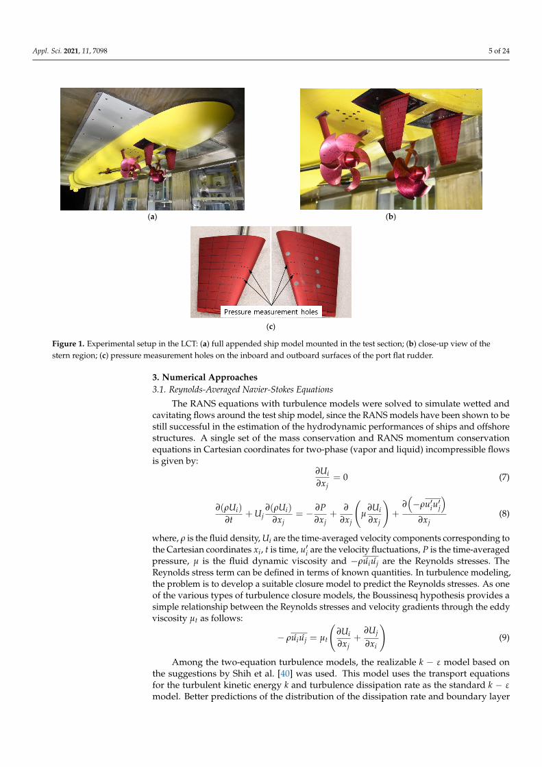
Figure 3 shows the surface and field grids around the full appended hull. An un-structured grid based on hexahedral and polyhedral meshes topology was used in the present simulations. To see the grid convergence on rudder forces, three grids called coarse, medium, and fine with 5.2 M, 7.5 M, and 11 M cells, respectively, were generated by a refinement ratio of √2. A prism layer was used to generate orthogonal prismatic cells next to the wall surfaces, in which the height of the first cells from the wall was determined so that the dimensionless wall distance was set to be 70 or less. Here, all grids had 11 prism grid layers to have a proper resolution of the boundary layer around the hull, pro-peller, and rudder. Especially, an overset grid was adopted to consider the rotations of each rudder in the starboard and port side at a given rudder angle. The present computa-tions were carried out on a Linux-based PC cluster system whose each node has 20 In-tel®_Xeon® 2.40 GHz processors. All runs used a total of 280 processors.

Figure 2. Computational domain: (a) computational domain of the ship model and boundaryconditions; (b) starboard and port rotational regions containing the propellers.

Figure 3 shows the surface and field grids around the full appended hull. An un-structured grid based on hexahedral and polyhedral meshes topology was used in thepresent simulations. To see the grid convergence on rudder forces, three grids called coarse,medium, and fine with 5.2 M, 7.5 M, and 11 M cells, respectively, were generated by arefinement ratio of

√2. A prism layer was used to generate orthogonal prismatic cells next

to the wall surfaces, in which the height of the first cells from the wall was determined sothat the dimensionless wall distance y+ was set to be 70 or less. Here, all grids had 11 prismgrid layers to have a proper resolution of the boundary layer around the hull, propeller, andrudder. Especially, an overset grid was adopted to consider the rotations of each rudder inthe starboard and port side at a given rudder angle. The present computations were carriedout on a Linux-based PC cluster system whose each node has 20 Intel®_Xeon® 2.40 GHzprocessors. All runs used a total of 280 processors.

Appl. Sci. 2021, 11, 7098 8 of 24Appl. Sci. 2021, 11, x FOR PEER REVIEW 8 of 24

(a) (b)

(c)

Figure 3. Computational surface and field grid distributions around the hull, propeller, and rudder: (a) grid distribution on the full appended hull surface; (b) field grids on the longitudinal plane pass-ing through the center of the port rudder; (c) field grids on the transverse plane passing through the center of the propeller.

4. Results and Discussions 4.1. Validation of the Flow around a Flat Rudder 4.1.1. Pressure Distributions

The measured and calculated pressure distributions for wetted flow along the two-chord lines of the port side (PRT) flat rudder are shown in Figure 4 at the rudder angle of δR = 0° and a ship speed of 18 knots. Due to the angle of attack of the flow into the rudder induced by the propeller, it was observed that the inboard of the rudder became the pres-sure side, and the outboard corresponded to the suction side. It is seen that the pressures on the inboard and outboard surfaces differ more significantly at the span location of z/s = 0.6 as seen in Figure 4b, which means the inflow angle varies at each spanwise location at a given rudder angle condition. For a surface combatant having rudder geometry and propeller-rudder configuration similar to the test model proposed by Shen et al. [32], the inflow angle distribution showed a maximum value at the span location of about z/s = 0.66. The minimum pressure of the outboard surface is rather large even at δR = 0° and increased significantly with an increase in the rudder angle. This result indicates that cav-itation inception and cavitation erosion are expected to occur at higher rudder angles. The influences of the inflow angles can be effectively compensated by applying different twist angles in the spanwise direction of a rudder. The current numerical calculations were ob-tained by solving the hull-propeller-rudder interaction of the target ship model under the same conditions of the LCT model tests, showing a good agreement with the measured pressure distributions. This indicates that the numerical approach used in the present study is able to adequately estimate rudder performances. Although the overall difference between the grids used in this result is not large as seen in the figure, the fine grid shows a more reasonable agreement.

Figure 3. Computational surface and field grid distributions around the hull, propeller, and rudder: (a) grid distributionon the full appended hull surface; (b) field grids on the longitudinal plane passing through the center of the port rudder;(c) field grids on the transverse plane passing through the center of the propeller.

4. Results and Discussions4.1. Validation of the Flow around a Flat Rudder4.1.1. Pressure Distributions

The measured and calculated pressure distributions for wetted flow along the two-chord lines of the port side (PRT) flat rudder are shown in Figure 4 at the rudder angleof δR = 0◦ and a ship speed of 18 knots. Due to the angle of attack of the flow into therudder induced by the propeller, it was observed that the inboard of the rudder becamethe pressure side, and the outboard corresponded to the suction side. It is seen thatthe pressures on the inboard and outboard surfaces differ more significantly at the spanlocation of z/s = 0.6 as seen in Figure 4b, which means the inflow angle varies at eachspanwise location at a given rudder angle condition. For a surface combatant havingrudder geometry and propeller-rudder configuration similar to the test model proposedby Shen et al. [32], the inflow angle distribution showed a maximum value at the spanlocation of about z/s = 0.66. The minimum pressure of the outboard surface is rather largeeven at δR = 0◦ and increased significantly with an increase in the rudder angle. This resultindicates that cavitation inception and cavitation erosion are expected to occur at higherrudder angles. The influences of the inflow angles can be effectively compensated byapplying different twist angles in the spanwise direction of a rudder. The current numericalcalculations were obtained by solving the hull-propeller-rudder interaction of the targetship model under the same conditions of the LCT model tests, showing a good agreementwith the measured pressure distributions. This indicates that the numerical approach usedin the present study is able to adequately estimate rudder performances. Although theoverall difference between the grids used in this result is not large as seen in the figure, thefine grid shows a more reasonable agreement.

Appl. Sci. 2021, 11, 7098 9 of 24Appl. Sci. 2021, 11, x FOR PEER REVIEW 9 of 24

(a)

(b)

Figure 4. Pressure distributions along the chord lines on the flat rudder: (a) z/s = 0.45; (b) z/s = 0.6.

4.1.2. Surface Cavitation Figure 5 shows the predicted surface cavitation on the flat rudder with that observed

in the LCT model tests at the rudder angles of δR = 0°, −4°, −8° and −12° and a ship speed of 30 knots. Under all conditions, surface cavitation on the outer surface of the port rudder and the inner surface of the starboard side (STB) rudder is seen. The main difference be-tween the numerical and experimental results was that in the experiment, complicated cloud-cavitation was formed downstream just after the sheet cavitation inception at the leading edge of the rudder. Since the present numerical study used the RANS equations as the governing equations of cavitating flows and the VOF method which is a grid-based Eulerian method for cavitation modeling, it was difficult to precisely capture the behavior of cloud cavitation of particle-like characteristics which vary over a short time. However, it can be noted that the current numerical results agree qualitatively with the experimental results regarding the range and amount of cavitation occurrence according to the change in rudder angle. As expected from the previous results of the pressure distributions along the chord lines, the surface cavitation inception is seen around the region of z/s = 0.7 even at δR = 0°. From this cavitation inception, the rudder cavitation significantly expanded in the chord and span directions as the rudder angle increased. In addition, the tip cavitation inception was detected at the leading edge at δR = 0°. The current study also tried to min-imize this kind of cavitation by modifying the tip geometry. This result will be shortly discussed later.

Figure 4. Pressure distributions along the chord lines on the flat rudder: (a) z/s = 0.45; (b) z/s = 0.6.

4.1.2. Surface Cavitation

Figure 5 shows the predicted surface cavitation on the flat rudder with that observedin the LCT model tests at the rudder angles of δR = 0◦, −4◦, −8◦ and −12◦ and a shipspeed of 30 knots. Under all conditions, surface cavitation on the outer surface of the portrudder and the inner surface of the starboard side (STB) rudder is seen. The main differencebetween the numerical and experimental results was that in the experiment, complicatedcloud-cavitation was formed downstream just after the sheet cavitation inception at theleading edge of the rudder. Since the present numerical study used the RANS equations asthe governing equations of cavitating flows and the VOF method which is a grid-basedEulerian method for cavitation modeling, it was difficult to precisely capture the behaviorof cloud cavitation of particle-like characteristics which vary over a short time. However, itcan be noted that the current numerical results agree qualitatively with the experimentalresults regarding the range and amount of cavitation occurrence according to the change inrudder angle. As expected from the previous results of the pressure distributions along

Appl. Sci. 2021, 11, 7098 10 of 24

the chord lines, the surface cavitation inception is seen around the region of z/s = 0.7 evenat δR = 0◦. From this cavitation inception, the rudder cavitation significantly expanded inthe chord and span directions as the rudder angle increased. In addition, the tip cavitationinception was detected at the leading edge at δR = 0◦. The current study also tried tominimize this kind of cavitation by modifying the tip geometry. This result will be shortlydiscussed later.


(a) (b)

(c) (d)

Figure 5. Experimental observation and numerical prediction of surface cavitation on the twin flat rudders: (a) δR = 0°; (b) δR = −4°; (c) δR = −8°; (d) δR = −12°.

4.1.3. Forces and Moment The measured and predicted lift and drag forces and moment for the flat rudder at

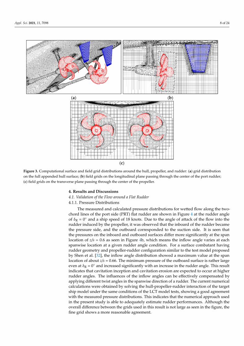
30 knots and cavitating flow condition are shown in Figure 6. The moment was measured with respect to the rudder stock axis that is the center of rotation of the rudder. In Figure 6a, the lift coefficients are seen to linearly change when both starboard and port rudders have no or slight cavitation occurrence. At rudder angles larger than δR = 8° in absolute value for each side of the twin rudder with significant cavitation, it is seen that the lift forces vary nonlinearly and decrease somewhat because of massive cavitation occurrence. The zero-lift angles are placed at around −4.69° and 4.91°, respectively, which was due to the inflow angles induced by the propeller. The zero-lift angle can be expected to become around 0° for a twisted rudder applied with appropriate inflow angles. The trend of this measured lift force is closely followed by the current numerical results. The difference between the experimental and numerical results was caused by the limitation of the cur-rent numerical approach where cloud type cavitation occurs as discussed earlier. For each rudder with surface cavitation, the predicted lift forces are smaller than the experimental values because the predicted cavitation was nearly attached to the rudder surface unlike the cloud type cavitation which detached off the rudder surface, as observed in the exper-iment, and increased the suction side pressures. In Figure 6b,c, similar trends are also seen in the comparisons of the drag force and moment. Where the cavitation effect is not sig-nificant, the predicted forces and moment show a very good agreement with the experi-mental data. When the grid dependence in the results for the rudder angles of δR = 0°, 8°, and 16° was examined, the difference between the grids was not significant. From these results, it can be noted that the current numerical approach shows a reasonable accuracy enough to qualitatively estimate the hydrodynamic forces of rudders.

(a) (b) (c)

Figure 5. Experimental observation and numerical prediction of surface cavitation on the twin flat rudders: (a) δR = 0◦;(b) δR = −4◦; (c) δR = −8◦; (d) δR = −12◦.

4.1.3. Forces and Moment

The measured and predicted lift and drag forces and moment for the flat rudder at30 knots and cavitating flow condition are shown in Figure 6. The moment was measuredwith respect to the rudder stock axis that is the center of rotation of the rudder. In Figure 6a,the lift coefficients are seen to linearly change when both starboard and port rudders haveno or slight cavitation occurrence. At rudder angles larger than δR = 8◦ in absolute valuefor each side of the twin rudder with significant cavitation, it is seen that the lift forces varynonlinearly and decrease somewhat because of massive cavitation occurrence. The zero-liftangles are placed at around −4.69◦ and 4.91◦, respectively, which was due to the inflowangles induced by the propeller. The zero-lift angle can be expected to become around 0◦

for a twisted rudder applied with appropriate inflow angles. The trend of this measuredlift force is closely followed by the current numerical results. The difference between theexperimental and numerical results was caused by the limitation of the current numericalapproach where cloud type cavitation occurs as discussed earlier. For each rudder withsurface cavitation, the predicted lift forces are smaller than the experimental values becausethe predicted cavitation was nearly attached to the rudder surface unlike the cloud typecavitation which detached off the rudder surface, as observed in the experiment, andincreased the suction side pressures. In Figure 6b,c, similar trends are also seen in thecomparisons of the drag force and moment. Where the cavitation effect is not significant,the predicted forces and moment show a very good agreement with the experimental data.When the grid dependence in the results for the rudder angles of δR = 0◦, 8◦, and 16◦

was examined, the difference between the grids was not significant. From these results, itcan be noted that the current numerical approach shows a reasonable accuracy enough toqualitatively estimate the hydrodynamic forces of rudders.

Appl. Sci. 2021, 11, 7098 11 of 24


(a) (b)

(c) (d)

Figure 5. Experimental observation and numerical prediction of surface cavitation on the twin flat rudders: (a) δR = 0°; (b) δR = −4°; (c) δR = −8°; (d) δR = −12°.

4.1.3. Forces and Moment The measured and predicted lift and drag forces and moment for the flat rudder at

30 knots and cavitating flow condition are shown in Figure 6. The moment was measured with respect to the rudder stock axis that is the center of rotation of the rudder. In Figure 6a, the lift coefficients are seen to linearly change when both starboard and port rudders have no or slight cavitation occurrence. At rudder angles larger than δR = 8° in absolute value for each side of the twin rudder with significant cavitation, it is seen that the lift forces vary nonlinearly and decrease somewhat because of massive cavitation occurrence. The zero-lift angles are placed at around −4.69° and 4.91°, respectively, which was due to the inflow angles induced by the propeller. The zero-lift angle can be expected to become around 0° for a twisted rudder applied with appropriate inflow angles. The trend of this measured lift force is closely followed by the current numerical results. The difference between the experimental and numerical results was caused by the limitation of the cur-rent numerical approach where cloud type cavitation occurs as discussed earlier. For each rudder with surface cavitation, the predicted lift forces are smaller than the experimental values because the predicted cavitation was nearly attached to the rudder surface unlike the cloud type cavitation which detached off the rudder surface, as observed in the exper-iment, and increased the suction side pressures. In Figure 6b,c, similar trends are also seen in the comparisons of the drag force and moment. Where the cavitation effect is not sig-nificant, the predicted forces and moment show a very good agreement with the experi-mental data. When the grid dependence in the results for the rudder angles of δR = 0°, 8°, and 16° was examined, the difference between the grids was not significant. From these results, it can be noted that the current numerical approach shows a reasonable accuracy enough to qualitatively estimate the hydrodynamic forces of rudders.

(a) (b) (c)

Figure 6. Measured and numerically predicted rudder forces and moment for the twin flat rudders: (a) lift force; (b) dragforce; (c) moment.

4.2. Prediction and Correction of Twist Angles

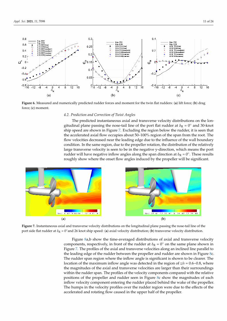
The predicted instantaneous axial and transverse velocity distributions on the lon-gitudinal plane passing the nose-tail line of the port flat rudder at δR = 0◦ and 30-knotship speed are shown in Figure 7. Excluding the region below the rudder, it is seen thatthe accelerated axial flow occupies about 50–100% region of the span from the root. Theflow velocities decreased near the leading edge due to the influence of the wall boundarycondition. In the same region, due to the propeller rotation, the distribution of the relativelylarge transverse velocity is seen to be in the negative y-direction, which means the portrudder will have negative inflow angles along the span direction at δR = 0◦. These resultsroughly show where the onset flow angles induced by the propeller will be significant.


Figure 6. Measured and numerically predicted rudder forces and moment for the twin flat rudders: (a) lift force; (b) drag force; (c) moment.

4.2. Prediction and Correction of Twist Angles The predicted instantaneous axial and transverse velocity distributions on the longi-

tudinal plane passing the nose-tail line of the port flat rudder at δR = 0° and 30-knot ship speed are shown in Figure 7. Excluding the region below the rudder, it is seen that the accelerated axial flow occupies about 50–100% region of the span from the root. The flow velocities decreased near the leading edge due to the influence of the wall boundary con-dition. In the same region, due to the propeller rotation, the distribution of the relatively large transverse velocity is seen to be in the negative y-direction, which means the port rudder will have negative inflow angles along the span direction at δR = 0°. These results roughly show where the onset flow angles induced by the propeller will be significant.

Figures 8a,b show the time-averaged distributions of axial and transverse velocity components, respectively, in front of the rudder at δR = 0° on the same plane shown in Figure 7. The profiles of the axial and transverse velocities along an inclined line parallel to the leading edge of the rudder between the propeller and rudder are shown in Figure 8c. The rudder span region where the inflow angle is significant is shown to be clearer. The location of the maximum inflow angle was detected in the region of z/s = 0.6~0.8, where the magnitudes of the axial and transverse velocities are larger than their surround-ings within the rudder span. The profiles of the velocity components compared with the relative positions of the propeller and rudder seen in Figure 8c show the magnitudes of each inflow velocity component entering the rudder placed behind the wake of the pro-peller. The humps in the velocity profiles over the rudder region were due to the effects of the accelerated and rotating flow caused in the upper half of the propeller.

Figure 9 shows a transverse plane between the propeller and the rudder aligned with the inclined leading edge of the flat rudder keeping a distance of 0.26 in which velocity distributions of the axial and transverse components were measured to obtain the inflow angles.

(a) (b)

Figure 7. Instantaneous axial and transverse velocity distributions on the longitudinal plane passing the nose-tail line of the port side flat rudder at δR = 0°and 26 knot ship speed: (a) axial velocity distribution; (b) transverse velocity distribution.

(a) (b)

Figure 7. Instantaneous axial and transverse velocity distributions on the longitudinal plane passing the nose-tail line of theport side flat rudder at δR = 0◦and 26 knot ship speed: (a) axial velocity distribution; (b) transverse velocity distribution.

Figure 8a,b show the time-averaged distributions of axial and transverse velocitycomponents, respectively, in front of the rudder at δR = 0◦ on the same plane shown inFigure 7. The profiles of the axial and transverse velocities along an inclined line parallel tothe leading edge of the rudder between the propeller and rudder are shown in Figure 8c.The rudder span region where the inflow angle is significant is shown to be clearer. Thelocation of the maximum inflow angle was detected in the region of z/s = 0.6~0.8, wherethe magnitudes of the axial and transverse velocities are larger than their surroundingswithin the rudder span. The profiles of the velocity components compared with the relativepositions of the propeller and rudder seen in Figure 8c show the magnitudes of eachinflow velocity component entering the rudder placed behind the wake of the propeller.The humps in the velocity profiles over the rudder region were due to the effects of theaccelerated and rotating flow caused in the upper half of the propeller.

Appl. Sci. 2021, 11, 7098 12 of 24


Figure 6. Measured and numerically predicted rudder forces and moment for the twin flat rudders: (a) lift force; (b) drag force; (c) moment.

4.2. Prediction and Correction of Twist Angles The predicted instantaneous axial and transverse velocity distributions on the longi-

tudinal plane passing the nose-tail line of the port flat rudder at δR = 0° and 30-knot ship speed are shown in Figure 7. Excluding the region below the rudder, it is seen that the accelerated axial flow occupies about 50–100% region of the span from the root. The flow velocities decreased near the leading edge due to the influence of the wall boundary con-dition. In the same region, due to the propeller rotation, the distribution of the relatively large transverse velocity is seen to be in the negative y-direction, which means the port rudder will have negative inflow angles along the span direction at δR = 0°. These results roughly show where the onset flow angles induced by the propeller will be significant.

Figures 8a,b show the time-averaged distributions of axial and transverse velocity components, respectively, in front of the rudder at δR = 0° on the same plane shown in Figure 7. The profiles of the axial and transverse velocities along an inclined line parallel to the leading edge of the rudder between the propeller and rudder are shown in Figure 8c. The rudder span region where the inflow angle is significant is shown to be clearer. The location of the maximum inflow angle was detected in the region of z/s = 0.6~0.8, where the magnitudes of the axial and transverse velocities are larger than their surround-ings within the rudder span. The profiles of the velocity components compared with the relative positions of the propeller and rudder seen in Figure 8c show the magnitudes of each inflow velocity component entering the rudder placed behind the wake of the pro-peller. The humps in the velocity profiles over the rudder region were due to the effects of the accelerated and rotating flow caused in the upper half of the propeller.

Figure 9 shows a transverse plane between the propeller and the rudder aligned with the inclined leading edge of the flat rudder keeping a distance of 0.26 in which velocity distributions of the axial and transverse components were measured to obtain the inflow angles.

(a) (b)

Figure 7. Instantaneous axial and transverse velocity distributions on the longitudinal plane passing the nose-tail line of the port side flat rudder at δR = 0°and 26 knot ship speed: (a) axial velocity distribution; (b) transverse velocity distribution.

(a) (b)


(c)

Figure 8. Time-averaged distributions of axial and transverse velocity components and the profiles of those two velocities in front of the leading edge of the flat rudder: (a) axial velocity distribution; (b) transverse velocity distribution; (c) axial and transverse velocity profiles.

Figure 9. Measurement plane location in which inflow angles were predicted using the axial and transverse velocities.

Figure 10 shows the numerically predicted flow angle distribution on the measure-ment plane shown in Figure 9. Due to the propeller rotation, the onset flow angle has opposite signs at the upper and lower propeller planes as seen in Figure 10a. The maxi-mum inflow angles with opposite signs were observed around the radius of 0.56 in the 7 o’clock and 1 o’clock positions, respectively. The predicted inflow angles along the rud-der span direction for the rudder angle range of δR = −16°–16° are shown in Figure 10b. The distribution of the inflow angles along the rudder span direction is in the range of 0°–11° for the rudder angle of δR = 0°. The range of the maximum inflow angle experienced by the rudder at the rudder angle range of δR = −16°–16° corresponds to about 5°–15°.

Figure 8. Time-averaged distributions of axial and transverse velocity components and the profilesof those two velocities in front of the leading edge of the flat rudder: (a) axial velocity distribution;(b) transverse velocity distribution; (c) axial and transverse velocity profiles.

Figure 9 shows a transverse plane between the propeller and the rudder alignedwith the inclined leading edge of the flat rudder keeping a distance of 0.26DP in whichvelocity distributions of the axial and transverse components were measured to obtain theinflow angles.


(c)

Figure 8. Time-averaged distributions of axial and transverse velocity components and the profiles of those two velocities in front of the leading edge of the flat rudder: (a) axial velocity distribution; (b) transverse velocity distribution; (c) axial and transverse velocity profiles.

Figure 9. Measurement plane location in which inflow angles were predicted using the axial and transverse velocities.

Figure 10 shows the numerically predicted flow angle distribution on the measure-ment plane shown in Figure 9. Due to the propeller rotation, the onset flow angle has opposite signs at the upper and lower propeller planes as seen in Figure 10a. The maxi-mum inflow angles with opposite signs were observed around the radius of 0.56 in the 7 o’clock and 1 o’clock positions, respectively. The predicted inflow angles along the rud-der span direction for the rudder angle range of δR = −16°–16° are shown in Figure 10b. The distribution of the inflow angles along the rudder span direction is in the range of 0°–11° for the rudder angle of δR = 0°. The range of the maximum inflow angle experienced by the rudder at the rudder angle range of δR = −16°–16° corresponds to about 5°–15°.

Figure 9. Measurement plane location in which inflow angles were predicted using the axial andtransverse velocities.

Figure 10 shows the numerically predicted flow angle distribution on the measurementplane shown in Figure 9. Due to the propeller rotation, the onset flow angle has opposite

Appl. Sci. 2021, 11, 7098 13 of 24

signs at the upper and lower propeller planes as seen in Figure 10a. The maximum inflowangles with opposite signs were observed around the radius of 0.56RP in the 7 o’clockand 1 o’clock positions, respectively. The predicted inflow angles along the rudder spandirection for the rudder angle range of δR = −16◦–16◦ are shown in Figure 10b. Thedistribution of the inflow angles along the rudder span direction is in the range of 0◦–11◦

for the rudder angle of δR = 0◦. The range of the maximum inflow angle experienced bythe rudder at the rudder angle range of δR = −16◦–16◦ corresponds to about 5◦–15◦.


(a) (b)

Figure 10. Numerically predicted inflow angle distribution on a transverse plane in front of the port flat rudder and com-parison of inflow angles predicted and measured according to rudder angle: (a) inflow angle distribution on the measure-ment plane shown in Figure 9; (b) inflow angles in the span direction according to rudder angle.

The initial twisted rudder model was designed based on the predicted inflow angle distribution along the rudder span at δR = 0°. However, it was found that the twist angles can be overpredicted when extracted from the leading edge lines projected onto the meas-urement plane shown in Figure 9. When the streamline distribution on the cross-sections in the span direction of the port rudder, as shown in Figure 11, was examined, it was found that the inflow angles computed at the initial prediction points should be corrected. At the selected span locations of z/s = 0.3, 0.5, 0.7, and 0.9, the streamlines passing through the initial measurement points are seen to be slightly biased toward the outboard direction of the port rudder which leads to a slight overestimation of the predicted initial inflow angles. The correction of the flow angle distribution was done by searching the streamline that had the stagnation point on the leading edge of the rudder. In this work, the maxi-mum inflow angle was estimated to be about 3° smaller.

Figure 12 compares the twist angles before and after correction along the rudder span direction. The symbols show the inflow angles calculated at each span position, and the lines are the results of the interpolation of those angles using polynomial curves. The in-termediate twist angle distribution was extracted to validate the final corrected twist an-gles by applying them together to the numerical and experimental analyses. The corrected twist angle distribution had a range from 0° to about 8.1°, while the intermediate twist angles were in a range from 0° to about 9.2°.

(a) (b)

Figure 10. Numerically predicted inflow angle distribution on a transverse plane in front of the port flat rudder andcomparison of inflow angles predicted and measured according to rudder angle: (a) inflow angle distribution on themeasurement plane shown in Figure 9; (b) inflow angles in the span direction according to rudder angle.

The initial twisted rudder model was designed based on the predicted inflow angledistribution along the rudder span at δR = 0◦. However, it was found that the twistangles can be overpredicted when extracted from the leading edge lines projected ontothe measurement plane shown in Figure 9. When the streamline distribution on the cross-sections in the span direction of the port rudder, as shown in Figure 11, was examined,it was found that the inflow angles computed at the initial prediction points should becorrected. At the selected span locations of z/s = 0.3, 0.5, 0.7, and 0.9, the streamlines passingthrough the initial measurement points are seen to be slightly biased toward the outboarddirection of the port rudder which leads to a slight overestimation of the predicted initialinflow angles. The correction of the flow angle distribution was done by searching thestreamline that had the stagnation point on the leading edge of the rudder. In this work,the maximum inflow angle was estimated to be about 3◦ smaller.

Figure 12 compares the twist angles before and after correction along the rudderspan direction. The symbols show the inflow angles calculated at each span position,and the lines are the results of the interpolation of those angles using polynomial curves.The intermediate twist angle distribution was extracted to validate the final correctedtwist angles by applying them together to the numerical and experimental analyses. Thecorrected twist angle distribution had a range from 0◦ to about 8.1◦, while the intermediatetwist angles were in a range from 0◦ to about 9.2◦.

Appl. Sci. 2021, 11, 7098 14 of 24


(a) (b)

Figure 10. Numerically predicted inflow angle distribution on a transverse plane in front of the port flat rudder and com-parison of inflow angles predicted and measured according to rudder angle: (a) inflow angle distribution on the measure-ment plane shown in Figure 9; (b) inflow angles in the span direction according to rudder angle.

The initial twisted rudder model was designed based on the predicted inflow angle distribution along the rudder span at δR = 0°. However, it was found that the twist angles can be overpredicted when extracted from the leading edge lines projected onto the meas-urement plane shown in Figure 9. When the streamline distribution on the cross-sections in the span direction of the port rudder, as shown in Figure 11, was examined, it was found that the inflow angles computed at the initial prediction points should be corrected. At the selected span locations of z/s = 0.3, 0.5, 0.7, and 0.9, the streamlines passing through the initial measurement points are seen to be slightly biased toward the outboard direction of the port rudder which leads to a slight overestimation of the predicted initial inflow angles. The correction of the flow angle distribution was done by searching the streamline that had the stagnation point on the leading edge of the rudder. In this work, the maxi-mum inflow angle was estimated to be about 3° smaller.

Figure 12 compares the twist angles before and after correction along the rudder span direction. The symbols show the inflow angles calculated at each span position, and the lines are the results of the interpolation of those angles using polynomial curves. The in-termediate twist angle distribution was extracted to validate the final corrected twist an-gles by applying them together to the numerical and experimental analyses. The corrected twist angle distribution had a range from 0° to about 8.1°, while the intermediate twist angles were in a range from 0° to about 9.2°.

(a) (b)


(c) (d)

Figure 11. Prediction and correction points at which inflow angles were calculated by using the axial and transverse ve-locities: (a) z/s = 0.3; (b) z/s = 0.5; (c) z/s = 0.7; (d) z/s = 0.9.

Figure 12. Distributions of twist angles along the span direction.

4.3. Hydrodynamic Performances of Twisted Rudders Three twisted rudders shown in Figure 13 were made respectively by rotating each

cross-section of the flat rudder around the mid-chord point according to the initial, inter-mediate, and final corrected twist angles described in Figure 12. Afterward, the three twisted rudders were named TR-ini, TR-int, and TR-fin. To examine the cavitation perfor-mance of the tip area, the TR-ini and TR-int twist rudders were attached with an end plate and a rounded tip was tested for the TR-fin model. For the investigation of the hydrody-namic performance of the twisted rudders, the numerical simulations of cavitating flows were carried out at 30-knot ship speed and the same propeller rotation condition used for the flat rudder as shown in Table 2.

(a) (b) (c)

Figure 13. Designed twisted rudders: (a) TR-ini; (b) TR-int; (c) TR-fin.

The effectiveness of the twisted rudder TR-fin on the compensation of the onset flow angles was confirmed by recalculating the inflow angles from the distribution of the streamlines over each cross-section in the rudder span direction at δR = 0° as shown in

Figure 11. Prediction and correction points at which inflow angles were calculated by using the axial and transversevelocities: (a) z/s = 0.3; (b) z/s = 0.5; (c) z/s = 0.7; (d) z/s = 0.9.


(c) (d)





(a) (b) (c)




4.3. Hydrodynamic Performances of Twisted Rudders

Three twisted rudders shown in Figure 13 were made respectively by rotating eachcross-section of the flat rudder around the mid-chord point according to the initial, interme-diate, and final corrected twist angles described in Figure 12. Afterward, the three twistedrudders were named TR-ini, TR-int, and TR-fin. To examine the cavitation performanceof the tip area, the TR-ini and TR-int twist rudders were attached with an end plate and arounded tip was tested for the TR-fin model. For the investigation of the hydrodynamicperformance of the twisted rudders, the numerical simulations of cavitating flows werecarried out at 30-knot ship speed and the same propeller rotation condition used for theflat rudder as shown in Table 2.

The effectiveness of the twisted rudder TR-fin on the compensation of the onsetflow angles was confirmed by recalculating the inflow angles from the distribution ofthe streamlines over each cross-section in the rudder span direction at δR = 0◦ as shownin Figure 14. While the inflow angles are seen to be slightly overcompensated by theTR-ini rudder, nearly zero angles of attack and symmetrical pressure distributions are

Appl. Sci. 2021, 11, 7098 15 of 24

shown for the TR-fin rudder. The intermediate version, TR-int rudder presented the nextbest improvement.


(c) (d)





(a) (b) (c)





Figure 14. While the inflow angles are seen to be slightly overcompensated by the TR-ini rudder, nearly zero angles of attack and symmetrical pressure distributions are shown for the TR-fin rudder. The intermediate version, TR-int rudder presented the next best im-provement.

(a) (b)

(c) (d)

(e) (f)

Figure 14. Streamline and pressure distributions on the cross sections in the span direction of three twisted rudders: (a) TR-ini at z/s = 0.5; (b) TR-int at z/s = 0.5; (c) TR-fin at z/s = 0.5; (d) TR-ini at z/s = 0.7; (e) TR-int at z/s = 0.7; (f) TR-fin at z/s = 0.7.

Figure 15 shows the pressure distributions along the rudder span direction from z/s = 0.4–0.9 for the twisted rudders compared with those of the flat rudder. As seen in Figure 14, the pressure distributions for the TR-fin rudder are very close to each other on the inboard and outboard surfaces except for z/s = 0.9, where the three-dimensional flow effect near the tip region can be significant. The predicted pressure distributions for the flat rud-der vary largely on each surface, especially at z/s = 0.7~0.9, at which the cavitation incep-tion appeared on the outboard surface. These results indicate that the surface cavitation inception phenomenon on the twisted rudder will be significantly improved compared with the flat rudder.

Figure 14. Streamline and pressure distributions on the cross sections in the span direction of three twisted rudders:(a) TR-ini at z/s = 0.5; (b) TR-int at z/s = 0.5; (c) TR-fin at z/s = 0.5; (d) TR-ini at z/s = 0.7; (e) TR-int at z/s = 0.7; (f) TR-fin atz/s = 0.7.

Figure 15 shows the pressure distributions along the rudder span direction fromz/s = 0.4–0.9 for the twisted rudders compared with those of the flat rudder. As seen inFigure 14, the pressure distributions for the TR-fin rudder are very close to each otheron the inboard and outboard surfaces except for z/s = 0.9, where the three-dimensional

Appl. Sci. 2021, 11, 7098 16 of 24

flow effect near the tip region can be significant. The predicted pressure distributionsfor the flat rudder vary largely on each surface, especially at z/s = 0.7~0.9, at whichthe cavitation inception appeared on the outboard surface. These results indicate thatthe surface cavitation inception phenomenon on the twisted rudder will be significantlyimproved compared with the flat rudder.


(a) (b)

(c) (d)

Figure 15. Pressure distributions along the chord lines on the twisted rudders: (a) z/s = 0.4; (b) z/s = 0.6; (c) z/s = 0.7; (d) z/s = 0.9.

Figures 16–18 show the predicted and observed surface cavitation on the flat and three twisted rudders at the rudder angles of δR = −6°, −8°, and −16°, respectively. As shown in Figure 5, the surface cavitation inception was detected even at δR = 0° for the flat rudder. For the twisted rudders, no surface cavitation was observed before δR = −6° in both the experiments and numerical simulations. While surface cavitation appeared on the out-board surface of the port flat rudder at δR = −6°, the same appeared on the inboard surfaces of each starboard twisted rudder. This was because each inflow angle distribution in-duced by the propellers on the starboard and port side was in opposite sign and both side rudders of a twin twisted rudder were made based on these twist angles. The starboard twisted rudder was unable to effectively compensate the inflow angles at negative rudder angles, and in the same way, the port twisted rudder was disadvantageous at positive rudder angles. As expected from the pressure distributions shown in Figure 15, it is seen that the cavitation occurrence is significantly decreased in the TR-fin rudder, followed by the TR-int and TR-ini rudders. Regarding tip cavitation inception, the rudder tip cavita-tion inception was also detected at the mid-chord of the tip on each inboard surface of both the starboard and port TR-ini and TR-int rudders equipped with a tip end plate at δR = 0°. On the other hand, such cavitation was observed on the TR-fin rudder above δR = −6°. This indicates that the rounded tip applied to the TR-fin rudder is more useful than the end plate in reducing the tip cavitation.

Figure 15. Pressure distributions along the chord lines on the twisted rudders: (a) z/s = 0.4; (b) z/s = 0.6;(c) z/s = 0.7; (d) z/s = 0.9.

Figures 16–18 show the predicted and observed surface cavitation on the flat andthree twisted rudders at the rudder angles of δR = −6◦, −8◦, and −16◦, respectively. Asshown in Figure 5, the surface cavitation inception was detected even at δR = 0◦ for the flatrudder. For the twisted rudders, no surface cavitation was observed before δR = −6◦ inboth the experiments and numerical simulations. While surface cavitation appeared onthe outboard surface of the port flat rudder at δR = −6◦, the same appeared on the inboardsurfaces of each starboard twisted rudder. This was because each inflow angle distributioninduced by the propellers on the starboard and port side was in opposite sign and both siderudders of a twin twisted rudder were made based on these twist angles. The starboardtwisted rudder was unable to effectively compensate the inflow angles at negative rudderangles, and in the same way, the port twisted rudder was disadvantageous at positiverudder angles. As expected from the pressure distributions shown in Figure 15, it is seenthat the cavitation occurrence is significantly decreased in the TR-fin rudder, followed bythe TR-int and TR-ini rudders. Regarding tip cavitation inception, the rudder tip cavitationinception was also detected at the mid-chord of the tip on each inboard surface of both thestarboard and port TR-ini and TR-int rudders equipped with a tip end plate at δR = 0◦. Onthe other hand, such cavitation was observed on the TR-fin rudder above δR = −6◦. This

Appl. Sci. 2021, 11, 7098 17 of 24

indicates that the rounded tip applied to the TR-fin rudder is more useful than the endplate in reducing the tip cavitation.


(a) (b)

(c) (d)

Figure 16. Experimental observation and numerical prediction of surface cavitation on the twin twisted rudders at δR = −6°: (a) flat rudder; (b) TR-ini; (c) TR-int; (d) TR-fin.

(a) (b)

(c) (d)


(a) (b)

(c) (d)


It is seen in Figure 17 that the outboard surface cavitation begins to occur on each port twisted rudder at δR = −8°. The inboard surface cavitation observed on the starboard twisted rudders at δR = −6° is slightly larger at δR = −8°, but it is still the smallest on the TR-fin rudder.

Figure 16. Experimental observation and numerical prediction of surface cavitation on the twin twisted rudders at δR =−6◦:(a) flat rudder; (b) TR-ini; (c) TR-int; (d) TR-fin.


(a) (b)

(c) (d)


(a) (b)

(c) (d)


(a) (b)

(c) (d)





(a) (b)

(c) (d)


(a) (b)

(c) (d)


(a) (b)

(c) (d)




Appl. Sci. 2021, 11, 7098 18 of 24

It is seen in Figure 17 that the outboard surface cavitation begins to occur on eachport twisted rudder at δR = −8◦. The inboard surface cavitation observed on the starboardtwisted rudders at δR = −6◦ is slightly larger at δR = −8◦, but it is still the smallest on theTR-fin rudder.

At the rudder angle of δR = −16◦, severe surface cavitation is seen on all the ruddermodels as shown in Figure 18. For the flat rudder, it is seen that most of the outboardsurface of the port rudder is covered with cavitation. Additionally, the inboard surfacecavitation on the flat rudder started at δR = −14◦. To compare roughly the amount of thecavitation occurrence between the port rudders, the border line of the surface cavitation ofthe port flat rudder was overlaid on the outboard surfaces of the port twisted rudders as adashed line. For the same purpose, the border line of the inboard surface cavitation of thestarboard TR-ini rudder was superposed on the starboard TR-int and TR-fin rudders. Theoutboard surface cavitation on the port twisted rudders is seen to be largely decreased dueto the compensation of the effects of the inflow angles. On the other hand, since a starboardtwisted rudder at a negative rudder angle is disadvantageous in compensating the inflowangles, the inboard surface cavitation of the starboard twisted rudder can be increasedthan that on the flat rudder. For the twisted rudders, it is seen that the starboard surfacecavitation on the TR-fin rudder is smaller than those on the other two twisted rudders.Therefore, these results show that the occurrence of surface cavitation in the TR-fin rudderson the starboard and port side is the smallest, showing the validity of the prediction andcorrection of the inflow angle distribution as described in the previous section.

The measured and predicted lift and drag forces and moment for the three twistedrudders at 30 knots and cavitating flow conditions are shown in Figure 19. As discussedfor the results of the flat rudder in Section 4.1.3, the current numerical results for thetwisted rudders show also a qualitatively good agreement with the experimental data. Theminimum drag coefficients of each twisted rudder on the starboard and port side were foundto be larger than that of the flat rudder at δR = 0◦ shown in Figure 6. In Figure 19a,d,g, theminimum positions are seen to be approximately δR = ±7◦, ±6◦ and ±5◦ for the TR-ini,TR-int, and TR-fin rudders, respectively. When considering the total drag of the starboardand port rudders, the total drag coefficients for the twin TR-ini and TR-int rudders werelarger than that of the twin flat rudder in the current whole rudder angle range. In thenumerical analysis, the total drag coefficient of the twin TR-fin rudders was smaller thanthat of the twin flat rudder above about δR = ±6◦, although this range was different fromthe experimental range of δR= ±4◦~±12◦.

With regard to the effect of the twist angles on rudder lift force, it is seen that eachrudder lift force according to the rudder angle on the starboard and port side is almostsimilar for the TR-fin twisted rudder accounting for a relatively accurate inflow angledistribution as seen in Figure 19b,e,h. In the numerical simulation, the zero-lift angleof both sides of the TR-fin rudder is seen to be almost zero, but in the experiment, it isabout 0.7◦ for the port rudder as seen in Figure 19h. The slope of the total lift force foreach twisted rudder was similar to each other and slightly greater than that of the flatrudder. This means that a twisted rudder will be slightly better than a flat rudder in themaneuvering performance of ships.

Finally, it is seen that each rudder moment on the starboard and port side accordingto the rudder angle as seen in Figure 19c,f,i is getting closer to each other in the order theTR-fin, TR-int, and TR-ini rudders as the lift forces. The maximum moment coefficient wasfound to decrease in the same order. This shows that when an accurate twist angle distri-bution is applied, the rudder moment can be appropriately reduced without a significantreduction in the lift force.

Appl. Sci. 2021, 11, 7098 19 of 24


At the rudder angle of δR = −16°, severe surface cavitation is seen on all the rudder models as shown in Figure 18. For the flat rudder, it is seen that most of the outboard surface of the port rudder is covered with cavitation. Additionally, the inboard surface cavitation on the flat rudder started at δR = −14°. To compare roughly the amount of the cavitation occurrence between the port rudders, the border line of the surface cavitation of the port flat rudder was overlaid on the outboard surfaces of the port twisted rudders as a dashed line. For the same purpose, the border line of the inboard surface cavitation of the starboard TR-ini rudder was superposed on the starboard TR-int and TR-fin rud-ders. The outboard surface cavitation on the port twisted rudders is seen to be largely decreased due to the compensation of the effects of the inflow angles. On the other hand, since a starboard twisted rudder at a negative rudder angle is disadvantageous in com-pensating the inflow angles, the inboard surface cavitation of the starboard twisted rudder can be increased than that on the flat rudder. For the twisted rudders, it is seen that the starboard surface cavitation on the TR-fin rudder is smaller than those on the other two twisted rudders. Therefore, these results show that the occurrence of surface cavitation in the TR-fin rudders on the starboard and port side is the smallest, showing the validity of the prediction and correction of the inflow angle distribution as described in the previous section.

The measured and predicted lift and drag forces and moment for the three twisted rudders at 30 knots and cavitating flow conditions are shown in Figure 19. As discussed for the results of the flat rudder in Section 4.1.3, the current numerical results for the twisted rudders show also a qualitatively good agreement with the experimental data. The minimum drag coefficients of each twisted rudder on the starboard and port side were found to be larger than that of the flat rudder at δR = 0° shown in Figure 6. In Figures 19a,d,g, the minimum positions are seen to be approximately δR = ±7°, ±6° and ±5° for the TR-ini, TR-int, and TR-fin rudders, respectively. When considering the total drag of the starboard and port rudders, the total drag coefficients for the twin TR-ini and TR-int rud-ders were larger than that of the twin flat rudder in the current whole rudder angle range. In the numerical analysis, the total drag coefficient of the twin TR-fin rudders was smaller than that of the twin flat rudder above about δR = ±6°, although this range was different from the experimental range of δR= ±4°~±12°.

(a) (b) (c)


(d) (e) (f)

(g) (h) (i)

Figure 19. Measured and numerically predicted rudder forces and moment for the twisted rudders on the starboard and port side: (a) drag force for TR-ini; (b) lift force for TR-ini; (c) moment for TR-ini; (d) drag force for TR-int; (e) lift force for TR-int; (f) moment for TR-int; (g) drag force for TR-fin; (h) lift force for TR-fin; (i) moment for TR-fin.

With regard to the effect of the twist angles on rudder lift force, it is seen that each rudder lift force according to the rudder angle on the starboard and port side is almost similar for the TR-fin twisted rudder accounting for a relatively accurate inflow angle dis-tribution as seen in Figures 19b,e,h. In the numerical simulation, the zero-lift angle of both sides of the TR-fin rudder is seen to be almost zero, but in the experiment, it is about 0.7° for the port rudder as seen in Figure 19h. The slope of the total lift force for each twisted rudder was similar to each other and slightly greater than that of the flat rudder. This means that a twisted rudder will be slightly better than a flat rudder in the maneuvering performance of ships.

Finally, it is seen that each rudder moment on the starboard and port side according to the rudder angle as seen in Figure 19c,f,i is getting closer to each other in the order the TR-fin, TR-int, and TR-ini rudders as the lift forces. The maximum moment coefficient was found to decrease in the same order. This shows that when an accurate twist angle distribution is applied, the rudder moment can be appropriately reduced without a sig-nificant reduction in the lift force.

4.4. Summary of Twisted Rudder Performances One of the important design criteria in the current work in the development of a

twisted rudder in this study was an improvement in the cavitation performance compared with that of the reference flat rudder at the reference rudder angle of δR = 15°. At the same reference rudder angle, the maintenance of rudder lift performance which affects the ship’s maneuverability, and the reduction of rudder moment applied to the rudder axis were the next important criteria. With respect to the ship’s self-propulsion performance, the final thing was to reduce the drag increase of a twin twisted rudder at δR = 0° up to an appropriate level.

Figure 19. Measured and numerically predicted rudder forces and moment for the twisted rudders on the starboard andport side: (a) drag force for TR-ini; (b) lift force for TR-ini; (c) moment for TR-ini; (d) drag force for TR-int; (e) lift force forTR-int; (f) moment for TR-int; (g) drag force for TR-fin; (h) lift force for TR-fin; (i) moment for TR-fin.

4.4. Summary of Twisted Rudder Performances

One of the important design criteria in the current work in the development of atwisted rudder in this study was an improvement in the cavitation performance comparedwith that of the reference flat rudder at the reference rudder angle of δR = 15◦. At the samereference rudder angle, the maintenance of rudder lift performance which affects the ship’smaneuverability, and the reduction of rudder moment applied to the rudder axis werethe next important criteria. With respect to the ship’s self-propulsion performance, thefinal thing was to reduce the drag increase of a twin twisted rudder at δR = 0◦ up to anappropriate level.

Figure 20 shows the hydrodynamic performances of the final designed twisted rudder,TR-fin, related to the cavitation occurrence, forces, and moment. In the numerical analysis,the amount of cavitation was obtained through integration of the cavitation volume, and in

Appl. Sci. 2021, 11, 7098 20 of 24

the experiment, it was calculated through image analysis taken from the side and top viewsof rudder cavitation. The experimental image analysis was done only for the flat and TR-finrudders. In general, the numerical results were somewhat underestimated compared to theexperimental results in each item, but it is seen that the former reflects the experimentaltrend very well. First, as shown in Figure 20a, the total cavitation amount on the twinTR-fin rudder at δR = −15◦ was reduced by about 43% and 34.4% in the experiment andnumerical prediction, respectively. This is a significant reduction and shows the importanceof the accurate prediction of the inflow angles. The computed total cavitation reductionsfor the twin TR-ini and TR-int rudders were 2.8% and 8.2%, respectively. These values arerelatively small, and the reasons can be found in the discussions of Figures 16–18.


Figure 20 shows the hydrodynamic performances of the final designed twisted rud-der, TR-fin, related to the cavitation occurrence, forces, and moment. In the numerical analysis, the amount of cavitation was obtained through integration of the cavitation vol-ume, and in the experiment, it was calculated through image analysis taken from the side and top views of rudder cavitation. The experimental image analysis was done only for the flat and TR-fin rudders. In general, the numerical results were somewhat underesti-mated compared to the experimental results in each item, but it is seen that the former reflects the experimental trend very well. First, as shown in Figure 20a, the total cavitation amount on the twin TR-fin rudder at δR = −15° was reduced by about 43% and 34.4% in the experiment and numerical prediction, respectively. This is a significant reduction and shows the importance of the accurate prediction of the inflow angles. The computed total cavitation reductions for the twin TR-ini and TR-int rudders were 2.8% and 8.2%, respec-tively. These values are relatively small, and the reasons can be found in the discussions of Figures 16–18.

(a) (b)

(c) (d)

Figure 20. Qualitative comparisons of cavitation occurrence, rudder forces, and moment for the twin flat and twisted rudders: (a) cavitation amount; (b) total lift force; (c) maximum moment; (d) total drag force.

The predicted total lift forces for each twin twisted rudder at δR = −15° are seen in Figure 20b with that of the twin flat rudder. As discussed in Figure 19, the total lift coeffi-cients for each twin twisted rudder were slightly larger than that of the twin flat rudder by about 6–11% in the measurements and by about 3–11% in the numerical simulations. The measured and predicted total life coefficients were 1.0887 and 0.9429 for the twin TR-fin rudder, respectively, while those values for the twin flat rudder were 1.0319 and 0.9150, respectively. Finally, the twin TR-fin rudder gained about 5.5% and 3% increase in the total lift coefficient in the experiment and numerical simulation, respectively. This im-plies that the use of twisted rudders will be more effective without a loss of the ship’s maneuverability.

The maximum moment coefficients for all the twisted rudders are smaller than that of the flat rudder as seen in Figure 20c. The change in the rudder moment according to twist angle distribution was not critical. However, the maximum moment coefficient was the smallest for the TR-fin rudder. As shown in Figure 20c, the decrease in the rudder

Figure 20. Qualitative comparisons of cavitation occurrence, rudder forces, and moment for the twin flat and twistedrudders: (a) cavitation amount; (b) total lift force; (c) maximum moment; (d) total drag force.

The predicted total lift forces for each twin twisted rudder at δR = −15◦ are seenin Figure 20b with that of the twin flat rudder. As discussed in Figure 19, the totallift coefficients for each twin twisted rudder were slightly larger than that of the twinflat rudder by about 6–11% in the measurements and by about 3–11% in the numericalsimulations. The measured and predicted total life coefficients were 1.0887 and 0.9429for the twin TR-fin rudder, respectively, while those values for the twin flat rudder were1.0319 and 0.9150, respectively. Finally, the twin TR-fin rudder gained about 5.5% and 3%increase in the total lift coefficient in the experiment and numerical simulation, respectively.This implies that the use of twisted rudders will be more effective without a loss of theship’s maneuverability.

The maximum moment coefficients for all the twisted rudders are smaller than thatof the flat rudder as seen in Figure 20c. The change in the rudder moment accordingto twist angle distribution was not critical. However, the maximum moment coefficientwas the smallest for the TR-fin rudder. As shown in Figure 20c, the decrease in therudder moment for the TR-fin rudder was 37% and 66.5% in the experiment and numericalsimulation, respectively.

The total drag forces for all the twin twisted rudders at the rudder angle of δR = 0◦

are relatively larger than that of the twin flat rudder as seen in Figure 20d. It is seen that

Appl. Sci. 2021, 11, 7098 21 of 24

the increase in the total drag force is the smallest for the TR-fin rudder. The percentageof the drag increase for the TR-fin rudder was 117% and 45% in the experiment andnumerical simulation, respectively. This indicates that the loss of the ship’s self-propulsionperformance will be minimized by using an optimized twisted rudder. However, otherthan the method using twist angle distribution, a new design that can reduce the rudderdrag force of a twisted rudder below the level of the current flat rudder is necessary.

5. Conclusions

The present paper reported a design approach to develop a twisted rudder to improvethe rudder performance of an existing surface ship. An accurate twist angle distributionwas determined by introducing prediction and correction steps for the inflow anglesinduced by the propeller. The performances of three twisted rudders with different twistangle distributions were evaluated through both experimental tests in a large cavitationtunnel and CFD simulations. The hydrodynamic characteristics of the twisted rudderswere discussed in terms of the total cavitation amount, drag and lift forces, and momentfor each twin twisted rudder by comparing with those of a reference twin flat rudder. Dueto the symmetry of the twin rudder, the compensation of the induced inflow angles maybe unfavorable in the starboard rudder or port rudder for a given rudder angle; such asituation was considered in the current rudder design for a twin twisted rudder.

The total amount of surface cavitation on the final optimized twisted rudders on thestarboard and port side decreased largely at the reference design rudder angle of δR = −15◦

by about 43% and 34.4% in the experiment and numerical prediction, respectively. Thisshows the importance of compensation of the effect of twist angles and the validity of thepresent correction method for the inflow angle distribution.

The total lift forces for each twin twisted rudder at the reference design rudder an-gle were slightly larger than that of the twin flat rudder by about 6–11% found throughexperimental measurements and by about 3–11% obtained via numerical simulations. Fi-nally, in the final designed twin twisted rudder, there were about 5.5% and 3% increasein the total lift force in the experiment and numerical simulation, respectively. This in-dicates that the use of twisted rudders is more effective without any loss of the ship’smaneuvering performance.

The maximum moment coefficients of all the twisted rudders were smaller thanthat of the flat rudder. The decrease in the maximum rudder moment for the final de-signed twisted rudder was 37% and 66.5% as obtained from the experiment and numericalsimulation, respectively.

The total drag force for each twin twisted rudders at a rudder angle, δR = 0◦, increasedcompared with that of the twin flat rudder. However, the increase in the final designedtwin twisted rudder was the least. In addition, the total drag force at rudder angles higherthan 4◦ and 6◦ in the experiment and numerical simulation, respectively, was smaller thanthat of the flat rudder, but those of the other twisted rudders were not. This shows thatloss in the ship’s self-propulsion performance can be minimized by using an optimizedtwisted rudder. However, the self-propulsion performance should be tested in a towingtank. By using a twisted rudder, rotational energy can be recovered, which in turn, shouldlead to improvement in the propulsion efficiency.

Author Contributions: Conceptualization, I.P. and B.P.; methodology, I.P., J.A., and J.K.; software,J.K.; validation, J.A. and I.P.; investigation, I.P. and J.A.; writing—original draft preparation, I.P.;writing—review and editing, I.P. and J.K.; supervision, B.P.; project administration, B.P. All authorshave read and agreed to the published version of the manuscript.

Funding: This research was funded by the Ministry of Trade, Industry, and Energy and DefenseAcquisition Program Administration and the Agency for Defense Development.

Acknowledgments: This study was supported by grants from the dual-use technology project,‘’Three-dimensionally curved twisted-rudder technology” of KRISO (PNS3450).

Appl. Sci. 2021, 11, 7098 22 of 24

Conflicts of Interest: The authors declare no conflict of interest. The funders had no role in the designof the study; in the collection, analyses or interpretation of data; in the writing of the manuscript, orin the decision to publish the results.

Nomenclature

c rudder chord lengthCD drag coefficientCL lift coefficientCM moment coefficientCp pressure coefficientDP propeller diameterD rudder drag forcek turbulent kinetic energyKT propeller thrust coefficient`c rudder moment armL rudder lift force.

m mass transfer rateM rudder momentn propeller rotational speedno nuclei concentrationN number of cavitation bubblesp rudder surface pressurepo free stream reference pressurepT static pressure in the LCTpv water vapor pressureP time averaged pressureR cavitation bubble radiusRP propeller radiuss rudder span lengthS lateral projected rudder areat physical timeT propeller thrustui velocity fluctuationsUi time averaged velocitiesUo inflow velocity in the LCT test sectionVs ship speedα fluid volume fractionαi inflow angleδR rudder angleε turbulence dissipation rateσn cavitation numberµ fluid dynamic viscosityµt turbulent eddy viscosityµw water dynamic viscosityρ fluid densityρw water density

References1. Grigoropoulos, G.J.; Chalkias, D.S. Hull-Form optimization in calm and rough water. Comput. Aided Des. 2010, 42, 977–984.

[CrossRef]2. Calton, J.S. Marine Propellers and Propulsion, 3rd ed.; Butterworth Heinemann: London, UK, 2012; ISBN 978-008-097-124-7.3. Park, S.H.; Oh, G.H.; Rhee, S.H.; Koo, B.Y.; Lee, H.S. Full scale wake prediction of an energy saving device by using computational

fluid dynamics. Ocean Eng. 2015, 101, 254–263. [CrossRef]4. Kim, J.H.; Choi, J.E.; Choi, B.J.; Chung, S.H.; Seo, H.W. Development of energy-saving devices for a full slow-speed ship through

improving propulsion performance. Int. J. Nav. Archit. Ocean. Eng. 2015, 7, 390–398. [CrossRef]5. Mewis, F.; Hollenbach, U. Special Measures for Improving Propulsive Efficiency. HSVA NewsWave, Jan 2006. The newsletter from

the Hamburg Ship Model Basin. Available online: https://www.hsva.de/files/newswave2006_1.pdf (accessed on 29 July 2021).

http://doi.org/10.1016/j.cad.2009.11.004

http://doi.org/10.1016/j.oceaneng.2015.04.005

http://doi.org/10.1515/ijnaoe-2015-0027

https://www.hsva.de/files/newswave2006_1.pdf

Appl. Sci. 2021, 11, 7098 23 of 24

6. Lucke, T.; Streckwall, H. Cavitation research on a very large semi spade rudder. In Proceedings of the First InternationalSymposium on Marine Propulsors SMP’09, Trondheim, Norway, 22–24 June 2009.

7. Sohn, K.H.; Lee, K.W. Study on the maneuvering characteristics of a ship with stern bulb. J. Soc. Nav. Archit. Korea 1994, 31, 65–78.8. Mewis, F.; Deichmann, F. Power and cost-savings for container vessel by hydrodynamic energy saving devices. In Proceedings of

the 4th International Ship Efficiency Conference, Hamburg, Germany, 23–24 September 2013; pp. 153–155.9. Celik, F. A numerical study for effectiveness of a wake equalizing duct. Ocean Eng. 2007, 34, 2138–2145. [CrossRef]10. Chang, X.; Sun, S.; Zhi, Y.; Yuan, Y. Investigation of the effects of a fan-shaped Mewis duct before a propeller on propulsion

performance. J. Mar. Sci. Technol. 2019, 24, 46–59. [CrossRef]11. Park, W.G.; Jung, Y.R.; Kim, C.K. Numerical flow analysis of single-stage ducted marine propulsor. Ocean Eng. 2005, 32, 1260–1277.

[CrossRef]12. Chen, C.W.; Kang, D.D.; Leng, J.X.; Lin, H.T.; Wang, J.; Jiao, L. Numerical analysis on the wake field of fast container ship stern

with novel propeller duct. In Proceedings of the 6th International Symposium on Fluid Machinery and Fluid Engineering, Wuhan,China, 22 October 2014.

13. Çelik, F.; Güner, M. Energy saving device of stator for marine propellers. Ocean Eng. 2007, 34, 850–855. [CrossRef]14. Watson, D.G.M. Devices to improve propulsive efficiency. Pract. Ship Des. 1998, 1, 226–228.15. Lee, K.J.; Bae, J.H.; Kim, H.T.; Hoshino, T. A performance study on the energy recovering turbine behind a marine propeller.

Ocean Eng. 2014, 91, 152–158. [CrossRef]16. Heinke, H.J.; Hellwing-Rieck, K. Investigation of scale effects on ships with a wake equalizing duct or with vortex generator fins.

In Proceedings of the 2nd international Symposium on Marine Propulsors SMP’11, Hamburg, Germany, 15–17 June 2011.17. Chen, P.F.; Li, J.Y.; Chen, L.C. A study on the technology of energy saving 10% (ES-10) for container vessel. In Proceedings

of the 11th International Symposium on Practical Design of Ships and Other Floating Structures, Rio de Janeiro, Brazil, 19–24September 2010.

18. Shen, H.L.; Enock, O.O.; Su, Y.M. Scale effects for rudder bulb and rudder thrust fin on propulsive efficiency based on computa-tional fluid dynamics. Ocean Eng. 2016, 117, 1199–1209.

19. Mori, M.; Yamasaki, T.; Fujino, R.; Ohtagake, Y. IHI A.T. Fin—1st report its principle and development. IHI Eng. Rev. 1984, 17, 1–7.20. Ohtagake, Y.; Arai, M.; Mizoguchi, S.; Muraoka, K.; Sasaki, T.; Mori, M. IHI A.T. Fine—2nd report performance in still water and

in waves. IHI Eng. Rev. 1986, 19, 123–129.21. Okamoto, Y.; Masuda, S. Development of the Energy Saving Device (NKK-Venus); NKK Technical Report; NKK Technical: Tokyo,

Japan, 1999; Volume 168, pp. 13–17.22. Liu, Y.B.; Su, Y.M.; Shen, H.L.; Ju, L. Study on energy-saving rudder bulb fin combination based on surface panel method.

J. Shanghai Jiao Tong Univ. (Sci.) 2012, 46, 374–378.23. Kanemaru, T.; Yoshitake, A.; Ando, J. Development of new type low drag rudders in propeller slipstream. In Proceedings of the

Fifth International Symposium on Marine Propulsors SMP’17, Espoo, Finland, 12–15 June 2017.24. Chen, W.C.; Lin, T.Y.; Chen, B.Y.; Kouh, J.S. Parametric design and optimization of a pivoting s-type rudder for containerships.

J. Mar. Sci. Technol. 2018, 26, 749–763.25. Rhee, S.Y.; Oh, J.K.; Lee, C.M.; Lee, H.B. Experimental and computational analysis of rudder gap cavitation. In Proceedings of the

47th AIAA Aerospace Sciences Meeting Including the New Horizons Forum and Aerospace Exposition, Orlando, FL, USA, 5–8January 2009.

26. Paik, B.G.; Kim, K.Y.; Ahn, J.W.; Kim, Y.S.; Kim, S.P.; Park, J.J. Experimental study on the gap entrance profile affecting rudder gapcavitation. Ocean Eng. 2008, 35, 139–149. [CrossRef]

27. Paik, B.G.; Kim, G.D.; Kim, K.S.; Kim, K.Y.; Suh, S.B. Measurements of the rudder inflow affecting the rudder cavitation. OceanEng. 2012, 48, 1–9. [CrossRef]

28. Reichel, M. Influence of rudder location on propulsive characteristics of a single screw container ship. In Proceedings of the FirstInternational Symposium on Marine Propulsor, Trondheim, Norway, 22–24 June 2009.

29. Krasilnikov, V.; Ponkratov, D.; Crepier, P. A numerical study on the characteristics of the system propeller and rudder at low-speedoperation. In Proceedings of the Second International Symposium on Marine Propulsors, Hamburg, Germany, 15–17 June 2011.

30. Mandel, P. Some hydrodynamical aspects of appendage design. Soc. Nav. Archit. Mar. Eng. Trans. 1953, 61, 464–515.31. Nishiyama, S. Experiment on rudder cavitation and its preventive measures. In Proceedings of the 14th ITTC, Ottawa, ON,

Canada, 14 September 1975.32. Shen, Y.T.; Jiang, C.W.; Remmers, K.D. A Twisted Rudder for Reduced Cavitation. J. Ship Res. 1997, 41, 260–272. [CrossRef]33. Kim, I.W.; Kim, M.C.; Lee, J.H.; Chun, H.H.; Jung, U.H. Study on design of a twisted full-spade rudder for a large container ship

by the genetic algorithm. J. Soc. Nav. Archit. Korea 2009, 46, 479–487. [CrossRef]34. Choi, J.E.; Kim, J.H.; Lee, H.G.; Park, D.W. Hydrodynamic characteristics and speed performance of a full spade and a twisted

rudder. J. Soc. Nav. Archit. Korea 2010, 47, 163–177. [CrossRef]35. Kim, J.H.; Choi, J.E.; Choi, B.J.; Chung, S.H. Twisted rudder for reducing fuel-oil consumption. Int. J. Nav. Archit. Ocean. Eng.

2014, 6, 715–722. [CrossRef]36. Ahn, K.S.; Choi, G.H.; Son, D.I.; Rhee, K.P. Hydrodynamic characteristics of X-Twisted rudder for large container carriers. Int. J.

Nav. Archit. Ocean. Eng. 2012, 4, 322–334. [CrossRef]


http://doi.org/10.1007/s00773-018-0530-x






http://doi.org/10.5957/jsr.1997.41.4.260

http://doi.org/10.3744/SNAK.2009.46.5.479

http://doi.org/10.3744/SNAK.2010.47.2.163

http://doi.org/10.2478/IJNAOE-2013-0207

http://doi.org/10.2478/IJNAOE-2013-0100

Appl. Sci. 2021, 11, 7098 24 of 24

37. Sun, Y.; Su, Y.M.; Hu, H.Z. Experimental study and numerical simulation on hydrodynamic performance of a Twisted rudder.Mar. Technol. Soc. J. 2015, 49, 58–69. [CrossRef]

38. Kim, H.J.; Choi, J.E.; Chun, H.W. Hull-form optimization using parametric modification functions and particle swarm optimiza-tion. J. Mar. Sci. Technol. 2016, 21, 129–144. [CrossRef]

39. Shin, Y.J.; Kim, M.C.; Lee, J.H.; Song, M.S. A numerical and experimental study on the performance of a twisted rudder withwave configuration. Int. J. Nav. Archit. Ocean. Eng. 2019, 11, 131–142. [CrossRef]

40. Shih, T.H.; Liou, W.W.; Shabir, A.; Zhu, J. A New ε Eddy Viscosity Model for High Reynolds Number Turbulent Flows-ModelDevelopment and Validation. Comput. Fluids 1995, 24, 227–238. [CrossRef]

41. Schnerr, G.H.; Sauer, J. Physical and Numerical Modeling of Unsteady Cavitation Dynamics. In Proceedings of the 4th Interna-tional Conference on Multiphase Flow, New Orleans, LA, USA, 27 May–1 June 2001.

42. Siemense; STAR-CCM+ 11.04 User Guide. Available online: https://support.industrysoftware.automation.siemens.com/general/documentation.shtml (accessed on 1 January 2018).

http://doi.org/10.4031/MTSJ.49.5.7

http://doi.org/10.1007/s00773-015-0337-y

http://doi.org/10.1016/j.ijnaoe.2018.02.014

http://doi.org/10.1016/0045-7930(94)00032-T

https://support.industrysoftware.automation.siemens.com/general/documentation.shtml

https://support.industrysoftware.automation.siemens.com/general/documentation.shtml

The Prediction of the Performance of a Twisted Rudder - MDPI

Documents

Transcript of The Prediction of the Performance of a Twisted Rudder - MDPI