⇒

Figure 1: A knot in a thickened torus and its diagram.

presentation obtained from any diagram for the link. However, the group ofa virtual link may not be residually finite, so it may not be the fundamentalgroup of any three-manifold [17]. A virtual link has a Jones polynomial, but theclassical relation between the polynomial’s exponents and the number of linkcomponents only holds if the link has a two-colorable diagram as was shown byN. Kamada [9].

1.2 Projective Links

In 1990, Yu. V. Drobotukhina introduced the study of links in real projectivespace as a generalization of links in the three-sphere [3]. On the left of Figure 2,a non-trivial projective link is shown using the 3-ball model of projective space.

⇒

Figure 2: A projective knot and its diagram.

Drobotukhina showed how to create diagrams of projective links in 2-disks, andshe extended Reidemeister moves on planar diagrams to include moves acrossthe boundary of the disks. On the right of Figure 2, is shown a diagram of thelink in the projective plane. Drobotukhina showed that projective links admita Jones polynomial invariant and studied some of its properties.

2

1.3 Links in Oriented Thickenings

We introduce links in oriented thickenings as stable ambient isotopy classes oforiented circles in oriented three-manifolds that are orientation I -bundles overclosed but not necessarily orientable or connected surfaces. Figure 3 shows a

=⇒

Figure 3: A onefoil knot in a thickened Klein bottle.

onefoil knot in a thickened Klein bottle on the left. The thickened Klein bottleis shown as a cube with identification of its sides with the double arrows with a180◦ turn, and likewise for the sides with the single arrow. A diagram for theonefoil is shown on the right of the figure, with the bars on the edges showingthat paths around those edges are orientation-reversing in a projection of thelink on the embedded Klein bottle.

By considering destabilization of the oriented thickening along annuli and Mobiusbands in the complement of the link, we get an extension to links in orientedthickenings of a result of Greg Kuperberg [13] for virtual links.

Theorem 1 Links in oriented thickenings have a unique irreducible represen-

tative.

Thus we may speak of the minimum Euler genus1 of a link in oriented thicken-ing. The following is an immediate corollary:

Corollary 1 Links in their minimum Euler genus oriented thickenings that

are equivalent through stabilizations are equivalent without stabilizations.

In particular, classical, projective, and virtual link theories inject in the theoryof link in oriented thickenings.

1The Euler genus of a surface is defined as two minus its Euler characteristic.

3

We define twisted link diagrams as marked generic planar curves, where themarkings identify the usual classical crossings, Kauffman’s virtual crossings, andnow bars on edges. We extend the Kauffman-Reidemeister moves for virtuallinks to account for the new markings by including the twisted moves describedin Figure 4. Since there are three classical Reidemeister moves labeled R1 to

Classical Moves:

R1⇐⇒

R2⇐⇒

R3⇐⇒

Virtual Extension:

V1⇐⇒

V2⇐⇒

V3⇐⇒

V4⇐⇒

Twisted Extension:

T1⇐⇒

T2⇐⇒

T3⇐⇒

Figure 4: The ten extended Reidemeister moves.

R3 and four virtual Reidemeister moves labeled V1 to V4, the three twistedReidemeister moves labeled T1 to T3 brings the total number of moves to ten.Figure 5 shows an example of transforming the classical diagram of an unknot

T2⇐⇒

V1⇐⇒

R2⇐⇒

Figure 5: Three extended Reidemeister moves on an unknot.

4

through each of the three classes of the extended Reidemeister moves. We willsee that the leftmost diagram is for an unknot in a thickened sphere while therightmost diagram is for a curve in a thickened Klein bottle.

We have the following:

Theorem 2 Links in oriented thickenings correspond to classes of twisted

link diagrams given by ambient isotopy of the diagram along with extended

Kauffman-Reidemeister moves.

Therefore, we will refer to links in oriented thickenings as twisted links.

1.4 The Twisted Jones Polynomial

We use a state sum to define the twisted Jones polynomial of a twisted link asan element of Z[A±1,M ], where the M variable counts the number of circleswith an odd number of bars in a given state of the diagram. We have thefollowing:

Theorem 3 The twisted Jones polynomial is an invariant of twisted links. If a

twisted link diagram is that of a virtual link, then its twisted Jones polynomial

is −A−2 − A2 times its virtual Jones polynomial.

If we let M = −A−2−A2 in the twisted Jones polynomial, we can always dividethe result by −A−2−A2 , and then we get an extension of the Jones polynomialto twisted links.

If the polynomial of a twisted link has an M variable, then the link is not avirtual link. It is easy to see that if a link has an odd number of bars on itsedges, then we can factor one M variable from its polynomial. On the rightof Figure 3 is a onefoil knot in a thickened Klein bottle, and its twisted Jonespolynomial is:

VOnefoil(A,M) = A−6 + (1 − M2)A−2

which does not have an M factor. Also its Jones polynomial is trivial.

However, a link may have an M -free twisted Jones polynomial and not be vir-tual, for the knot in Figure 6 has twisted Jones polynomial (−A−2−A2)(A−4 +A−6 −A−10) which is −A−2 −A2 times its Jones polynomial. This example isnoteworthy because while the knot is in a thickening of a projective plane, thisdiagram in the projective plane is two-colorable. In fact, we have the following.

5

Figure 6: A non-orientable twisted knot.

Theorem 4 If a twisted link has a two-colorable diagram, then its twisted

Jones polynomial is (−A−2 − A2) times its Jones polynomial.

Again, the converse of this theorem is not true since the knot in Figure 7 is a

Figure 7: A virtual knot diagram that is not two-colorable.

virtual link diagram in a torus and has the same twisted Jones polynomial asthe knot in Figure 6, but it does not have a two-colorable diagram because theexponents of its Jones polynomial are not a multiple of four. By a theorem ofNaoko Kamada [9], if a virtual link has a two-colorable diagram, then its Jonespolynomial’s exponents are multiples of four if the link has an odd number ofcomponents, and multiples of four plus two if the link has an even number ofcomponents.

6

1.5 The Twisted Link Group

Let L be a virtual link. Kauffman defines an invariant of virtual links which hecalls the group of the virtual link, ΠL [12]. This invariant is calculated from anydiagram for L, by letting the arcs of the diagram between undercrossings bethe generators, ignoring virtual crossings, and formally applying the Wirtingeralgorithm to the diagram to create a presentation of the group. This group isalso called the upper group of the virtual link, and when the generators are arcsbetween overcrossings, the group is called the lower group of the virtual link.

Because the group of a link ignores the bars on the edges, it fails to be invariantwith respect to move T3. For example, Figure 8 shows a trefoil on which a T3

Figure 8: A trefoil under move T3.

move has been performed, and its group is trivial. In this case, we can applya modified Wirtinger algorithm that defines two generators for every end of anedge in the underlying graph, four relations at every crossing, and two relationsfor every edge, and we define the twisted link group of the link diagram to bethe group associated to the presentation. We have the following:

Theorem 5 The twisted link group of a link diagram is an invariant of the

link.

It is immediate from the definition of the twisted link group that when a twistedlink is virtual, its group is a free product of its upper and lower groups.

The knots in Figure 6 and Figure 7 have identical twisted Jones polynomial,but different twisted link groups. The knot in Figure 6 has a twisted link group

7

with (simplified) presentation:

Π(Twofoil) =⟨a, b|a2 = b−1a2b

⟩

which has⟨a2

⟩in its center. The knot in Figure 7 has a twisted link group

which is a free product of its upper and lower groups, and since these are bothisomorphic to the integers, the twisted link group has a trivial center.

However, the twisted link group is not necessarily better than the twisted Jonespolynomial at distinguishing knots. The knot in Figure 3 and the unknot havedifferent twisted Jones polynomials, but identical twisted link groups. Thetwisted link group of the onefoil is a free group on two generators, as is thetwisted link group of an unknot. But the twisted Jones polynomial of theonefoil is:

VOnefoil(A,M) = A−6 + (1 − M2)A−2.

So the twisted Jones polynomial and the twisted link group contain differentinformation about the link.

The topological interpretation of the twisted link group is an open problem. Inparticular, its relationship with the fundamental group of the complement ofsome realization of the twisted link with collapsed boundary is not as straight-forward as in the virtual case [2], as some examples have shown that they arenot always equal.

1.6 Dedication

To the memory of Jerome P. Levine for his keen intellect, attentive kindnessand boundless generosity.

2 Background

2.1 Projective Links

In 1990, Yu. V. Drobotukhina introduced the study of links in real projectivespace as a generalization of links in the three-sphere [3]. Drobotukhina showedhow to create diagrams of projective links in a 2-disk representation of a projec-tive plane, and she extended Reidemeister moves on planar diagrams to includemoves across the boundary of the disks. On the right of Figure 2, is showna diagram of the link in the projective plane. Figure 9 shows the extension

8

P1⇐⇒

P2⇐⇒

Figure 9: Projective extension of the Reidemeister moves.

of the Reidemeister moves to deal with passing through the boundary of thedisk. The strands involved in the moves are shown with different thickness toemphasize the effects of passing through the orientation-reversing boundary ofthe 2-disk. If a projective link can be isotoped to a link in the affine part ofprojective space, then it corresponds to a link in the three-sphere. In otherpapers, Drobotukhina classified non-trivial projective links with diagrams withup to six crossings [5] as well as projective Montesinos links [4].

2.2 Virtual Links

An oriented Gauss code is a double occurrence collection of sequences of symbolswith a direction of traversal for each sequence and whose symbols are accom-panied by writhe (±) and height (O/U ) marks with the restriction that bothoccurrences of the same symbol have the same writhe and different heights. Twooriented Gauss codes over the same symbols are equivalent under permutationof the set of symbols and rotation of the sequences. The string O1+U2+U1+O2+is an example of a one component Gauss code with two crossings with positivewrithe. Kauffman defined a virtual link combinatorially as follows [12, pg. 668].

A virtual link is an equivalence class of oriented Gauss codes under abstractlydefined Reidemeister moves for these codes shown in Figure 10. In the fig-ure, the oriented Gauss code is presented left-right, the crossing numbers areassigned to reflect the order in which they are encountered, and the lowercaseletters a, b, c, . . . represent segments of the code in between which the fragmentsare embedded.

Kauffman associated every oriented Gauss code with a planar link diagram bythe usual graph theory approach of allowing drawings in the plane where some ofthe crossings are deemed not to occur in the diagram. These crossings are calledvirtual and do not have writhe or height. A virtual link diagram for Gauss codeO1+ U2+ U1+ O2+ is shown in Figure 7. In the diagram, the virtual crossingis circled, and the writhe is obtained by the usual right-hand rule. Kauffmanidentified an extension of the Reidemeister moves on classical link diagrams to

9

R-1 :

ab ∼ aU1+ O1+ b ∼ aU1−O1− b ∼ aO1+ U1+ b ∼ aO1− U1− b

R-2 :

aO1− O2+ bU1− U2+ c ∼ abc ∼ aU1+ U2− bO1+ O2− c

aO1+ O2− bU2− U1+ c ∼ abc ∼ aU1− U2+ bO2+ O1− c

R-3 :

aO1+ U2+ bO3+ O2+ cU1+ U3+ d ∼ aU2+ O1+ bO2+ O3+ cU3+ U1+ d

aO1+ O2− bO3+ U2− cU1+ U3+ d ∼ aO2− O1+ bU2−O3+ cU3+ U1+ d

aU1− O2− bU3− U2− cO1− O3− d ∼ aO2− U1− bU2−U3− cO3− O1− d

aU1− U2+ bU3−O2+ cO1− O3− d ∼ aU2+ U1− bO2+ U3− cO3− O1− d

Figure 10: Reidemeister moves for oriented Gauss codes

moves on link diagrams with virtual crossings. Some of these are illustrated inFigure 4 where seven of the allowed virtual moves are shown, one for each classof Reidemeister move. Three of the moves involve only classical crossings, threeof the moves involve only virtual crossings, and one of the moves involves twovirtual crossings and one real crossing. Note that the two obvious 3-crossingmoves that involve two real crossings and one virtual crossing are forbiddenbecause including them makes all links are equivalent to unlinks [16].

Kauffman extended many link invariants, such as the group, quandle, to virtuallinks by the simple approach of ignoring the virtual crossings.

Abstract links over orientable surfaces were introduced in knot theory by NaokoKamada and Seiichi Kamada [10]. They are regular neighborhoods of links insurfaces, and are equivalent to virtual links which they anticipated. However,similar presentations for graphs embedded in surfaces have long been commonin Topological Graph Theory [6].

2.3 The Jones Polynomial

In 1985, Vaughan Jones announced the creation of a new polynomial invariant oflinks [8]. This invariant encoded different information about links than the olderAlexander polynomial. This invariant was soon generalized to the HOMFLYpolynomial, which generalized both the Jones and Alexander polynomials. In1987, Louis Kauffman introduced a state-sum model for the calculation of theJones polynomial [11].

10

In 1990, Yu. V. Drobotukhina extended the Jones polynomial to projectivelinks, and generalized results by L. Kauffman and K. Murasugi relating thecrossing and component numbers of link diagrams to the exponents of thelink’s Jones polynomial [3]. Drobotukhina used the properties of the Jonespolynomial to provide a necessary condition for a projective link to be affine,and characterized the projective links with alternating diagrams that are affine.Recently, M. Mroczkowki considered the problem of creating descending dia-grams for projective links [14], and used them to extend the HOMFLY andKauffman polynomials to projective links [15].

In 1996, Louis Kauffman extended the Jones polynomial to virtual links by thesimple approach of ignoring the virtual crossings [12]. For example, the bracketpolynomial of the virtual link in Figure 7 is A2 +1+A−4 showing that it is nottrivial. Soon afterward, the Alexander, HOMFLY, and Kauffman polynomialswere also extended to virtual links.

2.4 The Group of a Virtual Link

In [12], Louis Kauffman introduced the group of a virtual link as the groupdefined by the formal Wirtinger presentation obtained from any link diagramby ignoring any virtual crossings. Unlike the classical group of a link, the groupof a virtual link can have deficiency zero. More importantly, it may not beresidually finite, so it may not be the group of any three-manifold [17], andin particular, it may not be the fundamental group of the complement of thelink in any of its stabilized embeddings. Furthermore, the group obtained bydefining the generators to be strands between over-crossings may be differentfrom the standard one where generators are strands between under-crossings.

In [10], Naoko Kamada and Seiichi Kamada showed that the group of a virtualknot is the group of a three-complex obtained by collapsing one of the boundarycomponents of the complement of the link in the thickened surface.

3 Definitions

The Euler genus of a surface is 2− χ where χ is the surface’s Euler character-istic. A closed surface of Euler genus g will be noted Σg , a closed orientablesurface of orientable genus g will be noted Sg , and a closed non-orientablesurface of Euler genus g will be noted Ng .

11

A move of a manifold M is a homeomorphism of M supported by a ball, keepingthe boundary of the ball fixed. A standard linear move is a homeomorphismof a standard simplex keeping the boundary fixed, mapping the barycenter toanother interior point, and joining linearly. A linear move of M is a move hsupported by a ball B for which there exists a homeomorphism k : B → Msuch that khk−1 is a standard linear move. Two embeddings f, g : N → M areisotopic by linear moves if there exists a finite sequence h1, h2, . . . , hn of linearmoves such that h1h2 · · · hnf = g .

Define the standard interval to be I = [−1, 1]. An orientable thickening of aclosed surface Σ is the orientation I -bundle Σ×I over the surface. An orientedthickening is an orientable thickening with a given orientation. A link in anoriented thickening is an embedding of a disjoint collection of oriented circles inthe interior of an oriented thickening. Two links in an oriented thickening areequivalent if there is an orientation-preserving homeomorphism of the orientedthickening that is isotopic to the identity and takes one link to the other whilepreserving link orientation.

A band is either an annulus or a Mobius band. A vertical band in an ori-ented thickening is the fiber over a simple closed path in the zero-section. Avertical annulus is a vertical band over an orientation-preserving path, and avertical Mobius band is a vertical band over an orientation-reversing path. Atopologically vertical band is a properly embedded band isotopic to a verticalband.

A destabilization of a link in an oriented thickening consists of cutting thethickening along a vertical band disjoint from the link and capping the resultingboundary components with thickened disks. The result of a destabilization is alink in an oriented thickening descendant from the original link. When the bandis a vertical Mobius band, it has a non-trivial normal bundle in the zero-sectionso its normal bundle in the oriented thickening is trivial. Then, the boundarycomponent that remains after cutting along it is an annulus that is capped witha single thickened disk. A stabilization is the reverse of a destabilization. Twodestabilizations are descent equivalent if they have equivalent descendants.

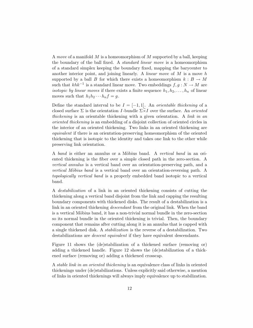
Figure 11 shows the (de)stabilization of a thickened surface (removing or)adding a thickened handle. Figure 12 shows the (de)stabilization of a thick-ened surface (removing or) adding a thickened crosscap.

A stable link in an oriented thickening is an equivalence class of links in orientedthickenings under (de)stabilizations. Unless explicitly said otherwise, a mentionof links in oriented thickenings will always imply equivalence up to stabilization.

12

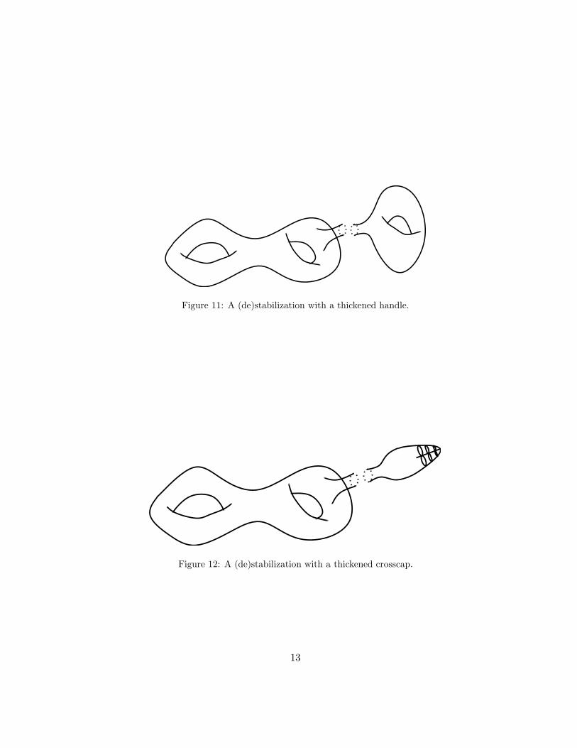
Figure 11: A (de)stabilization with a thickened handle.

Figure 12: A (de)stabilization with a thickened crosscap.

13

A surface projection of a link in an oriented thickening is a regular projection ofthe link by the bundle projection on the zero-section of the oriented thickening.The components of a surface projection are oriented by the components of thelink. Let τ, τ be unit vectors at a double point each tangent to different partsof the curve through the double point, and that agree with the orientation ofthe part to which they are tangent. A resolution of a double point of a surfaceprojection is an assignment of unit vectors η, η from the normal bundle to thesurface at the double point such that η = −η . Figure 13 shows the resolution

η

η

τ

τ

Figure 13: Resolving a double point of a surface projection.

of a double point. Then, the writhe w at a double point of a generic immersionis w = (τ × τ) · η = (τ × τ) · η .

We now consider generic immersions of oriented curves in compact surfaces asin [1]. Let τ, τ be unit vectors at a double point each tangent to different partsof the curve through the double point, and that agree with the orientationof the part to which they are tangent. A separation of a double point of ageneric immersion is an assignment of unit vectors ω, ω at the double pointsuch that ω = ±τ, ω = ±τ and such that τ · ω = τ · ω . Then, the writhe w ata double point of a generic immersion is w = τ · ω . A link surface diagram isa generic immersion with a separation of each double point. Figure 14 shows alink surface diagram for the onefoil in a Klein bottle with the short fat arrowsindicating the separation, in which case, the crossing has -1 writhe. As willbe shown later separations of double points define resolutions of the doublepoints once the surface is given an oriented thickening. And unlike the usualover-under knot diagram crossings, they do not need to change if the crossing isisotoped along an orientation-reversing loop in the surface. In drawings of linkdiagrams in surfaces, the separation can be indicated by the classical over–underconvention, so long as an isotopy of a crossing through an orientation-reversingpath switches the crossing.

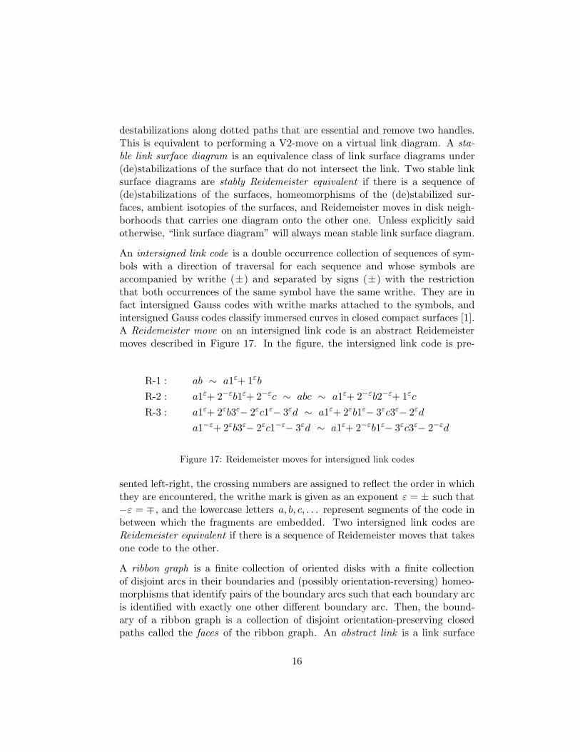
A Reidemeister move on a link surface diagram is one of the three moves il-

14

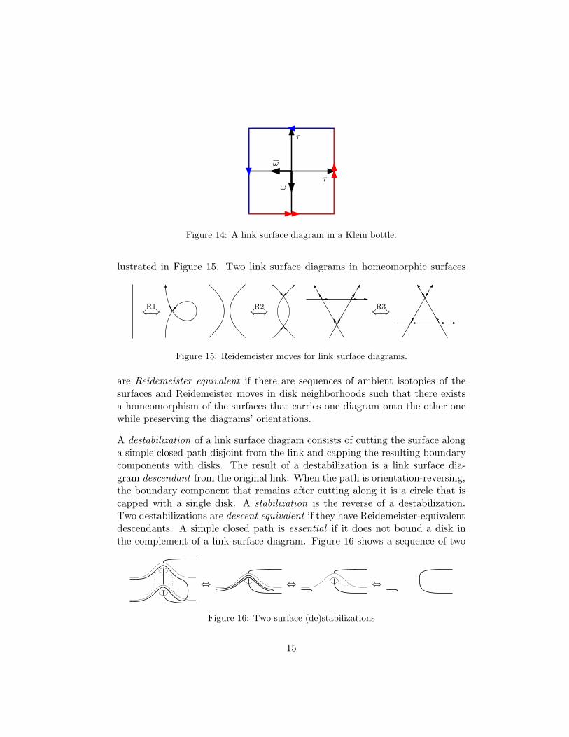
τ

ω

τ

ω

Figure 14: A link surface diagram in a Klein bottle.

lustrated in Figure 15. Two link surface diagrams in homeomorphic surfaces

R1⇐⇒

R2⇐⇒

R3⇐⇒

Figure 15: Reidemeister moves for link surface diagrams.

are Reidemeister equivalent if there are sequences of ambient isotopies of thesurfaces and Reidemeister moves in disk neighborhoods such that there existsa homeomorphism of the surfaces that carries one diagram onto the other onewhile preserving the diagrams’ orientations.

A destabilization of a link surface diagram consists of cutting the surface alonga simple closed path disjoint from the link and capping the resulting boundarycomponents with disks. The result of a destabilization is a link surface dia-gram descendant from the original link. When the path is orientation-reversing,the boundary component that remains after cutting along it is a circle that iscapped with a single disk. A stabilization is the reverse of a destabilization.Two destabilizations are descent equivalent if they have Reidemeister-equivalentdescendants. A simple closed path is essential if it does not bound a disk inthe complement of a link surface diagram. Figure 16 shows a sequence of two

⇔ ⇔ ⇔

Figure 16: Two surface (de)stabilizations

15

destabilizations along dotted paths that are essential and remove two handles.This is equivalent to performing a V2-move on a virtual link diagram. A sta-ble link surface diagram is an equivalence class of link surface diagrams under(de)stabilizations of the surface that do not intersect the link. Two stable linksurface diagrams are stably Reidemeister equivalent if there is a sequence of(de)stabilizations of the surfaces, homeomorphisms of the (de)stabilized sur-faces, ambient isotopies of the surfaces, and Reidemeister moves in disk neigh-borhoods that carries one diagram onto the other one. Unless explicitly saidotherwise, “link surface diagram” will always mean stable link surface diagram.

An intersigned link code is a double occurrence collection of sequences of sym-bols with a direction of traversal for each sequence and whose symbols areaccompanied by writhe (±) and separated by signs (±) with the restrictionthat both occurrences of the same symbol have the same writhe. They are infact intersigned Gauss codes with writhe marks attached to the symbols, andintersigned Gauss codes classify immersed curves in closed compact surfaces [1].A Reidemeister move on an intersigned link code is an abstract Reidemeistermoves described in Figure 17. In the figure, the intersigned link code is pre-

R-1 : ab ∼ a1ε+ 1εb

R-2 : a1ε+ 2−εb1ε+ 2−εc ∼ abc ∼ a1ε+ 2−εb2−ε+ 1εc

R-3 : a1ε+ 2εb3ε− 2εc1ε− 3εd ∼ a1ε+ 2εb1ε− 3εc3ε− 2εd

a1−ε+ 2εb3ε− 2εc1−ε− 3εd ∼ a1ε+ 2−εb1ε− 3εc3ε− 2−εd

Figure 17: Reidemeister moves for intersigned link codes

sented left-right, the crossing numbers are assigned to reflect the order in whichthey are encountered, the writhe mark is given as an exponent ε = ± such that−ε = ∓, and the lowercase letters a, b, c, . . . represent segments of the code inbetween which the fragments are embedded. Two intersigned link codes areReidemeister equivalent if there is a sequence of Reidemeister moves that takesone code to the other.

A ribbon graph is a finite collection of oriented disks with a finite collectionof disjoint arcs in their boundaries and (possibly orientation-reversing) homeo-morphisms that identify pairs of the boundary arcs such that each boundary arcis identified with exactly one other different boundary arc. Then, the bound-ary of a ribbon graph is a collection of disjoint orientation-preserving closedpaths called the faces of the ribbon graph. An abstract link is a link surface

16

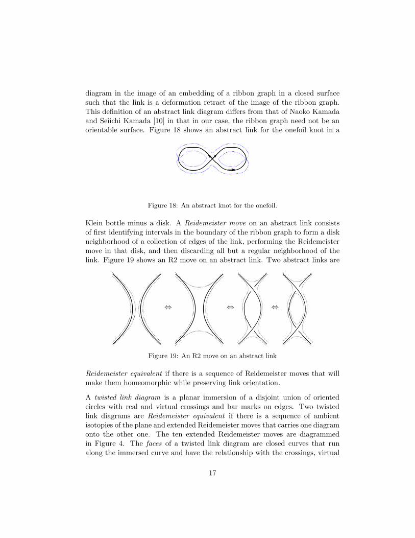
diagram in the image of an embedding of a ribbon graph in a closed surfacesuch that the link is a deformation retract of the image of the ribbon graph.This definition of an abstract link diagram differs from that of Naoko Kamadaand Seiichi Kamada [10] in that in our case, the ribbon graph need not be anorientable surface. Figure 18 shows an abstract link for the onefoil knot in a

Figure 18: An abstract knot for the onefoil.

Klein bottle minus a disk. A Reidemeister move on an abstract link consistsof first identifying intervals in the boundary of the ribbon graph to form a diskneighborhood of a collection of edges of the link, performing the Reidemeistermove in that disk, and then discarding all but a regular neighborhood of thelink. Figure 19 shows an R2 move on an abstract link. Two abstract links are

⇔ ⇔ ⇔

Figure 19: An R2 move on an abstract link

Reidemeister equivalent if there is a sequence of Reidemeister moves that willmake them homeomorphic while preserving link orientation.

A twisted link diagram is a planar immersion of a disjoint union of orientedcircles with real and virtual crossings and bar marks on edges. Two twistedlink diagrams are Reidemeister equivalent if there is a sequence of ambientisotopies of the plane and extended Reidemeister moves that carries one diagramonto the other one. The ten extended Reidemeister moves are diagrammedin Figure 4. The faces of a twisted link diagram are closed curves that runalong the immersed curve and have the relationship with the crossings, virtual

17

Figure 20: Faces and crossings, virtual crossings, and bars.

crossings, and bars as show in Figure 20. At a crossing, a face turns so as toavoid crossing the link diagram. At a virtual crossing, a face goes through thevirtual crossing. At a bar, a face crosses to the other side of the link diagram.A twisted link diagram is two-colorable if its faces can be assigned one of twocolors such that the arcs of the link diagram between two crossings alwaysseparate faces of one color from those of the other.

4 Unique Destabilization

According to Greg Kuperberg [13], links in oriented thickenings of orientableclosed surfaces have unique irreducible representatives. This is proven by show-ing that all pairs of destabilizations along essential vertical annuli are descentequivalent to destabilizations along annuli that do not intersect, and these aredescent equivalent. Theorem 1 is the equivalent statement for links in orientedthickenings over closed surfaces, and our proof will follow Kuperberg’s strategy.

Proof of Theorem 1 We expand the range of surfaces along which desta-bilizations can occur to include spheres and proper disks that separate somecomponents of the link from the other components, and bands that separatesome link-free part of the genus from the surface and so that we may discardthat part. The results of such destabilizations can be achieved by destabiliza-tions along vertical bands. In the first case, a disk or sphere may be alteredto be a band, and in the second case, the destabilization may be performedalong bands that progressively reduce genus but do not increase the number ofcomponents of the thickened surface. So we define an admissible surface to bea vertical band, sphere, or proper disk. And an admissible surface is essentialif it does not bound a ball in the complement of the link. Then, every essentialadmissible surface can be used for destabilization.

18

Let L ⊂ Σg×I = M be an n-component link in the oriented thickening of asurface Σg of Euler genus g and having c components. We require that everycomponent of M contain a part of the link, so n ≥ c.

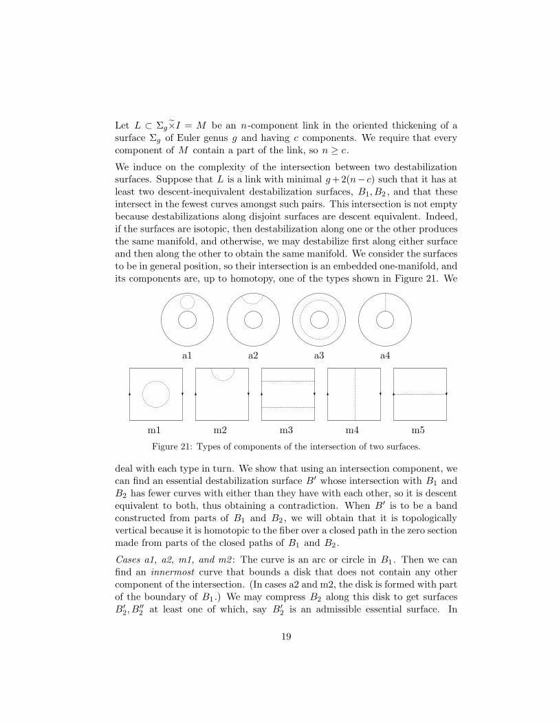
We induce on the complexity of the intersection between two destabilizationsurfaces. Suppose that L is a link with minimal g +2(n− c) such that it has atleast two descent-inequivalent destabilization surfaces, B1, B2 , and that theseintersect in the fewest curves amongst such pairs. This intersection is not emptybecause destabilizations along disjoint surfaces are descent equivalent. Indeed,if the surfaces are isotopic, then destabilization along one or the other producesthe same manifold, and otherwise, we may destabilize first along either surfaceand then along the other to obtain the same manifold. We consider the surfacesto be in general position, so their intersection is an embedded one-manifold, andits components are, up to homotopy, one of the types shown in Figure 21. We

a1 a2 a3 a4

m1 m2 m3 m4 m5

Figure 21: Types of components of the intersection of two surfaces.

deal with each type in turn. We show that using an intersection component, wecan find an essential destabilization surface B′ whose intersection with B1 andB2 has fewer curves with either than they have with each other, so it is descentequivalent to both, thus obtaining a contradiction. When B′ is to be a bandconstructed from parts of B1 and B2 , we will obtain that it is topologicallyvertical because it is homotopic to the fiber over a closed path in the zero sectionmade from parts of the closed paths of B1 and B2 .

Cases a1, a2, m1, and m2 : The curve is an arc or circle in B1 . Then we canfind an innermost curve that bounds a disk that does not contain any othercomponent of the intersection. (In cases a2 and m2, the disk is formed with partof the boundary of B1 .) We may compress B2 along this disk to get surfacesB′

2, B′′2 at least one of which, say B′

2 is an admissible essential surface. In

19

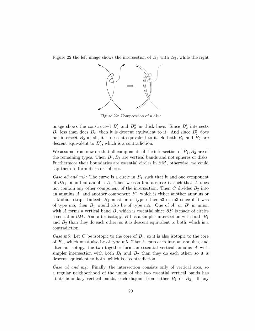
Figure 22 the left image shows the intersection of B1 with B2 , while the right

=⇒

Figure 22: Compression of a disk

image shows the constructed B′2 and B′′

2 in thick lines. Since B′2 intersects

B1 less than does B2 , then it is descent equivalent to it. And since B′2 does

not intersect B2 at all, it is descent equivalent to it. So both B1 and B2 aredescent equivalent to B′

2 , which is a contradiction.

We assume from now on that all components of the intersection of B1, B2 are ofthe remaining types. Then B1, B2 are vertical bands and not spheres or disks.Furthermore their boundaries are essential circles in ∂M , otherwise, we couldcap them to form disks or spheres.

Case a3 and m3 : The curve is a circle in B1 such that it and one componentof ∂B1 bound an annulus A. Then we can find a curve C such that A doesnot contain any other component of the intersection. Then C divides B2 intoan annulus A′ and another component B′ , which is either another annulus ora Mobius strip. Indeed, B2 must be of type either a3 or m3 since if it wasof type m5, then B1 would also be of type m5. One of A′ or B′ in unionwith A forms a vertical band B , which is essential since ∂B is made of circlesessential in ∂M . And after isotopy, B has a simpler intersection with both B1

and B2 than they do each other, so it is descent equivalent to both, which is acontradiction.

Case m5 : Let C be isotopic to the core of B1 , so it is also isotopic to the coreof B2 , which must also be of type m5. Then it cuts each into an annulus, andafter an isotopy, the two together form an essential vertical annulus A withsimpler intersection with both B1 and B2 than they do each other, so it isdescent equivalent to both, which is a contradiction.

Case a4 and m4 : Finally, the intersection consists only of vertical arcs, soa regular neighborhood of the union of the two essential vertical bands hasat its boundary vertical bands, each disjoint from either B1 or B2 . If any

20

band is essential, then it is descent equivalent to both B1 and B2 , which is acontradiction, but if none is essential, then one of them separates B1 and B2

from the link, which contradicts the fact that they are essential.

5 Twisted Link Diagrams

Theorem 2 will follow from the following lemma.

Lemma 1 There is a bijection between each of the following:

(1) Ambient isotopy equivalence classes of links in stable oriented thickenings.

(2) Reidemeister equivalence classes of link diagrams in stable surfaces.

(3) Reidemeister equivalence classes of abstract links.

(4) Reidemeister equivalence classes of twisted link diagrams.

Figure 23 illustrates the process of creating a link diagram from a link in a

⇔ ⇔ ⇔

Figure 23: Creating a diagram for a twisted link

thickened Klein bottle. The first step is a regular projection of the link tocreate a link diagram in the zero-section. The second step creates an abstractlink diagram in a regular neighborhood of the link diagram in the surface. Thethird step immerses this diagram in the plane, and decorates the result withvirtual crossings and bars.

Proof (1) ⇔ (2): Fix an oriented thickening of a closed surface and considerthe surface as the zero-section of the oriented thickening. By Sard’s theorem,the set of embeddings of a link in the manifold that have regular projectionsto the surface is dense in the set of all ambient-isotopic embeddings that forma link. The surface projection defines a resolution of the double points of theprojection as follows. Given the fiber over a neighborhood about the double

21

point, if both domain strands are on the same side of the neighborhood or onthe neighborhood, the image of the strand whose doubled point is closer to theboundary of its side has its η vector towards that boundary while the otherstrand has its η vector towards the other boundary. And if the strands are ondifferent sides, their η ’s are towards their side’s boundary. Define a separationof the surface projection from the resolution as ω = τ × η, ω = τ × η .

On the other hand, given a link surface diagram, choose an oriented thickeningof the surface. Define a resolution of the surface projection from the separationas η = ω × τ , η = ω × τ , and resolve the double point by the vectors. Ifthe thickening with the opposite orientation had been chosen, the two links inoriented thickenings are related by an orientation-preserving homeomorphism.

By Hudson and Zeeman [7], two embeddings of links in an oriented thickeningare ambient isotopic if and only if they are ambient isotopic by linear moves inarbitrary small neighborhoods. Then we may choose neighborhoods of curvessuch that their projections to the surface are generic curves whose intersectionsare in disks. Then we are in the classical case, and have that links that haveregular projections are ambient isotopic in the manifold if and only if their linksurface diagrams are Reidemeister equivalent.

There exists a destabilization of the link in oriented thickening along a topo-logically vertical band if and only if there is a destabilization of the link surfacediagram possibly preceded by a sequence of Reidemeister moves. Indeed, a ver-tical band exists as the fiber over a simple closed path in the projection surface.And if the band is only topologically vertical, it can be made vertical throughan isotopy of the link that corresponds to a sequence of Reidemeister movesbecause it is isotopic to a vertical band.

(2) ⇔ (3): Given a link surface diagram, a regular neighborhood of the link isan abstract link diagram. Given an abstract link diagram, fill in disks along itsboundary components to obtain a cellular link surface diagram, then stabilizethe surface to obtain the original link surface diagram.

Reidemeister moves on link surface diagrams are done in disk neighborhoodsobtained after stable isotopy of the link brings the strands together. And Rei-demeister moves on abstract link diagrams are done in disk neighborhoods ob-tained by bringing the strands together with homeomorphisms of the boundary.

(3) ⇔ (4): Obtain an abstract link diagram from a twisted link diagram, asfollows. Choose disk neighborhoods of the crossings in the plane. Consider thesphere S2 to be S2 × 0 ⊂ S2 × I and thicken the arcs into handles that taperto the boundaries of the disk neighborhoods. Figure 24 shows such a tapered

22

Figure 24: Arc thickened into a tapered handle.

handle between two crossings. Define arc neighborhoods in the tapered handlesby sliding an interval I from one tapered end to the other along arc such thatthe interval is always normal to the arc, and passes through the normal to S2

in S2 × I if and only if there is a bar at that point on the arc. Move the arcneighborhoods by a small amount so that they do not intersect one another intoone of the two ways shown in Figure 25. Different choices of movement of the

⇐⇒

Figure 25: Two ways to resolve a virtual crossing

arc neighborhoods and of direction of turn of the interval as it slides along thearc yield homeomorphic abstract link diagrams although it produces a differentembedding of that diagram in S2 × I .

Suppose two link diagrams differ by an extended Reidemeister move. If themove is classical, then the equivalent classical move exists on the abstract linkdiagram. If the move is virtual or twisted, then the embedding is changed insome version of what is shown in Figure 26 but the abstract link diagram isunchanged.

Obtain a twisted link diagram from an abstract link diagram as follows. Embedthe abstract link diagram in S2×I such that each crossing has a disk neighbor-hood in S2 , and that the projection of the embedding to S2 is an immersion.On the projected diagram, draw crossings in the over-under form dependingon the resolution of the abstract link crossings. Draw each intersection of two

23

V1⇐⇒

V2⇐⇒

V3⇐⇒

V4⇐⇒

T1⇐⇒

T2⇐⇒

T3⇐⇒

Figure 26: Virtual and twisted changes to embeddings.

projected arcs as a virtual crossing. Draw each inter-component intersection ofthe projection of the two boundary components of the neighborhood of eacharc as bars on the arc. Figure 27 shows the projection of an arc and the bound-

Figure 27: Arc boundary intersection giving rise to a bar

ary components, and draws one bar on the arc for the single inter-componentintersection of thee two boundary components.

Suppose two different embeddings g, g′ of the same abstract link give rise todifferent twisted link diagrams. We can change g by embedding each neighbor-hood of a crossing with the opposite rotation of the arcs to make them matchthat of g′ , which corresponds to a series of T3 moves. Figure 28 shows theeffect of performing a T3 move on both an embedding of an abstract link andon the corresponding twisted link diagram. We can change g by an isotopy ofS2 to make its neighborhoods of crossings including the arcs correspond to that

24

⇔

⇔

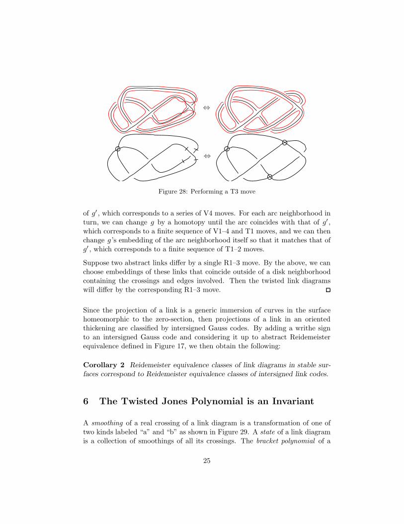
Figure 28: Performing a T3 move

of g′ , which corresponds to a series of V4 moves. For each arc neighborhood inturn, we can change g by a homotopy until the arc coincides with that of g′ ,which corresponds to a finite sequence of V1–4 and T1 moves, and we can thenchange g ’s embedding of the arc neighborhood itself so that it matches that ofg′ , which corresponds to a finite sequence of T1–2 moves.

Suppose two abstract links differ by a single R1–3 move. By the above, we canchoose embeddings of these links that coincide outside of a disk neighborhoodcontaining the crossings and edges involved. Then the twisted link diagramswill differ by the corresponding R1–3 move.

Since the projection of a link is a generic immersion of curves in the surfacehomeomorphic to the zero-section, then projections of a link in an orientedthickening are classified by intersigned Gauss codes. By adding a writhe signto an intersigned Gauss code and considering it up to abstract Reidemeisterequivalence defined in Figure 17, we then obtain the following:

Corollary 2 Reidemeister equivalence classes of link diagrams in stable sur-

faces correspond to Reidemeister equivalence classes of intersigned link codes.

6 The Twisted Jones Polynomial is an Invariant

A smoothing of a real crossing of a link diagram is a transformation of one oftwo kinds labeled “a” and “b” as shown in Figure 29. A state of a link diagramis a collection of smoothings of all its crossings. The bracket polynomial of a

25

a⇒ or

b⇒

Figure 29: Two possible smoothings of a crossing.

link diagram D is an element of Z[A±1,M ] defined from the possible statesS(D) of D by:

〈D〉 =∑

S∈S(D)

Aa(S)−b(S)(−A−2 − A2)c(S)Md(S)

where:

• a(S) is the number of a-smoothings,

• b(S) is the number of b-smoothings,

• c(S) is the number of circles with an even number of bars, and

• d(S) is the number of circles with an odd number of bars.

The twisted Jones polynomial of a link diagram D is an element of Z[A±1,M ]calculated as:

VD(A,M) = (−A)−3w(D) 〈D〉 .

We prove that the extension to the Jones polynomial defined above is an in-variant of links in oriented thickenings, and that it distinguishes a class of linksin oriented thickenings from virtual links.

Proof of Theorem 3 The bracket polynomial of link diagrams in orientedthickenings is equivalent to that defined by the relations:

(1) 〈∅〉 = 1,

(2)

⟨ ⟩= A

⟨ ⟩+ A−1

⟨ ⟩,

(3)

⟨D ∐

⟩= (−A−2 − A2) 〈D〉,

(4)

⟨D ∐

⟩= M 〈D〉,

26

(5)

⟨ ⟩=

⟨ ⟩.

This can be seen by first using relation 2 to smooth the crossings of a diagramD in all possible ways, so that each final diagram of circles corresponding to oneof the states of D . Then, relation 5 allows each circle to be reduced to either0 or 1 bars. Finally, the other relations allow the calculation of the bracketpolynomial.

Invariance with respect to R1–3 and V1–4 is immediately due to that of theJones polynomial. Invariance with respect to T1 is immediate since it involvesno real crossings. Invariance with respect to T2 is shown by relation 5. Then,the twisted Jones polynomial is invariant with respect to move T3 by the cal-culation:

⟨ ⟩= A

⟨ ⟩+ A−1

⟨ ⟩by (2)

= A

⟨ ⟩+ A−1

⟨ ⟩by (T1)

= A

⟨ ⟩+ A−1

⟨ ⟩by (V1,V2)

=

⟨ ⟩. by (2)

So the twisted Jones polynomial is an invariant of links in oriented thickenings.

Since virtual links do not have bars on their edges, then their states will not haveany circles with an odd number of bars, and so their twisted Jones polynomialswill be in Z[A±1]. And since the (−A−2 − A2) term is raised to the numberof circles in a state, the twisted Jones polynomial will factor into a product of(−A−2 − A2) and the Jones polynomial of the diagram.

The Jones polynomial can be extended to links in oriented thickenings by thedevice of ignoring bars on edges. This invariant corresponds to setting M =−A−2 −A2 in the new polynomial and then dividing the result by −A−2 −A2 .

The onefoil shown in Figure 3 has twisted Jones polynomial:

VOnefoil(A,M) = A−6 + (1 − M2)A−2

so it is not a virtual knot.

27

7 Twisted Jones of Two-Colorable Diagrams

The knot K in Figure 6 has twisted Jones polynomial:

VK(A,M) = (−A−2 − A2)(A−4 + A−6 − A−10)

which is a product of (−A−2 − A2) and of the Jones polynomial for the knot.But this knot is in the projective plane and cannot be moved to an affine subsetof this space, so it is not a classical knot [3]. We will see that the knot’s twistedJones polynomial factors in this manner because it has a two-colorable diagram.

Proof of Theorem 4 Let D be a two-colored diagram for a link. This two-coloring partitions the faces of D into two sets of circles each of one of thetwo colors and such that each crossing of the diagram will separate a diskneighborhood of that crossing into two pairs of regions that are opposite oneanother with respect to the crossing and that contain like-colored parts of thefaces of the diagram. Figure 30 shows this situation for an arbitrary crossing.

Figure 30: A crossing of a two-colored diagram

In the figure, the parts of faces are drawn either dotted or dashed to representthe two colors while the boundary of the disk is drawn with a dash-dot-dottedpattern. The two possible smoothings of each crossing of a diagram also pairopposite regions of the crossing. In the figure, the dashed lines are the “a”smoothing while the dotted lines are the “b” smoothing. Then, the faces ofone color of D are the circles of the state of D whose smoothings pair thecorresponding two opposite regions of each crossing, and the faces of the othercolor are the circles of the complementary state of D . Since the circles of eachof these states correspond to faces of a diagram and that by the Jordan curvetheorem the faces cross the link diagram an even number of times at bars, thenthe circles have an even number of bars.

28

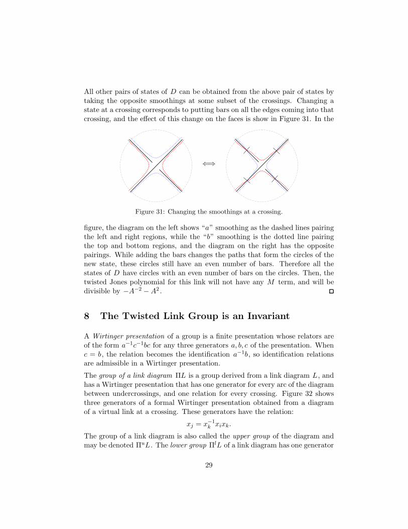
All other pairs of states of D can be obtained from the above pair of states bytaking the opposite smoothings at some subset of the crossings. Changing astate at a crossing corresponds to putting bars on all the edges coming into thatcrossing, and the effect of this change on the faces is show in Figure 31. In the

⇐⇒

Figure 31: Changing the smoothings at a crossing.

figure, the diagram on the left shows “a” smoothing as the dashed lines pairingthe left and right regions, while the “b” smoothing is the dotted line pairingthe top and bottom regions, and the diagram on the right has the oppositepairings. While adding the bars changes the paths that form the circles of thenew state, these circles still have an even number of bars. Therefore all thestates of D have circles with an even number of bars on the circles. Then, thetwisted Jones polynomial for this link will not have any M term, and will bedivisible by −A−2 − A2 .

8 The Twisted Link Group is an Invariant

A Wirtinger presentation of a group is a finite presentation whose relators areof the form a−1c−1bc for any three generators a, b, c of the presentation. Whenc = b, the relation becomes the identification a−1b, so identification relationsare admissible in a Wirtinger presentation.

The group of a link diagram ΠL is a group derived from a link diagram L, andhas a Wirtinger presentation that has one generator for every arc of the diagrambetween undercrossings, and one relation for every crossing. Figure 32 showsthree generators of a formal Wirtinger presentation obtained from a diagramof a virtual link at a crossing. These generators have the relation:

xj = x−1k xixk.

The group of a link diagram is also called the upper group of the diagram andmay be denoted ΠuL. The lower group ΠlL of a link diagram has one generator

29

xj xi

xk

Figure 32: Generators at a crossing for a formal presentation

for every arc of the diagram between overcrossings, and again one relation forevery crossing defined analogously to that of the upper group.

The twisted link group of a diagram ΠL is a group with a Wirtinger presen-tation that has two generators for each side of each end of an edge. Figure 33shows eight generators obtained from a diagram of a link at a crossing. These

xi xi

xi+1 xi+1

xj+1

xj+1

xj

xj

Figure 33: Generators at a crossing for a twisted presentation

generators have the four crossing relations:

xi+1 = xi, xj+1 = x−1i xjxi,

xi+1 = x−1j xixj , xj+1 = xj .

The four generators of an edge have two relations depending on the parity ofthe number of bars on the edge. Figure 34 shows the four generators of an edge.When an edge has an even number of bars between two crossings, we have therelations:

xi+1 = xi, xi+1 = xi,

30

xi

xi+1

xi

xi+1

Bars

Figure 34: Generators on an edge for a twisted presentation

and when there is an odd number of bars on the arc, we have the relations:

xi+1 = xi, xi+1 = xi.

Proof of Theorem 5 Note that performing moves V1–4 and T1–2 on a linkdiagram yield a link diagram with an identical presentation. Invariance withrespect to moves R1–3 is the same as for classical link diagrams since neithervirtual crossings nor bars are involved. Finally, invariance with respect to T3is as follows. Figure 35 shows half of the generators on the edges of the two

xi

xi−1

xi+1

xi+2

xj

xj−1

xj+1

xj+2

T3⇐⇒

xi−1

xi

xi+1

xi+2

xj−1

xj

xj+1

xj+2

Figure 35: The generators in move T3.

diagrams. Then, the relations given by the crossing are:

On the left On the right

x−1j+1x

−1i xjxi x−1

j+1x−1i xjxi

x−1i+1xi x−1

i+1xi

31

which are identical. Doing the same for the other half of the generators showsthe corresponding equivalence.

References

[1] M Bourgoin, Classifying Immersed Curves, in Preparation

[2] M Bourgoin, On the Fundamental Group of a Virtual Link, in Preparation

[3] Yu V Drobotukhina, An analogue of the Jones polynomial for links in RP3

and a generalization of the Kauffman-Murasugi theorem, Algebra i Analiz 2(1990) 171–191

[4] Yu V Drobotukhina, Classification of projective Montesinos links, Algebra iAnaliz 3 (1991) 118–130

[5] Yu V Drobotukhina, Classification of links in RP3 with at most six cross-ings [MR 93b:57006], from: “Topology of manifolds and varieties”, Adv. SovietMath. 18, Amer. Math. Soc., Providence, RI (1994) 87–121

[6] Jonathan L Gross, Thomas W Tucker, Topological graph theory, Wiley-Interscience Series in Discrete Mathematics and Optimization, John Wiley &Sons Inc., New York (1987), a Wiley-Interscience Publication

[7] J F P Hudson, E C Zeeman, On combinatorial isotopy, Inst. Hautes EtudesSci. Publ. Math. (1964) 69–94

[8] Vaughan F R Jones, A polynomial invariant for knots via von Neumann al-gebras, Bull. Amer. Math. Soc. (N.S.) 12 (1985) 103–111

[9] Naoko Kamada, On the Jones polynomials of checkerboard colorable virtuallinks, Osaka J. Math. 39 (2002) 325–333

[10] Naoko Kamada, Seiichi Kamada, Abstract link diagrams and virtual knots,J. Knot Theory Ramifications 9 (2000) 93–106

[11] Louis H Kauffman, State models and the Jones polynomial, Topology 26(1987) 395–407

[12] Louis H Kauffman, Virtual knot theory, European J. Combin. 20 (1999) 663–690

[13] Greg Kuperberg, What is a virtual link?, Algebr. Geom. Topol. 3 (2003)587–591 (electronic), math.GT/0208039

[14] Maciej Mroczkowski, Diagrammatic unknotting of knots and links in the pro-jective space, J. Knot Theory Ramifications 12 (2003) 637–651

[15] Maciej Mroczkowski, Polynomial invariants of links in the projective space,Fund. Math. 184 (2004) 223–267

[16] Sam Nelson, Unknotting virtual knots with Gauss diagram forbidden moves,J. Knot Theory Ramifications 10 (2001) 931–935

32

[17] Daniel S Silver, Susan G Williams, Virtual knot groups, from: “Knots inHellas ’98 (Delphi)”, Ser. Knots Everything 24, World Sci. Publishing, RiverEdge, NJ (2000) 440–451

Department of Mathematics

Brandeis University

Waltham, MA 02454

Email: [email protected]

33

Twisted Link Theory

Documents

Transcript of Twisted Link Theory