Twisted Extensions of Fermat's Last Theorem - Open Collections
299
. Twisted Extensions of Fermat’s Last Theorem by Carmen Anthony Bruni A thesis submitted in partial fulfillment of the requirements for the degree of Doctor of Philosophy in The Faculty of Graduate and Postdoctoral Studies (Mathematics) The University of British Columbia (Vancouver) April 2015 c Carmen Anthony Bruni, 2015
-
Upload
khangminh22 -
Category
Documents
-
view
1 -
download
0
Transcript of Twisted Extensions of Fermat's Last Theorem - Open Collections

.
Twisted Extensions of Fermat’s Last Theorem
by
Carmen Anthony Bruni
A thesis submitted in partial fulfillment of the requirements for
the degree of
Doctor of Philosophy
in
The Faculty of Graduate and Postdoctoral Studies
(Mathematics)
The University of British Columbia
(Vancouver)
April 2015
c© Carmen Anthony Bruni, 2015

Abstract
Let x, y, z, p, n, α ∈ Z with α ≥ 1, p and n ≥ 5 primes. In 2011, Michael Bennett, Florian
Luca and Jamie Mulholland showed that the equation x3+y3 = pαzn has no pairwise coprime
nonzero integer solutions provided p ≥ 5, n ≥ p2p and p /∈ S where S is the set of primes q
for which there exists an elliptic curve of conductor NE ∈ 18q, 36q, 72q with at least one
nontrivial rational 2-torsion point. In this thesis, I will present a solution that extends the
result to include a subset of the primes in S; those q ∈ S for which all curves with conductor
NE ∈ 18q, 36q, 72q with nontrivial rational 2-torsion have discriminants not of the form `2
or −3m2 with `,m ∈ Z. Using a similar approach, I will classify certain integer solutions to
the equation x5 +y5 = pαzn which in part generalizes work done from Billerey and Dieulefait
in 2009. I will also discuss limitations of the methods for these equations and as they extend
to further prime exponents.
ii

Preface
This dissertation is original, unpublished, independent work by the author, Carmen An-
thony Bruni.
iii

.
.
Table of Contents
Abstract . . . . . . . . . . . . . . . . . . . . . . . . . . . . . . . . . . . . . . . . . . ii
Preface . . . . . . . . . . . . . . . . . . . . . . . . . . . . . . . . . . . . . . . . . . . iii
Table of Contents . . . . . . . . . . . . . . . . . . . . . . . . . . . . . . . . . . . . iv
List of Tables . . . . . . . . . . . . . . . . . . . . . . . . . . . . . . . . . . . . . . . vi
Acknowledgements . . . . . . . . . . . . . . . . . . . . . . . . . . . . . . . . . . . viii
Dedication . . . . . . . . . . . . . . . . . . . . . . . . . . . . . . . . . . . . . . . . . x
1 Introduction . . . . . . . . . . . . . . . . . . . . . . . . . . . . . . . . . . . . . . 1
1.1 The History of the Problem . . . . . . . . . . . . . . . . . . . . . . . . . . . 1
1.2 Elliptic Curves . . . . . . . . . . . . . . . . . . . . . . . . . . . . . . . . . . 4
1.3 Modular Forms . . . . . . . . . . . . . . . . . . . . . . . . . . . . . . . . . . 14
1.4 A Modern Approach to Fermat’s Last Theorem . . . . . . . . . . . . . . . . 17
1.5 Where Do Frey-Hellegouarch Curves Come From? . . . . . . . . . . . . . . . 22
1.6 Ternary Fermat-Type Diophantine Equations . . . . . . . . . . . . . . . . . 26
1.7 Results From This Thesis . . . . . . . . . . . . . . . . . . . . . . . . . . . . 29
2 Classification of Elliptic Curves With Nontrivial Rational Two Torsion 31
2.1 On the Q-Isomorphism Classes of Elliptic Curves With Nontrivial Rational
2-Torsion and Conductor 2LqMpN . . . . . . . . . . . . . . . . . . . . . . . . 31
2.2 Elliptic Curves With Nontrivial Rational Two Torsion and Conductor 2aqbpc 35
3 Diophantine Equations . . . . . . . . . . . . . . . . . . . . . . . . . . . . . . . 131
3.1 S-Integer Solutions to y2 = x3 ± 2α5β . . . . . . . . . . . . . . . . . . . . . . 131
3.2 Integer and Rational Solutions to y2 = x5 ± 2α5β . . . . . . . . . . . . . . . 136
3.2.1 Chabauty’s Method . . . . . . . . . . . . . . . . . . . . . . . . . . . . 136
3.2.2 Elliptic Curve Chabauty . . . . . . . . . . . . . . . . . . . . . . . . . 147
3.2.3 S-integer Points . . . . . . . . . . . . . . . . . . . . . . . . . . . . . . 153
iv

3.2.4 Other Techniques . . . . . . . . . . . . . . . . . . . . . . . . . . . . . 157
3.2.5 Integer Points Via Thue-Mahler Equations . . . . . . . . . . . . . . . 157
3.3 Other Results . . . . . . . . . . . . . . . . . . . . . . . . . . . . . . . . . . . 178
3.4 Diophantine Equations Relating to Elliptic Curves . . . . . . . . . . . . . . . 180
4 Elliptic Curves With Rational Two Torsion and Conductor 18p, 36p or
72p Organized by Primes . . . . . . . . . . . . . . . . . . . . . . . . . . . . . . 213
5 Elliptic Curves With Rational Two Torsion and Conductor 50p, 200p or
400p Organized by Primes . . . . . . . . . . . . . . . . . . . . . . . . . . . . . 235
6 On the Diophantine Equation x5 + y5 = pαzn . . . . . . . . . . . . . . . . . . 254
7 Strengthening Results on the Diophantine Equation xq + yq = pαzn . . . . 263
Bibliography . . . . . . . . . . . . . . . . . . . . . . . . . . . . . . . . . . . . . . . 278
Appendix A Final Collection of Tables . . . . . . . . . . . . . . . . . . . . . . . 288
v

.
.
List of Tables
2.1 Elliptic curves of conductor 2LqMpN when a4 > 0 . . . . . . . . . . . . . . . 34
2.2 Elliptic curves of conductor 2LqMpN when a4 < 0 . . . . . . . . . . . . . . . 35
3.1 Integer solutions to y2 = x3 + 2α5β with x-coordinate 2ApB, p 6= 2, 5 , B ≥ 1
and A,α, β ≥ 0. . . . . . . . . . . . . . . . . . . . . . . . . . . . . . . . . . . 133
3.2 Integer solutions to y2 = x3 + 2α5β with x-coordinate 5ApB, p 6= 2, 5 , B ≥ 1
and A,α, β ≥ 0. . . . . . . . . . . . . . . . . . . . . . . . . . . . . . . . . . . 133
3.3 Integer solutions to y2 = x3 + 2α5β with x-coordinate 2A5BpC , p 6= 2, 5, C ≥ 1
and A,B, α, β ≥ 0. . . . . . . . . . . . . . . . . . . . . . . . . . . . . . . . . 134
3.4 Integer solutions to y2 = x3− 2α5β with x-coordinate pA, p 6= 2, 5 , A ≥ 1 and
α, β ≥ 0. . . . . . . . . . . . . . . . . . . . . . . . . . . . . . . . . . . . . . . 134
3.5 Integer solutions to y2 = x3 − 2α5β with x-coordinate 2ApB, p 6= 2, 5 , B ≥ 1
and A,α, β ≥ 0. . . . . . . . . . . . . . . . . . . . . . . . . . . . . . . . . . . 135
3.6 Integer solutions to y2 = x3 − 2α5β with x-coordinate 5ApB, p 6= 2, 5 , B ≥ 1
and A,α, β ≥ 0. . . . . . . . . . . . . . . . . . . . . . . . . . . . . . . . . . . 135
3.7 Integer solutions to y2 = x3− 2α5β with x-coordinate 2A5BpC , p 6= 2, 5, C ≥ 1
and A,B, α, β ≥ 0. . . . . . . . . . . . . . . . . . . . . . . . . . . . . . . . . 136
3.8 Rational solutions to y2 = x5 + 2α5β. . . . . . . . . . . . . . . . . . . . . . . 137
3.9 Rational solutions to y2 = x5 − 2α5β. . . . . . . . . . . . . . . . . . . . . . . 138
3.10 Rational solutions to y2 = x5 + 2α5β for rank 0 curves . . . . . . . . . . . . . 142
3.11 Rational points on y2 = x5 + 2α5β for known rank 1 curves. . . . . . . . . . . 146
3.12 Rational points on y2 = x5 − 2α5β for known rank 1 curves. . . . . . . . . . . 147
3.13 Rational solutions to y2 = x5 ± 2α5β solved using Elliptic Curve Chabauty. . 153
3.14 Solutions to gj(m,n) = ±2δ15δ2 with gcd(m,n) = 1 and n coprime to the
coefficient of gj(m, 0). . . . . . . . . . . . . . . . . . . . . . . . . . . . . . . . 161
3.15 Solutions to fk(m,n) = 2δ15δ2 with gcd(m,n) = 1 and n coprime to the
coefficient of gj(m, 0). . . . . . . . . . . . . . . . . . . . . . . . . . . . . . . . 162
3.16 Solutions to gj(m,n) = ±2δ15δ2 with gcd(m,n) = 1 and n coprime to the
coefficient of gj(m, 0). . . . . . . . . . . . . . . . . . . . . . . . . . . . . . . . 163
vi
3.17 Solutions to fk(m,n) = 2δ15δ2 with gcd(m,n) = 1 and n coprime to the
coefficient of gj(m, 0). . . . . . . . . . . . . . . . . . . . . . . . . . . . . . . . 164
3.18 Solutions to gj(m,n) = ±2δ15δ2 with gcd(m,n) = 1 and n coprime to the
coefficient of gj(m, 0). . . . . . . . . . . . . . . . . . . . . . . . . . . . . . . . 166
3.19 Solutions to fk(m,n) = 2δ15δ2 with gcd(m,n) = 1 and n coprime to the
coefficient of gj(m, 0). . . . . . . . . . . . . . . . . . . . . . . . . . . . . . . . 167
3.20 Integer solutions to x2 + 2α5β = yn with x, y ≥ 1, gcd(x, y) = 1 and n ≥ 3
with α, β > 0. . . . . . . . . . . . . . . . . . . . . . . . . . . . . . . . . . . . 199
3.21 Summary of solutions with n ≥ 1, ` = 2 or ` ≥ 4 and m ≥ 0 for the equation
d2 + 2`5mpn = ε. . . . . . . . . . . . . . . . . . . . . . . . . . . . . . . . . . . 210
3.22 Summary of solutions with n ≥ 1, ` = 2 or ` ≥ 4 and m ≥ 0 for the equation
d2 + δ2`pn = ε5m. . . . . . . . . . . . . . . . . . . . . . . . . . . . . . . . . . 210
3.23 Summary of solutions with n ≥ 1, ` = 2 or ` ≥ 4 and m ≥ 0 for the equation
d2 + δ2`5m = εpn. . . . . . . . . . . . . . . . . . . . . . . . . . . . . . . . . . 211
3.24 Summary of solutions with n ≥ 1, ` = 2 or ` ≥ 4 and m ≥ 0 for the equation
d2 + δ2` = ε5mpn. . . . . . . . . . . . . . . . . . . . . . . . . . . . . . . . . . 211
3.25 Summary of solutions with n ≥ 1, ` = 2 or ` ≥ 4 and m ≥ 0 for the equation
5d2 − 2`pn = ε. . . . . . . . . . . . . . . . . . . . . . . . . . . . . . . . . . . 212
3.26 Summary of solutions with n ≥ 1, ` = 2 or ` ≥ 4 and m ≥ 0 for the equation
5d2 − δ2` = εpn. . . . . . . . . . . . . . . . . . . . . . . . . . . . . . . . . . . 212
7.1 Primes not in Pg,3. . . . . . . . . . . . . . . . . . . . . . . . . . . . . . . . . 267
7.2 Primes not in Pg,5. . . . . . . . . . . . . . . . . . . . . . . . . . . . . . . . . 268
7.3 Primes not in Pb,3 but in Pg,3. . . . . . . . . . . . . . . . . . . . . . . . . . . 270
7.4 Primes not in Pb,5 but in Pg,5. . . . . . . . . . . . . . . . . . . . . . . . . . . 271
7.5 Remaining primes for q = 3. . . . . . . . . . . . . . . . . . . . . . . . . . . . 272
7.6 Remaining primes for q = 5. . . . . . . . . . . . . . . . . . . . . . . . . . . . 273
A.1 Primes p of Pg,3 with p ≤ 1800 . . . . . . . . . . . . . . . . . . . . . . . . . . 288
A.2 Primes p of Pb,3 with p ≤ 1800 . . . . . . . . . . . . . . . . . . . . . . . . . . 289
A.3 Primes p of Pg,5 with p ≤ 320 . . . . . . . . . . . . . . . . . . . . . . . . . . 289
A.4 Primes p of Pb,5 with p ≤ 320 . . . . . . . . . . . . . . . . . . . . . . . . . . 289
vii

Acknowledgements
My sincerest and utmost thanks to my supervisor Professor Michael Bennett for all of his
patience and dedication to me as a Ph.D. student. I cannot express in words how much it
has meant to have someone who has believed in me as much as you have over the years. Your
guidance and help has made this project possible. I am very thankful to have a supervisor
with your vision and expertise in the field.
To my supervisory committee Professors Greg Martin and Vinayak Vatsal, thank you
so much for always being available for advice and for teaching. It has been great having a
committee with such a kind and generous open door policy. Your guidance has always been
appreciated over the years!
I would also like to thank many professors I have had discussions with including Professors
Nils Bruin, Samir Siksek and Michael Stoll. A thank you as well to the many people who
reply to MathOverflow posts.
I would also like to thank the faculty and staff at the University of British Columbia,
especially all the support staff in Math 121. Over the years I have spoken to just about
everyone in that room and their knowledge of the hidden working of a university is so in-
valuable. The University of British Columbia is very blessed to have such a great room of
people.
A big thank you goes out to all of my friends and family back at home who have supported
me over the years. I would like to especially thank my parents for supporting me over these
last 10 years both emotionally and mentally with the highs and lows that come with a
graduate degree. Without such a loving and supportive family cast I’m not sure how this
would have been possible.
To my fiancee Jessica. I cannot put into words how much your love and support has
meant to me over these last 5 years of my degree. Thank you so much for always being
there to help me. Thank you for picking me up when I was down and reminding me to stay
healthy when I was too busy to remember. Thanks for helping me to explore Vancouver and
viii

reminding me that there is so much more to life than mathematics. Thank you for being
there in the past and thank you in advance for being there in the future.
To my friends from Waterloo, especially Vince and Vicki Chan and Faisal al-Faisal. Over
the last 10 years you have been my go to people for help and advice for all things math
related. Thank you for being a part of my life. This project could not have been successful
without such a great group of core friends.
To my friends here at the University of British Columbia, thank you for everything. I
could state the names of about half the math graduate students by now over the last 5 years
here but let me just keep it short and say that you know who you are and thank you so
much for helping me to keep my sanity intact. A big thank you especially to my office mates
in Math 201 and to the MER wiki team for always being there when the stress of graduate
school was too much for me to handle alone.
Finally I would like to acknowledge that this project was funded in part by both a CGS-M
scholarship and a Four Year Fellowship from the University of British Columbia for which I
am thankful for.
ix

Dedication
Per mia nonna Giuseppina Mattina e mia zia Carmela Mattina. Il vostro amore e il duro
lavoro ha reso possibile questa tesi. Che tu possa riposare in pace con il comfort di Dio.
x

Chapter 1
Introduction
1.1 The History of the Problem
A Diophantine equation is a polynomial defined over Z[x1, .., xn] where we seek out integer
(or rational) n-tuples satisfying the polynomial. These equations are named after Diophantus
of Alexandria who lived during the third century A.D. His book Arithmetica contains such
equations which he solved for using positive rational numbers. For a more thorough view of
the history of Diophantus, see [Sch98]1.
Throughout the last 2600 years of number theory, a great deal of mathematics has been
created to solve Diophantine equations. Some of the earliest attempts at solving Diophantine
equations date back to Pythagoreas. He was particularly interested in the equation x2 +y2 =
z2. This equation is the Pythagorean theorem for right angled triangles, which geometrically
says that sum of the squares of the perpendicular sides of a triangle equals the square of its
hypotenuse. A question one can ask is “Which right angled triangles have all integer side
lengths?” With a bit of effort, we can come up with a few simple examples, the most well
known being (3, 4, 5) and (5, 12, 13) and then notice that integer multiples of these will also
work such as (6, 12, 15) or (2500, 6000, 6500). In light of this, we call a solution primitive
if there is no common multiple between the three variables. Simplifying our question, we
now ask “Can we find all such primitive solutions?” This question at first might seem ill
posed - what happens if there are infinitely many? One cannot list all solutions if there
are infinitely many. In this case, what we can hope to find is a parameterized family of
solutions, that is, equations for the variables that depend on parameters in such a way that
if we replace the parameters with integers, we get solutions to our original equation and that
these solutions form a comprehensive list. It is said that Pythagoreas was the first to attempt
1An English translation can be found on the author’s personal webpage at 〈http://www-irma.u-strasbg.fr/~schappa/NSch/Publications_files/Dioph.pdf〉.
1

such a parameterization and came up with the following [Ito87]
(x, y, z) = (2n+ 1, 2n2 + 2n, 2n2 + 2n+ 1)
for a (positive) integer n. This parameterization gives an infinite family of solutions, but not
a complete list. The full parameterization is possible and is given by
(x, y, z) = (s2 − t2, 2st, s2 + t2)
where s and t are integers. This was first given in Euclid Elements [Euc02, Book 10 Propo-
sition 29].
From here, it seems like a simple switch would be to turn all the squares into cubes, that
is to examine the equation x3 + y3 = z3. Thinking about this geometrically, we are asking
can we write the volume of a cube as the sum of two volumes of cubes. There are some trivial
such examples of this problem, namely when one of the cubes has 0 length so we further say
that a solution to a Diophantine equation is trivial if xyz = 0, that is, if at least one of the
components is zero. Now as before, we ask “Can we classify all non-trivial primitive solutions
to this equation?” This question can be resolved in the affirmative. It is known that no such
solutions exist, the first proof of which was given formally by Leonhard Euler in 1770. He
used the method of infinite descent, the same method that Pierre de Fermat used to solve
the case of x4 + y4 = z4 in the 1600s [Bal60, p.242]. Fermat seldom formally published any
of his proofs however stories say that whenever asked for a proof, he could always produce
one [Bal60, p.242].
This brings us to our title character, Pierre de Fermat. In the margin of his copy of
Diophantus’ Arithmetica2, he wrote down, after translating to modern language, that the
equation xn + yn = zn had no non-trivial primitive solutions and claimed he had a remark-
able proof of this fact for which the margin was too narrow to contain. Since that time,
mathematicians have sought out a solution to this problem. This quest as we will see took
many years before being completed.
Years later, in 1847, Gabriel Lame announced a proof of Fermat’s Last Theorem using
the idea of cyclotomic numbers [Dev90, p.278]. Let p ≥ 5 be a prime number and let ζp be a
primitive pth root of unity, that is, a strictly complex solution to xp − 1. Lame argues that
2The term “Diophantine equation” originates from the name Diophantus.
2

if (x, y, z) is a solution to Fermat’s Last Theorem with exponent p a prime, then
zp = xp + yp =
p−1∏i=0
(x+ ζ ipy)
and then one argues that each (x + ζ ipy) is a pth power times a unit. Argue similarly for
xp + (−z)p and then use these two pieces of information to derive a contradiction (see [BS66,
Chapter 3] for the full and complete argument). The problem with this proof is that three
years earlier, Ernst Kummer showed that the ring Z[ζ23] fails to be a unique factorization
domain. In one sentence, the elements of this ring do not behave like integers in the sense that
elements do not necessarily decompose into a product of prime elements uniquely, contrary
to how the Fundamental Theorem of Arithmetic works for the integers. This failure prevents
each factor in the product above from necessarily being a pth power as Lame assumes.
Kummer in 1847 found a way around this. He introduced the idea of using ideals to attempt
to solve this problem. Over prime ideals, unique factorization does occur as we know it and
much of the theory of integers carries through. The concept of the class number, the size of
the group of fractional ideals modulo the principal fractional ideals, has its roots here. He
shows that if the prime p does not divide the order of this finite group, then the Fermat
equation for exponent p has only trivial solutions. These primes are called regular primes
and Kummer showed that the only primes less than 100 that are not regular are 37, 59 and
67.
Seeing just how close Kummer was to a proof, it seemed that a solution would soon
surface. Sadly this is not the case. The next big step towards solving Fermat’s Last Theorem
is due to Louis Mordell. In 1922, Mordell noticed that when dealing with a Diophantine
equation, there were no known examples of equations of genus (an algebraic invariant of the
equation) bigger than or equal to 2 where the number of rational points was infinite [Dev90,
p.286]. He conjectured that if one considers an equation with genus strictly bigger than 1,
then the equation in question must only have finitely many primitive integer solutions. It
was not until 1983 when Gerd Faltings proved that indeed this is true [Fal83]. For his work,
he was awarded the Fields Medal in 1986.
Now Plucker’s formula says that for n ≥ 4, the genus of the curve xn + yn = zn is at
least 2. Hence, we know that each such curve has only finitely many primitive integer points.
Unfortunately, Faltings’ theorem is not effective meaning that while you know that there
are only finitely many solutions, the theorem does not give you an algorithm on how to find
them. The statement that we wish to prove is that the equation xn+yn = zn has only trivial
primitive solutions and up to this point in time, we are close, but still far away.
3

This brings us to the work of Andrew Wiles in 1993-1994. Our brief detour in history ends
now and I will begin to outline the proof that Wiles used to prove Fermat’s Last Theorem.
This will involve techniques using elliptic curves and modular forms so we begin first by
giving a review of relevant topics.
1.2 Elliptic Curves
The information in this chapter is a summary of some of the notation in this thesis and
is not meant to be an inclusive rehashing of elliptic curves. For a few excellent references,
see [Kna92], [Sil09], [Was08].
An elliptic curve E defined over a field K is a nonsingular curve of the form
E : y2z + a1xyz + a3yz2 = x3 + a2x
2z + a4xz2 + a6z
3
with each ai ∈ K. This is known as the Weierstrass form of an elliptic curve. In this form,
we recall that there is a point at infinity given in projective coordinates by [0 : 1 : 0] ∈ E and
this is the only point that lies on the curve with z = 0. For this reason, we typically work
with the elliptic curve in the form
E : y2 + a1xy + a3y = x3 + a2x2 + a4x+ a6
recalling that we have an extra point given above which we call the point at infinity and
denote it by 0E or 0 if the context is clear. For such forms we have the following invariants
b2 = a21 + 4a2
b4 = 2a4 + a1a3
b6 = a23 + 4a6
b8 = a21a6 + 4a2a6 − a1a3a4 + a2a
23 − a2
4 =b2b6 − b2
4
4
c4 = b22 − 24b4
c6 = −b32 + 36b2b4 − 216b6.
4

We also define the discriminant of an elliptic curve as follows
∆ =c3
4 − c26
1728
= −b22b8 − 8b3
4 − 27b26 + 9b2b4b6
= −a41a2a
23 + a5
1a3a4 − a61a6 − 8a2
1a22a
23 + a3
1a33 + 8a3
1a2a3a4 + a41a
24 − 12a4
1a2a6 − 16a32a
23
+ 36a1a2a33 + 16a1a
22a3a4 − 30a2
1a23a4 + 8a2
1a2a24 − 48a2
1a22a6 + 36a3
1a3a6 − 27a43
+ 72a2a23a4 + 16a2
2a24 − 96a1a3a
24 − 64a3
2a6 + 144a1a2a3a6 + 72a21a4a6 − 64a3
4 − 216a23a6
+ 288a2a4a6 − 432a26.
Throughout this thesis, we will be interested in rational elliptic curves with rational two
torsion. Translating so that this torsion point occurs at (x, y) = (0, 0) shifts the above
equation to one of the form
E : y2 = x3 + a2x2 + a4x
and in this case, the invariants become
b2 = 4a2
b4 = 2a4
b6 = 0
b8 = −a24
c4 = 16a22 − 48a4
c6 = −64a32 + 288a2a4
∆ = 16a22a
24 − 64a3
4 = 16a24(a2
2 − 4a4).
Definition 1.2.1. Two elliptic curves E1 and E2 are said to be isomorphic over K if there
is an admissible change of variables between them given by
φ : E1 → E2
(x, y) 7→ (u2x′ + r, u3y′ + su2x′ + t)
where u, r, s, t ∈ K and u 6= 0. More generally, there are rational function in both directions
defined for all points such that their composition in both directions gives the identity function.
In the case where K = Q, we can perform an admissible change of variables so that the
coefficients are integers. We assume this throughout whenever we define an elliptic over Qwe have coefficients in Z. Performing the above admissible change of variables also changes
the discriminant by at most a twelfth power. There is a model of our equation such that the
discriminant is smallest possible and we shall call such a model a minimal model and such a
5

discriminant a minimal discriminant denoted by ∆min.
One thing we will also want to do is change the field of definition from Q to a finite field
Fp where p is a prime. In doing so, we define the following types of reduction.
Definition 1.2.2. We say that an elliptic curve has
1. Good reduction at p if p - ∆min.
2. Bad multiplicative reduction at p if p | ∆min and p - c4 (the equation of the reduced
curve has a node - a double root).
3. Bad additive reduction at p if p | ∆min and p | c4 (the equation of the reduced curve
has a cusp - a triple root).
On an elliptic curve, we have a group law. Any two points on an elliptic curve give rise
to a third. Take the line joining the two points (or the tangent line if the two points are the
same). This line intersects the curve at a third point (or at the point at infinity).
Definition 1.2.3. An isogeny over a field K between two elliptic curves defined over K is a
morphism defined over K (in the sense of algebraic varieties; briefly, a rational map that is
defined everywhere) that preserves the base point (the point at infinity). Two elliptic curves
are said to be isogenous if there is a nonzero isogeny between them.
Isogenies are group homomorphisms between two elliptic curves (see [Sil09, p.71 Theorem
4.8]). Each isogeny induces a map called the pullback
φ∗ : K(E2)→ K(E1)
F 7→ F φ
where K(Ei) is the field of rational functions F (x, y) = f(x, y)/g(x, y) such that f and g
have the same homogeneous degree, g(x, y) 6∈ I(Ei) and two functions f1/g1 and f2/g2 are
identified if f1g2 − f2g1 ∈ I(Ei) and I(Ei) is given by
I(Ei) = F ∈ K[x, y] : F (x, y) = 0 for all (x, y) ∈ Ei.
Definition 1.2.4. The degree of an isogeny is
deg φ =
0 if F = 0
[K(E1) : φ∗K(E2)] otherwise.
A p-isogeny is a degree p isogeny.
6

When the field extension K(E1)/φ∗K(E2) is separable, we have that deg φ = # kerφ (a
reminder that this holds when charK = 0). To be more concrete, if φ : E1 → E2 is an isogeny
defined over a field K and E1, E2 are elliptic curves defined over K, as outlined in [Was08,
p.387], we can define rational functions f1 and f2 defined over K[x] such that
(x2, y2) = φ((x1, y1)) = (f1(x1), y1f2(x1))
holds for all but finitely many points (x1, y1) ∈ E1 We proceed to write f1(x) = p(x)q(x)
and then
we could have defined the degree of φ as
deg(φ) = maxdeg(p(x)), deg(q(x)).
The first definition has the benefit of being more general but the downfall of being far more
abstract and often harder to work with in practice. To see the connection between definitions,
let π : E → E/±1 ∼= P1 be the map given by π((x, y)) = x [Sil07, Chapter 6]. Consider
the following commutative diagram
Eφ> E
P1
π∨
f1
> P1
π∨
Now the bottom map in the diagram is the function f1 with the exception of the point at
infinity. Now, as degrees are multiplicative, we have
deg(π) deg(φ) = deg(π φ) = deg(f1 π) = deg(f1) deg(π)
and so deg(f1) = deg(φ) and deg(f1) is the degree in terms of algebraic geometry (just as we
defined it above for elliptic curves). Analyzing the bottom map, it is now easy to see that
the degree in the abstract sense is the same as the second definition above.
There is one more invariant we will need and that’s the conductor of an elliptic curve. This
value measures arithmetic information about our elliptic curve in ways similar to how the
discriminant measures arithmetic information. This is an isogeny invariant. For simplicity,
I will give the definition only over Q and direct the reader to [Sil94] for a more general
treatment.
Definition 1.2.5. The conductor of an elliptic curve E/Q is the integer
N =∏p
pfp
7

where the product is over all primes and
fp =
0 if E has good reduction at p
1 if E has multiplicative reduction at p
2 + δp if E has additive reduction at p.
The value δp is sometimes called the wild part of the conductor.
The exact definition of δp is a bit clunky and takes us astray from our real goal which is to
compute the conductor. I will however mention a formula due to Ogg and in the characteristic
2 case by Saito which helps compute this value. Again since this is not entirely relevant to
the overall discussion I will only state the theorem.
Theorem 1.2.6 (Ogg-Saito Formula). [Ogg67][Sai88] Let E/Q be an elliptic curve. Then
the exponent fp of the prime p in the conductor is given by
fp = vp(∆min)− cp + 1
where cp is the number of components (without counting multiplicities) of the singular fibre
of the Neron minimal model for E at p.
Again to go into details on the latter part will take us too far astray though I direct
the interested reader for details on Neron models or conductors to either [Mil06] or [Sil94].
For now, I note that fp ≤ vp(∆min) is a consequence of the above theorem so the conductor
divides the minimal discriminant. It should be noted that δp = 0 whenever p ≥ 5 as is
given by the following upper bound due to a result of Lockhart-Rosen-Silverman [LS93] and
Brumer-Kramer [BK94].
Theorem 1.2.7. [Sil94, p.385] Let K/Qp be a local field with normalized valuation vK (so
that vK(p) is the ramification index of K/QP ) and let E/K be an elliptic curve. Then the
exponent of the conductor of E/K is bounded by
f ≤ 2 + 3vK(3) + 6vK(2)
and this bound is best possible, that is, some elliptic curve E/K attains the aforementioned
bound.
Despite all these technicalities, the actual value of the conductor can be computed very
simply using an algorithm due to Tate [Tat75]. In fact, since then the work has been re-
duced even further to simply checking congruence conditions of the coefficients in most cases
8

[Pap93]3 or the simplified formulas when your curve has rational two torsion [Mul06]. For
a given fixed elliptic curve, the value can be computed either in MAGMA [BCP97] or Sage
[S+14].
Summarizing the above, we see that for an elliptic curve over the rationals we have for
p ≥ 5 and E/Q an elliptic curve with conductor N =∏
p pfp
fp =
0 if E has good reduction at p
1 if E has multiplicative reduction at p
2 if E has bad reduction at p.
Further, we must have that v2(N) ≤ 8, v3(N) ≤ 5. We say that the curve is semi-stable if the
conductor is square free, that is, our elliptic curve has only good or multiplicative reduction.
Ideally we would like to apply Tate’s algorithm to general elliptic curves where the coef-
ficients depend on solutions to Diophantine equations. However computer algebra software
currently cannot perform this task abstractly. One way to compute these values is through
the following lemma.
Lemma 1.2.8. [BCDY14] Suppose E and E ′ are elliptic curves given by the equations
E : y2 + a1xy + a3y = x3 + a2x2 + a4x+ a6
E ′ : y2 + a′1xy + a′3y = x3 + a′2x2 + a′4x+ a′6
where ai and a′i lie in a discrete valuation ring O with valuation v and uniformizer π. Suppose
that
maxv(∆E), v(∆E′) ≤ 12k
for some positive integer k. Suppose further that v(ai − a′i) ≥ ik for i ∈ 1, 2, 3, 4, 6. Then
1. If the reduction type of E ′ is not I∗m′ for m′ > 2, then the reduction type of E is the
same as the reduction type of E ′. In this case v(NE) = v(NE′).
2. If the reduction type of E ′ is I∗m′ for m′ > 2, then the reduction type of E is I∗m for
some m > 2.
3. In particular, E has good reduction if and only if E ′ has good reduction.
This gives us a way to compute the conductor of abstract elliptic curves by looking at
all possible residue classes of the parameters modulo prime powers. Since we will need this
3Errata in [Pap93]: In the column labeled Equation non minimale of table IV, the first column shouldread [4, 6,≥ 12] not [4, 6, 12].
9

notation for our next example and throughout the paper, we define now for any integers M
and Q, the radical of M excluding Q to be
radQ(M) :=∏p -Qp |M
p
where the product runs over primes p. Succinctly, these are the primes dividing M that do
not share a prime divisor with Q.
Example 1.2.9. Let ap+bp = cp for some prime p ≥ 5 and some nontrivial primitive solution
(a, b, c). We assume that 2 | b and that a ≡ −1 (mod 4). Let y2 = x3 + (bp − ap)x2 − apbpxbe an elliptic curve associated to this solution. We wish to compute the conductor N of this
elliptic curve. The discriminant and c4 invariant of this elliptic curve are given by
∆ = 24(abc)2p, c4 = 16(c2p − apbp).
In fact, using [Kna92, p.291], we can show that the above model is guaranteed to be minimal
at all primes except possibly at 2. To show this, notice that the discriminant shares primes
with rad2(abc). Thus, we are only concerned about the minimality with these primes. For
each of these primes, notice that these primes cannot divide c4 since (a, b, c) was a primitive
solution. Thus, the equation is minimal at all primes outside of 2. It turns out that the equa-
tion is not minimal at 2 and the actual minimal discriminant is given by ∆min = 2−8(abc)2p
but we will not use this fact here.
For the odd primes, we see that the above equation has bad reduction at the primes
dividing rad2(abc). As these primes do not divide c4, we see from [Sil09, p.45] that these
primes have bad multiplicative reduction. Thus, we have that rad2(abc) | N . For the prime 2,
we use the tables in [Mul06] since our curve has rational two torsion to see that the conductor
is N = 2rad2(abc) and in fact a minimal model at 2 is given by
y2 + xy = x3 +
(bp − ap − 1
4
)x2 −
(apbp
4
)x.
We note that the tables there would also give the conductor in all cases.
The last major piece of discussion for elliptic curves is the trace of Frobenius. Let E/Qbe an elliptic curve and ` a prime of good reduction. The value
a`(E) = `+ 1− |E(F`)|
is called the trace of Frobenius for the elliptic curve E. Traces, from a linear algebra view-
point, correspond to the sum of entries on the diagonal of a matrix. In the form written
10

above, we see no direct relationship to linear algebra. In its simplest form, one can see that
this is the trace of a matrix as follows. Let q = pn be a prime for this section and define the
Frobenius map φq ∈ GFq := Gal(Fq/Fq) as
φq((x, y)) = (xq, yq).
An important fact is that this map has degree q [Sil09, p.25]. We will be most interested in
the case when q = p and so we drop the q = pn notation.
Now, let ` be an odd prime for simplicity and suppose that p - `NE. Then p is a prime
of good reduction and so we can consider E defined over Fp. Now, φp acts on the ` torsion
group, denoted by E[`] = P ∈ E(Fp) : [`]P = 0 and [`]P = P + P + ... + P a total of `
times. If we pick a basis for E[`] ∼= Z/`Z × Z/`Z [Sil09, p.86], say P and Q, then we have
φp(P ) = aP + bQ and φp(Q) = cP + dQ. Then we have that
(φp)` =
[a b
c d
]
and it is here that we see that Trace((φp)`) ≡ ap (mod `) and det((φp)`) ≡ p (mod `) [Was08,
p.102]. In fact the above holds with p replaced by arbitrary prime powers q and ` replaced
by any integer m with gcd(m, q) = 1. The above is enough for us to get what we want,
however I would like to delve a bit deeper into Galois representations in order to bring to
surface some of the underlying ideas.
Let E/Q be an elliptic curve. We define the representation attached to an elliptic curve
as follows. First let Ta`(E) = lim←−E[`n] denote the `-adic Tate module where the projection
maps are multiplication by `. Now, notice that any σ inside the absolute Galois group
GQ := Gal(Q/Q) acts on any E[`n] and in fact takes `n-torsion points to `n-torsion points.
Hence, this σ induces an element of Aut(Ta`(E)). By picking a compatible basis for each
E[`n], that is a collection (Pn, Qn)n∈Z+ such that `Pn+1 = Pn and `Qn+1 = Qn, we can
get an isomorphism from Ta`(E) to two copies of the `-adic integers denoted by Z2` . This
naturally sits inside Q2` and so combining all this gives a representation:
GQ → Aut(Ta`(E)) ∼= Aut(Z2`) → Aut(Q2
`)∼= GL2(Q`).
This map ρE,` : GQ → GL2(Q`) is called the representation associated to the elliptic curve
E. We will also use the same symbol to denote the action from GQ to Aut(Ta`(E)). Next,
we need the following definition.
11

Definition 1.2.10. We say ρE,` is unramified at p if
Ip := σ ∈ Dp : σ(x) ≡ x (mod p)∀x ∈ Z ⊆ ker(ρ)
for any maximal ideal p ∈ Z over p where Dp = σ ∈ GQ : σ(p) = p is the decomposition
group and Ip is called the inertia group.
The decomposition group above is of particular importance to us. As the decomposition
group sits inside GQ, it has a natural action on Aut(E[`n]) and hence on Aut(Ta`(E)). Let
p - `NE be another prime where NE is the conductor of E. Then we also have an isomorphism
from E[`n] to E[`n] where E is the reduction of E at the good prime of reduction p as both are
isomorphic to (Z/`nZ)2. This also induces an isomorphism from Aut(Ta`(E)) to Aut(Ta`(E)).
Each σ ∈ Dp can act on each number ring Z/p via σ(α + p) = σ(α) + p since σ fixes p.
As Z/p and Fp are both algebraic closures of Z/pZ ∼= Fp, they are isomorphic4. Thus, we
can map ψ : Dp → GFp and this map is a surjection [DS05, p.377]. Let φp be the Frobenius
element of GFp which is a generator of this group. Then any preimage of φp in Dp is denoted
by Frobp and is called an absolute Frobenius element over p. Notice that this element is only
well defined up to the kernel of ψ which is equal to Ip. Thus, whenever the representation
ρE,` is unramified , we see that ρE,`(Frobp) is a value that is equal for any preimage choice of
φp. Similarly to the above, the group GFp also acts on E[`n] and hence on Aut(Ta`(E)) by a
map we shall denote via ρE,`. Combining all these actions gives the following commutative
diagram
Dp > E[`n]
GFp
ψ∨
> E[`n]
∼=∨
which induces the following commutative diagram
Dp
ρE,`> Aut(Ta`(E))
GFp
ψ∨ ρE,`
> Aut(Ta`(E))
∼=∨
From the diagrams, since the right most map is an isomorphism, we must have that
ker(ψ) = Ip ⊆ ker(ρE,`) and so the representation is unramified for all primes p - `NE. As
4Alternatively let p be the kernel of the reduction map from Z to Fp.
12

the map is commutative, we see that tr(ρE,`(Frobp)) = tr(ρE,`(φp)). To evaluate the latter,
we use the Weil pairing. Let (P,Q) be a basis for Aut(Ta`(E)). The isogeny theorem [Sil09,
p.91] tells us that this ρE,`(φp) =: φp,` must come from an isogeny on E which we also denote
by φp. This map is given by φp(X, Y ) = (Xp, Y p) for points in E. Next we use the Weil
pairing [Sil09, p.92-99] on E[`n] to see that
e`n(P,Q)deg(φp) = e`n([deg(φp)]P,Q) by bilinearity of e`
= e`n(φp,`φp,`P,Q) by definition of dual
= e`n(φp,`P, φp,`Q) by property of Weil Pairing
= e`n(aP + bQ, cP + dQ) provided φp,` =
[a b
c d
]on the basis (P,Q)
= e`n(P,Q)ad−bc since Weil pairing is bilinear and alternating
= e`n(P,Q)det(φp,`) by definition from above.
This means that deg(φp) ≡ det(φp,`) (mod `n) for any positive integer n. Thus in particular,
we have that deg(φp) = det(φp,`) and in particular that det(φp,`) is an integer. One can also
show that this φp acting on E has degree p and so det(φp,`) = p. Now, it is immediate that
for any two by two matrix M =
[a b
c d
], we have
tr(M) = a+ d = 1 + (ad− bc)− ((1− a)(1− d)− bc) = 1 + det(M)− det(I −M).
Thus, we have
tr(ρE,`(Frobp)) = tr(ρE,`(φp))
= 1 + det(ρE,`(φp))− det(I − ρE,`(φp))
= 1 + p−#E(Fp)
with the last equality following from using the same argument above to see that
deg([1]− φp) = det(I − ρE,`(φp))
and as the map [1]− φp is separable by [DS05, p.320], we get that
deg([1]− φp) = degsep([1]− φp) = ker([1]− φp) = #E(Fp).
Though the proof of the exact equality above is a bit scant, it is clear at the very least
that defining the trace of Frobenius in this manner does indeed give an integer despite a
priori that it is only clear that you get an element in Z` and not necessarily in Z.
13

A final note is that isogenous elliptic curves do in fact have equal trace of Frobenius
values [Kna92, p.366], a statement which can be stated as isogenous elliptic curves have
equal L-series.
1.3 Modular Forms
The other key objects in the Modularity Theorem, the theorem for which these attacks
on Diophantine equations is based, are modular forms. These are functions on the complex
upper half plane H and so are, by nature, analytic objects. In the previous section, we saw
a treatment of elliptic curves that was very algebraic in nature. This joining of analysis and
algebra is one of the components that makes the Modularity Theorem such an incredible feat
of mathematics. We begin by describing a modular form.
Definition 1.3.1. Let SL2(Z) =
M :=
[a b
c d
]∈M2(Z) : det(M) = 1
. Then a congru-
ence subgroup of SL2(Z) is a subgroup Γ ∈ SL2(Z) such that Γ(N) ⊆ Γ where
Γ(N) =
M :=
[a b
c d
]∈ SL2(Z) : M ∼=
[1 0
0 1
](mod N)
.
Definition 1.3.2. Let Γ be a congruence subgroup of SL2(Z) and let k be an integer. A
holomorphic function f : H→ C is a modular form of weight k with respect to Γ if
1. f is weight-k invariant under Γ, meaning f [γ]k = f for all γ ∈ Γ where
f [γ]k(τ) = j(γ, τ)−kf(γ(τ))
and j
([a b
c d
], τ
):= cτ + d.
2. f [α]k is holomorphic at ∞ for all α ∈ SL2(Z) (that is, f is holomorphic at all cusps,
points in Q ∪ ∞).
The first condition above gives modular forms a periodicity property as mentioned below.
The second condition above actually gives us other important arithmetic information given
by Laurent series. As a congruence subgroup Γ ⊃ Γ(N) contains
[1 N
0 1
], there must be some
minimal positive integer h such that
[1 h
0 1
]∈ Γ. For this h, we have that f(τ + h) = f(τ)
by the weight-k invariance. The theory of Fourier series thus applies here and we see that
14

our f has a Fourier series expansion
f(τ) =∞∑n=0
an(f)qnh qh = e2πiτ/h
The notation here should be reminiscent of the trace of Frobenius for elliptic curves. This is
no accident and we shall explore this in the next section. If in addition to the above definition
of a modular form, we have that a0(f [α]k) = 0 for all α ∈ SL2(Z), then say that our modular
form f is a cusp form. This is equivalent to f being holomorphic at ∞ and the Fourier
series expansion of f satisfies |an(f)| ≤ Cnr for some constants C and r [DS05, p.200]. Our
particular interest will be with weight 2 modular forms over the congruence subgroup
Γ1(N) =
M :=
[a b
c d
]∈ SL2(Z) : M ∼=
[1 ∗0 1
](mod N)
where the ∗ denotes an arbitrary element. For future reference, another often used congruence
subgroup is
Γ(N) ⊆ Γ1(N) ⊆ Γ0(N) =
M :=
[a b
c d
]∈ SL2(Z) : M ∼=
[∗ ∗0 ∗
](mod N)
.
To define a newform, we will first need to describe the space of oldforms. An oldform
colloquially is a form that comes from a lower level than the one you are currently considering.
For example, if M | N is a proper divisor (that is, M 6= N) then Sk(Γ1(M)) ⊆ Sk(Γ1(N))
and so the modular forms in Sk(Γ1(N)) coming from this subset are old in the sense that if
we were listing all modular forms by the size of the level, we already knew they existed.
More precisely, there are two main ways to embed the lower subspace into the bigger
one. We have described one way above. For the second way, suppose that d | (N/M) is any
divisor. Then taking
f [αd]k(τ) := det(αd)k−1f(αdτ)j(αd, τ)−k = dk−1f(dτ)
where αd =
[d 0
0 1
], we see that this embeds a modular form f ∈ Sk(Γ1(M)) into Sk(Γ1(Md))
which is a subset of Sk(Γ1(N)). This prompts the following definition for the map id, which
combines the above methods
id : Sk(Γ1(Nd−1))× Sk(Γ1(Nd−1))→ Sk(Γ1(N))
(f, g) 7→ f + g[αd]k.
15

Thus, we define the space of oldforms to be the following sum of vector spaces
Sk(Γ1(N))old :=∑p|N
ip(Sk(Γ1(Np−1))× Sk(Γ1(Np−1))).
To define the space of newforms, we need to figure out a complementary space to the space
of oldforms. This can be done by using the Petersson inner product. For any congruence
subgroup Γ of SL2(Z) and cusp forms f, g ∈ Sk(Γ), we define an inner product by
〈f, g〉 :=1
VΓ
∫X(Γ)
f(τ)g(τ)=(τ)k dµ(τ)
where dµ(τ) = dx dyy2
is the hyperbolic measure and VΓ =∫X(Γ)
dµ(τ). This measure is
GL+2 (Q) invariant and the integrand above is continuous, bounded and Γ-invariant. The
space of newforms is then defined to be the orthogonal complement of Sk(Γ1(N))old inside
Sk(Γ1(N)). Symbolically
Sk(Γ1(N))new := (Sk(Γ1(N))old)⊥.
By a newform, we actually mean an element of the space of newforms that is normalized
so that the first Fourier coefficient satisfies a1(f) = 1 and that it is an eigenvector for all the
Hecke operators Tn and 〈d〉 (such an element is also called an eigenform). To be brief, the
Hecke operators for f ∈ Sk(Γ1(N)) can be defined by
〈d〉f := f
[[a b
c δ
]]k
where δ ≡ d (mod N) for d ∈ Z,
[a b
c δ
]∈ Γ0(N) and
Tpf :=
p−1∑j=0
f
1 j
0 p
k
if p | N
p−1∑j=0
f
1 j
0 p
k
+ f
m n
N p
p 0
0 1
k
if p - N
where mp−nN = 1. For the second Hecke operator, we can define Tn to be the multiplicative
extension of Tp under the additional rule that Tpr := TpTpr−1 − pk−1〈p〉Tpr−2 .
We have introduced newforms in full generality above however we will be mainly interested
in weight two newforms for Γ0(N), that is for the space S2(Γ0(N))new. This is due to their
connection with elliptic curves as we shall soon see. So from here on out, a newform will
16

refer to a normalized eigenform of S2(Γ0(N))new. The primary properties of a newform that
we will need is that a newform is a q-expansion f := q +∑
n≥2 an(f)qn, that is, a cusp form
normalized so that the first coefficient is 1, with the additional property that adjoining all the
coefficients to Q via Kf = Q(a2(f), a3(f), ...) forms a number field that is a finite and totally
real extension of Q [DS05, p.234] and in fact, each of the ai(f) are algebraic integers. We
call the ai(f) the Fourier coefficients of f . These coefficients satisfy |a`(f)| ≤ 2√` for prime
`. This was Ramanujan’s conjecture and was proven by Deligne as a consequence of the Weil
Conjectures [Del74] [Del80]. Another important fact is that there are no newforms of level
1, 2, 3, 4, 5, 6, 7, 8, 9, 10, 12, 13, 16, 18, 22, 25, 28, 60 which can easily be checked in MAGMA
(see [HK98] or [Mar05] for a formula).
1.4 A Modern Approach to Fermat’s Last Theorem
Let’s first start out by examining the Fermat curve x3 + y3 = z3. I want to give a
modern proof as to why this curve has no non-trivial rational points via elliptic curves. This
will introduce some of the terminology necessary to understanding the ideas behind Wiles’
approach to Fermat’s Last Theorem. Under the change of coordinates z 7→ (y+ z/3), we see
that this curve becomes x3 − y2z − yz2/3− z3/27 = 0. Homogenizing under z = 1 and then
performing a change of coordinates to minimal Weierstrass form, we see that this curve is an
elliptic curve with form y2 = x3−432. This curve has conductor 27. A check on the Cremona
tables [Cre] reveals that the Mordell-Weil Group E(Q) has rank 0 and torsion subgroup of
order 3 corresponding to the point (x, y) = (12,±36) and the point at infinity. These points
correspond to the points (1/3, 0), (1/3,−1/3) and the point at infinity on the second curve
mentioned above and these lastly correspond to the points (1, 0, 0), (0, 1, 0) and (0, 0, 1) on
the Fermat curve. Any other point on the Fermat curve would correspond to another rational
point on the curve y2 = x3− 432 which is impossible and we have thus shown that there are
only trivial solutions to the Fermat curve x3 + y3 = z3.
The case n = 3 above gives an indication of how elliptic curves can be used in the study
of Diophantine equations. I now present a solution to Fermat’s Last Theorem based on the
method derived by Wiles. These notes are a slightly modified version of the notes produced
by Samir Siksek in [Coh07b].
In the background of the following will be the Modularity Theorem. This is a statement
that rational elliptic curves are in a bijection with rational modular forms. How the proof of
Fermat’s Last Theorem will work is that we start with a hypothesized nontrivial primitive
solution to our Diophantine equation xn + yn = zn say (x, y, z) = (a, b, c). Next, we take
this solution and associate to it an elliptic curve called a Frey-Hellegouarch curve. Mapping
17

the curve under the bijection to modular forms, this form has a few special properties which
allow it to conform to the hypothesis of Ribet’s level lowering theorem. Level lowering finds
an equivalent modular form, in the sense of having a congruence condition between the
coefficients modulo a prime ideal p of OKf , at a lower level that does not depend on (a, b, c).
This level is equal to 2 and this is a contradiction since there are no newforms of level 2. We
will make all of the above precise in this section. For now, we begin by stating the Modularity
Theorem.
Theorem 1.4.1. (The Modularity Theorem for Elliptic Curves [Wil95] [TW95] [BCDT01])
Let N ≥ 1 be an integer. Then there is a one to one correspondence f 7→ Ef between rational
weight 2 newforms of level N , that is, normalized eigenforms of f ∈ S2(Γ0(N))new with
rational coefficients and isogeny classes of elliptic curves E defined over Q and of conductor
N . Under this correspondence, for all primes ` - N , a`(f) = a`(Ef ).
As a sanity check, notice that ai(f) ∈ OKf and since they are rational, we have in fact
that ai(f) ∈ Z so the terms above are indeed well defined. This is the amazing merger of two
really different mathematical objects unifying them into one statement. One can think of
this as a dictionary between languages, swapping between terminologies wherever thinking
of the objects in one context is easier than the other.
Definition 1.4.2. Let E be an elliptic curve over Q of conductor N . Let f be a weight 2
newform of level N ′ not necessarily equal to N . We will say that E arises modulo p from f
(written E ∼p f) if there exists a prime ideal p ofKf above p such that a`(f) ≡ a`(E) (mod p)
for all but finitely many primes `. If F is an elliptic curve of conductor N ′, then we also write
E ∼p F to mean E ∼p f where F = Ef and the f coming from the Modularity Theorem.
It should be noted here that under the second interpretation, we have that ∼p forms an
equivalence relation on elliptic curves. This property implies the following theorem that we
will need now and in the subsequent chapters.
Theorem 1.4.3. Let E be an elliptic curve over Q of conductor N . Let f be a weight 2
newform of level N ′ not necessarily equal to N . Assume that E ∼p f . There exists a prime
ideal p of Kf above p such that for all prime numbers `, we have
1. If ` - pNN ′, then a`(f) ≡ a`(E) (mod p), that is p | NKf/Q(a`(f)− a`(E)).
2. If ` || N but ` - pN ′, then a`(f) ≡ ±(`+ 1) (mod p), that is p | NKf/Q(a`(f)± (`+ 1)).
where NKf/Q denotes the norm map here and throughout this article.
The following is an improvement of the above theorem due to Kraus and Oesterle [KO92]
that will help us remove the cumbersome fact that the above depends on ` - p. The annoyance
18

comes from the fact that p will usually be an unknown exponent and so having conditions
that depend on this exponent is an inconvenience that we can do away with in the special
case that the newform is rational (and so corresponds to an elliptic curve).
Theorem 1.4.4. (Kraus and Oesterle [KO92]) Let E and F be elliptic curves defined over
Q with conductors N and N ′ and assume that E ∼p F as defined above. Then for all prime
numbers `, we have
1. If ` - NN ′, then a`(E) ≡ a`(F ) (mod p).
2. If ` || N but ` - N ′, then a`(F ) ≡ ±(`+ 1) (mod p).
Next we introduce the Level Lowering Theorem of Ribet. This is a simplified modification
to suit our specific needs. It turns out that in our situation, we can reduce the general Level
Lowering Theorem into the following much easier to state theorem that avoids potential
issues at p.
Definition 1.4.5. Define for p a prime number
Np :=N∏
q ||Np | vq(∆min)
q
where the product runs over primes q and vq(∆min) is the q-adic valuation of ∆min formally
defined as
vq(n) =
maxk ∈ N : qk | n if n 6= 0
∞ if n = 0.
Reworded, this means vq(N) = 1 and p | vq(∆min). This Np will be the conductor of the level
lowered curve. Finally we can state the following.
Theorem 1.4.6. (Ribet’s Level Lowering Theorem) [Rib90] Let E be an elliptic curve defined
over Q and let p ≥ 5 be a prime number. Assume that there does not exist a p-isogeny (that
is, an isogeny of degree p) defined over Q from E to some other elliptic curve and let Np be
as above. Then there exists a newform f of level Np such that E ∼p f .
This theorem in its original form is a statement about modular forms. The Modularity
Theorem allows us to pass back and forth from elliptic curves to modular forms. See [Rib90],
[Rib94] for the original phrasing. In order to apply Ribet’s Level Lowering Theorem, we
need to know when a curve has no p-isogeny. It turns out that this work was done by Barry
Mazur and is collected in the following theorem. It should be noted that this statement was
19

actually worded originally as a statement about the irreducibility of the mod p representation
associated to an elliptic curve.
Theorem 1.4.7. (Mazur [Maz78]) Let E be an elliptic curve defined over Q of conductor
N . Then E does not have any p-isogeny if at least one of the following conditions holds:
1. p ≥ 17 and j(E) /∈ Z[12]
2. p ≥ 11 and N is square free (that is, E is semi-stable).
3. p ≥ 5, N is square free, and #E(Q)[2] = 4.
The last ingredient in the proof of Fermat’s Last Theorem are Frey-Hellegouarch curves.
These are elliptic curves that are associated to solutions to Diophantine equations, more
specifically, the coefficients of the elliptic curve should be related to the solution of a Dio-
phantine equation. In addition, the minimal discriminant ∆min should be able to be written
as the product of two factors. One factor should not depend on the solution of the Diophan-
tine equation and the other should be a pth power (that could depend on the solution). We
write ∆min = C0Dp. For the primes p | D, we should also have that E has multiplicative
reduction.
We now have enough terminology to give a “black box” proof of Fermat’s Last Theorem.
Theorem 1.4.8. Let p ≥ 5 be a prime number. The equation xp + yp + zp = 0 has no
nontrivial primitive solutions.
Proof. Let (a, b, c) be a nontrivial primitive solution to our equation (that is, a, b, c are
pairwise coprime and abc 6= 0). Local considerations at 2 show abc is even and so without
loss of generality, we can suppose (by changing coordinates if necessary) that b is divisible
by 2. Further, suppose a ≡ −1 (mod 4) by possibly modifying the solution to (−a,−b,−c)if necessary5. Let E be the following associated Frey-Hellegouarch curve
y2 = x(x− ap)(x+ bp) = x3 + (bp − ap)x2 − apbpx
Computing the minimal discriminant and the conductor using Tate’s algorithm as was done
in Example 1.2.9 and computing the Np value desired in Ribet’s Level Lowering Theorem,
we have
∆min = 2−8(abc)2p N = 2rad2(abc) Np = 2
5These conditions, while seemingly not used directly, give a simplification of v2(N) in the application ofTate’s algorithm.
20

It is here where we need that we have a nontrivial solution for otherwise our curve above
has discriminant zero and hence its associated defining equation has repeated roots. Before
applying Ribet’s theorem, we need to check that E has no p-isogenies. By construction, this
curve has full rational 2-torsion and since N is squarefree, we can apply Mazur’s Theorem
(Theorem 1.4.7) which shows that E has no p-isogenies. By Ribet’s Theorem (Theorem
1.4.6), we have that there is a newform of level Np = 2 such that E ∼p f . Notice that there
are no newforms at level 2 and so we have a contradiction and thus no solution (a, b, c) can
exist.
This concludes the proof of Fermat’s Last Theorem, omitting the proofs of some very
big hammers that we used above. There are a few other theorems that can be important
in trying to apply the Modularity Theorem and that are used throughout this thesis. I will
include these here. Remember that one of the key ingredients was the absence of p-isogenies.
The following theorems can help to determine whether they exist.
Theorem 1.4.9. Let E/Q be an elliptic curve such that its pth division polynomial is irre-
ducible. Then E has no p-isogenies.
Proof. Let P be a point on E. If the pth division polynomial is irreducible, then the de-
nominator of the point [p]P is irreducible. Thus, there are no rational points of order p. By
[Sil09, p.72], the kernel of a p-isogeny has size p. This is a contradiction since the isogeny
composed with its dual isogeny is the map [p] which as we have shown has no kernel (so if ψ
has kernel of size p, then [p] = ψ ψ has kernel of size at least p which is a contradiction).
Theorem 1.4.10. (Diamond-Kramer) [DK95] Let E be an elliptic curve defined over Q of
conductor N . If v2(N) = 3, 5, or 7, then E does not have any p-isogeny for p an odd prime.
In the cases where we can reduce to a curve with complex multiplication, the following
result might aid in further simplifying.
Theorem 1.4.11. Let E and F be two elliptic curves defined over Q. Assume that F has
complex multiplication by some imaginary quadratic field K and that E ∼p F for some prime
p. Then
1. (Halberstadt-Kraus via Momose)[HK98] [Mom84] If p = 11 or p ≥ 17 and p splits in
L, then the conductors of E and F are equal.
2. (Darmon-Merel)[DM97] If p ≥ 5, p is inert, and E has a Q-rational subgroup of order
2 or 3, then j(E) ∈ Z[1p]. If in addition, p2 - N and p - N ′, where N is the conductor
of E and N ′ is the conductor of F , then we have j(E) ∈ Z.
Next, the following theorem whose proof can be found in [Coh07b, p.510] follows mainly
as a result of Theorem 1.4.4 and can help with bounding the exponent.
21

Theorem 1.4.12. Let E/Q be an elliptic curve of conductor N and let t ∈ Z be an integer
dividing the rational torsion subgroup of E. Let f be a newform of level N ′. Lastly, let ` be
a prime number such that `2 - N and ` - N ′. Define
S` = a ∈ Z : −2√` ≤ a ≤ 2
√` and a ≡ `+ 1 (mod t),
δf =
` if f is not rational
1 if f is rational,
B`(f) = δfNf ((`+ 1)2 − a`(f))∏a∈S`
Nf (a− a`(f))
where Nf denotes the norm on Kf/Q. If E ∼p f then p | B`(f).
An important question is when the above theorem can give you a bound on the exponent,
that is, when B`(f) 6= 0 for at least some values of `. This occurs whenever your newform f
is one of the following:
1. Irrational.
2. Rational, t is prime or equal to 4 and for every elliptic curve F isogenous to Ef , we
have t - #Etor(Q).
3. Rational, t = 4 and for every elliptic curve F isogenous to Ef , we have F does not have
full 2 torsion.
In these cases, then in fact B`(f) is nonzero for infinitely many values of `.
1.5 Where Do Frey-Hellegouarch Curves Come From?
There still leaves one quite important question and that is “Where do Frey-Hellegouarch
curves come from?” I will try to give an idea of where certain curves come from by motivating
the construction of the curves used in this thesis. An excellent source of this information can
be found in [Kra99]. I will give a brief summary.
First we discuss the Frey-Hellegouarch curve used in Fermat’s Last Theorem, namely
y2 = x(x− ap)(x+ bp).
This curve was first noticed by Yves Hellegouarch [Hel75] while examining points of finite
order on elliptic curves. He was one of the first people to take a solution to a Diophantine
equation and associate to it an elliptic curve. In 1986, Gerhard Frey [Fre86] looked at the
same curve and noticed that it would have some strange properties should it exist (see [Fre09]
22
for a recent recanting of this idea). This was later formalized by Kenneth Ribet [Rib90]. He
proved a theorem that is now known as Ribet’s Level Lowering theorem. This associates to
a modular form at a level containing a large pth power, a modular form at a much smaller
level (essentially removing the pth power). His result would lead to a proof of Fermat’s
Last Theorem if one could prove that there was a correspondence between elliptic curves
and modular forms. This was known as the Taniyama-Shimura-Weil Conjecture. In 1995,
Andrew Wiles [Wil95] proved that this conjecture was true for semi-stable elliptic curves and
this was enough to close the proof. This conjecture is now known as the Modularity Theorem
and has since been proven to be true [Wil95] [TW95] [BCDT01].
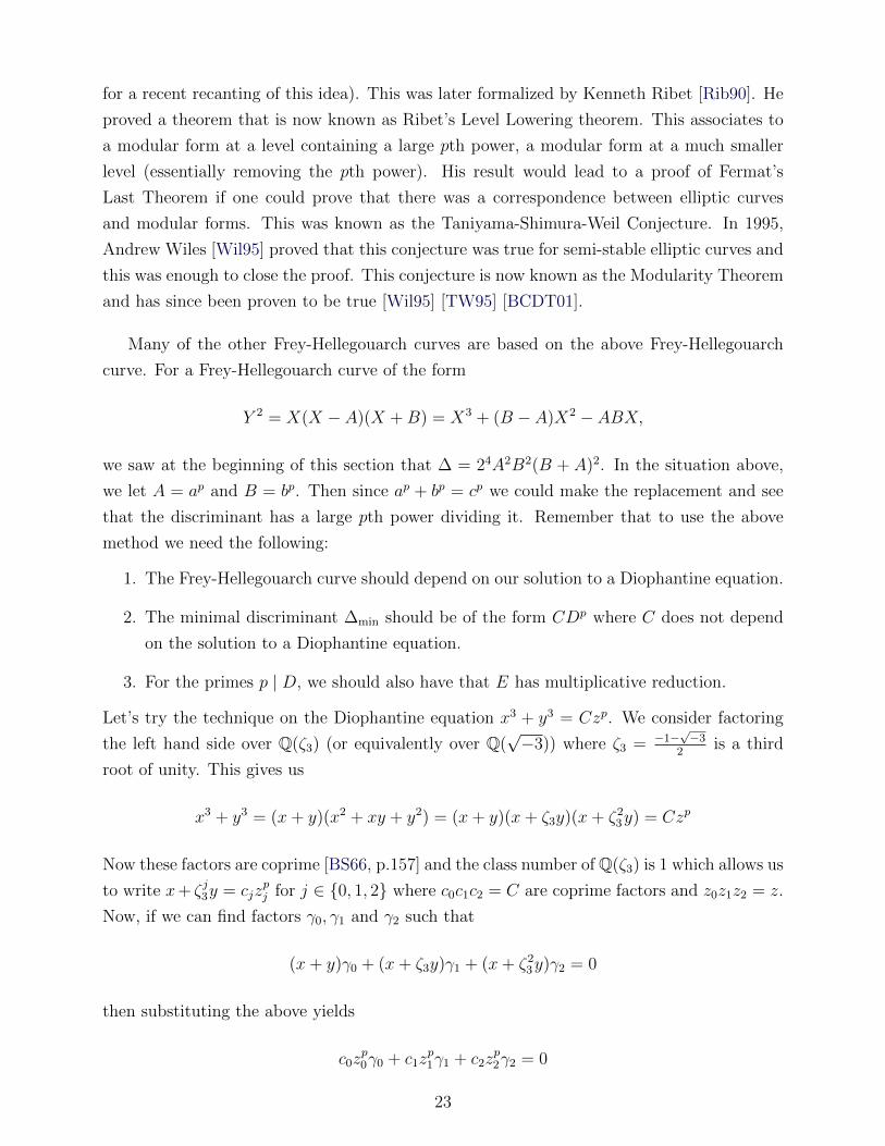
Many of the other Frey-Hellegouarch curves are based on the above Frey-Hellegouarch
curve. For a Frey-Hellegouarch curve of the form
Y 2 = X(X − A)(X +B) = X3 + (B − A)X2 − ABX,
we saw at the beginning of this section that ∆ = 24A2B2(B + A)2. In the situation above,
we let A = ap and B = bp. Then since ap + bp = cp we could make the replacement and see
that the discriminant has a large pth power dividing it. Remember that to use the above
method we need the following:
1. The Frey-Hellegouarch curve should depend on our solution to a Diophantine equation.
2. The minimal discriminant ∆min should be of the form CDp where C does not depend
on the solution to a Diophantine equation.
3. For the primes p | D, we should also have that E has multiplicative reduction.
Let’s try the technique on the Diophantine equation x3 + y3 = Czp. We consider factoring
the left hand side over Q(ζ3) (or equivalently over Q(√−3)) where ζ3 = −1−
√−3
2is a third
root of unity. This gives us
x3 + y3 = (x+ y)(x2 + xy + y2) = (x+ y)(x+ ζ3y)(x+ ζ23y) = Czp
Now these factors are coprime [BS66, p.157] and the class number of Q(ζ3) is 1 which allows us
to write x+ ζj3y = cjzpj for j ∈ 0, 1, 2 where c0c1c2 = C are coprime factors and z0z1z2 = z.
Now, if we can find factors γ0, γ1 and γ2 such that
(x+ y)γ0 + (x+ ζ3y)γ1 + (x+ ζ23y)γ2 = 0
then substituting the above yields
c0zp0γ0 + c1z
p1γ1 + c2z
p2γ2 = 0
23

and this should remind us of the original Frey-Hellegouarch curve we used above. Thus, we
search for values of γj that make the above work and then see if we get a Frey-Hellegouarch
curve. The above equation can be solved provided the following system is satisfied
γ0 + γ1 + γ2 = 0
γ0 + ζ3γ1 + ζ23γ2 = 0
Since 1 + ζ3 + ζ23 and ζ3
3 = 1, we see that γ0 = 1, γ1 = ζ3 and γ2 = ζ23 gives an admissible
solution. Inserting this information and letting
A := (x+ ζ3y)γ1 = ζ3(x+ ζ3y) B := (x+ ζ23y)γ2 = ζ2
3 (x+ ζ23y)
we have that the above Frey-Hellegouarch curve becomes
Y 2 = X3 + (B − A)X2 − ABX = X3 + ((ζ23 − ζ3)(x− y))X2 − x3 + y3
x+ yX.
Since ζ23 − ζ3 = −2ζ3 − 1 =
√−3, the above elliptic curve is not rational. However, we
can perform a quadratic twist over Q(√−3) by (−3)1/4. This is done by sending (X, Y ) 7→
(X, (−3)1/4), multiplying through by (−3)3/2 and then relabeling −3Y as Y and (−3)1/2X
as X. Performing these operations gives us the curve defined by
(−3)1/2Y 2 = X3 + (−3)1/2(x− y)X2 − x3 + y3
x+ yX
(−3)2Y 2 = (−3)3/2X3 + (−3)2(x− y)X2 − (−3)3/2x3 + y3
x+ yX
(−3Y )2 = ((−3)1/2X)3 − 3(x− y)((−3)1/2X)2 + 3x3 + y3
x+ y((−3)1/2X)
Y 2 = X3 − 3(x− y)X2 + 3
(x3 + y3
x+ y
)X
or, if we like, we can shift the above curve so that the 2-torsion point is at y − x via
X 7→ X + x− y and get the curve
Y 2 = X3 + 3xyX + x3 − y3
It is this curve used in [BLM11] and [Mul06] and we will use this curve later in this thesis. We
can perform the same computation with x5+y5 = Czp. Let’s factor the left hand side over the
totally real field Q(ζ5 + ζ−15 ) (or equivalently over Q(
√5)). Denote by α = ζ5 + ζ−1
5 = −1+√
52
(so here we choose the primitive fifth root so that this works) and α = −1−√
52
. Then factoring
24

gives
x5 + y5 = (x+ y)(x4−x3y+x2y2−xy3 + y4) = (x+ y)(x2 +αxy+ y2)(x2 + αxy+ y2) = Czp.
Similar to the above, we solve
(x+ y)2γ0 + (x2 + αxy + y2)γ1 + (x2 + αxy + y2)γ2 = 0
where the square on the linear term above aids with the algebra. A solution to the above is
given by
γ0 = 1 γ1 = α γ2 = α.
Setting
A := α(x2 + αxy + y2) B := α(x2 + αxy + y2)
and substituting into our Frey-Hellegouarch curve gives
Y 2 = X3 + (B − A)X2 − ABX = X3 + (α− α)(x2 + y2)X2 − ααx5 + y5
x+ yX.
= X3 +√
5(x2 + y2)X2 +x5 + y5
x+ yX.
As before, twisting at 51/4 yields
Y 2 = X3 + 5(x2 + y2)X2 + 5
(x5 + y5
x+ y
)X.
To extend this idea further, [Fre10, Chapter 3] has used a technique similar to the case
with signature (5, 5, p) above. He exploits the fact that Q(ζ5 + ζ−15 ) is the maximal totally
real subfield of Q(ζ5) and generalizes this idea to curves with signature (r, r, p). He then
further uses Hilbert modularity to get his correspondence between elliptic curves over a
totally real field and Hilbert modular forms as was proven by Khare and Wintenberger
[KW09a] [KW09b]. This thesis does not go into details of the methods of Hilbert modularity
however I did want to mention that this would be a source for more interesting problems in
the future.
At this time, I would like to record some more results in the same spirit as those mentioned
above here for use later.
25

1.6 Ternary Fermat-Type Diophantine Equations
Here I describe the kinds of arguments necessary to completely solve certain types of
Fermat equations. These arguments will also be used in the following chapters. Please note
that some of the notation used here involving variables is used only for the scope of this
section. To start, we will solve the Diophantine equation
Axp +Byp + zp = 0 (1.1)
where p ≥ 5 is prime and Ax,By and z are non-zero pairwise coprime integers and R :=
AB = 2a5b. We start by assuming that (x, y, z, p) is a solution to the equation defined
by 1.1. Without loss of generality, we may suppose that vq(R) < p for all primes q since
otherwise we have via the coprime condition that one of A or B is divisible by qp and so can
be brought into the corresponding xp or yp term. Without loss of generality, we may also
assume that Byp ≡ 0 (mod 2) and that Axp ≡ −1 (mod 4). We can associate to this curve
a corresponding Frey-Hellegouarch curve given by
E : Y 2 = X(X − Axp)(X +Byp)
Using Tate’s algorithm (see [Coh07b, p.542], [Sil94, p.364-368], [Pap93], [Mul06]), we see that
this curve has minimal discriminant
∆min =
24R2(xyz)2p if 16 - Byp
2−8R2(xyz)2p if 16 | Byp
and conductor N = 2αrad2(Rxyz) where α is given by
α =
1 if v2(R) = 0, 1 ≤ v2(R) ≤ 4 and y is even, or v2(R) ≥ 5
0 if v2(R) = 4 and y is odd
3 if 2 ≤ v2(R) ≤ 3 and y is odd
5 if v2(R) = 1 and y is odd.
Next we want to apply Ribet’s Theorem first verifying that our curve has no p-isogenies.
When α above equals 0 or 1, we can use Theorem 1.4.7 by noting that p ≥ 5, N is square
free and 4 divides |Etor(Q)| (since it is factored into linear terms). When α equals 3 or 5,
we can use Theorem 1.4.10 to see that E has no p-isogenies for any odd prime p. Hence, we
can apply level lowering and find a newform f ∈ Snew2 (Γ0(Np)) where Np = 2αrad2(R). As
R = 2a5b we have that rad2(R) = 1 or 5.
26

Now, if α = 0 or 1, we have that Np ∈ 1, 2, 5, 10 which is a contradiction since there
are no newforms at these levels. Thus, we may suppose that y is odd. If α = 3 and b = 0
then Np = 8 and that is also a contradiction since there are no newforms at level 8. If α = 3
but b ≥ 1 then we reduce to a curve of level Np = 40 of which there is one such isogeny class.
This gives an obstruction which the method cannot overcome. These obstructions are often
the difficulty when solving problems with this method.
The last case is when α = 5. This occurs when a = 1. If b = 0, then Np = 32 and
there is one curve at level 32. A look at the Cremona tables shows us that this curve has
complex multiplication by Z[i]. Now we use Theorem 1.4.11. Note that the j-invariant for
the Frey-Hellegouarch curve above is given by
j(E) =28(z2p − xpyp)3
(xyz)p.
To start, we may suppose that p 6= 5 or 13 since these cases were done by Denes [Den52] on
the equation xp + yp = 2zp. We proceed in cases.
Case 1: p is inert in Z[i]. This occurs when p ≡ 3 (mod 4). Recall that here x, y, z
are all odd. Notice that if q is a prime divisor of one of these three terms, then as x, y, z
are pairwise coprime, the prime q cannot divide the numerator. So the j-invariant is not an
integer. As p is not 2 and we have already considered the case p = 5, we know that p - Np
and p2 - N so this contradicts Theorem 1.4.11 unless xyz has no prime divisors. This would
mean that |xyz| = 1.
Case 2: p splits in Z[i]. This occurs when p ≡ 1 (mod 4). In this case Theorem 1.4.11
immediately tells us that N = Np and so we must have that 2αrad2(Rxyz) = 2αrad2(R).
This means that |xyz| = 1.
In either case above, we see that |xyz| = 1. Since a = 1 and b = 0, we want to find a
solution to xp + 2yp + zp = 0 with |xyz| = 1 and this can be given only by (A,B, x, y, z, p) =
(1, 2,−1, 1,−1, p). This completes the proof when b = 0.
If b ≥ 1, then we go to level Np = 160. By an exponent bound computation, we see that
B3(f) is nonzero and divisible only by the primes 2 and 3 for each of the three newforms of
level 160. As all primes outside of ` = 2 or ` = 5 satisfy Theorem 1.4.12, we see that this
means that p divides a product of twos and threes, a contradiction since p ≥ 5. This gives
us the following theorem originally proven by Kraus in generality [Kra97].
Theorem 1.6.1. (Kraus) The equation Axp + Byp + zp = 0 with AB = 2a5b and p ≥ 5 has
no nontrivial solutions with Ax,By and z are non-zero pairwise coprime integers when either
27

b = 0, a = 0, a = 1 or a ≥ 4 except for the one given by (A,B, x, y, z, p) = (1, 2,−1, 1,−1, p).
Using similar techniques, Bennett and Skinner [BS04] also proved the following
Theorem 1.6.2. (Bennett and Skinner) [BS04] Let C ∈ 1, 2, 5, 10 and n ≥ 4 be an integer.
Then the equation
xn + yn = Cz2
has no solutions in pairwise coprime integers (x, y, z) with x > y unless C = 2 and
(n, x, y, z) ∈ (5, 3,−1,±11), (4, 1,−1,±1).
Notice that this theorem also solves the cases when C = 2a, C = 5b or C = 2a5b since if
C is not squarefree, we can write C as kδm2 with δ either 0 or 1 and k = 1, 2, 5 or 10 thereby
reducing it to a case in the above theorem. Similarly, we have
Theorem 1.6.3. (Bennett and Skinner) [BS04] [Coh07b, p.507] Let p ≥ 7 be prime and
a ≥ 2 or a = 0. Then the equation
xp + 2ayp = z2
has no solutions in pairwise coprime integers (x, y, z) with |xy| > 1 and when |xy| = 1, then
the only solutions are (x, y, z) = (1, 1,±3).
Theorem 1.6.4. (Bennett and Skinner) [BS04] Let p ≥ 7 be prime and a ≥ 6 or a = 0.
Then the equation
xp + 2ayp = 5z2
has no solutions in pairwise coprime integers (x, y, z) with |xy| > 1.
Note that in the above theorem, a = 0 was a specific case of Theorem 1.6.2. Lastly, we
have
Theorem 1.6.5. (Bennett and Skinner) [BS04] Let p ≥ 7 be prime, a ≥ 6 and b ≥ 0. Then
the equation
Axp +Byp = z2
with AB = 2a5b has no nontrivial solutions with Ax,By and z are non-zero pairwise coprime
integers.
Extending the techniques above even further, we have the following results first proven
by Bennett, Vatsal, and Yasdani [BVY04].
28

Theorem 1.6.6. (Bennett, Vatsal, Yasdani) [BVY04] Let C ∈ 1, 2, 5 and p ≥ 7 a prime
and b a nonnegative integer. Then the equation
xp + yp = Cbz3
has no solutions in coprime integers x, y, z with |xy| > 1.
Theorem 1.6.7. (Bennett, Vatsal, Yasdani) [BVY04] Let p ≥ 7 a prime and b a positive
integer. Then the equation
xp + 5byp = z3
has no solutions in coprime integers x, y, z with |xy| > 1.
1.7 Results From This Thesis
After solving Fermat’s Last Theorem, what other similar types of problems can now be
solved? With the armamentarium of techniques at our disposal, there have since been a
multitude of generalizations of this method to approach many different types of Diophantine
equations, see for example any of [BS04], [BVY04], [BLM11], [Bil07], [BD10], [DG95], [Ell04],
[Kra97], [Kra98], [Sik03]. Some of these results were discussed in the previous section and
will be used later on.
In this thesis, we will look at twisted extensions of Fermat’s theorem, in particular, those
of the form xq + yq = pαzn for x, y, z, p, r, n ∈ Z with p prime, q ∈ 3, 5, α ≥ 1 and n ≥ 5
prime. Here I mention that work on the equations when α = 0 have been done by many
mathematicians, including the works of [Kra98] (17 ≤ n < 104 prime), [Bru00] (n = 4, 5),
[Dah08] (n = 5, 7, 11, 13) and [CS09] (infinitely many n, including a set of primes of Dirichlet
density 28219/44928) on the equation x3 + y3 = zn and an unpublished note by Darmon and
Kraus on the equation x5 + y5 = (2z)n for n prime. A full classification in these cases has
not currently been discovered, though not as a result of a lack of interest.
For this equation, we will discuss in Chapter 2 a classification of elliptic curves with a
nontrivial rational two torsion point and conductor with three distinct primes (with one of
them being 2). From here in Chapter 3, I will present some auxiliary results on Diophantine
equations to aid with our classification. Then we specify to two particular cases, curves
with conductor in the set S3,p = 18p, 36p, 72p and those curves with conductor in S5,p =
50p, 200p, 400p. In Chapters 4 and 5, I prove a classification on the type of primes such that
we have an elliptic curve with conductor in Sq,p and a nontrivial rational two torsion point.
We denote such primes with the notation Sq. In Chapter 6, I generalize the results from
29

[BLM11] first to the equation x5 + y5 = pαzn for the complement of the primes p classified in
Chapter 5, that is, for primes where all curves with conductor in the set S5,p do not have an
elliptic curve with a nontrivial rational two torsion point. Finally, in Chapter 7, I take both
this new result and the result from the [BLM11] paper one step further and extend the result
to a subset of the primes in Sq. In this final extension I show a specific subset of Sq,p that
the prime p must avoid in order to be in my classification. The main theorems in this thesis
are given by the following. For the purposes of stating the theorems now, I will delay the
definition of Pb,q and Pg,q until Chapter 7 but mention now that these two sets are subsets
of Sq.
Theorem 1.7.1. Suppose that p ≥ 5 and that p /∈ S5. Let α ≥ 1 be an integer. Then the
equation
x5 + y5 = pαzn
has no solutions in coprime nonzero integers x, y, z and prime n satisfying n ≥ p13p
Theorem 1.7.2. Let q ∈ 3, 5 and let p ∈ Pg,q ⊆ Sq. Then p ∈ Pb,q if and only if every
elliptic curve with conductor in Sq,p with non-trivial rational two torsion has discriminant
not of the form ∆Q,q,m :=(−1q
)qm2 for all integers m.
Theorem 1.7.3. Let q ∈ 3, 5 and suppose that p is a prime such that p 6∈ Sq or that
p ∈ Pb,q ⊆ Sq. Then the equation xq + yq = pαzn has no nontrivial coprime integer solutions
(x, y, z) where α ≥ 1 and n ≥ Cq(p) a prime. Furthermore, if the prime p avoids the lists in
Tables 7.1 and 7.3 (hence residing in Table 7.5) when q = 3 or in Tables 7.2 and 7.4 (hence
residing in Table 7.6) when q = 5, then we have that p 6∈ Sq or that p ∈ Pb,q ⊆ Sq.
30

Chapter 2
Classification of Elliptic Curves With
Nontrivial Rational Two Torsion
2.1 On the Q-Isomorphism Classes of Elliptic Curves
With Nontrivial Rational 2-Torsion and Conductor
2LqMpN
Let E be an elliptic curve over Q with rational two torsion and conductor 2LqMpN (here,
we use q first because we are interested in the case when q = 5). We know via Theorem 1.2.7
that the conductor of any such elliptic curve cannot be divisible by 29, 36, or `3 where ` ≥ 5
is a prime. Further, by [Mul06, p. 13], we know that any elliptic curve over Q with rational
two torsion is such that 33 does not divide the conductor. Thus we can assume here that
0 ≤ L ≤ 8 and 0 ≤M,N ≤ 2. We may also assume that E has a model given by
E : y2 = x3 + ax2 + bx.
For such a curve, we have that the discriminant is given by
∆ = 24b2(a2 − 4b).
From [Mul06, p.13-14], we see that the discriminant above and the conductor must share odd
primes and so we have that
b2(a2 − 4b) = ±2λqµpν
for some non-negative integers λ, µ, ν. Hence, we must have that
b = ±2iqjpk
31

for some i, j, k satisfying 0 ≤ 2i ≤ λ, 0 ≤ 2j ≤ µ and 0 ≤ 2k ≤ ν. Using this, we have that
a2 = 2i+2qjpk ± 2λ−2iqµ−2jpν−2k.
Now, break this down into 27 cases based on the trichotomies depending on if i+ 2 > λ− 2i,
i+ 2 < λ− 2i or i+ 2 = λ− 2i (and similarly with i replaced by j or k and λ replaced by µ
or ν) we can create a table of Q-isomorphism classes of curves. I will demonstrate one such
case here and for the rest I refer the interested reader to the appendix in [Mul06] though
the reader should be warned that there are numerous typos in the proof found there. Let’s
suppose that i+ 2 > λ− 2i, j = µ− 2j and k < ν − 2k. Factoring gives
a2 = 2λ−2iqjpk(23i−λ+2 ± pν−3k).
Set d := 23i−λ+2 ± pν−3k. Since a priori we do not know if q | d, we have that q(j+ε)/2 | awhere j ≡ ε (mod 2). Rewriting the above equation, we have
3ε(
a
2λ/2−iq(j+ε)/2pk/2
)2
− 23i−λ+2 = ±pν−2k
with ` := 3i − λ + 2 ≥ 1 and n := ν − 2k ≥ 1. Then depending on ε, we have a solution to
one of the following equations
d2 − 2` = ±pn or 3d2 − 2` = ±pn
if ε = 0 in the first case or ε = 1 in the second case. Either way, a model for our elliptic curve
can be given by
y2 = x3 + 2λ/2−iq(j+ε)/2pk/2dx2 + 2iqjpkx.
Now, by the division algorithm, we can write
λ/2− i = 2q1 + r1j + ε
2= 2q2 + r2 k/2 = 2q3 + r3
where r1, r2, r3 ∈ 0, 1. Rewriting the elliptic curve gives
y2 = x3 + 22q1+r1q2q2+r2p2q3+r3dx2 + 2`−2+4q1+2r1q4q2+2r2−εp4q2+2r3x.
If ` = 1 and r1 = 0, then the change of variables
(X, Y ) =
(x
22(q1−1)q2(q2+(r2−1)ε)p2q3,
y
23(q1−1)q3(q2+(r2−1)ε)p3q3
)
32

gives the Q-isomorphic curve
Y 2 = X3 + 22q2ε+(1−2ε)r2pr3dX2 + 23q3ε+2(1−2ε)r2p2r2X
If (`, r1) 6= (1, 0) (and so either ` > 1 or r1 > 0), we have that the change of variables
(X, Y ) =
(x
22q1q2(q2+(r2−1)ε)p2q3,
y
23q1q3(q2+(r2−1)ε)p3q3
)gives the Q-isomorphic curve
Y 2 = X3 + 2r1q2ε+(1−2ε)r2pr3dX2 + 2`+2r1−2q3ε+2(1−2ε)r2p2r2X.
Note that when ε = 0, the curve above corresponds to case 4 in the tables below. When
ε = 1, then the curve above corresponds to case 8 in the table below. To see this easily, plug
in for the cases of r2 ∈ 0, 1 and ε ∈ 0, 1. Modifying the above argument 26 times gives
the following theorem.
Theorem 2.1.1. (Modified from [Mul06, p. 270-271, 309-310]) Suppose E is an elliptic
curve with rational two torsion and conductor 2LqMpN . Without loss of generality, E can
take the form
E : y2 = x3 + a2x2 + a4x.
Further assume that a4 > 0. Then, there exists an integer d and non-negative integers `,m, n
satisfying one of the equations in the second column below and the corresponding curve E is
given by a2 and a4 given in the third and fourth columns where r1, r2, r3 ∈ 0, 1 except in
cases 1 through 9 (for both tables below) where if ` = 1, then r1 ∈ 1, 2 and the sign in the
Diophantine equation matches that of the sign in the discriminant ∆.
33

Equation a2 a4 ∆
1 d2 − 2`qmpn = ±1 2r1qr2pr3d 2`+2r1−2qm+2r2pn+2r3 ±22`+6r1q2m+6r2p2n+6r3
2 d2 − 2`qm = ±pn 2r1qr2pr3d 2`+2r1−2qm+2r2p2r3 ±22`+6r1q2m+6r2pn+6r3
3 d2 − 2`pn = ±qm 2r1qr2pr3d 2`+2r1−2q2r2pn+2r3 ±22`+6r1qm+6r2p2n+6r3
4 d2 − 2` = ±qmpn 2r1qr2pr3d 2`+2r1−2q2r2p2r3 ±22`+6r1qm+6r2pn+6r3
5 pd2 − 2`qm = ±1 2r1qr2pr3+1d 2`+2r1−2qm+2r2p2r3+1 ±22`+6r1q2m+6r2p6r3+3
6 pd2 − 2` = ±qm 2r1qr2pr3+1d 2`+2r1−2q2r2p2r3+1 ±22`+6r1qm+6r2p6r3+3
7 qd2 − 2`pn = ±1 2r1qr2+1pr3d 2`+2r1−2q2r2+1pn+2r3 ±22`+6r1q6r2+3p2n+6r3
8 qd2 − 2` = ±pn 2r1qr2+1pr3d 2`+2r1−2q2r2+1p2r3 ±22`+6r1q6r2+3pn+6r3
9 qpd2 − 2` = ±1 2r1qr2+1pr3+1d 2`+2r1−2q2r2+1p2r3+1 ±22`+6r1q6r2+3p6r3+3
10 d2 − qmpn = ±2` 2r1+1qr2pr3d 22r1qm+2r2pn+2r3 ±2`+6r1+6q2m+6r2p2n+6r3
11 d2 − qm = ±2`pn 2r1+1qr2pr3d 22r1qm+2r2p2r3 ±2`+6r1+6q2m+6r2pn+6r3
12 d2 − pn = ±2`qm 2r1+1qr2pr3d 22r1q2r2pn+2r3 ±2`+6r1+6qm+6r2p2n+6r3
13 d2 − 1 = ±2`qmpn 2r1+1qr2pr3d 22r1q2r2p2r3 ±2`+6r1+6qm+6r2pn+6r3
14 pd2 − qm = ±2` 2r1+1qr2pr3+1d 22r1qm+2r2p2r3+1 ±2`+6r1+6q2m+6r2p6r3+3
15 pd2 − 1 = ±2`qm 2r1+1qr2pr3+1d 22r1q2r2p2r3+1 ±2`+6r1+6qm+6r2p6r3+3
16 qd2 − pn = ±2` 2r1+1qr2+1pr3d 22r1q2r2+1pn+2r3 ±2`+6r1+6q6r2+3p2n+6r3
17 qd2 − 1 = ±2`pn 2r1+1qr2+1pr3d 22r1q2r2+1p2r3 ±2`+6r1+6q6r2+3pn+6r3
18 qpd2 − 1 = ±2` 2r1+1qr2+1pr3+1d 22r1q2r2+1p2r3+1 ±2`+6r1+6q6r2+3p6r3+3
19 2d2 − qmpn = ±1 2r1+2qr2pr3d 22r1+1qm+2r2pn+2r3 ±26r1+9q2m+6r2p2n+6r3
20 2d2 − qm = ±pn 2r1+2qr2pr3d 22r1+1qm+2r2p2r3 ±26r1+9q2m+6r2pn+6r3
21 2d2 − pn = ±qm 2r1+2qr2pr3d 22r1+1q2r2pn+2r3 ±26r1+9qm+6r2p2n+6r3
22 2d2 − 1 = ±qmpn 2r1+2qr2pr3d 22r1+1q2r2p2r3 ±26r1+9qm+6r2pn+6r3
23 2pd2 − qm = ±1 2r1+2qr2pr3+1d 22r1+1qm+2r2p2r3+1 ±26r1+9q2m+6r2p6r3+3
24 2pd2 − 1 = ±qm 2r1+2qr2pr3+1d 22r1+1q2r2p2r3+1 ±26r1+9qm+6r2p6r3+3
25 2qd2 − pn = ±1 2r1+2qr2+1pr3d 22r1+1q2r2+1pn+2r3 ±26r1+9q6r2+3p2n+6r3
26 2qd2 − 1 = ±pn 2r1+2qr2+1pr3d 22r1+1q2r2+1p2r3 ±26r1+9q6r2+3pn+6r3
27 2qpd2 − 1 = ±1 2r1+2qr2+1pr3+1d 22r1+1q2r2+1p2r3+1 ±26r1+9q6r2+3p6r3+3
Table 2.1: Elliptic curves of conductor 2LqMpN when a4 > 0
When a4 < 0, we have
34

Equation a2 a4 ∆
2 d2 + 2`qm = pn 2r1qr2pr3d −2`+2r1−2qm+2r2p2r3 22`+6r1q2m+6r2pn+6r3
3 d2 + 2lpn = qm 2r1qr2pr3d −2`+2r1−2q2r2pn+2r3 22`+6r1qm+6r2p2n+6r3
4 d2 + 2l = qmpn 2r1qr2pr3d −2`+2r1−2q2r2p2r3 22`+6r1qm+6r2pn+6r3
6 pd2 + 2l = qm 2r1qr2pr3+1d −2`+2r1−2q2r2p2r3+1 22`+6r1qm+6r2p6r3+3
8 qd2 + 2l = pn 2r1qr2+1pr3d −2`+2r1−2q2r2+1p2r3 22`+6r1q6r2+3pn+6r3
10 d2 + qmpn = 2` 2r1+1qr2pr3d −22r1qm+2r2pn+2r3 2`+6r1+6q2m+6r2p2n+6r3
11 d2 + qm = 2`pn 2r1+1qr2pr3d −22r1qm+2r2p2r3 2`+6r1+6q2m+6r2pn+6r3
12 d2 + pn = 2`qm 2r1+1qr2pr3d −22r1q2r2pn+2r3 2`+6r1+6qm+6r2p2n+6r3
13 d2 + 1 = 2`qmpn 2r1+1qr2pr3d −22r1q2r2p2r3 2`+6r1+6qm+6r2pn+6r3
14 pd2 + qm = 2` 2r1+1qr2pr3+1d −22r1qm+2r2p2r3+1 2`+6r1+6q2m+6r2p6r3+3
15 pd2 + 1 = 2`qm 2r1+1qr2pr3+1d −22r1q2r2p2r3+1 2`+6r1+6qm+6r2p6r3+3
16 qd2 + pn = 2` 2r1+1qr2+1pr3d −22r1q2r2+1pn+2r3 2`+6r1+6q6r2+3p2n+6r3
17 qd2 + 1 = 2`pn 2r1+1qr2+1pr3d −22r1q2r2+1p2r3 2`+6r1+6q6r2+3pn+6r3
18 qpd2 + 1 = 2` 2r1+1qr2+1pr3+1d −22r1q2r2+1p2r3+1 2`+6r1+6q6r2+3p6r3+3
20 2d2 + qm = pn 2r1+2qr2pr3d −22r1+1qm+2r2p2r3 26r1+9q2m+6r2pn+6r3
21 2d2 + pn = qm 2r1+2qr2pr3d −22r1+1q2r2pn+2r3 26r1+9qm+6r2p2n+6r3
22 2d2 + 1 = qmpn 2r1+2qr2pr3d −22r1+1q2r2p2r3 26r1+9qm+6r2pn+6r3
24 2pd2 + 1 = qm 2r1+2qr2pr3+1d −22r1+1q2r2p2r3+1 26r1+9qm+6r2p6r3+3
26 2qd2 + 1 = pn 2r1+2qr2+1pr3d −22r1+1q2r2+1p2r3 26r1+9q6r2+3pn+6r3
Table 2.2: Elliptic curves of conductor 2LqMpN when a4 < 0
To avoid redundancies in the lists above, in the right hand side of the equations above,
we do allow the exponent of primes on the right to be 0 and otherwise, the exponents of the
Diophantine equations are at least 1. The numbering in the second list is kept to reflect the
first list.
In our case, we are interested for application purposes in the case when q = 5. Our
goal will be to solve the above Diophantine equations in general. Then, after simplification,
ideally we would be able to remove many of the conditions on the exponents to reveal a short
and succinct list of potential elliptic curves.
2.2 Elliptic Curves With Nontrivial Rational Two Tor-
sion and Conductor 2aqbpc
In what follows, let E be an elliptic curve of conductor 2aqbpc with nontrivial rational two
torsion where p and q are distinct odd primes. By Theorem 1.2.7, we need only to consider
35

values of the exponents of the conductor where
0 ≤ a ≤ 8 0 ≤ b, c ≤ 2
The work on curves of conductor 2a3bpc has been done already and is summarized in [Mul06,
Chapter 3]. In what follows, we assume that p, q ≥ 3 are distinct primes and further that
1 ≤ b, c ≤ 2. We will create a list of all such curves below satisfying this criteria sorted by
conductor. From this list, we will focus on the curves of conductor 50p, 200p and 400p and
use tricks of Diophantine equations to simplify these results to get a succinct list of primes p
with an elliptic curve with nontrivial rational two torsion and conductor 50p, 200p or 400p.
Before we begin, we discuss some notes on the notation.
1. We are looking for curves of conductor 2aqbpc with nontrivial rational two torsion. The
idea here is to find integers `,m, n so that the curves we find fit into some appropriate
row of the tables in Section 2.1.
2. We require that m ≥ 1 when b = 1 and we can allow m = 0 when b = 2 (because then
r2 = 1), which is equivalent to asking for m ≥ 2− b for b = 1, 2.
3. The function ψ(t) returns the square root value congruent to 1 modulo 4 or the positive
value if t is even.
4. Some cases that were present in the tables above are not below. These omitted cases
are the ones with associated Diophantine equations that cannot be solved as seen by
looking at local conditions, for example by reducing modulo a power of 2 or modulo p
or q.
5. The tables below give minimal models at the primes that divide the conductor except
when 4 does not divide the conductor. In that case, one can obtain a minimal model
as stated in [Mul06, p. 13].
6. Curves denoted by E and E ′ are related by a twist by√−1.
7. Curves beginning with the same letter are linked by a degree 2 isogeny as in [Coh07a,
p. 532-533] or a composition of two such isogenies as in [Mul06, p.31].
8. The lettering used here was inspired by [Mul06]. It is unfortunate that the lettering
here does not correspond in any way to either the lettering used there or in [Cre] but
for us, the notation is self contained and so we proceed with this in mind.
Theorem 2.2.1. The elliptic curves E defined over Q of conductor qbp and having at least
one rational point of order 2 are the ones such that one of the following conditions is satisfied:
36

1. There exist integers m ≥ 2 − b and n ≥ 1 such that 26qmpn + 1 is a square and E is
Q-isomorphic to one of the following elliptic curves:
a2 a4 ∆
A1 ε · qb−1ψ(26qmpn + 1) 24qm+2(b−1)pn 212q2m+6(b−1)p2n
A2 −ε · 2 · qb−1ψ(26qmpn + 1) q2(b−1) 212qm+6(b−1)pn
where ε ∈ ±1 is the residue of qb−1 modulo 4.
2. There exist integers m ≥ 2 − b and n ≥ 1 such that 26qm + pn is a square and E is
Q-isomorphic to one of the following elliptic curves:
a2 a4 ∆
B1 ε · qb−1ψ(26qm + pn) 24qm+2(b−1) 212q2m+6(b−1)pn
B2 −ε · 2 · qb−1ψ(26qm + pn) q2(b−1)pn 212qm+6(b−1)p2n
where ε ∈ ±1 is the residue of qb−1 modulo 4.
3. There exist integers m ≥ 2−b and n ≥ 1 such that 26qm−pn is a square, p ≡ 7 (mod 8),
n odd and E is Q-isomorphic to one of the following elliptic curves:
a2 a4 ∆
C1 ε · qb−1ψ(26qm − pn) 24qm+2(b−1) −212q2m+6(b−1)pn
C2 −ε · 2 · qb−1ψ(26qm − pn) −q2(b−1)pn 212qm+6(b−1)p2n
where ε ∈ ±1 is the residue of qb−1 modulo 4.
4. There exist integers m ≥ 2 − b and n ≥ 1 such that pn − 26qm is a square and E is
Q-isomorphic to one of the following elliptic curves:
a2 a4 ∆
D1 ε · qb−1ψ(pn − 26qm) −24qm+2(b−1) 212q2m+6(b−1)pn
D2 −ε · 2 · qb−1ψ(pn − 26qm q2(b−1)pn −212qm+6(b−1)p2n
where ε ∈ ±1 is the residue of qb−1 modulo 4.
5. There exist integers m ≥ 2 − b and n ≥ 1 such that 26pn + qm is a square and E is
Q-isomorphic to one of the following elliptic curves:
a2 a4 ∆
E1 ε · qb−1ψ(26pn + qm) 24q2(b−1)pn 212qm+6(b−1)p2n
E2 −ε · 2 · qb−1ψ(26pn + qm) qm+2(b−1) 212q2m+6(b−1)pn
37

where ε ∈ ±1 is the residue of qb−1 modulo 4.
6. There exist integers m ≥ 2−b and n ≥ 1 such that 26pn−qm is a square, q ≡ 7 (mod 8),
m odd and E is Q-isomorphic to one of the following elliptic curves:
a2 a4 ∆
F1 ε · qb−1ψ(26pn − qm) 24q2(b−1)pn −212qm+6(b−1)p2n
F2 −ε · 2 · qb−1ψ(26pn − qm) −qm+2(b−1) 212q2m+6(b−1)pn
where ε ∈ ±1 is the residue of qb−1 modulo 4.
7. There exist integers m ≥ 2 − b and n ≥ 1 such that qm − 26pn is a square and E is
Q-isomorphic to one of the following elliptic curves:
a2 a4 ∆
G1 ε · qb−1ψ(qm − 26pn) −24q2(b−1)pn 212qm+6(b−1)p2n
G2 −ε · 2 · qb−1ψ(qm − 26pn) qm+2(b−1) −212q2m+6(b−1)pn
where ε ∈ ±1 is the residue of qb−1 modulo 4.
8. There exist integers m ≥ 2 − b and n ≥ 1 such that 26 + qmpn is a square and E is
Q-isomorphic to one of the following elliptic curves:
a2 a4 ∆
H1 ε · qb−1ψ(26 + qmpn) 24q2(b−1) 212qm+6(b−1)pn
H2 −ε · 2 · qb−1ψ(26 + qmpn) qm+2(b−1)pn 212q2m+6(b−1)p2n
where ε ∈ ±1 is the residue of qb−1 modulo 4.
9. There exist integers m ≥ 2 − b and n ≥ 1 such that 26 − qmpn is a square and E is
Q-isomorphic to one of the following elliptic curves:
a2 a4 ∆
I1 ε · qb−1ψ(26 − qmpn) 24q2(b−1) −212qm+6(b−1)pn
I2 −ε · 2 · qb−1ψ(26 − qmpn) −qm+2(b−1)pn 212q2m+6(b−1)p2n
where ε ∈ ±1 is the residue of qb−1 modulo 4.
10. There exist integers m ≥ 2 − b and n ≥ 1 such that qmpn − 26 is a square, 8 | (3q +
5)(q − 1), 8 | (3p + 5)(p − 1) and E is Q-isomorphic to one of the following elliptic
curves:
38
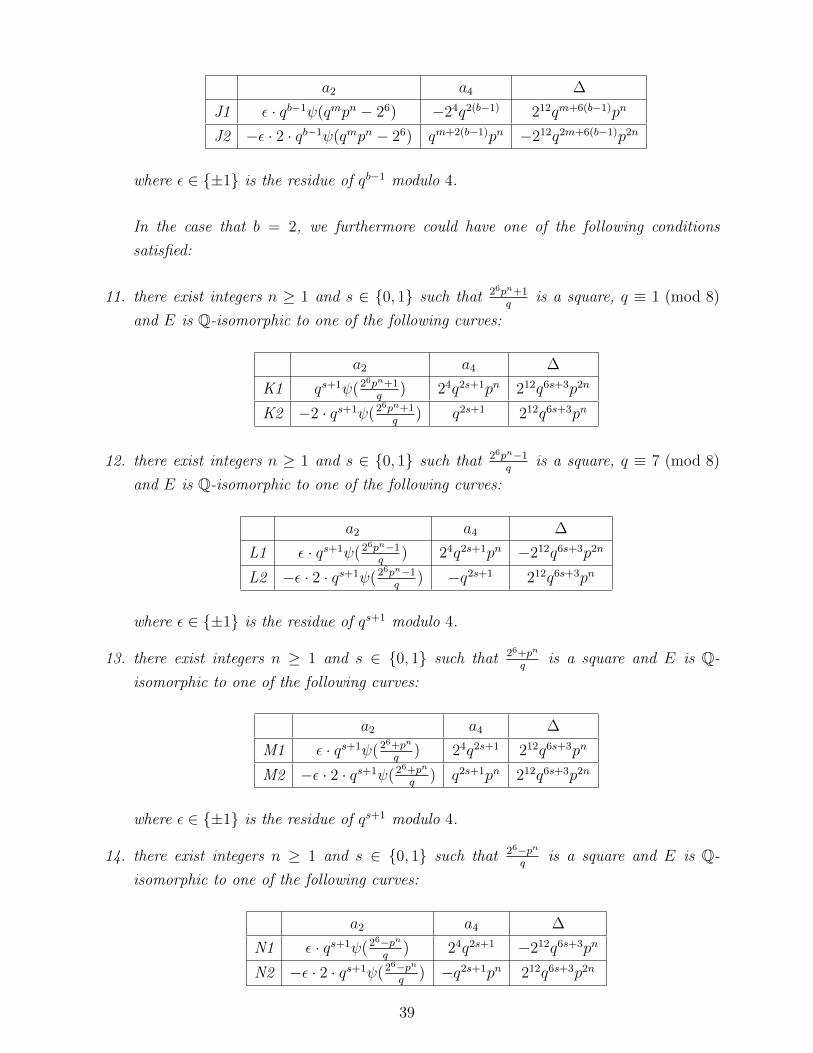
a2 a4 ∆
J1 ε · qb−1ψ(qmpn − 26) −24q2(b−1) 212qm+6(b−1)pn
J2 −ε · 2 · qb−1ψ(qmpn − 26) qm+2(b−1)pn −212q2m+6(b−1)p2n
where ε ∈ ±1 is the residue of qb−1 modulo 4.
In the case that b = 2, we furthermore could have one of the following conditions
satisfied:
11. there exist integers n ≥ 1 and s ∈ 0, 1 such that 26pn+1q
is a square, q ≡ 1 (mod 8)
and E is Q-isomorphic to one of the following curves:
a2 a4 ∆
K1 qs+1ψ(26pn+1q
) 24q2s+1pn 212q6s+3p2n
K2 −2 · qs+1ψ(26pn+1q
) q2s+1 212q6s+3pn
12. there exist integers n ≥ 1 and s ∈ 0, 1 such that 26pn−1q
is a square, q ≡ 7 (mod 8)
and E is Q-isomorphic to one of the following curves:
a2 a4 ∆
L1 ε · qs+1ψ(26pn−1q
) 24q2s+1pn −212q6s+3p2n
L2 −ε · 2 · qs+1ψ(26pn−1q
) −q2s+1 212q6s+3pn
where ε ∈ ±1 is the residue of qs+1 modulo 4.
13. there exist integers n ≥ 1 and s ∈ 0, 1 such that 26+pn
qis a square and E is Q-
isomorphic to one of the following curves:
a2 a4 ∆
M1 ε · qs+1ψ(26+pn
q) 24q2s+1 212q6s+3pn
M2 −ε · 2 · qs+1ψ(26+pn
q) q2s+1pn 212q6s+3p2n
where ε ∈ ±1 is the residue of qs+1 modulo 4.
14. there exist integers n ≥ 1 and s ∈ 0, 1 such that 26−pnq
is a square and E is Q-
isomorphic to one of the following curves:
a2 a4 ∆
N1 ε · qs+1ψ(26−pnq
) 24q2s+1 −212q6s+3pn
N2 −ε · 2 · qs+1ψ(26−pnq
) −q2s+1pn 212q6s+3p2n
39

where ε ∈ ±1 is the residue of qs+1 modulo 4.
15. there exist integers n ≥ 1 and s ∈ 0, 1 such that pn−26
qis a square and E is Q-
isomorphic to one of the following curves:
a2 a4 ∆
O1 ε · qs+1ψ(pn−26
q) −24q2s+1 212q6s+3pn
O2 −ε · 2 · qs+1ψ(pn−26
q) q2s+1pn −212q6s+3p2n
where ε ∈ ±1 is the residue of qs+1 modulo 4.
Theorem 2.2.2. The elliptic curves E defined over Q of conductor 2qbp and having at least
one rational point of order 2 are the ones such that one of the following conditions is satisfied:
1. There exist integers ` ≥ 7, m ≥ 2− b and n ≥ 1 such that 2`qmpn + 1 is a square and
E is Q-isomorphic to one of the following elliptic curves:
a2 a4 ∆
A1 ε · qb−1ψ(2`qmpn + 1) 2`−2qm+2(b−1)pn 22`q2m+6(b−1)p2n
A2 −ε · 2 · qb−1ψ(2`qmpn + 1) q2(b−1) 2`+6qm+6(b−1)pn
where ε ∈ ±1 is the residue of qb−1 modulo 4.
2. There exist integers ` ≥ 7, m ≥ 2− b and n ≥ 1 such that 2`qm + pn is a square and E
is Q-isomorphic to one of the following elliptic curves:
a2 a4 ∆
B1 ε · qb−1ψ(2`qm + pn) 2`−2qm+2(b−1) 22`q2m+6(b−1)pn
B2 −ε · 2 · qb−1ψ(2`qm + pn) q2(b−1)pn 2`+6qm+6(b−1)p2n
where ε ∈ ±1 is the residue of qb−1 modulo 4.
3. There exist integers ` ≥ 7, m ≥ 2 − b and n ≥ 1 such that 2`qm − pn is a square,
p ≡ 7 (mod 8), n odd and E is Q-isomorphic to one of the following elliptic curves:
a2 a4 ∆
C1 ε · qb−1ψ(2`qm − pn) 2`−2qm+2(b−1) −22`q2m+6(b−1)pn
C2 −ε · 2 · qb−1ψ(2`qm − pn) −q2(b−1)pn 2`+6qm+6(b−1)p2n
where ε ∈ ±1 is the residue of qb−1 modulo 4.
40

4. There exist integers ` ≥ 7, m ≥ 2− b and n ≥ 1 such that pn− 2`qm is a square and E
is Q-isomorphic to one of the following elliptic curves:
a2 a4 ∆
D1 ε · qb−1ψ(pn − 2`qm) −2`−2qm+2(b−1) 22`q2m+6(b−1)pn
D2 −ε · 2 · qb−1ψ(pn − 2`qm) q2(b−1)pn −2`+6qm+6(b−1)p2n
where ε ∈ ±1 is the residue of qb−1 modulo 4.
5. There exist integers ` ≥ 7, m ≥ 2− b and n ≥ 1 such that 2`pn + qm is a square and E
is Q-isomorphic to one of the following elliptic curves:
a2 a4 ∆
E1 ε · qb−1ψ(2`pn + qm) 2`−2q2(b−1)pn 22`qm+6(b−1)p2n
E2 −ε · 2 · qb−1ψ(2`pn + qm) qm+2(b−1) 2`+6q2m+6(b−1)pn
where ε ∈ ±1 is the residue of qb−1 modulo 4.
6. There exist integers ` ≥ 7, m ≥ 2 − b and n ≥ 1 such that 2`pn − qm is a square,
q ≡ 7 (mod 8), m odd and E is Q-isomorphic to one of the following elliptic curves:
a2 a4 ∆
F1 ε · qb−1ψ(2`pn − qm) 2`−2q2(b−1)pn −22`qm+6(b−1)p2n
F2 −ε · 2 · qb−1ψ(2`pn − qm) −qm+2(b−1) 2`+6q2m+6(b−1)pn
where ε ∈ ±1 is the residue of qb−1 modulo 4.
7. There exist integers ` ≥ 7, m ≥ 2− b and n ≥ 1 such that qm− 2`pn is a square and E
is Q-isomorphic to one of the following elliptic curves:
a2 a4 ∆
G1 ε · qb−1ψ(qm − 2`pn) −2`−2q2(b−1)pn 22`qm+6(b−1)p2n
G2 −ε · 2 · qb−1ψ(qm − 2`pn) qm+2(b−1) −2`+6q2m+6(b−1)pn
where ε ∈ ±1 is the residue of qb−1 modulo 4.
8. There exist integers ` ≥ 7, m ≥ 2− b and n ≥ 1 such that 2` + qmpn is a square and E
is Q-isomorphic to one of the following elliptic curves:
a2 a4 ∆
H1 ε · qb−1ψ(2` + qmpn) 2`−2q2(b−1) 22`qm+6(b−1)pn
H2 −ε · 2 · qb−1ψ(2` + qmpn) qm+2(b−1)pn 2`+6q2m+6(b−1)p2n
41

where ε ∈ ±1 is the residue of qb−1 modulo 4.
9. There exist integers ` ≥ 7, m ≥ 2− b and n ≥ 1 such that 2`− qmpn is a square and E
is Q-isomorphic to one of the following elliptic curves:
a2 a4 ∆
I1 ε · qb−1ψ(2` − qmpn) 2`−2q2(b−1) −22`qm+6(b−1)pn
I2 −ε · 2 · qb−1ψ(2` − qmpn) −qm+2(b−1)pn 2`+6q2m+6(b−1)p2n
where ε ∈ ±1 is the residue of qb−1 modulo 4.
10. There exist integers ` ≥ 7, m ≥ 2− b and n ≥ 1 such that qmpn− 2` is a square and E
is Q-isomorphic to one of the following elliptic curves:
a2 a4 ∆
J1 ε · qb−1ψ(qmpn − 2`) −2`−2q2(b−1) 22`qm+6(b−1)pn
J2 −ε · 2 · qb−1ψ(qmpn − 2`) qm+2(b−1)pn −2`+6q2m+6(b−1)p2n
where ε ∈ ±1 is the residue of qb−1 modulo 4.
In the case that b = 2, we furthermore could have one of the following conditions
satisfied:
11. there exist integers ` ≥ 7, n ≥ 1 and s ∈ 0, 1 such that 2`pn+1q
is a square, q ≡1 (mod 8) and E is Q-isomorphic to one of the following curves:
a2 a4 ∆
K1 qs+1ψ(2`pn+1q
) 2`−2q2s+1pn 22`q6s+3p2n
K2 −2 · qs+1ψ(2`pn+1q
) q2s+1 2`+6q6s+3pn
12. there exist integers ` ≥ 7, n ≥ 1 and s ∈ 0, 1 such that 2`pn−1q
is a square, q ≡7 (mod 8) and E is Q-isomorphic to one of the following curves:
a2 a4 ∆
L1 ε · qs+1ψ(2`pn−1q
) 2`−2q2s+1pn −22`q6s+3p2n
L2 −ε · 2 · qs+1ψ(2`pn−1q
) −q2s+1 2`+6q6s+3pn
where ε ∈ ±1 is the residue of qs+1 modulo 4.
13. there exist integers ` ≥ 7, n ≥ 1 and s ∈ 0, 1 such that 2`+pn
qis a square and E is
Q-isomorphic to one of the following curves:
42

a2 a4 ∆
M1 ε · qs+1ψ(2`+pn
q) 2`−2q2s+1 22`q6s+3pn
M2 −ε · 2 · qs+1ψ(2`+pn
q) q2s+1pn 2`+6q6s+3p2n
where ε ∈ ±1 is the residue of qs+1 modulo 4.
14. there exist integers ` ≥ 7, n ≥ 1 and s ∈ 0, 1 such that 2`−pnq
is a square and E is
Q-isomorphic to one of the following curves:
a2 a4 ∆
N1 ε · qs+1ψ(2`−pnq
) 2`−2q2s+1 −22`q6s+3pn
N2 −ε · 2 · qs+1ψ(2`−pnq
) −q2s+1pn 2`+6q6s+3p2n
where ε ∈ ±1 is the residue of qs+1 modulo 4.
15. there exist integers ` ≥ 7, n ≥ 1 and s ∈ 0, 1 such that pn−2`
qis a square and E is
Q-isomorphic to one of the following curves:
a2 a4 ∆
O1 ε · qs+1ψ(pn−2`
q) −2`−2q2s+1 22`q6s+3pn
O2 −ε · 2 · qs+1ψ(pn−2`
q) q2s+1pn −2`+6q6s+3p2n
where ε ∈ ±1 is the residue of qs+1 modulo 4.
Theorem 2.2.3. The elliptic curves E defined over Q of conductor 22qbp and having at least
one rational point of order 2 are the ones such that one of the following conditions is satisfied:
1. There exist integers m ≥ 2 − b and n ≥ 1 such that 4qm + pn is a square, qm ≡−1 (mod 4), n odd and p ≡ 5 (mod 8), and E is Q-isomorphic to one of the following
elliptic curves:
a2 a4 ∆
A1 ε · qb−1ψ(4qm + pn) qm+2(b−1) 24q2m+6(b−1)pn
A2 −ε · 2 · qb−1ψ(4qm + pn) q2(b−1)pn 28qm+6(b−1)p2n
where ε ∈ ±1 is the residue of qb−1 modulo 4.
2. There exist integers m ≥ 2 − b and n ≥ 1 such that 4qm − pn is a square, qm ≡−1 (mod 4), n odd and p ≡ 3 (mod 8), and E is Q-isomorphic to one of the following
elliptic curves:
43

a2 a4 ∆
B1 ε · qb−1ψ(4qm − pn) qm+2(b−1) −24q2m+6(b−1)pn
B2 −ε · 2 · qb−1ψ(4qm − pn) −q2(b−1)pn 28qm+6(b−1)p2n
where ε ∈ ±1 is the residue of qb−1 modulo 4.
3. There exist integers m ≥ 2−b and n ≥ 1 such that pn−4qm is a square, qm ≡ 1 (mod 4),
n odd and p ≡ 5 (mod 8), and E is Q-isomorphic to one of the following elliptic curves:
a2 a4 ∆
C1 ε · qb−1ψ(pn − 4qm) −qm+2(b−1) 24q2m+6(b−1)pn
C2 −ε · 2 · qb−1ψ(pn − 4qm) q2(b−1)pn −28qm+6(b−1)p2n
where ε ∈ ±1 is the residue of qb−1 modulo 4.
4. There exist integers m ≥ 2−b and n ≥ 1 such that 4pn+qm is a square, q ≡ 5 (mod 8),
pn ≡ −1 (mod 4) and E is Q-isomorphic to one of the following elliptic curves:
a2 a4 ∆
D1 qb−1ψ(4pn + qm) q2(b−1)pn 24qm+6(b−1)p2n
D2 −2 · qb−1ψ(4pn + qm) qm+2(b−1) 28q2m+6(b−1)pn
5. There exist integers m ≥ 2−b and n ≥ 1 such that 4pn−qm is a square, q ≡ 3 (mod 8),
pn ≡ −1 (mod 4) and E is Q-isomorphic to one of the following elliptic curves:
a2 a4 ∆
E1 ε · qb−1ψ(4pn − qm) q2(b−1)pn −24qm+6(b−1)p2n
E2 −ε · 2 · qb−1ψ(4pn − qm) −qm+2(b−1) 28q2m+6(b−1)pn
where ε ∈ ±1 is the residue of qb−1 modulo 4.
6. There exist integers m ≥ 2−b and n ≥ 1 such that qm−4pn is a square, q ≡ 5 (mod 8),
pn ≡ −1 (mod 4) and E is Q-isomorphic to one of the following elliptic curves:
a2 a4 ∆
F1 qb−1ψ(qm − 4pn) −q2(b−1)pn 24qm+6(b−1)p2n
F2 −2 · qb−1ψ(qm − 4pn) qm+2(b−1) −28q2m+6(b−1)pn
7. There exist integers m ≥ 2−b and n ≥ 1 such that qmpn−4 is a square, p, q ≡ 1 (mod 4)
and E is Q-isomorphic to one of the following elliptic curves:
44

a2 a4 ∆
G1 qb−1ψ(qmpn − 4) −q2(b−1) 24qm+6(b−1)pn
G2 −2 · qb−1ψ(qmpn − 4) qm+2(b−1)pn −210q2m+6(b−1)p2n
In the case that b = 2, we furthermore could have one of the following conditions
satisfied:
8. there exist integers n ≥ 1 and s ∈ 0, 1 such that 4pn+1q
is a square, pn ≡ 3 (mod 4),
q ≡ 5 (mod 8) and E is Q-isomorphic to one of the following curves:
a2 a4 ∆
H1 qs+1ψ(4pn+1q
) q2s+1pn 24q6s+3p2n
H2 −2 · qs+1ψ(4pn+1q
) q2s+1 28q6s+3pn
9. there exist integers n ≥ 1 and s ∈ 0, 1 such that 4pn−1q
is a square, pn ≡ 1 (mod 4),
q ≡ 3 (mod 8) and E is Q-isomorphic to one of the following curves:
a2 a4 ∆
I1 ε · qs+1ψ(4pn−1q
) q2s+1pn −24q6s+3p2n
I2 −ε · 2 · qs+1ψ(4pn−1q
) −q2s+1 28q6s+3pn
where ε ∈ ±1 is the residue of qs+1 modulo 4.
10. there exist integers n ≥ 1 and s ∈ 0, 1 such that 4+pn
qis a square, q ≡ 3 (mod 4) and
E is Q-isomorphic to one of the following curves:
a2 a4 ∆
J1 ε · qs+1ψ(4+pn
q) q2s+1 24q6s+3pn
J2 −ε · 2 · qs+1ψ(4+pn
q) q2s+1pn 28q6s+3p2n
where ε ∈ ±1 is the residue of qs+1 modulo 4.
11. there exist integers n ≥ 1 and s ∈ 0, 1 such that pn−4q
is a square, q ≡ 1 (mod 4) and
E is Q-isomorphic to one of the following curves:
a2 a4 ∆
L1 qs+1ψ(pn−4q
) −q2s+1 24q6s+3pn
L2 −2 · qs+1ψ(pn−4q
) q2s+1pn −28q6s+3p2n
45

Theorem 2.2.4. The elliptic curves E defined over Q of conductor 23qbp and having at least
one rational point of order 2 are the ones such that one of the following conditions is satisfied:
1. There exist integers ` ∈ 4, 5, m ≥ 2− b and n ≥ 1 such that 2`qmpn + 1 is a square
and E is Q-isomorphic to one of the following elliptic curves:
a2 a4 ∆
A1 ε · qb−1ψ(2`qmpn + 1) 2`−2qm+2(b−1)pn 22`q2m+6(b−1)p2n
A2 −ε · 2 · qb−1ψ(2`qmpn + 1) q2(b−1) 2`+6qm+6(b−1)pn
where ε ∈ ±1 is the residue of qb−1 modulo 4.
2. There exist integers m ≥ 2−b and n ≥ 1 such that 4qm+pn is a square, qm ≡ 1 (mod 4),
n odd and p ≡ 5 (mod 8), and E is Q-isomorphic to one of the following elliptic curves:
a2 a4 ∆
B1 −ε · qb−1ψ(4qm + pn) qm+2(b−1) 24q2m+6(b−1)pn
B2 ε · 2 · qb−1ψ(4qm + pn) q2(b−1)pn 28qm+6(b−1)p2n
where ε ∈ ±1 is the residue of qb−1 modulo 4.
3. There exist integers m ≥ 2−b and n ≥ 1 such that 4qm−pn is a square, qm ≡ 1 (mod 4),
n odd and p ≡ 3 (mod 8), and E is Q-isomorphic to one of the following elliptic curves:
a2 a4 ∆
C1 −ε · qb−1ψ(4qm − pn) qm+2(b−1) −24q2m+6(b−1)pn
C2 ε · 2 · qb−1ψ(4qm − pn) −q2(b−1)pn 28qm+6(b−1)p2n
where ε ∈ ±1 is the residue of qb−1 modulo 4.
4. There exist integers m ≥ 2 − b and n ≥ 1 such that pn − 4qm is a square, qm ≡−1 (mod 4), n odd and p ≡ 5 (mod 8), and E is Q-isomorphic to one of the following
elliptic curves:
a2 a4 ∆
D1 −ε · qb−1ψ(pn − 4qm) −qm+2(b−1) 24q2m+6(b−1)pn
D2 ε · 2 · qb−1ψ(pn − 4qm) q2(b−1)pn −28qm+6(b−1)p2n
where ε ∈ ±1 is the residue of qb−1 modulo 4.
46

5. There exist integers ` ∈ 4, 5, m ≥ 2 − b and n ≥ 1 such that 2`qm + pn is a square
and E is Q-isomorphic to one of the following elliptic curves:
a2 a4 ∆
E1 ε · qb−1ψ(2`qm + pn) 2`−2qm+2(b−1) 22`q2m+6(b−1)pn
E2 −ε · 2 · qb−1ψ(2`qm + pn) q2(b−1)pn 2`+6qm+6(b−1)p2n
where ε ∈ ±1 is the residue of qb−1 modulo 4.
6. There exist integers ` ∈ 4, 5, m ≥ 2 − b and n ≥ 1 such that 2`qm − pn is a square,
p ≡ 7 (mod 8), n odd and E is Q-isomorphic to one of the following elliptic curves:
a2 a4 ∆
F1 ε · qb−1ψ(2`qm − pn) 2`−2qm+2(b−1) −22`q2m+6(b−1)pn
F2 −ε · 2 · qb−1ψ(2`qm − pn) −q2(b−1)pn 2`+6qm+6(b−1)p2n
where ε ∈ ±1 is the residue of qb−1 modulo 4.
7. There exist integers ` ∈ 4, 5, m ≥ 2 − b and n ≥ 1 such that pn − 2`qm is a square
and E is Q-isomorphic to one of the following elliptic curves:
a2 a4 ∆
G1 ε · qb−1ψ(pn − 2`qm) −2`−2qm+2(b−1) 22`q2m+6(b−1)pn
G2 −ε · 2 · qb−1ψ(pn − 2`qm) q2(b−1)pn −2`+6qm+6(b−1)p2n
where ε ∈ ±1 is the residue of qb−1 modulo 4.
8. There exist integers m ≥ 2−b and n ≥ 1 such that 4pn+qm is a square, q ≡ 5 (mod 8),
pn ≡ 1 (mod 4) and E is Q-isomorphic to one of the following elliptic curves:
a2 a4 ∆
H1 −qb−1ψ(4pn + qm) q2(b−1)pn 24qm+6(b−1)p2n
H2 2 · qb−1ψ(4pn + qm) qm+2(b−1) 28q2m+6(b−1)pn
9. There exist integers m ≥ 2−b and n ≥ 1 such that 4pn−qm is a square, q ≡ 3 (mod 8),
pn ≡ 1 (mod 4) and E is Q-isomorphic to one of the following elliptic curves:
a2 a4 ∆
I1 −ε · qb−1ψ(4pn − qm) q2(b−1)pn −24qm+6(b−1)p2n
I2 ε · 2 · qb−1ψ(4pn − qm) −qm+2(b−1) 28q2m+6(b−1)pn
47

where ε ∈ ±1 is the residue of qb−1 modulo 4.
10. There exist integers m ≥ 2−b and n ≥ 1 such that qm−4pn is a square, q ≡ 5 (mod 8),
pn ≡ 1 (mod 4) and E is Q-isomorphic to one of the following elliptic curves:
a2 a4 ∆
J1 −qb−1ψ(qm − 4pn) −q2(b−1)pn 24qm+6(b−1)p2n
J2 2 · qb−1ψ(qm − 4pn) qm+2(b−1) −28q2m+6(b−1)pn
11. There exist integers ` ∈ 4, 5, m ≥ 2 − b and n ≥ 1 such that 2`pn + qm is a square
and E is Q-isomorphic to one of the following elliptic curves:
a2 a4 ∆
K1 ε · qb−1ψ(2`pn + qm) 2`−2q2(b−1)pn 22`qm+6(b−1)p2n
K2 −ε · 2 · qb−1ψ(2`pn + qm) qm+2(b−1) 2`+6q2m+6(b−1)pn
where ε ∈ ±1 is the residue of qb−1 modulo 4.
12. There exist integers ` ∈ 4, 5, m ≥ 2 − b and n ≥ 1 such that 2`pn − qm is a square,
q ≡ 7 (mod 8), m odd and E is Q-isomorphic to one of the following elliptic curves:
a2 a4 ∆
L1 ε · qb−1ψ(2`pn − qm) 2`−2q2(b−1)pn −22`qm+6(b−1)p2n
L2 −ε · 2 · qb−1ψ(2`pn − qm) −qm+2(b−1) 2`+6q2m+6(b−1)pn
where ε ∈ ±1 is the residue of qb−1 modulo 4.
13. There exist integers ` ∈ 4, 5, m ≥ 2 − b and n ≥ 1 such that qm − 2`pn is a square
and E is Q-isomorphic to one of the following elliptic curves:
a2 a4 ∆
M1 ε · qb−1ψ(qm − 2`pn) −2`−2q2(b−1)pn 22`qm+6(b−1)p2n
M2 −ε · 2 · qb−1ψ(qm − 2`pn) qm+2(b−1) −2`+6q2m+6(b−1)pn
where ε ∈ ±1 is the residue of qb−1 modulo 4.
14. There exist integers m ≥ 2 − b and n ≥ 1 such that 4 + qmpn is a square and E is
Q-isomorphic to one of the following elliptic curves:
a2 a4 ∆
N1 −ε · qb−1ψ(4 + qmpn) q2(b−1) 24qm+6(b−1)pn
N2 ε · 2 · qb−1ψ(4 + qmpn) qm+2(b−1)pn 28q2m+6(b−1)p2n
48

where ε ∈ ±1 is the residue of qb−1 modulo 4.
15. There exist integers ` ∈ 4, 5, m ≥ 2 − b and n ≥ 1 such that 2` + qmpn is a square
and E is Q-isomorphic to one of the following elliptic curves:
a2 a4 ∆
O1 ε · qb−1ψ(2` + qmpn) 2`−2q2(b−1) 22`qm+6(b−1)pn
O2 −ε · 2 · qb−1ψ(2` + qmpn) qm+2(b−1)pn 2`+6q2m+6(b−1)p2n
where ε ∈ ±1 is the residue of qb−1 modulo 4.
16. There exist integers ` ∈ 4, 5, m ≥ 2 − b and n ≥ 1 such that 2` − qmpn is a square
and E is Q-isomorphic to one of the following elliptic curves:
a2 a4 ∆
P1 ε · qb−1ψ(2` − qmpn) 2`−2q2(b−1) −22`qm+6(b−1)pn
P2 −ε · 2 · qb−1ψ(2` − qmpn) −qm+2(b−1)pn 2`+6q2m+6(b−1)p2n
where ε ∈ ±1 is the residue of qb−1 modulo 4.
17. There exist integers ` ∈ 4, 5, m ≥ 2 − b and n ≥ 1 such that qmpn − 2` is a square
and E is Q-isomorphic to one of the following elliptic curves:
a2 a4 ∆
Q1 ε · qb−1ψ(qmpn − 2`) −2`−2q2(b−1) 22`qm+6(b−1)pn
Q2 −ε · 2 · qb−1ψ(qmpn − 2`) qm+2(b−1)pn −2`+6q2m+6(b−1)p2n
where ε ∈ ±1 is the residue of qb−1 modulo 4.
In the case that b = 2, we furthermore could have one of the following conditions
satisfied:
18. there exist integers n ≥ 1 and s ∈ 0, 1 such that 4pn+1q
is a square, pn ≡ 1 (mod 4),
q ≡ 5 (mod 8) and E is Q-isomorphic to one of the following curves:
a2 a4 ∆
R1 −qs+1ψ(4pn+1q
) q2s+1pn 24q6s+3p2n
R2 2 · qs+1ψ(4pn+1q
) q2s+1 28q6s+3pn
19. there exist integers n ≥ 1 and s ∈ 0, 1 such that 4pn−1q
is a square, pn ≡ 3 (mod 4),
q ≡ 3 (mod 8) and E is Q-isomorphic to one of the following curves:
49
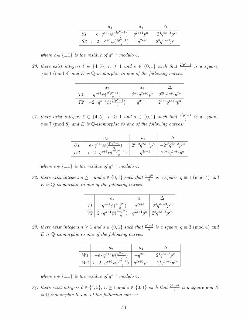
a2 a4 ∆
S1 −ε · qs+1ψ(4pn−1q
) q2s+1pn −24q6s+3p2n
S2 ε · 2 · qs+1ψ(4pn−1q
) −q2s+1 28q6s+3pn
where ε ∈ ±1 is the residue of qs+1 modulo 4.
20. there exist integers ` ∈ 4, 5, n ≥ 1 and s ∈ 0, 1 such that 2`pn+1q
is a square,
q ≡ 1 (mod 8) and E is Q-isomorphic to one of the following curves:
a2 a4 ∆
T1 qs+1ψ(2`pn+1q
) 2`−2q2s+1pn 22`q6s+3p2n
T2 −2 · qs+1ψ(2`pn+1q
) q2s+1 2`+6q6s+3pn
21. there exist integers ` ∈ 4, 5, n ≥ 1 and s ∈ 0, 1 such that 2`pn−1q
is a square,
q ≡ 7 (mod 8) and E is Q-isomorphic to one of the following curves:
a2 a4 ∆
U1 ε · qs+1ψ(2`pn−1q
) 2`−2q2s+1pn −22`q6s+3p2n
U2 −ε · 2 · qs+1ψ(2`pn−1q
) −q2s+1 2`+6q6s+3pn
where ε ∈ ±1 is the residue of qs+1 modulo 4.
22. there exist integers n ≥ 1 and s ∈ 0, 1 such that 4+pn
qis a square, q ≡ 1 (mod 4) and
E is Q-isomorphic to one of the following curves:
a2 a4 ∆
V1 −qs+1ψ(4+pn
q) q2s+1 24q6s+3pn
V2 2 · qs+1ψ(4+pn
q) q2s+1pn 28q6s+3p2n
23. there exist integers n ≥ 1 and s ∈ 0, 1 such that pn−4q
is a square, q ≡ 3 (mod 4) and
E is Q-isomorphic to one of the following curves:
a2 a4 ∆
W1 −ε · qs+1ψ(pn−4q
) −q2s+1 24q6s+3pn
W2 ε · 2 · qs+1ψ(pn−4q
) q2s+1pn −28q6s+3p2n
where ε ∈ ±1 is the residue of qs+1 modulo 4.
24. there exist integers ` ∈ 4, 5, n ≥ 1 and s ∈ 0, 1 such that 2`+pn
qis a square and E
is Q-isomorphic to one of the following curves:
50

a2 a4 ∆
X1 ε · qs+1ψ(2`+pn
q) 2`−2q2s+1 22`q6s+3pn
X2 −ε · 2 · qs+1ψ(2`+pn
q) q2s+1pn 2`+6q6s+3p2n
where ε ∈ ±1 is the residue of qs+1 modulo 4.
25. there exist integers ` ∈ 4, 5, n ≥ 1 and s ∈ 0, 1 such that 2`−pnq
is a square and E
is Q-isomorphic to one of the following curves:
a2 a4 ∆
Y1 ε · qs+1ψ(2`−pnq
) 2`−2q2s+1 −22`q6s+3pn
Y2 −ε · 2 · qs+1ψ(2`−pnq
) −q2s+1pn 2`+6q6s+3p2n
where ε ∈ ±1 is the residue of qs+1 modulo 4.
26. there exist integers ` ∈ 4, 5, n ≥ 1 and s ∈ 0, 1 such that pn−2`
qis a square and E
is Q-isomorphic to one of the following curves:
a2 a4 ∆
Z1 ε · qs+1ψ(pn−2`
q) −2`−2q2s+1 22`q6s+3pn
Z2 −ε · 2 · qs+1ψ(pn−2`
q) q2s+1pn −2`+6q6s+3p2n
where ε ∈ ±1 is the residue of qs+1 modulo 4.
Theorem 2.2.5. The elliptic curves E defined over Q of conductor 24qbp and having at least
one rational point of order 2 are the ones such that one of the following conditions is satisfied:
1. There exist integers ` ≥ 4, m ≥ 2− b and n ≥ 1 such that 2lqmpn + 1 is a square and
E is Q-isomorphic to one of the following elliptic curves:
a2 a4 ∆
A1 −ε · qb−1ψ(2lqmpn + 1) 2l−2qm+2(b−1)pn 22lq2m+6(b−1)p2n
A2 ε · 2 · qb−1ψ(2lqmpn + 1) q2(b−1) 2l+6qm+6(b−1)pn
where ε ∈ ±1 is the residue of qb−1 modulo 4.
2. There exist integers m ≥ 2−b and n ≥ 1 such that 4qm+pn is a square, qm ≡ 1 (mod 4),
n even or p ≡ 1 (mod 4), and E is Q-isomorphic to one of the following elliptic curves:
a2 a4 ∆
B1 ε · qb−1ψ(4qm + pn) qm+2(b−1) 24q2m+6(b−1)pn
B2 −ε · 2 · qb−1ψ(4qm + pn) q2(b−1)pn 28qm+6(b−1)p2n
51

where ε ∈ ±1 is the residue of qm+b−1 modulo 4.
3. There exist integers m ≥ 2−b and n ≥ 1 such that 4qm−pn is a square, qm ≡ 1 (mod 4),
n odd and p ≡ 3 (mod 8), and E is Q-isomorphic to one of the following elliptic curves:
a2 a4 ∆
C1 ε · qb−1ψ(4qm − pn) qm+2(b−1) −24q2m+6(b−1)pn
C2 −ε · 2 · qb−1ψ(4qm − pn) −q2(b−1)pn 28qm+6(b−1)p2n
where ε ∈ ±1 is the residue of qm+b−1 modulo 4.
4. There exist integers m ≥ 2 − b and n ≥ 1 such that pn − 4qm is a square, qm ≡−1 (mod 4), n even or p ≡ 1 (mod 4), and E is Q-isomorphic to one of the following
elliptic curves:
a2 a4 ∆
D1 ε · qb−1ψ(pn − 4qm) −qm+2(b−1) 24q2m+6(b−1)pn
D2 −ε · 2 · qb−1ψ(pn − 4qm) q2(b−1)pn −28qm+6(b−1)p2n
where ε ∈ ±1 is the residue of qm+b−1 modulo 4.
5. There exist integers ` ≥ 4, m ≥ 2− b and n ≥ 1 such that 2lqm + pn is a square and E
is Q-isomorphic to one of the following elliptic curves:
a2 a4 ∆
E1 −ε · qb−1ψ(2lqm + pn) 2l−2qm+2(b−1) 22lq2m+6(b−1)pn
E2 ε · 2 · qb−1ψ(2lqm + pn) q2(b−1)pn 2l+6qm+6(b−1)p2n
where ε ∈ ±1 is the residue of qb−1 modulo 4.
6. There exist integers ` ≥ 4, m ≥ 2 − b and n ≥ 1 such that 2lqm − pn is a square,
p ≡ 7 (mod 8), n odd and E is Q-isomorphic to one of the following elliptic curves:
a2 a4 ∆
F1 −ε · qb−1ψ(2lqm − pn) 2l−2qm+2(b−1) −22lq2m+6(b−1)pn
F2 ε · 2 · qb−1ψ(2lqm − pn) −q2(b−1)pn 2l+6qm+6(b−1)p2n
where ε ∈ ±1 is the residue of qb−1 modulo 4.
7. There exist integers ` ≥ 4, m ≥ 2− b and n ≥ 1 such that pn− 2lqm is a square and E
is Q-isomorphic to one of the following elliptic curves:
52

a2 a4 ∆
G1 −ε · qb−1ψ(pn − 2lqm) −2l−2qm+2(b−1) 22lq2m+6(b−1)pn
G2 ε · 2 · qb−1ψ(pn − 2lqm) q2(b−1)pn −2l+6qm+6(b−1)p2n
where ε ∈ ±1 is the residue of qb−1 modulo 4.
8. There exist integers m ≥ 2−b and n ≥ 1 such that 4pn+qm is a square, q ≡ 5 (mod 8),
pn ≡ 1 (mod 4) and E is Q-isomorphic to one of the following elliptic curves:
a2 a4 ∆
H1 qb−1ψ(4pn + qm) q2(b−1)pn 24qm+6(b−1)p2n
H2 −2 · qb−1ψ(4pn + qm) qm+2(b−1) 28q2m+6(b−1)pn
9. There exist integers m ≥ 2− b and n ≥ 1 such that 4pn−qm is a square, q ≡ 3 (mod 8)
and E is Q-isomorphic to one of the following elliptic curves:
a2 a4 ∆
I1 ε · qb−1ψ(4pn − qm) q2(b−1)pn −24qm+6(b−1)p2n
I2 −ε · 2 · qb−1ψ(4pn − qm) −qm+2(b−1) 28q2m+6(b−1)pn
where ε ∈ ±1 is the residue of qb−1pn modulo 4.
10. There exist integers m ≥ 2−b and n ≥ 1 such that qm−4pn is a square, q ≡ 5 (mod 8),
pn ≡ −1 (mod 4) and E is Q-isomorphic to one of the following elliptic curves:
a2 a4 ∆
J1 qb−1ψ(qm − 4pn) −q2(b−1)pn 24qm+6(b−1)p2n
J2 −2 · qb−1ψ(qm − 4pn) qm+2(b−1) −28q2m+6(b−1)pn
11. There exist integers ` ≥ 4, m ≥ 2− b and n ≥ 1 such that 2lpn + qm is a square and E
is Q-isomorphic to one of the following elliptic curves:
a2 a4 ∆
K1 −ε · qb−1ψ(2lpn + qm) 2l−2q2(b−1)pn 22lqm+6(b−1)p2n
K2 ε · 2 · qb−1ψ(2lpn + qm) qm+2(b−1) 2l+6q2m+6(b−1)pn
where ε ∈ ±1 is the residue of qb−1 modulo 4.
12. There exist integers ` ≥ 4, m ≥ 2 − b and n ≥ 1 such that 2lpn − qm is a square,
q ≡ 7 (mod 8), m odd and E is Q-isomorphic to one of the following elliptic curves:
53

a2 a4 ∆
L1 −ε · qb−1ψ(2lpn − qm) 2l−2q2(b−1)pn −22lqm+6(b−1)p2n
L2 ε · 2 · qb−1ψ(2lpn − qm) −qm+2(b−1) 2l+6q2m+6(b−1)pn
where ε ∈ ±1 is the residue of qb−1 modulo 4.
13. There exist integers ` ≥ 4, m ≥ 2− b and n ≥ 1 such that qm− 2lpn is a square and E
is Q-isomorphic to one of the following elliptic curves:
a2 a4 ∆
M1 −ε · qb−1ψ(qm − 2lpn) −2l−2q2(b−1)pn 22lqm+6(b−1)p2n
M2 ε · 2 · qb−1ψ(qm − 2lpn) qm+2(b−1) −2l+6q2m+6(b−1)pn
where ε ∈ ±1 is the residue of qb−1 modulo 4.
14. There exist integers m ≥ 2 − b and n ≥ 1 such that 4 + qmpn is a square and E is
Q-isomorphic to one of the following elliptic curves:
a2 a4 ∆
N1 ε · qb−1ψ(4 + qmpn) q2(b−1) 24qm+6(b−1)pn
N2 −ε · 2 · qb−1ψ(4 + qmpn) qm+2(b−1)pn 28q2m+6(b−1)p2n
where ε ∈ ±1 is the residue of qb−1 modulo 4.
15. There exist integers m ≥ 2−b and n ≥ 1 such that qmpn−4 is a square, p ≡ 1 (mod 4),
q ≡ 1 (mod 4) if m ≥ 1 and E is Q-isomorphic to one of the following elliptic curves:
a2 a4 ∆
O1 −ε · qb−1ψ(qmpn − 4) −q2(b−1) 24qm+6(b−1)pn
O2 ε · 2 · qb−1ψ(qmpn − 4) qm+2(b−1)pn −210q2m+6(b−1)p2n
where ε ∈ ±1 is the residue of qb−1 modulo 4.
16. There exist integers ` ≥ 4, m ≥ 2− b and n ≥ 1 such that 2l + qmpn is a square and E
is Q-isomorphic to one of the following elliptic curves:
a2 a4 ∆
P1 −ε · qb−1ψ(2l + qmpn) 2l−2q2(b−1) 22lqm+6(b−1)pn
P2 ε · 2 · qb−1ψ(2l + qmpn) qm+2(b−1)pn 2l+6q2m+6(b−1)p2n
where ε ∈ ±1 is the residue of qb−1 modulo 4.
54

17. There exist integers ` ≥ 4, m ≥ 2− b and n ≥ 1 such that 2l − qmpn is a square and E
is Q-isomorphic to one of the following elliptic curves:
a2 a4 ∆
Q1 −ε · qb−1ψ(2l − qmpn) 2l−2q2(b−1) −22lqm+6(b−1)pn
Q2 ε · 2 · qb−1ψ(2l − qmpn) −qm+2(b−1)pn 2l+6q2m+6(b−1)p2n
where ε ∈ ±1 is the residue of qb−1 modulo 4.
18. There exist integers ` ≥ 4, m ≥ 2− b and n ≥ 1 such that qlpn− 2m is a square and E
is Q-isomorphic to one of the following elliptic curves:
a2 a4 ∆
R1 −ε · qb−1ψ(qlpn − 2m) −2l−2q2(b−1) 22lqm+6(b−1)pn
R2 ε · 2 · qb−1ψ(qlpn − 2m) qm+2(b−1)pn −2l+6q2m+6(b−1)p2n
where ε ∈ ±1 is the residue of qb−1 modulo 4.
In the case that b = 2, we furthermore could have one of the following conditions
satisfied:
19. there exist integers n ≥ 1 and s ∈ 0, 1 such that 4pn+1q
is a square, pn ≡ 1 (mod 4),
q ≡ 5 (mod 8) and E is Q-isomorphic to one of the following curves:
a2 a4 ∆
S1 qs+1ψ(4pn+1q
) q2s+1pn 24q6s+3p2n
S2 −2 · qs+1ψ(4pn+1q
) q2s+1 28q6s+3pn
20. there exist integers n ≥ 1 and s ∈ 0, 1 such that 4pn−1q
is a square, pn ≡ 3 (mod 4),
q ≡ 3 (mod 8) and E is Q-isomorphic to one of the following curves:
a2 a4 ∆
T1 ε · qs+1ψ(4pn−1q
) q2s+1pn −24q6s+3p2n
T2 −ε · 2 · qs+1ψ(4pn−1q
) −q2s+1 28q6s+3pn
where ε ∈ ±1 is the residue of qspn modulo 4.
21. there exist integers ` ≥ 4, n ≥ 1 and s ∈ 0, 1 such that 2lpn+1q
is a square, q ≡1 (mod 8) and E is Q-isomorphic to one of the following curves:
55

a2 a4 ∆
U1 −qs+1ψ(2lpn+1q
) 2l−2q2s+1pn 22lq6s+3p2n
U2 2 · qs+1ψ(2lpn+1q
) q2s+1 2l+6q6s+3pn
22. there exist integers ` ≥ 4, n ≥ 1 and s ∈ 0, 1 such that 2lpn−1q
is a square, q ≡7 (mod 8) and E is Q-isomorphic to one of the following curves:
a2 a4 ∆
V1 −ε · qs+1ψ(2lpn−1q
) 2l−2q2s+1pn −22lq6s+3p2n
V2 ε · 2 · qs+1ψ(2lpn−1q
) −q2s+1 2l+6q6s+3pn
where ε ∈ ±1 is the residue of qs+1 modulo 4.
23. there exist integers n ≥ 1 and s ∈ 0, 1 such that 4+pn
qis a square and E is Q-
isomorphic to one of the following curves:
a2 a4 ∆
W1 εqs+1ψ(4+pn
q) q2s+1 24q6s+3pn
W2 −ε2 · qs+1ψ(4+pn
q) q2s+1pn 28q6s+3p2n
where ε ∈ ±1 is the residue of qs modulo 4.
24. there exist integers n ≥ 1 and s ∈ 0, 1 such that pn−4q
is a square and E is Q-
isomorphic to one of the following curves:
a2 a4 ∆
X1 ε · qs+1ψ(pn−4q
) −q2s+1 24q6s+3pn
X2 −ε · 2 · qs+1ψ(pn−4q
) q2s+1pn −28q6s+3p2n
where ε ∈ ±1 is the residue of −qs modulo 4.
25. there exist integers ` ≥ 4, n ≥ 1 and s ∈ 0, 1 such that 2l+pn
qis a square and E is
Q-isomorphic to one of the following curves:
a2 a4 ∆
Y1 −ε · qs+1ψ(2l+pn
q) 2l−2q2s+1 22lq6s+3pn
Y2 ε · 2 · qs+1ψ(2l+pn
q) q2s+1pn 2l+6q6s+3p2n
where ε ∈ ±1 is the residue of qs+1 modulo 4.
56
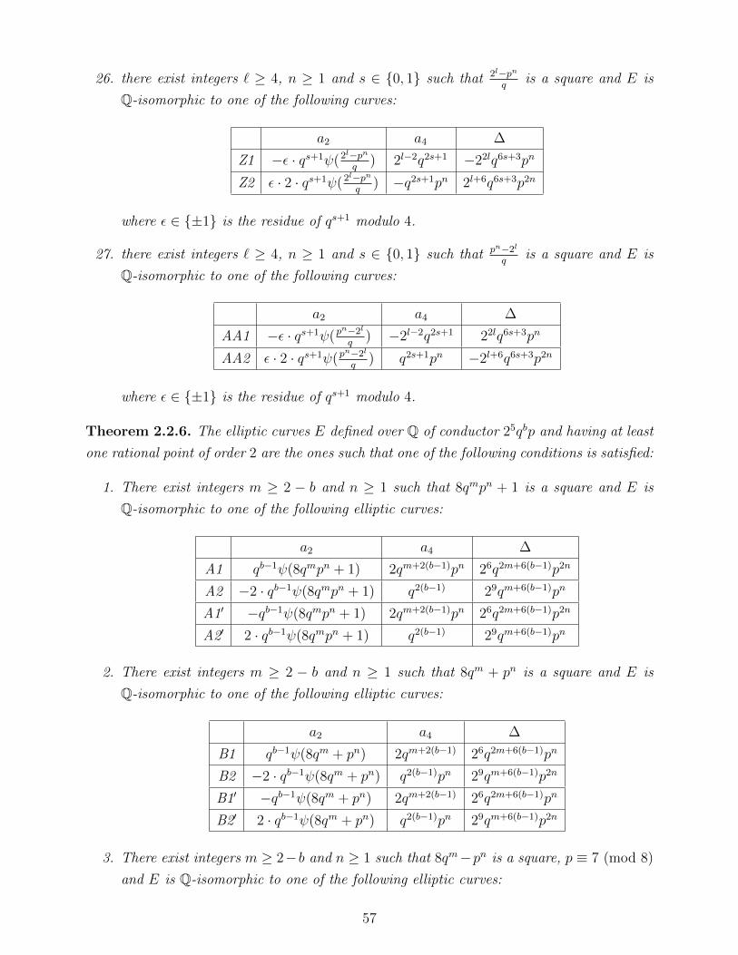
26. there exist integers ` ≥ 4, n ≥ 1 and s ∈ 0, 1 such that 2l−pnq
is a square and E is
Q-isomorphic to one of the following curves:
a2 a4 ∆
Z1 −ε · qs+1ψ(2l−pnq
) 2l−2q2s+1 −22lq6s+3pn
Z2 ε · 2 · qs+1ψ(2l−pnq
) −q2s+1pn 2l+6q6s+3p2n
where ε ∈ ±1 is the residue of qs+1 modulo 4.
27. there exist integers ` ≥ 4, n ≥ 1 and s ∈ 0, 1 such that pn−2l
qis a square and E is
Q-isomorphic to one of the following curves:
a2 a4 ∆
AA1 −ε · qs+1ψ(pn−2l
q) −2l−2q2s+1 22lq6s+3pn
AA2 ε · 2 · qs+1ψ(pn−2l
q) q2s+1pn −2l+6q6s+3p2n
where ε ∈ ±1 is the residue of qs+1 modulo 4.
Theorem 2.2.6. The elliptic curves E defined over Q of conductor 25qbp and having at least
one rational point of order 2 are the ones such that one of the following conditions is satisfied:
1. There exist integers m ≥ 2 − b and n ≥ 1 such that 8qmpn + 1 is a square and E is
Q-isomorphic to one of the following elliptic curves:
a2 a4 ∆
A1 qb−1ψ(8qmpn + 1) 2qm+2(b−1)pn 26q2m+6(b−1)p2n
A2 −2 · qb−1ψ(8qmpn + 1) q2(b−1) 29qm+6(b−1)pn
A1′ −qb−1ψ(8qmpn + 1) 2qm+2(b−1)pn 26q2m+6(b−1)p2n
A2′ 2 · qb−1ψ(8qmpn + 1) q2(b−1) 29qm+6(b−1)pn
2. There exist integers m ≥ 2 − b and n ≥ 1 such that 8qm + pn is a square and E is
Q-isomorphic to one of the following elliptic curves:
a2 a4 ∆
B1 qb−1ψ(8qm + pn) 2qm+2(b−1) 26q2m+6(b−1)pn
B2 −2 · qb−1ψ(8qm + pn) q2(b−1)pn 29qm+6(b−1)p2n
B1′ −qb−1ψ(8qm + pn) 2qm+2(b−1) 26q2m+6(b−1)pn
B2′ 2 · qb−1ψ(8qm + pn) q2(b−1)pn 29qm+6(b−1)p2n
3. There exist integers m ≥ 2− b and n ≥ 1 such that 8qm−pn is a square, p ≡ 7 (mod 8)
and E is Q-isomorphic to one of the following elliptic curves:
57

a2 a4 ∆
C1 qb−1ψ(8qm − pn) 2qm+2(b−1) −26q2m+6(b−1)pn
C2 −2 · qb−1ψ(8qm − pn) −q2(b−1)pn 29qm+6(b−1)p2n
C1′ −qb−1ψ(8qm − pn) 2qm+2(b−1) −26q2m+6(b−1)pn
C2′ 2 · qb−1ψ(8qm − pn) −q2(b−1)pn 29qm+6(b−1)p2n
4. There exist integers m ≥ 2 − b and n ≥ 1 such that pn − 8qm is a square and E is
Q-isomorphic to one of the following elliptic curves:
a2 a4 ∆
D1 qb−1ψ(pn − 8qm −2qm+2(b−1) 26q2m+6(b−1)pn
D2 −2 · qb−1ψ(pn − 8qm q2(b−1)pn −29qm+6(b−1)p2n
D1′ −qb−1ψ(pn − 8qm −2qm+2(b−1) 26q2m+6(b−1)pn
D2′ 2 · qb−1ψ(pn − 8qm q2(b−1)pn −29qm+6(b−1)p2n
5. There exist integers m ≥ 2 − b and n ≥ 1 such that 8pn + qm is a square and E is
Q-isomorphic to one of the following elliptic curves:
a2 a4 ∆
E1 qb−1ψ(8pn + qm) 2q2(b−1)pn 26qm+6(b−1)p2n
E2 −2 · qb−1ψ(8pn + qm) qm+2(b−1) 29q2m+6(b−1)pn
E1′ −qb−1ψ(8pn + qm) 2q2(b−1)pn 26qm+6(b−1)p2n
E2′ 2 · qb−1ψ(8pn + qm) qm+2(b−1) 29q2m+6(b−1)pn
6. There exist integers m ≥ 2−b and n ≥ 1 such that 8pn−qm is a square, q ≡ 7 (mod 8),
m odd and E is Q-isomorphic to one of the following elliptic curves:
a2 a4 ∆
F1 qb−1ψ(8pn − qm) 2q2(b−1)pn −26qm+6(b−1)p2n
F2 −2 · qb−1ψ(8pn − qm) −qm+2(b−1) 29q2m+6(b−1)pn
F1′ −qb−1ψ(8pn − qm) 2q2(b−1)pn −26qm+6(b−1)p2n
F2′ 2 · qb−1ψ(8pn − qm) −qm+2(b−1) 29q2m+6(b−1)pn
7. There exist integers m ≥ 2 − b and n ≥ 1 such that qm − 8pn is a square and E is
Q-isomorphic to one of the following elliptic curves:
a2 a4 ∆
G1 qb−1ψ(qm − 8pn) −2q2(b−1)pn 26qm+6(b−1)p2n
G2 −2 · qb−1ψ(qm − 8pn) qm+2(b−1) −29q2m+6(b−1)pn
G1′ −qb−1ψ(qm − 8pn) −2q2(b−1)pn 26qm+6(b−1)p2n
G2′ 2 · qb−1ψ(qm − 8pn) qm+2(b−1) −29q2m+6(b−1)pn
58

8. There exist integers m ≥ 2 − b and n ≥ 1 such that 8 + qmpn is a square, p ≡1, 7 (mod 8), q ≡ 1, 7 (mod 8) if m > 0, and E is Q-isomorphic to one of the following
elliptic curves:
a2 a4 ∆
H1 qb−1ψ(8 + qmpn) 2q2(b−1) 26qm+6(b−1)pn
H2 −2 · qb−1ψ(8 + qmpn) qm+2(b−1)pn 29q2m+6(b−1)p2n
H1′ −qb−1ψ(8 + qmpn) 2q2(b−1) 26qm+6(b−1)pn
H2′ 2 · qb−1ψ(8 + qmpn) qm+2(b−1)pn 29q2m+6(b−1)p2n
9. There exist integers m ≥ 2 − b and n ≥ 1 such that qmpn − 8 is a square, p ≡1, 3 (mod 8), q ≡ 1, 3 (mod 8) if m > 0, and E is Q-isomorphic to one of the following
elliptic curves:
a2 a4 ∆
I1 qb−1ψ(qmpn − 8) −2q2(b−1) 26qm+6(b−1)pn
I2 −2 · qb−1ψ(qmpn − 8) qm+2(b−1)pn −29q2m+6(b−1)p2n
I1′ −qb−1ψ(qmpn − 8) −2q2(b−1) 26qm+6(b−1)pn
I2′ 2 · qb−1ψ(qmpn − 8) qm+2(b−1)pn −29q2m+6(b−1)p2n
10. There exist integers m ≥ 2 − b and n ≥ 1 such that qmpn + 1 is a square and E is
Q-isomorphic to one of the following elliptic curves:
a2 a4 ∆
J1 2qb−1ψ(qmpn + 1) qm+2(b−1)pn 26q2m+6(b−1)p2n
J2 −4 · qb−1ψ(qmpn + 1) 4q2(b−1) 212qm+6(b−1)pn
J1′ −2qb−1ψ(qmpn + 1) qm+2(b−1)pn 26q2m+6(b−1)p2n
J2′ 4 · qb−1ψ(qmpn + 1) 4q2(b−1) 212qm+6(b−1)pn
11. There exist integers m ≥ 2− b and n ≥ 1 such that qmpn−1 is a square, p ≡ 1 (mod 4)
if n > 0, q ≡ 1 (mod 4) if m > 0, and E is Q-isomorphic to one of the following elliptic
curves:
a2 a4 ∆
K1 2qb−1ψ(qmpn − 1) q2(b−1) 26q2m+6(b−1)p2n
K2 −4 · qb−1ψ(qmpn − 1) 4qm+2(b−1)pn 212qm+6(b−1)pn
K1′ −2qb−1ψ(qmpn − 1) q2(b−1) 26q2m+6(b−1)p2n
K2′ 4 · qb−1ψ(qmpn − 1) 4qm+2(b−1)pn 212qm+6(b−1)pn
59

12. There exist integers m ≥ 2 − b and n ≥ 1 such that qm + pn is a square and E is
Q-isomorphic to one of the following elliptic curves:
(a) m is even or q ≡ 1 (mod 4);
a2 a4 ∆
L1 2qb−1ψ(qm + pn) q2(b−1)pn 26qm+6(b−1)p2n
L2 −4 · qb−1ψ(qm + pn) 4qm+2(b−1) 212q2m+6(b−1)pn
L1′ −2qb−1ψ(qm + pn) q2(b−1)pn 26qm+6(b−1)p2n
L2′ 4 · qb−1ψ(qm + pn) 4qm+2(b−1) 212q2m+6(b−1)pn
(b) m is odd and q ≡ 3 (mod 4);
a2 a4 ∆
M1 2qb−1ψ(qm + pn) qm+2(b−1) 26q2m+6(b−1)pn
M2 −4 · qb−1ψ(qm + pn) 4q2(b−1)pn 212qm+6(b−1)p2n
M1′ −2qb−1ψ(qm + pn) qm+2(b−1) 26q2m+6(b−1)pn
M2′ 4 · qb−1ψ(qm + pn) 4q2(b−1)pn 212qm+6(b−1)p2n
13. There exist integers m ≥ 2 − b and n ≥ 1 such that qm − pn is a square and E is
Q-isomorphic to one of the following elliptic curves:
(a) m is even or q ≡ 1 (mod 4);
a2 a4 ∆
N1 2qb−1ψ(qm − pn) −q2(b−1)pn 26qm+6(b−1)p2n
N2 −4 · qb−1ψ(qm − pn) 4qm+2(b−1) −212q2m+6(b−1)pn
N1′ −2qb−1ψ(qm − pn) −q2(b−1)pn 26qm+6(b−1)p2n
N2′ 4 · qb−1ψ(qm − pn) 4qm+2(b−1) −212q2m+6(b−1)pn
(b) m is odd and q ≡ 3 (mod 4);
a2 a4 ∆
O1 2qb−1ψ(qm − pn) qm+2(b−1) −26q2m+6(b−1)pn
O2 −4 · qb−1ψ(qm − pn) −4q2(b−1)pn 212qm+6(b−1)p2n
O1′ −2qb−1ψ(qm − pn) qm+2(b−1) −26q2m+6(b−1)pn
O2′ 4 · qb−1ψ(qm − pn) −4q2(b−1)pn 212qm+6(b−1)p2n
14. There exist integers m ≥ 2 − b and n ≥ 1 such that pn − qm is a square and E is
Q-isomorphic to one of the following elliptic curves:
(a) m is even or q ≡ 1 (mod 4);
60

a2 a4 ∆
P1 2qb−1ψ(pn − qm) −q2(b−1)pn 26qm+6(b−1)p2n
P2 −4 · qb−1ψ(pn − qm) 4qm+2(b−1) −212q2m+6(b−1)pn
P1′ −2qb−1ψ(pn − qm) −q2(b−1)pn 26qm+6(b−1)p2n
P2′ 4 · qb−1ψ(pn − qm) 4qm+2(b−1) −212q2m+6(b−1)pn
(b) m is odd and q ≡ 3 (mod 4);
a2 a4 ∆
Q1 2qb−1ψ(pn − qm) qm+2(b−1) −26q2m+6(b−1)pn
Q2 −4 · qb−1ψ(pn − qm) −4q2(b−1)pn 212qm+6(b−1)p2n
Q1′ −2qb−1ψ(pn − qm) qm+2(b−1) −26q2m+6(b−1)pn
Q2′ 4 · qb−1ψ(pn − qm) −4q2(b−1)pn 212qm+6(b−1)p2n
In the case that b = 2, we furthermore could have one of the following conditions
satisfied:
15. there exist integers n ≥ 1 and s ∈ 0, 1 such that 8pn+1q
is a square, q ≡ 1 (mod 8)
and E is Q-isomorphic to one of the following curves:
a2 a4 ∆
R1 qs+1ψ(8pn+1q
) 2q2s+1pn 26q6s+3p2n
R2 −2 · qs+1ψ(8pn+1q
) q2s+1 29q6s+3pn
R1′ −qs+1ψ(8pn+1q
) 2q2s+1pn 26q6s+3p2n
R2′ 2 · qs+1ψ(8pn+1q
) q2s+1 29q6s+3pn
16. there exist integers n ≥ 1 and s ∈ 0, 1 such that 8pn−1q
is a square, q ≡ 7 (mod 8)
and E is Q-isomorphic to one of the following curves:
a2 a4 ∆
S1 qs+1ψ(8pn−1q
) 2q2s+1pn −26q6s+3p2n
S2 −2 · qs+1ψ(8pn−1q
) −q2s+1 29q6s+3pn
S1′ −qs+1ψ(8pn−1q
) 2q2s+1pn −26q6s+3p2n
S2′ 2 · qs+1ψ(8pn−1q
) −q2s+1 29q6s+3pn
17. there exist integers n ≥ 1 and s ∈ 0, 1 such that 8+pn
qis a square and E is Q-
isomorphic to one of the following curves:
61

a2 a4 ∆
T1 qs+1ψ(8+pn
q) 2q2s+1 26q6s+3pn
T2 −2 · qs+1ψ(8+pn
q) q2s+1pn 29q6s+3p2n
T1′ −qs+1ψ(8+pn
q) 2q2s+1 26q6s+3pn
T2′ 2 · qs+1ψ(8+pn
q) q2s+1pn 29q6s+3p2n
18. there exist integers n ≥ 1 and s ∈ 0, 1 such that 8−pnq
is a square and E is Q-
isomorphic to one of the following curves:
a2 a4 ∆
U1 qs+1ψ(8−pnq
) 2q2s+1 −26q6s+3pn
U2 −2 · qs+1ψ(8−pnq
) −q2s+1pn 29q6s+3p2n
U1′ −qs+1ψ(8−pnq
) 2q2s+1 −26q6s+3pn
U2′ 2 · qs+1ψ(8−pnq
) −q2s+1pn 29q6s+3p2n
19. there exist integers n ≥ 1 and s ∈ 0, 1 such that pn−8q
is a square and E is Q-
isomorphic to one of the following curves:
a2 a4 ∆
V1 qs+1ψ(pn−8q
) −2q2s+1 26q6s+3pn
V2 −2 · qs+1ψ(pn−8q
) q2s+1pn −29q6s+3p2n
V1′ −qs+1ψ(pn−8q
) −2q2s+1 26q6s+3pn
V2′ 2 · qs+1ψ(pn−8q
) q2s+1pn −29q6s+3p2n
20. there exist integers n ≥ 1 and s ∈ 0, 1 such that pn+1q
is a square, q ≡ 1 (mod 4) and
E is Q-isomorphic to one of the following curves:
a2 a4 ∆
W1 qs+1ψ(pn+1q
) q2s+1pn 26q6s+3p2n
W2 −2 · qs+1ψ(pn+1q
) 4q2s+1 212q6s+3pn
W1′ −qs+1ψ(pn+1q
) q2s+1pn 26q6s+3p2n
W2′ 2 · qs+1ψ(pn+1q
) 4q2s+1 212q6s+3pn
21. there exist integers n ≥ 1 and s ∈ 0, 1 such that pn+1q
is a square, q ≡ 3 (mod 4) and
E is Q-isomorphic to one of the following curves:
a2 a4 ∆
X1 qs+1ψ(pn+1q
) q2s+1 26q6s+3pn
X2 −2 · qs+1ψ(pn+1q
) 4q2s+1pn 212q6s+3p2n
X1′ −qs+1ψ(pn+1q
) q2s+1 26q6s+3pn
X2′ 2 · qs+1ψ(pn+1q
) 4q2s+1pn 212q6s+3p2n
62

22. there exist integers n ≥ 1 and s ∈ 0, 1 such that pn−1q
is a square, q ≡ 1 (mod 4) and
E is Q-isomorphic to one of the following curves:
a2 a4 ∆
Y1 qs+1ψ(pn−1q
) −q2s+1 26q6s+3pn
Y2 −2 · qs+1ψ(pn−1q
) 4q2s+1pn −212q6s+3p2n
Y1′ −qs+1ψ(pn−1q
) −q2s+1 26q6s+3pn
Y2′ 2 · qs+1ψ(pn−1q
) 4q2s+1pn −212q6s+3p2n
23. there exist integers n ≥ 1 and s ∈ 0, 1 such that pn−1q
is a square, q ≡ 3 (mod 4) and
E is Q-isomorphic to one of the following curves:
a2 a4 ∆
Z1 qs+1ψ(pn−1q
) q2s+1pn −26q6s+3p2n
Z2 −2 · qs+1ψ(pn−1q
) −4q2s+1 212q6s+3pn
Z1′ −qs+1ψ(pn−1q
) q2s+1pn −26q6s+3p2n
Z2′ 2 · qs+1ψ(pn−1q
) −4q2s+1 212q6s+3pn
Theorem 2.2.7. The elliptic curves E defined over Q of conductor 26qbp and having at least
one rational point of order 2 are the ones such that one of the following conditions is satisfied:
1. There exist integers ` ≥ 3, m ≥ 2− b and n ≥ 1 such that 2lqmpn + 1 is a square and
E is Q-isomorphic to one of the following elliptic curves:
a2 a4 ∆
A1 2qb−1ψ(2lqmpn + 1) 2lqm+2(b−1)pn 22l+6q2m+6(b−1)p2n
A2 −4 · qb−1ψ(2lqmpn + 1) 4q2(b−1) 2l+12qm+6(b−1)pn
A1′ −2qb−1ψ(2lqmpn + 1) 2lqm+2(b−1)pn 22l+6q2m+6(b−1)p2n
A2′ 4 · qb−1ψ(2lqmpn + 1) 4q2(b−1) 2l+12qm+6(b−1)pn
2. There exist integers ` ≥ 2, m ≥ 2− b and n ≥ 1 such that 2lqm + pn is a square and E
is Q-isomorphic to one of the following elliptic curves:
a2 a4 ∆
B1 2qb−1ψ(2lqm + pn) 2lqm+2(b−1) 22l+6q2m+6(b−1)pn
B2 −4 · qb−1ψ(2lqm + pn) 4q2(b−1)pn 2l+12qm+6(b−1)p2n
B1′ −2qb−1ψ(2lqm + pn) 2lqm+2(b−1) 22l+6q2m+6(b−1)pn
B2′ 4 · qb−1ψ(2lqm + pn) 4q2(b−1)pn 2l+12qm+6(b−1)p2n
63

3. There exist integers ` ≥ 2, m ≥ 2− b and n ≥ 1 such that 2lqm− pn is a square, n odd,
p ≡ 3 (mod 4) and E is Q-isomorphic to one of the following elliptic curves:
a2 a4 ∆
C1 2qb−1ψ(2lqm − pn) 2lqm+2(b−1) −22l+6q2m+6(b−1)pn
C2 −4 · qb−1ψ(2lqm − pn) −4q2(b−1)pn 2l+12qm+6(b−1)p2n
C1′ −2qb−1ψ(2lqm − pn) 2lqm+2(b−1) −22l+6q2m+6(b−1)pn
C2′ 4 · qb−1ψ(2lqm − pn) −4q2(b−1)pn 2l+12qm+6(b−1)p2n
4. There exist integers ` ≥ 2, m ≥ 2− b and n ≥ 1 such that pn− 2lqm is a square and E
is Q-isomorphic to one of the following elliptic curves:
a2 a4 ∆
D1 2qb−1ψ(pn − 2lqm −2lqm+2(b−1) 22l+6q2m+6(b−1)pn
D2 −4 · qb−1ψ(pn − 2lqm 4q2(b−1)pn −2l+12qm+6(b−1)p2n
D1′ −2qb−1ψ(pn − 2lqm −2lqm+2(b−1) 22l+6q2m+6(b−1)pn
D2′ 4 · qb−1ψ(pn − 2lqm 4q2(b−1)pn −2l+12qm+6(b−1)p2n
5. There exist integers ` ≥ 2, m ≥ 2 − b and n ≥ 1 such that 2lpn + qm is a square,
q ≡ 5 (mod 8) when l = 2 and E is Q-isomorphic to one of the following elliptic
curves:
a2 a4 ∆
E1 2qb−1ψ(2lpn + qm) 2lq2(b−1)pn 22l+6qm+6(b−1)p2n
E2 −4 · qb−1ψ(2lpn + qm) 4qm+2(b−1) 2l+12q2m+6(b−1)pn
E1′ −2qb−1ψ(2lpn + qm) 2lq2(b−1)pn 22l+6qm+6(b−1)p2n
E2′ 4 · qb−1ψ(2lpn + qm) 4qm+2(b−1) 2l+12q2m+6(b−1)pn
6. There exist integers ` ≥ 2, m ≥ 2 − b and n ≥ 1 such that 2lpn − qm is a square,
q ≡ 7 (mod 8) when l ≥ 3 or q ≡ 3 (mod 8) if l = 2, m odd, and E is Q-isomorphic to
one of the following elliptic curves:
a2 a4 ∆
F1 2qb−1ψ(2lpn − qm) 2lq2(b−1)pn −22l+6qm+6(b−1)p2n
F2 −4 · qb−1ψ(2lpn − qm) −4qm+2(b−1) 2l+12q2m+6(b−1)pn
F1′ −2qb−1ψ(2lpn − qm) 2lq2(b−1)pn −22l+6qm+6(b−1)p2n
F2′ 4 · qb−1ψ(2lpn − qm) −4qm+2(b−1) 2l+12q2m+6(b−1)pn
64
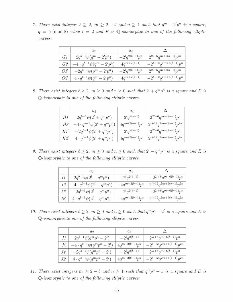
7. There exist integers ` ≥ 2, m ≥ 2 − b and n ≥ 1 such that qm − 2lpn is a square,
q ≡ 5 (mod 8) when l = 2 and E is Q-isomorphic to one of the following elliptic
curves:
a2 a4 ∆
G1 2qb−1ψ(qm − 2lpn) −2lq2(b−1)pn 22l+6qm+6(b−1)p2n
G2 −4 · qb−1ψ(qm − 2lpn) 4qm+2(b−1) −2l+12q2m+6(b−1)pn
G1′ −2qb−1ψ(qm − 2lpn) −2lq2(b−1)pn 22l+6qm+6(b−1)p2n
G2′ 4 · qb−1ψ(qm − 2lpn) 4qm+2(b−1) −2l+12q2m+6(b−1)pn
8. There exist integers ` ≥ 2, m ≥ 0 and n ≥ 0 such that 2l + qmpn is a square and E is
Q-isomorphic to one of the following elliptic curves
a2 a4 ∆
H1 2qb−1ψ(2l + qmpn) 2lq2(b−1) 22l+6qm+6(b−1)pn
H2 −4 · qb−1ψ(2l + qmpn) 4qm+2(b−1)pn 2l+12q2m+6(b−1)p2n
H1′ −2qb−1ψ(2l + qmpn) 2lq2(b−1) 22l+6qm+6(b−1)pn
H2′ 4 · qb−1ψ(2l + qmpn) 4qm+2(b−1)pn 2l+12q2m+6(b−1)p2n
9. There exist integers ` ≥ 2, m ≥ 0 and n ≥ 0 such that 2l − qmpn is a square and E is
Q-isomorphic to one of the following elliptic curves
a2 a4 ∆
I1 2qb−1ψ(2l − qmpn) 2lq2(b−1) −22l+6qm+6(b−1)pn
I2 −4 · qb−1ψ(2l − qmpn) −4qm+2(b−1)pn 2l+12q2m+6(b−1)p2n
I1′ −2qb−1ψ(2l − qmpn) 2lq2(b−1) −22l+6qm+6(b−1)pn
I2′ 4 · qb−1ψ(2l − qmpn) −4qm+2(b−1)pn 2l+12q2m+6(b−1)p2n
10. There exist integers ` ≥ 2, m ≥ 0 and n ≥ 0 such that qmpn − 2l is a square and E is
Q-isomorphic to one of the following elliptic curves
a2 a4 ∆
J1 2qb−1ψ(qmpn − 2l) −2lq2(b−1) 22l+6qm+6(b−1)pn
J2 −4 · qb−1ψ(qmpn − 2l) 4qm+2(b−1)pn −2l+12q2m+6(b−1)p2n
J1′ −2qb−1ψ(qmpn − 2l) −2lq2(b−1) 22l+6qm+6(b−1)pn
J2′ 4 · qb−1ψ(qmpn − 2l) 4qm+2(b−1)pn −2l+12q2m+6(b−1)p2n
11. There exist integers m ≥ 2 − b and n ≥ 1 such that qmpn + 1 is a square and E is
Q-isomorphic to one of the following elliptic curves:
65

a2 a4 ∆
K1 2qb−1ψ(qmpn + 1) q2(b−1) 26q2m+6(b−1)p2n
K2 −4 · qb−1ψ(qmpn + 1) 4qm+2(b−1)pn 212qm+6(b−1)pn
K1′ −2qb−1ψ(qmpn + 1) q2(b−1) 26q2m+6(b−1)p2n
K2′ 4 · qb−1ψ(qmpn + 1) 4qm+2(b−1)pn 212qm+6(b−1)pn
12. There exist integers m ≥ 2−b and n ≥ 1 such that qmpn−1 is a square, p ≡ 1 (mod 4),
q ≡ 1 (mod 4) if m > 0 and E is Q-isomorphic to one of the following elliptic curves:
a2 a4 ∆
L1 2qb−1ψ(qmpn − 1) qm+2(b−1)pn 26q2m+6(b−1)p2n
L2 −4 · qb−1ψ(qmpn − 1) 4q2(b−1) 212qm+6(b−1)pn
L1′ −2qb−1ψ(qmpn − 1) qm+2(b−1)pn 26q2m+6(b−1)p2n
L2′ 4 · qb−1ψ(qmpn − 1) 4q2(b−1) 212qm+6(b−1)pn
13. There exist integers m ≥ 2 − b and n ≥ 1 such that qm + pn is a square and E is
Q-isomorphic to one of the following elliptic curves:
(a) m is even or q ≡ 1 (mod 4);
a2 a4 ∆
M1 2qb−1ψ(qm + pn) qm+2(b−1) 26q2m+6(b−1)pn
M2 −4 · qb−1ψ(qm + pn) 4q2(b−1)pn 212qm+6(b−1)p2n
M1′ −2qb−1ψ(qm + pn) qm+2(b−1) 26q2m+6(b−1)pn
M2′ 4 · qb−1ψ(qm + pn) 4q2(b−1)pn 212qm+6(b−1)p2n
(b) m is odd and q ≡ 3 (mod 4);
a2 a4 ∆
N1 2qb−1ψ(qm + pn) q2(b−1)pn 26qm+6(b−1)p2n
N2 −4 · qb−1ψ(qm + pn) 4qm+2(b−1) 212q2m+6(b−1)pn
N1′ −2qb−1ψ(qm + pn) q2(b−1)pn 26qm+6(b−1)p2n
N2′ 4 · qb−1ψ(qm + pn) 4qm+2(b−1) 212q2m+6(b−1)pn
14. There exist integers m ≥ 2 − b and n ≥ 1 such that qm − pn is a square and E is
Q-isomorphic to one of the following elliptic curves:
(a) m is even or q ≡ 1 (mod 4);
66
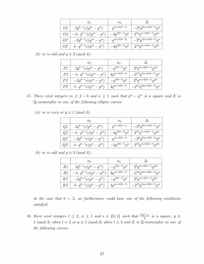
a2 a4 ∆
O1 2qb−1ψ(qm − pn) qm+2(b−1) −26q2m+6(b−1)pn
O2 −4 · qb−1ψ(qm − pn) −4q2(b−1)pn 212qm+6(b−1)p2n
O1′ −2qb−1ψ(qm − pn) qm+2(b−1) −26q2m+6(b−1)pn
O2′ 4 · qb−1ψ(qm − pn) −4q2(b−1)pn 212qm+6(b−1)p2n
(b) m is odd and q ≡ 3 (mod 4);
a2 a4 ∆
P1 2qb−1ψ(qm − pn) −q2(b−1)pn 26qm+6(b−1)p2n
P2 −4 · qb−1ψ(qm − pn) 4qm+2(b−1) −212q2m+6(b−1)pn
P1′ −2qb−1ψ(qm − pn) −q2(b−1)pn 26qm+6(b−1)p2n
P2′ 4 · qb−1ψ(qm − pn) 4qm+2(b−1) −212q2m+6(b−1)pn
15. There exist integers m ≥ 2 − b and n ≥ 1 such that pn − qm is a square and E is
Q-isomorphic to one of the following elliptic curves:
(a) m is even or q ≡ 1 (mod 4);
a2 a4 ∆
Q1 2qb−1ψ(pn − qm) qm+2(b−1) −26q2m+6(b−1)pn
Q2 −4 · qb−1ψ(pn − qm) −4q2(b−1)pn 212qm+6(b−1)p2n
Q1′ −2qb−1ψ(pn − qm) qm+2(b−1) −26q2m+6(b−1)pn
Q2′ 4 · qb−1ψ(pn − qm) −4q2(b−1)pn 212qm+6(b−1)p2n
(b) m is odd and q ≡ 3 (mod 4);
a2 a4 ∆
R1 2qb−1ψ(pn − qm) −q2(b−1)pn 26qm+6(b−1)p2n
R2 −4 · qb−1ψ(pn − qm) 4qm+2(b−1) −212q2m+6(b−1)pn
R1′ −2qb−1ψ(pn − qm) −q2(b−1)pn 26qm+6(b−1)p2n
R2′ 4 · qb−1ψ(pn − qm) 4qm+2(b−1) −212q2m+6(b−1)pn
In the case that b = 2, we furthermore could have one of the following conditions
satisfied:
16. there exist integers ` ≥ 2, n ≥ 1 and s ∈ 0, 1 such that 2lpn+1q
is a square, q ≡1 (mod 4) when l = 2 or q ≡ 1 (mod 8) when l ≥ 3 and E is Q-isomorphic to one of
the following curves:
67

a2 a4 ∆
S1 2qs+1ψ(2lpn+1q
) 2lq2s+1pn 22l+6q6s+3p2n
S2 −4 · qs+1ψ(2lpn+1q
) 4q2s+1 2l+12q6s+3pn
S1′ −2qs+1ψ(2lpn+1q
) 2lq2s+1pn 22l+6q6s+3p2n
S2′ 4 · qs+1ψ(2lpn+1q
) 4q2s+1 2l+12q6s+3pn
17. there exist integers ` ≥ 2, n ≥ 1 and s ∈ 0, 1 such that 2lpn−1q
is a square, q ≡3 (mod 4) when l = 2 or q ≡ 7 (mod 8) when l ≥ 3 and E is Q-isomorphic to one of
the following curves:
a2 a4 ∆
T1 2qs+1ψ(2lpn−1q
) 2lq2s+1pn −22l+6q6s+3p2n
T2 −4 · qs+1ψ(2lpn−1q
) −4q2s+1 2l+12q6s+3pn
T1′ −2qs+1ψ(2lpn−1q
) 2lq2s+1pn −22l+6q6s+3p2n
T2′ 4 · qs+1ψ(2lpn−1q
) −4q2s+1 2l+12q6s+3pn
18. there exist integers ` ≥ 2, n ≥ 1 and s ∈ 0, 1 such that 2l+pn
qis a square and E is
Q-isomorphic to one of the following curves:
a2 a4 ∆
U1 2qs+1ψ(2l+pn
q) 2lq2s+1 22l+6q6s+3pn
U2 −4 · qs+1ψ(2l+pn
q) 4q2s+1pn 2l+12q6s+3p2n
U1′ −2qs+1ψ(2l+pn
q) 2lq2s+1 22l+6q6s+3pn
U2′ 4 · qs+1ψ(2l+pn
q) 4q2s+1pn 2l+12q6s+3p2n
19. there exist integers ` ≥ 2, n ≥ 1 and s ∈ 0, 1 such that 2l−pnq
is a square and E is
Q-isomorphic to one of the following curves:
a2 a4 ∆
V1 2qs+1ψ(2l−pnq
) 2lq2s+1 −22l+6q6s+3pn
V2 −4 · qs+1ψ(2l−pnq
) −4q2s+1pn 2l+12q6s+3p2n
V1′ −2qs+1ψ(2l−pnq
) 2lq2s+1 −22l+6q6s+3pn
V2′ 4 · qs+1ψ(2l−pnq
) −4q2s+1pn 2l+12q6s+3p2n
20. there exist integers ` ≥ 2, n ≥ 1 and s ∈ 0, 1 such that pn−2l
qis a square and E is
Q-isomorphic to one of the following curves:
68

a2 a4 ∆
W1 2qs+1ψ(pn−2l
q) −2lq2s+1 22l+6q6s+3pn
W2 −4 · qs+1ψ(pn−2l
q) 4q2s+1pn −2l+12q6s+3p2n
W1′ −2qs+1ψ(pn−2l
q) −2lq2s+1 22l+6q6s+3pn
W2′ 4 · qs+1ψ(pn−2l
q) 4q2s+1pn −2l+12q6s+3p2n
21. there exist integers n ≥ 1 and s ∈ 0, 1 such that pn+1q
is a square, q ≡ 3 (mod 4) and
E is Q-isomorphic to one of the following curves:
a2 a4 ∆
X1 qs+1ψ(pn+1q
) q2s+1pn 26q6s+3p2n
X2 −2 · qs+1ψ(pn+1q
) 4q2s+1 212q6s+3pn
X1′ −qs+1ψ(pn+1q
) q2s+1pn 26q6s+3p2n
X2′ 2 · qs+1ψ(pn+1q
) 4q2s+1 212q6s+3pn
22. there exist integers n ≥ 1 and s ∈ 0, 1 such that pn+1q
is a square, q ≡ 1 (mod 4) and
E is Q-isomorphic to one of the following curves:
a2 a4 ∆
Y1 qs+1ψ(pn+1q
) q2s+1 26q6s+3pn
Y2 −2 · qs+1ψ(pn+1q
) 4q2s+1pn 212q6s+3p2n
Y1′ −qs+1ψ(pn+1q
) q2s+1 26q6s+3pn
Y2′ 2 · qs+1ψ(pn+1q
) 4q2s+1pn 212q6s+3p2n
23. there exist integers n ≥ 1 and s ∈ 0, 1 such that pn−1q
is a square, q ≡ 3 (mod 4) and
E is Q-isomorphic to one of the following curves:
a2 a4 ∆
Z1 qs+1ψ(pn−1q
) −q2s+1 26q6s+3pn
Z2 −2 · qs+1ψ(pn−1q
) 4q2s+1pn −212q6s+3p2n
Z1′ −qs+1ψ(pn−1q
) −q2s+1 26q6s+3pn
Z2′ 2 · qs+1ψ(pn−1q
) 4q2s+1pn −212q6s+3p2n
24. there exist integers n ≥ 1 and s ∈ 0, 1 such that pn−1q
is a square, q ≡ 1 (mod 4) and
E is Q-isomorphic to one of the following curves:
a2 a4 ∆
AA1 qs+1ψ(pn−1q
) q2s+1pn −26q6s+3p2n
AA2 −2 · qs+1ψ(pn−1q
) −4q2s+1 212q6s+3pn
AA1′ −qs+1ψ(pn−1q
) q2s+1pn −26q6s+3p2n
AA2′ 2 · qs+1ψ(pn−1q
) −4q2s+1 212q6s+3pn
69

Theorem 2.2.8. The elliptic curves E defined over Q of conductor 27qbp and having at least
one rational point of order 2 are the ones such that one of the following conditions is satisfied:
1. There exist integers m ≥ 2 − b and n ≥ 1 such that 2qmpn − 1 is a square, p, q ≡1 (mod 4), t ∈ 0, 1 and E is Q-isomorphic to one of the following elliptic curves:
a2 a4 ∆
A1 2t+1qb−1ψ(2qmpn − 1) 21+2tqm+2(b−1)pn −28+6tq2m+6(b−1)p2n
A2 −22−t · qb−1ψ(2qmpn − 1) −22−2tq2(b−1) 213−6tqm+6(b−1)pn
A1′ −2t+1qb−1ψ(2qmpn − 1) 21+2tqm+2(b−1)pn −28+6tq2m+6(b−1)p2n
A2′ 22−t · qb−1ψ(2qmpn − 1) −22−2tq2(b−1) 213−6tqm+6(b−1)pn
2. There exist integers m ≥ 2−b and n ≥ 1 such that 2qm+pn is a square, p ≡ 3 (mod 4),
n odd, t ∈ 0, 1 and E is Q-isomorphic to one of the following elliptic curves:
a2 a4 ∆
B1 2t+1qb−1ψ(2qm + pn) 21+2tqm+2(b−1) 28+6tq2m+6(b−1)pn
B2 −22−t · qb−1ψ(2qm + pn) 22−2tq2(b−1)pn 213−6tqm+6(b−1)p2n
B1′ −2t+1qb−1ψ(2qm + pn) 21+2tqm+2(b−1) 28+6tq2m+6(b−1)pn
B2′ 22−t · qb−1ψ(2qm + pn) 22−2tq2(b−1)pn 213−6tqm+6(b−1)p2n
3. There exist integers m ≥ 2− b and n ≥ 1 such that 2qm − pn is a square, n is even or
p ≡ 1 (mod 4), t ∈ 0, 1 and E is Q-isomorphic to one of the following elliptic curves:
a2 a4 ∆
C1 2t+1qb−1ψ(2qm − pn) 21+2tqm+2(b−1) −28+6tq2m+6(b−1)pn
C2 −22−t · qb−1ψ(2qm − pn) −22−2tq2(b−1)pn 213−6tqm+6(b−1)p2n
C1′ −2t+1qb−1ψ(2qm − pn) 21+2tqm+2(b−1) −28+6tq2m+6(b−1)pn
C2′ 22−t · qb−1ψ(2qm − pn) −22−2tq2(b−1)pn 213−6tqm+6(b−1)p2n
4. There exist integers m ≥ 2−b and n ≥ 1 such that pn−2qm is a square, p ≡ 3 (mod 4),
n odd, t ∈ 0, 1 and E is Q-isomorphic to one of the following elliptic curves:
a2 a4 ∆
D1 2t+1qb−1ψ(pn − 2qm) −21+2tqm+2(b−1) 28+6tq2m+6(b−1)pn
D2 −22−t · qb−1ψ(pn − 2qm) 22−2tq2(b−1)pn −213−6tqm+6(b−1)p2n
D1′ −2t+1qb−1ψ(pn − 2qm) −21+2tqm+2(b−1) 28+6tq2m+6(b−1)pn
D2′ 22−t · qb−1ψ(pn − 2qm) 22−2tq2(b−1)pn −213−6tqm+6(b−1)p2n
70

5. There exist integers m ≥ 2− b and n ≥ 1 such that 2pn + qm is a square, t ∈ 0, 1 and
E is Q-isomorphic to one of the following elliptic curves:
a2 a4 ∆
E1 2t+1qb−1ψ(2pn + qm) 21+2tq2(b−1)pn 28+6tqm+6(b−1)p2n
E2 −22−t · qb−1ψ(2pn + qm) 22−2tqm+2(b−1) 213−6tq2m+6(b−1)pn
E1′ −2t+1qb−1ψ(2pn + qm) 21+2tq2(b−1)pn 28+6tqm+6(b−1)p2n
E2′ 22−t · qb−1ψ(2pn + qm) 22−2tqm+2(b−1) 213−6tq2m+6(b−1)pn
6. There exist integers m ≥ 2− b and n ≥ 1 such that 2pn− qm is a square, t ∈ 0, 1 and
E is Q-isomorphic to one of the following elliptic curves:
a2 a4 ∆
F1 2t+1qb−1ψ(2pn − qm) 21+2tq2(b−1)pn −28+6tqm+6(b−1)p2n
F2 −22−t · qb−1ψ(2pn − qm) −22−2tqm+2(b−1) 213−6tq2m+6(b−1)pn
F1′ −2t+1qb−1ψ(2pn − qm) 21+2tq2(b−1)pn −28+6tqm+6(b−1)p2n
F2′ 22−t · qb−1ψ(2pn − qm) −22−2tqm+2(b−1) 213−6tq2m+6(b−1)pn
7. There exist integers m ≥ 2− b and n ≥ 1 such that qm− 2pn is a square, t ∈ 0, 1 and
E is Q-isomorphic to one of the following elliptic curves:
a2 a4 ∆
G1 2t+1qb−1ψ(qm − 2pn) −21+2tq2(b−1)pn 28+6tqm+6(b−1)p2n
G2 −22−t · qb−1ψ(qm − 2pn) 22−2tqm+2(b−1) −213−6tq2m+6(b−1)pn
G1′ −2t+1qb−1ψ(qm − 2pn) −21+2tq2(b−1)pn 28+6tqm+6(b−1)p2n
G2′ 22−t · qb−1ψ(qm − 2pn) 22−2tqm+2(b−1) −213−6tq2m+6(b−1)pn
8. There exist integers m ≥ 2 − b and n ≥ 1 such that 2 + qmpn is a square, p ≡ 1 or
7 (mod 8), q ≡ 1 or 7 (mod 8) if m > 0, t ∈ 0, 1 and E is Q-isomorphic to one of
the following elliptic curves:
a2 a4 ∆
H1 2t+1qb−1ψ(2 + qmpn) 21+2tq2(b−1) 28+6tqm+6(b−1)p2n
H2 −22−t · qb−1ψ(2 + qmpn) 22−2tqm+2(b−1)pn 213−6tq2m+6(b−1)pn
H1′ −2t+1qb−1ψ(2 + qmpn) 21+2tq2(b−1) 28+6tqm+6(b−1)p2n
H2′ 22−t · qb−1ψ(2 + qmpn) 22−2tqm+2(b−1)pn 213−6tq2m+6(b−1)pn
9. There exist integers m ≥ 2 − b and n ≥ 1 such that qmpn − 2 is a square, p ≡ 1 or
3 (mod 8), q ≡ 1 or 3 (mod 8) if m > 0, t ∈ 0, 1 and E is Q-isomorphic to one of
the following elliptic curves:
71

a2 a4 ∆
I1 2t+1qb−1ψ(qmpn − 2) −21+2tq2(b−1) 28+6tqm+6(b−1)p2n
I2 −22−t · qb−1ψ(qmpn − 2) 22−2tqm+2(b−1)pn −213−6tq2m+6(b−1)pn
I1′ −2t+1qb−1ψ(qmpn − 2) −21+2tq2(b−1) 28+6tqm+6(b−1)p2n
I2′ 22−t · qb−1ψ(qmpn − 2) 22−2tqm+2(b−1)pn −213−6tq2m+6(b−1)pn
In the case that b = 2, we furthermore could have one of the following conditions
satisfied:
10. there exist integers n ≥ 1 and s ∈ 0, 1 such that 2pn+1q
is a square, q ≡ 3 (mod 4),
t ∈ 0, 1 and E is Q-isomorphic to one of the following curves:
a2 a4 ∆
J1 2t+1qs+1ψ(2pn+1q
) 21+2tq2s+1pn 28+6tq6s+3p2n
J2 −22−t · qs+1ψ(2pn+1q
) 22−2tq2s+1 213−6tq6s+3pn
J1′ −2t+1qs+1ψ(2pn+1q
) 21+2tq2s+1pn 28+6tq6s+3p2n
J2′ 22−t · qs+1ψ(2pn+1q
) 22−2tq2s+1 213−6tq6s+3pn
11. there exist integers n ≥ 1 and s ∈ 0, 1 such that 2pn−1q
is a square, q ≡ 1 (mod 4),
t ∈ 0, 1 and E is Q-isomorphic to one of the following curves:
a2 a4 ∆
K1 2t+1qs+1ψ(2pn−1q
) 21+2tq2s+1pn −28+6tq6s+3p2n
K2 −22−t · qs+1ψ(2pn−1q
) −22−2tq2s+1 213−6tq6s+3pn
K1′ −2t+1qs+1ψ(2pn−1q
) 21+2tq2s+1pn −28+6tq6s+3p2n
K2′ 22−t · qs+1ψ(2pn−1q
) −22−2tq2s+1 213−6tq6s+3pn
12. there exist integers n ≥ 1 and s ∈ 0, 1 such that 2+pn
qis a square, t ∈ 0, 1 and E is
Q-isomorphic to one of the following curves:
a2 a4 ∆
L1 2t+1qb−1ψ(2+pn
q) 21+2tq2(b−1) 28+6tq6s+3pn
L2 −22−t · qb−1ψ(2+pn
q) 22−2tq2(b−1)pn 213−6tq6s+3p2n
L1′ −2t+1qb−1ψ(2+pn
q) 21+2tq2(b−1) 28+6tq6s+3pn
L2′ 22−t · qb−1ψ(2+pn
q) 22−2tq2(b−1)pn 213−6tq6s+3p2n
13. there exist integers n ≥ 1 and s ∈ 0, 1 such that pn−2q
is a square, t ∈ 0, 1 and E is
Q-isomorphic to one of the following curves:
72
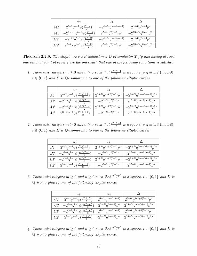
a2 a4 ∆
M1 2t+1qb−1ψ(pn−2q
) −21+2tqm+2(b−1) 28+6tq6s+3pn
M2 −22−t · qb−1ψ(pn−2q
) 22−2tq2(b−1)pn −213−6tq6s+3p2n
M1′ −2t+1qb−1ψ(pn−2q
) −21+2tqm+2(b−1) 28+6tq6s+3pn
M2′ 22−t · qb−1ψ(pn−2q
) 22−2tq2(b−1)pn −213−6tq6s+3p2n
Theorem 2.2.9. The elliptic curves E defined over Q of conductor 28qbp and having at least
one rational point of order 2 are the ones such that one of the following conditions is satisfied:
1. There exist integers m ≥ 0 and n ≥ 0 such that qmpn+12
is a square, p, q ≡ 1, 7 (mod 8),
t ∈ 0, 1 and E is Q-isomorphic to one of the following elliptic curves
a2 a4 ∆
A1 2t+2qb−1ψ( qmpn+1
2) 21+2tqm+2(b−1)pn −29+6tq2m+6(b−1)p2n
A2 −23−tqb−1ψ( qmpn+1
2) −23−2tq2(b−1) 215−6tqm+6(b−1)pn
A1′ −2t+2qb−1ψ( qmpn+1
2) 21+2tqm+2(b−1)pn −29+6tq2m+6(b−1)p2n
A2′ 23−tqb−1ψ( qmpn+1
2) −23−2tq2(b−1) 215−6tqm+6(b−1)pn
2. There exist integers m ≥ 0 and n ≥ 0 such that qmpn−12
is a square, p, q ≡ 1, 3 (mod 8),
t ∈ 0, 1 and E is Q-isomorphic to one of the following elliptic curves
a2 a4 ∆
B1 2t+2qb−1ψ( qmpn−1
2) 21+2tqm+2(b−1)pn −29+6tq2m+6(b−1)p2n
B2 −23−tqb−1ψ( qmpn−1
2) −23−2tq2(b−1) 215−6tqm+6(b−1)pn
B1′ −2t+2qb−1ψ( qmpn−1
2) 21+2tqm+2(b−1)pn −29+6tq2m+6(b−1)p2n
B2′ 23−tqb−1ψ( qmpn−1
2) −23−2tq2(b−1) 215−6tqm+6(b−1)pn
3. There exist integers m ≥ 0 and n ≥ 0 such that qm+pn
2is a square, t ∈ 0, 1 and E is
Q-isomorphic to one of the following elliptic curves
a2 a4 ∆
C1 2t+2qb−1ψ( qm+pn
2) 21+2tqm+2(b−1) 29+6tq2m+6(b−1)pn
C2 −23−tqb−1ψ( qm+pn
2) 23−2tq2(b−1)pn 215−6tqm+6(b−1)p2n
C1′ −2t+2qb−1ψ( qm+pn
2) 21+2tqm+2(b−1) 29+6tq2m+6(b−1)pn
C2′ 23−tqb−1ψ( qm+pn
2) 23−2tq2(b−1)pn 215−6tqm+6(b−1)p2n
4. There exist integers m ≥ 0 and n ≥ 0 such that qm−pn2
is a square, t ∈ 0, 1 and E is
Q-isomorphic to one of the following elliptic curves
73

a2 a4 ∆
D1 2t+2qb−1ψ( qm−pn
2) 21+2tqm+2(b−1) −29+6tq2m+6(b−1)pn
D2 −23−tqb−1ψ( qm−pn
2) −23−2tq2(b−1)pn 215−6tqm+6(b−1)p2n
D1′ −2t+2qb−1ψ( qm−pn
2) 21+2tqm+2(b−1) −29+6tq2m+6(b−1)pn
D2′ 23−tqb−1ψ( qm−pn
2) −23−2tq2(b−1)pn 215−6tqm+6(b−1)p2n
5. There exist integers m ≥ 0 and n ≥ 0 such that pn−qm2
is a square, t ∈ 0, 1 and E is
Q-isomorphic to one of the following elliptic curves
a2 a4 ∆
E1 2t+2qb−1ψ(pn−qm
2) 21+2tq2(b−1)pn −29+6tqm+6(b−1)p2n
E2 −23−tqb−1ψ(pn−qm
2) −23−2tqm+2(b−1) 215−6tq2m+6(b−1)pn
E1′ −2t+2qb−1ψ(pn−qm
2) 21+2tq2(b−1)pn −29+6tqm+6(b−1)p2n
E2′ 23−tqb−1ψ(pn−qm
2) −23−2tqm+2(b−1) 215−6tq2m+6(b−1)pn
In the case that b = 2, we furthermore could have one of the following conditions
satisfied:
6. There exist integers m ≥ 0 and n ≥ 0 such that pn+12q
is a square, pn ≡ 1 (mod 4),
s, t ∈ 0, 1 and E is Q-isomorphic to one of the following elliptic curves
a2 a4 ∆
F1 2t+2qs+1pψ(pn+1q
) 21+2tq2s+1pn 29+6tq6s+3p2n
F2 −23−tqs+1pψ(pn+1q
) 23−2tq2s+1 215−6tq6s+3pn
F1′ −2t+2qs+1pψ(pn+1q
) 21+2tq2s+1pn 29+6tq6s+3p2n
F2′ 23−tqs+1pψ(pn+1q
) 23−2tq2s+1 215−6tq6s+3pn
7. There exist integers m ≥ 0 and n ≥ 0 such that pn−12q
is a square, pn ≡ 3 (mod 4),
s, t ∈ 0, 1 and E is Q-isomorphic to one of the following elliptic curves
a2 a4 ∆
G1 2t+2qs+1pψ(pn+1q
) 21+2tq2s+1pn −29+6tq6s+3p2n
G2 −23−tqs+1pψ(pn+1q
) −23−2tq2s+1 215−6tq6s+3pn
G1′ −2t+2qs+1pψ(pn+1q
) 21+2tq2s+1pn −29+6tq6s+3p2n
G2′ 23−tqs+1pψ(pn+1q
) −23−2tq2s+1 215−6tq6s+3pn
Theorem 2.2.10. The elliptic curves E defined over Q of conductor q2p2 and having at
least one rational point of order 2 are the ones such that one of the following conditions is
satisfied:
74
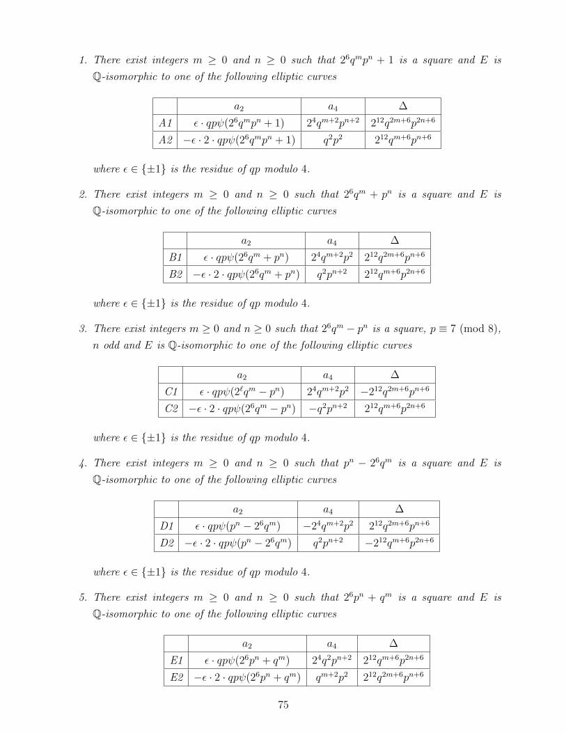
1. There exist integers m ≥ 0 and n ≥ 0 such that 26qmpn + 1 is a square and E is
Q-isomorphic to one of the following elliptic curves
a2 a4 ∆
A1 ε · qpψ(26qmpn + 1) 24qm+2pn+2 212q2m+6p2n+6
A2 −ε · 2 · qpψ(26qmpn + 1) q2p2 212qm+6pn+6
where ε ∈ ±1 is the residue of qp modulo 4.
2. There exist integers m ≥ 0 and n ≥ 0 such that 26qm + pn is a square and E is
Q-isomorphic to one of the following elliptic curves
a2 a4 ∆
B1 ε · qpψ(26qm + pn) 24qm+2p2 212q2m+6pn+6
B2 −ε · 2 · qpψ(26qm + pn) q2pn+2 212qm+6p2n+6
where ε ∈ ±1 is the residue of qp modulo 4.
3. There exist integers m ≥ 0 and n ≥ 0 such that 26qm − pn is a square, p ≡ 7 (mod 8),
n odd and E is Q-isomorphic to one of the following elliptic curves
a2 a4 ∆
C1 ε · qpψ(2`qm − pn) 24qm+2p2 −212q2m+6pn+6
C2 −ε · 2 · qpψ(26qm − pn) −q2pn+2 212qm+6p2n+6
where ε ∈ ±1 is the residue of qp modulo 4.
4. There exist integers m ≥ 0 and n ≥ 0 such that pn − 26qm is a square and E is
Q-isomorphic to one of the following elliptic curves
a2 a4 ∆
D1 ε · qpψ(pn − 26qm) −24qm+2p2 212q2m+6pn+6
D2 −ε · 2 · qpψ(pn − 26qm) q2pn+2 −212qm+6p2n+6
where ε ∈ ±1 is the residue of qp modulo 4.
5. There exist integers m ≥ 0 and n ≥ 0 such that 26pn + qm is a square and E is
Q-isomorphic to one of the following elliptic curves
a2 a4 ∆
E1 ε · qpψ(26pn + qm) 24q2pn+2 212qm+6p2n+6
E2 −ε · 2 · qpψ(26pn + qm) qm+2p2 212q2m+6pn+6
75

where ε ∈ ±1 is the residue of qp modulo 4.
6. There exist integers m ≥ 0 and n ≥ 0 such that 26pn − qm is a square, q ≡ 7 (mod 8),
m odd and E is Q-isomorphic to one of the following elliptic curves
a2 a4 ∆
F1 ε · qpψ(26pn − qm) 24q2pn+2 −212qm+6p2n+6
F2 −ε · 2 · qpψ(26pn − qm) −qm+2p2 212q2m+6pn+6
where ε ∈ ±1 is the residue of qp modulo 4.
7. There exist integers ` ≥ 7, m ≥ 0 and n ≥ 0 such that qm − 26pn is a square and E is
Q-isomorphic to one of the following elliptic curves
a2 a4 ∆
G1 ε · qpψ(qm − 26pn) −24q2pn+2 212qm+6p2n+6
G2 −ε · 2 · qpψ(qm − 26pn) qm+2p2 −212q2m+6pn+6
where ε ∈ ±1 is the residue of qp modulo 4.
8. There exist integers m ≥ 0 and n ≥ 0 such that 26 + qmpn is a square and E is
Q-isomorphic to one of the following elliptic curves
a2 a4 ∆
H1 ε · qpψ(26 + qmpn) 24q2p2 212qm+6pn+6
H2 −ε · 2 · qpψ(26 + qmpn) qm+2pn+2 212q2m+6p2n+6
where ε ∈ ±1 is the residue of qp modulo 4.
9. There exist integers m ≥ 0 and n ≥ 0 such that 26 − qmpn is a square and E is
Q-isomorphic to one of the following elliptic curves
a2 a4 ∆
I1 ε · qpψ(26 − qmpn) 24q2p2 −212qm+6pn+6
I2 −ε · 2 · qpψ(26 − qmpn) −qm+2pn+2 212q2m+6p2n+6
where ε ∈ ±1 is the residue of qp modulo 4.
10. There exist integers m ≥ 0 and n ≥ 0 such that qmpn − 26 is a square and E is
Q-isomorphic to one of the following elliptic curves
76

a2 a4 ∆
J1 ε · qpψ(qmpn − 26) −24q2p2 212qm+6pn+6
J2 −ε · 2 · qpψ(qmpn − 26) qm+2pn+2 −212q2m+6p2n+6
where ε ∈ ±1 is the residue of qp modulo 4.
11. There exist integers m ≥ 0 and r ∈ 0, 1 such that 26qm+1p
is a square, p ≡ 1 (mod 8)
and E is Q-isomorphic to one of the following elliptic curves
a2 a4 ∆
K1 ε · qpr+1ψ(26qm+1p
) 24qm+2p2r+1 212q2m+6p6r+3
K2 −ε · 2 · qpr+1ψ(26qm+1p
) q2p2r+1 212qm+6p6r+3
where ε ∈ ±1 is the residue of q modulo 4.
12. There exist integers m ≥ 0 and r ∈ 0, 1 such that 26qm−1p
is a square, p ≡ 7 (mod 8)
and E is Q-isomorphic to one of the following elliptic curves
a2 a4 ∆
L1 ε · qpr+1ψ(26qm−1p
) 24qm+2p2r+1 −212q2m+6p6r+3
L2 −ε · 2 · qpr+1ψ(26qm−1p
) −q2p2r+1 212qm+6p6r+3
where ε ∈ ±1 is the residue of qpr+1 modulo 4.
13. There exist integers m ≥ 0 and r ∈ 0, 1 such that 26+qm
pis a square and E is Q-
isomorphic to one of the following elliptic curves
a2 a4 ∆
M1 ε · qpr+1ψ(26+qm
p) 24q2p2r+1 212qm+6p6r+3
M2 −ε · 2 · qpr+1ψ(26+qm
p) qm+2p2r+1 212q2m+6p6r+3
where ε ∈ ±1 is the residue of qpr+1 modulo 4.
14. There exist integers m ≥ 0 and r ∈ 0, 1 such that 26−qmp
is a square and E is Q-
isomorphic to one of the following elliptic curves
a2 a4 ∆
N1 ε · qpr+1ψ(26−qmp
) 24q2p2r+1 −212qm+6p6r+3
N2 −ε · 2 · qpr+1ψ(26−qmp
) −qm+2p2r+1 212q2m+6p6r+3
where ε ∈ ±1 is the residue of qpr+1 modulo 4.
77

15. There exist integers m ≥ 0 and r ∈ 0, 1 such that qm−26
pis a square and E is Q-
isomorphic to one of the following elliptic curves
a2 a4 ∆
O1 ε · qpr+1ψ( qm−26
p) −24q2p2r+1 212qm+6p6r+3
O2 −ε · 2 · qpr+1ψ( qm−26
p) qm+2p2r+1 −212q2m+6p6r+3
where ε ∈ ±1 is the residue of qpr+1 modulo 4.
16. There exist integers n ≥ 0 and s ∈ 0, 1 such that 26pn+1q
is a square, q ≡ 1 (mod 8)
and E is Q-isomorphic to one of the following elliptic curves
a2 a4 ∆
P1 ε · qs+1pψ(26pn+1q
) 24q2s+1pn+2 212q6s+3p2n+6
P2 −ε · 2 · qs+1pψ(26pn+1q
) q2s+1p2 212q6s+3pn+6
where ε ∈ ±1 is the residue of p modulo 4.
17. There exist integers n ≥ 0 and s ∈ 0, 1 such that 26pn−1q
is a square, q ≡ 7 (mod 8)
and E is Q-isomorphic to one of the following elliptic curves
a2 a4 ∆
Q1 ε · qs+1pψ(26pn−1q
) 24q2s+1pn+2 −212q6s+3p2n+6
Q2 −ε · 2 · qs+1pψ(26pn−1q
) −q2s+1p2 212q6s+3pn+6
where ε ∈ ±1 is the residue of qs+1p modulo 4.
18. There exist integers n ≥ 0 and s ∈ 0, 1 such that 26+pn
qis a square and E is Q-
isomorphic to one of the following elliptic curves
a2 a4 ∆
R1 ε · qs+1pψ(26+pn
q) 24q2s+1p2 212q6s+3pn+6
R2 −ε · 2 · qs+1pψ(26+pn
q) q2s+1pn+2 212q6s+3p2n+6
where ε ∈ ±1 is the residue of qs+1p modulo 4.
19. There exist integers n ≥ 0 and s ∈ 0, 1 such that 26−pnq
is a square and E is Q-
isomorphic to one of the following elliptic curve
a2 a4 ∆
S1 ε · qs+1pψ(26−pnq
) 24q2s+1p2 −212q6s+3pn+6
S2 −ε · 2 · qs+1pψ(26−pnq
) −q2s+1pn+2 212q6s+3p2n+6
78

where ε ∈ ±1 is the residue of qs+1p modulo 4.
20. There exist integers n ≥ 0 and s ∈ 0, 1 such that pn−26
qis a square and E is Q-
isomorphic to one of the following elliptic curve
a2 a4 ∆
T1 ε · qs+1pψ(pn−26
q) −24q2s+1p2 212q6s+3pn+6
T2 −ε · 2 · qs+1pψ(pn−26
q) q2s+1pn+2 −212q6s+3p2n+6
where ε ∈ ±1 is the residue of qs+1p modulo 4.
21. There exist integers r, s ∈ 0, 1 such that 26+1qp
is a square and E is Q-isomorphic to
one of the following elliptic curve
a2 a4 ∆
U1 ε · qs+1pr+1ψ(26+1qp
) 24q2s+1p2r+1 212q6s+3p6r+3
U2 −ε · 2 · qs+1pr+1ψ(26+1qp
) q2s+1p2r+1 212q6s+3p6r+3
where ε ∈ ±1 is the residue of qs+1pr+1 modulo 4.
22. There exist integers r, s ∈ 0, 1 such that 26−1qp
is a square and E is Q-isomorphic to
one of the following elliptic curve
a2 a4 ∆
V1 ε · qs+1pr+1ψ(26−1qp
) 24q2s+1p2r+1 −212q6s+3p6r+3
V2 −ε · 2 · qs+1pr+1ψ(26−1qp
) −q2s+1p2r+1 212q6s+3p6r+3
where ε ∈ ±1 is the residue of qs+1pr+1 modulo 4.
Theorem 2.2.11. The elliptic curves E defined over Q of conductor 2q2p2 and having at
least one rational point of order 2 are the ones such that one of the following conditions is
satisfied:
1. There exist integers ` ≥ 7, m ≥ 0 and n ≥ 0 such that 2`qmpn + 1 is a square and E is
Q-isomorphic to one of the following elliptic curves
a2 a4 ∆
A1 ε · qpψ(2`qmpn + 1) 2`−2qm+2pn+2 22`q2m+6p2n+6
A2 −ε · 2 · qpψ(2`qmpn + 1) q2p2 2`+6qm+6pn+6
where ε ∈ ±1 is the residue of qp modulo 4.
79

2. There exist integers ` ≥ 7, m ≥ 0 and n ≥ 0 such that 2`qm + pn is a square and E is
Q-isomorphic to one of the following elliptic curves
a2 a4 ∆
B1 ε · qpψ(2`qm + pn) 2`−2qm+2p2 22`q2m+6pn+6
B2 −ε · 2 · qpψ(2`qm + pn) q2pn+2 2`+6qm+6p2n+6
where ε ∈ ±1 is the residue of qp modulo 4.
3. There exist integers ` ≥ 7, m ≥ 0 and n ≥ 0 such that 2`qm − pn is a square, p ≡7 (mod 8), n odd and E is Q-isomorphic to one of the following elliptic curves
a2 a4 ∆
C1 ε · qpψ(2`qm − pn) 2`−2qm+2p2 −22`q2m+6pn+6
C2 −ε · 2 · qpψ(2`qm − pn) −q2pn+2 2`+6qm+6p2n+6
where ε ∈ ±1 is the residue of qp modulo 4.
4. There exist integers ` ≥ 7, m ≥ 0 and n ≥ 0 such that pn − 2`qm is a square and E is
Q-isomorphic to one of the following elliptic curves
a2 a4 ∆
D1 ε · qpψ(pn − 2`qm) −2`−2qm+2p2 22`q2m+6pn+6
D2 −ε · 2 · qpψ(pn − 2`qm) q2pn+2 −2`+6qm+6p2n+6
where ε ∈ ±1 is the residue of qp modulo 4.
5. There exist integers ` ≥ 7, m ≥ 0 and n ≥ 0 such that 2`pn + qm is a square and E is
Q-isomorphic to one of the following elliptic curves
a2 a4 ∆
E1 ε · qpψ(2`pn + qm) 2`−2q2pn+2 22`qm+6p2n+6
E2 −ε · 2 · qpψ(2`pn + qm) qm+2p2 2`+6q2m+6pn+6
where ε ∈ ±1 is the residue of qp modulo 4.
6. There exist integers ` ≥ 7, m ≥ 0 and n ≥ 0 such that 2`pn − qm is a square, q ≡7 (mod 8), m odd and E is Q-isomorphic to one of the following elliptic curves
a2 a4 ∆
F1 ε · qpψ(2`pn − qm) 2`−2q2pn+2 −22`qm+6p2n+6
F2 −ε · 2 · qpψ(2`pn − qm) −qm+2p2 2`+6q2m+6pn+6
80

where ε ∈ ±1 is the residue of qp modulo 4.
7. There exist integers ` ≥ 7, m ≥ 0 and n ≥ 0 such that qm − 2`pn is a square and E is
Q-isomorphic to one of the following elliptic curves
a2 a4 ∆
G1 ε · qpψ(qm − 2`pn) −2`−2q2pn+2 22`qm+6p2n+6
G2 −ε · 2 · qpψ(qm − 2`pn) qm+2p2 −2`+6q2m+6pn+6
where ε ∈ ±1 is the residue of qp modulo 4.
8. There exist integers ` ≥ 7, m ≥ 0 and n ≥ 0 such that 2` + qmpn is a square and E is
Q-isomorphic to one of the following elliptic curves
a2 a4 ∆
H1 ε · qpψ(2` + qmpn) 2`−2q2p2 22`qm+6pn+6
H2 −ε · 2 · qpψ(2` + qmpn) qm+2pn+2 2`+6q2m+6p2n+6
where ε ∈ ±1 is the residue of qp modulo 4.
9. There exist integers ` ≥ 7, m ≥ 0 and n ≥ 0 such that 2` − qmpn is a square and E is
Q-isomorphic to one of the following elliptic curves
a2 a4 ∆
I1 ε · qpψ(2` − qmpn) 2`−2q2p2 −22`qm+6pn+6
I2 −ε · 2 · qpψ(2` − qmpn) −qm+2pn+2 2`+6q2m+6p2n+6
where ε ∈ ±1 is the residue of qp modulo 4.
10. There exist integers ` ≥ 7, m ≥ 0 and n ≥ 0 such that qmpn − 2` is a square and E is
Q-isomorphic to one of the following elliptic curves
a2 a4 ∆
J1 ε · qpψ(qmpn − 2`) −2`−2q2p2 22`qm+6pn+6
J2 −ε · 2 · qpψ(qmpn − 2`) qm+2pn+2 −2`+6q2m+6p2n+6
where ε ∈ ±1 is the residue of qp modulo 4.
11. There exist integers ` ≥ 7, m ≥ 0 and r ∈ 0, 1 such that 2`qm+1p
is a square, p ≡1 (mod 8) and E is Q-isomorphic to one of the following elliptic curves
81

a2 a4 ∆
K1 ε · qpr+1ψ(2`qm+1p
) 2`−2qm+2p2r+1 22`q2m+6p6r+3
K2 −ε · 2 · qpr+1ψ(2`qm+1p
) q2p2r+1 2`+6qm+6p6r+3
where ε ∈ ±1 is the residue of q modulo 4.
12. There exist integers ` ≥ 7, m ≥ 0 and r ∈ 0, 1 such that 2`qm−1p
is a square, p ≡7 (mod 8) and E is Q-isomorphic to one of the following elliptic curves
a2 a4 ∆
L1 ε · qpr+1ψ(2`qm−1p
) 2`−2qm+2p2r+1 −22`q2m+6p6r+3
L2 −ε · 2 · qpr+1ψ(2`qm−1p
) −q2p2r+1 2`+6qm+6p6r+3
where ε ∈ ±1 is the residue of qpr+1 modulo 4.
13. There exist integers ` ≥ 7, m ≥ 0 and r ∈ 0, 1 such that 2`+qm
pis a square and E is
Q-isomorphic to one of the following elliptic curves
a2 a4 ∆
M1 ε · qpr+1ψ(2`+qm
p) 2`−2q2p2r+1 22`qm+6p6r+3
M2 −ε · 2 · qpr+1ψ(2`+qm
p) qm+2p2r+1 2`+6q2m+6p6r+3
where ε ∈ ±1 is the residue of qpr+1 modulo 4.
14. There exist integers ` ≥ 7, m ≥ 0 and r ∈ 0, 1 such that 2`−qmp
is a square and E is
Q-isomorphic to one of the following elliptic curves
a2 a4 ∆
N1 ε · qpr+1ψ(2`−qmp
) 2`−2q2p2r+1 −22`qm+6p6r+3
N2 −ε · 2 · qpr+1ψ(2`−qmp
) −qm+2p2r+1 2`+6q2m+6p6r+3
where ε ∈ ±1 is the residue of qpr+1 modulo 4.
15. There exist integers ` ≥ 7, m ≥ 0 and r ∈ 0, 1 such that qm−2`
pis a square and E is
Q-isomorphic to one of the following elliptic curves
a2 a4 ∆
O1 ε · qpr+1ψ( qm−2`
p) −2`−2q2p2r+1 22`qm+6p6r+3
O2 −ε · 2 · qpr+1ψ( qm−2`
p) qm+2p2r+1 −2`+6q2m+6p6r+3
where ε ∈ ±1 is the residue of qpr+1 modulo 4.
82

16. There exist integers ` ≥ 7, n ≥ 0 and s ∈ 0, 1 such that 2`pn+1q
is a square, q ≡1 (mod 8) and E is Q-isomorphic to one of the following elliptic curves
a2 a4 ∆
P1 ε · qs+1pψ(2`pn+1q
) 2`−2q2s+1pn+2 22`q6s+3p2n+6
P2 −ε · 2 · qs+1pψ(2`pn+1q
) q2s+1p2 2`+6q6s+3pn+6
where ε ∈ ±1 is the residue of p modulo 4.
17. There exist integers ` ≥ 7, n ≥ 0 and s ∈ 0, 1 such that 2`pn−1q
is a square, q ≡7 (mod 8) and E is Q-isomorphic to one of the following elliptic curves
a2 a4 ∆
Q1 ε · qs+1pψ(2`pn−1q
) 2`−2q2s+1pn+2 −22`q6s+3p2n+6
Q2 −ε · 2 · qs+1pψ(2`pn−1q
) −q2s+1p2 2`+6q6s+3pn+6
where ε ∈ ±1 is the residue of qs+1p modulo 4.
18. There exist integers ` ≥ 7, n ≥ 0 and s ∈ 0, 1 such that 2`+pn
qis a square and E is
Q-isomorphic to one of the following elliptic curves
a2 a4 ∆
R1 ε · qs+1pψ(2`+pn
q) 2`−2q2s+1p2 22`q6s+3pn+6
R2 −ε · 2 · qs+1pψ(2`+pn
q) q2s+1pn+2 2`+6q6s+3p2n+6
where ε ∈ ±1 is the residue of qs+1p modulo 4.
19. There exist integers ` ≥ 7, n ≥ 0 and s ∈ 0, 1 such that 2`−pnq
is a square and E is
Q-isomorphic to one of the following elliptic curve
a2 a4 ∆
S1 ε · qs+1pψ(2`−pnq
) 2`−2q2s+1p2 −22`q6s+3pn+6
S2 −ε · 2 · qs+1pψ(2`−pnq
) −q2s+1pn+2 2`+6q6s+3p2n+6
where ε ∈ ±1 is the residue of qs+1p modulo 4.
20. There exist integers ` ≥ 7, n ≥ 0 and s ∈ 0, 1 such that pn−2`
qis a square and E is
Q-isomorphic to one of the following elliptic curve
a2 a4 ∆
T1 ε · qs+1pψ(pn−2`
q) −2`−2q2s+1p2 22`q6s+3pn+6
T2 −ε · 2 · qs+1pψ(pn−2`
q) q2s+1pn+2 −2`+6q6s+3p2n+6
83

where ε ∈ ±1 is the residue of qs+1p modulo 4.
21. There exist integers ` ≥ 7 and r, s ∈ 0, 1 such that 2`+1qp
is a square and E is Q-
isomorphic to one of the following elliptic curve
a2 a4 ∆
U1 ε · qs+1pr+1ψ(2`+1qp
) 2`−2q2s+1p2r+1 22`q6s+3p6r+3
U2 −ε · 2 · qs+1pr+1ψ(2`+1qp
) q2s+1p2r+1 2`+6q6s+3p6r+3
where ε ∈ ±1 is the residue of qs+1pr+1 modulo 4.
22. There exist integers ` ≥ 7 and r, s ∈ 0, 1 such that 2`−1qp
is a square and E is Q-
isomorphic to one of the following elliptic curve
a2 a4 ∆
V1 ε · qs+1pr+1ψ(2`−1qp
) 2`−2q2s+1p2r+1 −22`q6s+3p6r+3
V2 −ε · 2 · qs+1pr+1ψ(2`−1qp
) −q2s+1p2r+1 2`+6q6s+3p6r+3
where ε ∈ ±1 is the residue of qs+1pr+1 modulo 4.
Theorem 2.2.12. The elliptic curves E defined over Q of conductor 22q2p2 and having at
least one rational point of order 2 are the ones such that one of the following conditions is
satisfied:
1. There exist integers m ≥ 0 and n ≥ 0 such that 4qm+pn is a square, qm ≡ −1 (mod 4),
p ≡ 5 (mod 8), n odd and E is Q-isomorphic to one of the following elliptic curves
a2 a4 ∆
A1 ε · qpψ(4qm + pn) qm+2p2 24q2m+6pn+6
A2 −ε · 2 · qpψ(4qm + pn) q2pn+2 28qm+6p2n+6
where ε ∈ ±1 is the residue of qp modulo 4.
2. There exist integers m ≥ 0 and n ≥ 0 such that 4qm−pn is a square, qm ≡ −1 (mod 4),
p ≡ 3 (mod 8), n odd and E is Q-isomorphic to one of the following elliptic curves
a2 a4 ∆
B1 ε · qpψ(4qm − pn) qm+2p2 −24q2m+6pn+6
B2 −ε · 2 · qpψ(4qm − pn) −q2pn+2 28qm+6p2n+6
where ε ∈ ±1 is the residue of qp modulo 4.
84

3. There exist integers m ≥ 0 and n ≥ 0 such that pn − 4qm is a square, qm ≡ 1 (mod 4),
p ≡ 5 (mod 8), n odd and E is Q-isomorphic to one of the following elliptic curves
a2 a4 ∆
C1 ε · qpψ(pn − 4qm) −qm+2p2 24q2m+6pn+6
C2 −ε · 2 · qpψ(pn − 4qm) q2pn+2 −28qm+6p2n+6
where ε ∈ ±1 is the residue of qp modulo 4.
4. There exist integers m ≥ 0 and n ≥ 0 such that 4pn + qm is a square, q ≡ 5 (mod 8),
pn ≡ −1 (mod 4) and E is Q-isomorphic to one of the following elliptic curves
a2 a4 ∆
D1 ε · qpψ(4pn + qm) q2pn+2 24qm+6p2n+6
D2 −ε · 2 · qpψ(4pn + qm) qm+2p2 28q2m+6pn+6
where ε ∈ ±1 is the residue of qp modulo 4.
5. There exist integers m ≥ 0 and n ≥ 0 such that 4pn − qm is a square, q ≡ 3 (mod 8),
pn ≡ −1 (mod 4) and E is Q-isomorphic to one of the following elliptic curves
a2 a4 ∆
E1 ε · qpψ(4pn − qm) q2pn+2 −24qm+6p2n+6
E2 −ε · 2 · qpψ(4pn − qm) −qm+2p2 28q2m+6pn+6
where ε ∈ ±1 is the residue of qp modulo 4.
6. There exist integers m ≥ 0 and n ≥ 0 such that qm − 4pn is a square, q ≡ 5 (mod 8),
pn ≡ −1 (mod 4) and E is Q-isomorphic to one of the following elliptic curves
a2 a4 ∆
F1 ε · qpψ(qm − 4pn) −q2pn+2 24qm+6p2n+6
F2 −ε · 2 · qpψ(qm − 4pn) qm+2p2 −28q2m+6pn+6
where ε ∈ ±1 is the residue of qp modulo 4.
7. There exist integers m ≥ 0 and n ≥ 0 such that qmpn − 4 is a square, p, q ≡ 1 (mod 4)
and E is Q-isomorphic to one of the following elliptic curves
a2 a4 ∆
G1 qpψ(qmpn − 4) −q2p2 24qm+6pn+6
G2 −2 · qpψ(qmpn − 4) qm+2pn+2 −28q2m+6p2n+6
85

8. There exist integers m ≥ 0 and r ∈ 0, 1 such that 4qm+1p
is a square, p ≡ 5 (mod 8),
qm ≡ 3 (mod 4) and E is Q-isomorphic to one of the following elliptic curves
a2 a4 ∆
H1 ε · qpr+1ψ(4qm+1p
) qm+2p2r+1 24q2m+6p6r+3
H2 −ε · 2 · qpr+1ψ(4qm+1p
) q2p2r+1 28qm+6p6r+3
where ε ∈ ±1 is the residue of q modulo 4.
9. There exist integers m ≥ 0 and r ∈ 0, 1 such that 4qm−1p
is a square, p ≡ 3 (mod 8),
qm ≡ 1 (mod 4) and E is Q-isomorphic to one of the following elliptic curves
a2 a4 ∆
I1 ε · qpr+1ψ(4qm−1p
) qm+2p2r+1 −24q2m+6p6r+3
I2 −ε · 2 · qpr+1ψ(4qm−1p
) −q2p2r+1 28qm+6p6r+3
where ε ∈ ±1 is the residue of qpr+1 modulo 4.
10. There exist integers m ≥ 0 and r ∈ 0, 1 such that 4+qm
pis a square, p ≡ 3 (mod 4)
and E is Q-isomorphic to one of the following elliptic curves
a2 a4 ∆
J1 ε · qpr+1ψ(4+qm
p) q2p2r+1 24qm+6p6r+3
J2 −ε · 2 · qpr+1ψ(4+qm
p) qm+2p2r+1 28q2m+6p6r+3
where ε ∈ ±1 is the residue of qpr+1 modulo 4.
11. There exist integers m ≥ 0 and r ∈ 0, 1 such that qm−4p
is a square, p ≡ 1 (mod 4)
and E is Q-isomorphic to one of the following elliptic curves
a2 a4 ∆
K1 ε · qpr+1ψ( qm−4p
) −q2p2r+1 24qm+6p6r+3
K2 −ε · 2 · qpr+1ψ( qm−4p
) qm+2p2r+1 −28q2m+6p6r+3
where ε ∈ ±1 is the residue of q modulo 4.
12. There exist integers n ≥ 0 and s ∈ 0, 1 such that 4pn+1q
is a square, q ≡ 5 (mod 8),
pn ≡ 3 (mod 4) and E is Q-isomorphic to one of the following elliptic curves
a2 a4 ∆
L1 ε · qs+1pψ(4pn+1q
) q2s+1pn+2 24q6s+3p2n+6
L2 −ε · 2 · qs+1pψ(4pn+1q
) q2s+1p2 28q6s+3pn+6
86

where ε ∈ ±1 is the residue of p modulo 4.
13. There exist integers n ≥ 0 and s ∈ 0, 1 such that 4pn−1q
is a square, q ≡ 3 (mod 8),
pn ≡ 1 (mod 4) and E is Q-isomorphic to one of the following elliptic curves
a2 a4 ∆
M1 ε · qs+1pψ(4pn−1q
) q2s+1pn+2 −24q6s+3p2n+6
M2 −ε · 2 · qs+1pψ(4pn−1q
) −q2s+1p2 28q6s+3pn+6
where ε ∈ ±1 is the residue of qs+1p modulo 4.
14. There exist integers n ≥ 0 and s ∈ 0, 1 such that 4+pn
qis a square, q ≡ 3 (mod 4)
and E is Q-isomorphic to one of the following elliptic curves
a2 a4 ∆
N1 ε · qs+1pψ(4+pn
q) q2s+1p2 24q6s+3pn+6
N2 −ε · 2 · qs+1pψ(4+pn
q) q2s+1pn+2 28q6s+3p2n+6
where ε ∈ ±1 is the residue of qs+1p modulo 4.
15. There exist integers n ≥ 0 and s ∈ 0, 1 such that pn−4q
is a square, q ≡ 1 (mod 4)
and E is Q-isomorphic to one of the following elliptic curve
a2 a4 ∆
O1 ε · qs+1pψ(pn−4q
) −q2s+1p2 24q6s+3pn+6
O2 −ε · 2 · qs+1pψ(pn−4q
) q2s+1pn+2 −28q6s+3p2n+6
where ε ∈ ±1 is the residue of p modulo 4.
Theorem 2.2.13. The elliptic curves E defined over Q of conductor 23q2p2 and having at
least one rational point of order 2 are the ones such that one of the following conditions is
satisfied:
1. There exist integers ` ∈ 4, 5, m ≥ 0 and n ≥ 0 such that 2`qmpn + 1 is a square and
E is Q-isomorphic to one of the following elliptic curves
a2 a4 ∆
A1 ε · qpψ(2`qmpn + 1) 2`−2qm+2pn+2 22`q2m+6p2n+6
A2 −ε · 2 · qpψ(2`qmpn + 1) q2p2 2`+6qm+6pn+6
where ε ∈ ±1 is the residue of qp modulo 4.
87

2. There exist integers m ≥ 0 and n ≥ 0 such that 4qm + pn is a square, qm ≡ 1 (mod 4),
p ≡ 5 (mod 8), n odd and E is Q-isomorphic to one of the following elliptic curves
a2 a4 ∆
B1 −ε · qpψ(4qm + pn) qm+2p2 24q2m+6pn+6
B2 ε · 2 · qpψ(4qm + pn) q2pn+2 28qm+6p2n+6
where ε ∈ ±1 is the residue of qp modulo 4.
3. There exist integers m ≥ 0 and n ≥ 0 such that 4qm − pn is a square, qm ≡ 1 (mod 4),
p ≡ 3 (mod 8), n odd and E is Q-isomorphic to one of the following elliptic curves
a2 a4 ∆
C1 −ε · qpψ(4qm − pn) qm+2p2 −24q2m+6pn+6
C2 ε · 2 · qpψ(4qm − pn) −q2pn+2 28qm+6p2n+6
where ε ∈ ±1 is the residue of qp modulo 4.
4. There exist integers m ≥ 0 and n ≥ 0 such that pn−4qm is a square, qm ≡ −1 (mod 4),
p ≡ 5 (mod 8), n odd and E is Q-isomorphic to one of the following elliptic curves
a2 a4 ∆
D1 −ε · qpψ(pn − 4qm) −qm+2p2 24q2m+6pn+6
D2 ε · 2 · qpψ(pn − 4qm) q2pn+2 −28qm+6p2n+6
where ε ∈ ±1 is the residue of qp modulo 4.
5. There exist integers ` ∈ 4, 5, m ≥ 0 and n ≥ 0 such that 2`qm + pn is a square and
E is Q-isomorphic to one of the following elliptic curves
a2 a4 ∆
E1 ε · qpψ(2`qm + pn) 2`−2qm+2p2 22`q2m+6pn+6
E2 −ε · 2 · qpψ(2`qm + pn) q2pn+2 2`+6qm+6p2n+6
where ε ∈ ±1 is the residue of qp modulo 4.
6. There exist integers ` ∈ 4, 5, m ≥ 0 and n ≥ 0 such that 2`qm − pn is a square,
p ≡ 7 (mod 8), n odd and E is Q-isomorphic to one of the following elliptic curves
a2 a4 ∆
F1 ε · qpψ(2`qm − pn) 2`−2qm+2p2 −22`q2m+6pn+6
F2 −ε · 2 · qpψ(2`qm − pn) −q2pn+2 2`+6qm+6p2n+6
88

where ε ∈ ±1 is the residue of qp modulo 4.
7. There exist integers ` ∈ 4, 5, m ≥ 0 and n ≥ 0 such that pn − 2`qm is a square and
E is Q-isomorphic to one of the following elliptic curves
a2 a4 ∆
G1 ε · qpψ(pn − 2`qm) −2`−2qm+2p2 22`q2m+6pn+6
G2 −ε · 2 · qpψ(pn − 2`qm) q2pn+2 −2`+6qm+6p2n+6
where ε ∈ ±1 is the residue of qp modulo 41.
8. There exist integers m ≥ 0 and n ≥ 0 such that 4pn + qm is a square, q ≡ 5 (mod 8),
pn ≡ 1 (mod 4) and E is Q-isomorphic to one of the following elliptic curves
a2 a4 ∆
H1 −ε · qpψ(4pn + qm) q2pn+2 24qm+6p2n+6
H2 ε · 2 · qpψ(4pn + qm) qm+2p2 28q2m+6pn+6
where ε ∈ ±1 is the residue of p modulo 4.
9. There exist integers m ≥ 0 and n ≥ 0 such that 4pn − qm is a square, q ≡ 3 (mod 8),
pn ≡ 1 (mod 4) and E is Q-isomorphic to one of the following elliptic curves
a2 a4 ∆
I1 −ε · qpψ(4pn − qm) q2pn+2 −24qm+6p2n+6
I2 ε · 2 · qpψ(4pn − qm) −qm+2p2 28q2m+6pn+6
where ε ∈ ±1 is the residue of qp modulo 4.
10. There exist integers m ≥ 0 and n ≥ 0 such that qm − 4pn is a square, q ≡ 5 (mod 8),
pn ≡ −1 (mod 4) and E is Q-isomorphic to one of the following elliptic curves
a2 a4 ∆
J1 −ε · qpψ(qm − 4pn) −q2pn+2 24qm+6p2n+6
J2 ε · 2 · qpψ(qm − 4pn) qm+2p2 −28q2m+6pn+6
where ε ∈ ±1 is the residue of p modulo 4.
11. There exist integers ` ∈ 4, 5, m ≥ 0 and n ≥ 0 such that 2`pn + qm is a square and
E is Q-isomorphic to one of the following elliptic curves
1Note the typo in [Mul06, p.113]
89

a2 a4 ∆
K1 ε · qpψ(2`pn + qm) 2`−2q2pn+2 22`qm+6p2n+6
K2 −ε · 2 · qpψ(2`pn + qm) qm+2p2 2`+6q2m+6pn+6
where ε ∈ ±1 is the residue of qp modulo 4.
12. There exist integers ` ∈ 4, 5, m ≥ 0 and n ≥ 0 such that 2`pn − qm is a square,
q ≡ 7 (mod 8), m odd and E is Q-isomorphic to one of the following elliptic curves
a2 a4 ∆
L1 ε · qpψ(2`pn − qm) 2`−2q2pn+2 −22`qm+6p2n+6
L2 −ε · 2 · qpψ(2`pn − qm) −qm+2p2 2`+6q2m+6pn+6
where ε ∈ ±1 is the residue of qp modulo 4.
13. There exist integers ` ∈ 4, 5, m ≥ 0 and n ≥ 0 such that qm − 2`pn is a square and
E is Q-isomorphic to one of the following elliptic curves
a2 a4 ∆
M1 ε · qpψ(qm − 2`pn) −2`−2q2pn+2 22`qm+6p2n+6
M2 −ε · 2 · qpψ(qm − 2`pn) qm+2p2 −2`+6q2m+6pn+6
where ε ∈ ±1 is the residue of qp modulo 4.
14. There exist integers m ≥ 0 and n ≥ 0 such that 4 + qmpn is a square and E is Q-
isomorphic to one of the following elliptic curves
a2 a4 ∆
N1 −ε · qpψ(4 + qmpn) q2p2 24qm+6pn+6
N2 ε · 2 · qpψ(4 + qmpn) qm+2pn+2 28q2m+6p2n+6
where ε ∈ ±1 is the residue of qp modulo 4.
15. There exist integers ` ∈ 4, 5, m ≥ 0 and n ≥ 0 such that 2` + qmpn is a square and
E is Q-isomorphic to one of the following elliptic curves
a2 a4 ∆
O1 ε · qpψ(2` + qmpn) 2`−2q2p2 22`qm+6pn+6
O2 −ε · 2 · qpψ(2` + qmpn) qm+2pn+2 2`+6q2m+6p2n+6
where ε ∈ ±1 is the residue of qp modulo 4.
90

16. There exist integers ` ∈ 4, 5, m ≥ 0 and n ≥ 0 such that 2` − qmpn is a square and
E is Q-isomorphic to one of the following elliptic curves
a2 a4 ∆
P1 ε · qpψ(2` − qmpn) 2`−2q2p2 −22`qm+6pn+6
P2 −ε · 2 · qpψ(2` − qmpn) −qm+2pn+2 2`+6q2m+6p2n+6
where ε ∈ ±1 is the residue of qp modulo 4.
17. There exist integers ` ∈ 4, 5, m ≥ 0 and n ≥ 0 such that qmpn − 2` is a square and
E is Q-isomorphic to one of the following elliptic curves
a2 a4 ∆
Q1 ε · qpψ(qmpn − 2`) −2`−2q2p2 22`qm+6pn+6
Q2 −ε · 2 · qpψ(qmpn − 2`) qm+2pn+2 −2`+6q2m+6p2n+6
where ε ∈ ±1 is the residue of qp modulo 4.
18. There exist integers m ≥ 0 and r ∈ 0, 1 such that 4qm+1p
is a square, p ≡ 5 (mod 8),
qm ≡ 1 (mod 4) and E is Q-isomorphic to one of the following elliptic curves
a2 a4 ∆
R1 −qpr+1ψ(4qm+1p
) qm+2p2r+1 24q2m+6p6r+3
R2 2 · qpr+1ψ(4qm+1p
) q2p2r+1 28qm+6p6r+3
19. There exist integers m ≥ 0 and r ∈ 0, 1 such that 4qm−1p
is a square, p ≡ 3 (mod 8),
qm ≡ 3 (mod 4) and E is Q-isomorphic to one of the following elliptic curves
a2 a4 ∆
S1 −ε · qpr+1ψ(4qm−1p
) qm+2p2r+1 −24q2m+6p6r+3
S2 ε · 2 · qpr+1ψ(4qm−1p
) −q2p2r+1 28qm+6p6r+3
where ε ∈ ±1 is the residue of qpr+1 modulo 4.
20. There exist integers ` ∈ 4, 5, m ≥ 0 and r ∈ 0, 1 such that 2`qm+1p
is a square,
p ≡ 1 (mod 8) and E is Q-isomorphic to one of the following elliptic curves
a2 a4 ∆
T1 ε · qpr+1ψ(2`qm+1p
) 2`−2qm+2p2r+1 22`q2m+6p6r+3
T2 −ε · 2 · qpr+1ψ(2`qm+1p
) q2p2r+1 2`+6qm+6p6r+3
91
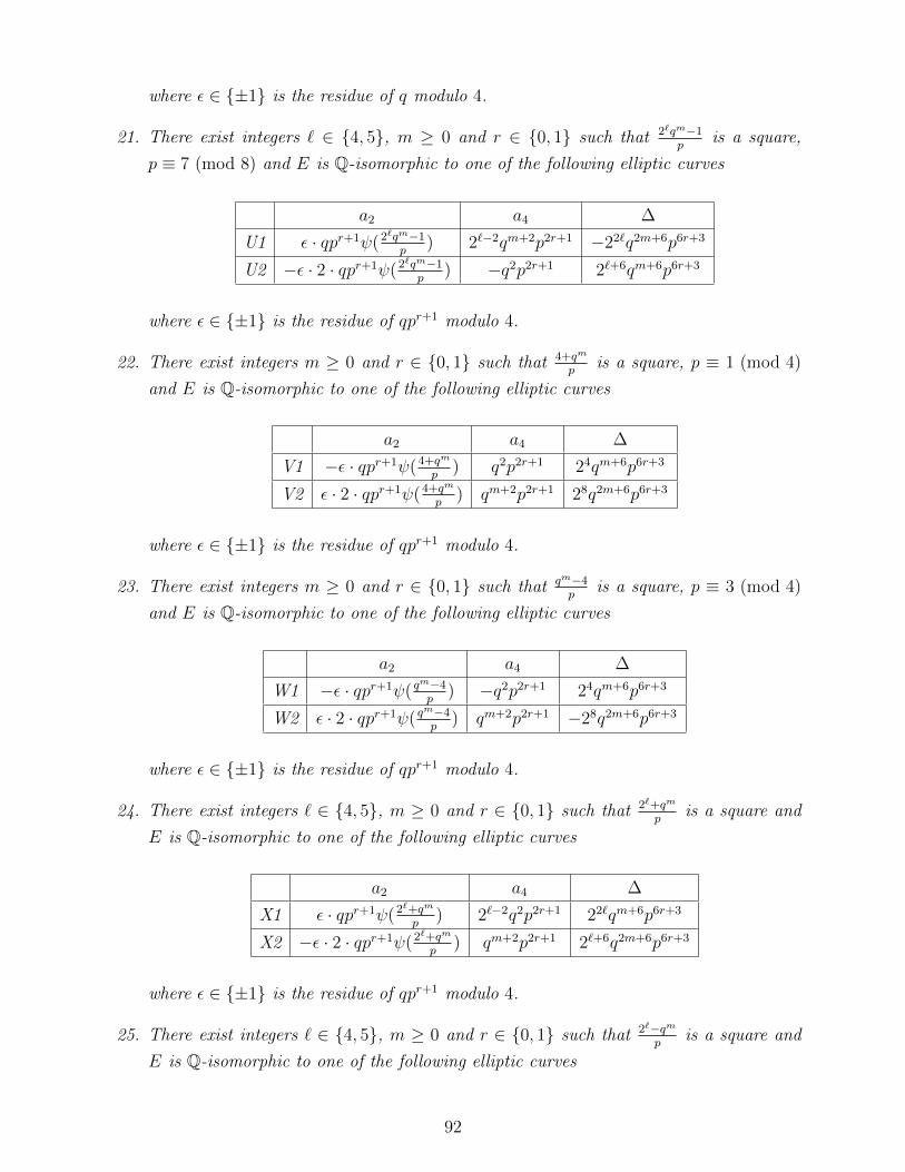
where ε ∈ ±1 is the residue of q modulo 4.
21. There exist integers ` ∈ 4, 5, m ≥ 0 and r ∈ 0, 1 such that 2`qm−1p
is a square,
p ≡ 7 (mod 8) and E is Q-isomorphic to one of the following elliptic curves
a2 a4 ∆
U1 ε · qpr+1ψ(2`qm−1p
) 2`−2qm+2p2r+1 −22`q2m+6p6r+3
U2 −ε · 2 · qpr+1ψ(2`qm−1p
) −q2p2r+1 2`+6qm+6p6r+3
where ε ∈ ±1 is the residue of qpr+1 modulo 4.
22. There exist integers m ≥ 0 and r ∈ 0, 1 such that 4+qm
pis a square, p ≡ 1 (mod 4)
and E is Q-isomorphic to one of the following elliptic curves
a2 a4 ∆
V1 −ε · qpr+1ψ(4+qm
p) q2p2r+1 24qm+6p6r+3
V2 ε · 2 · qpr+1ψ(4+qm
p) qm+2p2r+1 28q2m+6p6r+3
where ε ∈ ±1 is the residue of qpr+1 modulo 4.
23. There exist integers m ≥ 0 and r ∈ 0, 1 such that qm−4p
is a square, p ≡ 3 (mod 4)
and E is Q-isomorphic to one of the following elliptic curves
a2 a4 ∆
W1 −ε · qpr+1ψ( qm−4p
) −q2p2r+1 24qm+6p6r+3
W2 ε · 2 · qpr+1ψ( qm−4p
) qm+2p2r+1 −28q2m+6p6r+3
where ε ∈ ±1 is the residue of qpr+1 modulo 4.
24. There exist integers ` ∈ 4, 5, m ≥ 0 and r ∈ 0, 1 such that 2`+qm
pis a square and
E is Q-isomorphic to one of the following elliptic curves
a2 a4 ∆
X1 ε · qpr+1ψ(2`+qm
p) 2`−2q2p2r+1 22`qm+6p6r+3
X2 −ε · 2 · qpr+1ψ(2`+qm
p) qm+2p2r+1 2`+6q2m+6p6r+3
where ε ∈ ±1 is the residue of qpr+1 modulo 4.
25. There exist integers ` ∈ 4, 5, m ≥ 0 and r ∈ 0, 1 such that 2`−qmp
is a square and
E is Q-isomorphic to one of the following elliptic curves
92

a2 a4 ∆
Y1 ε · qpr+1ψ(2`−qmp
) 2`−2q2p2r+1 −22`qm+6p6r+3
Y2 −ε · 2 · qpr+1ψ(2`−qmp
) −qm+2p2r+1 2`+6q2m+6p6r+3
where ε ∈ ±1 is the residue of qpr+1 modulo 4.
26. There exist integers ` ∈ 4, 5, m ≥ 0 and r ∈ 0, 1 such that qm−2`
pis a square and
E is Q-isomorphic to one of the following elliptic curves
a2 a4 ∆
Z1 ε · qpr+1ψ( qm−2`
p) −2`−2q2p2r+1 22`qm+6p6r+3
Z2 −ε · 2 · qpr+1ψ( qm−2`
p) qm+2p2r+1 −2`+6q2m+6p6r+3
where ε ∈ ±1 is the residue of qpr+1 modulo 4.
27. There exist integers n ≥ 0 and s ∈ 0, 1 such that 4pn+1q
is a square, q ≡ 5 (mod 8),
pn ≡ 1 (mod 4) and E is Q-isomorphic to one of the following elliptic curves
a2 a4 ∆
AA1 −ε · qs+1pψ(4pn+1q
) q2s+1pn+2 24q6s+3p2n+6
AA2 ε · 2 · qs+1pψ(4pn+1q
) q2s+1p2 28q6s+3pn+6
where ε ∈ ±1 is the residue of p modulo 4.
28. There exist integers n ≥ 0 and s ∈ 0, 1 such that 4pn−1q
is a square, q ≡ 3 (mod 8),
pn ≡ 3 (mod 4) and E is Q-isomorphic to one of the following elliptic curves 2
a2 a4 ∆
AB1 −ε · qs+1pψ(4pn−1q
) q2s+1pn+2 −24q6s+3p2n+6
AB2 ε · 2 · qs+1pψ(4pn−1q
) −q2s+1p2 28q6s+3pn+6
where ε ∈ ±1 is the residue of qs+1p modulo 4.
29. There exist integers ` ∈ 4, 5, n ≥ 0 and s ∈ 0, 1 such that 2`pn+1q
is a square,
q ≡ 1 (mod 8) and E is Q-isomorphic to one of the following elliptic curves
a2 a4 ∆
AC1 ε · qs+1pψ(2`pn+1q
) 2`−2q2s+1pn+2 22`q6s+3p2n+6
AC2 −ε · 2 · qs+1pψ(2`pn+1q
) q2s+1p2 2`+6q6s+3pn+6
2Typo in [Mul06, p. 116] the two a2 values there are reversed. Also there are two Z curves.
93

where ε ∈ ±1 is the residue of p modulo 4.
30. There exist integers ` ∈ 4, 5, n ≥ 0 and s ∈ 0, 1 such that 2`pn−1q
is a square,
q ≡ 7 (mod 8) and E is Q-isomorphic to one of the following elliptic curves
a2 a4 ∆
AD1 ε · qs+1pψ(2`pn−1q
) 2`−2q2s+1pn+2 −22`q6s+3p2n+6
AD2 −ε · 2 · qs+1pψ(2`pn−1q
) −q2s+1p2 2`+6q6s+3pn+6
where ε ∈ ±1 is the residue of qs+1p modulo 4.
31. There exist integers n ≥ 0 and s ∈ 0, 1 such that 4+pn
qis a square, q ≡ 1 (mod 4)
and E is Q-isomorphic to one of the following elliptic curves
a2 a4 ∆
AE1 −ε · qs+1pψ(4+pn
q) q2s+1p2 24q6s+3pn+6
AE2 ε · 2 · qs+1pψ(4+pn
q) q2s+1pn+2 28q6s+3p2n+6
where ε ∈ ±1 is the residue of qs+1p modulo 4.
32. There exist integers n ≥ 0 and s ∈ 0, 1 such that pn−4q
is a square, q ≡ 3 (mod 4)
and E is Q-isomorphic to one of the following elliptic curve
a2 a4 ∆
AF1 −ε · qs+1pψ(pn−4q
) −q2s+1p2 24q6s+3pn+6
AF2 ε · 2 · qs+1pψ(pn−4q
) q2s+1pn+2 −28q6s+3p2n+6
where ε ∈ ±1 is the residue of qs+1p modulo 4.
33. There exist integers ` ∈ 4, 5, n ≥ 0 and s ∈ 0, 1 such that 2`+pn
qis a square and E
is Q-isomorphic to one of the following elliptic curves
a2 a4 ∆
AG1 ε · qs+1pψ(2`+pn
q) 2`−2q2s+1p2 22`q6s+3pn+6
AG2 −ε · 2 · qs+1pψ(2`+pn
q) q2s+1pn+2 2`+6q6s+3p2n+6
where ε ∈ ±1 is the residue of qs+1p modulo 4.
34. There exist integers ` ∈ 4, 5, n ≥ 0 and s ∈ 0, 1 such that 2`−pnq
is a square and E
is Q-isomorphic to one of the following elliptic curve
94

a2 a4 ∆
AH1 ε · qs+1pψ(2`−pnq
) 2`−2q2s+1p2 −22`q6s+3pn+6
AH2 −ε · 2 · qs+1pψ(2`−pnq
) −q2s+1pn+2 2`+6q6s+3p2n+6
where ε ∈ ±1 is the residue of qs+1p modulo 4.
35. There exist integers ` ∈ 4, 5, n ≥ 0 and s ∈ 0, 1 such that pn−2`
qis a square and E
is Q-isomorphic to one of the following elliptic curve
a2 a4 ∆
AI1 ε · qs+1pψ(pn−2`
q) −2`−2q2s+1p2 22`q6s+3pn+6
AI2 −ε · 2 · qs+1pψ(pn−2`
q) q2s+1pn+2 −2`+6q6s+3p2n+6
where ε ∈ ±1 is the residue of qs+1p modulo 4.
36. We have ` = 5, p, q ∈ 3, 11 distinct, r, s ∈ 0, 1 and E is Q-isomorphic to one of
the following elliptic curve
a2 a4 ∆
AJ1 ε · qs+1pr+1ψ(25+1qp
) 23q2s+1p2r+1 210q6s+3p6r+3
AJ2 −ε · 2 · qs+1pr+1ψ(25+1qp
) q2s+1p2r+1 211q6s+3p6r+3
where ε ∈ ±1 is the residue of qs+1pr+1 modulo 4.
37. We have ` = 4, p, q ∈ 3, 5 distinct, r, s ∈ 0, 1 and E is Q-isomorphic to one of the
following elliptic curve
a2 a4 ∆
AK1 ε · qs+1pr+1ψ(24−1qp
) 4q2s+1p2r+1 −28q6s+3p6r+3
AK2 −ε · 2 · qs+1pr+1ψ(24−1qp
) −q2s+1p2r+1 210q6s+3p6r+3
where ε ∈ ±1 is the residue of qs+1pr+1 modulo 4.
Theorem 2.2.14. The elliptic curves E defined over Q of conductor 24q2p2 and having at
least one rational point of order 2 are the ones such that one of the following conditions is
satisfied:
1. There exist integers ` ≥ 4, m ≥ 0 and n ≥ 0 such that 2`qmpn + 1 is a square and E is
Q-isomorphic to one of the following elliptic curves
95

a2 a4 ∆
A1 −ε · qpψ(2`qmpn + 1) 2`−2qm+2pn+2 22`q2m+6p2n+6
A2 ε · 2 · qpψ(2`qmpn + 1) q2p2 2`+6qm+6pn+6
where ε ∈ ±1 is the residue of qp modulo 4.
2. There exist integers m ≥ 0 and n ≥ 0 such that 4qm + pn is a square, qm ≡ 1 (mod 4),
n even or p ≡ 1 (mod 4), and E is Q-isomorphic to one of the following elliptic curves
a2 a4 ∆
B1 ε · qpψ(4qm + pn) qm+2p2 24q2m+6pn+6
B2 −ε · 2 · qpψ(4qm + pn) q2pn+2 28qm+6p2n+6
where ε ∈ ±1 is the residue of qm+1p modulo 4.
3. There exist integers m ≥ 0 and n ≥ 0 such that 4qm − pn is a square, qm ≡ 1 (mod 4),
n odd and p ≡ 3 (mod 8), and E is Q-isomorphic to one of the following elliptic curves
a2 a4 ∆
C1 ε · qpψ(4qm − pn) qm+2p2 −24q2m+6pn+6
C2 −ε · 2 · qpψ(4qm − pn) −q2pn+2 28qm+6p2n+6
where ε ∈ ±1 is the residue of qm+1p modulo 4.
4. There exist integers m ≥ 0 and n ≥ 0 such that pn−4qm is a square, qm ≡ −1 (mod 4),
n even or p ≡ 1 (mod 4), and E is Q-isomorphic to one of the following elliptic curves
a2 a4 ∆
D1 ε · qpψ(pn − 4qm) −qm+2p2 24q2m+6pn+6
D2 −ε · 2 · qpψ(pn − 4qm) q2pn+2 −28qm+6p2n+6
where ε ∈ ±1 is the residue of qm+1p modulo 4.
5. There exist integers ` ≥ 4, m ≥ 0 and n ≥ 0 such that 2`qm + pn is a square and E is
Q-isomorphic to one of the following elliptic curves
a2 a4 ∆
E1 −ε · qpψ(2`qm + pn) 2`−2qm+2p2 22`q2m+6pn+6
E2 ε · 2 · qpψ(2`qm + pn) q2pn+2 2`+6qm+6p2n+6
where ε ∈ ±1 is the residue of qp modulo 4.
96

6. There exist integers ` ≥ 4, m ≥ 0 and n ≥ 0 such that 2`qm − pn is a square, p ≡7 (mod 8), n odd and E is Q-isomorphic to one of the following elliptic curves
a2 a4 ∆
F1 −ε · qpψ(2`qm − pn) 2`−2qm+2p2 −22`q2m+6pn+6
F2 ε · 2 · qpψ(2`qm − pn) −q2pn+2 2`+6qm+6p2n+6
where ε ∈ ±1 is the residue of qp modulo 4.
7. There exist integers ` ≥ 4, m ≥ 0 and n ≥ 0 such that pn − 2`qm is a square and E is
Q-isomorphic to one of the following elliptic curves
a2 a4 ∆
G1 −ε · qpψ(pn − 2`qm) −2`−2qm+2p2 22`q2m+6pn+6
G2 ε · 2 · qpψ(pn − 2`qm) q2pn+2 −2`+6qm+6p2n+6
where ε ∈ ±1 is the residue of qp modulo 4.
8. There exist integers m ≥ 0 and n ≥ 0 such that 4pn + qm is a square, q ≡ 5 (mod 8)
and E is Q-isomorphic to one of the following elliptic curves
a2 a4 ∆
H1 ε · qpψ(4pn + qm) q2pn+2 24qm+6p2n+6
H2 −ε · 2 · qpψ(4pn + qm) qm+2p2 28q2m+6pn+6
where ε ∈ ±1 is the residue of pn+1 modulo 4.
9. There exist integers m ≥ 0 and n ≥ 0 such that 4pn − qm is a square, q ≡ 3 (mod 8),
and E is Q-isomorphic to one of the following elliptic curves
a2 a4 ∆
I1 ε · qpψ(4pn − qm) q2pn+2 −24qm+6p2n+6
I2 −ε · 2 · qpψ(4pn − qm) −qm+2p2 28q2m+6pn+6
where ε ∈ ±1 is the residue of qpn+1 modulo 4.
10. There exist integers m ≥ 0 and n ≥ 0 such that qm − 4pn is a square, q ≡ 5 (mod 8),
and E is Q-isomorphic to one of the following elliptic curves
a2 a4 ∆
J1 ε · qpψ(qm − 4pn) −q2pn+2 24qm+6p2n+6
J2 −ε · 2 · qpψ(qm − 4pn) qm+2p2 −28q2m+6pn+6
97

where ε ∈ ±1 is the residue of −pn+1 modulo 4.
11. There exist integers ` ≥ 4, m ≥ 0 and n ≥ 0 such that 2`pn + qm is a square and E is
Q-isomorphic to one of the following elliptic curves
a2 a4 ∆
K1 −ε · qpψ(2`pn + qm) 2`−2q2pn+2 22`qm+6p2n+6
K2 ε · 2 · qpψ(2`pn + qm) qm+2p2 2`+6q2m+6pn+6
where ε ∈ ±1 is the residue of qp modulo 4.
12. There exist integers ` ≥ 4, m ≥ 0 and n ≥ 0 such that 2`pn − qm is a square, q ≡7 (mod 8), m odd and E is Q-isomorphic to one of the following elliptic curves
a2 a4 ∆
L1 −ε · qpψ(2`pn − qm) 2`−2q2pn+2 −22`qm+6p2n+6
L2 ε · 2 · qpψ(2`pn − qm) −qm+2p2 2`+6q2m+6pn+6
where ε ∈ ±1 is the residue of qp modulo 4.
13. There exist integers ` ≥ 4, m ≥ 0 and n ≥ 0 such that qm − 2`pn is a square and E is
Q-isomorphic to one of the following elliptic curves
a2 a4 ∆
M1 −ε · qpψ(qm − 2`pn) −2`−2q2pn+2 22`qm+6p2n+6
M2 ε · 2 · qpψ(qm − 2`pn) qm+2p2 −2`+6q2m+6pn+6
where ε ∈ ±1 is the residue of qp modulo 4.
14. There exist integers m ≥ 0 and n ≥ 0 such that 4 + qmpn is a square and E is Q-
isomorphic to one of the following elliptic curves
a2 a4 ∆
N1 ε · qpψ(4 + qmpn) q2p2 24qm+6pn+6
N2 −ε · 2 · qpψ(4 + qmpn) qm+2pn+2 28q2m+6p2n+6
where ε ∈ ±1 is the residue of qp modulo 4.
15. There exist integers m ≥ 0 and n ≥ 0 such that qmpn − 4 is a square, p ≡ 1 (mod 4) if
n ≥ 1, q ≡ 1 (mod 4) if m ≥ 1, and E is Q-isomorphic to one of the following elliptic
curves
98

a2 a4 ∆
O1 −εqpψ(qmpn − 4) −q2p2 24qm+6pn+6
O2 ε · 2 · qpψ(qmpn − 4) qm+2pn+2 −28q2m+6p2n+6
where ε ∈ ±1 is the residue of qp modulo 4.
16. There exist integers ` ≥ 4, m ≥ 0 and n ≥ 0 such that 2` + qmpn is a square and E is
Q-isomorphic to one of the following elliptic curves
a2 a4 ∆
P1 −ε · qpψ(2` + qmpn) 2`−2q2p2 22`qm+6pn+6
P2 ε · 2 · qpψ(2` + qmpn) qm+2pn+2 2`+6q2m+6p2n+6
where ε ∈ ±1 is the residue of qp modulo 4.
17. There exist integers ` ≥ 4, m ≥ 0 and n ≥ 0 such that 2` − qmpn is a square and E is
Q-isomorphic to one of the following elliptic curves
a2 a4 ∆
Q1 −ε · qpψ(2` − qmpn) 2`−2q2p2 −22`qm+6pn+6
Q2 ε · 2 · qpψ(2` − qmpn) −qm+2pn+2 2`+6q2m+6p2n+6
where ε ∈ ±1 is the residue of qp modulo 4.
18. There exist integers ` ≥ 4, m ≥ 0 and n ≥ 0 such that qmpn − 2` is a square and E is
Q-isomorphic to one of the following elliptic curves
a2 a4 ∆
R1 −ε · qpψ(qmpn − 2`) −2`−2q2p2 22`qm+6pn+6
R2 ε · 2 · qpψ(qmpn − 2`) qm+2pn+2 −2`+6q2m+6p2n+6
where ε ∈ ±1 is the residue of qp modulo 4.
19. There exist integers m ≥ 0 and r ∈ 0, 1 such that 4qm+1p
is a square, p ≡ 5 (mod 8)
and E is Q-isomorphic to one of the following elliptic curves 3
a2 a4 ∆
S1 ε · qpr+1ψ(4qm+1p
) qm+2p2r+1 24q2m+6p6r+3
S2 −ε · 2 · qpr+1ψ(4qm+1p
) q2p2r+1 28qm+6p6r+3
3Typo in [Mul06, p. 120], the 2m should be removed.
99

where ε ∈ ±1 is the residue of qm+1pr modulo 4.
20. There exist integers m ≥ 0 and r ∈ 0, 1 such that 4qm−1p
is a square, p ≡ 3 (mod 8)
and E is Q-isomorphic to one of the following elliptic curves 4
a2 a4 ∆
T1 ε · qpr+1ψ(4qm−1p
) qm+2p2r+1 −24q2m+6p6r+3
T2 −ε · 2 · qpr+1ψ(4qm−1p
) −q2p2r+1 28qm+6p6r+3
where ε ∈ ±1 is the residue of qm+1pr modulo 4.
21. There exist integers ` ≥ 4, m ≥ 0 and r ∈ 0, 1 such that 2`qm+1p
is a square, p ≡1 (mod 8) and E is Q-isomorphic to one of the following elliptic curves 5
a2 a4 ∆
U1 −ε · qpr+1ψ(2`qm+1p
) 2`−2qm+2p2r+1 22`q2m+6p6r+3
U2 ε · 2 · qpr+1ψ(2`qm+1p
) q2p2r+1 2`+6qm+6p6r+3
where ε ∈ ±1 is the residue of q modulo 4.
22. There exist integers ` ≥ 4, m ≥ 0 and r ∈ 0, 1 such that 2`qm−1p
is a square, p ≡7 (mod 8) and E is Q-isomorphic to one of the following elliptic curves 6
a2 a4 ∆
V1 −ε · qpr+1ψ(2`qm−1p
) 2`−2qm+2p2r+1 −22`q2m+6p6r+3
V2 ε · 2 · qpr+1ψ(2`qm−1p
) −q2p2r+1 2`+6qm+6p6r+3
where ε ∈ ±1 is the residue of qpr+1 modulo 4.
23. There exist integers m ≥ 0 and r ∈ 0, 1 such that 4+qm
pis a square and E is Q-
isomorphic to one of the following elliptic curves
a2 a4 ∆
W1 ε · qpr+1ψ(4+qm
p) q2p2r+1 24qm+6p6r+3
W2 −ε · 2 · qpr+1ψ(4+qm
p) qm+2p2r+1 28q2m+6p6r+3
where ε ∈ ±1 is the residue of qpr modulo 4.
4Typo in [Mul06, p. 121], the 2m should be removed.5Typo in [Mul06, p. 121], the 2m should be 2m−2.6Typo in [Mul06, p. 121], the 2m should be 2m−2.
100

24. There exist integers m ≥ 0 and r ∈ 0, 1 such that qm−4p
is a square and E is Q-
isomorphic to one of the following elliptic curves
a2 a4 ∆
X1 ε · qpr+1ψ( qm−4p
) −q2p2r+1 24qm+6p6r+3
X2 −ε · 2 · qpr+1ψ( qm−4p
) qm+2p2r+1 −28q2m+6p6r+3
where ε ∈ ±1 is the residue of −qpr modulo 4.
25. There exist integers ` ≥ 4, m ≥ 0 and r ∈ 0, 1 such that 2`+qm
pis a square and E is
Q-isomorphic to one of the following elliptic curves
a2 a4 ∆
Y1 −ε · qpr+1ψ(2`+qm
p) 2`−2q2p2r+1 22`qm+6p6r+3
Y2 ε · 2 · qpr+1ψ(2`+qm
p) qm+2p2r+1 2`+6q2m+6p6r+3
where ε ∈ ±1 is the residue of qpr+1 modulo 4.
26. There exist integers ` ≥ 4, m ≥ 0 and r ∈ 0, 1 such that 2`−qmp
is a square and E is
Q-isomorphic to one of the following elliptic curves
a2 a4 ∆
Z1 −ε · qpr+1ψ(2`−qmp
) 2`−2q2p2r+1 −22`qm+6p6r+3
Z2 ε · 2 · qpr+1ψ(2`−qmp
) −qm+2p2r+1 2`+6q2m+6p6r+3
where ε ∈ ±1 is the residue of qpr+1 modulo 4.
27. There exist integers ` ≥ 4, m ≥ 0 and r ∈ 0, 1 such that qm−2`
pis a square and E is
Q-isomorphic to one of the following elliptic curves
a2 a4 ∆
AA1 −ε · qpr+1ψ( qm−2`
p) −2`−2q2p2r+1 22`qm+6p6r+3
AA2 ε · 2 · qpr+1ψ( qm−2`
p) qm+2p2r+1 −2`+6q2m+6p6r+3
where ε ∈ ±1 is the residue of qpr+1 modulo 4.
28. There exist integers n ≥ 0 and s ∈ 0, 1 such that 4pn+1q
is a square, q ≡ 5 (mod 8)
and E is Q-isomorphic to one of the following elliptic curves
a2 a4 ∆
AB1 ε · qs+1pψ(4pn+1q
) q2s+1pn+2 24q6s+3p2n+6
AB2 −ε · 2 · qs+1pψ(4pn+1q
) q2s+1p2 28q6s+3pn+6
101

where ε ∈ ±1 is the residue of qspn+1 modulo 4.
29. There exist integers n ≥ 0 and s ∈ 0, 1 such that 4pn−1q
is a square, q ≡ 3 (mod 8)
and E is Q-isomorphic to one of the following elliptic curves
a2 a4 ∆
AC1 ε · qs+1pψ(4pn−1q
) q2s+1pn+2 −24q6s+3p2n+6
AC2 −ε · 2 · qs+1pψ(4pn−1q
) −q2s+1p2 28q6s+3pn+6
where ε ∈ ±1 is the residue of qspn+1 modulo 4.
30. There exist integers ` ≥ 4, n ≥ 0 and s ∈ 0, 1 such that 2`pn+1q
is a square, q ≡1 (mod 8) and E is Q-isomorphic to one of the following elliptic curves
a2 a4 ∆
AD1 −ε · qs+1pψ(2`pn+1q
) 2`−2q2s+1pn+2 22`q6s+3p2n+6
AD2 ε · 2 · qs+1pψ(2`pn+1q
) q2s+1p2 2`+6q6s+3pn+6
where ε ∈ ±1 is the residue of p modulo 4.
31. There exist integers ` ≥ 4, n ≥ 0 and s ∈ 0, 1 such that 2`pn−1q
is a square, q ≡7 (mod 8) and E is Q-isomorphic to one of the following elliptic curves
a2 a4 ∆
AE1 −ε · qs+1pψ(2`pn−1q
) 2`−2q2s+1pn+2 −22`q6s+3p2n+6
AE2 ε · 2 · qs+1pψ(2`pn−1q
) −q2s+1p2 2`+6q6s+3pn+6
where ε ∈ ±1 is the residue of qs+1p modulo 4.
32. There exist integers n ≥ 0 and s ∈ 0, 1 such that 4+pn
qis a square and E is Q-
isomorphic to one of the following elliptic curves
a2 a4 ∆
AF1 ε · qs+1pψ(4+pn
q) q2s+1p2 24q6s+3pn+6
AF2 −ε · 2 · qs+1pψ(4+pn
q) q2s+1pn+2 28q6s+3p2n+6
where ε ∈ ±1 is the residue of qsp modulo 4.
33. There exist integers n ≥ 0 and s ∈ 0, 1 such that pn−4q
is a square and E is Q-
isomorphic to one of the following elliptic curve
102

a2 a4 ∆
AG1 ε · qs+1pψ(pn−4q
) −q2s+1p2 24q6s+3pn+6
AG2 −ε · 2 · qs+1pψ(pn−4q
) q2s+1pn+2 −28q6s+3p2n+6
where ε ∈ ±1 is the residue of −qsp modulo 4.
34. There exist integers ` ≥ 4, n ≥ 0 and s ∈ 0, 1 such that 2`+pn
qis a square and E is
Q-isomorphic to one of the following elliptic curves
a2 a4 ∆
AH1 −ε · qs+1pψ(2`+pn
q) 2`−2q2s+1p2 22`q6s+3pn+6
AH2 ε · 2 · qs+1pψ(2`+pn
q) q2s+1pn+2 2`+6q6s+3p2n+6
where ε ∈ ±1 is the residue of qs+1p modulo 4.
35. There exist integers ` ≥ 4, n ≥ 0 and s ∈ 0, 1 such that 2`−pnq
is a square and E is
Q-isomorphic to one of the following elliptic curve
a2 a4 ∆
AI1 −ε · qs+1pψ(2`−pnq
) 2`−2q2s+1p2 −22`q6s+3pn+6
AI2 ε · 2 · qs+1pψ(2`−pnq
) −q2s+1pn+2 2`+6q6s+3p2n+6
where ε ∈ ±1 is the residue of qs+1p modulo 4.
36. There exist integers ` ≥ 4, n ≥ 0 and s ∈ 0, 1 such that pn−2`
qis a square and E is
Q-isomorphic to one of the following elliptic curve
a2 a4 ∆
AJ1 −ε · qs+1pψ(pn−2`
q) −2`−2q2s+1p2 22`q6s+3pn+6
AJ2 ε · 2 · qs+1pψ(pn−2`
q) q2s+1pn+2 −2`+6q6s+3p2n+6
where ε ∈ ±1 is the residue of qs+1p modulo 4.
37. There exist integers ` ≥ 4 and r, s ∈ 0, 1 such that 2`+1qp
is a square and E is Q-
isomorphic to one of the following elliptic curve
a2 a4 ∆
AK1 −ε · qs+1pr+1ψ(2`+1qp
) 2`−2q2s+1p2r+1 22`q6s+3p6r+3
AK2 ε · 2 · qs+1pr+1ψ(2`+1qp
) q2s+1p2r+1 2`+6q6s+3p6r+3
where ε ∈ ±1 is the residue of qs+1pr+1 modulo 4.
103
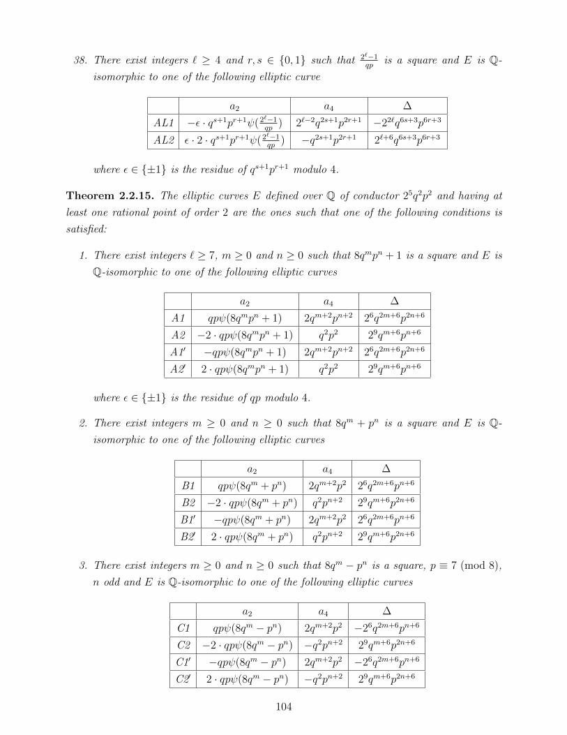
38. There exist integers ` ≥ 4 and r, s ∈ 0, 1 such that 2`−1qp
is a square and E is Q-
isomorphic to one of the following elliptic curve
a2 a4 ∆
AL1 −ε · qs+1pr+1ψ(2`−1qp
) 2`−2q2s+1p2r+1 −22`q6s+3p6r+3
AL2 ε · 2 · qs+1pr+1ψ(2`−1qp
) −q2s+1p2r+1 2`+6q6s+3p6r+3
where ε ∈ ±1 is the residue of qs+1pr+1 modulo 4.
Theorem 2.2.15. The elliptic curves E defined over Q of conductor 25q2p2 and having at
least one rational point of order 2 are the ones such that one of the following conditions is
satisfied:
1. There exist integers ` ≥ 7, m ≥ 0 and n ≥ 0 such that 8qmpn + 1 is a square and E is
Q-isomorphic to one of the following elliptic curves
a2 a4 ∆
A1 qpψ(8qmpn + 1) 2qm+2pn+2 26q2m+6p2n+6
A2 −2 · qpψ(8qmpn + 1) q2p2 29qm+6pn+6
A1′ −qpψ(8qmpn + 1) 2qm+2pn+2 26q2m+6p2n+6
A2′ 2 · qpψ(8qmpn + 1) q2p2 29qm+6pn+6
where ε ∈ ±1 is the residue of qp modulo 4.
2. There exist integers m ≥ 0 and n ≥ 0 such that 8qm + pn is a square and E is Q-
isomorphic to one of the following elliptic curves
a2 a4 ∆
B1 qpψ(8qm + pn) 2qm+2p2 26q2m+6pn+6
B2 −2 · qpψ(8qm + pn) q2pn+2 29qm+6p2n+6
B1′ −qpψ(8qm + pn) 2qm+2p2 26q2m+6pn+6
B2′ 2 · qpψ(8qm + pn) q2pn+2 29qm+6p2n+6
3. There exist integers m ≥ 0 and n ≥ 0 such that 8qm − pn is a square, p ≡ 7 (mod 8),
n odd and E is Q-isomorphic to one of the following elliptic curves
a2 a4 ∆
C1 qpψ(8qm − pn) 2qm+2p2 −26q2m+6pn+6
C2 −2 · qpψ(8qm − pn) −q2pn+2 29qm+6p2n+6
C1′ −qpψ(8qm − pn) 2qm+2p2 −26q2m+6pn+6
C2′ 2 · qpψ(8qm − pn) −q2pn+2 29qm+6p2n+6
104
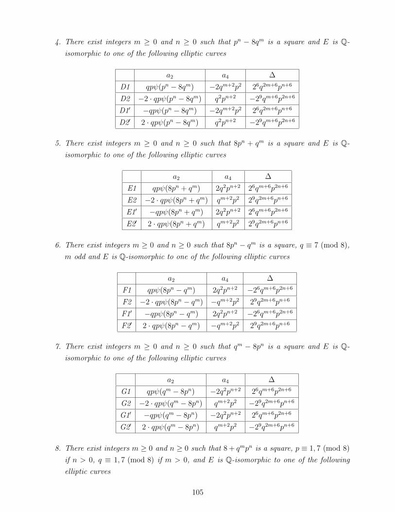
4. There exist integers m ≥ 0 and n ≥ 0 such that pn − 8qm is a square and E is Q-
isomorphic to one of the following elliptic curves
a2 a4 ∆
D1 qpψ(pn − 8qm) −2qm+2p2 26q2m+6pn+6
D2 −2 · qpψ(pn − 8qm) q2pn+2 −29qm+6p2n+6
D1′ −qpψ(pn − 8qm) −2qm+2p2 26q2m+6pn+6
D2′ 2 · qpψ(pn − 8qm) q2pn+2 −29qm+6p2n+6
5. There exist integers m ≥ 0 and n ≥ 0 such that 8pn + qm is a square and E is Q-
isomorphic to one of the following elliptic curves
a2 a4 ∆
E1 qpψ(8pn + qm) 2q2pn+2 26qm+6p2n+6
E2 −2 · qpψ(8pn + qm) qm+2p2 29q2m+6pn+6
E1′ −qpψ(8pn + qm) 2q2pn+2 26qm+6p2n+6
E2′ 2 · qpψ(8pn + qm) qm+2p2 29q2m+6pn+6
6. There exist integers m ≥ 0 and n ≥ 0 such that 8pn − qm is a square, q ≡ 7 (mod 8),
m odd and E is Q-isomorphic to one of the following elliptic curves
a2 a4 ∆
F1 qpψ(8pn − qm) 2q2pn+2 −26qm+6p2n+6
F2 −2 · qpψ(8pn − qm) −qm+2p2 29q2m+6pn+6
F1′ −qpψ(8pn − qm) 2q2pn+2 −26qm+6p2n+6
F2′ 2 · qpψ(8pn − qm) −qm+2p2 29q2m+6pn+6
7. There exist integers m ≥ 0 and n ≥ 0 such that qm − 8pn is a square and E is Q-
isomorphic to one of the following elliptic curves
a2 a4 ∆
G1 qpψ(qm − 8pn) −2q2pn+2 26qm+6p2n+6
G2 −2 · qpψ(qm − 8pn) qm+2p2 −29q2m+6pn+6
G1′ −qpψ(qm − 8pn) −2q2pn+2 26qm+6p2n+6
G2′ 2 · qpψ(qm − 8pn) qm+2p2 −29q2m+6pn+6
8. There exist integers m ≥ 0 and n ≥ 0 such that 8 + qmpn is a square, p ≡ 1, 7 (mod 8)
if n > 0, q ≡ 1, 7 (mod 8) if m > 0, and E is Q-isomorphic to one of the following
elliptic curves
105

a2 a4 ∆
H1 qpψ(8 + qmpn) 2q2p2 26qm+6pn+6
H2 −2 · qpψ(8 + qmpn) qm+2pn+2 29q2m+6p2n+6
H1′ −qpψ(8 + qmpn) 2q2p2 26qm+6pn+6
H2′ 2 · qpψ(8 + qmpn) qm+2pn+2 29q2m+6p2n+6
9. There exist integers m ≥ 0 and n ≥ 0 such that qmpn − 8 is a square, p ≡ 1, 3 (mod 8)
if n > 0, q ≡ 1, 3 (mod 8) if m > 0, and E is Q-isomorphic to one of the following
elliptic curves
a2 a4 ∆
I1 qpψ(qmpn − 8) −2q2p2 26qm+6pn+6
I2 −2 · qpψ(qmpn − 8) qm+2pn+2 −29q2m+6p2n+6
I1′ −qpψ(qmpn − 8) −2q2p2 26qm+6pn+6
I2′ 2 · qpψ(qmpn − 8) qm+2pn+2 −29q2m+6p2n+6
10. There exist integers m ≥ 0 and n ≥ 0 such that qmpn + 1 is a square and E is Q-
isomorphic to one of the following elliptic curves
a2 a4 ∆
J1 2qpψ(qmpn + 1) qm+2pn+2 26q2m+6p2n+6
J2 −4 · qpψ(qmpn + 1) 4q2p2 212qm+6pn+6
J1′ −2qpψ(qmpn + 1) qm+2pn+2 26q2m+6p2n+6
J2′ 4 · qpψ(qmpn + 1) 4q2p2 212qm+6pn+6
11. There exist integers m ≥ 0 and n ≥ 0 such that qmpn − 1 is a square, p ≡ 1 (mod 4) if
n > 0, q ≡ 1 (mod 4) if m > 0, and E is Q-isomorphic to one of the following elliptic
curves
a2 a4 ∆
K1 2qpψ(qmpn − 1) q2p2 26q2m+6p2n+6
K2 −4 · qpψ(qmpn − 1) 4qm+2pn+2 212qm+6pn+6
K1′ −2qpψ(qmpn − 1) q2p2 26q2m+6p2n+6
K2′ 4 · qpψ(qmpn − 1) 4qm+2pn+2 212qm+6pn+6
12. There exist integers m ≥ 0 and n ≥ 0 such that qm + pn is a square and E is Q-
isomorphic to one of the following elliptic curves
(a) m is even or q ≡ 1 (mod 4);
106

a2 a4 ∆
L1 2qpψ(qm + pn) q2pn+2 26qm+6p2n+6
L2 −4 · qpψ(qm + pn) 4qm+2p2 212q2m+6pn+6
L1′ −2qpψ(qm + pn) q2pn+2 26qm+6p2n+6
L2′ 4 · qpψ(qm + pn) 4qm+2p2 212q2m+6pn+6
(b) m is odd and q ≡ 3 (mod 4);
a2 a4 ∆
M1 2qpψ(qm + pn) qm+2p2 26q2m+6pn+6
M2 −4 · qpψ(qm + pn) 4q2pn+2 212qm+6p2n+6
M1′ −2qpψ(qm + pn) qm+2p2 26q2m+6pn+6
M2′ 4 · qpψ(qm + pn) 4q2pn+2 212qm+6p2n+6
13. There exist integers m ≥ 0 and n ≥ 0 such that qm − pn is a square and E is Q-
isomorphic to one of the following elliptic curves
(a) m is even or q ≡ 1 (mod 4);
a2 a4 ∆
N1 2qpψ(qm − pn) −q2pn+2 26qm+6p2n+6
N2 −4 · qpψ(qm − pn) 4qm+2 −212q2m+6pn+2
N1′ −2qpψ(qm − pn) −q2pn+2 26qm+6p2n+6
N2′ 4 · qpψ(qm − pn) 4qm+2 −212q2m+6pn+2
(b) m is odd and q ≡ 3 (mod 4);
a2 a4 ∆
O1 2qpψ(qm − pn) qm+2p2 −26q2m+6pn+6
O2 −4 · qpψ(qm − pn) −4q2pn+2 212qm+6p2n+6
O1′ −2qpψ(qm − pn) qm+2p2 −26q2m+6pn+6
O2′ 4 · qpψ(qm − pn) −4q2pn+2 212qm+6p2n+6
14. There exist integers m ≥ 0 and n ≥ 0 such that pn − qm is a square and E is Q-
isomorphic to one of the following elliptic curves
(a) m is even or q ≡ 1 (mod 4);
a2 a4 ∆
P1 2qpψ(pn − qm) −q2pn+2 26qm+6p2n+6
P2 −4 · qpψ(pn − qm) 4qm+2p2 −212q2m+6pn+6
P1′ −2qpψ(pn − qm) −q2pn+2 26qm+6p2n+6
P2′ 4 · qpψ(pn − qm) 4qm+2p2 −212q2m+6pn+6
107

(b) m is odd and q ≡ 3 (mod 4);
a2 a4 ∆
Q1 2qpψ(pn − qm) qm+2p2 −26q2m+6pn+6
Q2 −4 · qpψ(pn − qm) −4q2pn+2 212qm+6p2n+6
Q1′ −2qpψ(pn − qm) qm+2p2 −26q2m+6pn+6
Q2′ 4 · qpψ(pn − qm) −4q2pn+2 212qm+6p2n+6
15. There exist integers m ≥ 0 and r ∈ 0, 1 such that 8qm+1p
is a square, p ≡ 1 (mod 8)
and E is Q-isomorphic to one of the following elliptic curves
a2 a4 ∆
R1 qpr+1ψ(8qm+1p
) 2qm+2p2r+1 26q2m+6p6r+3
R2 −2 · qpr+1ψ(8qm+1p
) q2p2r+1 29qm+6p6r+3
R1′ −qpr+1ψ(8qm+1p
) 2qm+2p2r+1 26q2m+6p6r+3
R2′ 2 · qpr+1ψ(8qm+1p
) q2p2r+1 29qm+6p6r+3
16. There exist integers m ≥ 0 and r ∈ 0, 1 such that 8qm−1p
is a square, p ≡ 7 (mod 8)
and E is Q-isomorphic to one of the following elliptic curves
a2 a4 ∆
S1 qpr+1ψ(8qm−1p
) 2qm+2p2r+1 −26q2m+6p6r+3
S2 −2 · qpr+1ψ(8qm−1p
) −q2p2r+1 29qm+6p6r+3
S1′ −qpr+1ψ(8qm−1p
) 2qm+2p2r+1 −26q2m+6p6r+3
S2′ 2 · qpr+1ψ(8qm−1p
) −q2p2r+1 29qm+6p6r+3
17. There exist integers m ≥ 0 and r ∈ 0, 1 such that 8+qm
pis a square and E is Q-
isomorphic to one of the following elliptic curves
a2 a4 ∆
T1 qpr+1ψ(8+qm
p) 2q2p2r+1 26qm+6p6r+3
T2 −2 · qpr+1ψ(8+qm
p) qm+2p2r+1 29q2m+6p6r+3
T1′ −qpr+1ψ(8+qm
p) 2q2p2r+1 26qm+6p6r+3
T2′ 2 · qpr+1ψ(8+qm
p) qm+2p2r+1 29q2m+6p6r+3
18. There exist integers m ≥ 0 and r ∈ 0, 1 such that 8−qmp
is a square and E is Q-
isomorphic to one of the following elliptic curves
108

a2 a4 ∆
U1 qpr+1ψ(8−qmp
) 2q2p2r+1 −26qm+6p6r+3
U2 −2 · qpr+1ψ(8−qmp
) −qm+2p2r+1 29q2m+6p6r+3
U1′ −qpr+1ψ(8−qmp
) 2q2p2r+1 −26qm+6p6r+3
U2′ 2 · qpr+1ψ(8−qmp
) −qm+2p2r+1 29q2m+6p6r+3
19. There exist integers m ≥ 0 and r ∈ 0, 1 such that qm−8p
is a square and E is Q-
isomorphic to one of the following elliptic curves
a2 a4 ∆
V1 qpr+1ψ( qm−8p
) −2q2p2r+1 26qm+6p6r+3
V2 −2 · qpr+1ψ( qm−8p
) qm+2p2r+1 −29q2m+6p6r+3
V1′ −qpr+1ψ( qm−8p
) −2q2p2r+1 26qm+6p6r+3
V2′ 2 · qpr+1ψ( qm−8p
) qm+2p2r+1 −29q2m+6p6r+3
20. There exist integers n ≥ 0 and s ∈ 0, 1 such that 8pn+1q
is a square, q ≡ 1 (mod 8)
and E is Q-isomorphic to one of the following elliptic curves
a2 a4 ∆
W1 qs+1pψ(8pn+1q
) 2q2s+1pn+2 26q6s+3p2n+6
W2 −2 · qs+1pψ(8pn+1q
) q2s+1p2 29q6s+3pn+6
W1′ −qs+1pψ(8pn+1q
) 2q2s+1pn+2 26q6s+3p2n+6
W2′ 2 · qs+1pψ(8pn+1q
) q2s+1p2 29q6s+3pn+6
21. There exist integers n ≥ 0 and s ∈ 0, 1 such that 8pn−1q
is a square, q ≡ 7 (mod 8)
and E is Q-isomorphic to one of the following elliptic curves
a2 a4 ∆
X1 qs+1pψ(8pn−1q
) 2q2s+1pn+2 −26q6s+3p2n+6
X2 −2 · qs+1pψ(8pn−1q
) −q2s+1p2 29q6s+3pn+6
X1′ −qs+1pψ(8pn−1q
) 2q2s+1pn+2 −26q6s+3p2n+6
X2′ 2 · qs+1pψ(8pn−1q
) −q2s+1p2 29q6s+3pn+6
22. There exist integers n ≥ 0 and s ∈ 0, 1 such that 8+pn
qis a square and E is Q-
isomorphic to one of the following elliptic curves
a2 a4 ∆
Y1 qs+1pψ(8+pn
q) 2q2s+1p2 26q6s+3pn+6
Y2 −2 · qs+1pψ(8+pn
q) q2s+1pn+2 29q6s+3p2n+6
Y1′ −qs+1pψ(8+pn
q) 2q2s+1p2 26q6s+3pn+6
Y2′ 2 · qs+1pψ(8+pn
q) q2s+1pn+2 29q6s+3p2n+6
109

where ε ∈ ±1 is the residue of qs+1p modulo 4.
23. There exist integers n ≥ 0 and s ∈ 0, 1 such that 8−pnq
is a square and E is Q-
isomorphic to one of the following elliptic curve
a2 a4 ∆
Z1 qs+1pψ(8−pnq
) 2q2s+1p2 −26q6s+3pn+6
Z2 −2 · qs+1pψ(8−pnq
) −q2s+1pn+2 29q6s+3p2n+6
Z1′ −qs+1pψ(8−pnq
) 2q2s+1p2 −26q6s+3pn+6
Z2′ 2 · qs+1pψ(8−pnq
) −q2s+1pn+2 29q6s+3p2n+6
where ε ∈ ±1 is the residue of qs+1p modulo 4.
24. There exist integers n ≥ 0 and s ∈ 0, 1 such that pn−8q
is a square and E is Q-
isomorphic to one of the following elliptic curve
a2 a4 ∆
AA1 qs+1pψ(pn−8q
) −2q2s+1p2 26q6s+3pn+6
AA2 −2 · qs+1pψ(pn−8q
) q2s+1pn+2 −29q6s+3p2n+6
AA1′ −qs+1pψ(pn−8q
) −2q2s+1p2 26q6s+3pn+6
AA2′ 2 · qs+1pψ(pn−8q
) q2s+1pn+2 −29q6s+3p2n+6
where ε ∈ ±1 is the residue of qs+1p modulo 4.
25. There exist integers m ≥ 0 and r ∈ 0, 1 such that qm+1p
is a square, qm ≡ −1 (mod 4)
and E is Q-isomorphic to one of the following elliptic curves
(a) p ≡ 1 (mod 4);
a2 a4 ∆
AB1 2qpr+1ψ( qm+1p
) qm+2p2r+1 26q2m+6p6r+3
AB2 −4 · qpr+1ψ( qm+1p
) 4q2p2r+1 212qm+6p6r+3
AB1′ −2qpr+1ψ( qm+1p
) qm+2p2r+1 26q2m+6p6r+3
AB2′ 4 · qpr+1ψ( qm+1p
) 4q2p2r+1 212qm+6p6r+3
(b) p ≡ −1 (mod 4);
a2 a4 ∆
AC1 2qpr+1ψ( qm+1p
) q2p2r+1 26qm+6p6r+3
AC2 −4 · qpr+1ψ( qm+1p
) 4qm+2p2r+1 212q2m+6p6r+3
AC1′ −2qpr+1ψ( qm+1p
) q2p2r+1 26qm+6p6r+3
AC2′ 4 · qpr+1ψ( qm+1p
) 4qm+2p2r+1 212q2m+6p6r+3
110

26. There exist integers m ≥ 0 and r ∈ 0, 1 such that qm−1p
is a square, qm ≡ 1 (mod 4)
and E is Q-isomorphic to one of the following elliptic curves
(a) p ≡ 1 (mod 4);
a2 a4 ∆
AD1 2qpr+1ψ( qm−1p
) −q2p2r+1 −26qm+6p6r+3
AD2 −4 · qpr+1ψ( qm−1p
) 4qm+2p2r+1 212q2m+6p6r+3
AD1′ −2qpr+1ψ( qm−1p
) −q2p2r+1 −26qm+6p6r+3
AD2′ 4 · qpr+1ψ( qm−1p
) 4qm+2p2r+1 212q2m+6p6r+3
(b) p ≡ −1 (mod 4);
a2 a4 ∆
AE1 2qpr+1ψ( qm−1p
) qm+2p2r+1 −26q2m+6p6r+3
AE2 −4 · qpr+1ψ( qm−1p
) −4q2p2r+1 212qm+6p6r+3
AE1′ −2qpr+1ψ( qm−1p
) qm+2p2r+1 −26q2m+6p6r+3
AE2′ 4 · qpr+1ψ( qm−1p
) −4q2p2r+1 212qm+6p6r+3
27. There exist integers n ≥ 0 and s ∈ 0, 1 such that pn+1q
is a square, pn ≡ −1 (mod 4)
and E is Q-isomorphic to one of the following elliptic curves
(a) q ≡ 1 (mod 4);
a2 a4 ∆
AF1 2qs+1pψ(pn+1q
) q2s+1pn+2 26q6s+3p2n+6
AF2 −4 · qs+1pψ(pn+1q
) 4q2s+1p2 212q6s+3pn+6
AF1′ −2qs+1pψ(pn+1q
) q2s+1pn+2 26q6s+3p2n+6
AF2′ 4 · qs+1pψ(pn+1q
) 4q2s+1p2 212q6s+3pn+6
(b) q ≡ −1 (mod 4);
a2 a4 ∆
AG1 2qs+1pψ(pn+1q
) q2s+1p2 26q6s+3pn+6
AG2 −4 · qs+1pψ(pn+1q
) 4q2s+1pn+2 212q6s+3p2n+6
AG1′ −2qs+1pψ(pn+1q
) q2s+1p2 26q6s+3pn+6
AG2′ 4 · qs+1pψ(pn+1q
) 4q2s+1pn+2 212q6s+3p2n+6
28. There exist integers n ≥ 0 and s ∈ 0, 1 such that pn−1q
is a square, pn ≡ 1 (mod 4)
and E is Q-isomorphic to one of the following elliptic curves
(a) q ≡ 1 (mod 4);
111

a2 a4 ∆
AH1 2qs+1pψ(pn−1q
) −q2s+1p2 −26q6s+3pn+6
AH2 −4 · qs+1pψ(pn−1q
) 4q2s+1pn+2 212q6s+3p2n+6
AH1′ −2qs+1pψ(pn−1q
) −q2s+1p2 −26q6s+3pn+6
AH2′ 4 · qs+1pψ(pn−1q
) 4q2s+1pn+2 212q6s+3p2n+6
(b) q ≡ −1 (mod 4);
a2 a4 ∆
AI1 2qs+1pψ(pn−1q
) q2s+1pn+2 −26q6s+3p2n+6
AI2 −4 · qs+1pψ(pn−1q
) −4q2s+1p2 212q6s+3pn+6
AI1′ −2qs+1pψ(pn−1q
) q2s+1pn+2 −26q6s+3p2n+6
AI2′ 4 · qs+1pψ(pn−1q
) −4q2s+1p2 212q6s+3pn+6
29. There exist integers r, s ∈ 0, 1 and E is Q-isomorphic to one of the following elliptic
curve
(a) qp ≡ 1 (mod 4);
a2 a4 ∆
AJ1 0 −q2s+1p2r+1 26q6s+3p6r+3
AJ2 0 4q2s+1p2r+1 −212q6s+3p6r+3
(b) qp ≡ −1 (mod 4);
a2 a4 ∆
AK1 0 q2s+1p2r+1 −26q6s+3p6r+3
AK2 0 −4q2s+1p2r+1 212q6s+3p6r+3
Theorem 2.2.16. The elliptic curves E defined over Q of conductor 26q2p2 and having at
least one rational point of order 2 are the ones such that one of the following conditions is
satisfied:
1. There exist integers ` ≥ 3, m ≥ 0 and n ≥ 0 such that 2`qmpn + 1 is a square and E is
Q-isomorphic to one of the following elliptic curves
a2 a4 ∆
A1 2qpψ(2`qmpn + 1) 2`qm+2pn+2 22`+6q2m+6p2n+6
A2 −4qpψ(2`qmpn + 1) 4q2p2 2`+12qm+6pn+6
A1′ −2qpψ(2`qmpn + 1) 2`qm+2pn+2 22`+6q2m+6p2n+6
A2′ 4qpψ(2`qmpn + 1) 4q2p2 2`+12qm+6pn+6
112

2. There exist integers ` ≥ 2, m ≥ 0 and n ≥ 0 such that 2`qm + pn is a square and E is
Q-isomorphic to one of the following elliptic curves
a2 a4 ∆
B1 2qpψ(2`qm + pn) 2`qm+2p2 22`+6q2m+6pn+6
B2 −4qpψ(2`qm + pn) 4q2pn+2 2`+12qm+6p2n+6
B1′ −2qpψ(2`qm + pn) 2`qm+2p2 22`+6q2m+6pn+6
B2′ 4qpψ(2`qm + pn) 4q2pn+2 2`+12qm+6p2n+6
3. There exist integers ` ≥ 2, m ≥ 0 and n ≥ 0 such that 2`qm − pn is a square, p ≡3 (mod 4), n odd and E is Q-isomorphic to one of the following elliptic curves
a2 a4 ∆
C1 2qpψ(2`qm − pn) 2`qm+2p2 −22`+6q2m+6pn+6
C2 −4qpψ(2`qm − pn) −4q2pn+2 2`+12qm+6p2n+6
C1′ −2qpψ(2`qm − pn) 2`qm+2p2 −22`+6q2m+6pn+6
C2′ 4qpψ(2`qm − pn) −4q2pn+2 2`+12qm+6p2n+6
4. There exist integers ` ≥ 2, m ≥ 0 and n ≥ 0 such that pn − 2`qm is a square and E is
Q-isomorphic to one of the following elliptic curves
a2 a4 ∆
D1 2qpψ(pn − 2`qm) −2`qm+2p2 22`+6q2m+6pn+6
D2 −4qpψ(pn − 2`qm) 4q2pn+2 −2`+12qm+6p2n+6
D1′ −2qpψ(pn − 2`qm) −2`qm+2p2 22`+6q2m+6pn+6
D2′ 4qpψ(pn − 2`qm) 4q2pn+2 −2`+12qm+6p2n+6
5. There exist integers ` ≥ 2, m ≥ 0 and n ≥ 0 such that 2`pn + qm is a square, q ≡5 (mod 8) if ` = 2 and E is Q-isomorphic to one of the following elliptic curves
a2 a4 ∆
E1 2qpψ(2`pn + qm) 2`q2pn+2 22`+6qm+6p2n+6
E2 −4 · qpψ(2`pn + qm) 4qm+2p2 2`+12q2m+6pn+6
E1′ −2qpψ(2`pn + qm) 2`q2pn+2 22`+6qm+6p2n+6
E2′ 4 · qpψ(2`pn + qm) 4qm+2p2 2`+12q2m+6pn+6
6. There exist integers ` ≥ 2, m ≥ 0 and n ≥ 0 such that 2`pn − qm is a square, q ≡7 (mod 8) when ` ≥ 3 or q ≡ 3 (mod 8) if ` = 2, m odd and E is Q-isomorphic to one
of the following elliptic curves
113

a2 a4 ∆
F1 2qpψ(2`pn − qm) 2`q2pn+2 −22`+6qm+6p2n+6
F2 −4 · qpψ(2`pn − qm) −4qm+2p2 2`+12q2m+6pn+6
F1′ −2qpψ(2`pn − qm) 2`q2pn+2 −22`+6qm+6p2n+6
F2′ 4 · qpψ(2`pn − qm) −4qm+2p2 2`+12q2m+6pn+6
7. There exist integers ` ≥ 2, m ≥ 0 and n ≥ 0 such that qm − 2`pn is a square, q ≡5 (mod 8) if ` = 2 and E is Q-isomorphic to one of the following elliptic curves
a2 a4 ∆
G1 2qpψ(qm − 2`pn) −2`q2pn+2 22`+6qm+6p2n+6
G2 −4 · qpψ(qm − 2`pn) 4qm+2p2 −2`+12q2m+6pn+6
G1′ −2qpψ(qm − 2`pn) −2`q2pn+2 22`+6qm+6p2n+6
G2′ 4 · qpψ(qm − 2`pn) 4qm+2p2 −2`+12q2m+6pn+6
8. There exist integers ` ≥ 2, m ≥ 0 and n ≥ 0 such that 2` + qmpn is a square and E is
Q-isomorphic to one of the following elliptic curves
a2 a4 ∆
H1 2qpψ(2` + qmpn) 2`q2p2 22`+6qm+6pn+6
H2 −4 · qpψ(2` + qmpn) 4qm+2pn+2 2`+12q2m+6p2n+6
H1′ −2qpψ(2` + qmpn) 2`q2p2 22`+6qm+6pn+6
H2′ 4 · qpψ(2` + qmpn) 4qm+2pn+2 2`+12q2m+6p2n+6
9. There exist integers ` ≥ 2, m ≥ 0 and n ≥ 0 such that 2` − qmpn is a square and E is
Q-isomorphic to one of the following elliptic curves
a2 a4 ∆
I1 2qpψ(2` − qmpn) 2`q2p2 −22`+6qm+6pn+6
I2 −4 · qpψ(2` − qmpn) −4qm+2pn+2 2`+12q2m+6p2n+6
I1′ −2qpψ(2` − qmpn) 2`q2p2 −22`+6qm+6pn+6
I2′ 4 · qpψ(2` − qmpn) −4qm+2pn+2 2`+12q2m+6p2n+6
10. There exist integers ` ≥ 2, m ≥ 0 and n ≥ 0 such that qmpn − 2` is a square and E is
Q-isomorphic to one of the following elliptic curves
a2 a4 ∆
J1 2qpψ(qmpn − 2`) −2`q2p2 22`+6qm+6pn+6
J2 −4 · qpψ(qmpn − 2`) 4qm+2pn+2 −2`+12q2m+6p2n+6
J1′ −2qpψ(qmpn − 2`) −2`q2p2 22`+6qm+6pn+6
J2′ 4 · qpψ(qmpn − 2`) 4qm+2pn+2 −2`+12q2m+6p2n+6
114

11. There exist integers m ≥ 0 and n ≥ 0 such that qmpn + 1 is a square and E is Q-
isomorphic to one of the following elliptic curves
a2 a4 ∆
K1 2qpψ(qmpn + 1) q2p2 26q2m+6p2n+6
K2 −4 · qpψ(qmpn + 1) 4qm+2pn+2 212qm+6pn+6
K1′ −2qpψ(qmpn + 1) q2p2 26q2m+6p2n+6
K2′ 4 · qpψ(qmpn + 1) 4qm+2pn+2 212qm+6pn+6
12. There exist integers m ≥ 0 and n ≥ 0 such that qmpn − 1 is a square, p ≡ 1 (mod 4) if
n > 0, q ≡ 1 (mod 4) if m > 0, and E is Q-isomorphic to one of the following elliptic
curves
a2 a4 ∆
L1 2qpψ(qmpn − 1) qm+2pn+2 26q2m+6p2n+6
L2 −4 · qpψ(qmpn − 1) 4q2p2 212qm+6pn+6
L1′ −2qpψ(qmpn − 1) qm+2pn+2 26q2m+6p2n+6
L2′ 4 · qpψ(qmpn − 1) 4q2p2 212qm+6pn+6
13. There exist integers m ≥ 0 and n ≥ 0 such that qm + pn is a square and E is Q-
isomorphic to one of the following elliptic curves
(a) m is even or q ≡ 1 (mod 4);
a2 a4 ∆
M1 2qpψ(qm + pn) qm+2p2 26q2m+6pn+6
M2 −4 · qpψ(qm + pn) 4q2pn+2 212qm+6p2n+6
M1′ −2qpψ(qm + pn) qm+2p2 26q2m+6pn+6
M2′ 4 · qpψ(qm + pn) 4q2pn+2 212qm+6p2n+6
(b) m is odd and q ≡ 3 (mod 4);
a2 a4 ∆
N1 2qpψ(qm + pn) q2pn+2 26qm+6p2n+6
N2 −4 · qpψ(qm + pn) 4qm+2p2 212q2m+6pn+6
N1′ −2qpψ(qm + pn) q2pn+2 26qm+6p2n+6
N2′ 4 · qpψ(qm + pn) 4qm+2p2 212q2m+6pn+6
14. There exist integers m ≥ 0 and n ≥ 0 such that qm − pn is a square and E is Q-
isomorphic to one of the following elliptic curves
115

(a) m is even or q ≡ 1 (mod 4);
a2 a4 ∆
O1 2qpψ(qm − pn) qm+2p2 −26q2m+6pn+6
O2 −4 · qpψ(qm − pn) −4q2pn+2 212qm+6p2n+6
O1′ −2qpψ(qm − pn) qm+2p2 −26q2m+6pn+6
O2′ 4 · qpψ(qm − pn) −4q2pn+2 212qm+6p2n+6
(b) m is odd and q ≡ 3 (mod 4);
a2 a4 ∆
P1 2qpψ(qm − pn) −q2pn+2 26qm+6p2n+6
P2 −4 · qpψ(qm − pn) 4qm+2p2 −212q2m+6pn+6
P1′ −2qpψ(qm − pn) −q2pn+2 26qm+6p2n+6
P2′ 4 · qpψ(qm − pn) 4qm+2p2 −212q2m+6pn+6
15. There exist integers m ≥ 0 and n ≥ 0 such that pn − qm is a square and E is Q-
isomorphic to one of the following elliptic curves
(a) m is even or q ≡ 1 (mod 4);
a2 a4 ∆
Q1 2qpψ(pn − qm) qm+2p2 −26q2m+6pn+6
Q2 −4 · qpψ(pn − qm) −4q2pn+2 212qm+6p2n+6
Q1′ −2qpψ(pn − qm) qm+2p2 −26q2m+6pn+6
Q2′ 4 · qpψ(pn − qm) −4q2pn+2 212qm+6p2n+6
(b) m is odd and q ≡ 3 (mod 4);
a2 a4 ∆
R1 2qpψ(pn − qm) −q2pn+2 26qm+6p2n+6
R2 −4 · qpψ(pn − qm) 4qm+2 −212q2m+6pn+6
R1′ −2qpψ(pn − qm) −q2pn+2 26qm+6p2n+6
R2′ 4 · qpψ(pn − qm) 4qm+2 −212q2m+6pn+6
16. There exist integers ` ≥ 2, m ≥ 0 and r ∈ 0, 1 such that 2`qm+1p
is a square, p ≡1 (mod 4) and E is Q-isomorphic to one of the following elliptic curves
a2 a4 ∆
S1 2qpr+1ψ(2`qm+1p
) 2`qm+2p2r+1 22`+6q2m+6p6r+3
S2 −4 · qpr+1ψ(2`qm+1p
) 4q2p2r+1 2`+12qm+6p6r+3
S1′ −2qpr+1ψ(2`qm+1p
) 2`qm+2p2r+1 22`+6q2m+6p6r+3
S2′ 4 · qpr+1ψ(2`qm+1p
) 4q2p2r+1 2`+12qm+6p6r+3
116

17. There exist integers ` ≥ 2, m ≥ 0 and r ∈ 0, 1 such that 2`qm−1p
is a square, p ≡3 (mod 4) and E is Q-isomorphic to one of the following elliptic curves
a2 a4 ∆
T1 2qpr+1ψ(2`qm−1p
) 2`qm+2p2r+1 −22`+6q2m+6p6r+3
T2 −4 · qpr+1ψ(2`qm−1p
) −4q2p2r+1 2`+12qm+6p6r+3
T1′ −2qpr+1ψ(2`qm−1p
) 2`qm+2p2r+1 −22`+6q2m+6p6r+3
T2′ 4 · qpr+1ψ(2`qm−1p
) −4q2p2r+1 2`+12qm+6p6r+3
18. There exist integers ` ≥ 2, m ≥ 0 and r ∈ 0, 1 such that 2`+qm
pis a square and E is
Q-isomorphic to one of the following elliptic curves
a2 a4 ∆
U1 2qpr+1ψ(2`+qm
p) 2`q2p2r+1 22`+6qm+6p6r+3
U2 −4 · qpr+1ψ(2`+qm
p) 4qm+2p2r+1 2`+12q2m+6p6r+3
U1′ −2qpr+1ψ(2`+qm
p) 2`q2p2r+1 22`+6qm+6p6r+3
U2′ 4 · qpr+1ψ(2`+qm
p) 4qm+2p2r+1 2`+12q2m+6p6r+3
19. There exist integers ` ≥ 2, m ≥ 0 and r ∈ 0, 1 such that 2`−qmp
is a square and E is
Q-isomorphic to one of the following elliptic curves
a2 a4 ∆
V1 2qpr+1ψ(2`−qmp
) 2`q2p2r+1 −22`+6qm+6p6r+3
V2 −4 · qpr+1ψ(2`−qmp
) −4qm+2p2r+1 2`+12q2m+6p6r+3
V1′ −2qpr+1ψ(2`−qmp
) 2`q2p2r+1 −22`+6qm+6p6r+3
V2′ 4 · qpr+1ψ(2`−qmp
) −4qm+2p2r+1 2`+12q2m+6p6r+3
20. There exist integers ` ≥ 2, m ≥ 0 and r ∈ 0, 1 such that qm−2`
pis a square and E is
Q-isomorphic to one of the following elliptic curves
a2 a4 ∆
W1 2qpr+1ψ( qm−2`
p) −2`q2p2r+1 22`+6qm+6p6r+3
W2 −4 · qpr+1ψ( qm−2`
p) 4qm+2p2r+1 −2`+12q2m+6p6r+3
W1′ −2qpr+1ψ( qm−2`
p) −2`q2p2r+1 22`+6qm+6p6r+3
W2′ 4 · qpr+1ψ( qm−2`
p) 4qm+2p2r+1 −2`+12q2m+6p6r+3
21. There exist integers ` ≥ 2, n ≥ 0 and s ∈ 0, 1 such that 2`pn+1q
is a square, q ≡1 (mod 4) and E is Q-isomorphic to one of the following elliptic curves
117

a2 a4 ∆
X1 2qs+1pψ(2`pn+1q
) 2`q2s+1pn+2 22`+6q6s+3p2n+6
X2 −4 · qs+1pψ(2`pn+1q
) 4q2s+1p2 2`+12q6s+3pn+6
X1′ −2qs+1pψ(2`pn+1q
) 2`q2s+1pn+2 22`+6q6s+3p2n+6
X2′ 4 · qs+1pψ(2`pn+1q
) 4q2s+1p2 2`+12q6s+3pn+6
22. There exist integers ` ≥ 2, n ≥ 0 and s ∈ 0, 1 such that 2`pn−1q
is a square, q ≡3 (mod 4) and E is Q-isomorphic to one of the following elliptic curves
a2 a4 ∆
Y1 2qs+1pψ(2`pn−1q
) 2`q2s+1pn+2 −22`+6q6s+3p2n+6
Y2 −4 · qs+1pψ(2`pn−1q
) −4q2s+1p2 2`+12q6s+3pn+6
Y1′ −2qs+1pψ(2`pn−1q
) 2`q2s+1pn+2 −22`+6q6s+3p2n+6
Y2′ 4 · qs+1pψ(2`pn−1q
) −4q2s+1p2 2`+12q6s+3pn+6
23. There exist integers ` ≥ 2, n ≥ 0 and s ∈ 0, 1 such that 2`+pn
qis a square and E is
Q-isomorphic to one of the following elliptic curves
a2 a4 ∆
Z1 2qs+1pψ(2`+pn
q) 2`q2s+1p2 22`+6q6s+3pn+6
Z2 −4 · qs+1pψ(2`+pn
q) 4q2s+1pn+2 2`+12q6s+3p2n+6
Z1′ −2qs+1pψ(2`+pn
q) 2`q2s+1p2 22`+6q6s+3pn+6
Z2′ 4 · qs+1pψ(2`+pn
q) 4q2s+1pn+2 2`+12q6s+3p2n+6
24. There exist integers ` ≥ 2, n ≥ 0 and s ∈ 0, 1 such that 2`−pnq
is a square and E is
Q-isomorphic to one of the following elliptic curve
a2 a4 ∆
AA1 2qs+1pψ(2`−pnq
) 2`q2s+1p2 −22`+6q6s+3pn+6
AA2 −4 · qs+1pψ(2`−pnq
) −4q2s+1pn+2 2`+12q6s+3p2n+6
AA1′ −2qs+1pψ(2`−pnq
) 2`q2s+1p2 −22`+6q6s+3pn+6
AA2′ 4 · qs+1pψ(2`−pnq
) −4q2s+1pn+2 2`+12q6s+3p2n+6
25. There exist integers ` ≥ 2, n ≥ 0 and s ∈ 0, 1 such that pn−2`
qis a square and E is
Q-isomorphic to one of the following elliptic curve
118

a2 a4 ∆
AB1 2qs+1pψ(pn−2`
q) −2`q2s+1p2 22`+6q6s+3pn+6
AB2 −4 · qs+1pψ(pn−2`
q) 4q2s+1pn+2 −2`+12q6s+3p2n+6
AB1′ −2qs+1pψ(pn−2`
q) −2`q2s+1p2 22`+6q6s+3pn+6
AB2′ 4 · qs+1pψ(pn−2`
q) 4q2s+1pn+2 −2`+12q6s+3p2n+6
26. There exist integers ` ≥ 2 and r, s ∈ 0, 1 such that 2`+1qp
is a square and E is Q-
isomorphic to one of the following elliptic curve
a2 a4 ∆
AC1 2qs+1pr+1ψ(2`+1qp
) 2`q2s+1p2r+1 22`+6q6s+3p6r+3
AC2 −4 · qs+1pr+1ψ(2`+1qp
) 4q2s+1p2r+1 2`+12q6s+3p6r+3
AC1′ −2qs+1pr+1ψ(2`+1qp
) 2`q2s+1p2r+1 22`+6q6s+3p6r+3
AC2′ 4 · qs+1pr+1ψ(2`+1qp
) 4q2s+1p2r+1 2`+12q6s+3p6r+3
27. There exist integers ` ≥ 2 and r, s ∈ 0, 1 such that 2`−1qp
is a square and E is Q-
isomorphic to one of the following elliptic curve
a2 a4 ∆
AD1 2qs+1pr+1ψ(2`−1qp
) 2`q2s+1p2r+1 −22`+6q6s+3p6r+3
AD2 −4 · qs+1pr+1ψ(2`−1qp
) −4q2s+1p2r+1 2`+12q6s+3p6r+3
AD1′ −2qs+1pr+1ψ(2`−1qp
) 2`q2s+1p2r+1 −22`+6q6s+3p6r+3
AD2′ 4 · qs+1pr+1ψ(2`−1qp
) −4q2s+1p2r+1 2`+12q6s+3p6r+3
28. There exist integers m ≥ 0 and r ∈ 0, 1 such that qm+1p
is a square, qm ≡ −1 (mod 4)
and E is Q-isomorphic to one of the following elliptic curves
(a) p ≡ 1 (mod 4);
a2 a4 ∆
AE1 2qpr+1ψ( qm+1p
) q2p2r+1 26qm+6p6r+3
AE2 −4 · qpr+1ψ( qm+1p
) 4qm+2p2r+1 212q2m+6p6r+3
AE1′ −2qpr+1ψ( qm+1p
) q2p2r+1 26qm+6p6r+3
AE2′ 4 · qpr+1ψ( qm+1p
) 4qm+2p2r+1 212q2m+6p6r+3
(b) p ≡ −1 (mod 4);
a2 a4 ∆
AF1 2qpr+1ψ( qm+1p
) qm+2p2r+1 26q2m+6p6r+3
AF2 −4 · qpr+1ψ( qm+1p
) 4q2p2r+1 212qm+6p6r+3
AF1′ −2qpr+1ψ( qm+1p
) qm+2p2r+1 26q2m+6p6r+3
AF2′ 4 · qpr+1ψ( qm+1p
) 4q2p2r+1 212qm+6p6r+3
119

29. There exist integers m ≥ 0 and r ∈ 0, 1 such that qm−1p
is a square, qm ≡ 1 (mod 4)
and E is Q-isomorphic to one of the following elliptic curves
(a) p ≡ 1 (mod 4);
a2 a4 ∆
AG1 2qpr+1ψ( qm−1p
) qm+2p2r+1 −26q2m+6p6r+3
AG2 −4 · qpr+1ψ( qm−1p
) −4q2p2r+1 212qm+6p6r+3
AG1′ −2qpr+1ψ( qm−1p
) qm+2p2r+1 −26q2m+6p6r+3
AG2′ 4 · qpr+1ψ( qm−1p
) −4q2p2r+1 212qm+6p6r+3
(b) p ≡ −1 (mod 4);
a2 a4 ∆
AH1 2qpr+1ψ( qm−1p
) −q2p2r+1 −26qm+6p6r+3
AH2 −4 · qpr+1ψ( qm−1p
) 4qm+2p2r+1 212q2m+6p6r+3
AH1′ −2qpr+1ψ( qm−1p
) −q2p2r+1 −26qm+6p6r+3
AH2′ 4 · qpr+1ψ( qm−1p
) 4qm+2p2r+1 212q2m+6p6r+3
30. There exist integers n ≥ 0 and s ∈ 0, 1 such that pn+1q
is a square, pn ≡ −1 (mod 4)
and E is Q-isomorphic to one of the following elliptic curves
(a) q ≡ 1 (mod 4);
a2 a4 ∆
AI1 2qs+1pψ(pn+1q
) q2s+1p2 26q6s+3pn+6
AI2 −4 · qs+1pψ(pn+1q
) 4q2s+1pn+2 212q6s+3p2n+6
AI1′ −2qs+1pψ(pn+1q
) q2s+1p2 26q6s+3pn+6
AI2′ 4 · qs+1pψ(pn+1q
) 4q2s+1pn+2 212q6s+3p2n+6
(b) q ≡ −1 (mod 4);
a2 a4 ∆
AJ1 2qs+1pψ(pn+1q
) q2s+1pn+2 26q6s+3p2n+6
AJ2 −4 · qs+1pψ(pn+1q
) 4q2s+1p2 212q6s+3pn+6
AJ1′ −2qs+1pψ(pn+1q
) q2s+1pn+2 26q6s+3p2n+6
AJ2′ 4 · qs+1pψ(pn+1q
) 4q2s+1p2 212q6s+3pn+6
31. There exist integers n ≥ 0 and s ∈ 0, 1 such that pn−1q
is a square, pn ≡ 1 (mod 4)
and E is Q-isomorphic to one of the following elliptic curves
(a) q ≡ 1 (mod 4);
120

a2 a4 ∆
AK1 2qs+1pψ(pn−1q
) q2s+1pn+2 −26q6s+3p2n+6
AK2 −4 · qs+1pψ(pn−1q
) −4q2s+1p2 212q6s+3pn+6
AK1′ −2qs+1pψ(pn−1q
) q2s+1pn+2 −26q6s+3p2n+6
AK2′ 4 · qs+1pψ(pn−1q
) −4q2s+1p2 212q6s+3pn+6
(b) q ≡ −1 (mod 4);
a2 a4 ∆
AL1 2qs+1pψ(pn−1q
) −q2s+1p2 −26q6s+3pn+6
AL2 −4 · qs+1pψ(pn−1q
) 4q2s+1pn+2 212q6s+3p2n+6
AL1′ −2qs+1pψ(pn−1q
) −q2s+1p2 −26q6s+3pn+6
AL2′ 4 · qs+1pψ(pn−1q
) 4q2s+1pn+2 212q6s+3p2n+6
32. There exist integers r, s ∈ 0, 1 and E is Q-isomorphic to one of the following elliptic
curve
(a) qp ≡ 1 (mod 4);
a2 a4 ∆
AM1 0 q2s+1p2r+1 −26q6s+3p6r+3
AM2 0 −4q2s+1p2r+1 212q6s+3p6r+3
(b) qp ≡ −1 (mod 4);
a2 a4 ∆
AN1 0 −q2s+1p2r+1 26q6s+3p6r+3
AN2 0 4q2s+1p2r+1 −212q6s+3p6r+3
Theorem 2.2.17. The elliptic curves E defined over Q of conductor 27q2p2 and having at
least one rational point of order 2 are the ones such that one of the following conditions is
satisfied:
1. There exist integers m ≥ 0 and n ≥ 0 such that 2qmpn−1 is a square, p, q ≡ 1 (mod 4),
t ∈ 0, 1 and E is Q-isomorphic to one of the following elliptic curves
a2 a4 ∆
A1 2t+1qpψ(2qmpn − 1) 21+2tqm+2pn+2 −28+6tq2m+6p2n+6
A2 −22−t · qpψ(2qmpn − 1) −22−2tq2p2 213−6tqm+6pn+6
A1′ −2t+1qpψ(2qmpn − 1) 21+2tqm+2pn+2 −28+6tq2m+6p2n+6
A2′ 22−t · qpψ(2qmpn − 1) −22−2tq2p2 213−6tqm+6pn+6
121

2. There exist integers m ≥ 0 and n ≥ 0 such that 2`qm + pn is a square, p ≡ 3 (mod 4),
n odd, t ∈ 0, 1 and E is Q-isomorphic to one of the following elliptic curves
a2 a4 ∆
B1 2t+1qpψ(2qm + pn) 21+2tqm+2p2 28+6tq2m+6pn+6
B2 −22−tqpψ(2qm + pn) 22−2tq2pn+2 213−6tqm+6p2n+6
B1′ −2t+1qpψ(2qm + pn) 21+2tqm+2p2 28+6tq2m+6pn+6
B2′ 22−tqpψ(2qm + pn) 22−2tq2pn+2 213−6tqm+6p2n+6
3. There exist integers m ≥ 0 and n ≥ 0 such that 2`qm− pn is a square, either n even or
p ≡ 1 (mod 4), t ∈ 0, 1 and E is Q-isomorphic to one of the following elliptic curves
a2 a4 ∆
C1 2t+1qpψ(2qm − pn) 21+2tqm+2p2 −28+6tq2m+6pn+6
C2 −22−tqpψ(2qm − pn) −22−2tq2pn+2 213−6tqm+6p2n+6
C1′ −2t+1qpψ(2qm − pn) 21+2tqm+2p2 −28+6tq2m+6pn+6
C2′ 22−tqpψ(2qm − pn) −22−2tq2pn+2 213−6tqm+6p2n+6
4. There exist integers m ≥ 0 and n ≥ 0 such that pn − 2`qm is a square, p ≡ 3 (mod 4),
n odd, t ∈ 0, 1 and E is Q-isomorphic to one of the following elliptic curves
a2 a4 ∆
D1 2t+1qpψ(pn − 2qm) −21+2tqm+2p2 28+6tq2m+6pn+6
D2 −22−tqpψ(pn − 2qm) 22−2tq2pn+2 −213−6tqm+6p2n+6
D1′ −2t+1qpψ(pn − 2qm) −21+2tqm+2p2 28+6tq2m+6pn+6
D2′ 22−tqpψ(pn − 2qm) 22−2tq2pn+2 −213−6tqm+6p2n+6
5. There exist integers m ≥ 0 and n ≥ 0 such that 2pn + qm is a square, t ∈ 0, 1 and E
is Q-isomorphic to one of the following elliptic curves
a2 a4 ∆
E1 2t+1qpψ(2pn + qm) 21+2tq2pn+2 28+6tqm+6p2n+6
E2 −22−t · qpψ(2pn + qm) 22−2tqm+2p2 213−6tq2m+6pn+6
E1′ −2t+1qpψ(2pn + qm) 21+2tq2pn+2 28+6tqm+6p2n+6
E2′ 22−t · qpψ(2pn + qm) 22−2tqm+2p2 213−6tq2m+6pn+6
6. There exist integers m ≥ 0 and n ≥ 0 such that 2pn − qm is a square, t ∈ 0, 1 and E
is Q-isomorphic to one of the following elliptic curves
122

a2 a4 ∆
F1 2t+1qpψ(2pn − qm) 21+2tq2pn+2 −28+6tqm+6p2n+6
F2 −22−t · qpψ(2pn − qm) −22−2tqm+2p2 213−6tq2m+6pn+6
F1′ −2t+1qpψ(2pn − qm) 21+2tq2pn+2 −28+6tqm+6p2n+6
F2′ 22−t · qpψ(2pn − qm) −22−2tqm+2p2 213−6tq2m+6pn+6
7. There exist integers m ≥ 0 and n ≥ 0 such that qm − 2pn is a square, t ∈ 0, 1 and E
is Q-isomorphic to one of the following elliptic curves
a2 a4 ∆
G1 2t+1qpψ(qm − 2pn) −21+2tq2pn+2 28+6tqm+6p2n+6
G2 −22−t · qpψ(qm − 2pn) 22−2tqm+2p2 −213−6tq2m+6pn+6
G1′ −2t+1qpψ(qm − 2pn) −21+2tq2pn+2 28+6tqm+6p2n+6
G2′ 22−t · qpψ(qm − 2pn) 22−2tqm+2p2 −213−6tq2m+6pn+6
8. There exist integers m ≥ 0 and n ≥ 0 such that 2+qmpn is a square, p ≡ 1 or 7 (mod 8)
if n > 0, q ≡ 1 or 7 (mod 8) if m > 0, t ∈ 0, 1 and E is Q-isomorphic to one of the
following elliptic curves
a2 a4 ∆
H1 2t+1qpψ(2` + qmpn) 21+2tq2p2 28+6tqm+6pn+6
H2 −22−t · qpψ(2` + qmpn) 22−2tqm+2pn+2 213−6tq2m+6p2n+6
H1′ −2t+1qpψ(2` + qmpn) 21+2tq2p2 28+6tqm+6pn+6
H2′ 22−t · qpψ(2` + qmpn) 22−2tqm+2pn+2 213−6tq2m+6p2n+6
9. There exist integers m ≥ 0 and n ≥ 0 such that qmpn − 2 is a square, p ≡ 1 or
3 (mod 8), q ≡ 1 or 3 (mod 8) if m > 0, t ∈ 0, 1 and E is Q-isomorphic to one of
the following elliptic curves
a2 a4 ∆
I1 2t+1qpψ(qmpn − 2`) −21+2tq2p2 28+6tqm+6pn+6
I2 −22−t · qpψ(qmpn − 2`) 22−2tqm+2pn+2 −213−6tq2m+6p2n+6
I1′ −2t+1qpψ(qmpn − 2`) −21+2tq2p2 28+6tqm+6pn+6
I2′ 22−t · qpψ(qmpn − 2`) 22−2tqm+2pn+2 −213−6tq2m+6p2n+6
10. There exist integers m ≥ 0 and r, t ∈ 0, 1 such that 2qm+1p
is a square, p ≡ 3 (mod 4)
and E is Q-isomorphic to one of the following elliptic curves
123

a2 a4 ∆
J1 2t+1qpr+1ψ(2qm+1p
) 21+2tqm+2p2r+1 28+6tq2m+6p6r+3
J2 −22−2t · qpr+1ψ(2qm+1p
) 22−2tq2p2r+1 213−6tqm+6p6r+3
J1′ −2t+1qpr+1ψ(2qm+1p
) 21+2tqm+2p2r+1 28+6tq2m+6p6r+3
J2′ 22−2t · qpr+1ψ(2qm+1p
) 22−2tq2p2r+1 213−6tqm+6p6r+3
11. There exist integers m ≥ 0 and r, t ∈ 0, 1 such that 2qm−1p
is a square, p ≡ 1 (mod 4)
and E is Q-isomorphic to one of the following elliptic curves
a2 a4 ∆
K1 2t+1qpr+1ψ(2qm−1p
) 21+2tqm+2p2r+1 −28+6tq2m+6p6r+3
K2 −22−2t · qpr+1ψ(2qm−1p
) −22−2tq2p2r+1 213−6tqm+6p6r+3
K1′ −2t+1qpr+1ψ(2qm−1p
) 21+2tqm+2p2r+1 −28+6tq2m+6p6r+3
K2′ 22−2t · qpr+1ψ(2qm−1p
) −22−2tq2p2r+1 213−6tqm+6p6r+3
12. There exist integers m ≥ 0 and r, t ∈ 0, 1 such that 2+qm
pis a square and E is
Q-isomorphic to one of the following elliptic curves
a2 a4 ∆
L1 2t+1qpr+1ψ(2+qm
p) 21+2tq2p2r+1 28+6tqm+6p6r+3
L2 −22−2t · qpr+1ψ(2+qm
p) 22−2tqm+2p2r+1 213−6tq2m+6p6r+3
L1′ −2t+1qpr+1ψ(2+qm
p) 21+2tq2p2r+1 28+6tqm+6p6r+3
L2′ 22−2t · qpr+1ψ(2+qm
p) 22−2tqm+2p2r+1 213−6tq2m+6p6r+3
13. There exist integers m ≥ 0 and r, t ∈ 0, 1 such that qm−2p
is a square and E is
Q-isomorphic to one of the following elliptic curves
a2 a4 ∆
M1 2t+1qpr+1ψ( qm−2p
) −21+2tq2p2r+1 28+6tqm+6p6r+3
M2 −22−2t · qpr+1ψ( qm−2p
) 22−2tqm+2p2r+1 −213−6tq2m+6p6r+3
M1′ −2t+1qpr+1ψ( qm−2p
) −21+2tq2p2r+1 28+6tqm+6p6r+3
M2′ 22−2t · qpr+1ψ( qm−2p
) 22−2tqm+2p2r+1 −213−6tq2m+6p6r+3
14. There exist integers n ≥ 0 and s, t ∈ 0, 1 such that 2pn+1q
is a square, q ≡ 3 (mod 4)
and E is Q-isomorphic to one of the following elliptic curves
a2 a4 ∆
N1 2t+1qs+1pψ(2pn+1q
) 21+2tq2s+1pn+2 28+6tq6s+3p2n+6
N2 −22−2t · qs+1pψ(2pn+1q
) 22−2tq2s+1p2 213−6tq6s+3pn+6
N1′ −2t+1qs+1pψ(2pn+1q
) 21+2tq2s+1pn+2 28+6tq6s+3p2n+6
N2′ 22−2t · qs+1pψ(2pn+1q
) 22−2tq2s+1p2 213−6tq6s+3pn+6
124

15. There exist integers n ≥ 0 and s, t ∈ 0, 1 such that 2pn−1q
is a square, q ≡ 1 (mod 4)
and E is Q-isomorphic to one of the following elliptic curves
a2 a4 ∆
O1 ε · qs+1pψ(2pn−1q
) 21+2tq2s+1pn+2 −28+6tq6s+3p2n+6
O2 −22−2t · qs+1pψ(2pn−1q
) −22−2tq2s+1p2 213−6tq6s+3pn+6
O1′ −ε · qs+1pψ(2pn−1q
) 21+2tq2s+1pn+2 −28+6tq6s+3p2n+6
O2′ 22−2t · qs+1pψ(2pn−1q
) −22−2tq2s+1p2 213−6tq6s+3pn+6
16. There exist integers n ≥ 0 and s, t ∈ 0, 1 such that 2+pn
qis a square and E is Q-
isomorphic to one of the following elliptic curves
a2 a4 ∆
P1 2t+1qs+1pψ(2+pn
q) 21+2tq2s+1p2 28+6tq6s+3pn+6
P2 −22−2t · qs+1pψ(2+pn
q) 22−2tq2s+1pn+2 213−6tq6s+3p2n+6
P1′ −2t+1qs+1pψ(2+pn
q) 21+2tq2s+1p2 28+6tq6s+3pn+6
P2′ 22−2t · qs+1pψ(2+pn
q) 22−2tq2s+1pn+2 213−6tq6s+3p2n+6
17. There exist integers n ≥ 0 and s, t ∈ 0, 1 such that pn−2q
is a square and E is Q-
isomorphic to one of the following elliptic curve
a2 a4 ∆
Q1 2t+1qs+1pψ(pn−2q
) −21+2tq2s+1p2 28+6tq6s+3pn+6
Q2 −22−2t · qs+1pψ(pn−2q
) 22−2tq2s+1pn+2 −213−6tq6s+3p2n+6
Q1′ −2t+1qs+1pψ(pn−2q
) −21+2tq2s+1p2 28+6tq6s+3pn+6
Q2′ 22−2t · qs+1pψ(pn−2q
) 22−2tq2s+1pn+2 −213−6tq6s+3p2n+6
Theorem 2.2.18. The elliptic curves E defined over Q of conductor 28q2p2 and having at
least one rational point of order 2 are the ones such that one of the following conditions is
satisfied:
1. There exist integers m ≥ 0 and n ≥ 0 such that qmpn+12
is a square, p, q ≡ 1, 7 (mod 8),
t ∈ 0, 1 and E is Q-isomorphic to one of the following elliptic curves
a2 a4 ∆
A1 2t+2qpψ( qmpn+1
2) 21+2tqm+2pn+2 −29+6tq2m+6p2n+6
A2 −23−tqpψ( qmpn+1
2) −23−2tq2p2 215−6tqm+6pn+6
A1′ −2t+2qpψ( qmpn+1
2) 21+2tqm+2pn+2 −29+6tq2m+6p2n+6
A2′ 23−tqpψ( qmpn+1
2) −23−2tq2p2 215−6tqm+6pn+6
125

2. There exist integers m ≥ 0 and n ≥ 0 such that qmpn−12
is a square, p, q ≡ 1, 3 (mod 8),
t ∈ 0, 1 and E is Q-isomorphic to one of the following elliptic curves
a2 a4 ∆
B1 2t+2qpψ( qmpn−1
2) 21+2tqm+2pn+2 −29+6tq2m+6p2n+6
B2 −23−tqpψ( qmpn−1
2) −23−2tq2p2 215−6tqm+6pn+6
B1′ −2t+2qpψ( qmpn−1
2) 21+2tqm+2pn+2 −29+6tq2m+6p2n+6
B2′ 23−tqpψ( qmpn−1
2) −23−2tq2p2 215−6tqm+6pn+6
3. There exist integers m ≥ 0 and n ≥ 0 such that qm+pn
2is a square, t ∈ 0, 1 and E is
Q-isomorphic to one of the following elliptic curves
a2 a4 ∆
C1 2t+2qpψ( qm+pn
2) 21+2tqm+2p2 29+6tq2m+6pn+6
C2 −23−tqpψ( qm+pn
2) 23−2tq2pn+2 215−6tqm+6p2n+6
C1′ −2t+2qpψ( qm+pn
2) 21+2tqm+2p2 29+6tq2m+6pn+6
C2′ 23−tqpψ( qm+pn
2) 23−2tq2pn+2 215−6tqm+6p2n+6
4. There exist integers m ≥ 0 and n ≥ 0 such that qm−pn2
is a square, t ∈ 0, 1 and E is
Q-isomorphic to one of the following elliptic curves
a2 a4 ∆
D1 2t+2qpψ( qm−pn
2) 21+2tqm+2p2 −29+6tq2m+6pn+6
D2 −23−tqpψ( qm−pn
2) −23−2tq2pn+2 215−6tqm+6p2n+6
D1′ −2t+2qpψ( qm−pn
2) 21+2tqm+2p2 −29+6tq2m+6pn+6
D2′ 23−tqpψ( qm−pn
2) −23−2tq2pn+2 215−6tqm+6p2n+6
5. There exist integers m ≥ 0 and n ≥ 0 such that pn−qm2
is a square, t ∈ 0, 1 and E is
Q-isomorphic to one of the following elliptic curves
a2 a4 ∆
E1 2t+2qpψ(pn−qm
2) 21+2tq2pn+2 −29+6tqm+6p2n+6
E2 −23−tqpψ(pn−qm
2) −23−2tqm+2p2 215−6tq2m+6pn+6
E1′ −2t+2qpψ(pn−qm
2) 21+2tq2pn+2 −29+6tqm+6p2n+6
E2′ 23−tqpψ(pn−qm
2) −23−2tqm+2p2 215−6tq2m+6pn+6
6. There exist integers m ≥ 0 and n ≥ 0 such that qm+12p
is a square, qm ≡ 1 (mod 4),
r, t ∈ 0, 1 and E is Q-isomorphic to one of the following elliptic curves
126

a2 a4 ∆
F1 2t+2qpr+1ψ( qm+12p
) 21+2tqm+2p2r+1 29+6tq2m+6p6r+3
F2 −23−tqpr+1ψ( qm+12p
) 23−2tq2p2r+1 215−6tqm+6p6r+3
F1′ −2t+2qpr+1ψ( qm+12p
) 21+2tqm+2p2r+1 29+6tq2m+6p6r+3
F2′ 23−tqpr+1ψ( qm+12p
) 23−2tq2p2r+1 215−6tqm+6p6r+3
7. There exist integers m ≥ 0 and n ≥ 0 such that qm−12p
is a square, qm ≡ 3 (mod 4),
r, t ∈ 0, 1 and E is Q-isomorphic to one of the following elliptic curves
a2 a4 ∆
G1 2t+2qpr+1ψ( qm−12p
) 21+2tqm+2p2r+1 −29+6tq2m+6p6r+3
G2 −23−tqpr+1ψ( qm−12p
) −23−2tq2p2r+1 215−6tqm+6p6r+3
G1′ −2t+2qpr+1ψ( qm−12p
) 21+2tqm+2p2r+1 −29+6tq2m+6p6r+3
G2′ 23−tqpr+1ψ( qm−12p
) −23−2tq2p2r+1 215−6tqm+6p6r+3
8. There exist integers m ≥ 0 and n ≥ 0 such that pn+12q
is a square, pn ≡ 1 (mod 4),
s, t ∈ 0, 1 and E is Q-isomorphic to one of the following elliptic curves
a2 a4 ∆
H1 2t+2qs+1pψ(pn+1q
) 21+2tq2s+1pn+2 29+6tq6s+3p2n+6
H2 −23−tqs+1pψ(pn+1q
) 23−2tq2s+1p2 215−6tq6s+3pn+6
H1′ −2t+2qs+1pψ(pn+1q
) 21+2tq2s+1pn+2 29+6tq6s+3p2n+6
H2′ 23−tqs+1pψ(pn+1q
) 23−2tq2s+1p2 215−6tq6s+3pn+6
9. There exist integers m ≥ 0 and n ≥ 0 such that pn−12q
is a square, pn ≡ 3 (mod 4),
s, t ∈ 0, 1 and E is Q-isomorphic to one of the following elliptic curves
a2 a4 ∆
I1 2t+2qs+1pψ(pn+1q
) 21+2tq2s+1pn+2 −29+6tq6s+3p2n+6
I2 −23−tqs+1pψ(pn+1q
) −23−2tq2s+1p2 215−6tq6s+3pn+6
I1′ −2t+2qs+1pψ(pn+1q
) 21+2tq2s+1pn+2 −29+6tq6s+3p2n+6
I2′ 23−tqs+1pψ(pn+1q
) −23−2tq2s+1p2 215−6tq6s+3pn+6
10. There exist integers r, s ∈ 0, 1 and E is Q-isomorphic to one of the following elliptic
curves
a2 a4 ∆
J1 0 2q2s+1p2r+1 −29q6s+3p6r+3
J2 0 −8q2s+1p2r+1 215q6s+3p6r+3
127

a2 a4 ∆
K1 0 −2q2s+1p2r+1 29q6s+3p6r+3
K2 0 8q2s+1p2r+1 −215q6s+3p6r+3
Proof. The proof of this is completely analogous to [Mul06, p.146-149]. I will include the
details here in the interest of correcting a few typos in the proof and to provide a reference
for the reader.
We organize the curves from Theorem 2.1.1. Let A.I represent the curves labeled form
1 to 9 in the two tables. Similarly, let A.II represent the curves labeled from 10 to 18 in
the tables and let A.III be the curves labeled from 19 to 27. Using the tables from [Mul06,
p.15-16], we can easily compute the conductors of these curves just based on the valuations
of the values of a2, a4, and ∆. Keeping the notation from Theorem 2.1.1 (in particular, that
` ≥ 1 unless it appears on the right hand side of an equation), we see that
A.I A.II A.III
v2(a2) r1 = r1 + 1 if ` ≥ 1 ≥ r1 + 2
> r1 + 1 if ` = 0
v2(a4) `+ 2r1 − 2 2r1 2r1 + 1
v2(∆) 2`+ 6r1 `+ 6r1 + 6 6r1 + 9
In the first row, the greater sign in the second column comes from the fact that in this
case, we can conclude that d must be even and so we get at least one additional exponent of
2 coming from the d value in a2. Similarly, we do not know the exact contribution of v2(d)
in the last column for a2 and so we have a greater than or equal to sign to account for this.
The conductor computations yield for the curves in A.I that
v2(N) =
0 if r1 = 0, ` = 6, a ≡ 1 (mod 4)
1 if r1 = 0, ` ≥ 7, a ≡ 1 (mod 4)
2 if r1 = 0, ` = 2, a ≡ 1 (mod 4), b ≡ −1 (mod 4)
3 if r1 = 0, ` = 2, a ≡ −1 (mod 4), b ≡ 1 (mod 4)
or r1 = 0, ` = 4, 5, a ≡ 1 (mod 4)
4 if r1 = 0, ` = 2, a ≡ b ≡ ±1 (mod 4)
or r1 = 0, ` ≥ 4, a ≡ −1 (mod 4)
5 if r1 = 0, ` = 3
6 if r1 = 1, ` ≥ 2
7 if r1 = 1, 2, ` = 1.
128

For the curves in A.II, the conductor is
v2(N) =
0 if r1 = 0, ` = 6, a2≡ −1 (mod 4)
1 if r1 = 0, ` ≥ 7, a2≡ −1 (mod 4)
2 if r1 = 0, ` = 2, a− b ≡ 9 (mod 16)
3 if r1 = 0, ` = 2, a− b ≡ 5 (mod 16)
or r1 = 0, ` = 4, 5, a2≡ −1 (mod 4)
4 if r1 = 0, ` = 2, a− b ≡ 1, 13 (mod 16)
or r1 = 0, ` ≥ 4, a2≡ 1 (mod 4)
5 if r1 = 0, ` = 0, b ≡ −1 (mod 4)
or r1 = 0, ` = 3
or r1 = 1, ` = 0, b4≡ 1 (mod 4)
6 if r1 = 0, ` = 0, b ≡ 1 (mod 4)
or r1 = 1, ` = 0, b4≡ −1 (mod 4)
or r1 = 1, ` ≥ 1, b4≡ 1 (mod 4)
7 if r1 = 0, ` = 1
or r1 = 1, ` ≥ 1, b4≡ −1 (mod 4).
Lastly, for the curves in A.III, we have
v2(N) = 8.
To compute vq(N), consider the condition
(*) q appears as a coefficient of d2 in the associated Diophantine Equation from the tables
in Theorem 2.1.1.
Then, we have
vq(N) =
0 if (*) does not hold and r2 = 0 and m = 0
1 if (*) does not hold and r2 = 0 and m 6= 0
2 if r2 = 1 or (*) holds.
Similarly, let
(**) p appears as a coefficient of d2 in the associated Diophantine Equation from the tables
in Theorem 2.1.1.
129

Then, we have
vp(N) =
0 if (**) does not hold and r3 = 0 and n = 0
1 if (**) does not hold and r3 = 0 and n 6= 0
2 if r3 = 1 or (**) holds.
There is a key fact to point out in the above proof. To compute the conductor above, we
used the tables from [Mul06, p.15-16]. In these tables, there is a different table when q = 3
and for q ≥ 5. However, for our purposes, the only rows we are concerned with are the p and
q-adic valuations of a2 and a4, the supplementary conditions and the conductor exponent.
Looking only at these rows, we see that the q = 3 and the q = 5 cases coincide. From these
tables it also easy to see that the above values for vq(N) and vp(N) are indeed correct. It is
this fact here that shows us that the theorem from chapter 3 of [Mul06] can be generalized
almost verbatim and give us the result stated above.
Having finished the classification in this case, we proceed to specialize the above infor-
mation in terms of setting q = 3 and q = 5. Most of the work for q = 3 was done in [Mul06]
but as we will see, we will need to reorganize this data in a way that is suitable for this
work. One thing we would like to now do is look at the table in Theorem 2.1.1 and solve
the listed Diophantine equations. It will turn out that for the most part we will not make
use of the fact that we are dealing with primes p and q, but rather we will attempt to solve
the equations in greater generality. Doing this will require a range of techniques common to
Diophantine equations including some recently developed results.
130
Chapter 3
Diophantine Equations
The goal of this chapter is to take the Diophantine equations that arose in Theorem 2.1.1
and try to classify all integer solution to these equations. Throughout the course of solving
these equations, we will require different techniques to solve equations with smaller exponents
and equations with larger exponents. This is because modularity methods, the technique
that will end up being our primary tool, require that exponents be suitably large in order
to be applied. Thus, we will take a small detour and discuss integer, rational and 2, 5,∞-solutions to the equations y2 = xq ± 2α5β for q ∈ 3, 5. In our case we will find that our
treatment of q = 5 will require a lot more work than was needed in the case y2 = x5±2α3β as
in [Mul06]. There were complications with finding all rational solution to this equation and so
we reduce ourselves to finding integer solutions to these equations via Thue-Mahler equations
and an algorithm of [TdW92] with corrections in [TdW93] implemented by [Ham11]. All of
the computer programs used in this section were implemented in MAGMA [BCP97].
3.1 S-Integer Solutions to y2 = x3 ± 2α5β
The goal of this section is to find all integer solutions to y2 = x3±2α5β. In order to achieve
this goal, it suffices to compute all S-integer solutions to y2 = x3 ± 2α5β for S = 2, 5,∞and where 0 ≤ α, β ≤ 6. For this we use MAGMA to find the S-integer points and then use
this data to create the following theorems using their built in calculator. An explanation of
this method can be found in [Mul06].
The major idea here is to use bounds from Baker on linear forms in complex logarithms
[Bak67] [Bak68] or the more recent updated work due to Matveev [Mat00]. In practice these
bounds can still be difficult to work with. In his 1987 thesis, de Weger [dW89] found a way
to lower the bound obtained via the LLL algorithm [LLL82]. Very briefly, let P1, ..., Pr be
131

generators for the free part of E(Q). Then any P ∈ E(Q) can be written of the form
P = T + n1P1 + ...+ nrPr
where T is an element of the torsion subgroup of E(Q). For a point (x, y) ∈ E(Q), one can
show similar to [Sil09, p. 292] that
|x|−1/2p ≤ C2e
−C3 max|ni|2
where C2, C3 are constants depending on the elliptic curve, the generators Pi and S and
p ∈ S is such that |x|p = max|x|q : q ∈ S. Finding a lower bound on this |x|p would in
turn find a lower bound on max|ni| and thus would restrict the possible values of P . These
lower bounds can be obtained when p = ∞ in [Dav95] and in certain cases when the rank
of E(Q) is bounded by at most 2 as in [RU96]. Fortunately, our elliptic curves of the form
y2 = x3 ± 2α5β all have ranks bounded by at most 2. Hence we can apply these results and
we get the following tables as computed by MAGMA [BCP97].
Theorem 3.1.1. The integer points on
y2 = x3 + 2α5β
with x-coordinate pA, p 6= 2, 5, A ≥ 1 and α, β ≥ 0 integers are given by
(α, β, x, y) = (5, 5, 41,±411).
Theorem 3.1.2. The integer points on
y2 = x3 + 2α5β
with x-coordinate 2ApB, p 6= 2, 5, B ≥ 1 and A,α, β ≥ 0 integers are given by
132

α β x y n
0 + 6n 1 22n−4 · 41 ±23n−6 · 299 n ≥ 2
0 + 6n 4 22n+1 · 3 ±23n · 29 n ≥ 0
1 + 6n 0 22n−2 · 17 ±23n−3 · 71 n ≥ 1
1 + 6n 1 22n−2 · 32 ±23n−3 · 37 n ≥ 1
2 + 6n 2 22n+3 · 3 ±23n · 118 n ≥ 0
2 + 6n 3 −22n−2 · 31 ±23n−3 · 47 n ≥ 1
3 + 6n 0 −22n−2 · 7 ±23n−3 · 13 n ≥ 1
3 + 6n 0 22n+1 · 23 ±23n · 312 n ≥ 0
3 + 6n 1 22n+1 · 3 ±23n · 16 n ≥ 0
3 + 6n 3 −22n+1 · 3 ±23n · 28 n ≥ 0
3 + 6n 4 −22n+1 · 7 ±23n · 88 n ≥ 0
4 + 6n 1 22n+2 · 11 ±23n · 292 n ≥ 0
5 + 6n 5 22n · 41 ±23n · 411 n ≥ 0
Table 3.1: Integer solutions to y2 = x3 + 2α5β with x-coordinate 2ApB, p 6= 2, 5 , B ≥ 1 and
A,α, β ≥ 0.
Theorem 3.1.3. The integer points on
y2 = x3 + 2α5β
with x-coordinate 5ApB, p 6= 2, 5, B ≥ 1 and A,α, β ≥ 0 integers are given by
α β x y m
0 4 + 6m 52m+2 · 3 ±53m+2 · 26 m ≥ 0
3 3 + 6m 52m+1 · 13 ±53m+2 · 21 m ≥ 0
5 3 + 6m −52m+1 · 3 ±53m+2 m ≥ 0
5 5 + 6m 52m · 41 ±53m · 411 m ≥ 0
Table 3.2: Integer solutions to y2 = x3 + 2α5β with x-coordinate 5ApB, p 6= 2, 5 , B ≥ 1 and
A,α, β ≥ 0.
Theorem 3.1.4. The integer points on
y2 = x3 + 2α5β
with x-coordinate 2A5BpC, p 6= 2, 5, C ≥ 1 and A,B, α, β ≥ 0 integers are given by
133

α β x y n m
0 + 6n 1 + 6m 22n−4 · 52m · 41 ±23n−6 · 53m · 299 n ≥ 2 m ≥ 0
0 + 6n 4 + 6m 22n+1 · 52m · 3 ±23n · 53m · 29 n ≥ 0 m ≥ 0
0 + 6n 4 + 6m 22n · 52m+2 · 3 ±23n · 53m+2 · 26 n ≥ 0 m ≥ 0
1 + 6n 0 + 6m 22n−2 · 52m · 17 ±23n−3 · 53m · 71 n ≥ 1 m ≥ 0
1 + 6n 1 + 6m 22n−2 · 52m · 32 ±23n−3 · 53m · 37 n ≥ 1 m ≥ 0
2 + 6n 2 + 6m 22n+3 · 52m · 3 ±23n · 53m · 118 n ≥ 0 m ≥ 0
2 + 6n 2 + 6m −22n−2 · 52m+1 · 3 ±23n · 53m+1 · 11 n ≥ 1 m ≥ 0
2 + 6n 3 + 6m −22n−2 · 52m · 31 ±23n−3 · 53m · 47 n ≥ 1 m ≥ 0
3 + 6n 0 + 6m −22n−2 · 52m · 7 ±23n−3 · 53m · 13 n ≥ 1 m ≥ 0
3 + 6n 0 + 6m 22n+1 · 52m · 23 ±23n · 53m · 312 n ≥ 0 m ≥ 0
3 + 6n 1 + 6m 22n+1 · 52m · 3 ±23n · 53m · 16 n ≥ 0 m ≥ 0
3 + 6n 3 + 6m −22n+1 · 52m · 3 ±23n · 53m · 28 n ≥ 0 m ≥ 0
3 + 6n 3 + 6m 22n · 52m+1 · 13 ±23n · 53m+2 · 21 n ≥ 0 m ≥ 0
3 + 6n 4 + 6m −22n+1 · 52m · 7 ±23n · 53m · 88 n ≥ 0 m ≥ 0
4 + 6n 1 + 6m 22n+2 · 52m · 11 ±23n · 53m · 292 n ≥ 0 m ≥ 0
4 + 6n 1 + 6m 22n+2 · 52m−1 · 11 ±23n · 53m−3 · 3927 n ≥ 0 m ≥ 1
5 + 6n 3 + 6m −22n · 52m+1 · 3 ±23n · 53m+2 n ≥ 0 m ≥ 0
5 + 6n 5 + 6m 22n · 52m · 41 ±23n · 53m · 411 n ≥ 0 m ≥ 0
Table 3.3: Integer solutions to y2 = x3 + 2α5β with x-coordinate 2A5BpC , p 6= 2, 5, C ≥ 1
and A,B, α, β ≥ 0.
Theorem 3.1.5. The integer points on
y2 = x3 − 2α5β
with x-coordinate pA, p 6= 2, 5, A ≥ 1 and α, β ≥ 0 integers are given by
α β x y
1 0 3 ±5
1 4 11 ±9
3 2 9 ±23
5 2 41 ±261
Table 3.4: Integer solutions to y2 = x3 − 2α5β with x-coordinate pA, p 6= 2, 5 , A ≥ 1 and
α, β ≥ 0.
134

Theorem 3.1.6. The integer points on
y2 = x3 − 2α5β
with x-coordinate 2ApB, p 6= 2, 5, B ≥ 1 and A,α, β ≥ 0 integers are given by
α β x y n
1 + 6n 0 22n · 3 ±23n · 5 n ≥ 0
1 + 6n 4 22n · 11 ±23n · 9 n ≥ 0
2 + 6n 1 22n+1 · 3 ±23n+1 · 7 n ≥ 0
2 + 6n 2 22n+1 · 17 ±23n+1 · 99 n ≥ 0
3 + 6n 1 22n+1 · 7 ±23n+2 · 13 n ≥ 0
3 + 6n 2 22n+1 · 3 ±23n+2 n ≥ 0
3 + 6n 2 22n · 9 ±23n · 23 n ≥ 0
5 + 6n 2 22n · 41 ±23n · 261 n ≥ 0
Table 3.5: Integer solutions to y2 = x3 − 2α5β with x-coordinate 2ApB, p 6= 2, 5 , B ≥ 1 and
A,α, β ≥ 0.
Theorem 3.1.7. The integer points on
y2 = x3 − 2α5β
with x-coordinate 5ApB, p 6= 2, 5, B ≥ 1 and A,α, β ≥ 0 integers are given by
α β x y m
1 0 + 6m 52m · 3 ±53m · 5 m ≥ 0
1 4 + 6m 52m · 11 ±53m · 9 m ≥ 0
3 2 + 6m 52m · 9 ±53m · 23 m ≥ 0
5 2 + 6m 52m · 41 ±53m · 261 m ≥ 0
Table 3.6: Integer solutions to y2 = x3 − 2α5β with x-coordinate 5ApB, p 6= 2, 5 , B ≥ 1 and
A,α, β ≥ 0.
Theorem 3.1.8. The integer points on
y2 = x3 − 2α5β
with x-coordinate 2A5BpC, p 6= 2, 5, C ≥ 1 and A,B, α, β ≥ 0 integers are given by
135

α β x y n m
0 + 6n 2 + 6m 22n−4 · 52m+1 · 13 ±23n−6 · 53m+1 · 83 n ≥ 2 m ≥ 0
1 + 6n 0 + 6m 22n · 52m · 3 ±23n · 53m · 5 n ≥ 0 m ≥ 0
1 + 6n 4 + 6m 22n · 52m · 11 ±23n · 53m · 9 n ≥ 0 m ≥ 0
2 + 6n 1 + 6m 22n+1 · 52m · 3 ±23n+1 · 53m · 7 n ≥ 0 m ≥ 0
2 + 6n 2 + 6m 22n+1 · 52m · 17 ±23n+1 · 53m · 99 n ≥ 0 m ≥ 0
2 + 6n 2 + 6m 22n−2 · 52m+1 · 37 ±23n−3 · 53m+1 · 503 n ≥ 1 m ≥ 0
3 + 6n 1 + 6m 22n+1 · 52m · 7 ±23n+2 · 53m · 13 n ≥ 0 m ≥ 0
3 + 6n 2 + 6m 22n+1 · 52m · 3 ±23n+2 · 53m n ≥ 0 m ≥ 0
3 + 6n 2 + 6m 22n · 52m · 9 ±23n · 53m · 23 n ≥ 0 m ≥ 0
4 + 6n 4 + 6m 22n−2 · 52m+2 · 17 ±23n−3 · 53m+2 · 349 n ≥ 1 m ≥ 0
5 + 6n 2 + 6m 22n · 52m · 41 ±23n · 53m · 261 n ≥ 0 m ≥ 0
Table 3.7: Integer solutions to y2 = x3 − 2α5β with x-coordinate 2A5BpC , p 6= 2, 5, C ≥ 1
and A,B, α, β ≥ 0.
3.2 Integer and Rational Solutions to y2 = x5 ± 2α5β
The goal of this section is to compute solutions to y2 = x5 ± 2α5β for α, β ≥ 0. This
equation is much more difficult to solve in comparison to the curve y2 = x5 ± 2α3β as was
considered by my predecessor in [Mul06]. To proceed to solve this question, we will begin
with attempting to solve this equation using Chabauty’s method. Chabauty’s method as
implemented here depends on two key factors. One is knowledge of the Mordell-Weil group
attached to the hyperelliptic curve and the other is ensuring that the aforementioned group
has rank strictly less than the genus of our curves, which in our case is 2. Failing this, we
apply the techniques of Elliptic Curve Chabauty to a covering of the remaining curves. This
method however also suffers from the Mordell-Weil group computations being difficult in
certain cases. I will then briefly mention the work of Gallegos-Ruiz [GR11] on S-integral
solutions to Diophantine equations which is a continuation of the work of [BMS+08]. In
particular, I will discuss how one verifies the ranks of certain genus 2 curves and then outline
how an approach using these papers would proceed. Upon exhausting these techniques, we
will use the work of [Ham11] on Thue-Mahler equations to help solve the remaining cases.
3.2.1 Chabauty’s Method
We begin by using Chabauty’s method [Cha41] to figure out the rational solutions to the
equation y2 = x5± 2α5β where (x, y) ∈ Q2 and α, β ∈ Z+. A hypothesized set of solutions is
given as follows by searching for points with small heights.
136

Conjecture 3.2.1. Rational solutions to y2 = x5 +2α5β with integers 0 ≤ α, β ≤ 9 are given
by
1. If α, β ∈ 2Z, then (x, y) = (0,±2α/25β/2) is a set of solutions.
2. If α, β ∈ 5Z, then (x, y) = (−2α/55β/5, 0) is a set of solutions.
3. In addition to the above solutions, we have solutions given by
α β 2α5β (x, y)
0 1 5 (−1,±2)
1 0 2 (−1,±1)
1 1 10 (−1,±3)
1 2 50 (−1,±7)
1 5 6250 (15,±875), (−154,±2375
32)
2 0 4 (2,±6)
2 4 2500 (5,±75)
2 5 12500 (5,±125)
3 0 8 (1,±3)
4 1 80 (−1,±9)
5 0 32 (2,±8)
6 2 1600 (−4,±24)
6 4 40000 (20,±1800)
8 1 1280 (4,±48), (−4,±16)
8 3 3200 (−4,±176)
8 5 800000 (20,±2000)
Table 3.8: Rational solutions to y2 = x5 + 2α5β.
Conjecture 3.2.2. Rational solutions to y2 = x5−2α5β with integers 0 ≤ α, β ≤ 9 are given
by
1. If α, β ∈ 5Z, then (x, y) = (2α/55β/5, 0) is a set of solutions.
2. In addition to the above solutions, we have solutions given by
137

α β 2α5β (x, y)
0 4 625 (5,±50)
1 3 250 (11,±401)
2 2 100 (5,±55)
2 4 2500 (5,±25)
4 0 16 (2,±4)
4 3 2000 (6,±76), (14,±732)
4 4 10000 (10,±300)
4 8 6250000 (25,±1875), (50,±17500)
5 0 32 (6,±88)
Table 3.9: Rational solutions to y2 = x5 − 2α5β.
Despite inabilities to prove these conjectures, we will be able to prove the following
theorem about the integer solutions to the above curves.
Theorem 3.2.3. All integer solutions to y2 = x5±2α5β are given by taking the above integer
solutions when (0 ≤ α, β ≤ 9 and if α, β ≥ 10, additional integer solutions are given by
translations via the following. Take rα ≡ α (mod 10) for rα ∈ 0, 1, ..., 9 and similarly for
rβ. Then take any integer solution (x, y) for C = 2rα5rβ above and notice that
(X, Y ) := (x · 2(α−rα)/5 · 5(β−rβ)/5, y · 2(α−rα)/2 · 5(β−rβ)/2)
is a solution to Y 2 = X5 ± 2α5β.
As a final note, notice that in all of the x-coordinates above, only the primes 2, 3, 5, 7 and
11 divide the numerator of the x-coordinate of a solution to y2 = x5 ± 2α5β.
To prove this theorem, we will use a myriad of techniques. The first of which is Chabauty’s
method. The key to Chabauty’s method is to notice that the rational points on a hyperelliptic
curve can be embedded into its Jacobian. It can be shown that the set of rational points
on the Jacobian form a finitely generated abelian group known as the Mordell-Weil group.
When one can show that the Mordell-Weil group has rank strictly less than the genus, then
Chabauty’s method can give us a way to determine the rational points on our curve. One
can associate to the curve a p-adic power series and use Strassman’s Theorem to give an
upper bound on the number of p-adic solutions to the power series in terms of its coefficients.
This corresponds to an upper bound on the number of rational solutions to the original
equation and if the bound can be obtained, one can conclude that these are all the rational
points on your curve. Given that the prime above can be any prime outside of a finite set,
there are many such options one can use to find these upper bounds. In fact, one can also
138

use information at many different primes to also help obtain tight bounds on the number
of solutions. For an excellent primer I refer the reader to [Mul06]. I will include some of
the finer details missing from that excerpt here in this thesis as well as present Chabauty’s
method from the viewpoint of differentials as in [Col85]. For a different viewpoint see [CF96].
Let C be a hyperelliptic curve defined by
C : y2 = f(x)
where disc(f) 6= 0 over a number field K. It does no harm for the reader to think of K as Qsince that is where our main application will be.
An important concept for us will be the Jacobian of a hyperelliptic curve, denoted by J
throughout. For an in depth discussion of the Jacobian, I refer the reader to the primer in
[Mul06, Chapter 5]. For us, we will need a few crucial facts about the Jacobian that I will
outline here. Firstly, if C/K is a curve and C(K) 6= ∅ then we have that
J(K) ∼= Div0(C/K)/Prin(C/K)
where the Div0(C/K) is the set of rational degree zero divisors and Prin(C/K) is the set of
principal divisors over C (elements corresponding to div (f) for some f ∈ k(C)∗). In fact,
one can define a map called the Abel-Jacobi map associated to P0 ∈ C(K) defined by
C → J
P 7→ [P − P0].
The hyperelliptic curve has an invariant called the genus and is given by g =⌊
deg(f)−12
⌋[HS00, p.86-87] (this follows from the Riemann-Hurwitz formula [DS05, p.66]). Let Ω be the
space of regular differentials. The Riemann-Roch Theorem [Sil09, p.35] states that this space
is a K-vector space and has dimension g. In fact, a basis for this space, as shown in [DR11,
p.55-56] can be given by dx
y,xdx
y, ...,
xg−1dx
y
.
Further, letting p be an odd prime not dividing the discriminant of f , we have a bilinear
pairing given by
Ω× J(Qp)→ Qp
〈ω,∑i
[Pi −Qi]〉 7→∑i
∫ Pi
Qi
ω.
139

This pairing has the properties that it is Qp linear on the left, Z-linear on the right and that
the kernel on the right is the torsion subgroup of J(Qp) [Sik13]. The key assumption that
the rank r of the Jacobian J(Q) ≤ g − 1 will come into play in the following proposition.
Proposition 3.2.4. With the notation as above and assuming that r ≤ g − 1, there exists a
differential ω called an annihilating differential such that
〈ω,D〉 = 0
holds for all D ∈ J(Q).
The proof of the above is relatively straightforward as well. Since the dimension of Ω is
g and the rank of J(Qp) is g − 1, one can simply take each of the basis elements ωg, take
an arbitrary∑r
i=1 niRi ∈ J(Qp) and solve the linear system created from these values. An
explicit example of this method can be found in [MP12]. I will say a few words about this
integral. These integrals above are called tiny integrals and can be evaluated like normal
integrals. Use a power series representation to write 1/y subject to y2 = f(x) as an element
of Zp[[x]] and then integrate term by term substituting the endpoints into the x-coordinate
by the Fundamental Theorem of Calculus. Fix some point say P0 ∈ C(Q). Then using the
Abel-Jacobi map, we see that if another point P ∈ C(Q) were to exist, then [P −P0] ∈ J(Q)
implies that∫ PP0ω = 0 where ω is an annihilating differential. The integral becomes a power
series in Zp[[x]] and thus our problem reduces to finding a root of a polynomial in this ring.
At first glance this problem may seem harder, however a theorem of Strassman can help us.
Theorem 3.2.5. (Strassman’s Theorem) Suppose that
f(x) =∞∑i=0
aixi ∈ Zp[[x]]
where Zp is the p-adic integers. Further suppose that limi→∞
ai = 0. Let k = minivp(ai) and let
N = maxi : vp(ai) = k. Then the number of roots of f(x) in Zp is at most N .
The last ingredient in this method is to show that all known points form all the possible
neighbourhoods where potential points on C(Q) can live. This can be accomplished by a
Mordell-Weil Sieve. Suppose that our curve C/Q has rank 1 and that J(Q) = 〈D〉. Then
with the Abel-Jacobi map, we have that if P ∈ C(Q), then [P − P0] = nD for any fixed P0.
We would like to know what possible values of n there are. Use the known points of C(Q) to
give an initial set of these n values and then for different values of p, compute the order of the
reduced divisor D ∈ J(Fp). Doing this for multiple values of p can help narrow the possible
values of n and these can be translated to find a small collection of neighbourhoods where
points of C(Q) can live. When we can show that all points must live in the neighbourhoods
140
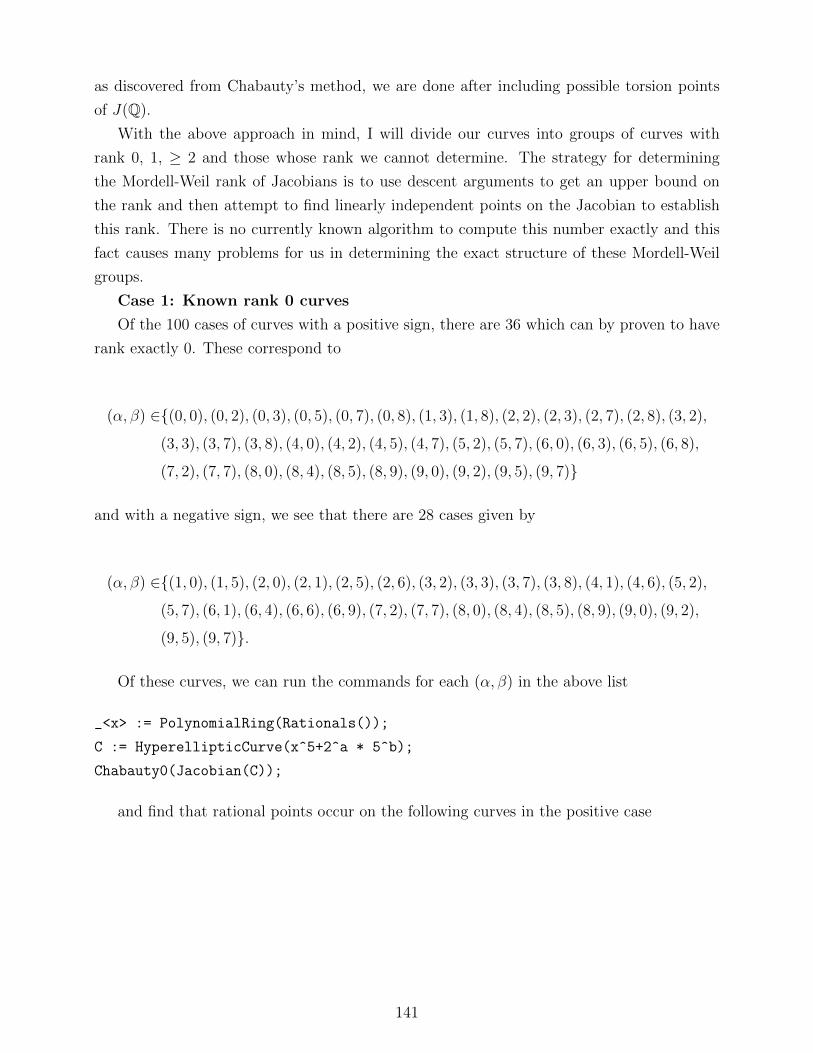
as discovered from Chabauty’s method, we are done after including possible torsion points
of J(Q).
With the above approach in mind, I will divide our curves into groups of curves with
rank 0, 1, ≥ 2 and those whose rank we cannot determine. The strategy for determining
the Mordell-Weil rank of Jacobians is to use descent arguments to get an upper bound on
the rank and then attempt to find linearly independent points on the Jacobian to establish
this rank. There is no currently known algorithm to compute this number exactly and this
fact causes many problems for us in determining the exact structure of these Mordell-Weil
groups.
Case 1: Known rank 0 curves
Of the 100 cases of curves with a positive sign, there are 36 which can by proven to have
rank exactly 0. These correspond to
(α, β) ∈(0, 0), (0, 2), (0, 3), (0, 5), (0, 7), (0, 8), (1, 3), (1, 8), (2, 2), (2, 3), (2, 7), (2, 8), (3, 2),
(3, 3), (3, 7), (3, 8), (4, 0), (4, 2), (4, 5), (4, 7), (5, 2), (5, 7), (6, 0), (6, 3), (6, 5), (6, 8),
(7, 2), (7, 7), (8, 0), (8, 4), (8, 5), (8, 9), (9, 0), (9, 2), (9, 5), (9, 7)
and with a negative sign, we see that there are 28 cases given by
(α, β) ∈(1, 0), (1, 5), (2, 0), (2, 1), (2, 5), (2, 6), (3, 2), (3, 3), (3, 7), (3, 8), (4, 1), (4, 6), (5, 2),
(5, 7), (6, 1), (6, 4), (6, 6), (6, 9), (7, 2), (7, 7), (8, 0), (8, 4), (8, 5), (8, 9), (9, 0), (9, 2),
(9, 5), (9, 7).
Of these curves, we can run the commands for each (α, β) in the above list
_<x> := PolynomialRing(Rationals());
C := HyperellipticCurve(x^5+2^a * 5^b);
Chabauty0(Jacobian(C));
and find that rational points occur on the following curves in the positive case
141

α β 2α5β (x, y)
0 0 1 (−1, 0)
0 0 1 (0,±1)
0 2 25 (0,±5)
0 5 3125 (−5, 0)
0 8 390625 (0,±625)
2 2 100 (0,±10)
2 8 1562500 (0,±1250)
4 0 16 (0,±4)
4 2 400 (0,±20)
6 0 64 (0,±8)
6 8 25000000 (0,±5000)
8 0 256 (0,±16)
8 4 160000 (0,±400)
8 5 800000 (20,±2000)
Table 3.10: Rational solutions to y2 = x5 + 2α5β for rank 0 curves
and in the negative case none of the curves have any rational points other than the point
at infinity.
Case 2: Known rank 1 curves
In this case, we discuss the situation where we know the generator of a curve with rank
1. The following list of coordinates give rise to such curves in the positive sign case
(α, β) ∈(0, 1), (0, 4), (1, 1), (1, 4), (1, 6), (2, 0), (2, 1), (2, 4), (2, 5), (3, 0), (3, 1), (3, 4), (4, 1),
(4, 4), (5, 0), (5, 1), (5, 4), (6, 1), (6, 4), (7, 0), (7, 1), (7, 4), (8, 2), (8, 3), (9, 1)
and in the negative sign case, we have
(α, β) ∈(0, 0), (0, 2), (1, 4), (2, 2), (3, 0), (3, 1), (4, 0), (4, 2), (5, 0), (5, 1), (6, 0), (6, 2), (8, 2).
There are also curves where the computation for the given model of our hyperelliptic
curves above go beyond what MAGMA can do. To handle these cases, we can change the
model to use smaller coefficients and this helps limit the search space to something more
manageable. There were six other cases in the positive sign setting given by
(α, β) ∈(0, 6), (2, 6), (3, 5), (5, 5), (7, 5), (8, 7)
142

and ten others in the negative sign setting given by
(α, β) ∈(0, 5), (0, 7), (0, 8), (2, 8), (4, 7), (6, 5), (7, 0), (7, 5), (8, 8), (9, 1)
where we can use the trick of changing the model to help us compute the Mordell-Weil group
of the Jacobian by reducing the size of the coefficients involved. It will turn out that we can
verify a generator in each of these cases as well.
To determine the Jacobian in these cases, we use MAGMA. To illustrate the methods
used above, I will show them explicitly using the curves y2 = x5 + 5 and y2 = x5 + 56. To
begin with the first curve, we set up the polynomial ring, the hyperelliptic curve and the
Jacobian.
> _<x> := PolynomialRing(Rationals());
> C := HyperellipticCurve(x^5 + 5);
> J := Jacobian(C);
> J;
Jacobian of Hyperelliptic Curve defined by y^2 = x^5 + 5 over Rational Field
We would like to know what the rank of this Jacobian is and for this we can use
“RankBounds”.
> RankBounds(J);
1 1
There is also a command called “RankBound” which just gives the upper bound. From this
we see that the lower and upper bounds of the Jacobian is indeed 1. Thus our curve has
rank 1. Next, we search for rational point on our curve up to some bound. We use the LLL
algorithm [LLL82] to help determine a basis of this group.
> ratPoints := RationalPoints(J:Bound:=5000);
> B := ReducedBasis(ratPoints);
> B;
[ (x + 1, 2, 1) ]
The point P = (x + 1, 2, 1) is on the Jacobian and MAGMA suggests that this could be
a possible generator. Remember that this point is in the Mumford representation (for more
details, see [Mul06]). To determine if this is the generator, we need to check the following.
Suppose that this was not the generator. Then there would be some point P0 such that
P = mP0 for some integer m. However, this m is an integer at least of size 2 and so using
143

the canonical height of the Jacobian (denoted by h) [HS00, p. 199] [Sto02b, Chapter 6], we
see that
h(P ) = h(mP0) = m2h(P0) ≤ 4h(P0).
This gives us that h(P0) ≤ 14h(P ) which in turn gives us a way to bound how far we need to
check for rational points. The command RationalPoints(J:Bound:=N) will look for rational
points up to naive height N on the associated Kummer Surface to our Jacobian (for more
details, see [CF96]). We can compute the maximum difference between the canonical height
and naive height using MAGMA and thus, to verify the bound, we need to check for rational
points up to the bound
exp
(h(P )
4+HC
)where HC is the height constant, this maximal height difference between canonical and naive
heights. For more details see [Sto99] [Sto02b]. Computing gives us that
> P := B[1];
> HC := HeightConstant(J:Effort:=2);
> hP := Height(P);
> boundToCheck := Exp(hP/4 + HC);
> boundToCheck;
11.1994504369602782170687264455
As we have already checked up to 5000, we have successfully determined that P is a
generator. In some cases, the computations are too large to be performed. For example,
consider the curve y2 = x5 + 56:
> C1 := HyperellipticCurve(x^5 + 5^6);
> J1 := Jacobian(C1);
> ratPoints1 := RationalPoints(J1:Bound:=15000);
> B1 := ReducedBasis(ratPoints1);
> B1;
[ (x^2 - 105/16*x - 525/16, 2205/64*x - 575/64, 2) ]
> HC1 := HeightConstant(J1:Effort:=2);
> hPoint := Height(B1[1]);
> Exp(hPoint/4+HC1);
57732.5711881962379928792966209
This computation just exceeds what MAGMA can do (the max bound rational points will
allow is 46340). We can reduce our model and perform this computation again. MAGMA has
a command that will give us a smaller model (though this is not an exact science - sometimes
other models can do better).
144

> C2, mapC1toC2 := ReducedMinimalWeierstrassModel(C1);
> C2;
Hyperelliptic Curve defined by y^2 = 5*x^5 + 25 over Rational Field
> J2 := Jacobian(C2);
> ratPoints2 := RationalPoints(J2:Bound:=1000);
> B2 := ReducedBasis(ratPoints2);
> HC2 := HeightConstant(J2: Effort:=2);
> hPoint2 := Height(B2[1]);
> Exp(hPoint2/4+HC2);
595.986306378025334312831604667
This computation is manageable. In our specific setting, we can also find a different model
by hand by using say (x, y) 7→ (2x, 22y) or (x, y) 7→ (5x, 52y) (or a combination of these
maps) provided that the power of α, β ≥ 4.
Next, we can execute Chabauty’s method on all these curves that we have computed
a Mordell-Weil basis for their respective Jacobians and come up with the following set of
solutions to the curves y2 = x5 ± 2α5β. To use the following command, we need to tell
MAGMA which prime specifically to check. This method returns the number of points that
are roots of the equation over Zp[[x]] discussed earlier modulo a prime power of p and taking
the cardinality of this set returns a bound on half the number of non-Weierstrass points. By
definition, Weierstrass points are the points (x, 0) and the point at infinity. We also need to
check the torsion subgroup for any other points not coming from the free part of J(Q). In
our example y2 = x5 + 5, we have
// Recall C := HyperellipticCurve(x^5 + 5)
> RationalPoints(C:Bound:=1000000);
@ (1 : 0 : 0), (-1 : -2 : 1), (-1 : 2 : 1) @
> TorsionSubgroup(J);
Abelian Group of order 1
Mapping from: Abelian Group of order 1 to JacHyp:
J given by a rule [no inverse]
We can see that we do not have any points coming from the torsion subgroup and we
only have one non-Weierstrass point given by (−1,±2). Since we know two non-Weierstrass
points on our curve, we are done if our Chabauty method returns the value 1.
//Recall P := B[1];
> #Chabauty(P,7);
2
145

> #Chabauty(P,11);
5
> #Chabauty(P,13);
1
We reach our bound using the prime p = 13. Thus we can conclude that the number of
rational points on y2 = x5 + 5 is exactly 2 given by (−1 ± 2). We repeat this computation
on all the curves y2 = x5 + 2α5β that have rank 1 to illustrate this method. The column
denoted by p denotes the prime used in Chabauty.
α β C(Q)\∞ p
0 1 (−1,±2) 13
0 4 (0,±25) 11
0 6 (0,±125) 7
1 1 (−1,±3) 11
1 4 11
1 6 11
2 0 (0,±2), (2,±6) 19
2 1 29
2 4 (0,±50), (5,±75) 61
2 5 (5,±125) 19
2 6 (0,±250) 11
3 0 (1,±3) 13
3 1 11
3 4 31
3 5 17
4 1 (1,±9) 19
α β C(Q)\∞ p
4 4 (0,±100) 11
5 0 (−2, 0), (2,±8) 109
5 1 17
5 4 19
5 5 (−10, 0) 11
6 1 17
6 4 (0,±200), (20,−1800) 229
7 0 11
7 1 29
7 4 59
7 5 11
8 2 (0,±80) 11
8 3 (−4,±176) 11
8 7 17
9 1 19
Table 3.11: Rational points on y2 = x5 + 2α5β for known rank 1 curves.
In the later versions of MAGMA, we can also perform Chabauty, the Mordell-Weil sieving
and the torsion computation without explicitly giving the primes needed to check. This can
be done using
> Chabauty(P); //Recall P is the generator of J.
(-1 : -2 : 1), (1 : 0 : 0), (-1 : 2 : 1)
3, 19, 29, 59, 79
[ 5, 2, 3, 2 ]
146

The first line is the list of rational points. The next two are Mordell-Weil sieving data
which we will not discuss here. This helps to take care of ghost solutions as in [Mul06, p.191]
and [BC06, p.63-92]. Using this command, we do likewise for the curve y2 = x5 − 2α5β and
see that
α β C(Q)\∞0 0 (1, 0)
0 2
0 5 (5, 0)
0 7
0 8
1 4
2 2 (5,±55)
2 8
3 0
3 1
4 0 (2,±4)
4 2
α β C(Q)\∞4 5
4 7
5 0 (2, 0), (6,±88)
5 1
6 0
6 2
6 5
7 0
7 5
8 2
8 8
9 1
Table 3.12: Rational points on y2 = x5 − 2α5β for known rank 1 curves.
3.2.2 Elliptic Curve Chabauty
We now address the question of what happens when Chabauty’s method cannot be applied
either because the rank of J(Q) is greater than 1 or because we cannot specifically compute
the exact size of the rank. In this case, there are some more advanced techniques that one
can try to use (see also [Mul06], [Sto98] and [Sto02a] for other tricks, but the ones mentioned
there do not work here). The first of which is Elliptic Curve Chabauty. The idea behind
this method is to pass our curves to a covering collection of curves that map down to elliptic
curves over a relatively small number field K. Over this number field, we try to find all
points where the x component is rational. These give a superset of all the rational points
on our elliptic curve. One can then map these points back to the original curve and verify
whether or not they are rational points for our original curve. For more details, see [Bru02]
and [Bru03].
Our first step is to get this covering collection. A common way to do this is to use a
147

2-cover descent. The main idea here is to write our hyperelliiptic curve C/K as
C : y2 = f(x) = g(x)h(x) = fn
deg(f)∏i=1
(x− θi)
where h(x) is monic (for us it will be a monic linear term), g(x) is of even degree and
g(x), h(x) ∈ L[x] for some finite extension L of K and fn is the coefficient of xn in f(x).
For our applications here our f(x) is a degree five monic polynomial and so we make this
simplifying assumption. For more details on any of these methods in full generality, the
reader is encouraged to see [BS08], [BS09] and [BS10].
Define HK := δ ∈ A∗/A∗2 : NA/K(δ) ∈ k∗2 where A = K[x]/f(x) = K[θ] for θ = θ1.
For δ ∈ HK , we can write down the cover given by
Dδ =
y21 = δ1(x− θ1)
...
y25 = δ5(x− θ5)
y = y1...y5
1 = δ1...δ5
where here we are thinking of δ1, ..., δ5 as conjugates of δ and hence we think of y1, ..., y5 as
conjugates as well. Condensing the above map and relabeling gives
Eγ : γy21 = g(x)
E′
γ : (1/γ)y22 = h(x)
where this γ is associated to the δ from above as follows. Suppose that δ ∈ A and let
L[Θ] = L[x]/h(x). Define the map
j : A→ L[Θ]
θ 7→ Θ
and extend the above map in the natural way. Then, we have that γ = NL[Θ]/L(j(δ)). Denote
this γ by γ(δ) to remind ourselves of the association. The question now arises “How many
of these such δ (and consequently γ(δ)) values do we have to consider?” The smallest such
set we can hope to obtain by purely local means is given by the fake 2-Selmer group. This is
148

defined as follows. The map from A→ A⊗K Kv gives a commutative diagram
C(K)µK> HK
C(Kv)∨
µKv> HKv
ρKv∨
From here, we define the fake 2-Selmer group as
Sel(2)fake(C/K) = δ ∈ HK : ρKv ∈ µKv(C(Kv)) for all places v ∈ K.
This group was first introduced by Poonen and Schaefer [PS97]. It is related to the Selmer
group by being equal to a quotient of the Selmer group. For more details on this, see
[SvL13]. With all this terminology now introduced, we can note that there is an algorithm for
computing the fake 2-Selmer group and this has been implemented in MAGMA. Proceeding
with the computation gives
> P<x> := PolynomialRing(Rationals());
< poly := x^5 + 2*5^5;
> C := HyperellipticCurve(poly);
> Hk,AtoHk := TwoCoverDescent(C);
> Hk := [d @@ AtoHk : d in Hk];
> Hk;
[
1,
-1/5*theta - 1
]
> K<w> := NumberField(poly);
> HK := [Evaluate(P!d, w) : d in Hk];
> HK;
[
1,
1/5*(-w - 5)
]
This means that every rational point on our curve C leads to a rational point with the
same Q-rational x-coordinate on one of the two genus 1 curves given by
E1 : y2 = g(x)
E2 : y2 = −1/5(w + 5)g(x)
149

where g(x) := x5+2·55x−w . We load this now into MAGMA
> PK<X> := PolynomialRing(K);
> g := ExactQuotient(Evaluate(PK!poly,X), X - w);
We will run Elliptic Curve Chabauty on each elliptic curve. To do this, we iterate over all
values of “HK” and use MAGMA’s built-in capabilities. First we set up our elliptic curve.
> for d in HK do
for> C2 := HyperellipticCurve(d*g);
for> E, mE := EllipticCurve(C2, RationalPoints(C2:Bound:=20)[1]);
Here we might need some user intervention depending on if we cannot find any small rational
points. If you know a rational point on the curve, for example infinity when d = 1 and x = 15
when d = −1/5(w + 5), then you can use the command
for> Rep(Points(C2, Infinity()))
instead of searching for rational points. With the elliptic curve built, we can now attempt
to compute the rank. This command can take a bit of time depending on the curve. For the
purposes of showing sample output, I will assume that d = −1/5(w+ 5) and that we use the
point at x = 15.
for> E, mE := EllipticCurve(C2, Rep(Points(C2, 15)));
for> bounds, gens := MordellWeilShaInformation(E);
for> end for;
Torsion Subgroup = Z/2
The 2-Selmer group has rank 3
Found a point of infinite order.
Found 2 independent points.
After 2-descent:
2 <= Rank(E) <= 2
Sha(E)[2] is trivial
(Searched up to height 16 on the 2-coverings.)
It is here that we should note we need the rank above to be exact. If we cannot compute
the exact rank of E then we cannot guarantee that the next steps are valid. Here we know
rank(E) = 2 and so we can continue to apply Elliptic Curve Chabauty since this rank is
less than the degree of the number field extension (which is 5). Next, we set up an abstract
representation of the Mordell-Weil group of E.
150

> T, mapTtoE := TorsionSubgroup(E);
> A := AbelianGroup(Invariants(T) cat [0 : g in gens]);
> gensE := [mapTtoE(T.j) : j in [1..Ngens(T)]] cat gens;
> MWmap := map<A -> E | a :-> &+[e[i]*gensE[i] : i in [1..#e]]
where e := Eltseq(a)>;
> MWmap;
Mapping from: GrpAb: A to CrvEll: E given by a rule [no inverse]
Some notes on the above code. The code “T.j” refers to the elements of T (and in partic-
ular the generators). The symbols “& +” will take the map on each of the generators and put
them together to form an element in E. Elliptic Curve Chabauty requires a representation of
the Mordell-Weil group and a map from E to P1. The major idea is the following. Let C/K
be an algebraic curve where K is a number field. Suppose that C covers an elliptic curve
E defined over L where L is a finite extension of K. Next, consider following commutative
diagram
Cφ> E
P1
π∨Φ >
where Φ is defined over K and φ, π are defined over L. The map φ is the aforementioned
cover of E. From this map, we can see that
Φ(C(K)) ⊆ φ(E(L)) ∩ P1(K)
The right most set can sometimes be bounded using p-adic methods. One such situation is
when rank(E) ≤ [L : K]. The details of this method can be found in [Bru02] and [Bru03]. If
the bound is sharp, then we have found all rational points on C. For our purposes, MAGMA
has the built in functionality and so we will not go into the details. We compute the necessary
values as follows.
> P1 := ProjectiveSpace(Rationals(), 1);
> piC2toP1 := map<C2 -> P1 | [FunctionField(C2).1,1]>;
> piE := Inverse(mE)*piC2toP1;
> set, n := Chabauty(MW, piE);
> set, n;
0,
$.1 + $.2 - $.3,
$.1 + $.2 - 3*$.3,
151

-2*$.3
396902628105984000
Lastly, we need to verify that the output is valid. This is the case if the index of A in
E(K) is finite and coprime to n as computed in the above code. This can be done using the
“Saturation” command.
> primes := PrimeDivisors(n);
> p := 1;
> omitPrimes := [];
> while(p lt (Max(primes)+1)) do
while> p := NextPrime(p);
while> if not(p in primes) then
while|if> omitPrimes := Append(omitPrimes,p);
while|if> end if;
while> end while;
> sat := Saturation(gens, Max(primes) :
TorsionFree, OmitPrimes := omitPrimes);
> sat eq gens;
True
The “Saturation” command takes in rational points on E and an integer n and returns a
sequence of points generating a subgroup of E(Q) such that the given points are contained
in the subgroup and that the subgroup is p-saturated for all primes p up to n excluding those
given by the optional “OmitPrimes” parameter. Recall that a subgroup S is p-saturated in a
group G if there is no intermediate subgroup H for which the index in S is finite and divisible
by p. This is the exact condition we wish to verify. If “TorsionFree” is specified above to be
true, then the torsion points are omitted from the result. Checking this to be equal to the
generators is enough.
If this last check of equality with the generators turns out to be false, then use the
saturated group in place of the original generators (in our case given by “gens”) and repeat
the computation. Check that the new second value does not have new prime divisors or else
repeat the saturation step with the new primes and loop until you get an equality.
Translating back to the curve C, we see that the rational points on C corresponding to
d = −1/5(w + 5) are given by
> xCoords := piE(MW(s)) : s in set;
> ptsOnC := &joinPoints(C, pt[2] eq 0 select Infinity() else pt[1]/pt[2]) :
152
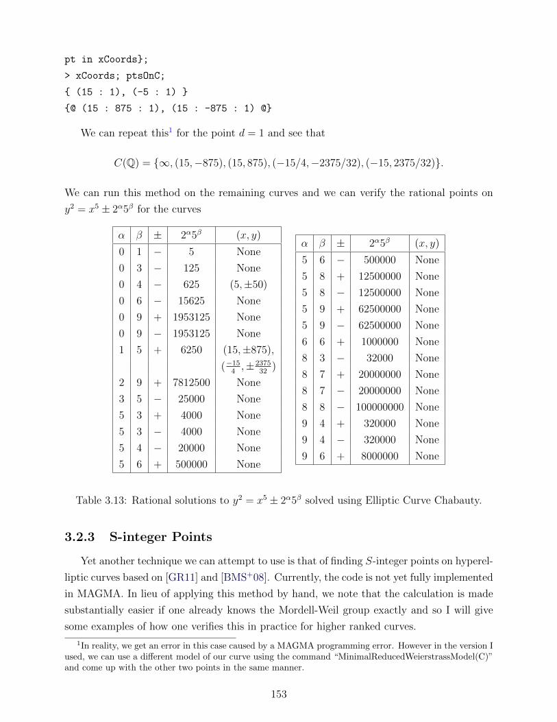
pt in xCoords;
> xCoords; ptsOnC;
(15 : 1), (-5 : 1)
@ (15 : 875 : 1), (15 : -875 : 1) @
We can repeat this1 for the point d = 1 and see that
C(Q) = ∞, (15,−875), (15, 875), (−15/4,−2375/32), (−15, 2375/32).
We can run this method on the remaining curves and we can verify the rational points on
y2 = x5 ± 2α5β for the curves
α β ± 2α5β (x, y)
0 1 − 5 None
0 3 − 125 None
0 4 − 625 (5,±50)
0 6 − 15625 None
0 9 + 1953125 None
0 9 − 1953125 None
1 5 + 6250 (15,±875),
(−154,±2375
32)
2 9 + 7812500 None
3 5 − 25000 None
5 3 + 4000 None
5 3 − 4000 None
5 4 − 20000 None
5 6 + 500000 None
α β ± 2α5β (x, y)
5 6 − 500000 None
5 8 + 12500000 None
5 8 − 12500000 None
5 9 + 62500000 None
5 9 − 62500000 None
6 6 + 1000000 None
8 3 − 32000 None
8 7 + 20000000 None
8 7 − 20000000 None
8 8 − 100000000 None
9 4 + 320000 None
9 4 − 320000 None
9 6 + 8000000 None
Table 3.13: Rational solutions to y2 = x5 ± 2α5β solved using Elliptic Curve Chabauty.
3.2.3 S-integer Points
Yet another technique we can attempt to use is that of finding S-integer points on hyperel-
liptic curves based on [GR11] and [BMS+08]. Currently, the code is not yet fully implemented
in MAGMA. In lieu of applying this method by hand, we note that the calculation is made
substantially easier if one already knows the Mordell-Weil group exactly and so I will give
some examples of how one verifies this in practice for higher ranked curves.
1In reality, we get an error in this case caused by a MAGMA programming error. However in the version Iused, we can use a different model of our curve using the command “MinimalReducedWeierstrassModel(C)”and come up with the other two points in the same manner.
153

Contrary to the rank 1 case where we could do a simple computation involving the height
constant and one fourth the value of the presumed generator, when we consider ranks 2
or higher we need to use more sophisticated machinery [Sto02b]. The main idea here is to
compute a value called the covering radius % (or at least an upper bound on it). Once we
have this value, we use an upper bound similar to that in the rank 1 case to check that there
are no more rational points on the Jacobian of naive height at most
exp(%2 +HC
)where again HC is the height constant. We illustrate this method using the curves y2 =
x5 − 2453 and y2 = x5 − 2459. First we proceed with the second curve which has rank 2 as
given by
> _<x> := PolynomialRing(Rationals());
> C := HyperellipticCurve(x^5 - 2^4*5^9);
> C1, mapCtoC1 := ReducedMinimalWeierstrassModel(C); C1;
Hyperelliptic Curve defined by y^2 = -5*x^6 + 50*x over Rational Field
> J1 := Jacobian(C1);
> B := ReducedBasis(RationalPoints(Jacobian(C1):Bound:=8000));
> B;
[ (x^2 + x + 18/7, 9/7*x + 12/7, 2),
(x^2 + 17/3*x + 32/3, 1/9*x + 712/9, 2) ]
Then to compute the covering radius, we use the formula found in [Sto02b, p. 178] as
given by
%2 =h(P1)h(P2)h(P1 ± P2)
4Reg(P1, P2)
where Reg denotes the regulator and the sign above is chosen to give the smaller value of
h(P1 ± P2). If we use the height pairing matrix M = (〈Pi, Pj〉)1≤i,j≤2 where
〈Pi, Pj〉 =h(P1 + P2)− h(P1)− h(P2)
2
we can also see that
%2 =〈P1, P1〉〈P2, P2〉(〈P1, P1〉+ 〈P2, P2〉+ 2|〈P1, P2〉|)
4 det(M)
valid since h(P1 + P2)− h(P1 − P2) = 2(h(P1) + h(P2)). This gives
> H1 := HeightPairingMatrix(B);
> H1;
154

[5.70203132416513267250593814558 0.607244504928574524217534640890]
[0.607244504928574524217534640890 8.21959988070301859177146320080]
> rsq := H1[1,1]*H1[2,2]*(H1[1,1]+H1[2,2]-2*Abs(H1[1,2])
/(4*Determinant(H1));
> rsq;
3.20197769760017634737894478458
> HC := HeightConstant(J1 : Effort := 2);
> Exp(HC + rsq);
7604.25353647160094586160852567
This confirms that our generators for J(Q) are given by
(x2 + x+ 18/7, 9x/7 + 12/7, 2), (x2 + 17x/3 + 32/3, x/9 + 712/9, 2).
If we pull back, we see that the generators are
> C5 := HyperellipticCurve(x^5 - 2^4*5^9);
> C10, mapping := ReducedMinimalWeierstrassModel(C5);
> basOrig := [Pullback(mapping,b) : b in B];
> basOrig;
[ (x^2 - 175/9*x + 8750/9, 1225/27*x - 16250/27, 2),
(x^2 - 425/16*x + 1875/8, -47525/64*x + 314375/32, 2) ]
With rank 3 and higher, there is no exact formula like in the r = 2 case. However MAGMA
is still capable of computing this. We perform this computation for our only rank 3 curve
given by y2 = x5 − 2453. As always, we produce potential candidates for our generators.
> _<x> := PolynomialRing(Rationals());
> C2 := HyperellipticCurve(x^5 - 2^4*5^3);
> C3, mapC2toC3 := ReducedMinimalWeierstrassModel(C2); C3;
Hyperelliptic Curve defined by y^2 = 2*x^5 - 125 over Rational Field
> J3 := Jacobian(C3);
//Can take a while
> B3 := ReducedBasis(RationalPoints(Jacobian(C3):Bound:=24500));
> B3;
[(x - 3, 19, 1), (x - 7, 183, 1), (x^2 + 1/2*x + 3/2, 19/2*x + 5/2, 2) ]
Next, we compute the covering radius. This is done by using the height pairing matrix
as before, creating a lattice from the matrix and then computing the covering radius.
> H3 := HeightPairingMatrix(B3);
155

> L3 := LatticeWithGram(H3);
> r3 := CoveringRadius(L3);
Runtime error in ’CoveringRadius’: Argument 1 must be over Z or Q
The problem with this code is that the height pairing matrix is over a real field of precision
30. In order to compute the covering radius, we must tell MAGMA to think of “H3” as a
rational matrix. To do this, we truncate the entries at a few different values for n and then
we compute the covering radius. Note that the command “CoveringRadius” runs in time
approximately factorial in the size of the matrix and so is really only feasible for small values
of the size of the matrix.
> seq := [];
> n := 8; //Vary for precision
>for a in [1,2,3] do
> for b in [1,2,3] do
//Trick to round values multiply by power of 10, floor, then divide.
> seq := Append(seq,Floor((10^n)*H[a][b])/10^n);
> end for;
>end for;
> H3 := Matrix(RationalField(),3,3,seq);
> L3 := LatticeWithGram(H3);
> r3 := CoveringRadius(L3);
> r3;
2.27285021881299
If we vary the n values from say 1 to 10, we can see that %2 ≤ 2.3. This gives
> HC := HeightConstant(Jacobian(C):Effort:=2);
> Exp(2.3^2 + HC);
24116.3154447130917357362220427
and we have already verified past this bound so our basis is given by
(x− 3, 19, 1), (x− 7, 183, 1), (x2 + x/2 + 3/2, 19x/2 + 5/2, 2).
Now that one has these points, one could in principle use the techniques of [GR11] to find
the S-integral points on this curve. In order to use this technique, one need only two more
facts, namely a bound on the number of S-integral points of the curve and a variant of the
Mordell-Weil Sieve capable of searching up to the bounds. I will not do this here because
the Mordell-Weil Sieving code still requires some in depth user knowledge before executing
156

properly which the author has yet to obtain. I will however state that there is no reason that
this technique could not be done if the user had enough knowledge of the code (or enough
time to write his or her own). We will see in the section on Thue-Mahler equations that
work has already been done to classify the integer points on these two curves and that will
be enough for our purposes.
3.2.4 Other Techniques
We can also use elliptic curves in the rare case that the polynomial on the right factors.
For example, for
y2 = x5 − 2555 = (x− 10)(x4 + 10x3 + 100x2 + 1000x+ 10000),
we have that the factors on the right are coprime and hence we can use techniques for finding
2, 5∞-integral points on the elliptic curve
y2 = x4 + 10x3 + 100x2 + 1000x+ 10000.
We use MAGMA via the command
//The following command includes integral points
> SIntegralQuarticPoints([1,10,100,1000,10000], [2,5]);
[
[ 30, -1100 ],
[ -10, -100 ],
[ -55/4, 2525/16 ],
[ 0, 100 ]
]
A quick check shows that none of these points leads to a 2, 5,∞-integer point on y2 =
x5− 2555. Thus the only such point must come when y = 0 and hence x = 10. This gives us
that the only 2, 5-integer points on this curve is the point (x, y) = (10, 0).
3.2.5 Integer Points Via Thue-Mahler Equations
When the previous methods fail one can always try to simplify the search by trying to find
integer solutions to your equations. The goal of this section is to compute integer solutions
to y2 = x5±2α5β with α, β ≥ 0. Our primary tools will be techniques from algebraic number
theory as well as reductions to Thue-Mahler equations, that is, equations of the form
f(x, y) = cpz11 ...pznn
157

where f(x, y) is an irreducible binary form in Z[x, y] of degree at least 3. From here, we apply
an algorithm of [TdW92] as implemented by [Ham11] to solve these equations. Throughout
we assume that xy 6= 0 as these solutions are easy to obtain. In this case, we know that
the greatest common divisor of x and y has only powers of 2 and 5. Thus, removing all the
powers of 2 and 5 in x and y, let
y = 2y15y2 y
x = 2x15x2x.
Plugging this into our equation, we have
22y152y2 y2 = 25x155x2x5 ± 2A5B.
Notice that two of the powers of 2 must be equal and the third must be a larger power of
the smaller two. This leads to the following cases:
1. 2y1 = 5x1 and 2y2 = 5x2
2. 2y1 = 5x1 and 2y2 = B
3. 2y1 = 5x1 and 5x2 = B
4. 2y1 = A and 2y2 = 5x2
5. 2y1 = A and 2y2 = B
6. 2y1 = A and 5x2 = B
7. 5x1 = A and 2y2 = 5x2
8. 5x1 = A and 2y2 = B
9. 5x1 = A and 5x2 = B.
We proceed case by case. Note in all the cases below, the class number is coprime to 5 and
so factoring in the ring of integers will be permitted.
1. 2y1 = 5x1 and 2y2 = 5x2.
This case is equivalent to gcd(x, y) = 1. For the duration of this case, to easy notation,
we suppose that we have a solution to y2 = x5± 2α5β with gcd(x, y) = 1. The work for
the equation with a negative sign has been done as a consequence of the following.
Theorem 3.2.6. [GLT08] (Goins, Luca, Togbe) The only solutions to y2 = x5 −2α5β for gcd(x, y) = 1 and α, β non-negative integers are given by (x, y, α, β) =
(11,±401, 1, 3) or (x, y, α, β) = (1, 0, 0, 0).
158
This was done using work on Lucas sequences and S-integral points on elliptic curves.
For the rest of this section, we attempt to apply a myriad of techniques to the equation
y2 = x5 + 2α5β with gcd(x, y) = 1 to come up with a full solution set to the above
problem. We attempt to solve this first by factoring.
Case 1: Suppose that α = 2a and β = 2b for some non-negative integers a and b.
Then we have (y − 2a5b)(y + 2a5b) = x5. Now, let d = gcd(y − 2a5b, y + 2a5b). Adding
the two values shows that d | 2y. Now if d | y, then d | 2α5β and so d | x, contradicting
the coprimality of x and y. If d = 2 then we know that 2 - y from the above argument
and so we must have that a = 0 when d = 2. The argument to follow only works when
d = 1 and so we assume that a 6= 0. The case where a = 0 was solved earlier using
Chabauty’s method. Unique factorization tells us that
y − 2a5b = M5 and y + 2a5b = N5
and so subtracting gives N5 + (−M)5 = 2a5b. Using Theorem 1.6.2 (valid since the
right hand side is a square), we have that the only solution to x5 + y5 = Cz2 for
C ∈ 1, 2, 5, 10 with x > y is given by C = 2 and (n, x, y, z) = (5, 3,−1,±11). Since
here z is a power of 2 and 5 in our situation, we have a contradiction. Summarizing
gives
Lemma 3.2.7. There are no solutions to y2 = x5 + 2α5β with α, β even non-negative
integers with α > 0 and x, y coprime integers.
This technique worked because we could factor in a unique factorization domain. We
now attempt to try this over the ring Z(√
2) which is also a unique factorization domain.
Case 2: We assume now that α = 2a + 1 and β = 2b. Performing a factorization in
Z[√
2] gives us (y−2a5b√
2)(y+2a5b√
2) = x5. Again, let d = gcd(y−2a5b√
2, y+2a5b√
2)
for d ∈ Z[√
2]. Adding the two values shows that d | 2y. Now if d | y, then d | 2α5β
and so d | x thus d = 1. If d = 2 then as d | 2a5b√
2, we have that d | y and the above
again shows that d | x, a contradiction. Unique factorization tells us that
y + 2a5b√
2 = (1 +√
2)k(m+ n√
2)5 (3.1)
where m,n ∈ Z, 1 +√
2 is a fundamental unit for Z[√
2] and we have absorbed roots
of unity into the 5th power. We may suppose without loss of generality that 0 ≤ k ≤ 4
since we can absorb all the 5th powers into the (m + n√
2)5 term if necessary. Using
the first equation above, we can expand and compare coefficients of√
2 to get a set of
159

equations for each value of k given by fk(m,n) = 2δ15δ2 given by
k = 0 f0(m,n) := n(5m4 + 20m2n2 + 4n4)
k = 1 f1(m,n) := m5 + 5m4n+ 20m3n2 + 20m2n3 + 20mn4 + 4n5
k = 2 f2(m,n) := 2m5 + 15m4n+ 40m3n2 + 60m2n3 + 40mn4 + 12n5
k = 3 f3(m,n) := 5m5 + 35m4n+ 100m3n2 + 140m2n3 + 100mn4 + 28n5
k = 4 f4(m,n) := 12m5 + 85m4n+ 240m3n2 + 340m2n3 + 240mn4 + 68n5.
To solve this, we use the Thue-Mahler solver. The program takes as an input an
irreducible binary form of degree at least 3, a parameter and a set of primes given by
a tuple ([c0, ..., cn], [p1, ..., pk], A) where
c0XN + c1X
N−1Y + ...+ cNYN = ±Apδ11 · · · p
δkk
and outputs coprime integers X, Y with gcd(c0, Y ) = 1 satisfying the above equation.
First, let’s see why solving for solutions with gcd(X, Y ) = 1 is not an issue. Notice that
for a solution (m0, n0) to our Thue-Mahler equation above implies that gcd(m0, n0) | yby Equation 3.1. As gcd(m0, n0) | 2a5b, we must also have that gcd(m0, n0) | x as well.
So gcd(m0, n0) | gcd(x, y) = 1 showing that gcd(m0, n0) = 1 since we assumed that x
and y were coprime. Thus solving the Thue-Mahler equation for coprime m and n is
sufficient.
For our purposes, the restriction that gcd(c0, Y ) = 1 is unwanted so to deal with this,
we solve the following set of related Thue-Mahler equations gj(m,n) = ±2δ15δ2 where
gj(m,n) are given by [Ham11, p.6]
k = 0 g1(m,n) := 5m4 + 20m2n2 + 4n4
k = 0 g2(m,n) := m4 + 100m2n2 + 500n2
k = 1 g3(m,n) := m5 + 5m4n+ 20m3n2 + 20m2n3 + 20mn4 + 4n5
k = 2 g4(m,n) := 2m5 + 15m4n+ 40m3n2 + 60m2n3 + 40mn4 + 12n5
k = 2 g5(m,n) := m5 + 15m4n+ 80m3n2 + 240m2n3 + 320mn4 + 192n5
k = 3 g6(m,n) := 5m5 + 35m4n+ 100m3n2 + 140m2n3 + 100mn4 + 28n5
k = 3 g7(m,n) := m5 + 35m4n+ 500m3n2 + 3500m2n3 + 12500mn4 + 17500n5
k = 4 g8(m,n) := 12m5 + 85m4n+ 240m3n2 + 340m2n3 + 240mn4 + 68n5
k = 4 g9(m,n) := 6m5 + 85m4n+ 480m3n2 + 1360m2n3 + 1920mn4 + 1088n5
k = 4 g10(m,n) := 3m5 + 85m4n+ 960m3n2 + 5440m2n3 + 15360mn4 + 17408n5.
160

To give an idea of the above collection and where they come from, take the case with
k = 0 above. To go to the second k = 0 case, multiply every term by 53 and then
relabel mnew = 5m. Each time you do this you will find solutions with d | y where d is
the base of the number we are multiplying by. For example, solving with j = 9 above,
we see that we will find solutions to our original Thue-Mahler equation with 2 | n and
solving with j = 10 above, we see that we will find solutions to our original Thue-
Mahler equation with 4 | n. Solving the above sets of equations gives the following
solutions.
j Solutions to gj(m,n) = ±2δ15δ2 in the form (m,n, δ1, δ2)
1 (1, 0, 0, 1), (−1, 0, 0, 1)
2 (1, 0, 0, 0), (−1, 0, 0, 0)
3 (1, 0, 0, 0), (−1, 0, 0, 0)
4 (−1, 1, 0, 1), (1,−1, 0, 1)
5 (−2, 1, 4, 1), (2,−1, 4, 1), (1, 0, 0, 0), (−1, 0, 0, 0)
6 (−1, 1, 1, 0), (1,−1, 1, 0)
7 (−1, 0, 0, 0), (1, 0, 0, 0), (−5, 1, 1, 4), (5,−1, 1, 4)
8 (−1, 1, 0, 0), (1,−1, 0, 0), (−2, 1, 2, 0), (2,−1, 2, 0)
9 (2,−1, 4, 0), (−2, 1, 4, 0), (−4, 1, 6, 0), (4,−1, 6, 0)
10 (4,−1, 8, 0), (−4, 1, 8, 0), (−8, 1, 10, 0), (8,−1, 10, 0)
Table 3.14: Solutions to gj(m,n) = ±2δ15δ2 with gcd(m,n) = 1 and n coprime to the
coefficient of gj(m, 0).
Notice that in the cases of j = 4 and j = 6 above, we get only one more additional
solution to our original equation with gcd(c0, Y ) > 1 and these come when Y = 0. To
satisfy gcd(X, Y ) = 1, we have that only (m,n) = (±1, 0) are added solutions given
from this reduction process. Our k = 0 situation above does not give us a valid solution
since the coefficient of√
2 on the left is nonzero. Thus our final list of solutions for
fk(m,n) = 2α5β is as follows:
161

k Solutions to fk(m,n) = 2δ15δ2 in the form (m,n, δ1, δ2) Corresponding (x, y, α, β)
0 None None
1 (1, 0, 0, 0) (−1, 1, 1, 0)
2 (−1, 1, 0, 1) (−1,−7, 1, 2)
2 (1, 0, 0, 0) (1, 3, 3, 0)
3 (1,−1, 1, 0) (1,−3, 3, 0)
3 (1, 0, 0, 0) (−1, 7, 1, 2)
4 (−1, 1, 0, 0) (−1,−1, 1, 0)
4 (−2, 1, 2, 0) (2,−8, 5, 0)
Table 3.15: Solutions to fk(m,n) = 2δ15δ2 with gcd(m,n) = 1 and n coprime to the coefficient
of gj(m, 0).
To compute the last column above, we plug back in (m,n) into the Equation 3.1
and solve for the corresponding variables. Notice that the last solution, we obtain a
solution with gcd(x, y) > 1. Notice that finding solutions with gcd(m,n) = 1 does not
necessarily guarantee finding solutions with gcd(x, y) = 1 but it does ensure that we
find all such solutions with gcd(x, y) = 1. Summarizing the above, we get the following
Lemma 3.2.8. Solutions to y2 = x5 + 2α5β with α, β non-negative integers with α odd
and β even and x, y coprime integers are given by the following
(x, y, α, β) ∈ (−1,±1, 1, 0), (−1,±7, 1, 2), (1,±3, 3, 0)
Case 3: We assume now that α = 2a and β = 2b + 1. Notice that Z[√
5] is not a
unique factorization domain, however Z[1+√
52
] is. Performing a factorization in Z[1+√
52
]
gives us (y − 2a5b√
5)(y + 2a5b√
5) = x5. Again, let d = gcd(y − 2a5b√
5, y + 2a5b√
5)
for d ∈ Z[1+√
52
]. Adding the two values shows that d | 2y. Now if d | y, then d | 2α5β
and so d | x thus d = 1. If d = 2 then we know from above that d - y and so α = 0 and
y is odd. Thus x is even and modulo 8, we have that
y2 = x5 + 2α5β ≡ 0 + 52b+1 ≡ 5 (mod 8)
which is a contradiction since odd squares modulo 8 are congruent to 1. Thus we have
that d = 1 and so unique factorization tells us that
y + 2a5b√
5 =
(1 +√
5
2
)k(m+ n
√5
2
)5
(3.2)
162

where m,n ∈ Z, 1+√
52
is a fundamental unit for Z[1+√
52
] and we have absorbed roots
of unity into the 5th power. As before, we may suppose without loss of generality that
0 ≤ k ≤ 4.
In contrast to the previous situation where we had leading coefficients that might
have shared prime divisors with the n value, we do not have coefficients that are no
longer necessarily integers. To simplify this we’ll multiply through to eliminate the
denominators (notice that our set of primes already contains 2 so this introduces no
additional concerns). This can give us additional solutions depending on how big the
power of 2 is. Evaluating the powers of the fundamental unit, we see that1 +√
5
2
k=4
k=0
=
1,
1 +√
5
2,3 +√
5
2, 2 +
√5,
7 + 3√
5
2
.
From this, we see when k = 0, 3, then we can multiply by 25 to clear denominators
and in the other three k cases, we multiply by 26 to clear denominators. This gives the
following quintic forms fk(m,n) = 2δ15δ2 after expanding and comparing coefficients of√5.
k = 0 g0(m,n) := 25f0(m,n)/(5n) := m4 + 10m2n2 + 5n4
k = 1 g1(m,n) := 26f1(m,n) := m5 + 5m4n+ 50m3n2 + 50m2n3 + 125mn4 + 25n5
k = 2 g2(m,n) := 26f2(m,n) := m5 + 15m4n+ 50m3n2 + 150m2n3 + 125mn4 + 75n5
k = 3 g3(m,n) := 25f3(m,n) := m5 + 10m4n+ 50m3n2 + 100m2n3 + 125mn4 + 50n5
k = 4 g4(m,n) := 26f4(m,n) := 3m5 + 35m4n+ 150m3n2 + 350m2n3
+ 375mn4 + 175n5.
Solving using the Thue-Mahler solver, we have
j Solutions to gj(m,n) = ±2δ15δ2 in the form (m,n, δ1, δ2)
0 (−1, 0, 0, 1), (1, 0, 0, 1), (1,−1, 4, 1), (−1, 1, 4, 1), (1, 1, 4, 1)(−1,−1, 4, 1)
1 (−1, 0, 0, 0), (1, 0, 0, 0), (0, 1, 0, 2), (0,−1, 0, 2), (1, 1, 8, 0), (−1,−1, 8, 0)
2 (−1, 0, 0, 0), (1, 0, 0, 0), (−1, 1, 6, 0), (1,−1, 6, 0), (−5, 1, 7, 2), (5,−1, 7, 2)
3 (−1, 0, 0, 0), (1, 0, 0, 0), (0,−1, 1, 2), (0, 1, 1, 2)
4 (1,−1, 5, 0), (−1, 1, 5, 0), (3,−1, 8, 0), (−3, 1, 8, 0), (−5, 1, 5, 2), (5,−1, 5, 2)
Table 3.16: Solutions to gj(m,n) = ±2δ15δ2 with gcd(m,n) = 1 and n coprime to the
coefficient of gj(m, 0).
163

Now, notice that in the k = 0, 3 cases, there are no solutions with the power of 2 at
least 5. In the other three cases, there are solutions with the power of 2 at least 6 and
the parity of m and n are the same. In these cases, we get two solutions given by
m+ n√
5 andm+ n
√5
2
Call solutions relating to the first equation to be type 1 and those of the second type
2. This gives the following table of solutions.
k Type Sol’ns to fk(m,n) = 2δ15δ2 of form (m,n, δ1, δ2) Corresponding (x, y, α, β)
0 1 (−1, 1, 4, 1) (−4,−176, 8, 3)
0 1 (1, 1, 4, 1) (−4, 176, 8, 3)
1 1 (1, 1, 8, 0) (288, 4, 14, 1)
1 2 (1, 1, 8, 0) (1, 9, 4, 1)
2 1 (−1, 1, 6, 0) (−4, 64, 10, 1)
2 2 (−1, 1, 6, 0) (−1,−2, 0, 1)
2 1 (−5, 1, 7, 2) (20,−4000, 12, 5)
2 2 (−5, 1, 7, 2) (5,−125, 2, 5)
3 1 (1, 0, 0, 0) (−1, 2, 0, 1)
3 1 (0, 1, 1, 2) (5, 125, 2, 5)
4 1 (−1, 1, 5, 0) (−4, 16, 8, 1)
4 1 (−3, 1, 8, 0) (4, 128, 14, 5)
4 2 (−3, 1, 8, 0) (1,−9, 4, 1)
4 1 (−5, 1, 5, 2) (20, 2000, 8, 5)
Table 3.17: Solutions to fk(m,n) = 2δ15δ2 with gcd(m,n) = 1 and n coprime to the coefficient
of gj(m, 0).
Lemma 3.2.9. Solutions to y2 = x5 +2α5β with α, β non-negative integers with α even
and β odd and x, y coprime integers are given by the following
(x, y, α, β) ∈ (−1,±2, 0, 1), (−1,±9, 4, 1).
Case 4: We assume now that α = 2a + 1 and β = 2b + 1. Notice that both x and y
must be odd since the power of 2 is nonzero. Now we have a bigger issue to deal with.
The class group of Q(√
10) has order 2 so we have to argue using ideals in the ring of
164

integers OQ(√
10) = Z[√
10]. Factoring into ideals gives
〈y − 2a5b√
10〉〈y + 2a5b√
10〉 = 〈x〉5
Now suppose there exists a proper prime ideal p containing both ideals on the right.
Notice that summing the two generators shows that 2y ∈ p. Since p is prime either
2 ∈ p or y ∈ p. If 2 ∈ p, Then notice that p must also contain x5 and hence must
contain x. As x is odd, we get that 1 = gcd(x, 2) ∈ p which is a contradiction. Now
suppose that y ∈ p. Then again as p = 〈y − 2a5b√
5〉, we see that x ∈ p and hence
1 = gcd(x, y) ∈ p which is again a contradiction. Thus the two ideals are coprime.
Hence we can factor as
〈y − 2a5b√
10〉 = I5
for some ideal I. Now the class group of Z[√
10] is of size 2 so we must have that I is
principal since 2 and 5 are coprime. Thus, setting I = (m+ n√
10), we have that
y − 2a5b√
10 = (3 +√
10)k(m+ n√
10)5
for k ∈ 0, 1, 2, 3, 4 where 3 +√
10 is a fundamental unit and we use the usual trick of
absorbing roots of unity to the 5th power. As in case 2, we can expand the equation
above and compare coefficients of√
10 to get a set of equations for each value of k given
by fk(m,n) = 2δ15δ2 given by
k = 0 f0(m,n) := 5n(m4 + 20m2n2 + 20n4)
k = 1 f1(m,n) := m5 + 15m4n+ 100m3n2 + 300m2n3 + 500mn4 + 300n5
k = 2 f2(m,n) := 6m5 + 95m4n+ 600m3n2 + 1900m2n3 + 3000mn4 + 1900n5
k = 3 f3(m,n) := 37m5 + 585m4n+ 3700m3n2 + 11700m2n3
+ 18500mn4 + 11700n5
k = 4 f4(m,n) := 228m5 + 3605m4n+ 22800m3n2 + 72100m2n3
+ 114000mn4 + 72100n5.
Again we mimic case 2. We need to account for the cases when the leading coefficient
shares a divisor with an element of 2, 5. To do this, we solve the following set of
165

related Thue-Mahler equations gj(m,n) = ±2δ15δ2 where gj(m,n) are given by
k = 0 g1(m,n) := m4 + 20m2n2 + 20n4
k = 1 g2(m,n) := m5 + 15m4n+ 100m3n2 + 300m2n3 + 500mn4 + 300n5
k = 2 g3(m,n) := 6m5 + 95m4n+ 600m3n2 + 1900m2n3 + 3000mn4 + 1900n5
k = 2 g4(m,n) := 3m5 + 95m4n+ 1200m3n2 + 7600m2n3 + 24000mn4 + 30400n5
k = 3 g5(m,n) := 37m5 + 585m4n+ 3700m3n2 + 11700m2n3 + 18500mn4 + 11700n5
k = 4 g6(m,n) := 228m5 + 3605m4n+ 22800m3n2 + 72100m2n3
+ 114000mn4 + 72100n5
k = 4 g7(m,n) := 114m5 + 3605m4n+ 45600m3n2 + 288400m2n3
+ 912000mn4 + 1153600n5
k = 4 g8(m,n) := 57m5 + 3605m4n+ 91200m3n2 + 1153600m2n3
+ 7296000mn4 + 18457600n5.
Solving the above sets of equations gives the following solutions.
j Solutions to gj(m,n) = ±2δ15δ2 in the form (m,n, δ1, δ2)
1 (1, 0, 0, 0), (−1, 0, 0, 0)
2 (1, 0, 0, 0), (−1, 0, 0, 0)
3 (−5, 1, 0, 2), (5,−1, 0, 2)
4 (−5, 1, 4, 2), (5,−1, 4, 2), (−10, 1, 4, 2), (10,−1, 4, 2)
5 (−5, 2, 0, 2), (5,−2, 0, 2), (5,−1, 5, 2), (−5, 1, 5, 2)
6 (3,−1, 0, 0), (−3, 1, 0, 0)
7 (6,−1, 4, 0), (−6, 1, 4, 0)
8 (12,−1, 8, 0), (−12, 1, 8, 0)
Table 3.18: Solutions to gj(m,n) = ±2δ15δ2 with gcd(m,n) = 1 and n coprime to the
coefficient of gj(m, 0).
Here we see we gain additional solutions when we allow gcd(c0, Y ) > 1 only in the case
when k = 2 and this gives the solutions (−5, 2, 5, 2) and (5,−2, 5, 2) with the second
solution corresponding to a negative sign in fk(m,n) = ±2δ15δ2 . Thus our final list of
solutions for fk(m,n) = 2α5β is as follows:
166

k Solutions to fk(m,n) = 2δ15δ2 in the form (m,n, δ1, δ2) Corresponding (x, y, α, β)
0 None None
1 (1, 0, 0, 0) (−1, 3, 1, 1)
2 (−5, 1, 0, 2) (15,−875, 1, 5)
2 (−5, 2, 5, 2) (−15,−2375, 11, 5)
3 (−5, 2, 0, 2) (15, 875, 1, 5)
3 (5,−1, 5, 2) (−15, 2375, 11, 5)
4 (−3, 1, 0, 0) (−1,−3, 1, 1)
Table 3.19: Solutions to fk(m,n) = 2δ15δ2 with gcd(m,n) = 1 and n coprime to the coefficient
of gj(m, 0).
Summarizing the above, we get the following
Lemma 3.2.10. The only solution to y2 = x5 + 2α5β with α, β non-negative integers
with α and β odd and x, y coprime integers is given by (x, y, α, β) = (−1,±3, 1, 1).
Thus, collecting all the above lemmas gives rise to the solutions with the powers of 2
and 5 in x and y are equal as
(x, y,±, A,B) ∈ (2(A−1)/55B/5,±2(A−1)/25B/2,+, 1 + 10A1, 10B1),
(2(A−3)/55B/5,±2(A−3)/25B/2(3),+, 3 + 10A1, 10B1),
(−2(A−1)/55(B−1)/5,±2(A−1)/25(B−1)/2(3),+, 1 + 10A1, 1 + 10B1),
(−2(A−1)/55(B−2)/5,±2(A−1)/25(B−2)/2(7),+, 1 + 10A1, 2 + 10B1),
(−2(A−4)/55(B−1)/5,±2(A−4)/25(B−1)/2(9),+, 4 + 10A1, 1 + 10B1),
(2(A−1)/55(B−3)/5(11),±2(A−1)/25(B−3)/2(401),−, 1 + 10A1, 3 + 10B1).
2. 2y1 = 5x1 and 2y2 = B. Cancelling out the equal terms and relabelling terms
y2 = 5x2x5 ± 2A.
We have solved the case where 5 | x2 via Chabauty methods so without loss of generality,
we may suppose that x2 > 0. Modulo 5 considerations shows us that A is even. Thus,
bringing over and factoring gives
(y − 2A/2)(y + 2A/2) = 5x2x5
or that
(y − 2A/2i)(y + 2A/2i) = 5x2x5
167

As the terms are coprime in each case, we have thaty ∓ 2A/2 = 5x2K5
y ± 2A/2 = L5
where K,L ∈ Z or we have that
y + 2A/2i = γx2α5
where α = (a + bi) ∈ Z[i] and γ = 1 ± 2i. Without loss of generality again, we may
assume that γ = 1 + 2i since if α = a+ bi is a solution to
2A/2i = =((1 + 2i)x2α5)
then we have that α0 = −a+ bi is a solution to
2A/2i = =((1− 2i)x2α50).
In the first case, we get the Thue-Mahler equations corresponding to
5sx5 − y5 = ±2r for s ∈ 0, ..4 and where gcd(y, 5) = 1.
where we also note that gcd(y, 5) = 1 or we get a Thue-Mahler equation corresponding
to one of the following curves (denote the left hand sides by g0, g1, g2 and g3 respectively)
2y5 + 5y4x− 20y3x2 − 10y2x3 + 10yx4 + x5 = ±2r
4y5 − 15y4x− 40y3x2 + 30y2x3 + 20yx4 − 3x5 = ±2r
−2y5 − 55y4x+ 20y3x2 + 110y2x3 − 10yx4 − 11x5 = ±2r
−24y5 − 35y4x+ 240y3x2 + 70y2x3 − 120yx4 − 7x5 = ±2r.
We enter these cases into the Thue-Mahler equation solver and come up with the
following solutions
5s(0)5 − (1)5 = −20
5s(0)5 − (−1)5 = 20
51(1)5 − (1)5 = 22
51(−1)5 − (−1)5 = −22
and for the other 4 equations (where below we keep the same sign for ± when we make
168

a choice)2 solutions to g0(x, y) = ±2r are given by
(x, y, r,±) ∈ (±1, 0, 0,±), (−1, 1, 2,−), (1,−1, 2,+), (0,±1, 1,±).
Solutions to g1(x, y) = ±2r
(x, y, r,±) ∈ (0,±1, 2,±), (−1,−1, 2,+), (1, 1, 2,−).
Solutions to g2(x, y) = ±2r
(x, y, r,±) ∈ (0,±1, 1,±).
There are no solutions to g3(x, y) = ±2r.
Transferring back to the original equation gives rise to the solutions
(x, y,±, A,B) ∈ (2(A−1)/55B/5,±2(A−1)/25B/2,+, 1 + 10A1, 10B1),
(2(A−3)/55B/5,±2(A−3)/25B/2(3),+, 3 + 10A1, 10B1),
(−2(A−2)/55(B+1)/5,±2(A−2)/25B/2(3),+, 2 + 10A1, 4 + 10B1),
(−2(A−2)/55(B+3)/5,±2(A−2)/25B/2(11),−, 2 + 10A1, 2 + 10B1),
(−2(A−2)/55(B+1)/5,±2(A−2)/25B/2,−, 2 + 10A1, 4 + 10B1),
(2(A−4)/55(B+2)/5,±2(A−4)/25B/2(3),−, 4 + 10A1, 8 + 10B1).
3. 2y1 = 5x1 and 5x2 = B. Canceling out the equal terms and relabeling terms
5y2 y2 = x5 ± 2A.
If y2 is even, then we get the equation
Y 2 = X5 ± 2A.
Otherwise, if y2 is odd, multiplying through by 55 gives the equation
Y 2 = X5 ± 2A55.
Here we can use the results from Chabauty and Elliptic Curve Chabauty methods to
2Notice that above we reversed the roles of x and y. This is since the Thue-Mahler equation solver hasthe additional constraint that it only returns solutions with gcd(c0, y) = 1 where c0 is the coefficient of x5.In the form above, we note that any solution must necessarily have gcd(c0, y) = 1.
169

see that the only solutions to Y 2 = X5 ± 2A with A ≤ 9 are given by
(X, Y, A,±) ∈ (−1, 0, 0,+), (0,±1, 0,+), (1, 0, 0,−), (−1,±1, 1,+), (0,±2, 2,+),
(2,±6, 2,+), (1,±3, 3,+), (0,±4, 4,+), (2,±4, 4,−), (−2, 0, 5,+),
(2,±8, 5,+), (2, 0, 5,−), (6,±88, 5,−), (0,±8, 6,+), (0,±16, 8,+)
and the only solutions to Y 2 = X5 ± 2A55 with A ≤ 9 are given by
(X, Y, A,±) ∈ (−5, 0, 0,+), (5, 0, 0,−), (15,±875, 1,+), (−15/4,±2375/32, 1,+),
(5,±125, 2,+), (−10, 0, 5,+), (10, 0, 5,−), (20,±2000, 8,+).
Of the above solutions, in this case, we only consider the ones where 2 - gcd(x, y)
(otherwise we violate the condition that 2y1 = 5x1). The remaining 5 cases give rise to
the solutions
(x, y,±, A,B) ∈ (2(A−1)/55B/5,±2(A−1)/25B/2,+, 1 + 10A1, 10B1),
(2(A−3)/55B/5,±2(A−3)/25B/2(3),+, 3 + 10A1, 10B1),
(2(A−1)/55B/5(3),±2(A−1)/25(1+B)/2(7),+, 1 + 10A1, 5 + 10B1),
(2(A−1)/55B/5(3),±2(A−1)/25(1+B)/2(19),+, 11 + 10A1, 5 + 10B1),
(2(A−2)/55B/5,±2(A−2)/25(1+B)/2,+, 2 + 10A1, 5 + 10B1).
4. 2y1 = A and 2y2 = 5x2. Canceling out the equal terms and relabeling terms
y2 = 2x1x5 ± 5B.
In the case where y2 = 2x1x5 − 5B, if x1 ≥ 2, then reducing modulo 4 shows us that
y2 = 2x1x5 − 5B has no solutions. Thus we are left only with the case
y2 = 2x5 − 5B
with gcd(x, y) = 1. Here we may use [AMLST09] to see that the only solutions to this
equation are given by
(x, y, B) ∈ (3,±19, 3), (7,±183, 3)
170

and these translate to
(x, y,±, A,B) ∈ (2(A+1)/55(B−3)/5(3),±2A/25(B−3)/2(19),−, 4 + 10A1, 3 + 10B1),
(2(A+1)/55(B−3)/5(7),±2A/25(B−3)/2(3)(61),−, 4 + 10A1, 3 + 10B1)).
We finish this case off by considering when y2 = 2x1x5 + 5B. Notice here that reducing
modulo 4 yields that x1 ≥ 2. Considerations modulo 8 thus reveal that B is odd when
y2 = 4x5 + 5B and that B is even when y2 = 2x1x5 + 5B for x1 ≥ 3.
For the case where y2 = 4x5 +5B with B is odd, we may factor over the ring of integers
of Q(√
5) (namely Z[(1 +√
5)/2]) to see that
(y − 5(B−1)/2√
5)(y + 5(B−1)/2√
5) = 4x5.
The greatest common divisor of the terms on the left is 2 and so we have that
y + 5(B−1)/2√
5
2= εk
(a+ b
√5
2
)5
where ε = (1+√
5)/2. Expanding and simplifying gives a subset of the cases considered
in case 1. In particular, we are looking for solutions there with 24+k in the Thue-Mahler
equation. This gives desired solutions when k = 0, 4 (see the table from the first case
in this section) and in these cases, we have the solutions given by
(a, b, k, y, B) ∈ (−1, 1, 0, 11, 3), (1, 1, 0,−11, 3), (−1, 1, 4, 1, 1), (−5, 1, 4, 125, 5)
and also solutions coming just from units as given by
(a, b, k, y, B) ∈ (1, 0, 1, 1, 1), (1, 0, 3, 3, 1).
When we translate these solutions to the equation y2 = 4x5 + 5B, we get
(x, y, B) ∈ (−1,±11, 3), (−1,±1, 1), (5,±125, 5), (1,±3, 1).
In this case, we need that 2y1 = A and 2y2 = 5x2 which eliminates the third solution
above. Summarizing, we get the solutions to the original equation given by
(x, y,±, A,B) ∈ (2(A+2)/55(B−1)/5,±2A/25(B−1)/2(3),+, 8 + 10A1, 1 + 10B1),
(2(A+2)/55(B−1)/5,±2A/25(B−1)/2,+, 8 + 10A1, 1 + 10B1),
(2(A+2)/55(B−3)/5,±2A/25(B−3)/2(11),+, 8 + 10A1, 3 + 10B1).
171
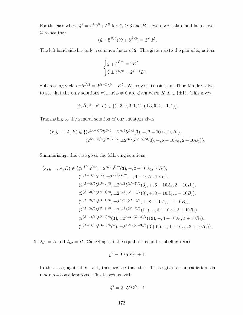
For the case where y2 = 2x1x5 + 5B for x1 ≥ 3 and B is even, we isolate and factor over
Z to see that
(y − 5B/2)(y + 5B/2) = 2x1x5.
The left hand side has only a common factor of 2. This gives rise to the pair of equationsy ∓ 5B/2 = 2K5
y ± 5B/2 = 2x1−1L5.
Subtracting yields ±5B/2 = 2x1−2L5−K5. We solve this using our Thue-Mahler solver
to see that the only solutions with KL 6= 0 are given when K,L ∈ ±1. This gives
(y, B, x1, K, L) ∈ (±3, 0, 3, 1, 1), (±3, 0, 4,−1, 1).
Translating to the general solution of our equation gives
(x, y,±, A,B) ∈ (2(A+3)/55B/5,±2A/25B/2(3),+, 2 + 10A1, 10B1),
(2(A+4)/55(B−2)/5,±2A/25(B−2)/2(3),+, 6 + 10A1, 2 + 10B1).
Summarizing, this case gives the following solutions:
(x, y,±, A,B) ∈ (2A/55B/5,±2A/25B/2(3),+, 2 + 10A1, 10B1),
(2(A+1)/55B/5,±2A/25B/2,−, 4 + 10A1, 10B1),
(2(A+4)/55(B−2)/5,±2A/25(B−2)/2(3),+, 6 + 10A1, 2 + 10B1),
(2(A+2)/55(B−1)/5,±2A/25(B−1)/2(3),+, 8 + 10A1, 1 + 10B1),
(2(A+2)/55(B−1)/5,±2A/25(B−1)/2,+, 8 + 10A1, 1 + 10B1),
(2(A+2)/55(B−3)/5,±2A/25(B−3)/2(11),+, 8 + 10A1, 3 + 10B1),
(2(A+1)/55(B−3)/5(3),±2A/25(B−3)/2(19),−, 4 + 10A1, 3 + 10B1),
(2(A+1)/55(B−3)/5(7),±2A/25(B−3)/2(3)(61),−, 4 + 10A1, 3 + 10B1).
5. 2y1 = A and 2y2 = B. Canceling out the equal terms and relabeling terms
y2 = 2x15x2x5 ± 1.
In this case, again if x1 > 1, then we see that the −1 case gives a contradiction via
modulo 4 considerations. This leaves us with
y2 = 2 · 5x2x5 − 1
172

and the positive 1 case which we defer until later. Factoring gives
(y + i)(y − i) = 2 · 5x2x5.
As the two terms on the left are coprime outside of 2, we see that
y + i = (1± i)(1± 2i)x2(a+ bi)5.
We use the Thue-Mahler equation solver on these equations and see that the only
solutions come when x2 = 0, 1 or 2 giving solutions as
(x, y, x1, x2) ∈ (0,±1, 1, 0), (1,±3, 1, 1), (1,±7, 1, 2).
These in turn give rise to solutions to the original equation of the form
(x, y,±, A,B) ∈ (2(A+1)/55B/5,±2A/25B/2,−, 4 + 10A1, 10B1),
(2(A+1)/55(B+1)/5(3),±2A/25B/2,−, 4 + 10A1, 4 + 10B1),
(2(A+1)/55(B+2)/5(7),±2A/25B/2,−, 4 + 10A1, 8 + 10B1).
Now, to handle the case where
y2 = 2x15x2x5 + 1
we first note that if x1 ≤ 2, we have that modulo 8 considerations give a contradiction.
Hence x1 ≥ 3. Factoring gives
(y + 1)(y − 1) = 2x15x2x5.
The left hand side is coprime outside of 2 and hence we have one ofy ∓ 1 = 2x1−15x2K5
y ± 1 = 2L5
y ∓ 1 = 2 · 5x2K5
y ± 1 = 2x1−1L5.
Subtracting the equations and dividing by 2 in each case gives
∓1 = 2x1−25x2K5 − L5 ∓ 1 = 5x2K5 − 2x1−2L5.
Both of these can be solved using the Thue-Mahler equation solver. The solutions with
173

KL 6= 0 are given by
(x1, x2, K, L) ∈ (3, 0, 1, 1), (3, 0,−1,−1)
in the first case and in the second case by
(x1, x2, K, L) ∈ (3, 0, 1, 1), (3, 0,−1,−1), (4, 1, 1, 1), (4, 1,−1,−1).
Converting to solutions of the original equation gives
(x, y,±, A,B) ∈ (2A/55B/5,±2A/25B/2(3),+, 2 + 10A1, 10B1),
(2(A+4)/55(B+1)/5(9),±2A/25B/2,+, 6 + 10A1, 4 + 10B1)
Collecting all the solutions in this case yields the following list:
(x, y,±, A,B) ∈ (2A/55B/5,±2A/25B/2(3),+, 2 + 10A1, 10B1),
(2(A+1)/55B/5,±2A/25B/2,−, 4 + 10A1, 10B1),
(2(A+4)/55(B+1)/5(9),±2A/25B/2,+, 6 + 10A1, 4 + 10B1),
(2(A+1)/55(B+1)/5(3),±2A/25B/2,−, 4 + 10A1, 4 + 10B1),
(2(A+1)/55(B+2)/5(7),±2A/25B/2,−, 4 + 10A1, 8 + 10B1).
6. 2y1 = A and 5x2 = B. Canceling out the equal terms and relabeling terms
5y2 y2 = 2x1x5 ± 1.
We can reduce this to exactly case (iii), which we solved using Chabauty and Elliptic
Curve Chabauty techniques, by removing the power of 5 on the left hand side by
multiplying through by 55 if y2 is odd and a suitable power of 2 which gives rise to the
equations
Y 2 = X5 ± 2A or Y 2 = X5 ± 2A55.
Here we are interested in the cases where 2 | gcd(X, Y ) and thus are left with the list
given by
(X, Y, A,±) ∈ (2,±6, 2,+), (2,±4, 4,−), (2,±8, 5,+), (6,±88, 5,−)
174

for the first equation and for the second equation,
(X, Y, A,±) ∈ (20,±2000, 8,+).
The cases where (X, Y, A,±) = (2,±8, 5,+) or (6,±88, 5,−) are inadmissible since the
power of 2 in Y 2 does not match the value of A. This leaves us only three solutions
which in terms of our original equation are given by
(x, y,±, A,B) ∈ (2A/55B/5,±2A/25B/2(3),+, 2 + 10A1, 10B1),
(2(A+1)/55B/5,±2A/25B/2,−, 4 + 10A1, 10B1),
(2(A+2)/55B/5,±2(A+12)/25(B+1)/2,+, 8 + 10A1, 5 + 10B1).
7. 5x1 = A and 2y2 = 5x2. In this case, we have
2y1 y2 = x5 ± 5B.
We can proceed similar to case 3. If y1 is even, then we look at solutions to the equation
Y 2 = X5 ± 5B
and if y1 is odd, multiply through by 25 and look at solutions to the equation
Y 2 = X5 ± 255B.
Using Chabauty and Elliptic Curve Chabauty, we have the solutions given in the case
of Y 2 = X5 ± 5B by
(X, Y, B,±) ∈ (−1, 0, 0,+), (0,±1, 0,+), (1, 0, 0,−), (−1,±2, 1,+), (0,±5, 2,+),
(0,±25, 4,+), (5,±50, 4,−), (−5, 0, 5,+),
(5, 0, 5,−), (0,±125, 6,+), (0,±625, 8,+)
and in the second case by
(X, Y, B,±) ∈ (−2, 0, 0,+), (2,±8, 0,+), (2, 0, 0,−),
(6,±88, 0,+), (−10, 0, 5,+), (10, 0, 5,−).
In the first case, there are only two solutions with non-zero entries and these are given
by
(X, Y,C,±) ∈ (−1,±2, 1,+), (5,±50, 4,−)
175

The second solution above does not satisfy 2y2 = 5x2 (it satisfies 2y2 = B). The
remaining case corresponds to the solution given by
(x, y,±, A,B) ∈ (−2A/55(B−1)/5,±2(2+A)/25(B−1)/2,+, 10A1, 1 + 10B1)
In the second case, we see that the only solutions correspond to when B = 0. These
are precisely the solutions discussed in case (ix) below and are given by
(x, y,±, A,B) ∈ (2A/55B/5(3),±2(1+A)/25B/2(11),−, 5 + 5A1, 10B1),
(2A/55B/5,±2(1+A)/25B/2,+, 5 + 5A1, 10B1).
Hence all solutions in this case are given by
(x, y,±, A,B) ∈ (−2A/55(B−1)/5,±2(2+A)/25(B−1)/2,+, 10A1, 1 + 10B1),
(2A/55B/5(3),±2(1+A)/25B/2(11),−, 5 + 5A1, 10B1),
(2A/55B/5,±2(1+A)/25B/2,+, 5 + 5A1, 10B1).
8. 5x1 = A and 2y2 = B. In this case, we have
2y1 y2 = 5x2x5 ± 1.
In the case where x2 > 0, we see that modulo 5, we must have that
y2 = ±2y1
which is a contradiction unless y1 is even. When this is even, this case gives rise to
solutions of
Y 2 = X5 ± 5C
for some constant 0 ≤ C ≤ 9. These solutions were discussed in case (vii) above
and solved by Chabauty and Elliptic Curve Chabauty techniques. There are only two
solutions with non-zero entries and these are given by
(X, Y,C,±) ∈ (−1,±2, 1,+), (5,±50, 4,−).
The case when C = 1 above does not correspond to a solution in this case as it is too
small. Hence we are given solutions only by the second case above which corresponds
to
(x, y,±, A,B) ∈ (2A/55(1+B)/5,±2(2+A)/25B/2,−, 10A1, 4 + 10B1).
176

If x2 = 0, then we see as in case (ix) below that the solutions are given by
(x, y,±, A,B) ∈ (2A/55B/5(3),±2(1+A)/25B/2(11),−, 5 + 5A1, 10B1),
(2A/55B/5,±2(1+A)/25B/2,+, 5 + 5A1, 10B1).
Hence all solutions in this case are given by
(x, y,±, A,B) ∈ (2A/55(1+B)/5,±2(2+A)/25B/2,−, 10A1, 4 + 10B1),
(2A/55B/5(3),±2(1+A)/25B/2(11),−, 5 + 5A1, 10B1),
(2A/55B/5,±2(1+A)/25B/2,+, 5 + 5A1, 10B1).
9. 5x1 = A and 5x2 = B. In this case, we have
2y15y2 y2 = x5 ± 1.
By work done by Bennett and Skinner as stated in Theorem 1.6.2, this gives rise to a
solution to
X5 + Y 5 = CZ2
with C ∈ 1, 2, 5, 10. In their work, they show that this case has no solutions when
y = ±1 except for
(X, Y, Z, C) ∈ (3,−1,±11, 2), (1,−1, 0, C), (−1, 1, 0, C), (1, 1, 1, 2).
We drop the cases where z = 0 as these have been considered already. Translating back
to the original problem, we have that
(x, y,±, A,B) = (2A/55B/5(3),±2(1+A)/25B/2(11),−, 5 + 5A1, 10B1),
(2A/55B/5,±2(1+A)/25B/2,+, 5 + 5A1, 10B1)
are the solutions that arise from this case.
We finish off with a theorem that will be used heavily later.
Theorem 3.2.11. Let d, `,m ≥ 0 be integers and let p 6= 5 be an odd prime number. Then
solutions to the equations
d2 = 2`5mp5 ± 1 d2 = ±2`p5 ± 5m d2 = ±2`5m ± p5
d2 = 2` ± 5mp5 5d2 = ±2` ± p5 5d2 = ±2`p5 ± 1
177

are given by
192 = 2 · 35 − 53 (183)2 = 2 · 75 − 53
4012 = −2 · 53 + 115 5(7)2 = 35 + 2
5(19)2 = −35 + 211.
In particular, the equations
d2 = 2`5mp5 ± 1 d2 = 2` ± 5mp5 5d2 = ±2`p5 ± 1
have no solutions.
3.3 Other Results
The following are results used from Wilfrid Ivorra [Ivo04][p.38-45]. Define
f(n) :=
18 + 2 log2 n if n < 296
435 + 10 log2 n if n ≥ 296.
Theorem 3.3.1. Solutions to d2 − 1 = 2`pn with d ≥ 1 and d, `, n ∈ Z nonnegative integers
are given by
1. n = 0 and (d, `, p) = (3, 3, p).
2. n = 1 and (d, `, p) ∈ (2, 0, 3), (5, 3, 3), (7, 4, 3), (9, 4, 5), (2p − 1, `, 2`−2 + 1), (2p +
1, `, 2`−2 − 1) with ` ≥ 5 in the last two cases.
3. n = 2 and (d, `, p) = (17, 5, 3).
Theorem 3.3.2. Solutions to d2 + 1 = 2`pn with d ≥ 1 and d, `, n ∈ Z nonnegative integers
are given by
1. n = 0 and (d, `, p) = (1, 1, p).
2. n = 1 and (d, `, p) ∈ (5, 1, 13), (d, 0, 1), (d, 1, 1).
3. n = 2 and (d, `, p) = (d, 1, p) with p ≡ 1 (mod 4) and p 6= 13.
4. n = 4 and (d, `, p) = (239, 1, 13).
Theorem 3.3.3. Solutions to d2 + 2` = pn with d ≥ 1 and d, `, n ∈ Z nonnegative integers
are given by
178

1. n = 1 and ` < log2 p.
2. n = 2 and (d, `, p) ∈ (3, 4, 5), (1, 3, 3), (p− 2, `, 2`−2 + 1) where in the last case, ` ≥ 5.
3. n = 3 and (d, `, p) ∈ (5, 1, 3), (11, 2, 5).
4. n = 4 and (d, `, p) = (7, 5, 3).
Theorem 3.3.4. Solutions to d2 − 2` = pn with d ≥ 1 and d, `, n ∈ Z nonnegative integers
are given by
1. n = 0 and ` odd.
2. n = 1 and ` < f(p).
3. n = 2 and (d, `, p) = (p+ 2, `, 2`−2 − 1) with ` ≥ 4.
4. n = 3 and (d, `, p) = (71, 7, 17).
Theorem 3.3.5. Solutions to d2 + pn = 2` with d ≥ 1 and d, `, n ∈ Z nonnegative integers
are given by
1. n = 0 and (d, `, p) = (1, 1, p).
2. n = 1 and ` < f(p).
3. n = 3 and (d, `, p) ∈ (13, 9, 7).
Theorem 3.3.6. Solutions to 2d2 + 1 = pn with d ≥ 1 and d, n ∈ Z nonnegative integers are
given by
1. n = 1.
2. n = 2.
3. n = 5 and (d, p) = (11, 3).
Theorem 3.3.7. Solutions to 2d2− 1 = pn with d ≥ 1 and d, n ∈ Z nonnegative integers are
given by
1. n = 0 and d = 1.
2. n = 1.
3. n = 2.
4. n = 3 and (d, p) = (78, 23).
This final result on Catalan’s conjecture is due to Mihailescu [Mih04].
Theorem 3.3.8. (Mihailescu’s Theorem) The only solution to the Diophantine equation
xm − yn = 1 in positive integers x, y, n,m with n,m ≥ 2 is given by 32 − 23 = 1.
179

3.4 Diophantine Equations Relating to Elliptic Curves
In this section, we solve the following Diophantine equations where d ≥ 1, `,m, n ≥ 0,
p 6= 2, 5 and we do not have (+,−) in the two ± signs:
1. d2 − 2`5mpn = ±1
2. d2 ± 2`pn = ±5m
3. d2 ± 2`5m = ±pn
4. d2 ± 2` = ±5mpn
5. 5d2 ± 2` = ±pn
6. 5d2 ± 2`pn = ±1.
This will help simplify the classification of primes such that there is an elliptic curve with
rational two torsion and conductor in the set 50p, 200p and 400p. Throughout let Pmin(n)
denote the minimum prime dividing n.
Theorem 3.4.1. Let p 6= 2, 5 be a prime number with `,m, n ≥ 0 and d ≥ 1.
1. Solutions to d2 − 2`5mpn = 1 are given by
(a) n = 0 and (d, `,m) ∈ (3, 3, 0), (9, 4, 1).
(b) n = 1 and
a) p = 3 and (d, `,m) ∈ (2, 0, 0), (5, 3, 0), (7, 4, 0), (4, 0, 1), (11, 3, 1), (49, 5, 2).b) (d, `,m, p) ∈ (2p− 1, `, 0, 2`−2 + 1), (2p+ 1, `, 0, 2`−2 − 1) with ` ≥ 5.
c) (d, `,m, p) ∈ (2`−1 + 1, `,m, 2`−2+15m
) with m ≥ 1 and ` ≥ 4 even.
d) (d, `,m, p) ∈ (p+ 1, 0,m, 5m − 2), (p− 1, 0,m, 5m + 2) with m ≥ 1.
e) (d, `,m, p) ∈ (4p− 1, 3,m, 5m+12
) with m ≥ 1.
f) (d, `,m, p) ∈ (2p− 1, `,m, 2`−25m + 1), (2p+ 1, `,m, 2`−25m − 1) with m ≥ 1
and ` ≥ 3.
g) (d, `,m, p) = (2 · 5m − 1, 4,m, 5m−14
) and m odd.
(c) n = 2 and (d, `,m, p) ∈ (17, 5, 2, 3), (19, 3, 1, 3), (99, 3, 2, 7).
(d) n = 3 and (d, `,m, p) = (26, 0, 2, 3).
(e) n = 4 and (d, `,m, p) = (161, 6, 1, 3).
(f) Pmin(n) ≥ 7, d = 2 · 5m − 1 and 4pn = 5m − 1 with m odd and ` = 4.
2. Solutions to d2 − 2`5mpn = −1 with `,m, n ≥ 0 and d ≥ 1 are given by
180

(a) m = 0 and
i. p ≥ 5 and (d, `, n) = (1, 1, 0).
ii. p = 13 and (d, `, n) ∈ (5, 1, 1), (239, 1, 4).
iii. p 6= 13, p ≡ 1 (mod 4) and (`, n) = (1, 2).
iv. (`, n) ∈ (0, 1), (1, 1)
(b) n = 0 and (d, `,m) ∈ (2, 0, 1), (3, 1, 1), (7, 1, 2).
(c) m,n ≥ 1, ` = 0, 1 and p ≡ 1 (mod 4).
1. (a) Case 1: m = 0 or n = 0. This is done in Ivorra’s thesis (see Theorem 3.3.1).
Note that the (d, `, n, p) = (9, 4, 1, 5) solution above is given as (d, `,m, n, p) =
(9, 4, 1, 0, p). Thus throughout, we assume that m > 0 and that n > 0.
Case 2: p = 3 This case was done in [Mul06] Gives the solutions
(d, `,m, n) ∈ (161, 6, 1, 4), (9, 4, 1, 0), (26, 0, 2, 3), (49, 5, 2, 1),
(4, 0, 1, 1), (19, 3, 1, 2), (11, 3, 1, 1)
and a potential solution given from 5 · 3` = 2m−2 + 1 with ` ≥ 1 and m ≥ 5. For
this case, modulo 5 shows us that 2m−2 ≡ −1 (mod 5) and so m ≡ 0 (mod 4).
Modulo 3 gives 2m−2 ≡ −1 (mod 3) and so m is odd which gives a contradiction.
Thus this last case does not occur and the other cases are listed in the statement.
Hence throughout we suppose that p ≥ 7.
Case 3: ` = 0. Here we have that d2 − 1 = 5mpn. As d is even, we have that
modulo 4, we see that p ≡ 3 (mod 4) and that n is odd. Factoring the left hand
side gives (d− 1)(d+ 1) = 5mpn which gives
d± 1 = 5m
d∓ 1 = pn
where the signs above match up3 In either case, taking the difference gives
±2 = 5m − pn.
As we have already shown that n is odd, we begin breaking this into mini cases.
3A positive sign for the first term means you must use a negative sign in the second term. This conventionwill be consistent throughout the paper, especially in this section.
181

Case 3a: n = 1. This gives p = 5m ∓ 2 and d = p ± 1 where again the signs
match up.
Case 3b: 3 | n. This gives (pn/3)3 = 5m ∓ 2. If m is even, then looking at
this as an integer solution to an elliptic curve of the form y2 = x3 ± 2. We
use Theorem 3.1.4 to show that this has no solution for x prime when we have
y2 = x3 + 2 and Theorem 3.1.8 to see when y2 = x3 − 2 that the solutions are
given by (x, y) = (3,±5) (a solution we have already found). Now, assume that
m is odd. Since we know that p ≥ 7 a quick check locally at 3 shows that
(pn/3)3 = 5m ∓ 2 ≡ 2∓ 2 (mod 3)
so pn ≡ 0 (mod 3) or pn ≡ 1 (mod 3). The first case gives p = 3, a case we have
already considered above, and so we must have that (pn/3)3 = 5m + 2 with m
odd. Multiplying by 53 gives (5pn/3)3 = (5(m+3)/2)2 + 2 · 53, that is, a solution to
y2 = x3 − 250. A check with Theorem 3.1.8 shows that there are no 2, 5,∞solutions.
Case 3c: Pmin(n) ≥ 5. This gives pn = 5m ∓ 2. If we think of this as a solution
(x, y, z) = (1,∓1, p) to 5mxn + 2yn = zn for a prime n ≥ 3, then we can use
Theorem 1.6.1 to show that we have no solutions.
Case 4: ` = 1. Here we have locally at 8 that
d2 ≡ 1 + 2`5mpn ≡
3 (mod 8) if either n is even or p ≡ 1, 5 (mod 8)
7 (mod 8) if n is odd and p ≡ 3, 7 (mod 8)
holding since 2 · 5m ≡ 2 (mod 8) always. This is a contradiction since odd squares
modulo 8 are congruent to 1.
Case 5: ` = 2. If ` = 2, then notice that 4 · 5m ≡ 4 (mod 8) and that 4pn ≡4 (mod 8). Hence we have that 1 + 2l5mpn ≡ 5 (mod 8) always, a contradiction.
Case 6: ` ≥ 6, Pmin(n) ≥ 7. If ` ≥ 6, then using Theorem 1.6.4, we see that
there are no solutions in this case.
Case 7: 3 | n. Here, we have the equation d2 = 2`5m(pn/3)3+1. Let ` = 3L+λ and
m = 3M + µ where λ, µ ∈ 0, 1, 2 and L,M are nonnegative integers. Rewriting
the equation gives
d2 = 2λ5µ(2L5Mpn/3)3 + 1.
182

Multiplying through by 22λ and 52µ gives
(2λ5µd)2 = (2L+λ5M+µpn/3)3 + 22λ52µ
Thus it suffices to look up all 2, 5,∞-integer points on elliptic curves with the
above form. This is done in Section 3.1. A quick check on the tables shows that
the only entry that has an x-coordinate of the form x = 2L+λ5M+µpn/3 and the
constant term of the form 22λ52µ corresponds to the solution
(25 · 26)2 = (25 · 3)3 + 20 · 54.
This corresponds to
(d, `,m, n, p) = (26, 0, 2, 3, 3)
which is a solution we already have found since p = 3.
Case 8: 5 | n. Checking with Theorem 3.2.11, we see that this case gives no
solutions.
Case 9: ` ≥ 3, m,n ≥ 1 and one of 2 | n or ` = 3, 4, 5 with Pmin(n) ≥ 7 or
n = 1. We rearrange the equation to d2 − 1 = 2`5mpn and factor the left hand
side to see that
(d− 1)(d+ 1) = d2 − 1 = 2`5mpn.
This leads to the following possible situations
d∓ 1 = 2`−1
d± 1 = 2 · 5mpn
d∓ 1 = 2`−1pn
d± 1 = 2 · 5m
d∓ 1 = 2`−15m
d± 1 = 2 · pn
d∓ 1 = 2`−15mpn
d± 1 = 2.
The last case has no such solutions as m and p are positive. Eliminating d in each
of the first 3 cases gives the equations
i. ±1 = 5mpn − 2`−2.
ii. ±1 = 5m − 2`−2pn.
iii. ±1 = pn − 2`−25m.
Now we divide into subcases
Case 9a: n is even.
i. For this case, rewrite the equation as 2`−2 ± 1 = 5m(pn/2)2. Using Theorem
1.6.2, we get a contradiction when ` ≥ 6. Hence, we have that ` = 3, 4, 5.
183

In these cases, the only solution with n ≥ 2 even is given by (p, `,m, d, n) =
(3, 5, 0, 17, 2).
ii. For this case, rewrite the equation as 2`−2pn = 5m ∓ 1 which gives a solution
to the equation Cz2 = xm + ym where C ∈ 1, 2 (possible grouping extra
powers of 2 inside z). Theorem 1.6.2 implies that m < 4. Since m > 0, and n
is even, a quick check of the 3 possible values of n shows that we have n = 1
in all admissible cases, contradicting this case.
iii. For this case, if pn = 2`−25m − 1, then if ` − 2 ≥ 3, we have that pn ≡−1 (mod 8), a contradiction since n is even. If ` = 4, then we get that
pn ≡ 3 (mod 8) which is also a contradiction. This leaves the case when
` = 3. In this case, a result of Cohn [Coh96] shows us that we have no
solutions when m > 2. For m ≤ 2, we get solutions given by
(d, `,m, n, p) ∈ (19, 3, 1, 2, 3), (99, 3, 2, 2, 7).
Now, if pn = 2`−25m + 1, we move the 1 to the other side and factor to see
that
(pn/2 − 1)(pn/2 + 1) = 2`−25m.
Since the greatest common divisor on the left is 2, we see that when ` = 3 we
have a contradiction. Thus ` ≥ 4 and further, we are in one of the following
cases pn/2 ∓ 1 = 2 · 5m
pn/2 ± 1 = 2`−3
pn/2 − 1 = 2
pn/2 + 1 = 2`−35m.
In the second case, it is clear that the only solution comes when (d, `,m, n, p) =
(17, 5, 0, 2, 3). In the first case, eliminating the p factor gives 5m − 2`−4 = ±1
and Mihailescu’s Theorem (Theorem 3.3.8) implies that either m = 1 and
` = 6 or that m = 0 and ` = 5. In these cases, we have the solutions given by
(d, `,m, n, p) ∈ (161, 6, 1, 4, 3), (17, 5, 0, 2, 3).
Case 9b: ` = 3, 4, 5 and Pmin(n) ≥ 7.
i. For this case, plugging in ` = 3, 4, 5 immediately shows that there are no
solutions with n ≥ 3.
ii. In this case, notice that ±1 = 5m − 2pn can be handled by Theorem 1.6.1 to
show that the only solution to this equation is given by −1 = 50− 2p0. When
` = 4 or 5, if −1 = 5m − 2`pn, then we have modulo 4 that −1 ≡ 1 (mod 4)
184
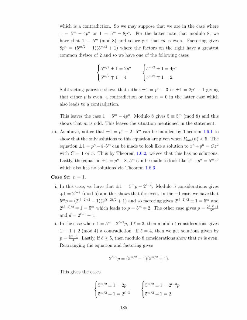
which is a contradiction. So we may suppose that we are in the case where
1 = 5m − 4pn or 1 = 5m − 8pn. For the latter note that modulo 8, we
have that 1 ≡ 5m (mod 8) and so we get that m is even. Factoring gives
8pn = (5m/2 − 1)(5m/2 + 1) where the factors on the right have a greatest
common divisor of 2 and so we have one of the following cases5m/2 ± 1 = 2pn
5m/2 ∓ 1 = 4
5m/2 ± 1 = 4pn
5m/2 ∓ 1 = 2.
Subtracting pairwise shows that either ±1 = pn − 3 or ±1 = 2pn − 1 giving
that either p is even, a contradiction or that n = 0 in the latter case which
also leads to a contradiction.
This leaves the case 1 = 5m − 4pn. Modulo 8 gives 5 ≡ 5m (mod 8) and this
shows that m is odd. This leaves the situation mentioned in the statement.
iii. As above, notice that ±1 = pn − 2 · 5m can be handled by Theorem 1.6.1 to
show that the only solutions to this equation are given when Pmin(n) < 5. The
equation ±1 = pn−4 ·5m can be made to look like a solution to xn+yn = Cz2
with C = 1 or 5. Thus by Theorem 1.6.2, we see that this has no solutions.
Lastly, the equation ±1 = pn−8 ·5m can be made to look like xn +yn = 5mz3
which also has no solutions via Theorem 1.6.6.
Case 9c: n = 1.
i. In this case, we have that ±1 = 5mp − 2`−2. Modulo 5 considerations gives
∓1 = 2`−2 (mod 5) and this shows that ` is even. In the −1 case, we have that
5mp = (2(`−2)/2 − 1)(2(`−2)/2 + 1) and so factoring gives 2(`−2)/2 ± 1 = 5m and
2(`−2)/2 ∓ 1 = 5m which leads to p = 5m ∓ 2. The other case gives p = 2`−2+15m
and d = 2`−1 + 1.
ii. In the case where 1 = 5m−2`−2p, if ` = 3, then modulo 4 considerations gives
1 ≡ 1 + 2 (mod 4) a contradiction. If ` = 4, then we get solutions given by
p = 5m−14
. Lastly, if ` ≥ 5, then modulo 8 considerations show that m is even.
Rearranging the equation and factoring gives
2`−2p = (5m/2 − 1)(5m/2 + 1).
This gives the cases5m/2 ± 1 = 2p
5m/2 ∓ 1 = 2`−3
5m/2 ± 1 = 2`−3p
5m/2 ∓ 1 = 2.
185
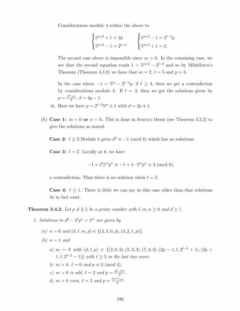
Considerations modulo 4 reduce the above to5m/2 + 1 = 2p
5m/2 − 1 = 2`−3
5m/2 − 1 = 2`−3p
5m/2 + 1 = 2.
The second case above is impossible since m > 0. In the remaining case, we
see that the second equation reads 1 = 5m/2 − 2`−3 and so by Mihailescu’s
Theorem (Theorem 3.3.8) we have that m = 2, ` = 5 and p = 3.
In the case where −1 = 5m − 2`−2p, if ` ≥ 4, then we get a contradiction
by considerations modulo 4. If ` = 3, then we get the solutions given by
p = 5m+12
, d = 4p− 1.
iii. Here we have p = 2`−25m ± 1 with d = 2p∓ 1.
(b) Case 1: m = 0 or n = 0. This is done in Ivorra’s thesis (see Theorem 3.3.2) to
give the solutions as stated.
Case 2: ` ≥ 3 Modulo 8 gives d2 ≡ −1 (mod 8) which has no solutions.
Case 3: ` = 2. Locally at 8, we have
−1 + 2`5mpn ≡ −1 + 4 · 5mpn ≡ 3 (mod 8),
a contradiction. Thus there is no solution when ` = 2.
Case 4: ` ≤ 1. There is little we can say in this case other than that solutions
do in fact exist.
Theorem 3.4.2. Let p 6= 2, 5 be a prime number with `,m, n ≥ 0 and d ≥ 1.
1. Solutions to d2 − 2`pn = 5m are given by
(a) n = 0 and (d, `,m, p) ∈ (3, 3, 0, p), (3, 2, 1, p).
(b) n = 1 and
a) m = 0 with (d, `, p) ∈ (2, 0, 3), (5, 3, 3), (7, 4, 3), (2p − 1, `, 2`−2 + 1), (2p +
1, `, 2`−2 − 1) with ` ≥ 5 in the last two cases.
b) m > 0, ` = 0 and p ≡ 3 (mod 4).
c) m > 0 is odd, ` = 2 and p = d2−5m
4.
d) m > 0 even, ` = 3 and p = 5m/2+12
.
186

e) m > 0 even, ` ≥ 3 and p = 2`−2± 5m/2 with d = 2`−1± 5m/2 and both signs the
same.
(c) n = 2 and
i. (d, `,m, p) = (5m+12, 2,m, 5m−1
4) and m is odd.
ii. (d, `,m, p) ∈ (17, 5, 0, 3).
(d) 2 ‖ n and 4pn/2 = 5m − 1 with m odd, ` = 2 and either n = 2 or Pmin(n/2) ≥ 7.
(e) n = 3 and (d, `,m, p) ∈ (29, 3, 4, 3), (59, 7, 2, 3), (73, 2, 1, 11).
(f) n = 4 and (d, `,m, p) = (129, 4, 3, 11).
(g) Pmin(n) ≥ 7, m ≥ 1 and
a ` = 0 with p ≡ 3 (mod 4).
b ` = 2 with pn = d2−5m
4and m odd.
c ` = 3 with pn = 5m/2+12
and m even.
d ` ∈ 4, 5 with pn = 2`−2 ± 5m/2 and m even.
2. Solutions to d2 + 2`pn = 5m are given by
(a) n = 0 and (d, `,m, p) ∈ (11, 2, 3, p), (3, 4, 2, p).
(b) n = 1 and
a) (d, `,m, p) = (23, 5, 4, 3).
b) p = 5m − d2 and ` = 0.
c) p = 5m−d24
and ` = 2.
d) (d, `,m, p) = (±(5m/2 − 2`−1), `,m, 5m/2 − 2`−2) ` ≥ 3 and m ≥ 2 even.
e) p = 5m/2−14
, d = 5m/2 − 2 and ` = 4 with m ≥ 2 even.
(c) n ≥ 2 is even and ` = 0 with m even and pn = 2 · 5m/2 − 1.
(d) n ≥ 2 is even and ` ∈ 0, 2 with m odd.
(e) n = 2 and (d, `,m, p) = (117, 4, 6, 11).
(f) Pmin(n) ≥ 7 and 0 ≤ ` ≤ 5 and m ≥ 1.
3. Solutions to d2 + 5m = 2`pn are
(a) n = 0 and (d, `,m, p) = (1, 1, 0, p).
(b) n = 1, ` = 0 and p ≡ 1 (mod 4).
(c) n = 1 and ` = 1.
(d) n = 2, ` = 0, p = 5m+12
, d = p− 1.
187

(e) n = 2, ` = 1 and m = 0 with p ≡ 1 (mod 4) and p 6= 13.
(f) n = 3 and (d, `,m, p) ∈ (7, 1, 1, 3), (99, 1, 2, 17).
(g) n = 4 and (d, `,m, p) = (239, 1, 0, 13).
(h) n = 5 and (d, `,m, p) ∈ (19, 1, 3, 3), (183, 1, 3, 7).
Proof. 1. Case 1: n = 0 or m = 0. This is done in Ivorra’s thesis. If n = 0, we look
up Theorem 3.3.4 for solutions to d2 − 2` = 5m. This gives solutions when m = 0 or
m = 1. When m = 0, we use Mihailescu’s Theorem (Theorem 3.3.8) to get the only
solution of (d, `,m) = (3, 3, 0). When m = 1, we see that ` must be even via modulo 5
considerations and so the left hand side factors to give the equationsd− 2`/2 = 1
d+ 2`/2 = 5.
Subtracting these two equations gives 2`/2+1 = 4 and so ` = 2. This gives another
solution given by (d, `,m) = (3, 2, 1).
When m = 0 and n > 0, via Theorem 3.3.1 (recalling that p 6= 5), we get the solutions
mentioned in the theorem. For the duration of this proof, we suppose that m,n > 0.
Case 2: 3 | n. If ` ≡ 0 (mod 3) then (x, y) = (2`/3pn/3, d) is a solution to y2 = x3 +5m.
Using Theorem 3.1.2, we have that the only solution of this shape that arises is when
(x, y) = (6,±29) and this gives (d, `,m, n, p) = (29, 3, 4, 3, 3).
If ` ≡ 1 (mod 3) then (x, y) = (2(`+2)/3pn/3, 2d) is a solution to y2 = x3 + 225m.
Using Theorem 3.1.2, we have that the only solution of this shape that arises is when
(x, y) = (24,±118) and this gives (d, `,m, n, p) = (59, 7, 2, 3, 3).
If ` ≡ 2 (mod 3) then (x, y) = (2(`+4)/3pn/3, 4d) is a solution to y2 = x3 + 245m.
Using Theorem 3.1.2, we have that the only solution of this shape that arises is when
(x, y) = (44,±292) and this gives (d, `,m, n, p) = (73, 2, 1, 3, 11).
Case 3: 5 | n. Checking with Theorem 3.2.11, we see that this case gives no solutions.
Case 4: Pmin(n) ≥ 7 and ` ≥ 6. Using the modular method of Theorem 1.6.5, we can
show that this equation has no solutions.
Case 5: n even. We break this into subcases.
188

Case 5a: ` = 0. In this case, we have d2 − pn = 5m. Notice that d must be even since
p is odd and so considerations modulo 4 give −1 ≡ 1 (mod 4), a contradiction.
Case 5b: ` = 1. In this case, we have d2 − 2pn = 5m. Considerations modulo 5 give
d2 ≡ 2pn (mod 5). Since n is even, we know that 2 must be a square modulo 5, a
contradiction.
Case 5c: ` = 2. Local considerations at 8 give us that
d2 = 2`pn + 5m ≡ 4 + 5m (mod 8)
and this value is either 1 or 5 depending on if m is odd or even. If m is even, then we
get d2 ≡ 5 (mod 8) which is a contradiction. Hence m is odd. Thus, let m = 2k + 1
and j = n/2. Factoring gives
5m = d2 − 4p2j = (d− 2pj)(d+ 2pj).
As gcd(d− 2pj, d+ 2pj) = 1, we have that
d+ 2pj = 5m
d− 2pj = 1.
Subtracting these two equations gives 4pj = 5m − 1. If 4 | n, then j is also even and
hence the above gives rise to a solution to z2 = xm + ym. By Theorem 1.6.2, we know
that this implies that m < 4. Checking values of m = 1 and m = 3 shows that m = 3
gives rise to p = 31 and j = 1 contradicting that j was even.
If 2 ‖ n, then we get 4pn/2 = 5m − 1. Modulo 8 considerations shows that m is odd.
Case 5d: ` ≥ 3. Local considerations at 8 give us that
1 ≡ d2 = 2`pn + 5m ≡ 5m (mod 8)
and so, we see that m must be even. Now, considerations at 3 show us that
d2 = 2`pn + 5m ≡ 2` + 1 (mod 3).
Thus, ` has to be odd (as 2 is a quadratic non-residue modulo 3). Next, modulo 5 gives
d2 = 2`pn ≡ 2 · (2(`−1)/2pn/2)2 (mod 5)
189

and so once again, we see that 2 is a square modulo 5 which is a contradiction.
Case 6: n = 1 or Pmin(n) ≥ 7. When ` = 0, d is even and so modulo 4 considerations
show that p ≡ 3 (mod 4). When ` = 1, we see that d2 − 2pn = 5m. Reducing modulo
4 yields that d2 ≡ 3 (mod 4) and this is a contradiction. When ` = 2, then we have
d2 = 5m + 4pn ≡ 5m + 4 (mod 8) showing that m is odd since 5 is not a square modulo
8. Lastly, if ` ≥ 3, then m is even by reducing modulo 8 and thus we can factor giving
(d− 5m/2)(d+ 5m/2) = 2`pn. This gives the following casesd− 5m/2 = 2
d+ 5m/2 = 2`−1pn
d∓ 5m/2 = 2pn
d± 5m/2 = 2`−1.
In the first case, eliminating d yields 5m/2 = 2`−2pn − 1. When ` = 3, This gives
pn = 5m/2+12
which is a potential solution. When ` ≥ 4, modulo 4 considerations give a
contradiction. In the second case, eliminating gives ±5m/2 = 2`−2− pn. The case when
` = 3 is solved via Theorem 1.6.1 and the other cases are included in the theorem.
2. Case 1: m = 0 or n = 0 If m = 0 then we immediately see we have no solution since
d is positive. If n = 0, then from Ivorra’s thesis (see Theorem 3.3.3), we see that the
only solutions are given by
(d, `,m) ∈ (3, 4, 2), (11, 2, 3).
From now on, assume that m > 0 and n > 0.
Case 2: 3 | n
If ` ≡ 0 (mod 3) then (x, y) = (−2`/3pn/3, d) is a solution to y2 = x3 + 5m.
If ` ≡ 1 (mod 3) then (x, y) = (−2(`+2)/3pn/3, 2d) is a solution to y2 = x3 + 225m.
If ` ≡ 2 (mod 3) then (x, y) = (−2(`+4)/3pn/3, 4d) is a solution to y2 = x3 + 245m.
Using Theorem 3.1.2, we see that all the solutions which have a negative x-coordinate
are not integer solutions (there is one 2, 5,∞-integer solution with constant term
22+6n · 53 but this does not translate to a solution) and so these cases do not give a
solution.
Case 3: 5 | n. Checking with Theorem 3.2.11, we see that this case gives no solutions.
190
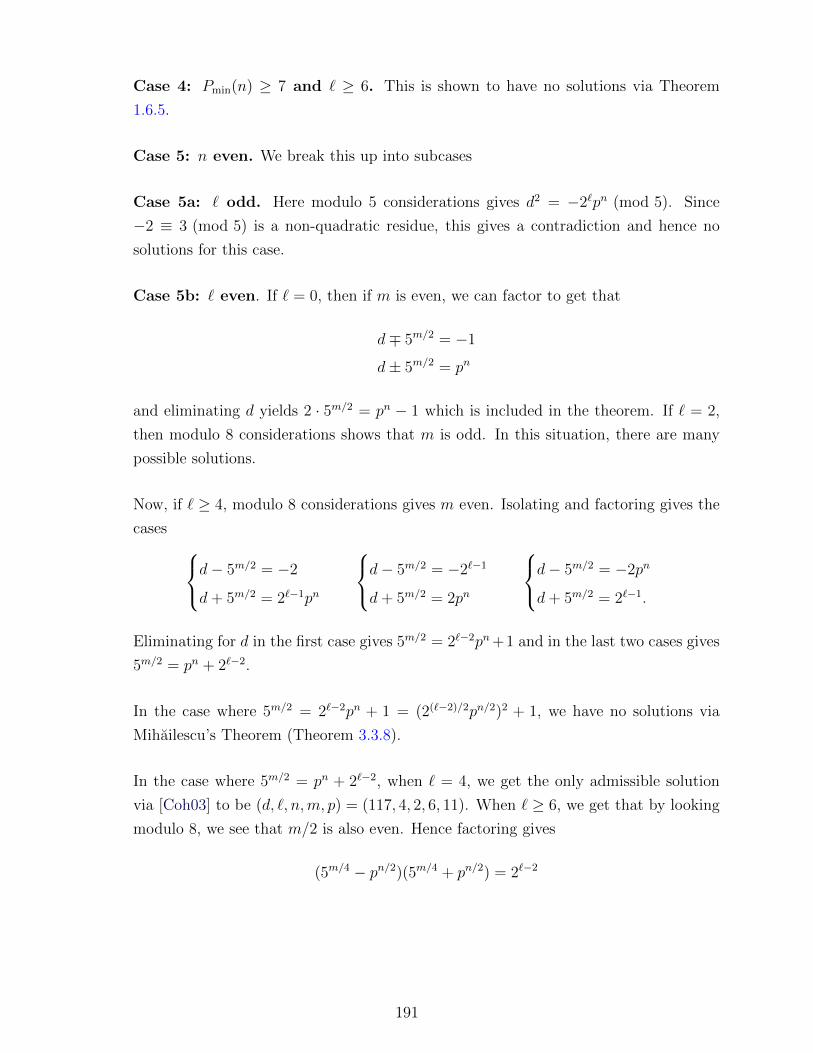
Case 4: Pmin(n) ≥ 7 and ` ≥ 6. This is shown to have no solutions via Theorem
1.6.5.
Case 5: n even. We break this up into subcases
Case 5a: ` odd. Here modulo 5 considerations gives d2 = −2`pn (mod 5). Since
−2 ≡ 3 (mod 5) is a non-quadratic residue, this gives a contradiction and hence no
solutions for this case.
Case 5b: ` even. If ` = 0, then if m is even, we can factor to get that
d∓ 5m/2 = −1
d± 5m/2 = pn
and eliminating d yields 2 · 5m/2 = pn − 1 which is included in the theorem. If ` = 2,
then modulo 8 considerations shows that m is odd. In this situation, there are many
possible solutions.
Now, if ` ≥ 4, modulo 8 considerations gives m even. Isolating and factoring gives the
cases d− 5m/2 = −2
d+ 5m/2 = 2`−1pn
d− 5m/2 = −2`−1
d+ 5m/2 = 2pn
d− 5m/2 = −2pn
d+ 5m/2 = 2`−1.
Eliminating for d in the first case gives 5m/2 = 2`−2pn+1 and in the last two cases gives
5m/2 = pn + 2`−2.
In the case where 5m/2 = 2`−2pn + 1 = (2(`−2)/2pn/2)2 + 1, we have no solutions via
Mihailescu’s Theorem (Theorem 3.3.8).
In the case where 5m/2 = pn + 2`−2, when ` = 4, we get the only admissible solution
via [Coh03] to be (d, `, n,m, p) = (117, 4, 2, 6, 11). When ` ≥ 6, we get that by looking
modulo 8, we see that m/2 is also even. Hence factoring gives
(5m/4 − pn/2)(5m/4 + pn/2) = 2`−2
191

which in turn gives the cases 5m/4 − pn/2 = 2
5m/4 + pn/2 = 2`−3.
Eliminating for p gives 5m/4 = 2`−4 − 1 and so 1 = 2`−4 − 5m/4. Mihailescu’s Theorem
(Theorem 3.3.8) implies that `− 4 = 0 (since ` is even) and this gives a contradiction.
Thus there are no solutions in this case.
Case 6: n = 1. If ` = 0, then we can only say p = 5m − d2. If ` = 1 then modulo
4 considerations gives d2 ≡ 5m − 2p ≡ 1 − 2 ≡ −1 (mod 4) which is a contradiction.
When ` = 2, then we can only say that d2 = 5m − 4p. When ` ≥ 3, modulo 8
considerations show that m is even. Just as in the case 5b above, we can factor to give
(d− 5m/2)(d+ 5m/2) = 2`p leading tod− 5m/2 = −2
d+ 5m/2 = 2`−1p
d− 5m/2 = −2`−1
d+ 5m/2 = 2p
d− 5m/2 = −2p
d+ 5m/2 = 2`−1.
Eliminating for d in the first case gives 5m/2 = 2`−2p + 1 and in the last two cases
gives 5m/2 = p + 2`−2. The second case gives p = 5m/2 − 2`−2. The first case needs to
be broken into more cases. When ` = 3, we get a contradiction by looking modulo 4.
When ` = 4, we get p = 5m/2−14
and we can say nothing more. When ` ≥ 5, modulo
8 considerations give m/2 is even and so factoring gives (5m/4 − 1)(5m/4 + 1) = 2`−2p.
This leads to 5m/4 ∓ 1 = 2p
5m/4 ± 1 = 2`−3.
Looking at the second equation, Mihailescu’s Theorem (Theorem 3.3.8) implies that of
the equations
5m/4 + 1 = 2`−3
5m/4 − 1 = 2`−3
only the second admits a solution given by m = 4 and ` = 5. This gives p = 3 in the
first equation and thus the solution given by
(d, `, n,m, p) = (23, 5, 1, 4, 3).
This completes this case.
192

3. Case 1: m = 0 or n = 0 If m = 0, then Theorem 3.3.2 shows that either (d, `, n, p) =
(1, 1, 0, p), p = 13 and (d, `, n) ∈ (5, 1, 1), (239, 1, 4) or that p ≡ 1 (mod 4), p 6= 13
and (`, n) ∈ (0, 1), (1, 1), (1, 2).
If n = 0 and m > 0, then a check with Theorem 3.3.5 shows that m = 1 and ` <
435 + 10 log2(5) ≤ 500. Checking with MAGMA for squares of the form 2` − 5 quickly
yields no results for ` ∈ 1, 2, ..., 500 (we could also refer to [Coh03] to see this has no
solutions). Thus, throughout suppose that n > 0 and m > 0.
Case 2: ` ≥ 3
Here, we have
d2 = −5m + 2lpn ≡
−5 (mod 8) if m ≡ 1 (mod 2)
−1 (mod 8) if m ≡ 0 (mod 2)
which is a contradiction since −1 and −5 are not squares modulo 8.
Case 3: ` = 2
If ` = 2, then
d2 = −5m + 2lpn ≡
−5 (mod 8) if m ≡ 1 (mod 2)
−1 (mod 8) if m ≡ 0 (mod 2)+
4p (mod 8) if n ≡ 1 (mod 2)
4 (mod 8) if n ≡ 0 (mod 2)
≡
−1 (mod 8) if m ≡ 1 (mod 2)
3 (mod 8) if m ≡ 0 (mod 2).
Since 4p ≡ 4 (mod 8) for any odd prime. Again we have a contradiction since neither
−1 nor 3 are squares modulo 8.
Case 4: ` = 1
When n ≥ 3, the solutions are given by theorems 1 and 3 of [AMLST09] (valid since
gcd(d, p) = 1 resulting from p 6= 5) to be
(d, `,m, n, p) ∈ (7, 1, 1, 3, 3), (99, 1, 2, 3, 17), (239, 1, 0, 4, 13), (19, 1, 3, 5, 3), (183, 1, 3, 5, 7).
If n = 2, then since m > 0, we have that modulo 5 considerations give d2 ≡ 2p2 (mod 5)
which is a contradiction since 2 is a quadratic non-residue.
193

If ` = 1 and n = 1, there are many solutions. If ` = 1 and n = 0, then the equation
becomes d2 + 5m = 2 which only has the solution d = 1 and m = 0.
Case 5: ` = 0
When ` = 0, the solutions are given by theorem 1 of [PR11] when n ≥ 3 and there are
no such solutions. When n = 2, we have 5m = p2− d2 = (p− d)(p+ d). Since d is even,
we know that gcd(p− d, p+ d) = gcd(p− d, 2p) = 1 and so this gives the equationsp− d = 1
p+ d = 5m
and hence p = 5m+12
, a case included in the theorem. When n = 1, this gives p = d2+5m.
Hence d is even and so p ≡ 1 (mod 4).
Theorem 3.4.3. Let p 6= 2, 5 be a prime number with `,m, n ≥ 0 and d ≥ 1.
1. Solutions to d2 − 2`5m = pn are given by
(a) n = 0 and (d, `,m) ∈ (3, 3, 0), (9, 4, 1).
(b) n = 1, m = 0 and ` < 435 + 10 log2(p).
(c) n = 1 and m > 0.
(d) n = 2 and
a) (d, `, p) = (p+ 2, `, 2`−2 − 1) with ` ≥ 4.
b) p = 2`−2 − 5m, d = 2`−1 − p and ` ≥ 3.
c) p = 5m − 2`−2, d = 2`−1 + p and ` ≥ 3.
d) p = 2`−2 · 5m − 1, d = p+ 2 and ` ≥ 3.
e) (d, `,m, p) = (13, 5, 1, 3).
(e) 2 ‖ n, m is odd, ` = 4 and p satisfies pn/2 = 5m − 4.
(f) n = 3 and (d, `,m, p) ∈ (299, 12, 1, 41), (71, 7, 0, 17), (411, 5, 5, 41).
(g) n = 4 and (d, `,m, p) ∈ (41, 6, 2, 3), (11, 3, 1, 3), (51, 3, 2, 7), (129, 4, 3, 11).
(h) n = 6 and (d, `,m, p) = (37, 7, 1, 3).
(i) Pmin(n) ≥ 7 and 0 ≤ ` ≤ 5 and m ≥ 1.
2. Solutions to d2 + pn = 2`5m are given by
194

(a) n = 0 and (d, `,m, p) ∈ (1, 1, 0, p), (13, 9, 3, 7).
(b) n = 1.
(c) 2 | n and ` = 0, 1.
(d) n = 3 and (d, `,m, p) ∈ (47, 8, 3, 31), (17, 9, 0, 7).
(e) Pmin(n) ≥ 7 and 0 ≤ ` ≤ 5 and m ≥ 1.
3. Solutions to d2 + 2`5m = pn are given by
(a) n = 1 so p = d2 + 2`5m.
(b) n = 2 and
a) (d, `,m, p) = (p− 1, 0,m, 5m+12
).
b) (d, `,m, p) = (±(p− 2`−1), `,m, 5m + 2`−2) and ` ≥ 3.
c) (d, `,m, p) = (p− 2, `,m, 2`−2 · 5m + 1) and ` ≥ 3.
(c) n = 3 and (d, `,m, p) ∈ (9, 1, 4, 11), (261, 5, 2, 41).
(d) n = 4 and (d, `,m, p) = (1, 4, 1, 3).
(e) n = 5 and (d, `,m, p) = (401, 1, 3, 11).
(f) n = 6 and (d, `,m, p) = (23, 3, 2, 3).
(g) n = 8 and (d, `,m, p) = (79, 6, 1, 3).
Proof. 1. Case 1: m = 0 or n = 0. When m = 0, we have via Theorem 3.3.4 that
(a) n = 0.
(b) n = 1 and ` < f(p) < 435 + 10 log2(p).
(c) n = 2 and (d, `, p) = (p+ 2, `, 2`−2 − 1) with ` ≥ 4.
(d) n = 3 and (d, `, p) = (71, 7, 17).
If both m = 0 and n = 0, then Mihailescu’s Theorem (Theorem 3.3.8) implies that
` = 3 and d = 3 is the only solution to d2 − 2` = 1.
If only n = 0, then we get two solutions via Theorem 3.3.1, namely
(d, `,m) ∈ (3, 3, 0), (9, 4, 1)
and the first one is discussed above. Thus throughout, suppose that m,n > 0.
195

Case 2: 3 | n. Our equation is set up in the form d2 = (pn/3)3 + 2`5m. Thus we
want solutions to y2 = x3 + 2α5β with the x coordinate a positive prime. A check on
Theorem 3.1.4 reveals that these solutions are given by
(d, `,m, n, p) ∈ (299, 12, 1, 3, 41), (71, 7, 0, 3, 17), (37, 7, 1, 6, 3), (411, 5, 5, 3, 41).
Case 3: 5 | n. Checking with Theorem 3.2.11, we see that this case gives no solutions.
Case 4: Pmin(n) ≥ 7 and ` ≥ 6. Using the modular method of Theorem 1.6.5, we can
show that this equation has no solutions.
Case 5: n is even. Suppose n is even, so n = 2k. Then if ` = 0, we have
d2 = p2k + 5m ≡ 1 +
5 if m ≡ 1 (mod 2)
1 if m ≡ 0 (mod 2)(mod 8)
≡
6 if m ≡ 1 (mod 2)
2 if m ≡ 0 (mod 2)(mod 8)
which is a contradiction since neither are squares modulo 8. If ` = 1, we have
d2 = p2k + 2 · 5m ≡ 1 + 2 ≡ 3 (mod 8)
which is a contradiction since 3 is not a square modulo 8. If ` = 2, we have
d2 = p2k + 4 · 5m ≡ 1 + 4 ≡ 5 (mod 8)
which is a contradiction since 5 is not a square modulo 8. So hence we can assume that
` ≥ 3. Factoring gives
(d+ pk)(d− pk) = 2`5m.
Since gcd(d+ pk, d− pk) = gcd(d− pk, 2d) = 2, we have thatd− pk = 2
d+ pk = 2`−15m
d± pk = 2 · 5m
d∓ pk = 2`−1
where in the first case, we do not have the d+ pk = 2 case because this least to k = 0
and d = 1 which does not yield a solution.
Now in the first case, eliminating for d yields 2`−25m = pk + 1. Using the modularity
method of Theorem 1.6.2 (where we think of 2`−25m = Cz2), we can see that k ≤ 3.
196

The cases when k = 0 or 3 were solved already and so k = 1 or k = 2.
If k = 2, then ` = 3 since otherwise modulo 8 considerations give a contradiction (` = 4
gives 3 is a square modulo 8 while ` ≥ 5 shows that −1 is a square modulo 8; both
are contradictions). Now, rewriting the equation gives −1 = p2 − 2 · 5m which has no
solutions when m > 2 by [Coh96]. When m = 1 or 2, we see that the only possible
solutions come when (d, `,m, n, p) = (11, 3, 1, 4, 3) or (d, `,m, n, p) = (51, 3, 2, 4, 7). If
k = 1, we get p = 2`−25m − 1.
In the second case, we eliminate for d yielding 5m ∓ pk = 2`−2. We break this into
subcases.
Case 5a: ` ≥ 6. By the previous cases, we know that k is a power of 2 since no other
primes divide n. Hence, considerations modulo 8 yield
pk = ∓(2`−2 − 5m) ≡ ±5m (mod 8).
Giving a contradiction unless m is even and the equation is 5m − pk = 2`−2. In this
case, we factor the left hand side and see that
(5m/2 − pk/2)(5m/2 + pk/2) = 2`−2.
As gcd(5m/2 − pk/2, 5m/2 + pk/2) = gcd(5m/2 − pk/2, 2 · 5m/2) = 2, we must have that5m/2 + pk/2 = 2`−3
5m/2 − pk/2 = 2.
Eliminating pk/2 in the above yields 5m/2−2`−4 = 1 and Mihailescu’s Theorem (Theorem
3.3.8) says that the only solutions are when m = 2 and ` = 6 giving (d, `,m, n, p) =
(41, 6, 2, 4, 3).
Case 5b: ` ≤ 5. In the case of 5m + pk = 2`−2, a quick inspection gives us that
the only solution is when ` = 5 with m = k = 1 and p = 3. This gives the solution
(d, `,m, n, p) = (13, 5, 1, 2, 3). In the case of 5m − pk = 2`−2, if ` = 3, then Theorem
1.6.1 shows that only 2 and 3 can divide 5. We have already considered the case when
3 | k and so we suppose that k is even. Then modulo 5 considerations give us that
−pk ≡ 2 (mod 5) which is a contradiction since −2 is not a quadratic residue modulo
5. If ` = 5 then Theorem 1.6.7 tells us that only 2, 3 or 5 may divide k. Since we
have considered the case when 3, 5 | k, we may suppose that k is even and the same
argument as above gives a contradiction.
197

If ` = 4 and k is even, the solutions to x2 + C = yn with C = 2, 4, or 8 are given by
[Coh03, Section 5] to be (x, y, n, C) = (5, 3, 3, 2), (2, 2, 3, 4) and (11, 5, 3, 4) (this offers
an alternative proof to the above). For our purposes, we require that y is a power of 5
and so only the last solution is admissible in our setting.
Now, suppose k is odd. Thus looking modulo 4 tells us that p ≡ 1 (mod 4). If m is
even, then factoring 5m − pk = 4 gives (5m/2 − 2)(5m/2 + 2) = pn/2 and so 5m/2 − 2 = 1
which is a contradiction. Hence m is odd.
2. Case 1: m = 0 or n = 0. If m = 0, then a check with Theorem 3.3.5 shows that
p = 7 and (d, `,m) = (13, 9, 3), n = 0 which contradicts [Coh03], or that n = 1 and `
is bounded by a constant depending on p.
If n = 0 and m > 0, then Theorem 3.3.2 shows that (`, n) ∈ (0, 1), (1, 1), (1, 2). We
assume that n,m > 0 from now on.
Case 2: 2 | n. If ` = 0 or ` = 1, then there is little to say. If ` ≥ 2, then modulo 4, we
see that
1 + 1 ≡ d2 + pn ≡ 2`5m ≡ 0 (mod 4)
and this is a contradiction.
Case 3: 3 | n. Our equation becomes d2 = (−pn/3)3 + 2`5m. So we use Theorem 3.1.4
to see that we get two solutions given by
(d, `,m, p) ∈ (47, 8, 3, 31), (17, 9, 0, 7).
Case 4: 5 | n. Checking with Theorem 3.2.11, we see that this case gives no solutions.
Case 5: Pmin(n) ≥ 7. In this case, using Theorem 1.6.4, we see that ` ≤ 5.
3. Case 1: n ≥ 3 . This is a result of [LT08, Theorem 1.1] if either ` > 0 or m > 0 and
gives solutions as stated in the following table.
198

α β x y n
1 4 9 11 3
3 2 23 9 3
5 2 261 41 3
7 6 383 129 3
9 2 17771 681 3
4 1 1 3 4
6 1 79 9 4
1 3 401 11 5
3 2 23 3 6
6 1 79 3 8
Table 3.20: Integer solutions to x2 + 2α5β = yn with x, y ≥ 1, gcd(x, y) = 1 and n ≥ 3 with
α, β > 0.
If ` = 0 then Theorem 1 of [PR11] tells us that the equation has no solutions. If m = 0,
then papers by [Coh92],[AAM01] and/or [Sik03] give the solutions to x2 + 2k = yn as
(x, y, k, n) ∈ (5 · 23α, 3 · 22α, 6α + 1, 3), (7 · 22α, 3 · 2α, 4α + 5, 4),
(11 · 25α+3, 3 · 2α+1, 10α + 5, 5), (2α, 22α+1, 6α + 1, n),
(11 · 23α, 5 · 22α, 6α + 2, 3)
holding for all α ≥ 0. In our setting, namely that y a prime power, we have no solutions.
Case 2: n = 2
If ` = 0, then we factor to get (d− p)(d+ p) = −5m. Breaking into cases givesd− p = −1
d+ p = 5m
d− p = −5m
d+ p = 1
where the second case is inadmissible. For the first case, subtracting gives p = 5m+12
and this is a stated solution.
If ` = 1, then modulo 4 considerations gives us that
0 ≡ 1− 1 ≡ d2 − p2 ≡ −2`5m ≡ 2 (mod 4)
199

a contradiction. If ` = 2, then modulo 8 considerations give us that d2 ≡ −3 (mod 8)
another contradiction. So we assume that ` ≥ 3. Here we have
−2`5m = d2 − p2 = (d− p)(d+ p).
Since gcd(d− p, d+ p) = gcd(d− p, 2d) = 2, we have that we are in one of the following
three casesd− p = −2 · 5m
d+ p = 2`−1
d− p = −2`−1
d+ p = 2 · 5m
d− p = −2 · 5m
d+ p = 2`−1 · 5m.
In the first and second pairs of equations above, eliminating d via subtraction yields
p = 5m + 2`−2.
In the third pair of equations, Again subtracting to eliminate d yields
p = 2`−2 · 5m + 1
and all these cases are as stated in the lemma.
Case 3: n = 0 . We get an immediate contradiction since d2 + 2`5m = 1 has no
solutions.
Theorem 3.4.4. Let p 6= 2, 5 be a prime number with `,m, n ≥ 0 and d ≥ 1.
1. Solutions to d2 − 2` = 5mpn are given by
(a) n = m = 0 and ` = 3.
(b) n = 1, m = 0 and ` < 435 + 10 log2 p.
(c) n = 1, m > 0 and p = 5m ± 2`/2+1 and d = 5m ± 2`/2 and ` is even.
(d) n = 2 and (d, `,m, p) = (123, 2, 3, 11).
(e) n = 2, m = 0 and (d, `, p) = (p+ 2, `, 2`−2 − 1).
(f) n = 3 and (d, `,m, p) ∈ (71, 7, 0, 17), (26, 0, 2, 3, 3).
(g) Pmin(n) ≥ 7 and pn = 5m ± 4 with ` = 2 and p ≡ 1 (mod 4).
2. Solutions to d2 + 5mpn = 2` are given by
(a) n = m = 0 and d = ` = 1.
200

(b) n = 1, m = 0 and ` < 435 + 10 log2 p.
(c) n = 1 and p = 2`/2+1 − 5m.
(d) n = 3 and (d, `,m, p) ∈ (13, 9, 0, 7), (11, 8, 1, 3, 3).
3. Solutions to d2 + 2` = 5mpn are given by
(a) n = 0 and (d, `,m, p) ∈ (3, 4, 2, 5), (11, 2, 3, 5).
(b) n = 1, m = 0 and ` < log2 p.
(c) n = 1 and p = d2+2`
5m.
(d) n even, 3, 5 - n and ` = 0 with pn = d2+15m
and m odd.
(e) 2 ‖ n, either n = 2 or Pmin(n/2) ≥ 7, ` = 2 with pn = d2+45m
and m odd.
(f) n = 2 and
a) m = 0 and (d, `, p) ∈ (1, 1, 3), (p − 2, `, 2`−2 + 1) and in the second case we
have that ` ≥ 5.
b) p = 2`−2+15m/2
with `,m even.
(g) n = 3 and (d, `,m, p) ∈ (5, 1, 0, 3), (83, 12, 1, 13), (503, 8, 1, 37), (349, 10, 2, 17).
(h) n = 4, m = 0 and (d, `, p) ∈ (7, 5, 3).
(i) Pmin(n) ≥ 7 and ` = 0, 2 or 4.
Proof. In all cases, when m > 0, we know that
d2 ± 2` ≡ ±5mpn ≡ 0 (mod 5)
and so d2 ≡ ∓2` (mod 5). If ` is odd, we get a contradiction since ∓2 is a non-quadratic
residue. Hence in all three parts to this theorem, we know that ` is even.
1. Case 1: m = 0 or n = 0. In this setting if either m = 0 or n = 0, then Theorem
3.3.4 gives the results as stated. For the case when both m = n = 0, we have that
(d− 1)(d+ 1) = 2` and thus d− 1 = 2 and d+ 1 = 2`−1. Hence d = 3 and ` = 3.
Case 2: 3 | n. If m ≡ 0 (mod 3) then (x, y) = (5m/3pn/3, d) is a solution to y2 = x3+2`.
If m ≡ 1 (mod 3) then (x, y) = (5(m+2)/3pn/3, 5d) is a solution to y2 = x3 + 2`52. If
m ≡ 2 (mod 3) then (x, y) = (5(m+4)/3pn/3, 25d) is a solution to y2 = x3 + 2`54.
A check in Theorem 3.1.4 shows us that the only solutions to the above comes from the
first case with (d, `,m, n, p) = (71, 7, 0, 3, 17) and from the third case with the solution
given by (d, `,m, n, p) = (26, 0, 2, 3, 3).
201

Case 3: 5 | n. Checking with Theorem 3.2.11, we see that this case gives no solutions.
Case 4: Remaining cases. The sign of 2` on the left hand side of the equation is
negative and we will assume that our equation takes the shape d2−2` = 5mpn. We can
factor the equation to get
(d− 2`/2)(d+ 2`/2) = 5mpn
As the elements on the left are coprime, we can break into factors givingd∓ 2`/2 = 5m
d± 2`/2 = pn.
Eliminating d gives 5m ± 2`/2+1 = pn. We break into cases.
Case 4a: n > 0 is even In this case, modulo 5 considerations show again that `/2 + 1
must be even since ±2 are both non-quadratic residues modulo 5.
Case 4a (i): pn = 5m + 2`/2+1. Let k = `/2 + 1. As k is even, factoring again gives
(pn/2 − 2k/2)(pn/2 + 2k/2) = 5m and so we getpn/2 ∓ 2k/2 = −1
pn/2 ± 2k/2 = 5m.
Eliminating p gives ±2k/2+1 = 5m + 1. As k > 0 we know that k/2 + 1 > 1 and modulo
4 considerations give a contradiction.
Case 4a (ii): pn = 5m − 2`/2+1. In this case, either ` = 0 (impossible since `/2 + 1 is
even), ` = 2 or ` ≥ 4. In the case when ` ≥ 4, modulo 8 considerations give us that
pn ≡ 5m (mod 8) and as n is even, this implies that m is even as well. We factor the
equation as (pn/2 − 5m/2)(pn/2 + 5m/2) = −2`/2+1. This givespn/2 − 5m/2 = −2
pn/2 + 5m/2 = 2`/2
pn/2 − 5m/2 = −2`/2
pn/2 + 5m/2 = 2.
Eliminating pn/2 in both cases gives 5m/2 = 1 + 2`/2−1 and Mihailescu’s Theorem (The-
orem 3.3.8) implies that there are no solutions. This leaves ` = 2 and pn = 5m − 4.
Now solutions to x2 + 4 = yn are given in [Coh03] to be x = 2, 11 of which we only
consider x = 11 which gives us 112 + 4 = 53 and this is as stated in the theorem.
202

Case 4b: Pmax(n) ≥ 7 and `/2 + 1 6= 2, 3. In this case, we immediately see via
Theorem 1.6.1 that we have no solutions.
Case 4c: Pmax(n) ≥ 7 and `/2+1 = 3. This gives pn = 5m±8 and by Theorem 1.6.7,
we get a contradiction.
Case 4d: Pmax(n) ≥ 7 and `/2 + 1 = 2. This gives pn = 5m ± 4.
2. Case 1: ` ≤ 2. This case has only solutions when ` = 1 = d and n = m = 0.
Throughout we suppose that ` ≥ 4 (recalling that ` is even).
Case 2: m = 0 or n = 0. In this setting if either m = 0 or n = 0, then Theorem
8.4 in [BS04] gives the results as stated when the other variable is at least 1. When
n = 0 and m = 1, then [Coh03] gives us no solutions. When n = 1 and m = 0 then the
solutions are as stated.
Case 3: 3 | n. If m ≡ 0 (mod 3) then (x, y) = (−5m/3pn/3, d) is a solution to
y2 = x3 + 2`. If m ≡ 1 (mod 3) then (x, y) = (−5(m+2)/3pn/3, 5d) is a solution to
y2 = x3 + 2`52. If m ≡ 2 (mod 3) then (x, y) = (−5(m+4)/3pn/3, 25d) is a solution to
y2 = x3 + 2`54.
A check in Theorem 3.1.4 shows us that the only solution to the above comes from
the first case with (d, `,m, n, p) = (13, 9, 0, 3, 7) and the third case with (d, `,m, n, p) =
(11, 8, 1, 3, 3).
Case 4: n is even. In d2 − 2` = −5mpn, we know that
d2 ≡ d2 − 2` ≡ −5mpn ≡ −5m (mod 8)
and this is a contradiction.
Case 5: Remaining cases. As ` is even, factoring gives
(d− 2`/2)(d+ 2`/2) = −5mpn
and breaking into cases givesd− 2`/2 = −5m
d+ 2`/2 = pn
d− 2`/2 = −pn
d+ 2`/2 = 5m.
203

Eliminating d in either case gives 2`/2+1 = 5m + pn. When ` = 4 we get a solution
with n = 1 and p = 3. From here out, we assume that ` ≥ 6 so that `/2 + 1 ≥ 4 and
that n is odd and Pmin(n) ≥ 5. Thus, we may apply Theorem 1.6.1 and see that the
equation 2`/2+1 = 5m + pn has no solutions. This leaves only the case when n = 1 and
p = 2`/2+1 − 5m.
3. Case 1: m = 0 or n = 0. In this setting if either m = 0 or n = 0, then Theorem 3.3.3
gives the results as stated.
Case 2: 3 | n. If m ≡ 0 (mod 3) then (x, y) = (5m/3pn/3, d) is a solution to y2 =
x3 − 2`. Theorem 3.1.8 tells us that the only solution is with (x, y) = (3, 5) and so
(d, `,m, n, p) = (5, 1, 0, 3, 3). If m ≡ 1 (mod 3) then (x, y) = (5(m+2)/3pn/3, 5d) is a
solution to y2 = x3 − 2`52. Theorem 3.1.8 tells us that the only solutions are with
(x, y, `) ∈ (5 · 13, 5 · 83, 12), (5 · 37, 5 · 503, 8)
and so
(d, `,m, n, p) ∈ (83, 12, 1, 3, 13), (503, 8, 1, 3, 37).
If m ≡ 2 (mod 3) then (x, y) = (5(m+4)/3pn/3, 25d) is a solution to y2 = x3 − 2`54.
Theorem 3.1.8 tells us that the only solution is with (x, y) = (25 · 17, 25 · 349) and so
(d, `,m, n, p) = (349, 10, 2, 3, 17).
Case 3: 5 | n. Checking with Theorem 3.2.11, we see that this case gives no solutions.
Case 4: Pmin(n) ≥ 7, ` ≥ 6. Use Theorem 1.6.5 on the original equation to reach a
contradiction. Hence ` = 0, 2, 4.
Case 5: n even and ` ≥ 3. In the first case, modulo 8 arguments give that
d2 ≡ d2 + 2` ≡ 5mpn ≡ 5m (mod 8)
and so m is even since 5 is not a square modulo 8. Factoring givesd− 5m/2pn/2 = −2
d+ 5m/2pn/2 = 2`−1
d− 5m/2pn/2 = −2`−1
d+ 5m/2pn/2 = 2.
Eliminating d gives 5m/2pn/2 = 2`−2 + 1. If ` = 4, we do not get any solutions since
204

both m and n are positive. So suppose that ` ≥ 6 (recall that ` is even). Now the
other cases show that only powers of 2 divide n in this case. If n = 2 then we get
the solution p = 2`−2+15m/2
. If 4 | n, then another modulo 8 argument with the equation
5m/2pn/2 = 2`−2 + 1 shows that m/2 is even again. Thus, we can factor again to see
that 5m/4pn/4 − 1 = 2
5m/4pn/4 + 1 = 2`−3
and the first line gives a contradiction.
Case 6: n is even and ` = 2. Then d2 + 4 = 5mpn so modulo 8 considerations gives
that m is odd. Now if in fact 4 | n, rearranging gives 5m(pn/4)4− d2 = 4. By absorbing
powers of 5 that are multiples of 4, we can examine the solutions to 5x4 − d2 = 4 and
125x4− d2 = 4 to make a claim about solutions in this case. By [Lju67], we see that in
both of these cases (the smallest solution to 5x2− d2 = 4 is given by (x, d) = (1, 1) and
the smallest solution to 125x2 − d2 = 4 is given by (x, d) = (1, 11)) the only solutions
are given by n = 0 which was already considered in case 1. Hence we have that 2 ‖ n.
Case 7: n is even 4 | d. This case can only occur if ` = 0 and so in this case we get
that 1 ≡ d2 + 1 ≡ 5mpn ≡ 5m (mod 8) and so again we see that m is even. Factoring
here gives d− 5m/2pn/2 = −1
d+ 5m/2pn/2 = 1
and this is a contradiction.
Case 9: n is even 2 ‖ d. This case can only occur if ` = 0 giving 1 = 5mpn − d2.
Now, if m is even, as in case 7 we reach a contradiction. Thus m is odd.
Theorem 3.4.5. Let p 6= 2, 5 be a prime number with `, n ≥ 0 and d ≥ 1.
1. Solutions to 5d2 − 2`pn = −1 are given by
(a) n = 1, ` = 0 and p = 5d2 + 1.
(b) n = 1, ` = 1 and p = 5d2+12
.
(c) n = 2 and ` = 0.
205

(d) Pmin(n) ≥ 7 and ` = 1 and p ≡ 3 (mod 4).
2. Solutions to 5d2 − 2`pn = 1 are given by
(a) n = 0 and ` = 2 with d = 1.
(b) n = 1 and ` = 0, 2.
(c) ` = 2 with 2 ‖ n and either n = 2 or Pmin(n/2) ≥ 7, or 2 - n and Pmin(n) ≥ 7.
Proof. We will start by considering both cases simultaneously then breaking down this the-
orem into parts. Throughout, suppose that we have a solution to 5d2 − 2`pn = ±1.
Case 1: ` ≥ 3. In this case, modulo 8 considerations gives d2 ≡ ±5 (mod 8) which is a
contradiction.
Case 2: ` = 0. We use Theorem 1.6.2 to see that n = 0, 1, 2, 3. For n = 3, notice that
solutions to this equation are associated to solutions of (5d)2 = (5p)3±53 which the theorems
from Section 3.1 show is impossible. For n = 1, we get that p = 5d2 ± 1 which are as stated
in the theorem. When n = 0, we have no solutions.
1. Case 3: ` = 2. In this case, modulo 8 considerations gives 5d2 ≡ 4pn− 1 ≡ 3 (mod 8).
Isolating gives d2 ≡ −1 (mod 8) which is a contradiction.
Case 4: ` = 1. Here we have 5d2 = 2pn − 1. We have two cases
Case 4a: 2 | n. Here, considerations modulo 5 give us that pn ≡ 3 (mod 5) which is a
contradiction. Hence n is odd.
Case 4b: n is odd Here we can break it up into subcases. First notice that if
2pn ≡ 2 (mod 8) then 5d2 ≡ 2pn − 1 ≡ 1 (mod 8) and this is a contradiction since
5 is not a square modulo 8. So we have that 2pn ≡ 6 (mod 8) which means that
pn ≡ 3 (mod 8) or pn ≡ 7 (mod 8). This translates to p ≡ 3 (mod 4).
Case 4bi: 3 | n Transform the equation to (50d)2 = (10p)3 − 22 · 53 and then use
Section 3.1 to see that there are no solutions.
2. We proceed in cases.
Case 3: ` = 1. Modulo 4 considerations gives d2 ≡ 2pn+1 ≡ 3 (mod 4) a contradiction
since 3 is not a square modulo 4.
206

Case 4: ` = 0 and n even. This gives the equation 5d2 = pn + 1. Note that d is even.
Modulo 4 considerations shows that 0 ≡ pn + 1 ≡ 2 (mod 4) a contradiction.
Case 5: ` = 0 or ` = 2 and 3 | n. In these cases, multiplying through by suitable
powers of 2 and 5 gives D2 − Xn = 2k15k2 where k1 and k2 are integers. Section 3.1
shows that 3 does not divide n in these cases.
Case 6: ` = 2 and 4 | n. In this case, using [Lju54], we see that the equation
5x2−4y4 = 1 only has the solution (x, y) = (1, 1). Thus n = 0 in this case and we have
d = 1.
Case 7: 5 | n. Checking with Theorem 3.2.11, we see that this case gives no solutions.
Theorem 3.4.6. Let p 6= 2, 5 be a prime number with `, n ≥ 0 and d ≥ 1.
1. Solutions to 5d2 − 2` = pn are given by
(a) n = 0 and (d, `) = (1, 2).
(b) n = 1 and p = 5d2 − 2`.
(c) 2 ‖ n, either n = 2 or Pmin(n/2) ≥ 7, and ` = 2.
(d) n = 3 and (d, `, p) = (21, 3, 13).
(e) n = 5 and (d, `, p) = (7, 1, 3).
(f) Pmin(n) ≥ 7 and 1 ≤ ` ≤ 5.
2. Solutions to 5d2 + pn = 2` are given by
(a) n = 1.
(b) n = 3 and (d, `, p) = (1, 5, 3).
(c) n = 5 and (d, `, p) = (19, 11, 3).
3. Solutions to 5d2 + 2` = pn are given by
(a) n = 1 so p = 5d2 + 2`.
(b) 2 ‖ n, n = 2 or Pmin(n/2) ≥ 7, and ` = 0, 2.
(c) Pmin(n) ≥ 7 and 1 ≤ ` ≤ 5.
207

Proof. First, let’s consider the above cases simultaneously. Suppose n is even. If ` ≥ 3, then
local considerations at 8 reveal that
pn ≡ ±5d2 ≡ ±5 (mod 8)
which is a contradiction. If instead ` = 1, then locally at 5 reveals that
±2 ≡ 5d2 ± 2 ≡ ±pn ≡ ±1 (mod 5)
which is a contradiction. Hence when n is even, ` = 0 or ` = 2 in each case. Now we look
individually at each equation.
1. Case 1: ` = 0. This implies that d is even. Considerations modulo 8 show that
pn = 5d2 − 1 ≡
3 if 2 ‖ d
−1 if 4 | d(mod 8)
and this is a contradiction if n is even. Hence n is odd. By Theorem 1.6.2, there are no
solutions when n ≥ 4. Hence n = 1 or n = 3. For n = 3, the equation is 5d2 − 1 = p3
has no solutions via theorem 2 of [Coh91]. Thus, we are left with the case when n = 1
and the equation is p = 5d2 − 1 which has many solutions.
Case 3: 3 | n. Rearrange the original equation to give (25d)2 = (5pn/3)3+2`53. We can
solve this using Theorem 3.1.4 to see that the only solution comes when (d, `, n, p) =
(21, 3, 3, 13).
Case 4: 5 | n. Checking with Theorem 3.2.11, we see that the only solution is given
by (d, `, n, p) = (7, 1, 53).
Case 5: Pmin(n) ≥ 7 and ` ≥ 6. We can use Theorem 1.6.4 to reach a contradiction.
Case 6: 4 | n and ` = 2. For this, we use [LY07] to see that the equation 5d2−(pn/4)4 =
4 only has a solution when n = 0 and d = 1. Thus if n is even then 2 ‖ n.
2. Case 1: n is even By above we know that ` = 0 or ` = 2 both of which quickly do
not yield a solution.
Case 2: ` ≤ 5. As d > 0, it is clear that the only solutions occur when
(d, `, n, p) ∈ (1, 3, 1, 3), (1, 4, 1, 11), (1, 5, 3, 3).
208

Hence we may suppose that ` ≥ 6. In fact, using the preliminary remark, we know that
n even gives no solutions.
Case 3: 3 | n and ` ≥ 6. Rearrange the original equation to give (25d)2 = (−5pn/3)3 +
2`53. We can solve this using Theorem 3.1.4 to see that the only solution comes when
(d, `, n, p) = (1, 5, 3, 3).
Case 4: 5 | n and ` ≥ 6 . Checking with Theorem 3.2.11, we see that the only solution
is given by (d, `, n, p) = (19, 11, 5, 3).
Case 5: Pmin(n) ≥ 7 and ` ≥ 6. This follows from Theorem 1.6.4 that the associated
equation has no solutions.
3. Case 1: 3 | n and ` ≥ 6. Rearrange the original equation to give (25d)2 = (5pn/3)3 −2`53. We can solve this using Theorem 3.1.8 to see that there are no solutions.
Case 2: 5 | n and ` ≥ 6. Checking with Theorem 3.2.11, we see that this case gives
no solutions.
Case 3: Pmin(n) ≥ 7 and ` ≥ 6. We can use Theorem 1.6.4 to reach a contradiction.
Case 4: 4 | n and ` = 0, 2. In this case, we rewrite the given equation as
(pn/4)4 − 5d2 = 2`
When ` = 0, results due to Cohn and Ljunggren (see [Coh07a], [Lju42], [Coh97]) show
that the only solution to x4 − 5y2 = 1 is given by (x, y) = (3, 4). When ` = 2, so the
equation is x4−5d2 = 4, Ljunggren showed that there are no solutions to this equation
(see [Lju67]). For a survey of these results, see [HPPT13]. Thus, we see that if n is
even, then 2 ‖ n.
To complete this section, I will summarize the results above into a table. We will be
particularly interested in the cases when n ≥ 1, m ≥ 0 and ` = 2 or ` ≥ 4. We organize the
above by prime p. We will also include all sporadic cases for each prime and when we state
relevant theorems later in this thesis, we will check these primes by hand if necessary.
209

pN ` m n N ε
3,7
2`−2 ± 1 ≥ 5 0 1 1 12`−2+1
5m≥ 2 even ≥ 1 1 1 1
2`−25m ± 1 ≥ 4 ≥ 1 1 1 15m−1
44 even ≥ 1 odd 1 or Pmin(n) ≥ 7 n 1
Table 3.21: Summary of solutions with n ≥ 1, ` = 2 or ` ≥ 4 and m ≥ 0 for the equation
d2 + 2`5mpn = ε.
Note: The above with ε = −1 has no solutions when ` ≥ 2.
pN ` m n N δ ε
3,11
2`−2 ± 1 ≥ 5 0 1 1 −1 1d2−5m
42 ≥ 1 odd 1 1 −1 1
2`−2 ± 5m/2 ≥ 4 ≥ 2 even 1 1 −1 15m−1
42 ≥ 1 odd 2 1 −1 1(
5m−14
)22 ≥ 1 odd 2 ‖ n and either n = 2 or Pmin(n/2) ≥ 7 n −1 1
d2−5m
42 ≥ 1 odd Pmin(n) ≥ 7 n −1 1
2`−2 ± 5m/2 4, 5 ≥ 2 even Pmin(n) ≥ 7 n −1 15m−d2
42 ≥ 1 odd 1 1 1 1
5m/2 − 2`−2 ≥ 4 ≥ 2 even 1 1 1 15m/2−1
44 ≥ 2 even 1 1 1 1
5m−d24
2 ≥ 1 odd ≥ 2 even n 1 15m−d2
42 ≥ 1 odd Pmin(n) ≥ 7 n 1 1
5m−d22`
4, 5 ≥ 1 even Pmin(n) ≥ 7 n 1 1
Table 3.22: Summary of solutions with n ≥ 1, ` = 2 or ` ≥ 4 and m ≥ 0 for the equation
d2 + δ2`pn = ε5m.
Note: The above with δ = ε = −1 has no solutions when ` ≥ 2.
210

pN ` m n N δ ε
3,7,11,17,31,41
d2 − 2` · 5m ` m 1 1 −1 1
2`−2 − 5m ≥ 4 m 2 1 −1 1
5m − 2`−2 ≥ 4 m 2 1 −1 1
2`−2 · 5m − 1 ≥ 4 m 2 1 −1 1
d2 − 2` · 5m 2, 4, 5 m Pmin(n) ≥ 7 n −1 1
(5m − 4)2 4 ≥ 1 odd n = 2 or 2 ‖ n and Pmin(n/2) ≥ 7 n −1 1
2` · 5m − d2 ` m 1 1 −1 −1
2` · 5m − d2 2, 4, 5 m Pmin(n) ≥ 7 n −1 −1
d2 + 2` · 5m ` m 1 1 1 1
5m + 2`−2 ≥ 3 m 2 1 1 1
2` · 5m + 1 ≥ 3 m 2 1 1 1
Table 3.23: Summary of solutions with n ≥ 1, ` = 2 or ` ≥ 4 and m ≥ 0 for the equation
d2 + δ2`5m = εpn.
pN ` m n N δ ε
3,11,13,17,37
d2 − 2` ` 0 1 1 −1 1
5m/2 ± 2`/2+1 ≥ 2 even ≥ 1 1 1 −1 1
2`−2 − 1 ≥ 4 even 0 2 1 −1 1
5m ± 4 2 ≥ 1 Pmin(n) ≥ 7 n −1 1
2` − d2 ≥ 4 0 1 1 −1 −1
2`/2+1 − 5m ≥ 2 even m 1 1 −1 −1d2+2`
5m` m 1 1 1 1
d2+45m
2 m odd n = 2 or 2 ‖ n and Pmin(n/2) ≥ 7 n 1 1d2+2`
5m2, 4 m Pmin(n) ≥ 7 n 1 1
2`−2+15m/2
even m ≥ 0 even 2 1 1 1
Table 3.24: Summary of solutions with n ≥ 1, ` = 2 or ` ≥ 4 and m ≥ 0 for the equation
d2 + δ2` = ε5mpn.
211

pN ` n N ε5d2−1
42 One of n = 1, n = 2 or 2 ‖ n with Pmin(n/2) ≥ 7 n 1
Table 3.25: Summary of solutions with n ≥ 1, ` = 2 or ` ≥ 4 and m ≥ 0 for the equation
5d2 − 2`pn = ε.
Note: The above with ε = −1 has no solutions when ` ≥ 2.
pN ` n N δ ε
3
5d2 − 2` ` 1 1 −1 1
5d2 − 4 2 n = 2, or 2 ‖ n with Pmin(n/2) ≥ 7 n −1 1
5d2 − 2` 2, 4, 5 Pmin(n) ≥ 7 n −1 1
2` − 5d2 ` 1 1 −1 −1
5d2 + 2` ` 1 1 1 1
5d2 + 4 2 n = 2, or 2 ‖ n with Pmin(n/2) ≥ 7 n 1 1
5d2 + 2` 2, 4, 5 Pmin(n) ≥ 7 n 1 1
Table 3.26: Summary of solutions with n ≥ 1, ` = 2 or ` ≥ 4 and m ≥ 0 for the equation
5d2 − δ2` = εpn.
212

Chapter 4
Elliptic Curves With Rational Two
Torsion and Conductor 18p, 36p or 72p
Organized by Primes
In this section we recall, simplify and summarize the results from [Mul06]. The majority
of the work was done in the aforementioned thesis however the theorems there were presented
differently and were not organized by the form of the prime p. In the following theorems, if
a case shows up degenerately, for example if some exponent is 0, then many cases of curves
might give the same elliptic curves. I have made an attempt to not duplicate any elliptic
curves represented below.
Additionally in the following theorems, much like what happened in the tables at the end
of Section 3.4, we see that sometimes the n substituted into the elliptic curves is not the same
as the n in the prime decomposition. For an example, in the theorem for curves of conductor
of 18p, we see a case where p = 2a3b + 1 which suggests that the exponent of n is 1 and so we
are to plug 1 in the tables obtained from [Mul06]. However this is not necessarily the case.
Somewhat annoyingly, some cases will have, for example, n = 2 in the Diophantine equation
and after factoring yield a prime of the form p = 2a3b + 1 which has n = 1. Despite this
potential confusion, I have left the notation the same. This only becomes a problem when
n = 2. If you are simply reading the theorem and do not care about deriving it, then this is
not a problem and this note can be ignored without harm.
Theorem 4.0.7. Let p be a prime distinct from 2 and 3. Then there exists an elliptic curve
with nontrivial rational two torsion of conductor 18p provided that p satisfies at least one of
the following where d > 0, `1 ≥ 5, `2 ≥ 7 and m ≥ 0 are integers:
1. p = 2`13m + 1.
2. p = 2`13m − 1.
213

3. p = 3m + 2`1.
4. p = 3m − 2`1.
5. p = 2`1 − 3m.
6. p = d2 + 2`23m.
7. p = d2 − 2`23m.
8. p = 2`23m − d2.
9. p = d2+2`23m
.
10. p = 3d2 + 2`2.
11. p = 3d2 − 2`2.
12. p = 2`2 − 3d2.
13. p ∈ 5, 7, 11, 17, 19, 23, 73.
Theorem 4.0.8. Let p be a prime distinct from 2 and 3. Then up to the finitely many primes
in
p ∈ 5, 7, 11, 17, 19, 23, 73
the following gives a complete list of the families of elliptic curves with nontrivial rational
two torsion of conductor 18p associated with the primes in the previous theorem:
(1) The prime p has the form p = 2`−2 · 3m + 1 with ` ≥ 7 and m ≥ 0 and corresponds to the
following elliptic curves
•a2 a4 ∆
A1 −3ψ(2`3mp+ 1) 2`−23m+2p 22`32m+6p2
A2 2 · 3ψ(2`3mp+ 1) 32 2`+63m+6p
•a2 a4 ∆
D1 −3ψ(p2 − 2`3m) −2`−23m+2 22`32m+6p2
D2 2 · 3ψ(p2 − 2`3m) 32p2 −2`+63m+6p4
(2) The prime p has the form p = 2`−2 · 3m− 1 with ` ≥ 7 and m ≥ 0 and corresponds to the
following elliptic curves
214

•a2 a4 ∆
A1 −3ψ(2`3mp+ 1) 2`−23m+2p 22`32m+6p2
A2 2 · 3ψ(2`3mp+ 1) 32 2`+63m+6p
•a2 a4 ∆
B1 −3ψ(2`3m + p2) 2`−23m+2 22`32m+6p2
B2 2 · 3ψ(2`3m + p2) 32p2 2`+63m+6p4
(3) The prime p has the form p = 3m + 2`−2 with ` ≥ 7 and m ≥ 0 and corresponds to the
following elliptic curves
•a2 a4 ∆
D1 −3ψ(p2 − 2`3m) −2`−23m+2 22`32m+6p2
D2 2 · 3ψ(p2 − 2`3m) 32p2 −2`+63m+6p4
• In addition, replacing m above with 2m, then we get solutions with p = 3(2m)/2+2`−2
given by
a2 a4 ∆
E1 −3ψ(2`p+ 32m) 2`−232p 22`32m+6p2
E2 2 · 3ψ(2`p+ 32m) 32m+2 2`+634m+6p
• Rewriting `− 2 as ˆ/2 + 1, we get solutions with p = 3m + 2ˆ/2+1 given by
a2 a4 ∆
H1 −3ψ(2ˆ+ 3mp) 2
ˆ−232 22ˆ3m+6p
H2 2 · 3ψ(2ˆ+ 3mp) 3m+2p 2
ˆ+632m+6p2
(4) The prime p has the form p = 3m − 2`−2 with ` ≥ 7 and m ≥ 0 and corresponds to the
following elliptic curves
•a2 a4 ∆
B1 −3ψ(2`3m + p) 2`−23m+2 22`32m+6p2
B2 2 · 3ψ(2`3m + p) 32p2 2`+63m+6p4
• In addition, replacing m above with 2m, then we get solutions with p = 3(2m)/2−2`−2
given by
a2 a4 ∆
G1 ε · 3ψ(32m − 2`p) −2`−232p 22`32m+6p2
G2 −ε · 2 · 3ψ(32m − 2`p) 32m+2 −2`+634m+6p
215

• Rewriting `− 2 as ˆ/2 + 1, we get solutions with p = 3m − 2ˆ/2+1 given by
a2 a4 ∆
H1 −3ψ(2ˆ+ 3mp) 2
ˆ−232 22ˆ3m+6p
H2 2 · 3ψ(2ˆ+ 3mp) 3m+2p 2
ˆ+632m+6p2
(5) The prime p has the form p = 2`−2 − 3m with ` ≥ 7 and m ≥ 0 and corresponds to the
following elliptic curves
•a2 a4 ∆
B1 −3ψ(2`3m + p) 2`−23m+2 22`32m+6p2
B2 2 · 3ψ(2`3m + p) 32p2 2`+63m+6p4
• In addition, replacing m above with 2m, then we get solutions with p = 2`−2−3(2m)/2
given by
a2 a4 ∆
E1 −3ψ(2`p+ 32m) 2`−232p 22`32m+6p2
E2 2 · 3ψ(2`p+ 32m) 32m+2 2`+634m+6p
• Rewriting `− 2 as ˆ/2 + 1, we get solutions with p = 2ˆ/2+1 − 3m given by
a2 a4 ∆
I1 ε · 3ψ(2ˆ− 3mp) 2
ˆ−232 −22ˆ3m+6p
I2 −ε · 2 · 3ψ(2ˆ− 3mp) −3m+2p 2
ˆ+632m+6p2
(6) The prime p has the form p = d2 + 2`3m with ` ≥ 7, m ≥ 0 and d ∈ Z and corresponds
to the following elliptic curves
•a2 a4 ∆
D1 −3ψ(p− 2`3m) −2`−23m+2 22`32m+6p
D2 2 · 3ψ(p− 2`3m) 32p −2`+63m+6p2
(7) The prime p has the form p = d2 − 2`3m with ` ≥ 7, m ≥ 0 and d ∈ Z and corresponds
to the following elliptic curves
•a2 a4 ∆
B1 −3ψ(2`3m + p) 2`−23m+2 22`32m+6p
B2 2 · 3ψ(2`3m + p) 32p 2`+63m+6p2
216

(8) The prime p has the form p = 2`3m − d2 with ` ≥ 7, m ≥ 0 and d ∈ Z and corresponds
to the following elliptic curves
•a2 a4 ∆
C1 −3ψ(2`3m − p) 2`−23m+2 −22`32m+6p
C2 2 · 3ψ(2`3m − p) −32p 2`+63m+6p2
(9) The prime p has the form p = d2+2L
3mwith L ≥ 5, m ≥ 0 and d ∈ Z and corresponds to
the following elliptic curves
• If L = `/2 + 1 then we get a curve as given by
a2 a4 ∆
H1 −3ψ(2` + 3mp) 2`−232 22`3m+6p
H2 2 · 3ψ(2` + 3mp) 3m+2p 2`+632m+6p2
• In the case where d = 1, we get a solution with L = `− 2 as given by
a2 a4 ∆
A1 −3ψ(2`3mp+ 1) 2`−23m+2p 22`32m+6p2
A2 2 · 3ψ(2`3mp+ 1) 32 2`+63m+6p
• In the case where d = 1, we get a solution with L = `− 2 and p = 2`3(2m)/2 − d2 as
given by
a2 a4 ∆
J1 −3ψ(32mp− 2`) −2`−232 22`32m+6p
J2 2 · 3ψ(32mp− 2`) 32m+2p −2`+634m+6p2
(10) The prime p has the form p = 3d2 + 2` with ` ≥ 7, m ≥ 0, d ∈ Z and s ∈ 0, 1 and
corresponds to the following elliptic curves
•a2 a4 ∆
O1 ε · 3s+1ψ(p−2`
3) −2`−232s+1 22`36s+3p
O2 −ε · 2 · 3s+1ψ(p−2`
3) 32s+1p −2`+636s+3p2
where ε ∈ ±1 is the residue of 3s+1 modulo 4.
(11) The prime p has the form p = 3d2 − 2` with ` ≥ 7, m ≥ 0, d ∈ Z and s ∈ 0, 1 and
corresponds to the following elliptic curves
217

•a2 a4 ∆
M1 ε · 3s+1ψ(2`+p3
) 2`−232s+1 22`36s+3p
M2 −ε · 2 · 3s+1ψ(2`+p3
) 32s+1p 2`+636s+3p2
where ε ∈ ±1 is the residue of 3s+1 modulo 4.
(12) The prime p has the form p = 2` − 3d2 with ` ≥ 7, m ≥ 0, d ∈ Z and s ∈ 0, 1 and
corresponds to the following elliptic curves
•a2 a4 ∆
N1 ε · 3s+1ψ(2`−p3
) 2`−232s+1 −22`36s+3p
N2 −ε · 2 · 3s+1ψ(2`−p3
) −32s+1p 2`+636s+3p2
where ε ∈ ±1 is the residue of 3s+1 modulo 4.
Proof. To show this, we proceed in cases. We use the families in [Mul06, p.58-60] and simplify
them according to [Mul06, p.153-175]. In what follows, δ, ε ∈ ±1 not both negative. Also
a, b ∈ Z are positive integers.
Case 1: t2 = 2a3bpn + 1. This is case 1 in [Mul06, p.58-60]. We can use Lemma 4.7 in
[Mul06, p.153] to see that the solutions with a ≥ 7 and b ≥ 0 are
p a b t n Extra Information
2a−2 · 3b ± 1 ≥ 3 ≥ 0 2p∓ 1 1 none
2a−2 ± 1 ≥ 5 0 2p∓ 1 1 none2a−2+1
3b≥ 5 ≥ 1 2a−1 + 1 1 3b|a− 2
17 7 2 577 2 none
As this case only has solutions when n = 1 or p = 17, we can verify that these two
situations are covered by the finitely many primes listed above and by families (1), (2) and
(9).
Case 2: t2 = pn + δ2a3b. This case is a combination of cases 2 and 9 in [Mul06, p.58-60].
We can use Lemma 4.9 in [Mul06, p.165] to see that the solutions with a ≥ 7 and b ≥ 0 are
218

p a b t n δ
t2 − 2a · 3b ≥ 2 ≥ 0 t 1 1
2a−2 · 3b − 1 ≥ 3 ≥ 0 p+ 2 2 1
3b − 2a−2 ≥ 3 ≥ 0 2a−1 + p 2 1
2a−2 − 3b ≥ 5 ≥ 0 2a−1 − p 2 1
17 7 0 71 3 1
73 15 2 827 3 1
7 7 4 113 4 1
5 9 1 131 6 1
t2 + 2a · 3b ≥ 1 ≥ 0 t 1 −1
2a−2 · 3b + 1 ≥ 3 ≥ 0 p− 2 2 −1
3b + 2a−2 ≥ 3 ≥ 0 p− 2 · 3b 2 −1
17 7 2 287 4 −1
As this case only has solutions when n = 1, n = 2 or p = 5, 7, 17 or 73, we can verify that
these three situations are covered by the finitely many primes listed above and by families
(1), (2), (3), (4), (5), (6) and (7).
Case 3: t2 = 2a3b − pn. This case is case 3 in [Mul06, p.58-60]. We can use Lemma 4.9
in [Mul06, p.165] to see that the solutions with a ≥ 7 and b ≥ 0 are
p a b t n
2a · 3b − t2 ≥ 1 ≥ 0 t 1
7 9 0 13 3
23 12 1 11 3
As this case only has solutions when n = 1 or p = 7 or 23, we can verify that these two
situations are covered by the finitely many primes listed above and by family (8).
Case 4: t2 = 3b + δ2apn. This case is a combination of cases 4 and 8 in [Mul06, p.58-60].
We can use Lemma 4.8 in [Mul06, p.156-157] to see that the solutions with a ≥ 7 and b ≥ 0
are
p a b t n δ
2a−2 ± 3b/2 ≥ 3 ≥ 0 (even) 2p∓ 3b/2 1 1
5 9 2 253 3 1
3b/2 − 2a−2 ≥ 3 ≥ 0 (even) ±(2p− 3b/2) 1 −1
7 7 8 17 2 −1
219
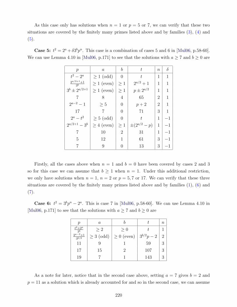
As this case only has solutions when n = 1 or p = 5 or 7, we can verify that these two
situations are covered by the finitely many primes listed above and by families (3), (4) and
(5).
Case 5: t2 = 2a + δ3bpn. This case is a combination of cases 5 and 6 in [Mul06, p.58-60].
We can use Lemma 4.10 in [Mul06, p.171] to see that the solutions with a ≥ 7 and b ≥ 0 are
p a b t n δ
t2 − 2a ≥ 1 (odd) 0 t 1 12a/2+1+1
3b≥ 1 (even) ≥ 1 2a/2 + 1 1 1
3b ± 2a/2+1 ≥ 1 (even) ≥ 1 p± 2a/2 1 1
7 8 4 65 2 1
2a−2 − 1 ≥ 5 0 p+ 2 2 1
17 7 0 71 3 1
2a − t2 ≥ 5 (odd) 0 t 1 −1
2a/2+1 − 3b ≥ 4 (even) ≥ 1 ±(2a/2 − p) 1 −1
7 10 2 31 1 −1
5 12 1 61 3 −1
7 9 0 13 3 −1
Firstly, all the cases above when n = 1 and b = 0 have been covered by cases 2 and 3
so for this case we can assume that b ≥ 1 when n = 1. Under this additional restriction,
we only have solutions when n = 1, n = 2 or p = 5, 7 or 17. We can verify that these three
situations are covered by the finitely many primes listed above and by families (1), (6) and
(7).
Case 6: t2 = 3bpn − 2a. This is case 7 in [Mul06, p.58-60]. We can use Lemma 4.10 in
[Mul06, p.171] to see that the solutions with a ≥ 7 and b ≥ 0 are
p a b t nt2+2a
3b≥ 2 ≥ 0 t 1
2a−2+13b/2
≥ 3 (odd) ≥ 0 (even) 3b/2p− 2 2
11 9 1 59 3
17 15 2 107 3
19 7 1 143 3
As a note for later, notice that in the second case above, setting a = 7 gives b = 2 and
p = 11 as a solution which is already accounted for and so in the second case, we can assume
220

that a − 1 ≥ 7. This case only has solutions when n = 1, n = 2 or p = 11, 17 or 19, and
thus we can verify that these three situations are covered by the finitely many primes listed
above and by family (9).
Case 7: 3t2 = ε2a + δp. This case is a combination of cases 10 to 12 in [Mul06, p.58-60].
We can use Lemma 4.11 in [Mul06, p.174-175] to see that the solutions with a ≥ 7 and b ≥ 0
are
p a t n δ ε
3t2 − 2a ≥ 0 t 1 1 1
11 8 23 3 1 1
2a − 3t2 ≥ 0 t 1 −1 1
5 7 1 3 −1 1
3t2 + 2a ≥ 0 t 1 1 −1
This case only has solutions when n = 1 or p = 5 or 11, and thus we can verify that
these three situations are covered by the finitely many primes listed above and by families
(10),(11) and (12).
Theorem 4.0.9. Let p be a prime distinct from 2 and 3. Then there exists an elliptic curve
with nontrivial rational two torsion of conductor 36p provided that p satisfies at least one of
the following where d > 0, n1 = 1 or Pmin(n1) ≥ 7, n2 ∈ 1, 2 and m1,m2 ≥ 0 are integers
with m1 odd and m2 even:
1. p = d2 + 4 · 3m2.
2. pn1 = d2 − 4 · 3m1.
3. pn1 = 4 · 3m1 − d2.
4. p = d2+3m1
4and p ≡ −1 (mod 4).
5. pn2 = 3d2+14
and p ≡ 1 (mod 4).
6. p = 3d2 − 4.
7. p ∈ 5, 13.
Theorem 4.0.10. Let p be a prime distinct from 2 and 3. Then up to the finitely many
primes in
p ∈ 5, 13
221

the following gives a complete list of the families of elliptic curves with nontrivial rational
two torsion of conductor 36p associated with the primes in the previous theorem:
(1) The prime p has the form p = d2 + 4 · 3m with m ≥ 0 even, d ∈ Z and corresponds to the
following elliptic curves
•a2 a4 ∆
C1 −3ψ(p− 4 · 3m) −3m+2 2432m+6p
C2 2 · 3ψ(p− 4 · 3m) 32p −283m+6p2
(2) The prime p has the form pn = d2− 4 · 3m with m ≥ 1 odd, n = 1 or Pmin(n) ≥ 7, d ∈ Zand corresponds to the following elliptic curves
•a2 a4 ∆
A1 −3ψ(4 · 3m + pn) 3m+2 2432m+6pn
A2 2 · 3ψ(4 · 3m + pn) 32pn 283m+6p2n
(3) The prime p has the form pn = 4 · 3m− d2 with m ≥ 1 odd, n = 1 or Pmin(n) ≥ 7, d ∈ Zand corresponds to the following elliptic curves
•a2 a4 ∆
B1 −3ψ(4 · 3m − pn) 3m+2 −2432m+6pn
B2 2 · 3ψ(4 · 3m − pn) −32pn 283m+6p2n
(4) The prime p has the form p = d2+3m
4with m ≥ 1 odd, p ≡ −1 (mod 4) and d ∈ Z and
corresponds to the following elliptic curves
•a2 a4 ∆
E1 −3ψ(4p− 3m) 32p −243m+6p2
E2 2 · 3ψ(4p− 3m) −3m+2 2832m+6p
(5) The prime p has the form pn = 3d2+14
with d an integer, n ∈ 1, 2, s ∈ 0, 1, p ≡1 (mod 4) and corresponds to the following elliptic curves
•a2 a4 ∆
I1 ε · 3s+1ψ(4pn−13
) 32s+1pn −2436s+3p2n
I2 −ε · 2 · 3s+1ψ(4pn−13
) −32s+1 2836s+3pn
where ε ∈ ±1 is the residue of 3s+1 modulo 4.
222

(6) The prime p has the form p = 3d2 − 4 with d an integer, s ∈ 0, 1 and corresponds to
the following elliptic curves
•a2 a4 ∆
J1 ε · 3s+1ψ(4+p3
) 32s+1 2436s+3p
J2 −ε · 2 · 3s+1ψ(4+p3
) 32s+1p 2836s+3p2
where ε ∈ ±1 is the residue of 3s+1 modulo 4.
Proof. To show this, we proceed in cases. We use the families in [Mul06, p.61-62] and simplify
them according to [Mul06, p.153-175].
Case 1: t2 = pn− 4 · 3b. This is case 4 in [Mul06, p.61-62]. Here b even is given. We can
use Lemma 4.9 in [Mul06, p.165] to see that the solutions with b ≥ 0 are
p b t n
t2 + 4 · 3b ≥ 0 t 1
5 0 11 3
13 5 35 3n√t2 + 4 · 3b ≥ 1 t Pmin(n) ≥ 7
According to [Luc02], we know that in the last case n < 5 and and thus this case gives
solutions only when n = 1 or p = 5 or 13. We can verify that these two situations are covered
by the finitely many primes listed above and by (1).
Case 2: t2 = 4 · 3b + δpn for δ ∈ ±1. This case is a combination of cases 1 and 2 in
[Mul06, p.61-62]. Here b odd is given. We can use Lemma 4.9 in [Mul06, p.165] to see that
the solutions with b ≥ 0 are
p b t n δ
t2 − 4 · 3b ≥ 0 t 1 1
13 1 47 3 1n√t2 − 4 · 3b ≥ 1 t Pmin(n) ≥ 7 1
4 · 3b − t2 ≥ 0 t 1 −1n√
4 · 3b − t2 ≥ 1 t Pmin(n) ≥ 7 −1
As this case only has solutions when n = 1, Pmin(n) ≥ 7 or p = 13, we can verify that
these two situations are covered by the finitely many primes listed above by (2) and by (3).
223

Case 3: t2 = 4pn−3b. This is case 3 in [Mul06, p.61-62]. Here pn ≡ −1 (mod 4) is given
and so the case n even is impossible. We can use Lemma 4.8 in [Mul06, p.156-157] to see
that the solutions with b ≥ 0 and n odd are
p b t n Extra Informationt2+3b
4≥ 1 (odd) t 1 p ≡ 1 (mod 3)
n
√t2+3b
4≥ 1 (odd) t Pmin(n) ≥ 7 p ≡ 1 (mod 3)
As shown in [AAA02], the second case cannot occur for n ≥ 7. As this case only has
solutions when n = 1, we can verify that this situation is covered by family (4).
Case 4: 3t2 = 4pn − 1. This is case 5 in [Mul06, p.61-62]. Here pn ≡ 1 (mod 4) is given.
By [Coh07a, p.353] Corollary 6.3.15, we have when n = 2 that
p = ε(σ2 + τ 2 + στ) 1 = δ(σ2 + τ 2 + 4στ)
with σ and τ of opposite parity and δ, ε ∈ ±1. We assume without loss of generality that
σ is the even term. In the second equation above, notice that if δ = −1, then modulo 4
considerations give us a contradiction. Hence δ = 1. Next assume towards a contradiction
that 2 ‖ σ. Then modulo 8, we have that 1 ≡ 4+1+0 ≡ 5 (mod 8) and that is a contradiction.
Hence 4 | σ. Further, in the equation above involving p, we have that σ2 + τ 2 + στ > 0 for
any integers σ and τ and so ε > 0. Combining this with 4 | σ shows us that
p = σ2 + τ 2 + στ ≡ 0 + 1 + 0 ≡ 1 (mod 4).
Thus p ≡ 1 (mod 4) when n = 2 and p ≡ 1 (mod 4) when n = 1 by necessity of this case.
We can use Lemma 4.11 in [Mul06, p.175] to see that the solutions are
p b t n3t2+1
4≥ 0 t 1√
3t2+14
≥ 1 t 2
As this case only has solutions when n = 1 or 2, we can verify that these two situations
are covered by family (5).
Case 5: 3t2 = pn + 4. This is case 6 in [Mul06, p.61-62]. We can use Lemma 4.11 in
[Mul06, p.174-175] to see that the only solutions are with p = 3t2 − 4. This situation is
covered by family (6).
224

Theorem 4.0.11. Let p be a prime distinct from 2 and 3. Then there exists an elliptic curve
with nontrivial rational two torsion of conductor 72p provided that p satisfies at least one of
the following where d > 0, `1 ∈ 2, 3, `2 ∈ 4, 5, `3 ∈ 2, 4, 5, n1 = 1 or Pmin(n1) ≥ 7,
n2 ∈ 1, 2 and m,m1 ≥ 0 are integers with m1 odd:
1. p = 2`13m + 1.
2. p = 2`13m − 1.
3. p = 3m + 2`1.
4. p = 3m − 2`1.
5. p = d2 + 2`33m.
6. pn1 = d2 − 2`23m.
7. pn1 = 2`23m − d2.
8. p = 3m1+14
.
9. p = 3m1+d2
4with p ≡ 1 (mod 4).
10. pn2 = 3d2+14
.
11. 1 pn1 = d2+323m
.
12. p = 3d2 + 2`3.
13. p = 3d2 − 2`2.
14. p ∈ 5, 7, 11, 13, 17, 23, 29, 31, 37, 47, 67, 73, 107, 109, 193, 1153.
Theorem 4.0.12. Let p be a prime distinct from 2 and 3. Then up to the finitely many
primes in
p ∈ 5, 7, 11, 13, 17, 23, 29, 31, 37, 47, 67, 73, 107, 109, 193, 1153
the following gives a complete list of the families of elliptic curves with nontrivial rational
two torsion of conductor 72p associated with the primes in the previous theorem:
(1) The prime p has the form p = 2`−2 · 3m + 1 with ` ∈ 4, 5, m ≥ 0 and corresponds to
the following elliptic curves
1In [BLM11, p.7], this case was erroneously claimed to be for odd m only. In fact cases such as m = 2and d = 11 do give valid elliptic curves.
225

•a2 a4 ∆
A1 −3ψ(2`3mp+ 1) 2`−23m+2p 22`32m+6p2
A2 2 · 3ψ(2`3mp+ 1) 32 2`+63m+6p
•a2 a4 ∆
G1 −3ψ(p2 − 2`3m) −2`−23m+2 22`32m+6p2
G2 2 · 3ψ(p2 − 2`3m) 32p2 −2`+63m+6p4
• In the additional case when ` − 2 = 2, we get solutions given by p = 2`3(2m)/2 + 1
and the curve is given by
a2 a4 ∆
B1 3ψ(4 · 3m + p) 32m+2 2434m+6p
B2 −2 · 3ψ(4 · 3m + p) 32p 2832m+6p2
(2) The prime p has the form p = 2`−2 · 3m − 1 with ` ∈ 4, 5, m ≥ 0 and corresponds to
the following elliptic curves
•a2 a4 ∆
A1 −3ψ(2`3mp+ 1) 2`−23m+2p 22`32m+6p2
A2 2 · 3ψ(2`3mp+ 1) 32 2`+63m+6p
•a2 a4 ∆
E1 −3ψ(2`3m + p2) 2`−23m+2 22`32m+6p2
E2 2 · 3ψ(2`3m + p2) 32p2 2`+63m+6p4
• In the additional case when `− 2 = 2, we get solutions given by p = 4 · 3(2m)/2 − 1
with m odd and the curve is given by
a2 a4 ∆
C1 3ψ(4 · 3m − pn) 32m+2 −2434m+6p
C2 −2 · 3ψ(4 · 3m − pn) −32p 2832m+6p2
(3) The prime p has the form p = 3m + 2`−2 with ` ∈ 4, 5, m ≥ 0 and corresponds to the
following elliptic curves
•a2 a4 ∆
G1 −3ψ(p2 − 2`3m) −2`−23m+2 22`32m+6p2
G2 2 · 3ψ(p2 − 2`3m) 32p2 −2`+63m+6p4
• In addition, replacing m above with 2m, then we get solutions with p = 3(2m)/2+2`−2
given by
226

a2 a4 ∆
K1 −3ψ(2`p+ 3m) 2`−232p 22`32m+6p2
K2 2 · 3ψ(2`p+ 3m) 32m+2 2`+634m+6p
• Rewriting `− 2 as ˆ/2 + 1, we get solutions with p = 3m + 2ˆ/2+1 given by
a2 a4 ∆
O1 −3ψ(2ˆ+ 3mp) 2
ˆ−232 22ˆ3m+6p
O2 2 · 3ψ(2ˆ+ 3mp) 3m+2p 2
ˆ+632m+6p2
(4) The prime p has the form p = 3m − 2`−2 with ` ∈ 4, 5, m ≥ 0 and corresponds to the
following elliptic curves
•a2 a4 ∆
E1 −3ψ(2`3m + p2) 2`−23m+2 22`32m+6p2
E2 2 · 3ψ(2`3m + p2) 32p2 2`+63m+6p4
• In addition, replacing m above with 2m, then we get solutions with p = 3(2m)/2+2`−2
given by
a2 a4 ∆
M1 −3ψ(3m − 2`pn) −2`−232p 22`32m+6p2
M2 2 · 3ψ(3m − 2`pn) 32m+2 −2`+634m+6p
• Rewriting `− 2 as ˆ/2 + 1, we get solutions with p = 3m + 2ˆ/2+1 given by
a2 a4 ∆
O1 −3ψ(2ˆ+ 3mp) 2
ˆ−232 22ˆ3m+6p
O2 2 · 3ψ(2ˆ+ 3mp) 3m+2p 2
ˆ+632m+6p2
(5) The prime p has the form p = d2 +2`3m with ` ∈ 2, 4, 5, m ≥ 0, d ∈ Z and corresponds
to the following elliptic curves
• In the case when ` = 2, we have
a2 a4 ∆
D1 3ψ(p− 4 · 3m) −3m+2 2432m+6p
D2 −2 · 3ψ(p− 4 · 3m) 32p −283m+6p2
• In the case when ` 6= 2, we have
227

a2 a4 ∆
G1 −3ψ(p− 2`3m) −2`−23m+2 22`32m+6p
G2 2 · 3ψ(p− 2`3m) 32p −2`+63m+6p2
(6) The prime p has the form pn = d2 − 2`3m with ` ∈ 4, 5, m ≥ 0, n = 1 or Pmin(n) ≥ 7,
d ∈ Z and corresponds to the following elliptic curves
•a2 a4 ∆
E1 −3ψ(2`3m + pn) 2`−23m+2 22`32m+6pn
E2 2 · 3ψ(2`3m + pn) 32pn 2`+63m+6p2n
(7) The prime p has the form pn = 2`3m − d2 with ` ∈ 4, 5, m ≥ 0, n = 1 or Pmin(n) ≥ 7,
d ∈ Z and corresponds to the following elliptic curves
•a2 a4 ∆
F1 −3ψ(2`3m − pn) 2`−23m+2 −22`32m+6pn
F2 2 · 3ψ(2`3m − pn) −32pn 2`+63m+6p2n
(8) The prime p has the form p = 3m+14
with m ≥ 1 odd and corresponds to the following
elliptic curves
•a2 a4 ∆
A1 −3ψ(243mp+ 1) 223m+2p 2832m+6p2
A2 2 · 3ψ(243mp+ 1) 32 2103m+6p
• If p ≡ 1 (mod 4) then also
a2 a4 ∆
I1 3ψ(4p2 − 3m) 32p2 −243m+6p4
I2 −2 · 3ψ(4p2 − 3m) −3m+2 2832m+6p2
• In addition, replacing m above with 2m, then we get solutions with p = 3(2m)/2+14
given by
a2 a4 ∆
K1 −3ψ(24p+ 32m) 2232p 2832m+6p2
K2 2 · 3ψ(24p+ 32m) 32m+2 21034m+6p
(9) The prime p has the form p = d2+3m
4with m ≥ 1 odd, p ≡ 1 (mod 4) and d ∈ Z and
corresponds to the following elliptic curves
228

•a2 a4 ∆
I1 3ψ(4p− 3m) 32p −243m+6p2
I2 −2 · 3ψ(4p− 3m) −3m+2 2832m+6p
(10) The prime p has the form pn = 3d2+14
with d an integer, n ∈ 1, 2, s ∈ 0, 1, and
corresponds to the following elliptic curves
•a2 a4 ∆
S1 −ε · 3s+1ψ(4pn−13
) 32s+1pn −2436s+3p2n
S2 ε · 2 · 3s+1ψ(4pn−13
) −32s+1 2836s+3pn
where ε ∈ ±1 is the residue of 3s+1 modulo 4.
(11) The prime p has the form pn = d2+323m
with m ≥ 0, n = 1 or Pmin(n) ≥ 7, d ∈ Z and
corresponds to the following elliptic curves
•a2 a4 ∆
Q1 −3ψ(3mpn − 25) −2332 2103m+6pn
Q2 2 · 3ψ(3mpn − 25) 3m+2pn −21132m+6p2n
(12) The prime p has the form p = 3d2−2` with ` ∈ 4, 5, s ∈ 0, 1, d ∈ Z and corresponds
to the following elliptic curves
•a2 a4 ∆
X1 ε · 3s+1ψ(2`+p3
) 2`−232s+1 22`36s+3p
X2 −ε · 2 · 3s+1ψ(2`+p3
) 32s+1p 2`+636s+3p2
where ε ∈ ±1 is the residue of 3s+1 modulo 4.
(13) The prime p has the form p = 3d2 + 2` with ` ∈ 2, 4, 5, s ∈ 0, 1, d ∈ Z and
corresponds to the following elliptic curves
• ` = 2 and
a2 a4 ∆
W1 −ε · 3s+1ψ(p−43
) −32s+1 2436s+3p
W2 ε · 2 · 3s+1ψ(p−43
) 32s+1p −2836s+3p2
where ε ∈ ±1 is the residue of 3s+1 modulo 4.
• ` ∈ 4, 5 and
229

a2 a4 ∆
Z1 ε · 3s+1ψ(p−2`
3) −2`−232s+1 22`36s+3p
Z2 −ε · 2 · 3s+1ψ(p−2`
3) 32s+1p −2`+636s+3p2
where ε ∈ ±1 is the residue of 3s+1 modulo 4.
Proof. To show this, we proceed in cases. We use the families in [Mul06, p.58-60] and simplify
them according to [Mul06, p.153-175]. In what follows, δ, ε ∈ ±1 not both negative.
Case 1: t2 = 2a3bpn + 1. This is case 1 in [Mul06, p.62-67]. We can use Lemma 4.7 in
[Mul06, p.153] to see that the solutions with a ∈ 4, 5 and b ≥ 0 are
p a b t n Extra Information3b+1
44 ≥ 0 odd 8p− 1 1 none
2a−2 · 3b ± 1 ≥ 3 ≥ 0 2p∓ 1 1 none
2a−2 ± 1 ≥ 5 0 2p∓ 1 1 none2a−2+1
3b≥ 5 ≥ 1 2a−1 + 1 1 3b|a− 2
5 4 0 9 1 none
5 5 1 49 2 none
Since we only care about cases when a = 4 or 5, in the fourth case above, since 3b|a− 2
and a = 5, the only case that this applies is a = 5 and b = 1. Here 2a−2+13b
= 3 is impossible
since p > 3. Further, cases two and three in the table above can be merged together. As this
case only has solutions when n = 1 or p = 5, we can verify that these situations are covered
by the finitely many primes listed above and families (1), (2) and (8).
Case 2: t2 = 4 · 3b + δpn. This is a combination of cases 2 and 4 in [Mul06, p.62-67].
Here b is given to be even. We can use Lemma 4.9 in [Mul06, p.165] to see that the solutions
with b ≥ 0 are
p b t n δ
t2 − 4 · 3b ≥ 0 t 1 1
13 0 47 3 1n√t2 − 4 · 3b ≥ 1 t Pmin(n) ≥ 7 1
4 · 3b − t2 ≥ 0 t 1 −1n√
4 · 3b − t2 ≥ 0 t Pmin(n) ≥ 7 −1
In the cases above when p 6= 13, notice that we have
pn = t2 − 4 · 3b = (t− 2 · 3b/2)(t+ 2 · 3b/2) or pn = 4 · 3b − t2 = (2 · 3b/2 − t)(2 · 3b/2 + t)
230

As the two factors are coprime, we have that t− 2 · 3b/2 = 1 or 2 · 3b/2− t = 1. Plugging this
into the original equation gives
pn = t2 − 4 · 3b = (2 · 3b/2 + 1)2 − 4 · 3b = 4 · 3b/2 + 1
which according to [Luc02] cannot occur when n ≥ 5 and so we can assume that n = 1 in
this case or
pn = 4 · 3b − t2 = 4 · 3b − (2 · 3b/2 − 1)2 = 4 · 3b/2 − 1.
Now, if b/2 is even, we can repeat the above procedure to get
pn = (2 · 3b/4 − 1)(2 · 3b/4 + 1)
and thus 2 · 3b/4 − 1 = 1 so b = 0 which gives p = 3, a contradiction. Hence in the second
case we must have that b/2 is odd. If b/2 < 5, then we see that
4 · 3b/2 + 1 ∈ 13, 37, 109, 325
(of which only 325 is not prime) or in the case with b/2 odd
4 · 3b/2 − 1 ∈ 11, 107
and all of these cases are in the list of finitely many primes. Next, suppose that b/2 ≥ 5. In
either case above, via [BVY04], we have that solutions of the form
pn + 4 · 3b/2(−1)n = (±1)3
correspond to newforms at level 6 which cannot occur. A summary of this result can be
found in [Coh07b, p.526-527]. Hence, this case only has solutions when n = 1 or p is in the
finitely many primes above. We can verify that these situations are covered by the finitely
many primes listed above and families (1) and (2).
Case 3: t2 = pn − 4 · 3b. This is case 13 in [Mul06, p.62-67]. Here b is given to be odd.
We can use Lemma 4.9 in [Mul06, p.165] to see that the solutions with b ≥ 0 are
p b t n
t2 + 4 · 3b ≥ 0 t 1
5 0 11 3
13 5 35 3n√t2 + 4 · 3b ≥ 0 t Pmin(n) ≥ 7
231

According to [Luc02], we know that in the final case n < 5 and so this case only has
solutions when n = 1 or p = 5 or 13. We can verify that these situations are covered by the
finitely many primes listed above and family (5).
Case 4: t2 = εpn + δ2a3b. This is a combination of cases 3,5, and 14 in [Mul06, p.62-67].
We can use Lemma 4.9 in [Mul06, p.165] to see that the solutions with a ∈ 4.5 and b ≥ 0
are
p a b t n δ ε
t2 − 2a · 3b ≥ 2 ≥ 0 t 1 1 1
2a−2 · 3b − 1 ≥ 3 ≥ 0 2a−1 + p 2 1 1
3b − 2a−2 ≥ 3 ≥ 0 2a−1 − p 2 1 1
2a−2 − 3b ≥ 5 ≥ 1 p+ 2 2 1 1n√t2 − 2a · 3b ≤ 5 ≥ 0 t Pmin(n) ≥ 7 1 1
t2 + 2a · 3b ≥ 1 ≥ 0 t 1 −1 1
2a−2 · 3b + 1 ≥ 3 ≥ 0 2a−1 + p 2 −1 1
3b + 2a−2 ≥ 3 ≥ 0 2a−1 − p 2 −1 1
73 4 7 595 3 −1 1
193 4 4 2681 3 −1 1
1153 5 5 39151 3 −1 1
5 5 1 23 4 −1 1n√t2 + 2a · 3b ≤ 5 ≥ 0 t Pmin(n) ≥ 7 −1 1
2a · 3b − t2 ≥ 1 ≥ 0 t 1 1 −1
73 5 11 2359 3 1 −1n√
2a · 3b − t2 ≤ 5 ≥ 0 t Pmin(n) ≥ 7 1 −1
As before, we can use [Luc02], we know that n < 5 when pn = t2 + 2a3b. Also, the case
where p = 2a−2 − 3b when a = 4 or 5 only gives the case p = 3, 5, or 7 and so this can be
simplified. Summarizing, this case only has solutions when n = 1, n = 2, Pmin(n) ≥ 7 or
p = 5, 7, 73, 193, or 1153, we can verify that these situations are covered by the finitely many
primes listed above and families (1), (2), (3), (4), (5), (6), and (7).
Case 5: t2 = 3b + δ2apn. This is a combination of cases 6 and 12 in [Mul06, p.62-67].
We can use Lemma 4.8 in [Mul06, p.156-157] to see that the solutions with a ∈ 4, 5 and
b ≥ 0 are
232

p a b t n δ3b/2+1
44 b/2 odd 3b/2 + 2 1 1
2a−2 ± 3b/2 ≥ 3 ≥ 0 even 2p∓ 3b/2 1 1
3b/2 − 2a−2 ≥ 3 ≥ 0 even ±(2p− 3b/2) 1 −1
In the second case above, we only need the positive case as the negative case gives solutions
p = 5 and p = 7, both of which are in the first family. As this case only has solutions when
n = 1 or p = 5 or 7 under the simplification above, we can verify that these situations are
covered by the finitely many primes listed above and families (3), (4) and (8).
Case 6: t2 = 4pn − 3b. This is case 7 in [Mul06, p.62-67]. We can use Lemma 4.8 in
[Mul06, p.156-157] to see that the solutions with b ≥ 0 are
p b t n Extra Informationt2+3b
4≥ 0 odd t 1 p ≡ 1 (mod 3)
3b+14
≥ 0 odd 2p− 1 2 none
n
√3b+1
4≥ 0 odd t Pmin(n) ≥ 7 p ≡ 1 (mod 3)
As shown in [AAA02], the third case cannot occur for n ≥ 7. All of the situations above
are covered in the family (8) and (9).
Case 7: t2 = 2a+ δ3bpn. This is a combination of cases 9 and 10 in [Mul06, p.62-67]. We
can use Lemma 4.10 in [Mul06, p.171-172] to see that the solutions with a ∈ 2, 4, 5 and
b ≥ 1 (possible to assume since we covered b = 0 in case 4) are
p a b t n δ
3b ± 4 2 ≥ 1 p∓ 2 1 1
3b ± 23 4 ≥ 1 p∓ 4 1 1
23 − 3b 4 ≥ 1 ±(4− p) 1 −1
The last case above only has positive solutions for b = 0 or b = 1 giving p = 7 or p = 5.
As this case only has solutions when n = 1 and a = 2, 4 or p = 5, or 7, we can verify that
these situations are covered by the finitely many primes listed above and families (3) and
(4).
Case 8: t2 = 3bpn − 2a. This is case 11 in [Mul06, p.62-67]. Now, we can assume that
b ≥ 1 since when b = 0, we can refer back to case 4. Notice that since b ≥ 1, we know that
233

a = 4 cannot happen by local considerations of the equation at 3. We can use Lemma 4.10
in [Mul06, p.156-157] to see that the solutions with a ∈ 4, 5 and b ≥ 1 are
p a b t nt2+2a
3b5 ≥ 1 t 1
2a−2+13b/2
5 ≥ 1 (even) 3b/2p− 2 2
67 5 3 8549 3
n
√t2+2a
3b5 ≥ 1 t Pmin(n) ≥ 7
As this case only has solutions when n = 1, Pmin(n) ≥ 7 or p = 17, we can verify that
these situations are covered by the finitely many primes listed above and family (11).
Case 9: 3t2 = 2a + δpn. This is a combination of cases 15 and 16 in [Mul06, p.62-67].
We can use Lemma 4.10 in [Mul06, p.174-175] to see that the solutions with a ∈ 4, 5 are
of the form p = δ(3t2 − 2a). When δ = −1 then since we are only considering cases with
a ∈ 4, 5, we only get the primes p = 13, 29. This situation is covered by family (13).
Case 10: 3t2 = pn − 2a. This is a combination of cases 18 and 19 in [Mul06, p.62-67].
We can use Lemma 4.10 in [Mul06, p.174-175] to see that the solutions with a ∈ 2, 4, 5 are
of the form p = 3t2 + 2a. This situation is covered by family (12).
Case 11: 3t2 = 4pn − 1. This is case 17 in [Mul06, p.62-67]. We can use Lemma 4.10
in [Mul06, p.174-175] to see that the solutions to this equation are of the form pn = 3t2 − 1
with n = 1 or 2. This situation is covered by family (10).
234

Chapter 5
Elliptic Curves With Rational Two
Torsion and Conductor 50p, 200p or
400p Organized by Primes
In this section, we continue our classification of elliptic curves with rational two torsion
and given conductor. Before beginning this section, I would like to remind the reader of the
notes of Chapter 4. These same notes apply here. In this section I suppress the formal proof
as well. These are done the same way as in the previous chapter except all of this work is
contained in this thesis.
Theorem 5.0.13. Let p be a prime distinct from 2 and 5. Then there exists an elliptic curve
with nontrivial rational two torsion of conductor 50p provided that p satisfies at least one of
the following where d > 0, `1 ≥ 5, `2 ≥ 7 and m ≥ 0 are integers:
1. p ∈ 3, 7, 11, 13, 17, 31, 37, 41
2. p = 2`15m + 1.
3. p = 2`15m − 1.
4. p = 2`1+15m
.
5. p = 2`1 − 5m.
6. p = 5m − 2`1.
7. p = 2`2 + 5m.
8. p = d2 − 2`25m.
9. p = 2`25m − d2.
235

10. p = d2 + 2`25m.
11. p = 5d2 − 2`2.
12. p = 2`2 − 5d2.
13. p = 5d2 + 2`2.
Theorem 5.0.14. Let p be a prime distinct from 2 and 5. Then up to the finitely many
primes in
p ∈ 3, 7, 11, 13, 17, 31, 37, 41
the following gives a complete list of the elliptic curves with nontrivial rational two torsion
of conductor 50p associated with the primes in the previous theorem:
(1) The prime p has the form p = 2`−2 · 5m + 1 with ` ≥ 7 and m ≥ 0 and corresponds to the
following elliptic curves
•a2 a4 ∆
A1 5ψ(2`5mp+ 1) 2`−25m+2p 22`52m+6p2
A2 −2 · 5ψ(2`5mp+ 1) 52 2`+65m+6p
•a2 a4 ∆
D1 5ψ(p2 − 2`5m) −2`−25m+2 22`52m+6p2
D2 −2 · 5ψ(p2 − 2`5m) 52p2 −2`+65m+6p4
(2) The prime p has the form p = 2`−2 · 5m− 1 with ` ≥ 7 and m ≥ 0 and corresponds to the
following elliptic curves
•a2 a4 ∆
A1 5ψ(2`5mp+ 1) 2`−25m+2p 22`52m+6p2
A2 −2 · 5ψ(2`5mp+ 1) 52 2`+65m+6p
•a2 a4 ∆
B1 5ψ(2`5m + p2) 2`−25m+2 22`52m+6p2
B2 −2 · 5ψ(2`5m + p2) 52p2 2`+65m+6p4
(3) The prime p has the form p = 2`−2+15m
with ` ≥ 7 and m ≥ 0 and corresponds to the
following elliptic curves
•a2 a4 ∆
A1 5ψ(2`5mp+ 1) 2`−25m+2p 22`52m+6p2
A2 −2 · 5ψ(2`5mp+ 1) 52 2`+65m+6p
236

• In addition, replacing m above with 2m, then we get solutions via p = 2`−2+15(2m)/2 given
by,
a2 a4 ∆
J1 5ψ(52mp2 − 2`) −2`−252 22`52m+6p2
J2 −2 · 5ψ(52mp2 − 2`) 52m+2p2 −2`+654m+6p4
(4) The prime p has the form p = 2`−2 − 5m with ` ≥ 7 and m ≥ 0 and corresponds to the
following elliptic curves
•a2 a4 ∆
B1 5ψ(2`5m + p2) 2`−25m+2 22`52m+6p2
B2 −2 · 5ψ(2`5m + p2) 52p2 2`+65m+6p4
• In addition, replacing m above with 2m, then we get solutions via p = 2`−2−5(2m)/2
given by,
a2 a4 ∆
E1 5ψ(2`p+ 52m) 2`−252p 22`52m+6p2
E2 −2 · 5ψ(2`p+ 52m) 52m+2 2`+654m+6p
• In the additional case that `−2 can be written as ˆ/2+1 with ˆeven, we get solutions
with p = 2`/2+1 − 5m given by
a2 a4 ∆
I1 5ψ(2ˆ− 5mp) 2
ˆ−252 −22ˆ5m+6p
I2 −2 · 5ψ(2ˆ− 5mp) −5m+2p 2
ˆ+652m+6p2
for this new `
(5) The prime p has the form p = 5m − 2`−2 with ` ≥ 7 and m ≥ 0 and corresponds to the
following elliptic curves
•a2 a4 ∆
B1 5ψ(2`5m + p2) 2`−25m+2 22`52m+6p2
B2 −2 · 5ψ(2`5m + p2) 52p2 2`+65m+6p4
• In addition, replacing m above with 2m, then we get solutions with p = 5(2m)/2−2`−2
given by
a2 a4 ∆
G1 5ψ(52m − 2`p) −2`−252p 22`52m+6p2
G2 −2 · 5ψ(52m − 2`p) 52m+2 −2`+654m+6p
237

• In the additional case that `−2 can be written as ˆ/2+1 with ˆeven, we get solutions
with p = 5m − 2ˆ/2+1 given by
a2 a4 ∆
H1 5ψ(2ˆ+ 5mp) 2
ˆ−252 22ˆ5m+6p
H2 −2 · 5ψ(2ˆ+ 5mp) 5m+2p 2
ˆ+652m+6p2
(6) The prime p has the form p = 2`−2 + 5m with ` ≥ 7 and m ≥ 0 and corresponds to the
following elliptic curves
•a2 a4 ∆
D1 5ψ(p2 − 2`5m) −2`−25m+2 22`52m+6p2
D2 −2 · 5ψ(p2 − 2`5m) 52p2 −2`+65m+6p4
• In addition, replacing m above with 2m, then we get solutions with p = 2`−2+5(2m)/2
given by
a2 a4 ∆
E1 5ψ(2`p+ 52m) 2`−252p 22`52m+6p2
E2 −2 · 5ψ(2`p+ 52m) 52m+2 2`+654m+6p
• In the additional case that `−2 can be written as ˆ/2+1 with ˆeven, we get solutions
with p = 2ˆ/2+1 + 5m given by
a2 a4 ∆
H1 5ψ(2ˆ+ 5mp) 2
ˆ−252 22ˆ5m+6p
H2 −2 · 5ψ(2ˆ+ 5mp) 5m+2p 2
ˆ+652m+6p2
(7) The prime p has the form p = d2 − 2`5m with ` ≥ 7, m ≥ 0 and d ∈ Z and corresponds
to the following elliptic curves
•a2 a4 ∆
B1 5ψ(2`5m + p) 2`−25m+2 22`52m+6p
B2 −2 · 5ψ(2`5m + p) 52p 2`+65m+6p2
(8) The prime p has the form p = 2`5m − d2 with ` ≥ 7, m ≥ 0 and d ∈ Z and corresponds
to the following elliptic curves
•a2 a4 ∆
C1 5ψ(2`5m − p) 2`−25m+2 −22`52m+6p
C2 −2 · 5ψ(2`5m − p) −52p 2`+65m+6p2
(9) The prime p has the form p = d2 + 2`5m with ` ≥ 7, m ≥ 0 and d ∈ Z and corresponds
to the following elliptic curves
238

•a2 a4 ∆
D1 5ψ(p− 2`5m) −2`−25m+2 22`52m+6p
D2 −2 · 5ψ(p− 2`5m) 52p −2`+65m+6p2
(10) The prime p has the form p = 5d2 − 2` with ` ≥ 7, m ≥ 0, d ∈ Z and s ∈ 0, 1 and
corresponds to the following elliptic curves
•a2 a4 ∆
M1 5s+1ψ(2`+p5
) 2`−252s+1 22`56s+3p
M2 −2 · 5s+1ψ(2`+p5
) 52s+1p 2`+656s+3p2
(11) The prime p has the form p = 2` − 5d2 with ` ≥ 7, m ≥ 0, d ∈ Z and s ∈ 0, 1 and
corresponds to the following elliptic curves
•a2 a4 ∆
N1 5s+1ψ(2`−p5
) 2`−252s+1 −22`56s+3p
N2 −2 · 5s+1ψ(2`−p5
) −52s+1p 2`+656s+3p2
(12) The prime p has the form p = 5d2 + 2` with ` ≥ 7, m ≥ 0, d ∈ Z and s ∈ 0, 1 and
corresponds to the following elliptic curves
•a2 a4 ∆
O1 5s+1ψ(p−2`
5) −2`−252s+1 22`56s+3p
O2 −2 · 5s+1ψ(p−2`
5) 52s+1p −2`+656s+3p2
Theorem 5.0.15. Let p be a prime distinct from 2 and 5. Then there exists an elliptic curve
with nontrivial rational two torsion of conductor 200p provided that p satisfies at least one of
the following where d > 0, `1 ∈ 2, 4, 5, `2 ∈ 4, 5, `3 ∈ 3, 4, 5 and m ≥ 0 are integers:
1. p ∈ 3, 7, 11, 13, 17, 23, 31, 37, 41.
2. p = 2`2−2 · 5m + 1 with m ≥ 1.
3. p = 2`2−2 · 5m − 1 with m ≥ 1.
4. pn = 5m−14
with m ≥ 1 odd and n = 1 or Pmin(n) ≥ 7.
5. pn =(
5m−14
)2with n = 2 or 2 ‖ n and Pmin(n/2) ≥ 7.
6. pn = d2−5m
4with m odd and either n = 1 or Pmin(n) ≥ 7.
7. pn = 5m−d24
with m odd and either n = 1 or Pmin(n) ≥ 7 or n even.
8. pn = 5m−d22`2
with m even and Pmin(n) ≥ 7.
239

9. pn = 2`2−2 + 5m with m ≥ 1 and either n = 1 or Pmin(n) ≥ 7.
10. pn = 5m − 2`2−2 with m ≥ 1 and either n = 1 or both `2 = 4 and Pmin(n) ≥ 7.
11. pn = (5m − 4)2 with m ≥ 1 and either n = 2 or 2 ‖ n and Pmin(n/2) ≥ 7.
12. pn = d2 − 2`15m with n = 1 or Pmin(n) ≥ 7.
13. pn = 2`15m − d2 with n = 1 or Pmin(n) ≥ 7.
14. p = d2 + 2`15m.
15. pn = d2+45m
with m ≥ 1 odd and either n = 2 or 2 ‖ n and Pmin(n/2) ≥ 7.
16. pn = d2+2`15m
with m ≥ 1 and either n = 1 or Pmin(n) ≥ 7.
17. pn = 5d2−14
with pn ≡ 1 (mod 4) and n = 1, n = 2, Pmin(n) ≥ 7 or both 2 ‖ n and
Pmin(n/2) ≥ 7.
18. pn = 5d2 − 2`1 with either n = 1 or Pmin(n) ≥ 7.
19. pn = 5d2 − 4 with either n = 2 or 2 ‖ n and Pmin(n/2) ≥ 7.
20. pn = 5d2 + 2`2 with either n = 1 or Pmin(n) ≥ 7.
21. pn = 5d2 + 4 with either n = 2 or 2 ‖ n and Pmin(n/2) ≥ 7.
Theorem 5.0.16. Let p be a prime distinct from 2 and 5. Then up to the finitely many
primes in
p ∈ 3, 7, 11, 13, 17, 23, 31, 37, 41
the following gives a complete list of the elliptic curves with nontrivial rational two torsion
of conductor 200p associated with the primes in the previous theorem:
(1) The prime p has the form p = 2`−2 · 5m + 1 with ` ∈ 4, 5 and m > 0 and corresponds
to the following elliptic curves
•a2 a4 ∆
A1 5ψ(2`5mp+ 1) 2`−25m+2p 22`52m+6p2
A2 −2 · 5ψ(2`5mp+ 1) 52 2`+65m+6p
•a2 a4 ∆
G1 5ψ(p2 − 2`5m) −2`−25m+2 22`52m+6p2
G2 −2 · 5ψ(p2 − 2`5m) 52p2 −2`+65m+6p4
240

(2) The prime p has the form p = 2`−2 · 5m − 1 with ` ∈ 4, 5 and m > 0 and corresponds
to the following elliptic curves
•a2 a4 ∆
A1 5ψ(2`5mp+ 1) 2`−25m+2p 22`52m+6p2
A2 −2 · 5ψ(2`5mp+ 1) 52 2`+65m+6p
•a2 a4 ∆
E1 5ψ(2`5m + pn) 2`−25m+2 22`52m+6p2
E2 −2 · 5ψ(2`5m + pn) 52p2 2`+65m+6p4
(3) The prime p has the form pn = 5m−14
with and m ≥ 1 odd and corresponds to the following
elliptic curves
• Either n = 1 or Pmin(n) ≥ 7 and the curve is given by
a2 a4 ∆
A1 5ψ(2`5mpn + 1) 225m+2pn 2852m+6p2n
A2 −2 · 5ψ(2`5mpn + 1) 52 2105m+6pn
• n = 1 and the curve is given by
a2 a4 ∆
H1 −5ψ(4p2 + 5m) 52p2 245m+6p4
H2 2 · 5ψ(4p2 + 5m) 5m+2 2852m+6p2
• We have n = 1 and in addition, replacing m above with 2m, then we get solutions
via p = 5(2m)/2−14
given by,
a2 a4 ∆
M1 5ψ(52m − 24pn) −2252p 2852m+6p2
M2 −2 · 5ψ(52m − 24pn) 52m+2 −21054m+6p
(4) The prime p has the form pn =(
5m−14
)2with and m ≥ 1 odd, n = 2 or 2 ‖ n and
Pmin(n/2) ≥ 7 and corresponds to the following elliptic curves
•a2 a4 ∆
H1 −5ψ(4pn + 5m) 52pn 245m+6p2n
H2 2 · 5ψ(4pn + 5m) 5m+2 2852m+6pn
(5) The prime p has the form pn = d2−5m
4with m ≥ 1 odd and d ∈ Z and corresponds to the
following elliptic curves
241

• Either n = 1 or Pmin(n) ≥ 7 and the curve is given by
a2 a4 ∆
H1 −5ψ(4pn + 5m) 52pn 245m+6p2n
H2 2 · 5ψ(4pn + 5m) 5m+2 2852m+6pn
(6) The prime p has the form pn = 5m−d24
with m ≥ 1 odd and d ∈ Z and corresponds to the
following elliptic curves
• Either n = 1, Pmin(n) ≥ 7 or n is even, m is odd and the curve is given by
a2 a4 ∆
J1 −5ψ(5m − 4pn) −52pn 245m+6p2n
J2 2 · 5ψ(5m − 4pn) 5m+2 −2852m+6pn
(7) The prime p has the form pn = 5m−d22`
with ` ∈ 4, 5, m even, Pmin(n) ≥ 7 and corre-
sponds to the following elliptic curve
•a2 a4 ∆
M1 5ψ(5m − 2`pn) −2`−252pn 22`5m+6p2n
M2 −2 · 5ψ(5m − 2`pn) 5m+2 −2`+652m+6pn
(8) The prime p has the form pn = 2`−2+5m with and m ≥ 1 and corresponds to the following
elliptic curves
• n = 1, ` ∈ 4, 5 and
a2 a4 ∆
G1 5ψ(p2 − 2`5m) −2`−25m+2 22`52m+6p2
G2 −ε · 2 · 5ψ(p2 − 2`5m) 52p2 −2`+65m+6p4
• n = 1 or Pmin(n) ≥ 7, ` ∈ 4, 5 with pn = 2`−2 + 5(2m)/2 and
a2 a4 ∆
K1 5ψ(2`pn + 5m) 2`−252pn 22`52m+6p2n
K2 −ε · 2 · 5ψ(2`pn + 5m) 52m+2 2`+654m+6pn
• ` = 4 so `− 2 = 2, n = 1 or Pmin(n) ≥ 7 and
a2 a4 ∆
N1 −5ψ(4 + 5mpn) 52 245m+6pn
N2 2 · 5ψ(4 + 5mpn) 5m+2pn 2852m+6p2n
• n = 1, ` = 5 so `− 2 = 3 = 4/2 + 1 and
242

a2 a4 ∆
O1 5ψ(16 + 5mp) 2252 285m+6p
O2 −2 · 5ψ(16 + 5mp) 5m+2p 21052m+6p2
(9) The prime p has the form pn = 5m−2`−2 with and m ≥ 1 and corresponds to the following
elliptic curves
• n = 1 and ` ∈ 4, 5 and the elliptic curve is given by
a2 a4 ∆
M1 5ψ(5m − 2`p) −2`−252p 22`5m+6p2
M2 −2 · 5ψ(5m − 2`p) 5m+2 −2`+652m+6p
• Either n = 1 or Pmin(n) ≥ 7 and ` = 4 so `− 2 = 2 = 2/2 + 1giving
a2 a4 ∆
N1 −5ψ(4 + 5mpn) 52 245m+6pn
N2 2 · 5ψ(4 + 5mpn) 5m+2pn 2852m+6p2n
• n = 1 with ` ∈ 4, 5 and the elliptic curve is given by
a2 a4 ∆
E1 5ψ(2`5m + p) 2`−25m+2 22`52m+6p
E2 −2 · 5ψ(2`5m + p) 52p 2`+65m+6p2
• n = 1, ` = 5 and so `− 2 = 3 = 4/2 + 1 and
a2 a4 ∆
O1 5ψ(16 + 5mp) 2252 285m+6p
O2 −2 · 5ψ(16 + 5mp) 5m+2p 21052m+6p2
(10) The prime p has the form pn = (5m − 4)2 with m ≥ 1 odd and either n = 2 or 2 ‖ n and
Pmin(n/2) ≥ 7 and corresponds to the following elliptic curve
a2 a4 ∆
E1 5ψ(245m + pn) 225m+2 2852m+6pn
E2 −2 · 5ψ(245m + pn) 52pn 2105m+6p2n
(11) The prime p has the form pn = d2 − 2` · 5m with m ≥ 0, d ∈ Z, ` ∈ 2, 4, 5 and either
n = 1 or Pmin(n) ≥ 7 and corresponds to the following elliptic curves
• ` = 2 and
243
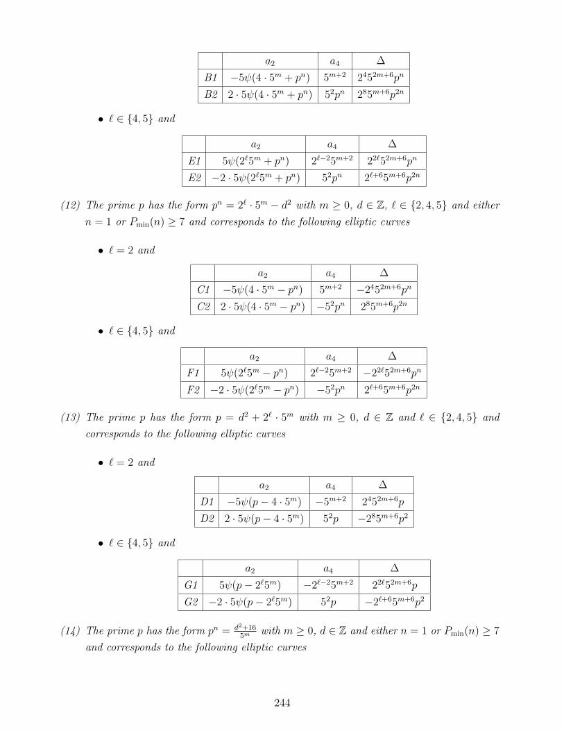
a2 a4 ∆
B1 −5ψ(4 · 5m + pn) 5m+2 2452m+6pn
B2 2 · 5ψ(4 · 5m + pn) 52pn 285m+6p2n
• ` ∈ 4, 5 and
a2 a4 ∆
E1 5ψ(2`5m + pn) 2`−25m+2 22`52m+6pn
E2 −2 · 5ψ(2`5m + pn) 52pn 2`+65m+6p2n
(12) The prime p has the form pn = 2` · 5m − d2 with m ≥ 0, d ∈ Z, ` ∈ 2, 4, 5 and either
n = 1 or Pmin(n) ≥ 7 and corresponds to the following elliptic curves
• ` = 2 and
a2 a4 ∆
C1 −5ψ(4 · 5m − pn) 5m+2 −2452m+6pn
C2 2 · 5ψ(4 · 5m − pn) −52pn 285m+6p2n
• ` ∈ 4, 5 and
a2 a4 ∆
F1 5ψ(2`5m − pn) 2`−25m+2 −22`52m+6pn
F2 −2 · 5ψ(2`5m − pn) −52pn 2`+65m+6p2n
(13) The prime p has the form p = d2 + 2` · 5m with m ≥ 0, d ∈ Z and ` ∈ 2, 4, 5 and
corresponds to the following elliptic curves
• ` = 2 and
a2 a4 ∆
D1 −5ψ(p− 4 · 5m) −5m+2 2452m+6p
D2 2 · 5ψ(p− 4 · 5m) 52p −285m+6p2
• ` ∈ 4, 5 and
a2 a4 ∆
G1 5ψ(p− 2`5m) −2`−25m+2 22`52m+6p
G2 −2 · 5ψ(p− 2`5m) 52p −2`+65m+6p2
(14) The prime p has the form pn = d2+165m
with m ≥ 0, d ∈ Z and either n = 1 or Pmin(n) ≥ 7
and corresponds to the following elliptic curves
244

•a2 a4 ∆
Q1 5ψ(5mpn − 16) −2252 285m+6pn
Q2 −2 · 5ψ(5mpn − 16) 5m+2pn −21052m+6p2n
(15) The prime p has the form pn = 5d2−14
with pn ≡ 1 (mod 4), s ∈ 0, 1, one of n = 1,
n = 2, Pmin(n) ≥ 7 or 2 ‖ n and Pmin(n/2) ≥ 7 and corresponds to the following elliptic
curves
•a2 a4 ∆
R1 −5s+1ψ(4pn+15
) 52s+1pn 2456s+3p2n
R2 2 · 5s+1ψ(4pn+15
) 52s+1 2856s+3pn
(16) The prime p has the form pn = 5d2 − 2` with ` ∈ 2, 4, 5, s ∈ 0, 1 and either n = 1
or Pmin(n) ≥ 7 and corresponds to the following elliptic curves
• ` = 2 and
a2 a4 ∆
V1 −5s+1ψ(4+pn
5) 52s+1 2456s+3pn
V2 2 · 5s+1ψ(4+pn
5) 52s+1pn 2856s+3p2n
• ` ∈ 4, 5 and
a2 a4 ∆
X1 5s+1ψ(2`+pn
5) 2`−252s+1 22`56s+3pn
X2 −2 · 5s+1ψ(2`+pn
5) 52s+1pn 2`+656s+3p2n
(17) The prime p has the form pn = 5d2 + 2` with ` ∈ 4, 5, s ∈ 0, 1 and either n = 1 or
Pmin(n) ≥ 7 and corresponds to the following elliptic curves
•a2 a4 ∆
Z1 5s+1ψ(pn−2`
5) −2`−252s+1 22`56s+3pn
Z2 −2 · 5s+1ψ(pn−2`
5) 52s+1pn −2`+656s+3p2n
Theorem 5.0.17. Let p be a prime distinct from 2 and 5. Then there exists an elliptic curve
with nontrivial rational two torsion of conductor 400p provided that p satisfies at least one
of the following where d > 0, `1 ≥ 2, `2 ≥ 4, `3 = λ with λ = 2 or λ ≥ 4 and m ≥ 0 are
integers:
1. p ∈ 3, 7, 11, 13, 17, 23, 31, 37, 41.
2. p = 2`15m + 1.
245

3. p = 2`15m − 1.
4. p = 2`1+15m
.
5. pn = 5m−14
with m odd and n = 1 or Pmin(n) ≥ 7.
6. pn =(
5m−14
)2with m ≥ 1 and n = 2 or 2 ‖ n and Pmin(n/2) ≥ 7.
7. pn = d2−5m
4with m odd and either n = 1 or Pmin(n) ≥ 7.
8. pn = 5m−d24
with m odd and either n = 1, Pmin(n) ≥ 7 or n even.
9. pn = 5m−d22`3
with `3 ∈ 4, 5, m even and either n = 1 or Pmin(n) ≥ 7.
10. pn = 2`1 + 5m with n = 1 or Pmin(n) ≥ 7.
11. pn = 2`1 − 5m with n = 1 or Pmin(n) ≥ 7.
12. p = 5m − 2`2 with n = 1 or both Pmin(n) ≥ 7 and `1 = 2.
13. pn = (5m − 4)2 with n = 2 or 2 ‖ n and Pmin(n/2) ≥ 7.
14. pn = d2 − 2`35m with either n = 1 or both Pmin(n) ≥ 7 and `3 ∈ 2, 4, 5.
15. pn = 2`35m − d2 with either n = 1 or both Pmin(n) ≥ 7 and `3 ∈ 2, 4, 5.
16. p = d2 + 2`35m.
17. pn = d2+2`35m
with m ≥ 1, n = 1 or Pmin(n) ≥ 7.
18. pn = d2+45m
with m ≥ 1 odd and either n = 2 or 2 ‖ n and Pmin(n/2) ≥ 7.
19. pn = 5d2−14
with pn ≡ 1 (mod 4) and one of n = 1, n = 2, Pmin(n) ≥ 7 or 2 ‖ n and
Pmin(n/2) ≥ 7.
20. pn = 5d2 − 2`3 with n = 1 or both Pmin(n) ≥ 7 and `3 ∈ 4, 5.
21. pn = 5d2 − 4 with n = 2 or 2 ‖ n and Pmin(n/2) ≥ 7.
22. p = 2`3 − 5d2.
23. pn = 5d2 + 2`3 with n = 1 or both Pmin(n) ≥ 7 and `3 ∈ 4, 5.
24. pn = 5d2 + 4 with n = 2 or 2 ‖ n and Pmin(n/2) ≥ 7.
246

Theorem 5.0.18. Let p be a prime distinct from 2 and 5. Then up to the finitely many
primes in
p ∈ 3, 7, 11, 13, 17, 23, 31, 37, 41
the following gives a complete list of the elliptic curves with nontrivial rational two torsion
of conductor 400p associated with the primes in the previous theorem:
(1) The prime p has the form p = 2`−2 · 5m + 1 with ` ≥ 4 and m ≥ 0 and corresponds to the
following elliptic curves
•a2 a4 ∆
A1 −5ψ(2`5mp+ 1) 2`−25m+2p 22`52m+6p2
A2 2 · 5ψ(2`5mp+ 1) 52 2`+65m+6p
•a2 a4 ∆
G1 −5ψ(p2 − 2`5m) −2`−25m+2 22`52m+6p2
G2 2 · 5ψ(p2 − 2`5m) 52p2 −2`+65m+6p4
(2) The prime p has the form p = 2`−2 · 5m− 1 with ` ≥ 4 and m ≥ 0 and corresponds to the
following elliptic curves
•a2 a4 ∆
A1 −5ψ(2`5mp+ 1) 2`−25m+2p 22`52m+6p2
A2 2 · 5ψ(2`5mp+ 1) 52 2`+65m+6p
•a2 a4 ∆
E1 −5ψ(2`5m + p2) 2`−25m+2 22`52m+6p2
E2 2 · 5ψ(2`5m + p2) 52p2 2`+65m+6p4
(3) The prime p has the form p = 2L+15m
with L,m ≥ 0 and corresponds to the following
elliptic curves
• If L = `− 2 for ` ≥ 4 even, then
a2 a4 ∆
A1 −5ψ(2`5mp+ 1) 2`−25m+2p 22`52m+6p2
A2 2 · 5ψ(2`5mp+ 1) 52 2`+65m+6p
• If L = `/2 for ` ≥ 4 even and p = 2`/2+15(2m)/2 giving
a2 a4 ∆
R1 −5ψ(52mpn − 2`) −2`−252 22`52m+6p2
R2 2 · 5ψ(52mpn − 2`) 52m+2p2 −2`+654m+6p4
247

(4) The prime p has the form pn = 5m−14
with m > 0 odd and corresponds to the following
elliptic curves
• Either n = 1 or Pmin(n) ≥ 7 and
a2 a4 ∆
A1 −5ψ(2`5mpn + 1) 225m+2pn 2852m+6p2n
A2 2 · 5ψ(2`5mpn + 1) 52 2105m+6pn
• n = 1, p ≡ 1 (mod 4) and
a2 a4 ∆
J1 5ψ(5m − 4p) −52p 245m+6p2
J2 −2 · 5ψ(5m − 4p) 5m+2 −2852m+6p
• n = 1 and we have a solution with p = 5(2m)/2−14
given by
a2 a4 ∆
M1 −5ψ(52m − 16p) −2252p 2852m+6p2
M2 2 · 5ψ(52m − 16p) 52m+2 −21054m+6p
(5) The prime p has the form pn =(
5m−14
)2with m ≥ 1 odd and either n = 2 or 2 ‖ n and
Pmin(n/2) ≥ 7 and corresponds to the following curve
•a2 a4 ∆
J1 5ψ(5m − 4pn) −52pn 245m+6p2n
J2 −2 · 5ψ(5m − 4pn) 5m+2 −2852m+6pn
(6) The prime p has the form pn = d2−5m
4with m > 0 odd, n = 1 or Pmin(n) ≥ 7 and
corresponds to the following elliptic curves
•a2 a4 ∆
H1 5ψ(4pn + 5m) 52pn 245m+6p2n
H2 −2 · 5ψ(4pn + 5m) 5m+2 2852m+6pn
(7) The prime p has the form pn = 5m−d24
with m ≥ 0 and either n = 1 or both m is odd and
Pmin(n) ≥ 7 and corresponds to the following elliptic curve
•a2 a4 ∆
J1 5ψ(5m − 4pn) −52pn 245m+6p2n
J2 −2 · 5ψ(5m − 4pn) 5m+2 −2852m+6pn
248

(8) The prime p has the form pn = 5m−d22`
with m ≥ 0, ` ∈ 4, 5 and Pmin(n) ≥ 7 and
corresponds to the following elliptic curve
•a2 a4 ∆
M1 −5ψ(5m − 2`pn) −2`−252pn 22`52m+6p2n
M2 2 · 5ψ(5m − 2`pn) 52m+2 −2`+654m+6pn
(9) The prime p has the form pn = 2L + 5m with L > 0, m ≥ 0 and corresponds to the
following elliptic curves
• If L = `− 2, ` ≥ 4 and in this case pn = 2`−2 + 5(2m)/2 with n = 1 or Pmin(n) ≥ 7
and ` ∈ 4, 5, then we have
a2 a4 ∆
K1 −5ψ(2`pn + 52m) 2`−252pn 22`52m+6p2n
K2 2 · 5ψ(2`pn + 52m) 52m+2 2`+654m+6pn
• If L = `− 2, ` ≥ 4, and n = 1, then
a2 a4 ∆
G1 −5ψ(p2 − 2`5m) −2`−25m+2 22`52m+6p2
G2 2 · 5ψ(p2 − 2`5m) 52p2 −2`+65m+6p4
• If L = `/2 + 1 for ` ≥ 4 even and n = 1, then
a2 a4 ∆
P1 −5ψ(2` + 5mp) 2`−252 22`5m+6p
P2 2 · 5ψ(2` + 5mp) 5m+2p 2`+652m+6p2
• If L = 2 and n = 1 or Pmin(n) ≥ 7, then we have
a2 a4 ∆
N1 5ψ(4 + 5mpn) 52 245m+6pn
N2 −2 · 5ψ(4 + 5mpn) 5m+2pn 2852m+6p2n
(10) The prime p has the form pn = 2L − 5m with L > 0, m ≥ 0 and corresponds to the
following elliptic curves
• If n = 1 and L = `− 2 ≥ 2 hold we have
a2 a4 ∆
E1 −5ψ(2`5m + p2) 2`−25m+2 22`52m+6p2
E2 2 · 5ψ(2`5m + p2) 52p2 2`+65m+6p4
249

• If L = `− 2, ` ≥ 4 and in this case pn = 2`−2 + 5(2m)/2 with n = 1 or Pmin(n) ≥ 7
and ` ∈ 4, 5, then we have
a2 a4 ∆
K1 −5ψ(2`pn + 52m) 2`−252pn 22`52m+6p2n
K2 2 · 5ψ(2`pn + 52m) 52m+2 2`+654m+6pn
• If n = 1 and L = `− 2 with ` ≥ 4, then we have
a2 a4 ∆
G1 −5ψ(p2 − 2`5m) −2`−25m+2 22`52m+6p2
G2 2 · 5ψ(p2 − 2`5m) 52p2 −2`+65m+6p4
• If n = 1 and L = `/2 + 1 for ` ≥ 4 even we have
a2 a4 ∆
Q1 −5ψ(2` − 5mp) 2`−252 −22`5m+6p
Q2 2 · 5ψ(2` − 5mp) −5m+2p 2`+652m+6p2
(11) The prime p has the form pn = 5m − 2L with L > 0, m ≥ 0 and corresponds to the
following elliptic curves
• If L = `− 2, ` ≥ 4 and in this case p = 5(2m)/2 − 2`−2, then we have
a2 a4 ∆
M1 −5ψ(52m − 2`p) −2`−252p 22`52m+6p2
M2 2 · 5ψ(52m − 2`p) 52m+2 −2`+654m+6p
• If n = 1 and L = `− 2 ≥ 2 hold we have
a2 a4 ∆
E1 −5ψ(2`5m + p2) 2`−25m+2 22`52m+6p2
E2 2 · 5ψ(2`5m + p2) 52p2 2`+65m+6p4
• If L = `/2 + 1 for ` ≥ 4 even with n = 1, we have
a2 a4 ∆
P1 −5ψ(2` + 5mp) 2`−252 22`5m+6p
P2 2 · 5ψ(2` + 5mp) 5m+2p 2`+652m+6p2
• If L = 2 and n = 1 or Pmin(n) ≥ 7, then we have
a2 a4 ∆
N1 5ψ(4 + 5mpn) 52 245m+6pn
N2 −2 · 5ψ(4 + 5mpn) 5m+2pn 2852m+6p2n
250

(12) The prime p has the form pn = (5m − 4)2 with m ≥ 0 odd, n = 2 or 2 ‖ n and
Pmin(n/2) ≥ 7 and corresponds to the following elliptic curve
a2 a4 ∆
E1 −5ψ(16 · 5m + pn) 225m+2 2852m+6pn
E2 2 · 5ψ(16 · 5m + pn) 52pn 2105m+6p2n
(13) The prime p has the form pn = d2−2`5m with ` = 2 or ` ≥ 4 and m ≥ 0 and corresponds
to the following elliptic curves
• Either n = 1 and ` ≥ 4 or Pmin(n) ≥ 7 and ` ∈ 4, 5 and
a2 a4 ∆
E1 −5ψ(2`5m + pn) 2`−25m+2 22`52m+6pn
E2 2 · 5ψ(2`5m + pn) 52pn 2`+65m+6p2n
• ` = 2 and either n = 1 or Pmin(n) ≥ 7 and the elliptic curve is given by
a2 a4 ∆
B1 5ψ(4 · 5m + pn) 5m+2 2452m+6pn
B2 −2 · 5ψ(4 · 5m + pn) 52pn 285m+6p2n
(14) The prime p has the form pn = 2`5m−d2 with ` = 2 or ` ≥ 4 and m ≥ 0 and corresponds
to the following elliptic curves
• Either n = 1 or Pmin(n) ≥ 7, ` = 2 and p ≡ 3 (mod 8)
a2 a4 ∆
C1 5ψ(4 · 5m − pn) 5m+2 −2452m+6pn
C2 −2 · 5ψ(4 · 5m − pn) −52pn 285m+6p2n
• Either n = 1 with ` ≥ 4 or Pmin(n) ≥ 7 with ` ∈ 4, 5, p ≡ 7 (mod 8) and the
elliptic curve is given by
a2 a4 ∆
F1 −5ψ(2`5m − pn) 2`−25m+2 −22`52m+6pn
F2 2 · 5ψ(2`5m − pn) −52pn 2`+65m+6p2n
(15) The prime p has the form p = d2 + 2`5m with ` = 2 or ` ≥ 4 and m ≥ 0 and corresponds
to the following elliptic curves
• Either m = 0 and ` = 2 or ` ≥ 4 and
251

a2 a4 ∆
G1 −5ψ(p− 2`5m) −2`−25m+2 22`52m+6p
G2 2 · 5ψ(p− 2`5m) 52p −2`+65m+6p2
(16) The prime p has the form pn = d2+2`
5mwith ` = 2 or ` ≥ 4 and m ≥ 0 and corresponds to
the following elliptic curves
• ` = 2 and either n = 1, n = 2, Pmin(n) ≥ 7 or 2 ‖ n and Pmin(n/2) ≥ 7 and
a2 a4 ∆
O1 5ψ(5mpn − 4) −52 245m+6pn
O2 −2 · 5ψ(5mpn − 4) 5m+2pn −21052m+6p2n
• Either n = 1 with ` ≥ 4 or Pmin(n) ≥ 7 with ` = 4 and
a2 a4 ∆
R1 −5ψ(5mpn − 2`) −2`−252 22`5m+6pn
R2 2 · 5ψ(5mpn − 2`) 5m+2pn −2`+652m+6p2n
(17) The prime p has the form pn = 5d2−14
with pn ≡ 1 (mod 4) and either n = 1, n = 2,
Pmin(n) ≥ 7 or 2 ‖ n and Pmin(n/2) ≥ 7 and corresponds to the following elliptic curve
•a2 a4 ∆
S1 5s+1ψ(4pn+15
) 52s+1pn 2456s+3p2n
S2 −2 · 5s+1ψ(4pn+15
) 52s+1 2856s+3pn
(18) The prime p has the form pn = 5d2 − 2` with either ` = 2 or ` ≥ 4, s ∈ 0, 1 and
corresponds to the following elliptic curves
• We have ` = 2 with either n = 1, n = 2, Pmin(n) ≥ 7 or 2 ‖ n and Pmin(n/2) ≥ 7
giving
a2 a4 ∆
W1 5s+1ψ(4+pn
5) 52s+1 2456s+3pn
W2 −2 · 5s+1ψ(4+pn
5) 52s+1pn 2856s+3p2n
• Either n = 1 and ` ≥ 4 or both ` ∈ 4, 5 and Pmin(n) ≥ 7.
a2 a4 ∆
Y1 −5s+1ψ(2`+pn
5) 2`−252s+1 22`56s+3pn
Y2 2 · 5s+1ψ(2`+pn
5) 52s+1pn 2`+656s+3p2n
252

(19) The prime p has the form p = 2` − 5d2 with ` ≥ 4, s ∈ 0, 1 and corresponds to the
following elliptic curves
•a2 a4 ∆
Z1 −5s+1ψ(2`−pn5
) 2`−252s+1 −22`56s+3p
Z2 2 · 5s+1ψ(2`−pn5
) −52s+1p 2`+656s+3p2
(20) The prime p has the form pn = 5d2 + 2` with either ` = 2 or ` ≥ 4, s ∈ 0, 1 and
corresponds to the following elliptic curves
• We have ` = 2 with either n = 1, n = 2, Pmin(n) ≥ 7 or 2 ‖ n and Pmin(n/2) ≥ 7
giving
a2 a4 ∆
X1 −5s+1ψ(pn−45
) −52s+1 2456s+3pn
X2 2 · 5s+1ψ(pn−45
) 52s+1pn −2856s+3p2n
• Either n = 1 and ` ≥ 4 or both Pmin(n) ≥ 7 and ` ∈ 4, 5 giving
a2 a4 ∆
AA1 −5s+1ψ(pn−2`
5) −2`−252s+1 22`56s+3pn
AA2 2 · 5s+1ψ(pn−2`
5) 52s+1pn −2`+656s+3p2n
253

Chapter 6
On the Diophantine Equation
x5 + y5 = pαzn
In this section, we discuss the results on the equation x5 +y5 = pαzn with n, p ≥ 7 primes,
α ≥ 1 an integer and (x, y, z) a nontrivial solution. Throughout let S5 be the set of primes
p′ ≥ 7 such that there is an elliptic curve E/Q with conductor NE ∈ 50p′, 200p′, 400p′ and
at least one nontrivial rational 2-torsion point. The set S5 contains the primes between 7
and 41 with the first exception being 43. Denote by C5(p) = p13p.
Let p = 3 or p ≥ 7 be a prime and suppose n ≥ C5(p) is prime. Suppose that (a, b, c) is
a proper nontrivial solution to x5 + y5 = pαzn, that is,
a5 + b5 = pαcn
with a, b, c pairwise coprime. Suppose further that p - c, ac is even and that b is odd (possible
since at least one of a or b is odd). Further, suppose that b ≡ −1 (mod 4) if c is even and
b ≡ 1 (mod 4) if c is odd (to keep consistent with the q = 3 case). Following [BD10] via
[Kra99]1, we consider the Frey-Hellegouarch curve
E5,a,b : y2 = x3 − 5(a2 + b2)x2 + 5
(a5 + b5
a+ b
)x.
Setting R := rad10p(c), we can observe through the use of Tate’s Algorithm [Bil07, p.174] or
1We have changed the Frey-Hellegouarch curve slightly from this reference inserting a negative coefficientfor x2
254

more generally using [Mul06, p.13-16] that the conductor of the curve is
N(E5,a,b) =
50pR if c is even, b ≡ −1 (mod 4)
200pR if c is odd, v2(a) ≥ 2 and b ≡ 1 (mod 4)
400pR if c is odd, v2(a) = 1 and b ≡ 1 (mod 4)
where v2 denotes the usual 2-adic valuation. The standard invariants are given by [Bil07,
p.165]
c4 = 24 · 5(
5(a2 + b2)2 − 3a5 + b5
a+ b
)c6 = 25 · 52(a2 + b2)
(2 · 5(a2 + b2)2 − 32a
5 + b5
a+ b
)∆ = 24 · 53(a+ b)2(a5 + b5)2 = 24 · 53(a+ b)2p2αc2n
j(E5,a,b) : =c3
4
∆=
256(
5(a2 + b2)2 − 3a5+b5
a+b
)3
(a+ b)2p2αc2n.
Since n ≥ C5(p) ≥ 17 and j(E5,a,b) /∈ Z[12], we may apply the result from Mazur (Theorem
1.4.7) to see that E5,a,b does not have any p-isogenies. Thus we can apply Ribet’s Level
Lowering Theorem. In the case where n | α, we get a modular form at level NE5,a,b/(Rp)
(there is an extra power of n in the discriminant given by p) and when n - α, we get a
modular form of level NE5,a,b/R.
For now, assume that n | α. Then level lowering gives us a newform f at level 50, 200 or
400. All the newforms at these levels are rational and hence correspond to elliptic curves. For
the newforms whose corresponding elliptic curves do not have rational two torsion (curves
50a1, 50b1, 200a1, 200e1, 400b1, 400c1, 400g1, 400h1), we can use Theorem 1.4.12 and see
that the B3 values for these curves are given by
45,−45, 105,−105, 45,−45,−105, 105
respectively. Thus so long as p ≥ 11, we get a contradiction for these curves. For the other
7 curves at levels 200 and 400, we can use Theorem 1.4.4 to see that n | p + 1 ± ap which
combining with the Hasse bound gives n ≤ p+ 1 + 2√p contradicting that n ≥ C5(p).
Hence we assume from now on that n - α so that we get a modular form of level NE5,a,b/R.
Now, we can prove our theorem.
Theorem 6.0.19. Suppose that p ≥ 7 and that p /∈ S5. Let α ≥ 1 be an integer. Then the
255

equation
x5 + y5 = pαzn
has no solutions in coprime nonzero integers x, y, z and prime n satisfying n ≥ p13p
Proof. Let g+0 (N) = dimC(Γ0(N)). Suppose that f is a corresponding normalized newform of
conductor 50p, 200p, 400p to Ea,b which corresponds to a solution of x5 +y5 = pαzn. Let Kf
be the associated number field corresponding to the Fourier coefficients of the newform f . By
lemme 1 of [Kra97], there exists a prime ` satisfying in all cases ` ≤ [SL2(Z) : Γ0(24 ·52 ·p)] =
120 · (p + 1) with a`(f) /∈ Z. Since f is normalized, the Fourier coefficients a2, a5 and ap all
live in 0,±1 and hence ` /∈ 2, 5, p. Notice that a`(Ea,b) is a rational integer satisfying
the Hasse bound, namely |a`(Ea,b)| ≤ 2√` and that for any embedding σ : Kf → R, we have
that |σ(a`(f))| ≤ 2√`. We can apply the the results from Kraus and Oesterle from Theorem
1.4.4:
n | NormKf/Q(a`(f)− a`(Ea,b))
n | NormKf/Q(a`(f)− (`+ 1))
holding for each prime ` distinct from n and dividing R to obtain
n ≤ (`+ 1 + 2√`)[Kf :Q] ≤ (
√`+ 1)2g+0 (N).
Next, we apply theorem 1 of [Mar05] and see that 2g+0 (N) ≤ 19p
2. Hence, we obtain
n ≤ (√
120(p+ 1) + 1)19p/2 < p13p
holding for2 p ≥ 43. This is a contradiction.
Now, suppose that all the Fourier coefficients are integers. This means that our f corre-
sponds to an isogeny class of elliptic curves over Q with conductor N ∈ 50p, 200p, 400p.Applying Pproposition 2 of Appendice II of [Kra97], we see that we must have one of the
two following claims.
1. There exists a prime ` ≤ 120(p+ 1) coprime to 10p with a`(f) ≡ 1 (mod 2).
2. We have a`(f) ≡ 0 (mod 2) for all primes ` coprime to 10p.
In the first case, as before since
n | NormKf/Q(a`(f)− a`(Ea,b)) = a`(f)− a`(Ea,b) ≤ `+ 1 + 2√`
2The value p13p can be improved at the sacrifice of the lower bound being increased. However note thatthe smallest prime not in S5 is p = 43.
256

we have that
n ≤ `+ 1 + 2√` ≤ 120(p+ 1) + 1 + 4
√30(p+ 1) < p13p
where the last inequality holds for all p ≥ 23. This is a contradiction.
Now for a small lemma.
Lemma 6.0.20. If E/Q is an elliptic curve with a`(E) ≡ 0 (mod 2) for all primes ` coprime
to the conductor, then E has rational 2 torsion.
Proof. Let E : y2 = p(x) for p(x) ∈ Z[x] a degree 3 monic polynomial. Since we know that
a`(E) ≡ 0 (mod 2) for all primes ` coprime to the conductor, we have that the polynomial
p(x) must have a linear factor for all but finitely many primes. If p(x) were irreducible, then
the Galois group Gal(L/Q) for the splitting field L must contain a 3 cycle. The Chebotarev
Density Theorem states that there must exist infinitely many primes that also have the
same cycle structure as elements of the Galois group. Thus, for infinitely many primes, the
polynomial must be irreducible which is a contradiction. Hence p(x) is reducible and since
it has degree 3 it must contain a rational linear factor by the Rational Root Theorem. Thus
E has a rational 2 torsion point.
Applying this in our situation, this gives us that Ef is an elliptic curve over Q with rational
2-torsion and conductor 50p, 200p or 400p. Thus p ∈ S5, contradicting our assumptions on
p.
To finish this section off, I now show that the primes not in S5 comprise most of the
primes. That is to say,
Theorem 6.0.21. We have
πS5 := #p ≤ x : p ∈ S5 √x log2(x)
Proof. We proceed in a similar fashion to [BLM11]. First, suppose that n > 3 for the primes
in the prime families in Theorems 5.0.13, 5.0.15, 5.0.17 that allow for n > 3. In this case,
we can use [ST86, p.180] to see that the largest prime divisor of Apn + Bym gets large as n
tends to infinity (where m > 1 and gcd(p, y) = 1). In our setting, the largest prime divisor
is always at worst 5 and so n must be bounded by an absolute constant. Using [DG95, p,4
Theorem 2], we see that the number of solutions is finite for p, n, `,m, d.
We have excluded the case when n = 3 by using elliptic curves. For n = 2, the cases in
which p2 = (5m − 4)2 or p2 =(
5m−14
)2reduce to the cases where n = 1. Otherwise, up to
the constant term which is okay since it only changes the solutions by its prime factors, we
257

get Pell equations whose solutions grow exponentially and so there are only asymptotically
log(x) of these solutions.
Thus from now on we suppose that n = 1. For most of the prime families in Theorems
5.0.13, 5.0.15, 5.0.17, the work done in [BLM11] was independent of the number 3. Thus,
we reduce our list to the consideration of the prime families given by the following. Unless
otherwise stated, m and ` are arbitrary non negative integers in the following list:
•p =
2` + 1
5m(6.1)
•p =
5m − 1
4(6.2)
• m is odd and
p =|d2 − 5m|
4(6.3)
•p =
d2 + 2`
5m(6.4)
•p =
5d2 − 1
4. (6.5)
Equations 6.1 and 6.2 are covered by 6.4 and 6.5 respectively leaving only the last 3 cases
above. Throughout suppose that p ≤ x and that d is positive (allowing d negative doubles
the total possible values of d). Beginning with the last case, notice that
5d2 − 1
4≤ 5d2
4≤ x+ 1.
Thus the total number possible values of d is O(√x), let alone primes.
For equation 6.3, write m = 2m0 + 1. Factoring gives us that
|d− 5m0√
5||d+ 5m0√
5| = 4p ≤ 4x.
Hence as d > 0, ∣∣∣∣√5− d
5m0
∣∣∣∣ =4p
5m0(d+√
55m0)≤ 4x
52m0.
Next, we use a theorem of Ridout [Rid57, p.125]3 which can be thought of as a p-adic analogue
3In the paper, we set µ = 1, ν = 0, κ = 1 + ε, Q1 = 5
258
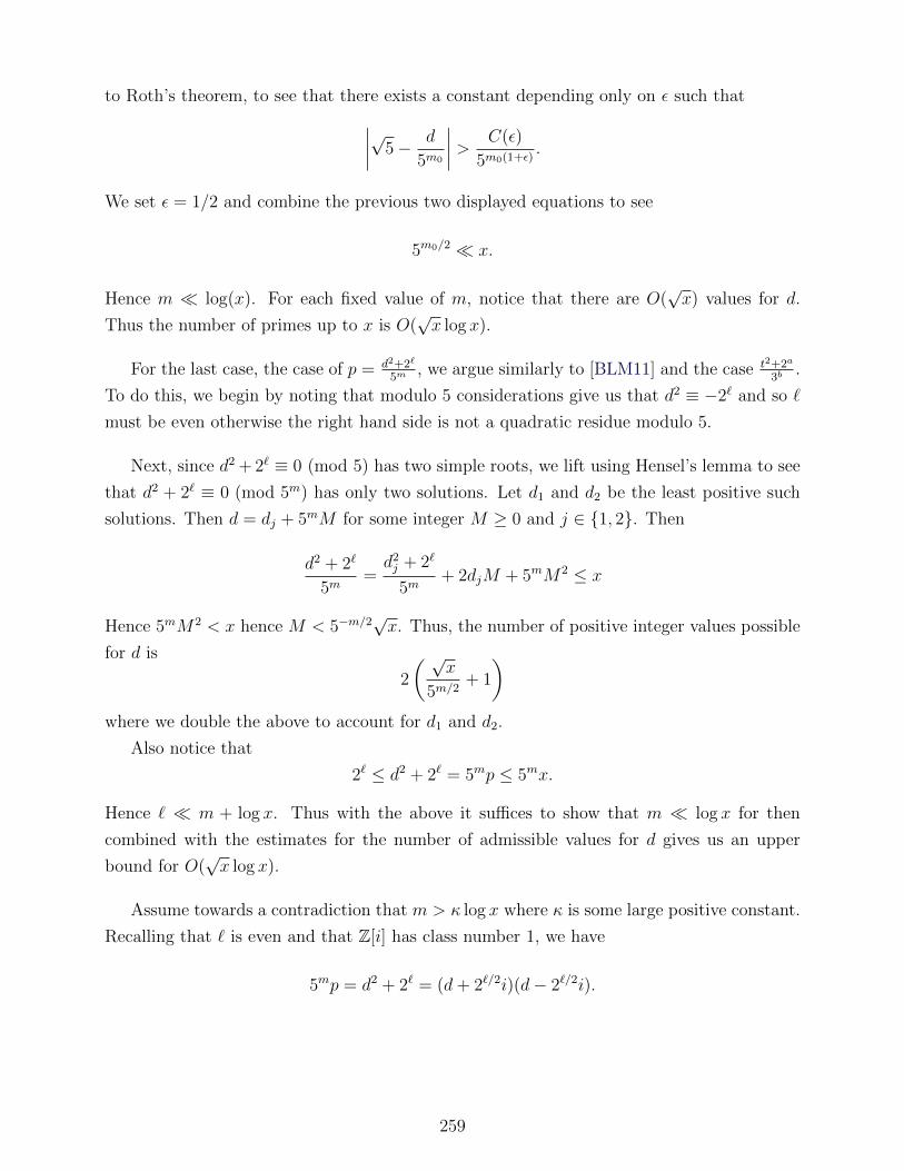
to Roth’s theorem, to see that there exists a constant depending only on ε such that∣∣∣∣√5− d
5m0
∣∣∣∣ > C(ε)
5m0(1+ε).
We set ε = 1/2 and combine the previous two displayed equations to see
5m0/2 x.
Hence m log(x). For each fixed value of m, notice that there are O(√x) values for d.
Thus the number of primes up to x is O(√x log x).
For the last case, the case of p = d2+2`
5m, we argue similarly to [BLM11] and the case t2+2a
3b.
To do this, we begin by noting that modulo 5 considerations give us that d2 ≡ −2` and so `
must be even otherwise the right hand side is not a quadratic residue modulo 5.
Next, since d2 + 2` ≡ 0 (mod 5) has two simple roots, we lift using Hensel’s lemma to see
that d2 + 2` ≡ 0 (mod 5m) has only two solutions. Let d1 and d2 be the least positive such
solutions. Then d = dj + 5mM for some integer M ≥ 0 and j ∈ 1, 2. Then
d2 + 2`
5m=d2j + 2`
5m+ 2djM + 5mM2 ≤ x
Hence 5mM2 < x hence M < 5−m/2√x. Thus, the number of positive integer values possible
for d is
2
( √x
5m/2+ 1
)where we double the above to account for d1 and d2.
Also notice that
2` ≤ d2 + 2` = 5mp ≤ 5mx.
Hence ` m + log x. Thus with the above it suffices to show that m log x for then
combined with the estimates for the number of admissible values for d gives us an upper
bound for O(√x log x).
Assume towards a contradiction that m > κ log x where κ is some large positive constant.
Recalling that ` is even and that Z[i] has class number 1, we have
5mp = d2 + 2` = (d+ 2`/2i)(d− 2`/2i).
259

Thus, we have
d+ 2`/2i = αmp1
d− 2`/2i = αmp1
where α is one of 1± 2i and p1 = u+ vi is such that u2 + v2 = p. Eliminating for d yields
2`/2+1i = αmp1 − αmp1.
Now the 2-adic valuation of the left hand side above is `/2 + 1 and the right hand side has
2-adic valuation of
v2 (αmp1 − αmp1) = v2
((αα
)m p1
p1
− 1
)valid since α and p1 have odd norms. Using [BL96, Theorem 4] a 2-adic linear forms in
logarithms estimate, we see that there exists a constant C such that
v2
((αα
)m p1
p1
− 1
)< C log2
(m
log x
)log x.
Thus, we may conclude that
` < `+1
2< 2C log2
(m
log x
)log x.
Assume towards a contradiction that ` > (log κ)−1m. It follows that
mlog x
log2(
mlog x
) < 2C log κ.
and recalling that we assumed that m > κ log x and that x/ log2 x is an increasing function,
we have
κ < 2C log3 κ.
which is a contradiction if κ is large enough. Hence, we have that ` ≤ (log κ)−1m. This gives
us that
2`/2 ≤ 2m/(2 log κ) ≤ 5m/4 (6.6)
following since 2 log 2log 5
< log κ for sufficiently large κ. We now apply a generalization of the
Schmidt Subspace Theorem due to Schlickewei [Sch77], [Sch91, p.177 Theorem 1D] to the
equation
2`/2+1i = αmp1 − αmp1.
Let K = Q[i] and take a set of valuations to be S = α, α,∞. Let x = (x1, x2). For j = 1, 2
260

and ν ∈ S, take
Lj,ν(x) =
x1 − x2 if (j, ν) = (2,∞)
xj otherwise.
Next, for x = (αmp1, αmp1), we show that
A :=∏
(j,ν)∈1,2×S
|Lj,ν(x)|ν 1
(max|x1, |x2|)1/8. (6.7)
First, compute that ∏ν∈S
|L1,ν(x)|ν = |αmp1|α|αmp1|α|αmp1|
= α−mα−m|αmp1| = |p1|.
Further, ∏ν∈S\∞
|L2,ν(x)|ν = |αmp1|α|αmp1|α = |α−m| = 5−m/2.
Lastly,
|L2,∞(x)| = |x1 − x2| = |αmp1 − αmp1| = 2`/2+1.
Hence from equations 6.6, the product in equation 6.7 becomes
A ≤ |p1|2`/2+1
5m/2≤ 2√x2`/2
5m/2≤ 2√x
5m/4≤ 5−m/8.
where the last inequality holds since m > κ log x and so x < em/κ giving 2√x < 2em/(2κ) ≤
5m/8 provided κ is large enough. This also gives that x ≤ 5m/2 and hence,
|αmp1| = |αmp1| ≤ 5m/2x ≤ 5m.
Combining the above shows that equation 6.7 holds. The Generalized Schmidt Subspace
Theorem [Sch91, p.177 Theorem 1D] asserts that there exists finitely many pairs (ck, dk) ∈K2\(0, 0) for 1 ≤ k ≤ s such that equation 6.6 satisfies ckx1 = dkx2. Without loss of
generality, we may assume that ck and dk are coprime. For a fixed k, this implies that
ckαmp1 = ckx1 = dkx2 = dkα
mp1
which shows that αm | dkαmp1. Since α and α are coprime, we get that αm | dkp1. Since
261

|p1| ≤√p ≤
√x, choosing κ ≥ max1≤k≤s |dk| shows that αm ≤ κ
√x. This will contradict
that m > κ log x. Hence m < κ log x
262

Chapter 7
Strengthening Results on the
Diophantine Equation xq + yq = pαzn
In this section, we will discuss solutions to xq+yq = pαzn for primes not considered above
or in [BLM11]. Let
S3,p = 18p, 36p, 72p C3(p) = p2p
S5,p = 50p, 200p, 400p C5(p) = p13p
and let Sq be the set of primes p ≥ 5 (or p ≥ 7 if q = 5) for which there exists an elliptic
curve E with conductor NE ∈ Sq,p with at least one non-trivial rational two torsion point.
The trick to strengthening the theorem above and the results from [BLM11] is to exploit
more information contained in our Frey-Hellegouarch curve other than the fact that it has
a non-trivial rational two torsion point. Recall that for the curves xq + yq = pαzn with
q ∈ 3, 5, we have the following associated Frey-Hellegouarch curves given by
E3,a,b : y2 = (x+ b− a)(x2 + (a− b)x+ (a2 + ab+ b2)) =: f3(x).
E5,a,b : y2 = x3 − 5(a2 + b2)x2 + 5
(a5 + b5
a+ b
)x
= x
(x2 − 5(a2 + b2)x+ 5
(a5 + b5
a+ b
))=: f5(x).
where (a, b, c) is a solution to xq +yq = pαzn. As notation, we denote by ∆E the discriminant
of the elliptic curve, ∆E,3 the elliptic curve of E3,a,b and ∆E,5 the elliptic curve of E5,a,b and
similarly for ∆E,min to denote the minimal discriminant and NE to denote the conductor for
the elliptic curve E. We make the assumption that if one of a or b is even, we assume without
loss of generality that a is even. This only occurs when c is odd. For the above, we have by
263

[BLM11] and [Bil07] that the invariants are
∆E,3,min = −2433p2αc2n,
NE,3 =
18p · rad6p(c) if c is even, b ≡ −1 (mod 4)
36p · rad6p(c) if c is odd, v2(a) ≥ 2 and b ≡ 1 (mod 4)
72p · rad6p(c) if c is odd, v2(a) = 1 and b ≡ 1 (mod 4),
∆E,5,min = 2453(a+ b)2p2αc2n
NE,5, =
50p · rad10p(c) if c is even, b ≡ −1 (mod 4)
200p · rad10p(c) if c is odd, v2(a) ≥ 2 and b ≡ 1 (mod 4)
400p · rad10p(c) if c is odd, v2(a) = 1 and b ≡ 1 (mod 4).
For curves with a rational two torsion point say y2 = x3 + a2x2 + a4x, let ∆q de-
note the discriminant of the quadratic polynomial x2 + a2x + a4. In the above, let ∆Q,3
be the discriminant of x2 + (a − b)x + (a2 + ab + b2) and let ∆Q,5 be the discriminant of(x2 − 5(a2 + b2)x+ 5
(a5+b5
a+b
)).
Notice that ∆Q,3 = −3(a + b)2 and that ∆Q,5 = 5(a + b)2. Thus, f3(x) splits completely
over F`′ , where `′ is prime, whenever(−3`′
)= 1 and f5(x) splits completely over F`′ whenever(
5`′
)= 1. The first case occurs whenever `′ ≡ 1 (mod 6) and the second occurs whenever
`′ ≡ ±1 (mod 5). Modulo these primes `′, we see that our elliptic curve does not have
full rational two torsion but modulo the primes `′ is pretending to have full rational two
torsion. Mathematically, this means that while #Etor(Q) 6≡ 0 (mod 4) we do have that
#Etor(F`′) ≡ 0 (mod 4) for E being one of E3,a,b or E5,a,b as appropriate. Via Ribet’s Level
Lowering Theorem as in Theorem 1.4.6 (see [BLM11] and [Bil07] for the details) we see that
there is a modular form f of level N where
N =
18p if q = 3, c is even, b ≡ −1 (mod 4)
36p if q = 3, c is odd, v2(a) ≥ 2 and b ≡ 1 (mod 4)
72p if q = 3, c is odd, v2(a) = 1 and b ≡ 1 (mod 4)
50p if q = 5, c is even, b ≡ −1 (mod 4)
200p if q = 5, c is odd, v2(a) ≥ 2 and b ≡ 1 (mod 4)
400p if q = 5, c is odd, v2(a) = 1 and b ≡ 1 (mod 4)
such that a`′(f) ≡ a`′(E) (mod p). Let’s further assume that this f is a rational newform with
nontrivial 2 torsion and a`′(f) 6≡ `+ 1 (mod 4). Then we have that a`′(E) 6≡ a`′(f) (mod 4).
Since at some prime `′ as mentioned above we get that a`′(f) 6= a`′(E), we see via appendice
264

II of [Kra97] that the prime where this difference occurs is small when compared to p2.
This tells us that for such prime p, the equation xq + yq = pαzn has no nontrivial coprime
solutions in integers (x, y, z). After a few more definitions, we can summarize the above work
in a theorem.
Definition 7.0.22. For `′ prime and q ∈ 3, 5, let R(`′, q) be the condition
((−1q )q`′
)= 1.
This is equivalent to(−3`′
)= 1 and
(5`′
)= 1 for q = 3 and q = 5 respectively.
Definition 7.0.23. Let Pg,q denote the set of primes p such that there are no elliptic curves E
with conductor in the set Sq.p such that 4|#ETor(Q) but at least one curve E ′ with conductor
in the same set such that 2|#E ′Tor(Q).
Primes in Pg,3 less than 200 include
53, 79, 83, 103, 149, 151, 157, 163, 167, 173, 181, 199.
and primes in Pg,5 less that 200 include
23, 47, 53, 71, 83, 97, 107, 137, 139, 149, 151, 173, 179, 181, 191, 193, 197.
See the appendix for a longer list.
Note: According to the definition, there needs to be only one curve with conductor in the
set Sq. It could be, for example when q = 3, that you have a curve of conductor 18p with
the required property and no curves with conductor 36p or 72p with 2 | ETor(Q).
Definition 7.0.24. Let Pb,q ⊆ Pg,q be the set of primes p such that p ∈ Pg,q and for every
elliptic curves E with conductor in the set Sq,p such that 2|#ETor(Q), there exists a prime
`′ satisfying both R(`′, q) and a`′(E) 6≡ `′ + 1 (mod 4). Equivalently, there exists a prime `′
satisfying both R(`′, q) and #ETor(F`′) 6≡ 0 (mod 4).
Primes in Pb,3 less than 200 include1
53, 83, 149, 167, 173, 199.
Primes in Pb,5 less that 200 include
23, 53, 71, 73, 83, 97, 107, 137, 151, 173, 181, 191, 193, 197.
Again for longer lists, see the appendix. We now have enough notation to state the main
result of this section.1Note that in [BLM11] paper, the prime 53 listed above was omitted for Pb,3.
265

Theorem 7.0.25. Suppose that q ∈ 3, 5. Suppose that either p ∈ Pb,q ⊆ Sq,p or that
p /∈ Sq,p. Then the equation
xq + yq = pαzn
has no solutions in nonzero, coprime integers x, y and z, integer α ≥ 1 and prime n ≥ Cq(p).
The theorem above tells us that if we can give conditions for primes belonging to Pb,q,then we can show which primes satisfy the above theorem. First, we show which primes do
not belong to Pg,q.
Theorem 7.0.26. Let p be a prime, q ∈ 3.5 and let E : y2 = x3 + a2x2 + a4 be an
elliptic curve with integer coefficients and nontrivial two torsion and conductor in the set
Sq,p. Suppose further that ∆E is a positive square. Then p /∈ Pg,q.
Proof. Notice that the discriminant of x2+a2x+a4 is ∆Q = a22−4a4. Further, the discriminant
of E is
∆E = 16a24(a2
2 − 4a4) = (4a4)2∆Q
Hence, if ∆E is a square, then ∆Q is also a square. Thus, the polynomial x2 + a2x+ a4 splits
over Z. This means that
y2 = x3 + a2x2 + a4x = x(x− α)(x− β)
for some α, β ∈ Z. Hence the curve has full rational two torsion and so p /∈ Pg,q as required.
Now, we display the types of primes that are not in Pg,3 and Pg,5. To form these lists, we
use Theorems 4.0.8, 4.0.10, 4.0.12, 5.0.14, 5.0.16 and 5.0.18 to figure out which cases have the
possibility of having an elliptic curve with square conductor. If there are any present, then
these primes are not members of Pg,q and thus are included below. In all of the tables below,
m ≥ 0 and d ∈ Z unless stated otherwise. The third column throughout we will abbreviate
using the letters TC to mean “Theorem Case”, the entry in the list in the associated theorem.
266

pn Conductor TC Extra Information
2`−2 · 3m + 1 18p 1 n = 1, ` ≥ 7
2`−2 · 3m − 1 18p 2 n = 1, ` ≥ 7
3m + 2`−2 18p 3 n = 1, ` ≥ 7
3m − 2`−2 18p 4 n = 1, ` ≥ 7
2`−2 − 3m 18p 5 n = 1, ` ≥ 7
d2 − 2`3m 18p 7 n = 1, ` ≥ 7 even, m even
2`3m − d2 18p 8 n = 1, ` ≥ 7 even, m evend2+2L
3m18p 9 n = 1, L ≥ 5
2`−2 · 3m + 1 72p 1 n = 1, ` ∈ 4, 52`−2 · 3m − 1 72p 2 n = 1, ` ∈ 4, 5
3m + 2`−2 72p 3 n = 1, ` ∈ 4, 53m − 2`−2 72p 4 n = 1, ` ∈ 4, 5d2 − 2`3m 72p 6 n = 1 or Pmin(n) ≥ 7, ` = 4, m even
2`3m − d2 72p 7 n = 1 or Pmin(n) ≥ 7, ` = 4, m even3m+1
472p 8 n = 1
Table 7.1: Primes not in Pg,3.
267

pn Conductor TC Extra Information
2`−2 · 5m + 1 50p 1 n = 1, ` ≥ 7
2`−2 · 5m − 1 50p 2 n = 1, ` ≥ 72`−2+1
5m50p 3 n = 1, ` ≥ 7
2`−2 − 5m 50p 4 n = 1, ` ≥ 7
5m − 2`−2 50p 5 n = 1, ` ≥ 7
2`−2 + 5m 50p 6 n = 1, ` ≥ 7
d2 − 2`5m 50p 7 n = 1, ` ≥ 7, `,m even
2`5m − d2 50p 8 n = 1, ` ≥ 7, `,m even
2`−2 · 5m + 1 200p 1 n = 1, ` ∈ 4, 52`−2 · 5m − 1 200p 2 n = 1, ` ∈ 4, 5
5m−14
200p 3 n = 1 or Pmin(n) ≥ 7(5m−1
4
)2200p 4 n = 2 or 2 ‖ n and Pmin(n/2) ≥ 7, m odd
5m−d22`
200p 7 Pmin(n) ≥ 7, ` ∈ 2, 4, 5, m even
2`−2 + 5m 200p 8 n = 1 or Pmin(n) ≥ 7, ` ∈ 4, 55m − 2`−2 200p 9 n = 1 and ` ∈ 4, 5 or Pmin(n) ≥ 7 when ` = 4
(5m − 4)2 200p 10 n = 2 or 2 ‖ n and Pmin(n/2) ≥ 7, m odd
d2 − 2`5m 200p 11 n = 1 or Pmin(n) ≥ 7, ` ∈ 2, 4, m even
2`5m − d2 200p 12 n = 1 or Pmin(n) ≥ 7, ` ∈ 2, 4, m even
2`−2 · 5m + 1 400p 1 n = 1, ` ≥ 4
2`−2 · 5m − 1 400p 2 n = 1, ` ≥ 42L+15m
400p 3 n = 1, L ≥ 25m−1
4400p 4 n = 1 or Pmin(n) ≥ 7, m odd
5m−d24
400p 7 n = 1 and m even5m−d2
4400p 8 Pmin(n) ≥ 7, ` ∈ 4, 5
2L + 5m 400p 9 Pmin(n) ≥ 7 and (L+ 2) ∈ 4, 5, n = 1 and L ≥ 2
2L − 5m 400p 10 Pmin(n) ≥ 7 and (L+ 2) ∈ 4, 5, n = 1 and L ≥ 2
5m − 2L 400p 11 Pmin(n) ≥ 7 and L = 2, n = 1 and L ≥ 2
(5m − 4)2 400p 12 n = 2 or 2 ‖ n and Pmin(n/2) ≥ 7, m odd
d2 − 2`5m 400p 13 Either n = 1 and ` ≥ 4 even or both Pmin(n) ≥ 7 and
` ∈ 2, 4, m even
2`5m − d2 400p 14 Either n = 1 and ` ≥ 4 even or both Pmin(n) ≥ 7 and
` ∈ 2, 4, m evend2+45m
400p 16 n = 2 or 2 ‖ n and Pmin(n/2) ≥ 7, m even
Table 7.2: Primes not in Pg,5.
At first, the goal to classify primes in Pg,q but not in Pb,q is much easier. In fact, we have
268

the following.
Theorem 7.0.27. Let q ∈ 3, 5. Let p ∈ Pg,q and let E/Q be an elliptic curve with
conductor in Sq,p with rational two torsion. Suppose further that the discriminant of the
elliptic curve is of the form
∆E =
(−3)m2 if q = 3
5m2 if q = 5
for some integer m. Then p /∈ Pb,q.
Proof. By shifting the rational two torsion point to (0, 0), the curve E can be seen to be
isomorphic to a curve of the form
y2 = x3 + a2x2 + a4x = x(x2 + a2x+ a4)
so without loss of generality, suppose E is of this form. According to [Sil09, p.42], we have
that
∆E = 16a24(a2
2 − 4a4) = (4a4)2∆Q
where ∆Q is the discriminant of the quadratic polynomial x2 + a2x + a4. By assumption
∆E = ∆Q,q and so in fact, we have that
∆Q =∆E
(4a4)2=
(−3)n2 if q = 3
5n2 if q = 5
where (4a4n)2 = m2. Let ∆Q,q,n represent the right most side of the above equality.
Assume towards a contradiction that p ∈ Pb,q. Then there exists a prime2 `′ 6= p satisfying
R(`′, q) such that 4 - #ETor(F`′). However, in this case, we know that ∆Q = ∆Q,q,n. But for
such `′, we have that the Legendre symbol evaluates to(∆Q,q,n
`′
)= 1 by definition of R(`′, q).
Thus, ∆Q is a square in F`′ . Hence, the polynomial x2 + a2x+ a4 splits and thus
y2 = x3 + a2x2 + a4x = x(x2 + a2x+ a4) = x(x− α)(x− β)
where α, β ∈ F`′ . Hence, we have that the curve has full rational two torsion over F`′ and so
we have that 4|#ETor(F`′) which is a contradiction. Thus p /∈ Pb,q as was required.
Now, we can list the families with discriminant of the form −3m2. Hence a prime p that
lives in these families and belongs to Pg,q does not belong to Pb,q. I summarize these families
in the following table. As before, m ≥ 0 and d ∈ Z unless otherwise indicated.
2we need to avoid the conductor for reduction purposes so ensure that `′ 6= p.
269

pn Conductor TC Extra Information
d2 + 2`3m 18p 6 n = 1, ` ≥ 7 even, m odd
3d2 + 2` 18p 10 n = 1, ` ≥ 7 evend2+3m
436p 4 n = 1, p ≡ −1 (mod 4), m odd
3d2+14
36p 5 n ∈ 1, 2, p ≡ 1 (mod 4)
d2 + 2`3m 72p 5 n = 1, ` ∈ 2, 4, m odd3m+d2
472p 9 n = 1, p ≡ 1 (mod 4), m odd
3d2+14
72p 10 n ∈ 1, 23d2 + 2` 72p 13 n = 1, ` ∈ 2, 4
Table 7.3: Primes not in Pb,3 but in Pg,3.
270

pn Conductor TC Extra Information
d2 − 2`5m 50p 7 n = 1, ` ≥ 7 even, m odd
2`5m − d2 50p 8 n = 1, ` ≥ 7 even, m odd
5d2 − 2` 50p 10 n = 1, ` ≥ 7 even
2` − 5d2 50p 11 n = 1, ` ≥ 7 evend2−5m
4200p 5 n = 1 or Pmin(n) ≥ 7, m odd
5m−d24
200p 6 n = 1 or Pmin(n) ≥ 7, m odd5m−d2
2`200p 7 Pmin(n) ≥ 7, ` ∈ 2, 4, 5 m odd
d2 − 2`5m 200p 11 n = 1 or Pmin(n) ≥ 7, ` ∈ 2, 4, m odd
2`5m − d2 200p 12 n = 1 or Pmin(n) ≥ 7, ` ∈ 2, 4, m odd5d2−1
4200p 15 n = 1 or n = 2 or Pmin(n) ≥ 7 or 2 ‖ n and Pmin(n/2) ≥
7, pn ≡ 1 (mod 4)
5d2 − 2` 200p 16 n = 1 or Pmin(n) ≥ 7 and ` ∈ 2, 4(5m−1
4
)2400p 5 n = 2 or 2 ‖ n and Pmin(n/2) ≥ 7, m odd
d2−5m
4400p 6 n = 1 or Pmin(n) ≥ 7, m odd
5m−d24
400p 7 n = 1 or Pmin(n) ≥ 7, m odd
d2 − 2`5m 400p 13 Either n = 1 and ` ≥ 4 even or Pmin(n) ≥ 7 and ` ∈2, 4, m odd
2`5m − d2 400p 14 Either n = 1 and ` ≥ 2 even or Pmin(n) ≥ 7 and ` ∈2, 4, m odd
d2+45m
400p 16 n = 2 or 2 ‖ n and Pmin(n/2) ≥ 7, m odd5d2−1
4400p 17 n = 1 or n = 2 or Pmin(n) ≥ 7 or 2 ‖ n and Pmin(n/2) ≥
7, pn ≡ 1 (mod 4)
5d2 − 2` 400p 18 One of n = 1 and ` ≥ 2 even, Pmin(n) ≥ 7 and ` ∈ 2, 4,n = 2 or 2 ‖ n and Pmin(n/2) ≥ 7 and ` = 2
2` − 5d2 400p 19 n = 1, ` ≥ 4 even
5d2 + 4 400p 20 n = 2 or 2 ‖ n and Pmin(n/2) ≥ 7
Table 7.4: Primes not in Pb,5 but in Pg,5.
This leaves the following primes. Below we let m ≥ 0, d > 0 be integers and s ∈ 0, 1unless otherwise specified.
271

pn Conductor TC Extra Information a4 Legendre for a4 ∆ Legendre for ∆d2 + 2`3m 18p 6 n = 1,` ≥ 7, either ` odd or
both `,m even−2`−23m+2
(−2·3`′
)or(−2`′
)or(−1`′
)22`32m+6p
(p`′
)d2 − 2`3m 18p 7 n = 1,` ≥ 7, either ` odd or
m odd2`−23m+2
(2·3`′
)or(
2`′
)or(
3`′
)22`32m+6p
(p`′
)2`3m − d2 18p 8 n = 1,` ≥ 7, either ` odd or
m odd2`−23m+2
(2·3`′
)or(
2`′
)or(
3`′
)−22`32m+6p
(−p`′
)3d2 + 2` 18p 10 n = 1,` ≥ 7 odd −2`−232s+1
(−2·3`′
)22`36s+3p
(3p`′
)3d2 − 2` 18p 11 n = 1,` ≥ 7 2`−232s+1
(3`′
)or(
2·3`′
)22`36s+3p
(3p`′
)2` − 3d2 18p 12 n = 1,` ≥ 7 2`−232s+1
(3`′
)or(
2·3`′
)−22`36s+3p
(−3p`′
)d2 + 4 · 3m 36p 1 n = 1,m even −3m+2
(−1`′
)2432m+6p
(p`′
)d2 − 4 · 3m 36p 2 n = 1 or Pmin(n) ≥ 7,m odd −3m+2
(3`′
)2432m+6pn
(p`′
)4 · 3m − d2 36p 3 n = 1 or Pmin(n) ≥ 7,m odd −3m+2
(3`′
)−2432m+6pn
(−p`′
)3d2 − 4 36p 6 n = 1 32s+1
(3`′
)2436s+3p
(3p`′
)d2 + 2`3m 72p 5 n = 1, either both ` ∈ 2, 4
and m even or just ` = 5−2`−23m+2
(−1`′
)or(−2`′
)or(−2·3
`′
)22`32m+6p
(p`′
)d2 − 2`3m 72p 6 n = 1 or Pmin(n) ≥ 7, either
both ` = 4 and m even orjust ` = 5
2`−23m+2(
2`′
)or(
2·3`′
)or(
3`′
)22`32m+6pn
(p`′
)2`3m − d2 72p 7 n = 1 or Pmin(n) ≥ 7, either
both ` = 4 and m even orjust ` = 5
2`−23m+2(
2`′
)or(
2·3`′
)or(
3`′
)−22`32m+6pn
(−p`′
)d2+32
3m72p 11 n = 1 or Pmin(n) ≥ 7 −233m+2
(−2`′
)2103m+6pn
(p`′
)or(
3p`′
)3d2 − 2` 72p 12 n = 1, ` ∈ 4, 5 2`−232s+1
(2·3`′
)or(
3`′
)22`36s+3p
(3p`′
)3d2 + 32 72p 13 n = 1 −2332s+1
(−2·3`′
)21036s+3p
(3p`′
)Table 7.5: Remaining primes for q = 3.
272

pn Conductor TC Extra Information a4 Legendre for a4 ∆ Legendre for ∆d2 − 2`5m 50p 7 n = 1,` ≥ 7 odd 2`−25m+2
(2·5`′
)or(
2`′
)22`52m+6p
(p`′
)2`5m − d2 50p 8 n = 1,` ≥ 7 odd 2`−25m+2
(2·5`′
)or(
2`′
)−22`52m+6p
(−p`′
)d2 + 2`5m 50p 9 n = 1,` ≥ 7 −2`−25m+2
(−2·5`′
)or(−2`′
)or(−5`′
)22`52m+6p
(p`′
)5d2 − 2` 50p 10 n = 1,` ≥ 7 odd 2`−252s+1
(2·5`′
)22`56s+3p
(5p`′
)2` − 5d2 50p 11 n = 1,` ≥ 7 odd 2`−252s+1
(2·5`′
)−22`56s+3p
(−5p`′
)5d2 + 2` 50p 12 n = 1,` ≥ 7 −2`−252s+1
(−2·5`′
)or(−5`′
)22`56s+3p
(5p`′
)d2 − 32 · 5m 200p 11 n = 1 or Pmin(n) ≥ 7 235m+2
(2`′
)or(
2·5`′
)22`52m+6pn
(p`′
)32 · 5m − d2 200p 12 n = 1 or Pmin(n) ≥ 7 235m+2
(2`′
)or(
2·5`′
)−22`52m+6pn
(−p`′
)d2 + 2`5m 200p 13 n = 1, ` ∈ 2, 4, 5 −2`−25m+2
(−5`′
)or(−2·5
`′
)22`52m+6p
(p`′
)d2+16
5m200p 14 n = 1 or Pmin(n) ≥ 7 −223m+2
(−1`′
)285m+6pn
(p`′
)or(
5p`′
)5d2 − 32 200p 16 n = 1 or Pmin(n) ≥ 7 2352s+1
(2·5`′
)21056s+3pn
(5p`′
)5d2 + 2` 200p 17 n = 1 or Pmin(n) ≥ 7 −2`−252s+1
(−2·5`′
)or(−5`′
)22`56s+3p
(5p`′
)d2 − 2`5m 400p 13 n = 1 and ` ≥ 5 odd or both
Pmin(n) ≥ 7 and ` = 52`−25m+2
(2·5`′
)or(
2`′
)22`52m+6pn
(p`′
)2`5m − d2 400p 14 n = 1 and ` ≥ 5 odd or both
Pmin(n) ≥ 7 and ` = 52`−25m+2
(2·5`′
)or(
2`′
)−22`52m+6p
(−p`′
)d2 + 2`5m 400p 15 n = 1, either both m = 0 −2`−25m+2
(−2·5`′
)or(−2`′
)22`52m+6p
(p`′
)and ` = 2 or ` ≥ 4 or
(−5`′
)or(−1`′
)d2+2`
5m400p 16 n = 1 or Pmin(n) ≥ 7 and
` ∈ 2, 4, or n = 1 and ` ≥5
−2`−252(
2·5`′
)or(−1`′
)22`5m+6pn
(5p`′
)or(p`′
)5d2 − 2` 400p 18 n = 1 and ` ≥ 5 odd, or
Pmin(n) ≥ 7 and ` = 52`−252s+1
(2·5`′
)22`56s+3pn
(5p`′
)2` − 5d2 400p 19 n = 1,` ≥ 5 odd 2`−252s+1
(2·5`′
)−22`56s+3p
(−5p`′
)5d2 + 2` 400p 20 n = 1 or Pmin(n) ≥ 7 and
` ∈ 2, 4, 5, or n = 1 and` ≥ 6
−2`−252s+1(−2·5
`′
)or(−5`′
)22`56s+3p
(5p`′
)
Table 7.6: Remaining primes for q = 5.
273

In fact, the data suggest that the converse is also true, that is, primes that are not in
tables 7.3 and 7.1 (thus, ones that are in 7.5) are in Pb,3 and similarly, primes that are not in
tables 7.4 and 7.2 (thus, ones that are in 7.6) are in Pb,5 . One has to be a bit careful though
with the argument as the following example illustrates.
Example 7.0.28. Suppose q = 3 and consider the curves in the isogeny class 25902a. As
25902 = (18)(1439) and 1439 = 215 − (177)2, we have that this curve belongs to Theorem
4.0.8 case 8 with t = 177, a = 15 and b = 0. Thus, we have that our curve is isogenous to
say
y2 = x3 − 3(177)x2 + 21332x
with discriminant ∆ = −23036(1439). This discriminant is not of the form (−3)m2 and so
there should be a prime `′ so that 4 - #ETor(Q). Notice that ` = 7 is a prime such that(−14397
)= −1 and so the polynomial does not split in F7. However, the above elliptic curve
over F7 has torsion subgroup of order 4. What has happened here is that over F7 even though
we do not get splitting, we have that the torsion subgroup has gone from a group isomorphic
to Z/2Z to a group isomorphic to Z/4Z. As it turns out, the smallest prime that shows that
1439 ∈ Pb is actually ` = 139 where the torsion subgroup of the curve over F139 is isomorphic
to Z/162Z.
Lemma 7.0.29. Let q ∈ 3, 5. Let a ∈ 2, 3, m = 2aq and b ∈ (Z/mZ)×. For every
prime p ≥ 3 distinct from q and δ, ε ∈ ±1, there exists a prime `′ such that(δp`′
)= ε and
`′ ≡ b (mod m).
Proof. Notice that
ε =
(δp
`′
)= (δ)
`′−12
(p
`′
)= (δ)
`′−12 (−1)
p−12
`′−12
(`′
p
).
By multiplying both sides by (δ)`′−1
2 (−1)p−1
2`′−1
2 , we see that we are then reduced to finding
an `′ so that (`′
p
)= ε(δ)
`′−12 (−1)
p−12
`′−12
If `′ ≡ 1 (mod 4) is consistent with `′ ≡ b (mod m), then notice that the right hand side
is just ε. Alternatively, if `′ ≡ 3 (mod 4), then the right hand side becomes ±εδ where the
± sign is determined by p ≡ ±1 (mod 4). In either case, we need to find a value of `′ such
that(`′
p
)= ±1. If we want
(`′
p
)= −1, choose an integer d such that
(dp
)= −1. Such an d
must exist since the Legendre symbol is a nontrivial real character when p ≥ 3. If we want(`′
p
)= 1, then we can choose d = 1 and notice that
(dp
)= 1. Now via the Chinese Remainder
Theorem, find a simultaneous solution, say `0 such that
`0 ≡ d 6≡ 0 (mod p) and `0 ≡ b 6≡ 0 (mod m).
274

The Chinese Remainder Theorem also gives that all solutions are given by `′ ≡ `0 (mod pm).
As gcd(`0, pm) = 1, by Dirichlet’s Theorem for Primes in an Arithmetic Progression, we have
that there exists a prime `′ such that `′ ≡ `0 (mod pm). This completes the proof.
Now we prove the main theorem.
Theorem 7.0.30. Let q ∈ 3, 5 and let p ∈ Pg,q. Then p ∈ Pb,q if and only if every elliptic
curve with conductor in Sq,p with non-trivial rational two torsion has discriminant not of the
form ∆Q,q,m :=(−1q
)qm2 for all integers m.
Proof. The reverse direction was Theorem 7.0.27 so it suffices to show the forward direction.
Notice that there are only two cases where p /∈ Pb,q.
1. The polynomial x3 + a2x2 + a4x associated to our elliptic curve splits modulo every
prime `′ ≡ 1 (mod 6).
2. For every prime `′ ≡ 1 (mod 6), there exists a point P on our elliptic curve such that
P 6= (0, 0) but 2P = (0, 0).
Hence, we need to show that for each curve avoiding discriminants of the form(−1q
)qm2, we
can find a prime ` satisfying R(`′, q) where the curve does not split and that there is no point
P as specified above. To show this, notice that the duplication formula [ST92, p. 31] for
curves of the form E : y2 = x3 + a2x2 + a4x says that if P = (x, y) is a point on E, then
x(2P ) =x4 − 2a4x
2 + a24
4y2=
(x2 − a4)2
4y2.
According to the duplication formula, the second condition above can occur for a prime `′
only if (x2 − a4)2 ≡ 0 (mod `′) and so we must have that a4 is a quadratic residue modulo
`′ for every prime `′ ≡ 1 (mod 6) if our theorem is to be false. Thus, for every curve in our
families from Theorems 4.0.8, 4.0.10, 4.0.12, 5.0.14, 5.0.16 and 5.0.18, we must show that we
can find a prime `′ so that
1.(
∆`′
)= −1
2.(a4`′
)= −1
3.((−1
q )qm2
`′
)=((−1
q )q`′
)= 1 or equivalently R(`′, q) holds.
All that’s left to do is show that this is possible for each curve in the list with the exception
of the two forbidden families we have already discarded. We look at Tables 7.5 and 7.6. In
those tables, the a4 and ∆ values correspond to the first curve in each case. Choosing other
curves in the family will flip the roles of ∆ and a4 so we reduce our argument to just looking
at the table given.
275

Notice that in the tables, the Legendre symbol for ∆ never contains a 2. Thus the value(∆`′
)is always of the form
(±pq`′
)or(±p`′
). Since R(`′, q) holds, we can multiply the case of(±pq
`′
)= −1 by the condition
((−1q )q`′
)= 1 on both sides to see that the condition
(∆`′
)= −1 is
always of the form(±p`′
)= −1.
As for a4, using the tables, we see that(a4`′
), up to multiplication by
((−1q )q`′
)= 1 is one
of the following cases:
1.(−1`′
)2.(±2`′
)Next, recall that R(`′, 3) is the condition that `′ ≡ 1 (mod 6) which splits into the con-
ditions that `′ ≡ 1 (mod 2) and `′ ≡ 1 (mod 3). The first condition tells us that `′ is odd
and this is consistent with the first three cases above. Recall also that(−1`′
)and
(±2`′
)each
impose conditions on the prime `′ modulo 8. Thus, combining these gives us that either
`′ ≡ k (mod 8) and one of `′ ≡ 1 (mod 3) or `′ ≡ ±1 (mod 5) . The Chinese Remainder
Theorem puts us in the situation as needed in Lemma 7.0.29 which gives us an admissible
prime `′. This completes the proof.
This gives the following theorem
Theorem 7.0.31. Let q ∈ 3, 5 and suppose that p is a prime such that p 6∈ Sq or that
p ∈ Pb,q ⊆ Sq. Then the equation xq + yq = pαzn has no nontrivial coprime integer solutions
(x, y, z) where α ≥ 1 and n ≥ Cq(p) a prime. Furthermore, if the prime p avoids the lists in
Tables 7.1 and 7.3 (hence residing in Table 7.5) when q = 3 or in Tables 7.2 and 7.4 (hence
residing in Table 7.6) when q = 5, then we have that p 6∈ Sq or that p ∈ Pb,q ⊆ Sq.
Some final comments. To what end can this technique be extended? Can we try to solve
the Diophantine equation x7 + y7 = pαzn? Suppose that a7 + b7 = pαcn is a given solution.
In this case, the only known Frey curve is given by
y2 = x3 − (a− b)2x2 + (−2a4 + ba3 − 5b2a2 + b3a− 2b4)x
+ a6 − 6ba5 + 8b2a4 − 13b3a3 + 8b4a2 − 65a+ b6
with discriminant
∆ = 2472
(a7 + b7
a+ b
)2
.
This curve does not have rational two torsion, which was a crucial ingredient for this technique
to work. A natural place to perhaps use this technique would be over Q-curves, that is, elliptic
276

curves over some number field that are isogenous to its Galois conjugates. An example of this
curve is the one associated to a solution (a, b, c) to the Diophantine equation x2 + y4 = zn
given by
y2 = x3 + 2(1 + i)bx2 + i(b2 + ia)x.
There is a possibility that the techniques above could all extend over to the equation x2+y4 =
pαzn though I have not attempted to adapt the above to elliptic curves over Q(i). Here with
units being ±1 and ±i, the techniques used in [Mul06] have a chance of carrying over. There
is also potential for this technique to work with Hilbert modularity forms extending the recent
work of [Fre10] though much of the work would need to be substantially revised to work over
arbitrary totally real fields instead of over Q. Work in this direction is still relatively new
and there is much hope that modifications of the above will lead to fruitful mathematical
research in the upcoming years.
277
Bibliography
[AAA02] S. A. Arif and A. S. Al-Ali. On the Diophantine equation x2 + p2k+1 = 4yn. Int.
J. Math. Math. Sci., 31(11):695–699, 2002.
[AAM01] S. A. Arif and F. S. Abu Muriefah. On the Diophantine equation x2 + 2k = yn.
II. Arab J. Math. Sci., 7(2):67–71, 2001.
[Ahl66] L. V. Ahlfors. Complex analysis: An introduction of the theory of analytic
functions of one complex variable. Second edition. McGraw-Hill Book Co., New
York, 1966.
[Akh09] S. Akhtari. The Diophantine equation aX4 − bY 2 = 1. J. Reine Angew. Math.,
630:33–57, 2009.
[AMLST09] F. S. Abu Muriefah, F. Luca, S. Siksek, and S. Tengely. On the Diophantine
equation x2 + C = 2yn. Int. J. Number Theory, 5(6):1117–1128, 2009.
[Bak67] A. Baker. Linear forms in the logarithms of algebraic numbers. I, II, III. Math-
ematika 13 (1966), 204-216; ibid. 14 (1967), 102-107; ibid., 14:220–228, 1967.
[Bak68] A. Baker. Linear forms in the logarithms of algebraic numbers. IV. Mathematika,
15:204–216, 1968.
[Bal60] W. W. R. Ball. A short account of the history of mathematics. Dover Publica-
tions Inc., New York, 1960.
[BC06] W. Bosma and J. Cannon, editors. Discovering mathematics with Magma, vol-
ume 19 of Algorithms and Computation in Mathematics. Springer-Verlag, Berlin,
2006. Reducing the abstract to the concrete.
[BCDT01] C. Breuil, B. Conrad, F. Diamond, and R. Taylor. On the modularity of ellip-
tic curves over Q: wild 3-adic exercises. J. Amer. Math. Soc., 14(4):843–939
(electronic), 2001.
[BCDY14] M. A. Bennett, I. Chen, S. R. Dahmen, and S. Yazdani. On the equation
a3 + b3n = c2. Acta Arith., 163(4):327–343, 2014.
278

[BCP97] W. Bosma, J. Cannon, and C. Playoust. The Magma algebra system. I. The user
language. J. Symbolic Comput., 24(3-4):235–265, 1997. Computational algebra
and number theory (London, 1993).
[BD10] N. Billerey and L. V. Dieulefait. Solving Fermat-type equations x5 + y5 = dzp.
Math. Comp., 79(269):535–544, 2010.
[Bil07] N. Billerey. Equations de Fermat de type (5, 5, p). Bull. Austral. Math. Soc.,
76(2):161–194, 2007.
[BK94] A. Brumer and K. Kramer. The conductor of an abelian variety. Compositio
Math., 92(2):227–248, 1994.
[BL96] Y. Bugeaud and M. Laurent. Minoration effective de la distance p-adique entre
puissances de nombres algebriques. J. Number Theory, 61(2):311–342, 1996.
[BLM11] M. A. Bennett, F. Luca, and J. Mulholland. Twisted extensions of the cubic
case of Fermat’s last theorem. Ann. Sci. Math. Quebec, 35(1):1–15, 2011.
[BMS+08] Y. Bugeaud, M. Mignotte, S. Siksek, Michael Stoll, and Szabolcs Tengely. In-
tegral points on hyperelliptic curves. Algebra Number Theory, 2(8):859–885,
2008.
[Bru00] Nils Bruin. On powers as sums of two cubes. In Algorithmic number theory
(Leiden, 2000), volume 1838 of Lecture Notes in Comput. Sci., pages 169–184.
Springer, Berlin, 2000.
[Bru02] N. R. Bruin. Chabauty methods and covering techniques applied to generalized
Fermat equations, volume 133 of CWI Tract. Stichting Mathematisch Centrum,
Centrum voor Wiskunde en Informatica, Amsterdam, 2002. Dissertation, Uni-
versity of Leiden, Leiden, 1999.
[Bru03] N. Bruin. Chabauty methods using elliptic curves. J. Reine Angew. Math.,
562:27–49, 2003.
[BS66] A. I. Borevich and I. R. Shafarevich. Number theory. Translated from the Rus-
sian by Newcomb Greenleaf. Pure and Applied Mathematics, Vol. 20. Academic
Press, New York, 1966.
[BS04] M. A. Bennett and C. M. Skinner. Ternary Diophantine equations via Galois
representations and modular forms. Canad. J. Math., 56(1):23–54, 2004.
[BS08] N. Bruin and M. Stoll. Deciding existence of rational points on curves: an
experiment. Experiment. Math., 17(2):181–189, 2008.
279

[BS09] N. Bruin and M. Stoll. Two-cover descent on hyperelliptic curves. Math. Comp.,
78(268):2347–2370, 2009.
[BS10] N. Bruin and M. Stoll. The Mordell-Weil sieve: proving non-existence of rational
points on curves. LMS J. Comput. Math., 13:272–306, 2010.
[BVY04] M. A. Bennett, V. Vatsal, and S. Yazdani. Ternary Diophantine equations of
signature (p, p, 3). Compos. Math., 140(6):1399–1416, 2004.
[CF96] J. W. S. Cassels and E. V. Flynn. Prolegomena to a middlebrow arithmetic of
curves of genus 2, volume 230 of London Mathematical Society Lecture Note
Series. Cambridge University Press, Cambridge, 1996.
[Cha41] C. Chabauty. Sur les points rationnels des courbes algebriques de genre superieur
a l’unite. C. R. Acad. Sci. Paris, 212:882–885, 1941.
[Coh91] J. H. E. Cohn. The Diophantine equations x3 = Ny2 ± 1. Quart. J. Math.
Oxford Ser. (2), 42(165):27–30, 1991.
[Coh92] J. H. E. Cohn. The Diophantine equation x2 + 2k = yn. Arch. Math. (Basel),
59(4):341–344, 1992.
[Coh96] J. H. E. Cohn. Perfect Pell powers. Glasgow Math. J., 38(1):19–20, 1996.
[Coh97] J. H. E. Cohn. The Diophantine equation x4 − Dy2 = 1. II. Acta Arith.,
78(4):401–403, 1997.
[Coh03] J. H. E. Cohn. The Diophantine equation x2 + C = yn. II. Acta Arith.,
109(2):205–206, 2003.
[Coh07a] H. Cohen. Number theory. Vol. I. Tools and Diophantine equations, volume 239
of Graduate Texts in Mathematics. Springer, New York, 2007.
[Coh07b] H. Cohen. Number theory. Vol. II. Analytic and modern tools, volume 240 of
Graduate Texts in Mathematics. Springer, New York, 2007.
[Col85] R. F. Coleman. Effective Chabauty. Duke Math. J., 52(3):765–770, 1985.
[Cre] J. Cremona. Elliptic curve data. http://homepages.warwick.ac.uk/~masgaj/
ftp/data/, visited 2015-01-26.
[Cre97] J. E. Cremona. Algorithms for modular elliptic curves. Cambridge University
Press, Cambridge, second edition, 1997.
280

[CS09] Imin Chen and Samir Siksek. Perfect powers expressible as sums of two cubes.
J. Algebra, 322(3):638–656, 2009.
[Dah08] S. R. Dahmen. Classical and modular methods applied to Diophantine equations.
2008. Utrecht University, Ph.D. thesis.
[Dav95] S. David. Minorations de formes lineaires de logarithmes elliptiques. Mem. Soc.
Math. France (N.S.), (62):iv+143, 1995.
[Del74] P. Deligne. La conjecture de Weil. I. Inst. Hautes Etudes Sci. Publ. Math.,
(43):273–307, 1974.
[Del80] P. Deligne. La conjecture de Weil. II. Inst. Hautes Etudes Sci. Publ. Math.,
(52):137–252, 1980.
[Den52] P. Denes. Uber die Diophantische Gleichung xl + yl = czl. Acta Math., 88:241–
251, 1952.
[Dev90] K. Devlin. Mathematics: the new Golden Age. Penguin Books, New York, 1990.
[DF04] D. S. Dummit and R. M. Foote. Abstract algebra. John Wiley & Sons Inc.,
Hoboken, NJ, third edition, 2004.
[DG95] H. Darmon and A. Granville. On the equations zm = F (x, y) and Axp +Byq =
Czr. Bull. London Math. Soc., 27(6):513–543, 1995.
[DK95] Fred Diamond and Kenneth Kramer. Modularity of a family of elliptic curves.
Math. Res. Lett., 2(3):299–304, 1995.
[DM97] H. Darmon and L. Merel. Winding quotients and some variants of Fermat’s last
theorem. J. Reine Angew. Math., 490:81–100, 1997.
[DR11] V. Dragovic and M. Radnovic. Poncelet porisms and beyond. Frontiers in Math-
ematics. Birkhauser/Springer Basel AG, Basel, 2011. Integrable billiards, hy-
perelliptic Jacobians and pencils of quadrics.
[DS05] F. Diamond and J. Shurman. A first course in modular forms, volume 228 of
Graduate Texts in Mathematics. Springer-Verlag, New York, 2005.
[dW89] B. M. M. de Weger. Algorithms for Diophantine equations, volume 65 of CWI
Tract. Stichting Mathematisch Centrum, Centrum voor Wiskunde en Informat-
ica, Amsterdam, 1989.
[Ell04] J. S. Ellenberg. Galois representations attached to Q-curves and the generalized
Fermat equation A4 +B2 = Cp. Amer. J. Math., 126(4):763–787, 2004.
281
[Euc02] Euclid. Euclid’s Elements. Green Lion Press, Santa Fe, NM, 2002. All thirteen
books complete in one volume, The Thomas L. Heath translation, Edited by
Dana Densmore.
[Fal83] G. Faltings. Endlichkeitssatze fur abelsche Varietaten uber Zahlkorpern. Invent.
Math., 73(3):349–366, 1983.
[Fre86] G. Frey. Links between stable elliptic curves and certain Diophantine equations.
Ann. Univ. Sarav. Ser. Math., 1(1):iv+40, 1986.
[Fre09] G. Frey. The way to the proof of Fermat’s last theorem. Ann. Fac. Sci. Toulouse
Math. (6), 18(Fascicule Special):5–23, 2009.
[Fre10] N. R. B. Freitas. Some Generalized Fermat-Type Equations via Q-curves and
Modularity. 2010. Thesis (Ph.D.)–Universitat de Barcelona (Spain).
[GLT08] E. Goins, F. Luca, and A. Togbe. On the Diophantine equation x2 + 2α5β13γ =
yn. In Algorithmic number theory, volume 5011 of Lecture Notes in Comput.
Sci., pages 430–442. Springer, Berlin, 2008.
[GR11] H. R. Gallegos-Ruiz. S-integral points on hyperelliptic curves. Int. J. Number
Theory, 7(3):803–824, 2011.
[Ham11] K. D. Hambrook. Implementaiton of a Thue-Mahler Equation Solver. 2011.
Thesis (M.Sc.)–The University of British Columbia (Canada).
[Hel75] Y. Hellegouarch. Points d’ordre 2ph sur les courbes elliptiques. Acta Arith.,
26(3):253–263, 1974/75.
[HK98] E. Halberstadt and A. Kraus. Sur les modules de torsion des courbes elliptiques.
Math. Ann., 310(1):47–54, 1998.
[HPPT13] B. He, I. Pink, A. Pinter, and A. Togbe. On the Diophantine inequality |X2 −cXY 2 + Y 4| ≤ c+ 2. Glas. Mat. Ser. III, 48(68)(2):291–299, 2013.
[HS00] M. Hindry and J. H. Silverman. Diophantine geometry, volume 201 of Graduate
Texts in Mathematics. Springer-Verlag, New York, 2000. An introduction.
[Ito87] K. Ito, editor. Encyclopedic dictionary of mathematics. Vol. I–IV. MIT Press,
Cambridge, MA, second edition, 1987. Translated from the Japanese.
[Ivo04] W. Ivorra. Equations diophantiennes ternaires de type (p,p,2) et courbes ellip-
tiques. 2004. Thesis (Ph.D.)– Universite Pierre et Marie Curie.
282

[Ken82] M. A. Kenku. On the number of Q-isomorphism classes of elliptic curves in each
Q-isogeny class. J. Number Theory, 15(2):199–202, 1982.
[Kna92] A. W. Knapp. Elliptic curves, volume 40 of Mathematical Notes. Princeton
University Press, Princeton, NJ, 1992.
[KO92] A. Kraus and J. Oesterle. Sur une question de B. Mazur. Math. Ann.,
293(2):259–275, 1992.
[Kra97] A. Kraus. Majorations effectives pour l’equation de Fermat generalisee. Canad.
J. Math., 49(6):1139–1161, 1997.
[Kra98] A. Kraus. Sur l’equation a3 + b3 = cp. Experiment. Math., 7(1):1–13, 1998.
[Kra99] A. Kraus. On the equation xp+yq = zr: a survey. Ramanujan J., 3(3):315–333,
1999.
[KW09a] C. Khare and J.-P. Wintenberger. Serre’s modularity conjecture. I. Invent.
Math., 178(3):485–504, 2009.
[KW09b] C. Khare and J.-P. Wintenberger. Serre’s modularity conjecture. II. Invent.
Math., 178(3):505–586, 2009.
[Lju42] W. Ljunggren. Uber die Gleichung x4 − Dy2 = 1. Arch. Math. Naturvid.,
45(5):61–70, 1942.
[Lju54] W. Ljunggren. Ein Satz uber die diophantische Gleichung Ax2−By4 = C (C =
1, 2, 4). In Tolfte Skandinaviska Matematikerkongressen, Lund, 1953, pages 188–
194. Lunds Universitets Matematiska Inst., Lund, 1954.
[Lju67] W. Ljunggren. On the diophantine equation Ax4 −By2 = C (C = 1, 4). Math.
Scand., 21:149–158 (1969), 1967.
[LLL82] A. K. Lenstra, H. W. Lenstra, Jr., and L. Lovasz. Factoring polynomials with
rational coefficients. Math. Ann., 261(4):515–534, 1982.
[LS93] M. Lockhart, P. Rosen and J. H. Silverman. An upper bound for the conductor
of an abelian variety. J. Algebraic Geom., 2(4):569–601, 1993.
[LT08] F. Luca and A. Togbe. On the Diophantine equation x2 + 2a · 5b = yn. Int. J.
Number Theory, 4(6):973–979, 2008.
[LTT09] F. Luca, S. Tengely, and A. Togbe. On the Diophantine equation x2 +C = 4yn.
Ann. Sci. Math. Quebec, 33(2):171–184, 2009.
283

[Luc02] F. Luca. On the equation x2 + 2a · 3b = yn. Int. J. Math. Math. Sci., 29(4):239–
244, 2002.
[LY07] J. Luo and P. Yuan. Square-classes in Lehmer sequences having odd parameters
and their applications. Acta Arith., 127(1):49–62, 2007.
[Mar05] G. Martin. Dimensions of the spaces of cusp forms and newforms on Γ0(N) and
Γ1(N). J. Number Theory, 112(2):298–331, 2005.
[Mat00] E. M. Matveev. An explicit lower bound for a homogeneous rational linear
form in logarithms of algebraic numbers. II. Izv. Ross. Akad. Nauk Ser. Mat.,
64(6):125–180, 2000.
[Maz77] B. Mazur. Modular curves and the Eisenstein ideal. Inst. Hautes Etudes Sci.
Publ. Math., (47):33–186 (1978), 1977.
[Maz78] B. Mazur. Rational isogenies of prime degree (with an appendix by D. Goldfeld).
Invent. Math., 44(2):129–162, 1978.
[Mih04] P. Mihailescu. Primary cyclotomic units and a proof of Catalan’s conjecture. J.
Reine Angew. Math., 572:167–195, 2004.
[Mil06] J. S. Milne. Elliptic curves. BookSurge Publishers, Charleston, SC, 2006.
[Mom84] F. Momose. Rational points on the modular curves Xsplit(p). Compositio Math.,
52(1):115–137, 1984.
[MP12] W. McCallum and B. Poonen. The method of Chabauty and Coleman. In
Explicit methods in number theory, volume 36 of Panor. Syntheses, pages 99–
117. Soc. Math. France, Paris, 2012.
[Mul06] J. T. Mulholland. Elliptic curves with rational 2-torsion and related ternary
Diophantine equations. ProQuest LLC, Ann Arbor, MI, 2006. Thesis (Ph.D.)–
The University of British Columbia (Canada).
[MV07] H. L. Montgomery and R. C. Vaughan. Multiplicative number theory. I. Classical
theory, volume 97 of Cambridge Studies in Advanced Mathematics. Cambridge
University Press, Cambridge, 2007.
[NZM91] I. Niven, H. S. Zuckerman, and H. L. Montgomery. An introduction to the theory
of numbers. John Wiley & Sons Inc., New York, fifth edition, 1991.
[Ogg67] A. P. Ogg. Elliptic curves and wild ramification. Amer. J. Math., 89:1–21, 1967.
284

[Pap93] I. Papadopoulos. Sur la classification de Neron des courbes elliptiques en car-
acteristique residuelle 2 et 3. J. Number Theory, 44(2):119–152, 1993.
[PR11] I. Pink and Z. Rabai. On the Diophantine equation x2 + 5k17l = yn. Commun.
Math., 19(1):1–9, 2011.
[PS97] B. Poonen and E. F. Schaefer. Explicit descent for Jacobians of cyclic covers of
the projective line. J. Reine Angew. Math., 488:141–188, 1997.
[Rib90] K. A. Ribet. On modular representations of Gal(Q/Q) arising from modular
forms. Invent. Math., 100(2):431–476, 1990.
[Rib94] K. A. Ribet. Report on mod l representations of Gal(Q/Q). In Motives (Seattle,
WA, 1991), volume 55 of Proc. Sympos. Pure Math., pages 639–676. Amer.
Math. Soc., Providence, RI, 1994.
[Rid57] D. Ridout. Rational approximations to algebraic numbers. Mathematika, 4:125–
131, 1957.
[RU96] G. Remond and F. Urfels. Approximation diophantienne de logarithmes ellip-
tiques p-adiques. J. Number Theory, 57(1):133–169, 1996.
[Rud76] W. Rudin. Principles of mathematical analysis. McGraw-Hill Book Co., New
York, third edition, 1976. International Series in Pure and Applied Mathematics.
[S+14] W. A. Stein et al. Sage Mathematics Software (Version 6.4.1). The Sage Devel-
opment Team, 2014. http://www.sagemath.org, visited 2015-01-26.
[Sai88] T. Saito. Conductor, discriminant, and the Noether formula of arithmetic sur-
faces. Duke Math. J., 57(1):151–173, 1988.
[Sch77] H. Schlickewei. The p-adic Thue-Siegel-Roth-Schmidt theorem. Arch. Math.
(Basel), 29(3):267–270, 1977.
[Sch91] W. M. Schmidt. Diophantine approximations and Diophantine equations, vol-
ume 1467 of Lecture Notes in Mathematics. Springer-Verlag, Berlin, 1991.
[Sch98] N. Schappacher. “Wer war Diophant?”. Math. Semesterber., 45(2):141–156,
1998.
[Ser87] J.-P. Serre. Sur les representations modulaires de degre 2 de Gal(Q/Q). Duke
Math. J., 54(1):179–230, 1987.
[Sik03] S. Siksek. On the Diophantine equation x2 = yp + 2kzp. J. Theor. Nombres
Bordeaux, 15(3):839–846, 2003.
285

[Sik13] S. Siksek. Explicit Chabauty over number fields. Algebra Number Theory,
7(4):765–793, 2013.
[Sil94] J. H. Silverman. Advanced topics in the arithmetic of elliptic curves, volume
151 of Graduate Texts in Mathematics. Springer-Verlag, New York, 1994.
[Sil07] J. H. Silverman. The arithmetic of dynamical systems, volume 241 of Graduate
Texts in Mathematics. Springer, New York, 2007.
[Sil09] J. H. Silverman. The arithmetic of elliptic curves, volume 106 of Graduate Texts
in Mathematics. Springer, Dordrecht, second edition, 2009.
[ST86] T. N. Shorey and R. Tijdeman. Exponential Diophantine equations, volume 87
of Cambridge Tracts in Mathematics. Cambridge University Press, Cambridge,
1986.
[ST92] J. H. Silverman and J. Tate. Rational points on elliptic curves. Undergraduate
Texts in Mathematics. Springer-Verlag, New York, 1992.
[Ste] W. Stein. The l-functions and modular forms database. http://www.lmfdb.
org/, visited 2015-01-26.
[Sto98] M. Stoll. On the arithmetic of the curves y2 = xl + A and their Jacobians. J.
Reine Angew. Math., 501:171–189, 1998.
[Sto99] M. Stoll. On the height constant for curves of genus two. Acta Arith., 90(2):183–
201, 1999.
[Sto02a] M. Stoll. On the arithmetic of the curves y2 = xl + A. II. J. Number Theory,
93(2):183–206, 2002.
[Sto02b] M. Stoll. On the height constant for curves of genus two. II. Acta Arith.,
104(2):165–182, 2002.
[SvL13] M. Stoll and R. van Luijk. Explicit Selmer groups for cyclic covers of P1. Acta
Arith., 159(2):133–148, 2013.
[Tat75] J. Tate. Algorithm for determining the type of a singular fiber in an elliptic
pencil. In Modular functions of one variable, IV (Proc. Internat. Summer School,
Univ. Antwerp, Antwerp, 1972), pages 33–52. Lecture Notes in Math., Vol. 476.
Springer, Berlin, 1975.
[TdW92] N. Tzanakis and B. M. M. de Weger. How to explicitly solve a Thue-Mahler
equation. Compositio Math., 84(3):223–288, 1992.
286

[TdW93] N. Tzanakis and B. M. M. de Weger. Corrections to: “How to explicitly
solve a Thue-Mahler equation” [Compositio Math. 84 (1992), no. 3, 223–288;
MR1189890 (93k:11025)]. Compositio Math., 89(2):241–242, 1993.
[Tor] G. Tornaria. Computational number theory - tables and computations. http:
//www.ma.utexas.edu/users/tornaria/cnt/, visited 2015-01-26.
[TW95] R. Taylor and A. Wiles. Ring-theoretic properties of certain Hecke algebras.
Ann. of Math. (2), 141(3):553–572, 1995.
[Was08] L. C. Washington. Elliptic curves. Discrete Mathematics and its Applications
(Boca Raton). Chapman & Hall/CRC, Boca Raton, FL, second edition, 2008.
Number theory and cryptography.
[Wil95] A. Wiles. Modular elliptic curves and Fermat’s last theorem. Ann. of Math.
(2), 141(3):443–551, 1995.
[YZ10] P. Z. Yuan and Z. F. Zhang. The Diophantine equation aX4 − bY 2 = 1. Acta
Math. Sinica (Chin. Ser.), 53(3):443–454, 2010.
287

Appendix A
Final Collection of Tables
Below is a list of the elements of Pg,3 less than 1800.
53 233 367 463 617 751 887 1019 1181 1303 1451 1559 1669
79 241 373 467 619 757 907 1031 1187 1307 1453 1567 1693
83 263 379 479 631 787 911 1049 1193 1321 1459 1571 1697
103 271 389 487 641 809 919 1063 1201 1327 1481 1579 1699
149 277 397 491 643 811 929 1069 1213 1361 1483 1583 1721
151 281 401 523 659 823 937 1087 1217 1367 1487 1597 1723
157 293 409 541 661 827 941 1091 1223 1373 1489 1601 1741
163 311 419 563 673 829 947 1093 1229 1381 1499 1607 1747
167 313 421 569 691 839 953 1097 1237 1409 1511 1609 1759
173 331 433 571 709 853 967 1103 1249 1423 1523 1619 1777
181 347 443 587 719 859 977 1117 1259 1427 1531 1621 1783
199 349 449 599 727 877 983 1123 1283 1429 1543 1627 1787
223 353 457 607 739 881 991 1129 1291 1433 1549 1657 1789
227 359 461 613 743 883 1009 1171 1297 1439 1553 1667
Table A.1: Primes p of Pg,3 with p ≤ 1800
Below is a list of the elements of Pb,3 less than 1800.
288

53 263 419 569 727 839 953 1181 1283 1429 1511 1619 1787
83 281 443 571 739 859 977 1187 1291 1433 1523 1627
149 293 449 587 743 881 983 1193 1307 1439 1549 1667
167 311 461 599 751 887 1019 1201 1361 1451 1553 1697
173 347 467 617 809 907 1031 1213 1367 1453 1559 1721
199 353 479 641 811 911 1049 1217 1373 1459 1571 1741
223 359 487 643 823 929 1091 1223 1409 1481 1583 1747
227 389 491 659 827 941 1097 1229 1423 1487 1601 1759
233 401 563 719 829 947 1103 1259 1427 1499 1607 1777
Table A.2: Primes p of Pb,3 with p ≤ 1800
Below is a list of the elements of Pg,5 less than 320.
23 71 97 139 173 191 197 223 233 241 271 293 313
47 73 107 149 179 193 211 229 239 269 277 311 317
53 83 137 151 181
Table A.3: Primes p of Pg,5 with p ≤ 320
Below is a list of the elements of Pb,5 less than 320.
23 71 83 107 151 181 193 211 241 277 311 313 317
53 73 97 137 173 191 197 223 271 293
Table A.4: Primes p of Pb,5 with p ≤ 320
289