Working Capital Management: Extensions - Cengage

Working Capital Management:Extensions1

28-1

28

For many Americans, the mention of baseball cards brings to mind the name ofTopps Company, the founder of the sports card industry. For many years, Topps hadthe sports card market to itself, but competitors rushed into the market in the 1980s,when news of collectors’ paying thousands of dollars for a single classic card helpedcreate a new interest among both serious and casual collectors. Today, about 100companies vie for a share of the $1.5 billion annual sales generated by sports and en-tertainment cards. With more than 30 percent of the market, Topps remains thebiggest player. Its current line includes the traditional packs of cards covering baseballand three other sports, plus premium packs with fancier pictures, more statistics, andhigher prices.

The sports card business is inherently risky because “sales” to wholesalers andretailers—which account for 75 percent of the business—can be returned to manufac-turers. Thus, a sale can be “undone” by merely returning the merchandise. Toppsrecords its sales, less a reserve for returns, when it ships its products. Customers have21 days to pay for cards, but Topps must refund the full price of all cards returned. Atthe end of each year (but not at the end of each quarter), Topps compares the dollaramount of returned merchandise with the amount placed in reserve. If the actual dol-lar amount of returned merchandise exceeds the reserve, the difference is subtractedfrom earnings. On the other hand, if returns are less than the amount built into the re-serve, earnings are boosted.

After covering Chapters 22 and 23, it should be apparent that Topps’s sales andreturns policy creates special problems for its inventory and receivables managers.For all practical purposes, the bulk of its finished goods inventory is held by whole-salers and retailers, not by the manufacturer. Accordingly, the quantity in stock is notknown, so Topps is somewhat in the dark concerning production requirements. A pro-duction run on a particular set of cards would be wasted if a large number of returnswere to materialize on that set. A similar problem occurs with receivables—their valueis not known, because receivables may be paid off with returned cards rather thancash. Indeed, given its returns policy, a “sale” by Topps is not a sale at all until thecards are sold by the retailer. This keeps both Topps’s managers and outside analystsin the dark until the company tabulates end-of-year results. Without interim informa-tion on returns, outside analysts cannot get a good grasp on true sales until the re-serve account is reconciled and the ending balance reported.

1All or parts of this chapter may be omitted without loss of continuity.

CH28_Brigham_Web 3/29/01 8:40 AM Page 28-1

Brian F Shannon

Copyright (C) 2001 by Harcourt, Inc.

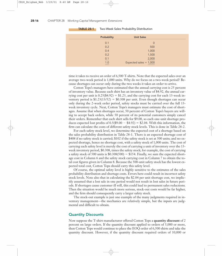
In Chapters 22 and 23, we presented the basic elements of current asset managementand short-term financing. This chapter presents a more in-depth treatment of severalworking capital topics, including (1) the target cash balance, (2) accounting for inven-tory, (3) the EOQ model, and (4) monitoring the receivables position.

Setting the Target Cash Balance

In Chapter 22, when we discussed MicroDrive Inc.’s cash budget, we took as a giventhe $10 million target cash balance. We also discussed how lockboxes, synchronizinginflows and outflows, and float can reduce the required cash balance. Now we considerhow target cash balances are set in practice.

Note (1) that cash per se earns no return, (2) that it is an asset that appears on theleft side of the balance sheet, (3) that cash holdings must be financed by raising eitherdebt or equity, and (4) that both debt and equity capital have a cost. If cash holdingscould be reduced without hurting sales or other aspects of a firm’s operations, this re-duction would permit a reduction in either debt or equity, or both, which would in-crease the return on capital and thus boost the value of the firm’s stock. Therefore, thegeneral operating goal of the cash manager is to minimize the amount of cash held subject tothe constraint that enough cash be held to enable the firm to operate efficiently.

For most firms, cash as a percentage of assets and/or sales has declined sharply inrecent years as a direct result of technological developments in computers andtelecommunications. Years ago, it was difficult to move money from one location toanother, and it was also difficult to forecast exactly how much cash would be needed indifferent locations at different points in time. As a result, firms had to hold relativelylarge “safety stocks” of cash to be sure they had enough when and where it wasneeded. Also, they held relatively large amounts of short-term securities as a backup,and they also had backup lines of credit that permitted them to borrow on short noticeto build up the cash account if it became depleted.

Now think how computers and telecommunications affect the situation. With agood computer system, tied together with good telecommunications links, a companycan get real-time information on its cash balances, whether it operates in a single lo-cation or all over the world. Further, it can use statistical procedures to forecast cashinflows and outflows, and good forecasts reduce the need for safety stocks. Finally, im-provements in telecommunications systems make it possible for a treasurer to replen-ish his or her cash accounts within minutes by simply calling a lender and stating thatthe firm wants to borrow a given amount under its line of credit. The lender thenwires the funds to the desired location. Similarly, marketable securities can be soldwith close to the same speed and with the same minimal transactions costs.

General Telephone (Gen Tel) can be used to illustrate this. Gen Tel knows exactlyhow much it must pay and when, and it can forecast quite accurately when it willreceive checks. For example, the treasurer of Gen Tel’s Florida operation knows whenthe major employers in Tampa pay their workers and how long after that people gen-erally pay their phone bills. Armed with this information, Gen Tel’s Florida treasurercan forecast with great accuracy any cash surpluses or deficits on a daily basis. Ofcourse, no forecast will be exact, so slight overages or underages will occur. But thispresents no problem. The treasurer knows by 11 A.M. the checks that must be coveredby 4 P.M. that day, how much cash has come in, and consequently how much of a cashsurplus or deficit will exist. Then a simple phone call is made, and the company bor-rows to cover any deficit or buys securities (or pays off outstanding loans) with anysurplus. Thus, Gen Tel can maintain cash balances that are very close to zero, a situa-tion that would have been impossible a few years ago.

28-2 CHAPTER 28 Working Capital Management: Extensions

CDThe textbook’s CD-ROMcontains an Excel file thatwill guide you through thechapter’s calculations. Thefile for this chapter is Ch 28Tool Kit.xls, and we encour-age you to open the file andfollow along as you read thechapter.

CH28_Brigham_Web 3/29/01 8:40 AM 8-2

Today, cash management in reasonably sophisticated firms is largely a job for sys-tems people, and, except for the very largest firms, it is generally most efficient to have abank handle the actual operations of the cash management system. Banks do this for aliving, and there are economies of scale in operating cash management systems. Also,many banks are willing and able to offer such services, so competition has driven thecost of cash management down to a reasonable level. Still, it is essential that corporatetreasurers know enough about cash management procedures to be able to negotiate andthen work with the banks to ensure that they get the best price (interest rate) on creditlines, the best yield on short-term investments, and a reasonable cost for other bankingservices. To provide perspective on these issues, we discuss next a theoretical model forcash balances plus a practical approach to setting the target cash balance.

The Baumol Model

William Baumol first noted that cash balances are, in many respects, similar to inven-tories, and that the EOQ inventory model, which will be developed in a later section,can be used to establish a target cash balance.2 Baumol’s model assumes that the firmuses cash at a steady, predictable rate—say, $1,000,000 per week—and that the firm’scash inflows from operations also occur at a steady, predictable rate—say, $900,000per week. Therefore, the firm’s net cash outflows, or net need for cash, also occur at asteady rate—in this case, $100,000 per week.3 Under these steady-state assumptions,the firm’s cash position will resemble the situation shown in Figure 28-1.

Setting the Target Cash Balance 28-3

0 1 2 3 4 5 6 7 8 9 10 11 12

Cash Balances ($)

Weeks

Maximum Cash = C

Average Cash = C/2

Ending Cash = 0

FIGURE 28-1 Cash Balances under the Baumol Model’s Assumptions

2William J. Baumol, “The Transactions Demand for Cash: An Inventory Theoretic Approach,” QuarterlyJournal of Economics, November 1952, 545–556.3Our hypothetical firm is experiencing a $100,000 weekly cash shortfall, but this does not necessarily implythat it is headed for bankruptcy. The firm could, for example, be highly profitable and be enjoying high earn-ings, but be expanding so rapidly that it is experiencing chronic cash shortages that must be made up by bor-rowing or by selling common stock. Or, the firm could be in the construction business and therefore receivemajor cash inflows at wide intervals, but have net cash outflows of $100,000 per week between major inflows.


If our illustrative firm started at Time 0 with a cash balance of C � $300,000, andif its outflows exceeded its inflows by $100,000 per week, then its cash balance woulddrop to zero at the end of Week 3, and its average cash balance would be C/2 �$300,000/2 � $150,000. Therefore, at the end of Week 3 the firm would have to re-plenish its cash balance, either by selling marketable securities, if it had any, or byborrowing.

If C were set at a higher level, say, $600,000, then the cash supply would last longer(six weeks), and the firm would have to sell securities (or borrow) less frequently.However, its average cash balance would rise from $150,000 to $300,000. Brokerageor some other type of transactions cost must be incurred to sell securities (or toborrow), so holding larger cash balances will lower the transactions costs associatedwith obtaining cash. On the other hand, cash provides no income, so the larger the average cash balance, the higher the opportunity cost, which is the return that couldhave been earned on securities or other assets held in lieu of cash. Thus, we have thesituation that is graphed in Figure 28-2. The optimal cash balance is found by usingthe following variables and equations:

C � amount of cash raised by selling marketable securities or by borrowing. C/2 � average cash balance.

C* � optimal amount of cash to be raised by selling marketable securities or byborrowing. C*/2 � optimal average cash balance.

F � fixed costs of selling securities or of obtaining a loan.T � total amount of net new cash needed for transactions during the entire period

(usually a year).k � opportunity cost of holding cash, set equal to either the rate of return fore-

gone on marketable securities or the cost of borrowing to hold cash.


0

Transactions Cost

Total Costs of Holding Cash

C*Optimal

Cash Transfer

Cash Transferred ($)

Costs of Holding Cash ($)

Opportunity Cost

FIGURE 28-2 Determination of the Target Cash Balance


The total costs of cash balances consist of holding (or opportunity) costs plus transac-tions costs:4

(28-1)

The minimum total costs are achieved when C is set equal to C*, the optimal cashtransfer. C* is found as follows:5

(28-2)

Equation 28-2 is the Baumol model for determining optimal cash balances. To illus-trate its use, suppose F � $150; T � 52 weeks � $100,000/week � $5,200,000; and k �15% � 0.15. Then

Therefore, the firm should sell securities (or borrow if it does not hold securities) inthe amount of $101,980 when its cash balance approaches zero, thus building its cashbalance back up to $101,980. If we divide T by C*, we have the number of transactionsper year: $5,200,000/$101,980 � 50.99 � 51, or about once a week. The firm’s aver-age cash balance is $101,980/2 � $50,990 � $51,000.

Note that the optimal cash balance increases less than proportionately with in-creases in the amount of cash needed for transactions. For example, if the firm’s size,and consequently its net new cash needs, doubled from $5,200,000 to $10,400,000 peryear, average cash balances would increase by only 41 percent, from $51,000 to$72,000. This suggests that there are economies of scale in holding cash balances, andthis, in turn, gives larger firms an edge over smaller ones.6

Of course, the firm would probably want to hold a safety stock of cash designed toreduce the probability of a cash shortage. However, if the firm is able to sell securitiesor to borrow on short notice—and most larger firms can do so in a matter of minutessimply by making a telephone call—the safety stock can be quite low.

The Baumol model is obviously simplistic. Most important, it assumes relativelystable, predictable cash inflows and outflows, and it does not take into account sea-sonal or cyclical trends. Other models have been developed to deal both with uncer-tainty and with trends, but all of them have limitations and are more useful as concep-tual models than for actually setting target cash balances.

C* � B2($150)($5,200,000)0.15

� $101,980.

C* � B2(F)(T)k

.

TC

(F).�C2

(k)�

� aAverage cashbalance b aOpportunity

cost rate b � aNumber oftransactionsb a Cost per

transactionbTransactions costs�Holding costsTotal

costs �

Setting the Target Cash Balance 28-5

4Total costs can be expressed on either a before-tax or an after-tax basis. Both methods lead to the same con-clusions regarding target cash balances and comparative costs. For simplicity, we present the model here ona before-tax basis.5Equation 28-1 is differentiated with respect to C. The derivative is set equal to zero, and we then solve forC � C* to derive Equation 28-2. This model, applied to inventories and called the EOQ model, is discussedfurther in a later section.6This edge may, of course, be more than offset by other factors—after all, cash management is only oneaspect of running a business.


Monte Carlo Simulation

Although the Baumol model and other theoretical models provide insights into the op-timal cash balance, they are generally not practical for actual use. Rather, firms gener-ally set their target cash balances based on some “safety stock” of cash that holds the riskof running out of money to some acceptably low level. One commonly used procedureis Monte Carlo simulation.7 To illustrate, consider the cash budget for MicroDrive Inc.presented back in Table 22-1 in Chapter 22. Sales and collections are the driving forcesin the cash budget and, of course, are subject to uncertainty. In the cash budget, we usedexpected values for sales and collections, as well as for all other cash flows. However, itwould be relatively easy to use Monte Carlo simulation, first discussed in Chapter 14, tointroduce uncertainty. If the cash budget were constructed using a spreadsheet programwith Monte Carlo add-in software, then the key uncertain variables could be specifiedas continuous probability distributions rather than point values.

The end result of the simulation would be a distribution for each month’s net cashgain or loss instead of the single values shown on Line 16 of Table 22-1. Suppose Sep-tember’s net cash loss distribution looked like this (in millions):


7See Eugene M. Lerner, “Simulating a Cash Budget,” in Readings on the Management of Working Capital, 2ded., Keith V. Smith, ed. (St. Paul, Minn.: West, 1980).

September Cash Loss Probability of This Loss or More

($83) 10%(75) 20(68) 30(62) 40(57) Expected loss 50(52) 60(46) 70(39) 80(31) 90

Now suppose MicroDrive’s managers want to be 90 percent confident that the firmwill not run out of cash during September, and they do not want to have to borrow tocover any shortfall. They would set the beginning-of-month balance at $83 million,well above the current $10 million, because there is only a 10 percent probability thatSeptember’s cash flow will be worse than an $83 million outflow. With a balance of$83 million at the beginning of the month, there would be only a 10 percent chancethat MicroDrive would run out of cash during September. Of course, Monte Carlosimulation could be applied to the remaining months in the Table 22-1 cash budget,and the amounts obtained to meet some confidence level could be used to set eachmonth’s target cash balance instead of using a fixed target across all months.

The same type of analysis could be used to determine the amount of short-termsecurities to hold, or the size of a requested line of credit. Of course, as in all simula-tions, the hard part is estimating the probability distributions for sales, collections,and the other highly uncertain variables. If these inputs are not good representationsof the actual uncertainty facing the firm, then the resulting target balances will not of-fer the protection against cash shortages implied by the simulation. There is no sub-stitute for experience, and cash managers will adjust the target balances obtained byMonte Carlo simulation on a judgmental basis.


How has technology changed the way target cash balances are set?

What is the Baumol model, and how is it used?

Explain how Monte Carlo simulation can be used to help set a firm’s target cashbalance.

Accounting for Inventory

When finished goods are sold, the firm must assign a cost of goods sold. The cost ofgoods sold appears on the income statement as an expense for the period, and the bal-ance sheet inventory account is reduced by a like amount. Four methods can be usedto value the cost of goods sold, and hence to value the remaining inventory: (1) specificidentification, (2) first-in, first-out (FIFO), (3) last-in, first-out (LIFO), and (4)weighted average.

Specific Identification

Under specific identification, a unique cost is attached to each item in inventory.Then, when an item is sold, the inventory value is reduced by that specific amount.This method is used only when the items are high cost and move relatively slowly,such as cars for an automobile dealer.

First-In, First-Out (FIFO)

In the FIFO method, the units sold during a given period are assumed to be the first units that were placed in inventory. As a result, the cost of goods sold is based on thecost of the oldest inventory items, and the remaining inventory consists of the newestgoods.

Last-In, First-Out (LIFO)

LIFO is the opposite of FIFO. The cost of goods sold is based on the last units placed in inventory, while the remaining inventory consists of the first goods placedin inventory. Note that this is purely an accounting convention—the actual physicalunits sold could be either the earlier or the later units placed in inventory, or somecombination. For example, Del Monte has in its LIFO inventory accounts catsup bottled in the 1920s, but all the catsup in its warehouses was bottled in 2000 or 2001.

Weighted Average

The weighted average method involves calculating the weighted average unit cost ofgoods available for sale from inventory, and this average is then used to determine thecost of goods sold. This method results in a cost of goods sold and an ending inven-tory that fall somewhere between the FIFO and LIFO methods.

Comparison of Inventory Accounting Methods

To illustrate these methods and their effects on financial statements, assume that Cus-tom Furniture Inc. manufactured five identical antique reproduction dining tablesduring a one-year accounting period. During the year, a new labor contract plus

Accounting for Inventory 28-7


dramatically increasing mahogany prices caused manufacturing costs to almost dou-ble, resulting in the following inventory costs:


Cost of Goods Reported Ending InventoryMethod Sales Sold Profit Value

Specific identification $80,000 $42,000 $38,000 $28,000FIFO 80,000 36,000 44,000 34,000LIFO 80,000 48,000 32,000 22,000Weighted average 80,000 42,000 38,000 28,000

There were no tables in stock at the beginning of the year, and Tables 1, 3, and 5 weresold during the year.

If Custom used the specific identification method, the cost of goods sold would bereported as $10,000 � $14,000 � $18,000 � $42,000, while the end-of-period inven-tory value would be $70,000 � $42,000 � $28,000. If Custom used the FIFO method,its cost of goods sold would be $10,000 � $12,000 � $14,000 � $36,000, and endinginventory would be $70,000 � $36,000 � $34,000. If Custom used the LIFO method,its cost of goods sold would be $48,000, and its ending inventory would be $22,000.Finally, if Custom used the weighted average method, its average cost per unit of in-ventory would be $70,000/5 � $14,000, its cost of goods sold would be 3($14,000) �$42,000, and its ending inventory would be $70,000 � $42,000 � $28,000.

If Custom’s actual sales revenues from the tables were $80,000, or an average of$26,667 per unit sold, and if its other costs were minimal, the following is a summaryof the effects of the four methods:

Ignoring taxes, Custom’s cash flows would not be affected by its choice of inven-tory methods, yet its balance sheet and reported profits would vary with each method.In an inflationary period such as in our example, FIFO gives the lowest cost of goodssold and thus the highest net income. FIFO also shows the highest inventory value, soit produces the strongest apparent liquidity position as measured by net working cap-ital or the current ratio. On the other hand, LIFO produces the highest cost of goodssold, the lowest reported profits, and the weakest apparent liquidity position. How-ever, when taxes are considered, LIFO provides the greatest tax deductibility, and thusit results in the lowest tax burden. Consequently, after-tax cash flows are highest ifLIFO is used.

Of course, these results apply only to periods when costs are increasing. If costswere constant, all four methods would produce the same cost of goods sold, ending in-ventory, taxes, and cash flows. However, inflation has been a fact of life in recent years,so most firms use LIFO to take advantage of its greater tax and cash flow benefits.

What are the four methods used to account for inventory?

What effect does the method used have on the firm’s reported profits? On end-ing inventory levels?

Which method should be used if management anticipates a period of inflation?Why?

Table Number: 1 2 3 4 5 TotalCost: $10,000 $12,000 $14,000 $16,000 $18,000 $70,000


The Economic Ordering Quantity (EOQ) Model

As discussed in Chapter 22, inventories are obviously necessary, but it is equally ob-vious that a firm’s profitability will suffer if it has too much or too little inventory.Most firms use a pragmatic approach to setting inventory levels, in which past expe-rience plays a major role. However, as a starting point in the process, it is useful formanagers to consider the insights provided by the economic ordering quantity(EOQ) model. The EOQ model first specifies the costs of ordering and carrying in-ventories and then combines these costs to obtain the total costs associated with in-ventory holdings. Finally, optimization techniques are used to find that order quan-tity, hence inventory level, that minimizes total costs. Note that a third category ofinventory costs, the costs of running short (stock-out costs), are not considered in ourinitial discussion. These costs are dealt with by adding safety stocks, as we will discusslater. Similarly, we shall discuss quantity discounts in a later section. The costs thatremain for consideration at this stage are carrying costs and ordering, shipping, andreceiving costs.

Carrying Costs

Carrying costs generally rise in direct proportion to the average amount of inventorycarried. Inventories carried, in turn, depend on the frequency with which orders areplaced. To illustrate, if a firm sells S units per year, and if it places equal-sized ordersN times per year, then S/N units will be purchased with each order. If the inventory isused evenly over the year, and if no safety stocks are carried, then the average inven-tory, A, will be

(28-3)

For example, if S � 120,000 units in a year, and N � 4, then the firm will order 30,000units at a time, and its average inventory will be 15,000 units:

Just after a shipment arrives, the inventory will be 30,000 units; just before the nextshipment arrives, it will be zero; and on average, 15,000 units will be carried.

Now assume the firm purchases its inventory at a price P � $2 per unit. The aver-age inventory value is thus (P)(A) � $2(15,000) � $30,000. If the firm has a cost ofcapital of 10 percent, it will incur $3,000 in financing charges to carry the inventoryfor one year. Further, assume that each year the firm incurs $2,000 of storage costs(space, utilities, security, taxes, and so forth), that its inventory insurance costs are$500, and that it must mark down inventories by $1,000 because of depreciation andobsolescence. The firm’s total cost of carrying the $30,000 average inventory is thus$3,000 � $2,000 � $500 � $1,000 � $6,500, and the annual percentage cost of carry-ing the inventory is $6,500/$30,000 � 0.217 � 21.7%.

Defining the annual percentage carrying cost as C, we can, in general, find the an-nual total carrying cost, TCC, as the percentage carrying cost, C, times the price perunit, P, times the average number of units, A:

(28-4)

In our example,

TCC � (0.217)($2)(15,000) � $6,500.

TCC � Total carrying cost � (C)(P)(A).

A �S/N

2�

120,000/42

�30,000

2� 15,000 units.

A �Units per order

2�

S/N2

.

The Economic Ordering Quantity (EOQ) Model 28-9


Ordering Costs

Although we assume that carrying costs are entirely variable and rise in direct propor-tion to the average size of inventories, ordering costs are often fixed. For example, thecosts of placing and receiving an order—interoffice memos, long-distance telephonecalls, setting up a production run, and taking delivery—are essentially fixed regardlessof the size of an order, so this part of inventory cost is simply the fixed cost of placingand receiving orders times the number of orders placed per year.8 We define the fixedcosts associated with ordering inventories as F, and if we place N orders per year, thetotal ordering cost is given by Equation 28-5:

(28-5)

Here TOC � total ordering cost, F � fixed costs per order, and N � number of orders placed per year.

Equation 28-3 may be rewritten as N � S/2A, and then substituted into Equation28-5:

(28-6)

To illustrate the use of Equation 28-6, if F � $100, S � 120,000 units, and A � 15,000units, then TOC, the total annual ordering cost, is $400:

Total Inventory Costs

Total carrying cost, TCC, as defined in Equation 28-4, and total ordering cost, TOC,as defined in Equation 28-6, may be combined to find total inventory costs, TIC, asfollows:

(28-7)

Recognizing that the average inventory carried is A � Q/2, or one-half the size ofeach order quantity, Q, we may rewrite Equation 28-7 as follows:

TCC(28-8)

� (C)(P)aQ2b � (F)a S

Qb .

� TOCTIC �

� (C)(P)(A) � F a S2Ab .

� TOCTotal inventory costs � TIC � TCC

TOC � $100a120,00030,000

b � $100(4) � $400.

Total ordering cost � TOC � Fa S2Ab .

Total ordering cost � TOC � (F)(N).


8Note that in reality both carrying and ordering costs can have variable and fixed-cost elements, at least overcertain ranges of average inventory. For example, security and utilities charges are probably fixed in theshort run over a wide range of inventory levels. Similarly, labor costs in receiving inventory could be tied tothe quantity received, and hence could be variable. To simplify matters, we treat all carrying costs as variableand all ordering costs as fixed. However, if these assumptions do not fit the situation at hand, the cost defi-nitions can be changed. For example, one could add another term for shipping costs if there are economiesof scale in shipping, such that the cost of shipping a unit is smaller if shipments are larger. However, in mostsituations shipping costs are not sensitive to order size, so total shipping costs are simply the shipping costper unit times the units ordered (and sold) during the year. Under this condition, shipping costs are not in-fluenced by inventory policy, hence they may be disregarded for purposes of determining the optimal in-ventory level and the optimal order size.


Here we see that total carrying cost equals average inventory in units, Q/2, multipliedby unit price, P, times the percentage annual carrying cost, C. Total ordering costequals the number of orders placed per year, S/Q, multiplied by the fixed cost of plac-ing and receiving an order, F. Finally, total inventory costs equal the sum of total carry-ing cost plus total ordering cost. We will use this equation in the next section to de-velop the optimal inventory ordering quantity.

Derivation of the EOQ Model

Figure 28-3 illustrates the basic premise on which the EOQ model is built, namely,that some costs rise with larger inventories while other costs decline, and there is anoptimal order size (and associated average inventory) that minimizes the total costs ofinventories. First, as noted earlier, the average investment in inventories depends onhow frequently orders are placed and the size of each order—if we order every day, av-erage inventories will be much smaller than if we order once a year. Further, as Figure28-3 shows, the firm’s carrying costs rise with larger orders: larger orders mean largeraverage inventories, so warehousing costs, interest on funds tied up in inventory, in-surance, and obsolescence costs will all increase. However, ordering costs decline withlarger orders and inventories: the cost of placing orders, suppliers’ production set-upcosts, and order handling costs will all decline if we order infrequently and conse-quently hold larger quantities.

If the carrying and ordering cost curves in Figure 28-3 are added, the sum repre-sents total inventory costs, TIC. The point where the TIC is minimized representsthe economic ordering quantity (EOQ), and this, in turn, determines the optimal av-erage inventory level.

The EOQ is found by differentiating Equation 28-8 with respect to orderingquantity, Q, and setting the derivative equal to zero:

d(TIC)dQ

�(C)(P)

2�

(F)(S)Q2 � 0.


FIGURE 28-3 Determination of the Optimal Order Quantity

Costs of Ordering andCarrying Inventories ($)

0 EOQ Order Size (Units)

Total Inventory Costs (TIC)

Total Carrying Cost (TCC)

Total Ordering Cost (TOC)


Now, solving for Q we obtain:

(28-9)

Here

EOQ � economic ordering quantity, or the optimal quantity to be ordered eachtime an order is placed.

F � fixed costs of placing and receiving an order.S � annual sales in units.C � annual carrying costs expressed as a percentage of average inventory

value.P � purchase price the firm must pay per unit of inventory.

Equation 28-9 is the EOQ model.9 The assumptions of the model, which will berelaxed shortly, include the following: (1) sales can be forecasted perfectly, (2) sales areevenly distributed throughout the year, and (3) orders are received when expected.

EOQ Model Illustration

To illustrate the EOQ model, consider the following data supplied by Cotton TopsInc., a distributor of budget-priced, custom-designed T-shirts that it sells to conces-sionaires at various theme parks in the United States:

S � annual sales � 26,000 shirts per year.C � percentage carrying cost � 25 percent of inventory value.P � purchase price per shirt � $4.92 per shirt. (The sales price is $9, but this is ir-

relevant for our purposes here.)F � fixed cost per order � $1,000. Cotton Tops designs and distributes the shirts,

but the actual production is done by another company. The bulk of this $1,000cost is the labor cost for setting up the equipment for the production run,which the manufacturer bills separately from the $4.92 cost per shirt.

Substituting these data into Equation 28-9, we obtain an EOQ of 6,500 units:

� 242,276,423 � 6,500 units.

EOQ � B2(F)(S)(C)(P)

� B (2)($1,000)(26,000)(0.25)($4.92)

Q � EOQ � B2(F)(S)(C)(P)

.

Q2 �2(F)(S)(C)(P)

(C)(P)2

�(F)(S)

Q2


9The EOQ model can also be written as

where C* is the annual carrying cost per unit expressed in dollars.

EOQ � B2(F)(S)C*

,


With an EOQ of 6,500 shirts and annual usage of 26,000 shirts, Cotton Tops willplace 26,000/6,500 � 4 orders per year. Note that average inventory holdings dependdirectly on the EOQ. This relationship is illustrated graphically in Figure 28-4, wherewe see that average inventory � EOQ/2. Immediately after an order is received, 6,500shirts are in stock. The usage rate, or sales rate, is 500 shirts per week (26,000/52weeks), so inventories are drawn down by this amount each week. Thus, the actualnumber of units held in inventory will vary from 6,500 shirts just after an order is re-ceived to zero just before a new order arrives. With a 6,500 beginning balance, a zeroending balance, and a uniform sales rate, inventories will average one-half the EOQ,or 3,250 shirts, during the year. At a cost of $4.92 per shirt, the average investment ininventories will be (3,250)($4.92) � $16,000. If inventories are financed by bank loans,the loan will vary from a high of $32,000 to a low of $0, but the average amount out-standing over the course of a year will be $16,000.

Note that the EOQ, hence average inventory holdings, rises with the square rootof sales. Therefore, a given increase in sales will result in a less-than-proportionate in-crease in inventories, so the inventory/sales ratio will tend to decline as a firm grows.For example, Cotton Tops’s EOQ is 6,500 shirts at an annual sales level of 26,000, andthe average inventory is 3,250 shirts, or $16,000. However, if sales were to increase by100 percent, to 52,000 shirts per year, the EOQ would rise only to 9,195 units, or by41 percent, and the average inventory would rise by this same percentage. This sug-gests that there are economies of scale in holding inventories.10


10Note, however, that these scale economies relate to each particular item, not to the entire firm. Thus, alarge distributor with $500 million of sales might have a higher inventory/sales ratio than a much smallerdistributor if the small firm has only a few high-sales-volume items while the large firm distributes a greatmany low-volume items.

FIGURE 28-4 Inventory Position without Safety Stock

2 4 6 8 10 12 14 16 18 20 22 24 26 280

1

2

3

4

5

6

7

8

6.5

Order Lead Time = 2 Weeks or 14 Days

EOQ

Units(in Thousands)

Maximum Inventory= 6,500 = EOQ

Slope = Sales Rate = 500 Shirts per Week

AverageInventory= 3,250

Order Point= 1,000

Weeks


Finally, look at Cotton Tops’s total inventory costs for the year, assuming that theEOQ is ordered each time. Using Equation 28-8, we find total inventory costs are$8,000:

Note these two points: (1) The $8,000 total inventory cost represents the total of car-rying costs and ordering costs, but this amount does not include the 26,000($4.92) �$127,920 annual purchasing cost of the inventory itself. (2) As we see both in Figure28-3 and in the calculation above, at the EOQ, total carrying cost (TCC) equals totalordering cost (TOC). This property is not unique to our Cotton Tops illustration; italways holds.

Setting the Order Point

If a two-week lead time is required for production and shipping, what is Cotton Tops’sorder point level? Cotton Tops sells 26,000/52 � 500 shirts per week. Thus, if a two-week lag occurs between placing an order and receiving goods, Cotton Tops mustplace the order when there are 2(500) � 1,000 shirts on hand. During the two-weekproduction and shipping period, the inventory balance will continue to decline at therate of 500 shirts per week, and the inventory balance will hit zero just as the order ofnew shirts arrives.

If Cotton Tops knew for certain that both the sales rate and the order lead timewould never vary, it could operate exactly as shown in Figure 28-4. However, sales dochange, and production and/or shipping delays are sometimes encountered. To guardagainst these events, the firm must carry additional inventories, or safety stocks, as dis-cussed in the next section.

What are some specific inventory carrying costs? As defined here, are thesecosts fixed or variable?

What are some inventory ordering costs? As defined here, are these costs fixedor variable?

What are the components of total inventory costs?

What is the concept behind the EOQ model?

What is the relationship between total carrying cost and total ordering cost atthe EOQ?

What assumptions are inherent in the EOQ model as presented here?

EOQ Model Extensions

The basic EOQ model was derived under several restrictive assumptions. In this sec-tion, we relax some of these assumptions and, in the process, extend the model tomake it more useful.

The Concept of Safety Stocks

The concept of a safety stock is illustrated in Figure 28-5. First, note that the slope ofthe sales line measures the expected rate of sales. The company expects to sell 500

� $8,000.$4,000�$4,000�

� 0.25($4.92)a6,5002b � ($1,000)a26,000

6,500b

(F) a SQb�(C)(P)aQ

2b�

TOC�TCCTIC �



shirts per week, but let us assume that the maximum likely sales rate is twice thisamount, or 1,000 units each week. Further, assume that Cotton Tops sets the safetystock at 1,000 shirts, so it initially orders 7,500 shirts, the EOQ of 6,500 plus the1,000-unit safety stock. Subsequently, it reorders the EOQ whenever the inventorylevel falls to 2,000 shirts, the safety stock of 1,000 shirts plus the 1,000 shirts expectedto be used while awaiting delivery of the order.

Note that the company could, over the two-week delivery period, sell 1,000 unitsa week, or double its normal expected sales. This maximum rate of sales is shown bythe steeper dashed line in Figure 28-5. The condition that makes this higher sales ratepossible is the safety stock of 1,000 shirts.

The safety stock is also useful to guard against delays in receiving orders. The ex-pected delivery time is two weeks, but with a 1,000-unit safety stock, the companycould maintain sales at the expected rate of 500 units per week for an additional twoweeks if something should delay an order.

However, carrying a safety stock has a cost. The average inventory is now EOQ/2plus the safety stock, or 6,500/2 � 1,000 � 3,250 � 1,000 � 4,250 shirts, and the av-erage inventory value is now (4,250)($4.92) � $20,910. This increase in average in-ventory causes an increase in annual inventory carrying costs equal to (Safetystock)(P)(C) � 1,000($4.92)(0.25) � $1,230.

The optimal safety stock varies from situation to situation, but, in general, it in-creases (1) with the uncertainty of demand forecasts, (2) with the costs (in terms of lostsales and lost goodwill) that result from inventory shortages, and (3) with the proba-bility that delays will occur in receiving shipments. The optimal safety stock decreasesas the cost of carrying this additional inventory increases.

Setting the Safety Stock Level

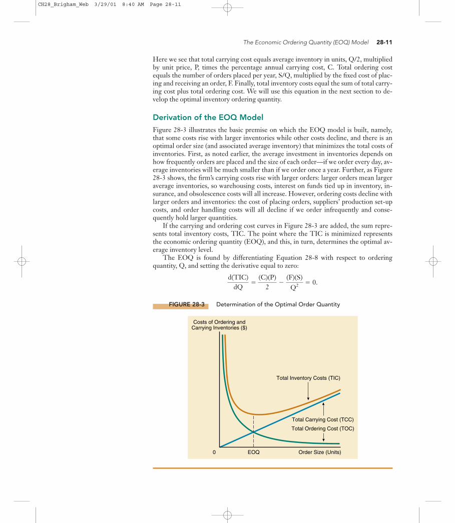
The critical question with regard to safety stocks is this: How large should the safetystock be? To answer this question, first examine Table 28-1, which contains the prob-ability distribution of Cotton Tops’s unit sales for an average two-week period, the

EOQ Model Extensions 28-15

FIGURE 28-5 Inventory Position with Safety Stock Included

2 4 6 8 10 12 14 16 18 20 22 24 26 280

1

2

3

4

5

6

7

8

Lead Time

EOQ

Units(in Thousands)

Maximum Sales Rate

30Weeks

AverageSales Rate

MaximumInventory

SafetyStock

OrderPoint


time it takes to receive an order of 6,500 T-shirts. Note that the expected sales over anaverage two-week period is 1,000 units. Why do we focus on a two-week period? Be-cause shortages can occur only during the two weeks it takes an order to arrive.

Cotton Tops’s managers have estimated that the annual carrying cost is 25 percentof inventory value. Because each shirt has an inventory value of $4.92, the annual car-rying cost per unit is 0.25($4.92) � $1.23, and the carrying cost for each 13-week in-ventory period is $1.23(13/52) � $0.308 per unit. Even though shortages can occuronly during the 2-week order period, safety stocks must be carried over the full 13-week inventory cycle. Next, Cotton Tops’s managers must estimate the cost of short-ages. Assume that when shortages occur, 50 percent of Cotton Tops’s buyers are will-ing to accept back orders, while 50 percent of its potential customers simply canceltheir orders. Remember that each shirt sells for $9.00, so each one-unit shortage pro-duces expected lost profits of 0.5($9.00 � $4.92) � $2.04. With this information, thefirm can calculate the costs of different safety stock levels. This is done in Table 28-2.

For each safety stock level, we determine the expected cost of a shortage based onthe sales probability distribution in Table 28-1. There is an expected shortage cost of$408 if no safety stock is carried; $102 if the safety stock is set at 500 units; and no ex-pected shortage, hence no shortage cost, with a safety stock of 1,000 units. The cost ofcarrying each safety level is merely the cost of carrying a unit of inventory over the 13-week inventory period, $0.308, times the safety stock; for example, the cost of carryinga safety stock of 500 units is $0.308(500) � $154. Finally, we sum the expected short-age cost in Column 6 and the safety stock carrying cost in Column 7 to obtain the to-tal cost figures given in Column 8. Because the 500-unit safety stock has the lowest ex-pected total cost, Cotton Tops should carry this safety level.

Of course, the optimal safety level is highly sensitive to the estimates of the salesprobability distribution and shortage costs. Errors here could result in incorrect safetystock levels. Note also that in calculating the $2.04 per unit shortage cost, we implic-itly assumed that a lost sale in one period would not result in lost sales in future peri-ods. If shortages cause customer ill will, this could lead to permanent sales reductions.Then the situation would be much more serious, stock-out costs would be far higher,and the firm should consequently carry a larger safety stock.

The stock-out example is just one example of the many judgments required in in-ventory management—the mechanics are relatively simple, but the inputs are judg-mental and difficult to obtain.

Quantity Discounts

Now suppose the T-shirt manufacturer offered Cotton Tops a quantity discount of 2percent on large orders. If the quantity discount applied to orders of 5,000 or more,then Cotton Tops would continue to place the EOQ order of 6,500 shirts and take thequantity discount. However, if the quantity discount required orders of 10,000 or


TABLE 28-1 Two-Week Sales Probability Distribution

Probability Unit Sales

0.1 00.2 5000.4 1,0000.2 1,5000.1 2,0001.0 Expected sales � 1,000


EOQ Model Extensions 28-17

more, then Cotton Tops would have to compare the savings in purchase price thatwould result if its ordering quantity were increased to 10,000 units with the increase intotal inventory costs caused by the departure from the 6,500-unit EOQ.

First, consider the total costs associated with Cotton Tops’s EOQ of 6,500 units.We found earlier that total inventory costs are $8,000:

Now, what would total inventory costs be if Cotton Tops ordered 10,000 units insteadof 6,500? The answer is $8,625:

Note that when the discount is taken, the price, P, is reduced by the amount of thediscount; the new price per unit would be 0.98($4.92) � $4.82. Also note that when

� $8,625.$2,600�$6,025�

TIC � 0.25($4.82)a10,0002b � ($1,000)a26,000

10,000b

� $8,000.$4,000�$4,000�

� 0.25($4.92)a6,5002b � ($1,000)a26,000

6,500b

(F)a SQb�(C)(P)aQ

2b�

TOC�TCCTIC �

TABLE 28-2 Safety Stock Analysis

SafetySales During Expected Stock ExpectedTwo-Week Shortage Cost Shortage Carrying Total

Safety Delivery (Lost Profits): Cost: Cost: Cost:Stock Period Probability Shortagea $2.04 � (4) (3) � (5) $0.308 � (1) (6) � (7)

(1) (2) (3) (4) � (5) � (6) � (7) � (8)

0 0 0.1 0 $ 0 $ 0500 0.2 0 0 0

1,000 0.4 0 0 01,500 0.2 500 1,020 2042,000 0.1 1,000 2,040 204

1.0 Expected shortage cost � $408 $ 0 $408

500 0 0.1 0 $ 0 $ 0500 0.2 0 0 0

1,000 0.4 0 0 01,500 0.2 0 0 02,000 0.1 500 1,020 102

1.0 Expected shortage cost � $102 $154 $256

1,000 0 0.1 0 $ 0 $ 0500 0.2 0 0 0

1,000 0.4 0 0 01,500 0.2 0 0 02,000 0.1 0 0 0

1.0 Expected shortage cost � $ 0 $308 $308

aShortage � Actual sales � (1,000 Stock at order point � Safety stock); positive values only.


the ordering quantity is increased, carrying costs increase because the firm is carryinga larger average inventory, but ordering costs decrease since the number of orders peryear decreases. If we were to calculate total inventory costs at an ordering quantityless than the EOQ, say, 5,000, we would find that carrying costs would be less than$4,000, and ordering costs would be more than $4,000, but the total inventory costswould be more than $8,000, since they are at a minimum when 6,500 units are or-dered.11

Thus, inventory costs would increase by $8,625 � $8,000 � $625 if Cotton Topswere to increase its order size to 10,000 shirts. However, this cost increase must be com-pared with Cotton Tops’s savings if it takes the discount. Taking the discount would save0.02($4.92) � $0.0984 per unit. Over the year, Cotton Tops orders 26,000 shirts, sothe annual savings is $0.0984(26,000) � $2,558. Here is a summary:


11At an ordering quantity of 5,000 units, total inventory costs are $8,275:

� $3,075 � $5,200 � $8,275.

TIC � (0.25)($4.92)a5,0002b � ($1,000)a26,000

5,000b

Reduction in purchase price � 0.02($4.92)(26,000) � $2,558Increase in total inventory cost � 625Net savings from taking discounts $1,933

Obviously, the company should order 10,000 units at a time and take advantage of thequantity discount.

Inflation

Moderate inflation—say, 3 percent per year—can largely be ignored for purposes ofinventory management, but higher rates of inflation must be explicitly considered. Ifthe rate of inflation in the types of goods the firm stocks tends to be relatively con-stant, it can be dealt with quite easily—simply deduct the expected annual rate of in-flation from the carrying cost percentage, C, in Equation 28-9, and use this modifiedversion of the EOQ model to establish the ordering quantity. The reason for makingthis deduction is that inflation causes the value of the inventory to rise, thus offsettingsomewhat the effects of depreciation and other carrying costs. C will now be smaller,assuming other factors are held constant, so the calculated EOQ and the average in-ventory will increase. However, higher rates of inflation usually mean higher interestrates, and this will cause C to increase, thus lowering the EOQ and average inventory.

On balance, there is no evidence that inflation either raises or lowers the optimalinventories of firms in the aggregate. Inflation should still be explicitly considered,however, for it will raise the individual firm’s optimal holdings if the rate of inflationfor its own inventories is above average (and is greater than the effects of inflation oninterest rates), and vice versa.

Seasonal Demand

For most firms, it is unrealistic to assume that the demand for an inventory item isuniform throughout the year. What happens when there is seasonal demand, as wouldhold true for an ice cream company? Here the standard annual EOQ model is obvi-ously not appropriate. However, it does provide a point of departure for setting inven-tory parameters, which are then modified to fit the particular seasonal pattern. We


divide the year into the seasons in which annualized sales are relatively constant, say,summer, spring and fall, and winter. Then, the EOQ model is applied separately toeach period. During the transitions between seasons, inventories would be either rundown or else built up with special seasonal orders.

EOQ Range

Thus far, we have interpreted the EOQ and the resulting inventory values as singlepoint estimates. It can be easily demonstrated that small deviations from the EOQ donot appreciably affect total inventory costs, and, consequently, that the optimal order-ing quantity should be viewed more as a range than as a single value.12

To illustrate this point, we examine the sensitivity of total inventory costs to or-dering quantity for Cotton Tops. Table 28-3 contains the results. We conclude thatthe ordering quantity could range from 5,000 to 8,000 units without affecting total in-ventory costs by more than 3.4 percent. Thus, managers can adjust the ordering quan-tity within a fairly wide range without significantly increasing total inventory costs.

Why are safety stocks required?

Conceptually, how would you evaluate a quantity discount offer from a supplier?

What effect does inflation typically have on the EOQ?

Can the EOQ model be used when a company faces seasonal demand fluctua-tions?

What is the effect of minor deviations from the EOQ on total inventory costs?

The Payments Pattern Approach to Monitoring Receivables

In Chapter 22, we discussed two methods for monitoring a firm’s receivables position:days sales outstanding and aging schedules. These procedures are useful, especially formonitoring an individual customer’s account, but neither is totally suitable for moni-toring the aggregate payment performance of all credit customers, especially for afirm that experiences fluctuating credit sales. In this section, we present another wayto monitor receivables, the payments pattern approach.

The Payments Pattern Approach to Monitoring Receivables 28-19

12This is somewhat analogous to the optimal capital structure in that small changes in capital structurearound the optimum do not have much effect on the firm’s weighted average cost of capital.

TABLE 28-3 EOQ Sensitivity Analysis

PercentageOrdering Total Inventory DeviationQuantity Costs from Optimal

3,000 $10,512 �31.4%4,000 8,960 �12.05,000 8,275 �3.46,000 8,023 �0.36,500 8,000 0.07,000 8,019 �0.28,000 8,170 �2.19,000 8,423 �5.3

10,000 8,750 �9.4


The primary point in analyzing the aggregate accounts receivable situation is tosee if customers, on average, are paying more slowly. If so, accounts receivable willbuild up, as will the cost of carrying receivables. Further, the payment slowdown maysignal a decrease in the quality of the receivables, hence an increase in bad debt lossesdown the road. The DSO and aging schedules are useful in monitoring credit opera-tions, but both are affected by increases and decreases in the level of sales. Thus,changes in sales levels, including normal seasonal or cyclical changes, can change afirm’s DSO and aging schedule even though its customers’ payment behavior has notchanged at all. For this reason, a procedure called the payments pattern approach hasbeen developed to measure any changes that might be occurring in customers’ pay-ment behavior.13 To illustrate the payments pattern approach, consider the HanoverCompany, a small manufacturer of hand tools that commenced operations in January2001. Table 28-4 contains Hanover’s credit sales and receivables data for 2001. Col-umn 2 shows that Hanover’s credit sales are seasonal, with the lowest sales in the falland winter months and the highest during the summer.

Now assume that 10 percent of Hanover’s customers pay in the month the sale ismade, that 30 percent pay in the first month following the sale, that 40 percent payin the second month, and that the remaining 20 percent pay in the third month. Fur-ther, assume that Hanover’s customers have the same payment behavior through-out the year; that is, they always take the same length of time to pay. Column 3 ofTable 28-4 contains Hanover’s receivables balance at the end of each month. For ex-ample, during January Hanover had $60,000 in sales. Ten percent of the customerspaid during the month of sale, so the receivables balance at the end of January was


TABLE 28-4 Hanover Company: Receivables Data for 2001 (Thousands of Dollars)

Based on Based onQuarterly Year-to-Date

Receivables Sales Data Sales DataCredit Sales at End of

Month for Month Month ADSa DSOb ADS DSO(1) (2) (3) (4) (5) (6) (7)

January $ 60 $ 54February 60 90March 60 102 $2.00 51 days $2.00 51 days

April 60 102May 90 129June 120 174 3.00 58 2.50 70

July 120 198August 90 177September 60 132 3.00 44 2.67 49

October 60 108November 60 102December 60 102 2.00 51 2.50 41

aADS � Average daily sales.bDSO � Days sales outstanding.

13See Wilbur G. Lewellen and Robert W. Johnson, “A Better Way to Monitor Accounts Receivable,” Har-vard Business Review, May–June 1972, 101–109; and Bernell Stone, “The Payments-Pattern Approach to theForecasting and Control of Accounts Receivable,” Financial Management, Autumn 1976, 65–82.


$60,000 � 0.1($60,000) � (1.0 � 0.1)($60,000) � 0.9($60,000) � $54,000. By theend of February, 10% � 30% � 40% of the customers had paid for January’s sales,and 10 percent had paid for February’s sales. Thus, the receivables balance at the endof February was 0.6($60,000) � 0.9($60,000) � $90,000. By the end of March, 80percent of January’s sales had been collected, 40 percent of February’s had been col-lected, and 10 percent of March’s sales had been collected, so the receivables balancewas 0.2($60,000) � 0.6($60,000) � 0.9($60,000) � $102,000; and so on.

Columns 4 and 5 give Hanover’s average daily sales (ADS) and days sales outstand-ing (DSO), respectively, as these measures would be calculated from quarterly finan-cial statements. For example, in the April–June quarter, ADS � ($60,000 � $90,000 �$120,000)/90 � $3,000, and the end-of-quarter (June 30) DSO � $174,000/$3,000 �58 days. Columns 6 and 7 also show ADS and DSO, but here they are calculated onthe basis of accumulated sales throughout the year. For example, at the end of JuneADS � $450,000/180 � $2,500 and DSO � $174,000/$2,500 � 70 days. (For the en-tire year, sales are $900,000; ADS � $2,500, and DSO at year-end � 41 days. Theselast two figures are shown at the bottom of the last two columns.)

The data in Table 28-4 illustrate two major points. First, fluctuating sales lead tochanges in the DSO, which suggests that customers are paying faster or slower, eventhough we know that customers’ payment patterns are not changing at all. The risingmonthly sales trend causes the calculated DSO to rise, whereas falling sales (as in thethird quarter) cause the calculated DSO to fall, even though nothing is changing withregard to when customers actually pay. Second, we see that the DSO depends on anaveraging procedure, but regardless of whether quarterly, semiannual, or annual dataare used, the DSO is still unstable even though payment patterns are not changing.Therefore, it is difficult to use the DSO as a monitoring device if the firm’s sales ex-hibit seasonal or cyclical patterns.

Seasonal or cyclical variations also make it difficult to interpret aging schedules.Table 28-5 contains Hanover’s aging schedules at the end of each quarter of 2001. Atthe end of June, Table 28-4 showed that Hanover’s receivables balance was $174,000.Eighty percent of April’s $60,000 of sales had been collected, 40 percent of May’s$90,000 of sales had been collected, and 10 percent of June’s $120,000 of sales hadbeen collected. Thus, the end-of-June receivables balance consisted of 0.2($60,000) �$12,000 of April sales, 0.6($90,000) � $54,000 of May sales, and 0.9($120,000) �$108,000 of June sales. Note again that Hanover’s customers had not changed theirpayment patterns. However, rising sales during the second quarter created the im-pression of faster payments when judged by the percentage aging schedule, and fallingsales after July created the opposite appearance. Thus, neither the DSO nor the agingschedule provides an accurate picture of customers’ payment patterns if sales fluctuateduring the year or are trending up or down.

The Payments Pattern Approach to Monitoring Receivables 28-21

TABLE 28-5 Hanover Company: Quarterly Aging Schedules for 2001 (Thousands of Dollars)

Value and Percentage of Total Accounts ReceivableAge of at the End of Each Quarter:

Accounts(Days) March 31 June 30 September 30 December 31

0–30 $ 54 53% $108 62% $ 54 41% $ 54 53%31–60 36 35 54 31 54 41 36 3561–90 12 12 12 7 24 18 12 12

$102 100% $174 100% $132 100% $102 100%


With this background, we can now examine another basic tool, the uncollected bal-ances schedule, as shown in Table 28-6. At the end of each quarter, the dollar amount ofreceivables remaining from each of the three month’s sales is divided by that month’ssales to obtain three receivables-to-sales ratios. For example, at the end of the first quar-ter $12,000 of the $60,000 January sales, or 20 percent, are still outstanding; 60 percentof February sales are still out; and 90 percent of March sales are uncollected. Exactly thesame situation is revealed at the end of each of the next three quarters. Thus, Table 28-6shows that Hanover’s customers’ payment behavior has remained constant.

Recall that at the beginning of the example we assumed the existence of a constantpayments pattern. In a normal situation, the firm’s customers’ payments pattern wouldprobably vary somewhat over time. Such variations would be shown in the last columnof the uncollected balances schedule. For example, suppose customers began to paytheir accounts slower in the second quarter. That might cause the second quarter un-collected balances schedule to look like this (in thousands of dollars):


TABLE 28-6 Hanover Company: Quarterly Uncollected Balances Schedules for 2001 (Thousands of Dollars)

Remaining Receivablesas Percent of

Remaining Receivables Month’s Sales atQuarter Monthly Sales at End of Quarter End of Quarter

Quarter 1:January $ 60 $ 12 20%February 60 36 60March 60 54 90

$102 170%

Quarter 2:April $ 60 $ 12 20%May 90 54 60June 120 108 90

$174 170%

Quarter 3:July $120 $ 24 20%August 90 54 60September 60 54 90

$132 170%

Quarter 4:October $ 60 $ 12 20%November 60 36 60December 60 54 90

$102 170%

Quarter 2, New Remaining New2001 Sales Receivables Receivables/Sales

April $ 60 $ 16 27%May 90 70 78June 120 110 92

$196 197%


Analyzing Proposed Changes in Credit Policy 28-23

We see that the receivables-to-sales ratios are now higher than in the correspondingmonths of the first quarter. This causes the total uncollected balances percentage torise from 170 to 197 percent, which, in turn, should alert Hanover’s managers thatcustomers are paying slower than they did earlier in the year.

The uncollected balances schedule permits a firm to monitor its receivables better,and it can also be used to forecast future receivables balances. When Hanover’s proforma 2002 quarterly balance sheets are constructed, management can use the histor-ical receivables-to-sales ratios, coupled with 2002 sales estimates, to project each quar-ter’s receivables balance. For example, with projected sales as given below, and usingthe same payments pattern as in 2001, Hanover’s projected end-of-June 2002 receiv-ables balance would be as follows:

The payments pattern approach permits us to remove the effects of seasonaland/or cyclical sales variation and to construct a more accurate measure of customers’payments patterns. Thus, it provides financial managers with better aggregate infor-mation than the days sales outstanding or the aging schedule. Managers should use thepayments pattern approach to monitor collection performance as well as to projectfuture receivables requirements.

Except possibly in the inventory and cash management areas, nowhere in the typ-ical firm have computers had more of an effect than in accounts receivable manage-ment. A well-run business will use a computer system to record sales, to send out bills,to keep track of when payments are made, to alert the credit manager when an accountbecomes past due, and to take action automatically to collect past-due accounts (forexample, to prepare form letters requesting payment). Additionally, the payment his-tory of each customer can be summarized and used to help establish credit limits forcustomers and classes of customers, and the data on each account can be aggregatedand used for the firm’s accounts receivable monitoring system. Finally, historical datacan be stored in the firm’s database and used to develop inputs for studies related tocredit policy changes, as we discuss in the next section.

Define days sales outstanding (DSO). What can be learned from it? Does it haveany deficiencies when used to monitor collections over time?

What is an aging schedule? What can be learned from it? Does it have any defi-ciencies when used to monitor collections over time?

What is the uncollected balances schedule? What advantages does it have overthe DSO and the aging schedule for monitoring receivables? How can it be usedto forecast a firm’s receivables balance?

Analyzing Proposed Changes in Credit Policy

In Chapter 22, we discussed credit policy, including setting the credit period, creditstandards, collection policy, and discount percentage, as well as the factors thatinfluence credit policy. A firm’s credit policy is reviewed periodically, and policy

Quarter 2, 2002 Projected Sales Receivables/Sales Projected Receivables

April $ 70,000 20% $ 14,000May 100,000 60 60,000June 140,000 90 126,000

Total projected receivables � $200,000


changes may be proposed. However, before a new policy is adopted, it should be ana-lyzed to determine if it is indeed preferable to the existing policy. In this section, wediscuss procedures for analyzing proposed changes in credit policy.

If a firm’s credit policy is eased by such actions as lengthening the credit period, re-laxing credit standards, following a less tough collection policy, or offering cash dis-counts, then sales should increase: Easing the credit policy stimulates sales. Of course, ifcredit policy is eased and sales rise, then costs will also rise because more labor, mate-rials, and so on, will be required to produce the additional goods. Additionally, receiv-ables outstanding will also increase, which will increase carrying costs. Moreover, baddebts and/or discount expenses may also rise. Thus, the key question when decidingon a proposed credit policy change is this: Will sales revenues increase more thancosts, including credit-related costs, causing cash flow to increase, or will the increasein sales revenues be more than offset by higher costs?

Table 28-7 illustrates the general idea behind the analysis of credit policy changes.Column 1 shows the projected 2002 income statement for Monroe Manufacturing un-der the assumption that the firm’s current credit policy is maintained throughout theyear. Column 2 shows the expected effects of easing the credit policy by extending thecredit period, offering larger discounts, relaxing credit standards, and easing collectionefforts. Specifically, Monroe is analyzing the effects of changing its credit terms from1/10, net 30, to 2/10, net 40, relaxing its credit standards, and putting less pressure onslow-paying customers. Column 3 shows the projected 2002 income statement incor-porating the expected effects of an easing in credit policy. The generally looser policy isexpected to increase sales and lower collection costs, but discounts and several othertypes of costs would rise. The overall, bottom-line effect is a $7 million increase inprojected net income. In the following paragraphs, we explain how the numbers in thetable were calculated.

Monroe’s annual sales are $400 million. Under its current credit policy, 50 per-cent of those customers who pay do so on Day 10 and take the discount, 40 percentpay on Day 30, and 10 percent pay late, on Day 40. Thus, Monroe’s days sales


TABLE 28-7 Monroe Manufacturing Company: Analysis of Changing Credit Policy (Millions of Dollars)

Projected 2002 Projected 2002Net Income Effect of Net Income

Under Current Credit Policy Under NewCredit Policy Change Credit Policy

(1) (2) (3)

Gross sales $400 �$130 $530Less discounts 2 � 4 6

Net sales $398 �$126 $524Production costs, including overhead 280 � 91 371

Profit before credit costs and taxes $118 �$ 35 $153Credit-related costs:

Cost of carrying receivables 3 � 2 5Credit analysis and collection expenses 5 � 3 2Bad debt losses 10 � 22 32

Profit before taxes $100 �$ 14 $114State-plus-federal taxes (50%) 50 � 7 57Net income $ 50 �$ 7 $ 57

Note: The above statements include only those cash flows incremental to the credit policy decision.


outstanding is (0.5)(10) � (0.4)(30) � (0.1)(40) � 21 days, and discounts total(0.01)($400,000,000)(0.5) � $2,000,000.

The cost of carrying receivables is equal to the average receivables balance timesthe variable cost percentage times the cost of money used to carry receivables. Thefirm’s variable cost ratio is 70 percent, and its pre-tax cost of capital invested in receiv-ables is 20 percent. Thus, its annual cost of carrying receivables is $3 million:

Only variable costs enter this calculation because this is the only cost element in re-ceivables that must be financed. We are seeking the cost of carrying receivables, andvariable costs represent the firm’s investment in the cost of goods sold.

Even though Monroe spends $5 million annually to analyze accounts and to col-lect bad debts, 2.5 percent of sales will never be collected. Bad debt losses thereforeamount to (0.025)($400,000,000) � $10,000,000.

Monroe’s new credit policy would be 2/10, net 40 versus the old policy of 1/10, net30, so it would call for a larger discount and a longer payment period, as well as a re-laxed collection effort and lower credit standards. The company believes that thesechanges will lead to a $130 million increase in sales, to $530 million per year. Underthe new terms, management believes that 60 percent of the customers who pay willtake the 2 percent discount, so discounts will increase to (0.02)($530,000,000)(0.60) �$6,360,000 � $6 million. Half of the nondiscount customers will pay on Day 40, andthe remainder on Day 50. The new DSO is thus estimated to be 28 days:

Also, the cost of carrying receivables will increase to $5 million:

The company plans to reduce its annual credit analysis and collection expenditures to$2 million. The reduced credit standards and the relaxed collection effort are expectedto raise bad debt losses to about 6 percent of sales, or to (0.06)($530,000,000) �$31,800,000 � $32,000,000, which is an increase of $22 million from the previouslevel.

The combined effect of all the changes in credit policy is a projected $7 millionannual increase in net income. There would, of course, be corresponding changes onthe projected balance sheet—the higher sales would necessitate somewhat larger cashbalances, inventories, and, depending on the capacity situation, perhaps more fixedassets. Accounts receivable would, of course, also increase. Because these asset in-creases would have to be financed, certain liabilities and/or equity would have to beincreased.

(24)($530,000,000/360)(0.70)(0.20) � $4,946,667 � $5 million.14

(0.6)(10) � (0.2)(40) � (0.2)(50) � 24 days.

(21)($400,000,000/360)(0.70)(0.20) � $3,266,667 � $3 million.

(DSO)°Salesperday¢ °Variable

costratio

¢ ° Costof

funds¢ � Cost of carrying receivables

Analyzing Proposed Changes in Credit Policy 28-25

14Since the credit policy change will result in a longer DSO, the firm will have to wait longer to receive itsprofit on the goods it sells. Therefore, the firm will incur an opportunity cost due to not having the cashfrom these profits available for investment. The dollar amount of this opportunity cost is equal to the oldsales per day times the change in DSO times the contribution margin (1 � Variable cost ratio) times thefirm’s cost of carrying receivables, or

For simplicity, we have ignored this opportunity cost in our analysis. However, we consider opportunitycosts in the next section, where we discuss incremental analysis.

� $0.2 � $200,000.� ($400/360)(3)(0.3)(0.20)

Opportunity cost � (Old sales/360)(�DSO)(1 � v)(k)


The $7 million expected increase in net income is, of course, an estimate, and the actual effects of the change could be quite different. In the first place, there is uncertainty—perhaps quite a lot—about the projected $130 million increase in sales.Indeed, if the firm’s competitors matched its changes, sales might not rise at all. Simi-lar uncertainties must be attached to the number of customers who would take dis-counts, to production costs at higher or lower sales levels, to the costs of carrying ad-ditional receivables, and to bad debt losses. In the final analysis, the decision will bebased on judgment, especially concerning the risks involved, but the type of quantita-tive analysis set forth above is essential to the process.

Describe the procedure for evaluating a change in credit policy using the incomestatement approach.

Do you think that credit policy decisions are made more on the basis of numeri-cal analyses or on judgmental factors?

Analyzing Proposed Changes in Credit Policy: Incremental Analysis

To evaluate a proposed change in credit policy, one could compare alternative pro-jected income statements, as we did in Table 28-7. Alternatively, one could developthe data in Column 2, which shows the incremental effect of the proposed changewithout first developing the pro forma statements. This second approach is oftenpreferable—because firms usually change their credit policies in specific divisions oron specific products, and not across the board, it may not be feasible to develop com-plete corporate income statements. Of course, the two approaches are based on ex-actly the same data, so they should produce identical results.

In an incremental analysis, we attempt to determine the increase or decrease inboth sales and costs associated with a given easing or tightening of credit policy. Thedifference between incremental sales and incremental costs is defined as incrementalprofit. If the expected incremental profit is positive, and if it is sufficiently large tocompensate for the risks involved, then the proposed credit policy change should beaccepted.

The Basic Equations

To ensure that all relevant factors are considered, it is useful to set up some equationsto analyze changes in credit policy. We begin by defining the following terms andsymbols:

S0 � current gross sales.SN � new gross sales, after the change in credit policy. Note that SN can be

greater or less than S0.SN � S0 � incremental, or change in, gross sales.

V � variable costs as a percentage of gross sales. V includes productioncosts, inventory carrying costs, the cost of administering the credit de-partment, and all other variable costs except bad debt losses, financingcosts associated with carrying the investment in receivables, and costs ofgiving discounts.



1 � V � contribution margin, or the percentage of each gross sales dollar thatgoes toward covering overhead and increasing profits. The contributionmargin is sometimes called the gross profit margin.

k � cost of financing the investment in receivables.DSO0 � days sales outstanding prior to the change in credit policy.

DSON � new days sales outstanding, after the credit policy change.B0 � average bad debt loss at the current sales level as a percentage of current

gross sales.BN � average bad debt loss at the new sales level as a percentage of new gross

sales.P0 � percentage of total customers (by dollar amount) who take discounts

under the current credit policy. That is, the percentage of gross salesthat are discount sales.

PN � percentage of total customers (by dollar amount) who will take dis-counts under the new credit policy.

D0 � discount percentage offered at the present time.DN � discount percentage offered under the new credit policy.

With these definitions in mind, we can calculate values for the incremental change inthe level of the firm’s investment in receivables, �I, and the incremental change in pre-tax profits, �P. The formula for calculating �I differs depending on whether thechange in credit policy results in an increase or decrease in sales. Here we simply pre-sent the equations; we discuss and explain them shortly, through use of examples, onceall the equations have been set forth.

If the change is expected to increase sales—either additional sales to old customersor sales to newly attracted customers, or both—then we have this situation:

Formula for �I if Sales Increase:

(28-10)

However, if the change in credit policy is expected to decrease sales, then the change inthe level of investment in receivables is calculated as follows:

Formula for �I if Sales Decrease:

(28-11)

V[(DSO0)(SN � S0)/360].�[(DSON � DSO0)(SN/360)]�

� £Change in dayssales

outstanding§ £Remaining

salesper day

§ � V £ (DSO0)° Incrementalsales

per day¢ §

�I � £ Decreased investment inreceivables associated with

remaining original cutomers§ � £ Decreased investment in

receivables associated withcustomers who left

§

V[(DSON)(SN � S0)/360].�[(DSON � DSO0)(S0/360)]�

� c Change in dayssales outstanding d cOld sales

per day d � V c (DSON)a Incrementalsales per dayb d

�I � £ Increased investment inreceivables associated with

original sales§ � £ Increased investment in

receivables associatedwith incremental sales

§

Analyzing Proposed Changes in Credit Policy: Incremental Analysis 28-27


With the change in receivables investment calculated, we can now analyze the pre-tax profitability of the proposed change:

Formula for �P:

(28-12)

Thus, changes in credit policy are analyzed by using either Equation 28-10 or 28-11,depending on whether the proposed change is expected to increase or decrease sales,and Equation 28-12. The rationale behind these equations will become clear as wework through several illustrations. Note that all the terms in Equation 28-12 need notbe used in a particular analysis. For example, a change in credit policy might not affectdiscount sales or bad debt losses, in which case the last two terms of Equation 28-12would both be zero. Note also that the form of the equations depends on the way inwhich the variables are first defined.15

Changing the Credit Period

In this section, we examine the effects of changing the credit period, while in the fol-lowing sections we consider changes in credit standards, collection policy, and cashdiscounts. Throughout, we illustrate the situation with data on Stylish Fashions Inc.

Lengthening the Credit Period Stylish Fashions currently sells on a cash-only ba-sis. Since it extends no credit, the company has no funds tied up in receivables, has nobad debt losses, and has no credit expenses of any kind. On the other hand, its salesvolume is lower than it would be if credit terms were offered. Stylish is now consider-ing offering credit on 30-day terms. Current sales are $100,000 per year; variable costsare 60 percent of sales; excess production capacity exists (so no new fixed costs wouldbe incurred as a result of expanded sales); and the cost of capital invested in receivablesis 10 percent. Stylish estimates that sales would increase to $150,000 per year if creditwere extended, and that bad debt losses would be 2 percent of total sales. Thus,

S0 � $100,000.SN � $150,000.V � 60% � 0.6.

1 � V � 1 � 0.6 � 0.4.k � 10% � 0.10.

DSO0 � 0 days.DSON � 30 days. Here we assume that all customers will pay on time, so DSO �

specified credit period. Generally, some customers pay late, so in mostcases DSO is greater than the specified credit period.

(DNSNPN � D0S0P0).(BNSN � B0S0) �V) � k(�I) ��SN � S0)(1�

�P � £Change in grossprofit

§ � ≥Change in

cost ofcarrying

receivables

¥ � £Change inbad debt

losses§ � £Change in

cost ofdiscounts

§


15For example, P0 and PN are defined as the percentage of total customers who take discounts. If P0 and PN

were defined as the percentage of paying customers (excluding bad debts) who take discounts, then Equation28-12 would become

Similarly, changing the definitions of B0 and BN would affect the third term of Equation 28-12, as we discuss later.

�P � (SN � S0)(1 � V) � k(�I) � (BNSN � B0S0) � [DNSNPN(1 � BN) � D0S0P0(1 � B0)].

CH28_Brigham_Web 3/29/01 8:40 AM -28

B0 � 0% � 0.00. There are currently no bad debt losses.BN � 2% � 0.02. These losses apply to the entire $150,000 new level of sales.D0 � DN � 0%. No discounts are given under either the current or the pro-

posed credit policies.

Since sales are expected to increase, Equation 28-10 is used to determine thechange in the investment in receivables:

� [(30 � 0)($100,000/360)] � 0.6[30($150,000 � $100,000)/360]� $8,333 � $2,500 � $10,833.

Note that the first term, the increased investment in accounts receivable associatedwith old sales, is based on the full amount of the receivables, whereas the second term,the investment associated with incremental sales, consists of incremental receivablesmultiplied by V, the variable cost percentage. This difference reflects the facts (1) thatthe firm invests only its variable cost in incremental receivables, but (2) that it wouldhave collected the full sales price on the old sales earlier had it not made the credit pol-icy change. There is an opportunity cost on the profit and a direct financing cost associatedwith the $8,333 additional investment in receivables from old sales, but only a direct financing cost associated with the $2,500 investment in receivables from incrementalsales.

Looking at this another way, incremental sales will generate an actual increase inreceivables of (DSON)(SN � S0)/360 � 30($50,000/360) � $4,167. However, theonly part of that increase that has to be financed (by bank borrowing or fromother sources) and reported as a liability on the right side of the balance sheet isthe cash outflow required to support the incremental sales, that is, the variablecosts, V($4,167) � 0.6($4,167) � $2,500. The remainder of the receivables in-crease, $1,667 of accrued before-tax profit, is reflected on the balance sheet not assome type of credit used to finance receivables, but as an increase in retained earn-ings generated by the sales. On the other hand, the old receivables level was zero,meaning that the original sales produced cash of $100,000/360 � $277.78 per day,which was immediately available for investing in assets or for reducing capital fromother sources. The change in credit policy will cause a delay in the collection ofthese funds, and hence will require the firm (1) to borrow to cover the variablecosts of the sales, and (2) to forgo a return on the retained earnings portion, whichwould have been available immediately had the credit policy change not beenmade.

Given �I, we may now determine the incremental profit, �P, associated with theproposed credit period change, using Equation 28-12:

Since pre-tax profits are expected to increase by $15,917, the credit policy change ap-pears to be desirable.

Two simplifying assumptions which were made in our analysis should be noted:We assumed (1) that all customers paid on time (DSO � credit period), and (2) thatthere were no current bad debt losses. The assumption of prompt payment can be re-laxed quite easily—we can simply use the actual days sales outstanding (say, 40 days),rather than the 30-day credit period, to calculate the investment in receivables, and

� $20,000 � $1,083 � $3,000 � $15,917.� ($50,000)(0.4) � 0.10($10,833) � [0.02($150,000) � 0.00($100,000)] � $0

�P � (SN � S0)(1 � V) � k(�I) � (BNSN � B0S0) � (DNSNPN � D0S0P0)

�I � [(DSON � DSO0)(S0/360)] � V[(DSON)(SN � S0)/360]



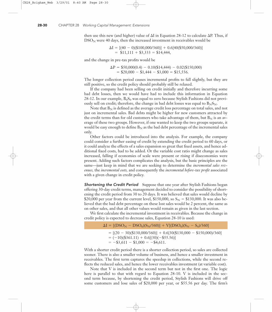
then use this new (and higher) value of �I in Equation 28-12 to calculate �P. Thus, ifDSON were 40 days, then the increased investment in receivables would be

and the change in pre-tax profits would be

The longer collection period causes incremental profits to fall slightly, but they arestill positive, so the credit policy should probably still be relaxed.

If the company had been selling on credit initially and therefore incurring somebad debt losses, then we would have had to include this information in Equation 28-12. In our example, B0S0 was equal to zero because Stylish Fashions did not previ-ously sell on credit; therefore, the change in bad debt losses was equal to BNSN.

Note that BN is defined as the average credit loss percentage on total sales, and notjust on incremental sales. Bad debts might be higher for new customers attracted bythe credit terms than for old customers who take advantage of them, but BN is an av-erage of these two groups. However, if one wanted to keep the two groups separate, itwould be easy enough to define BN as the bad debt percentage of the incremental salesonly.

Other factors could be introduced into the analysis. For example, the companycould consider a further easing of credit by extending the credit period to 60 days, orit could analyze the effects of a sales expansion so great that fixed assets, and hence ad-ditional fixed costs, had to be added. Or the variable cost ratio might change as salesincreased, falling if economies of scale were present or rising if diseconomies werepresent. Adding such factors complicates the analysis, but the basic principles are thesame—just keep in mind that we are seeking to determine the incremental sales rev-enues, the incremental costs, and consequently the incremental before-tax profit associatedwith a given change in credit policy.

Shortening the Credit Period Suppose that one year after Stylish Fashions beganoffering 30-day credit terms, management decided to consider the possibility of short-ening the credit period from 30 to 20 days. It was believed that sales would decline by$20,000 per year from the current level, $150,000, so SN � $130,000. It was also be-lieved that the bad debt percentage on these lost sales would be 2 percent, the same ason other sales, and that all other values would remain as given in the last section.

We first calculate the incremental investment in receivables. Because the change incredit policy is expected to decrease sales, Equation 28-10 is used:

With a shorter credit period there is a shorter collection period, so sales are collectedsooner. There is also a smaller volume of business, and hence a smaller investment inreceivables. The first term captures the speedup in collections, while the second re-flects the reduced sales, and hence the lower receivables investment (at variable cost).

Note that V is included in the second term but not in the first one. The logichere is parallel to that with regard to Equation 28-10. V is included in the sec-ond term because, by shortening the credit period, Stylish Fashions will drive offsome customers and lose sales of $20,000 per year, or $55.56 per day. The firm’s

� �$3,611 � $1,000 � �$4,611.� (�10)($361.11) � 0.6[(30)(�$55.56)]� [(20 � 30)($130,000/360)] � 0.6[30($130,000 � $150,000)/360]

�I � [(DSON � DSO0)(SN/360)] � V[(DSO0)(SN � S0)/360]

� $20,000 � $1,444 � $3,000 � $15,556.�P � $50,000(0.4) � 0.10($14,444) � 0.02($150,000)

� $11,111 � $3,333 � $14,444,�I � [(40 � 0)($100,000/360)] � 0.6[40($50,000/360)]



investment in those sales was only 60 percent of the average receivables outstand-ing, or 0.6(30)($55.56) � $1,000. However, the situation is different for the re-maining customers. They would have paid their full purchase price—variable costplus profit—after 30 days. Now, however, they will have to pay this amount 10 dayssooner, so those funds will be available to meet operating costs or for investment.Thus, the first term should not be reduced by the variable cost factor. Therefore, intotal, reducing the credit period would result in a $4,611 reduction in the invest-ment in receivables, consisting of a $3,611 decline in receivables associated withcontinuing customers and a further $1,000 decline in investment as a result of thereduced sales volume.

With the change in investment calculated, we can now analyze the profitability ofthe proposed change using Equation 28-12:

Since the expected incremental pre-tax profits are negative, the firm should not re-duce its credit period from 30 to 20 days.

Changes in Other Credit Policy Variables

In the preceding section, we examined the effects of changes in the credit period.Changes in other credit policy variables may be analyzed similarly. In general, wewould follow these steps:

Step 1. Estimate the effect of the policy change on sales, on DSO, on bad debt losses,and so on.

Step 2. Determine the change in the firm’s investment in receivables. If the changewill increase sales, then use Equation 28-10 to calculate �I. Conversely, if thechange will decrease sales, then use Equation 28-11.

Step 3. Use Equation 28-12, or one of its variations, to calculate the effect of thechange on pre-tax profits. If profits are expected to increase, the policy changeshould be made, unless it is judged to increase the firm’s risk by a dispropor-tionate amount.

Simultaneous Changes in Policy Variables

In the preceding discussion, we considered the effects of changes in only one creditpolicy variable. The firm could, of course, change several or even all policy variablessimultaneously. An almost endless variety of equations could be developed, dependingon which policy variables are manipulated and on the assumed effects on sales, dis-counts taken, the collection period, bad debt losses, the existence of excess capacity,changes in credit department costs, changes in the variable cost percentage, and so on.The analysis would get “messy,” and the incremental profit equation would be com-plex, but the principles we have developed could be used to handle any type of policychange.

Describe the incremental analysis approach for evaluating a proposed credit pol-icy change.

How can risk be incorporated into the analysis?

� �$8,000 � $461 � $400 � �$7,139.� [(0.02)($130,000) � (0.02)($150,000)] � $0

� ($130,000 � $150,000)(0.4) � 0.10(�$4,611)

�P � (SN � S0)(1 � V) � k(�I) � (BNSN � B0S0) � (DNSNPN � D0S0P0)



Summary� The Baumol model provides insights into the optimal cash balance. The model

balances the opportunity cost of holding cash against the transactions costs associ-ated with obtaining cash either by selling marketable securities or by borrowing.

.

� Firms generally set their target cash balances at the level which holds the risk ofrunning out of cash to some acceptable level. Monte Carlo simulation can behelpful in setting the target cash balance.

� Inventory costs can be divided into three parts: carrying costs, ordering costs, andstock-out costs. In general, carrying costs increase as the level of inventory rises,but ordering costs and stock-out costs decline with larger inventory holdings.

� Total carrying cost (TCC) is equal to the percentage cost of carrying inventory(C) times the purchase price per unit of inventory (P) times the average number ofunits held (A): TCC � (C)(P)(A).

� Total ordering cost (TOC) is equal to the fixed cost of placing an order (F) timesthe number of orders placed per year (N): TOC � (F)(N).

� Total inventory costs (TIC) equal total carrying cost (TCC) plus total orderingcost (TOC): TIC � TCC � TOC.

� The economic ordering quantity (EOQ) model is a formula for determining theorder quantity that will minimize total inventory costs:

Here F is the fixed cost per order, S is annual sales in units, C is the percentage costof carrying inventory, and P is the purchase price per unit.

� The reorder point is the inventory level at which new items must be ordered.� Safety stocks are held to avoid shortages (1) if sales increase more than was ex-

pected or (2) if shipping delays are encountered on inventory ordered. The cost ofcarrying a safety stock, which is separate from that based on the EOQ model, isequal to the percentage cost of carrying inventory times the purchase price perunit times the number of units held as the safety stock.

� Firms can use days sales outstanding (DSO) and aging schedules to help mon-itor their receivables position, but the best way to monitor aggregate receivables isthe payments pattern approach. The primary tool in this approach is the uncol-lected balances schedule.

� If a firm eases its credit policy by lengthening the credit period, relaxing itscredit standards and collection policy, and offering (or raising) its cash discount, itssales should increase. However, its costs will also increase. A firm should ease itscredit policy only if the costs of doing so will be offset by higher expected rev-enues. In general, credit policy changes should be evaluated on the basis of incre-mental profits.

� Changes in credit policy can be analyzed in two ways. First, pro forma incomestatements can be constructed for both the current and the proposed policies.Second, equations can be used to estimate the incremental change in profits re-sulting from a proposed new credit policy.

This chapter concludes our discussion of working capital management and financing.In Part Nine, we discuss several special topics, beginning with derivatives and riskmanagement in Chapter 24.

EOQ � B2(F)(S)(C)(P)

.

Optimal cash infusion � B2(F)(T)k



Questions

Define each of the following terms:a. Baumol modelb. Total carrying cost; total ordering cost; total inventory costsc. Economic ordering quantity (EOQ); EOQ model; EOQ ranged. Reorder point; safety stocke. Aging schedule; days sales outstanding (DSO)f. Payments pattern approach; uncollected balances schedule

Indicate by a �, �, or 0 whether each of the following events would probably cause average an-nual inventory holdings to rise, fall, or be affected in an indeterminate manner:a. Our suppliers change from delivering by train to air freight.b. We change from producing just-in-time to meet seasonal demand to

steady, year-round production.c. Competition in the markets in which we sell increases.d. The general rate of inflation rises.e. Interest rates rise; other things are constant.

Self-Test Problems (Solutions Appear in Appendix A)

The McCue Company expects to have sales of $10 million this year under its current operatingpolicies. Its variable costs as a percentage of sales are 80 percent, and its cost of capital is 16 per-cent. Currently the firm’s credit policy is net 25 (no discount for early payment). However, itsDSO is 30 days, and its bad debt loss percentage is 2 percent. McCue spends $50,000 per yearto collect bad debts, and its federal-plus-state-plus-local tax rate is 50 percent.

The credit manager is considering two alternative proposals, given below, for changing thefirm’s credit policy. Find the expected change in net income, taking into consideration antici-pated changes in carrying costs for accounts receivable, the probable bad debt losses, and thediscounts likely to be taken, for each proposal. Should a change in credit policy be made?

Proposal 1: Lengthen the credit period by going from net 25 to net 30. The bad debt collec-tion expenditures will remain constant. Under this proposal, sales are expected to increase by $1million annually, and the bad debt loss percentage on new sales is expected to rise to 4 percent(the loss percentage on old sales should not change). In addition, the DSO is expected to in-crease from 30 to 45 days on all sales.

Proposal 2: Shorten the credit period by going from net 25 to net 20. Again, collection ex-penses will remain constant. The anticipated effects of this change are (1) a decrease in sales of$1 million per year, (2) a decline in the DSO from 30 to 22 days, and (3) a decline in the baddebt loss percentage to 1 percent on all sales.

The Bertin Breads Company buys and then sells (as bread) 2.6 million bushels of wheat annu-ally. The wheat must be purchased in multiples of 2,000 bushels. Ordering costs, which includegrain elevator removal charges of $3,500, are $5,000 per order. Annual carrying costs are 2 per-cent of the purchase price per bushel of $5. The company maintains a safety stock of 200,000bushels. The delivery time is 6 weeks.a. What is the EOQ?b. At what inventory level should a reorder be placed to prevent having to draw on the safety

stock?c. What are the total inventory costs?d. The wheat processor agrees to pay the elevator removal charges if Bertin Breads will pur-

chase wheat in quantities of 650,000 bushels. Would it be to the firm’s advantage to orderunder this alternative?

ST–1EOQ MODEL

ST–1CREDIT POLICY CHANGES

28–2

28–1

Self-Test Problems 28-33


Problems

The Boyd Corporation has annual credit sales of $1.6 million. Current expenses for the collec-tion department are $35,000, bad debt losses are 1.5 percent, and the days sales outstanding is30 days. The firm is considering easing its collection efforts such that collection expenses will bereduced to $22,000 per year. The change is expected to increase bad debt losses to 2.5 percentand to increase the days sales outstanding to 45 days. In addition, sales are expected to increaseto $1,625,000 per year.

Should the firm relax collection efforts if the opportunity cost of funds is 16 percent, thevariable cost ratio is 75 percent, and taxes are 40 percent?

The Gentry Garden Center sells 90,000 bags of lawn fertilizer annually. The optimal safetystock (which is on hand initially) is 1,000 bags. Each bag costs the firm $1.50, inventory carry-ing costs are 20 percent, and the cost of placing an order with its supplier is $15.a. What is the economic ordering quantity?b. What is the maximum inventory of fertilizer?c. What will be the firm’s average inventory?d. How often must the company order?

Kim Mitchell, the new credit manager of the Vinson Corporation, was alarmed to find that Vin-son sells on credit terms of net 90 days while industrywide credit terms have recently been low-ered to net 30 days. On annual credit sales of $2.5 million, Vinson currently averages 95 days ofsales in accounts receivable. Mitchell estimates that tightening the credit terms to 30 days wouldreduce annual sales to $2,375,000, but accounts receivable would drop to 35 days of sales andthe savings on investment in them should more than overcome any loss in profit.

Vinson’s variable cost ratio is 85 percent, and taxes are 40 percent. If the interest rate onfunds invested in receivables is 18 percent, should the change in credit terms be made?

The Russ Fogler Company, a small manufacturer of cordless telephones, began operations onJanuary 1, 2001. Its credit sales for the first 6 months of operations were as follows:

Month Credit Sales

January $ 50,000February 100,000March 120,000April 105,000May 140,000June 160,000

Throughout this entire period, the firm’s credit customers maintained a constant payments pat-tern: 20 percent paid in the month of sale, 30 percent paid in the month following the sale, and50 percent paid in the second month following the sale.a. What was Fogler’s receivables balance at the end of March and at the end of June?b. Assume 90 days per calendar quarter. What were the average daily sales (ADS) and days sales

outstanding (DSO) for the first quarter and for the second quarter? What were the cumula-tive ADS and DSO for the first half-year?

c. Construct an aging schedule as of June 30. Use 0–30, 31–60, and 61–90 day account ages.d. Construct the uncollected balances schedule for the second quarter as of June 30.

Barenbaum Industries projects that cash outlays of $4.5 million will occur uniformly through-out the year. Barenbaum plans to meet its cash requirements by periodically selling marketablesecurities from its portfolio. The firm’s marketable securities are invested to earn 12 percent,and the cost per transaction of converting securities to cash is $27.a. Use the Baumol model to determine the optimal transaction size for transfers from mar-

ketable securities to cash.b. What will be Barenbaum’s average cash balance?c. How many transfers per year will be required?

28–5OPTIMAL CASH TRANSFER

28–4MONITORING OF RECEIVABLES

28–3TIGHTENING CREDIT TERMS

28–2ECONOMIC ORDERING

QUANTITY

28–1RELAXING COLLECTION

EFFORTS



d. What will be Barenbaum’s total annual cost of maintaining cash balances? What would thetotal cost be if the company maintained an average cash balance of $50,000 or of $0 (it de-posits funds daily to meet cash requirements)?

Spreadsheet Problems

Start with the partial model in the file Ch 28-6 Build a Model.xls from the textbook’s CD-ROM. The following inventory data have been established for the Adler Corporation:

(1) Orders must be placed in multiples of 100 units.(2) Annual sales are 338,000 units.(3) The purchase price per unit is $3.(4) Carrying cost is 20 percent of the purchase price of goods.(5) Cost per order placed is $24.(6) Desired safety stock is 14,000 units; this amount is on hand initially(7) Two weeks are required for delivery.

a. What is the EOQ?b. How many orders should the firm place each year?c. At what inventory level should a reorder be made? [Hint: Reorder point � Safety stock �

(Weeks to deliver � Weekly usage) � Goods in transit.]d. Calculate the total costs of ordering and carrying inventories if the order quantity is (1)

4,000 units, (2) 4,800 units, or (3) 6,000 units. What are the total costs if the order quantityis the EOQ?

e. What are the EOQ and total inventory costs if(1) Sales increase to 500,000 units?(2) Fixed order costs increase to $30? Sales remain at 338,000 units.(3) Purchase price increases to $4? Leave sales and fixed costs at original values.

Start with the file Ch 28-7 What If Analysis.xls and answer the questions shown there.28–7WHAT IF ANALYSIS:

ACCOUNTS RECEIVABLE MANAGEMENT

28–6BUILD A MODEL:

INVENTORY MANAGEMENT

Mini Case 28-35

SECTION I: Receivables Management Rich Jackson, a recent finance graduate, is plan-ning to go into the wholesale building supply business with his brother, Jim, who majored inbuilding construction. The firm would sell primarily to general contractors, and it would startoperating next January. Sales would be slow during the cold months, rise during the spring, andthen fall off again in the summer, when new construction in the area slows. Sales estimates forthe first 6 months are as follows (in thousands of dollars):

January $100 March $300 May $200February 200 April 300 June 100

The terms of sale are net 30, but because of special incentives, the brothers expect 30 per-cent of the customers (by dollar value) to pay on the 10th day following the sale, 50 percent topay on the 40th day, and the remaining 20 percent to pay on the 70th day. No bad debt lossesare expected, because Jim, the building construction expert, knows which contractors are hav-ing financial problems.a. Assume that, on average, the brothers expect annual sales of 18,000 items at an average price

of $100 per item. (Use a 360-day year.)(1) What is the firm’s expected days sales outstanding (DSO)?(2) What is its expected average daily sales (ADS)?(3) What is its expected average accounts receivable level?

CD

CD

CDSee Ch 28 Show.ppt andCh 28 Mini Case.xls.



(4) Assume that the firm’s profit margin is 25 percent. How much of the receivables balancemust be financed? What would the firm’s balance sheet figures for accounts receivable,notes payable, and retained earnings be at the end of 1 year if notes payable are used tofinance the investment in receivables? Assume that the cost of carrying receivables hadbeen deducted when the 25 percent profit margin was calculated.

(5) If bank loans have a cost of 12 percent, what is the annual dollar cost of carrying the re-ceivables?

b. What are some factors which influence (1) a firm’s receivables level and (2) the dollar cost ofcarrying receivables?

c. Assuming that the monthly sales forecasts given previously are accurate, and that customerspay exactly as was predicted, what would the receivables level be at the end of each month?To reduce calculations, assume that 30 percent of the firm’s customers pay in the month of sale, 50percent pay in the month following the sale, and the remaining 20 percent pay in the second monthfollowing the sale. Note that this is a different assumption than was made earlier. Use the follow-ing format to answer parts c and d:

Quarterly

Month Sales End-of-Month Receivables Sales ADS DSO � (A/R)(ADS)

Jan $100 $ 70Feb 200 160Mar 300 250 $600 $6.67 37.5Apr $300May 200Jun 100

d. What is the firm’s forecasted average daily sales for the first 3 months? For the entire half-year? The days sales outstanding is commonly used to measure receivables performance.What DSO is expected at the end of March? At the end of June? What does the DSO indi-cate about customers’ payments? Is DSO a good management tool in this situation? If not,why not?

e. Construct aging schedules for the end of March and the end of June (use the format givenbelow). Do these schedules properly measure customers’ payment patterns? If not, why not?

March June

Age of Account (Days) A/R % A/R %

0–30 $210 84%31–60 40 1661–90 0 0

$250 100%

f. Construct the uncollected balances schedules for the end of March and the end of June. Usethe format given below. Do these schedules properly measure customers’ payment patterns?

March June

Contribution A/R-to- Contribution A/R-to-Month Sales to A/R Sales Ratio Month Sales to A/R Sales Ratio

Jan $100 $ 0 0% AprFeb 200 40 20 MayMar 300 210 70 June


Mini Case 28-37

g. Assume that it is now July of Year 1, and the brothers are developing pro forma financialstatements for the following year. Further, assume that sales and collections in the firsthalf-year matched the predicted levels. Using the Year 2 sales forecasts as shown next,what are next year’s pro forma receivables levels for the end of March and for the end ofJune?

Predicted A/R-to- Predicted ContributionMonth Predicted Sales Sales Ratio to Receivables

Jan $150 0% $ 0Feb 300 20 60Mar 500 70 350

Projected March 31 A/R balance � $410

Apr $400May 300Jun 200

Projected June 30 A/R balance �

h. Assume now that it is several years later. The brothers are concerned about the firm’s cur-rent credit terms, which are now net 30, which means that contractors buying buildingproducts from the firm are not offered a discount, and they are supposed to pay the fullamount in 30 days. Gross sales are now running $1,000,000 a year, and 80 percent (by dol-lar volume) of the firm’s paying customers generally pay the full amount on Day 30, whilethe other 20 percent pay, on average, on Day 40. Two percent of the firm’s gross sales endup as bad debt losses.

The brothers are now considering a change in the firm’s credit policy. The changewould entail (1) changing the credit terms to 2/10, net 20, (2) employing stricter creditstandards before granting credit, and (3) enforcing collections with greater vigor than inthe past. Thus, cash customers and those paying within 10 days would receive a 2 percentdiscount, but all others would have to pay the full amount after only 20 days. The broth-ers believe that the discount would both attract additional customers and encourage someexisting customers to purchase more from the firm—after all, the discount amounts to aprice reduction. Of course, these customers would take the discount and, hence, would payin only 10 days. The net expected result is for sales to increase to $1,100,000; for 60 per-cent of the paying customers to take the discount and pay on the 10th day; for 30 percentto pay the full amount on Day 20; for 10 percent to pay late on Day 30; and for bad debtlosses to fall from 2 percent to 1 percent of gross sales. The firm’s operating cost ratio willremain unchanged at 75 percent, and its cost of carrying receivables will remain unchangedat 12 percent.

To begin the analysis, describe the four variables which make up a firm’s credit policy, and ex-plain how each of them affects sales and collections. Then use the information given in part h toanswer parts i through n.

i. Under the current credit policy, what is the firm’s days sales outstanding (DSO)? Whatwould the expected DSO be if the credit policy change were made?

j. What is the dollar amount of the firm’s current bad debt losses? What losses would be ex-pected under the new policy?

k. What would be the firm’s expected dollar cost of granting discounts under the new policy?l. What is the firm’s current dollar cost of carrying receivables? What would it be after the

proposed change?m. What is the incremental after-tax profit associated with the change in credit terms? Should

the company make the change? (Assume a tax rate of 40 percent.)



New Old Difference

Gross sales $1,000,000Less discounts 0

Net sales $1,000,000Production costs 750,000

Profit before credit costs and taxes $ 250,000

New Old Difference

Credit-related costs:Carrying costs 8,000Bad debt losses 20,000

Profit before taxes $ 222,000Taxes (40%) 88,800Net income $ 133,200

n. Suppose the firm makes the change, but its competitors react by making similar changes totheir own credit terms, with the net result being that gross sales remain at the current$1,000,000 level. What would the impact be on the firm’s post-tax profitability?

SECTION II: Inventory Management Andria Mullins, financial manager of Webster Elec-tronics, has been asked by the firm’s CEO, Fred Weygandt, to evaluate the company’s inventorycontrol techniques and to lead a discussion of the subject with the senior executives. Andriaplans to use as an example one of Webster’s “big ticket” items, a customized computer mi-crochip that the firm uses in its laptop computer. Each chip costs Webster $200, and in additionit must pay its supplier a $1,000 setup fee on each order. Further, the minimum order size is 250units; Webster’s annual usage forecast is 5,000 units; and the annual carrying cost of this item isestimated to be 20 percent of the average inventory value.

Andria plans to begin her session with the senior executives by reviewing some basic inven-tory concepts, after which she will apply the EOQ model to Webster’s microchip inventory. Asher assistant, you have been asked to help her by answering the following questions:a. Why is inventory management vital to the financial health of most firms?b. What assumptions underlie the EOQ model?c. Write out the formula for the total costs of carrying and ordering inventory, and then use

the formula to derive the EOQ model.d. What is the EOQ for custom microchips? What are total inventory costs if the EOQ is or-

dered?e. What is Webster’s added cost if it orders 400 units at a time rather than the EOQ quantity?

What if it orders 600 per order?f. Suppose it takes 2 weeks for Webster’s supplier to set up production, make and test the

chips, and deliver them to Webster’s plant. Assuming certainty in delivery times and usage,at what inventory level should Webster reorder? (Assume a 52-week year, and assume thatWebster orders the EOQ amount.)

g. Of course, there is uncertainty in Webster’s usage rate as well as in delivery times, so thecompany must carry a safety stock to avoid running out of chips and having to halt produc-tion. If a 200-unit safety stock is carried, what effect would this have on total inventorycosts? What is the new reorder point? What protection does the safety stock provide if us-age increases, or if delivery is delayed?

h. Now suppose Webster’s supplier offers a discount of 1 percent on orders of 1,000 or more.Should Webster take the discount? Why or why not?

i. For many firms, inventory usage is not uniform throughout the year, but, rather, followssome seasonal pattern. Can the EOQ model be used in this situation? If so, how?

j. How would these factors affect an EOQ analysis?(1) The use of just-in-time procedures.(2) The use of air freight for deliveries.


Selected Additional References and Cases 28-39

Selected Additional References and Cases

Key references on cash balance models include the following:Daellenbach, Hans G., “Are Cash Management Optimiza-

tion Models Worthwhile?” Journal of Financial and Quan-titative Analysis, September 1974, 607–626.

Miller, Merton H., and Daniel Orr, “The Demand forMoney by Firms: Extension of Analytic Results,” Journalof Finance, December 1968, 735–759.

Mullins, David Wiley, Jr., and Richard B. Homonoff, “Ap-plications of Inventory Cash Management Models,” inModern Developments in Financial Management, Stewart C.Myers, ed. (New York: Praeger, 1976).

Stone, Bernell K., “The Use of Forecasts for Smoothing inControl-Limit Models for Cash Management,” FinancialManagement, Spring 1972, 72–84.

The following cases from the Cases in Financial Management:Dryden Request series focus on the credit policy decision:Case 33, “Upscale Toddlers, Inc.,” Case 50, “Mitchell Lum-

ber Co.,” and Case 62, “Western Supply,” which dealwith credit policy changes.

Case 34, “Texas Rose Company,” and Case 34A, “Bridgewa-ter Pool Company,” which focus on receivables manage-ment.

(3) The use of a computerized inventory control system, wherein as units were removedfrom stock, an electronic system automatically reduced the inventory account and, whenthe order point was hit, automatically sent an electronic message to the supplier placingan order. The electronic system ensures that inventory records are accurate, and that or-ders are placed promptly.

(4) The manufacturing plant is redesigned and automated. Computerized process equip-ment and state-of-the-art robotics are installed, making the plant highly flexible in thesense that the company can switch from the production of one item to another at a min-imum cost and quite quickly. This makes short production runs more feasible than underthe old plant setup.


Brian F Shannon

Copyright (C) 2001 by Harcourt,Inc.

Working Capital Management: Extensions - Cengage

Documents

Transcript of Working Capital Management: Extensions - Cengage