University of Tennessee, Knoxville University of Tennessee, Knoxville

TRACE: Tennessee Research and Creative TRACE: Tennessee Research and Creative

Exchange Exchange

Doctoral Dissertations Graduate School

5-2017

Computational Thermal-Hydraulics Modeling of Twisted Tape Computational Thermal-Hydraulics Modeling of Twisted Tape

Enabled High Heat Flux Components Enabled High Heat Flux Components

Emily Buckman Clark University of Tennessee, Knoxville, ebuckman@vols.utk.edu

Follow this and additional works at: https://trace.tennessee.edu/utk_graddiss

Part of the Aerodynamics and Fluid Mechanics Commons, Energy Systems Commons, Heat Transfer,

Combustion Commons, Nuclear Engineering Commons, and the Other Aerospace Engineering Commons

Recommended Citation Recommended Citation Clark, Emily Buckman, "Computational Thermal-Hydraulics Modeling of Twisted Tape Enabled High Heat Flux Components. " PhD diss., University of Tennessee, 2017. https://trace.tennessee.edu/utk_graddiss/4393

This Dissertation is brought to you for free and open access by the Graduate School at TRACE: Tennessee Research and Creative Exchange. It has been accepted for inclusion in Doctoral Dissertations by an authorized administrator of TRACE: Tennessee Research and Creative Exchange. For more information, please contact trace@utk.edu.

To the Graduate Council:

I am submitting herewith a dissertation written by Emily Buckman Clark entitled "Computational

Thermal-Hydraulics Modeling of Twisted Tape Enabled High Heat Flux Components." I have

examined the final electronic copy of this dissertation for form and content and recommend

that it be accepted in partial fulfillment of the requirements for the degree of Doctor of

Philosophy, with a major in Energy Science and Engineering.

Arnold Lumsdaine, Kivanc Ekici, Major Professor

We have read this dissertation and recommend its acceptance:

Arthur Ruggles, David Donovan

Accepted for the Council:

Dixie L. Thompson

Vice Provost and Dean of the Graduate School

(Original signatures are on file with official student records.)

Computational Thermal-Hydraulics Modeling of Twisted Tape Enabled High Heat Flux Components

A Dissertation Presented for the Doctor of Philosophy

Degree The University of Tennessee, Knoxville

Emily Buckman Clark May 2017

ii

Copyright © 2017 by Emily Buckman Clark All rights reserved.

iii

To my husband, John, for your unwavering support and confidence in me. I can’t wait to start our next adventure.

To my parents, Diana and Mitch, for always believing in me and pushing me to succeed. You showed me the drive to make this possible.

iv

Acknowledgements This accomplishment would not have been possible without the support of a great number

of people. Thank you to my advisors Dr. Kivanc Ekici and Dr. Arnold Lumsdaine. Thank you

to Dr. Ekici for supporting me throughout my whole graduate school experience. He saw

the potential in me and gave me the opportunities to make me the researcher and engineer

that I am today. Thank you to Dr. Lumsdaine for bringing me into the world of fusion

energy. He showed me that I can be flexible with my skills and taught me how to approach

a problem even if I know nothing about it. I would also like to thank Dr. Art Ruggles for his

mentorship and guidance. He showed me the value of a questioning attitude and instilled

the importance of driving towards a goal.

I wouldn’t be where I am today without the Bredesen Center. Thank you to Dr. Lee

Riedinger for bringing me into the family and giving me the opportunity to pursue this

work. Joining the Bredesen Center was the best decision of my graduate career. The

Bredesen Center opened my eyes to the wide world of possibilities that scientists can

achieve. It not only taught me how to communicate effectively with both scientists and the

public but also why it’s important to do so. The Bredesen Center showed me the

importance of looking at the bigger picture, and I know that perspective will be invaluable

in my career.

I would also like to thank those who supported my work at Oak Ridge National

Laboratory in the Fusion and Materials for Nuclear Systems Division. Thank you to Phil

Ferguson and Gary Bell for supporting me as I developed my skills. Thank you to Jean

Boscary for his collaboration and guidance on this work. Furthermore, thank you to the

Office of Fusion Energy Sciences, which generously funded this collaboration with the

Wendelstein 7-X experiment.

Lastly, this work would not have been possible without the support of my closest

friends. Thank you to Jordan Sawyer, Zeke Stannard, and Michael Merriweather. As we

continue our careers and move apart, I know we’ll always be “BEFFs.” Thank you to

Guinevere Shaw for our countless hours of discussion and laughter. Your passion and drive

v

are inspirational. Thank you to Mark Christian for our brainstorming sessions and

discussions. I know you will meet your goals. Finally, thank you to Kate Manz and Reed

Wittman. From football games to dinner parties, we always had a great time and a ton of

laughs. I can’t wait to see where your careers take you. Friends are the family we choose for

ourselves, and the Clarks choose all of you.

vi

Abstract

The goal of this work was to perform a computational investigation into the thermal-

hydraulic performance of water-cooled, twisted tape enabled high heat flux components at

fusion relevant conditions. Fusion energy is a promising option for future clean energy

generation, but the community must overcome significant scientific and engineering

challenges before meeting the goal of electricity generation. One such challenge is the high

heat flux thermal management of components in fusion and plasma physics experiments.

Plasma facing components in the magnetic confinement devices, such as ITER or W7-X, will

be subjected to extreme heat loads on the order of 10-20 MW/m2. The heat dissipation

issue will become critical as these next generations of experiments come online, and active

cooling will be necessary to decrease the thermal loading and prevent failure of the

components.

Single-phase computational modeling was performed with the ANSYS CFX software to

investigate the performance of water-cooled twisted tape devices. Computational

investigations were first performed for a general geometry at moderate conditions and

were then ramped up to fusion relevant conditions. This work resulted in a wide range of

topics including comparisons to experiments and legacy correlations, comparisons of

various turbulence models, investigations into local information, a parametric sweep of

different tape characteristics, and identification of future opportunities.

Key results stemmed from the investigation into the local flow field. The work revealed

characteristics of twisted tape enabled swirl flow, which has not yet been noted in the

literature. Secondary circulation resulted in so-called “inflow” regions, where the boundary

layer was reinjected into the freestream. At moderate, uniform heating conditions, these

regions were shown to correspond to regions of low wall shear stress, low heat transfer

coefficients, and high surface temperatures making them candidates for early burnout.

Investigation of wall shear stress contours revealed apparent “striping” that develops in

twisted tape induced swirl flow due to the secondary circulation. While these key

qualitative features were still noted in the fusion relevant investigation, the connection

vii

between the inflow regions and surface temperature was concluded to be minimal under

one-sided, high heat flux conditions.

viii

Table of Contents

1. Introduction ...................................................................................................................................................... 1

2. Background ........................................................................................................................................................ 4

2.1. Twisted Tape Background .................................................................................................................. 4

2.2. Current Status of Twisted Tape Research .................................................................................... 5

2.2.1. Experimental Works .................................................................................................................... 5

Development of Thermal-Hydraulic Correlations ................................................................... 5

One-Sided Heating Experiments .................................................................................................... 6

Flow Visualization Experiments .................................................................................................... 7

2.2.2. Computational Works ................................................................................................................ 8

Classical Twisted Tape Inserts ........................................................................................................ 8

Modified Twisted Tape Inserts ....................................................................................................... 9

Motivation for Current Study ........................................................................................................13

3. Overview of the Computational Approach .........................................................................................15

3.1. Governing Equations ..........................................................................................................................15

3.2. Turbulence Modeling ..........................................................................................................................16

3.3. Selection of Turbulence Models .....................................................................................................18

3.3.1. The Standard k-epsilon Model ...............................................................................................18

3.3.2. The Renormalized Group k-epsilon Model .......................................................................19

3.3.3. The Shear Stress Transport Model ......................................................................................19

3.3.4. The Curvature Correction Method .......................................................................................20

3.4. Modeling in the Near Wall Region .................................................................................................20

3.4.1. Description of the Near Wall Region ...................................................................................20

3.4.2. Turbulence Modeling Near the Wall ...................................................................................21

Scalable Wall Functions in CFX ....................................................................................................22

Automatic Near Wall Treatment in CFX ...................................................................................24

Temperature in the Near Wall Region ......................................................................................24

4. Computational Investigation for a Tube Equipped with a Twisted Tape ................................26

4.1. Computational Models .......................................................................................................................26

ix

4.1.1. Adiabatic Investigation .............................................................................................................26

Adiabatic Model Geometry ............................................................................................................26

Adiabatic Conditions ........................................................................................................................28

4.1.2. Diabatic Investigation ...............................................................................................................29

Diabatic Model Geometry ...............................................................................................................29

Diabatic Conditions ..........................................................................................................................30

4.2. Computational Validation .................................................................................................................34

4.2.1. Adiabatic Validation ..................................................................................................................34

Calculations and Legacy Friction Factor Correlations ........................................................34

Experimental Ranges of the Legacy Friction Factor Correlations ...................................35

Comparison of Adiabatic Global Parameters to Legacy Works ........................................36

Comparison to Adiabatic Flow Visualization Experiments ................................................38

4.2.2. Diabatic Validation .....................................................................................................................43

Calculations and Legacy Nusselt Number Correlations .......................................................43

Experimental Ranges of the Legacy Nusselt Number Correlations .................................45

Comparison of Diabatic Global Parameters to Legacy Works ..........................................47

4.3. Investigation of Local Flow Information .....................................................................................51

4.3.1. Adiabatic Investigation into Local Flow Information ...................................................51

Adiabatic Flow Patterns .................................................................................................................51

Further Investigation into Inflow Regions ...............................................................................54

Transient Studies for Further Mesh Refinement ....................................................................57

4.3.2. Diabatic Investigation into Local Flow Information .....................................................62

Diabatic Flow Patterns and Temperature Contours .............................................................62

Further Investigation of Inflow Regions ...................................................................................65

4.4. Selection of Turbulence Model .......................................................................................................71

4.5. Summary of Key Conclusions ..........................................................................................................74

5. Parametric Study for Various Twist Ratios .........................................................................................76

5.1. Model Geometry and Setup ..............................................................................................................76

5.2. Effect of Twist Ratio on Global Parameters ...............................................................................78

x

5.3. Comparison of Global Parameters to Legacy Works ..............................................................78

5.3.1. Comparison to Legacy Thermal-Hydraulic Correlations ............................................78

5.3.2. Comparison to Legacy Experimental Data ........................................................................80

5.4. Investigation into Local Flow Information ................................................................................85

5.4.1. Flow Patterns and Temperature Contours .......................................................................85

5.4.2. Further Investigation of Inflow Regions ............................................................................88

5.5. Summary of Key Conclusions ..........................................................................................................99

6. Computational Investigation at Fusion Relevant Conditions .................................................... 101

6.1. Monoblock Plasma Facing Components ................................................................................... 101

6.2. Computational Model ...................................................................................................................... 103

6.2.1. Monoblock Model Geometry ............................................................................................ 103

6.2.2. Fusion Relevant Conditions .............................................................................................. 106

6.2.3. Post-Processing Method ..................................................................................................... 110

6.3. Comparison to Prototype Testing .............................................................................................. 114

6.3.1. Initial Comparison ................................................................................................................ 114

6.3.2. Further Investigation of Results ..................................................................................... 114

6.4. Analysis of Local Flow Information ........................................................................................... 120

6.4.1. Flow Patterns and Temperature Contours ................................................................. 122

6.4.2. Further Investigation of Inflow Regions ...................................................................... 126

6.5. Discussion of Local Relationships at Fusion Relevant Conditions ................................. 130

6.5.1. Full Contour Comparison ................................................................................................... 130

6.5.2. Investigation of IAPWS Water Properties ................................................................... 133

6.5.3. Investigation of Near Wall Behavior ............................................................................. 136

6.5.4. Analysis of Local Flow Information at Lower Peak Heat Fluxes ........................ 142

6.6. Investigation of Discrepancies from CFC Prototype Testing ........................................... 145

6.6.1. Investigation of Non-Uniform Thermal Contact Resistance ................................ 146

6.6.2. Investigation of CFC Fiber Misalignment .................................................................... 150

6.7. Summary of Key Conclusions ....................................................................................................... 152

7. Conclusions ................................................................................................................................................... 155

xi

7.1. Summary of the Work ..................................................................................................................... 155

7.2. Key Conclusions ................................................................................................................................. 156

7.2.1. Summary for a Tube Equipped with a Twisted Tape Insert ................................ 156

7.2.2. Summary for a Monoblock Geometry at Fusion Relevant Conditions ............. 158

7.3. Opportunities for Future Work ................................................................................................... 159

References ......................................................................................................................................................... 161

Vita ........................................................................................................................................................................ 170

xii

List of Tables

Table 2.1: Variety of twisted tape (TT) geometries and turbulence models in the

computational literature ...................................................................................................................14

Table 4.1: Diabatic cases investigated .......................................................................................................32

Table 4.2: Legacy Fanning friction factor correlations for isothermal conditions as cited in

Ref. [8] ......................................................................................................................................................35

Table 4.3: Experimental parameters for legacy friction factor correlations ..............................36

Table 4.4: Legacy Nusselt number correlations .....................................................................................44

Table 4.5: Experimental parameters for legacy correlations ...........................................................46

Table 4.6: Three axial locations selected for local flow investigation ...........................................52

Table 4.7: Cut plane locations for wall shear stress contours ..........................................................56

Table 4.8: Mesh statistics and runtimes for mesh refinement studies .........................................58

Table 5.1: Axial locations selected for the local flow investigation ................................................86

Table 6.1: Material properties implemented for solid components [75-80] ........................... 109

Table 6.2: Peak temperature values in domains of interest for all PHF .................................... 118

Table 6.3: Axial locations selected for the fusion relevant local flow investigation ............. 123

Table 6.4: Peak water temperature for the monoblock model ..................................................... 134

xiii

List of Figures Figure 2.1: Twisted tape geometric characteristics from Ref. [12] .................................................. 5

Figure 2.2: Modified twisted tape inserts with surface or geometry modifications including

the (a) perforated twisted tape [28], (b) notched twisted tape [28], (c) jagged

twisted tape [28], (d) triangular cut twisted tape [33, 34], and (e) edgefold twisted

tape [31] ..................................................................................................................................................10

Figure 4.1: Adiabatic validation model geometry .................................................................................27

Figure 4.2: Applied heat flux of 1 MW/m2 where LH is the heated section, LC is the calming

section, and Lent is the straight entrance region [11] .............................................................31

Figure 4.3: Fanning friction factor comparison of computational results and legacy

correlations [13-16, 22] ....................................................................................................................37

Figure 4.4: Adiabatic Fanning friction factor comparison of simulated results (CFX) and the

Manglik and Bergles correlation (MB) [15] ...............................................................................39

Figure 4.5: Comparison of (a) computational axial velocity contour to (b) experimental flow

measurements of Smithberg and Landis [23] ..........................................................................42

Figure 4.6: Comparison of (a) computational axial velocity contour to (b) experimental flow

measurements of Seymour [22] .....................................................................................................42

Figure 4.7: Diabatic Fanning friction factor comparison of simulated results (CFX) and the

Manglik and Bergles correlation (MB) [15] for heat fluxes of 0.5 MW/m2 (left) and 1

MW/m2 (right) ......................................................................................................................................48

Figure 4.8: Nusselt number comparison of simulated results (CFX) and the Manglik and

Bergles correlation (MB) [15] for heat fluxes of 0.5 MW/m2 (left) and 1 MW/m2

(right) .......................................................................................................................................................50

Figure 4.9: Nusselt number comparison of simulated results to legacy correlations [14-17]

for heat fluxes of 0.5 MW/m2 (left) and 1 MW/m2 (right) ..................................................50

Figure 4.10: (a) Total velocity contour and (b) tangential velocity projection (Re=8x104, k-

eps) ............................................................................................................................................................52

xiv

Figure 4.11: Comparison of total velocity contours as the flow moves downstream

(Re=8x104, k-eps) ................................................................................................................................52

Figure 4.12: Comparison of total velocity contours for various turbulence models at a plane

near the exit region (Plane 3, Re=8x104) ...................................................................................53

Figure 4.13: Wall shear stress for standard turbulence models along the outer perimeter at

a plane near the exit region (Plane 3 in Table 4.6, Re=8x104) ...........................................55

Figure 4.14: Wall shear stress for curvature correction (CC) turbulence models along the

outer perimeter at a plane near the exit region (Plane 3 in Table 4.6, Re=8x104) ....55

Figure 4.15: Adiabatic wall shear stress contours where cut plane locations are shown in

Table 4.7 (Re=8x104, k-eps) ............................................................................................................56

Figure 4.16: Mesh resolutions utilized for refinement study including (a) converged steady

state (SS), (b) first transient refinement (TC1), and (c) second transient refinement

(TC2) .........................................................................................................................................................58

Figure 4.17: Comparison of total velocity contours for (a) SS, (b) TC1, and (c) TC2 at a plane

near the exit region .............................................................................................................................60

Figure 4.18: Comparison of total velocity contours for (a) TC1 and (b) TC2 at three axial

locations ..................................................................................................................................................60

Figure 4.19: RMS wall shear stress contours for transient solution where cut plane

locations are shown in Table 4.7 (TC1, Re=8x104, k-eps) ...................................................61

Figure 4.20: Instantaneous wall shear stress contours for transient solution where cut

plane locations are shown in Table 4.7 (TC1, t=10 s, Re=8x104, k-eps) ........................61

Figure 4.21: Comparison of diabatic total velocity contours as the flow moves downstream

(Re=8x104, 𝑞′′=1 MW/m2, k-eps) ..................................................................................................63

Figure 4.22: Comparison of diabatic total velocity contours for various turbulence models

at a plane near the exit region (Plane 3 in Table 4.6, Re=8x104, 𝑞′′=1 MW/m2) ........64

Figure 4.23: Comparison of temperature contours as the flow moves downstream

(Re=8x104, 𝑞′′=1 MW/m2, k-eps) ..................................................................................................64

Figure 4.24: Comparison of temperature contours for various turbulence models at a plane

near the exit region (Plane 3 in Table 4.6, Re=8x104, 𝑞′′=1 MW/m2) .............................66

xv

Figure 4.25: (a) Total velocity and (b) temperature contours at a plane near the exit region

(Plane 3 in Table 4.6, Re=1.5x105, 𝑞′′=1 MW/m2, k-eps) .....................................................66

Figure 4.26: Comparison of wall shear stress and wall heat flux along the upper perimeter

at a plane near the exit region (Plane 3 in Table 4.6, Re=1.5x105, 𝑞′′=1 MW/m2, k-

eps) ............................................................................................................................................................68

Figure 4.27: Comparison of wall shear stress and heat transfer coefficient along the upper

perimeter at a plane near the exit region (Plane 3 in Table 4.6, Re=1.5x105, 𝑞′′=1

MW/m2, k-eps) .....................................................................................................................................68

Figure 4.28: Comparison of wall shear stress and surface temperature along the upper

perimeter at a plane near the exit region (Plane 3 in Table 4.6, Re=1.5x105, 𝑞′′=1

MW/m2, k-eps) .....................................................................................................................................69

Figure 4.29: Comparison of (a) wall heat flux, (b) heat transfer coefficient, (c) wall shear

stress, and (d) surface temperature for standard turbulence models at a plane near

the exit (Plane 3 in Table 4.6, Re=1.5x105, 𝑞′′=1 MW/m2) .................................................70

Figure 4.30: Diabatic wall shear stress contours for various turbulence models where cut

plane locations are shown in Table 4.7 (Re=1.5x105, 𝑞′′=1 MW/m2) .............................72

Figure 5.1: Twisted tape geometries at various twist ratios ............................................................77

Figure 5.2: Effect of twist ratio on the Fanning friction factor for various Reynolds numbers

and heat fluxes ......................................................................................................................................79

Figure 5.3: Effect of twist ratio on the Nusselt number for various Reynolds numbers and

heat fluxes ...............................................................................................................................................79

Figure 5.4: Fanning friction factor comparison of simulation results to legacy correlations

[13-16, 22] for various twist ratios across multiple heat fluxes and Reynolds

numbers ..................................................................................................................................................81

Figure 5.5: Nusselt number comparison of simulation results to legacy correlations [14-17]

for various twist ratios across multiple heat fluxes and Reynolds numbers ...............82

Figure 5.6: Ratio of the swirl to the equivalent axial Nusselt number compared to the

experimental data of Ref. [17] ........................................................................................................83

xvi

Figure 5.7: Ratio of the isothermal swirl flow friction factor to the axial friction factor

compared to experimental data as cited in Ref. [14][13, 14, 22, 23, 63, 64] ................86

Figure 5.8: Comparison of diabatic total velocity contours as the flow moves downstream

for various twist ratios (Re=8x104, 𝑞′′=1 MW/m2) ................................................................87

Figure 5.9: Comparison of temperature contours as the flow moves downstream

(Re=8x104, 𝑞′′=1 MW/m2, y=2) .....................................................................................................89

Figure 5.10: Comparison of temperature contours for various twist ratios at a plane near

the exit region (Plane 3 in Table 5.1, Re=8x104, 𝑞′′=1 MW/m2) .......................................89

Figure 5.11: Total velocity (top) and temperature (bottom) contours at a plane near the

exit region (Plane 3 in Table 5.1, Re=1.5x105, 𝑞′′=1 MW/m2) ...........................................90

Figure 5.12: Wall heat flux for various twist ratios at a plane near the exit region (Plane 3 in

Table 5.1, Re=1.5x105, 𝑞′′=1 MW/m2) .........................................................................................92

Figure 5.13: Heat transfer coefficient for various twist ratios at a plane near the exit region

(Plane 3 in Table 5.1, Re=1.5x105, 𝑞′′=1 MW/m2) ..................................................................93

Figure 5.14: Wall shear stress for various twist ratios at a plane near the exit region (Plane

3 in Table 5.1, Re=1.5x105, 𝑞′′=1 MW/m2) ................................................................................94

Figure 5.15: Surface temperature for various twist ratios at a plane near the exit region

(Plane 3 in Table 5.1, Re=1.5x105, 𝑞′′=1 MW/m2) ..................................................................96

Figure 5.16: Wall shear stress contours for various twist ratios where cut plane locations

are shown in Table 4.7 (Re=1.5x105, 𝑞′′=1 MW/m2) ............................................................97

Figure 5.17: Wall shear stress contour for the straight tape case near the exit region

(Re=1.5x105, 𝑞′′=1 MW/m2) ...........................................................................................................98

Figure 6.1: Computer-aided drawing (CAD) of a W7-X monoblock plasma facing component

prototype with (a) side and (b) axial viewpoints ................................................................ 102

Figure 6.2: W7-X divertor region with scraper element [3] ........................................................... 104

Figure 6.3: Scraper element flow sequence illustration [3] ........................................................... 104

Figure 6.4: CFC monoblock geometry implemented in CFX ........................................................... 105

Figure 6.5: Gaussian heat flux profile applied to a monoblock finger [74] .............................. 108

Figure 6.6: Temperature dependent thermal conductivity of CFC NB31 [74] ........................ 108

xvii

Figure 6.7: Axial and close-up side view of the implemented mesh for the CFC monoblock

geometry .............................................................................................................................................. 111

Figure 6.8: Infrared image of the monoblock prototype at PHF of 20 MW/m2 as seen in Ref.

[53] ......................................................................................................................................................... 112

Figure 6.9: Points for post-processing simulations [74] ................................................................. 112

Figure 6.10: Angular coordinate for monoblock geometry circumferential

distributions ....................................................................................................................................... 113

Figure 6.11: Comparison of experimental [53] and CFX results at the center of the

monoblock ........................................................................................................................................... 115

Figure 6.12: Comparison of experimental [53] and CFX results at the edges of the

monoblock ........................................................................................................................................... 115

Figure 6.13: Temperature contours of computational domains including the (a) CFC, (b)

AMC® copper interlayer, (c) CuCrZr tube, and (d) water for a PHF of 10.5

MW/m2 ................................................................................................................................................. 116

Figure 6.14: Circumferential temperature distributions for various PHF on the monoblock

geometry .............................................................................................................................................. 118

Figure 6.15: Monoblock temperature distributions for (a) Ref. [64] and (b) the current

study at the location of PHF for 10.5 MW/m2 ....................................................................... 119

Figure 6.16: Expected boiling regions for PHF of (a) 10.5 MW/m2, (b) 15 MW/m2, and (c)

20 MW/m2 ........................................................................................................................................... 121

Figure 6.17: (a) Total velocity contour and (b) tangential velocity projection for PHF=10.5

MW/m2 ................................................................................................................................................. 123

Figure 6.18: Comparison of total velocity contours as the flow moves downstream for the

monoblock geometry (PHF=10.5 MW/m2) ............................................................................ 124

Figure 6.19: Comparison of total velocity and temperature contours under the location of

PHF (Plane CB) and near the exit (Plane 3) for the monoblock geometry (PHF=10.5

MW/m2) ............................................................................................................................................... 125

Figure 6.20: Wall shear stress contours for the monoblock geometry ...................................... 127

xviii

Figure 6.21: Comparison of wall shear stress and wall heat flux along the water-tube

interface at the location of PHF (Plane CB in Table 6.3, PHF=10.5 MW/m2) ............ 128

Figure 6.22: Comparison of wall shear stress and HTC along the water-tube interface at the

location of PHF (Plane CB in Table 6.3, PHF=10.5 MW/m2) ............................................ 128

Figure 6.23: Comparison of wall shear stress and surface temperature along the water-tube

interface at the location of PHF (Plane CB in Table 6.3, PHF=10.5 MW/m2) ............ 129

Figure 6.24: Close-up view of the peak surface temperature along the water-tube interface

at the location of PHF (Plane CB in Table 6.3, PHF=10.5 MW/m2) ............................... 131

Figure 6.25: Comparison of wall shear stress and surface temperature along the water-tube

interface near the exit region (Plane 3 in Table 6.3, PHF=10.5 MW/m2) ................... 131

Figure 6.26: Comparison of wall shear stress, wall heat flux, and surface temperature for

the full water domain from the monoblock geometry (Top down viewpoint) ........ 132

Figure 6.27: Water property regimes for the IAPWS IF-97 formulation as implemented in

ANSYS CFX [42, 54] .......................................................................................................................... 134

Figure 6.28: IAPWS water properties in the subcooled water regime ...................................... 135

Figure 6.29: Sampling line utilized in near wall investigation ...................................................... 136

Figure 6.30: Total velocity profiles in the near wall region at three axial locations as given

in Table 6.3 .......................................................................................................................................... 137

Figure 6.31: Temperature profiles in the near wall region at three axial locations as given in

Table 6.3 ............................................................................................................................................... 138

Figure 6.32: Non-dimensional velocity profile in the near wall region ..................................... 140

Figure 6.33: Non-dimensional temperature profile in the near wall region ........................... 141

Figure 6.34: Water temperature contours for lower applied PHF of (a) 1 MW/m2 and (b) 5

MW/m2 ................................................................................................................................................. 143

Figure 6.35: Comparison of wall shear stress and wall heat flux along the water-tube

interface at the location of PHF (Plane CB in Table 6.3, PHF=1 MW/m2) .................. 143

Figure 6.36: Comparison of wall shear stress and HTC along the water-tube interface at the

location of PHF (Plane CB in Table 6.3, PHF=1 MW/m2) .................................................. 144

xix

Figure 6.37: Comparison of wall shear stress and surface temperature along the water-tube

interface at the location of PHF (Plane CB in Table 6.3, PHF=1 MW/m2) .................. 144

Figure 6.38: Implemented non-uniform TCR on the armor-interlayer interface [74] ........ 148

Figure 6.39: Comparison of experimental [53] and CFX results at the center of the

monoblock for a parametric investigation of the TCR [74] .............................................. 148

Figure 6.40: Comparison of experimental [53] and CFX results at the edges of the

monoblock for a parametric investigation of the TCR [74] .............................................. 149

Figure 6.41: Circumferential temperature distributions at the location of peak heat flux for

a parametric investigation of the TCR [74] ............................................................................ 149

Figure 6.42: Rotated coordinate frame for CFC thermal properties in investigation of fiber

misalignment [74] ............................................................................................................................ 151

Figure 6.43: Surface temperature for rotated CFC fibers (φ=8.5°) with a PHF of 10.5

MW/m2 [74] ........................................................................................................................................ 151

Figure 6.44: Comparison of edge temperature differences (ΔTedges) between experimental

[53] and computational results at various CFC fiber rotation angles [74] ................. 152

xx

Nomenclature

Abbreviations

AMC® Active metal casting

CB Center beam location

CC Curvature correction method

cc Contact conductance

CFC Carbon-carbon fiber composite

CFD Computational fluid dynamics

GLADIS Garching Large Divertor Sample

HTC Heat transfer coefficient

IAPWS International Association for the Properties of Water and Steam

IF-97 Industrial Formulation 1997

k-eps Standard k-epsilon model

low Re Low Reynolds number approach

MB Manglik and Bergles correlation [15]

PFCs Plasma facing components

PHF Peak heat flux

RANS Reynolds averaged Navier-Stokes

RMS Root mean square

RNG k-eps Renormalized group k-epsilon model

RSM Reynolds stress model

SS Steady state

SST Shear stress transport model

TC1 First transient refinement

xxi

TC2 Second transient refinement

TCR Thermal contact resistance

Ts Surface temperature

Tsat Saturation temperature

W7-X Wendelstein 7-X

Symbols

a Speed of sound

Ac Cross-sectional area

C Dimensionless integration constant

Cf Fanning friction factor

cp Specific heat at constant pressure

cv Specific heat at constant volume

d Empty tube diameter

G Mass flux

�⃑� Gravity vector

H 180 degree twist pitch

h Enthalpy

HTC Heat transfer coefficient

k Thermal conductivity

L Total length

LC Calming length

Lent Entrance length

Lexit Exit length

LH Heated length

Lswirl Swirling length

xxii

M Mach number

�̇� Mass flow rate

Nu Nusselt number

P Pressure

Pr Prandtl number

ΔP Pressure drop

𝑞′′ Heat flux

R Universal gas constant

Re Reynolds number

Sij Strain rate tensor

T Temperature

t Time

T+ Dimensionless temperature

ΔTedges Monoblock edge temperature difference

u Axial velocity

u+ Dimensionless velocity

u* Alternative velocity scale in ANSYS CFX

�⃑⃑� Velocity vector

y Twist ratio

y+ Non-dimensional wall coordinate

y* Alternative non-dimensional wall distance in ANSYS CFX

�̃�∗ Calculated non-dimensional wall distance in ANSYS CFX

Δy Distance from the wall in ANSYS CFX

Z Compressibility factor

z Axial location along the test section

xxiii

β Volumetric coefficient of thermal expansion

γ Ratio of specific heats

δ Twisted tape width

δij Kronecker delta function

θ Circumferential angular coordinate

κ Kármán’s constant

λ Coefficient of bulk viscosity

μ Dynamic viscosity

μt Eddy viscosity

ν Kinematic viscosity

ν* Friction velocity

ρ Density

τij Reynolds stress tensor

τw Wall shear stress

φ CFC misalignment angle

Subscripts

a Axial flow condition

b Bulk property

D Based on empty tube diameter

diabatic Heated conditions

h Hydraulic diameter

in Inlet condition

iso Isothermal conditions

m Mean or bulk property

o Near the outlet

s Swirl flow condition

xxiv

w At the wall

1

Chapter 1: Introduction

Nuclear fusion is the process that powers the sun and the stars. Since the mid-20th century,

scientists and engineers have been working to create and to harness those fusion reactions

here on Earth with the ultimate goal of generating electricity. By achieving that goal, the

fusion community will create a groundbreaking source of nearly unlimited, clean, and

reliable energy for the world for generations to come. The community is currently moving

towards this purpose with research of magnetic confinement devices such as the ITER

tokamak and the Wendelstein W7-X (W7-X) stellarator. In such machines, fusion reactions

result in a superheated gas, or plasma, that is confined by magnetic fields. Existing

magnetic confinement devices will facilitate plasma physics experiments to help scientists

learn more about the plasma and its interaction with internal components. This knowledge

will then be used to design a next-generation machine, such as DEMO, that will aim to

demonstrate the capability to generate electricity from fusion reactions [1]. While fusion is

a promising option for future clean energy generation, the field must still overcome

significant scientific and engineering challenges. One such challenge is the high heat flux

thermal management of components in fusion and plasma physics experiments. The

plasma facing components (PFCs) in magnetic confinement devices, such as ITER or W7-X,

will be subjected to extreme heat fluxes as high as 10-20 MW/m2. The heat dissipation

issue will become critical as this next generation of experiments come online, and active

cooling will be an essential element.

Active cooling will be utilized to decrease the thermal loading and to prevent the failure

of PFCs. Throughout the years, many coolants have been proposed for active cooling

including helium, liquid metals, and water [2]. While there have been recent advancements

in helium cooling, water is commonly chosen as the coolant in current generation devices

and is the focus of this work. The current state-of-the-art water-cooled technologies can

accommodate extremely high heat fluxes. These technologies often utilize passive heat

transfer enhancement techniques, such as fins or swirl flow, to decrease the thermal

loading on the components and typically involve the use of subcooled boiling due to the

2

extreme heat loads experienced. Swirling flow is a common enhancement technique used

for cooling PFCs; the swirling motion is often induced with a twisted tape that is inserted

into a circular tube. Such twisted tape devices are planned for widespread use across the

fusion community with implementations in machines such as W7-X, ITER, and WEST [3-5].

Overall, the goal of this dissertation research was to computationally investigate the

thermal-hydraulic performance and characteristics of twisted tape enabled high heat flux

components at fusion relevant conditions. While there have been many studies on the

current state-of-the-art water-cooled technologies, the basic physical mechanism for their

effectiveness is not well understood, and there are a host of topics that could be studied to

further the field. A computational multiphysics analysis of water-cooled PFCs was

performed based on W7-X parameters by Clark et al. [3]. This investigation of W7-X PFCs

revealed the need to include the subcooled nucleate boiling process for a more accurate

heat transfer model. Following the initial study, this author’s work focused on the

development of a two-phase model for twisted tape enabled high heat flux components.

While computational fluid dynamics (CFD) and thermal models are well established for the

single-phase regime, multiphase models are only starting to become a focus in the

computational community. Nevertheless, there are commercial options available for

modeling two-phase flow. In general, these commercial codes have similar multiphase

capabilities. The governing equations are solved and mechanistic models are implemented

to account for the phase change process when applicable. The mechanistic models, such as

the RPI boiling model developed by Kurul and Podowski, are mostly based on a specific

range of data [6]. For example, a vast majority of computational two-phase investigations

benchmark their codes against the experimental work of Bartolomei and Chanturiya and

then extrapolate to their application of interest [7]. In the case of fusion relevant

conditions, the heat fluxes and flow rates are often one or two orders of magnitude higher

than the conditions used to develop the mechanistic boiling models. Because PFC

conditions extend so far past the typical boiling parameters, it was concluded that an

accurate single-phase twisted tape induced swirl flow model was a pre-requisite to the

addition of the second phase.

3

This dissertation will focus on single-phase computational modeling to investigate the

thermal-hydraulic performance of water-cooled twisted tape devices. In the past, there

have been a substantial number of experimental studies to investigate the twisted tape

thermal-hydraulic design characteristics for single-phase convection [8]. However, there

have been fewer computational studies concerning single-phase, turbulent swirl flow.

Additionally, a majority of these computational works have focused on the determination

of global thermal-hydraulic design characteristics rather than investigating the local flow

features. Unfortunately, these studies generally exclude the benefit of computational

solutions where local flow information can be extracted more easily than in an

experimental setting. This work aims to exploit the advantage of computational simulations

by investigating local flow information, and it will highlight future opportunities for

furthering the understanding of twisted tape induced swirl flow in both the computational

and experimental realms.

4

Chapter 2: Background 2.1. Twisted Tape Background Twisted tape devices have a long history in the heat transfer enhancement community. The

first scientific experiment concerning the practical use of a twisted tape was recorded in

1896, and its application to water flows began in the 1960s due to rapid developments in

nuclear fission power generation [8]. Twisted tapes are categorized as a passive heat

transfer enhancement technique. Passive heat transfer enhancement techniques utilize

surface modifications or integrate an additional device into the system. Examples of

passive techniques include treated surfaces, coiled tubes, fluid additives, or fluid inserts. In

general, these devices promote higher heat transfer coefficients by disturbing or changing

the flow behavior, and they often generate “well-mixed” flows leading to sharper wall-

temperature gradients than normal. The heat transfer enhancement in twisted tape devices

is mostly attributed to the increased mixing that is generated by the swirling motion of the

fluid along with some contributions from an increased effective flow length and increased

flow velocity in the partitioned duct. While these devices are more thermally efficient, there

is often a trade-off with increased hydraulic resistance leading to larger pressure drops [8].

Twisted tapes are versatile devices that can be used in a variety of applications for

laminar or turbulent conditions in both single- and two-phase flow regimes. In addition to

fusion cooling devices, some other applications of twisted tapes include heat exchangers,

solar water heaters, and diesel engine cooling [8-11]. Twisted tapes are created by twisting

a thin, metallic strip into a constant pitch helix. They are inserted into tubes to induce

swirling flow in the fluid path. It is common to have a small gap between the tube wall and

the tape, although the tape width is often approximated as the tube inside diameter [8]. The

key geometric characteristics are shown in Figure 2.1 from Ref. [12]. The severity of the

pitch is characterized by the dimensionless twist ratio (y) such that y=H/d where H is the

180° twist pitch and d is the inside tube diameter.

5

Figure 2.1: Twisted tape geometric characteristics from Ref. [12]

2.2. Current Status of Twisted Tape Research

2.2.1. Experimental Works

Development of Thermal-Hydraulic Correlations

Because of their versatile nature, twisted tape devices have been widely studied for

decades. Manglik and Bergles performed an extensive review of twisted tape literature in

2002 [8]. Their review highlights the substantial number of experimental studies related to

twisted tapes. A majority of these were performed to investigate the heat transfer and

pressure drop and to develop correlations for the thermal-hydraulic design characteristics

such as the Nusselt number and Fanning friction factor [13-16].

Gambill et al. investigated the heat transfer, pressure drop, and burnout of water

through tubes equipped with twisted tape inserts. Experiments were performed with

electrically heated tubes for various tape twist ratios (2.3-12.0), heat fluxes (2.5-25

MW/m2), and Reynolds numbers (Re) (5x103-4.27x105). Swirl flow heat transfer

coefficients and friction factors were found to be larger than equivalent flow through a

plain tube. The friction factors were found to be dependent on tube diameter and tape twist

ratio but independent of Reynolds number [17].

Kidd investigated the heat transfer and pressure drop of nitrogen flowing in an

electrically heated tube equipped with a twisted tape. The experiments ranged over

various Reynolds numbers (2x104-2x105) and heat fluxes (0.03-0.3 MW/m2) with twist

ratios ranging from y=2.5-14. The results were found to be in good agreement with other

experimental studies. An empirical correlation was developed for the heat transfer of

6

twisted tape induced gas flow, which was a function of the twist ratio, wall-to-gas

temperature ratio, and the tube length [18].

Lopina and Bergles investigated the heat transfer and pressure drop of single-phase

water in twisted tape generated swirl flow for twist ratios ranging from y=2.5-9. The

isothermal and heated friction factors were investigated along with the Nusselt number for

Reynolds numbers ranging from 1x104-1x105. Thermal-hydraulic correlations were

created from the experimental results and were shown to be in good agreement with data

of other investigators [14].

Manglik and Bergles developed thermal-hydraulic correlations for flows with twisted

tape inserts for both laminar and turbulent flow. Their goal was to develop generalized

correlations that had a wide range of applicability. Experiments were performed with

water and ethylene glycol with twisted tape inserts of three different twist ratios (3.0, 4.5,

6.0). The data covered a wide range of Prandtl numbers (3.5-100) and Reynolds numbers

(300-3.5x104) for heating and cooling conditions [19]. The laminar and turbulent

correlations were then developed from these experimental results [12, 15].

One-Sided Heating Experiments

In addition to the focus on thermal-hydraulic correlations, a majority of twisted tape

experiments utilized Joule heating of the tube to provide a relatively uniform heat flux to

the system. However, in many fusion applications, PFCs are exposed to non-uniform one-

sided heating conditions.

Araki et al. performed experiments for water-cooled smooth and swirl tubes under one-

sided heating conditions for both single-phase and subcooled boiling conditions. The goal

of the experiments was to establish a heat transfer correlation for water under one-sided

heating. The experiments were performed in the Particle Beam Engineering Test Facility,

where the heat flux was supplied by an ion source. The incident heat flux, which was

increased from 2 MW/m2 until burnout, was non-uniform and was applied to one side of

the circular tube test sections. Experiments were performed with both plain tubes and

tubes with twisted tape inserts. The swirl tubes had a twist ratio of y=3 and an inner

7

diameter of 10 mm; the flow velocity ranged from 4.2-16 m/s. The authors determined that

existing heat transfer correlations were acceptable in the single-phase flow regime, but

these correlations were unacceptable in the subcooled nucleate boiling regime. A new heat

transfer correlation was proposed for the boiling regime [20].

Dedov et al. investigated the heat transfer and pressure drop of swirl flow under one-

sided heating conditions for water-cooled ITER PFCs. Experiments were performed for four

monoblock cross-sections, and the test sections were heated with an electron beam gun,

which provided nearly uniform heating along the surface. The heat transfer in single-phase

forced convection was investigated for twist ratios ranging from y=1.75-8.27 along with a

straight tape (y=∞). Three heat flux values were investigated (2, 3, and 4.5 MW/m2) across

a range of Reynolds numbers (5x103-1x105). The Reynolds numbers given by Dedov et al.

were based on the hydraulic diameter (dh) such that 𝑅𝑒ℎ = 𝜌𝑢𝑑ℎ 𝜇⁄ . The authors

determined that the pressure drop decreases with increasing wall temperature due to a

decrease in the viscosity near the wall. This decrease in the pressure drop became less

pronounced as the wall temperature approached the saturation temperature. Dedov et al.

compared their data to a classical friction factor equation and determined that classical

relations can be employed for swirl flow if they are edited to include the hydraulic

diameter. Furthermore, the authors concluded that swirl flow heat transfer is not only

affected by an increase in the flow velocity but also by body forces due to the swirling

motion. A new heat transfer coefficient correlation was created for turbulent swirl flow

under one-sided heating [21].

Flow Visualization Experiments

Only a few experimental studies investigated the flow structure and the associated heat

transfer enhancement in turbulent twisted tape induced swirl flow [8]. Smithberg and

Landis and Seymour were two of the earliest studies that aimed to visualize the swirl flow

structure in the turbulent regime [22, 23]. Both flow visualization studies used air as the

working fluid and were performed under adiabatic conditions.

8

Seymour used a radioactive gas tracing method to view the swirl flow pattern at a

Reynolds number of 3.1x105 with a twist ratio of y=4.76. Using the same twist ratio,

Seymour used a thermistor anemometer to determine axial velocity contours at a Reynolds

number of 6.2x104 [22]. Smithberg and Landis also developed axial velocity contours for a

Reynolds number of 1.4x105 with a twist ratio of y=5.15 [23]. The axial velocity contours

for the two studies were qualitatively similar with both indicating secondary circulation

due to a double vortex structure.

2.2.2. Computational Works

Classical Twisted Tape Inserts

Compared to the vast amounts of experimental studies, there have been a limited number

of computational investigations for turbulent twisted tape induced swirl flow. Rather than

concentrating on local flow features, the majority of computational studies have focused on

investigating the thermal-hydraulic design characteristics.

Date performed one of the first numerical investigations of twisted tape induced swirl

flow in 1974. The problem of fully-developed, laminar and turbulent flow was formulated

through partial differential equations for momentum and heat transfer considering

uniform properties. The momentum and heat transfer equations were transformed into

functions of the stream function and vorticity to allow for a simplified numerical solution.

The constants of Jones and Launder [24], which are the basis for the standard k-epsilon

model, were employed for turbulent flow, and the problem was solved with a finite

difference method. The friction factor and Nusselt number were investigated for both

laminar (Re=40-2x103) and turbulent (Re=4x103-1x105) flow fields across a range of twist

ratios (2.25-15.72) along with a straight tape (y=∞). The author found that the laminar

flow predictions agreed with analytical solutions. However, the turbulent predictions using

the standard k-epsilon constants were found to be insufficient as they led to an

underprediction of the friction factor and Nusselt number [25].

Hata et al. performed a computational study of pressure drop and heat transfer for

twisted tape induced swirl flow in a vertical tube, where the inner tube diameter was 6

9

mm. The study was completed with the PHOENICS code using the standard k-epsilon

turbulence model. The solution was completed for a twist ratio of 3.39 for a range of heat

fluxes (0.269-27.7 MW/m2) and inlet velocities (4.13-13.63 m/s). The computational

results were compared to experimental data at the same conditions, and the numerical

solutions were in good agreement with the experiments in regards to the inner surface

temperatures and the relation between the heat flux and the temperature difference [26].

Lumsdaine et al. performed CFD modeling to investigate the thermal-hydraulic

performance of carbon-carbon fiber composite monoblock fingers equipped with a twisted

tape, which are planned for use in the W7-X stellarator experiment. The modeling was

performed with ANSYS CFX to determine if thermal and hydraulic design criteria would be

met. The standard k-epsilon model was utilized in both the thermal and hydraulic

solutions. A hydraulic analysis was performed for a single “module,” which included four

twisted tape enabled tubes connected by 180° bends. Each monoblock finger was equipped

with a 12 mm inner diameter tube, and a twisted tape with a twist ratio of y=2. This

analysis was completed for four flow rates ranging from 9.19-11.91 m/s. The authors noted

that the computational results were about 25% higher than the Manglik and Bergles

correlation [15] in the twisted tape regions. The thermal analysis was performed in CFX for

one monoblock finger with a non-uniform heat flux, which peaked at 17 MW/m2. The

computational solution predicted a surface temperature near the design criteria limit, and

highlighted the need for a more detailed CFD model including the addition of subcooled

nucleate boiling [27].

Modified Twisted Tape Inserts

In addition to the focus on global thermal-hydraulic effects, a significant portion of

computational twisted tape studies are concerned with “modified” twisted tapes or loose-

fit tapes rather than the traditional geometry [28-32]. Modified twisted tapes vary widely

and include alterations such as a short tape near the tube inlet, short tapes interspaced

throughout the tube, and variations in the geometry or surface (as seen in Figure 2.2) [8].

10

Figure 2.2: Modified twisted tape inserts with surface or geometry modifications including the (a) perforated twisted tape [28], (b) notched twisted tape [28], (c) jagged twisted tape [28], (d) triangular cut twisted tape [33, 34], and (e) edgefold twisted tape [31]

11

Rahimi et al. computationally investigated the thermal-hydraulic performance for a tube

equipped with a classical twisted tape and three modified twisted tape inserts including

“perforated,” “notched,” and “jagged” tapes (shown in Fig. 2.2). A conjugate heat transfer

analysis was performed with the FLUENT6.2 software using the RNG k-epsilon model. The

Reynolds number ranged from 2.95x103 to 1.18x104, and hot water at 42°C was flowed

over a tube with cold water at 16°C. The friction factor and Nusselt number were calculated

for each tape and were compared to that of an empty tube as well as the classic twisted

tape. They determined that a “jagged” twisted tape yielded the best thermal-hydraulic

performance over a classic insert due to an increased turbulent intensity [28].

Eiamsa-ard et al. 2009 performed computational simulations to investigate the effects of

loose-fit twisted tapes with water as the testing fluid. The friction factor, Nusselt number,

and a thermal performance factor were investigated for twisted tapes at two twist ratios

(2.5, 5.0) at various tape widths. An isothermal simulation was performed using a finite

volume method where the inner tube wall and inlet temperatures were kept at 36.85°C and

26.85°C, respectively, and the inlet Reynolds number ranged from 3x103-1x104. The

authors determined that, when compared to a plain tube, loose-fit tapes resulted in lower

heat transfer enhancement as well as a lower increase in the friction factor than a tight-fit

tape [29].

Liu and Bai studied helical vortices downstream of a short twisted tape placed near the

inlet of a circular pipe. The numerical solution was completed with the FLUENT software,

and two turbulence models were investigated including the RNG k-epsilon and the

Reynolds stress model. A pipe with a 25.4 mm diameter was modeled with a short twisted

tape (y=2.36) near the inlet region. The working fluid was room temperature water with an

inlet velocity of 3.03 m/s. The authors determined that vortices formed in the region with

the twisted tape and kept their structure downstream. The intensities of the helical vortices

were found to increase with increasing Reynolds number [30].

Lei et al. compared the thermal-hydraulic performance of “staggered twisted tapes with

central holes” to classical twisted tapes. Numerical solutions were completed for the two

tape types using a finite volume method along with the RNG k-epsilon turbulence model.

12

Each type of twisted tape was modeled in a 19 mm diameter tube with a twist ratio of y=2.

The solution was completed over Reynolds numbers ranging from 6x103 to 2.8x104.

Unfortunately, there was no apparent discussion of the thermal boundary conditions, but

the authors’ resulting Nusselt numbers ranged from 100 to 350. The authors noted a better

thermal-performance for the modified twisted tapes over the conventional approach. The

hydraulic resistance was decreased along with an enhanced heat transfer for the staggered

twisted tapes with central holes [32].

Oni and Paul performed a computational investigation of twisted tape equipped tubes

where triangular cutouts were removed from the tape (as shown in Fig. 2.2). Their work

focused on the effects of the cutout size on the thermal-hydraulic performance. Water was

chosen for the working fluid, and seven modified twisted tapes were considered along with

a plain tube. The computational solutions were performed for a range of Reynolds numbers

(5x103-2x104) and twist ratios (y≈1.90, 2.84, 3.79). A uniform heat flux was applied to the

tube wall, and the flow field was solved with the use of the RNG k-epsilon turbulence

model. The authors discovered that increasing the size of the cutouts enhanced the thermal

performance of the system [34].

Cui and Tian investigated the heat transfer and pressure drop of air flow in tubes

equipped with edgefold twisted tape (ETT) inserts (as seen in Fig. 2.2) and classical twisted

tape inserts. The authors performed isothermal computational simulations using the

FLUENT software. The solutions were completed with the RNG k-epsilon turbulence model

for a range of Reynolds numbers (2.5x103-9.5x103) and twist ratios (5.4-11.4). The authors

saw an increased thermal performance at a significant pressure drop penalty. They

determined that the ETT inserts led to a 3.9-9.2% increase in the Nusselt number along

with an 8.7-74% higher pressure drop compared to the classical twisted tapes [31].

Yadav and Padalkar also investigated air flow with modified twisted tapes. Their work

focused on the heat transfer enhancement characteristics of flow in a circular tube with a

partially decaying and partially swirling flow. This was investigated through four

configurations of twisted tape inserts included the half-length upstream twisted tape, the

half-length downstream twisted tape, the full-length twisted tape, and the plain tube. The

13

authors modeled air flow in an electrically heated tube using the FLUENT software. The k-

epsilon turbulence model was employed, and solutions were completed for two uniform

heat fluxes (2.3, 6.2 kW/m2), various twist ratios (2.63, 3.70, 7.14), and a range of Reynolds

numbers (2.5x104-1.1x105). The authors found that the modified configurations led to an

increased heat transfer over the plain tube. However, this heat transfer enhancement was

not as great as the full-length (or classical) twisted tape insert. The modified twisted tape

inserts resulted in a lower pressure drop penalty than the classical twisted tape, and thus,

the authors concluded that the modified configurations could be used to increase the

thermal performance over that seen in plain tubes, while providing a lower pressure drop

penalty than the classical twisted tape inserts [35].

Motivation for Current Study

As seen in the literature, computational twisted tape studies often present the local flow

information such as the velocity or temperature contours. However, the main focus of these

studies is generally rooted in determining the thermal-hydraulic correlations. To this

author’s knowledge, no computational studies have focused on connecting the thermal-

hydraulic performance to the local flow features of turbulent swirl flow. Drawing these

connections could provide insight into the associated enhancement phenomena, which

would help to inform the design of twisted tape devices.

As illustrated in Table 2.1, a review of the computational literature reveals no apparent

consensus concerning the choice of turbulence model for twisted tape induced swirl flow.

Many papers simply state the turbulence model used in the study while few papers

investigate various options. To this author’s knowledge, the most in-depth sweep of

turbulence models was performed in the validation study of Eiamsa-ard et al. [29]. The

validation was performed for isothermal conditions at Reynolds numbers ranging from

3x103-1x104. The Nusselt number and friction factor were compared with the well-

established correlations of Manglik and Bergles [15]. The authors determined that the

shear stress transport turbulence model had the best performance, which goes against the

model selected by a majority of studies as seen in Table 2.1. However, a few inconsistencies

14

in the study should be highlighted. Eiamsa-ard et al. appear to calculate the Darcy (or

Moody) friction factor rather than the Fanning friction factor for their comparison. Manglik

and Bergles developed correlations for the Fanning friction factor, which is defined as one-

fourth of the Darcy friction factor [36]. It is unclear whether this is reflected in the data.

Additionally, the range of Reynolds numbers investigated is suspect. Manglik and Bergles

suggest that turbulent swirl flow exists at Reynolds numbers greater than 1x104 [15].

However, Eiamsa-ard et al. investigated Reynolds numbers less than that. Considering the

inconsistencies in this study and across the range of computational studies, it is important

to perform an investigation into the variability across multiple turbulence models for

twisted tape induced swirl flow.

Table 2.1: Variety of twisted tape (TT) geometries and turbulence models in the computational literature

Authors Application Turbulence Model

Date [25] Classic TT k-epsilon

Eiamsa-ard et al.* [29] Loose-fit TT Shear stress transport

Rahimi et al. [28] Modified TT RNG k-epsilon Cui and Tian** [31] Edgefold TT RNG k-epsilon

Oni and Paul [34] Triangular cut TT RNG k-epsilon

Yadav and Paldalkar** [35] Half-length upstream; Half-length downstream

k-epsilon

Lei et al. [32] Staggered TT with central holes

RNG k-epsilon

Liu and Bai* [30] Short TT at inlet Reynolds stress model

*Authors compared at least two turbulence models **Study performed with a working fluid of air

15

Chapter 3: Overview of the Computational Approach As outlined in Chapter 1, this research focuses on utilizing a computational approach to

investigate the turbulent swirl flow induced by twisted tape inserts. Single-phase

computational fluid dynamics (CFD) modeling was performed to investigate the thermal-

hydraulic performance and local flow features of water-cooled twisted tape devices. The

solutions were completed with the multiphysics commercial software ANSYS CFX, which

can be used to model fluid flow, heat, and mass transfer for a wide range of flow fields. A

detailed description of the solver capabilities can be found in Ref. [37].

In general, CFD is a tool that has been developed to solve fluid problems that may or may

not include heat transfer. CFD is a well-established method for the solution and analysis of

single-phase flow problems, and it can be utilized to solve problems from an array of

applications such as combustion, aerodynamics, building ventilation, and electronics

cooling, to name a few [38].

Because of the established nature of CFD solutions, the typical methodology and

approaches are well-documented in the literature [33, 39, 40]. Only a brief overview of CFD

methods will be presented in this chapter.

3.1. Governing Equations

CFD is used to investigate fluid and heat transfer problems by solving the governing

equations over a particular region of interest. The underlying equations governing viscous

flow have been known for over a century. However, the relations are considered to be

complex and difficult to solve [39]. CFD solvers (including ANSYS CFX) help to discretize

the flow field and solve the governing equations numerically.

Viscous flow is governed by the conservation of mass, momentum, and energy

equations. The Navier-Stokes equations are often cited as the primary governing equations

for viscous flow. Navier-Stokes is a vector equation derived by applying conservation of

momentum to a fluid element. While Navier-Stokes really represents the conservation of

16

momentum, the name is sometimes used to refer to all of the governing equations as seen

in the ANSYS CFX help guides [41, 42].

Only a brief summary of the governing equations will be provided here. A detailed

derivation of the governing equations for viscous flow can be found in Ref. [39]. The

conservation of mass (continuity), momentum (Navier-Stokes), and energy equations for

an incompressible flow are summarized as follows [39]:

∇⃑⃑⃑ ∙ �⃑⃑� = 0 (3.1)

𝜌𝐷�⃑⃑⃑�

𝐷𝑡= 𝜌�⃑� + ∇⃑⃑⃑ ∙ 𝜏𝑖𝑗

′ − ∇⃑⃑⃑𝑃 (3.2)

𝜏𝑖𝑗′ = 𝜇 (

𝜕𝑢𝑖

𝜕𝑥𝑗+

𝜕𝑢𝑗

𝜕𝑥𝑖) + 𝛿𝑖𝑗𝜆∇⃑⃑⃑ ∙ �⃑⃑� (3.3)

𝜌𝐷ℎ

𝐷𝑡=

𝐷𝑃

𝐷𝑡+ ∇⃑⃑⃑ ∙ (𝑘∇⃑⃑⃑𝑇) + 𝜏𝑖𝑗

′ 𝜕𝑢𝑖

𝜕𝑥𝑗 (3.4)

where P is the pressure, T is the temperature, �⃑⃑� is the velocity vector, τij is the stress

tensor, δij is the Kronecker delta function, and λ is the coefficient of bulk viscosity. The

governing equations are also a function of thermodynamic properties such as the density

(ρ), dynamic viscosity (μ), enthalpy (h), and thermal conductivity (k). Conservation of

mass, momentum, and energy are represented by Equations 3.1, 3.2 and 3.3, and 3.4,

respectively.

3.2. Turbulence Modeling

The swirling flows investigated in this work are in the turbulent regime, and thus,

turbulence modeling must be implemented for the solution. A brief description of

turbulence modeling will be discussed in this section. For more information, the reader is

referred to the detailed discussions of Ref. [43, 44].

Turbulence is characterized by temporal and spatial fluctuations in the flow field. In

order to predict turbulence, a great amount of research has been devoted to developing

turbulence models. The most common approach to turbulence modeling involves the time-

17

averaging of fluctuating quantities as introduced by Reynolds in the early 19th century

[44]. This process results in the Reynolds Averaged Navier-Stokes (RANS) equations, which

represent the mean flow quantities. This approach reduces the computational effort

needed to resolve turbulent flow. However, the averaging process results in extra

unknowns, called Reynolds stresses, without introducing any additional equations. At the

end of the averaging process, the number of unknowns outweigh the number of governing

equations, thus the system is cannot be considered “closed.” Ultimately, the goal of

turbulence modeling is to utilize approximations for the unknowns. By doing so, the system

can be closed [42, 44].

The most widely used approach for turbulence modeling involves the Boussinesq eddy

viscosity approximation, which states that the Reynolds stress tensor is proportional to the

mean strain rate as follows

𝜏𝑖𝑗 = 2𝜇𝑡𝑆𝑖𝑗 −2

3𝜌𝑘𝛿𝑖𝑗 (3.5)

where μt is the eddy viscosity [45]. Turbulence models that implement the Boussinesq

approximation are known as “eddy viscosity models.” There are various types of eddy

viscosity models, but the most popular subset consists of the two equation models. Two

equation models are “very widely used, as they offer a good compromise between

numerical effort and computational accuracy” [42]. The k-epsilon and k-omega models

represent commonly used two equation models. These models mainly differ in the

approximation of the eddy viscosity (μt). For k-epsilon based models, the eddy viscosity is

assumed to be a function of the turbulent kinetic energy (“k”) and the turbulent dissipation

(“epsilon”). On the other hand, k-omega based models assume that the eddy viscosity is

linked to the turbulent kinetic energy and the turbulent frequency (“omega”).

Another approach to turbulence modeling is implemented with Reynolds stress models.

Rather than invoke the Boussinesq approximation, these models solve directly for the

Reynolds stresses in the fluid. This approach inherently captures the anisotropies in the

stress, which can make the models more suited to complex flows [42].

18

3.3. Selection of Turbulence Models

As suggested in Table 2.1, two equation eddy viscosity models, such as the k-epsilon or k-

omega based models, are commonly chosen for computational twisted tape studies.

However, it has been suggested that two equation eddy viscosity models are generally

insensitive to streamline curvature and swirling flows [37, 42]. To combat this,

investigators suggest the use of the more complex Reynolds Stress models (RSM) [46].

While RSM have been shown to perform better than two equation models in turbulent

swirling flow, it has been suggested that their performance gains do not outweigh the

associated complexity and computational cost increase [37]. Due to the increased

complexity and computational cost involved with RSM, this study will focus on the more

widely used two equation models. An alternative suggestion for sensitizing two equation

models to streamline curvature is the addition of curvature correction terms to the

simulation. To this author’s knowledge, the use of curvature correction as developed by

Spalart and Shur has not been utilized in the current computational twisted tape literature

[47].

The initial computational investigations (as discussed in Chapter 4) were performed

using the standard k-epsilon, shear stress transport, and renormalized group k-epsilon

models. The curvature correction method was also employed to sensitize the standard

models to streamline curvature and system rotation [37, 42]. Specific details on the

implementation of these models in ANSYS CFX can be found in Ref. [42].

3.3.1. The Standard k-epsilon Model

The standard k-epsilon model (k-eps) is one of the “most prominent” turbulence models in

the CFD community, and it is often considered to be the industry standard. This model has

been shown to be numerically robust with a well-established regime of predictive

capability. In general, this model provides a good compromise between accuracy and

robustness [37]. As implemented in CFX, the k-eps model uses a “scalable wall function”

approach. With this approach, arbitrarily fine meshes are ignored in the solution to

increase robustness [42].

19

While the k-eps model is considered an industry standard, there are still some

applications where the model may not be suitable. Some of these include flows with

boundary layer separation, sudden changes in the mean strain rate, rotating fluids, or flows

over curved surfaces. At first glance, this would suggest the k-eps model is not well-suited

for twisted tape induced swirl flow. However, as seen in Table 2.1, k-epsilon based models

are some of the most commonly used in the swirl flow literature.

3.3.2. The Renormalized Group k-epsilon Model

The renormalized group k-epsilon (RNG k-eps) model is an alternative to the standard k-

epsilon model. It was derived from the instantaneous Navier-Stokes equations using a

statistical technique called the renormalization group theory [33]. The equations for RNG

k-eps are the same as those used for the k-eps model. The difference between the two lies

in the constants used in the models. The CFX guidelines suggest that the RNG k-eps model

offers “little improvement” over the standard k-epsilon model [37]. However, the RNG k-

epsilon is widely used in the twisted tape swirl flow literature. It has been included in this

study because of its popularity within the community.

3.3.3. The Shear Stress Transport Model

The shear stress transport (SST) model was developed by Menter [48] to give “highly

accurate predictions” for flow separation [37]. The SST model was developed to improve

upon the Wilcox k-omega and the Menter k-omega baseline (BSL) model. The BSL model

utilizes the k-omega model in the inner boundary layer region and switches to the standard

k-epsilon model in the outer boundary layer region and in free shear flows [48].

The SST model is recommended by ANSYS CFX for high accuracy boundary layer

simulations. In order to fully realize the benefits of this model, the mesh must include ten

or more points in the boundary layer, which requires a higher mesh resolution compared

to the k-epsilon based models. This model does not frequently appear in the computational

twisted tape swirl flow literature. It has been included in this study because of its ability to

20

model the flow near the wall, and it is presumed to be more accurate for the thermal-

hydraulics problems investigated.

3.3.4. The Curvature Correction Method

One criticism of eddy viscosity models is their inherent lack of sensitivity to streamline

curvature and system rotation—both of which play a large role in this work. Reynolds

stress models naturally include these effects, but their increased complexity and

computational cost prevented them from implementation in this research. An alternative

approach to including streamline curvature and system rotation effects in the turbulence

modeling was developed by Spalart and Shur [47]. They developed the curvature

correction (CC) method, which modifies the production term in two equation eddy

viscosity models. For further details on the model and its implementation in CFX, the

reader is referred to the comprehensive discussions in Ref. [42, 47, 49]. To this author’s

knowledge, the CC method has not been utilized in the current computational twisted tape

literature. It will be implemented to determine if the method improves the solution for

twisted tape induced swirl flow.

3.4. Modeling in the Near Wall Region

3.4.1. Description of the Near Wall Region

Another critical topic is the near wall treatment in the CFD solution. When considering

turbulent flow, the near wall region can be divided into three layers consisting of an inner

layer, an outer layer, and an overlap layer connecting them. Viscous shear dominates the

inner layer, while turbulent shear dominates the outer layer. In the overlap layer, both

types of shear play an important role, and the profile smoothly connects the inner and

outer regions [39, 50].

The well-known “law of the wall” is used to describe the relationship between the

dimensionless velocity (u+) profile in the inner layer [39, 44, 50]. Note that there is an

analogous law of the wall concerned with the non-dimensional temperature (T+) profile in

the near wall region [39]. The inner layer rises from the no-slip condition at the wall to

21

smoothly connect with the overlap layer at a dimensionless wall coordinate of y+≈30.

Within this inner layer, the turbulence is damped out very close to the wall (y+≤5), and the

boundary layer is dominated by viscous shear. The velocity profile is linear in this very

small region close to the wall such that

𝑢+ = 𝑦+ (3.6)

This small region is known as the “viscous sublayer.” Moving away from the wall, the

velocity profile is neither linear nor logarithmic but is a merge between the two. This

region is known as the “buffer layer” (5≤y+≤30) [39].

The overlap layer follows the buffer layer. It is also known as the “log layer” or “log wall

region,” and in this layer, the flow is considered to be fully turbulent [44, 51]. The non-

dimensional velocity profile is described in this region by the log law such that

𝑢+ =1

𝜅ln 𝑦+ + 𝐶 (3.7)

where κ is Kármán’s constant (≈0.41) and C is a dimensionless integration constant (≈5.0)

[44].

The outer layer follows and is dominated by turbulent shear. It can also be referred to as

the “defect” layer and is described by the “velocity-defect law,” where defect refers to

retardation in the flow due to wall effects [39, 44]. The outer layer was determined to be

independent of molecular viscosity and dependent upon on the boundary layer thickness

and the local pressure gradient [39, 50].

3.4.2. Turbulence Modeling Near the Wall

Two approaches are commonly utilized to model flow near the wall. The first uses wall

functions to impose suitable conditions in the near wall region without resolving the

boundary layer. All turbulence models implemented in CFX are suitable for the wall

function method. The second approach, known as a “low Reynolds number” or “low Re”

method, resolves the boundary layer near the wall through implementation of a refined

22

mesh in that region. This method is suitable for turbulence models based on the turbulent

frequency (or “omega”), such as the SST model. Note that the low Re method is not

constrained to low Reynolds number flows. Instead, the term “low Re” refers to the

turbulent Reynolds number, which is low in the near wall region [37]. The resolution of the

flow field down to the wall necessitates a very fine mesh, which greatly increases the

computation time compared to the wall function approach.

Different near wall treatments are used for different turbulence models in ANSYS CFX.

So-called “scalable wall functions” are utilized for all turbulence models based on the

turbulent dissipation (or “epsilon”) such as k-eps and RNG k-eps. With this approach,

arbitrarily fine meshes are ignored in the solution to increase robustness [42]. For omega

based models (including SST), an “automatic near wall treatment” method is applied. The

automatic near wall treatment was developed to reduce resolution requirements for the

low Re approach. It allows for a gradual transition between wall functions to a low Re

formulation near the wall where the mesh is refined enough [37]. A brief discussion of

these near wall treatments will be included in the following sections. Detailed explanations

of the methods can be found in Ref. [37, 42].

Scalable Wall Functions in CFX

In general, the implementation of a turbulence model with the wall function approach is

meant to be valid for the “fully turbulent region away from any viscosity-dominated near-

walls” [White viscous flow]. Wall functions implement the log law as the constitutive

relationship between the velocity and the surface shear stress. Thus, at the first mesh point

away from the wall, the near wall velocity can be determined by Eq. 3.7 [44].

As discussed in Ref. [42], this is the method utilized for wall functions in ANSYS CFX. The

log law is used to connect the wall conditions to the variables at the near wall mesh node,

which is presumed to fall in the fully turbulent boundary layer region. The dimensionless

velocity in the log law region is a function of the dimensionless wall distance such that

𝑢+ =𝑢

𝜈∗ (3.8)

23

𝑦+ =𝜌Δ𝑦𝜈∗

𝜇 (3.9)

𝜈∗ = √𝜏𝑤 𝜌⁄ (3.10)

where u is the axial velocity, ν* is the friction velocity, Δy is the distance from the wall, τw is

the wall shear stress, ρ is the density, and μ is the dynamic viscosity.

As discussed in Ref. [40, 42], one issue with the traditional wall function formulation is

that it becomes singular as the axial velocity approaches zero. Another formulation was

proposed to address the issue where the friction velocity was replaced with an alternative

velocity scale (u*) such that

𝑢∗ = 𝐶𝜇1/4

𝑘1/2 (3.11)

𝜈∗ =𝑢

1

𝜅ln𝑦∗+𝐶

(3.12)

𝜏𝑤 = 𝜌𝑢∗𝜈∗ (3.13)

𝑦∗ =𝜌𝑢∗Δ𝑦

𝜇 (3.14)

which leads to altered equations for the friction velocity, wall shear stress, and the

alternate non-dimensional wall distance (y*) as shown in Eq. 3.12, 3.13, and 3.14,

respectively [42].

One major drawback to the standard wall function approach is the dependence on the

location of the first mesh point away from the wall and a sensitivity to near wall meshing

[40, 42]. The so-called scalable wall function formulation was developed in ANSYS CFX to

overcome inconsistencies with the approach due to refined meshes, and it can be applied to

arbitrarily fine meshes.

The scalable wall function approach avoids issues due to meshes with points in the

viscous sublayer, where the log law is not valid [40]. Essentially, the formulation sets a

floor on the non-dimensional wall distance such that �̃�∗ = max(𝑦∗, 𝑦𝑙𝑖𝑚∗ ). The limit, or the

floor, is set to 𝑦𝑙𝑖𝑚∗ = 11.06. Thus, the calculated non-dimensional wall distance (�̃�∗) is not

allowed to fall below the limit, and all mesh points are outside of the viscous sublayer

24

thereby avoiding inconsistencies due to a refined mesh [42]. This method is the default

approach utilized for wall function treatment in ANSYS CFX.

Automatic Near Wall Treatment in CFX

One drawback of the traditional low Re approach is the requirement of a very refined near

wall mesh resolution (y+<2). While this provides an accurate simulation of the near wall

region, it greatly increases computational costs. Furthermore, such a high fidelity mesh in

the entire near wall region cannot be guaranteed for most applications [37].

The automatic near wall treatment can be implemented in CFX for k-omega based

models. Essentially, this method switches from a low Re formulation where the mesh is fine

enough to resolve the viscous sublayer to a wall function approach where the mesh is not

as fine. This allows for a consistent mesh refinement from coarse meshes that do not

resolve the viscous sublayer to fine meshes that do [40, 42]. To take full advantage of the

automatic wall treatment, the ANSYS guides suggest the use of at least 10 nodes in the

boundary layer [37]. The specific details of the automatic near wall treatment can be found

in Ref. [42].

Temperature in the Near Wall Region

The previous sections focused on the velocity treatment in the near wall region in ANSYS

CFX. For simulations including heat transfer, the heat flux and dimensionless temperature

can also be modeled with the use of the scalable wall function or automatic near wall

treatment methods.

The dimensionless near wall temperature profile follows a universal profile from the

viscous sublayer through the logarithmic region such that

𝑇+ =𝑇𝑤−𝑇

𝑇∗ (3.15)

𝑇∗ =𝑞𝑤′′

𝜌𝑐𝑝𝜈∗ (3.16)

25

where Tw is the temperature at the wall, cp is the specific heat capacity, and 𝑞𝑤′′ is the heat

flux at the wall [39, 42].

For scalable wall functions in ANSYS CFX, the non-dimensional temperature profile

follows the log law relationship such that

𝑇+ = 2.12 ln 𝑦∗ + β (3.17)

𝛽 = (3.85𝑃𝑟1/3 − 1.3)2+ 2.12 ln𝑃𝑟 (3.18)

where Pr is the Prandtl number of the fluid [42].

For the automatic near wall treatment method, the dimensionless temperature is

modeled using the “thermal law-of-the-wall” function created by Kader [52]. The non-

dimensional temperature profile is determined by blending the viscous sublayer and the

logarithmic law of the wall such that [42]

𝑇+ = 𝑃𝑟𝑦∗𝑒−Γ + [2.12 ln 𝑦∗ + β]𝑒−1/Γ (3.19)

Γ =0.01(𝑃𝑟𝑦∗)4

1+5𝑃𝑟3𝑦∗ (3.20)

Both near wall treatments will be utilized in this work for thermal-hydraulics simulations.

The epsilon based models (k-eps and RNG k-eps) will implement the scalable wall function

method, while the omega based model (SST) will utilize the automatic near wall treatment

approach. A brief investigation into the near wall behavior is discussed in Chapter 6.

26

Chapter 4: Computational Investigation for a Tube Equipped with a Twisted Tape

Portions of this work have been published in the following peer-reviewed manuscript in which the author performed all analysis: E. Clark, A. Lumsdaine, K. Ekici, and A. E. Ruggles, "Computational Investigation of the Thermal-Hydraulic Performance for Twisted Tape Enabled High Heat Flux Components," Accepted for Publication in Fusion Science and Technology, 2017.

This chapter will discuss a computational investigation performed for a general geometry

including a tube equipped with a twisted tape insert. There were two main goals for this

study. The first was to investigate the capability of the ANSYS CFX software to solve the

twisted tape induced flow field, and the second was to take advantage of the computational

nature of this work by analyzing the local flow information. Following those goals, the

results are partitioned into two main sections: the computational validation and an

investigation the local flow field. Furthermore, the investigation was performed for both

adiabatic and diabatic conditions. For validation purposes, the diabatic heating conditions

were chosen to be moderate and uniform.

4.1. Computational Models

4.1.1. Adiabatic Investigation

Adiabatic Model Geometry

In this chapter, the computational model was developed to mimic the experiments of

Manglik and Bergles, which were the basis for their well-accepted and commonly cited

twisted tape correlations for turbulent swirl flow [15, 19]. Only the water and the twisted

tape were simulated in this initial study. Thus, no tube was included in the model. As seen

in Figure 4.1, the geometry consists of a straight entrance and exit region (Lent and Lexit,

respectively) with a swirling region (Lswirl) in between the two plain tube sections.

27

Figure 4.1: Adiabatic validation model geometry

28

The swirling region consists of two water parts, which are separated by a twisted tape. The

entrance and exit regions were chosen to be 0.4 m in length, while the length of the

swirling region was set to match the experiments at 4.572 m. A closer view of the entrance

and swirling regions can be seen in Figure 4.1 along with the flow direction. Following the

Manglik and Bergles experiments, the axial diameter of the model is 0.02118 m. The

twisted tape is characterized by a width (δ) of 4.826x10-4 m and a twist ratio y=3.

Adiabatic Conditions

The adiabatic investigation was performed for various Reynolds numbers for the

turbulence models discussed in Chapter 3 (k-eps, RNG k-eps, and SST). A typical mesh

study was performed for the standard turbulence models investigated. Inflation layers

were implemented on the water-solid interfaces and were set by a first layer thickness,

maximum number of layers, and a growth rate. The first layer height was adjusted to give

an appropriate non-dimensional wall coordinate (y+), and the freestream mesh was refined

until the pressure drop changed less than 1% from case to case. Convergence was

evaluated with three criteria: (1) residuals reached an acceptable level, (2) imbalances

were less than 1%, and (3) pressure drop monitor point reached a steady value. The final

meshes varied for each Reynolds number investigated. The final mesh for k-epsilon based

models had an average non-dimensional wall coordinate of y+≈17-32 with a mesh count

ranging from approximately 0.4–1.6 million elements. The SST model required a finer mesh

to resolve the flow field close to the wall. The final mesh for the SST model had an average

non-dimensional wall coordinate of y+<1 and a mesh count ranging from approximately 3-

7.2 million elements. The curvature correction method was implemented with a coefficient

in ANSYS CFX using the final mesh obtained for the standard turbulence models [37, 42].

Unfortunately, the ANSYS guides do not provide much detail about the preferred value of

the CC coefficient. The default value is 1, and a value greater than that should increase the

curvature scaling factor. The CC solutions were started with the default coefficient, and the

coefficient was then increased at each successive run until there was minimal impact on

the solution.

29

In total, eighteen cases were considered for the adiabatic investigation. Each case was

simulated using a steady solver in ANSYS CFX. The inlet temperature and outlet pressure

were set to 20°C and 1 atm, respectively. Three Reynolds numbers were chosen to create

turbulent swirl flow in the model: 1x104, 8x104, and 1.5x105. The corresponding inlet axial

velocities are 0.474, 3.790, 7.106 m/s. These Reynolds numbers were chosen for a variety

of reasons [11]. First, the Reynolds numbers represent a wide range of turbulent conditions

that extend the conditions often investigated in the twisted tape swirl flow literature. The

medium and higher values are much higher than those typically seen in the computational

literature for single-phase twisted tape induced swirl flow, where it is common to

investigate flows at an order of magnitude lower than those chosen for this study [29, 34].

Thus, the selected range of Reynolds numbers will expand the knowledge base of turbulent

twisted tape induced swirl flow behavior at higher flow rates. Furthermore, this range of

Reynolds numbers bounds the expected flow value for a W7-X twisted tape enabled device.

Boscary et al. provided expected flow parameters for a W7-X PFC prototype, where the

inlet velocity is 12 m/s (including the tape) and the empty tube diameter is 12 mm [53].

For flow at 20°C and 1 MPa, this results in a Reynolds number of approximately 1.25x105.

Furthermore, these Reynolds numbers are relevant to the range of values seen for some

ITER relevant experiments such as Araki et al. The authors investigated the flow for an

empty tube diameter of 10 mm at a range of inlet velocities (4.2-16 m/s), inlet

temperatures (20-80°C), and pressures (0.5-1.3 MPa) [20]. These flow parameters result in

Reynolds numbers ranging from 4.2x104 to 4.4x105.

4.1.2. Diabatic Investigation

Diabatic Model Geometry

Initially, the diabatic investigation was performed on a slightly altered model from the one

discussed in the previous section. The exit region was removed from the geometry to

improve convergence, but a similar approach was taken with the model. As discussed in

Clark et al., only the water and the twisted tape were modeled initially (i.e. no pipe

included) [11].

30

This initial model resulted in the key features noted in the adiabatic solutions. However,

it was determined that the diabatic model would be more representative of the physical

situation with the inclusion of a pipe in the geometry. In an experimental setting, the heat

flux would be applied all around the outside of the tube, including the part adjacent to the

twisted tape. By excluding the heat addition along the tape, a portion of the heat flux was

neglected in the model. The addition of the tube resulted in a few differences in the

solution. It led to a higher, non-uniform heat flux from the tube to the water, which was due

to the smaller surface area on the water-tube interface than the outside of the tube. This

alteration yielded a more realistic heat flux applied to the water. With the addition of the

tube, the heat flowed into the corners created by the tape-tube interface as opposed to the

corners being set to a certain applied heat flux, and the total power applied to the outside

of the tube was transferred to the water. The tube thickness was set to match that of the

Manglik and Bergles experiments, which led to an outer tube diameter of 0.0254 m. The

inside tube diameter, twist ratio, and tape thickness were unchanged from that discussed

in the previous section.

Diabatic Conditions

For the diabatic investigation, the swirling region in the geometry consisted of a “calming

length” (LC) of 1.524 m, and the rest of the length was the “heated section” (LH) as shown in

Figure 4.2. Figure 4.2 also shows the uniform, constant heat flux that was applied to the

outside of the tube in the “heated section.” The inlet temperature and exit pressure were

set to 20°C and 1 atm, respectively. Heat transfer was modeled from the tube to the water,

throughout the water, and at the water-tape interfaces. The tape-tube interfaces were

considered to be adiabatic, and radiation effects were not considered.

31

Figure 4.2: Applied heat flux of 1 MW/m2 where LH is the heated section, LC is the calming section, and Lent is the straight entrance region [11]

32

The water properties were implemented as temperature and pressure dependent

according to the International Association for the Properties of Water and Steam Industrial

Formulation 1997 (IAPWS-IF97) [54]. The twisted tape and tube were modeled with

constant properties as yellow brass and a copper-nickel alloy (Cu-Ni 70-30 (SB111)),

respectively [19]. The analysis was performed for two moderate heat fluxes and two

turbulent Reynolds numbers resulting in a total of four cases as seen in Table 4.1.

The Reynolds numbers in Table 4.1 were chosen as discussed in Section 4.1.1. The

lowest Reynolds number (Re=1x104) was removed for this study because it is much lower

than what could be expected for fusion or plasma physics experiments. As seen in Table

4.1, two moderate heat fluxes were chosen for this initial investigation. Moderate heat

fluxes were selected to keep the flow in the single-phase regime. As discussed in Chapter 1,

the aim of this study is to further the understanding of the local flow features in single-

phase turbulent swirl flow before including the complexity of the two-phase model. The

global parameters in this study will be compared to the Manglik and Bergles and other

legacy twisted tape design correlations [14-17]. Because these correlations were developed

for single-phase flow, it was important to select moderate heat fluxes rather than the high

heat fluxes typically seen in fusion relevant applications.

Table 4.1: Diabatic cases investigated

Case 1 Case 2 Case 3 Case 4

Heat flux [MW/m2] 0.5 1 0.5 1

Inlet Reynolds number 8x104 8x104 1.5x105 1.5x105

Inlet axial velocity [m/s] 3.79 3.79 7.11 7.11

33

Simulations for the four cases were completed for the same turbulence models

discussed in Section 4.1.1, which resulted in a total of 24 sets of results. The approach to

the mesh study was adopted from the adiabatic investigation, and it was completed before

the tube was added to the diabatic model. A typical mesh study was performed for the

standard turbulence models (k-eps, RNG k-eps, and SST). Inflation layers were

implemented on the water-solid interfaces and were set by a first layer thickness,

maximum number of layers, and a growth rate. The first layer height was adjusted to give

an appropriate non-dimensional wall coordinate (y+), and the freestream mesh was refined

successively until the pressure drop, mean temperature near the outlet, and mean surface

temperature near the outlet changed less than 2% from case to case. Convergence was

evaluated with three criteria: (1) residuals reached an acceptable level, (2) imbalances

were less than 1%, and (3) all monitor points reached a steady value. For the diabatic cases,

monitor points were set for the pressure drop, average outlet temperature, and maximum

outlet temperature. The final meshes varied for each Reynolds number investigated. The

final mesh for k-epsilon based models had an average non-dimensional wall coordinate of

y+≈31-44 with a mesh count ranging from approximately 0.8–1.6 million elements. The SST

model required a finer mesh to resolve the flow field close to the wall. The final mesh for

the SST model had an average non-dimensional wall coordinate of y+≈0.9-1.3 and a mesh

count ranging from approximately 4.9-7.9 million elements. The curvature correction

method was implemented for this study as well. The CC solutions were started with the

default coefficient of 1, and the coefficient was then increased at each successive run until

there was minimal impact on the solution. As noted above, this initial mesh study was

performed for each case prior to adding the tube to the model. The addition of the tube did

not necessitate a whole new mesh study for the 24 cases. The simulations were performed

with the final mesh from the initial study. The addition of the tube increased the element

sizes for the mesh but did not significantly alter the non-dimensional wall coordinates.

34

4.2. Computational Validation

The computational validation was performed to investigate the capability of the ANSYS CFX

software to solve the twisted tape flow field to an acceptable level of predictive capability

by comparing to results from the literature. However, there is limited experimental

information available in the literature for validation purposes. This may be a significant

factor behind the tendency for computational studies to focus on thermal-hydraulic

correlations rather than local flow information. Many of those works validate against global

parameters, then present the local flow information for their particular application of

interest [29, 34]. A similar approach was adopted for this work. The computational

validation mostly consists of comparisons of global parameters, such as the Fanning

friction factor and Nusselt number, to legacy correlations. The exception to this involves

comparisons to adiabatic flow visualization experiments performed by Smithberg and

Landis and Seymour [22, 23]. A more in-depth discussion of the local flow information will

follow the comparisons to the legacy works.

Furthermore, the validation study allowed for an investigation into the variability of

results due to different turbulence models. The apparent lack of consensus in the literature

as identified by Table 2.1 is a strong motivator for a detailed turbulence model sweep. The

study included both adiabatic and diabatic analyses on a general twisted tape geometry.

The global parameters are compared to the well-accepted and frequently cited turbulent

twisted tape correlations of Manglik and Bergles as well as other legacy correlations [13-

17, 22]. The adiabatic validation was performed for a range of Reynolds numbers over

various turbulence models, and the diabatic validation, which was performed over a range

of Reynolds numbers, heat fluxes, and turbulence models.

4.2.1. Adiabatic Validation

Calculations and Legacy Friction Factor Correlations

The adiabatic results were compared to the legacy turbulent swirl correlations via the

Fanning friction factor. The legacy correlations are shown in Table 4.2.

35

Table 4.2: Legacy Fanning friction factor correlations for isothermal conditions as cited in Ref. [8]

Authors Cf Correlation

Gambill and

Bundy [13]

𝐶𝑓 =0.046

𝑅𝑒0.2[𝜋 + 2 − 2𝛿/𝑑

𝜋 − 4𝛿/𝑑]1.8

[𝜋

𝜋 − 4𝛿/𝑑]1.2

+0.0525

𝑦1.31[2000

𝑅𝑒]0.81

[𝜋 + 2 − 2𝛿/𝑑

𝜋 − 4𝛿/𝑑]0.38

[𝜋

𝜋 − 4𝛿/𝑑]2.62

Lopina and

Bergles [14] 𝐶𝑓 =

0.1265

𝑦0.406𝑅𝑒0.2[𝜋 + 2 − 2𝛿/𝑑

𝜋 − 4𝛿/𝑑]1.2

[𝜋

𝜋 − 4𝛿/𝑑]1.8

Manglik and

Bergles [15] 𝐶𝑓 =

0.0791

𝑅𝑒0.25[1 +

2.752

𝑦1.29] [𝜋 + 2 − 2𝛿/𝑑

𝜋 − 4𝛿/𝑑]1.25

[𝜋

𝜋 − 4𝛿/𝑑]1.75

Ibragimov et

al. [16] 𝐶𝑓 =

0.0791

𝑅𝑒0.25[1 +

14.375

𝑦4] [𝜋 + 2 − 2𝛿/𝑑

𝜋 − 4𝛿/𝑑]1.25

[𝜋

𝜋 − 4𝛿/𝑑]1.75

Seymour [22] 𝐶𝑓 =7.375

𝑦√𝑅𝑒[

𝜋

𝜋 − 4𝛿/𝑑]1.5

+23.75

𝑅𝑒[

𝜋

𝜋 − 4𝛿/𝑑] + 0.00875 [

𝜋

𝜋 − 4𝛿/𝑑]2

As discussed by Manglik and Bergles, all parameters in the correlations are based on empty

tube dimensions [15]. Thus, the Reynolds number was calculated as 𝑅𝑒 = 𝜌𝑢𝑑 𝜇⁄ . The

Fanning friction factor (Cf) was calculated for each case such that

𝐶𝑓 =𝛥𝑃

2𝜌𝑢𝑖𝑛2 (𝐿 𝑑⁄ )

(4.1)

where ΔP is the total pressure drop, ρ is the density, uin is the inlet axial velocity, L is the

total length, and d is the empty tube diameter.

Experimental Ranges of the Legacy Friction Factor Correlations

The legacy correlations shown in Table 4.2 are based on experimental results, which range

across various parameters. Table 4.3 summarizes some of the key hydraulic parameters

behind the legacy correlations used in this comparison. The studies were performed across

various ranges of Reynolds numbers, twist ratios, and fluids. A comparison of the selected

Reynolds numbers (1x104, 8x104, 1.5x105) and Table 4.3 shows that the flow rates fall

within some of the hydraulic ranges investigated in the legacy experiments.

36

Table 4.3: Experimental parameters for legacy friction factor correlations

Study Fluid Re y

Gambill and Bundy [13, 55]* Water; Ethylene

Glycol 4x103 – 8x104 2.3 – 12

Lopina and Bergles [14] Water 8x103 – 1.3x105 2.48 – 9.2

Manglik and Bergles [19] Water; Ethylene

Glycol 3x102 – 3.5x104 3 – 6

Ibragimov et al. [16, 55]* Water 1x104 – 5x104 2.1 – ∞

Seymour [8, 22] Air 1x103 – 2x105 1.84 – ∞

* Reynolds numbers are based on the hydraulic diameter (Reh) as cited in Ref. [55]. Reh for the adiabatic validation are approximately 6x103, 5x104, and 9x104.

Note that some of the studies recorded Reynolds numbers based on the hydraulic

diameter (Reh). In order to compare to these studies, the Reh was calculated for the

adiabatic validation. For the selected twist ratio, tape thickness, and Reynolds numbers of

1x104, 8x104, and 1.5x105, the Reh is approximately 6x103, 5x104, and 9x104, respectively.

The lowest Reynolds number falls within the experimental ranges of each legacy

correlation except Ibragimov et al., while the highest one only aligns with the Seymour

experiments. The moderate Reynolds number falls within the experimental range of each

legacy correlation except the Manglik and Bergles experiments. Furthermore, the twist

ratio investigated in the adiabatic validation (y=3) falls within the ranges investigated in all

of the legacy correlations.

Comparison of Adiabatic Global Parameters to Legacy Works

Figure 4.3 shows the comparison between the simulated results and various friction factor

correlations (as shown in Table 4.2) [13-16, 22]. This figure highlights the general trend of

the friction factor due to a change in Reynolds number.

37

Figure 4.3: Fanning friction factor comparison of computational results and legacy correlations [13-16, 22]

38

As the Reynolds number increases, the friction factor decreases. Figure 4.3 also highlights

the wide range of results from the legacy correlations. The simulated results show a wider

scatter at the lower Reynolds number, while they cluster around the Gambill and Bundy

correlations for the higher flow rates [13].

Figure 4.4 shows the comparison between the simulated results and the Manglik and

Bergles correlation for the friction factor [15]. Again, the turbulence models yield a wider

range of results at the lower Reynolds number. The SST model clearly outperforms the k-

epsilon based models at the low Reynolds number. However, as the Reynolds number is

increased, the performance gap between the various turbulence models closes. The SST

models are slightly closer to the correlation followed by the k-epsilon model and then the

RNG k-epsilon model. The curvature correction method also seems to have a bigger impact

on the solution at lower Reynolds numbers, where the SST CC results match the Manglik

and Bergles correlation. However, at larger Reynolds numbers, the addition of the

curvature correction coefficient does not appear to have a significant impact on the

solution. The variations revealed in this study will be further investigated with diabatic

cases to see whether the addition of heat to the solution will impact the effects of utilizing

various turbulence models.

Comparison to Adiabatic Flow Visualization Experiments

The adiabatic local flow information was investigated to gain insight into the structure of

the twisted tape swirl flow. As is common in the literature, the flow pattern can be

determined by analysis of the velocity contours [22, 23]. However, only a few experimental

studies investigated the flow structure of turbulent twisted tape induced swirl flow.

Smithberg and Landis and Seymour performed adiabatic flow visualization studies using

air as the working fluid. Smithberg and Landis performed their flow visualization with a

Reynolds number of 1.4x105 and a twist ratio of 5.15 [23]. Seymour performed the

adiabatic study with a Reynolds number of 6.2x104 and a twist ratio of 4.76 [22].

39

Figure 4.4: Adiabatic Fanning friction factor comparison of simulated results (CFX) and the Manglik and Bergles correlation (MB) [15]

40

For validation purposes, the velocity contours from the water-cooled solutions were

initially qualitatively compared against the legacy flow patterns (as will be shown in

Section 4.3.1). However, this was not a direct comparison because there was difference in

the working fluids (water vs. air). Two air solutions were performed to compare to the

legacy experiments using the adiabatic model discussed in Section 4.1.1. The k-epsilon

turbulence model was used for both air solutions. The working fluid was changed from

water to air at 25°C using the built-in material property library in ANSYS CFX. The twist

ratio and Reynolds numbers were set to match the experiments. The Mach number (M) was

investigated to determine if the air could be treated as an incompressible fluid. As

suggested by Anderson [56], gas velocities less than about 0.3 times the speed of sound can

be assumed to be incompressible. The Mach number was calculated for each case to check

compressibility effects such that

𝑀 =𝑢𝑖𝑛

𝑎 (4.2)

where a is the speed of sound and uin is the inlet velocity. The speed of sound was

calculated with the perfect gas law as follows

𝑎 = √𝛾𝑅𝑇 (4.3)

where γ is the ratio of the specific heat at constant pressure to the specific heat at constant

volume (cp/cv), R is the universal gas constant, and T is the temperature. For standard air

conditions, γ=1.4 and R=287 J/kgK. The validity of the perfect gas law for the speed of

sound can be determined by the compressibility factor (Z) as shown in Eq. 4.4 [57]. If Z is

close to unity, then the conditions are appropriate for the perfect gas law to be used.

𝑍 =𝑃

𝜌𝑅𝑇 (4.4)

For air at 25°C and 1 atm, the compressibility factor was 0.999. This allowed for the use of

Eq. 4.3 to determine the Mach number as shown in Eq. 4.2. The Mach numbers for the two

cases were 0.13 and 0.3 for the Seymour [22] and Smithberg and Landis [23] conditions,

41

respectively. With the Mach numbers approximately less than 0.3, the working fluid was

treated as incompressible.

Figures 4.5 and 4.6 show comparisons between the computational results and the flow

patterns from the experiments. The axial velocity contours are compared to the axial

velocity measurements from the experiments. In both cases, the experimental flow

measurements have been flipped to match the swirl direction in the adiabatic model. When

viewing the velocity contours, the flow is considered to be rotating counterclockwise and

coming out of the page unless otherwise noted. As seen in Figures 4.5 and 4.6, the

computational results are qualitatively similar to the experimental measurements. One key

feature to note is the “inflow” region near the center of the tape, which was also noted in

the legacy papers. This inflow region is indicative of the secondary circulation occurring in

the fluid. The secondary motion causes a reinjection of the slow moving boundary layer

fluid into the freestream. Smithberg and Landis suggest that this secondary circulation

takes the form of a double vortex structure, which leads to “high velocity islands” in the

contour map [23]. One such “high velocity island” is also shown in Figures 4.5 and 4.6. The

contours reveal a high velocity “island” where the velocity is slightly higher than the

surrounding region. In addition to the inflow region near the tape, the computational

results also show inflow regions along the outer perimeter (denoted by arrows). This

phenomenon was not observed clearly in the legacy experiments, which could be due to the

low resolution of the experiments.

42

Figure 4.5: Comparison of (a) computational axial velocity contour to (b) experimental flow measurements of Smithberg and Landis [23]

Figure 4.6: Comparison of (a) computational axial velocity contour to (b) experimental flow measurements of Seymour [22]

43

4.2.2. Diabatic Validation

Calculations and Legacy Nusselt Number Correlations

The diabatic results were compared to the well-accepted Manglik and Bergles correlations

for turbulent twisted tapes via the Fanning friction factor and the Nusselt number [15]. The

Nusselt number was compared to other legacy correlations as well [14-17]. The legacy

Nusselt number correlations are shown in Table 4.4. As discussed by Manglik and Bergles,

all parameters in the correlations are based on empty tube dimensions, and fluid

properties are evaluated at the length averaged bulk temperature (mean temperature)

unless noted otherwise [15]. Fluid properties were calculated using the IAPWS-IF97

formulation as discussed in Ref. [54]. The Nusselt number (Nu) was calculated such that

𝑁𝑢 =(𝐻𝑇𝐶)(𝑑)

𝑘𝑚 (4.5)

where km is the thermal conductivity at the mean temperature and HTC is the heat transfer

coefficient calculated from Newton’s law of cooling as given by

𝐻𝑇𝐶 =𝑞𝑤,𝑜

′′

𝑇𝑤,𝑜−𝑇𝑚,𝑜 (4.6)

where 𝑞𝑤,𝑜

′′ is the surface heat flux, Tw,o is the surface temperature, and Tm,o is the mean

temperature at a plane near the exit. The mean temperature was calculated as defined by

Incropera et al. [58] using an area integral function in the post processor such that

𝑇𝑚 =∫𝜌𝑢𝑐𝑝𝑇𝑑𝐴𝑐

�̇�𝑐𝑝 (4.7)

The surface temperature and surface heat flux were calculated using the length average

function along the outer perimeter.

44

Table 4.4: Legacy Nusselt number correlations

Authors Nu Correlation

Gambill et al. [17]

𝑁𝑢 = [0.05014

𝑦0.09𝑃𝑟2/3𝑅𝑒0.2] (𝑐𝑝𝐺)[1 + (𝑑/𝐿)0.7] (

𝑑

𝑘)

Lopina and Bergles [14]

𝑁𝑢 = 𝐹 {0.023𝑅𝑒0.8𝑃𝑟0.4(1 + 0.25𝑦−2)0.4 [𝜋 + 2 − 2𝛿/𝑑

𝜋 − 4𝛿/𝑑]0.2

[𝜋

𝜋 − 4𝛿/𝑑]0.8

+ 0.193 [Pr 𝛽∆𝑇𝑤(𝑅𝑒/𝑦)2 [

𝜋

𝜋 − 4𝛿/𝑑]2

]

1/3

}

𝐹 ≅ 1

Manglik and Bergles [15]

𝑁𝑢 = 0.023𝑅𝑒0.8𝑃𝑟0.4 [𝜋 + 2 − 2𝛿/𝑑

𝜋 − 4𝛿/𝑑]0.2

[𝜋

𝜋 − 4𝛿/𝑑]0.8

[1 +0.769

𝑦] (

𝜇𝑏𝜇𝑤

)𝑛

𝑛 = {0.18𝑓𝑜𝑟𝑙𝑖𝑞𝑢𝑖𝑑ℎ𝑒𝑎𝑡𝑖𝑛𝑔0.30𝑓𝑜𝑟𝑙𝑖𝑞𝑢𝑖𝑑𝑐𝑜𝑜𝑙𝑖𝑛𝑔

Ibragimov et al. [16]

𝑁𝑢 = {0.021𝑅𝑒0.8𝑃𝑟0.43 (𝑃𝑟𝑏𝑃𝑟𝑤

)0.25

[𝜋 + 2 −

2𝛿𝑑

𝜋 −4𝛿𝑑

]

0.2

[𝜋

𝜋 −4𝛿𝑑

]

0.8

}

∙ {1 +5.65𝑥104

𝑦𝑅𝑒1.2[𝜋 + 2 − 2𝛿/𝑑

𝜋 − 4𝛿/𝑑]1.2

[𝜋

𝜋 − 4𝛿/𝑑]1.2

}

45

The Fanning friction factor was calculated similarly to Equation 4.1 with the inclusion of

the density at the mean temperature. It was compared to the Manglik and Bergles friction

factor correlation as shown in Table 4.2 with diabatic alterations included. Because this

correlation was originally developed for isothermal conditions, it had to be altered for

comparison to diabatic results. As discussed in Ref. [8], the isothermal friction factor for

turbulent flows can be altered to the diabatic condition by following the recommendations

of Lopina and Bergles [14]. Lopina and Bergles suggested the following multiplier to

correct isothermal data to heated conditions for swirl flow

𝐶𝑓𝑖𝑠𝑜= 𝐶𝑓𝑑𝑖𝑎𝑏𝑎𝑡𝑖𝑐

(𝜇𝑏

𝜇𝑤)0.35(𝑑ℎ/𝑑)

(4.8)

where dh is the hydraulic diameter, μb is the viscosity at the bulk temperature, and μw is the

viscosity at the wall. Rearrangement of the multiplier provides the equation used to

determine the diabatic friction factor for the Manglik and Bergles correlation

𝐶𝑓𝑑𝑖𝑎𝑏𝑎𝑡𝑖𝑐= 𝐶𝑓𝑖𝑠𝑜

(𝜇𝑤

𝜇𝑏)0.35(𝑑ℎ/𝑑)

(4.9)

where Cfiso was calculated using the correlation shown in Table 4.2. It should be noted that

this multiplier is not consistent with that provided by Manglik and Bergles in their review

paper [8]. In that paper, the Lopina and Bergles multiplier is given as the inverse of that

seen in Eq. 4.9. However, Eq. 4.9 is consistent with the work of Lopina and Bergles as well

as that of Dormer and Bergles [14, 59]. Thus, the correction to the diabatic condition has

been implemented as presented in Eq. 4.9.

Experimental Ranges of the Legacy Nusselt Number Correlations

The Fanning friction factor and Nusselt number are first compared to the Manglik and

Bergles correlations for turbulent swirl flow. This is then followed by a comparison of the

Nusselt number to other legacy correlations. All of the correlations are based on

experimental results, which range across various parameters.

46

Table 4.5 summarizes some of the key thermal-hydraulic parameters behind the legacy

correlations used in this comparison. With the exception of Gambill et al. [17], the hydraulic

parameters for the legacy experiments were discussed in Section 4.2.1. Lopina and Bergles

performed experiments with electrically heated test sections for a range of Reynolds

numbers and twist ratios. The temperature difference between the wall and the fluid (ΔT)

was varied from 10 to 140°F, and the reported heat transfer coefficient (h) ranged from

2x103-1.8x104 Btu/hrft2 [14]. Considering the reported ΔT and h ranges, the heat flux range

for these experiments can be calculated in SI units as 0.06-8 MW/m2. Gambill et al. also

completed experiments with electrically heated test sections. The tests were performed

with a range of twist ratios (2.3-12), Reynolds numbers (5x103-4.27x105), and heat fluxes

(2.5-25 MW/m2) [17]. Gostintsev summarized the experiments performed by Ibragimov et

al. A heat flux or temperature condition was not provided for these experiments, but a

Nusselt number range of 200-600 was reported [16, 60]. Lastly, the Manglik and Bergles

tests were performed for a range of parameters including various twist ratios, a range of

Reynolds numbers, and a range of Prandtl numbers (3.5-100). The experiments were

performed with a double-pipe heat exchanger where the resulting Nusselt numbers ranged

from 25 to 280 for a twist ratio of y=4.5 [19, 55].

Table 4.5: Experimental parameters for legacy correlations

Study Fluid Re 𝒒′′

[MW/m2] Nu

Manglik and Bergles [19]

Water; Ethylene

Glycol 3x102 – 3.5x104 − 25 – 280

Gambill et al. [17]

Water 5x103 – 4.27x105 2.5 – 25 −

Ibragimov et al. [16, 55]*

Water 1x104 – 5x104 − 200 – 600

Lopina and Bergles [14]

Water 8x103 – 1.3x105 0.06 – 8 −

* Reynolds numbers are based on the hydraulic diameter (Reh) as cited in Ref. [55]. Reh for the diabatic validation are approximately 5x104 and 9x104.

47

A comparison of Tables 4.1 and 4.5 shows that the selected heat fluxes and Reynolds

numbers for this study fall within some of the parameter ranges investigated in the legacy

experiments. The chosen Reynolds numbers are within the ranges investigated by both

Gambill et al., Lopina and Bergles, and Ibragimov et al. [14, 16, 17]. The heat fluxes are

slightly below those investigated by Gambill et al. [17], but they fall within the range used

by Lopina and Bergles [14]. While the Manglik and Bergles experiments are based on a

limited range of data, the turbulent flow correlations were developed to have a “very

generalized applicability.” The turbulent correlations are cited as relevant for Reynolds

numbers greater than 1x104 and were validated against previously published data, which

included gases and liquids, heating and cooling conditions, and a range of tape geometries

[15]. The conditions simulated in the diabatic validation fall outside the Reynolds numbers

and Nusselt numbers tested in the Manglik and Bergles experiments [19]. However, these

correlations are thought to represent the current best modeling basis for the thermal-

hydraulic performance of twisted tape enabled devices. This is indicated by their frequent

use to predict the performance beyond the range of the experimental data in fusion

relevant literature [61-63].

Comparison of Diabatic Global Parameters to Legacy Works

Figure 4.7 shows the comparison of the Fanning friction factor between the simulated

results and the Manglik and Bergles correlation [15] as calculated by Eq. 4.9 for the two

heat fluxes investigated. The computational results are reasonably close to the correlation

in all cases. Overall, the friction factor values are clustered together with only slight

differences between the different heat fluxes (at given Reynolds numbers). As shown in

Figure 4.7, the friction factor is more sensitive to the Reynolds number than the heat flux at

these conditions. At both heat fluxes, the higher Reynolds number cases result in a lower

friction factor. However, this is not indicative of a lower pressure drop, but rather is due to

a higher inlet axial velocity in the denominator. Lastly, the clustering of results shown in

Figure 4.7 indicates that the friction factor is not greatly affected by the choice of the

turbulence model.

48

Figure 4.7: Diabatic Fanning friction factor comparison of simulated results (CFX) and the Manglik and Bergles correlation (MB) [15] for heat fluxes of 0.5 MW/m2 (left) and 1 MW/m2 (right)

49

The Nusselt number comparison is presented in Figure 4.8, where it is shown to be

much more sensitive to the Reynolds number and heat flux than the friction factor. Figure

4.8 also reveals that higher Reynolds number flows and higher heat fluxes result in a better

overall thermal performance. Futhermore, the Nusselt number calculations are more

affected by the choice of turbulence model. The k-epsilon based models yield Nusselt

numbers close to the correlation. However, as seen in Figure 4.8, each investigated

turbulence model overpredicted the correlation in all cases. The k-epsilon models are

relatively close to the Manglik and Bergles correlation, while the SST model greatly

overpredicts the correlation in all cases. Figures 4.7 and 4.8 also show the impact of the

curvature correction (CC) method to the friction factor and Nusselt number. Overall, the

addition of the CC method does not appear to have a significant impact on the solutions.

The Nusselt number was further compared to other legacy correlations because of the

wide range of computational results and the limited thermal range in the experiments

behind the Manglik and Bergles correlation [15, 19]. Figure 4.9 shows the computational

results along with four legacy correlations as shown in Table 4.4. Note that the legacy

correlations are not linear. Lines have been drawn between two points on this figure to

help guide the eye. The SST turbulence model overpredicts all of the legacy correlations in

all cases investigated. The k-epsilon based models are in agreement with the Gambill et al.

correlation [17] for all cases. The computational results are greater than the Manglik and

Bergles, Lopina and Bergles, and Ibragimov et al. correlations [14-16] for all cases.

50

Figure 4.8: Nusselt number comparison of simulated results (CFX) and the Manglik and Bergles correlation (MB) [15] for heat fluxes of 0.5 MW/m2 (left) and 1 MW/m2 (right)

Figure 4.9: Nusselt number comparison of simulated results to legacy correlations [14-17] for heat fluxes of 0.5 MW/m2 (left) and 1 MW/m2 (right)

51

4.3. Investigation of Local Flow Information

4.3.1. Adiabatic Investigation into Local Flow Information

Adiabatic Flow Patterns

The adiabatic local flow information was further investigated with water as the working

fluid. Figure 4.10 (a) shows the total velocity contour for one of the eighteen cases

investigated (Re=8x104, k-eps), while Figure 4.10 (b) shows the tangential velocity vectors

at a plane near the exit (z=4.543 m). Figure 4.10 (b) helps to visualize how the flow is

swirling throughout the tube. The contour shown in Figure 4.10 (a) (and the others

investigated) is qualitatively similar to those in the experimental flow literature [22, 23].

The key features are still seen with water as a working fluid. These features include the

inflow region near the center of the tape and a high velocity island. As with the air

comparisons, inflow regions are also noted along the outer perimeter (denoted by arrows).

The flow patterns were investigated at three axial locations for all eighteen cases (as

given in Table 4.6). The axial locations were chosen such that the tape was in a horizontal

configuration near the beginning, middle, and end of the test section. Figure 4.11 shows the

total velocity contours at those three locations for Re=8x104 and the k-epsilon turbulence

model. While one might expect for fully developed flow to occur, it was not noted for these

cases. The flow continued to change as it moved downstream. Furthermore, each

turbulence model yielded different velocity contours as shown in Figure 4.12. The same

qualitative features are yielded with each turbulence model such as the inflow regions and

islands of high velocity. However, the actual contours vary from one to the next. While

some yield a symmetric solution, others do not. Without more detailed flow visualization

experiments, it is unclear which turbulence model provides the most accurate

representation of the twisted tape induced swirl flow.

52

Figure 4.10: (a) Total velocity contour and (b) tangential velocity projection (Re=8x104, k-eps) Table 4.6: Three axial locations selected for local flow investigation

Plane Axial location [m] Test section location 1 1.55673 Start 2 3.08169 Middle 3 4.54311 End

Figure 4.11: Comparison of total velocity contours as the flow moves downstream (Re=8x104, k-eps)

53

Figure 4.12: Comparison of total velocity contours for various turbulence models at a plane near the exit region (Plane 3, Re=8x104)

54

Further Investigation into Inflow Regions

Inflow regions were seen in all of the aforementioned adiabatic cases and are believed to

be a reflection of a physical phenomenon in the twisted tape flow. As can be seen in Figure

4.10 (a), the secondary flow causes some thickening of the boundary layer at the inflow

regions. This local boundary layer thickening will cause lower local shear stress and should

therefore result in a lower local heat transfer coefficient in the diabatic cases. Because of

the reduced local heat transfer coefficient, these low shear stress regions could be

candidates for early burnout.

The connection between the inflow regions and reduced local shear stress was

investigated further by exporting the wall shear stress along the outer perimeter at a plane

of interest (Plane 3 in Table 4.6). The wall shear stress is plotted against the angular

coordinate as defined in Figure 4.13 along the outer perimeter of the domain (water-tube

interface). The stress is shown in Figures 4.13 and 4.14, where the standard turbulence

models and curvature correction models are compared, respectively. Comparison between

the flow patterns in Figure 4.12 and the wall shear stress in Figures 4.13 and 4.14

illustrates the connection between the inflow regions and the local wall shear stress. In all

cases, the dips in the stress correspond to the inflow locations around the outer perimeter.

The wall shear stress is further visualized by viewing surface contours of the stress

along sections of the geometry. Figure 4.15 shows the wall shear contours for the k-epsilon

turbulence model and Re=8x104 for half of the water domain in the swirling region. The

geometry is cut into sections for easier viewing. The cut planes are indicated by the

outlined numbers, and the locations are given in Table 4.7.

55

Figure 4.13: Wall shear stress for standard turbulence models along the outer perimeter at a plane near the exit region (Plane 3 in Table 4.6, Re=8x104)

Figure 4.14: Wall shear stress for curvature correction (CC) turbulence models along the outer perimeter at a plane near the exit region (Plane 3 in Table 4.6, Re=8x104)

56

Figure 4.15: Adiabatic wall shear stress contours where cut plane locations are shown in Table 4.7 (Re=8x104, k-eps) Table 4.7: Cut plane locations for wall shear stress contours

Plane Axial location [m] 0 0 (start tape) 1 1.143 2 2.286 3 3.429 4 4.572

57

Figure 4.15 shows the apparent wall shear stress “striping” that develops in twisted tape

induced swirl flow. In this figure, the inflow regions correspond to the “striping” of low wall

shear stress. The primary stripe along the inside of the geometry represents the inflow

region that occurs along the water-tape interface. As shown in Figure 4.15, this is a

constant feature throughout the flow field. Figure 4.15 also illustrates how the inflow

regions along the outer perimeter shift along the length of the geometry. The number of so-

called stripes and the location of those stripes (which correspond to inflow regions) shifts

along the length of the test section.

To this author’s knowledge, this phenomenon has not been cited in the twisted tape

induced swirl flow literature. The relationship between the inflow regions and the heat

transfer coefficient will be further investigated in the diabatic validation.

Transient Studies for Further Mesh Refinement

Considering the differences in the local information across axial locations and turbulence

models, it was determined that further mesh refinement was required. The mesh

refinement was performed with transient solvers because finer meshes picked up

unsteadiness in the flow field. Figure 4.16 shows the three mesh resolutions investigated:

converged steady state (SS), first transient refinement (TC1), and second transient

refinement (TC2). The geometry was simplified for the transient solutions to offset the

increased computational cost. The entrance and exit regions were removed from the

model, and the solution was completed on only half of the water domain. The transient

solutions were performed for only one turbulence model (k-epsilon) at one Reynolds

number (8x104). The solution duration was set to 200 outer iterations with a timestep of

0.05 [s]. The mesh statistics and runtime for these solutions are shown in Table 4.8. The

runtimes reflect the significant increase in computational cost incurred with the transient

solutions. The transient solutions took approximately 48 and 535 times longer than the

steady solution, respectively.

58

Figure 4.16: Mesh resolutions utilized for refinement study including (a) converged steady state (SS), (b) first transient refinement (TC1), and (c) second transient refinement (TC2) Table 4.8: Mesh statistics and runtimes for mesh refinement studies

Solution Number of elements Runtime* [hr]

SS 1x106 0.4 TC1 2.7x106 19 TC2 1.63x107 214

* Each solution was run in parallel on 30 processors. Runtime refers to the wall-clock time for each solution.

59

Both global and local information were compared across the steady and transient

solutions. The pressure drop (ΔP) was calculated for all the cases. The steady state solution

resulted in a pressure drop of ΔP=85,906 Pa. Meanwhile, both transient solutions yielded

the same pressure drop value (ΔP=84,989 Pa). The steady state solution resulted in a

slightly higher pressure drop, but this result is only approximately 1% higher than the

transient solutions.

Figure 4.17 shows the comparison between total velocity contours at an axial location

near the exit (Plane 3 as seen in Table 4.6). The contours presented for the transient

solutions represent the time-averaged total velocity at that axial location. The time-

averaged variables were solved for in CFX as the root mean square (RMS) of the

instantaneous variable. As seen in Figure 4.17, the transient results revealed similar inflow

regions as seen with the steady solver. However, the flow patterns did not appear to reach

a steady or fully developed state as the solutions continued to change with each mesh

refinement. The solutions also continued to change downstream. Figure 4.18 shows a

comparison of the total velocity contours for TC1 and TC2 at three axial locations (as

shown in Table 4.6). The results are qualitatively similar with TC2 providing smoother

contours than TC1.

The wall shear stress striping was also investigated for one transient solution (TC1). The

stress contours are shown in Figures 4.19 and 4.20, where both the RMS and instantaneous

contours are shown, respectively. The instantaneous wall shear stress was taken at the end

of the transient solution such that the time (t) was 10 seconds. The geometry is cut into

sections for easier viewing, and the cut plane locations are given in Table 4.7. As indicated

in Figures 4.19 and 4.20, the wall shear stress striping is not only captured with a steady

solver. It is also seen with a refined mesh and a transient approach. This bolsters the

statement that the striping is believed to be a physical feature of the twisted tape induced

swirl flow as it has been seen in every case investigated in this study thus far.

60

Figure 4.17: Comparison of total velocity contours for (a) SS, (b) TC1, and (c) TC2 at a plane near the exit region

Figure 4.18: Comparison of total velocity contours for (a) TC1 and (b) TC2 at three axial locations

61

Figure 4.19: RMS wall shear stress contours for transient solution where cut plane locations are shown in Table 4.7 (TC1, Re=8x104, k-eps)

Figure 4.20: Instantaneous wall shear stress contours for transient solution where cut plane locations are shown in Table 4.7 (TC1, t=10 s, Re=8x104, k-eps)

62

Figures 4.19 and 4.20 also reveal the difference between the RMS and instantaneous

wall shear stress. The inflow regions are apparently smoothed out by the RMS treatment on

the water-tube interface near the end of the geometry. Meanwhile, the striping continues

throughout the entire length for the instantaneous variable.

In general, the figures in the mesh refinement study reveal a few things about the

twisted tape induced swirl flow. First, in all cases, the inflow regions and wall shear stress

striping were noted at some point along the geometry. Therefore, the same key qualitative

features were not only noted across all turbulence models investigated but also with

further mesh refinement and transient solutions. Secondly, Figures 4.17 and 4.18 highlight

the need for further high-resolution computational investigations of twisted tape induced

turbulent swirl flow. A completely mesh-independent solution was not achieved in this

study. While the global parameter (pressure drop) reached a constant value, the local flow

information continued to change as the mesh was refined. A detailed transient study should

be performed to obtain the CFD best practices for modeling twisted tape induced swirl

flow. However, considering the available computational resources, a detailed transient

study was determined to be outside the scope of this work. All work that follows this

section was completed with a steady solver.

4.3.2. Diabatic Investigation into Local Flow Information

Diabatic Flow Patterns and Temperature Contours

The diabatic results were further investigated at the local level through flow patterns and

tempature contours. The flow patterns were investigated at three axial locations (as shown

in Table 4.6). Figure 4.21 shows the total velocity contours at those three locations for

Re=8x104, 𝑞′′=1 MW/m2, and the k-epsilon turbulence model due to a counterclockwise

rotation in the water (as shown in Fig. 4.10 (b)). The diabatic flow patterns are

qualitatively similar to the adiabatic results shown in Section 4.3.1 and those observed in

the legacy adiabatic experiments [22, 23].

63

Figure 4.21: Comparison of diabatic total velocity contours as the flow moves downstream (Re=8x104, 𝑞′′=1 MW/m2, k-eps)

Fully developed flow was not noted for the diabatic cases investigated. As seen in Figure

4.21, the flow pattern continued to change in the downstream direction. Furthermore, the

turbulence models yielded different velocity contours as shown in Figure 4.22. Similar

qualitative features are noted with the various turbulence models such as islands of high

velocity and inflow regions. However, the contours change from one model to the next.

Some of the turbulence models result in a symmetric solution, but others do not. As

discussed in Section 4.3.1, it is unclear which turbulence model provides the most accurate

representation of the swirl flow because of a lack of detailed flow visualization

experiments.

In the diabatic cases, the local temperature contours were also investigated at multiple

axial locations and across various turbulence models. The temperature contours were

investigated at two axial locations near the middle and end of the test section (as shown in

Table 4.6). The contour is not shown for the beginning of the test section (Plane 1) because

the temperature is essentially constant at this location. Figure 4.23 shows the temperature

contours at for Re=8x104, 𝑞′′=1 MW/m2, and the k-epsilon turbulence model. As would be

expected, Fig. 4.23 shows that the temperature increases as the fluid moves downstream.

64

Figure 4.22: Comparison of diabatic total velocity contours for various turbulence models at a plane near the exit region (Plane 3 in Table 4.6, Re=8x104, 𝑞′′=1 MW/m2)

Figure 4.23: Comparison of temperature contours as the flow moves downstream (Re=8x104, 𝑞′′=1 MW/m2, k-eps)

65

It should be noted that for this case, the maximum temperature is greater than the

saturation temperature (Tsat), where Tsat≈100°C at atmospheric pressure. However, this

occurs near the end of the test section after roughly 2.7 m of applied heat. In the case of

fusion relevant geometries, the test section lengths would be much shorter, and thus,

boiling would not occur for this case. Furthermore, higher pressures would be imposed for

fusion relevant conditions, which would increase the saturation temperature and suppress

boiling. Figure 4.24 shows the temperature contours for various turbulence models. Similar

to the flow patterns shown in Figure 4.22, the temperature contours vary from one

turbulence model to the next. Furthermore, some solutions are symmetric, and others are

not.

Further Investigation of Inflow Regions

As discussed in Section 4.3.1, the secondary flow causes some thickening of the boundary

layer at the inflow regions. This local boundary layer thickening will cause lower local

shear stress and thus, a lower local heat transfer coefficient. These low shear stress regions

could be candidates for early burnout. Figure 4.25 shows the velocity and temperature

contours for Re=1.5x105, 𝑞′′=1 MW/m2, and the k-epsilon turbulence model. This figure

allows for an initial investigation of this phenomenon through a qualitative comparison of

the velocity and temperature contours at a particular axial location. Comparison of the

contours shows that the inflow regions appear to correspond to hot spots along the water

surface (as denoted by the arrows).

To investigate this phenomenon further, the wall shear stress, wall heat flux, and surface

temperature were exported along the perimeter a plane of interest (near the exit). The heat

transfer coefficient was calculated at each surface point using Eq. 4.6 along with the

previously calculated mean temperature. Note that in Figure 4.25, the areas of interest for

the temperature contour lie along the outer perimeter. Thus, the initial investigation will be

performed along the water-tube interface. Following that, the entire perimeter will be

investigated to show the full picture at the plane of interest.

66

Figure 4.24: Comparison of temperature contours for various turbulence models at a plane near the exit region (Plane 3 in Table 4.6, Re=8x104, 𝑞′′=1 MW/m2)

Figure 4.25: (a) Total velocity and (b) temperature contours at a plane near the exit region (Plane 3 in Table 4.6, Re=1.5x105, 𝑞′′=1 MW/m2, k-eps)

67

The wall shear stress and wall heat flux are shown together in Figure 4.26 for

Re=1.5x105, 𝑞′′=1 MW/m2, and the k-epsilon turbulence model. Similarly, the wall shear

stress and heat transfer coefficient (HTC) are shown together in Figure 4.27, and the wall

shear stress and surface temperature (Ts) are shown in Figure 4.28. In each figure, the

results are plotted against the angular coordinate as defined in Figure 4.26. The dips in the

wall shear stress correspond to dips in the wall heat flux, which leads to decreases in the

HTC. The decreased HTC leads to increased values for the surface temperature as shown in

Figure 4.28. Figures 4.26-4.28 support the assertion that these regions of low wall shear

stress could be likely candidates for early burnout.

The wall heat flux, wall shear stress, HTC, and Ts were also investigated along the entire

perimeter including the water-tube and water-tape interfaces. Figure 4.29 shows a

comparison of those parameters for Re=1.5x105, 𝑞′′=1 MW/m2, and the standard

turbulence models. The curvature correction models were excluded because they did not

appear to have a significant effect on the global solutions. As seen in Figure 4.29 (a), the

wall heat flux goes to nearly zero along the water-tape interface. The turbulence models

calculate similar heat flux values with SST showing an opposite trend at the water-tape

interface than the k-epsilon based models. The HTC is shown in Figure 4.29 (b). This

reveals a negative HTC at the water-tape interface, which is due to heat transferring from

the hot water to the cool tape. The SST model results in a more extreme HTC at the water-

tape interface than the k-epsilon based models, which is evident by the spiking shown in

Fig. 4.29 (b). As shown in Figure 4.29 (c), the greatest drops in the wall shear occur at the

water-tape interface. There are differences in the wall shear variation across the

turbulence models, but the magnitude is in a similar range for each. Lastly, the surface

temperature is shown in Figure 4.29 (d). The lowest temperatures occur at the water-tape

interface, while the peak temperatures correspond with dips in the wall shear and HTC.

The SST model results in lower peak temperatures along the water-tube interface, while

the k-epsilon based models predict a peak temperature roughly 10 degrees higher.

68

Figure 4.26: Comparison of wall shear stress and wall heat flux along the upper perimeter at a plane near the exit region (Plane 3 in Table 4.6, Re=1.5x105, 𝑞′′=1 MW/m2, k-eps)

Figure 4.27: Comparison of wall shear stress and heat transfer coefficient along the upper perimeter at a plane near the exit region (Plane 3 in Table 4.6, Re=1.5x105, 𝑞′′=1 MW/m2, k-eps)

69

Figure 4.28: Comparison of wall shear stress and surface temperature along the upper perimeter at a plane near the exit region (Plane 3 in Table 4.6, Re=1.5x105, 𝑞′′=1 MW/m2, k-eps)

70

Figure 4.29: Comparison of (a) wall heat flux, (b) heat transfer coefficient, (c) wall shear stress, and (d) surface temperature for standard turbulence models at a plane near the exit (Plane 3 in Table 4.6, Re=1.5x105, 𝑞′′=1 MW/m2)

71

The local wall shear stress can be further visualized by viewing the contours on the

water-tube and water-tape interfaces. Figure 4.30 shows the wall shear contours for all of

the turbulence models investigated for Re=1.5x105 and 𝑞′′=1 MW/m2. The wall shear stress

contours are shown for half of the water domain in the swirling region. For easier viewing,

the geometry is cut into sections and only the first half of the geometry is shown in Figure

4.30. The cut planes are indicated by the outlined numbers, and the locations are provided

in Table 4.7. Similarly to the adiabatic results in Section 4.3.1, the shear stress contours

reveal striping that develops in twisted tape induced swirl flow. The inflow regions

correspond to the “striping” of low wall shear stress, and this phenomenon is captured by

all of the turbulence models investigated in this study.

4.4. Selection of Turbulence Model

The adiabatic and diabatic validations served for an investigation into the variability of the

results due to different turbulence models. Before continuing on, a single turbulence model

was chosen for the rest of the work. The results due to different models were weighed, and

a turbulence model was chosen through the use of an evaluation matrix.

In both sections, it was determined that the curvature correction method, as it was

implemented in this work, had little impact on the solution. Thus, it was excluded as an

option moving forward. Qualitatively, the various turbulence models yielded similar local

features. However, the exact flow patterns and temperature contours varied from one

model to the next. Without more detailed flow visualization experiments, it is difficult to

state which model provides the most accurate representation of the twisted tape induced

swirl flow.

72

Figure 4.30: Diabatic wall shear stress contours for various turbulence models where cut plane locations are shown in Table 4.7 (Re=1.5x105, 𝑞′′=1 MW/m2)

73

There is more guidance available with the global parameters such as the Fanning friction

factor and the Nusselt number. For a majority of the cases investigated, the friction factor

was not greatly affected by the choice of turbulence model. The exception to that was the

low Reynolds number case (1x104) in the adiabatic validation, where the SST model more

closely matched the Manglik and Bergles correlation [15]. However, since fusion relevant

experiments will be using much greater Reynolds numbers, this does not weigh heavily on

the model selection. The Nusselt number calculations were more sensitive to the choice of

turbulence model. The k-epsilon based models yielded results closer to the Manglik and

Bergles correlation [15], where SST greatly overpredicted the correlation. The SST model

also overpredicted the other legacy correlations investigated. While the k-epsilon based

models were close to the Gambill et al. correlations [17].

An evaluation matrix was completed for the standard turbulence models (k-eps, RNG k-

eps, and SST). The models were compared across seven categories including how the

friction factor and Nusselt number results from each model compared to the Manglik and

Bergles correlations [15] as well as the Gambill et al. correlation [17] for the Nusselt

number. The Gambill et al. correlation [17] was included as a category because its

experimental parameters were closer to those investigated in the validation portions.

Other categories included near-wall resolution, freestream resolution, use in computational

twisted tape literature, and computational cost. The standard k-epsilon turbulence model

scored highest in the evaluation matrix. The score was impacted most by its similarity to

the Gambill et al. correlation [17], freestream mesh resolution, and computational cost. The

author originally expected that the SST model would outperform the k-epsilon based

models because of its capability to refine down to the wall. However, the k-epsilon model

yielded global results that were closest to the correlations at a much lower computational

cost than SST. Furthermore, the k-epsilon model allowed for a more refined freestream

mesh resolution than the RNG k-epsilon model. Thus, the k-epsilon model will be utilized

moving forward.

74

4.5. Summary of Key Conclusions

The computational validation and local flow investigation yielded a wide range of results

across the adiabatic and diabatic studies. The key conclusions from these sections are

summarized below:

Global parameter calculations, such as the Fanning friction factor and Nusselt

number, were shown to be credible when compared to legacy twisted tape

correlations for both adiabatic and diabatic investigations [13-17, 22]. Flow

predictions were qualitatively similar to legacy flow visualization experiments with

both air and water flow [22, 23].

The friction factor was less sensitive to the choice of turbulence model at higher

Reynolds number flows. Various turbulence models resulted in a wider range of

friction factors at lower Reynolds numbers for the adiabatic cases, and the results

were clustered together as the Reynolds number was increased. The diabatic results

were in agreement with this. The diabatic friction factors were clustered together

for the higher Reynolds numbers investigated.

The Nusselt number was shown to be more sensitive to the choice of turbulence

model than the friction factor. A large variation was noted across the different

models investigated. However, in all cases, a better thermal performance was noted

for higher Reynolds numbers and heat fluxes.

The curvature correction method by Spalart and Shur appeared to have more of an

effect at lower Reynolds number flows [47]. At higher Reynolds numbers, the

addition of the curvature correction coefficient (as implemented in this work) did

not appear to have a significant impact on the solution for both adiabatic and

diabatic studies.

Fully developed flow was not observed as the flow patterns continued to change

downstream. This variation occurred for the adiabatic and diabatic investigations as

well as the transient mesh refinement study. Furthermore, the flow patterns varied

for each turbulence model investigated. Even though the same key qualitative

features were captured, more detailed flow visualization experiments are needed to

75

determine which turbulence model provides the most accurate representation of

the twisted tape induced swirl flow.

A fully mesh independent solution was not achieved with the transient mesh

refinement study. Key qualitative features were captured with the transient

solutions, and the global parameter reached a constant value. However, the local

flow information continued to change as the mesh was refined. This study revealed

the need for a detailed transient study in which CFD best practices are developed for

twisted tape induced swirl flow.

The secondary circulation results in so-called “inflow” regions where the boundary

layer fluid is reinjected into the freestream. These regions were noted in all cases

investigated in the adiabatic and diabatic studies. Inflow regions were shown to

correspond to regions of low wall shear, low heat transfer coefficients, and high

surface temperatures. Thus, the inflow regions may be likely candidates for early

burnout in twisted tape devices.

Investigation of wall shear stress contours revealed apparent “striping” that

develops in twisted tape induced swirl flow. This striping was observed in the

adiabatic and diabatic investigations as well as the transient mesh refinement study.

The so-called stripes represent the inflow regions along the water-tube interface.

The number and location of the stripes shifts along the length of the test section.

To this author’s knowledge, the connection between the inflow regions to potential

burnout locations and the wall shear stress striping has not been cited in the twisted tape

induced swirl flow literature.

76

Chapter 5: Parametric Study for Various Twist Ratios A parametric study was performed with the general twisted tape geometry to study the

effect of various twist ratios on the diabatic solutions. The results were compared to both

legacy correlations and experimental data for multiple twist ratios. Key local flow features,

such as the inflow regions and wall shear striping, were further investigated with this

study, and the effects of the twist ratio on the local flow information was discussed.

5.1. Model Geometry and Setup

The parametric study was performed with the model and setup used for the diabatic

validation as discussed in Section 4.1.2. The study was performed for two moderate

Reynolds numbers and heat fluxes as shown in Table 4.1 for four twist ratios: y=2, 3, 4.5,

and 6 along with y=∞ which represents a straight tape. As discussed in Chapter 2, the twist

ratio characterizes the severity of the pitch, and it represents the length to diameter ratio of

one 180° twist. Portions of the twisted tape geometries are shown in Figure 5.1 to illustrate

the difference between the various twist ratios (excluding y=∞). As seen in Figure 5.1, a

smaller twist ratio results in a tighter twist. This results in more vigorous mixing and

swirling with faster total velocities. By contrast, a larger ratio yields a more gradual twist,

which results in comparatively less mixing and lower total velocities. The first twist ratio

(y=2) was chosen because of its frequent use in the fusion community [3, 27, 53, 64, 65].

The ratios of y=3, 4.5, and 6 were selected to match the Manglik and Bergles experiments

[19]. Lastly, the straight tape (y=∞) was included as a contrast to the swirling flow for the

investigation of the flow patterns and wall shear stress. The straight tape global

parameters were not directly compared to the rest of the twist ratios due to the

phenomenological differences in the flow field.

77

Figure 5.1: Twisted tape geometries at various twist ratios

78

5.2. Effect of Twist Ratio on Global Parameters

The global parameters including the Fanning friction factor and Nusselt number were

investigated across the various twist ratios. The parameters were calculated in the same

fashion as discussed in Section 4.2.2.

Figure 5.2 shows the effect of the twist ratio on the friction factor for various Reynolds

numbers and applied heat fluxes. In general, the friction factor decreases with increasing

twist ratios. Thus, the more gradual swirling motion induces a lower hydraulic resistance

than the tighter twist. As seen in Figure 5.2, the higher Reynolds numbers yield slightly

lower friction factors, which is similar to the results seen in Chapter 4. These reduced

friction factors are not indicative of a lower pressure drop. Rather, they are due to a higher

inlet axial velocity in the denominator. Furthermore, Figure 5.2 illustrates the limited

impact of the Reynolds number and heat flux on the friction factor, which is in agreement

with the diabatic results shown in Section 4.2.2.

The effect of the twist ratio on the Nusselt number is shown in Figure 5.3. Similarly to

the friction factor, the Nusselt number decreases with an increasing twist ratio. Figure 5.3

also indicates that the thermal parameter is more sensitive to the twist ratio at higher

Reynolds numbers, where a greater change in the Nusselt number is realized. Furthermore,

Figure 5.3 is in agreement with the diabatic results discussed in Section 4.2.2 where the

Nusselt number was more sensitive to the Reynolds number and heat flux compared to the

friction factor.

5.3. Comparison of Global Parameters to Legacy Works

5.3.1. Comparison to Legacy Thermal-Hydraulic Correlations

The global parameters were first compared to legacy correlations, and in general, the

computational results were within the range of the legacy results. The Fanning friction

factor was compared to the legacy correlations shown in Table 4.2, where the correlations

were corrected to the diabatic condition using Equation 4.9.

79

Figure 5.2: Effect of twist ratio on the Fanning friction factor for various Reynolds numbers and heat fluxes

Figure 5.3: Effect of twist ratio on the Nusselt number for various Reynolds numbers and heat fluxes

80

Figure 5.4 shows the comparison between the simulations and the legacy correlations.

The friction factor generally falls between the Manglik and Bergles and Ibragimov et al.

correlations [15, 16]. The smallest twist ratio is closer to the Manglik and Bergles

correlation, where the higher ratios are closer to the Ibragimov et al. correlation. Figure 5.4

also indicates that the Gambill and Bundy correlation [13] is not greatly affected by the

twist ratio. As shown in Figure 5.5, the Nusselt number was compared to the correlations

listed in Table 4.4. In general, the Nusselt number is in best agreement with the Gambill et

al. correlation, and the simulations align closely with Gambill et al. [17] for the higher heat

flux. For the lower heat flux, the computational results fall between the Manglik and

Bergles correlation and Gambill et al. [15, 17].

5.3.2. Comparison to Legacy Experimental Data

The effect of the twist ratio was further investigated with comparison to experimental data

from two legacy experiments in the twisted tape literature. Gambill et al. investigated

single-phase heat transfer coefficients as part of their experiments. The authors presented

the ratio of the “experimental mean vortex” and the “equivalent mean axial-flow” heat

transfer coefficients as a function of the twist ratio squared (y2). The coefficients were

evaluated at the same mean temperature and mass flow rate. The authors state that this

ratio is equivalent to the Nusselt number ratio [17]. Figure 5.6 shows the comparison of the

Nusselt number ratio between the computational and experimental results. The “mean

vortex” Nusselt number (Nus) was calculated using Equation 4.5, and the “equivalent mean

axial-flow” Nusselt number (Nua) was calculated using the Colburn equation for axial flow

as suggested by Gambill et al. such that

𝑁𝑢𝑎 = 0.023𝑅𝑒𝐷4/5

𝑃𝑟1/3 (5.1)

where the Reynolds number was based on the empty tube diameter and all fluid properties were calculated at the length averaged mean temperature [58].

81

Figure 5.4: Fanning friction factor comparison of simulation results to legacy correlations [13-16, 22] for various twist ratios across multiple heat fluxes and Reynolds numbers

82

Figure 5.5: Nusselt number comparison of simulation results to legacy correlations [14-17] for various twist ratios across multiple heat fluxes and Reynolds numbers

83

Figure 5.6: Ratio of the swirl to the equivalent axial Nusselt number compared to the experimental data of Ref. [17]

84

Fluid properties were calculated using the IAPWS-IF97 formulation as discussed in Ref.

[54]. The experimental data was extracted from Ref. [17] and was plotted along with the

Nusselt number ratio for the computational results. As can be seen in Figure 5.6, the

Nusselt number ratio is in agreement with the experimental data. While the twist ratios

vary, the computational results are within the experimental range represented in Ref. [17].

Lopina and Bergles investigated the isothermal swirl flow friction factor by plotting the

ratio of the swirl friction factor to the axial flow friction factor [14]. In their work, the

empty tube heated data was corrected to the isothermal condition by the factor (𝜇𝑏/

𝜇𝑤)0.35. Furthermore, the Lopina and Bergles data was presented as a function of the

hydraulic diameter rather thn the empty tube diameter.

In order to compare to the Lopina and Bergles data, the computational results had to be

corrected to the isothermal condition, and the swirl flow friction factor was calculated with

the hydraulic diameter. The isothermal swirl flow friction factor (𝐶𝑓𝑠,𝑖𝑠𝑜) was calculated

using Equations 4.1 and 4.8, where the empty tube diameter was replaced with the

hydraulic diameter such that

(𝐶𝑓𝑠,𝑖𝑠𝑜)ℎ= (𝐶𝑓𝑠

)ℎ(𝜇𝑏

𝜇𝑤)0.35(𝑑ℎ/𝑑)

(5.2)

(𝐶𝑓𝑠)ℎ=

𝛥𝑃

(𝐿

𝑑ℎ)(2𝜌𝑚𝑣𝑖𝑛

2 ) (5.3)

The axial flow friction factor (see Equation 5.5) was calculated with the Petukhov

correlation as cited in Ref. [58] and was corrected to the isothermal condition using the

factor suggested by Lopina and Bergles [14].

𝐶𝑓𝑎,𝑖𝑠𝑜= 𝐶𝑓𝑎

(𝜇𝑏

𝜇𝑤)0.35

(5.4)

𝐶𝑓𝑎= 0.25(0.790 ln(𝑅𝑒𝐷,𝑚) − 1.64)

−2 (5.5)

Lopina and Bergles presented their results along with those of six other experimental

studies as a function of the twist ratio squared. The experimental data was extracted for all

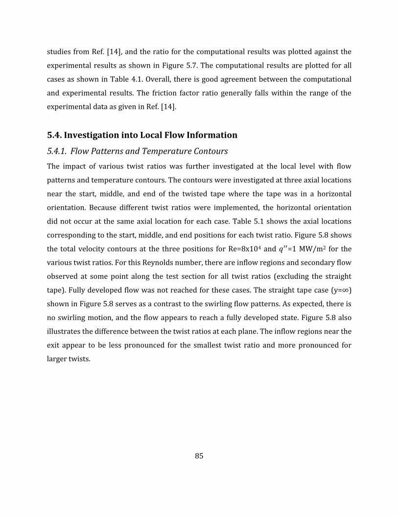
85

studies from Ref. [14], and the ratio for the computational results was plotted against the

experimental results as shown in Figure 5.7. The computational results are plotted for all

cases as shown in Table 4.1. Overall, there is good agreement between the computational

and experimental results. The friction factor ratio generally falls within the range of the

experimental data as given in Ref. [14].

5.4. Investigation into Local Flow Information

5.4.1. Flow Patterns and Temperature Contours

The impact of various twist ratios was further investigated at the local level with flow

patterns and temperature contours. The contours were investigated at three axial locations

near the start, middle, and end of the twisted tape where the tape was in a horizontal

orientation. Because different twist ratios were implemented, the horizontal orientation

did not occur at the same axial location for each case. Table 5.1 shows the axial locations

corresponding to the start, middle, and end positions for each twist ratio. Figure 5.8 shows

the total velocity contours at the three positions for Re=8x104 and 𝑞′′=1 MW/m2 for the

various twist ratios. For this Reynolds number, there are inflow regions and secondary flow

observed at some point along the test section for all twist ratios (excluding the straight

tape). Fully developed flow was not reached for these cases. The straight tape case (y=∞)

shown in Figure 5.8 serves as a contrast to the swirling flow patterns. As expected, there is

no swirling motion, and the flow appears to reach a fully developed state. Figure 5.8 also

illustrates the difference between the twist ratios at each plane. The inflow regions near the

exit appear to be less pronounced for the smallest twist ratio and more pronounced for

larger twists.

86

Figure 5.7: Ratio of the isothermal swirl flow friction factor to the axial friction factor compared to experimental data as cited in Ref. [14] [13, 14, 22, 23, 66, 67]

Table 5.1: Axial locations selected for the local flow investigation

Test Section

Location Plane

y=2 Axial

Location [m]

y=3 Axial

Location [m]

y=4.5 Axial

Location [m]

y=6 Axial

Location [m]

y=∞ Axial

Location [m]

Start 1 1.54614 1.55673 1.57262 1.58850 1.55673

Middle 2 3.07110 3.08169 3.09758 3.11346 3.08169

End 3 4.55370 4.54311 4.52723 4.51134 4.54311

87

Figure 5.8: Comparison of diabatic total velocity contours as the flow moves downstream for various twist ratios (Re=8x104, 𝑞′′=1 MW/m2)

88

The local temperature contours were also investigated at multiple axial locations and

across various twist ratios. The temperature contours were investigated at two axial

locations near the middle and end of the test section (as shown in Table 5.1). The contour is

not presented for the start of the test section because the temperature was nearly constant

at that position. Figure 5.9 shows the temperature contours for Re=8x104 and 𝑞′′=1

MW/m2 for a twist ratio of y=2. As expected, the temperature increases as the fluid moves

downstream. Similarly to the initial diabatic investigation (see Section 4.3.2), the maximum

temperature is greater than saturation (Tsat≈100°C) for this Reynolds number and heat

flux combination. This occurs near the end of the test section.

In fusion relevant geometries, the test section would be much shorter, and thus, boiling

would not be induced for this case. Furthermore, higher pressures would be implemented

at fusion relevant conditions, which would increase the saturation temperature and

suppress boiling. Figure 5.10 shows the variation in the temperature contours across

different twist ratios. Similar to the flow patterns shown in Figure 5.8, the temperature

contours vary across each twist ratio investigated.

5.4.2. Further Investigation of Inflow Regions

The secondary circulation in the twisted tape induced swirl flow results in inflow regions

which were shown to correspond to regions of low wall shear stress, low heat transfer

coefficients, and high surface temperatures in Chapter 4. The impact of the twist ratio on

this phenomenon is further investigated in this section.

The effect of the twist ratios can be qualitatively viewed by comparing the velocity and

temperature contours at a particular axial location. The velocity and temperature contours

were previously compared for a twist ratio of y=3 (see Figure 4.10). This comparison

revealed that hot spots appeared to correspond to inflow regions. The connection was

further investigated for various twist ratios in this study. Figure 5.11 shows the contours

for Re=1.5x105 and 𝑞′′=1 MW/m2 at a plane near the exit region for various twist ratios. As

shown in Figure 5.11, the connection between the inflow regions and hot spots still occurs

across various twist ratios (as indicated by arrows).

89

Figure 5.9: Comparison of temperature contours as the flow moves downstream (Re=8x104, 𝑞′′=1 MW/m2, y=2)

Figure 5.10: Comparison of temperature contours for various twist ratios at a plane near the exit region (Plane 3 in Table 5.1, Re=8x104, 𝑞′′=1 MW/m2)

90

Figure 5.11: Total velocity (top) and temperature (bottom) contours at a plane near the exit region (Plane 3 in Table 5.1, Re=1.5x105, 𝑞′′=1 MW/m2)

91

The connection between the wall shear stress and potential burn out locations was

investigated further across various twist ratios. The wall shear stress, wall heat flux, and

surface temperature were exported along the full perimeter, including the water-tape and

water-tube interfaces, at a plane near the exit region (as indicated by Table 5.1). The wall

heat flux, heat transfer coefficient, wall shear stress, and surface temperature were plotted

against the entire perimeter (including water-tube and water-tape interfaces) as shown in

Figure 5.12. The wall heat flux is shown in Figure 5.12, which reveals that the heat flux goes

to nearly zero along the water-tape interface. A similar general trend is seen across all twist

ratios with y=3 and y=4 showing greater decreases in the wall heat flux along the water-

tube interface.

Figure 5.13 shows the comparison of the HTC for different twist ratios. A negative HTC

occurs at some point along the water-tape interface for the different twist ratios. This

negative HTC is due to heat transferring from the hot water to the cool tape. There is a

stark contrast between the straight tape and the twisted tapes at the water-tape interface,

where the HTC has significant valleys for the straight case. The magnitude of the HTC varies

with the twist ratios. Aside from the straight tape, the highest magnitudes at the water-tape

interface occur with the y=3 twist ratio, while the lowest magnitudes occur with the

smallest twist ratio (y=2). The inflow regions along the outer perimeter are indicated by

dips in the HTC. As shown in Figure 5.13, the straight tape case shows no indication of

inflow regions (as expected), while the other cases show varying levels of decreased HTC

along the water-tube interface.

Figure 5.14 shows the wall shear stress along the full perimeter. There is a wide

variation for the shear stress across the various twist ratios, and the straight tape provides

a stark contrast to the twisted tapes. In the case of the straight tape, the wall shear stress

dips at the corners rather than the water-tape or water-tube interfaces, and it experiences

a gradual increase in the stress between the corner locations. For the twisted tapes, the

greatest decreases in the wall shear stress occur at the water-tape interface.

92

Figure 5.12: Wall heat flux for various twist ratios at a plane near the exit region (Plane 3 in Table 5.1, Re=1.5x105, 𝑞′′=1 MW/m2)

93

Figure 5.13: Heat transfer coefficient for various twist ratios at a plane near the exit region (Plane 3 in Table 5.1, Re=1.5x105, 𝑞′′=1 MW/m2)

94

Figure 5.14: Wall shear stress for various twist ratios at a plane near the exit region (Plane 3 in Table 5.1, Re=1.5x105, 𝑞′′=1 MW/m2)

95

Generally, the stress appears to decrease as the tape twist increases with the smallest twist

ratio (y=2) having the overall largest wall shear stress magnitude and the largest twist

ratio (y=6) showing the lowest magnitudes (although not at every point). Along the water-

tube interface, the smallest twist ratio has the smoothest curve, which is in agreement with

the flow pattern shown in Figure 5.11. Similarly, the medium ratios (y=3 and y=4.5) appear

to have more pronounced inflow regions at the water-tube interface in Figures 4.10 and

5.11. This is confirmed by Figure 5.14 where the dips in the wall shear stress are more

pronounced for those twist ratios. Lastly, the surface temperature is shown in Figure 5.15.

In general, the lowest temperatures occur at the water-tape interface, while the peak

temperatures correspond with dips in the wall shear stress and HTC for the twisted tapes.

In contrast, the straight tape case yields peak temperatures at the corners. Overall, the

smallest twist ratio (y=2) yields lower surface temperatures along the water-tube interface

and slightly higher temperatures at the water-tape interface. There is little difference

between the other twist ratios at the water-tape interface. However, at the water-tube

interface, the largest twist ratio (y=6) appears to yield mostly higher surface temperatures.

The local wall shear stress can be further visualized by plotting the contours on the

water-tube and water-tape interfaces. Figure 5.16 shows the wall shear stress contours for

all of the twist ratios investigated for Re=1.5x105 and 𝑞′′=1 MW/m2. The contours are

shown for half of the water domain in the swirling region. For easier viewing, the geometry

is cut into sections; the cut planes and locations are indicated in Table 4.7. Figure 5.16

reveals the striping that occurs in twisted tape induced swirl flow. The striping along the

water-tube interface occurs in all cases at some point in the geometry, and it is also clearly

indicated on the water-tape interface. As the flow moves downstream, the wall shear stress

appears to smooth out along the water-tube interface for the smallest and largest twist

ratios (y=2 and 6). Furthermore, the contours give an indication for the wall shear stress

magnitudes across different twist ratios. The shear stress magnitudes increase as the twist

ratio decreases. Figure 5.17 shows a portion of the straight tape case as a contrast to the

swirling flow. Note that the lowest wall shear stress occurs at the corners. This ultimately

corresponds to hot spots at the corners for the straight tape case.

96

Figure 5.15: Surface temperature for various twist ratios at a plane near the exit region (Plane 3 in Table 5.1, Re=1.5x105, 𝑞′′=1 MW/m2)

97

Figure 5.16: Wall shear stress contours for various twist ratios where cut plane locations are shown in Table 4.7 (Re=1.5x105, 𝑞′′=1 MW/m2)

98

Figure 5.17: Wall shear stress contour for the straight tape case near the exit region (Re=1.5x105, 𝑞′′=1 MW/m2)

99

5.5. Summary of Key Conclusions

The parametric study revealed a variety of results across a range of twist ratios. The key

conclusions are summarized below:

The global parameters, such as the Fanning friction factor and Nusselt number, were

shown to be in good agreement with the legacy twisted tape correlations [13-17,

22]. Likewise, Nusselt number and friction factor ratios fell within experimental

ranges when compared to legacy data [14, 17].

The friction factor decreased with increasing twist ratios. Thus, a more gradual

swirling motion resulted in a lower hydraulic resistance as opposed to a tighter

twist. Additionally, the Reynolds number and applied heat flux had a minimal

impact on the friction factor.

A better thermal performance was noted for smaller twist ratios as the Nusselt

number was shown to decrease with increasing twists. An improved performance

was also seen for higher Reynolds numbers and higher heat fluxes. Furthermore, the

Nusselt number was determined to be more sensitive to the thermal-hydraulic

parameters when compared to the friction factor.

Fully developed flow was not reached for the twist ratios investigated as the flow

continued to change downstream. Similar qualitative features were captured for

each twist ratio. However, the inflow regions near the exit appeared to be less

pronounced for the smallest twist ratio and more pronounced for the larger twists.

For the swirling flow, inflow regions were shown to correspond to regions of low

wall shear stress, low heat transfer coefficients, and high surface temperatures.

There were slight variations due to the different twist ratios. Generally, the wall

shear stress appeared to decrease as the twist ratio increased. The smallest twist

ratio had the largest overall wall shear stress magnitude, while the largest twist

yielded the lowest magnitude. This corresponded to generally lower surface

temperatures for the small twist ratio and higher temperatures for the large twist

ratio.

100

The straight tape was investigated for contrast to the swirling flow. As expected,

there were no inflow regions for this case. The decreases in wall shear stress

occurred at the corners rather than the water-tape or water-tube interfaces, which

led to peak temperatures at these locations.

Investigation of the wall shear stress contours revealed a striping pattern at some

point in the geometry for all twist ratios. As the flow moved downstream, the wall

shear stress appeared to smooth out along the water-tube interface for the smallest

and largest twist ratios.

101

Chapter 6: Computational Investigation at Fusion Relevant Conditions Portions of this work have been submitted for publication in the following peer-reviewed manuscript in which the author performed all analysis: E. Clark, A. Lumsdaine, J. Boscary, H. Greuner, and K. Ekici, "Thermal-hydraulics modeling for prototype testing of the W7-X high heat flux scraper element," Submitted to Fusion Engineering and Design, 2017.

6.1. Monoblock Plasma Facing Components Esssentially, the monoblock concept consists of armor tiles with a hole drilled through

them. A cooling tube is inserted into the hole and joined to the tiles. Monoblocks have

widespread implementation in the fusion community and are often employed in multiple

regions in magnetic confinement devices such as the divertor and the first wall. They are

planned for use in ITER, W7-X, JT60-SA, and WEST, to name a few [3, 5, 68-70]. A mock-up

of a monoblock PFC prototype intended for use in the W7-X divertor region is shown in

Figure 6.1.

The armor material varies across magnetic confinement devices, but two materials are

most prevalent in the field: carbon-carbon fiber composite (CFC) and tungsten. Tungsten is

currently the most popular armor material in magnetic confinement devices and has been

chosen for machines such as ITER and WEST [68, 70]. It is often chosen over CFC because

carbon is prone to tritium retention, which leads to radiological considerations [71, 72].

Thus, for machines that intend to run deuterium-tritium (D-T) campaigns, tungsten has

become the material of choice. However, some magnetic confinement experiments plan to

run only deuterium-deuterium (D-D) campaigns, where the issue of tritium retention is not

a factor. CFC armor is often used in these experiments and has been chosen for machines

such as W7-X and JT60-SA [3, 5].

102

Figure 6.1: Computer-aided drawing (CAD) of a W7-X monoblock plasma facing component prototype with (a) side and (b) axial viewpoints

103

In this chapter, the thermal-hydraulic parameters will be ramped up to fusion relevant

conditions from the moderate ones utilized in Chapters 4 and 5. Because this work was

generously funded by the Office of Fusion Energy Sciences for collaboration with the W7-X

project, the fusion relevant investigation will focus on conditions that align with the

interests of the W7-X experiment.

6.2. Computational Model

6.2.1. Monoblock Model Geometry

The monoblock model was developed to match W7-X prototype testing of a single

monoblock “finger” or “unit.” Boscary et al. performed experiments on a single monoblock

finger for the W7-X high heat flux scraper element [53]. As discussed in Ref. [3, 27, 53], the

so-called scraper element was created to reduce heat loads on sensitive divertor regions.

Currently, one scraper element is planned for each ten discrete divertor locations as seen in

Figure 6.2. Each scraper element is made up of 24 monoblock units and is actively cooled

with water. Previous studies were performed to determine the optimum flow configuration

for the scraper elements. It was determined that the best design consisted of parallel flow

into six different modules, which are composed of four monoblock units each [27]. The

scraper element flow sequence is illustrated in Figure 6.3.

Each of the 24 monoblock units have armor made of carbon fiber reinforced carbon

composite (CFC NB31). The CFC monoblocks are joined to a copper alloy (CuCrZr) tube by

an active metal casting (AMC®) copper interlayer, which is 0.4 mm thick. The monoblock

units have a total length of 247 mm, while the tubes are 307 mm long. The CuCrZr tubes

have an inner diameter of 12 mm and a thickness of 1.5 mm, and they are equipped with a

copper twisted tape insert. The twisted tape has a twist ratio of y=2, a tape thickness of 1

mm, and a length of 297 mm. Further specifications on the manufacturing of the monoblock

geometry can be found in Ref. [53]. Figure 6.4 shows the monoblock model geometry from

the side and axial viewpoints. The various components such as the CFC, AMC® interlayer,

pipe, and water are indicated in the axial viewpoint.

104

Figure 6.2: W7-X divertor region with scraper element [3]

Figure 6.3: Scraper element flow sequence illustration [3]

105

Figure 6.4: CFC monoblock geometry implemented in CFX

106

The prototype testing for the scraper element PFCs was performed in the Garching

Large Divertor Sample (GLADIS) high heat flux test facility at the Max Planck Institute for

Plasma Physics located in Garching, Germany [53, 73]. An initial computational

investigation into the thermal-hydraulic performance of the prototypes was performed by

this author, and the results can be seen in Figures 5 and 6 of Ref. [53]. In the initial

investigation, discrepancies were noted between the simulations and the measured data.

The discrepancies were investigated further by this author, and the work was summarized

in a recently submitted paper denoted by Ref. [74]. The investigation of the discrepancies

has been included in the dissertation for completeness and will be discussed in Section 6.6.

The computational models used in the previous studies [53, 74] were repurposed to

investigate the local flow information at fusion relevant conditions for this dissertation.

Previous monoblock studies [53, 74] were performed by this author with the SST

turbulence model because it was presumed to be superior to the other models. However,

following the investigation in Chapter 4, the turbulence model was changed to k-epsilon to

maintain consistency with Chapters 4 and 5 of this dissertation.

6.2.2. Fusion Relevant Conditions

The conditions for the model setup were chosen to match the experimental parameters

investigated in Ref. [53]. The GLADIS test facility is equipped with two sources, which

impose a Gaussian loading distribution [73]. The prototypes were placed normal to the

beam, and they were cooled with water at a velocity of 12 m/s (including the increased

speed due to the twisted tape). The static pressure was 1 MPa, and three peak heat fluxes

(PHFs) were investigated: 10.5, 15, and 20 MW/m2 [53].

In the computational setup, a uniform inlet axial velocity was applied for the water at

10.727 m/s. Including the increased velocity due to the twisted tape, this leads to a

velocity of 12 m/s. For comparison to the studies in Chapters 4 and 5, the inlet Reynolds

number was 1.25x105. The inlet temperature and exit pressure were set to 20°C and 1 MPa,

respectively. A Gaussian heat flux profile was applied at the three peak heat fluxes (10.5,

15, and 20 MW/m2). The surface heat flux distribution for the 10.5 MW/m2 case is shown

107

in Figure 6.5. Note that the peak heat flux is not centered on the CFC monoblock. Instead,

the peak is specified to occur at 0.1615 m down the length of the CFC. This specification

was made in accordance with the prototype testing [53, 75].

Conjugate heat transfer was modeled from the CFC surface through the solid regions

(including the AMC® interlayer and CuCrZr tube) and into the water. Heat transfer was

also modeled throughout the solids and the water along with the water-tape interfaces.

There was no gap included between the tape and the tube. Instead, the tape-tube interfaces

were considered to be adiabatic so that fin effects were not captured in this model.

Furthermore, radiation effects were considered to be negligible and were not considered

for this work.

Temperature and pressure dependent water properties were implemented with the

IAPWS IF-97 formulation [54]. Orthotropic and temperature dependent thermal

conductivity values were implemented for the CFC according to equations given in Ref. [76-

78]. Figure 6.6 shows the temperature dependent thermal conductivity used for the CFC

material. The rest of the solid materials were implemented with constant properties as

shown in Table 6.1 [75, 79, 80]. The prototype tests were completed with a copper twisted

tape, but the simulations were performed with a stainless steel (SS316) tape. However, this

should not have an impact on the solution because the heat transferred to the tape does not

make up a significant portion of the heat exchanged in the system.

Simulations for the three PHFs were performed with the k-epsilon turbulence model. A

mesh study was performed for the 20 MW/m2 case, and the mesh was refined successively

until the maximum temperature in the solids, the average water temperature at the outlet,

and the pressure drop changed less than 1% from case to case. The meshing criterion was

chosen such that an average volume non-dimensional wall coordinate of y+≈>30 was

generated for the highest PHF. The mesh refinement was performed only for the highest

PHF because it would result in the most extreme temperatures. Lower temperatures, and

thus lower non-dimensional wall coordinates, would be expected for lower PHFs. The same

mesh was used for all peak heat fluxes investigated.

108

Figure 6.5: Gaussian heat flux profile applied to a monoblock finger [74]

Figure 6.6: Temperature dependent thermal conductivity of CFC NB31 [74]

109

Table 6.1: Material properties implemented for solid components [75-80]

Material Density [kg/m3]

Specific Heat Capacity [J/kgK]

Thermal Conductivity [W/mK]

AMC® Copper [75, 79] 8933 385 150

CuCrZr [80] 8900 390 326

SS316 [80] 8031 465 14 CFC NB31 [76-78] 1959 1031 See Figure 6.6

110

The mesh for this study is shown in Figure 6.7. Inflation layers were implemented on the

water-tube and water-tape interfaces. The tube element sizing was chosen to match the

water sizing for an acceptable mesh aspect ratio at the water-tube interface. The AMC®

interlayer sizing was chosen such that the thickness was resolved by at least two elements,

and the CFC sizing was selected to match the element sizing on the tube. The volume-

averaged non-dimensional wall coordinate for the water was y+≈29, 32, and 35 for a PHF of

10.5, 15, and 20 MW/m2, respectively.

6.2.3. Post-Processing Method

As shown in Figure 6.8, the experimental data from the prototype testing was taken from

infrared images of the CFC surface at the location of PHF. The data was taken at three

points: the monoblock center and two edge locations. For comparison to the experiments,

three points were created at the same locations along the CFC surface as shown in Figure

6.9. Data was pulled from these locations in the post-processor and will be compared to the

experimental results in Section 6.3.

Furthermore, circumferential distributions were investigated at various axial locations.

These distributions were created in a similar fashion to those discussed in Chapters 4 and

5. The data was extracted along the water-tube interface at a plane of interest. However,

the calculation of the angular coordinate was slightly more complicated due to the

monoblock geometry and the origin location. Figure 6.10 shows the angular coordinate on

the monoblock geometry along with the origin and center point location. The angle (θ) was

calculated based on the x- and z-coordinates by factoring in the offset from origin.

111

Figure 6.7: Axial and close-up side view of the implemented mesh for the CFC monoblock geometry

112

Figure 6.8: Infrared image of the monoblock prototype at PHF of 20 MW/m2 as seen in Ref. [53]

Figure 6.9: Points for post-processing simulations [74]

113

Figure 6.10: Angular coordinate for monoblock geometry circumferential distributions

114

6.3. Comparison to Prototype Testing

6.3.1. Initial Comparison

The computational results were compared to the experimental data collected from the

GLADIS high heat flux testing as seen in Ref. [53]. Figures 6.11 and 6.12 show the

comparisons at the center and edges of the monoblock, respectively. In the experiments, a

discrepancy was revealed between the temperature values at the two edges. Thus, Ref. [53]

provides the results for both edge locations. However, there was no notable asymmetry at

the edges in the simulations. The computational results shown in Figure 6.12 were taken at

the Edge 1 location as shown in Figure 6.9. Such discrepancies between the simulations and

the measurements will be further discussed in Section 6.6.

As seen in Figure 6.11, the computational results are lower than the experimental data

at PHF of 10.5 and 15 MW/m2. However, at a PHF of 20 MW/m2, the simulations fall within

the experimental range. The computational results are closer to the experiments at the

edges. Figure 6.12 reveals that the simulations yield results that are near the bottom range

of the experimental data for a PHF of 10.5 MW/m2, and they fall within the experimental

range at a PHF of 15 MW/m2. Note that the experimental data at a PHF of 20 MW/m2 along

the edges was thrown out by the authors; further insight into this decision can be found in

Ref. [53].

6.3.2. Further Investigation of Results

Aside from the comparison to the experimental data, the thermal performance was

investigated further by viewing the temperature contours for various computational

domains. Figure 6.13 shows the temperature contours for the computational domains of

interest such as the CFC, AMC® copper interlayer, CuCrZr tube, and the water for a PHF of

10.5 MW/m2. The twisted tape was not included because only a limited amount of heat was

transferred between the water and the tape.

115

Figure 6.11: Comparison of experimental [53] and CFX results at the center of the monoblock

Figure 6.12: Comparison of experimental [53] and CFX results at the edges of the monoblock

116

Figure 6.13: Temperature contours of computational domains including the (a) CFC, (b) AMC® copper interlayer, (c) CuCrZr tube, and (d) water for a PHF of 10.5 MW/m2

117

It should be noted that, even for the lowest PHF case, the temperatures are still extreme.

At 1 MPa, the saturation temperature is Tsat≈180°C, and as seen in Figure 6.13, the water

temperature is greater than saturation underneath the region of PHF. The peak

temperature values for each computational domain of interest are shown in Table 6.2. In

each case, the peak water temperature is greater than saturation. This indicates that one

would expect to see boiling for these cases. Furthermore, the temperature values in the CFC

are extreme. According to Ref. [3], the design limits for the W7-X scraper element require

the CFC surface temperature to be below 1200°C. In the cases of 15 and 20 MW/m2 PHF,

the peak CFC temperature exceeds this design criterion.

Figure 6.13 also highlights the variation of the temperature distributions due to a one-

sided Gaussian heat flux application. The circumferential temperature distribution was

created under the location of PHF using the post-processing method discussed in Section

6.2.3. The temperature distribution around the water-tube interface is shown in Figure

6.14. Again, in all cases the water temperature exceeds the saturation temperature.

Because of the one-sided heat flux application, the upper surface of the water-tube

interface is hotter than the lower side. Furthermore, this distribution indicates that

subcooled boiling would be expected to occur on the top surface while convection would

occur on the bottom surface.

These results qualitatively agree with those found in the literature. Boscary et al.

performed an investigation of the critical heat flux of subcooled water in twisted tape

enabled tubes under one-sided heating. As part of their study, the authors performed a

finite element investigation of the temperature distribution in the monoblock armor and at

the water-tube interface. For the water-tube interface, they concluded that the subcooled

boiling regime occurred at the upper portion whereas the convection was dominant in the

lower portion of the water [64]. Figure 6.15 shows the comparison between the monoblock

armor temperature distributions for the current study and Ref. [64]. The distribution for

the current study is shown at the location of PHF for 10.5 MW/m2. As seen in Figure 6.15,

the results are qualitatively similar. The isotherms show a similar pattern throughout the

monoblock.

118

Table 6.2: Peak temperature values in domains of interest for all PHF

Domain Peak Temperature [°C]

PHF=10.5 [MW/m2]

PHF=15 [MW/m2]

PHF=20 [MW/m2]

CFC Armor 901 1457 2094 AMC® Copper

Interlayer 331 445 570

CuCrZr Tube 291 388 492

Water 233 301 374

Figure 6.14: Circumferential temperature distributions for various PHF on the monoblock geometry

119

Figure 6.15: Monoblock temperature distributions for (a) Ref. [64] and (b) the current study at the location of PHF for 10.5 MW/m2

120

Lastly, the expected boiling regions were investigated in the post-processor. Regions

where the water temperature was greater than saturation are shown for each PHF

investigated in Figure 6.16. The expected boiling regions cover a notable portion of the

water domain, especially for the PHF of 15 and 20 MW/m2. The assumptions and governing

parameters of the single-phase model begin to break down as the water temperature

approaches and surpasses the saturation temperature. These results highlight the need for

the inclusion of the second phase in fusion relevant simulations. Inclusion of the boiling

process would result in overall lower temperatures because the phase change would create

increased heat transfer at the water-tube interface. This would actually increase the gap

between the computational results and the experimental data gathered from the prototype

testing in Ref. [53].

It should be noted that higher pressures could be used in fusion relevant experiments,

which could mitigate some of the boiling due to increased saturation temperatures. For

example, recent ITER experiments have cited pressure values as high as 4 MPa where the

saturation temperature is Tsat≈250°C [70]. At that pressure, the water temperature

distribution would remain below saturation for a PHF of 10.5 MW/m2. However, as seen in

Clark et al. [3], the W7-X divertor scraper element is design to handle pressures up to about

2.5 MPa where the saturation temperature is Tsat≈224°C. In this case, the peak water

temperatures seen in this study are still greater than saturation for all PHF investigated.

6.4. Analysis of Local Flow Information In Chapters 4 and 5, local flow information was investigated for a general geometry at

moderate, uniform heating conditions. The investigation revealed that the secondary

circulation resulted in so-called “inflow regions” where the boundary layer fluid was

reinjected into the freestream. These inflow regions were shown to correspond to regions

of low wall shear, low heat transfer coefficients, and high surface temperatures. Thus,

inflow regions were proposed as likely candidates for early burnout in twisted tape

devices.

121

Figure 6.16: Expected boiling regions for PHF of (a) 10.5 MW/m2, (b) 15 MW/m2, and (c) 20 MW/m2

122

Furthermore, examination of the wall shear stress exposed an apparent “striping” that

developed in the twisted tape induced swirl flow. The so-called stripes represent the inflow

regions along the water-tube interface; the number and location of the stripes shifts along

the test section.

To this author’s knowledge, the connection between the inflow regions to possible

burnout locations and the wall shear stress striping has not been identified in the twisted

tape induced swirl flow literature. In this chapter, a similar investigation into the local flow

information will be performed at fusion relevant conditions. The main objectives will be to

investigate if the inflow regions and wall shear stress striping still occur at fusion relevant

conditions. Furthermore, the connection between the wall shear stress, heat transfer

coefficient, and surface temperature will be examined to see if these relationships between

these variables still have a significant impact at fusion relevant heating values.

6.4.1. Flow Patterns and Temperature Contours

The flow patterns and temperature contours were investigated for the monoblock

geometry at fusion relevant conditions. Figure 6.17 (a) shows the total velocity contour for

a PHF of 10.5 MW/m2, while Figure 6.17 (b) shows the tangential velocity vectors at a

plane near the exit. The results are qualitatively similar to those seen in Chapter 4 at the

moderate heating conditions and in the adiabatic flow visualization experiments [22, 23].

Inflow regions still occur in this case near the exit region, where the secondary flow causes

a thickening of the boundary layer (as denoted by arrows).

The flow patterns were investigated at various axial locations for all fusion relevant

cases (as provided in Table 6.3). Note that the origin is located at the bottom left corner of

the monoblock armor in the model geometry. The locations were chosen such that the tape

was in a horizontal orientation near the beginning, middle, and end of the test section.

Figure 6.18 shows the total velocity contours at three axial locations for a PHF of 10.5

MW/m2. The hydraulic solution was the same for each PHF investigated.

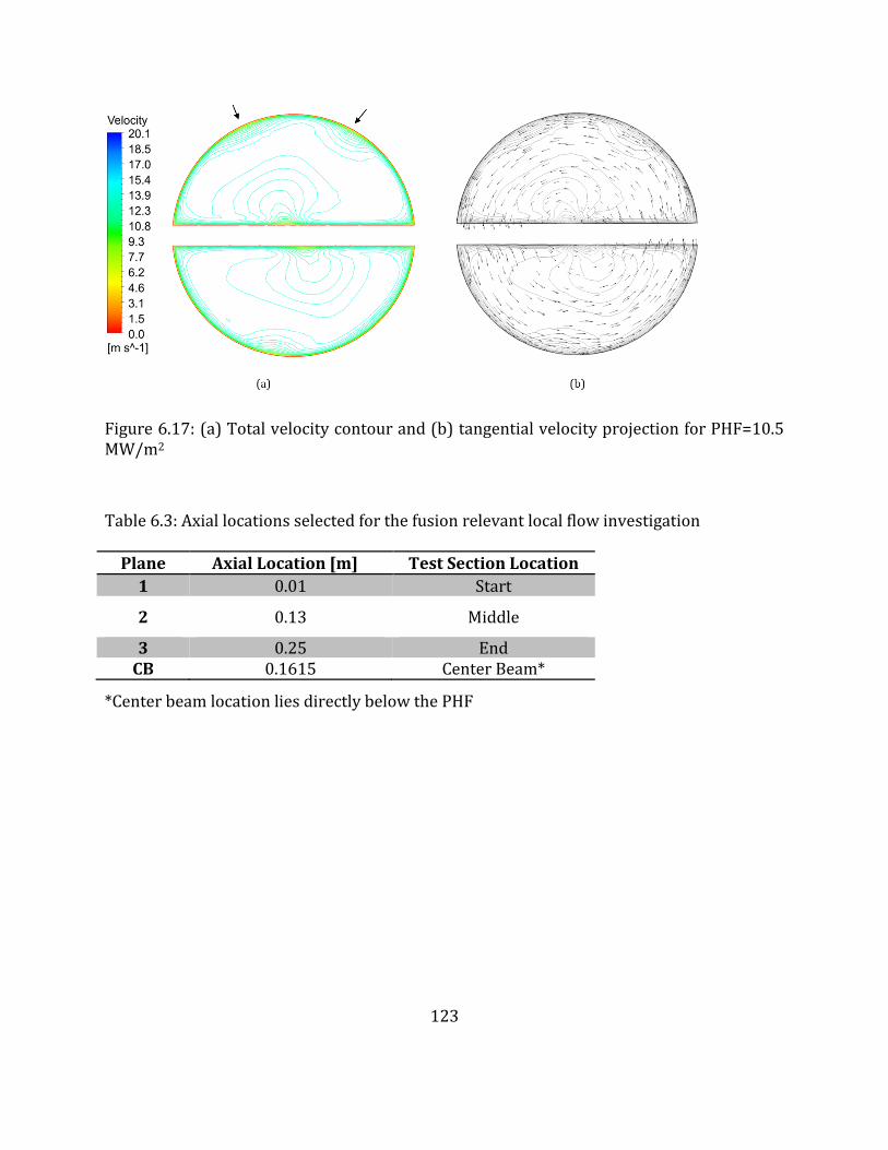
123

Figure 6.17: (a) Total velocity contour and (b) tangential velocity projection for PHF=10.5 MW/m2

Table 6.3: Axial locations selected for the fusion relevant local flow investigation

Plane Axial Location [m] Test Section Location

1 0.01 Start

2 0.13 Middle

3 0.25 End CB 0.1615 Center Beam*

*Center beam location lies directly below the PHF

124

Figure 6.18: Comparison of total velocity contours as the flow moves downstream for the monoblock geometry (PHF=10.5 MW/m2)

Fully developed flow was not noted in the monoblock geometry. This is not surprising due

to the short tube geometry included in the model. As seen in Figure 6.18, the secondary

flow appears to be developing near the beginning (Plane 1), and inflow regions can be seen

near the middle and exit locations.

The local temperature contours were also investigated at two axial locations for the PHF

of 10.5 MW/m2. Figure 6.19 shows the comparison between the total velocity contours and

the temperature contours for two axial locations: under the PHF location and near the exit.

In both locations, the inflow regions appear to have a qualitative connection to the local

temperature contour (as indicated by the arrows). However, under the location of PHF (at

Plane CB), there is an extreme temperature gradient in the flow field. This large gradient

makes it difficult to glean information from the contour. The water-tube interface values

will provide a better insight into the possible connection between inflow regions and the

surface temperature. Figure 6.19 also reveals the large temperature difference between the

two axial locations. The maximum temperature at the location of PHF is over five times

higher than the peak temperature near the exit region.

125

Figure 6.19: Comparison of total velocity and temperature contours under the location of PHF (Plane CB) and near the exit (Plane 3) for the monoblock geometry (PHF=10.5 MW/m2)

126

6.4.2. Further Investigation of Inflow Regions

As discussed in Chapter 4, the secondary flow causes thickening of the boundary layer at

the inflow regions, and this local boundary layer thickening was shown to result in a lower

wall shear stress, which corresponded to a lower heat transfer coefficient and thus, a

higher surface temperature in those regions. Furthermore, the inflow regions were shown

to correspond to an apparent “striping” of low wall shear stress when viewing the full

contours. These relationships will be investigated further in this section to determine if

they are still prevalent at fusion relevant conditions.

The wall shear stress can be visualized by viewing the contours along the water-tube

interfaces. Figure 6.20 shows the wall shear stress contours for all of the PHF investigated

for the monoblock geometry. As seen in Figure 6.20, the shear stress contours reveal a

striping pattern, which suggests that this phenomenon is still prevalent at fusion relevant

conditions.

The wall shear stress, wall heat flux, and surface temperature were exported along the

perimeter for two axial locations: under the PHF and near the exit. The heat transfer

coefficient (HTC) was calculated at each surface point using Eq. 4.6 along with the mean

temperature as shown by Eq. 4.7. Due to the different tape orientations, the results were

compared along the water-tube interface. All the data was extracted for a PHF of 10.5

MW/m2 and was plotted against the angular coordinate as shown in Figure 6.10.

The wall shear stress and wall heat flux at the location of PHF are shown together in

Figure 6.21. Similarly, the wall shear stress and HTC are shown together in Figure 6.22, and

the wall shear stress and surface temperature (Ts) are shown in Figure 6.23. Figure 6.21

reveals the connection between the wall shear stress and the wall heat flux, which is

similar to the uniform heating results seen in Chapter 4. There does appear to be a

connection between the wall shear stress and the wall heat flux. However, it does not

appear to be as strong as the connection viewed in Chapter 4. Locations of low wall shear

correspond to slight decreases or flattening of the curve.

127

Figure 6.20: Wall shear stress contours for the monoblock geometry

128

Figure 6.21: Comparison of wall shear stress and wall heat flux along the water-tube interface at the location of PHF (Plane CB in Table 6.3, PHF=10.5 MW/m2)

Figure 6.22: Comparison of wall shear stress and HTC along the water-tube interface at the location of PHF (Plane CB in Table 6.3, PHF=10.5 MW/m2)

129

Figure 6.23: Comparison of wall shear stress and surface temperature along the water-tube interface at the location of PHF (Plane CB in Table 6.3, PHF=10.5 MW/m2)

130

The connection between the wall shear stress and the HTC is shown in Figure 6.22. The

relationship is more pronounced here where dips in the wall shear stress result in clear

dips in the HTC. Conversely, the connection between the wall shear stress and the surface

temperature is not apparent in this case as can be seen in Figure 6.23. The dips in the wall

shear stress no longer noticeably correspond to peaks in the surface temperature. As

discussed in Section 6.3.2, the general trend of the surface temperature is as expected in

the literature [64]. However, locally, it does not appear to be affected by the wall shear

stress. This is further illustrated by a zoomed in view of the peak surface temperature as

shown in Figure 6.24.

Figure 6.25 shows the comparison between the wall shear stress and the surface

temperature at a plane near the exit region. A similar behavior was observed, where the

temperature gradient is much lower than the location of PHF. Even with the moderate

gradient seen in Figure 6.25, the wall shear stress did not appear to have a great impact on

the surface temperature.

6.5. Discussion of Local Relationships at Fusion Relevant Conditions The lack of a prevalent connection between the surface temperature and wall shear stress

results at fusion relevant conditions necessitated further investigation into the

relationship. A few items were explored including the global effect on full contours, IAPWS

water properties, near wall behavior, and the connection at lower peak heat fluxes.

6.5.1. Full Contour Comparison

The full monoblock contours were viewed to investigate the relationship between the wall

shear stress, wall heat flux, and temperature. Figure 6.26 shows the comparison between

the three variables for the whole water domain from a top down viewpoint. From this

perspective, the wall shear striping appears to have a noticeable effect on the wall heat flux

(as indicated by the arrows). However, there looks to be a very small effect on the

temperature.

131

Figure 6.24: Close-up view of the peak surface temperature along the water-tube interface at the location of PHF (Plane CB in Table 6.3, PHF=10.5 MW/m2)

Figure 6.25: Comparison of wall shear stress and surface temperature along the water-tube interface near the exit region (Plane 3 in Table 6.3, PHF=10.5 MW/m2)

132

Figure 6.26: Comparison of wall shear stress, wall heat flux, and surface temperature for the full water domain from the monoblock geometry (Top down viewpoint)

133

6.5.2. Investigation of IAPWS Water Properties

As discussed in Section 6.3, the peak temperatures from the computational solutions were

greater than the saturation temperature. However, the computational model is constricted

to single-phase, which could potentially lead to unrealistic property values from the IAPWS

library. The phase diagram for the IAPWS equations implemented in ANSYS CFX is shown

in Figure 6.27 where the numbered regimes represent the following phases [42, 54]:

1. Subcooled water

2. Supercritical water/steam

3. Superheated steam

4. Saturation data

5. High temperature steam

Regimes 1-4 are included in CFX, and this author’s calculations were performed with

IAPWS equations from Regime 1 only. The peak water temperatures are shown again in

Table 6.4. Comparison between the phase change diagram and the peak water

temperatures reveals that PHF of 10.5 and 15 MW/m2 fall within the temperature and

pressure ranges of Regime 1. However, the temperature exceeds the subcooled water

regime for a PHF of 20 MW/m2 by roughly 25°C. With a pressure of ≈1 MPa, this places the

PHF of 20 MW/m2 in Regime 4.

The behavior of the water properties was investigated for the subcooled water regime.

Figure 6.28 shows the density (ρ), specific heat capacity (cp), dynamic viscosity (μ), and

thermal conductivity (k) over a range of temperatures at 1 MPa. These figures reveal sharp

changes in the water properties at approximately 320°C. Thus, the fusion relevant

investigation is stretching the limits of the single-phase model and the IAPWS properties

implemented in it.

134

Figure 6.27: Water property regimes for the IAPWS IF-97 formulation as implemented in ANSYS CFX [42, 54]

Table 6.4: Peak water temperature for the monoblock model

PHF Peak Water

Temperature [K]

10.5 506

15 575

20 647

135

Figure 6.28: IAPWS water properties in the subcooled water regime

136

6.5.3. Investigation of Near Wall Behavior

The near wall behavior was investigated for a PHF of 10 MW/m2 at three axial locations

including Plane 2, Plane 3 and Plane CB as seen in Table 6.3. The velocity and temperature

profiles were investigated near the wall at the top of the tube—where the heat flux is

applied. For this analysis, a line was created near the wall from two points as shown in red

in Figure 6.29, and fifteen points were sampled along the line (Note: there are only nine

mesh points along this line). The total velocity and temperature profiles were plotted

against the distance from the wall as shown in Figures 6.30 and 6.31. Figure 6.31 reveals

extreme temperature gradients at locations where significant heat is applied (Plane 2 and

Plane CB). However, large temperature gradients are to be expected for twisted tape

devices. As discussed by Manglik and Bergles, passive heat transfer enhancement

techniques tend to generate “well-mixed” flows with considerably sharper wall

temperature gradients than normal [8]. Such large temperature gradients could be used as

justification for the use of a low Reynolds number approach for the turbulence modeling

where the model has the capability to resolve the flow near the wall (such as SST or

Reynolds stress models).

Figure 6.29: Sampling line utilized in near wall investigation

137

Figure 6.30: Total velocity profiles in the near wall region at three axial locations as given in Table 6.3

138

Figure 6.31: Temperature profiles in the near wall region at three axial locations as given in Table 6.3

139

The non-dimensional velocity and temperature profiles were also determined as part of

the near wall investigation. The profiles were created following the guidance of Ref. [39] as

discussed in Chapter 3. The water properties and the axial velocity were exported along the

line shown in Figure 6.29. Points were created at the top of the line at the water-tube

interface for the variables at the wall. The dimensionless velocity (u+) was calculated from

Eq. 3.8 and 3.10, while the dimensionless temperature (T+) was determined from Eq. 3.15

and 3.16. The non-dimensional velocity and temperature were plotted against the

dimensionless wall coordinate (y+) as given by Eq. 3.9.

The dimensionless velocity and temperature profiles are shown in Figures 6.32 and

6.33, respectively. These profiles reveal that the first node away from the wall has a non-

dimensional wall distance in the range of y+≈50-60. The location of peak heat flux (Plane

CB) has a higher y+ due to the increased temperature in that region.

The near wall behavior was discussed in detail in Chapter 3. Review of this discussion

suggests that a dimensionless wall distance of y+≈50 places the first mesh point outside of

the buffer region in the log law or overlap layer. This falls in line with the assumptions of

the wall function approach, which was utilized due to the implementation of the k-eps

model for these simulations. The use of wall functions prevents a full resolution of the near

wall behavior, and thus, the viscous sublayer and buffer layer are not represented in

Figures 6.32 and 6.33. For a full resolution of the boundary layer, a low Re approach with

an appropriately refined mesh should be implemented. While the viscous sublayer and

buffer layer are not shown here, the data reveals similar behavior to the velocity profiles

shown in Ref. [39, 44]. The overlap layer is represented by the linear portion of the curve,

and the defect layer is represented by curved portion. For example, consider Plane 3 in

Figure 6.32. The overlap or log law region is represented by the linear trend from y+≈50-

110. The defect layer follows at y+>110. While not as distinct, this transition can be seen at

the other planes as well. The transition is not as clear in the dimensionless temperature

profile for Planes 2 and CB because of the higher temperature gradients at those planes.

140

Figure 6.32: Non-dimensional velocity profile in the near wall region

141

Figure 6.33: Non-dimensional temperature profile in the near wall region

142

As discussed in Chapter 3, the inner layer connects with the log law region at a

dimensionless wall coordinate of y+≈30. This inspired the selection of the mesh criteria for

this study, which included an average volume y+ of approximately 30 (as seen in Section

6.2.2). Figures 6.32 and 6.33 reveal the local variation in the y+ at different locations. This

difference is especially clear at regions of higher temperatures where there are higher y+

values. In retrospect, this local variation could have been taken into account for the

meshing strategy. One could envision a more refined mesh overall where the criteria was a

dimensionless wall distance of y+≈30 at the location of peak heat flux.

6.5.4. Analysis of Local Flow Information at Lower Peak Heat Fluxes

Solutions were completed with lower peak heat fluxes to determine if the connection

between the wall shear stress and the surface temperature was more prevalent at less

extreme conditions. The model setup and conditions discussed in Section 6.2 were utilized

in these solutions. The only change was the applied peak heat fluxes, which were reduced

to 1 and 5 MW/m2.

The water temperature contours for these solutions are shown in Figure 6.34. Neither

solution reaches the saturation temperature of Tsat≈180°C. The wall shear stress, wall heat

flux, and surface temperature were exported along the perimeter at the location of PHF.

The HTC was calculated using Eq. 4.6 along with the mean temperature as given by Eq. 4.7.

The data was extracted for the lowest PHF of 1 MW/m2 and was plotted against the angular

coordinate as shown in Figure 6.10.

The wall shear stress and wall heat flux are shown together in Figure 6.35. Similarly, the

wall shear stress is compared to the HTC and the Ts in Figures 6.36 and 6.37, respectively.

Figure 6.35 reveals similar results to those seen in Section 6.3. There is an apparent

connection between the wall shear stress and the wall heat flux. Locations of low wall shear

stress correspond to slight decreases or flattening of the curve. Again, the relationship

between the wall shear stress and the HTC is more pronounced as seen in Figure 6.36.

However, as can be seen in Figure 6.37, the connection between the shear stress and the

surface temperature is still not apparent—even at much lower applied heat fluxes.

143

Figure 6.34: Water temperature contours for lower applied PHF of (a) 1 MW/m2 and (b) 5 MW/m2

Figure 6.35: Comparison of wall shear stress and wall heat flux along the water-tube interface at the location of PHF (Plane CB in Table 6.3, PHF=1 MW/m2)

144

Figure 6.36: Comparison of wall shear stress and HTC along the water-tube interface at the location of PHF (Plane CB in Table 6.3, PHF=1 MW/m2)

Figure 6.37: Comparison of wall shear stress and surface temperature along the water-tube interface at the location of PHF (Plane CB in Table 6.3, PHF=1 MW/m2)

145

This suggests that the effect of the wall shear stress striping on the surface temperature is

minimal for one-sided non-uniform heating conditions. The change in temperature due to

the depressed wall shear stress is minimal compared to the change in temperature due to

the applied heat flux. Consideration of the results seen in Chapters 4 and 5 would suggest

that this phenomenon is more important for uniform, moderate heating applications.

6.6. Investigation of Discrepancies from CFC Prototype Testing As discussed in Section 6.3.1, comparison of computational and experimental results from

the prototype testing revealed discrepancies between the simulations and measurements.

The discrepancies were investigated further by this author, and the work was summarized

in a recently submitted paper denoted by Ref. [74]. The investigation of the discrepancies

has been included in the dissertation for completeness and will be discussed in this section.

Potential explanations for the differences between the simulations and measurements

could lie in the manufacturing process of the monoblock prototypes. One uncertainty is in

the circumferential casting process, which could result in a better thermal connection at

the top and bottom as opposed to the sides of the tube. Another source of the discrepancy

could be a slight misalignment of CFC fibers in the off-normal direction. The orthotropic

CFC thermal properties depend on the orientation of the fibers, where the direction of peak

thermal conductivity is generally aligned parallel with the direction of the applied heat flux

(often the normal direction) [74, 76-78]. Slight misalignment of the fibers during

manufacturing would result in an offset in the thermal properties, and the direction of peak

thermal conductivity would align to a direction slightly off-normal [74]. While not

investigated here, it should be noted that a few other explanations have been raised to

resolve the discrepancies such as potential degradation of the CFC properties due to high

heat loads or possible property variation in different CFC batches due to the manufacturing

process. Future work could include investigations into these topics.

Parametric studies were performed to investigate the effects of a non-uniform thermal

contact resistance and misaligned CFC fibers in the monoblock geometry. The model setup,

conditions, and post-processing were utilized from Section 6.2 for these studies with one

146

exception. The turbulence model utilized in this study was the SST model, which differs

from the model utilized in the preceding chapters. Previous monoblock studies [53, 74]

were performed by this author with the SST turbulence model because it was presumed to

be superior to the other models. The results shown in Chapters 4 and 5 of this work suggest

that the turbulence models yield different global values, but they capture the same general

features in the flow field. In this section, the global values are not the focus, but rather the

effect of the different manufacturing features on the solution. Thus, it was determined that

the same behaviors could be viewed in these solutions regardless of the turbulence model

implemented.

The use of the SST turbulence model for this work necessitated a different mesh than the

one highlighted in Figure 6.7. The SST model requires a refined mesh with a suggested non-

dimensional wall coordinate of y+<1. A similar approach was taken to refine the mesh as

discussed in Section 6.2.2. A mesh study was performed for the highest peak heat flux (20

MW/m2), and the mesh was refined successively until the maximum temperature in the

solids, the average water temperature at the outlet, and the pressure drop changed less

than 1% from case to case. The same mesh was used for all peak heat fluxes investigated.

The meshing criterion was chosen such that an average volume non-dimensional wall

coordinate of y+≈<1 was generated for the highest PHF. This required the use of a smaller

first wall height and a more refined overall mesh on the solid portions than was shown in

Figure 6.7, which resulted in a larger mesh and higher computational runtimes.

6.6.1. Investigation of Non-Uniform Thermal Contact Resistance

Two parametric studies were completed to study the effect of a non-uniform thermal

contact resistance (TCR) between the CFC and the AMC® interlayer. The first was a

“baseline” case in which a constant TCR was implemented. A circumferentially varying TCR

was created for the second case in order to simulate the potential variation that could

occur as a result of the circumferential bonding process. Equation 6.1 was created for the

contact conductance (cc) on the armor-interlayer interface; the cc was set to vary from

147

1x104 to 1.5x106 W/m2K from the sides to the top and bottom of the tube, respectively

[74].

𝑐𝑐 = 7.45 × 105 cos(2𝜃 − 𝜋) + 7.55 × 105 (6.1)

The angular coordinate in Eq. 6.1 is shown in Figure 6.10. The TCR was entered into ANSYS

CFX as the inverse of the cc. The applied TCR is presented in Figure 6.38, where the

resistance is higher at the sides compared to the rest of the tube.

The computational results from the parametric studies were compared to the prototype

experimental data as discussed in Section 6.3.1 and Ref. [53]. Figures 6.39 and 6.40 show

the comparisons at the center and edges of the monoblock, respectively. Because the

computational solutions revealed no notable asymmetry at the edge, the results shown in

Figure 6.40 were taken at the Edge 1 location as shown in Figure 6.9. Similarly to Section

6.3.1, the computational results at the center of the monoblock are lower than the

experimental data at PHF of 10.5 and 15 MW/m2. However, at a PHF of 20 MW/m2, the

simulations yield results near the bottom of the experimental range. The results are once

again closer to the experiments at the edge locations as seen in Figure 6.40. The

simulations are near the bottom range of the experimental data for a PHF of 10.5 MW/m2,

and they fall within the range of experimental data at a PHF of 15 MW/m2. Note that the

experimental data at a PHF of 20 MW/m2 along the edges was thrown out by the authors;

further insight into this decision can be found in Ref. [53].

The circumferential temperature distributions for the two TCR cases are shown in

Figure 6.41. These distributions highlight the difference between a uniform and non-

uniform TCR. Note that the temperature remains below saturation for a PHF of 10.5

MW/m2 in these studies, which is in contrast to the results seen in Figure 6.14. The lower

temperatures seen in Figure 6.41 are due to the implementation of the SST turbulence for

these particular solutions.

148

Figure 6.38: Implemented non-uniform TCR on the armor-interlayer interface [74]

Figure 6.39: Comparison of experimental [53] and CFX results at the center of the monoblock for a parametric investigation of the TCR [74]

149

Figure 6.40: Comparison of experimental [53] and CFX results at the edges of the monoblock for a parametric investigation of the TCR [74]

Figure 6.41: Circumferential temperature distributions at the location of peak heat flux for a parametric investigation of the TCR [74]

150

As shown in Chapter 4, the SST model yielded higher Nusselt number values and lower

temperatures when compared to the k-eps model (which was used to generate Figure

6.14). Generally, there appears to be a minimal effect due to the circumferentially varying

TCR. As expected, the sides of the tube show the largest difference in the temperature

distribution where the TCR was higher, but there looks to be a limited effect along the rest

of the circumference.

6.6.2. Investigation of CFC Fiber Misalignment

The data from the prototype experiments revealed a notable difference between the

surface temperature at the two edge locations [53], which was not noted in the

computational results. One explanation behind this temperature difference could be the

misaligned fibers in the CFC. A minor misalignment of the fibers during the manufacturing

process could lead to misaligned thermal properties.

The CFC thermal conductivity was implemented as orthotropic and temperature

dependent according to Ref. [76-78]. To simulate a potential misalignment of CFC fibers,

the thermal properties were defined based on a rotated coordinate frame in CFX as shown

in Figure 6.42. The study was performed for a PHF of 10.5 MW/m2 and a non-uniform TCR

as shown in Figure 6.38. The coordinate frame for the thermal properties was rotated by

three angles (φ=1.7, 3, and 8.5°) to create a new reference frame (𝑦′, 𝑥′). In these cases, the

peak thermal conductivity was no longer acting in the normal direction (-𝑥), but instead

was imposed φ° off normal.

The rotated CFC properties yielded asymmetries in the surface temperature similar to

those seen in the experiments. Figure 6.43 shows the surface temperature contour for the

largest rotation angle investigated. A comparison between the edge temperature difference

(ΔTedges) from the experiments [53] and the simulations is presented in Figure 6.44.

151

Figure 6.42: Rotated coordinate frame for CFC thermal properties in investigation of fiber misalignment [74]

Figure 6.43: Surface temperature for rotated CFC fibers (φ=8.5°) with a PHF of 10.5 MW/m2 [74]

152

Figure 6.44: Comparison of edge temperature differences (ΔTedges) between experimental [53] and computational results at various CFC fiber rotation angles [74]

The average ΔTedges for a PHF of 10.5 MW/m2 was roughly 112°C in the experimental

setting. The ΔTedges yielded in the simulations is plotted directly against this average value

from the experiments. Figure 6.44 shows that a rotation of φ=3° gives an edge temperature

difference similar to the average value noted in the experiments. This reveals that even

small angles of fiber misalignment can result in asymmetries at the outer monoblock edges.

6.7. Summary of Key Conclusions The computational investigation with the monoblock geometry yielded a range of results

for the fusion relevant conditions. The key conclusions from this chapter are summarized

below:

Computational results were compared to prototype testing performed in the

GLADIS high heat flux test facility [53]. Discrepancies were noted between the

experimental results and the simulations. In the experimental setting, there was a

notable difference in the edge temperatures, but this was not significant in the

153

simulations. The computational results underpredicted the experimental values for

a PHF of 10.5 and 15 MW/m2 and fell within the experiments for a PHF of 20

MW/m2 at the monoblock center. The simulations yielded results that were closer to

the experimental data at the monoblock edges.

Solutions were completed for W7-X relevant conditions with three peak heat fluxes

(10.5, 15, and 20 MW/m2). For all applied heat fluxes, the water surpassed

saturation conditions along the top of the tube. Thus, subcooled boiling would be

expected to occur on the top surface while convection would dominate near the

bottom of the tube. Furthermore, extreme temperatures were also noted in the CFC,

which exceeded the given design limits for the W7-X scraper element.

Boiling regions were seen to cover a notable portion of the water domain, especially

for the higher applied heat fluxes. The assumptions and governing parameters for

the single-phase model begin to break down as the water temperature approaches

the saturation temperature. These results highlight the need for the inclusion of the

second phase in fusion relevant simulations.

Potential causes for the differences between experimental and computational data

could lie in the manufacturing process of the monoblock prototypes. Two possible

explanations were investigated: 1) a non-uniform thermal contact resistance at the

armor-interlayer interface resulting from the circumferential casting process and 2)

a potential misalignment of CFC fibers. It was shown that a non-uniform thermal

contact resistance had a limited impact on the solution. However, the misalignment

of CFC fibers could be a potential answer to the discrepancy between the

simulations and measurements. Future work could include investigations into

potential degradation of CFC properties under high heat loads or possible property

variation across CFC batches due to the manufacturing process.

Local flow information was analyzed at fusion relevant conditions to determine if

inflow regions and wall shear stress striping still occurs in this extreme

environment. Inflow regions and shear stress striping were shown to still occur at

fusion relevant conditions. However, the connection between these regions and the

154

surface temperature was shown to be minimal under one-sided, high heat flux

conditions.

The lack of a prevalent connection between the surface temperature and wall shear

stress prompted further investigation into the relationship. Multiple avenues were

explored including the following: the global effect on the full water contours, the

IAPWS water properties at extreme temperatures, the near wall behavior, and the

relationship at lower peak heat fluxes. The conclusions are summarized below:

o The full contours revealed a noticeable effect on the wall heat flux due to the

wall shear stress striping. However, there was a minimal impact on the

temperature.

o Investigation into the IAPWS water properties indicated that the fusion

relevant investigation was stretching the limits of the single-phase model.

o Analysis of the near wall behavior showed extreme temperature gradients at

axial locations with significant applied heat flux. While large gradients are to

be expected with twisted tape devices, this information could be used as a

justification for the use of a low Reynolds number approach for the

turbulence modeling where the solution can be resolved down to the wall.

o Even at much lower peak heat fluxes (1 and 5 MW/m2), the connection

between the wall shear stress and the surface temperature was not

prevalent.

Overall, the fusion relevant investigation suggested that the effects of the wall shear

stress striping on the surface temperature were minimal for one-sided, non-uniform

heating conditions. The change in temperature due to the decreased wall shear

stress was minimal when compared to the change in temperature due to the applied

heat flux. Consideration of the results presented in previous chapters indicates that

this phenomenon is more important for uniform, moderate heating applications.

155

Chapter 7: Conclusions 7.1. Summary of the Work

The goal of this work was to perform a computational investigation into the thermal-

hydraulic performance of water-cooled, twisted tape enabled high heat flux components at

fusion relevant conditions. Fusion energy is a promising option for future clean energy

generation, but the community must overcome significant scientific and engineering

challenges before meeting the goal of electricity generation. One such challenge is the high

heat flux thermal management of components in fusion and plasma physics experiments.

Plasma facing components in the magnetic confinement devices, such as ITER or W7-X, will

be subjected to extreme heat loads on the order of 10-20 MW/m2. The heat dissipation

issue will become critical as these next generations of experiments come online, and active

cooling will be necessary to decrease the thermal loading and prevent failure of the

components.

Initial investigations of water-cooled PFCs intended for use in W7-X revealed the need to

include subcooled nucleate boiling in the computational model [3]. Following an

investigation into two-phase modeling options, it was determined that an accurate single-

phase twisted tape induced swirl flow model was a pre-requisite to the addition of the

second phase. The research was then shifted to single-phase modeling of water-cooled

twisted tape devices.

While there have been a substantial number of experimental studies to study the twisted

tape devices, there have been fewer computational studies. Furthermore, a majority of

these computational works have focused on the determination of global thermal-hydraulic

design characteristics rather than investigating the local flow features. Unfortunately, this

approach generally excludes the benefit of computational solutions where local flow

information can be extracted more easily than in an experimental setting. This research

exploited the advantage of computational simulations by analyzing the local flow

156

information and by drawing connections between those local features and the thermal-

hydraulic performance.

Following a brief discussion of the twisted tape and CFD background, the work was

completed for two different geometries and heating conditions. The initial investigation

was performed for a general geometry of a tube equipped with a twisted tape insert. There

were two main goals for this study. The first was to investigate the capability of the ANSYS

CFX software to solve the twisted tape induced flow field, and the second was to analyze

the local flow field and draw connections to the thermal-hydraulic performance. The

investigation was perfomed for both adiabatic and diabatic conditions. For validation

purposes, the diabatic heating conditions were chosen to be moderate and uniform. The

general geometry and moderate conditions were also utilized in a parametric study to

determine the effect of various twist ratios on the diabatic solutions. The results were

compared to legacy correlations as well as experimental data for multiple twist ratios, and

the influence of the twist ratio on the local flow information was discussed. Lastly, the

computational investigation was extended to a fusion relevant geometry and conditions.

The monoblock concept was implemented for this study, and conditions were chosen to

align with the interests of the W7-X experiment—from which this work was generously

funded. Computational results were compared to experimental values from W7-X

prototype testing, and local flow features were analyzed for fusion relevant conditions.

7.2. Key Conclusions

7.2.1. Summary for a Tube Equipped with a Twisted Tape Insert

The computational investigation and parametric twist ratio study for a tube equipped with

a twisted tape yielded a wide range of results. The general geometry was investigated for a

range of thermal-hydraulic conditions which consisted of adiabatic and diabatic cases. In

the diabatic studies, the heating conditions were chosen to be moderate and uniform.

It was determined that global parameter calculations, such as the Fanning friction factor

and Nusselt number, were credible when compared to the legacy twisted tape correlations

[13-17, 22] as well as experimental data [14, 17]. A better thermal performance was noted

157

for higher Reynolds numbers, higher applied heat fluxes, and lower twist ratios. However,

this typically comes with a higher friction factor penalty, and so an acceptable balance must

be determined for twisted tape devices.

Furthermore, flow pattern predictions were qualitatively similar to legacy flow

visualization experiments [22, 23]. Fully developed flow was not noted in this study as the

flow field continued to change downstream for all conditions and twist ratios investigated.

In all cases, the secondary circulation resulted in so-called “inflow” regions where the

boundary layer fluid is reinjected into the freestream. These regions were shown to

correspond to regions of low wall shear stress, low heat transfer coefficients, and high

surface temperatures for the moderate, uniform heating conditions. Investigation of wall

shear stress contours revealed apparent “striping” that develops in twisted tape induced

swirl flow. The striping represents the inflow regions along the water-solid interfaces; the

number and location of the stripes varied along the length of the test section and for

different twist ratios.

The study also gave insight in to the CFD implementation for twisted tape induced swirl

flow. The choice of turbulence model appeared to have little impact on the friction factor at

higher Reynolds numbers. On the other hand, the Nusselt number was more affected, and a

large variation was noted for difference models investigated. The curvature correction

method by Spalart and Shur [47] appeared to have more of an effect at lower Reynolds

numbers. At higher Reynolds numbers, the addition of the curvature correction coefficient

(as implemented in this work) did not appear to have a significant impact on the solution

for either adiabatic or diabatic conditions. Locally, the same qualitative features were

captured across turbulence models. However, the flow patterns themselves varied for each

turbulence model investigated. It was concluded that more detailed flow visualization

experiments are needed to determine which model provides the most accurate

representation of twisted tape induced swirl flow. Furthermore, a fully mesh independent

solution was not achieved even with the addition of a transient mesh refinement study. Key

qualitative features were captured, and the global hydraulic parameter reached a constant

value. However, the flow field continued to change as the mesh was refined. This revealed

158

the need for a detailed transient study and for the development of CFD best practices for

twisted tape induced swirl flow.

7.2.2. Summary for a Monoblock Geometry at Fusion Relevant Conditions

Following the initial investigations at uniform and moderate heating conditions, the focus

was shifted to fusion relevant conditions. This work was performed on a monoblock

geometry with W7-X relevant parameters, and it yielded a wide range of results. The

simulations were compared to prototype testing performed in the GLADIS high heat flux

test facility [53]. The computational results underpredicted the experiments in some cases

and fell within the data for others. It was determined that boiling can be expected to occur

in localized regions along the top surface of the tube while convection would dominate

near the bottom of the tube. Boiling regions covered a significant portion of the water

domain, especially for the higher heat fluxes. Thus, the assumptions and governing

parameters for the single-phase model were breaking down in these regions. These results

add to the literature highlighting the need to include the second phase in fusion relevant

simulations.

Discrepancies were noted between the simulations and the prototype testing data.

Potential causes for these differences were identified in the prototype manufacturing

process. Two possible explanations were investigated including 1) a non-uniform thermal

contact resistance at the armor-interlayer interface due to the circumferential casting

process and 2) a potential misalignment of CFC fibers. It was concluded that a non-uniform

thermal contact resistance had a limited impact on the solution. However, the

misalignment of CFC fibers could serve as a potential answer to the discrepancy between

the simulations and measurements. Future work could include investigations into potential

degradation of CFC properties under high heat loads or possible property variation across

CFC batches due to the manufacturing process.

Local flow information was analyzed at fusion relevant conditions to determine if inflow

regions and wall shear stress striping still occurred. These phenomena were shown to

occur in this extreme environment. However, the connection between the inflow regions

159

and the surface temperature was concluded to be minimal under one-sided, high heat flux

conditions. The lack of a prevalent connection between the surface temperature and wall

shear stressed led to further investigation of the relationship. Four avenues were explored

including 1) the global effect on the full water contours, 2) the IAPWS water properties at

extreme temperatures, 3) the near wall behavior, and 4) the relationship at lower peak

heat fluxes. These studies showed that the fusion relevant investigation was stretching the

limits of the single-phase model and revealed large temperature gradients in the near wall

region, which could be used as a justification for a low Reynolds number approach for the

turbulence modeling. Even at much lower peak heat fluxes, the connection between the

wall shear stress and surface temperature was not prevalent.

Overall, the fusion relevant investigation suggested that the effects of the inflow regions

and wall shear stress striping on the surface temperature are minimal for one-sided, non-

uniform heating conditions. The change in temperature due to the decreased wall shear

stress was minimal when compared to the change in temperature due to the applied heat

flux. Consideration of the results for general geometry indicates that this phenomenon is

more relevant for moderate, uniform heating applications.

7.3. Opportunities for Future Work

The computational investigations of fusion relevant twisted tape components performed in

this work revealed a host of opportunities for continued research on the topic. The addition

of a two-phase model due to the expected boiling is an obvious task. However, there is also

work to be done on a single-phase model at lower peak heat fluxes. On the purely

computational side, high fidelity transient simulations should be performed to obtain a

mesh-independent solution. Such simulations could be used to develop a CFD “best

practices” guide to modeling twisted tape induced swirl flow. Considering the lack of

consensus in the computational literature, this guide would be extremely useful to the

community. As part of that guide, the computational solutions could be performed with the

Reynolds stress turbulence model, which has been shown to outperform two-equation

eddy viscosity models. High fidelity transient solutions can also provide better insight into

160

how and where the inflow regions (and the corresponding wall shear stress stripes)

develop.

On the fusion side, solutions can be performed with a tungsten monoblock instead of the

CFC armor used in this work. Tungsten is currently the most popular armor material for

magnetic confinement devices, and so, the study would be valuable within the fusion

community. Furthermore, the inclusion of tungsten rather than CFC would eliminate the

modeling complications due to CFC manufacturing processes. The isotropic tungsten

material properties may also lead to a different relationship between the wall shear stress

and surface temperature because the isotropic thermal conductivity would likely allow for

more diffusion throughout the solid.

Lastly, this research has highlighted the lack of experimental data available for

validation. This is not only true for fusion relevant regimes but also for moderate, uniform

heating conditions. Without more detailed flow visualization experiments, it is unclear

which turbulence model provides the most accurate representation of the twisted tape

induced swirl flow. Other useful experimental data could include circumferential

temperature distributions at different axial locations or typical circumferential locations of

burnout for twisted tape enable devices. Both sets of results would aid in the validation of

computational models and would lead to a better understanding of twisted tape induced

swirl flow.

161

References

162

[1] G. Federici, R. Kemp, D. Ward, C. Bachmann, T. Franke, S. Gonzalez, et al., "Overview

of EU DEMO design and R&D activities," Fusion Engineering and Design, vol. 89, pp.

882-889, 2014.

[2] R. E. Nygren, "Science in Fusion Technology," Fusion Science and Technology, vol. 61,

pp. 52-57, 2012.

[3] E. Clark, A. Lumsdaine, J. Boscary, K. Ekici, J. Harris, D. McGinnis, et al., "Multiphysics

analysis of the Wendelstein 7-X actively cooled scraper element," Fusion Science and

Technology, vol. 68, pp. 635-639, 2015.

[4] A. Cardella, G. Vieider, E. Di Pietro, A. Orsini, M. Sacchetti, D. Ciric, et al., "Design,

manufacturing and thermo-mechanical testing of a relevant size monoblock divertor

prototype," in Fusion technology 1994. Proceedings. Vol. 1, ed, 1995.

[5] S. Nakamura, S. Sakurai, H. Ozaki, Y. Seki, K. Yokoyama, A. Sakasai, et al., "Infrared

thermography inspection for monoblock divertor target in JT-60SA," Fusion

Engineering and Design, vol. 89, pp. 1024-1028, 2014.

[6] N. Kurul and M. Podowski, "On the modeling of multidimensional effects in boiling

channels," in ANS Proc. 27th National Heat Transfer Conference, Minneapolis, MN,

1991, pp. 28-31.

[7] G. Bartolomei and V. Chanturiya, "Experimental study of true void fraction when

boiling subcooled water in vertical tubes," Thermal Engineering, vol. 14, pp. 123-

128, 1967.

[8] R. M. Manglik and A. E. Bergles, "Swirl Flow Heat Transfer and Pressure Drop with

Twisted-Tape Inserts," in Advances in Heat Transfer. vol. 36, J. P. Hartnett and T. F.

Irvine, Eds., ed San Diego: Elsevier Science, 2002, pp. 183-266.

[9] S. Aravamuthan, G. S. Rathore, R. Pradhan, and R. T. K. Raj, "Numerical and

Experimental Investigation of In-Cylinder Swirl Flow Using Twisted Tape in Diesel

Engines," SAE Technical Paper 0148-7191, 2013.

[10] A. Kumar and B. Prasad, "Investigation of twisted tape inserted solar water

heaters—heat transfer, friction factor and thermal performance results," Renewable

Energy, vol. 19, pp. 379-398, 2000.

163

[11] E. Clark, A. Lumsdaine, K. Ekici, and A. E. Ruggles, "Computational Investigation of

the Thermal-Hydraulic Performance for Twisted Tape Enabled High Heat Flux

Components," Accepted for Publication in Fusion Science and Technology, 2017.

[12] R. Manglik and A. Bergles, "Heat transfer and pressure drop correlations for twisted-

tape inserts in isothermal tubes: part I--laminar flows," Transactions-American

Society Of Mechanical Engineers Journal Of Heat Transfer, vol. 115, pp. 881-881,

1993.

[13] W. Gambill and R. Bundy, "An evaluation of the present status of swirl-flow heat

transfer," Oak Ridge National Lab., Tenn.1961.

[14] R. Lopina and A. Bergles, "Heat transfer and pressure drop in tape-generated swirl

flow of single-phase water," Journal of Heat Transfer, vol. 91, pp. 434-441, 1969.

[15] R. M. Manglik and A. E. Bergles, "Heat transfer and pressure drop correlations for

twisted-tape inserts in isothermal tubes: Part II—Transition and turbulent flows,"

Journal of Heat Transfer, vol. 115, pp. 890-896, 1993.

[16] M. Ibragimov, E. Nomsfelov, and V. Subbotin, "Heat transfer and hydraulic resistance

with swirl-type motion of liquid in pipes," Teploenergetika, vol. 8, pp. 57-60, 1961.

[17] W. Gambill, R. Bundy, and R. Wansbrough, "Heat transfer, burnout, and pressure

drop for water in swirl flow through tubes with internal twisted tapes," Oak Ridge

National Lab., Tenn.1960.

[18] G. J. Kidd, "Heat transfer and pressure drop for nitrogen flowing in tubes containing

twisted tapes," AIChE Journal, vol. 15, pp. 581-585, 1969.

[19] R. Manglik and A. Bergles, "Heat transfer enhancement and pressure drop in viscous

liquid flows in isothermal tubes with twisted-tape inserts," Wärme-und

Stoffübertragung, vol. 27, pp. 249-257, 1992.

[20] M. Araki, M. Ogawa, T. Kunugi, K. Satoh, and S. Suzuki, "Experiments on heat transfer

of smooth and swirl tubes under one-sided heating conditions," International

journal of heat and mass transfer, vol. 39, pp. 3045-3055, 1996.

[21] A. V. Dedov, A. T. Komov, A. N. Varava, and V. V. Yagov, "Hydrodynamics and heat

transfer in swirl flow under conditions of one-side heating. Part 1: Pressure drop

164

and single-phase heat transfer," International Journal of Heat and Mass Transfer, vol.

53, pp. 4123-4131, 2010.

[22] E. V. Seymour, "Fluid flow through tubes containing twisted tapes(Pressure losses

and improved heat transfer in incompressible fluid flow through tubes containing

twisted tapes)," The Engineer, vol. 222, pp. 634-642, 1966.

[23] E. Smithberg and F. Landis, "Friction and forced convection heat-transfer

characteristics in tubes with twisted tape swirl generators," Journal of Heat Transfer,

vol. 86, pp. 39-48, 1964.

[24] W. Jones and B. Launder, "The prediction of laminarization with a two-equation

model of turbulence," International journal of heat and mass transfer, vol. 15, pp.

301-314, 1972.

[25] A. Date, "Prediction of fully-developed flow in a tube containing a twisted-tape,"

International Journal of Heat and Mass Transfer, vol. 17, pp. 845-859, 1974.

[26] K. Hata, Y. Shirai, S. Masuzaki, and A. Hamura, "Computational study of twisted-tape-

induced swirl flow heat transfer and pressure drop in a vertical circular tube under

velocities controlled," Nuclear Engineering and Design, vol. 263, pp. 443-455, 2013.

[27] A. Lumsdaine, J. Boscary, E. Clark, K. Ekici, J. Harris, D. McGinnis, et al., "Modeling

and analysis of the W7-X high heat-flux divertor scraper element," IEEE

Transactions on Plasma Science, vol. 42, pp. 545-551, 2014.

[28] M. Rahimi, S. R. Shabanian, and A. A. Alsairafi, "Experimental and CFD studies on

heat transfer and friction factor characteristics of a tube equipped with modified

twisted tape inserts," Chemical Engineering and Processing: Process Intensification,

vol. 48, pp. 762-770, 2009.

[29] S. Eiamsa-Ard, K. Wongcharee, and S. Sripattanapipat, "3-D Numerical simulation of

swirling flow and convective heat transfer in a circular tube induced by means of

loose-fit twisted tapes," International Communications in Heat and Mass Transfer,

vol. 36, pp. 947-955, 2009.

165

[30] W. Liu and B. Bai, "A numerical study on helical vortices induced by a short twisted

tape in a circular pipe," Case Studies in Thermal Engineering, vol. 5, pp. 134-142,

2015.

[31] Y.-Z. Cui and M.-C. Tian, "Three-dimensional numerical simulation of thermal-

hydraulic performance of a circular tube with edgefold-twisted-tape inserts,"

Journal of Hydrodynamics, Ser. B, vol. 22, pp. 662-670, 2010.

[32] Y.-G. Lei, C.-H. Zhao, and C.-F. Song, "Enhancement of turbulent flow heat transfer in

a tube with modified twisted tapes," Chemical Engineering & Technology, vol. 35, pp.

2133-2139, 2012.

[33] T. O. Oni, "Numerical investigation of heat transfer and fluid flow in tubes induced

with twisted tape inserts," University of Glasgow, 2015.

[34] T. O. Oni and M. C. Paul, "CFD Investigation of the Impacts of Variation in Geometry

of Twisted Tape on Heat Transfer and Flow Characteristics of Water in Tubes," Heat

Transfer—Asian Research, 2016.

[35] R. Yadav and A. Padalkar, "CFD analysis for heat transfer enhancement inside a

circular tube with half-length upstream and half-length downstream twisted tape,"

Journal of Thermodynamics, vol. 2012, 2012.

[36] F. P. Incropera, D. P. Dewitt, T. L. Bergman, and A. S. Lavine, Fundamentals of Heat

and Mass Transfer 6th ed. New Jersey: John Wiley & Sons, 2007.

[37] ANSYS, "ANSYS CFX-Solver Modeling Guide," ANSYS, Inc., Canonsburg, PA2013.

[38] ANSYS, "ANSYS CFX Introduction," ANSYS, Inc. , Canonsburg, PA2017.

[39] F. M. White, Viscous Fluid Flow, 3rd ed. New York, NY: McGraw-Hill, 2006.

[40] J. Milnes, "Computational modelling of the hypervapotron cooling technique for

nuclear fusion applications," Ph.D., Department of Aerospace Sciences, Cranfield

University, Cranfield, UK, 2010.

[41] CFD-Online. (March 17, 2017). Navier-Stokes equations. Available: https://www.cfd-

online.com/Wiki/Navier-Stokes_equations

[42] ANSYS, "ANSYS CFX-Solver Theory Guide," ANSYS, Inc. , Canonsburg, PA2013.

[43] H. Tennekes and J. L. Lumley, A first course in turbulence: MIT press, 1972.

166

[44] D. C. Wilcox, Turbulence Modeling for CFD, 3rd ed. California DCW Industries, Inc. ,

2006.

[45] CFD-Online. (March 17, 2017). Two equation turbulence models Available:

https://www.cfd-online.com/Wiki/Two_equation_turbulence_models

[46] A. S. Cocic, M. R. Lecic, and M. C. Svetislav, "Numerical analysis of axisymmetric

turbulent swirling flow in circular pipe," Therm. Sci, vol. 18, pp. 493-505, 2014.

[47] P. Spalart and M. Shur, "On the sensitization of turbulence models to rotation and

curvature," Aerospace Science and Technology, vol. 1, pp. 297-302, 1997.

[48] F. R. Menter, "Two-equation eddy-viscosity turbulence models for engineering

applications," AIAA journal, vol. 32, pp. 1598-1605, 1994.

[49] C. Rumsey. (2015, March 17, 2017). The Menter Shear Stress Transport Turbulence

Model. Available: https://turbmodels.larc.nasa.gov/sst.html

[50] F. M. White, Fluid Mechanics, 6th ed. Boston: McGraw-Hill, 2008.

[51] W. Frei, "Which Turblence Model Should I Choose for My CFD Application?," vol.

2017, ed: COMSOL Blog, 2013.

[52] B. Kader, "Temperature and concentration profiles in fully turbulent boundary

layers," International Journal of Heat and Mass Transfer, vol. 24, pp. 1541-1544,

1981.

[53] J. Boscary, H. Greuner, G. Ehrke, B. Böswirth, Z. Wang, E. Clark, et al., "Prototyping

phase of the high heat flux scraper element of Wendelstein 7-X," Fusion Engineering

and Design, vol. 109, pp. 773-776, 2016.

[54] W. Wagner and H. J. Kretzschmar, International Steam Tables: Properties of Water

and Steam Based on the Industrial Formulation IAPWS-IF97, 2nd ed. Berlin, Germany:

Springer, 2008.

[55] R. M. Manglik, "Heat transfer enhancement of intube flows in process heat

exchangers by means of twisted-tape inserts," Doctor of Philosophy Ph.D.

Dissertation, Mechanical Engineering, Rensselaer Polytechnic Institute, Troy, New

York, 1991.

167

[56] J. D. Anderson, Modern compressible flow: with historical perspective, 3rd ed. New

York, NY: McGraw-Hill 2003.

[57] J. E. A. John and T. G. Keith, Gas Dynamics, 3rd ed. Upper Saddle River, New Jersey:

Pearson Education, Inc., 2006.

[58] F. P. Incropera, D. P. Dewitt, T. L. Bergman, and A. S. Lavine, Fundamentals of Heat

and Mass Transfer, 6th ed. New Jersey: John Wiley & Sons, 2007.

[59] T. Dormer Jr. and A. E. Bergles, "Pressure Drop with Surface Boiling in Small-

Diameter Tubes," Massachusetts Institute of TechnologySeptember 1, 1964 1964.

[60] Y. A. Gostintsev, "Heat and mass transfer and hydraulic resistance for swirling pipe

flow," Fluid Dynamics, vol. 3, pp. 76-78, 1968.

[61] T. Satoh, K. Yuki, S.-y. Chiba, H. Hashizume, and A. Sagara, "Heat transfer

performance for high Prandtl and high temperature molten salt flow in sphere-

packed pipes," Fusion Science and Technology, vol. 52, pp. 618-624, 2007.

[62] A. Raffray, J. Schlosser, M. Akiba, M. Araki, S. Chiocchio, D. Driemeyer, et al., "Critical

heat flux analysis and R&D for the design of the ITER divertor," Fusion Engineering

and Design, vol. 45, pp. 377-407, 1999.

[63] K. Ezato, M. Dairaku, M. Taniguchi, K. Sato, S. Suzuki, M. Akiba, et al., "Development

of ITER divertor vertical target with annular flow concept-I: Thermal-hydraulic

characteristics of annular swirl tube," Fusion science and technology, vol. 46, pp. 521-

529, 2004.

[64] J. Boscary, J. Fabre, and J. Schlosser, "Critical heat flux of water subcooled flow in

one-side heated swirl tubes," International Journal of Heat and Mass Transfer, vol.

42, pp. 287-301, 1999.

[65] Y. Bournonville, M. Grandotto, S. Pascal-Ribot, P. Spitz, and F. Escourbiac, "Numerical

simulation of swirl-tube cooling concept, application to the ITER project," Fusion

Engineering and Design, vol. 84, pp. 501-504, 2009.

[66] R. Koch, "Pressure Loss and Heat Transfer for Turbulent Flow," VDI Forschungshaft,

vol. 24, pp. 1-44, 1958.

168

[67] L. Feinstein and R. Lundberg, "Fluid friction and boiling heat transfer with water in

vortex flow in tubes containing an internal twisted tape," Rome Air Development

Center Report RADC-TDR-63-451, 1963.

[68] M. Missirlian, J. Bucalossi, Y. Corre, F. Ferlay, M. Firdaouss, P. Garin, et al., "The WEST

project: Current status of the ITER-like tungsten divertor," Fusion Engineering and

Design, vol. 89, pp. 1048-1053, 2014.

[69] M. Merola, D. Loesser, A. Martin, P. Chappuis, R. Mitteau, V. Komarov, et al., "ITER

plasma-facing components," Fusion Engineering and Design, vol. 85, pp. 2312-2322,

2010.

[70] T. Hirai, F. Escourbiac, V. Barabash, A. Durocher, A. Fedosov, L. Ferrand, et al.,

"Status of technology R&D for the ITER tungsten divertor monoblock," Journal of

Nuclear Materials, vol. 463, pp. 1248-1251, 2015.

[71] T. Hirai, F. Escourbiac, S. Carpentier-Chouchana, A. Fedosov, L. Ferrand, T. Jokinen,

et al., "ITER tungsten divertor design development and qualification program,"

Fusion Engineering and Design, vol. 88, pp. 1798-1801, 2013.

[72] R. Pitts, S. Carpentier, F. Escourbiac, T. Hirai, V. Komarov, S. Lisgo, et al., "A full

tungsten divertor for ITER: physics issues and design status," Journal of Nuclear

Materials, vol. 438, pp. S48-S56, 2013.

[73] H. Greuner, H. Bolt, B. Böswirth, T. Franke, P. McNeely, S. Obermayer, et al., "Design,

performance and construction of a 2MW ion beam test facility for plasma facing

components," Fusion engineering and design, vol. 75, pp. 345-350, 2005.

[74] E. Clark, A. Lumsdaine, J. Boscary, H. Greuner, and K. Ekici, "Thermal-hydraulics

modeling for prototype testing of the W7-X high heat flux scraper element,"

Submitted to Fusion Engineering and Design, 2017.

[75] J. Boscary, "Personal Communication," ed, 2015.

[76] V. Barabash and C. H. Wu, "ITER Material Properties Handbook," 2000.

[77] J. P. Bonal, "Thermal properties of carbon fiber composites before irradiation in

Paride 3/4 experiment."

169

[78] J. P. Bonal and D. Moulinier, "Thermal properties of advanced carbon fiber

composites for fusion application," Commis. Energ. At.1995.

[79] A. Lumsdaine, "Personal Communication," ed, 2015.

[80] A. Lumsdaine, "Personal Communication," ed, 2014.

170

Vita

Emily Buckman Clark was born as Emily Michelle Buckman in 1989 to Diana and Mitch

Buckman in Panama City, Panama. Emily’s father, an Army Captain and a Ranger, retired

from the military, and the family settled down in Morristown, TN when she was four years

old. Emily’s interest in science was sparked at an early age. Her father owns a small

airplane, and she spent countless hours flying with him and her mother. She would often

look out and ask questions about how flight or weather or navigation worked. Those

experiences undoubtedly inspired her to become an aerospace engineer.

This career path was enabled by her education in the Tennessee school system. Emily

attended Morristown-Hamblen High School West and graduated with honors in 2007. The

Tennessee HOPE and Volunteer Scholarships empowered Emily to pursue her Bachelor’s of

Science degree in Aerospace Engineering at the University of Tennessee, Knoxville. She

earned her degree in 2011 with Summa Cum Laude honors and was awarded the Herman

Morris Scholarship as the top aerospace student in the graduating class.

Emily’s research career began the following summer in the Volkswagen Distinguished

Scholars Program at the National Transportation Research Center—a user facility of Oak

Ridge National Laboratory (ORNL). She went on to earn a Master’s of Science degree in

Aerospace Engineering at the University of Tennessee, Knoxville under the support of Dr.

Kivanc Ekici. While earning this degree, Emily performed a diverse range of research topics

including computational fluid dynamics research at Wright Patterson Air Force Base and

thermal-fluids modeling at ORNL.

Emily married her high school sweetheart, John Clark, in May 2013 and completed her

M.S. degree in August of the same year. Following graduation, Emily continued her

graduate education under the Energy Science and Engineering Fellowship in the Bredesen

Center for Interdisciplinary Research and Graduate Education. As a Bredesen Center

Fellow, Emily was afforded the opportunity to perform research at ORNL during the

pursuit of her Ph.D. She continued her work on thermal-fluids modeling in the Fusion and

Materials for Nuclear Systems Division at ORNL under the support of the Office of Fusion

171

Energy Sciences for collaboration with the Wendelstein 7-X plasma physics project. She

was guided under the direction of Dr. Arnold Lumsdaine and Dr. Kivanc Ekici.

In the spring of 2017, Emily was invited to the Alan Alda Center for Communicating

Science Workshop held at ORNL. It was here that Emily realized her passion for science

communication, which led to her involvement in the local Ask A Scientist chapter and the

local Taste of Science events. As part of her career, Emily hopes to bridge the gap between

the scientific community and the public through science communication in order to help

address society’s greatest challenges and foster the next generation of scientists.

Emily will complete her Ph.D. degree in 2017. Following graduation, she will

continue to engage in a challenging, application-driven career at Raytheon Missile Systems

in Tucson, AZ, where she will support projects that are critical to the defense of our nation.