Fiscal rules and extrinsic uncertainty

Econ. Theory 4, 401-416 (1994)

Economic Theory

�9 Springer-Verlag 1994

Fiscal rules and extrinsic uncertainty*

Aditya Goenka Department of Economics, University of Essex, Wivenhoe Park, Colchester CO4 3SQ, UK, and Graduate School of Industrial Administration, Carnegie-Mellon University, Pittsburgh, PA 15213, USA

Received: April 14, 1992; revised version May 10, 1993

Summary. This paper analyzes the effect of two fiscal policy regimes on the set of equilibria. A general equilibrium model with public goods is used to re-examine Friedman's [9] proposal for fiscal reform. The issue is whether a constraint upon fiscal policy requiring budget balance under all contingencies increases the stability of the economy. Stability is modelled in terms of neutralizing extrinsic uncertainty or sunspots. The government consists of bureaus providing public goods. The budgetary rules entail fixed shares of revenues and arrangements for budget balancing. Existence of equilibrium and properties of the equilibrium set are established. The Friedmanite rules permit extrinsic uncertainty to affect outcomes, while a policy that allows the bureaus greater discretion in the pursuit of their objectives neutralizes it.

1. Introduction

This paper examines the consequences of two different regimes of fiscal policies on the set of equilibria. To examine the desirability of economic policies it is as important to study the positive effects of the policies as the normative issues. In particular, the focus of this paper is on the effect of different regimes on extrinsic uncertainty. This is important for two reasons. If extrinsic uncertainty does indeed matter then the outcomes (i) may be inefficient; and (ii) if the policy maker has not taken its effect into account, the allocations may be different from those desired. One should study the "stability" of the policy. That is, is the policy or mechanism successful or not in neutratizin# the effect of sunspots.

* This paper is based on Goenka [11]. I thank Larry Blume, David Easley, Roger Guesnerie, Christophe Pr6chac, Bruce Smith, and Steve Spear for helpful comments. I would especially like to thank Karl Shell for many discussions and advice, and Michael Woodford whose detailed comments have sharpened the paper. This paper has benefitted from presentations at Buffalo, Cornell, VPI, CMU, LSE, and the 1991 European meetings of the Econometric Society. Research support from N.S.F. Grant SES-8606944 and the Center for Analytic Economies at Cornell University is gratefully acknowledged. All errors are mine.

402 A. Goenka

The model is one of public good provision by the government (see Smith [20] for the original discussion, Foley [8], Friedman [9], Milleron [16], and Samuelson I18]). The government levies a non-distortionary proportional wealth tax on the consumers and uses the revenue to provide public goods. 1

This model is used to re-analyze the proposals for monetary and fiscal reform first made by Friedman [9]. An important property of Friedman's framework is that if agents are rational and markets clear, then the government should follow pre-announced, non-feedback rules, i.e., they should be state independent (see Friedman [9], Friedman [ 10]). The rationale for the adoption of fixed rules is that they will eliminate lags in perception, implementation, and effect of the feedback policies. It has been argued in addition that if there are fixed rules the economic agents will not have to anticipate actions of the government removing an important source of uncertainty (see, for example, Lucas [15]). This framework is also advocated to mitigate problems in monitoring government actions.

This paper considers the proposals only for fiscal reform as there is no role for money in the model. The rules for allocating the revenues of the government follow those made by Friedman [9]. First, the revenue is allocated to the bureaus producing the public goods in a fixed proportion and secondly, the bureaus and the government are constrained to balance their budgets in each state of nature. 2 As in Friedman's proposal, the discretionary role is restricted to determining the tax rate and the distribution and size of the budget. Specifically, the government cannot "lean against the wind" by running deficits and surpluses. The rules are pre-announced and not contingent upon the state. The decision making is decentralized in the sense that the bureaus are left to provide the public goods according to the criteria of maximizing output given the revenue. As there is no source of uncertainty except "bad" government policy one can clearly identify the effect of policies in stabilizing the economy. The idea is to contrast the simple, state-independent balanced budget rules with a policy regime that allows the bureaus to choose deficits that are contingent upon the state of nature.

In this paper the selection of the tax and budgetary policies is not modelled. The policies could be considered as optimal solutions for some welfare function, the outcome of a game, or those consistent with a public competitive equilibrium (Foley [8]). The optimal policies would be derived for a specific economy. However, in studying the stability properties of the policies the economies as indexed by the endowments are varied. There are two interpretations to varying the economies while keeping the policy fixed. The first is that there are incentive problems in the truthful revelation of preferences and endowments (Samuelson [ 18]). The government chooses the policies for some specific economy it believes to be the correct one

1 More general and realistic tax schemes can be considered but this would obscure the basic problem. 2 There are some modifications made in the presentation to correspond to a general equilibrium framework. First, Fr iedman I-9] required that fixed money amounts be given to the bureaus. In a general equilibrium model without money, this could be modelled as fixed revenue allocations in terms of a numeraire. This adds unnecessary complications. Secondly, the proposal was for the balancing of a hypothetical budget defined for a full employment income. As in our model there is no distinction between the hypothetical and the actual budget, the latter is required to be balanced in each state.

Fiscal rules and extrinsic uncertainty 403

while the actual economy may be different. Thus, the policy has to be evaluated for all (or, at least, a range of) economies. The second interpretation is consistent with the proposal of Friedman [9]. The policies are chosen optimally at some time period and are kept fixed for five to ten years. Over time, however, the distribution and the size of the endowments may change. So, while the policy was optimal for the current economy, it need not be optimal for the actual one at a given date. In any case, the policy maker has to consider the effects of the policy for all (or, a range of) economies if the policies are to remain fixed. The results in this paper hold for all policies in the class considered.

To examine the stability of the policy rules, the sunspot formulation of extrinsic and market uncertainty due to Cass and Shell is used ((as reported in Shell [19], and Cass and Shell [7]); see also Azariadis [2], Balasko [4]).

The idea that policies should be evaluated in terms of not only the normative properties but also in terms of implications for determinacy of equilibrium and sunspot fluctuations has also been advanced in Goenka [12], Grandmont [13], Smith [21], Smith [22], and Woodford [23]. This line of research indicates that the normative properties of the policies are generally contingent on the role of extrinsic uncertainty.

In the paper existence of an equilibrium under the Friedmanite regime is established for all economies and policies. The equilibria satisfy a weak concept of efficiency, constrained r / - r efficiency. While each economy has at least one symmetric, non-sunspot equilibrium, and there is a non-empty open set of economies which have only symmetric, non-sunspot equilibria, there is also (for a class of utility and (homothetic) production functions) a non-empty, set of economies which exhibit sunspot equilibria. This set has a non-empty interior. (It is difficult to compare the relative size of the two different sets of economies.) In general, we know that in the class of all utility functions and technology there is an open set which gives rise to multiple equilibria for a non-empty set of economies (with a non-empty interior). The existence of multiple (certainty) equilibria is a sufficient condition for the existence of sunspot equilibria as well. Thus, the simple rules are unstable in the face of extrinsic uncertainty. In models with rational agents and continuously clearing markets, simple policies are not necessarily optimal as they reduce the efficacy of existing markets, in this case the insurance markets.

The question that arises is: which policies are stable. By allowin9 the bureaus 9reater discretion in their choice of the level of public 9ood provision in different states, the 9overnment can neutralize the effect of sunspot fluctuations. We may call a policy where the bureaus and the government can have a deficit or surplus a "discretionary policy." They can transfer revenues across the states of nature by participating in insurance markets. As the class of rational expectations (perfect foresight) equilibrium outcomes is the object of our analysis, the way bureaus would choose to transfer revenues across states of nature is in a sense predictable given their optimization problem. The consumers can, if they wish, take steps to insure themselves against such activity. While in equilibrium the asset markets are inactive, they must be unrestricted.

This demonstrates a second point. In this model, the conditions necessary for Pareto efficiency in public goods economies (Samuelson [ 18]) will, in general, not

404 A. Goenka

be satisfied. The policies may be optimal for some endowment pattern, but will not be when it is varied. However, if the government can participate in the insurance markets, there are only symmetric equilibria. Even without Pareto efficiency, the government can immunize the economy from sunspot effects. (Pr6chac [17] makes a similar point in a model of incomplete financial markets.)

These two main results on the effects of sunspots demonstrate that greater consideration needs to be given to designing economic policies: simple policies may lead to complicated outcomes. More complicated policies may have to be considered once we recognize the possible role of extrinsic uncertainty. In this model, the crucial rule is not the taxation rule but the restrictions placed on budgetary policy. The rule of budget balance in each state prevents the market from efficiently allocating risk.

The mathematical structure of the model is close to models studied by Balasko [-3], [4], and Balasko, Cass, and Shell [5]. I rely substantially on techniques developed in these papers.

The plan of the present paper is as follows. In section 2, the model is developed. In section 3, the existence of an equilibrium and properties of the equilibrium set are discussed for the policies which require budget balance under all contingencies. The next section contains a discussion of policies which neutralize extrinsic uncertainty. The last section is devoted to concluding comments. Some of the proofs are collected in the Appendix.

2. The economy

Consider a public goods economy with two equiprobable states of nature s = ~, fl (a finite number of states, not equiprobable can be used without substantially changing the results). In each state there are 1= 1, . . . ,L, L_> 2, non-producible private goods, x ~, and k = 1,.. . , K, K > L, public goods, yk, which are produced in the economy. There are no endowments of public goods and they are not used in production. There is no joint production. There are two types of agents. The first type of agents are the consumers, i = 1 . . . . . I, and the second is the "government," G. Both the consumers and the government act competitively. The assumptions made on the consumers are standard in smooth models with extrinsic uncertainty. In order to avoid problems associated with boundaries the entire Euclidean space (in the relevant dimension) is taken to be the consumption set rather than the non-negative orthant.

A. 1 The utility functions Ui:~ 2r § Jc~ ~ ~, i = 1 . . . . , I, are separable and symmetric: Ui(x,(~), y(~), x,(fl), y(fl))= u,(x,(~), y(~)) + u,(xi(fl), y(fl)) = U,(x,(fl), y(fl), xi(~), y(,)). The yon Neumann-Morgenstern utility functions are a special case where, Ui(x~(or y(a), xi(fl), y(fl))= 1/2v~(x~(~), y(oO) + 1/2vi(xdfl), y(fl)), and ui(', ")= 1/2vi(', ").

A.2 ui are smooth. A.3 u~ are strictly monotonic, Du~ > O. A.4 u~ are differentiably strictly concave. A.5 The indifference surfaces are bounded from below.


A.6 The endowments of the consumers , 0)i~912L, are state symmetric: coi(~)= coi(fl) = co*. Thus, col = (co~', co*).

The government is characterized by its production functions for the public goods, the tax policy and the budgetary policy, and endowments of the private goods. As there is no joint production we may think of the government consisting of K independent bureaus each producing a different public good. The bureaus are indexed as k = 1, . . . , K.

A.7 The production functions q~k:91L~ 9t, k = 1 . . . . . K, are smooth. A.8 (~k are strictly monotonic, Dt#k >> 0. A.9 ~bk are differentiably strictly concave. A.10 The isoquants are bounded from below. A.11 The endowments of the government, coG~91 2L, are state symmetric, i.e., coG(~) = coG(/3) = co*. Thus, - * * cog - (coG, coG)"

The government levies a tax, z, with 0 < z < 1, on the total wealth of the consumers in each of the states. The simplest tax scheme is chosen instead of more complicated schemes as it makes the results transparent and does not add distortions to the economy (see the discussion of such taxes in Foley [8]). z is called the Tax policy. The maximization exercise for the consumers is to choose the private goods:

Maximize ui(xi(t~), y(~)) + ui(xi(/3), y(fl)) subject to p(cOxi(ct) + P(fl)xi(/3) = (1 - z)p(ct)co* + (1 - z)p(fl)co*, for i = 1 . . . . . I.

(2.1)

Two different regimes of budgetary policy are studied in the paper. In each regime, the bureaus are given a fixed proport ion of the revenues in each state. While under the first the bureaus have to balance their budget in every contingency, under the second they have greater freedom in the allocation of resources.

Policy Regime I (i) Allocation of revenues: A fixed proportion, r/k, where 0 < t/k < 1, and Y'krlk = 1, of the revenues in each state, R(s) = }"i(zp(s)co*) + p(s)co*, is given to the kth bureau in each state. (ii) Budgetary constraints: Under Policy Regime I, the bureaus (and hence, the government) have to balance their budget in each state of nature. The government and bureaus, neither participate in the insurance markets nor tax it. They have no discretion to transfer revenues or expenditures across the states. The maximization problems for them are:

Maximize ~)k(Xk(S)) subject to p(S)Xk(S) = ~IRP(S)(~iZ~O* + CO~), for k = 1 ...... K and s = ~t, ft. (2.2)

The definition of equilibrium under this regime is:

Definition 1 (p, co) is a Competitive Equilibrium under Regime I if

406 A. Goenka

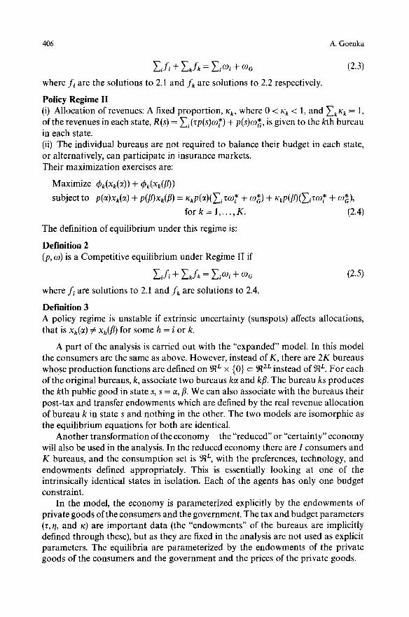
Z i f i + Y'.kfk = Zio91 + O9G (2.3)

where f i are the solutions to 2.1 and fk are solutions to 2.2 respectively.

Policy Regime II (i) Allocation of revenues: A fixed proportion, ~k, where 0 < ~k < 1, and ~.k ~k = l, of the revenues in each state, R(s) = ~i(zP(S)o9*) + p(s)o9*, is given to the kth bureau in each state. (ii) The individual bureaus are not required to balance their budget in each state, or alternatively, can participate in insurance markets. Their maximization exercises are:

Maximize ~Pk(Xk(~)) + ~k(Xk(fl))

subject to p(e)Xk(Ct) + p([3)Xk(fl) = Xkp(CO(~iZO9* + O9*) + Kkp(fl)(~rOg* + O9"),

for k = 1,. . . , K. (2.4)

The definition of equilibrium under this regime is:

Definition 2 (p, co) is a Competitive equilibrium under Regime II if

~,, f , + ~_,kfk = Z,Ogi + O9~ (2.5)

where fi are solutions to 2.1 and fk are solutions to 2.4.

Definition 3 A policy regime is unstable if extrinsic uncertainty (sunspots) affects allocations, that is Xh(~) ~ Xh(fl) for some h = i or k.

A part of the analysis is carried out with the "expanded" model. In this model the consumers are the same as above. However, instead of K, there are 2K bureaus whose production functions are defined on 9~ L x {0} c ~2L instead of 9~ L. For each of the original bureaus, k, associate two bureaus ks and kfl. The bureau ks produces the kth public good in state s, s = ~, ft. We can also associate with the bureaus their post-tax and transfer endowments which are defined by the real revenue allocation of bureau k in state s and nothing in the other. The two models are isomorphic as the equilibrium equations for both are identical.

Another transformation of the economy - the "reduced" or "certainty" economy will also be used in the analysis. In the reduced economy there are I consumers and K bureaus, and the consumption set is 9t L, with the preferences, technology, and endowments defined appropriately. This is essentially looking at one of the intrinsically identical states in isolation. Each of the agents has only one budget constraint.

In the model, the economy is parameterized explicitly by the endowments of private goods of the consumers and the government. The tax and budget parameters (z, t/, and ~:) are important data (the "endowments" of the bureaus are implicitly defined through these), but as they are fixed in the analysis are not used as explicit parameters. The equilibria are parameterized by the endowments of the private goods of the consumers and the government and the prices of the private goods.


3. Equilibria under Policy Regime I

In this section properties of the set of Competitive Equilibria under Regime I are examined. We establish existence of equilibrium for any endowment distribution,

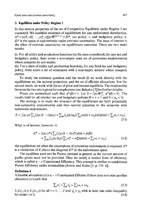
* * * = 12", tax policy, z, and budgetary policy, r/. CO* = (COl, CO2 . . . . ,CO, ,CO~)~L( '+ '~ O* is the space of endowments under extrinsic uncertainty. The issue of interest is the effect of extrinsic uncertainty on equilibrium outcomes. There are two main results.

(i) For all utility and production functions (in the class considered), for any tax and budgetary policy, there exists a non-empty open set of economies (endowments) where sunspots do not matter. (ii) For a class of utility and production functions, for any fixed tax and budgetary policy, there exists a set of economies with a non-empty interior where sunspots matter.

To study the existence question and the result (i) we work directly with the equilibrium set, the natural projection, and the set of efficient allocations. For the second result, we work with the set of price and income equilibria. The relationship between the two sets is given for completeness (see Balasko [3] for further details).

t ~ ~I~2L Prices are normalized such that pL(fl)= 1. Let S = (p ++:pL(fl)= 1}. The results hold for all interior tax and budgetary policies (0 < z < 1 and 0 < r/k < 1).

The strategy is to study the structure of the equilibrium set (with potentially non-symmetric endowments) and then restrict attention to the economy with symmetric endowments.

E = {(p, co):~,fi(p, (1 - z)pco,) + ~ksfk~(P, (nk(Z~COi(s) + COG(S)))P(S)) = ~iCOi + COG }" (3.1)

What is of interest, however, is:

E* = {(p, co*):~if/(p, (1 - z)co*(p(ct) + p(fl))

+ ~ksfks(P, Olk(r~CO* + CO;))p(s)) = ~,CO, + COG} (3.2)

the equilibrium set when the assumption of symmetric endowments is imposed. E* is a restriction of E above the diagonal I"2" in the endowment space.

The equilibria need not be Pareto optimal in general as the correct amount of public goods need not be provided. They do satisfy a weaker form of efficiency, which is called r / - z Constrained Efficiency. This concept is similar to conditional Pareto Efficiency under externalities (Arrow and Hahn [1, p. 135-6-].

Definition 4 A feasible allocation (x) is r / - z Constrained Efficient if there does not exist another allocation (x') such that

2iX' i "~- ~.~k Xk ~--- Ei(l)i "~- (D G (3.3)

Ui(x' i, y) > Ui(xi, y) for all i = 1 . . . . . I and Yk > Yk with at least one strict inequality for some i or k. (3.4)

408 A. Goenka

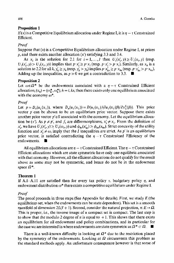
Proposition 1 If(x) is a Competitive Equilibrium allocation under Regime I, it is q - r Constrained Efficient.

Proof Suppose that (x) is a Competitive Equilibrium allocation under Regime I, at prices p, and there exists another allocation (x') satisfying 3.3 and 3.4.

As x i is the solution for 2.1 for i = 1 . . . . . I then U i ( x ' i , y ) > U ~ ( x i , y ) (resp. Ui(x'i, y ) > Ui(xi, y) ) implies that p. x ' i > p" x i (resp. p" x' i > p" xi). Similarly, as Xk is a solution to 2.2 for all k, Yk > Yk (resp. Yk > Yk) implies P" Xks > p" Xks (resp. p" X'ks > p" Xk~). Adding up the inequalities, as p >> 0 we get a contradiction to 3.3. �9

Proposition 2 Let oe .O* be the endowments associated with a ~ / - r Constrained Efficient allocation, (Xh) = (09~ , eg'~), h = i, ks, then there exists only one equilibrium associated with the economy o*.

Proof Let p = D,(u 1 (x , ) ) , where D,(u l (Xx)) = D ( u l ( x l ) / ( g u l ( x l (fl)/c3x~(fl)). This price vector p can be shown to be an equilibrium price vector. Suppose there exists another price vector p ' ~ S associated with the economy. Let the equilibrium allocation be (x'). As p # p', and fi are diffeomorphisms, x ' i v~ xi. From the definition of x i, we have Ui(xi , y) > Ui(oi , y) and C~k~(Xk~) _ ~ks(Xk~). Strict concavity of the utility function and x' i # ~ imply that the I inequalities are strict. As p' is an equilibrium price vector, is satisfied contradicting the ~/- z Constrained Efficiency of the endowments. �9

All equilibrium allocations are r / - z Constrained Efficient. The r / - z Constrained Efficient allocations which are state symmetric have only one equilibria associated with that economy. However, all the efficient allocations do not qualify for the result above as some may not be symmetric, and hence do not lie in the endowment space .(2"

Theorem 1 If A.1-A.11 are satisfied then for every tax policy z, budgetary policy ~/, and endowment distribution o9" there exists a competitive equilibrium under Regime I.

Proof The proof proceeds in three steps (See Appendix for details). First, we study E (the equilibrium set, when the endowments can be state dependent). This set is a smooth manifold of dimension 2L(I + 1). Second, consider the natural projection, n:E ~.(2. This is proper, i.e., the inverse image of a compact set is compact. The last step is to show that the modulo 2 degree of 7r is equal to + 1. This shows that there exists an equilibrium for all endowment and policy combinations, and in particular for the case we are interested in where endowments are state symmetric as O* ~ O. �9

There is a well-known difficulty in looking at .(2" due to the restriction placed by the symmetry of the endowments. Looking a t / 2 circumvents this problem as the standard methods apply. An unfortunate consequence however is that some of


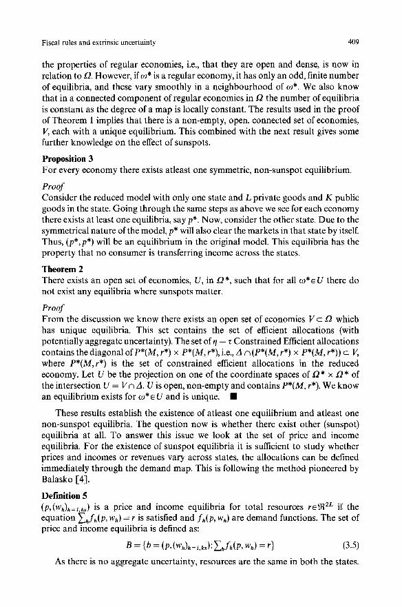
the properties of regular economies, i.e., that they are open and dense, is now in relation to 12. However, if to* is a regular economy, it has only an odd, finite number of equilibria, and these vary smoothly in a neighbourhood of 09*. We also know that in a connected component of regular economies in ~Q the number of equilibria is constant as the degree of a map is locally constant. The results used in the proof of Theorem 1 implies that there is a non-empty, open, connected set of economies, V, each with a unique equilibrium. This combined with the next result gives some further knowledge on the effect of sunspots.

Proposition 3 For every economy there exists atleast one symmetric, non-sunspot equilibrium.

Proof Consider the reduced model with only one state and L private goods and K public goods in the state. Going through the same steps as above we see for each economy there exists at least one equilibria, say p*. Now, consider the otfier state. Due to the symmetrical nature of the model, p* will also clear the markets in that state by itself. Thus, (p*, p*) will be an equilibrium in the original model. This equilibria has the property that no consumer is transferring income across the states.

Theorem 2 There exists an open set of economies, U, in I2", such that for all 09* ~ U there do not exist any equilibria where sunspots matter.

Proof From the discussion we know there exists an open set of economies V c ~ which has unique equilibria. This set contains the set of efficient allocations (with potentially aggregate uncertainty). The set ofq - z Constrained Efficient allocations contains the diagonal ofP*(M, r*) • P*(M, r*), i.e., A n(P*(M, r*) • P*(M, r*)) c V, where P*(M,r*) is the set of constrained efficient allocations in the reduced economy. Let U be the projection on one of the coordinate spaces of O* • ~ * of the intersection U = Vn A. U is open, non-empty and contains P*(M, r*). We know an equilibrium exists for o~*~ U and is unique. �9

These results establish the existence of atleast one equilibrium and atleast one non-sunspot equilibria. The question now is whether there exist other (sunspot) equilibria at all. To answer this issue we look at the set of price and income equilibria. For the existence of sunspot equilibria it is sufficient to study whether prices and incomes or revenues vary across states, the allocations can be defined immediately through the demand map. This is following the method pioneered by Balasko I-4].

Definition 5 (p,(Wh)h=i, ks ) is a price and income equilibria for total r e s o u r c e s r ~ l ~ 2L if the equation ~hfh(P, Wh) = r is satisfied and fh(P, Wh) are demand functions. The set of price and income equilibria is defined as:

B = {b = (p, (Wh)h=i, ks):~hfh(p, Wh) = r} (3.5)

As there is no aggregate uncertainty, resources are the same in both the states.

410 A. Goenka

This implies that we restrict our attention to:

Bs = {b = (p, (Wh)h=i, ks):F(b) = ~ n f h ( P , Wh) is symmetric} (3.6)

Till now the "incomes" of the bureaus do not correspond to the budgetary policy r/. The budgetary policy imposes restrictions on the incomes of the bureaus: they have to be proportional in a specific way.

Definition 6 The set of price and income equilibria consistent with policy regime I is:

Bs(rl) = {b~B~:WkJWh~ = rlk/q h for s = c~, fl and all h ~ k} (3.7)

The set of price and income equilibria where sunspots do not matter is:

B's(rl ) = {beB~(rl ) :b is symmetric} (3.8)

We can define a map 2:E* ~ B as follows:

2(p, (e)i) i , (09k~)ks) = (p, (p" ~0i) i, (p'O)ks)k,) (3.9)

NOW, 2(E*)=Bs(r/). Similarly, we can look at 2 : E * * ~ B , where E * * = {(p,e))e E*:p(ct) = p(fl)}, and note that 2(E**) c B'(r/).

The strategy is to show there exist points in B that belong to image of E* but not to the image of E** through the map 2. The map 2, it should be noted, is neither onto nor one-to-one. The definition of the price and income equilibria does not have any notion of endowments associated with it. Thus, we have to check compatibility of these equilibria with symmetric endowments. Finding symmetric endowments for symmetric equilibria is straightforward. We have the following result.

Proposition 4 A sufficient condition for the compatibility of symmetric endowments with the asymmetric price and income equilibria is that the prices in the two states are not collinear.

P r o o f The existence of the symmetric endowments of the bureaus, given t/k, is the same as the existence of symmetric endowments for the government and the individual consumers. For the endowments of the government we have to find a solution co*'-- co~ + Zivco* to

p(~).~o*' = wG(~)

p(fl)'~o*' = ~%(fl) (3.10)

A solution exists if and only if P (p )= [p(e)p(f l)-I ' and R(b)= [P(p)e)G] have the same rank (Kronecker-Capelli Theorem). This is always true if L > 2 and rank(P(b)) = 2.

For i = 2 . . . . . I solve the following equation for o)i:

(1 - ~ ) ( p ( ~ ) + p(/~))o~* = w, (3 .11 )

These (co i , co i ) are the symmetric endowments for the i ~ 1 consumers. Let r = F(b) =


(F(b)*, F(b)*) be the symmetric total aggregate demand associated with beB s. Define

(1 - z)tol = r - ~ i , 1( 1 - z ) to i - to'G (3.12)

By construction tol = (to*, to*) is symmetric�9 For the endowments to be compatible with b, it must be the case that ( 1 - z)(p(ct)+ p(fl))to* = wl. Multiply (3�9 by (p(~) + p(fl)) then,

(1 - z)(p(e) + p(fl))to~ = (p(e) + p(f l))(F(b)* - ~ i e i wirn* - - WGe'~*'~l

= w 1 (by Walras' law).

Now define to* = to*' - - "t~,i(.o~ �9 �9

Proposi t ion 5 For a given tax policy z and budget policy r/if A.1-A.5 and A.7-A.10 are satisfied, the set of price and income equilibria B~(r/) is a smooth submanifold of dimension

2L - 1 ~ I + 2K�9 (L + I + 1) of 9~+4. • The set of symmetric price and income equilibria B'~0I) is a smooth submanifold of B~(r/) of dimension (L + I) diffeomorphic to

L - 1 ~ I + 1 ~ + + X �9

Proof By taking derivatives with respect to prices and incomes, it is easy to show that

�9 2L ~I4-2K__. ~ 2 L F.9t4. + x is a submersion (the tangent map is surjective) where F is the aggregate excess demand map (see Balasko [4, Lemma 5] for details)�9 Initially prices are not normalized�9

To calculate the dimension of B~, let A = {(x(0t), X(fl))e912L:x(CO = X(fl)}. F is transversal to A. Note that F - I(A) = B~ and dim (~++EL X ~ 1 + 2K) - - dim (F- I(A)) = dim (9t 2L) - dim (A) or

d im(F- ~(A)) = 2L+ I + 2K - ( 2 L - L)

= L + I + 2 K .

We can now normalize prices so that dim(B~) is (L+ I + 2 K - 1). Consider the inclusion map t: B~ ~ B(r/) where B(r/) = {beB: WkJWh~ = rlk/rlh}, dim B(~/) = 2L + 2. Notice that the set B~(r/) = B~ n B(r/). It is easy to check that B~ is transverse to B(r/), and Tb(B~) + Tb(B(rl)) = Tb(B). This implies that their intersection is also a submanifold (see Guillemin and Pollack [14]) and codim (B s n B(r/))= codim (Bs)+ codim (B(r/)). This can be further simplified to: dim (B~ n B0/)) = L + ! + 1.

For the second part of the proposition, consider the map z:B'~(rl)~ B*(~l), where B*(r/) is the set of price-income equilibria (consistent with the budgetary policy) in

' W' * * * p* the reduced economy. Z(P,( h))=(P ,(WR),(Wi )), where =p'(~)=p'(fl) and w k* = WRy' = WkaW* = WJ2: we associate with the symmetric price and income equilibria, the price and income equilibria in the reduced economy�9 The map is bijective. The inverse map ~ :B*(r/)~ B' (r/) is defined as follows: ~b(p*, (w*), (w*)) =

' W' W' p ' (P,( i),(ks)) where =(p*,p*), w'i=2w* and w' - w ' =w* Thus, ~k is an ket - - k f l k "

immersion (D~ is injective). It also takes its values in Bs(t/). It is thus an embedding r L--I ~ I + 1 and therefore, B~(t/) is a smooth submanifold diffeomorphic to ~Jl+4 . x

(Guillemin and Pollack [14, p. 17]). �9

A consequence is the following result.

412 A. Goenka

Corollary 1 The set of asymmetric price-income equilibria Bs(r/)\B's(rl) is a non-empty open subset of Bs(r/). In fact, B'~(q) is a lower dimensional subset of Bs(q).

Ideally we would like to show properties of B~(t/)\B", where B" is the set of price and income equilibria without collinear prices (placing no restriction on incomes). However, we cannot compute the dimension or properties of this set as B" is not a lower dimensional submainifold of B,(q). The result we have, is as a consequence weaker in that some points in the set Bs(~I)\B'~(rl) may not be compatible with symmetric endowments.

The issue remains whether the sufficient condition is non-vacuous. Again following the construction in Balasko [4, p. 41-43] we see that it is not. The preferences and technologies used are robust, the technologies are in fact chosen to be homothetic. It should be clear from the construction that the sunspot equilibria are not just randomizations over multiple certainty equilibria: there are sufficient degrees of freedom in the construction to allow consumers to transfers wealth across the states.

Proposition 6 There exist preferences and technologies which generate price-income equilibria, such that the rank of the matrix P(b) is maximal.

Proof See Appendix

Alternatively, for a wider class of preferences and technologies it is known that in the certainty economy there will be multiple equilibria (See Arrow and Hahn [1, Ch. 9]). These multiple equilibria arise for a connected set of economies (indexed by endowments) which have a non-empty interior. If there are multiple equilibria for a (regular) economy, there will be a neighbourhood of the economy where the number of equilibria is the same. Recognizing that a sunspot equilibrium can be a randomization over certainty equilibria, we have the following result.

Theorem 3 The Policy Regime I is unstable, i.e., there exists a class of preferences and technologies, and a set of economies (endowments) with a non-empty interior which has equilibria where extrinsic uncertainty matters.

The construction of sunspot equilibria is given as one would like to emphasize that existence of multiple certainty equilibria is only a sufficient condition.

4. Equilibria under Regime II

In this section policies which stabilize the economy are examined. When these policies are adopted the equilibria are necessarily symmetric. Under the stabilizing regime, the bureaus and the government have greater flexibility in pursuing their objectives as they have access to the insurance markets. Moreover, under this regime the conditions that characterize Pareto efficiency in public goods economies (Samuelson [18]), will in general not be satisfied. Thus, in a class of models where the equilibria are not Pareto efficient, there do not exist any sunspot equilibria. This


contrasts with the results in Cass and Shell I-7] and Cass and Polemarchakis [6] where the sufficient condition for extrinsic uncertainty not affecting equilibrium outcomes is ex-ante Pareto efficiency.

Definition 7 A feasible allocation (x) is said to be x Constrained Efficient if there does not exist an alternative allocation (x') such that

Eix'i + ZkX'k = ZiCOi + O0~ (4.1)

Ui(x' i, y) > Ui(x i, y) for all i and yk(~) + Yk(fl) > yk(~) + yk([3) for all k with at least one strict inequality for i or k. (4.2)

It should be clear that • Constrained Efficiency implies q - z Constrained Efficiency. In the original model the symmetric equilibria are precisely the allocations which satisfy this stronger concept of efficiency.

As the focus of the paper is the study of the symmetry property of the equilibria, one must show that they exist for all combinations of the endowments and budgetary policies. This can be done in two different ways: the first is as mentioned above. The symmetric equilibria under the first Policy Regime, are also equilibria under the second regime if the vector of allocations x = q, and from the previous section we know that there always exists a symmetric equilibrium. The second approach, is to look at the model, and recognizing that the public good plays the role of a non-traded consumption externality, apply Theorem 6.2 in Arrow and Hahn 1-1, p. 135]. The assumption of consumption sets being bounded from below is replaced by the assumption of indifference surfaces being bounded from below.

Theorem 4 If A.1-A.11 are satisfied then for every tax policy z and every budgetary policy x and endowment distribution ~o* there exists a competitive equilibrium under Regime II.

Proposition 7 If (x) is an equilibrium allocation under Regime II, it is ~ Constrained Efficient.

Proof Suppose that (x) is an equilibrium allocation at prices p which is not K Constrained Efficient. Then there exists another allocation (x') satisfying 4.1 and 4.2.

As xi is the solution to 2.1 for i = 1 . . . . . 1, then U~(x'~,y)> Ui(x~,y) (resp. Ui(x'i, y) > U~(xi, y) ) implies that p" x'i > p" xl (resp. p. x ' i > p" xi). Similarly, as Xk is a solution to 2.4 for k = 1 , . . . , K, yk(Ct) + Y'k(fl) > Yk(ct) + Yk(fl) (resp. y'k(~) + Y'k(fl) > yk(Ct) + yk([3)) implies that p ' x k > P'Xk (resp. p" x k > p" Xk). Adding up the inequalities, together with p >> 0 leads to a contradiction of 4.1. �9

Proposition 8 If (x) is ~ Constrained Efficient, it is symmetric.

Proof Suppose that (x) is a x Constrained Efficient allocation with either xi(ct ) ~ xi(fl) for some i or Xk(a) 4: Xk([3) for some k, or both. Consider the symmetric alternative allocation, (x' i, x'i) = (x i ( , ) + xi(fl)/2, xi(ct) + x~(fl)/2), (x k, Xk) = (Xk(~) + Xk([3)/2,

414 A. Goenka

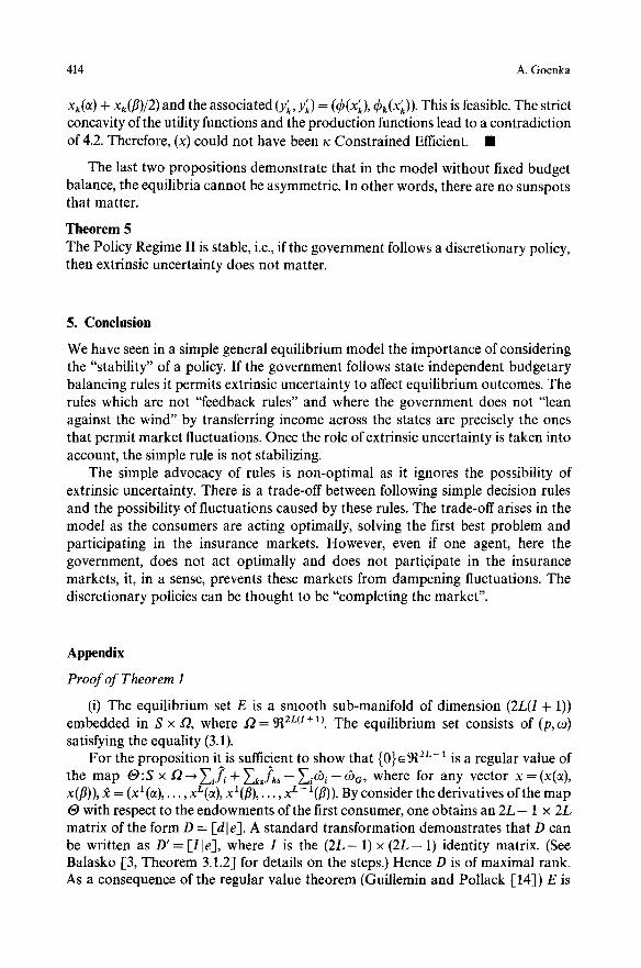
xk(~) + Xk(fl)/2) and the associated (Yk, Yk) = (~b(Xk), CPk(Xk))" This is feasible. The strict concavity of the utility functions and the production functions lead to a contradiction of 4.2. Therefore, (x) could not have been ~ Constrained Efficient. �9

The last two propositions demonstrate that in the model without fixed budget balance, the equilibria cannot be asymmetric. In other words, there are no sunspots that matter.

Theorem 5 The Policy Regime II is stable, i.e., if the government follows a discretionary policy, then extrinsic uncertainty does not matter.

5. Conclusion

We have seen in a simple general equilibrium model the importance of considering the "stability" of a policy. If the government follows state independent budgetary balancing rules it permits extrinsic uncertainty to affect equilibrium outcomes. The rules which are not "feedback rules" and where the government does not "lean against the wind" by transferring income across the states are precisely the ones that permit market fluctuations. Once the role of extrinsic uncertainty is taken into account, the simple rule is not stabilizing.

The simple advocacy of rules is non-optimal as it ignores the possibility of extrinsic uncertainty. There is a trade-off between following simple decision rules and the possibility of fluctuations caused by these rules. The trade-off arises in the model as the consumers are acting optimally, solving the first best problem and participating in the insurance markets. However, even if one agent, here the government, does not act optimally and does not participate in the insurance markets, it, in a sense, prevents these markets from dampening fluctuations. The discretionary policies can be thought to be "completing the market".

Appendix

Proof of Theorem I

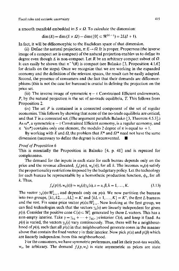
(i) The equilibrium set E is a smooth sub-manifold of dimension (2L(I + 1)) embedded in S • ~, where ~ = ~2ut+l). The equilibrium set consists of (p,m) satisfying the equality (3. I).

For the proposition it is sufficient to show that {0} ~9t 2L- 1 is a regular value of the map O:S x s ~ i f i + ~ksfks- ~i~bi- a3o, where for any vector x = (x(a), x(fl)), ~ = (x l (~) , . . . , xL(~), xl(/~), . . . , x L- l(fl)). By consider the derivatives of the map O with respect to the endowments of the first consumer, one obtains an 2L-- 1 x 2L matrix of the form D = Id[ e]. A standard transformation demonstrates that D can be written as D ' = [I[e], where I is the ( 2 L - 1 ) x ( 2 L- 1 ) identity matrix. (See Balasko I-3, Theorem 3.l.2] for details on the steps.) Hence D is of maximal rank. As a consequence of the regular value theorem (Guillemin and Pollack [14]) E is


a smooth manifold embedded in S x 12. To calculate the dimension:

dim (E) = dim (S x 12) - dim ({0} c 9{ 2L- 1) = 2L(I + 1).

In fact, it will be diffeomorphic to the Euclidean space of that dimension. (ii) Define the natural projection, n: E ~ 12. It is proper. Properness (the inverse

image of a compact set is compact) of the natural projection enables us to define its degree even though E is non-compact. Let R be an arbitrary compact subset of 12. It can easily be shown that rt-I(R) is compact (see Balasko [3, Proposition 4.1.6] for details on the steps). Once we recognize that we are working in the expanded economy and the definition of the relevant spaces, the result can be easily adapted. Second, the presence of consumers and the fact that their demands are diffeomorphisms (this is not the case for bureaus) is crucial in defining the projection on the price set.

(iii) The inverse image of symmetric t / - ~ Constrained Efficient endowments, P, by the natural projection is the set of no-trade equilibria, T. This follows from Proposition 2.

(iv) The set P is contained in a connected component of the set of regular economies. This follows by showing that none of the no-trade equilibria are critical, and that T is a connected set. (The argument parallels Balasko [3, Theorem 4.5.3].) As c9", a symmetric r / - z Constrained Efficient economy, is a regular economy, and rt- 1(~,) contains only one element, the modulo 2 degree of n is equal to + 1.

By working with E and 12, the problem that E* and 12" need not have the same dimension (necessary to define the degree) is circumvented. �9

Proof of Proposition 6 This is essentially the Proposition in Balasko [4, p. 41] and is repeated for completeness.

The demand for the inputs in each state for each bureau depends only on the price and the revenue allocated, fk(p(s), Wk(S)), for all k. The incomes Wk(S) satisfy the proportionality restrictions imposed by the budgetary policy. Let the technology for each bureau be representable by a homothetic production function, ~bk, for all k. Thus,

f k ( p ( s ) , Wk(S)) = Wk(S)•k(S), S = 0~, fl, k = 1 . . . . , K. (3.13)

The vector 7k(S)~IL++, and depends only on p(s). We now partition the bureaus into two groups, {kl, k2 . . . . . kL} = K' and {kL + 1 . . . . , K} = K", the first L bureaus and the rest. Fix some price vector p(s)~L++. Now looking at the first group, we can find technologies such that the vectors 7k(s) are linearly independent for given p(s). Consider the positive cone C(s) c 9tL+ generated by these L vectors. This has a non-empty interior. Take 7 = 7kl + " ' " "q- ])kL, 7~interior C(s), and keep it fixed. As p(s) is varied, the vectors ~k(S) vary continuously. Thus, there will be a neighbourhood of p(s), such that all if(s) in that neighbourhood generate cones in the manner above that contain the fixed vector 7 in their interior. Now pick p(a) and p(fl) which are linearly independent from this neighbourhood.

For the consumers, we have symmetric preferences, and let their post-tax wealth, wl, be arbitrary. The demand fi(P, wi) is state asymmetric as prices are state

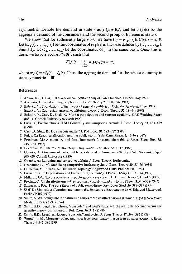
416 A. Goenka

asymmetric. Denote the demand in state s as f i(P, wl)(s), and let F(p)(s) be the aggregate demand of the consumers and the second group of bureaus in state s.

We show that for sufficiently large v > 0, we have (v7 - F(p)(s))eC(s) , s = ~, ft. Let ((kl (S), . . . , (kL(S)) be the coordinates of F(p)(s) in the base defined by (7~1 . . . . , ~kL)" Similarly, let (r . . . . . ~kL) be the coordinates of 7 in the same basis. Once this is done, we have a vector r*~ 9t L, such that

F(p)(s) + ~ Wk(S)Tk(S ) = r*, k~K"

where Wk(S ) = V(k(S) -- (k(S). Thus, the aggregate demand for the whole economy is state symmetric. �9

References

1. Arrow, K.J., Hahn, F.H.: General competitive analysis. San Francisco: Holden Day 1971 2. Azariadis, C.: Self-Fulfilling prophecies. J. Econ. Theory 25, 380-396 (1981) 3. Balasko, Y.: Foundations of the theory of general equilibrium. Orlando: Academic Press 1988 4. Balasko, Y.: Equivariant general equilibrium theory. J. Econ. Theory 52, 18-44 (1990) 5. Balasko, Y., Cass, D., Shell, K.: Market participation and sunspot equilibria. CAE Working Paper

#88.11, Cornell University (revised) 1990 6. Cass, D., Polemarchakis, H.M.: Convexity and sunspots: a remark. J. Econ. Theory 52, 433-439

(1990) 7. Cass, D., Shell, K.: Do sunspots matter? J. PoE Econ. 91, 193-227 (1983) 8. Foley, D.: Resource allocation and the public sector. Yale Econ. Essays 7, 45-98 (1967) 9. Friedman, M.: A monetary and fiscal framework for economic stability. Amer. Econ. Rev. 38,

245-264 (1948) 10. Friedman, M.: The role of monetary policy. Amer. Econ. Rev. 58, 1-17 (1968) 11. Goenka, A: Government rules, public goods, and extrinsic uncertainty. CAE Working Paper

#89-20, Cornell University (1989) 12. Goenka, A.: Rationing and sunspot equilibria. J. Econ. Theory, forthcoming 13. Grandmont, J.-M.: Stabilizing competitive business cycles. J. Econ. Theory 40, 57-76 (1986) 14. Guillemin, V., Pollack, A.: Differential topology. Englewood Cliffs: Prentice Hall 1974 15. Lucas Jr., R.E.: Expectations and the neutrality of money. J Econ. Theory 4, 103-124 (1972) 16. Milleron, J.-C.: Theory ofvalue with public goods: a survey article. J. Econ. Theory 5, 419-477 (1972) 17. Pr6chac, C.: On the effectiveness ofsunspots in incomplete markets. Econ. Theory 3, 585-588 (1993) 18. Samuelson, P.A.: The pure theory of public expenditure. Rev. Econ. Stud. 36, 387-389 (1954) 19. Shell, K.: Monnaie et allocation intertemporelle. Seminaire d'Econometrie de M. Edmond Malinvaud.

Paris: CNRS (1977) 20. Smith, A.: An inquiry into the nature and causes ofthe wealth ofnations. (Cannan, E. (ed.)) New York:

Modern Library 1937 (1776) 21. Smith, B.D.: Legal restrictions, "sunspots," and Peel's bank act: the real bills doctrine versus the

quantity theory reconsidered. J. Pol. Econ. 96, 3-19 (1986) 22. Smith, B.D.: Legal restrictions, "sunspots," and cycles. J. Econ. Theory 47, 369-392 (1989) 23. Woodford, M.: Monetary policy and price level determinacy in a cash-in-advance economy. Econ.

Theory 4, 345-380 (1994)

Fiscal rules and extrinsic uncertainty

Documents

Transcript of Fiscal rules and extrinsic uncertainty