Lecture 1I: tensor network algorithms (iPEPS)
60
Lecture 1I: tensor network algorithms (iPEPS) Philippe Corboz, Institute for Theoretical Physics, University of Amsterdam
-
Upload
khangminh22 -
Category
Documents
-
view
0 -
download
0
Transcript of Lecture 1I: tensor network algorithms (iPEPS)

Lecture 1I: tensor network algorithms(iPEPS)
Philippe Corboz, Institute for Theoretical Physics, University of Amsterdam

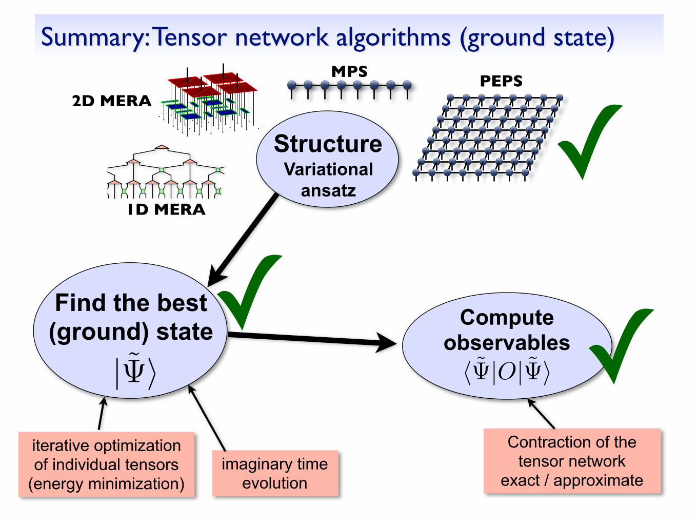
Overview: Tensor network algorithms (ground state)
iterative optimization of individual tensors
(energy minimization)imaginary time
evolution
Contraction of the tensor network
exact / approximate
Find the best (ground) state
|��
Compute observables��|O|�⇥
MPS PEPS2D MERA
1D MERA
TN ansatz (variational)

Contracting a tensor network

Pairwise contractions...
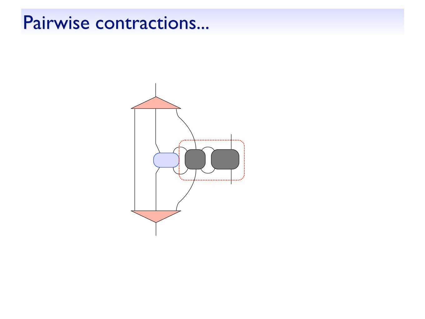
Pairwise contractions...
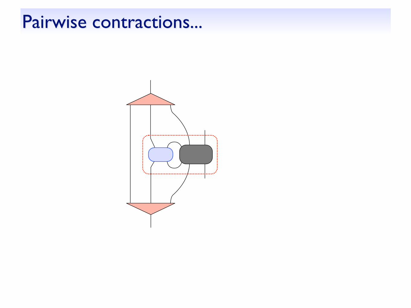
Pairwise contractions...

Pairwise contractions...

Pairwise contractions...

Pairwise contractions...
done!
the order of contraction matters for the computational cost!!!
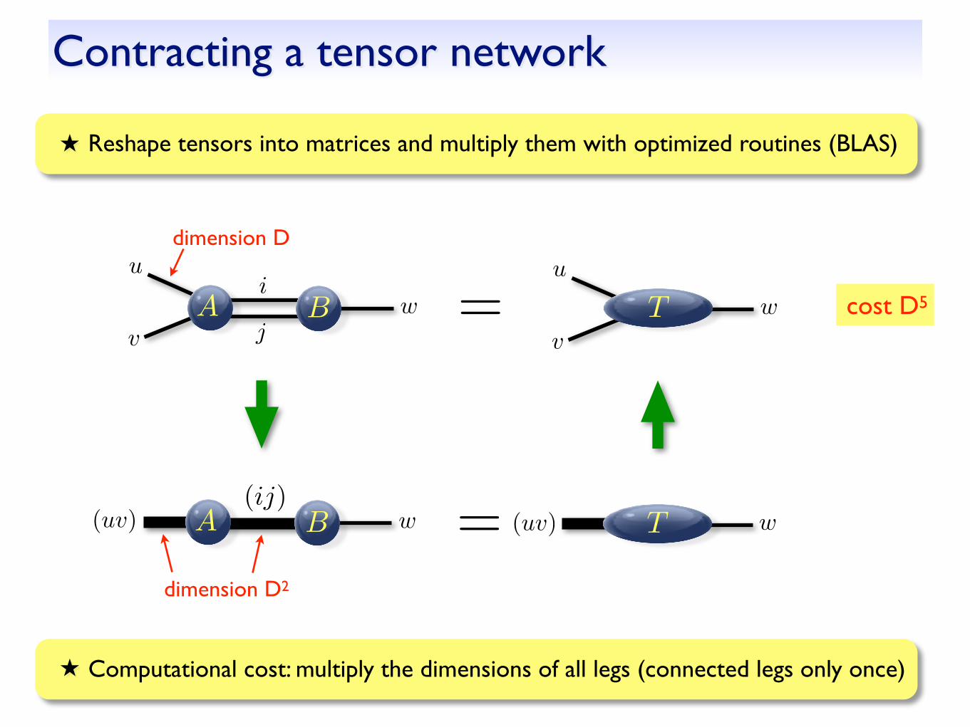
Contracting a tensor network
★ Reshape tensors into matrices and multiply them with optimized routines (BLAS)
i
j
u
vA B w =
u
v
wT
= wT(uv)
dimension D
★ Computational cost: multiply the dimensions of all legs (connected legs only once)
cost D5
B w(uv) A(ij)
dimension D2

Contraction: Example from the 2D MERA
w1 w2 w3 w4
uux uy
� (lower half)
� (upper half)
H
What is the optimal contraction order?
Use program to find optimal contraction, e.g. NETCON:
Pfeifer, Haegeman, Verstraete, PRE 90 (2014)
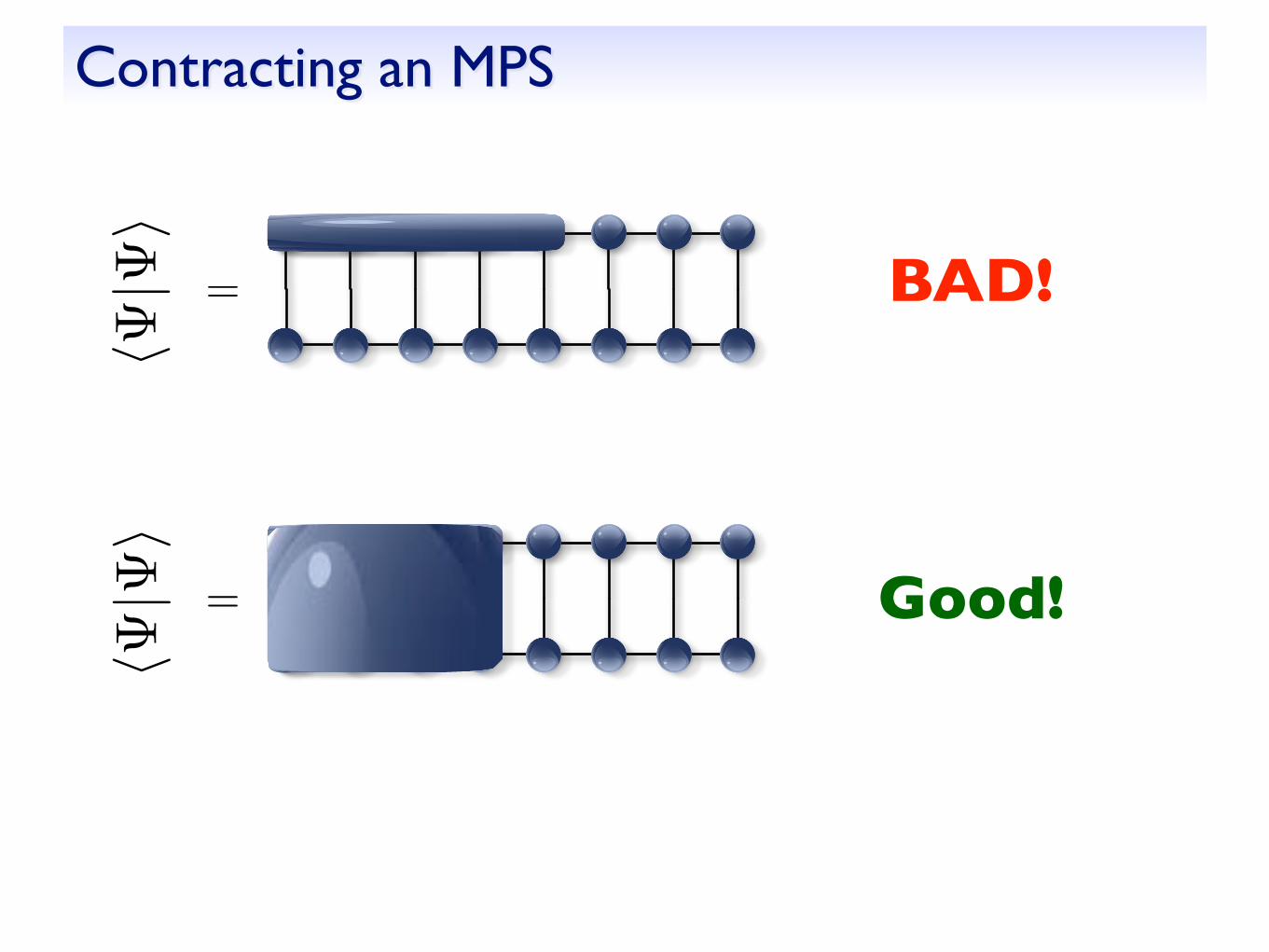
Contracting an MPS��
|�⇥
= BAD!
��|�
⇥
= Good!

MERA: Contraction
��|
Let’s compute ��|O|�⇥ O : two-site operator
|��
O two-site operator
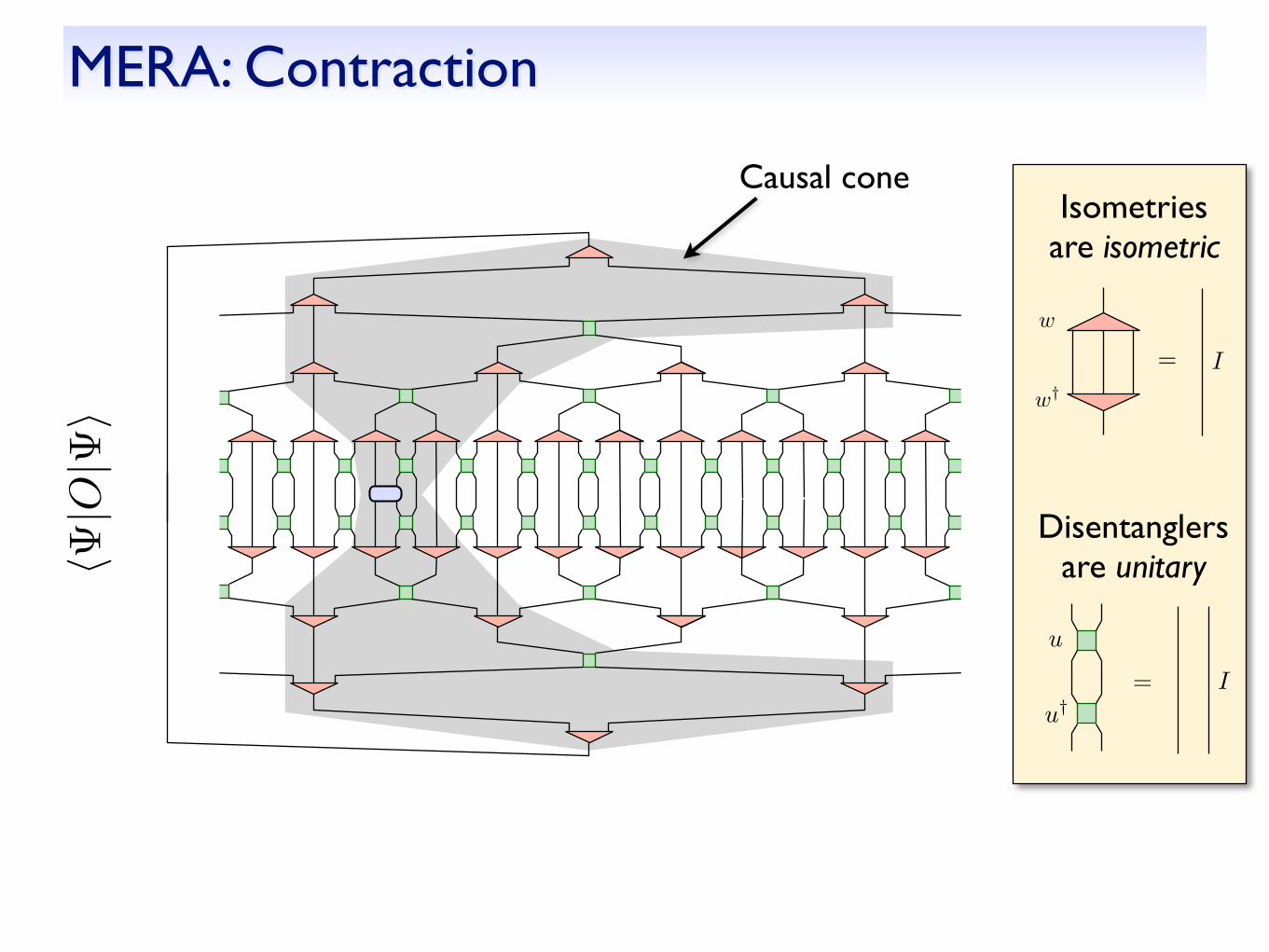
Causal cone
MERA: Contraction��
|O|�
⇥
Isometries are isometric
= I
u
u†
= I
w
w†
Disentanglers are unitary

MERA: Contraction��
|O|�
⇥
Causal cone
Efficient computation of expectation values of observables!
Isometries are isometric
= I
u
u†
= I
w
w†
Disentanglers are unitary
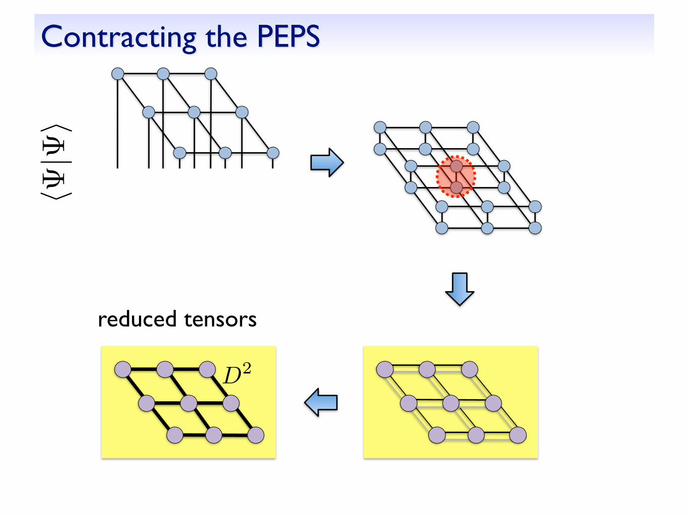
Contracting the PEPS��
|�⇥
reduced tensors
D2

Contracting the PEPS
Problem: how do we contract this??
no matter how we contract, we will get intermediate
tensors with O(L) legs
number of coefficients D2L Exponentially increasing with L!
NOT EFFICIENT
dimension D2

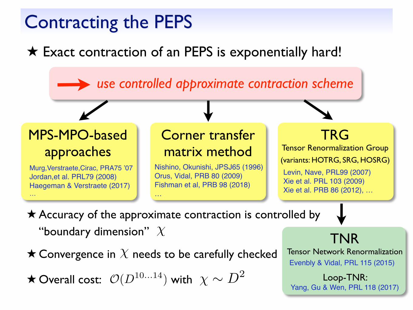
Contracting the PEPS★ Exact contraction of an PEPS is exponentially hard!
use controlled approximate contraction scheme
MPS-MPO-based approaches
Corner transfer matrix method
TRG Tensor Renormalization Group(variants: HOTRG, SRG, HOSRG)
Murg,Verstraete,Cirac, PRA75 ’07Jordan,et al. PRL79 (2008)Haegeman & Verstraete (2017)…
Nishino, Okunishi, JPSJ65 (1996)Orus, Vidal, PRB 80 (2009)Fishman et al, PRB 98 (2018)…
Levin, Nave, PRL99 (2007)Xie et al. PRL 103 (2009)Xie et al. PRB 86 (2012), …
★Accuracy of the approximate contraction is controlled by “boundary dimension” �
★Convergence in needs to be carefully checked�
★Overall cost: with � ⇠ D2O(D10...14)
TNRTensor Network Renormalization
Loop-TNR: Yang, Gu & Wen, PRL 118 (2017)
Evenbly & Vidal, PRL 115 (2015)

Contracting the PEPS
0 0.02 0.04 0.06 0.08 0.1−0.6695
−0.669
−0.6685
1/χ
E s
D=4D=5D=6
Example: 2D Heisenberg model (CTM)
★ Be careful with “variational” energy!!!
★ Fast convergence
★ Effect of finite D is much larger!

Contracting the PEPS★ Exact contraction of an PEPS is exponentially hard!
use controlled approximate contraction scheme
MPS-MPO-based approaches
Corner transfer matrix method
TRG Tensor Renormalization Group(variants: HOTRG, SRG, HOSRG)
Murg,Verstraete,Cirac, PRA75 ’07Jordan,et al. PRL79 (2008)Haegeman & Verstraete (2017)…
Nishino, Okunishi, JPSJ65 (1996)Orus, Vidal, PRB 80 (2009)Fishman et al, PRB 98 (2018)…
Levin, Nave, PRL99 (2007)Xie et al. PRL 103 (2009)Xie et al. PRB 86 (2012), …
★Accuracy of the approximate contraction is controlled by “boundary dimension” �
★Convergence in needs to be carefully checked�
★Overall cost: with � ⇠ D2O(D10...14)
TNRTensor Network Renormalization
Loop-TNR: Yang, Gu & Wen, PRL 118 (2017)
Evenbly & Vidal, PRL 115 (2015)
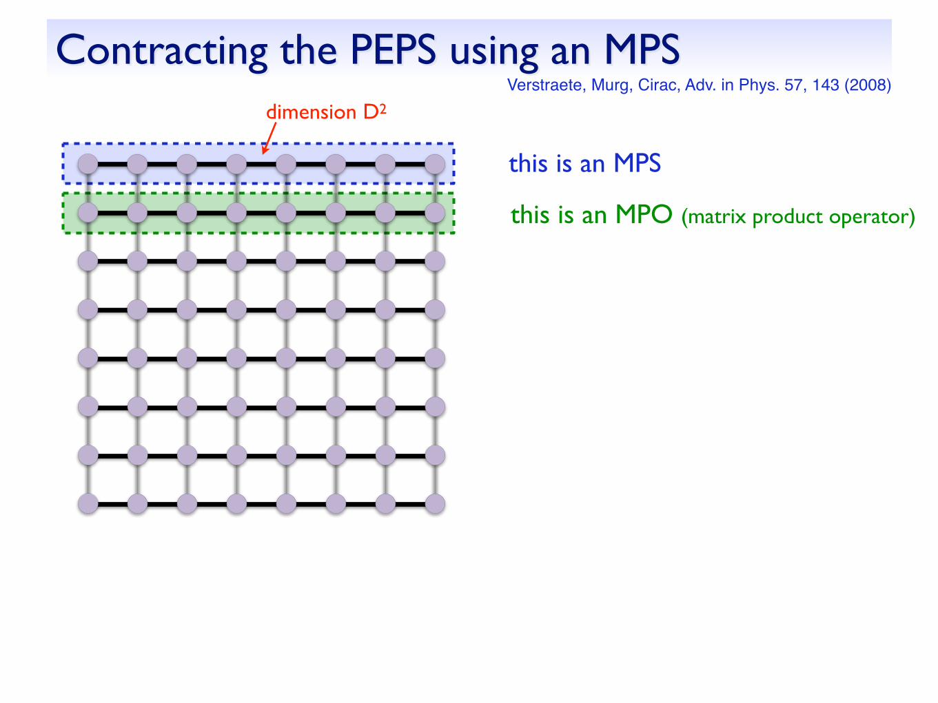
this is an MPO (matrix product operator)
this is an MPS
Contracting the PEPS using an MPSdimension D2
Verstraete, Murg, Cirac, Adv. in Phys. 57, 143 (2008)

Contracting the PEPS using an MPS
this is an MPS with bond dimension D2 xD2
dimension D2xD2
truncate the bonds to �
there are different techniques for the efficient MPO-MPS multiplication (SVD, variational optimization, zip-up algorithm...)Schollwöck, Annals of Physics 326, 96 (2011)Stoudenmire, White, New J. of Phys. 12, 055026 (2010).
Verstraete, Murg, Cirac, Adv. in Phys. 57, 143 (2008)

Contracting the PEPS using an MPS
dimension �
proceed...
★ We can do this from several directions★ Similar procedure when computing an expectation value
Verstraete, Murg, Cirac, Adv. in Phys. 57, 143 (2008)
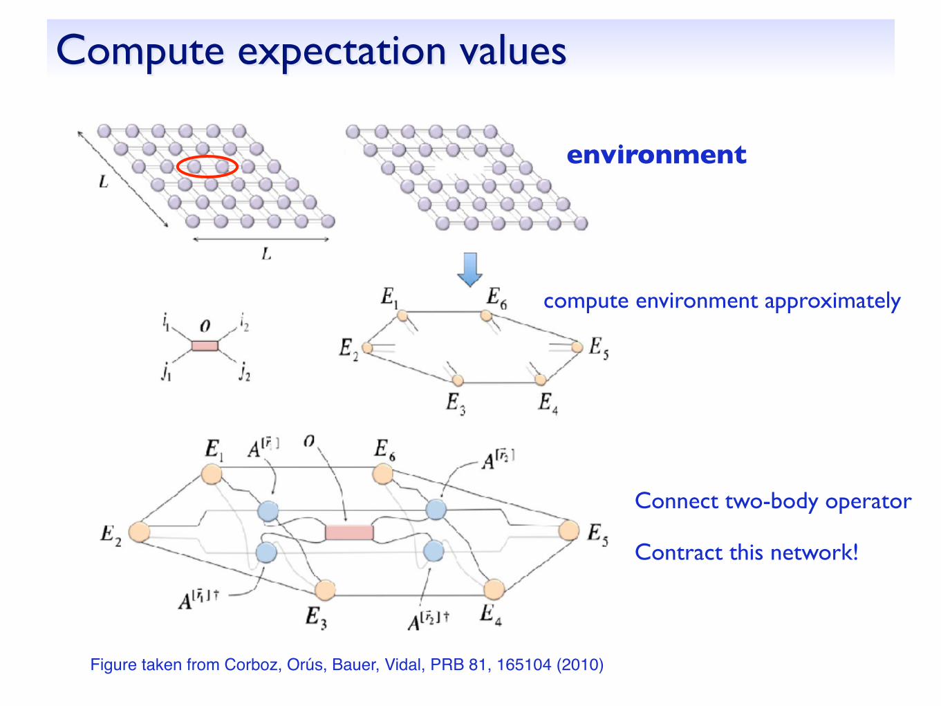
Compute expectation values
Figure taken from Corboz, Orús, Bauer, Vidal, PRB 81, 165104 (2010)
environment
compute environment approximately
Connect two-body operator
Contract this network!
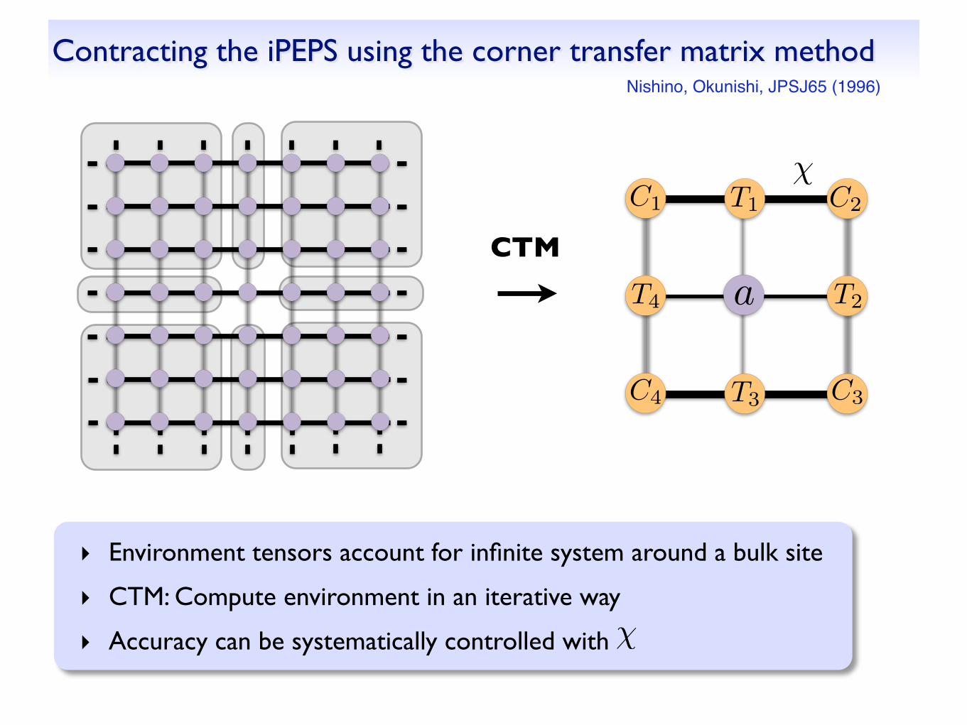
Contracting the iPEPS using the corner transfer matrix method
‣ Environment tensors account for infinite system around a bulk site
‣ CTM: Compute environment in an iterative way
‣ Accuracy can be systematically controlled with �
CTMa
C1
T3
T4
T1
C3
T2
C4
C2
�
Nishino, Okunishi, JPSJ65 (1996)
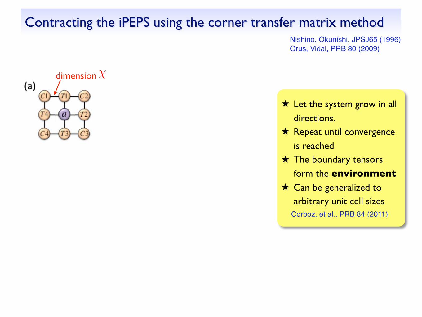
figure taken from Orus, Vidal, PRB 80 (2009)
Nishino, Okunishi, JPSJ65 (1996)Orus, Vidal, PRB 80 (2009)
★ Let the system grow in all directions.
★ Repeat until convergence is reached
★ The boundary tensors form the environment
★ Can be generalized to arbitrary unit cell sizes
Corboz, et al., PRB 84 (2011)
dimension �
Contracting the iPEPS using the corner transfer matrix method
C’ T’
T’ a
� D2C’
T’
C’C’ T’
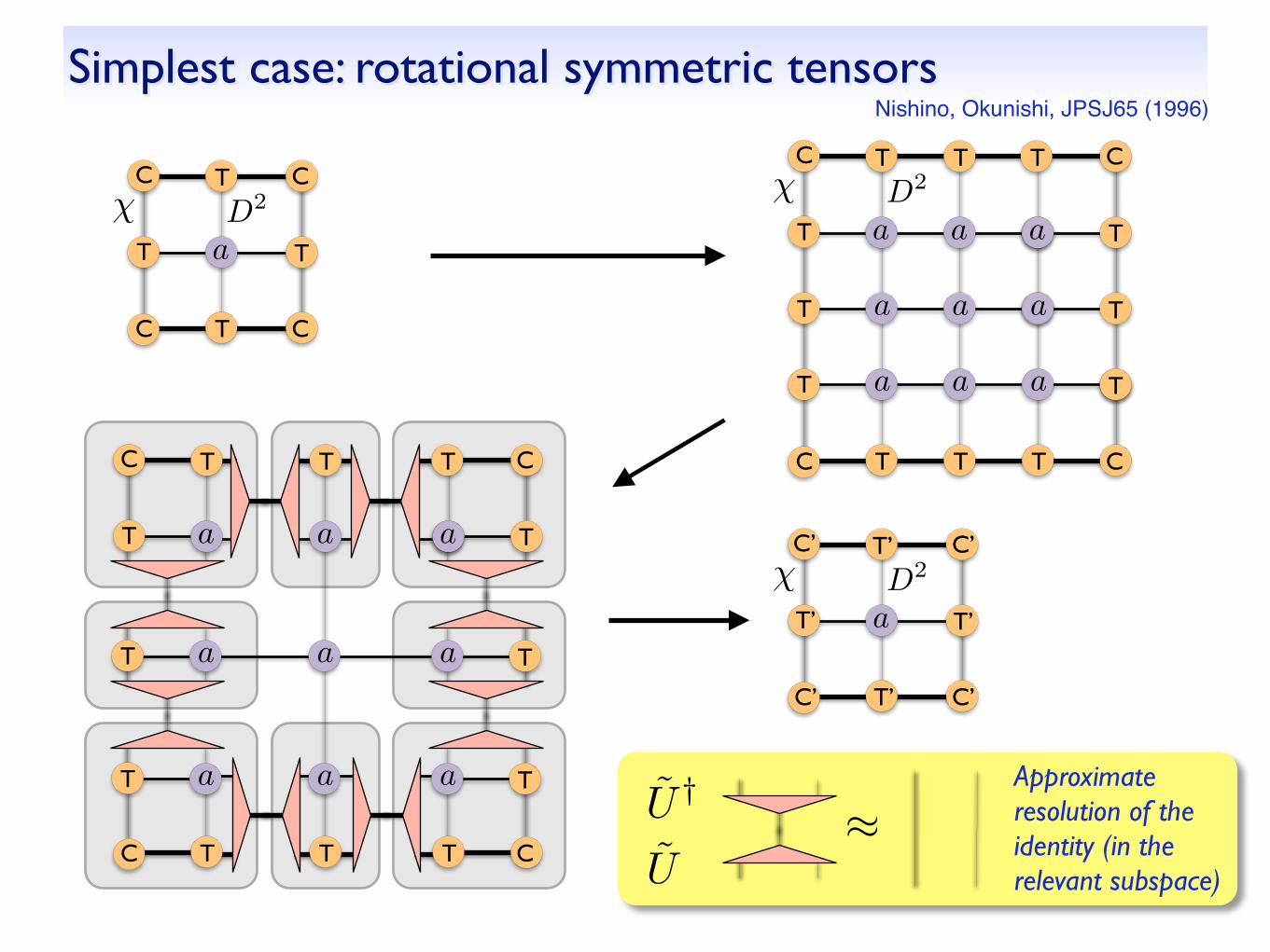
Simplest case: rotational symmetric tensors Nishino, Okunishi, JPSJ65 (1996)
C T
T a
� D2C
T
CC T
C
T
T
T T
T
T
a a
aa
� D2
C
C
T
T
a
a
aa
C
TaT
C T T T
T
C
T
T T
T a a
C
Ta
T aa Ta
CC T T T
T
T aa Ta
U
U †⇡
Approximate resolution of the identity (in the relevant subspace)
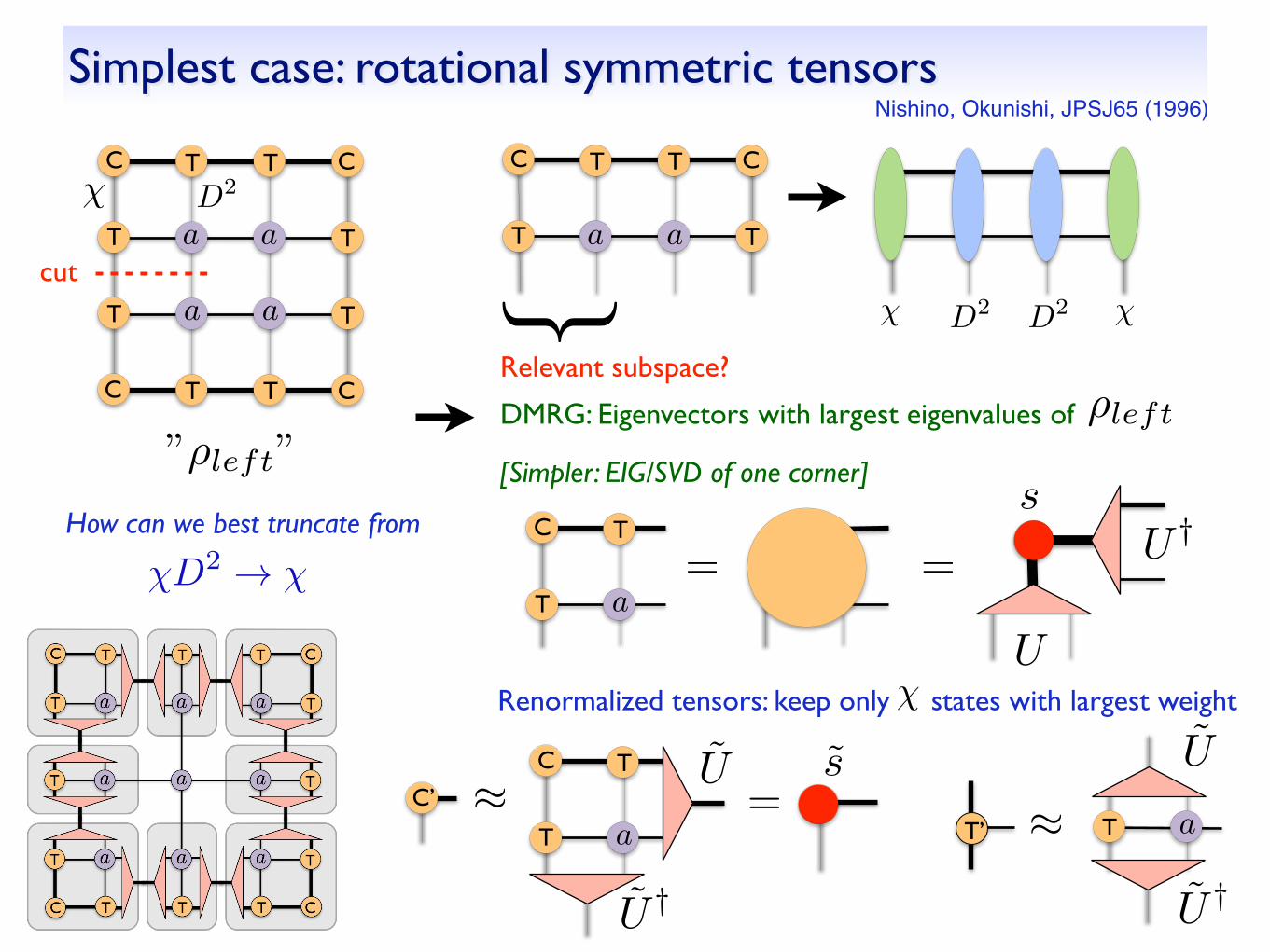
Simplest case: rotational symmetric tensors
C
C C
C
T
T
TT
T T
T
T
cut
”⇢left”
Nishino, Okunishi, JPSJ65 (1996)
a a
aa
Relevant subspace?
C C
T
T T
T
{
aa
�
DMRG: Eigenvectors with largest eigenvalues of ⇢left
D2 D2� �
How can we best truncate from
D2
�D2 ! �
[Simpler: EIG/SVD of one corner]
C T
T= =
a
U
sU †
�
C’ ⇡
Renormalized tensors: keep only states with largest weight
⇡T’ T a
U
U †
C T
T a
U †
U s<latexit sha1_base64="87p6218O+cGaTtO0I4cqfaOVrVE=">AAAB73icbVBNS8NAEJ3Ur1q/qh69LBbBU0lE0GPRi8cK9gPaUDabSbt0s4m7G6GE/gkvHhTx6t/x5r9x2+agrQ8GHu/NMDMvSAXXxnW/ndLa+sbmVnm7srO7t39QPTxq6yRTDFssEYnqBlSj4BJbhhuB3VQhjQOBnWB8O/M7T6g0T+SDmaTox3QoecQZNVbq9g0XIRI9qNbcujsHWSVeQWpQoDmofvXDhGUxSsME1brnuanxc6oMZwKnlX6mMaVsTIfYs1TSGLWfz++dkjOrhCRKlC1pyFz9PZHTWOtJHNjOmJqRXvZm4n9eLzPRtZ9zmWYGJVssijJBTEJmz5OQK2RGTCyhTHF7K2EjqigzNqKKDcFbfnmVtC/qnlv37i9rjZsijjKcwCmcgwdX0IA7aEILGAh4hld4cx6dF+fd+Vi0lpxi5hj+wPn8Acudj8s=</latexit><latexit sha1_base64="87p6218O+cGaTtO0I4cqfaOVrVE=">AAAB73icbVBNS8NAEJ3Ur1q/qh69LBbBU0lE0GPRi8cK9gPaUDabSbt0s4m7G6GE/gkvHhTx6t/x5r9x2+agrQ8GHu/NMDMvSAXXxnW/ndLa+sbmVnm7srO7t39QPTxq6yRTDFssEYnqBlSj4BJbhhuB3VQhjQOBnWB8O/M7T6g0T+SDmaTox3QoecQZNVbq9g0XIRI9qNbcujsHWSVeQWpQoDmofvXDhGUxSsME1brnuanxc6oMZwKnlX6mMaVsTIfYs1TSGLWfz++dkjOrhCRKlC1pyFz9PZHTWOtJHNjOmJqRXvZm4n9eLzPRtZ9zmWYGJVssijJBTEJmz5OQK2RGTCyhTHF7K2EjqigzNqKKDcFbfnmVtC/qnlv37i9rjZsijjKcwCmcgwdX0IA7aEILGAh4hld4cx6dF+fd+Vi0lpxi5hj+wPn8Acudj8s=</latexit><latexit sha1_base64="87p6218O+cGaTtO0I4cqfaOVrVE=">AAAB73icbVBNS8NAEJ3Ur1q/qh69LBbBU0lE0GPRi8cK9gPaUDabSbt0s4m7G6GE/gkvHhTx6t/x5r9x2+agrQ8GHu/NMDMvSAXXxnW/ndLa+sbmVnm7srO7t39QPTxq6yRTDFssEYnqBlSj4BJbhhuB3VQhjQOBnWB8O/M7T6g0T+SDmaTox3QoecQZNVbq9g0XIRI9qNbcujsHWSVeQWpQoDmofvXDhGUxSsME1brnuanxc6oMZwKnlX6mMaVsTIfYs1TSGLWfz++dkjOrhCRKlC1pyFz9PZHTWOtJHNjOmJqRXvZm4n9eLzPRtZ9zmWYGJVssijJBTEJmz5OQK2RGTCyhTHF7K2EjqigzNqKKDcFbfnmVtC/qnlv37i9rjZsijjKcwCmcgwdX0IA7aEILGAh4hld4cx6dF+fd+Vi0lpxi5hj+wPn8Acudj8s=</latexit><latexit sha1_base64="87p6218O+cGaTtO0I4cqfaOVrVE=">AAAB73icbVBNS8NAEJ3Ur1q/qh69LBbBU0lE0GPRi8cK9gPaUDabSbt0s4m7G6GE/gkvHhTx6t/x5r9x2+agrQ8GHu/NMDMvSAXXxnW/ndLa+sbmVnm7srO7t39QPTxq6yRTDFssEYnqBlSj4BJbhhuB3VQhjQOBnWB8O/M7T6g0T+SDmaTox3QoecQZNVbq9g0XIRI9qNbcujsHWSVeQWpQoDmofvXDhGUxSsME1brnuanxc6oMZwKnlX6mMaVsTIfYs1TSGLWfz++dkjOrhCRKlC1pyFz9PZHTWOtJHNjOmJqRXvZm4n9eLzPRtZ9zmWYGJVssijJBTEJmz5OQK2RGTCyhTHF7K2EjqigzNqKKDcFbfnmVtC/qnlv37i9rjZsijjKcwCmcgwdX0IA7aEILGAh4hld4cx6dF+fd+Vi0lpxi5hj+wPn8Acudj8s=</latexit>
=

General case: Renormalization step (left move)
R
U
V †
sR
€
≈SVD$
R−1
R−1 V
U †
s−1
€
≈
cut ! cut !
T1 C2C1 T1
a T2T4 a
a T2T4 a
T3 C3C4 T3
€
= QRupper half!
€
= Qlower half! R
QR#
QR#
C1 '
€
=C1 T1
P
€
=T4 'T4 a
P
P
€
=C4 'C4 T3
P
R
R
R−1
R−1
identity
R
R
V
U †
s−1/2
s−1/2
€
≈
approx. identity
P
P
=
=
projectors onto relevant subspace
Wang, Pižorn & Verstraete, PRB 83 (2011) Huang, Chen & Kao, PRB 86 (2012)PC, Rice, Troyer, PRL 113 (2014)T. Okubo, private comm.
alternatively: only use upper left and lower left corners
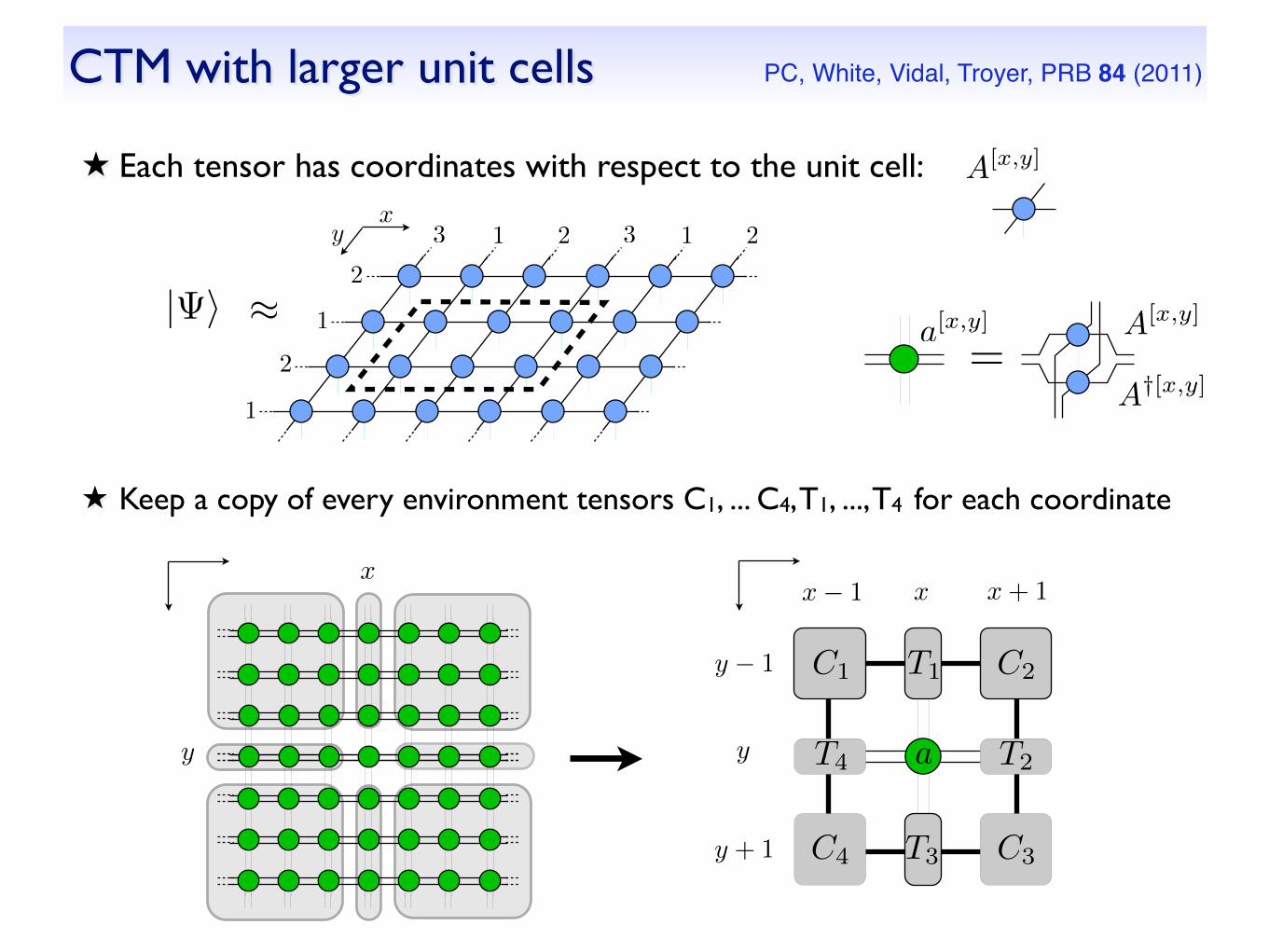
CTM with larger unit cells PC, White, Vidal, Troyer, PRB 84 (2011)
★ Each tensor has coordinates with respect to the unit cell: A[x,y]
xy 1 2 3 1 23
1
2
1
2
| i ⇡=
A[x,y]
A†[x,y]
a[x,y]
★ Keep a copy of every environment tensors C1, ... C4, T1, ..., T4 for each coordinate
C1 C2
C3C4
T1
T2
T3
T4 a
xx� 1 x+ 1
y
y + 1
y � 1
x
y

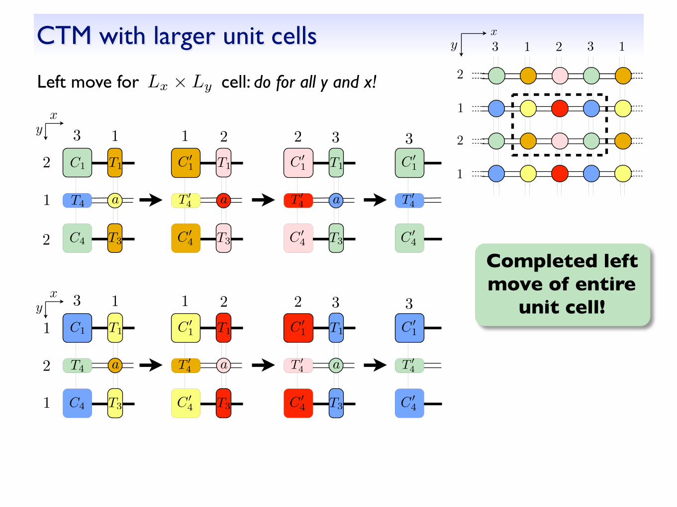
CTM with larger unit cells
Left move for cell: do for all x and y! Lx ⇥ Ly
=C 0[x,y]1
T [x,y]1
P [x�1,y]
C [x�1,y]1
C 0[x,y]4 =
T [x�1,y]3C [x�1,y]
4
P [x�1,y�1]
=
P [x�1,y]
a[x,y]
P [x�1,y�1]
T 0[x,y]4
T [x�1,y]4
• Do for all x 2 [1, Lx]
– Do for all y 2 [1, Ly]
⇤ Compute projectors P [x�1,y], P [x�1,y]
– Do for all y 2 [1, Ly]
⇤ Compute updated environment
tensors: C 0[x,y]1 , C 0[x,y]
4 , T 0[x,y]4
C1
C4
T1
T3
T4 a
xx� 1 xx� 1
C1 · T1
T4 · a
C4 · T3
C 01
T 04
C 04
x
y
y � 1
y + 1
xy
2
C 01
T 04
C 04
CTM with larger unit cells
Left move for cell: do for all y and x! Lx ⇥ Ly
1 2 33 1x
1
2
2
1C1
C4
T4
2
3
1
2
xy
y
C1
C4
T4
3
1
2
1
C 01
T 04
C 04
1
C 01
T 04
C 04
1
2
C 01
T 04
C 04
C 01
T 04
C 04
3
C 01
T 04
C 04
3
Completed left move of entire
unit cell!
T1
T3
a
1
T1
T3
a
1
2
T1
T3
a
2
T1
T3
a
3
T1
T3
a
3
T1
T3
a
xy
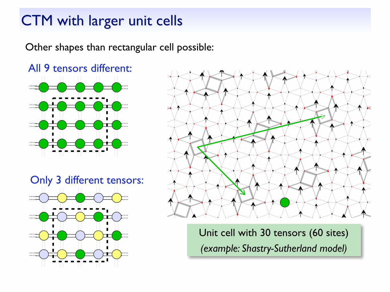
CTM with larger unit cells
Other shapes than rectangular cell possible:
All 9 tensors different:
Only 3 different tensors:
Unit cell with 30 tensors (60 sites)
(example: Shastry-Sutherland model)

Contracting the PEPS/iPEPS using TRG Gu, Levin, Wen, B78, (2008)Levin, Nave, PRL99 (2007)Xie et al. PRL 103, (2009)
★ Contract PEPS with periodic boundary conditions★ Finite or infinite systems★ Related schemes: SRG, HOTRG, HOSRG, ...
Tensor Renormalization Group
SVD dimension �sublattice A:
SVDsublattice B:

More advanced: Tensor network renormalization
★ Additional ingredient: Disentanglers★ Remove short-range entanglement at each
coarse-graining step (key idea of the MERA) ★ Faster convergence with chi★ Especially important for critical systems★ Another variant: Loop-TNR:
Yang, Gu & Wen, PRL 118 (2017)
Evenbly & Vidal, PRL 115 (2015)
Contracting the PEPS★ Exact contraction of an PEPS is exponentially hard!
use controlled approximate contraction scheme
MPS-MPO-based approaches
Corner transfer matrix method
TRG Tensor Renormalization Group(variants: HOTRG, SRG, HOSRG)
Murg,Verstraete,Cirac, PRA75 ’07Jordan,et al. PRL79 (2008)Haegeman & Verstraete (2017)…
Nishino, Okunishi, JPSJ65 (1996)Orus, Vidal, PRB 80 (2009)Fishman et al, PRB 98 (2018)…
Levin, Nave, PRL99 (2007)Xie et al. PRL 103 (2009)Xie et al. PRB 86 (2012), …
★Accuracy of the approximate contraction is controlled by “boundary dimension” �
★Convergence in needs to be carefully checked�
★Overall cost: with � ⇠ D2O(D10...14)
TNRTensor Network Renormalization
Loop-TNR: Yang, Gu & Wen, PRL 118 (2017)
Evenbly & Vidal, PRL 115 (2015)

MPS
Structure Variational
ansatz
iterative optimization of individual tensors
(energy minimization)imaginary time
evolution
Contraction of the tensor network
exact / approximate
Find the best (ground) state
|��
Compute observables��|O|�⇥
PEPS2D MERA
1D MERA
✓
✓
Summary: Tensor network algorithm for ground state

Optimization
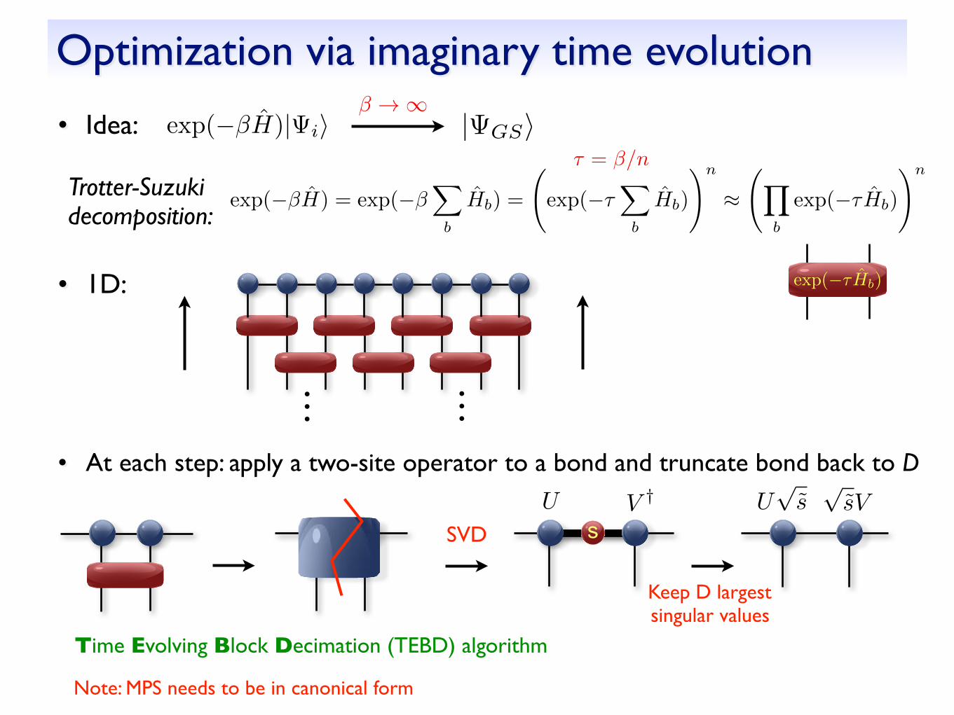
Optimization via imaginary time evolution
• Idea:
exp(�⌧Hb)
• At each step: apply a two-site operator to a bond and truncate bond back to D
Keep D largest singular values
Ups
psV
SVD sU V †
Time Evolving Block Decimation (TEBD) algorithm
Note: MPS needs to be in canonical form
...
...
exp(��H)| ii� ! 1
| GSi⌧ = �/n
exp(��H) = exp(��
X
b
Hb) =
exp(�⌧
X
b
Hb)
!n
⇡ Y
b
exp(�⌧Hb)
!n
Trotter-Suzukidecomposition:
• 1D:
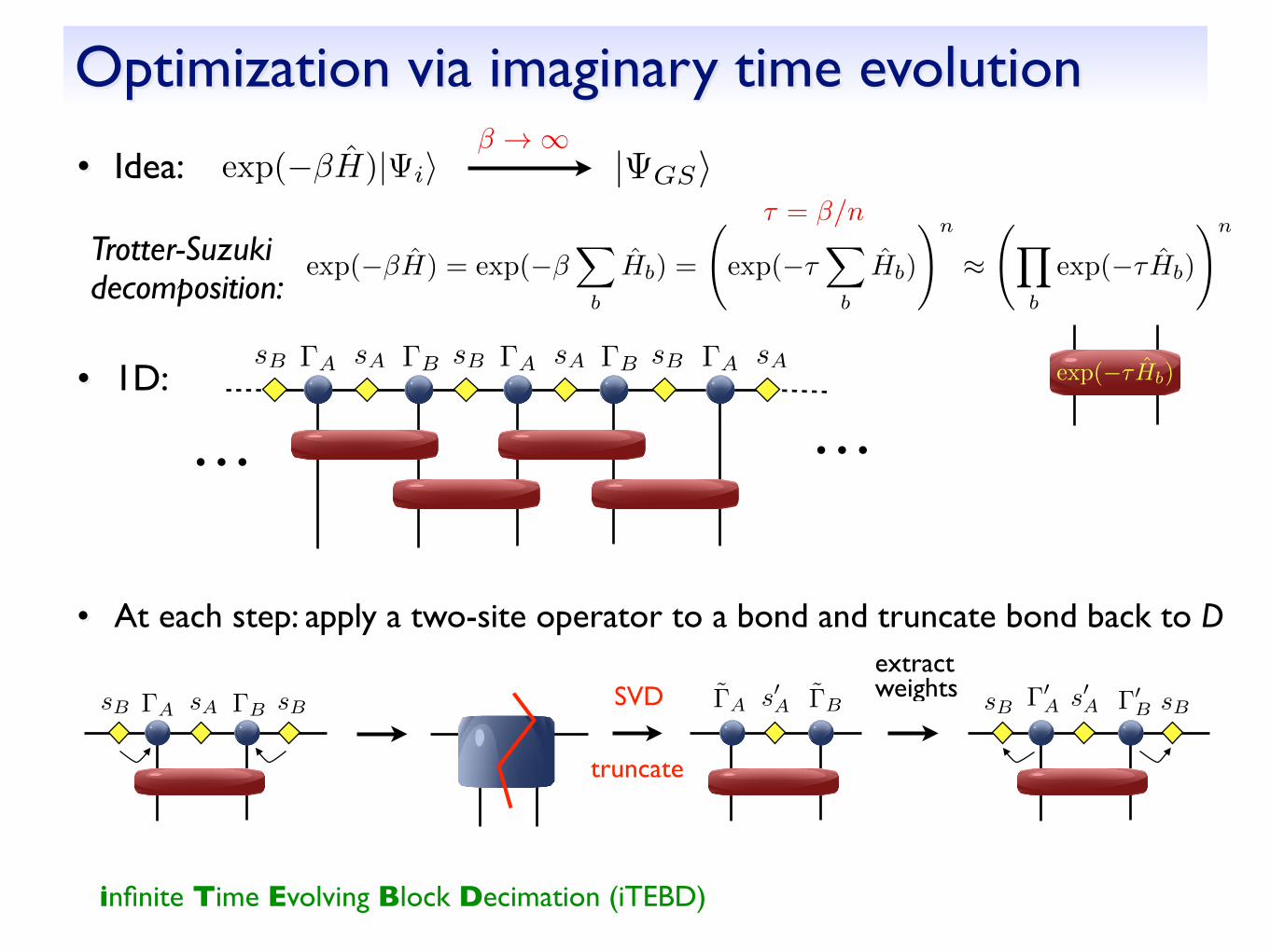
Optimization via imaginary time evolution
• Idea:
exp(�⌧Hb)
• At each step: apply a two-site operator to a bond and truncate bond back to D
infinite Time Evolving Block Decimation (iTEBD)
exp(��H)| ii� ! 1
| GSi⌧ = �/n
exp(��H) = exp(��
X
b
Hb) =
exp(�⌧
X
b
Hb)
!n
⇡ Y
b
exp(�⌧Hb)
!n
Trotter-Suzukidecomposition:
• 1D: �A �BsA sB �A sAsB �B sB
......
�A sA
SVD�A �BsA sBsB sBsB�A �B
extract weights �0
B�0A
truncate
s0A s0A

Optimization via imaginary time evolution
Cluster update Wang, Verstraete, arXiv:1110.4362 (2011)
• 2D: same idea: apply to a bond and truncate bond back to D
exp(�⌧Hb)
• However, SVD update is not optimal (because of loops in PEPS)!
simple update (SVD)
★ “local” update like in TEBD
★ Cheap, but not optimal (e.g. overestimates magnetization in S=1/2 Heisenberg model)
Jiang et al, PRL 101 (2008)full update
★ Take the full wave function into account for truncation
★ optimal, but computationally more expensive
★ Fast-full update [Phien et al, PRB 92 (2015)]
Jordan et al, PRL 101 (2008)
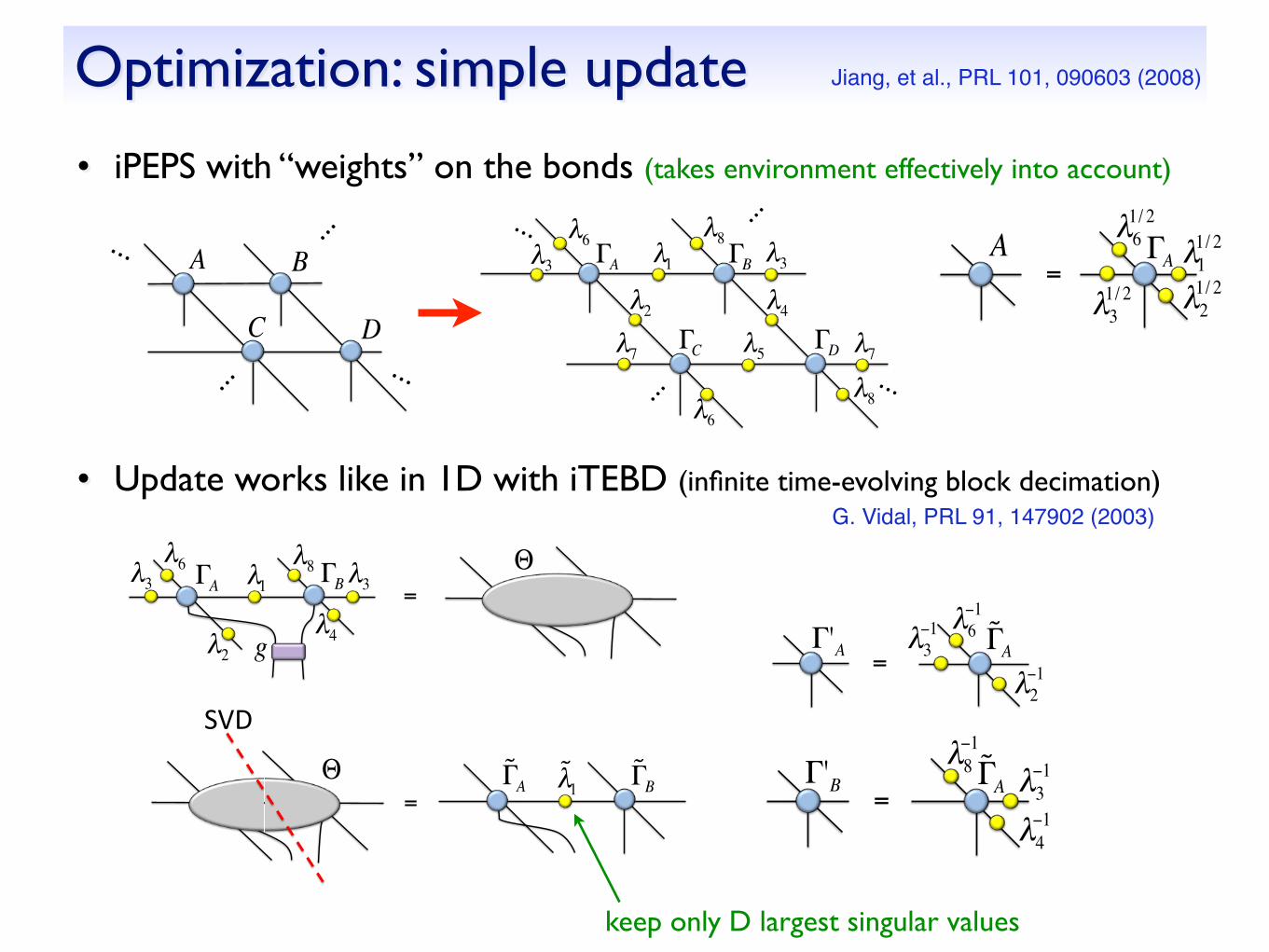
Optimization: simple update
• iPEPS with “weights” on the bonds (takes environment effectively into account)
€
A
€
B
€
C
€
D
..."
..."
..."
..." €
λ1
€
λ2
€
λ5
€
λ4
€
λ3
€
λ3
€
λ6
€
λ6
€
λ8
€
λ8
€
λ7
€
λ7
..."
..."
..."
..."
€
ΓA
€
ΓB
€
ΓC
€
ΓD€
λ61/ 2
€
λ11/ 2
€
λ21/ 2
€
λ31/ 2
€
=
€
A
€
ΓA
keep only D largest singular values€
˜ Γ A
€
˜ λ 1
€
=
€
Θ
SVD$
€
˜ Γ B€
λ6−1
€
λ3−1
€
λ2−1
€
=
€
Γ'A
€
˜ Γ A
€
λ8−1
€
λ3−1
€
λ4−1
€
=
€
Γ'B
€
˜ Γ A
Jiang, et al., PRL 101, 090603 (2008)
• Update works like in 1D with iTEBD (infinite time-evolving block decimation)
€
g
€
λ1
€
λ6
€
λ3
€
λ2€
λ8
€
λ4
€
λ3
€
Θ
€
=
€
ΓA
€
ΓB
G. Vidal, PRL 91, 147902 (2003)

Trick to make it cheaper
• Idea: Split off the part of the tensor which is updated
€
g
€
λ1
€
λ6
€
λ3
€
λ2€
λ8
€
λ4
€
λ3
€
ΓA
€
ΓB
€
=
€
g€
=U sVT
€
=
€
g
SVD$
€
=
€
λ6−1
€
λ3−1
€
λ2−1
€
=
€
Γ'A
€
˜ Γ A
€
λ8−1
€
λ3−1
€
λ4−1
€
=
€
Γ'B
€
˜ Γ B€
g
€
=
€
˜ Γ A
€
˜ λ 1
€
˜ Γ B
keep only D largest singular values
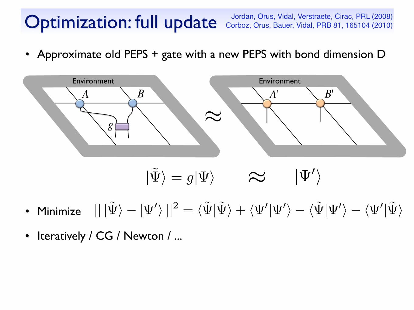
Optimization: full update
• Approximate old PEPS + gate with a new PEPS with bond dimension D
€
g€
A
€
BEnvironment
| i = g| i
Environment
€
A'
€
B'
⇡
| 0i⇡
Jordan, Orus, Vidal, Verstraete, Cirac, PRL (2008)Corboz, Orus, Bauer, Vidal, PRB 81, 165104 (2010)
• Minimize
• Iteratively / CG / Newton / ...
|| | i � | 0i ||2 = h | i+ h 0| 0i � h | 0i � h 0| i

Full-update: details
• Split off the part of the tensor which is updated
€
=X pA
€
=YqB
=Environmentof p and q tensors
U (sV)
d(p0, q0) = h | i+ h 0| 0i � h | 0i � h 0| i“Cost-function”
+ - -
qp qpp0 q0 p0 q0
g g
p† q†
g†
qp
p† q†
⇡ find new p’, and q’ to minimize: || | i � | 0i ||| i = g| (p, q)i | 0(p0, q0)i2
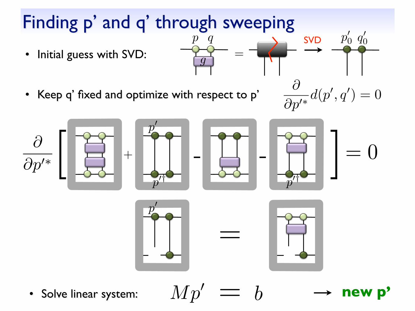
Finding p’ and q’ through sweeping
• Initial guess with SVD: =
p00 q00qp
• Keep q’ fixed and optimize with respect to p’ @
@p0⇤d(p0, q0) = 0
Mp0 b=• Solve linear system: new p’
SVD
= 0[ [@
@p0⇤+ - -
p0† p0†
p0
=p0
g
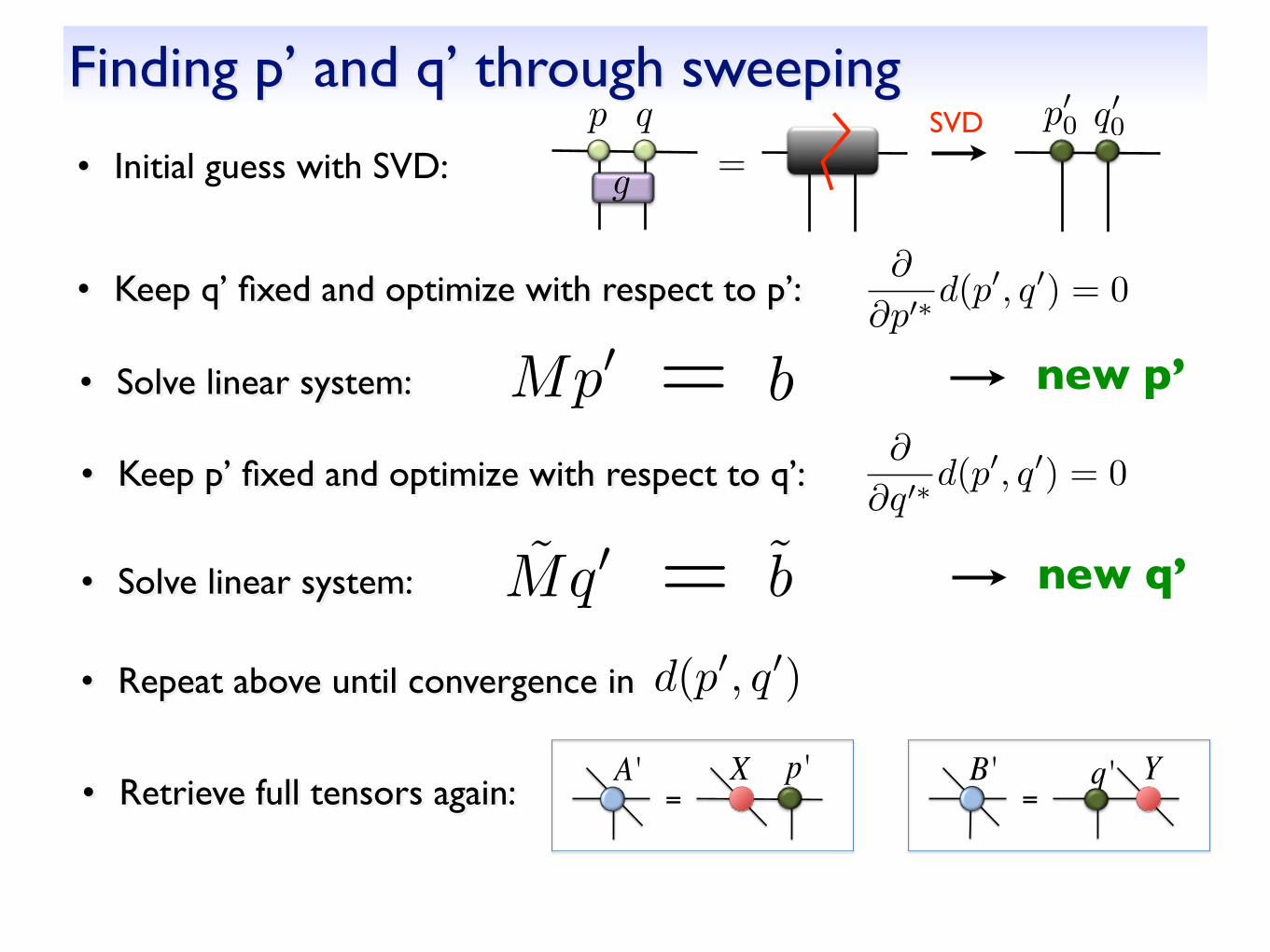
Finding p’ and q’ through sweeping
• Initial guess with SVD: =
p00 q00qp
• Keep q’ fixed and optimize with respect to p’: @
@p0⇤d(p0, q0) = 0
Mp0 b=• Solve linear system: new p’
• Keep p’ fixed and optimize with respect to q’: @
@q0⇤d(p0, q0) = 0
=• Solve linear system: new q’Mq0 b
• Repeat above until convergence in d(p0, q0)
SVD
g
• Retrieve full tensors again:
€
=X p 'A '
€
=Yq 'B '
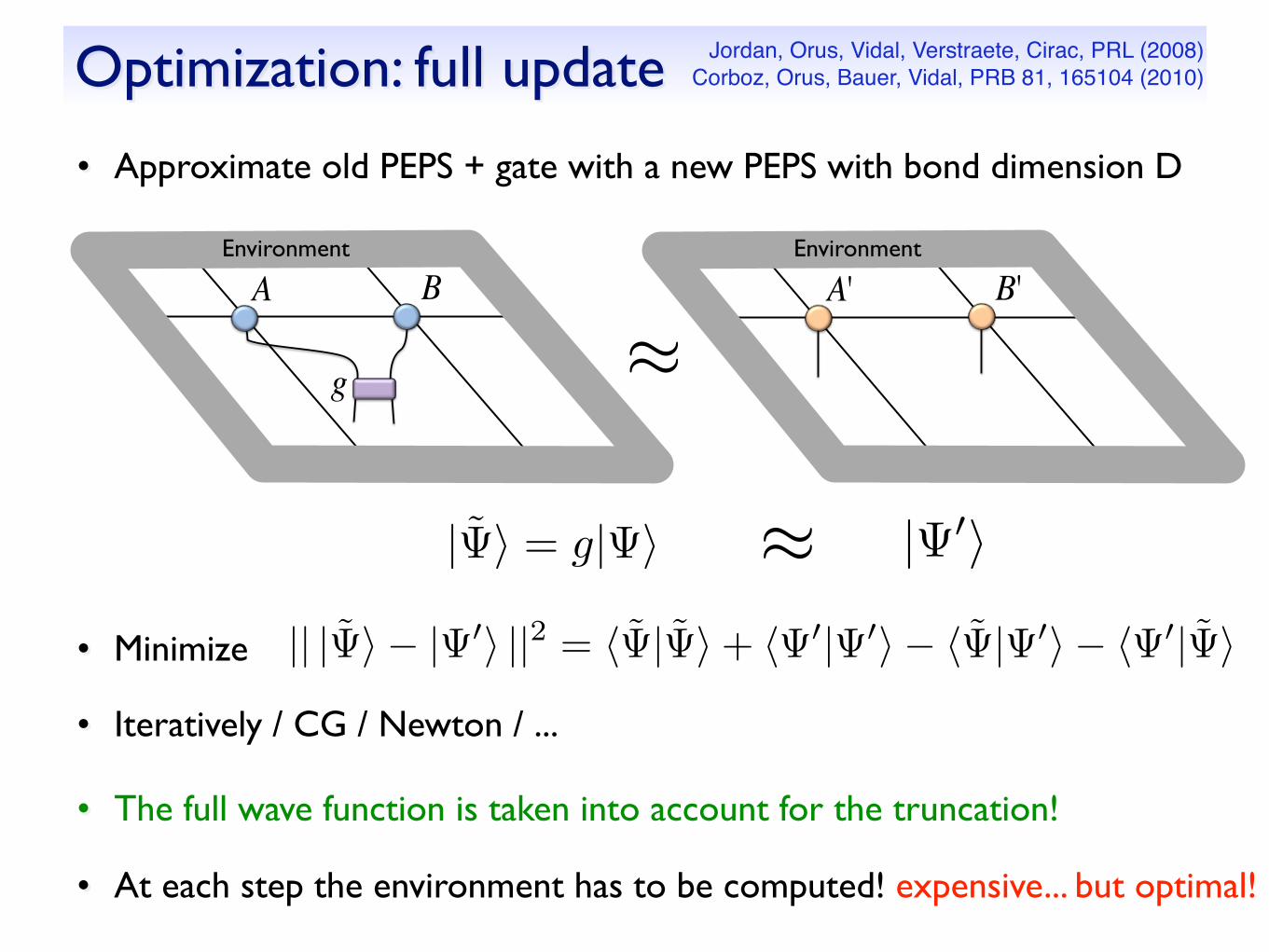
Optimization: full update
• Approximate old PEPS + gate with a new PEPS with bond dimension D
€
g€
A
€
BEnvironment
| i = g| i
Environment
€
A'
€
B'
⇡
| 0i⇡
• The full wave function is taken into account for the truncation!
• At each step the environment has to be computed! expensive... but optimal!
Jordan, Orus, Vidal, Verstraete, Cirac, PRL (2008)Corboz, Orus, Bauer, Vidal, PRB 81, 165104 (2010)
• Minimize
• Iteratively / CG / Newton / ...
|| | i � | 0i ||2 = h | i+ h 0| 0i � h | 0i � h 0| i

Optimization: simple vs full update
simple update ★ “local” update like in TEBD
★ Cheap, but not optimal (e.g. overestimates magnetization in S=1/2 Heisenberg model)
full update ★ Take the full wave function into
account for truncation
★ optimal, but computationally more expensive
0 0.1 0.2 0.3 0.4 0.50.3
0.32
0.34
0.36
0.38
0.4
0.42
1/Dm
[%]
Simple updateFull update
exact result
Example: 2D Heisenberg model
• Combine the two: Use simple update to get an initial state for the full update
• Don’t compute environment from scratch but recycle previous one fast full update Phien, Bengua, Tuan, PC, Orus, PRB 92 (2015)
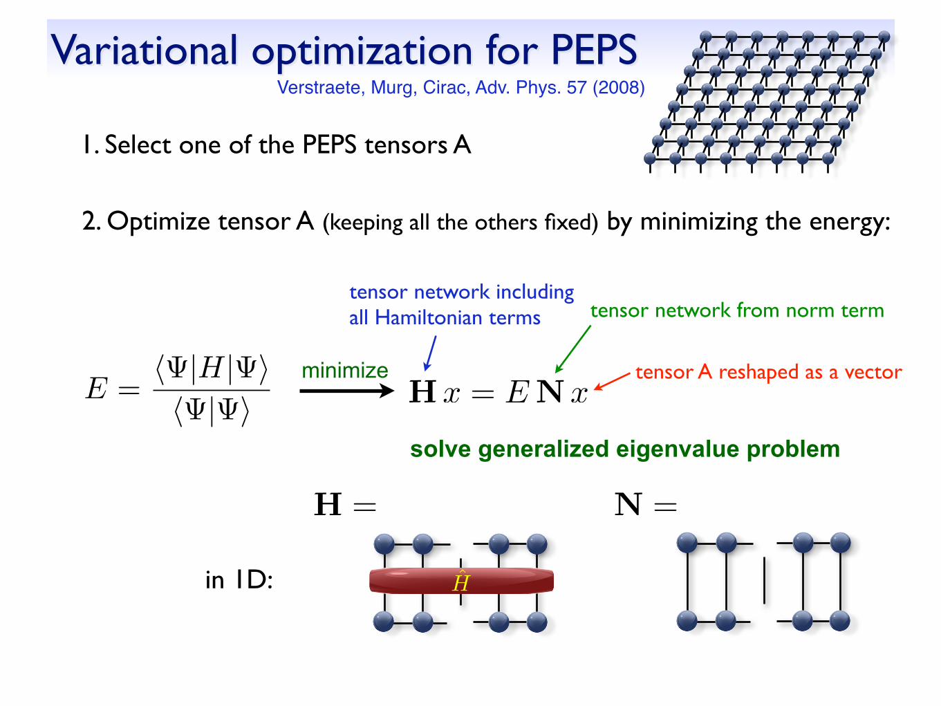
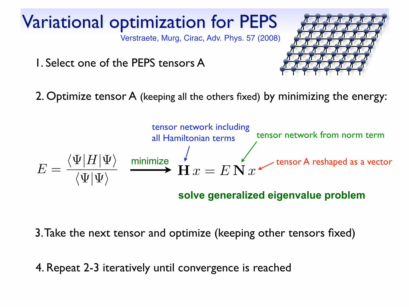
1. Select one of the PEPS tensors A
Variational optimization for PEPS
E =h |H| ih | i
tensor A reshaped as a vector
tensor network including all Hamiltonian terms tensor network from norm term
2. Optimize tensor A (keeping all the others fixed) by minimizing the energy:
Hx = ENx
solve generalized eigenvalue problem
minimize
Verstraete, Murg, Cirac, Adv. Phys. 57 (2008)
in 1D: H
H = N =
1. Select one of the PEPS tensors A
Variational optimization for PEPS
E =h |H| ih | i
tensor A reshaped as a vector
tensor network including all Hamiltonian terms tensor network from norm term
2. Optimize tensor A (keeping all the others fixed) by minimizing the energy:
Hx = ENx
solve generalized eigenvalue problem
minimize
Verstraete, Murg, Cirac, Adv. Phys. 57 (2008)
3. Take the next tensor and optimize (keeping other tensors fixed)
4. Repeat 2-3 iteratively until convergence is reached
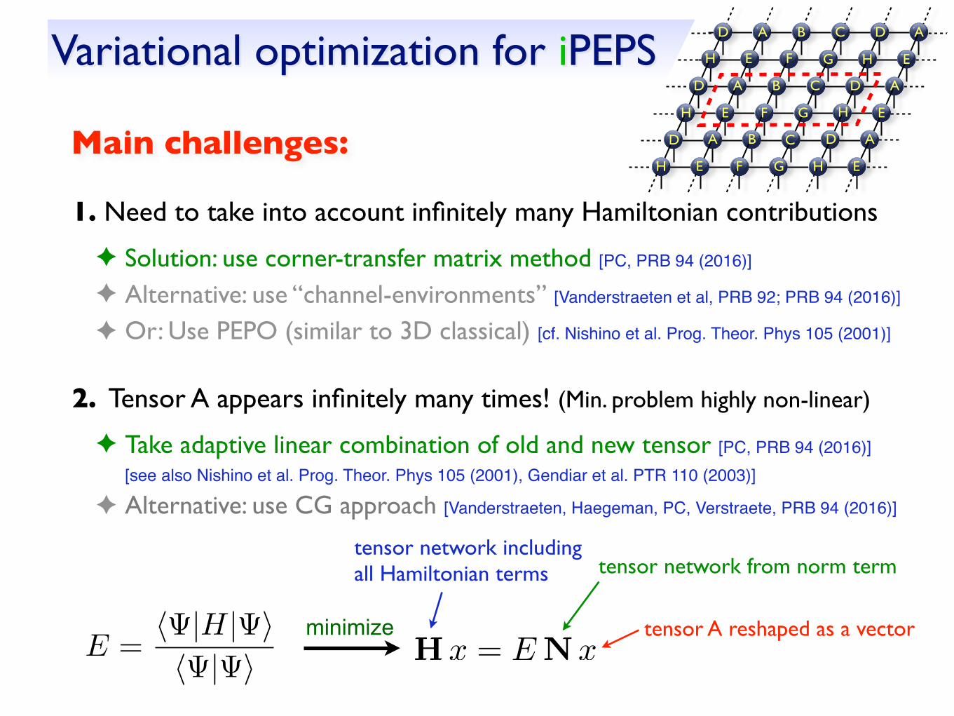
Variational optimization for iPEPS
E =h |H| ih | i
tensor A reshaped as a vector
tensor network including all Hamiltonian terms tensor network from norm term
Hx = ENxminimize
B C
F G
D A
H
D A
H E
B C
F G
D A
H E
D A
H E
B C
F G
D A
H E
D A
H E
E
| i ⇡u
d
l r
pA
(a) MPS
(b) iPEPS
A
i1
B
i2
C
i3
D
i4
E
i5
F
i6
j1 j2 j3 j4 j5
i1 i2 i3 i4 i5 i6
ci1i2i3i4i5i6 ⇡
Aldrup
Cj2j3i3
Main challenges:
1. Need to take into account infinitely many Hamiltonian contributions
✦ Solution: use corner-transfer matrix method [PC, PRB 94 (2016)] ✦ Alternative: use “channel-environments” [Vanderstraeten et al, PRB 92; PRB 94 (2016)]
✦ Or: Use PEPO (similar to 3D classical) [cf. Nishino et al. Prog. Theor. Phys 105 (2001)]
2. Tensor A appears infinitely many times! (Min. problem highly non-linear)
✦ Take adaptive linear combination of old and new tensor [PC, PRB 94 (2016)] [see also Nishino et al. Prog. Theor. Phys 105 (2001), Gendiar et al. PTR 110 (2003)]
✦ Alternative: use CG approach [Vanderstraeten, Haegeman, PC, Verstraete, PRB 94 (2016)]
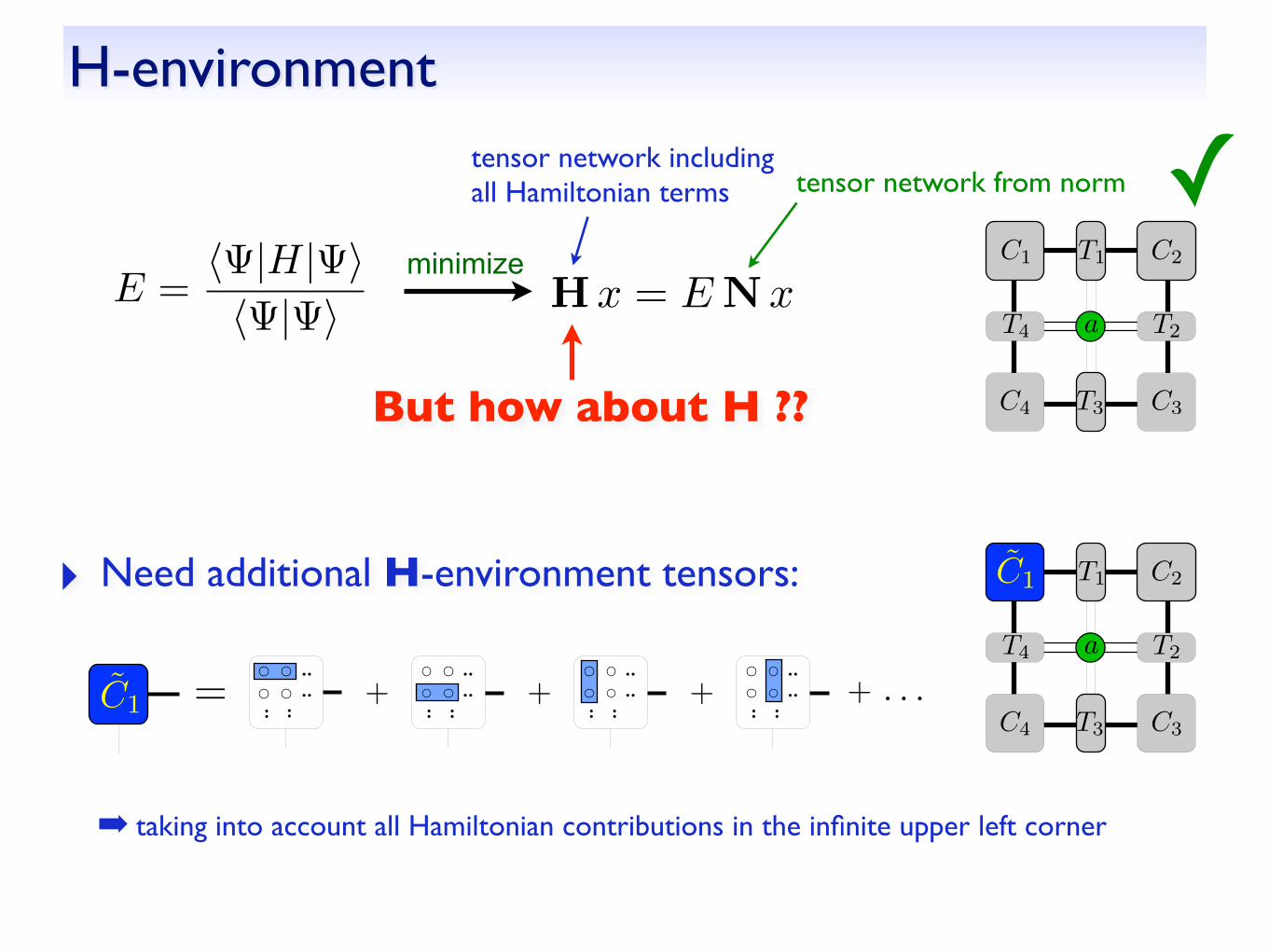
H-environment
E =h |H| ih | i
tensor network including all Hamiltonian terms tensor network from norm
Hx = ENxminimize
✓ .C1 C2
C3C4
T1
T2
T3
T4 a
‣ Need additional H-environment tensors: C2
C3C4
T1
T2
T3
T4 a
C1
..
..
.. ..
+ . . .....
.. ..
..
..
.. ..
..
..
.. ..
+++=C1
➡ taking into account all Hamiltonian contributions in the infinite upper left corner
But how about H ??
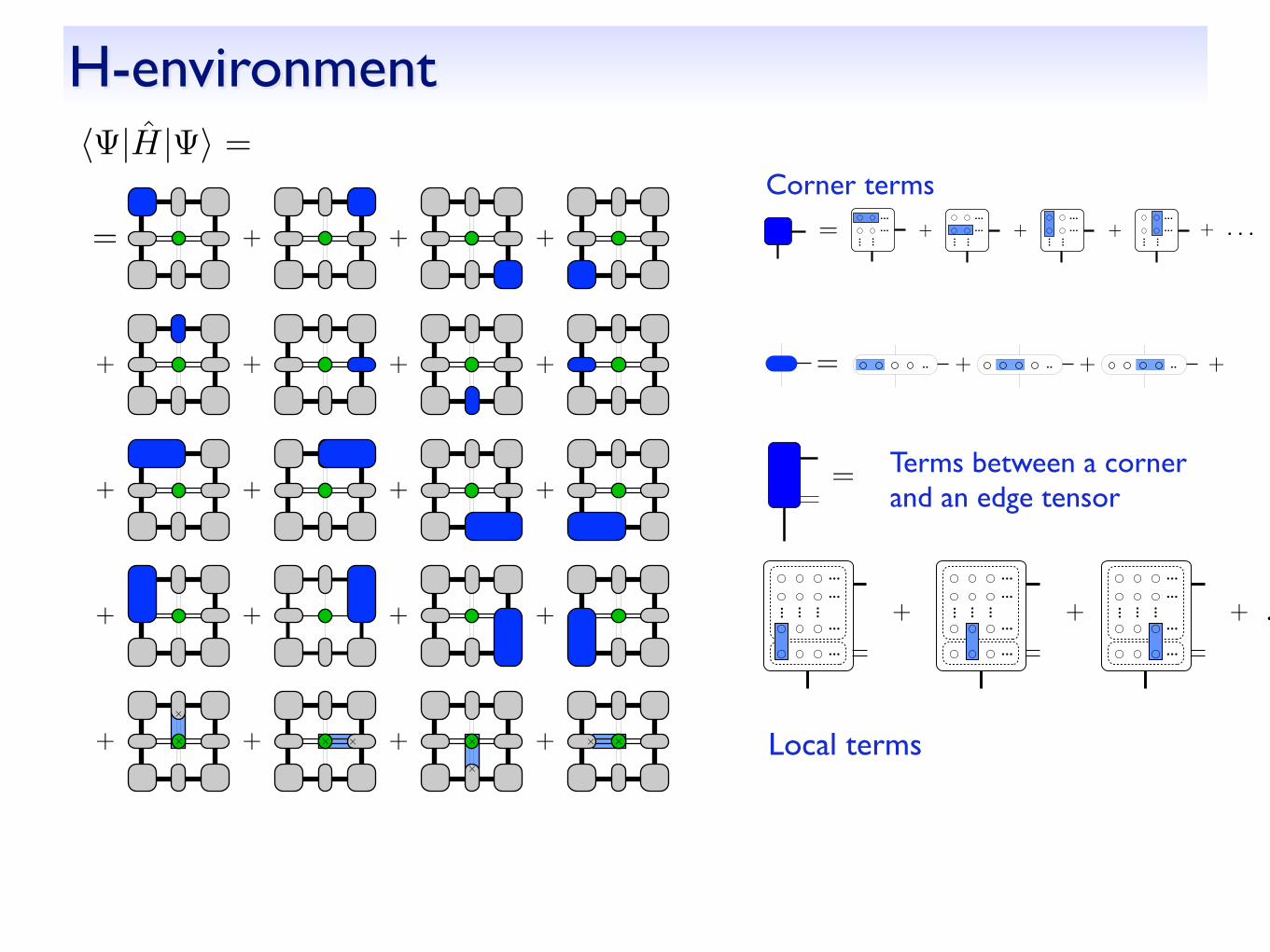
H-environment
+ + +
+ + ++
+ + ++
+ + ++
+ + ++
=
h |H| i =
+
+
+
+
++++
= .. ..+ ..+ +
+ + +
+ + ++
+ + ++
+ + ++
+ + ++
=
h |H| i =
T4 = = ... ...+ ...+ + . . .
Cv1 =......
... ... ...
...
...
...
...
... ... ...
...
...
...
...
... ... ...
...
...
+ += + . . .
C1
...
...
... ...
+ . . .......
... ...
...
...
... ...
...
...
... ...
+++= =
+
+
+
+
++++
+ + +
+ + ++
+ + ++
+ + ++
+ + ++
=
h |H| i =
T4 = = ... ...+ ...+ + . . .
Cv1 =......
... ... ...
...
...
...
...
... ... ...
...
...
...
...
... ... ...
...
...
+ += + . . .
C1
...
...
... ...
+ . . .......
... ...
...
...
... ...
...
...
... ...
+++= =
++
+
+
++++
+ + +
+ + ++
+ + ++
+ + ++
+ + ++
=
h |H| i =
T4 = = ... ...+ ...+ + . . .
Cv1 =......
... ... ...
...
...
...
...
... ... ...
...
...
...
...
... ... ...
...
...
+ += + . . .
C1
...
...
... ...
+ . . .......
... ...
...
...
... ...
...
...
... ...
+++= =
+
+
+
+
++++
Local terms
Terms between a corner and an edge tensor
Corner terms
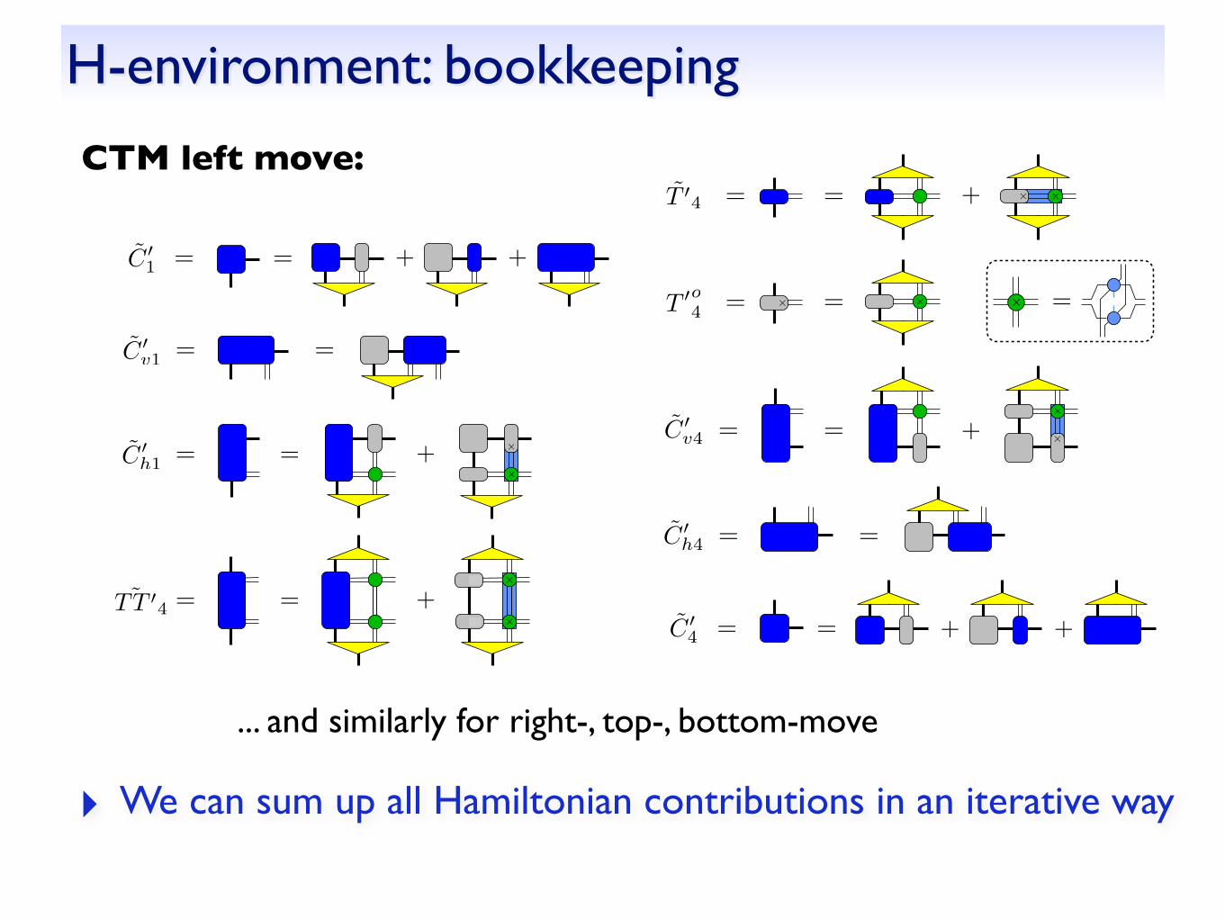
H-environment: bookkeeping
CTM left move:
= +
++
++
= +++
+ = +
= + +
=
= +
++
=
=
=
=
=
=
= + +
=
= ++
+
=
=
=
C 01
C 0v1
C 0h1
C 0h4
˜TT 04
T 04
C 0v4
C 04
T 0o4
=+
... and similarly for right-, top-, bottom-move
‣ We can sum up all Hamiltonian contributions in an iterative way
= +
++
++
= +++
+ = +
= + +
=
= +
++
=
=
=
=
=
=
= + +
=
= ++
+
=
=
=
C 01
C 0v1
C 0h1
C 0h4
˜TT 04
T 04
C 0v4
C 04
T 0o4
=+
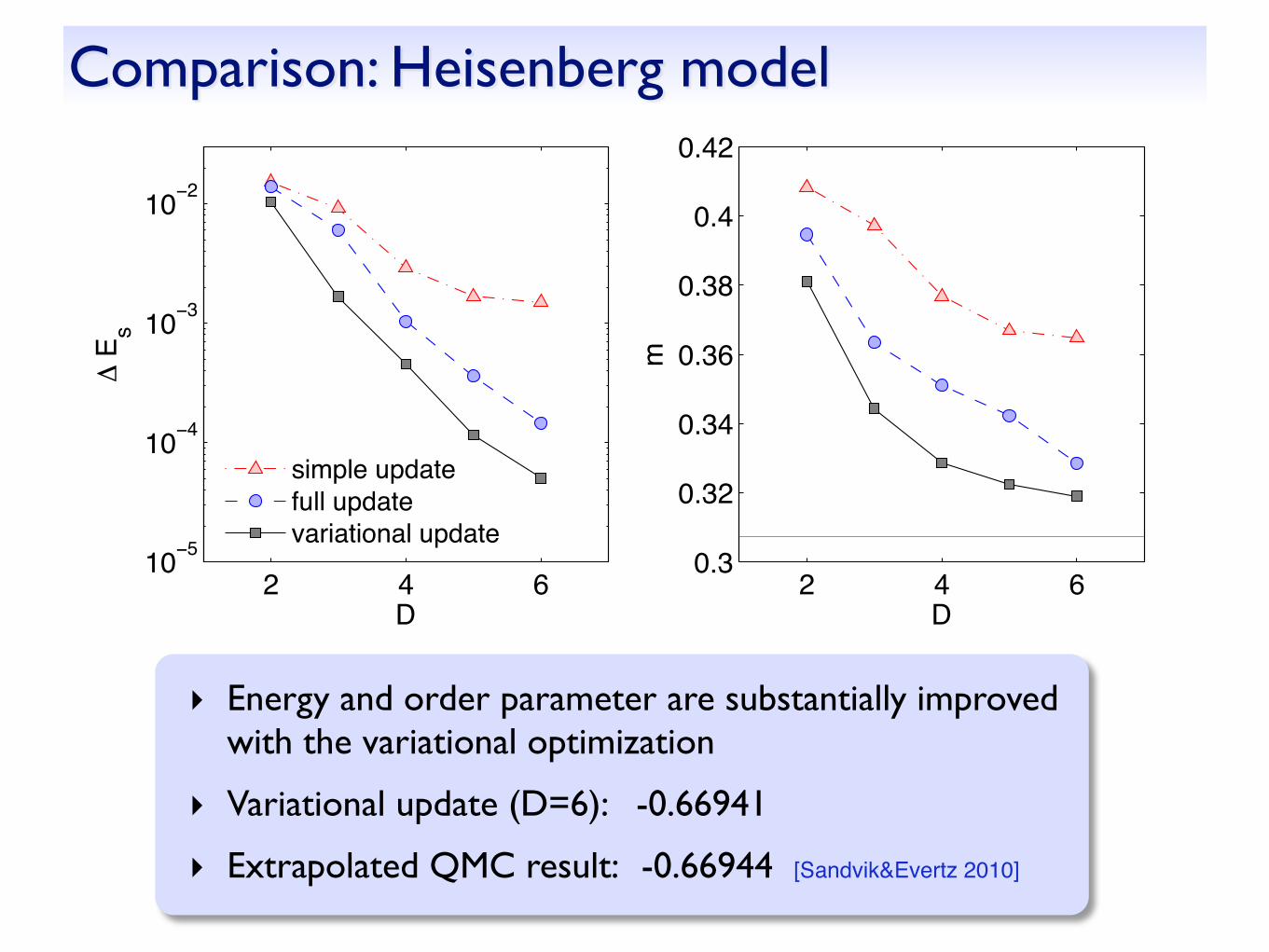
Comparison: Heisenberg model
2 4 610−5
10−4
10−3
10−2
D
Δ E
s
simple updatefull updatevariational update
2 4 60.3
0.32
0.34
0.36
0.38
0.4
0.42
Dm
0 200 400
−0.669
−0.6685
−0.668
−0.6675
seconds0 0.05 0.1 0.15
−0.669
−0.6688
−0.6686
−0.6684
τ
full updatevariatonal update
Es/JEs/J
‣ Energy and order parameter are substantially improved with the variational optimization
‣ Variational update (D=6): -0.66941
‣ Extrapolated QMC result: -0.66944 [Sandvik&Evertz 2010]
2 4 610−5
10−4
10−3
10−2
D
Δ E
s
simple updatefull updatevariational update
2 4 60.3
0.32
0.34
0.36
0.38
0.4
0.42
Dm
0 200 400
−0.669
−0.6685
−0.668
−0.6675
seconds0 0.05 0.1 0.15
−0.669
−0.6688
−0.6686
−0.6684
τ
full updatevariatonal update
Es/JEs/J
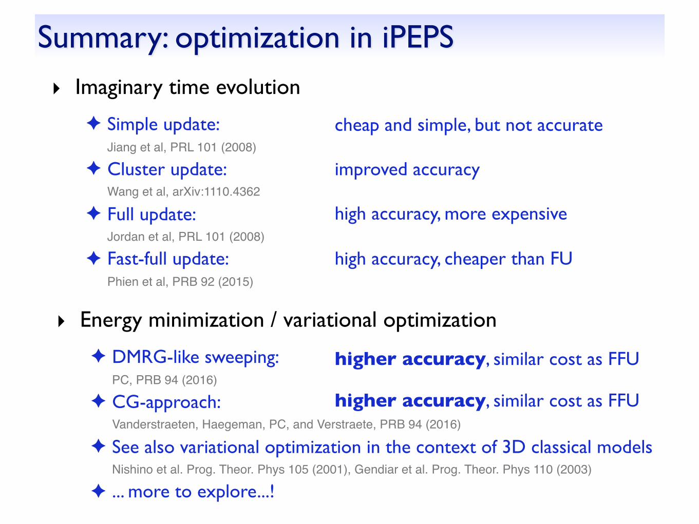
Summary: optimization in iPEPS
‣ Imaginary time evolution
✦ Simple update: Jiang et al, PRL 101 (2008)
✦ Cluster update: Wang et al, arXiv:1110.4362
✦ Full update: Jordan et al, PRL 101 (2008)
✦ Fast-full update: Phien et al, PRB 92 (2015)
cheap and simple, but not accurate
improved accuracy
high accuracy, more expensive
‣ Energy minimization / variational optimization
✦ DMRG-like sweeping: PC, PRB 94 (2016)
✦ CG-approach: Vanderstraeten, Haegeman, PC, and Verstraete, PRB 94 (2016)
✦ See also variational optimization in the context of 3D classical modelsNishino et al. Prog. Theor. Phys 105 (2001), Gendiar et al. Prog. Theor. Phys 110 (2003)
✦ ... more to explore...!
higher accuracy, similar cost as FFU
higher accuracy, similar cost as FFU
high accuracy, cheaper than FU
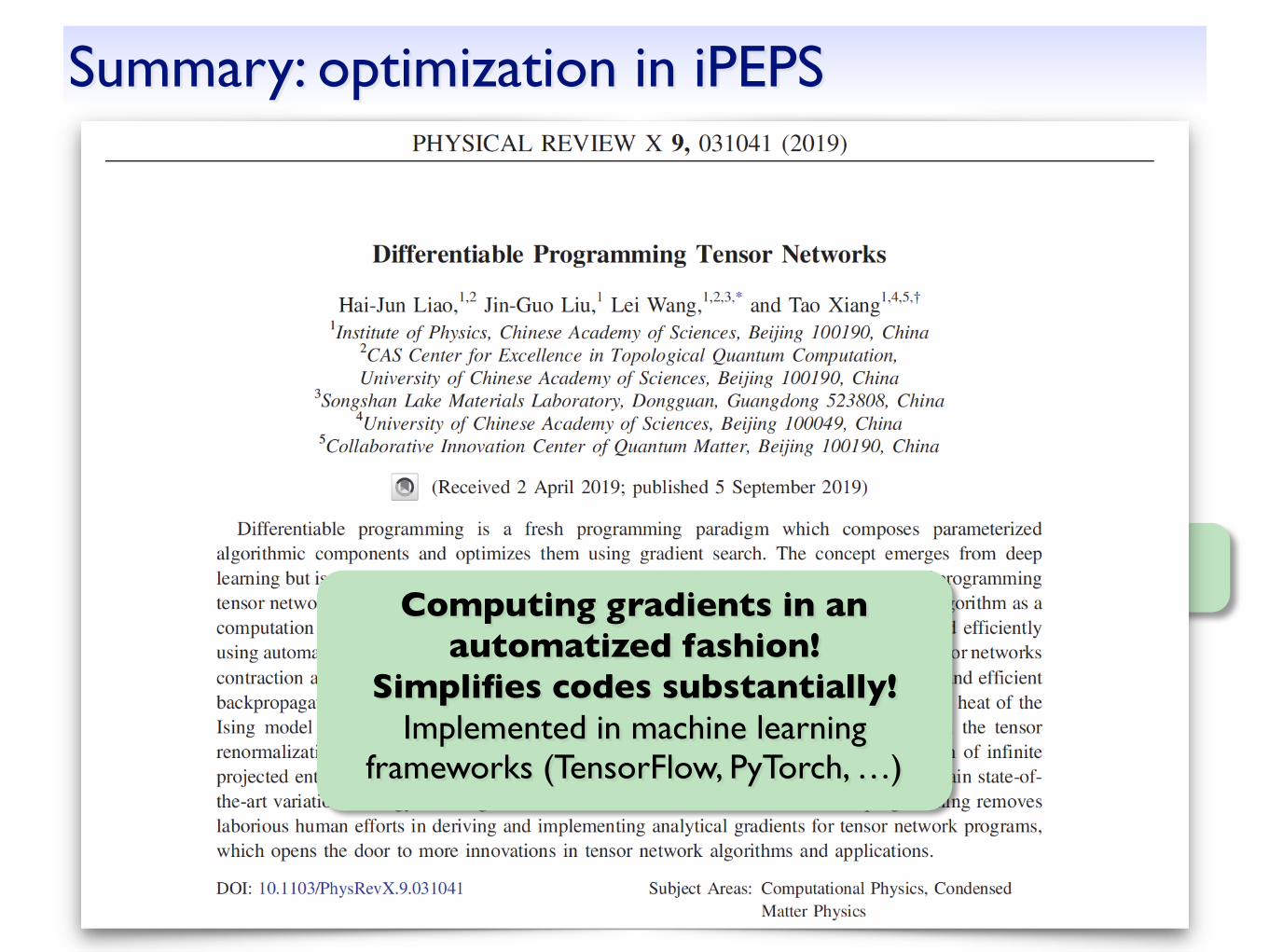
+ COMBINATIONS!Computing gradients in an
automatized fashion! Simplifies codes substantially!
Implemented in machine learning frameworks (TensorFlow, PyTorch, …)

Automatic differentiationLiao, Liu, Wang, Xiang, PRX (2019)
input (tensors)
computation graph:
output (e.g. energy)
Compute the gradient via chain rule:
from left to right (back propagation algorithm)
Define forward and backward function of each elementary operation (primitives), e.g. addition, multiplication, math functions, matrix-matrix multiplications, eigenvalue decompositions, etc.
→ Gradient can be computed in an automatized fashion
See Juraj Hasik’s talk on Thursday!
MPS
Structure Variational
ansatz
iterative optimization of individual tensors
(energy minimization)imaginary time
evolution
Contraction of the tensor network
exact / approximate
Find the best (ground) state
|��
Compute observables��|O|�⇥
PEPS2D MERA
1D MERA
✓
✓✓
Summary: Tensor network algorithms (ground state)