Sear h Heuristi s for Constraint-AidedEmbodiment DesignR. Chenouard a,∗, L. Granvilliers b P. Sébastian a

aENSAM Bordeaux, TRansferts E oulements FLuides Energétique, CNRS,F-33405, Talen e CedexbUniversity of Nantes, Laboratoire d'Informatique de Nantes Atlantique, CNRS,BP 92208, F-44322 Nantes Cedex 3

Preprint submitted to AIEDAM 3 De ember 2007

hal-0

0426

706,

ver

sion

1 -

23 M

ar 2

010

Author manuscript, published in "Artificial Intelligence for Engineering Design, Analysis and Manufacturing 23, 2 (2009) 175-195" DOI : 10.1017/S0890060409000055

Abstra tEmbodiment Design (ED) is an early phase of produ t development. ED prob-lems onsist of �nding solution prin iples that satisfy produ t requirements su has physi s behaviors and intera tions between omponents. Constraint satisfa tionte hniques are useful to solve onstraint-based models that are often partial, hetero-geneous, and un ertain in ED. In this paper, new onstraint satisfa tion te hniquesare proposed to ta kle pie ewise de�ned physi s phenomena or skill-based rules andmultiple ategories of variables arising in design appli ations. New sear h heuristi sand a global pie ewise onstraint are introdu ed in the bran h-and-prune framework.The apabilities of these te hniques are illustrated on both a ademi and real-worldproblems. The latter have omplete models presented in the appendix.Key words: sear h, heuristi , embodiment design, onstraint satisfa tion

∗ Corresponding author.Email addresses: raphael. henouard�bordeaux.ensam.fr (R. Chenouard),laurent.granvilliers�univ-nantes.fr (L. Granvilliers),patri k.sebastian�bordeaux.ensam.fr (P. Sébastian).2

hal-0

0426

706,

ver

sion

1 -

23 M

ar 2

010

1 Introdu tionThe design pro ess is a sequen e of phases from the de�nition of needs andrequirements to preliminary design and detailed design (Pahl & Beitz, 1996).Preliminary design in ludes on eptual design (CD) and embodiment design(ED). The ED phase investigates the feasibility of some produ t s hemes ob-tained from the CD phase. This phase mainly ta kles physi s behaviors andintera tions between the produ t, its omponents and environments. Produ tmodeling is based on the de�nition of the laws of physi s, fun tional models,e onomi riteria, et .In this paper we fo us on robust ED taking into a ount variability, un er-tainty or impre ision in the design pro ess. The goal is to determine the mainstru turing hara teristi s of a produ t, su h as the working stru ture, stan-dard omponents, and the main dimensions, while no signi� ant de isions havebeen taken at that point. Several omponents may hange during this phase.Robust ED an be implemented in a onstraint-based approa h. Produ t mod-els an be translated into numeri al onstraints. Un ertainty and impre ision an be partially aptured by interval omputations. Heterogeneous models andin omplete information an naturally be dealt with. These models are involvedin robust design approa hes taking into a ount mathemati al models duringthe early phases of design pro ess. Robustness may be regarded through itsmeaning within the design ommunity (Rothwell & Gardiner, 1990).Produ t modeling leads to the de�nition of several types of onstraints. Prod-u t behavior laws relating to physi s analysis are expressed through onserva-tion law, whi h are easily translated into onstraints. In some ases, behavior3

hal-0

0426

706,

ver

sion

1 -

23 M

ar 2

010

laws are de�ned by sets of phenomenologi al relations, namely pie ewise re-lations depending on one or several parameters. Produ t modeling also leadsto the de�nition of several types of variables. Design variables are related tothe main dimensions and hara teristi s of the produ t. Designers are inter-ested in �nding out powerful solution prin iples, where design variable values orrespond to high performan e riteria. Performan e riteria may be repre-sented by Performan e variables. Other variables of the model are Auxiliaryvariables, maintained within the model to link design variables to performan evariables in order to preserve the model intelligibility. They are introdu ed bythe modeling phase (see Figure 1).In this �gure, the embodiment design knowledge of a produ t takes into a - ount design variables, whose values identify ea h design solution. Designersuse also several riteria to observe and evaluate the design solutions. Severaldiagrams and harts are used to identify the produ t fun tions and de omposi-tion (te hni al organization harts) and to investigate the physi s phenomenaregarding �uxes and indu ed e�e ts (�uxes �ow diagram and substan e �eldgraph). In the modeling part of the embodiment design phase, these on eptsare translated into a mathemati al representation. Obviously, the variablesalready de�ned in the knowledge representation are also in the mathemati almodel, and in most ases, riteria are easily expressed with onstraints andsome variables to observe riteria values. But diagrams and harts must be onverted in a omputable form. New variables are introdu ed and they do not orrespond to designers' de ision parameters. Thus, these new variables and onstraints des ribe physi s phenomena, produ ts geometry hara teristi s,et . Some fun tional variables are de�ned to preserve the model intelligibility4

hal-0

0426

706,

ver

sion

1 -

23 M

ar 2

010

and to express, for instan e, well-known physi s dimensionless numbers har-a terizing physi s phenomena. Some of them are introdu ed after some stepsof model redu tions.Our purpose is to de�ne new onstraint satisfa tion te hniques in the interval-based bran h-and-prune framework to solve enri hed models of ED appli a-tions. We investigate enri hed robust ED models, sin e we onsider variousknowledge about produ ts: spe i� ations and requirements, knowledge of de-signers on erning the whole produ ts life y le, physi s phenomena, et . Allthis knowledge is required to ompute quite safe and robust values (from adesign point of view) for the main variables of an ED model. The �rst problemis to handle spe i� physi s phenomena. To this end a global pie ewise on-straint is de�ned at the modeling and the solving levels. The se ond problem isto ta kle the di�erent types of variables. Existential quanti�ers are introdu edin the onstraint-based model to take into a ount the fa t that auxiliaryvariables are meaningless from a design point of view. New heuristi s allowthe di�erentiation of the variables during sear h, a ording to their types. Anexperimental study from a prototype and several ben hmarks are reported.Complete models are given in appendix for people who want to make theirown test with real world appli ations.Se tion 2 introdu es CSP modeling for ED. Solving prin iples are presentedand some sear h strategies are stated in Se tion 3. Experimentations on a a-demi problems are arried out in Se tion 4. ED models derived from existingengineering models are pro essed in Se tion 5. Our approa h is ompared tosome related work in Se tion 6. 5

hal-0

0426

706,

ver

sion

1 -

23 M

ar 2

010

2 Problem ModelingWe onsider embodiment design problems de�ned as mixed models in ludinginteger variables, real variables, onstraints and pie ewise onstraints. Themain idea of this paper is to distinguish between variables a ording to ap-pli ation requirements and to separate them in several sets during the sear hphase of solutions. A model is de�ned by a set X of variables lying in somedomain D and a set of onstraints C. Ea h onstraint is a restri tion of Dgiven atomi formula over the usual stru ture of real numbers. Our goal is to�nd values in D for the variables of X satisfying all the onstraints in C.2.1 Types of VariablesIn ED problems, two types of variables are highlighted: the auxiliary vari-ables, and the main variables in luding the design variables and the perfor-man e variables. The main variables must be omputed at a given dis ernmentpre ision. The values of the auxiliary variables may be useless from the de-signer's point of view, no initial pre ision or arefully hosen pre ision maybe de�ned. The distin tion between main variables and auxiliary variables isalways possible, sin e main variables are stated by the produ t spe i� ationsand requirements. The main variables are shared by all design phases. Theyidentify the main hara teristi s of produ ts, that's why their domains andpre isions are well known on the ontrary to the auxiliary variables, whi h arespe i� to ea h design phases.Notations: Given a variable or a set of variables x, a real number or a setof real numbers r and a onstraint or a onjun tion of onstraints C on x, we6

hal-0

0426

706,

ver

sion

1 -

23 M

ar 2

010

write C(r) if C is satis�ed when x has value r.Let X = (x1, . . . , xn) denote the main variables, let Y = (y1, . . . , ym) denotethe auxiliary variables, and let DX and DY be their domain. To solve EDproblems may be seen as the omputation of the set of solutions on the mainvariables, where there is at least one solution for auxiliary variables:{rX ∈ DX |∃rY ∈ DY ∧ C(rX , rY )} (1)where C stands for the onstraints to be satis�ed.In other words, the main variables de�ne a s heme of solution for designers,namely, the main ar hite tures of a produ t. The des riptions of the produ tand its omponents on erning their behavior, geometry, et . make these ar- hite tures physi ally valid, if at least one solution is found on the auxiliaryvariables for ea h ar hite ture.Several approa hes an be used to ta kle su h problems. Sear h problems may orrespond to our ED problems, sin e solutions to ED problems are other thanyes or no, ontrary to de ision problems. But it an be seen in Beame et al.(1995) that for ea h sear h problem an equivalent de ision problem exists andin an ED ontext, it may be expressed as:{∃r ∈ D|C(r)} (2)where all variables are linked with an existential quanti�er. E� ient SATalgorithms (Cook & Mit hell, 1997) an be used in this ase, but sin e anexistential quanti�er is applied to ea h variable, only one solution may befound to be the yes answer. 7

hal-0

0426

706,

ver

sion

1 -

23 M

ar 2

010

The onstraint satisfa tion problem (CSP) approa h de�nes a framework forsolving general problems expressed as a onjun tion of onstraints, where allvariables are free:{r ∈ D|C(r)} (3)All values r for variables satisfying C are omputed. This approa h does notmat h the formulation in (1), but the solving algorithms an be adjusted toundertake an existential quanti�er on some variables.We implement our approa h and its orresponding algorithms within a CSPframework that uses ontinuous domains. This framework is suitable for theED problems (Zimmer & Zablit, 2001; Gelle & Faltings, 2003; Vareilles et al.,2005). The CSP approa h allows designers to make their models evolve veryqui kly as opposed to other methods, where designers express the knowledge,while arrying out its oding related to numeri al solving methods similar tothe onstraint satisfa tion approa h. Some examples based on an evolutionaryapproa h may be found in Sébastian et al. (2006). Moreover, the solving pro- ess of a CSP guarantees the ompleteness of the set of approximate solutions,whereas other methods are often linked with relaxations and approximationsof some sto hasti solutions.2.2 Intervals omputations and variable pre isionThe problem of omputing solutions for fun tions on real numbers is knownto be unde idable (Ri hardson, 1968; Wang, 1974). Computers arithmeti (see IEEE754 standard) de�nes a subset of real numbers, alled the �oating-point numbers. Without any other te hniques, omputations are made on the8

hal-0

0426

706,

ver

sion

1 -

23 M

ar 2

010

�oating-point numbers set and rounding errors may be important after several omputation steps.Interval arithmeti (Moore, 1966) guarantees safe omputations using �oating-point numbers as interval bounds. For ea h real number a, an interval hull(a) =

[a−, a+] may be used, orresponding to the smallest interval in luding it, wherea− is the highest �oating-point number smaller than a and a+ is the lowest�oating-point number higher than a. Furthermore every operator and fun tionmust be extended from real numbers to intervals with real bounds and thena hull with �oating-point bounds may be omputed. For example, the threebasi operators on real numbers an be extended as follows:

[a, b] + [c, d] =hull([a + c, b + d]),

[a, b] − [c, d] =hull([a − d, b − c]) and[a, b] · [c, d] = hull([min(a · c, a · d, b · c, b · d), max(a · c, a · d, b · c, b · d)]),where hull([a, b]) = [a−, b+] and a− and b+ are the losest �oating-point num-bers lower than a and upper than b.Other notations: Given a variable x, an interval I and a onstraint C on

x, we write C(I) if C is satis�ed in the interval sense when x takes value I.The size of an interval I = [a, b] is equal to w(I) = b − a. Given a set ofreal numbers A, the hull of A, denoted by hull(A), is the smallest intervalen losing A.Real values in intervals annot be enumerated as dis rete domains, but inter-vals are split to redu e their width sin e a smallest hull is omputed or aninterval pre ision is rea hed. A pre ision p(x) may be de�ned for a variable x.9

hal-0

0426

706,

ver

sion

1 -

23 M

ar 2

010

It de�nes the interval width, where we do not want any more omputations tobe done. The pre ision on variables domain allow designers to de�ne the tol-eran e authorized on some important variables, like the main variables of anED model. Auxiliary variable pre isions may be di� ult to agree on, It mustbe highlighted that the set of auxiliary variables is often under- onstrained,sin e, in the ED phase, some un ertainties remain about some produ t har-a teristi s and its behavior.sin e physi s phenomena are often omplex. Twotypes of pre isions may be highlighted in ED. The pre ision on main variables orresponds to the pre ision of dis ernment of design ar hite tures, whereaspre isions on auxiliary variables de�ne numeri al pre isions for omputations.To de�ne pre isions on all types of variables may in rease the e� ien y ofthe omputing pro ess, sin e an interval pre ision is often a hieved before thesmallest hull (or anoni al hull) of a real number.Suppose that p(xk) ≥ 0 (the value 0 for a pre ision expresses the need ofa anoni al interval box for a variable) is the desired pre ision of xk (k =

1, . . . , n). We now onsider the �nite set of approximate solutions:{I ⊆ DX |∃J ⊆ DY ∧ C(I, J)} (4)where I = I1 × . . . × In and J = J1 × . . .× Jm, su h that I is pre ise enough,i.e., w(Ik) ≤ p(xk) for k = 1, . . . , n and ea h interval bounds are �oating-pointnumbers. The �rst goal is to ompute a subset of (4) en losing (1) having aminimal ardinal. To this end the main variable values must be lose to theirpre isions, i.e., w(Ik) ≈ p(xk). The se ond goal is to prove the existen e of asolution (element from set 1) in every resulting box. Proofs of existen e anbe implemented by interval analysis te hniques and this will be detailed in thenext se tion. 10

hal-0

0426

706,

ver

sion

1 -

23 M

ar 2

010

2.3 CSP notionsA CSP is de�ned by three sets orresponding to a set X of variables, a set D orresponding to their domains and a set C of onstraints restri ting the vari-ables values. The goal is to �nd every element of D that satis�es all onstraintsat the same time. This problem is unsolvable given ontinuous domains andtrans endent fun tions. A more pra ti al goal is to ompute a �nite approxi-mation of the set of solutions (Lhomme, 1993). The most ommon approa his to al ulate a set of interval boxes of a given size en losing the solution set.The satisfa tion of a numeri al onstraint is usually de�ned as follows: everyvariable is interval-valued, every expression is evaluated using interval arith-meti (Moore, 1966), and every relation between intervals is true wheneverthere exist reals within intervals that satisfy the following relation:{r ∈ DX : c(r) → C(hull(r))}, (5)where C is the interval extension of the onstraint c on reals (i.e.: ea h variableis repla ed by its interval domain and ea h fun tion or operator is extendedto the interval arithmeti ).The satisfa tion of onstraints is veri�ed using onsisten y te hniques. Vari-ables' domains are he ked onsidering the whole onstraints set. If a domainis not onsistent, then all unauthorized values (or intervals) are removed aslong as they do not satisfy at least one onstraint. Applying a global onsis-ten y is, in general, to expensive. Thus, lo al onsisten y algorithms, su h as2B and 3B- onsisten y (Lhomme, 1993) and box- onsisten y (Benhamou etal., 1999), are used instead. For instan e we an onsider the following de�ni-11

hal-0

0426

706,

ver

sion

1 -

23 M

ar 2

010

tion of box onsisten y:Given C the interval extension of a onstraint c on reals and a box of intervaldomains I1 × ... × In, c is satis�ed a ording to box onsisten y, if for ea h kin {1, ..., n}:Ik = {ak ∈ Ik|C(I1, ..., Ik−1, hull(ak), Ik+1, ...In)} (6)

As soon as there are several solutions, onsisten y te hniques are no longersu� ient. Sear h algorithms are used to explore the totality of the sear hspa e. Typi ally, a domain is hosen and is split into two disjoint intervalsusing a bise tion algorithm. Then two new smaller problems are solved withthe same iterative approa h. The union of these two problems is equal tothe initial CSP whi h is �nally split in many sub-problems. The hoi e ofthe domain to split may take into a ount heuristi s in order to optimizethe sear h phase (for instan e: most onstrained variables, greatest domain,smallest domain, et .). Then several algorithms may be used to explore su hhierar hy of problems like generate and test, ba ktra k sear h, ba k jumping,dynami ba ktra king, et (Rossi et al., 2006).Interval solvers implement bran h-and-prune te hniques (Hyvönen, 1989). Thesear h spa e is given by an interval box that is iteratively split and redu ed us-ing a �xed-point approa h to guarantee that the solving pro ess onverges. Ef-� ient pruning algorithms merge onsisten y te hniques and numeri al meth-ods. In general, splits for real variables are based on bise tion, whereas integervariables are enumerated. Let us point out that integer variables an be pro- essed as real variables within interval pruning methods and further re�nedusing the integrality ondition. 12

hal-0

0426

706,

ver

sion

1 -

23 M

ar 2

010

2.4 Pie ewise onstraintWe onsider a new type of onstraints for modeling pie ewise de�ned physi sphenomena. Behavior laws de�ning omplex phenomena are often establishedby experiments. These experiments are done under several hypotheses and onditions de�ning the ontexts of use for these stated laws. In many ases,the main ontext of experiments an be managed by only one parameter,whi h values identify the relation to apply. For instan e, many models in �uidme hani s involve the Reynolds dimensionless number. The Reynolds numbervalue points to di�erent types of �uid �owing (laminar, transient, turbulent) orresponding to �uid me hani s laws (see Figure 2).Let this onstraint bePiecewise(α, I1 → C1, . . . , Ip → Cp)Su h that α is a variable, ea h Ik is an interval, and ea h Ck is a onstraint ora set of onstraints. The Ik identify the di�erent ases of the pie ewise phe-nomenon onsidering the parameter α and the Ck orrespond to the relationsto use. The interse tion Ij ∩ Ik must be empty for every j 6= k, otherwiseat least two onstraints will apply for the same phenomenon. In other words,all the Ik de�ne a partition of the domain of α. The pie ewise onstraint issatis�ed if:∃k ∈ [1..p], Dα ⊆ Ik ∧ Ck (7)The pie ewise onstraint is equivalent to Ck whenever α belongs to Ik. At mostone k must exists sin e the Ik do not interse t, otherwise several onstraints13

hal-0

0426

706,

ver

sion

1 -

23 M

ar 2

010

are taken into a ount, whi h lead to an in onsistent set of onstraints.Interval onstraint satisfa tion te hniques are used to redu e variable domains.Let Dα be the domain of α. Four ases an be identi�ed:1. If a k exists su h that Dα ⊆ Ik then Ck is solved. The domains of thevariables o urring in Ck an be redu ed using, e.g., onsisten y te hniques.2. The domain of α an be redu ed as follows:Dα = hull

(

p⋃

k=1

(Dα ∩ Ik)

)

.A failure must happen if no Ik interse ts the domain Dα.3. If Ck is violated for some k then every element of Ik an be removed fromDα.4. Otherwise, the onstraint is satis�ed in the interval sense but no domain an be redu ed and the problem is still being under- onstrained.Note that the solving pro ess must not stop before Dα takes its values in atmost one Ik, otherwise the pie ewise phenomenon is not taken into a ountand many non physi s solutions may be found ( ase 4).2.5 Sear h issuesThe notions of auxiliary variables and pie ewise onstraints introdu e severaldi� ulties and problems:Problem 1. The splitting steps of domains of auxiliary variables may dupli- ate the solutions on the main variables. For same values of the main vari-ables, several solutions for auxiliary variables may satisfy all the onstraints.This is due to some in oherent pre isions between auxiliary variables and14

hal-0

0426

706,

ver

sion

1 -

23 M

ar 2

010

main variables. It must also be highlighted that the set of auxiliary vari-ables is often under- onstrained, sin e, in the ED phase, some un ertaintiesremain about some produ t hara teristi s and its behavior. Thus, manysolutions may be found for the same tuple of values for main variables.That may lead to useless redundant omputations and to a huge number ofapproximate solutions orresponding to the same produ t ar hite ture.Problem 2. The main variables may not be redu ed enough if the auxil-iary variables are not split enough. Consisten y te hniques used on intervaldomains are based on outer approximations, whi h may lead to an over-estimation of variable domains. The solving pro ess may be very long,spending most of the time in pure sear h on main variables, whereas auxil-iary variables may have wide domains.Problem 3. It may be di� ult to hoose the auxiliary variables to be splitand to set pre ision thresholds. Proper pre isions are required to e� ientlymanage Problem 1 and Problem 2. Moreover, some auxiliary variables areonly present within the model, be ause they represent well-known propertiesof some omponents, phenomena, et . However they are not required toexpress all the knowledge about a produ t. These variables and their valuesimprove the expressivity and omprehensibility of the produ t model, whi his important when this model may evolve as in the ED phase. Let allthem fun tional variables, as their values are dire tly omputed using anexpression of other variables.Problem 4. The pie ewise onstraints must be taken into a ount in orderto early redu e the sear h spa e. This learly depends on the domain of theα variables, whi h must be redu ed to one of the Ik of the pie ewise on-straint to apply the onstraint ck and take into a ount the orrespondingphenomenon. 15

hal-0

0426

706,

ver

sion

1 -

23 M

ar 2

010

Other issues. The ED problems are under- onstrained in general. We sup-pose here that the pre isions of main variables are well hosen enough a - ording to the domain sizes in order to avoid a huge number of approximatesolutions. Another well known approa h is to spe ialize the sear h for integervariables and real variables.3 Problem SolvingNew sear h heuristi s will be introdu ed to ta kle the issues raised above.These heuristi s will be embedded in the general interval-based bran h-and-prune model.3.1 Bran h-and-prune algorithmThe general bran h-and-prune algorithm (Van-Hentenry k et al., 1997) is de-�ned in Algorithm 1. The input is a CSP model. The output is a set of ap-proximate solutions en losing the solution set.The omputation is as follows. Every domain is pruned provided that no so-lution (element from set 1) is lost. Every approximate solution (element fromset 4) asso iated with the result of the proof of existen e is inserted in the omputed approximation. Non-empty domains are split provided that at leastone of the main variables is not pre ise enough. The sub-problems are furthersolved.The algorithm for the proof of existen e validates the box omputed by theBran h-and-Prune algorithm, and several te hniques may be used a ording16

hal-0

0426

706,

ver

sion

1 -

23 M

ar 2

010

Algorithm 1. General Bran h-and-Prune Algorithm.Solve(C : set of onstraints, D : domains, (x, y) : vars) : a set of intervalapproximate solutions

D := Prune(C, D)

if D is empty thendis ard D

elsif Dx is pre ise enough then

b := ProveExistence(C, D)

Insert(Dx, b) in the omputed approximationelse

Choose a splittable variable z in (x, y)

Split(D, z, D1 ∪ D2)

Solve(C, D1, (x, y))

Solve(C, D2, (x, y))

endif

endto the type of onstraints:• Inequality onstraints an be ta kled with interval omputations.• Equality onstraint systems an be pro essed by �xed-point operators (Kear-fott, 1996).These te hniques may not operate on heterogeneous and non-di�erentiableproblems. In this ase, a sear h pro ess an be used to prove the existen e of anoni al approximate solutions, namely boxes of maximal pre ision satisfyingthe onstraints in the interval sense. We onsider that this smallest intervalbox, with losest �oating-point numbers as bounds, is pre ise enough to laim17

hal-0

0426

706,

ver

sion

1 -

23 M

ar 2

010

that we have found a solution if no in onsisten ies are dete ted. An otherapproa h is to apply a lo al sear h pro ess, where the optimization fun tionshould take into a ount the number of in onsistent onstraints balan ed bythe distan e of violation of ea h one.However, these algorithms an not always prove the existen e of a solution in abox in a reasonable time. All omputed solutions may not be guaranteed, butthis is not the main goal for designers to have safe numeri al solutions in theED phase. All the un ertainties relating to a model make the solutions nearguaranteed boxes also a eptable. However, guaranteed boxes may orrespondto more robust solutions than those for whi h the proof of existen e has failed.In the ED phase, designers are mainly interested in having an overview ofthe global shape of the omplete spa e of solutions, namely, having a betterinsight of the feasible produ t ar hite tures. When designers have an idea ofsome robust solutions within a solution set, they an better de�ne the moreinteresting parts of this set relating to good performan es riteria and robustprodu t ar hite tures.3.2 Sear h strategiesWe propose to implement several sear h strategies to ta kle the problemsdes ribed in the previous se tion.Splitting ratio. The hoi e of variables may follow an intensi� ation pro esson the main variables and a diversi� ation strategy on the auxiliary variables.The idea is to limit the dupli ation of solutions (Problem 1) and to omputee� ient redu tions on the whole system (Problem 2). A diversi� ation pro ess18

hal-0

0426

706,

ver

sion

1 -

23 M

ar 2

010

aims at gathering some knowledge on the problem, whereas an intensi� ationpro ess uses this knowledge to explore and to fo us on interesting areas of thesear h spa e (Blum & Roli, 2003). The intensi� ation/diversi� ation strategy an be ontrolled by a ratio between the two types of variables to hoose (seeAlgorithm 2). Inside ea h group, a round robin strategy may be used to makethe algorithm robust. A high ratio orresponds to high intensi� ation on mainvariables and a small one in reases diversi� ation on auxiliary variables.Algorithm 2. Sear h heuristi favoring main variablesSelectVariable(X : set of variables, D : domains, R : integer ratio)

Xm := {x ∈ X : x is a main var., Dx can be split}

Xa := {x ∈ X : Dx can be split} \ Xm

let n be the number of carried out splits

let nm be the number of splits on main var.

if Xa is empty or n = 0 or nm < R(n − nm)

nm := nm + 1

x := SelectRoundRobin(Xm)

else

x := SelectRoundRobin(Xa)

endif

n := n + 1

return x

end

This heuristi is appli able to any ED problem, sin e ED problems alwaysin lude some main variables (whi h values statements are the main obje tiveof the ED phase). Moreover, these variables are often useful to ompute rel-19

hal-0

0426

706,

ver

sion

1 -

23 M

ar 2

010

evant values for auxiliary variables, sin e auxiliary variables have to expresssome hara teristi s (physi s phenomenon, geometry, et .) of a spe i� produ tar hite ture. Main variables are better de�ned (small domains and a uratepre isions a ording to the produ t spe i� ations) than auxiliary variables (forinstan e: omplex phenomena with several simplifying assumptions). In thisway, the onstraint propagation phase may be more interesting in redu ingdomains of auxiliary variables than the splitting steps on this huge sear hspa e.Pre ision. Two types of auxiliary variables an be identi�ed (Problem 3).Auxiliary variables expressed as fun tions of other variables may not be splitsin e they orrespond to intermediate omputations. To this end, it su� es tobind these variables to an in�nite pre ision. Their values are omputed usingthe Prune algorithm ( onstraint propagation). The other auxiliary variablesmay be split (Problem 2), but their pre isions have to be as relevant as possibleto avoid too many useless splitting steps (Problem 1).Pie ewise onstraint.The goal is to split the α variable a ording to the �rstpruning ase of the onstraint in order to answer Problem 4. The domain of αmust be in luded in some Ik in order to enfor e Ck. To this end the domain of α an be split on the bounds of the intervals Ik instead of the lassi al bise tion.Let us note that even the auxiliary variables with in�nite pre ision must be onsidered here. Combining several pie ewise onstraints parametrized by thesame variable boils down to onsidering the set of bounds from all the intervalsIk and to ombine the onstraints from the orresponding pie es.Variable types. A ommon approa h is to hoose �rst integer variables andthen real variables, supposing that di�erent integer values may orrespond20

hal-0

0426

706,

ver

sion

1 -

23 M

ar 2

010

to di�erent produ t ar hite tures. We then have several hoi e riteria to be ombined: type of variable (main, auxiliary), domain nature (dis rete, on-tinuous), and more usual riteria (round-robin strategy, largest ontinuousdomain, smallest dis rete domain, most onstrained variable, et .). Integervariables are supposed to be enumerated and real variables are bise ted.3.3 RepresentationSeveral approximate solutions are redundant if the domains of the main vari-ables interse t, be ause of the sear h on auxiliary variables. In this ase, theyneed to be merged in order to ompute ompa t representations of the solu-tion set. In the interval framework a set of merged boxes an be repla ed bytheir hull, namely the smallest box ontaining ea h element.It must be veri�ed that the main variables are still pre ise enough after merg-ing. In parti ular, several boxes en losing a ontinuum of solutions may shareonly some bounds. The hull may not be omputed to keep �ne-grained ap-proximations.4 Empiri al evaluation on a ademi al problemsThe te hniques have been implemented in Realpaver (Granvilliers & Ben-hamou, 2006). The pruning step is implemented by onstraint propagationusing 2B onsisten y and box onsisten y. The next results do not take intoa ount the omputations of any proof of existen e algorithm, sin e only per-forman es of sear h heuristi s are studied. These results are only on erned of�nding solutions whi h are oherent with pre isions of variables. The presented21

hal-0

0426

706,

ver

sion

1 -

23 M

ar 2

010

urves show the number of splits made on domains of variables. Consideringone solving heuristi , this number does not vary on the ontrary to the solvingtime, whi h depends on the omputer hardware, the operating system, otherrunning pro ess, et . Moreover, it unmistakably represents the performan esof ea h sear h heuristi s, sin e we do not interfere with the pruning algorithm.4.1 Fun tional variablesED problems embody many variables expressed as fun tions of other variables.They are maintained within the model to preserve the model intelligibility, al-though they ould be removed and repla ed by their expression. The questionis whether these variables have to be split. Let us onsider the following prob-lem parametrized by n ≥ 3:

xk ∈ [−100, 100] 1 ≤ k ≤ n

yk = x2k − x2

k+1 1 ≤ k ≤ n

yk − yk+1 = k 1 ≤ k ≤ n

(8)Let xn+1 be x1 and let yn+1 be y1. The goal is to prove that the problem hasno solution. The results are depi ted in Figure 3. The • urve orresponds to around robin strategy on x and no split on y. This is learly not e� ient. The � urve is obtained with a round robin strategy on x and y. The growth ratio isalmost the same (fa tor 2) but the number of splitting steps is de reased by afa tor 50. The N urve is derived by a more robust strategy su h that x is splittwi e more than y. Surprisingly the number of splitting steps de reases whenn in reases. For instan e, given n = 8, the number of bise tions is respe tively22

hal-0

0426

706,

ver

sion

1 -

23 M

ar 2

010

93183, 1791, and 93 for the three heuristi s.Let us onsider another problem parametrized by n ≥ 3:

xk ∈ [−π/3, π/3] 1 ≤ k ≤ n

yk = xk+1 + xk+2 1 ≤ k ≤ n

tan(xk + yk) + tan(xk) = k/n 1 ≤ k ≤ n

(9)su h that xn+i = xi and yn+i = yi for every i ≥ 1. The goal is to ompute thesolutions on x onsidering a pre ision of 10−8 (three solutions for 6 ≤ n ≤ 11).The results are depi ted in Figure 4. The • urve orresponds to a round robinstrategy on x and no split on y. The � urve is obtained with a round robinstrategy on x and y. We see that it is more e� ient not to split y. The other urves are obtained with a robust strategy su h that x is split r times morethan y (r = 5 for N and r = 10 for �). The improvement in reases with ratior.The previous results may lead to the following on lusions. In the �rst problem,every redu tion on fun tional variables is dire tly propagated through many onstraints, whi h is e� ient sin e these variables o ur in several onstraints.If su h variables appear in only one onstraint, splitting them is not e� ient,be ause they only represent intermediary omputations. The se ond problemshows that no split on fun tional variables gives bad performan es. In fa t,every redu tion on yk leads immediately to a redu tion of xk+1 and xk+2 sin ethe onstraint is simple. This is a means for ta kling two variables using onlyone split. Finally, strategies using a ratio are more robust and e� ient thanothers on these types of problems. 23

hal-0

0426

706,

ver

sion

1 -

23 M

ar 2

010

It an be noted that in ED models, fun tional variables often take part ofunder- onstrained network of onstraints. Many splitting steps on them isuseless and a high ratio is better. If this ratio is too di� ult to establish,no splitting steps on fun tional variables is the easiest and the more e� ientapproa h. Moreover all splitting steps on fun tional variables do not have thesame impa t on the pruning of the whole problem and the round robin strategydoes not take this fa tor into a ount. Perhaps, some other strategies, as forinstan e to hoose the most onstrained variable, should be more e� ientespe ially with small ratios, where fun tional variables are often split.4.2 Auxiliary variablesAuxiliary variables are useless from an ED point of view but they have to bee� iently managed during omputation. Let us onsider the following problemwhere n is an integer main variable in [−108, 108], x, y, z are real variables in[−10, 10] with pre ision 10−8, x is a main variable, y and z are auxiliaryvariables:

x − y + z = 1 − n

x − yz = 0

x2 − y + z2 = 2

(10)The problem proje ted onto the auxiliary variables is hard to solve, sin ethis problem is dense. Lo al reasoning about proje tions may not omputee� iently domains of variables. As a onsequen e these variables must oftenbe split. The urve in Figure 5 is obtained from a robust strategy that al-24

hal-0

0426

706,

ver

sion

1 -

23 M

ar 2

010

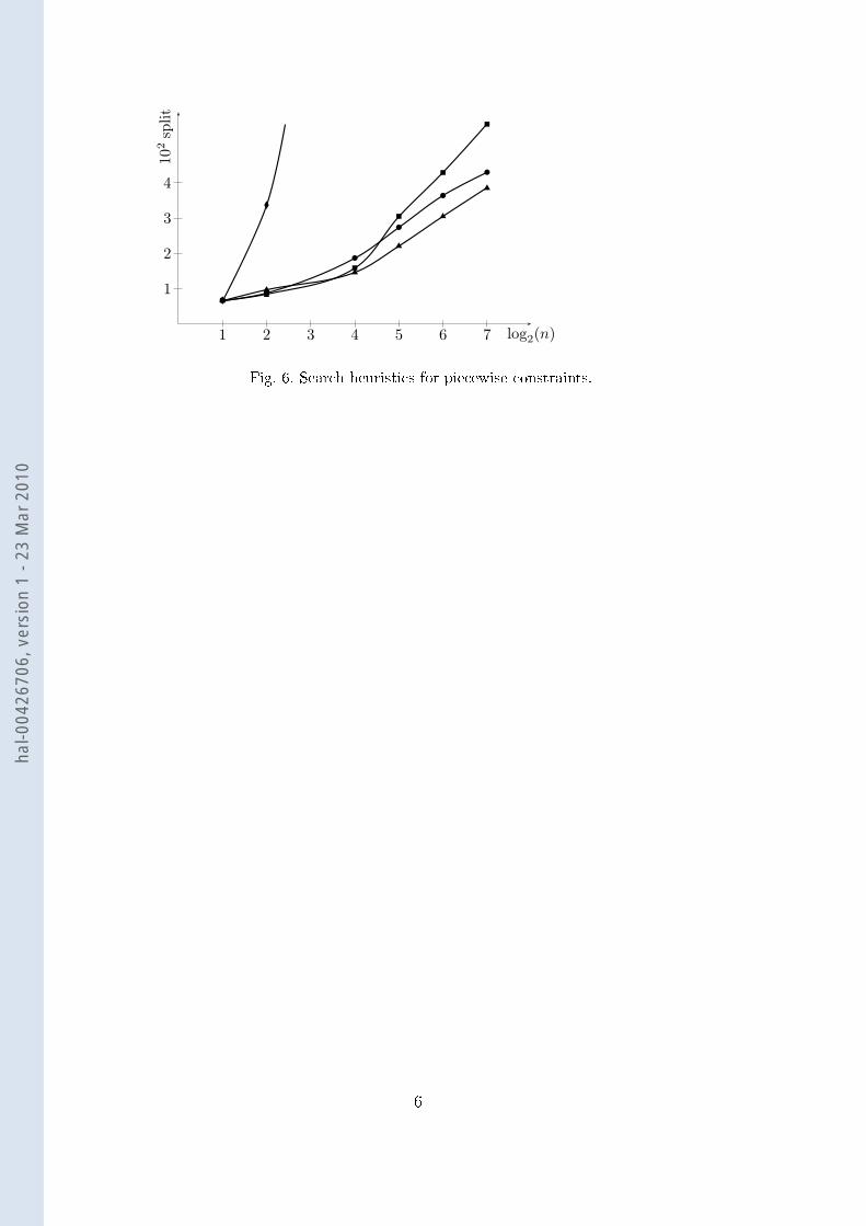
ternatively splits main and auxiliary variables with ratio r. We observe anexponential behavior when r in reases, i.e., when auxiliary variables are sel-dom split. We also noti e for this problem that labeling is better than bise tionon n. In fa t n must be set before solving the whole problem.The number of splitting steps on auxiliary variables should follow the hardnessof the problem on these variables. This theoreti al riterion is implementedhere by a global ratio on the variable sets. This ratio aims at favoring mainvariables a ording to the existential quanti�er whi h is de�ned on auxiliaryvariables, when onsidering an ED problem.4.3 Pie ewise onstraintsWe onsider the following problem:

(x, y, z) ∈ [−10, 10]3

y + y2 = z2 + 2

xz = z2 − 1

piecewise(x, I1 : mid(I1) = x2 − y2 + x,... ...In : mid(In) = x2 − y2 + x )

(11)25

hal-0

0426

706,

ver

sion

1 -

23 M

ar 2

010

where n is the number of pie es of the pie ewise onstraint, ea h interval Ik isde�ned byIk =

[

−10 + 20k − 1

n+ ν,−10 + 20

k

n− ν

]

, 1 ≤ k ≤ n, (12)ν > 0 is equal to the ma hine pre ision, and mid(Ik) is the midpoint of Ik.Let 10−8 be the pre ision of every variable.Figure 6 depi ts the number of splitting steps required for solving the problemparametrized by the number of pie es of the pie ewise onstraint. The variablesare hosen following a round robin strategy. The � urve is su h that only the�rst pruning ase of the pie ewise onstraint is applied. A restri ted pruningalgorithm is learly not e� ient. In this ase, many approximate solutionsin lude pie e bounds and the pie ewise onstraint is useless. The • urve orresponds to a full pruning algorithm with lassi al bise tion, the � one toa full pruning algorithm with split on the �rst hole from the domain of x, andthe N one to a full pruning algorithm with split on the mid hole. Bise tion ismore e� ient than split on the �rst hole. It is known that bise tion is moree� ient than labeling for ontinuous variables. Split on the mid hole is thebest heuristi s. The orresponding fun tion follows np with 0 < p < 1. Thenew te hnique seems e�e tive even for huge pie ewise onstraints.5 Empiri al evaluation on real-world problemsIn this se tion we evaluate our approa h on models obtained for real worldappli ations in me hani al engineering. It may be noted that the next resultsdo not take into a ount the existen e proof algorithm, be ause of the huge26

hal-0

0426

706,

ver

sion

1 -

23 M

ar 2

010

number of omputation steps it adds. Moreover we are mainly interested instudying our sear h heuristi results.5.1 A basi bat h-ex hanger systemWe �rst onsider a bat h ex hanger model (see Figure 7). The solution prin i-ples are de�ned using �ve design variables (three atalogs related to lengths,materials and diameters, the number of �ns, and the gap between �ns). In thismodel, the variables relating to the hoi es within atalogs are design variablesinstead of the length and materials of �ns and the diameter of the tube, whi hones have their values dire tly de�ned by the atalog. This problem is inter-esting from an ED point of view, sin e we have to hoose several omponentsin a (small) atalogs, while dimensioning the gap between �ns. In this sys-tem, there is a oupling between �uid me hani s and the geometry of the heatex hanger (namely the gap between �ns). System modeling introdu es �veauxiliary variables and �ve fun tional variables. The bat h-ex hanger is partof a bat h- ooler system for aperitif and this model investigates the feasibilityto ool down the aperitif from 25◦C to 8◦C in less than 25 se onds.Figure 8 depi ts the number of splitting steps using the robust strategy withratio r. The number of solutions is half of the number of splitting steps. The � urve omes from labeling of integer domains and the N urve from bise tions.We see that a high splitting ratio allows to de rease the number of splittingsteps. Due to some orientation in the model the auxiliary variables are dire tly omputed from the design variable values. Splitting auxiliary variables leads todupli ate solutions and onsequently useless sear h steps. Bise tion on integervariables is better than labeling. That is explained by e� ient redu tions of27

hal-0

0426

706,

ver

sion

1 -

23 M

ar 2

010

the number of �ns (integer in [5, 20]) using some bound onsisten y method.5.2 A pump and tank water ir uitThis model takes into a ount three tanks (one upstream and two downstream)and one water pump (see Figure 9). The obje tive is to study the feasibility ofdimensioning the two lines diameters after the downstream Y-bran h. Beforethe Y-bran h, the lines diameter is 0.055 meter. All the lines lengths are �xedand the two downstream tanks must re eive the same �ow, onsidering thatthe sum of the global lines se tion is the same before and after the Y-bran h.The water pressures in the tanks are de�ned initially: the upstream tank isat 40000 pas al and the two downstream tanks are open to the atmosphereair and the pressure is 101325 pas al. The pump is standardized and has hara teristi s (e� ien y, manometri head and required net positive su tionhead for a water �ow, et .) given by its manufa turer. The net positive su tionhead is investigated to guarantee the safety of the pump. The solutions are omputed taking into a ount that the avitation phenomenon in the pumpmust not appear, otherwise it may be seriously damaged. The downstream ir uit (dire tly linked to the avitation phenomenon) is oupled to the whole ir uit (pressure losses) and the Y-bran h make the problem non trivial.This model is made of two design variables (the two tube diameters after theY-bran h), three auxiliary variables and thirty-�ve fun tional variables. The�gures 10, 11, 12, 13, 14 and 15 depi t the results obtained when fun tionalvariables are split onsidering a global varying pre ision. Sin e the three aux-iliary variables have a �xed pre ision, a global pre ision an be de�ned onthe other variables, i.e. fun tional variables and they are split like auxiliary28

hal-0

0426

706,

ver

sion

1 -

23 M

ar 2

010

variables. Half of those pi tures depi ts the numbers of splits and the otherthe numbers of solutions. The • urves show the results obtained with a las-si al round-robin strategy for the hoi es on all variables (main, auxiliary andfun tional variables). The � urves express the results with a strategy alwaysstarting with main variables. On e they rea h the required pre ision, auxiliaryare variables split. The N urves represent the results with a hoi e strategywith a ratio de�ning a priority of 3 for the main variables on the auxiliaryvariables. Only results found within a reasonable time are written out on ea h urve: results with a solving time ex eeding one hour are not taken into a - ount.The �gures 10 and 11 represent the most general ase and all the fun tionalvariables are de�ned with the same global pre ision. The di�erent number ofsolution between ea h run an be explained by the mis ellany of the dupli- ation of design solutions and the powerlessness of onsisten y algorithm onintervals, whi h never remove real solutions, but have di� ulty to prune a u-rately some domains and to reje t them if they are near a real solution. In this ontext, the most a urate pre ision on fun tional variables given reasonablesolving time is 10−1. The • urve seems to have the worst results, in parti ularfor the more a urate pre ision, but otherwise the results are fairly similar. Itmay be noted that merging all the omputed solutions gives only one designar hite ture. Considering that fa t, the best omputing run is obtained by theN urve with 3 solutions and 296 splits for a fun tional variables pre ision of103. The best approa h onsidering the whole urves seems to be the N urve,where a robust strategy is applied.After these �rst results, we an observe that the pre ision 103 and 104 for fun -tional variables give good results. These quantities are ompatible with some29

hal-0

0426

706,

ver

sion

1 -

23 M

ar 2

010

fun tional variables values: losses in lines expressed in pas al and Reynoldsnumber values. So the �gures 12 and 13 give results where these fun tionalvariables have several �xed pre isions. In this ase, the most a urate pre isionis 10−10. Globally the • urve seems to be again the worst approa h, althoughit gives the smallest number of solutions after a pre ision of 10−7 for the samequantity of splits than others. The lowest number of solutions is given by the� with 3 solutions for 148 splits for a pre ision of 100. Previously the samesmall number of solutions was found, but in 296 splits.From the maximum pre ision to 101 the results stay the same, but until 10−2the number of solutions and the number of splits de rease. We an on ludethat some other fun tional variables values are ompatible with these pre i-sions. Then set pre isions are also given for the net positive su tion head andthe total manometri head and all surfa es. The �gures 14 and 15 show theresults obtained with all these set pre isions and with only a few still using thevarying global pre ision. In this ase, the robust strategy fails to give all thesolutions within reasonable time after a pre ision of 10−8, although it seems togive the best results before a global pre ision of 10−3. The two other urves al-low a maximum pre ision of 10−11 and up to a pre ision of 10−7 the results areinteresting. The best run is obtained by the � urve with 3 solutions and 148splits for pre isions of 100 and 10−1, whi h is not better than in the previous ase.With these results, we an on lude that fun tional variables have to be split(using CSP based on interval arithmeti ). But it is di� ult to de�ne arefullythe pre ision on ea h fun tional variable. If the quantities represented by theirvalues are known by designers, well de�ned pre isions an be set, but otherwisefew splits are better not to dupli ate main variables solutions.30

hal-0

0426

706,

ver

sion

1 -

23 M

ar 2

010

5.3 A bootstrap problemA basi model of an air raft onditioning system is investigated (see Figure 16).Air oming from a turbo-rea tor and from the atmosphere is used to produ e old air. The atmosphere air ools down the air oming from the turbo-rea torthrough a heat ex hanger where omplex pie ewise de�ned physi s phenomenaare studied (Fanning fri tion fa tor and Nusselt number). Turbo-rea tor air�ow passes through a ompressor to improve the heat transfer phenomenoninside the ex hanger. Before exiting the air onditioning system, a turbinereleases its pressure and makes its temperature de rease. A oupling shaft onveys the turbine me hani al energy to the ompressor. This problem is dif-� ult to solve sin e many physi s phenomena interfere. The loop orrespondingto the bootstrap make its omponents oupled a ording to the temperaturesand pressures of the air �ux. These temperatures and pressures are also linkedto the heat ex hanger geometry (gap between plates).In this model, the ompressor, the turbine and the oupling shaft are stan-dardized omponents and only the heat ex hanger has to be embodied as itmainly determines the air- onditioning performan es. The main obje tive ofthe system is to bring air to the passengers and the rew of the air raft and to ontrol the air temperature and pressure inside the o kpit. But some other riteria are important in an air raft, as the air �ow taken from the turbo-rea tor (that de reases its e� ien y), the in rease of the air raft drag, theweight of the air- onditioning system, et . This problem is e� iently solvedwith pie ewise onstraints: 6734 splitting steps and 1262 approximate solu-tions with respe t to 36978 splitting steps and 18860 approximate solutionswithout pie ewise onstraints. 31

hal-0

0426

706,

ver

sion

1 -

23 M

ar 2

010

Moreover this problem annot be solved within reasonable time with lassi alround-robin strategies on all the variables. The sear h spa e is so wide, thatif the embodiment design knowledge about main variables is not used, thesolving pro ess be omes very long. The use of fun tional variables with in�nitepre ision is the easiest way, sin e the model is omplex and fun tional variablesvalues quantities an hange. For instan e, the Reynolds number takes itsvalues from 100 to 200000.It may be noted in the solution set of these real problems, that auxiliaryvariables pre ision are often large. Indeed the interval approa h may omputeinterval solutions, where ea h one may ontain several solutions over the realnumbers. If the model is very sensitive to main variables values and if theirpre isions are not small enough, auxiliary variables may have large domainssin e they orrespond to the several main variables real values, whi h are ontained in one interval. From the designers' point of view and in the ontextof ED, it does not matter, be ause the main goal is to investigate the feasibilityof design on epts. Designers' �rst interest is to know where there is no solutionin the sear h spa e. If they want to have more pre ise auxiliary variables valuesfor one spe i� design ar hite ture, they just have to hange all variablesdomains orresponding to one or several omputing solution values and thento in rease main variables pre ision. They an start a new solving step on thismore restri ted sear h spa e and �nd more a urate values.6 Related workConstraint te hniques may be used at two su essive stages of preliminary de-sign. Dis rete onstraints may lead to determine the ar hite ture of a produ t32

hal-0

0426

706,

ver

sion

1 -

23 M

ar 2

010

during the on eptual design phase (O'Sullivan, 2001). CD using omponentsfrom the shelf is known as on�guration. These problems an be represented bydynami onstraint satisfa tion problems (Mittal & Falkenhainer, 1990) su hthat the involved omponents are a tivated and the orresponding onstraintsare solved. The notion of omponent (or variable) a tivation an be ta kled by onditional onstraints (Gelle & Faltings, 2003; Sabin et al., 2003). Larger andmore omplex problems are also ta kled by (Stumptner et al., 1998; Mailharro, 1998). From a solving point of view the main goal is to e� iently traversethe tree of ar hite tures. Numeri al nonlinear onstraints are more involved inthe ED phase. The frontier between CD and ED may be thin be ause mixed onstraints an be onsidered (Gelle & Faltings, 2003) to ta kle both phasesat the same time. But the ED physi s models are in general more omplex.Sam-Haroud & Faltings (1996) have proposed to represent numeri al on-straints by 2k-trees, namely de ompositions of the feasible regions using in-terval boxes. Strong onsisten y te hniques have been de�ned through the ombination of 2k-trees. Design appli ations su h as bridge design have beene� iently solved. In this framework, onstraint systems are de omposed inbinary and ternary onstraints in order to limit the size of 2k-trees (quadtreesif k = 2 and o trees if k = 3).Classi al interval te hniques have been implemented in the ED platform Con-straint Explorer (Zimmer & Zablit, 2001). The solving engine ombines in-terval arithmeti , onstraint propagation and sear h. An important feature isthe analysis of the onstraint network using graph de omposition (Bliek et al.,1998). The result of this analysis is an ordering of variables to be �xed beforesolving the asso iated onstraint blo ks. Re ent developments an be foundin (Neveu et al., 2006). Our approa h an be dire tly integrated for solving33

hal-0

0426

706,

ver

sion

1 -

23 M

ar 2

010

one blo k. In parti ular large blo ks may arise in ED models, for instan e inthe study of the equilibrium of a system.Pie ewise onstraints an be implemented by means of onditional onstraints(Zimmer & Zablit, 2001). This method amounts to the �rst ase of our pruningalgorithm. More re ently, binary pie ewise onstraints with pie es in the formof (x, y) ∈ Ik × Jk : Ck(x, y) have been represented by quadtrees (Vareilles etal., 2005). It seems di� ult to extend this approa h to onstraints of higherarities, whi h is required for solving the problems des ribed in this paper.Solution sets with nonzero volumes may be hara terized by inner approxima-tions, namely interval boxes of whi h every point is a solution. Several workshave ta kled spe i� ases: inequality onstraints by means of 2k-trees (Sam-Haroud & Faltings, 1996), interval boxes (Collavizza et al., 1999) or the ex-treme vertex representation (Vu et al., 2005), and equality onstraint systemswith at least as many existential quanti�ers as equations (Goldsztejn & Jaulin,2006). The study of su h te hniques for more heterogeneous onstraint systemsis an issue.Other works have taken into a ount relations that are not des ribed by an-alyti al expressions (Yannou et al., 2003; Fis her et al., 2004), exploiting inthe onstraint framework simulation results or data from bla k box numeri altools. The main idea is to ompute approximate onstraint-based models ofthese relations. 34

hal-0

0426

706,

ver

sion

1 -

23 M

ar 2

010

7 Con lusionED problems have been represented by onstraint satisfa tion problems withexistential quanti�ers. ED knowledge on types of variables and pre isions hasbeen used to improve the solver e� ien y. New sear h heuristi s based on asplitting ratio have been introdu ed to ta kle the quanti�ed variables. Dupli- ated solutions of main variables disappear and de isions on the design solu-tion prin iples set are easier to make for designers. A global onstraint hasbeen de�ned for pie ewise de�ned physi s phenomena. Experimental resultsfrom a ademi and real-world problems are promising. Embodiment designgoals are better taken into a ount sin e the main purpose is to investigatethe feasibility of the sear h spa e.There are many dire tions for future resear h. The notion of splitting ratio ould be re�ned to ta kle the hardness of every variable. The hardness of a vari-able should be learly de�ned. For instan e, dependen ies between variablesmay also indi ate variables relevan y in the model and possibly parti ipate totheir hardness. Auxiliary variables pre ision and solutions validation ould bemore studied. The notion of pre ision is essential in numeri al omputations.The pre ision on auxiliary variables is not often hosen appropriately and itindu ed many useless omputations steps in all heuristi sear h. The pre isionon main variables is easily de�ned onsidering the design knowledge about themodel: epistemi knowledge about main variables values. On the other hand,auxiliary variables are often part of omplex mathemati al expression. In fa t,the sensitivity of ea h variable should be investigated and pre ision should bede�ned onsidering the numeri al analysis of ea h onstraint in whi h variablesare involved. Nevertheless in pra ti e, it is very di� ult to apply and designers35

hal-0

0426

706,

ver

sion

1 -

23 M

ar 2

010

have no time to investigate in those fastidious al ulations. Moreover, the in-tegration of our te hniques in a blo k solving approa h ould be explored. Theblo k de omposition of a CSP takes into a ount the onstraints network andestablished an order or a ausality on variables or blo ks of variables based onthis network. In most design models, starting variables are needed to omputea relevant order, sin e models are often under- onstrained. Several orders onvariables may be de�ned for the same onstraint graph, and the hoi e of theoptimal one is unde idable within reasonable time(Jégou & Terrioux, 2003),but the main variables heuristi may help in this ordering task, taking intoa ount design knowledge.Referen esBeame, P., Cook, S., Edmonds, J., Impagliazzo, R., and Pitassi, T. (1995). Therelative omplexity of NP sear h problems. In Pro eedings of the Twenty-Seventh Annual ACM Symposium on theory of Computing (Las Vegas,Nevada, United States, May 29 - June 01, 1995). STOC '95. ACM Press,New York, NY, 303-314.Blum, C., & Roli, A. (2003), Metaheuristi s in ombinatorial optimization :Overview and on eptual omparison. ACM Computing Surveys, 35(3):268-308.Benhamou, F., Goualard, F., & Granvilliers, L., & Puget, J.-F. (1999). Revis-ing Hull and Box Consisten y. In International Conferen e on Logi Pro-gramming, pages 230-244. The MIT Press.Bliek, C., & Neveu, B., & Trombettoni, G. (1998). Using Graph De ompositionfor Solving Continuous CSPs. In CP'98, Pisa, Italy.Collavizza, H., & Delobel, F., & Rueher, M. (1999). Extending Consistent36

hal-0

0426

706,

ver

sion

1 -

23 M

ar 2

010

Domains of Numeri CSPs. In IJCAI'99, Sto kholm, Sweden.Cook, S., A., & Mit hell, D., G. (1997). Finding Hard Instan es of the Satis�a-bility Problem: A Survey. DIMACS Series in Dis rete Math. and Theoreti alComputer S ien e,35, 1997, pp1-17.Fis her, X., & Sébastian, P., & Nadeau, J.-P., & Zimmer, L. (2004). Constraintbased Approa h Combined with Metamodeling Te hniques to Support Em-bodiment Design. In SCI'04, Orlando, USA.Gelle, E., & Faltings, B. (2003). Solving Mixed and Conditional ConstraintSatisfa tion Problems. Constraints, 8:107-141.Goldsztejn, A., & Jaulin, L. (2006). Inner and Outer Approximations of Ex-istentially Quanti�ed Equality Constraints. In CP'06, Nantes, Fran e.Granvilliers, L., & Benhamou, F. (2006). Algorithm 852: Realpaver: An inter-val solver using onstraint satisfa tion te hniques. ACM TOMS, 32(1):138-156.Hyvönen, E. (1989). Constraint Reasoning Based on Interval Arithmeti . InIJCAI'89, Detroit, USA.Jégou, P., Terrioux, C. (2003). Hybrid ba ktra king bounded by tree-de omposition of onstraint networks. Arti� ial Intelligen e, vol. 146, pp.43-75.Kearfott, R. B. (1996). Rigorous Global Sear h: Continuous Problems. Non- onvex Optimization and Its Appli ations. Kluwer A ademi Publishers.Lhomme, O. (1993). Consisten y Te hniques for Numeri CSPs. In IJCAI'93,Chambéry, Fran e.Mailharro, D. (1998). A lassi� ation and onstraint-based framework for on-�guration. AI EDAM. 12(4). 383-397.Mittal, S. & Falkenhainer, B. (1990). Dynami Constraint Satisfa tion Prob-lems. In AAAI'90, Boston, USA. 37

hal-0

0426

706,

ver

sion

1 -

23 M

ar 2

010

Moore, R. (1966). Interval Analysis. Prenti e-Hall.Neveu, B., & Chabert, G., & Trombettoni, G. (2006). When Interval AnalysisHelps Interblo k Ba ktra king. In CP'06, Nantes, Fran e.O'Sullivan, B. (2001). Constraint-Aided Con eptual Design. Professional En-gineering Publishing.Pahl, G., & Beitz, W. (1996). Engineering Design: A Systemati Approa h.Springer.Ri hardson, D. (1968). Some Unsolvable Problems Involving Elementary Fun -tions of a Real Variable. Journal of Symboli Logi , 33, 514�520.Rossi, F., & van Beek, P., & Walsh, T. (2006). Handbook of Constraint Pro-gramming. Elsevier.Rothwell, R., & Gardiner, P. (1990). Robustness and Produ t Design Fami-lies, Design Management: A Handbook of Issues and Methods, pp. 279-292.(Oakley, M., ed.), Basil Bla kwell In ., Cambridge, MASabin, M., & Freuder, E. C., & Walla e., R. J. (2003). Greater E� ien y ofConditional Constraint Satisfa tion. In CP'03, Kinsale, Ireland.Sam-Haroud, D., & Faltings, B. (1996). Consisten y Te hniques for Continu-ous Constraints. Constraints, 1:85-118.Sébastian, P., & Chenouard, R., & Nadeau, J.-P., & Fis her, X.(2006). TheEmbodiment Design Constraint Satisfa tion Problem of the BOOTSTRAPfa ing interval analysis and Geneti Algorithm based de ision support tools,Pro eedings of Virtual Con ept 2006, Mexi o.Stumptner, M., & Friedri h, G., & Haselbö k, A. (1998). Generative onstraint-based on�guration of large te hni al systems. AI EDAM 12(4),307-320.Van-Hentenry k, P., & M Allester, D., & Kapur, D. (1997). Solving Polyno-mial Systems Using Bran h and Prune Approa h, SIAM Journal on Nu-38

hal-0

0426

706,

ver

sion

1 -

23 M

ar 2

010

meri al Analysis, vol. 34(2), p. 797-827.Vareilles, E., & Aldanondo, M., & Gaborit, P., & Hadj-Hamou, K. (2005).Using Interval Analysis to Generate Quadtrees of Pie ewise Constraints. InIntCP'05, Bar elona, Spain.Vu, X., & Sam-Haroud, D., & Silaghi, M. (2002). Approximation Te h-niques for Nonlinear Problems with Continuum of Solutions. In SARA'02,Kananaskis, Canada.Wang, P. S. (1974). The Unde idability of the Existen e of Zeros of RealElementary Fun tions. J. ACM 21, 4 (O t. 1974), 586-589.Yannou, B., & Simpson, T. W., & Barton, R. R.(2003). Towards a Con eptualDesign Explorer using Metamodeling Approa hes and Constraint Program-ming. In ASME DETC'03, Chi ago, USA.Zimmer, L. & Zablit, P. (2001). Global Air raft Predesign based on ConstraintPropagation and Interval Analysis. In CEAS-MADO'01, Koln, Germany.

39

hal-0

0426

706,

ver

sion

1 -

23 M

ar 2

010

A Bat h-ex hanger modelConstants names and values:The bat h volume ( l): V := 6Fin thi kness (mm): eail := 0.5Initial temperature of the aperitif (◦C): Ti := 20Final temperature of the aperitif (◦C): Tf := 8Volume of aperitif to ool down ( l): dose := 4Design Variables names, domains and pre isions:Catalog for the �ns materials (-): mater ∈ {1, 2}Catalog for the �ns length (-): ail ∈ {1, 2}Catalog for the tube diameter (-): diam ∈ {1, 2}Number of �ns (-): N ∈ [5..20]: integerSpa e between �ns (mm): e ∈ [1..4]: p(e) = 10−1Auxiliary variables names and domains:Time to ool down the aperitif (s): t ∈ [11..15]: p(t) = 10−1Tube diameter (mm): d ∈ [0..50]: Integer�ns length (mm): L ∈ [0..50]: IntegerFin ondu tivity (W/m/K): λ ∈ [1..200]: IntegerSaturation temperature (◦C): Tsat ∈ [−15..2]: p(Tsat) = 10−1Fun tional Variables names and de�nition:Surfa e of a semi �n (m2): Aail =L2

−π4·d2

10000001

hal-0

0426

706,

ver

sion

1 -

23 M

ar 2

010

Ex hanger surfa e (m2): A =N ·(2·Aail+

π·e·d1000000

)·dose

VEx hange oe� ient int the bat h-ex hanger (-): h = 1200eE� ien y oe� ient for a �n (-): fi = L−d

2000·√

2000·hλ

eailFin e� ien y (-): η =e(2·fi)−1

e(2·fi)+1

fiConstraints:Balan e of heat energy Tf = Tsat + (Ti − Tsat) · e−h·A·t·η

39doseBat h volume V = e · Aail · N · 100Catalog of tube diameters diam = 1 → d = 16

diam = 2 → d = 18Catalog of �n materials mater = 1 → λ = 200

mater = 2 → λ = 20Catalog of �n length ail = 1 → L = 40

ail = 2 → L = 50B Pump and tank water ir uit modelConstants names and values:Pressure in the upstream tank (pa): Pamont := 40000Pressure in the downstream tanks (pa): Paval := 101325Height of the verti al downstream line Hr1 := 5before the Y-bran h (m):Height of the verti al downstream line Hr2 := 2after the Y-bran h (m):Height of the verti al upstream line (m): Ha := 2Height of water in the upstream tank (m): Hw := 0.5Water density (kg/m3): ρ := 1e32

hal-0

0426

706,

ver

sion

1 -

23 M

ar 2

010

Water vis osity (m2/s): µ := 1e − 3A eleration due to gravity (m/s2) g := 9.81Lines diameter before the Y-bran h(m): D := 0.055Losses oe� ient in entry of upstream line: ξ1 := 0.5Losses oe� ient exiting downstream lines: ξ3 := 1Losses oe� ient in the Y-bran h towards ξ4 := 0.5the �rst downstream tank:Losses oe� ient in the Y-bran h towards ξ5 := 0.1the se ond downstream tank:Water temperature (◦C): T := 13Design Variables names, domains and pre isions:Line diameter after the Y-bran h towards Dr1 ∈ [0.02, 0.1]: p(Dr1) = 10−3the �rst downstream tank (m):Line diameter after the Y-bran h towards Dr2 ∈ [0.03, 0.1]: p(Dr2) = 10−3the se ond downstream tank (m):Auxiliary variables names and domains:Flow in the lines before the Y-bran h: Q0 ∈ [17/3600, 96/3600]: p(Q0) = 10−5Flow in the lines after the Y-bran h Qr1 ∈ [0, 96/3600]: p(Qr1) = 10−5towards the �rst downstream tank:Flow in the lines after the Y-bran h Qr2 ∈ [0, 96/3600]: p(Qr2) = 10−5towards the se ond downstream tank:Fun tional Variables names and de�nition:Se tion of ylindri al upstream lines S = π·D2

43

hal-0

0426

706,

ver

sion

1 -

23 M

ar 2

010

(m2):Se tion of ylindri al downstream lines Sr1 =π·D2

r1

4towards the �rst tank (m2):Se tion of ylindri al downstream lines Sr2 =π·D2

r2

4towards the se ond tank (m2):Surfa e of the verti al upstream line Ae1 = π · D · Ha(m2):Surfa e of the horizontal upstream line Ae2 = π · D · La(m2):Surfa e of the verti al downstream line Ae3 = π · D · Hr1before the Y-bran h (m2):Surfa e of the horizontal line towards Ae4 = π · Dr1 · Lr1the �rst downstream tank (m2):Surfa e of the verti al downstream line Ae5 = π · Dr2 · Hr2towards the se ond tank (m2):Surfa e of the horizontal line towards Ae6 = π · Dr2 · L2the se ond downstream tank (m2):Flowing speed in the lines before the V0 = Q0

SY-bran h (m/s):Reynolds number for the water before the Re1 = ρ·V0·DmuY-bran h (-):Pie ewise de�nition of Fanning fri tion Re1 ∈ [0, 2100] → f1 = 16

Re1fa tor for �owing before the Y-bran h: Re1 ∈ [2100, 50000] → f1 =

0.10512 · Re1−0.244

Re1 ∈ [50000, 1000000] → f1 =

0.04234 · Re−0.1641Reynolds number for the water between the Re2 =

ρ·Qr1Sr1

·Dr1

muY-bran h and the �rst downstream tank(-):De�nition of Fanning fri tion fa tor for Re2 ∈ [0, 2100] → f2 = 16Re24

hal-0

0426

706,

ver

sion

1 -

23 M

ar 2

010

�owing between the Y-bran h and the tank 1: Re2 ∈ [2100, 50000] → f2 =

0.10512 · Re−0.2442

Re2 ∈ [50000, 1000000] → f2 =

0.04234 · Re−0.1642Reynolds number for the water between the Re3 =

ρ·Qr2Sr2

·Dr2

muY-bran h and the se ond downstream tank (-):De�nition of Fanning fri tion fa tor for Re3 ∈ [0, 2100] → f3 = 16Re3�owing between the Y-bran h and the tank 1: Re3 ∈ [2100, 50000] → f3 =

0.10512 · Re−0.2443

Re3 ∈ [50000, 1000000] → f3 =

0.04234 · Re−0.1643Losses oe� ient in the upstream elbow ξ2 = 0.15 + 0.0175 · 4 · f1 · 2 · 90(pa):Losses oe� ient in the downstream elbow ξ6 = 0.15 + 0.0175 · 4 · f3 · 2 · 90(pa):Total manometri head (m): H = −1.1763 · 10−5 · (Q0 · 3600)3

−2.2052 · 10−4 · (Q0 · 3600)2+

1.4384 · 10−2 · (Q0 · 3600) + 21.554Net positive su tion head required: NPSHr = 1.2144 · 10−5 · (Q0·3600)3 − 1.2301 · 10−3 · (Q0·3600)2 + 4.9136 · 10−2 · (Q0 · 3600)

+0.49957Net positive su tion head available: NPSHa = Pamont−Psat

ρ·g+ (Ha+

2 · D) − DP0+DP1+DP2+DP3Ro·gWater saturation vapour pressure (pa): Psat = e23.3265− 3802.7T+273.18

−( 472.68T+273.18

)2Total losses in the ir uit (pa): ∆P = ∆P0 + ∆P1 + ∆P2 + ∆P3

+∆P4 + ∆P5 + ∆P6 + ∆P7Losses in entry of the verti al upstream line ∆P0 =ξ1·ρ·V 2

0

2(pa):5

hal-0

0426

706,

ver

sion

1 -

23 M

ar 2

010

Losses in the verti al upstream line (pa): ∆P1 = f1·Ae1

S3 · ρ·Q02

2Losses in the upstream elbow (pa): ∆P2 =ξ2·ρ·V 2

0

2Losses in the horizontal upstream line (pa): ∆P3 = f1·Ae2

S3 · ρ·Q20

2Losses in the verti al downstream line before ∆P4 = f1·Ae3

S3r1

· ρ·Q20

2the Y-bran h (pa):Losses in the Y-bran h towards the �rst ∆P5 =ξ4·ρ(

Qr1S

)2

2downstream tank (pa):Losses in the horizontal line towards the ∆P6 = f2·Ae4

S3r1

· ρ·Q2r1

2�rst downstream tank (pa):Losses exiting the line in the �rst ∆P7 =ξ3·ρ·(

Qr1Sr1

)2

2downstream tank (pa):Losses in the Y-bran h towards the se ond ∆P8 =ξ5·ρ·(

Qr2Sr2

)2

2downstream tank (pa):Losses in the verti al downstream line after ∆P9 = f3·Ae5

S3r2

· ρ·Q2r2

2the Y-bran h (pa):Losses in the elbow towards the se ond ∆P10 =ξ6·ρ·(

Qr2Sr2

)2

2downstream tank (pa):Losses in the horizontal line towards the ∆P11 = f3·Ae6

S3r2

· ρ·Q2r2

2se ond downstream tank (pa):Losses exiting the line in the se ond ∆P12 =ξ3·ρ·(

Qr2Sr2

)2

2downstream tank (pa):

6

hal-0

0426

706,

ver

sion

1 -

23 M

ar 2

010

Constraints:Y-bran h water �ow equality Qr1 + Qr2 = Q0

Qr1 = Qr2Downstream tubes se tion equality Sr1 + Sr2 = STotal manometri head H = Paval−Pamont

ρ·g− (Hw + Ha) + Hr1+

∆Pρ·gDownstream energy balan e ∆P5 + ∆P6 + ∆P7 == ∆P8 + ∆P9+

∆P10 + ∆P11 + ∆P12 + Hr2 · ρ · gNo avitation phenomenon NPSHa < NPSHrC Bootstrap modelConstants names and values:Flying altitude (m): Z = 10500Calori� apa ity di�eren e (J/kg/K): r = 287Mass apa ity ratio (-): τ = 10Plate ondu tivity (W/m/K): kp = 20Plate thi kness (m): tp = 0.001Mass �ow (kg/s): q = 0.7Isentropi e� ien y of the turborea tor's di�user (-): ηTRd = 0.9Compresion ratio of the turborea tor (-): TCTR = 8Isentropi e� ien y of the turborea tor's ompressor (-): ηTRc = 0.8Isentropi e� ien y of the ompressor (-): ηc = 0.75Isentropi e� ien y of the oupling shaft (-): ηAT = 0.95Isentropi e� ien y of the turbine (-): ηt = 0.8Heat apa ity ratio (-): γ = 1.4Ma h number (-): M = 0.87

hal-0

0426

706,

ver

sion

1 -

23 M

ar 2

010

Design Variables names, domains and pre isions:Width of the ex hanger (m): Lx ∈ [0.1..1]: p(Lx) = 10−2Spa ing between plates in the ex hanger (m): rh ∈ [0.001..0.1]: p(rh) = 10−3Auxiliary variables names and domains:Temperature between the ompressor and the ex hanger (K): T2 ∈ [0..1000]Temperature between the ex hanger and the turbine (K): T3 ∈ [0..1000]Temperature after the turbine (K): T4 ∈ [230..500]Pressure between the ompressor and the ex hanger (pa): p2 ∈ [0..10000000]Pressure between the ex hanger and the turbine (pa): p3 ∈ [0..10000000]Pressure after the turbine (pa): p4 ∈ [0..10000000]Mass �ow in the bootstrap (kg/s): q ∈ [0..1]Fun tional Variables names and de�nition:Length of the ex hanger (m): Ly = LxHeight of the ex hanger (m): Lz = 0.25 · LxTemperature of the atmosphere (K): Ta = 288.2 − 0.00649 · ZPressure of the atmosphere (pa): pa = 101290 · ( Ta

288.08)5.256Temperature between the di�user and the T0 = Ta · (1 + M2

·(γ−1)2

) ompressor of the turborea tor (K):Pressure between the di�user and the p0 = pa · (ηTRd · (M2·(γ−1)2

+ 1)γ

γ−1 ompressor of the turborea tor (pa):Temperature between the turborea tor T1 = T0 · (1 + 1ηTRc

· ((p1

p0)

γ−1γ − 1))and the ompressor (K):Pressure between the turborea tor and p1 = TCTR · p0the ompressor (pa):Porosity (-): σ = rh

(rh+tp)8

hal-0

0426

706,

ver

sion

1 -

23 M

ar 2

010

Reynolds number (-): Re = 4·rh·GµPrandtl number (-): Pr = 0.825 − 0.00054 · T2 + 5·

10−7 · T 22Nusselt number (-) pie ewise de�nition : Re ∈ [0, 2100] → Nu = 1.86·

(Pr·Re·2·rh

Lx)0.33

Re ∈ [2100, 8000] → Nu = 0.116·(Re0.66 − 125) · Pr0.33

Re ∈ [8000, 10000] → Nu = 10000−Re10000−8000

·0.116 · (Re0.66 − 125) · Pr0.33+

Re−800010000−8000

· 0.023 · Re0.8 · Pr0.33

Re ∈ [10000, 1000000] → Nu = 0.023·Re0.8 · Pr0.33)Fanning fa tor (-) pie ewise de�nition: Re ∈ [0, 2100] → f = 16 · Re−1

Re ∈ [2100, 100000] → f = 0.10512·Re−0.243

Re ∈ [100000, 10000000] → f =

0.04234 · Re−0.164)Air vis osity (kg/m/s): µ = −1.075 · 10−5 − 2.225 · 10−9 · T2+

1.725 · 10−6 ·√

T2Air thermal ondu tivity (W/m.K): λ = ((−2.620052386818974 · 10−6)·(T3+T2

2)2 + (9.169307749941458 · 10−3)·

(T3+T2

2) + 1.075874105919108 · 10−1)·

(10−2)Air density between the turboreator and ρ1 = p1

r·T1the ompressor (kg/m3:Air density between the ompressor and ρ2 = p2

r·T2the ex hanger (kg/m3):Air density between the ex hanger and the ρ3 = p3

r·T3turbine (kg/m3):9

hal-0

0426

706,

ver

sion

1 -

23 M

ar 2

010

Number of transfer units (-): Nut = H·Aq·CpEx hanger e� ien y (-): ǫ = 1 − eτ ·Nut0.22

·(e−1τ ·Nut0.78

−1)Ex hanger inlet pressure loss Ke = ((−0.00496672650332) · σ2+

(0.00113607587171) · σ+

(−0.00001379297260)) · ln(Re)2+

((0.06612031387891) · σ2+

(0.03340063900613) · σ+

(−0.00178687092114)) · ln(Re)+

(0.96233612367662) · σ2+

(−2.55595501972796) · σ+

1.01310287017856) oe� ient (-):Ex hanger outlet pressure loss Kc = ((0.00505236835109) · σ2+

(−0.00414707431984) · σ+

(0.00347507173062)) · ln(Re)2+

((−0.08548307647633) · σ2+

(0.06740608329495) · σ+

(−0.09241949837272)) · ln(Re)+

(−0.18282301765817) · σ2+

(−0.17962391485785) · σ+

1.00333194877608) oe� ient (-):Mass velo ity (kg/m2/s): G = qAfEx hange surfa e (m2): A = Lx·Ly·(Lz−2·rh−tp)

rh+tp2Flowing se tion (m2): Af = Ly · LzConve tive transfer oe� ient (W/m2/K): h = Nu·λ

rhGlobal heat transfer oe� ient (W/m2/K): H = 1

1/h+2·tpkpPressure loss in the ex hanger (pa): ∆pe = ( G2

2·ρ2) · (Kc + 1 − σ2) + f ·

( AAf

) · (2 · ρ2

ρ2+ρ3) + (Ke + σ2 − 1) · (ρ2

ρ3)10

hal-0

0426

706,

ver

sion

1 -

23 M

ar 2

010

Ex hanger volume (m3): V = Lx · Ly · LzPlate volume: Vp = A2· tpAir �owing speed in the ex hanger (m/s): C = q

Af ·ρ2Iron plate mass (kg): me = Vp · 7800Constraints:Compressor energy onservation: ηc · (T2

T1− 1) = (p2

p1)

γ

γ−1 − 1Coupling shaft energy onservation: (T2 − T1) = ηAT · (T3 − T4)Turbine energy onservation: 1 − T3

T4= ηt · (1 − (p3

p4)

γ−1γ )Ex hanger pressure loss: ∆pe = p2 − p3E hanger e� ien y ǫ = T2−T3

T2−T0

11

hal-0

0426

706,

ver

sion

1 -

23 M

ar 2

010

1 Figures

Fig. 1. Variables kind in the Embodiment Design phase.

1

hal-0

0426

706,

ver

sion

1 -

23 M

ar 2

010

102

103

104

105

106

0

0.02

0.04

0.06

0.08

0.1

0.12

0.14

0.16

Reynolds number values

Fan

ning

fric

tion

fact

or

f = 16/Re

f = 0.10512⋅Re−0.244

f = 0.04234⋅Re−0.164

Fig. 2. Fri tion fa tor as a fun tion of Reynolds number.

2

hal-0

0426

706,

ver

sion

1 -

23 M

ar 2

010

b

b

b

b

b

b

r r

r

r r

r

uu

u u

u u

n

log(s

plit)

3 4 5 6 7 8

2

3

4

Fig. 3. Sear h heuristi s for fun tional variables.

3

hal-0

0426

706,

ver

sion

1 -

23 M

ar 2

010

bb

b

b

b

b

rr

r

r

r

r

u uu

u

u

u

l l ll

l

l

n

103

splits

6 7 8 9 10 11

1

2

3

4

5

Fig. 4. Sear h heuristi s for fun tional variables.

4

hal-0

0426

706,

ver

sion

1 -

23 M

ar 2

010

u

u u u u u u u uu u u u

u

u

u

u

u

r

103

split

1 5 10 15

1

2

3

4

Fig. 5. Sear h heuristi s for auxiliary variables.

5

hal-0

0426

706,

ver

sion

1 -

23 M

ar 2

010

l

l

b

b

b

b

b

b

rr

r

r

r

r

u

u

u

u

u

u

1 2 3 4 5 6 7 log2(n)

102

split

1

2

3

4

Fig. 6. Sear h heuristi s for pie ewise onstraints.

6

hal-0

0426

706,

ver

sion

1 -

23 M

ar 2

010

Fig. 7. Bat h-ex hanger.r

r

r

rr r r r r r r r r r r

u

uu u u u u u u u u u u u u

r

103

split

1 5 10 15

1

2

3

Fig. 8. Solving the bat h-ex hanger problem.

7

hal-0

0426

706,

ver

sion

1 -

23 M

ar 2

010

Hw=0.5

Ha=2

La=1

Hr1=5

Hr2=2

L2=1

L1=1

R0/D=2

R0/Dr2=2

40000 pa

101425 pa

101425 pa

xi=0.1

xi=0.5

Y-branch

Fig. 9. Pump and tanks water ir uit.

8

hal-0

0426

706,

ver

sion

1 -

23 M

ar 2

010

b bb

b

b b

b

b

b

r r r

r

r

rr r

r

u u u

u

u

u

u u

u

Precision

log(s

plit)

+∞ 106 104 102 1 10−2 10−4 10−6 10−8 10−10

2

3

4

Fig. 10. Solving the pump problem with varying pre ision on fun tional variables.

b b b

b

b b

b b

b

r r r

r r

r r

r

r

u u uu

u

u uu

u

Precision

Nb

solu

tions

+∞ 106 104 102 1 10−2 10−4 10−6 10−8 10−10

50

100

150

Fig. 11. Solving the pump problem with varying pre ision on fun tional variables.

9

hal-0

0426

706,

ver

sion

1 -

23 M

ar 2

010

b bb

b bb b

b

b

bb

b

b

r r r r rr

rr

r

r

r

r

r

u u u

u u

uu

u

u

u

u u

u

Precision

log(s

plit)

+∞ 106 104 102 1 10−2 10−4 10−6 10−8 10−10

2

3

4

2

3

Fig. 12. Solving the pump problem with several �xed and varying pre isions onfun tional variables.

b b b b bb b

b

b

b

b

b

b

r r r r rr

r r

r

r

r

r

r

u u u u u

u u

u u

u

u

u

u

Precision

Nb

solu

tions

+∞ 106 104 102 1 10−2 10−4 10−6 10−8 10−10

100

250

500

750

Fig. 13. Solving the pump problem with several �xed and varying pre isions onfun tional variables.

10

hal-0

0426

706,

ver

sion

1 -

23 M

ar 2

010

b b bb

bb

bb b b

b

b

b

b

r r r rr

r rr r

r

r r

r

r

u u u u u u

u

u

u

u

u

Precision

log(s

plit)

+∞ 106 104 102 1 10−2 10−4 10−6 10−8 10−10

2

3

4

Fig. 14. Solving the pump problem with more �xed and fewer varying pre isions onfun tional variables than those shown in �gure 12 and 13.

b b b b b b b bb b

b

b

b

b

r r r r r r r r

r

r

r

r

r

r

u u u u u u

u

u

Precision

Nb

solu

tions

+∞ 106 104 102 1 10−2 10−4 10−6 10−8 10−10

100

250

500

Fig. 15. Solving the pump problem with more �xed and fewer varying pre isions onfun tional variables than those shown in �gure 12 and 13.

11

hal-0

0426

706,

ver

sion

1 -

23 M

ar 2

010

Fig. 16. Bootstrap �ux �ow diagram in an air raft.

12

hal-0

0426

706,

ver

sion

1 -

23 M

ar 2

010