Calculation of single fiber efficiencies for interception and impaction with superposed brownian...
19
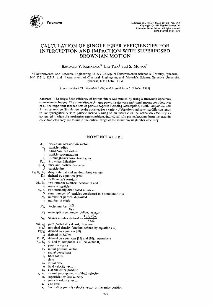
Pergamon J. Aerosol Sci., Vol. 25, No. 2, pp. 295 313, 1994 Copyright © 1994 Elsevier Science Ltd Printed in Great Britain. All rights reserved 0021-8502/94 $6.00 + 0.00 CALCULATION OF SINGLE FIBER EFFICIENCIES FOR INTERCEPTION AND IMPACTION WITH SUPERPOSED BROWNIAN MOTION BANDARU V. RAMARAO, *t CHI TIEN t and S. MOHAN* * Environmental and Resource Engineering, SUNY College of Environmental Science & Forestry, Syracuse, NY 13210, U.S.A. and , Department of Chemical Engineering and Materials Science, Syracuse University, Syracuse, NY 13244, U.S.A. (First received 21 December 1992; and in final form 5 October 1993) Abstract--The single fiber efficiency of fibrous filters was studied by using a Brownian dynamics simulation technique. This simulation technique permits a rigorous and simultaneous consideration of all the important mechanisms of particle capture including interception, inertial impaction and Brownian motion. Simulation results obtained for a variety of situations indicate that diffusion tends to act synergistically with particle inertia leading to an increase in the collection efficiency as compared to when the mechanisms are considered individually. In particular, significant increases in collection efficiency are found in the critical range of the minimum single fiber efficiency. A(t) ap b ¢ Cs DaM dr, dp F Fd, F~, F~ KU k Mi, Ni m mi, /1i N Nc /1 Npe NR Nst ~(0, y~) P(Yi) P(Yo) q R~, R~ R~, Ry r Co r rf t to u Uo ldx, /~y ¥ $o *o NOMENCLATURE Brownian acceleration vector particle radius Kuwabara cell radius particle concentration Cunningham's correction factor Brownian diffusivity fiber and particle diameters particle flux drag, external and random force vectors defined by equation (19d) Boltzmann's constant two random numbers between 0 and 1 mass of particles two normally distributed numbers total number of particles considered in a simulation run number of particle deposited number of trials usdf Peclet number -- DBM interception parameter defined as ap/rf Stokes number defined as Cs pp d 2 us 18/adr joint probability density function marginal density function defined by equation (37) defined by equation (38) defined as flkT/m defined by equations (12) and (10), respectively x- and y- components of the vector Rr position vector initial position vector radial coordinate fiber radius time initial time fluid velocity vector u at the entry position x- and y-components of fluid velocity superficial or face velocity particle velocity vector v at t=0 fluctuating particle velocity vector at the entry position 295
Transcript of Calculation of single fiber efficiencies for interception and impaction with superposed brownian...
Pergamon J. Aerosol Sci., Vol. 25, No. 2, pp. 295 313, 1994 Copyright © 1994 Elsevier Science Ltd
Printed in Great Britain. All rights reserved 0021-8502/94 $6.00 + 0.00
CALCULATION OF SINGLE FIBER EFFICIENCIES FOR INTERCEPTION AND IMPACTION WITH SUPERPOSED
BROWNIAN MOTION
BANDARU V. RAMARAO, *t CHI TIEN t a n d S. MOHAN*
* Environmental and Resource Engineering, SUNY College of Environmental Science & Forestry, Syracuse, NY 13210, U.S.A. and , Department of Chemical Engineering and Materials Science, Syracuse University,
Syracuse, NY 13244, U.S.A.
(First received 21 December 1992; and in final form 5 October 1993)
Abstract--The single fiber efficiency of fibrous filters was studied by using a Brownian dynamics simulation technique. This simulation technique permits a rigorous and simultaneous consideration of all the important mechanisms of particle capture including interception, inertial impaction and Brownian motion. Simulation results obtained for a variety of situations indicate that diffusion tends to act synergistically with particle inertia leading to an increase in the collection efficiency as compared to when the mechanisms are considered individually. In particular, significant increases in collection efficiency are found in the critical range of the minimum single fiber efficiency.
A(t) ap b ¢
Cs DaM
dr, dp F
Fd, F~, F~ KU
k Mi, Ni
m
mi, /1i N
Nc /1
Npe
NR
Nst
~(0, y~) P(Yi)
P(Yo) q
R~, R~ R~, Ry
r
Co r
rf t
to u
Uo
ldx, /~y
¥
$o
*o
N O M E N C L A T U R E
Brownian acceleration vector particle radius Kuwabara cell radius particle concentration Cunningham's correction factor Brownian diffusivity fiber and particle diameters particle flux drag, external and random force vectors defined by equation (19d) Boltzmann's constant two random numbers between 0 and 1 mass of particles two normally distributed numbers total number of particles considered in a simulation run number of particle deposited number of trials
usdf Peclet number - -
DBM
interception parameter defined as ap/rf
Stokes number defined as Cs pp d 2 us 18/adr
joint probability density function marginal density function defined by equation (37) defined by equation (38) defined as flkT/m defined by equations (12) and (10), respectively x- and y- components of the vector Rr position vector initial position vector radial coordinate fiber radius time initial time fluid velocity vector u at the entry position x- and y-components of fluid velocity superficial or face velocity particle velocity vector v at t = 0 fluctuating particle velocity vector at the entry position
295
296 B . V . RAMARAO et al.
U x ~ Uy X, y
XO, Yo Y¢
Ytlm Yi
G r e e k le t ters ot
At 6 g
( @
riD, rli, rh.i
rli.u ~i,I,D
0
pp O'vi, O'rl, 0"vr i
¢
x- and y-component of particle velocity Cartesian coordinate x- and y-coordinates of the entering particle position critical value of off-center distance off-center distance of the limiting trajectory at the entry point an arbitrary off-center distance value
packing density friction coefficient time interval delta function porosity unit fiber efficiency mean collection efficiency as calculated from the average of a number of simulation trials single fiber efficiency single fiber efficiencies due to Brownian diffusion, interception and combined interception and inertial impaction single fiber efficiency due to interception and diffusion from equation (36) single fiber efficiency due to interception, inertial impaction and diffusion according to equation (43) angular coordinate fluid viscosity particle density quantities defined by equations (14a)-(14c), respectively stream function
I N T R O D U C T I O N
The objective of this work is the development of a rigorous procedure which may be used for estimating the collection efficiencies of fibrous filtration under the combined effect of Brownian diffusion, inertial impaction and interception. The effectiveness of a filter medium in capturing aerosol particles is characterized by its single (or unit) fiber efficiency which is known to be dependent upon the collection mechanisms present in a given situation.
For the simple case where particle collection is dominated by a single mechanism such as interception or Brownian diffusion, it is often possible to obtain analytical expressions for the efficiencies. A more general approach of estimating collection efficiencies is the applica- tion of the so-called trajectory analysis which is used if the inertial impaction effect is not negligible. The trajectory analysis, however, can be applied only if all the forces acting on aerosols are deterministic. In other words, the trajectory analysis cannot be applied to determine collection efficiencies if the Brownian diffusion effect is significant.
The problem concerning the estimation of collector efficiency when more than one collector mechanism is important has occupied the attention of investigators in the past [see both Davis (1973) and more recently Pich (1987)]. The simplest (but not necessarily most accurate) approach is to assume that collection efficiencies due to individual collection mechanisms are additive or
N
~= ~ (~),, (1) i = !
where r/is the single fiber efficiency under the combined effect of N mechanisms and (r/)i is value of r/if only the ith mechanism is operative.
An alternate (and perhaps better) approach is to assume that penetration (defined as the effluent to influent concentration ratio) corresponding to a given situation may be ap- proximated by the product of penetrations due to individual mechanisms. For instance, this was applied by Kasper e t al . (1978) to study the penetration of a multistage diffusion battery. Under the condition that the filter medium is homogeneous, this approximation gives the following result
N
1--~/= I-I [1--(t/),]. (2) i = l
Single fiber efficiencies of fibrous filters 297
It is simple to show that equation (2) reduces to equation (10) if (~/)i<< 1 for all i. As pointed out by Pich (1987), there is no theoretical justification for either expression.
In the present work, we use a general method, based on the Brownian dynamics principle, which may be applied for estimating single fiber efficiencies when both deter- ministic and stochastic effects are present. In contrast to other available methods which may be used to solve problems of this type, this method has the advantage of being concep- tually simple and requires no use of extraneous assumptions. The development of this method also makes it possible to examine more closely the synergistic effect among the collection mechanisms and to assess the accuracies of the various approximate expressions including those of equations (1) and (2).
PREVIOUS WORK
The Brownian diffusion effect becomes pronounced for aerosols of diameter less than 1/~m. For this reason, submicron aerosols are often called diffusive aerosols. This termin- ology will be used through the present paper.
The simplest method of determining the single fiber efficiencies of diffusive aerosols in fibrous media is to view deposition as a mass transfer problem and to regard aerosols as a dissolving species in the gas phase (Friedlander, 1977). This method is limited to cases where particle collection is determined solely by Brownian diffusion. For the more general case where collection mechanisms other than Brownian diffusion may also be present, approximate relationships I-such as those of equations (1) and (2) as well as others; see Pich (1987) for more detailed information] have been used although their usage invariably introduced uncertainties and inaccuracies of unknown magnitude.
In more recent years, a number of methods aimed at a general analysis of the deposition of diffusive aerosols have been suggested. A review of this subject is available elsewhere (Ramarao and Tien, 1991a). Three of the more important methods which are relevant to the present study are listed below.
(1) Yuu and Jotaki (1978) proposed an approximate method for examining the combined effect of inertial impaction and Brownian diffusion on particle deposition in an ideal stagnation point flow. In their analysis, Yuu and Jotaki used the conventional convective diffusion equation as suggested by Friedlander but replaced the fluid velocity with the particle velocity which, in turn, was estimated from particle trajectory determinations assuming that the Brownian motion effect was negligible. The solution of the resulting hybrid convective diffusion equation gives the concentration fields and was used to provide estimates of the collection efficiency or deposition flux.
(2) Fernandez de la Mora and Rosner (1981, 1982) employed what may be termed as the continuum approach in their studies of particle deposition on a planar surface in a stagna- tion flow and on spherical and cylindrical collectors in Stokes' flow. The continuum approach considers a suspension to be composed of two continua: a fluid phase for which the equations of continuum mechanics hold and a particle phase which is characterized by a second set of flow equations.
(3) In contrast to the two methods mentioned above, a more direct way of treating the diffusive aerosol deposition problem is to solve the Langevin equations numerically. Such an attempt (often referred to as simulation based on Brownian dynamics) was used by Kanaoka et al. (1983) and Gupta and Peters (1985, 1986). Gupta and Peters' work was concerned with isolated spherical collectors while that of Kanaoka dealt with cylindrical collectors with Brownian diffusion as the only deposition mechanism (namely, without the inertial effect). The method of Brownian dynamics was applied to study the dispersion of particles injected to a uniform background flow by O'Brien (1990).
The present study is concerned with an investigation of the inertial effect of the deposition of diffusive aerosols on single cylindrical collectors (i.e. fiber). The study is therefore a generalization of the earlier work of Kanaoka et al. (1983). Although the results presented
298 B.V. RAMARAO et al.
here are single fiber efficiencies under the combined effect of Brownian diffusion, intercep- tion and inertial impaction, the method can easily be extended to include the presence of various types of surface interaction forces and can be applied to the study of hydrosol deposition as well.
EQUATIONS DESCRIBING AEROSOL DEPOSITION
The Lagrangian view of the particle motion may be generalized to include the diffusive motion of aerosols and provide a necessary framework (at least, in principle) for examining the combined effect of Brownian motion and other deterministic forces on particle depo- sition. In the Lagrangian approach, the trajectory of a given particle is determined by considering the forces and torques acting on the particle. The torque balance may be ignored since rotation of small spherical particles is generally insignificant.
A force balance on a particle gives the Langevin equation as follows
dv m ~ = F d + F ~ + F ~ , (3)
where v denotes the particle velocity vector and m and t are the particle mass and time. The forces consi£1ered are the drag force, the external force and the random force. Fr is taken to represent the combined effect of a large number of fluid molecular collisions experienced by the particle, which causes the random Brownian motion. In case F~ is insignificant, equation (1) may be integrated to give the trajectory of the particle for a given set of initial conditions (velocity and position).
The random force, Fr, may be written as the product of the particle mass and a random Brownian acceleration A(t). By doing so, the random nature of Fr(t) is now ascribed to A(t). We assume that A(t) is independent of v(t). Furthermore A(t) fluctuates rapidly as compared to the variations in v. The random acceleration A(t) has a mean of zero and its auto- correlation is an impulse function. Thus,
(A(t)) =0 (4)
(A(t) A(t + z)) = K f ( t - ~). (5)
A(t) is represented as a Gaussian white noise process in stochastic terms. The drag force experienced by a small spherical particle may be written as
Fd = mfl(U-- V), (6)
where fl is the friction coefficient, u and v are the fluid and particle velocity vectors. With the use of the Stokes law, fl is given as
fl = 6~#ap, (7) Csm
where ap is the particle radius,/z the fluid viscosity and cs the Cunningham correction factor. From equation (6), equation (3) may be rewritten as
~ = fl(U-- V) + Fe-t-A(t). (8) m
The solution of equation (8) can be readily obtained for the following special case; the fluid velocity is constant and fl is constant [as given by equation (7)] (Chandrasekhar, 1943; Gupta and Peters, 1985, 1986). For a particle with velocity v0, initially (i.e. t =0), integration of equation (8) gives
v = voe-Pt + u(1 - e-#t) + Fe (1 - e-~r) + Rv(t), (9) m
Single fiber efficiencies of fibrous filters 299
where
R~ (t) = f l ea t~ -,) A (0 d~. (10)
Substituting dr/dt for v in equation (9), with the initial condition r = ro at t = 0, one has
, 1 Vo --e - a ) + u t - - - (1 r = r o + ~ - ( 1 [ 13 - e - a ' ) ]
[ ' 'l +F.m t - ~ ( 1 - e - a ) +Rr(t), (11)
where
Rr(t)= fl I f~ e~¢ A(Od(]e-P" dn. (12)
Rv and Rr are two random deviates which are bivariate Gaussian distributed (Chandra- sekhar, 1943). The components of Rv and Rr can be calculated as follows
Rvi = 0-vi 0 n i Rr, 0-vri/0-~i 0-2 ~ 2 /rr2~1/2 mi (13)
r i - - - - l l r i l V O i !
0-2, = ~ (1 - e -2at) (14a)
0.2 q ,~- = ~ tz/Jt - 3 + 4 e - a t - e- 2at) (14b) Yi
0-vr, =~(1 -- e-at) 2 (14c)
#kT q-- , (15)
m
where k is the Boltzmann constant, n~ and m~ are two normally distributed numbers. Let N~ and M~ be two random numbers between 0 and 1. n~ and m~ can be found from the following relationship
1 /'~' A i = ~ J _ e-~/2d( , (16)
where A~ = N~ or Mi and ai = ni or mi. Standard computer software (for example, IMSL, 1982) is available for generating such
random numbers and calculating random deviates. For the general case where the fluid velocity is not constant, equations (9) and (11) can be
used to obtain particle trajectories numerically. For a sufficiently small time interval, At, the fluid velocity experienced by a particle may be assumed to be constant. For a given initial position and velocity, equations (9) and (11) can be used to obtain the particle's velocity and position at the end of the time interval by replacing t = At. This process may be repeated to obtain the particle's trajectory incrementally.
S I M U L A T I O N M E T H O D
Kuwabara flow field and definitions of collection efficiencies The Kuwabara flow field used in the simulation is based on the assumption that a fibrous
medium may be represented by a basic unit (unit cell) consisting of a single fiber of radius rf surrounded by a fluid envelope of radius b with fluid entering and leaving the outer cell along the direction transverse to that of the axis of the cylinder (see Fig. 1). The fluid
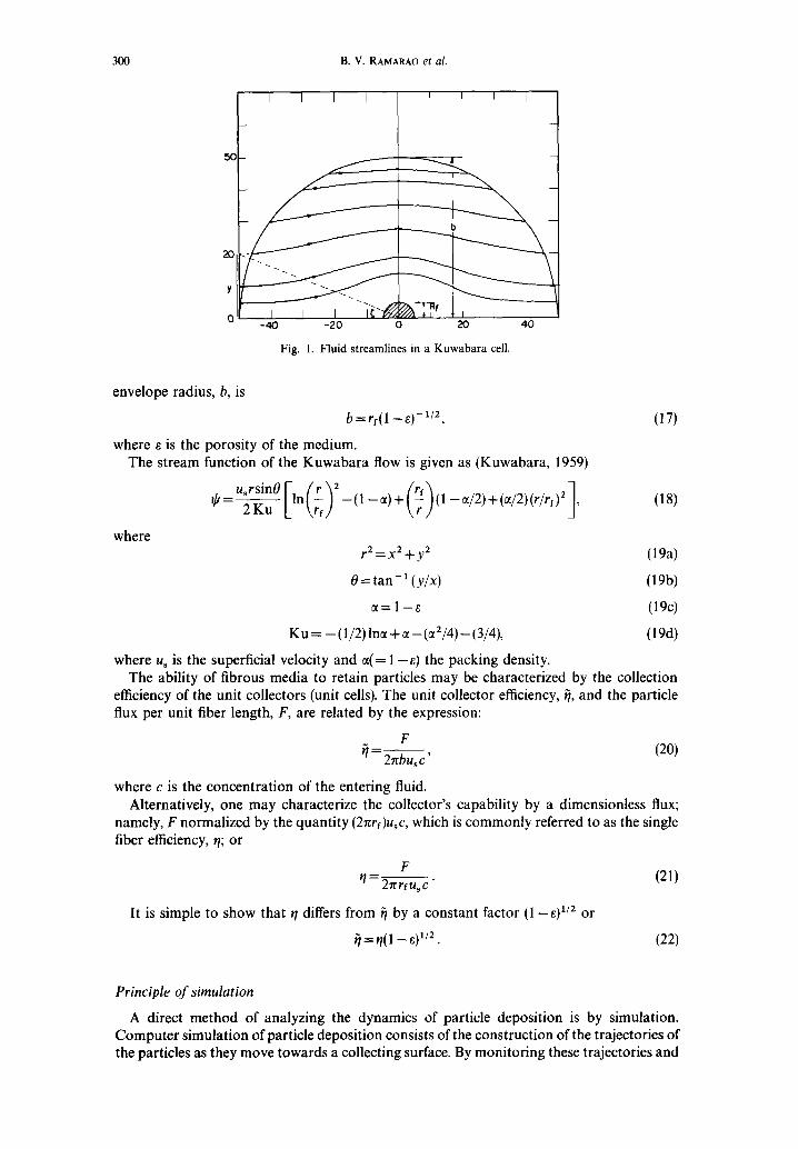
300 B.V. RAMARAO et al.
50
20
Y
O
r 7 - - ~ 1 - - - - F - -
-40 -20 0 20 40
Fig. 1. Fluid streamlines in a Kuwabara cell.
envelope radius, b, is
b = rf(1 - e ) - 1/2,
where e is the porosity of the medium. The stream function of the Kuwabara flow is given as (Kuwabara, 1959)
Ku L , r , /
where
(17)
(18)
r 2 = x 2 + y 2 (19a )
0 = tan- 1 (y/x) (19b)
~= 1 - e (19c)
Ku = - (1/2) ln~ + ~ - (~2/4)- (3/4), (19d)
where us is the superficial velocity and ~(= 1 - e ) the packing density. The ability of fibrous media to retain particles may be characterized by the collection
efficiency of the unit collectors (unit cells). The unit collector efficiency, ~, and the particle flux per unit fiber length, F, are related by the expression:
F rl = 2~bus c' (20)
where c is the concentration of the entering fluid. Alternatively, one may characterize the collector's capability by a dimensionless flux;
namely, F normalized by the quantity (21trf)usc, which is commonly referred to as the single fiber efficiency, ~/; or
F ~ l - - 2 r c r f u s c . (21)
It is simple to show that ~/differs from ~ by a constant factor (1 - -8) 1/2 o r
= t/(1 -- e) 1/2 . (22)
Principle of simulation
A direct method of analyzing the dynamics of particle deposition is by simulation. Computer simulation of particle deposition consists of the construction of the trajectories of the particles as they move towards a collecting surface. By monitoring these trajectories and
Single fiber efficiencies of fibrous filters 301
from the knowledge of whether or not they impinge upon the surface and hence become deposited and the positions of deposition if they do, both the macroscopic (namely, the unit or single fiber efficiency) and microscopic (local deposition flux and morphology of depo- sition) information of particle deposition may be obtained.
The steps involved in simulating particle deposition may be stated as follows (Tien, 1989): (a) identification of the spatial domain through which particles travel, (b) specification of the flow field around the collecting surfaces, (c) designation of the initial positions and velocities of the particles as they flow past the collector and (d) determination of particle trajectories.
In the present problem, the spatial domain is chosen to be a cylindrical envelope of fluid surrounding the typical fiber placed transverse to the flow direction. For a calculation of the initial or clean collector efficiency, it is sufficient to consider only one half of the cell on account of the symmetry of the flow that is to be expected. The flow field may be chosen to be the well known Kuwabara flow field [see e.g. Lee and Liu (1982)-1. The determination of the trajectories of the diffusive aerosols is made from the numerical integration of the Langevin equation based on the expression given by equations (9) and (11).
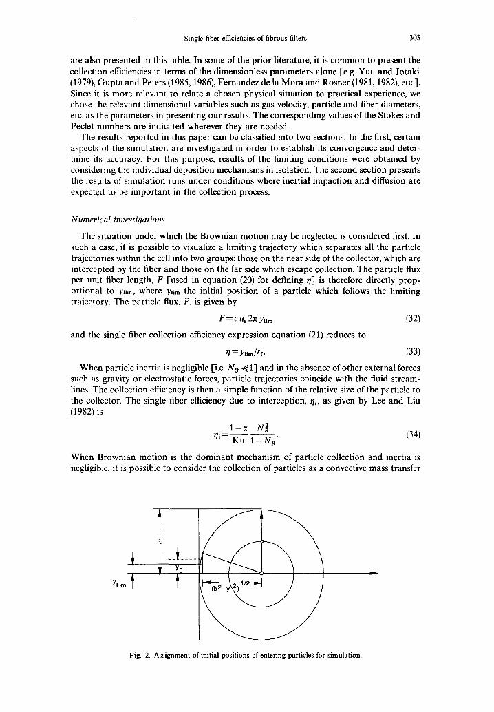
Specification of the initial conditions of entering particles
The initial position of a particle entering the Kuwabara cell is given by its off-center distance at the fluid envelope. In terms of a Cartesian coordinate with its origin located at the center of the collector, its coordinates are (see Fig. 2),
_ x=(b 2_y2)1/2 (23)
Y = Yo. (24)
Since the flow is two-dimensional, the entering aerosols may be assumed to be randomly distributed over the line segment at x = - b extending from y = 0 to y = b (as shown in Fig. 2). One can therefore designate the initial positions of the N entering particles by generating a sequence of uniformly distributed random numbers 0 < ni < 1, i = 1, 2 . . . . N by defining Yo to be
Yo = nib. (25)
The Brownian particles are assumed to be initially in thermal equilibrium with the gas. Thus, their initial velocities will be equal to that of the fluid at the initial location plus a fluctuating component due to the thermal motion. The particles' velocities can then be assumed to be given by a Maxwellian distribution as [see Gupta and Peters (1985, 1986) and Chandrasekhar (1943)],
Vo = u0 + v~, (26)
where u0 is the fluid velocity at ro and v6 is a Gaussian random variable with
(v~) =0 (27a)
kT ( v ~ v ~ ) = a f l - - . (27b)
m
Determination of particle trajectories
It is possible to integrate the Langevin equation under either of the following conditions: that the flow field, u(r), is (a) linear [Ramarao and Tien (1991a, b)] and, (b) constant. To apply the results of case (a), the actual flow field may be expanded in a Taylor's series and the solution is applied over a sufficiently small spatial domain over which the flow field is linear. On the other hand we may also assume a small enough time step such that the fluid velocity u(r) experienced by the particle over the time interval is constant as in conventional Brownian dynamics simulations [Gupta and Peters (1985, 1986), Ermak and McCammon
302 B.V. RAMARAO et al.
(1984), etc.]. Under this assumption, the solutions to the Langevin equat ion are
= vx, e - P A ' + - ~ ( 1 - -e -PA' )+Rvx (28a) /)x.i+ 1
= vr, e - SAt + ~ (1 -- e - p~t) + R ~ (28b) 1) y. i+ 1
xi+l=xi+~(1-e-pAt)+~[At-~(1-e-P~')]+R,x (29a)
y,+l=yi+~-[1-e-PAt]+~[At-~(1-e-Pa') l+R,, , (29b)
where Rw, Rvr, R,x and R,y are r andom variables as given in equat ion (13) and the subscript i denotes the values at t = iAt.
Once the initial condit ions of a particle are known, the trajectory can be constructed according to the above equations. This trajectory calculation terminates when the particle either exits from the fluid envelope or impacts on the fiber. At each time step, if the condit ion
2 2 x i + Y i ~< (rf + rp) 2 (30)
is fulfilled, the particle is assumed to impact the fiber.
Calculation of the unit collector efficiency For a given simulation, let N be the number of the approaching particles considered, of
which N~ particles are collected. The unit collector efficiency is
( N ¢ ) ( q ) = N ' (31)
where ( ) denotes the average value over a large number of trials. The corresponding single fiber efficiency, (q ) , can be readily found from the value of ( ~ ) and the relationship given by equat ion (22).
R E S U L T S
Simulation of particle collection was made for a number of representative situations. Table 1 gives the condit ions used for the simulation runs as well as the ranges of the relevant variables. The corresponding ranges of the dimensionless parameters (such as Ns, and Npe)
Table 1. Systems and operating variables used in simulation
Gas (air) properties Mean free path, 2 0.62 nm Pressure 1 ata Temperature, T 278 K Viscosity, # 1.83 × 10 -5 Pas Density, p 1.203 kg m- 3
Particles Density, pp 1000 kgm -3
Deposition conditions Face velocity, u~ 0.01-2 m s- 1 Packing density, ~ 0.014).1 Fiber diameter, df 10/~m
Dimensionless parameters Interception parameter, NR 10-3-0.1 Stokes number, Nst 10-4-1.0 Peclet number, Ne, 150-108
Single fiber efficiencies of fibrous filters 303
are also presented in this table. In some of the prior literature, it is common to present the collection efficiencies in terms of the dimensionless parameters alone [e.g. Yuu and Jotaki (1979), Gupta and Peters (1985, 1986), Fernandez de la Mora and Rosner (1981, 1982), etc.]. Since it is more relevant to relate a chosen physical situation to practical experience, we chose the relevant dimensional variables such as gas velocity, particle and fiber diameters, etc. as the parameters in presenting our results. The corresponding values of the Stokes and Peclet numbers are indicated wherever they are needed.
The results reported in this paper can be classified into two sections. In the first, certain aspects of the simulation are investigated in order to establish its convergence and deter- mine its accuracy. For this purpose, results of the limiting conditions were obtained by considering the individual deposition mechanisms in isolation. The second section presents the results of simulation runs under conditions where inertial impaction and diffusion are expected to be important in the collection process.
Numerical investigations
The situation under which the Brownian motion may be neglected is considered first. In such a case, it is possible to visualize a limiting trajectory which separates all the particle trajectories within the cell into two groups; those on the near side of the collector, which are intercepted by the fiber and those on the far side which escape collection. The particle flux per unit fiber length, F [used in equation (20) for defining ~/] is therefore directly prop- ortional to y~im, where y~im the initial position of a particle which follows the limiting trajectory. The particle flux, F, is given by
F = c us 2re Ylim (32)
and the single fiber collection efficiency expression equation (21) reduces to
17 = Y l i m / r f . (33)
When particle inertia is negligible [i.e. Nst,~ 1-] and in the absence of other external forces such as gravity or electrostatic forces, particle trajectories coincide with the fluid stream- lines. The collection efficiency is then a simple function of the relative size of the particle to the collector. The single fiber efficiency due to interception, rh, as given by Lee and Liu (1982) is
1--~ N 2 ~/i= Ku 1 +NR" (34)
When Brownian motion is the dominant mechanism of particle collection and inertia is negligible, it is possible to consider the collection of particles as a convective mass transfer
YLim
b
Fig. 2. Assignment of initial positions of entering particles for simulation.
304 B.V. RAMARAO et al.
process. Lee and Liu (1982) provided an expression for the collection efficiency due to Brownian motion by considering the convective diffusion mass transfer to the fibers in a Kuwabara flow field.
( 1 - - 0~'~ 1/3
qD=2"58\ Ku J N ~ z/3 . O5)
For the single fiber efficiency when diffusion and interception are acting simultaneously, r/i,o, if the approximation of equation (1) is used, r/i,o is given as (Lee and Liu, 1982)
r/i, o = qi + r/o. (36)
With negligible Brownian diffusion effect, particle trajectories in the inertial case are given by the solution of the Langevin equation [equation (8)] with the Brownian acceler- ation term omitted. In this case, the differential equation is deterministic and can be solved after substituting the Kuwabara flow field for u. We used a 6th order Runge-Kutta-Vernier method (IMSL subroutine DVERK) to solve the differential equation and obtain particle trajectories. Corresponding to a specified situation, the limiting trajectory was determined iteratively.
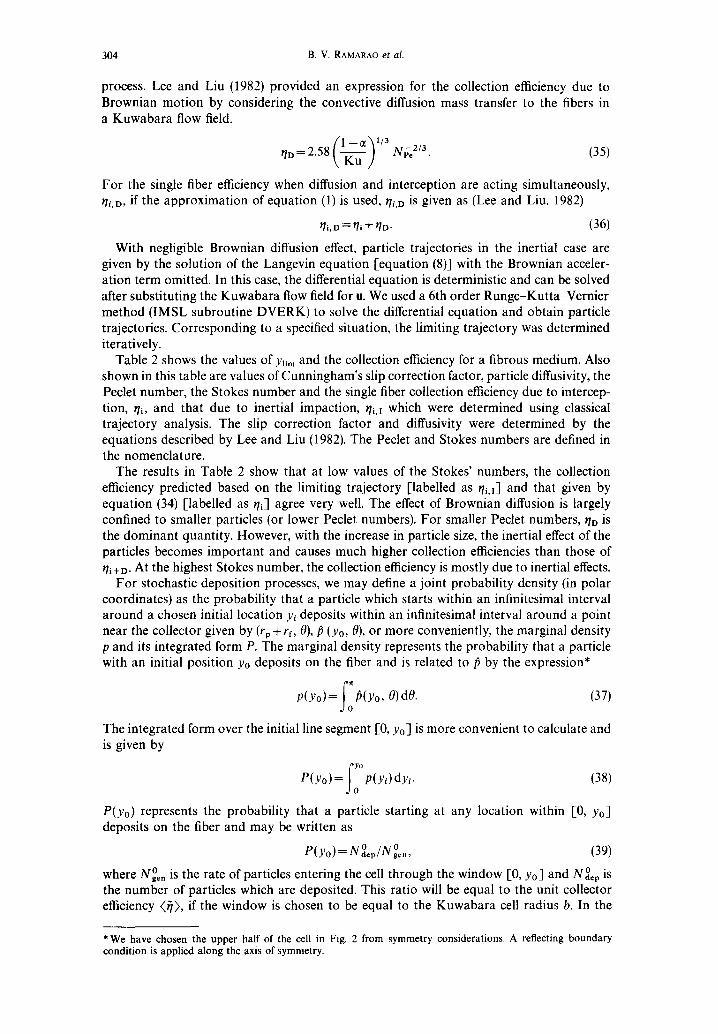
Table 2 shows the values of Ynm and the collection efficiency for a fibrous medium. Also shown in this table are values of Cunningham's slip correction factor, particle diffusivity, the Peclet number, the Stokes number and the single fiber collection efficiency due to intercep- tion, qi, and that due to inertial impaction, r/ia which were determined using classical trajectory analysis. The slip correction factor and diffusivity were determined by the equations described by Lee and Liu (1982). The Peclet and Stokes numbers are defined in the nomenclature.
The results in Table 2 show that at low values of the Stokes' numbers, the collection efficiency predicted based on the limiting trajectory [labelled as /']i,i] and that given by equation (34) [labelled as qi] agree very well. The effect of Brownian diffusion is largely confined to smaller particles (or lower Peclet numbers). For smaller Peclet numbers, r/D is the dominant quantity. However, with the increase in particle size, the inertial effect of the particles becomes important and causes much higher collection efficiencies than those of r/i + D. At the highest Stokes number, the collection efficiency is mostly due to inertial effects.
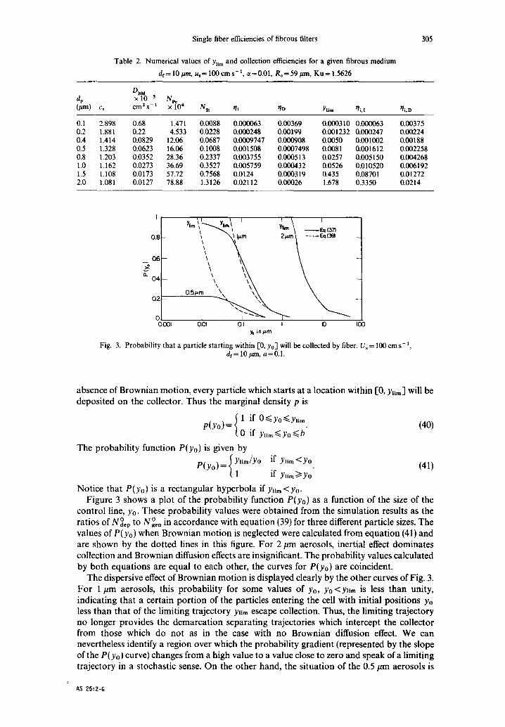
For stochastic deposition processes, we may define a joint probability density (in polar coordinates) as the probability that a particle which starts within an infinitesimal interval around a chosen initial location yl deposits within an infinitesimal interval around a point near the collector given by (rp + rf, 0),/~ (Yo, 0), or more conveniently, the marginal density p and its integrated form P. The marginal density represents the probability that a particle with an initial position yo deposits on the fiber and is related to/~ by the expression*
p(yo)=f£O(yo, 0)d0. (37)
The integrated form over the initial line segment [0, Yo] is more convenient to calculate and is given by
;? P(Yo) = p(y~) dye. (38)
P(Yo) represents the probability that a particle starting at any location within [0, Yo] deposits on the fiber and may be written as
o o P ( y o ) = N a e p / g g e , , (39)
where o Nge, is the rate of particles entering the cell through the window [0, Yo] and N°ep is the number of particles which are deposited. This ratio will be equal to the unit collector efficiency (~), if the window is chosen to be equal to the Kuwabara cell radius b. In the
* We have chosen the upper half of the cell in Fig. 2 from symmetry considerations. A reflecting boundary condition is applied along the axis of symmetry.
Single fiber efficiencies of fibrous filters
Table 2. Numerical values of YI~,, and collection efficiencies for a given fibrous medium
de = 10/~m, us = 100 cm s - 1, ~t = 0.01, R, = 59/tm, Ku = 1.5626
305
dp (/~m) c,
DBM x 10- s Np e
crn z s - 1 x 10⁴ Nst ~i ~D Ylim r/i,I ffi, D
0.1 0.2 0.4 0.5 0.8 1.0 1.5 2.0
2.898 0.68 1.471 0.0088 0.000063 0.00369 0.000310 0.000063 0.00375 1.881 0.22 4.533 0.0228 0.000248 0.00199 0.001232 0.000247 0.00224 1.414 0.0829 12.06 0.0687 0.0009747 0.000908 0.0050 0.001002 0.00188 1.328 0.0623 16.06 0.1008 0.001508 0.0007498 0.0081 0.001612 0.002258 1.203 0.0352 28.36 0.2337 0.003755 0.000513 0.0257 0.005150 0.004268 1.162 0.0273 36.69 0.3527 0.005759 0.000432 0.0526 0.010520 0.006192 1.108 0.0173 57.72 0.7568 0.0124 0.000319 0.435 0.08701 0.01272 1.081 0.0127 78.88 1.3126 0.02112 0.00026 1.678 0.3350 0.0214
I
Ytm ~ " ~ h m I Ylim \ c. (37) \ 2,.,,I . . . . O.8-
0.SPm ~ \ \ X k . _
o i O001 O01 OI I I0 100
y. inFm
Fig. 3. Probability that a particle starting within [0, Yo] will be collected by fiber. U, = 100 cm s - 1, d r= 10/zm, a=0.1 .
absence of Brownian motion, every particle which starts at a location within [0, Y~im] will be deposited on the collector. Thus the marginal density p is
p(y0)=~" 1 if 0~<yO~<Yli m (40) 0 if Ylim~Yo~b
The probability function P(Yo) is given by
p(yo)=~Ylim/Y o if Y.m<Y0. (41) ( 1 i f Ylim ~ YO
Notice that P(Yo) is a rectangular hyperbola if Y~i,. <Yo. Figure 3 shows a plot of the probability function P(Yo) as a function of the size of the
control line, Yo. These probability values were obtained from the simulation results as the ratios of N°ep to NO. in accordance with equation (39) for three different particle sizes. The values of P(Yo) when Brownian motion is neglected were calculated from equation (41) and are shown by the dotted lines in this figure. For 2/~m aerosols, inertial effect dominates collection and Brownian diffusion effects are insignificant. The probability values calculated by both equations are equal to each other, the curves for P(Yo) are coincident.
The dispersive effect of Brownian motion is displayed clearly by the other curves of Fig. 3. For 1/~m aerosols, this probability for some values of Yo, Y0 <Y,,, is less than unity, indicating that a certain portion of the particles entering the cell with initial positions Yo less than that of the limiting trajectory y,, , escape collection. Thus, the limiting trajectory no longer provides the demarcation separating trajectories which intercept the collector from those which do not as in the case with no Brownian diffusion effect. We can nevertheless identify a region over which the probability gradient (represented by the slope of the P(Yo) curve) changes from a high value to a value close to zero and speak of a limiting trajectory in a stochastic sense. On the other hand, the situation of the 0.5 #In aerosols is
AS 25:2-G
306 B.V. RAMARAO et al.
different. For low values of Yo, the probability of collection is nearly a constant but considerably lower than unity. A significant portion of the particles which originate at a location Yo less than Y,m escape collection. Similarly, a substantial fraction of the particles which originate at locations greater than yjlm may also deposit on the collector. The limiting trajectory, in this case, no longer has its conventional physical significance.
Intuitively, from the figure, we may conclude that the probability of deposition for a particle which originates at points far from the central axis diminishes with the distance. This fact can be used advantageously in reducing the amount of computations in simulation by choosing only a small window at the outer edge of the cell instead of the entire cell length. In other words, particles are introduced over an interval [0, Yo], where Yo is chosen such that the marginal probability of collection, P(Yo) is vanishingly small. For example, from Fig. 3, Yo may be chosen to be 1 #m in the 0.5 #m particles' case and 10 #m in the 2 #m particles' case.
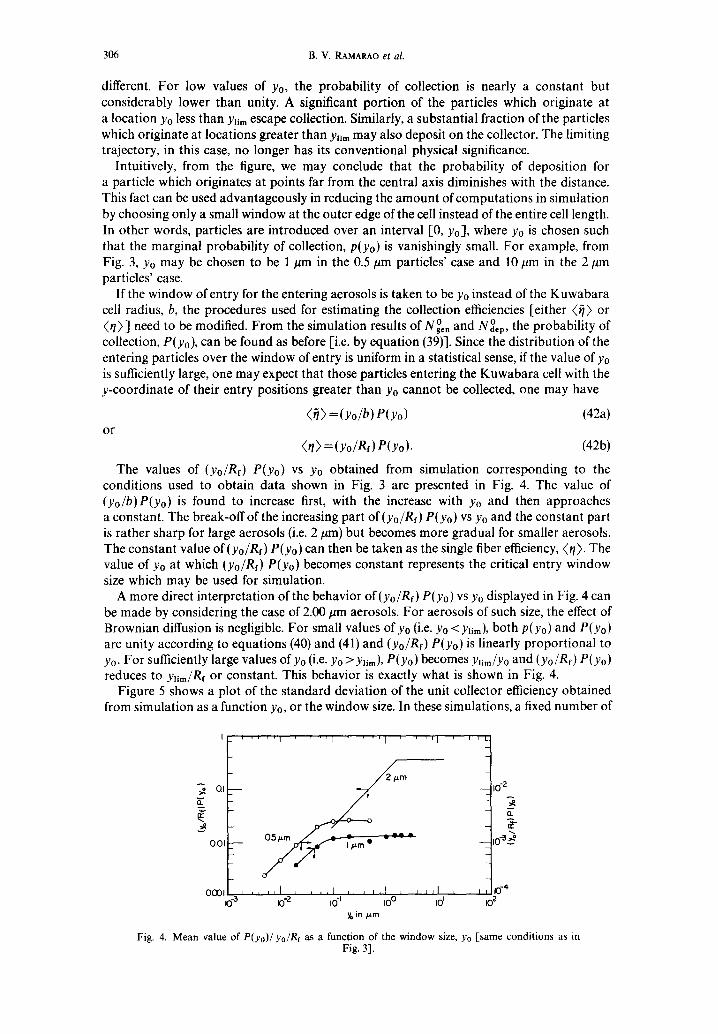
If the window of entry for the entering aerosols is taken to be Yo instead of the Kuwabara cell radius, b, the procedures used for estimating the collection efficiencies [either (~) or (r/)] need to be modified. From the simulation results of NO, and o Ndep, the probability of collection, P(Yo), can be found as before [i.e. by equation (39)]. Since the distribution of the entering particles over the window of entry is uniform in a statistical sense, if the value ofyo is sufficiently large, one may expect that those particles entering the Kuwabara cell with the y-coordinate of their entry positions greater than Yo cannot be collected, one may have
(~l) = (yo/b) e(yo) (42a) or
(rl) =(yo/Rf) P(Yo). (42b)
The values of (yo/Rf) P(Yo) vs Yo obtained from simulation corresponding to the conditions used to obtain data shown in Fig. 3 are presented in Fig. 4. The value of (yo/b)P(yo) is found to increase first, with the increase with Yo and then approaches a constant. The break-off of the increasing part of (yo/Rf) P(Yo) vs Yo and the constant part is rather sharp for large aerosols (i.e. 2 #m) but becomes more gradual for smaller aerosols. The constant value of(yo/Rf) P(Yo) can then be taken as the single fiber efficiency, (7). The value of Yo at which (yo/Rf) P(Yo) becomes constant represents the critical entry window size which may be used for simulation.
A more direct interpretation of the behavior of(yo/Re) P(Yo) vs Yo displayed in Fig. 4 can be made by considering the case of 2.00 #m aerosols. For aerosols of such size, the effect of Brownian diffusion is negligible. For small values of Yo (i.e. Yo <Y,m), both P(Yo) and P(Yo) are unity according to equations (40) and (41) and (yo/Rf) P(Yo) is linearly proportional to Yo- For sufficiently large values of Yo (i.e. Yo > Ylim), P(Yo) becomes Ylim/YO and (yo/Rf) P( Yo ) reduces to yl~m/Rf or constant. This behavior is exactly what is shown in Fig. 4.
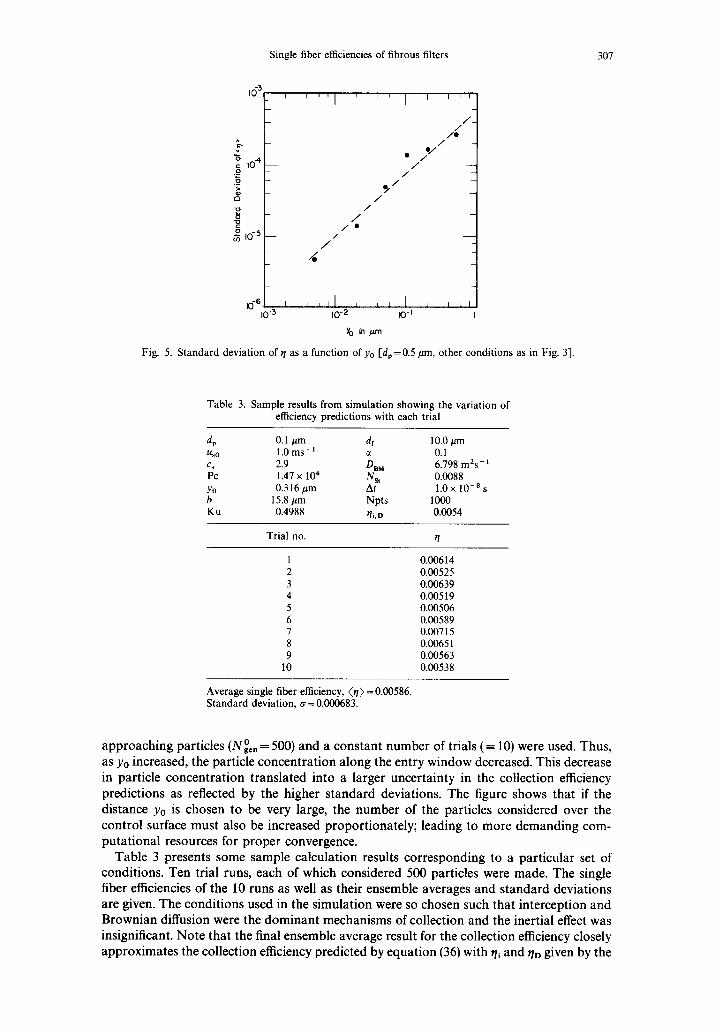
Figure 5 shows a plot of the standard deviation of the unit collector efficiency obtained from simulation as a function Yo, or the window size. In these simulations, a fixed number of
"~ O. I
0.01
. . . . . I . . . . I . . . . I ' ' l l
o,"
000110_3, , , j,l10 -2J ~ ,,110 -I , ,,110 ° ' y. in p.m
J J J l ~0 L
I i I - -
t~
f t .
I J ~0 " 4
~o 2
Fig. 4. Mean value of P(Yo)/yo/Rf as a function of the window size, Y0 [same conditions as in Fig. 31.
Single fiber efficiencies of fibrous filters 307
163
v "5 .0
g CI
o io 5 _
io -6 . I 10-3
I E i i I w
/ /
/ • /
/
I I I ~ I I 1 0 - 2
~b n ,~m
. / • / ]
/ /
/
I I I I I I I0-1
Fig. 5. Standard deviation of ~/as a function of Yo [dp=0.5/~m, other conditions as in Fig. 3].
Table 3. Sample results from simulation showing the variation of efficiency predictions with each trial
dp 0.1/~m df 10.0 #m us0 1.0 m s - ~ a 0.1 cs 2.9 DBM 6.798 mZs- 1 Pe 1.47 x 10⁴ Nst 0.0088 Yo 0.316 #m At 1.0 x 10 s s b 15.8/~m Npts 1000 Ku 0.4988 ~h,D 0.0054
Trial no.
1 0.00614 2 0.00525 3 0.00639 4 0.00519 5 0.00506 6 0.00589 7 0.00715 8 0.00651 9 0.00563
10 0.00538
Average single fiber efficiency, ( r / )=0.00586. Standard deviation, a=0.000683.
approaching particles (NOn = 500) and a constant number of trials ( = 10) were used. Thus, as Yo increased, the particle concentration along the entry window decreased. This decrease in particle concentration translated into a larger uncertainty in the collection efficiency predictions as reflected by the higher standard deviations. The figure shows that if the distance Yo is chosen to be very large, the number of the particles considered over the control surface must also be increased proportionately; leading to more demanding com- putational resources for proper convergence.
Table 3 presents some sample calculation results corresponding to a particular set of conditions. Ten trial runs, each of which considered 500 particles were made. The single fiber efficiencies of the 10 runs as well as their ensemble averages and standard deviations are given. The conditions used in the simulation were so chosen such that interception and Brownian diffusion were the dominant mechanisms of collection and the inertial effect was insignificant. Note that the final ensemble average result for the collection efficiency closely approximates the collection efficiency predicted by equation (36) with ~/i and r/D given by the
308 B.V. RAMARAO et al.
sum of equations (34) and (35), respectively. This indicates that in this region of the parameter space (viz. N~i and Npe), the principle of additivity is quite valid.
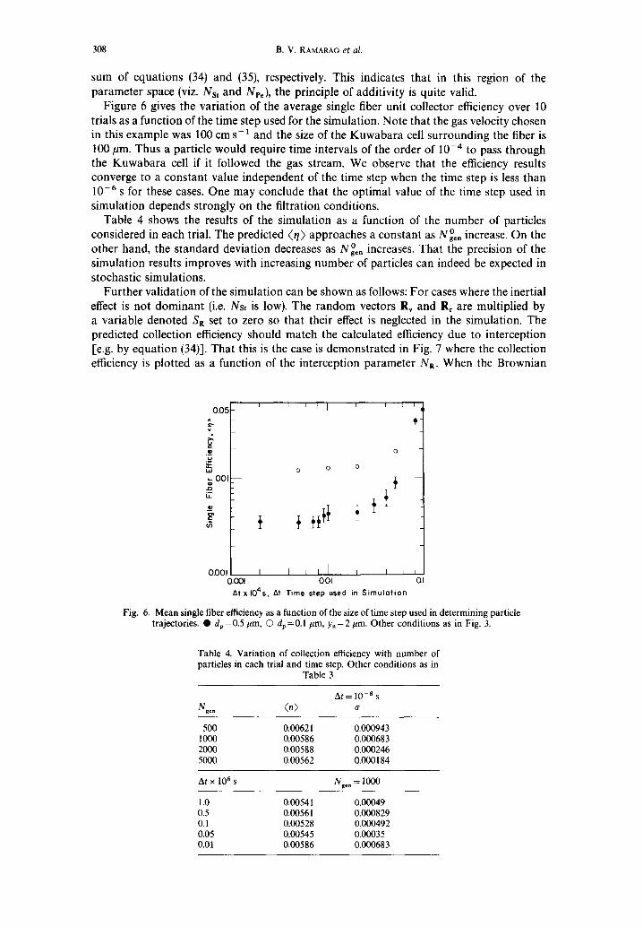
Figure 6 gives the variation of the average single fiber unit collector efficiency over 10 trials as a function of the time step used for the simulation. Note that the gas velocity chosen in this example was 100 cm s- 1 and the size of the Kuwabara cell surrounding the fiber is 100 #m. Thus a particle would require time intervals of the order of 10 -4 to pass through the Kuwabara cell if it followed the gas stream. We observe that the efficiency results converge to a constant value independent of the time step when the time step is less than 10 - 6 S for these cases. One may conclude that the optimal value of the time step used in simulation depends strongly on the filtration conditions.
Table 4 shows the results of the simulation as a function of the number of particles considered in each trial. The predicted (r/) approaches a constant as NOn increase. On the other hand, the standard deviation decreases as Ng°. increases. That the precision of the simulation results improves with increasing number of particles can indeed be expected in stochastic simulations.
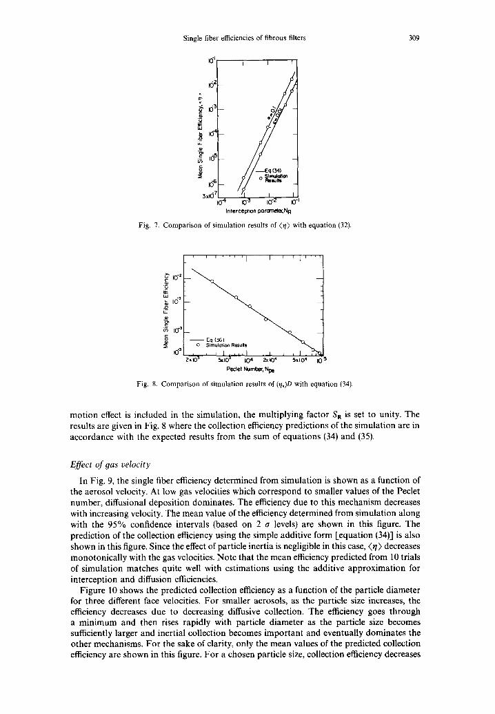
Further validation of the simulation can be shown as follows: For cases where the inertial effect is not dominant (i.e. Nst is low) . The random vectors Rv and R, are multiplied by a variable denoted SR set to zero so that their effect is neglected in the simulation. The predicted collection efficiency should match the calculated efficiency due to interception [e.g. by equation (34)-I. That this is the case is demonstrated in Fig. 7 where the collection efficiency is plotted as a function of the interception parameter NR. When the Brownian
00,'
v
~ O0
ft.
o . o o I
i i ' I I I
0 0
0
I I I I I I I I i ).o01 001 QI At x 1045, At Time step used in S imu la t ion
Fig. 6. Mean single fiber efficiency as a function of the size of time step used in determining particle trajectories. • dp=0.5 pm, © dp=0.1 pro, y , = 2 #m. Other conditions as in Fig. 3.
Table 4. Variation of collection efficiency with number of particles in each trial and time step. Other conditions as in
Table 3
At=10 as N o . ( , ) cr
500 0.00621 0.000943 1000 0.00586 0.000683 2000 0.00588 0.000246 5000 0.00562 0.000184
At x 106 s N g e . = 1000
1.0 0.00541 0.00049 0.5 0.00561 0.000829 0.1 0.00528 0.000492 0.05 0.00545 0.00035 0.01 0.00586 0.000683
Single fiber efficiencies of fibrous filters 309
I~l I t 1"
162 _ ^
"=' ~ 4 -
,~ - t o %
3xltJ 7 1.. 10-4 ~-3 10-2 iO-I
Interception po ron'~e, N R
Fig. 7. Comparison of simulat ion results of Q/ ) with equation (32).
" iO-z IQ LIJ
' 6 3
l u
b5 10 -3
{ g3
' ' I . . . . I I ' ' I ' "
O $imulotion Results
2xlO 3 ,~10 a 104 2xlO 4 5xIO* 10 5 Pet:let Number, Npe
Fig. 8. Comparison of simulation results of (r/s)D with equation {34).
motion effect is included in the simulation, the multiplying factor SR is set to unity. The results are given in Fig. 8 where the collection efficiency predictions of the simulation are in accordance with the expected results from the sum of equations (34) and (35).
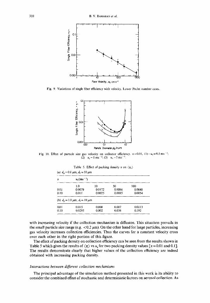
Effect of gas velocity
In Fig. 9, the single fiber efficiency determined from simulation is shown as a function of the aerosol velocity. At low gas velocities which correspond to smaller values of the Peclet number, diffusional deposition dominates. The efficiency due to this mechanism decreases with increasing velocity. The mean value of the efficiency determined from simulation along with the 95% confidence intervals (based on 2 a levels) are shown in this figure. The prediction of the collection efficiency using the simple additive form [equation (34)] is also shown in this figure. Since the effect of particle inertia is negligible in this case, Q/) decreases monotonically with the gas velocities. Note that the mean efficiency predicted from 10 trials of simulation matches quite well with estimations using the additive approximation for interception and diffusion efficiencies.
Figure 10 shows the predicted collection efficiency as a function of the particle diameter for three different face velocities. For smaller aerosols, as the particle size increases, the efficiency decreases due to decreasing diffusive collection. The efficiency goes through a minimum and then rises rapidly with particle diameter as the particle size becomes sufficiently larger and inertial collection becomes important and eventually dominates the other mechanisms. For the sake of clarity, only the mean values of the predicted collection efficiency are shown in this figure. For a chosen particle size, collection efficiency decreases
310 B.V. RAMARAO et al.
^
v
hi
L2
_e 0.01
O.OOI
0 .1 -
" 1 ' ' " 1 ' ' '
I0 I00 1003
Face Velocity, u s cm s q
Fig. 9. Variations of single fiber efficiency with velocity. Lower Peclet number cases.
QI i ^
.~ QOI -
0 .001 L
QOI
' ' ' 1 . . . . I
0.I 1.0 Particle Diameter, do in/~m
Fig. 10. Effect of particle size gas velocity on collector efficiency. ~=0.01, (l)~u~=0.5 ms-1; (2)~us = 1 ms-l; (3)--us =2 ms -1.
Table 5. Effect of packing density ~ on (rh)
(a) dp=0.1/am, df=10/~m
u~(ms-b
1.0 10 50 100 0.01 0,0079 0.0172 0.0086 0.0048 0.10 0,011 0.0025 0.0085 0.0054
(b) dp = 1.0/tm, dr= 10/am
0.01 0.015 0.008 0.007 0.0113 0.10 0.0295 0.002 0.036 0.192
with increasing velocity if the collection mechanism is diffusion. This situation prevails in the small particle size range (e.g. < 0.2 #m). On the other hand for large particles, increasing gas velocity increases collection efficiencies. Thus the curves for a constant velocity cross over each other in the right port ion of this figure.
The effect of packing density on collection efficiency can be seen from the results shown in Table 5 which gives the results of Q/) vs us for two packing density values [~ =0.01 and 0.1]. The results demonst ra te clearly that higher values of the collection efficiency are indeed obtained with increasing packing density.
Interactions between different collection mechanisms
The principal advantage of the simulation method presented in this work is its ability to consider the combined effect of stochastic and deterministic factors on aerosol collection. As
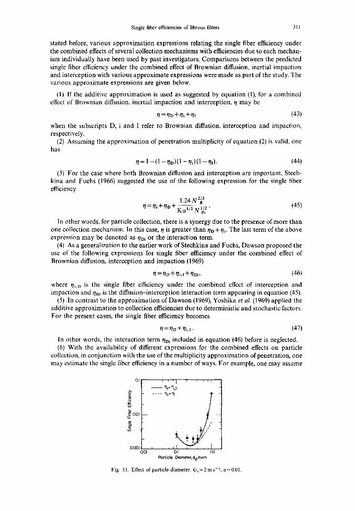
Single fiber efficiencies of fibrous filters 311
stated before, various approximation expressions relating the single fiber efficiency under the combined effects of several collection mechanisms with efficiencies due to each mechan- ism individually have been used by past investigators. Comparisons between the predicted single fiber efficiency under the combined effect of Brownian diffusion, inertial impaction and interception with various approximate expressions were made as part of the study. The various approximate expressions are given below.
(1) If the additive approximation is used as suggested by equation (1), for a combined effect of Brownian diffusion, inertial impaction and interception, ! /may be
/~ = I~D "]- ?]i + ~]I (43)
when the subscripts D, i and I refer to Brownian diffusion, interception and impaction, respectively.
(2) Assuming the approximation of penetration multiplicity of equation (2) is valid, one has
r/= 1 --(1 -- riD) (1 - r/i) (1 -r/i ). (44)
(3) For the case where both Brownian diffusion and interception are important, Stech- kina and Fuchs (1966) suggested the use of the following expression for the single fiber efficiency
1.24 N 2/s
q =r/i+r/D4 Kul/2 N pc 1/2" (45)
In other words, for particle collection, there is a synergy due to the presence of more than one collection mechanism. In this case, r/is greater than qo + qi. The last term of the above expression may be denoted as r/Di or the interaction term.
(4) As a generalization to the earlier work of Stechkina and Fuchs, Dawson proposed the use of the following expressions for single fiber efficiency under the combined effect of Brownian diffusion, interception and impaction (1969)
F / = 710 "~- ?]i.I + F/Oi, (46)
where r/i.o is the single fiber efficiency under the combined effect of interception and impaction and r/Di is the diffusion-interception interaction term appearing in equation (45).
(5) .In contrast to the approximation of Dawson (1969), Yoshika et al. (1969) applied the additive approximation to collection efficiencies due to deterministic and stochastic factors. For the present cases, the single fiber efficiency becomes
q = qD + r/i,l. (47)
In other words, the interaction term qDi included in equation (46) before is neglected. (6) With the availability of different expressions for the combined effects on particle
collection, in conjunction with the use of the multiplicity approximation of penetration, one may estimate the single fiber efficiency in a number of ways. For example, one may assume
0.1
0131 LU
0 . 0 0 1 0.01
. . . . I ' ' ' 1 - - ~o + ~ i , I
. . . . ~ o + tTl
i [ I t I i i 0 . I 1.0
P a r t i c l e D iome te r , dp i n p m
Fig. 11. Effect of particle diameter. Us= 2 m s- 1, ~ =0.01.
Tab
le
6.
Sin
gle
fibe
r ef
fici
ency
cal
cula
tion
s by
Bro
wni
an d
ynam
ics
sim
ulat
ion
com
pare
d to
eff
icie
ncy
pred
icti
ons
by o
ther
met
hods
Uso
~/
aD X
102
tr
ap x
10:
r/D
X 1
0 z
Fli, 1
×
102
(~/D
+rh)
10 z
(~D
'~-r
li,l
)10
2 E
quat
ion
(45)
E
quat
ion
(44)
E
quat
ion
(44)
E
quat
ion
(47)
Ns
, Nv
c x 1
0 -4
w
ith
th=
0
dr=
0.1/
zm
r/i-
-0.0
178
x 10
-2
r/x
102
100
0.52
9 0.
064
0.52
3 0.
0174
0.
541
0.54
1 0.
54
0.54
0.
558
0.59
0.
0085
1.
471
200
0.33
2 0.
092
0.32
9 0.
0174
0.
347
0.34
7 0.
377
0.34
7 0.
365
0.34
7 0.
0176
2.
942
300
0.24
61
0.02
8 0.
250
0.01
72
0.26
8 0.
267
0.28
8 0.
268
0.28
5 0.
268
0.02
64
4.41
3 50
0 0.
1897
0.
043
0.17
9 0.
0174
0.
197
0.19
7 0.
209
0.19
7 0.
215
0.19
7 0.
044
7.35
5 80
0 0.
1676
0.
033
0.13
1 0.
019
0.14
86
0.15
0.
154
0.15
0.
168
0.14
9 0.
070
4.76
8 10
00
0.17
02
0.03
3 0.
113
0.02
0 0.
1305
0.
133
0.13
4 0.
1507
0.
150
0.13
1 0.
088
14.7
1
d v =
0.2
gm
17
i =0.
0708
x 1
0 -2
100
0.38
9 0.
052
0.24
7 0.
067
0.31
77
0.31
4 0.
31
0.31
7 0.
383
0.31
4 0.
023
4.53
20
0 0.
263
0.06
3 0.
156
0.06
9 0.
226
0.22
5 0.
199
0.22
7 0.
295
0.22
5 0.
0457
9.
06
300
0.24
4 0.
043
0.11
87
0.08
0.
1895
0.
191
0.15
4 0.
198
0.26
7 0.
187
0.06
85
13.6
50
0 0.
264
0.06
3 0.
0844
0.
095
0.15
52
0.17
9 0.
116
0.1
64
0.25
9 0.
179
0.11
42
22.6
7 80
0 0.
364
0.06
6 0.
0617
0.
152
0.13
24
0.21
4 0.
083
0.14
1 0.
293
0.21
4 0.
183
36.2
6 10
00
0.51
4 0.
064
0.05
32
0.22
5 0.
1239
0.
278
0.07
2 0.
133
0.35
8 0.
278
0.22
84
45.3
3
dp=
0.3/
~m
~/
i =0.
157
× 10
-2
100
0.38
14
0.03
17
0.16
67
0.15
68
0.32
43
0.32
3 0.
226
0.32
4 0.
480
0.32
4 0.
043
8.17
20
0 0.
342
0.05
6 0.
105
0.18
34
0.26
26
0.28
9 0.
147
0.26
8 0.
444
0.28
8 0.
085
16.3
5 30
0 0.
389
0.05
3 0.
08
0.22
0.
237
0.30
0.
114
0.23
7 0.
456
0.29
9 0.
128
24.5
3 50
0 0.
590
0.01
3 0.
0570
0.
38
0.21
46
0.43
7 0.
083
0.21
4 0.
593
0.43
7 0.
214
40.8
9 80
0 5.
770
0.06
4 0.
0416
3.
58
0.19
9 3.
62
0.06
26
0.19
8 3.
77
3.62
0.
342
65.4
3 10
00
18.7
0 0.
29
0.03
59
16.4
0 0.
1936
16
.44
0.05
5 0.
193
16.6
16
.43
0.42
7 81
.78
> ~r
> > o
Single fiber efficiencies of fibrous filters 313
that
q = 1 --(1 -- qD) (1 -- ~]i,I)" (48)
The compar isons are shown in Fig. 11 and Table 6. In Fig. 11, the single fiber efficiency obtained from simulations, r/BD for u s = 2 m s -x and ct=0.01 is shown as a function of the particle diameter. Also included are the results of qD + qi and r/D + r/i.i. It is clear that as dp increases, the difference between qBD and qD+qi,I diminishes. On the other hand, for sufficiently small particles (dp~<0.1/~m), when the Brownian diffusion is the dominan t collection mechanism, the difference between these three values are negligible. For the in-between particle sizes, the additive approximat ion does not give accurate approximat ion no mat ter how this approximat ion is applied. This seems to suggest the presence of s t rong synergy between the deterministic and stochastic mechanisms.
A more extensive compar ison can be seen from the results tabulated in Table 6. The results given in this table include those shown in Fig. 11 as well as results according to equat ion (45) [with or without r/i], (44) and (47). It is clear that regardless whether the approximat ions were based on the additivity of simple fiber efficiencies due to individual mechanisms, or the multiplicity of penetrations, there exist significant differences between the Brownian dynamics simulation results and those according to the various approxima- tion. Simulation was found to give high collection efficiencies in the region where the min imum collection efficiency exists.
A possible explanat ion of this difference may be offered as follows. It is known from past studies (specifically, Fernandez de la M o r a and Rosner (1981, 1982)) that, in aerosol flow, particle inertia may cause an enhancement in particle concentrat ions in the front part of a cylindrical or spherical collector, which is referred to as inertial enrichment. As a conse- quence of this inertial enhancement in concentrat ion, there is a corresponding increase in particle flux (or collection efficiency) resulting from an increase in the driving force, (i.e. concentra t ion difference). That the Brownian dynamics simulation gives enhanced collec- tion efficiency as compared to additivity is indeed in agreement with this argument.
Acknowledgment~This work was conducted under subcontract B 160739 "Deposition of Diffusive Aerosols", Lawrence Livermore Laboratory, Livermore, CA. Support of the Empire State Paper Research Associates for this work is also gratefully acknowledged.
R E F E R E N C E S
Chandrasekhar, S. (1943) Rev. Mod. Phys. 15, 1. Davis, C. N. (1973) Air Filtration. Academic Press, London. Dawson, S. V. (1969) Sc.D. Thesis, Harvard Univ., Boston. Ermak, D. L. and McCammon, J. A. (1978). J. Chem. Phys. 69, 1352. Fernandez de la Mora, J. and Rosner, D. E. 0981) Physicochemical Hydrodynamics 2, I. Fernandez de la Mora, J. and Rosner, D. E. (1982) J. Fluid Mech. 125, 379. Friedlander, S. K. (1977) Smoke, Dust and Haze. Wiley, New York. Gupta, D. and Peters, M. H. 0985) J. Coll. Interf Sci. 104, 375. Gupta, D. and Peters, M. H. (1986) J. Coll. Interf Sci. 110, 286. IMSL Libraries 0985) IMSL, Inc., Houston, Texas. Kanaoka, C., Emi, H. and Tanthapanichakoon, W. (1983) AIChE J. 29, 845. Kasper, G., Preining, O. and Matteson, M. J. (1978) J. Aerosol Sci. 9, 331. Kuwabara, S. (1959) J. Phys. Soc. (Japan) 14, 527. Lee, K. W. and Liu, B. Y. H. (1982). Aerosol Sci. Technol. 1, 147. Liu, B. Y. H. and Rubow, K. K. (1986) Air Filtration by Fibrous Media, ASTM STP 973, Vol. 1. O'Brien, J. A. (1990) J. Coll. Interf Sci. 134, 497. Pich, J. (1987) Gas filtration theory. In Filtration Principles & Practices (Edited by Matteson, M. J. and Orr, C.) 2nd
Ed., Marcel-Dekker, New York. Ramarao, B. V. and Tien, C. (1991a) Simulation of particle deposition in fluid flow. In Transport Processes in
Bubbles, Drops and Particles (Edited by Chhabra, R. P. and DeKee, D.). Hemisphere Publishing Corp., New York. pp. 191-246.
Ramarao, B. V. and Tien, C. (1991b) J. Aerosol Sci. 21, 597~11. Stechkina, I. B. and Fuchs, N. A. (1966) Ann. Occup. Hy9. 9, 59. Tien, C. (1989) Granular Filtration of Aerosols and Hydrosols. Butterworths, New York. Yoshioka, N., Emi, H., Matsumura, H. and Yasunami, M. (1969) Kagaku Kogaku 33, 381 (in Japanese)(quoted by
Pith, 1979). Yuu, S. and Jotaki, T. (1978) Chem. Eng. Sci. 33, 971.