ALTERNATIVE FREQUENCY AND TIME DOMAIN VERSIONS OF FRACTIONAL BROWNIAN MOTION

Alternative Frequency and Time Domain Versions ofFractional Brownian Motion

James Davidson� and Nigar HashimzadeUniversity of Exeter

March 2006Forthcoming in Econometric Theory.

Abstract

This paper compares models of fractional processes and associated weak convergence re-sults based on moving average representations in the time domain with spectral representa-tions. Both approaches have been applied in the literature on fractional processes. We pointout that the conventional forms of these models are not equivalent, as is commonly assumed,even under a Gaussianity assumption. We show that it is necessary to distinguish between�two-sided�processes depending on both leads and lags from one-sided or �causal�processes,since in the case of fractional processes these models yield di¤erent limiting properties. Wederive new representations of fractional Brownian motion, and show how di¤erent results areobtained for, in particular, the distribution of stochastic integrals in the multivariate con-text. Our results have implications for valid statistical inference in fractional integration andcointegration models.

�Corresponding author, [email protected]. We thank F. Hashimzade and two anonymous refereesfor their valuable comments.

1

1 Introduction

Two approaches to studying the asymptotics of long memory, fractional integration and cointe-gration models have been developed in recent literature. In the �rst of these, which we call the�time domain moving average�model, the fractionally integrated process is commonly written as

xt = (1� L)�dut (1.1)

where L represents the lag operator, jdj < 12 , and ut is a short memory (weakly dependent)

process. As is well known, the binomial expansion of (1�L)�d yields the in�nite moving averagerepresentation

xt =1Xj=0

bjut�j

where

bj =�(d+ j)

�(d)�(j + 1):

and �() denotes the gamma function. Under the indicated restriction on d the lag coe¢ cients aresquare summable, and the process is accordingly covariance stationary. In many applications weconsider the linear case where

ut = �(L)"t

with f"tg i.i.d.(0; �2) and �(L) =P1l=0 �jL

j , having absolutely summable coe¢ cients. See, forexample, Granger and Joyeux (1980), Hosking (1981), Beran (1994) and many related references.

In the second approach, the frequency domain harmonizable representation of the process isadopted. De�ne

xt =

Z �

��eit�h(ei�)W (d�) (1.2)

where i is the imaginary unit and W is a complex-valued Gaussian random measure with theproperties

W (�d�) =W (d�) (1.3a)

E(W (d�)) = 0 (1.3b)

E(W (d�)W (d�)) =

��2d�; � = �0; otherwise

(1.3c)

Observe that xt is always real-valued since the integrals over [��; 0] and [0; �] are complexconjugates. h(ei�) is called the transfer function or frequency response function of the process.If xt is i.i.d. then h(ei�) = 1=

p2� (constant), but otherwise we wish to think of it at this stage

merely as some function of �, complex-valued in general, to be speci�ed by the context. It ishowever related to the spectral density of the process by f(�) = �2

��h(ei�)��2, and in the longmemory case the latter function is often represented in the generic form

f(�) = j�j�2dL(�)

where d matches the parameter in (1.1), and L(�) is at most slowly varying at 0.1 See Robinson(1994b), Brockwell and Davis (1991) Section 13.2, among other references, for further details ofthis type of model. Note that the harmonizable representation is more specialized than the time

1Here, L() is the standard generic notation for a slowly varying function, not to be confused with the lagoperator L.

2

domain model since it requires the process to be Gaussian and stationary, whereas ut in (1.1) canbelong to a more general class of processes. However, these models are often treated, explicitlyor implicitly, as being merely alternative representations of the same process. A key feature ofthe theory is that the associated normalized partial-sum processes should converge weakly to aGaussian a.s.-continuous limit process known as fractional Brownian motion (fBM).

The object of this paper is to show that there are, in fact, important di¤erences between thesemodels as commonly represented, and that, in particular, alternative versions of the fractionalmodel lead to di¤erent limit processes. The di¤erences are not trivial, and may have completelydi¤erent implications for joint distributions in the multivariate case. Section 2 describes a classof harmonizable representations of fractional Brownian motion, all sharing a common spectrumapart from scale constants, and shows how they can be derived as the weak limits of forwardand/or backward-looking linear moving average processes. Section 3 considers the multivariatecase, and examines the cross-spectra and covariance functions of di¤erent members of the class.Section 4 considers the distribution of the stochastic integral of one process with respect tothe increments of another, and generalizations of Chan and Terrin�s (1995) weak convergenceresults are proved. Section 5 presents a complementary analysis of time domain representations,generalizing the model �rst proposed by Mandelbrot and van Ness (1968), and gives a generalizedweak convergence result for this class using the approach of Davidson and de Jong (2000). Finally,Section 6 discusses our results in the context of the existing literature, and shows how they resolvea number of puzzles and contradictory features of this literature. Proofs are gathered in theAppendix.

2 Harmonizable Representations of Fractional Brownian Motion

In this section we introduce a class of continuous time Gaussian processes,

X(r; d; �; a) =1p2�

Z 1

�1

ei�r � 1i�

~g(�; d; �; a)W (d�) (2.1)

where W is a complex-valued Gaussian process on R satisfying the conditions of (1.3), and ~g isa complex valued transfer function having the general form

~g(�; d; �; a) = � (i�)a�d (�i�)�a + (1� �) (i�)�a (�i�)a�d : (2.2)

for real constants d; �; a, where �12 � d <

12 , 0 � a � d=2 for d > 0 and d=2 � a � 0 for d < 0,

and 0 � � � 1.We mention two points of clari�cation at the outset. The �rst is to emphasize that this model

class is introduced as a vehicle for developing and illustrating the representation issues addressedin the paper. We do not attempt to assign any particular interpretation to the parameters � anda which, as we show, can be thought of as indexing di¤erent distributed lead/lag structures. Wewill, in fact, argue that most practical applications in econometrics are covered by one particularcase (see (2.8) below). Second, note that in the sequel we use the generic notation X(r) to denoteany member of the class, so that dependence on the three parameters is taken as implicit. Thisis chie�y for notational clarity, since the expressions involving several coordinates of X wouldotherwise become unwieldy.

Now, note the identity

(�i�)s = (�i sgn(�))s j�js = exp��i sgn(�)s�

2

�j�js

where sgn(�) = 1 if � � 0 and �1 otherwise. Thus, (2.2) can also be written as

~g(�; d; �; a) = j�j�d�(�; d; �; a) (2.3)

3

where

�(�; d; �; a) = � exp (�i� (d=2� a) sgn(�)) + (1� �) exp (i� (d=2� a) sgn(�)) : (2.4)

Further note that

j�(�; d; �; a)j2 = 1� 4�(1� �) sin2 ��d

2� a�

= K(d; �; a)2 (2.5)

(de�ning K(d; �; a)) and so the generalized spectral densities of this class of processes take theform

j~g(�; d; �; a)j2 = j�j�2dK(d; �; a)2:Alternatively, the variance of a process increment of width � > 0, for any r 2 [0; 1� �], is

E(X(r + �)�X(r))2

=1

2�E

Z 1

�1

ei�(r+�) � ei�ri�

~g(�; d; �; a)W (d�)

�Z 1

�1

ei�(r+�) � ei�ri�

~g(�; d; �; a)W (d�)

=�2

2�K(d; �; a)22

Z 1

�1(1� cos��)j�j�2d�2d�

=�2K(d; �; a)2

�(2d+ 2) cos�d�2d+1 (2.6)

where the last equality can be veri�ed from Gradshteyn and Ryzhik (2000) (henceforth GR)Relation 3.823. Applying the identity

(X(r4)�X(r3))(X(r2)�X(r1)) = 12 [(X(r4)�X(r1))

2 + (X(r3)�X(r2))2

� (X(r3)�X(r1))2 � (X(r4)�X(r2))2]: (2.7)

for any r1; r2; r3; r4 2 [0; 1] with r1 < r2 and r3 < r4, formula (2.6) can be used to derive thecovariance of any pair of segments of the process. The covariance structure of these processestherefore depends on a and � only through the scale factor K(d; �; a), and otherwise matchesthat of what is usually called �fractional Brownian motion�. Since in general �2 is unknown, theseparameters are accordingly unidenti�ed from the point of view of a single process.

Any of these processes are candidates to be referred to as fractional Brownian motion, andsome leading examples of the class have been proposed in the literature. Setting � = 1 and a = 0yields

X(r) =1p2�

Z 1

�1

ei�r � 1i�

(i�)�dW (d�) (2.8)

(See e.g. Reed, Lee and Truong 1995). Setting a = d=2 on the other hand (in which case � dropsout) yields

X(r) =1p2�

Z 1

�1

ei�r � 1i�

j�j�dW (d�) (2.9)

which, apart from an at most slowly varying component, is the model examined extensively byChan and Terrin (1995). As a further variant, set � = 1

2 and a = 0 to yield

X(r) =1p2�

Z 1

�1

ei�r � 1i�

Re(i�)�dW (d�): (2.10)

4

The last case has not been proposed to date, to our knowledge, but provides an alternative to(2.9) as a way of representing symmetry of the backward and forward-looking dependence. Aswe show, this property is implicit in any model having a real-valued transfer function.

As noted, Chan and Terrin (1995), in common with other contributions to this literature,allow slowly varying components in the transfer function and spectral density. Our class ofmodels might easily be elaborated to include, for example, a slowly varying, even function of �as a factor in (2.3). Such extensions would complicate the analysis, but would not change thebasic conclusions. While these issues would be of interest to explore further, we choose to focusthe present discussion on the model as given.

One way to to motivate our class is by considering a corresponding class of discrete processesin the time domain. We may then show how the Brownian motions derived above can be viewedas weak limits as the time intervals shrink to zero. Let

ut =1p2�

Z �

��ei�tW (d�)

represent a serially independent Gaussian process with mean 0 and variance �2, and so considera �two-sided�moving average process

xt = g(L; d; �; a)ut =1X

j=�1bjut�j (2.11)

whereg(L; d; �; a) = �(1� L)a�d(1� L�1)�a + (1� �)(1� L)�a(1� L�1)a�d: (2.12)

It is easily veri�ed that the lag structure is a convolution of the binomial series associated withfractional integration. Thus,

b0 =1

�(a)�(d� a)

1Xk=0

�(a+ k)�(d� a+ k)�(k + 1)2

;

bj =1

�(a)�(d� a)

1Xk=0

��(a+ k)�(d� a+ k + j) + (1� �)�(d� a+ k)�(a+ k + j)

�(k + 1)�(k + j + 1)

�;

b�j =1

�(d� a)�(a)

1Xk=0

��(d� a+ k)�(a+ k + j) + (1� �)�(a+ k)�(d� a+ k + j)

�(k + 1)�(k + j + 1)

�for j > 0. Note that

1Xk=0

�(a+ k)�(d� a+ k + j)�(k + 1)�(k + j + 1)

�1Xk=0

ka�1(j + k)d�a�1

= jd�2jXk=0

�k

j

�a�1�1 +

k

j

�d�a�1+

1Xk=j+1

kd�2�j

k+ 1

�d�a�1� Ajd�1

for 0 < A <1, and similarly1Xk=0

�(d� a+ k)�(a+ k + j)�(k + 1)�(k + j + 1)

�1Xk=0

kd�a�1(j + k)a�1 � Ajd�1:

5

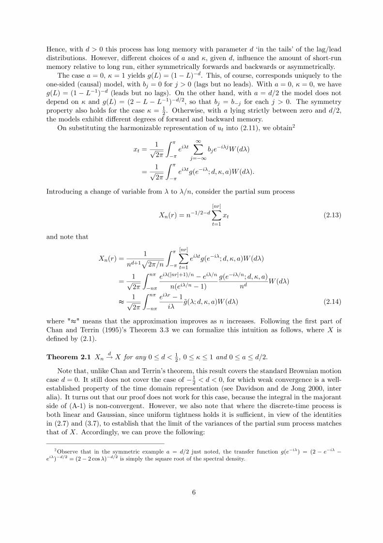
Hence, with d > 0 this process has long memory with parameter d �in the tails�of the lag/leaddistributions. However, di¤erent choices of a and �, given d, in�uence the amount of short-runmemory relative to long run, either symmetrically forwards and backwards or asymmetrically.

The case a = 0, � = 1 yields g(L) = (1� L)�d. This, of course, corresponds uniquely to theone-sided (causal) model, with bj = 0 for j > 0 (lags but no leads). With a = 0, � = 0, we haveg(L) = (1 � L�1)�d (leads but no lags). On the other hand, with a = d=2 the model does notdepend on � and g(L) = (2 � L � L�1)�d=2, so that bj = b�j for each j > 0. The symmetryproperty also holds for the case � = 1

2 . Otherwise, with a lying strictly between zero and d=2,the models exhibit di¤erent degrees of forward and backward memory.

On substituting the harmonizable representation of ut into (2.11), we obtain2

xt =1p2�

Z �

��ei�t

1Xj=�1

bje�i�jW (d�)

=1p2�

Z �

��ei�tg(e�i�; d; �; a)W (d�):

Introducing a change of variable from � to �=n, consider the partial sum process

Xn(r) = n�1=2�d

[nr]Xt=1

xt (2.13)

and note that

Xn(r) =1

nd+1p2�=n

Z �

��

[nr]Xt=1

ei�tg(e�i�; d; �; a)W (d�)

=1p2�

Z n�

�n�

ei�([nr]+1)=n � ei�=n

n(ei�=n � 1)g(e�i�=n; d; �; a)

ndW (d�)

t1p2�

Z n�

�n�

ei�r � 1i�

~g(�; d; �; a)W (d�) (2.14)

where "t" means that the approximation improves as n increases. Following the �rst part ofChan and Terrin (1995)�s Theorem 3.3 we can formalize this intuition as follows, where X isde�ned by (2.1).

Theorem 2.1 Xnd! X for any 0 � d < 1

2 , 0 � � � 1 and 0 � a � d=2:

Note that, unlike Chan and Terrin�s theorem, this result covers the standard Brownian motioncase d = 0. It still does not cover the case of �1

2 < d < 0, for which weak convergence is a well-established property of the time domain representation (see Davidson and de Jong 2000, interalia). It turns out that our proof does not work for this case, because the integral in the majorantside of (A-1) is non-convergent. However, we also note that where the discrete-time process isboth linear and Gaussian, since uniform tightness holds it is su¢ cient, in view of the identitiesin (2.7) and (3.7), to establish that the limit of the variances of the partial sum process matchesthat of X. Accordingly, we can prove the following:

2Observe that in the symmetric example a = d=2 just noted, the transfer function g(e�i�) = (2 � e�i� �ei�)�d=2 = (2� 2 cos�)�d=2 is simply the square root of the spectral density.

6

Theorem 2.2 If

xt =1p2�

Z �

��ei�t

�1� e�i�

��dW (d�)

for �12 < d <

12 , and Xn(r) is de�ned by (2.13), then Xn

d! X where X(r) is de�ned by (2.8).

While this statement of the result is given only for the causal member of our class having � = 1and a = 0, note that both the �nite-n and limiting variance expressions are generalized to thecases with 0 � � � 1 and d=2 � a � 0 simply by applying the factor K(d; �; a)2. The result maybe easily extended in this way to our complete class of Gaussian linear processes.

3 The Multivariate Case

It is clear that all processes xt de�ned by (2.11) have the same spectral density function, andaccordingly the limiting partial sum processes have the same autocovariance structure, the oneusually identi�ed with �fractional Brownian motion�. However, it is also the case that theseprocesses are distinct, and we now consider how they might be distinguished. This can only bein terms of the relations between di¤erent processes.

Consider processes X1 and X2 de�ned as in (2.1) with parameters (d1; �1; a1) and (d2; �2; a2)and driving processes W1, W2. The latter are complex-valued Gaussian random measures withthe properties (for j; k = 1; 2)

Wj(�d�) =Wj(d�) (3.1a)

EWj(d�) = 0 (3.1b)

EWj(d�)Wk(d�) =

��jkd�; � = �0; otherwise.

(3.1c)

In this section and the one following we let 0 � dj < 12 for j = 1; 2 We do not attempt to treat

the cases dj < 0 explicitly, although we conjecture that these extensions might be developed onthe lines of Theorem 2.2.

De�ne

P12(�) = �(�; d1; �1; a1)�(��; d2; �2; a2):

=4Xj=1

�j exp(i��j sgn(�)) (3.2)

where

�1 = �1�2; �1 = ��a1 � a2 �

d1 � d22

��2 = (1� �1) (1� �2) ; �2 = a1 � a2 �

d1 � d22

�3 = �1 (1� �2) ; �3 = ��a1 + a2 �

d1 + d22

��4 = (1� �1)�2 �4 = a1 + a2 �

d1 + d22

Observe, from (2.1), that the cross-spectrum of the increments is de�ned as

f12(�) = ~g(�; d; �; a)~g(��; d2; �2; a2)= j�j�d1�d2P12(�):

7

We can notice, for example, that f12(�) is real-valued in the �time symmetric� cases, whereeither a1 = d1=2 and a2 = d2=2, or �1 = �2 =

12 , although not in general. However, we

can potentially learn more by considering time-domain covariances of the Brownian motions,extending the formulation in (2.6).

Consider the case of contemporaneous increments.

Proposition 3.1 For � > 0 and 0 � r � 1� �,

E[(X2 (r + �)�X2 (r)) (X1 (r + �)�X1 (r))]

=�12�

d1+d2+1

� (2 + d1 + d2) cos�d1 + d22

�cos�

�a1 � a2 �

d1 � d22

��

2 [�1 (1� �2) + (1� �1)�2] sin��a1 �

d12

�sin�

�a2 �

d22

��(3.3)

Note that this formula reduces to (2.6) in the case X1 = X2 = X: We cannot use it to derive thecovariances of non-coincident increments of the two processes, since there is no counterpart toidentity (2.7). However, for the case of non-overlapping increments the following can be showndirectly.

Proposition 3.2 For 0 � r1 < r2 � r3 < r4 � 1,

(i) If d1 + d2 > 0,

E[(X2 (r4)�X2 (r3)) (X1 (r2)�X1 (r1))]

=�12U (d1; d2)

� (d1 + d2 + 2) sin� (d1 + d2)

4Xj=1

�j sin�

�d1 + d22

� �j�

(3.4)

where

U(d1; d2) = (r4 � r1)d1+d2+1 � (r4 � r2)d1+d2+1 � (r3 � r1)d1+d2+1 + (r3 � r2)d1+d2+1 (3.5)

(ii) If d1 = d2 = 0,E[(X2(r4)�X2(r3))(X1(r2)�X1(r1))] = 0: (3.6)

To deal with the case r2 > r3, such that the increments are overlapping, this result may be usedin conjunction with (3.3) and the identity

(X2(r4)�X2(r3))(X1(r2)�X1(r1)) = (X2(r4)�X2(r2))(X1(r2)�X1(r1))+ (X2(r2)�X2(r3))(X1(r2)�X1(r3))

+ (X2(r2)�X2(r3))(X1(r3)�X1(r1)): (3.7)

Consider, for example, the case of non-overlapping segments where X1 is a backward-lookingprocess, with �1 = 1 and a1 = 0, and X2 a forward-looking process, with �2 = 0 and a2 = 0. Inthis case �1 = �2 = �4 = 0, and �3 =

12(d1 + d2), hence (3.4) vanishes, as we should expect since

the lags and leads do not overlap anywhere. However, if �2 = 1 and �1 = 0, so that the segmentof the forward-looking process on r2 � r1 precedes the segment of the backward-looking processon r4 � r3, then �1 = �2 = �3 = 0, and the expression in (3.6) reduces to

E[(X2(r4)�X2(r3))(X1(r2)�X1(r1))] =�12U(d1; d2)

� (2 + d1 + d2)

8

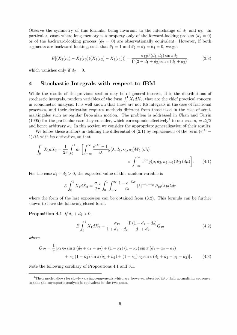
Observe the symmetry of this formula, being invariant to the interchange of d1 and d2. Inparticular, cases where long memory is a property only of the forward-looking process (d1 = 0)or of the backward-looking process (d2 = 0) are observationally equivalent. However, if bothsegments are backward looking, such that �1 = 1 and �2 = �3 = �4 = 0, we get

E[(X2(r4)�X2(r3))(X1(r2)�X1(r1))] =�12U(d1; d2) sin�d2

� (2 + d1 + d2) sin� (d1 + d2): (3.8)

which vanishes only if d2 = 0:

4 Stochastic Integrals with respect to fBM

While the results of the previous section may be of general interest, it is the distributions ofstochastic integrals, random variables of the form

R 10 X1dX2, that are the chief practical concern

in econometric analysis. It is well known that these are not Itô integrals in the case of fractionalprocesses, and their derivation requires methods di¤erent from those used in the case of semi-martingales such as regular Brownian motion. The problem is addressed in Chan and Terrin(1995) for the particular case they consider, which corresponds e¤ectively3 to our case ai = di=2and hence arbitrary �i. In this section we consider the appropriate generalization of their results.

We follow these authors in de�ning the di¤erential of (2.1) by replacement of the term (ei�r�1)=i� with its derivative, so thatZ 1

0X1dX2 =

1

2�

Z 1

0dr

�Z 1

�1

ei�r � 1i�

~g(�; d1; �1; a1)W1 (d�)

�Z 1

�1ei�r~g(�; d2; �2; a2)W2 (d�)

�: (4.1)

For the case d1 + d2 > 0, the expected value of this random variable is

E

Z 1

0X1dX2 =

�122�

Z 1

0

Z 1

�1

1� e�i�ri�

j�j�d1�d2 P12(�)d�dr

where the form of the last expression can be obtained from (3.2). This formula can be furthershown to have the following closed form.

Proposition 4.1 If d1 + d2 > 0;

E

Z 1

0X1dX2 =

�121 + d1 + d2

� (1� d1 � d2)d1 + d2

Q12 (4.2)

where

Q12 =1

�[�1�2 sin� (d2 + a1 � a2) + (1� �1) (1� �2) sin� (d1 + a2 � a1)

+ �1 (1� �2) sin� (a1 + a2) + (1� �1)�2 sin� (d1 + d2 � a1 � a2)] : (4.3)

Note the following corollary of Propositions 4.1 and 3.1.

3Their model allows for slowly varying components which are, however, absorbed into their normalizing sequence,so that the asymptotic analysis is equivalent in the two cases.

9

Corollary 4.1 If d1 + d2 > 0,

E

�Z 1

0X1dX2 +

Z 1

0X2dX1

�= E(X1(1)X2(1)): (4.4)

Also note that the case d1 = d2 = 0 has to be excluded from these results because our formulain (4.2) then reduces to

E

Z 1

0X1dX2 =

�122+�122�

Z 1

0

Z 1

�1

sin2 �r

i�d�dr: (4.5)

Although its integrand is an odd function, the integral on the right-hand side has the form1�1,so that the expectation is unde�ned.

Now consider some contrasting cases of (4.2). We obtain the last term of Chan and Terrin�sformula (3.11), apart from scale factor, by setting aj = dj=2 with arbitrary �j , for j = 1; 2. Inthis case we obtain the closed form

E

Z 1

0X1dX2 =

�12� (1� d1 � d2)�(1 + d1 + d2)(d1 + d2)

sin�

�d2 + d12

�.

A feature of this model, consequent on the forward-backward symmetry of the lag structure, isthat the formula is symmetric in d1 and d2. We are not able to distinguish between the case oflonger-memory integrand with shorter-memory integrator and the converse case.

In the case of the causal model, in which �1 = �2 = 1 and a1 = a2 = 0, on the other hand,we obtain

E

Z 1

0X1dX2 =

�12� (1� d1 � d2)�(1 + d1 + d2)(d1 + d2)

sin�d2:

Note, in a result that parallels (3.8), how this quantity vanishes when d2 = 0, although not whend1 = 0.

We next proceed to generalize the second part of Chan and Terrin�s Theorem 3.3, whichestablishes weak convergence of the stochastic integral. Letting x1t, x2t be de�ned like (2.11)with parameters (dj ; �j ; aj) for j = 1; 2; our result is as follows.

Theorem 4.1 If 0 � d1 < 12 , 0 � d2 <

12 and d1 + d2 > 0 then

X1n; X2n;n�1�d1�d2

n�1Xt=1

tXs=1

x1sx2;t+1

!d!�X1; X2;

Z 1

0X1dX2

�: (4.6)

Observe that our conditions here are weaker than the min(d1; d2) > 0 imposed by Chan andTerrin, permitting cases where either of X1 and X2 are standard Brownian motions. However, thecase d1 = d2 = 0 is again problematic, not withstanding that the conditions for mean-squaredconvergence established in the theorem are still satis�ed. This follows from the fact noted in(4.5), that the limit speci�ed by formula (4.1) is not an integrable random variable.

The problem arising here can be seen to stem from the approximation of the extreme high-frequency components implicit in the Fourier transformation. This approximation is negligible inthe long memory case thanks to non-summability of the autocovariances. In standard Brownianmotions, however, it is well known that the equality in (4.4) requires an additional term �12on the left-hand side, representing the contemporaneous correlation of the processes. It is alsowell known that replacing the partial sum

Pts=1 x1s = S1t in (4.6) by 1

2(S1t + S1;t+1) yields

10

the Stratonovich integral4 having expectation 12�12, under mean-square convergence in the time

domain, instead of the Itô integral having expectation 0. By contrast, an easy implication ofour proof is that the limit de�ned by (4.1) is invariant to �nite lead-lag shifts of the integrandsequence in (4.6).

5 Variants of Fractional Brownian Motion in the Time Domain

Let B denote Brownian motion on R with variance E[B(1)�B(0)]2 = �2. The Gaussian stochasticprocess on the unit interval [0; 1] with representation

X(r) =1

�(d+ 1)

�Z r

0(r � s)ddB(s) +

Z 0

�1[(r � s)d � (�s)d]dB(s)

�(5.1)

was termed fractional Brownian motion (fBM) by Mandelbrot and van Ness (1968). Robinson andMarinucci (1999) have subsequently dubbed this process fractional Brownian motion of Type I, incontrast with the Type II case in which the second term is discarded. Type II fBM is sometimesrationalized as the weak limit of a process in which the forcing sequence takes the truncatedform utI(t � 1). However, it�s important to note that the resulting weak limit has a di¤erentdistribution, and is not to be regarded as an approximation to (5.1).

It is well known (see for example Davidson and de Jong 2000) that the increment variance ofType I fBM is de�ned by

E[X(r + �)�X(r)]2 = V �2d+1

where

V = E(X(1)2) =�2

�(d+ 1)2

�1

2d+ 1+

Z 1

0[(� + 1)d � �d]2d�

�=

�2�(1� 2d)(2d+ 1)�(1� d)�(1 + d) : (5.2)

The second equality in (5.2) is a consequence of the following lemma, whose proof we give, forthe record, in the Appendix.

Lemma 5.1Z 1

0[(� + 1)d � �d]2d� = 1

2d+ 1

��(1� 2d)�(1 + d)

�(1� d) � 1�:

In this section, we extend this time domain representation to a class of the processes whoseharmonizable representation is discussed in Section 2. To be precise, we consider just the caseswith 0 � � � 1 and a = 0, since for these the extension of (5.1) is simple and transparent. Let

X(r) =

Z r

0[�(r � s)d + (1� �)sd]dB(s) + �

Z 0

�1[(r � s)d � (�s)d]dB(s)

+ (1� �)Z 1

r[sd � (s� r)d]dB(s); 0 � r � 1: (5.3)

De�ning the �ltration

F = fF(r) = �(B(s); s � r);�1 < r <1g

note that (X;F) are an adapted pair in the case � = 1, which corresponds to (5.1). This isanother way to express the notion of a causal process. Otherwise, X is F(1)-measurable at all

4See, inter alia, Duncan, Hu and Pasik Duncan (2000).

11

points, and hence not adapted to F : With � = 12 , such that the forward and backward looking

moving averages are symmetric, note that this model corresponds to case (2.10), while with � = 1it corresponds to (2.8).

We remark parenthetically that there appears no natural way to de�ne a �Type II�variant ofthis class of model. Thus, the process fX(r), 0 � r � 1g obtained by deleting the second and thirdterms of (5.3) corresponds to the weak limit of a fractionally integrated process whose forcingsequence takes the form utI(1 � t � [nr]) for each r. One could truncate the forcing sequence atn and hence the third integral at 1, instead of deleting it, but this option foregoes the bene�ts ofsimplicity and seems equally arbitrary. There are many ways to construct stochastic processeshaving correlated increments, subject to a parameter d, but not all of them have relevance toeconometric modelling.

The next proposition derives the general formula for the increment variances.

Proposition 5.1 E[X(r + �)�X(r)]2 = V �2d+1 where

V =�2

�(1 + d)(2d+ 1)

�2�(1� �) �(1 + d)

�(1 + 2d)+ (1� 2�(1� �))�(1� 2d)

�(1� d)

�:

We need to check the relationship between this formula and (2.6) obtained in the harmonizablerepresentation for the case a = 0: The following proposition shows they are identical.

Proposition 5.2 V =�2K(d; �; 0)2

� (2d+ 2) cos�d:

The main implication to be remarked here is that the Mandelbrot-Van Ness model (5.1) is shownto be equivalent to the causal variant (2.8) of the harmonizable representation, these beingGaussian processes with identical covariance structure. This fact may suggest a further needfor caution in adopting the Type II variant of time domain fBM in the causal model. Hav-ing nonstationary increments, the Type II variant evidently does not possess a harmonizablerepresentation.

Since empirical processes will always be subject to an unknown scale factor �, it is notpossible to distinguish the processes represented by (5.3) from one another in isolation, and �is unidenti�ed. However, similar arguments allow us to show that for processes X1 and X2 thecovariances of process segments, and E

R 10 X1dX2, depend on �1; �2. This can be veri�ed simply

by considering the harmonizable representations in Sections 3 and 4, which yield equivalentformulae.

It is known (Davidson and de Jong 2000, Theorem 3.1) that if xt = (1� L)�dut, where futgsatis�es fairly weak regularity conditions and

Xn(r) = n�1=2�d

[nt]Xt=1

xt (5.4)

then Xnd! X where X is de�ned by (5.1), and d! here denotes weak convergence in the space

D[0;1] of cadlag functions on the unit interval, equipped with the Skorokhod topology (see, e.g.,Davidson 1994, Ch. 28). We can now extend this result as follows.

Theorem 5.1 Ifxt = [�(1� L)�d + (1� �)(1� L�1)�d]ut

for any d 2 (�12 ;12) and � 2 [0; 1]; and Xn is de�ned in (5.4), then Xn

d! X under the assump-tions on ut speci�ed by Davidson and de Jong�s (2000) Theorem 3.1.

12

We refer the reader to the cited source for details of the speci�ed conditions, which are quitecomplicated to state. It su¢ ces to say that they specify weak dependence in the form of L2-near-epoch dependence on a mixing process, at speci�ed sizes. These conditions are invariantto time reversal, which allows the extension of the results speci�ed in the proof of the presentproposition. Also note that this proposition is not redundant in view of Theorem 2.1, not merelybecause it covers the cases d < 0; but because it allows a very general class of weakly dependentshock processes. While it is possible to introduce additional weak dependence in Theorem 2.1(we avoid this for the sake of simplicity) note that Gaussianity is a necessary condition, in thespectral approach.

6 Discussion

In the literature on fractional Brownian motion, there is a tendency to assume the existence of asingle Gaussian process having the characteristics of interest. In the time domain, the formulationmost often cited is the one of Mandelbrot and van Ness (1968). Among many references in theengineering, statistics and econometrics literature see Flandrin (1989), Samorodnitsky and Taqqu(1994, Sect. 7.2), Read, Lee and Truong (1995).

However, there is less consensus regarding the so-called harmonizable representation of frac-tional Brownian motion. Samorodnitsky and Taqqu (1994, Sect. 7.2), which is, perhaps, the chiefreference source on these topics, refers to one of the �time-symmetric�members of our class, thathaving a = d=2 and arbitrary �, as the (integral representation of) �standard�fractional Brown-ian motion, and Chan and Terrin (1995) follow suit. On the other hand, Reed et al. (1995)cite the �causal�form (� = 1; a = 0). Kim and Phillips (2001) actually cite the causal versionin the statement of their model, but then switch to the time symmetric case in their working,while following the Chan-Terrin analysis. This apparent confusion is very likely attendant on thefact that the underlying stationary driving processes all have the same spectrum. Indeed, Chanand Terrin (1995) explicitly set up their model by citing the spectral density of interest (j�j1�2Hmultiplied by a possibly slowly varying scale component), and then selecting the square root ofthis function as the transfer function to de�ne their harmonizable representation.

However, as we have shown in this paper, the Mandelbrot-Van Ness time domain modeland the time-symmetric model discussed by Samorodnitsky-Taqqu, Chan-Terrin and other au-thors, have very di¤erent implications for multivariate analysis, despite the stationary incrementprocesses sharing the same spectrum, apart from scale constants. We note that Chan-Terrininvoke econometric applications explicitly in their introduction, introduce a unit root autore-gressive (backward-looking) model, and even quote the one-sided time domain representation(1� L)dyt to motivate their formal analysis of the long memory errors. This suggests that theydid not fully appreciate the modelling implications of their chosen harmonizable representation.When the applications of interest are in time series econometrics, we ought to point out that formost applications only a single member of our class should generally be considered; the causal(i.e. exclusively backward-looking) Mandelbrot-Van Ness model, with harmonizable representa-tion (2.8) having � = 1, a = 0 in the Gaussian case. Time-series processes in econometrics arealmost always thought of as adapted to the �ltration representing �events to present date�, sinceany other setup would contradict our usual understanding of economic behaviour. 5

Frequency-domain analysis is a popular research methodology in time series econometrics,especially in the analysis of long memory and fractional integration and cointegration. We cancite for example the many contributions of Peter Robinson and co-authors; Robinson (1994a,b),

5Two-sided models could have applications in random �eld representations involving spatial correlations, forexample.

13

Robinson and Marinucci (2001, 2003), Marinucci and Robinson (1999, 2000, 2001) is a non-exhaustive list covering just one aspect of this research. One obvious motivation for this method-ology is the greater mathematical tractability often available in the asymptotic analysis of longmemory models. By the same token, however, we see a need to emphasize the potential pitfallsof modelling dynamic relationships in a framework that may conceal the important role of causalorderings.

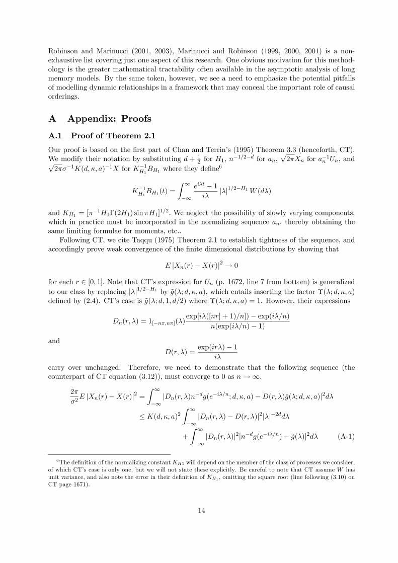
A Appendix: Proofs

A.1 Proof of Theorem 2.1

Our proof is based on the �rst part of Chan and Terrin�s (1995) Theorem 3.3 (henceforth, CT).We modify their notation by substituting d + 1

2 for H1, n�1=2�d for an,

p2�Xn for a�1n Un, andp

2��1K(d; �; a)�1X for K�1H1BH1 where they de�ne

6

K�1H1BH1(t) =

Z 1

�1

ei�t � 1i�

j�j1=2�H1W (d�)

and KH1 = [��1H1�(2H1) sin�H1]1=2: We neglect the possibility of slowly varying components,

which in practice must be incorporated in the normalizing sequence an, thereby obtaining thesame limiting formulae for moments, etc..

Following CT, we cite Taqqu (1975) Theorem 2.1 to establish tightness of the sequence, andaccordingly prove weak convergence of the �nite dimensional distributions by showing that

E jXn(r)�X(r)j2 ! 0

for each r 2 [0; 1]: Note that CT�s expression for Un (p. 1672, line 7 from bottom) is generalizedto our class by replacing j�j1=2�H1 by ~g(�; d; �; a), which entails inserting the factor �(�; d; �; a)de�ned by (2.4). CT�s case is ~g(�; d; 1; d=2) where �(�; d; �; a) = 1. However, their expressions

Dn(r; �) = 1[�n�;n�](�)exp[i�([nr] + 1)=n])� exp(i�=n)

n(exp(i�=n)� 1)

and

D(r; �) =exp(ir�)� 1

i�

carry over unchanged. Therefore, we need to demonstrate that the following sequence (thecounterpart of CT equation (3.12)), must converge to 0 as n!1:

2�

�2E jXn(r)�X(r)j2 =

Z 1

�1jDn(r; �)n�dg(e�i�=n; d; �; a)�D(r; �)~g(�; d; �; a)j2d�

� K(d; �; a)2Z 1

�1jDn(r; �)�D(r; �)j2j�j�2dd�

+

Z 1

�1jDn(r; �)j2jn�dg(e�i�=n)� ~g(�)j2d� (A-1)

6The de�nition of the normalizing constant KH1 will depend on the member of the class of processes we consider,of which CT�s case is only one, but we will not state these explicitly. Be careful to note that CT assume W hasunit variance, and also note the error in their de�nition of KH1 , omitting the square root (line following (3.10) onCT page 1671).

14

Since Dn(r; �) ! D(r; �) pointwise on [0; 1] � R, to show the �rst majorant term vanishes itsu¢ ces to show thatZ 1

�1jDn(r; �)j2j�j�2dd� =

Z �n

��njDn(r; �)j2j�j�2dd� <1:

uniformly in n. Note �rst that

jDn(r; �)j2 = 1[�n�;n�]��exp [i� ([nr] + 1) =n]� exp (i�=n)n (exp (i�=n)� 1)

��2= 1[�n�;n�]

jexp [i� ([nr] + 1) =n]� exp (i�=n)j2

jn (exp (i�=n)� 1)j2

= 1[�n�;n�]1

n2(exp [i� ([nr] + 1) =n]� exp (i�=n)) (exp [i� ([nr] + 1) =n]� exp (i�=n))

(exp (i�=n)� 1) (exp (�i�=n)� 1)

= 1[�n�;n�]1

n22� 2 cos� [nr] =n2� 2 cos�=n

= 1[�n�;n�]1

n2sin2 � [nr] =2n

sin2 �=2n:

Therefore, using the resultssin2 kx

sin2 x� k2 (A-2)

and Z �=2

0

sin2 kx

sin2 xdx =

�k

2(A-3)

for integer k � 0, observe thatZ �n

��njDn(r; �)j2j�j�2dd� =

Z �n

��n

1

n2sin2 � [nr] =2n

sin2 �=2nj�j�2dd�

= 2

Z �n

0

1

n2sin2 � [nr] =2n

sin2 �=2n��2dd�

= 2

�Z 1

0

1

n2sin2 � [nr] =2n

sin2 �=2n��2dd�+

Z �n

1

1

n2sin2 � [nr] =2n


�� 2

Z 1

0

[nr]2

n2��2dd�+

Z �n

1

1

n2sin2 � [nr] =2n


!

� 2�

1

1� 2d +Z �n

1

1

n2sin2 � [nr] =2n


�� 2

�1

1� 2d +Z �n

0

sin2 � [nr] =2n

sin2 �=2nd�

�= 2

�1

1� 2d +1

n22n�

2[nr]

�� 2

�1

1� 2d + ��: (A-4)

To show that the second majorant term in (A-1) vanishes as n!1, note that

jn�dg(e�i�=n)� ~g(�)j2

15

=��[(i�+O(n�1))a�d(�i�+O(n�1))�a � (i�)a�d(�i�)�a]

+(1� �)[(i�+O(n�1))�a(�i�+O(n�1))a�d � (i�)�a(�i�)a�d]��2 : (A-5)

Taking the �rst right-hand side term under the modulus in (A-5), note that

(i�+O(n�1))a�d(�i�+O(n�1))�a � (i�)a�d(�i�)�a = j�j�d$1n(�; a; d):

where

$1n(�; a; d) = [(ei� sgn(�)=2 +O(n�1))a�d(e�i� sgn(�)=2 +O(n�1))�a � e�i�(d=2�a) sgn(�)]

= O(n�1): (A-6)

The same treatment of the second right-hand side term yields an expression$2n(�; a; d) = O(n�1)similarly. Note that $1n(�; a; d) and $2n(�; a; d) depend on � only through its sign, and hencethe squared modulus in (A-5) depends on � only through j�j�2d:We therefore complete the proofby applying (A-4) as before.


We show that E[Xn (r)2] ! E[X (r)2] for each r 2 [0; 1]. As remarked in the text, this condition

is su¢ cient for the weak convergence, since the sequence members are linear and Gaussian foreach n � 1 and uniform tightness holds as before, by appeal to Taqqu (1975 Th. 2.1).

The spectral representation of Xn (r) is

Xn (r) =1

n1=2+d

[nr]Xt=1

1p2�

Z �

��ei�t

�1� e�i�

��dW (d�)

=1

n1=2+dp2�

Z �

��

[nr]Xt=1

ei�t�1� e�i�

��dW (d�)

=1

n1=2+dp2�

Z �

��ei�ei�[nr] � 1ei� � 1

�1� e�i�

��dW (d�)

=1

n1=2+dp2�

Z �

��

�ei�[nr] � 1

��1� e�i�

��d�1W (d�) :

The integrand can be rewritten as�ei�[nr] � 1

��1� e�i�

��d�1= ei�[nr]=22i sin

� [nr]

2

�e�i�=22i sin

�

2

��d�1= 2�dei�([nr]+d+1)=2 (i sgn�)�d sin

j�j [nr]2

sin�d�1j�j2

= 2�dei�([nr]+d+1)=2e�i sgn��d=2 sinj�j [nr]2

sin�d�1j�j2

The variance of Xn (r) is therefore equal to

Vn (r) =�2

2�

21�2d

n1+2d

Z �

0sin2

� [nr]

2sin�2d�2

�

2d�

16

=�2

2�

21�2d

n1+2d

Z �=2

02 sin2 ' [nr] sin�2d�2 'd'

=�2

2�

21�2d

n1+2d

Z �=2

0(1� cos 2' [nr]) sin�2d�2 'd':

By GR Relation 3.621(1),Z �=2

0sin�2d�2 'd' = 2�2d�3B

��d� 1

2;�d� 1

2

�=

�d

2d+ 1

� (1� 2d)[� (1� d)]2

where the second equality follows after some manipulation using the properties of the gammafunction. Next,Z �=2

0cos 2' [nr] sin�2d�2 'd' =

Z �=2

0cos 2

��2� '

�[nr] cos�2d�2 'd'

=

Z �=2

0cos (� [nr]� 2 [nr]') cos�2d�2 'd'

= (�1)[nr]Z �=2

0cos (2 [nr]') cos�2d�2 'd'

= (�1)[nr] �

2�2d�1 (�2d� 1)1

B (�d+ [nr] ;�d� [nr])

= � 22d

2d+ 1

�

cos�d

� (1 + d+ [nr])

� (1 + 2d) � (�d+ [nr])

where the penultimate equality follows from GR Relation 3.631(9). Upon substitution of theseexpressions into the expression for the variance we obtain

Vn (r) =�2

2�

21�2d

n1+2d

��d� (1� 2d)

(2d+ 1) [� (1� d)]2+

22d

2d+ 1

�

cos�d

� (1 + d+ [nr])

� (1 + 2d) � (�d+ [nr])

�:

In the limit, as n ! 1, the contribution of the �rst term in the brackets vanishes. For thesecond term we use

limn!1

� (1 + d+ [nr])

� (�d+ [nr]) [nr]�2d�1 = 1:

Hence,

limn!1

Vn (r) =�2

� (2 + 2d) cos�dr2d+1:

The right-hand side is equal to the variance of the fBM process

X (r) =1p2�

Z 1

�1

ei�r � 1i�

(i�)�dW (d�) :

To show this observe that the integrand can be rewritten as

ei�r � 1i�

(i�)�d = ei�r=22i sin�r

2(i�)�d�1

= 2ei�r=2 sinj�j r2j�j�d�1 (isgn�)�d

17

= 2ei�r=2e�isgn��d=2 sinj�j2j�j�d ;

and, hence, the variance of X (r) takes the form

V (r) =2�2

�

Z 1

�1sin2

j�j r2j�j�2d�2 d�

=2�2

�

Z 1

0(1� cos�r)��2d�2d�

=�2

� (2 + 2d) cos�dr2d+1

where the last equality follows from GR Relation 3.823.

A.3 Proof of Proposition 3.1

E[(X2 (r + �)�X2 (r))(X1 (r + �)�X1 (r))]

=�12�

Z 1

�1j�j�d1�d2�2 (1� cos��)P12(�) d�

=�12�

d1+d2+1

�

Z 1

�1jxj�d1�d2�2 (1� cosx)P12(x)dx: (A-7)

Substituting from (3.2), note that the last integral has four terms, with typical formZ 1

�1jxj�d1�d2�2 (1� cosx) ei��jsgn(x) dx = 2 cos��j

Z 1

0dx1� cosxx2+d1+d2

= 2 cos��j� csc �2 (d1 + d2 + 1)

2� (2 + d1 + d2)

=�

� (2 + d1 + d2)

cos��j

cos�d1 + d22

: (A-8)

(see GR, relations 3.761 and 3.823). Direct substitution into (A-7) gives (3.3).


E[(X2 (r4)�X2 (r3)) (X1 (r2)�X1 (r1))]

=�122�

Z 1

�1

ei�r4 � ei�r3i�

eg (�; d2; �2; a2) e�i�r2 � e�i�r1�i� eg (��; d1; �1; a1) d�=�122�

Z 1

�1j�j�d1�d2�2

�ei�r4 � ei�r3

��e�i�r2 � e�i�r1

�P12(�)d�:

Rearranging the terms with the exponents gives�ei�r4 � ei�r3

��e�i�r2 � e�i�r1

�= ei�(r4+r3)=2e�i�(r2+r1)=2

�ei�(r4�r3)=2 � e�i�(r4�r3)=2

��e�i�(r2�r1)=2 � ei�(r2�r1)=2

�= 4ei�[(r4+r3)�(r2+r1)]=2 sin�

r4 � r32

sin�r2 � r12

:

18

Next, de�ne integrals

�1 =

Z 1

0

d�

�d1+d2+2cos�

(r4 + r3)� (r2 + r1)2

sin�r4 � r32

sin�r2 � r12

�2 =

Z 1

0

d�

�d1+d2+2sin�

(r4 + r3)� (r2 + r1)2

sin�r4 � r32

sin�r2 � r12

and note that

�1 + i�2 =

Z 1

0

ei�[(r4+r3)�(r2+r1)]=2

�d1+d2+2sin�

r4 � r32

sin�r2 � r12

d�:

The expression for the covariance can accordingly be rewritten as

E[(X2 (r4)�X2 (r3))(X1 (r2)�X1 (r1))]

=2�12�

4Xj=1

�j

Z 1

�1

ei��j sgn(�)ei�[(r4+r3)�(r2+r1)]=2

j�jd1+d2+2sin�

r4 � r32

sin�r2 � r12

d�

=2�12�

4Xj=1

�j

hei��j (�1 + i�2) + e

�i��j (�1 � i�2)i

=4�12�

4Xj=1

�j��1 cos��j � �2 sin��j

�(A-9)

The integrand in �1 can be rearranged using a trigonometric identity as

cos�(r4 + r3)� (r2 + r1)

2sin�

r4 � r32

sin�r2 � r12

=1

2sin�

�r4 �

r2 + r12

�sin�

r2 � r12

� 12sin�

�r3 �

r2 + r12

�sin�

r2 � r12

:

Applying GR Relation 3.762(1) then yields

�1 =� sec�

d1 + d22

8� (d1 + d2 + 2)U (d1; d2)

where U (d1; d2) is given by (3.5). Note that �1 = 0 for d1 + d2 = 0.For �2, use GR Relations 3.763(1) and (3) to obtain

�2 =

8>>>>>>><>>>>>>>:

� csc�d1 + d22

8� (d1 + d2 + 2)U (d1; d2) ; d1 + d2 > 0;

1

4[(r4 � r1) ln (r4 � r1)� (r4 � r2) ln (r4 � r2)

+ (r3 � r1) ln (r3 � r1)� (r3 � r2) ln (r3 � r2)] ;d1 + d2 = 0:

Substituting these results in (A-9) yields (3.4) for the case d1 + d2 > 0. The case d1 = d2 = 0implies a1 = a2 = 0: Hence, �j = 0 for j = 1; 2; 3; 4 and

E [(X2 (r4)�X2 (r3)) (X1 (r2)�X1 (r1))] = �4�12�2�

4Xj=1

�j sin��j

= 0.

19


Since 0 6 r 6 1 we have sgn(�) = sgn(�r), and making the change of variables x = �r we canintegrate with respect to r independently. This yields the general formula

E

Z 1

0X1dX2 =

�122�

Z 1

0dr rd1+d2

Z 1

�1

1� e�ixix

jxj�d1�d2 P12(x)dx

=�122�

1

1 + d1 + d2

Z 1

�1

1� e�ixix

jxj�d1�d2 P12(x)dx (A-10)

where P12 is de�ned in (3.2), containing terms of the type exp�i��j sgn(�)

�, where �j is one

of the indicated functions of d1; d2; a1; a2. For any such term we can rewrite the correspondingcomponent of the integral over the real line in (A-10) (say, C(�j)), as

C(�j) �Z 1

�1dx1� e�ixix

jxj�d1�d2 exp�i��j sgn(�)

�=

Z 1

0dx1� e�ixix

jxj�d1�d2 exp�i��j

�+

Z 0

�1dx1� e�ixix

jxj�d1�d2 exp��i��j

�=

Z 1

0dx1� e�ixix

x�d1�d2 exp�i��j

�+

Z 1

0dx1� e�ix�ix x�d1�d2 exp

��i��j

�= J exp

�i��j

�+ J exp

��i��j

�(A-11)

where (�) denotes complex conjugation and

J =

Z 1

0dx

1� e�ixix1+d1+d2

=

Z 1

0dx1� cosx+ i sinx

ix1+d1+d2

= �iZ 1

0dx1� cosxx1+d1+d2

+

Z 1

0dx

sinx

x1+d1+d2

=�

2� (1 + d1 + d2)

h�i csc �

2(d1 + d2) + sec

�

2(d1 + d2)

i=

�

� (1 + d1 + d2)

�i exp�i�2 (d1 + d2)

�sin� (d1 + d2)

: (A-12)

Using (A-12) in (A-11),

C(�j) =�

� (1 + d1 + d2)

�ihexp

�i��d1+d22 + �j

�� exp

��i�

�d1+d22 + �j

��isin� (d1 + d2)

=2�

� (1 + d1 + d2)

sin��d1+d22 + �j

�sin� (d1 + d2)

and

E

Z 1

0X1dX2 =

�122�

1

1 + d1 + d2

4Xj=1

�jC(�j)

=�12

1 + d1 + d2

1

� (1 + d1 + d2)

1

sin� (d1 + d2)

4Xj=1

�j sin�

�d1 + d22

+ �j

�

=�12

1 + d1 + d2

� (d1 + d2)

� (1 + d1 + d2)

� (1� d1 � d2)�

4Xj=1

�j sin�

�d1 + d22

+ �j

�

20

=�12

1 + d1 + d2

� (1� d1 � d2)(d1 + d2)

1

�

4Xj=1

�j sin�

�d1 + d22

+ �j

�=

�121 + d1 + d2

� (1� d1 � d2)(d1 + d2)

Q12

where

Q12 =1

�

4Xj=1

�j sin�

�d1 + d22

+ �j

�and direct substitution yields (4.3).

A.6 Proof of Corollary 4.1

Note that E(X1(1)X2(1)) is given by setting � = 1 in (3.3). We show that this formula matchesthe sum of (4.2) and the complementary expression having 1 and 2 interchanged. First note,using the relations

� (1 + x) = x� (x) ; � (x) � (1� x) = �

sin�x;

that

1

� (2 + d1 + d2)=

1

1 + d1 + d2

1

� (1 + d1 + d2)

=1

1 + d1 + d2

� (1� d1 � d2)d1 + d2

1

� (d1 + d2) � (1� d1 � d2)

=1

1 + d1 + d2

� (1� d1 � d2)d1 + d2

sin� (d1 + d2)

�

Next, from (4.3), using that fact that

�1�2 + (1� �1) (1� �2) = 1� �1 (1� �2)� (1� �1)�2

and also the trigonometric identities

sin�+ sin� = 2 sin�+ �

2cos

�� 2

cos�� cos� = �2 sin �+ �2

sin�� 2

sin� = 2 sin�

2cos

�

2;

we complete the proof by noting

Q12 +Q21 =1

�[(�1�2 + (1� �1) (1� �2)) (sin� (d2 + a1 � a2) + sin� (d1 + a2 � a1))

+ (�1 (1� �2) + (1� �1)�2) (sin� (a1 + a2) + sin� (d1 + d2 � a1 � a2))]

=2

�sin�

d1 + d22

�cos�

�a1 � a2 �

d1 � d22

�� (�1 (1� �2) + (1� �1)�2)

��cos�

�a1 � a2 �

d1 � d22

�� cos�

�a1 + a2 �

d1 + d22

��=1

�

sin� (d1 + d2)

cos�d1 + d22

�cos�

�a1 � a2 �

d1 � d22

�

21

� 2 (�1 (1� �2) + (1� �1)�2) sin��a1 �

d12

�sin�

�a2 �

d22

��:


Following Chan and Terrin (1995, page 1674) de�ne

Bn(�; �) = 1[�n�;n�]2(�; �)1

n

n�1Xt=1

exp(i(t+ 1)�=n)� exp(i�=n)n(exp(i�=n)� 1) exp

�i(t+ 1)�

n

�and

B(�; �) =

Z 1

0exp(ir�)

exp(ir�)� 1i�

dr:

We prove, analogous to (3.14) of Chan and Terrin (1995), thatZ 1

�1

Z 1

�1jBn(�; �)n�d1�d2g1(e�i�=n)g2(e�i�=n)�B(�; �)~g1(�)~g2(�)j2d�d�! 0

as n!1: Note thatZ 1

�1

Z 1

�1jBn(�; �)n�d1�d2g1(e�i�=n)g2(e�i�=n)�B(�; �)~g1(�)~g2(�)j2d�d�

� K21K

22

Z 1

�1

Z 1

�1jBn(�; �)�B(�; �)j2j�j�2d1 j�j�2d2d�d�

+

Z 1

�1

Z 1

�1jBn(�; �)j2j�n(�; �)j2j�j�2d1 j�j�2d2d�d�: (A-13)

where ~gi(�) = ~g(�; di; �i; ai), gi(L) = g(L; di; �i; ai) and Ki = K(di; �i; ai), for i = 1; 2, and

�n(�; �) = 1[�n�;n�]2(�; �)�j�jd1 j�jd2(n�d1�d2g1(e�i�=n)g2(e�i�=n)� ~g1(�)~g2(�))

�: (A-14)

The factor 1[�n�;n�]2(�; �) can be optionally included in (A-14) since it does not change the valueof the integral in (A-13).

It is required to show that both the terms on the majorant of (A-13) converge to 0. It is easyto see that Bn (�; �) � B (�; �) ! 0 pointwise in R2, so in respect of the �rst term it su¢ ces toshow that Z 1

�1

Z 1

�1jBn(�; �)j2j�j�d1 j�j�d2d�d� <1

uniformly in n.At points inside [��n; �n]� [��n; �n],

jBn (�; �)j2 =n�1Xk=1

1

n

exp (i� (k + 1) =n)� exp (i�=n)n (exp (i�=n)� 1) exp (i� (k + 1) =n)

�n�1Xj=1

1

n

exp (�i� (j + 1) =n)� exp (�i�=n)n (exp (�i�=n)� 1) exp (�i� (j + 1) =n)

= Vn(�) + Sn (�; �) + Sn (�; �) (A-15)

where

Vn(�) =n�1Xk=1

1

n2jexp (i� (k + 1) =n)� exp (i�=n)j2

n2 j(exp (i�=n)� 1)j2=1

n4

n�1Xk=1

�sin (�k=(2n))

sin (�=(2n))

�2;

22

Sn =

n�1Xk=2

k�1Xj=1

1

n2[exp (i� (k + 1) =n)� exp (i�=n)] [exp (�i� (j + 1) =n)� exp (�i�=n)]

n2 (exp (i�=n)� 1) (exp (�i�=n)� 1)

� exp (i� (k � j) =n)

=n�1Xk=2

k�1Xj=1

1

n4exp (i� (k � j) =n)� exp (�i�j=n)� exp (i�k=n) + 1

(exp (i�=n)� 1) (exp (�i�=n)� 1) exp (i� (k � j) =n)

and Sn is the complex conjugate of Sn. Consider the last two terms in (A-15). Note thatZ �n

��n

Z �n

��n

�Sn + Sn

�j�j�2d1 j�j�2d2 d�d�

=1

n2

n�1Xk=2

k�1Xj=1

"Z �n

��nexp (i� (k � j) =n) d�

j�j2d2

�Z �n

��n

exp (i� (k � j) =n)� exp (�i�j=n)� exp (i�k=n) + 1n2 (exp (i�=n)� 1) (exp (�i�=n)� 1)

d�

j�j2d1

+

Z �n

��nexp (�i� (k � j) =n) d�

j�j2d2

�Z �n

��n

exp (�i� (k � j) =n)� exp (i�j=n)� exp (�i�k=n) + 1n2 (exp (i�=n)� 1) (exp (�i�=n)� 1)

d�

j�j2d1

#

=1

n2

n�1Xk=2

k�1Xj=1

"Z �n

��nexp (i� (k � j) =n) d�

j�j2d2

�Z �n

��n

exp (i� (k � j) =n)� exp (�i�j=n)� exp (i�k=n) + 1n2 (exp (i�=n)� 1) (exp (�i�=n)� 1)

d�

j�j2d1

+

Z �n

��nexp (i� (k � j) =n) d�

j�j2d2

�Z �n

��n

exp (�i� (k � j) =n)� exp (i�j=n)� exp (�i�k=n) + 1n2 (exp (i�=n)� 1) (exp (�i�=n)� 1)

d�

j�j2d1

#

=1

n2

n�1Xk=2

k�1Xj=1

Z �n

��ncos

� (k � j)n

d�

j�j2d2

�Z �n

��n

2 (1 + cos (� (k � j) =n)� cos (�j=n)� cos (�k=n))2 (1� cos (�=n))

d�

j�j2d1

=4

n2

n�1Xk=2

k�1Xj=1

Z �n

0cos

� (k � j)n

d�

�2d2

�Z �n

0

sin2 (�j=(2n)) + sin2 (�k=(2n))� sin2 (� (k � j) =(2n))n2 sin2 (�=(2n))

d�

�2d1

(A-16)

where in the second equality we did a change of variable from � to �� and in the third wecollected terms and cancelled odd components.

Consider �rst the integral with respect to �.Z �n

0cos

� (k � j)n

d�

�2d2=

Z 1

0cos

� (k � j)n

d�

�2d2+

Z �n

1cos

� (k � j)n

d�

�2d2

23

�Z 1

0

d�

�2d2+

Z �n

1cos

� (k � j)n

d�

=1

1� 2d2� sin (k � j) =n

(k � j) =n

� 1

1� 2d2� 1

using

��sinxx�� 1: Next consider the integral with respect to �. Using (A-2) and (A-3) we haveZ �n

0

sin2 (�j=(2n)) + sin2 (�k=(2n))� sin2 (� (k � j) =(2n))n2 sin2 (�=(2n))

d�

�2d1

�Z 1

0

sin2 (�j=(2n)) + sin2 (�k=(2n)) + sin2 (� (k � j) =(2n))n2 sin2 (�=(2n))

d�

�2d1

+

Z �n

1


d�

�2d1

�Z 1

0

1

n2

�j2 + k2 + (k � j)2

� d�

�2d1

+

Z �n

0


d�

�Z 1

06d�

�2d1+2n

n2� (j + k + (k � j))

� 6

1� 2d1+ 4�:

Substituting these bounds in (A-16) yieldsZ �n

��n

Z �n

��n

�Sn + Sn

�j�j�2d1 j�j�2d2 d�d� � 4

�1

1� 2d2+ 1

��6

1� 2d1+ 4�

�:

Next, considering the �rst term in (A-15), note thatZ �n

��n

Z �n

��nVn (�) j�j�2d1 j�j�2d2 d�d�

=1

n

Z �n

��nj�j�2d2 d� 1

n3

n�1Xk=1

Z �n

��n

sin2 (�k=(2n))

sin2 (�=(2n))j�j�2d1 d�

=4

n

Z �n

0��2d2d�

1

n3

n�1Xk=1

Z �n

0

sin2 (�k=(2n))

sin2 (�=(2n))��2d1d�

=4�

1�2d2

1� 2d2n�2d2

1

n3

n�1Xk=1

�Z 1

0

sin2 (�k=(2n))

sin2 (�=(2n))��2d1d�+

Z �n

1

sin2 (�k=(2n))

sin2 (�=(2n))��2d1d�

�

� 4�1�2d2

1� 2d2n�2d2

1

n3

n�1Xk=1

�Z 1

0k2��2d1d�+

Z �n

1

sin2 (�k=(2n))

sin2 (�=(2n))d�

�

� 4�1�2d2

1� 2d2n�2d2

1

n3

n�1Xk=1

�n2

1� 2d1+

Z �n

0

sin2 (�k=(2n))

sin2 (�=(2n))d�

�

=4�

1�2d2

1� 2d2n�2d2

1

n3

n�1Xk=1

�n2

1� 2d1+ 2n

�k

2

�

24

� 4�1�2d2

1� 2d2n�2d2

1

n3

n�1Xk=1

�n2

1� 2d1+ n2�

�

� 4�1�2d2

1� 2d2n�2d2

�1

1� 2d1+ �

�� 4�

1�2d2

1� 2d2

�1

1� 2d1+ �

�<1:

Observe that this term vanishes for d2 > 0, although not for d2 = 0.The same argument can be invoked again to show that the second majorant term of (A-13)

vanishes, provided �n(�; �) is bounded uniformly in n; and converges to 0 pointwise in R2. Toshow this, recall that

~g1(�)~g2(�) = j�j�d1 j�j�d2�(�; d1; �1; a1)�(�; d2; �2; a2)

where

�(�; d1; �1; a1)�(�; d2; �2; a2)

= �1�2e�i�[(d1=2�a1) sgn(�)+(d2=2�a2) sgn(�)]

+ (1� �1) (1� �2) ei�[(d1=2�a1) sgn(�)+(d2=2�a2) sgn(�)]

+ �1 (1� �2) e�i�[(d1=2�a1) sgn(�)�(d2=2�a2) sgn(�)]

+ (1� �1)�2ei�[(d1=2�a1) sgn(�)�(d2=2�a2) sgn(�)]:

From (2.12) the expression n�d1�d2g(e�i�=n; d1; �1; a1)g(e�i�=n; d2; �2; a2) can be decomposedsimilarly, into terms with coe¢ cients �1�2; (1� �1) (1� �2), �1 (1� �2) and (1� �1)�2. Pair-ing up these matching terms, �n(�; �) can be therefore be decomposed (de�ning functions �kn,k = 1; : : : ; 4 in the obvious manner) as

�n(�; �) = �1�2�1n(�; �) + (1� �1) (1� �2)�2n(�; �)+ �1 (1� �2)�3n(�; �) + (1� �1)�2�4n(�; �):

We consider the term �1n as representative. This takes the form

�1n (�; �) = 1[�n�;n�]2(�; �)j�jd1 j�jd2

��n�d1�d2(1� e�i�=n)a1�d1(1� ei�=n)�a1(1� e�i�=n)a2�d2(1� ei�=n)�a2

� e�i�[(d1=2�a1) sgn(�)+(d2=2�a2) sgn(�)]�:

Note that

ns(1� e�i�=n)s = (i�+O(n�1))s

= j�js(ei� sgn(�)=2 +O(n�1))s

and hence

�1n (�; �) = 1[�n�;n�]2(�; �)�((ei� sgn(�)=2 +O(n�1))a1�d1(e�i� sgn(�)=2 +O(n�1))�a1)

� (ei� sgn(�)=2 +O(n�1))a2�d2(e�i� sgn(�)=2 +O(n�1))�a2)� e�i�[(d1=2�a1) sgn(�)+(d2=2�a2) sgn(�)]

�:

It can be veri�ed that �1n (�; �) is absolutely bounded everywhere in R2, and �1n (�; �) = O(n�1)follows similarly to (A-6). Precisely parallel arguments apply to the terms �kn (�; �) for k = 2; 3; 4.This completes the proof.

25

A.8 Proof of Lemma 5.1

We need to compute the integral

G(d) =

Z 1

0

h(x+ 1)d � xd

i2dx

for �1=2 < d < 1=2. Denote the integrand by f(x). Note that for d = 0 the integral is triviallyzero. For 0 < d < 1=2 we have limx!�1 jf (x)j = 0, limx!0 jf (x)j = 1, and the function isintegrable, for both positive and negative x. For �1=2 < d < 0, we have limx!�1 jf (x)j = 0, andf (x) has a singularity at x = 0 with limx!0

��f (x)x�2d�� = 1. Hence, is it integrable on the positivehalf-line. For x < 0 it also has a singularity at x = �1 with limx!�1

��f (x) (x+ 1)�2d�� = 1, and,therefore, is also integrable on the negative half-line.

Thus, consider the auxiliary integral

G�(d) =

Z 1

�1f(x) dx:

It is easy to see that for d 6= 0 this integral equals zero:

G�(d) =

Z 1

�1

h(x+ 1)d � xd

i2dx

=

Z 1

�1

h(�y � 1 + 1)d � (�y � 1)d

i2dy

= (�1)2dZ 1

�1

hyd � (y + 1)d

i2dy

= e2i�dG�(d):

Next, divide the range of integration into (�1;�1), (�1; 0), and (0;1). For the �rst intervalchange of variables ~x = �x� 1 givesZ �1

�1f(x) dx =

Z �1

�1

h(x+ 1)d � xd

i2dx

=

Z 1

0

h(�~x)d � (�~x� 1)d

i2d~x

= (�1)2dZ 1

0

h~xd � (~x+ 1)d

i2d~x

= e2i�dG(d):

For the second interval we haveZ 0

�1f(x) dx =

Z 0

�1

h(x+ 1)d � xd

i2dx

=

Z 0

�1

h(x+ 1)2d + x2d � 2 (x+ 1)d xd

idx

=1

2d+ 1(1� 0) + 1

2d+ 1

�0� (�1)2d+1

�� 2(�1)d

Z 1

0�xd(1� �x)d d�x

=1 + e2i�d

2d+ 1� 2ei�dB(d+ 1; d+ 1)

26

where in the last integral we used change of variables �x = x + 1. The integral over the thirdinterval is simply G(d). Adding the integrals over these three intervals we obtain

e2i�dG(d) +1 + e2i�d

2d+ 1� 2ei�dB(d+ 1; d+ 1) +G(d) = 0;

or,

G(d) =1

1 + e2i�d

��1 + e

2i�d

2d+ 1+ 2ei�dB(d+ 1; d+ 1)

�=

1

2d+ 1[�1 + (2d+ 1) sec(�d)B(d+ 1; d+ 1)] :

Note that this expression formally captures the result G(0) = 0. Further, using the functionalrelationships

B(x; y) =�(x)�(y)

�(x+ y); �(1� x)�(x) = �

sinx; �(x+ 1) = x�(x);

we can express the integral equivalently as

G(d) =1

2d+ 1

[�(d+ 1)]2 sec(�d)

�(2d+ 1)� 1!

or

G(d) =1

2d+ 1

��(1� 2d)�(1 + d)

�(1� d) � 1�:


By (5.3), and the orthogonality of Brownian motion, we may write

E[X(r + �)�X(r)]2

= �2Z r+�

r

��2(r + � � s)2d + (1� �)2(s� r)2d + 2�(1� �)(r + � � s)d(s� r)d

�ds

+ �2�2Z r

�1[(r + � � s)d � (r � s)d]2ds

+ �2(1� �)2Z 1

r+�[(s� r � �)d � (s� r)d]2ds

= �2�2d+1�Z 1

0

��2(1� s)2d + (1� �)2s2d + 2�(1� �)(1� s)dsd

�ds

+(1� 2�(1� �))Z 1

0[(1 + s)d � sd]2ds

�= �2d+1

�2

2d+ 1

�(1� 2�(1� �))�(1� 2d)

�(1� d) + 2�(1� �)�(d+ 1)2

�(2d+ 1)

�and the proposition follows directly on rearrangement. Note that the second equality makes achange of variable, and the third one substitutes the complete beta function and from Lemma5.1.

27


Use the properties of the gamma function

�(x)�(1� x) = �

sin�x; �(x+ 1) = x�(x)

to do the following transformation:

� (1� 2d)� (1� d) =

�

� (2d) sin 2�d

� (d) sin�d

�

=2d

� (2d+ 1)

� (d+ 1)

d

sin�d

2 sin�d cos�d

=� (d+ 1)

� (2d+ 1)

1

cos�d:

Substituting this equality yields

V =�2

(2d+ 1)� (d+ 1)

�(1� 2�(1� �)) � (d+ 1)

� (2d+ 1)

1

cos�d+ 2�(1� �) � (d+ 1)

� (2d+ 1)

�=

�2

(2d+ 1)� (d+ 1)

� (d+ 1)

� (2d+ 1)

1� 2�(1� �) + 2�(1� �) cos�dcos�d

= �21� 2�(1� �)(1� cos�d)

� (2d+ 2) cos�d

= �2K(d; �; 0)2

� (2d+ 2) cos�d:


Write xt = �xbt + (1� �)xft where

xbt = (1� L)�dut; xft = (1� L�1)�dut

The result Xbnd! Xb, where Xbn(r) = n�1=2�d

P[nr]t=1 xbt and Xb is the process in (5.1), follows

from Theorem 3.1 of Davidson and de Jong (2000) (henceforth, DDJ).To deal with Xfn, the forward-looking increment process can be converted into a backward-

looking process by reversing the time ordering. De�ne vnt = un�t+1 for �1 < t < 1, andlet

znt = xf;n�t+1 = (1� L)�dvnt:Then,

Xfn(r) = n�1=2�d

[nr]Xt=1

xft

= n�1=2�dnXt=1

xft � n�1=2�dnX

t=[nr]+1

xft

= n�1=2�dnXt=1

znt � n�1=2�dn�[nr]Xt=1

znt: (A-17)

Although fvntg and fzntg are technically arrays, note that they are stationary processes. Theirdistribution is invariant to n, and they satisfy the conditions of DDJ Assumption 1 for any choice

28

of n. In e¤ect, Xfn is equivalent to a �backward-looking�partial sum process in which the startingdate shifts backwards in time as n increases, with a �xed terminal date. However, the sequenceof distributions de�ned by letting n ! 1 is invariant to these shifts, and matches that of theconventional ��xed start�process at each point. Hence, DDJ Theorerm 3.1 can be invoked to

establish the joint weak convergence of each term in (A-17), and Xfnd! Xf by the continuous

mapping theorem. The limiting random variable for each r takes the form.

Xf (r) =

Z 1

0(1� s)ddB �

Z 1�r

0(r � s)ddB �

Z 0

�1[(r � s)d � (�s)d]dB

=

Z 1

0sddB �

Z 1

rsddB +

Z 1

r[sd � (s� r)d]dB

=

Z r

0sddB +

Z 1

r[sd � (s� r)d]dB

where the second and third equalities follows by changes of variables and rearrangement.Finally, it further follows by the continuous mapping theorem that

Xn = �Xbn + (1� �)Xfnd! �Xb + (1� �)Xf = X

Note that this argument depends on the futg process being reversible without altering the de-pendence structure. Thus, if the initial FCLT was established using the assumption that ut wasa martingale di¤erence, the second stage of the argument would fail. However, the theorem ofDDJ speci�es that ut is L2-near-epoch dependent on a mixing process, and this characterizationof dependence is preserved under time reversal.

References

Beran, J. (1994) Statistics for Long Memory Processes. New York: Chapman and Hall.

Brockwell, P. J. and R. A. Davis (1991) Time Series: Theory and Methods, 2nd edn. Springer-Verlag.

Chan, N. H. and N. Terrin (1995) Inference for unstable long-memory processes with applicationsto fractional unit root autoregressions. Annals of Statistics 25,5, 1662�1683.

Davidson, J. (1994) Stochastic Limit Theory. Oxford University Press

Davidson, J. and R. M. de Jong (2000) The functional central limit theorem and convergence tostochastic integrals II: fractionally integrated processes. Econometric Theory 16, 5, 643�666.

Duncan, T. E, Y. Hu, and B. Pasik-Duncan (2000) Stochastic calculus for fractional Brownianmotion. I Theory. SIAM J. Control Optim. 38, 2, 582-612.

Flandrin, P. (1989) On the Spectrum of Fractional Brownian Motions, IEEE Transactions onInformation Theory, 35, 1, 197�199.

Fox, R. and M. Taqqu (1987) Multiple stochastic integrals with dependent integrators. Journalof Multivariate Analysis 21, 105-127.

Gradshteyn and Ryzhik (2000) Tables of Integrals, Series, and Products (6th Edn), eds A. Je¤reyand D. Zwillinger. Academic Press.

Granger, C.W.J. and Roselyne Joyeux (1980) An introduction to long memory time series modelsand fractional di¤erencing. Journal of Time Series Analysis 1, 1, 15-29.

Hosking, J. R. M. (1981) Fractional di¤erencing. Biometrika 68,1, 165-76.

29

Kim, C. S. and P. C. B. Phillips (2001) Fully modi�ed estimation of fractional cointegrationmodels, Working Paper at http://www.sceco.umontreal.ca/cesg/pdf_�les/Kim-cesg_4m.pdf

Major, P. (1981) Multiple Wiener-Itô Integrals, with Applications to Limit Theorems. LectureNotes in Mathematics 849, Berlin: Springer-Verlag.

Mandelbrot, B. B. and J. W. van Ness (1968) Fractional Brownian motions, fractional noises andapplications. SIAM Review 10, 4, 422�437.

Marinucci, D. and P. M. Robinson (1999) Alternative forms of fractional Brownian motion.Journal of Statistical Inference and Planning 80, 111�122.

Marinucci, D. and P. M. Robinson (2000) Weak convergence of multivariate fractional processes.Stochastic Processes and their Applications 86, pp.103-120.

Marinucci, D. and P. M. Robinson (2001) Semiparametric fractional cointegration analysis. Jour-nal of Econometrics 105, 225-247

Reed, Irving S., P. C. Lee, and T. K. Truong (1995) Spectral Representation of Fractional Brown-ian Motion in n dimensions and its Properties, IEEE Transactions on Information Theory, 41,5, 1439�1451.

Robinson, P. M. (1994a) Time series with strong dependence. In Advances in Econometrics,Econometric Society 6th World Congress. Vol. 1 (Sims, ed.) Cambridge University Press.

Robinson, P. M. (1994b), Semiparametric analysis of long memory time series, Annals of Statistics22, 1, 515�539.

Robinson, P. M. and D. Marinucci (2001) Narrow band analysis of nonstationary processes.Annals of Statistics 29, 947-986

Robinson, P. M. and D. Marinucci (2003) Semiparametric frequency domain analysis of fractionalcointegration, in Time Series with Long Memory (ed. P. M. Robinson), Oxford University Press.

Taqqu, M. S. (1975) Weak convergence to fractional Brownian motion and to the Rosenblattprocess. Z. Wahrsch. Verw. Gebiete, 31, 287�302.

30

ALTERNATIVE FREQUENCY AND TIME DOMAIN VERSIONS OF FRACTIONAL BROWNIAN MOTION

Documents

Transcript of ALTERNATIVE FREQUENCY AND TIME DOMAIN VERSIONS OF FRACTIONAL BROWNIAN MOTION