The concept of velocity in the history ofBrownian motion

From physics to mathematics and back

Arthur Genthon1,*

1Gulliver, ESPCI Paris, PSL University, CNRS, 75005 Paris, France*arthur.genthon@hotmail.fr

This is a post-peer-review, pre-copyedit version of an article published in The EuropeanPhysical Journal H. The final authenticated version is available online at:

https://doi.org/10.1140/epjh/e2020-10009-8

Interest in Brownian motion was shared by different communities: this phenomenonwas first observed by the botanist Robert Brown in 1827, then theorised by physi-cists in the 1900s, and eventually modelled by mathematicians from the 1920s, whilestill evolving as a physical theory. Consequently, Brownian motion now refers tothe natural phenomenon but also to the theories accounting for it. There is nopublished work telling its entire history from its discovery until today, but ratherpartial histories either from 1827 to Perrin’s experiments in the late 1900s, from aphysicist’s point of view; or from the 1920s from a mathematician’s point of view. Inthis article, we tackle the period straddling the two ‘half-histories’ just mentioned, inorder to highlight continuity, to investigate the domain-shift from physics to math-ematics, and to survey the enhancements of later physical theories. We study theworks of Einstein, Smoluchowski, Langevin, Wiener, Ornstein and Uhlenbeck from1905 to 1934 as well as experimental results, using the concept of Brownian veloc-ity as a leading thread. We show how Brownian motion became a research topicfor the mathematician Wiener in the 1920s, why his model was an idealization ofphysical experiments, what Ornstein and Uhlenbeck added to Einstein’s results, andhow Wiener, Ornstein and Uhlenbeck developed in parallel contradictory theoriesconcerning Brownian velocity.

1. Introduction

Brownian motion is in the first place a natural phenomenon, observed by the Scottish botanistRobert Brown in 1827. It consists of the tiny but endless and random motion of small particles,contained in pollen grains, at the surface of a liquid. It naturally interested botanists untilBrown and some physicists brought it into the field of physics. The physicists built the firstquantitative theories to account for this motion, culminating with Albert Einstein, Marian vonSmoluchowski and Paul Langevin in the 1900s. In the 1920s, Brownian motion knew a seconddomain shift, to mathematics, with Norbert Wiener’s early works; while continuing to be studiedby physicists like Leonard Salomon Ornstein and George Eugene Uhlenbeck.

1

arX

iv:2

006.

0539

9v2

[ph

ysic

s.hi

st-p

h] 2

Nov

202

1

Although Brownian motion is well documented in the literature, its history is often splitinto parts that prevent us to appreciate its continuity and especially the transfers betweendisciplines. We can easily find excellent reviews of Brownian motion from a physical point ofview1, starting in 1827 and usually ending around 1910, when physicists succeeded in buildingsatisfactory theories, which were in addition confirmed by Jean Perrin’s experiments. After the1910s, the ‘second-half’ of the Brownian motion history started with ground-breaking progressmade by Norbert Wiener from the 1920s and with the numerous enhancements to the existingphysical theories made by Ornstein from the late 1910s onward, later joined by Uhlenbeck. Thissecond history is hardly-ever told, or is written in difficult mathematical language2. In any case,the continuity between the two half-histories is almost never dealt with. As a result of thisassessment, the goals of this article are the following.

We aim to fill the gap between the two half-histories of Brownian motion by asking how anobject of interest for physicists could become a research topic for a young visionary mathe-matician; what were the points Ornstein wanted to work on in order to enhance the physicaltheory of Brownian motion when it already seemed successful at that time; and how do thesetwo theories, developed in parallel, compare?

As a thread throughout this history, we chose to center the discussion on the concept of veloc-ity, because of its central importance in both the physical and mathematical theories of Brownianmotion, as well as in their comparison. Indeed, the velocity of Brownian particles was one of themost difficult concepts to agree on for experimenters and theorists in the 1900s, and thereforewas a debated topic that shaped the theory we know today. Secondly, the clarification of thenotion of velocity at short-time scales was the starting point of Ornstein’s later work and themain enhancement he brought to physical theories from the 1900s. Thirdly, the understandingof Perrin’s account of irregular trajectories without a well-defined velocity was one of Wiener’sprimary motivations, and also a leitmotif of his entire work on Brownian motion, culminatingwith the non-differentiability of Brownian trajectories. Following this theme in his work will alsobe for us the occasion to explain some simple results of Wiener’s theory to physicists, which aredifficult to read in original form, though useful to understand the birth of the field of stochas-tic processes. Finally, the existence of velocity is a conflicting point between the physical andmathematical theories, which offers an illustration of how physicists and mathematicians canwork on the same subject at the same time without truly communicating. This conflict led to apolysemy of the term Brownian notion, which refers today to both the natural phenomenon, andthe physical and mathematical theories accounting for it. We hope that the detailed analysis ofboth theories will help the reader to disambiguate this term.

We start by giving a short review of Brownian motion history from 1827 to 1905, to setimportant landmarks and describe the context in which Einstein published his first article.Secondly, we sum up the history from 1905 to 1910, which includes the theories proposed byEinstein, Smoluchowski and Langevin, the experiments carried out by Theodor Svedberg, MaxSeddig, Victor Henri and Perrin and the debates between the two communities. These elementsclearly set, we have all the required background knowledge to study in detail in a third partWiener’s work from 1921 to 1933, in a fourth part Ornstein’s and Uhlenbeck’s works from 1917to 1934 (with a glimpse at the 1945 article), and to finally compare these theories. We restrictourselves to the study of texts published, translated or commented in English or French.

1See (Nye, 1972; Brush, 1976; Maiocchi, 1990) and (Duplantier, 2007) which is a reviewed and extended versionof the original paper (Duplantier, 2006)

2See (Kahane, 1998).

2

2. Historical background

We aim to give in this section a quick review3 of the period ranging from 1827 to 1905, duringwhich sparse progress was made, to explain the context in which Einstein and Smoluchowskipublished their first articles and to offer the reader useful clues for the understanding of laterworks. Moreover, one key aspect of the works conducted during this period, and the debate thatarose, is the interpretation of Brownian motion as a consequence of the atomic hypothesis, whichbrought the question of Brownian velocities to light. Indeed, the values of Brownian velocitieswere predicted by the atomic hypothesis and therefore served as a good testing quantity in theongoing debate.

Brown was not the first to observe Brownian motion, but he was the first to repeat theexperiment of observing a strange, irregular and endless motion for various suspended particles,including inorganic ones4. Doing this, he put an end to the vitalist theories relying on thehypothetical vital force animating living particles, and thus explaining the motion. From thatmoment on, he aimed at eliminating some physical explanations to this movement, such as theevaporation-induced fluid flows, or the interaction between suspended particles, with success.

The experiments conducted between Brown and Einstein were incomplete and too qualitative,thus leading to diverging interpretations. The authors neither agreed on the origin of the motionnor on the experimental results themselves.

Concerning the origin of the motion, Christian Wiener, Louis Georges Gouy, Pere JulienThirion, Ignace Carbonnelle and others invoked the kinetic theory of gas, introduced by JamesClerk Maxwell and Ludwig Boltzmann, which we call the atomic hypothesis and which statesthat the velocity of Brownian particles is communicated by collisions with the medium particles.In 1863, Christian Wiener was the first one to propose a version of the atomic hypothesis (Nelson,1967), though a primitive version of it, formulated in terms of an ether and prior to Maxwell’sversion (Brush, 1976). The atomic hypothesis encountered several difficulties at that time. In1879, Karl Wilhelm von Nageli, a botanist who had the advantage of being familiar with thekinetic theory of gases and knowing the orders of magnitude of masses and speeds, proposed acounter argument to the atomic hypothesis. He developed a theory of displacements of smallparticles of dust in the air and calculated that given the mass ratio between a gas molecule and adust particle, the speed communicated by the collision between the two would be much too weakto explain the velocities observed experimentally. Some problems were also raised by defendersof the atomic hypothesis, like Gouy, who published in 1888 an article in which he recognized thatuncoordinated collisions would not be enough to account for the motion of suspended particles,and thus a correlation would be needed on a space of about one micron. He was not the firstone to make this observation, but being a physicist he was able to bring this difficulty into thephysicists community, and hence was often wrongly presented as the discoverer of the originof Brownian motion. Gouy’s major contribution was to point out that the atomic hypothesisseemed to violate the second principle of thermodynamics, as the thermal energy from molecularagitation was converted into mechanical work providing velocity to suspended particles. On theother hand, other physicists claimed that the motion was caused by various phenomena likelightning or electricity. Those last fanciful theories were refuted, at least qualitatively, duringthe twentieth century.

Concerning the experimental results, for most physicists the motion was truly random, whereasit was a deterministic oscillatory movement for Carbonnelle and Svedberg, as discussed in sec-tion 3.2, for example. The influences of different parameters were also called into question. ForGouy and the Exner family, temperature increased the motion, in the sense that it increased

3For in-depth studies on this period, one can read (Brush, 1976; Maiocchi, 1990; Duplantier, 2007).4In fact, Brown himself cited a 1819 work on this point, by Bywater from Liverpool, as related in (Duplantier,

2007), but denied the construction of his experiment.

3

the velocity of Brownian particles. Indeed, Siegmund Exner published in 1867 his observationsindicating that the intensity of movement seemed to increase with the liquid’s temperature andalso when the liquid’s viscosity decreased (Pohl, 2006). The first quantitative and repeatedmeasurements to study the influence of the particle’s size and of the temperature on the velocityof suspended particles were carried by Felix Exner, Siegmund Exner’s son, in 1900. He obtainedan affine relation between the mean square velocity and the temperature, intersecting the axisat T = −20 °C, whereas the kinetic theory predicted a proportional relation. He himself hadno opinion on his result, and did not see it as an argument in favour of a theory or another(Maiocchi, 1990). On the other hand, for Thirion and Carbonnelle the opposite relation betweenvelocity and temperature was true5.

Several factors were invoked to explain this lack of strong result during the nineteenth century,including the lack of interest of physicists for this phenomenon. Yet, the revival of the kinetictheory of gases and Maxwell’s and Boltzmann’s ground-breaking works in the years 1860-1890boosted the researches on the links between microscopic theory and heat. The lack of suitablemathematical tools was also highlighted for the first observations, since they occurred before orshortly after the 1860s, in which statistical methods from the kinetic theory of gases becameavailable6. That said, according to Roberto Maiocchi, it is important not to take the lack ofmathematical tools as solely responsible for the difficulties. As highlighted in this section, theset of experimental data was quite fuzzy so physicists were far from the ideal case where a strongset of cross-confirmed experimental data was only waiting to be accounted for by a theory. Aswe shall see, Einstein’s theory on Brownian motion did not emerge from the knowledge of theexperiments conducted in the nineteenth century, and more importantly, it concerned a quantity(displacement) that had never been measured during this period.

3. Brownian motion as a physical concept

After nearly 80 years without a satisfactory theory for Brownian motion, Einstein, Smoluchowskiand Langevin published their works over a period of only four years, between 1905 and 1908.All three theories rely on the atomic hypothesis, which at that time was not yet accepted bythe whole community. Those theories along with Perrin’s experiments played a major role in itsacceptance.

Einstein published a series of five articles on Brownian motion between 1905 and 1908, gath-ered in (Einstein, 1926). We decide to study the first one (Einstein, 1905), which contains all theingredients of his theory and which is one of the reference article on the subject; and the fourthone in which he tackled the issue of the experimental measurement of Brownian velocities. Theother three are not relevant for our study.

Smoluchowski started to work on Brownian movement before Einstein but he did not publishhis results before 1906 (Smoluchowski, 1906), as he was waiting for more experimental evidenceand was finally pushed by Einstein’s publication. He continued to work and publish on Brownianmovement until his death in 1917.

Langevin wrote only one article on Brownian motion, in 1908 in the Comptes rendus del’academie des sciences (Langevin, 1908).

Their articles have been much discussed in the literature7 so we do not attempt to give afull rendition of their ideas but rather to highlight the main reasonings and the main results,

5On this point, Perrin later showed that the influence of the temperature had never been truly measured sinceviscosity also depends on temperature, therefore experimenters rather measured the influence of viscosity.

6Despite the link between the kinetic theory of gases and Brownian motion, it is striking to note that neitherMaxwell nor Rudolf Clausius published on Brownian motion. Boltzmann was aware of some of the Brownianmotion experiments, which he mentioned in a letter to Ernst Zermelo in 1896 (Darrigol, 2018), but he nevertackled this issue, whereas it could have been a great test for his theory.

7see Brush, 1976; Duplantier, 2007; Maiocchi, 1990; Nelson, 1967; Nye, 1972; Piasecki, 2007 for detailed analysis.

4

because they are the starting point of Wiener’s, Ornstein’s and Uhlenbeck’s works, as we shallsee in the following sections.

We propose to analyse each theory through three questions: (i) what are their physical in-gredients? (ii) how do they introduce stochasticity into the equations? and (iii) what are theirhypotheses concerning velocity?

We then look at the reception of these theories in the experimenters’ world, through theworks by Svedberg, Seddig, Henri and Perrin and the corresponding answers from Einstein,Smoluchowski and Langevin; because it offers some insights on the thorny understanding ofBrownian velocity.

3.1. The first quantitative theories

3.1.1. Albert Einstein - 1905

In his 1905 article, Einstein obtained two major results: the relation between the diffusioncoefficient and the properties of the medium; and the correspondence between Brownian motionand diffusion. Interestingly enough, it was not directly an article about Brownian motion sincehe declared that he did not know if the phenomenon he studied was what experimenters calledBrownian motion, but it could be. His aim was not to account for experimental results butrather to propose a test for the validity of the kinetic theory of gases. If the kinetic theoryof gases was true then microscopic bodies in suspension in a liquid should be in movement,and this motion should be observable with a microscope. On the other hand, such behaviourwas forbidden by classic thermodynamics which predicted an equilibrium, thus putting the twotheories in conflict. He then defined a measurable quantity which can weigh in favour of a theoryor the other: the mean of the squares of displacements.

Einstein’s invention of the physical theory of Brownian motion was discussed in detail in(Renn, 2005). In particular, Jurgen Renn analysed how Einstein combined his ideas comingfrom his 1901-1902 work on solution theory and his 1902-1904 work on the statistical interpre-tation of heat radiations, to come up with the idea that the atomic hypothesis could be testedby observing fluctuations from particles in solution.

Einstein’s reasoning was built in three steps. In the first step, he related the diffusion coeffi-cient to the properties of the medium, in a second step he derived the diffusion equation from aseries of hypotheses on the particle’s motion, and lastly he combined the two results.

Let us analyze the physical ingredients used in the first step, without going into details.Einstein used two physical ingredients from different validity domains, which was one of hismaster ideas. The first one is Stokes’ law, which describes the force ~F that undergoes a sphericalbody of radius a when in movement at constant velocity ~v in a fluid of viscosity µ: ~F = −6πµa~v.The second one is van ’t Hoff law, similar to ideal gas law, which relates the pressure increaseΠ, called osmotic pressure and due to the addition of dilute particles in a solution; and theconcentration n of those dilute particles: Π = nRT/NA, where NA is Avogadro constant, Tthe temperature and R the gas constant. Even if Einstein’s theory was based on the atomichypothesis and thus on the collisions between particles, it was not directly an ingredient he tookinto account in his calculations.

First, Einstein considered the equilibrium between two force densities: the gradient of osmoticpressure, and an external force density (in this case the viscous force described to Stokes’ law):nF−∂Π/∂x = 0. Second, at equilibrium two processes act in opposite directions: a movement ofthe suspended particles under the influence of the force F , and a diffusion process considered asa result of the thermal agitation. This can be written by canceling the number of particles thatcross a unit area per unit time due to both processes: nF/6πµa−D∂n/∂x = 0. By combining

5

the two equilibrium relations with the definition of F and Π, Einstein obtained the first8 andsimplest form of the fluctuation-dissipation theorem, written as

D =RT

NA

1

6πµa, (3.1)

of which we can read the full derivation in (Duplantier, 2007) (extended version of the originalarticle (Duplantier, 2006)).

In a second phase, he examined ‘the irregular movement of particles suspended in a liquidand the relation of this to diffusion’. To introduce the irregularity in his equations, he usedprobability distributions in the fashion of the kinetic theory of gases. The system Einsteinstudied is defined as follows. Particles are described by their positions x in one dimension andundergo displacements ∆ over a time τ .

The notion of displacement is central in Einstein’s analysis, and is defined as the distancebetween two positions at different times. We note that he did not refer to the true lengthof the actual trajectory of a particle between two different times, thus the quantity ∆/τ doesnot represent the true velocity of the particle. This subtle difference confirms that Einsteinintroduced a new quantity to describe Brownian motion, which had not been not discussed byexperimenters in the nineteenth century ans which suited well the study of Brownian motion.This was a point of conflict with later experimenters as we will discuss in a moment.

In his model, displacements are random and distributed according to a probability law φτ ,normalised as

∫ +∞−∞ φτ (∆)d∆ = 1. Einstein called f(x, t) the number of particles having a

position between x and x+dx at time t. f is normalised at any moment t as∫ +∞−∞ f(x, t)dx = N ,

where N is the total number of particles. Einstein next made a series of hypotheses:

(i) Displacements of each particles are independent of that of others,(ii) We work at a timescale τ smaller than the observation time, but large enough for the

displacements of a particle to be independent on two consecutive intervals of lengthτ ,

(iii) The function φτ is non-null only for small values of ∆, in other words only smalldisplacements are allowed over a time τ ,

(iv) The space is isotropic, thus there is no privileged direction, and the probability dis-tribution for displacements is even: φτ (∆) = φτ (−∆).

As we will see in a moment, future theories did not necessarily accept these hypotheses. Einsteinnevertheless judged them natural and used them to write the relation between the distributionf at time t+ τ and that at time t as follows

f(x, t+ τ) =

∫ +∞

−∞f(x+ ∆, t)φτ (∆)d∆ . (3.2)

Using hypotheses (ii) and (iii), he expanded the left-hand side at first order in τ and the right-hand side at second order in ∆, thus obtaining

∂f

∂t=∂2f

∂x2· 1

τ

∫ +∞

−∞

∆2

2φτ (∆)d∆ . (3.3)

8An Australian physicist named William Sutherland, derived a very similar equation in 1904, before Einstein.His equation was D = RT

NA

16πµa

1+3µ/βa1+2µ/βa

, where β came from a generalized Stokes’ law, and should be takeninfinite to compare to Einstein’s result. He presented his derivation in January 1904 in an Australian congressand published his result in the beginning of the year 1905 in the proceedings of the congress and then in March1905 in Philosophical Magazine, two months before Einstein’s article. He was however completely forgottenfor Einstein’s benefit. To explain this historical curiosity, several hypotheses have been emitted like a misprintin his first article of 1905, Sutherland’s weak influence in Europe or the chemistry-rooted style he used. Formore details, see (Duplantier, 2007; Home, 2005).

6

Einstein recognised the diffusion equation9 10

∂f

∂t= D

∂2f

∂x2, (3.4)

for which he defined the diffusion coefficient as:

D =1

τ

∫ +∞

−∞

∆2

2φτ (∆)d∆ . (3.5)

The solution to eq. (3.4) is

f(x, t) =N√

4πDtexp

(− x2

4Dt

). (3.6)

Einstein noticed that thanks to the independence described by his hypothesis (i), he could choosethe starting point of each particle as the origin of the associated coordinate system, rather thana common one. Thus f(x, t) becomes the number of particles having undergone a displacementx between time 0 and time t. The probability distribution for the displacements is naturallyf/N .

Einstein computed the second moment of this distribution, which is the mean of the squaresof displacements, as

λ2x = 〈x2〉 = 2Dt . (3.7)

In the last phase, Einstein combined the results of the two first parts to obtain

λx =

√RT

NA

1

3πµa

√t . (3.8)

This is probably the most famous result on Brownian motion, and Einstein presented it as aphysically measurable quantity, that could be the test-quantity we talked about in the introduc-tion of this section. From this perspective, he computed the numerical value λx = 0.8 µm, takingt = 1 s, T = 17 °C, a = 1 µm and µ = 1.35× 10−2 Pa s, which are typical values for Brownianmotion experiments.

Before closing this section, let us take a few lines to mention a theoretical difficulty concerningthe introduction of the timescale τ , pointed out by (Ryskin, 1997). Timescale τ is definedbetween the microscopic timescale τcorr for which there are correlations between displacements,and the macroscopic timescale τmacro which is the characteristic time of variation for observablequantities, such as f(x, t). Thus, τ cannot be taken to be 0, however there are two steps inEinstein’s calculation which implicitly suppose a τ → 0 limit: first, when doing the expansionin powers of τ ; second, in the identification of the diffusion coefficient with the integral term ineq. (3.5). Indeed, D should not depend on an arbitrary timescale (besides, Einstein did notewrite Dτ ), whereas the right-hand side explicitly depends on τ . The only escape from thiscontradiction is that in the τ → 0 limit, the right-hand side becomes independent of τ . Howto satisfy both conditions? Gregory Ryskin argued that the limit is not formally reached, butpeople still write τ → 0 in the sense of τ � τmacro.

As we shall analyze, the supposition of the existence of τ and the lack of mathematical rigorin the treatment of its limit are weak points of Einstein’s article, from which Wiener divergedfrom the physical Brownian motion (section 4), and on which Ornstein and Uhlenbeck sharpenedEinstein’s theory (section 5).

9The diffusion equation had been established by Adolf Fick, in the continuity of Joseph Fourier work’s on heatconduction and of Georg Ohm’s work on electricity conduction.

10Einstein was not the first to establish the link between a random process and the diffusion equation. In factLouis Bachelier, working under the direction of Henri Poincare, published a memoir in 1900 (Bachelier, 1900)in which he found the diffusion equation for options prices in market economy. His contribution to Brownianmotion is studied in Dimand, 1993.

7

3.1.2. Marian von Smoluchowski - 1906

Smoluchowski published his article in 1906, pushed by the first two articles published by Einsteinin 1905 and 1906. Einstein’s and Smoluchowski’s articles are very different in style.

Firstly, Smoluchowski knew in details all experimental works carried on Brownian motionbefore 1906, he gave a clear account of them at the beginning of his article, and he constructedhis theory in order to account for these observations; whereas Einstein was not sure that theproblem he dealt with really was Brownian motion. Secondly, Smoluchowski’s calculations weredirectly based on the collisions between particles, which was better than Einstein’s approach inhis opinion because it offered an intuitive understanding of the microscopic mechanism, eventhough both theories gave the same results. Thirdly, he introduced stochasticity by the mean ofaverage quantities, while Einstein’s computation was more general because it dealt with wholedistributions containing more information than average quantities. Lastly, he examined thecase where the particle dimension was small compared to the mean free path of the solution’sparticles, whereas Einstein did not.

Smoluchowski must also be credited for the counter-argument by which he debunked Nageli’scriticism of the atomic hypothesis, evoked in section 2, and which had remained unanswereduntil 1906. His idea was that, even if the velocity communicated to a suspended particle bya collision is tiny (around 2× 10−6 mm s−1), as pointed out by Nageli, one must not deducethat collisions are unable to move suspended particles at the measured velocities, if they acttogether. Indeed, even though the average position is null due to space isotropy, the meanof the deviation (a positive quantity) from the initial position is non-null, and evolves as thesquare root of the number n of collisions11. Thus, if n is large enough, most collisions cancel but√n collisions contribute to a displacement in one direction. According to him, there are 1020

collisions per second in a liquid which makes 1010 collisions contributing to the displacement.Taking Nageli’s value for the velocity communicated by one collision, then 1010 collisions givethe particle a velocity 103 cm s−1. This value is false as well, because of voluntary simplificationsmade by Smoluchowski. Indeed, according to him, the absolute value of the change in velocitydepends on the absolute value of the velocity before the collision, and is therefore different foreach collision; and the probability of a collision that slows down the movement is greater thanthe probability of a collision that speeds it up. However, this was a victory against Nageli’sargument. This was only a qualitative answer for Smoluchowski who continued with a quantita-tive argument. The true value of the velocity is given by the equipartition of energy (eq. (3.9)),and should therefore be v = 0.4 cm s−1, which is still not in agreement with the experimentalvalues. In spite of this disagreement, this was the good value for Smoluchowski. Indeed, it isimpossible to follow experimentally the true trajectory of a particle that undergoes 1020 colli-sions per second, therefore, observed trajectories are averaged trajectories for which the lengthof the path is greatly underestimated. The value v = 0.4 cm s−1 should therefore be the goodone between two collisions, which is not a measurable timescale.

In Smoluchowski’s model, the motion of Brownian particles was described by a random walk:suspended particle traveled on a straight line at constant velocity between two collisions, andwhen a collision with a particle of the medium occurred, the direction of the traveling particlewas randomly re-defined. For the sake of simplicity, he considered that particles always traveledat their average velocity given by the principle of equipartition of energy, which may be written

〈v〉√m = 〈v′〉

√m′ , (3.9)

where v and m are as usual the velocity and the mass of the Brownian particle and v′ and m′

are the velocity and the mass of the medium particles. Since Smoluchowski worked along way

11See (Duplantier, 2007) for the complete derivation.

8

with average quantities, we stop writing brackets from now on. Moreover, he considered thatBrownian particles were weakly deviated at each collision, by a constant small angle ε = 3v/4v′.

If we note λ the mean free path of medium particles, defined as the average distance mediumparticles travel in straight line before colliding with an other medium particle, and a the Brow-nian particle radius, there are two cases: (i) a < λ and (ii) a > λ. The second case is the mostcommon one, experimented in the lab and described by Einstein, where suspended particles aresignificantly bigger than solution particles.

Figure 1: Example of trajectory wherePi are the collision pointsand ε is the deviation angle.From (Smoluchowski, 1906).

Let us look at case (i) first. Smoluchowski made theasumption that the Brownian particle travels exactlythe distance l between each collision. Thus, the veloc-ity of the particle, the distance it traveled between twocollisions and the angle by which it is deviated when acollision occurs are constant; the only random param-eter is the direction of the particle after a collision,for which Smoluchowski takes a uniform probabilityon the cone of angle ε.

Like Einstein, Smoluchowski’s understood the im-portance of the notion of displacement. Instead ofaiming to compute the real distance traveled by theparticle, which would be the sum of the lengths of allthe segments between collisions, he defined the dis-placement undergone by the particle on a time t asΛn = OPn, where O is the origin of the particle attime 0 and Pn is the position of the last collision attime t. This quantity is the straight distance betweenthe to ends of the random walk. His goal was then toexpress the quantity

√〈Λ2

n〉, similar to Einstein’s λx,as a function of the problem parameters. After somecalculations, which can be found in (Duplantier, 2007),he demonstrated12 that √

〈Λ2n〉 =

8

3v′√

t

n∗, (3.10)

where n∗ is the number of collisions per second, defined by n = t · n∗. The case (ii) is moredifficult and gives a very similar result, so we choose not to analyse it, but rather to look at thecomparison between the above result and Einstein’s formula eq. (3.8).

Smoluchowski sought a relation between the friction coefficient S and the parameters m andn∗, in order to compare his result to Einstein’s one. According to him, usual methods gaveS = 2m′n∗/3, which allowed him to replace n∗ in eq. (3.10). He also used Stokes’ law S = 6πµato substitute S and finally obtained

√〈Λ2

n〉 =8

9

√m′v′2

πµa

√t . (3.11)

In order to compare this result to that of Einstein, we use the equipartition of energy to replacem′v′2 by kBT for the one-dimensional case, although Smoluchowski did not do it, giving

√〈x2〉 =

√64

27

√kBT

3πµa

√t , (3.12)

12In fact, there is a mistake in his calculations. Instead of the numerical factor 8/3, he found 4√

2/3, but for thesake of clarity we choose to give the correct result.

9

which is Einstein’s formula eq. (3.8) with an additional factor13√

64/27. This small differenceis not surprising given all the approximations Smoluchowski made.

Unlike Einstein, Smoluchowski wanted to compare his result with already existing data. Hetook for comparison Felix Exner’s values, which he quoted in the introduction of his article,v = 3.3× 10−4 cm s−1. According to eq. (3.11) with similar parameters to that of Exner, hegot

√〈x2〉/t = 1.3× 10−4 cm s−1. To compensate for this difference he introduced a rather

mysterious coefficient π√

10/4 by which Exner’s result must be divided. The π/4 factor wasa geometric correction to account for the fact that velocities were measured in a plane whilethe movement is three dimensional, but the

√10 factor is much more unjustified. By dividing

Exner’s value by this coefficient, he obtained v = 1.33× 10−4 cm s−1, which was in agreementwith his value.

At the end of his article, Smoluchowski obtained a relation between the diffusion coefficientD and the parameters of the problem, by combining a qualitative reasoning on the mean freepath and a result from his previous article on mean free path, which read

D =16

243

m′v′2

µπa. (3.13)

This result is directly comparable to Einstein’s in eq. (3.1), though still differing by a factor64/27.

3.1.3. Paul Langevin - 1908

In addition to his numerous personal contributions to physics, Paul Langevin is known to haveread, understood and diffused Einstein’s ideas on relativity and Brownian motion in France.He published his only article on the subject in 1908 in the Comptes rendus hebdomadaires del’academie des sciences in full knowledge of Einstein’s and Smoluchowski’s articles.

Langevin’s derivation is so short and powerful, and radically different in the way he introducedrandomness in the equations, that even if it has already been discussed in the literature, it isworth being given in details.

Langevin started with the announcement of the exact correspondence between Einstein’sand Smoluchowski’s results, which differed until now by a factor

√64/27, if one applies some

corrections to Smoluchowski’s derivation, even though he did not say which corrections.Einstein (and also Smoluchowski in later articles we did not discuss) worked on probability

distributions to establish partial differential equations which were deterministic, in the sensethat they admit an exact solution, but for which the unknowns were the distributions, which areof probabilistic nature. On the contrary, Langevin used a probabilistic equation, which includesa stochastic noise and therefore cannot be solved directly, but which governs a deterministicvariable: the velocity14 dx/dt. This equation, now known as Langevin equation, reads

md2x

dt2= −6πµa

dx

dt+X . (3.14)

This is Newton’s second law, applied to a particle subjected to a viscous frictional force governedby Stokes’s law, and a stochastic force X, whose origin is explained by Langevin as follows. The

13The additional factor was mentioned by Smoluchowski himself in his article, but with the value√

32/27 due tothe error of a factor

√2 already discussed.

14Both ways of introducing the stochastic aspect of a problem in the equations are the pillars of the stochasticprocesses, as a branch of mathematics and theoretical physics. We still talk about Langevin equation (orstochastic equation) to refer to the case where a random variable appears in a partial differential equation,and about Fokker-Planck equation when the unknowns of the deterministic partial differential equation areprobability distributions. Fokker-Planck equation is of the same family as the one first used by Einstein andSmoluchowski, but was named after Adrian Fokker who worked with Max Planck on his thesis in 1913. Hisformula contains a convection term which makes it more general than the one applied to Brownian motionwhich only contains diffusion.

10

viscous friction force only describes the average effect of the resistance of the medium, which isin reality fluctuating because of the irregularity of the collisions with the surrounding molecules.The stochastic force X he introduced then accounts for the fluctuations around this averagevalue. The two forces are therefore due to the same phenomenon: the collisions with mediumparticles, but one is averaged, deterministic and is in the opposite direction of the drift velocity,while the other is fluctuating, stochastic and has no privileged direction. Moreover, the value ofX is such that it maintains the particle’s movement, which would stop otherwise because of thedissipative force.

Because of X, this equation cannot be solved exactly, so Langevin multiplied it by x to obtain

m

2

d2x2

dt2−m

(dx

dt

)2

= −3πµadx2

dt+ xX . (3.15)

He took the mean of the above equation over a large number of particles, making the term 〈xX〉vanish because of the irregularity of the collisions15 described by X. He also replaced the termm〈(dx/dt)2〉 by RT/NA using the equipartition of energy. Thus, he obtained a deterministicequation governing the newly-defined variable z = d〈x2〉/dt, written as

m

2

dz

dt+ 3πµaz =

RT

NA. (3.16)

This equation is similar to Einstein’s type of equation discussed earlier since it is a deterministicequation governing a random variable, which is in this case not a probability distribution butthe time derivative of one of its moments.

The solution is given by

z(t) =RT

NA

1

3πµa+ C exp

(−6πµa

mt

), (3.17)

where C is a constant of integration. The second term in the right-hand side decreases expo-nentially with a characteristic time

θ =m

6πµa, (3.18)

and thus becomes negligible when time t > θ, whose value is approximately given by 10−8 s.This value is much smaller than measurable intervals so experimenters are always is the casewhere the first term in the right-hand side prevails. In this case, he replaced z by its definitionand integrated once to obtain the exact same result as Einstein’s eq. (3.8) for 〈x2〉.

In Langevin’s analysis, the velocity is a key ingredient since it appears in Newton’s second lawby the mean of the viscous drag, whereas Einstein and Smoluchowski did not require velocity toexist because they instead used discrete stochastic models only relying on the displacement overa certain time. That said, Langevin’s approach gives the same relation for 〈x2〉 in the case wheret is larger than θ. In this case, the existence of velocity is just a step in Langevin’s reasoningand disappears in the end: the suitable concept remains displacement. However, in the casewhere t is smaller than θ, the exponential term in eq. (3.17) cannot be neglected and an extraexponentially-decreasing term appears in the relation for 〈x2〉. This has to be put alongside theexistence of a timescale τ under which Einstein’s derivation of the formula for 〈x2〉 does nothold.

15Langevin wrote ‘The mean value of Xx is obviously null due to the irregularity of complementary actions X’.This physical intuition has been discussed and criticised in (Naqvi, 2005).

11

3.2. Experimental difficulties: From Svedberg to Perrin

Perrin’s work has been deeply documented, and is often the logical following step in Brownianmotion histories, after Langevin’s theory. Therefore there is not much we can add to the existingliterature, but we can instead describe preceding works by Svedberg, Seddig and Henri, sincethey are much less studied and because they are relevant to our understanding of the conceptof Brownian velocity. Indeed, Svedberg’s and Seddig’s articles are characteristic of the misun-derstandings on the notion of displacement introduced by Einstein and Smoluchowski.

Svedberg’s articles have not been translated into English, thus the following biographicalelements and analysis of his work come from (Kerker, 1976) and (Sredniawa, 1992); the discussionon the other physisicists’ reactions can be found in (Kerker, 1976) for Einstein and Perrin andin (Sredniawa, 1992) for Smoluchowski.

Theodor Svedberg was a Swedish physicist who studied Brownian motion thanks to RichardAdolf Zsigmondy’s ultramicroscope invented in 1902, which he built himself with the help ofZsigmondy’s plans. He published his results in 1906 (Svedberg, 1906a),without any knowledgeof Einstein’s or Smoluchowski’s works. In the same way as Einstein’s article was not an attemptto account for previously existing data, Svedberg’s measurements were not an attempt to testthe theories. He then held two false ideas, first that he was able to measure the true velocitiesof suspended particles, and second that Brownian motion was oscillatory. The second mistakeprobably came from his lecture of Zsigmondy’s work, who himself described Brownian motionas oscillatory, sometimes with an additional linear movement when the suspended particles weresmall enough. It appears that Svedberg thought that the oscillatory movement was the trueBrownian motion and that the linear movement was an artefact that should be eliminated bysetting proper experimental conditions. His goal was to determine the period and the magnitudeof this oscillation and to deduce the true velocity of particles. He thus designed a quite ingenuousexperiment in which particles were carried by a flowing liquid in a particular direction at constantvelocity. He then described their movement around their equilibrium position through a sinusoidand collected his results in his 1906 article and tested the influence of the viscosity and of theparticle size on the magnitude of the oscillations. According to his data, the velocity stayedquite stable at the value v = 0.03 cm s−1. even when varying the viscosity and the particle size.

Svedberg later discovered Einstein’s 1905 article but did not understand it and tried to connecthis misconceptions on Brownian motion to Einstein’s results in a second paper (Svedberg, 1906b).He replaced, in Einstein’s eq. (3.8),

√〈λ2x〉 by four times the amplitude of his supposed sinusoid,

whereas the first quantity is stochastic and the second one is deterministic; and replaced timet by the period of the oscillations, whereas the first one is non-specified and the second one isa property of the motion. These two confusions show the misunderstanding of Einstein’s workin the experimental world in the first years. Svedberg then checked his data against the newformula and the results differed by a factor 6 or 7, which he judged tolerable.

It is striking that in spite of this accumulation of mistakes, which Einstein, Langevin andPerrin soon remarked on, Svedberg continued to trust his theory all his life and was evenawarded the chemistry Nobel prize in 1926, the same year Perrin received the physics Nobelprize, both for their contributions to Einstein’s theory. Let us look at how physicists reacted toSvedberg’s experiments.

Perrin was the most severe regarding Svedberg’s theory and several signs of his criticism canbe found in work. Here is a sample:

Until 1908, there had not been published any verification or attempt that gave a clue aboutEinstein’s and Smoluchowski’s remarks. [Then in footnote] Svedberg’s first work on Brownianmotion is no exception [Svedberg, 1906a; Svedberg, 1906b]. Indeed:

1. The lengths given as displacements are 6 to 7 times too high, which, supposing they arecorrectly defined, would be no progress, especially on the discussion due to Smoluchowski;

12

2. Much more gravely, Svedberg thought that Brownian motion became oscillatory for ultra-microscopic particles. It is the wavelength (?) of this motion which he measured and usedas Einstein’s displacement. It is obviously impossible to test a theory taking as a startingpoint a phenomenon which, supposed exact, would be in contradiction with this theory. Iadd that, at no scale Brownian motion shows an oscillatory behaviour.

(Perrin, 1913, p. 178-179)

The most mysterious reaction was surely that of Smoluchowski, as documented in (Sredniawa,1992). When Smoluchowski’s 1906 article arrived in Uppsala, where Svedberg worked, the latterhad already published his second 1906 article, in which he compared his results to Einstein’s for-mula. However, due to the numerical error in Smoluchowski’s article, discussed in section 3.1.2,Svedberg’s result were closer to Smoluchowski’s predictions than to that of Einstein. He thuswrote a letter to Smoluchowski to show him his results, to which the latter replied enthusiasti-cally. From that moment on, the two physicists started a correspondence. Thanks to the helpof Smoluchowski who suggested some small modifications, Svedberg published another articlein 1907, in which his results were only 3 to 4 times too large compared to theoretical values,against 6 to 7 times in his 1906 article. Their scientific collaboration spanned the period from1907 to 1914, including works on Brownian motion as well as on density fluctuations. Up until1916, Smoluchowski cited Svedberg’s articles on Brownian motion, even after Perrin’s resultspublished in 1908.

In his only article, Langevin briefly criticised Svedberg’s results for two reasons. First, hisvalues differed by a factor 1/4 from the theory, thus most likely speaking of his 1907 article.Second, he claimed that Svedberg did not measure the good quantity, which is 〈x2〉.

Einstein’s answer is surely the most interesting for us because it offers some insights into themisuse of his concept of displacement for experimental purposes. It has been briefly discussedin (Kerker, 1976), but we aim to give a more detailed analysis of the mathematical argumentsEinstein gave to highlight why the experimental measurement of Brownian velocity is in factnot possible. He published in 1907 his fourth article on Brownian motion (Einstein, 1907),which opened with a reference to Svedberg’s works, and in which he wished to clarify sometheoretical points for experimentalists. He started from the equipartition of energy, written asm〈v2〉 = 3RT/NA and used Svedberg’s values for temperature and particles mass to computethe square root of the mean squared velocity as√

〈v2〉 = 8.6 cm s−1 . (3.19)

He then questioned the possibility to observe such a gigantic velocity. He used a simple reasoningto show that it is in fact not possible. If one takes the simplified model in which the particleis only submitted to the frictional force, the equation governing the evolution of its velocity isthen mdv/dt = −6πµav and the velocity decreases exponentially. Einstein computed the timeθ after which the velocity is only 10% of its initial value, as

θ =m ln(10)

6πµa, (3.20)

which for Svedberg’s parameters takes the value

θ = 3.3× 10−7 s . (3.21)

This timescale is clearly not accessible experimentally, therefore it is not possible to observethe value of velocity given by eq. (3.19). Moreover, Einstein considered a simplified case but inreality one has to take collisions into account, which makes the measure even more impossible.Indeed, for the mean velocity to be maintained at equilibrium according to the equipartitionof energy, the velocity decrease due to viscosity must be balanced by collisions which transfer

13

impulses to the particles. Since collisions are extremely frequent, the particle movement isaltered even during the short timescale θ, which makes it impossible to define a velocity16.

At the end of his article, Einstein gave a more theoretical argument to explain that velocity isnot a suitable quantity to describe Brownian motion. Using his eq. (3.8), he defined a quantitywhich would have the meaning of the average velocity of a particle during a time t, expressed as

λxt∝ 1√

t, (3.22)

This average velocity is proportional to the inverse of the square root of the experiment dura-tion t, and thus does not reach any limiting value as t decreases17, while remaining larger thanθ. Thus, the value of this mean-velocity-like quantity has no meaning since it depends on theobservation time. Therefore all velocities that are measured experimentally, since they are meanvelocities by nature because of the experimental incapacity to follow the true path, are doomedto be dependent on the measurement time.

Seddig’s case is more subtle since his misconceptions are less obvious. His work has not beentranslated into English neither, but was discussed in (Maiocchi, 1990), in which the followinginformation can be found. He knew Einstein’s works when he published in 1907 and 1908 hisarticles, in which he seemed to check the relation λx ∝

√T/µ, when varying T with t constant.

Once again, Perrin later said that it was difficult to draw conclusions from these experiments,because the viscosity µ also depends on the temperature. We must wait 1911 for Seddig toadd details to his experiments from 1907 and 1908. From these new details it appears thathe misunderstood λx for the actual length traveled by particles during a time t and not thedisplacement. To measure the length of the path, he tried to take long exposure pictures butthis was too complex since the light required for the picture brought energy to the liquid andthen distorted the results. For the sake of his experiment, he was therefore forced to send onlytwo very close flash lights and to measure the distance traveled in straight line during these twoflash, which was in fact the good reading of the quantity λx although he was unaware of it.He tried to find a way to recover the true length of the path, which he thought to be the truemeaning of λx, from the displacement, but never succeeded, leading to the publication of hisresults which are in agreement with theory.

Perrin’s name is associated with the experimental verification of Einstein’s results, but infact he was interested in statistical physics questions, close to Brownian motion, even beforereading Einstein’s articles. In 1906, Perrin published an article unrelated to Brownian motion,in which he spoke for the first time of the interest for physics of mathematicians’ functionswithout tangents (Brush, 1976). These functions are useful as an analogy for Perrin to describethe discontinuity of matter. Indeed, even if matter seems smooth and continuous it is in factheterogeneous and discontinuous when looked through a microscope. This mathematical conceptwas later used again by Perrin to describe Brownian trajectories, which was a starting point ofWiener’s work, as we shall se in section 4.1.

On May 11, 1908 Perrin published his first results on Brownian motion in the Comptes rendusde l’academie des sciences (Perrin, 1908a). At first sight, this article was very surprising because

16Einstein did not do it, but we can picture the number of collisions in question with the help of Smoluchowski’svalue given in (Smoluchowski, 1906). According to the latter, there are 1020 collisions per second in a liquid, soduring the time θ for which the particle loses 90% of its velocity, the particle undergoes 3.3× 1013 collisions. Itis therefore impossible to assign neither a value nor a direction to the velocity of the particle at this timescale.

17Einstein already mentioned this idea at the end of his 1906 article on Brownian motion (Einstein, 1906), ina section named ‘On the limits of application of the formula for

√〈∆2〉’. He defined the same quantity

λx/t ∝ 1/√t diverging as t → 0, which is physically impossible. Einstein explained it by the fact that an

hypothesis he used when deriving his result is caught off guard when taking the limit t→ 0: the independenceof collisions. Therefore, velocity values obtained by this calculation bear no meaning.

14

Perrin announced that he verified Einstein’s theory, but there was no sign of Einstein’s workin this article. Perrin rather tested the altitude distribution of particles suspended in a liquid,for which he obtained an exponential distribution, and from which he stated the validity ofEinstein’s hypothesis. In 1909, Perrin admitted that when carrying the experiments he had noknowledge of Einstein’s work, and what he called Einstein’s hypothesis seems in fact to be theequipartition of energy. Since the equipartition of energy did not explicitly appear in Einstein’s1905 article, it is very likely that Perrin was only aware of Langevin’s version of Brownian motion(published March 9, 1908), in which the equipartition of energy was highlighted.

On May 18, 1908, only one week after Perrin’s article, Victor Henri, another French physicistworking on Brownian motion at the same time but independently, published his account onthe question (Henri, 1908a). Unlike Perrin, Henri knew Einstein’s work, understood it and heproposed the first18 experimental test of eq. (3.8), which links the mean square of displacementsto time and other parameters. He used a complex photographic set-up, working with two flash0.05 seconds away, to test the formula. Unfortunately, he found that his results were 4 timeslarger than the ones predicted by the theory. This was a new failure for the atomic hypothesis,considering that this time the experiment and its interpretation were faultless. On July 6, 1908he published another article (Henri, 1908b), which dealt a new blow to the theory. He found thatthe increase of the solution’s acidity slowed down Brownian motion, whereas Brownian motionshould only be impacted by one solution property: its viscosity, and viscosity was not changedby this small rise of acidity. No one ever detected errors or flaws in Henri’s experiments, andthus no one could explain why his results were diverging from the theory. Perrin later obtainedgood results using the same method and declared

The method was fully correct, and had the merit of being used for the first time. I do not knowthe cause that distorted the results. (Perrin, 1913, p.180)

On July 13, 1908 Jacques Duclaux took Svedberg’s and Henri’s experiments as an argumentagainst the atomic hypothesis (Duclaux, 1908). He particularly criticized the use of Stokes’ lawoutside its domain of validity. Indeed, Stokes’ law is supposed to be used for larger particles,around the millimetre, and the solution is supposed to be continuous, while neither of thetwo hypotheses is satisfied. Perrin answered this criticism on September 7, 1908 by publishinghis conclusive test of Stokes’ law validity at the scale of Brownian particles (Perrin, 1908b).In reality, his reasoning was circular and was not a real proof, as demonstrated in detail in(Maiocchi, 1990). However, the mistake was not revealed soon and Perrin’s article scored apoint.

Eventually, Joseph Ulysses Chaudesaigues, who was working in Perrin’s lab on Brownianmotion experiments at that time, published on November 30, 1908 the article that put a stopto the debate on the theory’s validity (Chaudesaigues, 1908). Perrin invented a protocol toprepare emulsions containing particles of the exact same size, which was a great advantage sinceit greatly reduced the uncertainty due to the particle size. Thanks to this particular method,they successfully tested eq. (3.8) and also checked that the influence on the mean square ofdisplacements of the particle size, the liquid viscosity, and the experiment duration were thosepredicted by Einstein’s formula. Perrin’s numerous experiments on Brownian motion from 1908to 1913 are gathered in his 1913 best-selling Les Atomes.

4. Norbert Wiener’s theory of Brownian motion

By the end of the 1910s, the physicists’ Brownian movement reached a satisfactory stage oftheorization since the theories proposed by Einstein, Smoluchowski and Langevin were experi-mentally confirmed by Perrin. Although some theoretical physicists continued to investigate thetheory of Brownian motion, as we will see in the section 5, the next major results were obtainedby mathematicians.

18Indeed, Seddig tested it in 1907, but as we saw he misunderstood the quantity λx, whereas Henri did not.

15

Norbert Wiener was a pioneer in the construction of the first rigorous and comprehensivemathematical model of Brownian motion from the 1920s. He remained ten years alone to beinterested in a mathematization of Brownian motion but was then joined by many mathemati-cians, such as Raymond Paley and Antoni Zygmund with whom he collaborated from the 1930s,Andrei Kolmogorov, Joseph Leo Doob or Paul Levy to name only a few. At that moment,Brownian movement knew another domain shift, to mathematics, as it had passed from thehands of biologists to physicists in the nineteenth century.

In this section, we firstly raise the question of the reasons that led Wiener to propose amathematical model for Brownian motion and how these reasons were related to the existenceof the velocity of Brownian particles. Secondly, we analyze how Wiener’s primary motivationsremained a thread in his construction, by surveying Wiener’s work published between 1920 and1933. Throughout this journey, we try to present key aspects of Wiener’s theory in the mostaccessible way, while taking care of highlighting its continuity and its trajectory towards thestudy of the differentiability of the curves formed by Brownian trajectories.

4.1. Norbert Wiener’s motivations

What were the reasons for Norbert Wiener, a young 25 years old mathematician, to publish hisfirst article on Brownian motion in 1921, when it was not yet a subject for mathematicians?Perrin’s description of Brownian trajectories by mathematicians’ functions without tangent isoften presented as the starting point of Wiener’s interest in the question.

Indeed, Wiener spoke of Perrin’s description of Brownian trajectories in his autobiography Iam a mathematician - the later life of a prodigy as follows

Here the literature was very scant, but it did include a telling comment by the French physicistPerrin in his book Les Atomes, where he said in effect that the very irregular curves followedby the particles in the Brownian motion led one to think of the supposed continuous non-differentiable curves of the mathematicians. He called the motion continuous because theparticles never jump over a gap and non-differentiable because at no time do they seem to havea well-defined direction of movement. (Wiener, 1956, p.38-39)

Pesi Masani, Norbert Wiener’s biographer, author of Norbert Wiener 1894 - 1964, discussedWiener’s reading of Perrin’s Les Atomes, and referred in particular to the following quote

Those who hear of curves without tangents or of functions without derivatives often think at firstthat Nature presents no such complications nor even suggests them. The contrary. however,is true and the logic of the mathematicians has kept them nearer to reality than the practicalrepresentations employed by physicist (Perrin, 1913, p.25-26, Masani, 1990, p.79)

which was ‘music to Wiener’s ears’. In his 1923 article, Wiener quoted Perrin, as translated byFrederick Soddy in 1910

One realizes from such examples how near the mathematicians are to the truth in refusing, bya logical instinct, to admit the pretended geometrical demonstrations, which are regarded asexperimental evidence for the existence of a tangent at each point of a curve. (Perrin, 1909,p.81, Wiener, 1923, p.133)

It is clear then that the mathematical hypothesis expressed by Perrin played a role in the birthof Wiener’s interest in Brownian motion, but was this the only reason? To answer this question,it is necessary to briefly study Wiener’s biography, his connection, his mathematical interestsand the publications preceding that of 1921.

The following biographical elements are taken from Wiener’s biographies (Wiener, 1956;Masani, 1990).

Norbert Wiener was born in 1894 in the United States and entered Tufts University in Bostonat only 12 to study mathematics and biology, obtained his A.B. degree in mathematics, and thenentered Harvard Graduate School for Zoology in 1909. Unwilling to continue in this branch, he

16

was transferred to Harvard Graduate School for Philosophy in 1911, where he studied philosophyand mathematics. In 1913, just 18 years old, he obtained his PhD in mathematical logic andwent to study logic, philosophy and mathematics in Cambridge (England) with Bertrand Russell,thanks to a Harvard post-doctoral fellowship.

During his stay in Cambridge in 1913-1914, Russell advised him to open up to disciplinesother than pure logic and mathematics foundations, and Russell mentioned the interface be-tween mathematics and physics. Wiener followed his advice and read Rutherford’s work onelectron theory, Niels Bohr’s atomic theory, Einstein’s and Smoluchowski’s works on Brownianmotion, and Perrin’s Les Atomes. It is interesting to note that neither Wiener nor Masanimentions reading Langevin’s article, which may explain why all of Wiener’s work was basedon the Einstein-Smoluchowski approach; while Ornstein, Uhlenbeck and Doob took Langevin’sformalism with stochastic noise as a starting point, as we shall see in section 5.

In Cambridge, Wiener was also attending mathematics lectures by Godfrey Harold Hardy, whowould be the most influential teacher for the young Wiener. He discovered with Hardy otheraspects of mathematics and especially Lebesgue integration, named after Henri-Leon Lebesgue.Russell’s lessons also introduced him to Einstein’s theory of relativity. His interest in the interfacebetween mathematics and the physical sciences arose at this time from his reading and from theinfluence of his two professors Russel and Hardy. However, Wiener did not decide to work onmathematical physics before 1921. What happened between 1914 and 1921 that led Wiener tostudy Brownian motion?

The period 1913-1919 was very scattered since he worked and studied successively in Gottin-gen, Columbia, MIT and Harvard and saw his activity disturbed by World War I. During theseyears, he focused on the foundations of mathematics and their structure, he then studied algebra,postulates systems and philosophy.

In 1919 he obtained a professorship at MIT, where he met Henry Bayard Philips, who ‘morethan anyone else’ introduced him to the physical aspect of mathematics with Willard Gibbs’work on statistical mechanics, which was a key element of his understanding of the role ofstatistics in physics.

Also in 1919, he inherited analytical mathematics books after the death of the mathematicianGabriel Marcus Green of Harvard, at that time his sister’s husband. He began to read thefundamental works on analysis, which he had until now left aside, with a particular interest forLebesgue’s and Maurice Frechet’s works, the latter whom he later met at the 1920 Strasbourgcongress.

His interest in probabilities came from another meeting, with Isaac Albert Barnett in 1919.Wiener said he asked him a mathematical subject to study and Barnett suggested to him the fieldof probabilities where random events were not points but curves. Indeed, at this time probabilitytheory dealt only with discrete problems based on random variables, and there was no continuousprobability theory, based on measure theory from mathematical analysis. According to Wiener,‘The world of curves has a richer texture than the world of points. It has been left for thetwentieth century to penetrate into this full richness.’ (Wiener, 1956, p.36).

Wiener thus spent a year trying to apply the Lebesgue integral to intervals whose points werethemselves curves but it was too difficult. However, Wiener knew mathematician Percy JohnDaniell’s work, who had formulated a new theory of integration in 1918. He then wrote anarticle in 1920 (Wiener, 1920) to propose developments on Daniell’s theory in the direction ofthe integration on function spaces. This work was purely mathematical and had no direct linkwith Brownian movement but in 1920, Wiener read Geoffrey Taylor’s work on turbulence andsaw a perfect subject to apply the ideas developed in his 1920 article. Indeed, turbulence theorywas based on average quantities depending on the whole movement. This attempt was a failurebecause the problem of turbulence was too tough to be solved so early, but Wiener knew anothersubject, distantly related to the problem of turbulence: Brownian motion.

Here I had a situation in which particles describe not only curves but statistical assemblages

17

of curves. It was an ideal proving ground for my ideas concerning Lebesgue integral in a spaceof curves, and it had the abundantly physical texture of the work of Gibbs. It was to this fieldthat I had decided to apply the work that I had already done along the lines of integrationtheory. (Wiener, 1956, p.38)

Thus, Wiener published an article in 1921 (Wiener, 1921a), in which he applied the ideas ofhis 1920 article to Brownian movement, as he wanted to do for turbulence. From this moment,the study of Brownian trajectories, and the functions of these trajectories, became a guidelinein Wiener’s study of Brownian motion. This question was of different nature from those of thephysicists, as explained in his biography

The Brownian motion was nothing new as an object of study by physicists. There were fun-damental papers by Einstein and Smoluchowski that covered it, but whereas these papersconcerned what was happening to any given particle at a specific time, or the long-time statis-tics of many particles, they did not concern themselves with the mathematical properties of thecurve followed by a single particle. (Wiener, 1956, p.38)

4.2. Norbert Wiener’s pioneer work

Norbert Wiener is recognized as an immense twentieth century mathematician, for his contri-butions to the theorization of Brownian motion, the invention of Wiener’s measure, his con-tributions to Gibbs’ statistical mechanics and quantum physics, but especially his invention ofcybernetics. In all his works, the style of mathematical reasoning developed during the study ofBrownian motion from the 1920s is recognizable.

We decide to divide his work published between 1920 and 1933 into three periods, for each ofwhich he developed a different model of Brownian motion.

The first period extended mainly between 1920 and 1922, during which Wiener developedhis ideas on functional (i.e. functions depending on other functions and not points) averages,following Daniell’s work. He developed an axiomatic theory of integration, not based on measuretheory. We have already mentioned two articles written during this period in the section onWiener’s motivations (Wiener, 1920; Wiener, 1921a), but there were two other articles, publishedin 1921 (Wiener, 1921b) and in 1922 (Wiener, 1922). The first one was extremely little quotedin the secondary literature (with the exception of (Doob, 1966), which did not however analyzethe article in detail). This article, however, was in the logical continuity of the 1920 and 1921articles but, unlike the two previous ones, was much closer to physical questionings and richin lessons on Wiener’s Brownian movement. The 1922 article was the culmination of Wiener’sideas on axiomatic integration where he developed a model that would later be taken up andimproved in his 1930 article (Wiener, 1930), which we analyse in the third sub-section.

The second period began in 1923 with the publication of Differential Space (Wiener, 1923),the article often cited as the foundation of Wiener’s theory of Brownian motion. He developeda different approach from that used until now, based on measure theory, and defined his well-known Wiener measure. It was also in this article that Wiener gave the first argument for thenon-differentiability of Brownian trajectories by defining a coefficient of non-differentiability.

Lastly, Wiener returned to the question of Brownian motion in 1930, in his memoir (Wiener,1930) on harmonic analysis. Based on the approach developed in the 1922 article (Wiener,1922), he constructed a third model of Brownian motion, based on the Lebesgue measure. Themapping he invented in this article to relate the set of continuous functions and the interval[0, 1], thus allowing the use of Lebesgue measure, was later used in his 1933 article (Paley et al.,1933), resulting from the fruitful collaboration with Paley and Zygmund during the years 1932and 1933, where they gave the final proof of the non-differentiability of mathematical Browniantrajectories.

It is through these three periods that we perceive the mathematical edifice built by Wiener,from Perrin’s famous hypothesis up to the non-differentiability of Brownian trajectories. This

18

highlights the importance of the in-existence of Brownian velocities, which marked both thebeginning and the end of Wiener’s construction.

4.2.1. Mathematical context

To fully understand what was at stake in Wiener’s articles, it is important to make a naive andvery quick point on the state of the art of integration in 1920.

In the second half of the nineteenth century, the first rigorous theory of integration had beendeveloped by Bernhard Riemann. This theory was fundamental but had limits, which we do notexpose here but which pushed mathematicians to seek another approach to integration. Thus, in1902, Lebesgue proposed his version of integration, which made it possible to integrate functionson more complex spaces than the intervals of RN , as for example sets of discrete points. Wewrite his integral

∫fdµ where µ is the Lebesgue measure that gives a weight to each subset of

the integration space. There is no general expression for this measure, but it is the simplestone in the sense that on simple spaces it corresponds to the intuitive notion of measure. Forexample, the Lebesgue measure of a segment is its length, the Lebesgue measure of a surface isits area, and so on. These two versions do not directly allow integration on sets of functions.Moreover, both are measure-based theories, that is, based on the measure dx or dµ which weighseach element of integration.

In order to generalize the notion of integration to infinite-dimensional spaces, Percy JohnDaniell proposed in 1918 an axiomatic theory of integration, not based on measure theory. Hedefined an abstract object I, which satisfied some axioms so that I(f) represented the integral ofthe function f , and coincided with the prior definitions of the integral under certain conditions.

Like the previous constructions (Riemann, Lebesgue), Daniell first defined his integral on avery small set T0 of functions, then showed how to extend the definition to a much larger setT1, in the same way Riemann first defined his integral on step-functions before defining it onthe set of piecewise continuous functions using his step-functions.

In the series of articles we examine in the following section, Wiener took up the ideas ofDaniell’s integration theory, to explicitly compute functional averages over function spaces. Letus then expose the premises of Daniell’s theory, which is important to study Wiener’s way ofthinking and to understand his major results.

Daniell defined two abstract objects (I, T0). T0 is a space of simple functions on which theintegration is simply defined, and I is the integration operator on T0. Thus Daniell’s integral isnoted in all generality I(f), f ∈ T0. Functions in T0 are required to have the following stabilityproperties

∀(f1, f2) ∈ T 20 , f1 + f2 ∈ T0 ,

∀f ∈ T0, ∀c ∈ R, cf ∈ T0 ,

∀f ∈ T0, |f | ∈ T0 .

(4.1)

Similarly, to match the intuitive idea of integration, the I operator must satisfy the followingaxioms

∀(f1, f2) ∈ T 20 , I(f1 + f2) = I(f1) + I(f2) ,

∀f ∈ T0, ∀c ∈ R, I(cf) = cI(f) ,

f ≥ 0 ⇒ I(f) ≥ 0 ,

f1 ≥ f2 ≥ ... ≥ fn → 0 ⇒ limn→∞

I(fn) = 0 .

(4.2)

Daniell’s major theorem is to extend the integrability of the functions of T0 to a much largerclass of functions T1, defined by the functions of T0.

19

Theorem 1 Let there be an increasing sequence of functions fn belonging to T0, such that thereexists a function g greater than all the functions fn, then the limit f of the sequence fn issummable in the sense of Daniell, with

I(f) = limn→∞

I(fn) . (4.3)

The set T1 is then defined as the set of functions f described in the theorem.

4.2.2. Axiomatic theory of integration on functions sets - 1920-1922

The 1920 article, as discussed in section 4.1, was unrelated to Brownian movement but exposedWiener’s progresses on Daniell’s integration, which were later used in the following articles(Wiener, 1921a; Wiener, 1922), both dealing with Brownian motion. Therefore, we found usefulto expose the framework laid in the 1920 article in a first time.

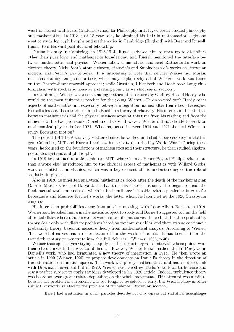
Wiener noted that Daniell had established a method to go from T0 to T1 but left open howto build I and T0 in the first place. Wiener proposed in this article to build these two objectsand to apply them to the case of functionals. For this, he used a simple notion of step functionsfor T0. We present here his construction step by step.

Let K be a set, we call In a division of the set K depending on a parameter n, a divisionof K being defined as a finite set of subsets, also called intervals, which cover K at least once.The intervals of the division In are denoted i1(In), ..., im(In). We no longer use the I notationfor the Daniell integral, so there is no confusion with the divisions. We can also assign a weightwIn (denoted wn if there is no ambiguity) to each interval of a division In, so that the intervalij(In) has the weight wn [ij(In)]. The division In is then said to be weighted by w. Finally, asequence {In}n∈N of divisions weighted by w is called a partition PK of the set K if it satisfiesthe following properties

(i) Each interval of In+1 is included in an interval of In and only one,(ii) The weight wn [ij(In)] of an interval ij(In) is the sum of the weights wn+1 [il(In+1)]

of the intervals il(In+1) included in ij(In).

There is a third condition that does not contribute anything to understanding, which we do notgive here for the sake of synthesis.

With these definitions, Wiener could then define his step functions. A function f defined onK is called a step function on PK if there is a division In belonging to the partition PK suchthat f is constant on each interval ij(In). Then Wiener defined the average APK (f) of a stepfunction f on PK intuitively as

APK (f) =

∑mj=1wn [ij(In)] f(xj)∑m

j=1wn [ij(In)], (4.4)

where xj ∈ ij(In).

Wiener then showed that his step functions satisfied the conditions of the set T0, given ineq. (4.1) by Daniell; and that his definition of the mean (eq. (4.4)) satisfied the axioms of theI operator, given in eq. (4.2). Using Daniell’s theorem, Wiener proved that all bounded anduniformly continuous functions on PK are summable in the sense of eq. (4.4). He thus had aconstruction of the mean of a function defined on any set K, potentially of infinite dimension.

To conclude his article, Wiener took some examples. By defining the In divisions in a simpleway and taking a segment for K, his definition of the average gave back Lebesgue’s one. Moreinterestingly, when he took for K the set of continuous functions defined on the interval [0, 1]

20

and null in 0, which we note C0[0, 1] from now on, which are in addition bounded and Lips-chitzian (then the functions defined on K were functionals by definition), then the applicationof the theorem gave that all continuous and bounded functionals were summable in the sense ofWiener.

In the following articles, Wiener gave more explicit definitions for the mean of a functional andapplied his axiomatic theory to the study of Brownian motion. The next article (Wiener, 1921a)was the first to explicitly deal with Brownian motion and was fundamental in the constructionof Wiener’s idealized Brownian motion, as we shall analyze now.

Wiener acknowledged Rene Gateaux’s work on the theory of functional average but claimedhis own version was more adapted to the case of Brownian movement than that of Gateaux.He began his article with a reference to Einstein’s work, and recalled this result: if a particleis free to move on the x axis and is subjected to Brownian motion, and if we assume that theprobability that it moves a certain value over a certain time interval is independent of

(i) its starting point,(ii) its starting absolute time,(iii) its direction,

then Einstein showed that the probability that after a time t the particle reached the positionx, written f(t) by Wiener, between x1 and x2, was under certain assumptions

P (x1 ≤ f(t) ≤ x2) =1√πt

∫ x2

x1

exp

(−x

2

t

)dx , (4.5)

where Wiener voluntarily omitted to note the physical parameter 4D, present in eq. (3.6), bysetting it equal to 1. The assumptions in question were not explained by Wiener but it is clearthat the one of the existence of a time scale τ on which the displacements are independentof previous displacements, was essential to the establishment of the Gaussian probability forEinstein. Wiener did not deal with the question of this time scale and used eq. (4.5) for all times,which made his object a simplified model of Brownian motion. In fact, he freed himself from thephysical difficulties that appeared when the mean free path was approached, and constructed amathematical model that made it possible to study Brownian motion by extending the range ofvalidity of the Gaussian distribution. It is this model that he continued to use in his subsequentarticles and which he described lucidly as follows

In the physical Brownian motion, it is of course true that the particle is not subject to anabsolutely perpetual influence resulting from the collision of the molecules but that there areshort intervals of time between one collision and the next. These, however, are far too short tobe observed by any ordinary methods. It therefore becomes natural to idealize the Brownianmotion as if the molecules were infinitesimal in size and the collisions continuously described.It was this idealized Brownian motion that I studied, and which I found to be an excellentsurrogate for the cruder properties of the true Brownian motion. (Wiener, 1956, p.39)

Let us go back to the article of 1921. To meet the conditions of his previous article, Wienerrestricted the parameter t ∈ [0, 1]. Thus the functions f(t), describing Brownian trajectories fellwithin the framework of the second example given in the previous article, and he could computethe average of the continuous and bounded functions defined on this set K of functions f(t).Wiener gave in this article a more explicit formula for the average of these functionals.Let us recall that functionals are defined as functions of functions, i.e. functions which do notdepend on a finite number of variables but of an entire function, which can be seen as an infinityof variables (i.e. f ≡ {f(t)}t∈[0,1]). Physically, these functionals of trajectories can be anyquantity that depends on the complete trajectory, such as the maximum value of the function,which represents the maximum distance the particle has moved away from its origin; or thelength of the trajectory.

21

Wiener started with a simple case where the functional F [f ], which we note with bracketsto differentiate it from a simple function, depended on f only for a finite number of valuesf(t1), ..., f(tn) in polynomial form: F [f ] = f(t1)m1 ...f(tn)mn . In this case F was rigorously afunction and not a functional, and the average of F was conventionally defined as the averageof a function

A(F ) =1√

πnt1(t2−t1)...(tn−tn−1)

+∞∫−∞

dx1...

+∞∫−∞

dxn xm11 ...xmnn exp

[−

n∑k=1

(xk−xk−1)2

tk−tk−1

].

(4.6)These integrals are analytically computable. Let us turn now to the most general case of truefunctionals. Wiener defined a general functional F [f ] by the expression

F [f ] = a0 +

∫ 1

0f(t)dψ1(t) + ...+

∫ 1

0...

∫ 1

0f(t1)...f(tn)dψn(t1, ..., tn) + ... . (4.7)

It was natural to require from the average operation to be stable by permutation with the sumof a series, by permutation with an integral, and by multiplication by a constant, which ledWiener to define the mean on this functional class as

A{F} = a0 +

∫ 1

0A(f(t))dψ1(t) + ...+

∫ 1

0...

∫ 1

0A(f(t1)...f(tn))dψn(t1, ..., tn) + ... , (4.8)

where we take care to note A{·} the average of a functional, defined by this formula, and A(·)the classical average of a function. The right-hand side is computable using eq. (4.6) for theterms A(f(t1)...f(tn)). As soon as this series converges, we have a definition for the mean of afunctional and a method relying on means of functions to compute it.

From here one can read Wiener’s work following two paths: the article (Wiener, 1922)19 fol-lowed the logic of the two articles that we just presented to refine the theory of the calculation offunctional average, and (Wiener, 1921b) deviated from this problem to deal on a concrete casecoming from Brownian movement. We choose to break the chronological order here to presentthe article (Wiener, 1922) first, because of its thematic filiation with the previous articles. Thearticle (Wiener, 1921b) deserves a sub-section (section 4.2.3) for itself because it was the onlyarticle closely related to the physicists’ Brownian movement and to experiments, and moreoverit has hardly been discussed in the literature.

The purpose of the 1922 article was to specify the partition PK used in the case of Brownianmotion, which had not been done in the article (Wiener, 1921a), and to use this partition toexpress the average of a functional having for argument a function representing the trajectoryof a Brownian particle.

Wiener chose once again the set K = C0[0, 1] and remarked that the distribution given byeq. (4.5) made it possible to assign weights to certain groups of trajectories which all passedthrough the same intervals at certain given times. Indeed, he set n time values between 0 and1: 0 ≤ t1 ≤ ... ≤ tn ≤ 1 and chose values xi1 and xi2 defining [xi1, xi2] windows through which

19The date of this article is uncertain, because its heading specified ‘Received February 27th, 1922.—Read March9th, 1922.’ and Wiener cited it in his 1930 article (Wiener, 1930) with the date 1922. However, this articleis mentioned with the date 1924 in the literature, as for example in Masani, 1990. Furthermore, in thisprecise article Wiener cited his 1923 article Differential Space, whereas in Differential Space he mentioned a‘forthcoming paper in Proc. Lond. Math. Soc.’ which is the 1922/24 article in question. It is then likely thatboth articles were written almost at the same time, during the year 1922, but were published in two differentjournals one year apart.

22

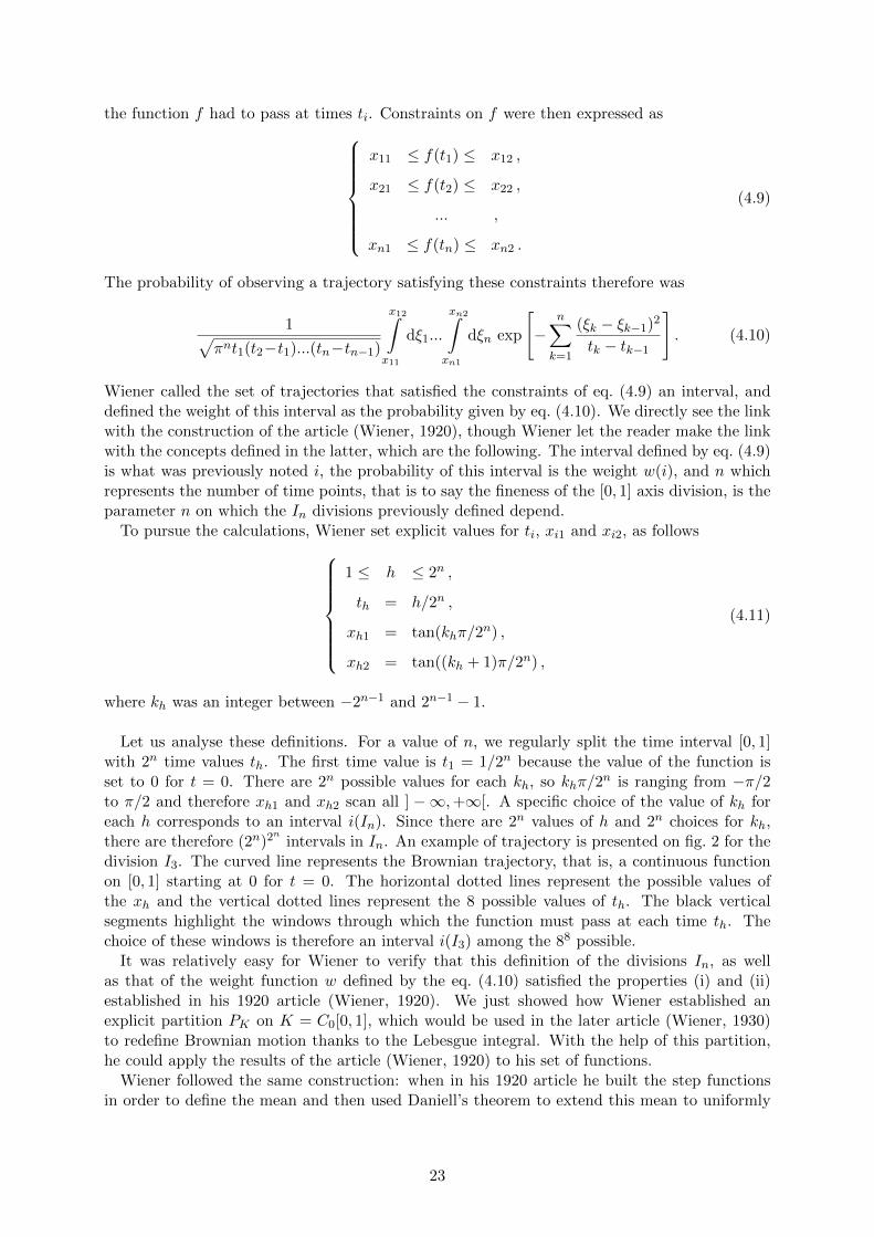
the function f had to pass at times ti. Constraints on f were then expressed as

x11 ≤ f(t1) ≤ x12 ,

x21 ≤ f(t2) ≤ x22 ,

... ,

xn1 ≤ f(tn) ≤ xn2 .

(4.9)

The probability of observing a trajectory satisfying these constraints therefore was

1√πnt1(t2−t1)...(tn−tn−1)

x12∫x11

dξ1...

xn2∫xn1

dξn exp

[−

n∑k=1

(ξk − ξk−1)2

tk − tk−1

]. (4.10)

Wiener called the set of trajectories that satisfied the constraints of eq. (4.9) an interval, anddefined the weight of this interval as the probability given by eq. (4.10). We directly see the linkwith the construction of the article (Wiener, 1920), though Wiener let the reader make the linkwith the concepts defined in the latter, which are the following. The interval defined by eq. (4.9)is what was previously noted i, the probability of this interval is the weight w(i), and n whichrepresents the number of time points, that is to say the fineness of the [0, 1] axis division, is theparameter n on which the In divisions previously defined depend.

To pursue the calculations, Wiener set explicit values for ti, xi1 and xi2, as follows

1 ≤ h ≤ 2n ,

th = h/2n ,

xh1 = tan(khπ/2n) ,

xh2 = tan((kh + 1)π/2n) ,

(4.11)

where kh was an integer between −2n−1 and 2n−1 − 1.

Let us analyse these definitions. For a value of n, we regularly split the time interval [0, 1]with 2n time values th. The first time value is t1 = 1/2n because the value of the function isset to 0 for t = 0. There are 2n possible values for each kh, so khπ/2

n is ranging from −π/2to π/2 and therefore xh1 and xh2 scan all ] −∞,+∞[. A specific choice of the value of kh foreach h corresponds to an interval i(In). Since there are 2n values of h and 2n choices for kh,there are therefore (2n)2n intervals in In. An example of trajectory is presented on fig. 2 for thedivision I3. The curved line represents the Brownian trajectory, that is, a continuous functionon [0, 1] starting at 0 for t = 0. The horizontal dotted lines represent the possible values ofthe xh and the vertical dotted lines represent the 8 possible values of th. The black verticalsegments highlight the windows through which the function must pass at each time th. Thechoice of these windows is therefore an interval i(I3) among the 88 possible.

It was relatively easy for Wiener to verify that this definition of the divisions In, as wellas that of the weight function w defined by the eq. (4.10) satisfied the properties (i) and (ii)established in his 1920 article (Wiener, 1920). We just showed how Wiener established anexplicit partition PK on K = C0[0, 1], which would be used in the later article (Wiener, 1930)to redefine Brownian motion thanks to the Lebesgue integral. With the help of this partition,he could apply the results of the article (Wiener, 1920) to his set of functions.

Wiener followed the same construction: when in his 1920 article he built the step functionsin order to define the mean and then used Daniell’s theorem to extend this mean to uniformly

23

458 N

OR

BE

RT

WIE

NE

R

of tx and t2 between 0 and 1, inclusive,

[March 9,

where h is a given positive integer.

These functions are m

anifestly what

Ascoli* calls equally continuous, and are bounded as a set.

They therefore

form

what

Frechett

calls a com

pact set,

and there

is no difficulty

in

* Ascoli, " L

e curve limiti di una varieta data di curve ", L

ined, Vol. 18, pp. 521-58G

.t

M. F

rechefc,." Sur quelques points

du calcul

fonctionnel", R

end. Civ. M

at I'aL

,V

ol. 22, pp. G, 37.

Figure 2: Example of a path going through the windows of a particular interval i(I3). The imagehas been rotated by 90 ° compared to the one in the original article.

continuous and bounded functions understood as limits of step functions series; in this articlehe defined the step functional in the same way and then extended the average operation tofunctionals that are limits of step functionals series. He defined a step functional as takingconstant values on each interval i(In) of a certain division In. The average of a step functionalwas then naturally given by

A{F} =∑k

F [f ]w[ik(In)] , (4.12)

where f ∈ ik(In).Wiener was finally able to apply Daniell’s theorem and he deduced that all bounded and

continuous functionals, defined on Brownian trajectories, were summable. Moreover the averagevalue was given by the formula

A{F} = limmax(ti+1−ti)→0

π−n/2n∏k=1

(tk − tk−1)−1/2

+∞∫−∞

dx1...

+∞∫−∞

dxn

F [{ψ(t1, ..., tn)(x1, ..., xn)}(t)] exp

[−

n∑k=1

(xk − xk−1)2

tk − tk−1

]. (4.13)

where Wiener set F [{ψ(t1, ..., tn)(x1, ..., xn)}(t)] = Ft1,...,tn [f ] the step functional only dependingof f(t1), ..., f(tn).

24

4.2.3. Developments on Einstein’s formula - 1921

The article on which we focus now was quite particular in Wiener’s bibliography. As we al-ready noted, it was hardly ever discussed in the literature, maybe because it was the only onethat did not offer novelties from a mathematical point of view, but it is even more interesting tonote that Wiener chose a different position compared to his other articles by assuming that thevelocities of Brownian particles existed. This article was thus a parenthesis in Wiener’s journey,inside which he used a model close to that of Ornstein-Uhlenbeck, which is discussed in section 5 .

For the first time, Wiener gave a review of the physicists’ Brownian movement, which wasquite detailed, quoting Einstein and Perrin, explaining the physical origin of the phenomenon interms of collisions and noting the difference between theoretical and measured velocities due tothe ‘extreme sinuosity of the trajectories’. According to him, Einstein made two assumptions:

(i) the validity of Stokes’ law at the scale of Brownian particles,(ii) the independence of increments over time intervals τ .

His objective was to use the results obtained in his previous article to demonstrate that Einstein’sformula on the mean square of displacements (eq. (3.8)) did not in fact require the secondhypothesis to be true.

Wiener began by defining a function f(ct) as the total momentum of the Brownian particleacquired by the collisions with the other molecules only, up to the time t. This was a differentdefinition from the previous article where f(t) was the position of the particle at time t. Theconstant c which depends on the physical parameters must now be noted explicitly because ithas an impact on numerical calculations. Wiener could have redefined the normal distribution ofeq. (4.5) to include c but he chose to use c as an argument of the f function directly, to preservethe form of f(t) and thus make the results obtained in the previous article usable. Accordingto him the distribution of f was then given by

P (a ≤ f(ct) ≤ b) =1√πct

∫ b

aexp

(−x

2

ct

)dx . (4.14)

One must note that a, b and x have the dimension of a momentum, that is to say kg m s−1,which makes c a quantity expressed in kg2m3/s3.

Wiener’s starting point was an equation similar to Newton’s second law:

m [v(t+ dt)− v(t)] = f(ct+ cdt)− f(ct)− 6πµav(t+ δ · dt)dt (0 ≤ δ ≤ 1) . (4.15)

In this equation the role of collisions was taken into account by f(ct+cdt)−f(ct), which appearedas an analogue of Langevin’s force X in eq. (3.14). The last term accounted for the viscosity andδ could vary between 0 and 1, probably to allow the choice of any point of the interval [t; t+ dt]for the value of the velocity. However this factor did not matter as it would disappear in thenext calculation step. Wiener did not make any assumptions about the function f , in particularhe did not suppose it to be differentiable, which explained this writing in infinitesimal form. Heintegrated this equation to obtain

m [v(t)− v0] = f(ct)− 6πµa

∫ t

0v(t′)dt′ , (4.16)

where v0 was the initial velocity of the particle. He solved this equation and wrote

mv(t) = mv0e−βt + f(ct)− βe−βt

∫ t

0f(ct′)eβt

′dt′ , (4.17)

25

where we set, in order to simplify the writings,

β =6πµa

m, (4.18)

which is the inverse of the characteristic time θ defined by Langevin in eq. (3.18).Since he obtained the velocity, Wiener had to integrate to get the position, then square the

expression and take the mean to shape the result in a similar way to that of Einstein. The firststep reads

x(t) =

∫ t

0v(t′)dt′ =

v0

β

(1− e−βt

)+e−βt

mc

∫ T

0eβT

′/cf(T ′)dT ′ , (4.19)

where he made the change of variable T = ct in the integral. Since x(t) is a functional off , the average of x2(t) in the sense of Wiener is therefore written A

{x2(t)

}(analogue of λ2

x inEinstein’s notation) and it is an average over the different realizations of the function f weightedby their probabilities according to eq. (4.14).

A{x2(t)

}= A

{v2

0

β2

(1− e−βt

)2+e−2βt

m2c2

∫ T

0

∫ T

0eβ(T1+T2)/cf(T1)f(T2)dT1dT2

+2v0e

−βt

mβc

(1− e−βt

)∫ T

0eβT

′/cf(T ′)dT ′}. (4.20)

It was at this moment that Wiener used eqs. (4.6) and (4.8) from his previous article, whichallowed him to suppress the term in {f(T )}, and to explicitly compute the term in {f(T1)f(T2)}as

A

{∫ T

0

∫ T

0f(T1)f(T2)H(T1, T2)dT1dT2

}=

∫ T

0

∫ T2

0T1H(T1, T2)dT1dT2 , (4.21)

in the case where H(T1, T2) = H(T2, T1), which is our case. After replacement, the formulareads

A{x2(t)

}=v2

0

β2

(1− e−βt

)2+e−2βt

m2c2

∫ T

0

[∫ T2

0T1e

β(T1+T2)/cdT1

]dT2 . (4.22)

Wiener then computed the double integral of the right-hand side and wrote the final result asfollows

A{x2(t)

}=v2

0

β2

(1− e−βt

)2+

c

4m2β3

[2βt− 3 + 4e−βt − e−2βt

]. (4.23)

It appears that the linearity between the average of the squares of displacements and the timecomes from the term ct/(2m2β2) in the right-hand side, thus if one wishes to obtain a resultsimilar to Einstein’s one, one must make sure that this term is dominant. Hence, Wiener choseto express the absolute value of the difference between A

{x2(t)

}and this particular term∣∣∣∣∣A

{x2(t)

}t

− c

2m2β2

∣∣∣∣∣ =1

t

∣∣∣∣ v20

β2

(1− e−βt

)2+

c

4m2β3(3− e−βt)(1− e−βt)

∣∣∣∣ . (4.24)

From this equality, Wiener deduced without justification the following inequality∣∣∣∣∣A{x2(t)

}t

− c

2m2β2

∣∣∣∣∣ ≤ v20

β2+

3c

4m2β3. (4.25)

It appears that he replaced the exponentials by 0 to obtain an upper bound of the right handside, giving that all the terms are positive, but that he forgot to put back the term 1/t, thusgiving a result that was not homogeneous from a physical point of view. For the sake of clarity,we from now on write this missing factor explicitly in the equations.

26

The last step of Wiener’s reasoning consisted in defining the relative deviation as follows∣∣A{x2(t)}/t− c/(2m2β2)

∣∣c/(2m2β2)

≤ 1

t

[2m2v2

0

c+

3

2β

]. (4.26)

In order to estimate the right-hand side, Wiener finally referred to Perrin’s values on gamboge,without precisely mentioning which ones, and obtained the value 10−8 for the absolute relativeerror.

Let us investigate how Wiener obtained the value 10−8. First, we replace the mathematicalnotations by their physical counterparts. In Wiener’s calculation, the nominal value of λ2

x wasc/2m2β2 and in Einstein’s theory it was kBT/3πµa, hence by equalizing the two quantities andusing the definition of β given in eq. (4.18) we obtain

c = 24πµakBT . (4.27)

After replacement, eq. (4.26) reads

|λx/t− kBT/(3πµa)|kBT/(3πµa)

≤ 1

t

[m2v2

0

12πµakBT+

m

4πµa

]. (4.28)

We can suppose the equipartition of energy for the initial velocity, as done by Ornstein insection 5, and thus replace mv2

0 by kBT (in the one-dimensional case) to obtain

|λx/t− kBT/(3πµa)|kBT/(3πµa)

≤ 1

t

m

3πµa. (4.29)

Wiener did not mention the particular set of Perrin’s values on gamboge he used but we lookedat the ones Perrin gave in Les Atomes. On page 182 appears a table of results for severalexperiments with gamboge, let us choose the line 6 for which the experiment have workedthe best, since it was the one that gave the best value for Avogadro’s number. The values areµ = 1.25 kg m−1 s−1, a = 0.385 µm and m = 0.29× 10−12 kg. Replacing these values in eq. (4.29)ans choosing20 t = 1 s, we get 6.4× 10−8, which is in agreement with the order of magnitudecalculated by Wiener.

We can also note that the right-hand side of eq. (4.29) is indeed 2θ/t where θ is the character-istic time scale defined by Langevin (eq. (3.18)), whose value is 10−8 s according to him. Onceagain the result is compatible with Wiener’s one.

Let us analyze how Wiener’s mistake impacted the assumption he was trying to prove. Hewanted to prove that the hypothesis made by Einstein on the independence of the displacementson disjoint successive time intervals was in fact not necessary, by showing that the result heobtained without making this assumption was so close to Einstein’s result that the differencecould not be observed experimentally. Therefore, the ‘slightly different value of λx/t for smallvalues of the time than for larger values’ observed by experimenters was, according to Wiener,to be traced to the hypothesis (i): a violation of Stokes’ law at this scale. However, time t didnot appear in the final formula that bounded the absolute relative mistake, so maybe Wienerthought that his value 10−8 held for any time t, and thus even for very small values of t, henceprecisely in the case where discrepancies had been observed. In reality, the upper bound on therelative error is inversely proportional to time t, so for very small values of t the upper limitbecomes large, making Wiener’s conclusion possibly false. This bound reads 2/βt, so if the

20Indeed, since this factor t did not appear in Wiener’s equation at this stage of the calculation, it seemed logicalto us to compute this quantity numerically with the value t = 1 s. Of course, in reality the error increases ast decreases so the value 10−8 is not a physical limit.

27

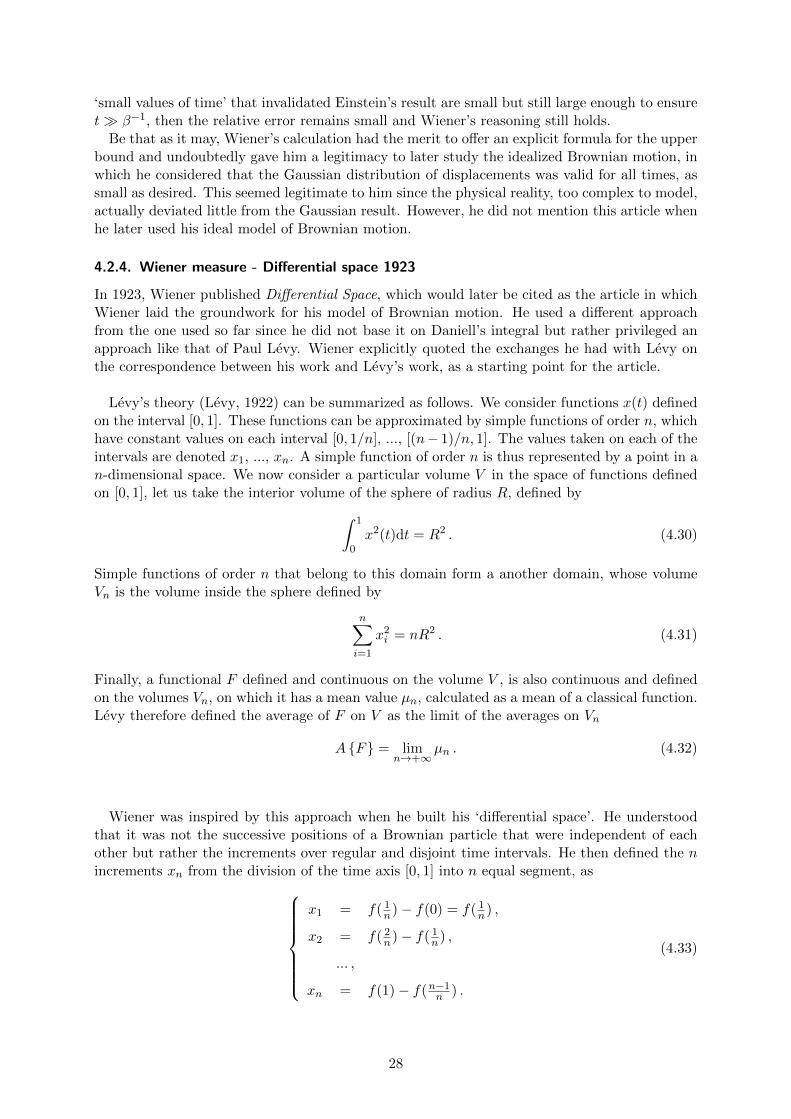
‘small values of time’ that invalidated Einstein’s result are small but still large enough to ensuret� β−1, then the relative error remains small and Wiener’s reasoning still holds.

Be that as it may, Wiener’s calculation had the merit to offer an explicit formula for the upperbound and undoubtedly gave him a legitimacy to later study the idealized Brownian motion, inwhich he considered that the Gaussian distribution of displacements was valid for all times, assmall as desired. This seemed legitimate to him since the physical reality, too complex to model,actually deviated little from the Gaussian result. However, he did not mention this article whenhe later used his ideal model of Brownian motion.

4.2.4. Wiener measure - Differential space 1923

In 1923, Wiener published Differential Space, which would later be cited as the article in whichWiener laid the groundwork for his model of Brownian motion. He used a different approachfrom the one used so far since he did not base it on Daniell’s integral but rather privileged anapproach like that of Paul Levy. Wiener explicitly quoted the exchanges he had with Levy onthe correspondence between his work and Levy’s work, as a starting point for the article.

Levy’s theory (Levy, 1922) can be summarized as follows. We consider functions x(t) definedon the interval [0, 1]. These functions can be approximated by simple functions of order n, whichhave constant values on each interval [0, 1/n], ..., [(n− 1)/n, 1]. The values taken on each of theintervals are denoted x1, ..., xn. A simple function of order n is thus represented by a point in an-dimensional space. We now consider a particular volume V in the space of functions definedon [0, 1], let us take the interior volume of the sphere of radius R, defined by∫ 1

0x2(t)dt = R2 . (4.30)

Simple functions of order n that belong to this domain form a another domain, whose volumeVn is the volume inside the sphere defined by

n∑i=1

x2i = nR2 . (4.31)

Finally, a functional F defined and continuous on the volume V , is also continuous and definedon the volumes Vn, on which it has a mean value µn, calculated as a mean of a classical function.Levy therefore defined the average of F on V as the limit of the averages on Vn

A {F} = limn→+∞

µn . (4.32)

Wiener was inspired by this approach when he built his ‘differential space’. He understoodthat it was not the successive positions of a Brownian particle that were independent of eachother but rather the increments over regular and disjoint time intervals. He then defined the nincrements xn from the division of the time axis [0, 1] into n equal segment, as

x1 = f( 1n)− f(0) = f( 1

n) ,

x2 = f( 2n)− f( 1

n) ,

... ,

xn = f(1)− f(n−1n ) .

(4.33)

28

These n quantities were independent and had the same statistical weight in the sense that theycontributed to the displacement of the particle over equal periods of time, so it seemed naturalfor Wiener to use Levy’s formulation and to consider the sphere defined by

n∑i=1

x2i = R2

n . (4.34)

To test the relevance of this definition, Wiener raised the question of measuring the inner regionof the sphere where the position f(a) was between y1 and y2, i.e. µ(y1 ≤ f(a) =

∑nak=1 xk ≤ y2),

where the notation µ is used for the measure. In the case where Rn = R was a constant, Wienerproved that this measure took the value

µ(y1 ≤ f(a) ≤ y2) =1√

2πaR2

∫ y2

y1

exp(− u

2aR2

)du . (4.35)

This measure was of the same form as the probability given by eq. (4.5), which showed that theLevy sphere seemed to be an appropriate tool to study Brownian trajectories. Wiener then calledthe set of functions f(t), along with the measure µ defined as the limit of the measures given ineq. (4.35), the differential space, to reflect the fact that it is the differences that are independent.

Wiener returned to his major concern: the definition of the average of a functional. He beganonce again with the simple case of a functional that depended on a function only by a finitenumber of its values. He took n points 0 ≤ t1 ...tn ≤ 1 and divided the segment [0, 1] into ν parts,all of size 1/ν. ν must be large enough for only one ti value to be included in each interval. Hethen defined the step function fν(t) which took the values of f for each value of ti: ∀i, fν(ti) =f(ti). He could then define the differences on the function fν : xk = fν(k/ν) − fν((k − 1)/ν).Finally, the values f(t1), ... f(tn) on which depended the functional F could be expressed interms of these differences: f(ti) = fν(Ti/ν) = x1 + x2 + ...+ xTi where he defined Ti = νti if νtiwas an integer, or the first higher integer otherwise.

He was thus in the position of applying the formalism he established before, placing himselfin the volume defined by the interior of the sphere

∑ni=1 x

2i = R2. The average of the functional

within this sphere was properly defined, and if it reached a value when taking the limit, he couldspeak of the average of this functional on the differential space. The average of F in the spheredefined above was

A{F} = (2πR2)−n/2n∏k=1

(tk − tk−1)−1/2

×+∞∫−∞

dy1...

+∞∫−∞

dyn F [y1, ..., yn] exp

[−

n∑k=1

y2k

2R2(tk − tk−1)

]. (4.36)

Moreover, Wiener defined the measure of a domain of this sphere by choosing for the functionalF the value 1 if the argument function laid in the considered domain and 0 otherwise. To givean example, he defined the following domain

y11 ≤ y1 ≤ y12 ,

y21 ≤ y2 ≤ y22 ,

... ,

yn1 ≤ yn ≤ yn2 ,

(4.37)

29

which was none other than the domain previously defined in eq. (4.9). Wiener measure of thedomain defined by eq. (4.37) was

(2πR2)−n/2n∏k=1

(tk − tk−1)−1/2

y12∫y11

dy1...

yn2∫yn1

dyn exp

[−

n∑k=1

y2k

2R2(tk − tk−1)

]. (4.38)

This long article was full of other rich ideas but we chose to focus on the one that was a firststep towards the non-differentiability of Brownian trajectories.

Wiener reversed the previous perspective, in which he was interested in the distribution off(a) =

∑nak=1 xk with the constraint

∑ni=1 x

2i = R2. Inversely, he raised the question of the

distribution of∑n

i=1 x2i =

∑ni=1 [f(i/n)− f((i− 1)/n)]2 assuming that the increments f(t2) −

f(t1) were independent and had a Gaussian distribution. He demonstrated that the quantity∑ni=1 x

2i only deviated from D with a small probability, where D was the physical diffusion

coefficient.

∀ε > 0, ∀δ > 0, P

(∣∣∣∣∣ limn→+∞

n∑1

[f

(k

n

)− f

(k − 1

n

)]2

−D

∣∣∣∣∣ > δ

)< ε , (4.39)

Next, he considered the particular case of a continuous functions f , of limited total variation.

n∑k=1

[f

(k

n

)− f

(k − 1

n

)]2

≤ maxk

∣∣∣∣f (kn)− f

(k − 1

n

)∣∣∣∣ n∑k=1

∣∣∣∣f (kn)− f

(k − 1

n

)∣∣∣∣≤ T (f) ·max

k

∣∣∣∣f (kn)− f

(k − 1

n

)∣∣∣∣ , (4.40)

where T (f) was the total variation of the function f over [0, 1]. We recall that the total vari-ation of a function f is a possible measure of its arc length and can be defined as T (f) =supP

∑nk=1 |f (k/n)− f ((k − 1)/n)| where P denotes the set of partitions (in the modern sense,

not that of PK) of [0, 1].When making n tend to infinity in eq. (4.40), the upper bound in the right-hand side went to 0.

Since Wiener showed that in the case of Brownian trajectories the quantity∑n

i=1 [f(i/n)− f((i− 1)/n)]2

did not tend to 0 but was close to D, he therefore deduced that it was infinitely unlikely forBrownian trajectories to be of limited total variation and therefore infinitely unlikely that theyhave a bounded derivative.

Wiener called the coefficient limn→∞∑n

i=1 [f(i/n)− f((i− 1)/n)]2 ‘a kind of coefficient ofnon-differentiability of the function f ’21 because it measured a degree of non-differentiabilityequal to its deviation from 0.

4.2.5. Lebesgue measure and stochastic processes - 1930

The next advances in Brownian motion modelling came later, in the 1930s, with a thesis onharmonic analysis published in 1930 by Wiener (Wiener, 1930) and with the collaboration withmathematicians Paley and Zygmund in 1932-1933, which culminated to a fundamental articlein 1933 (Paley et al., 1933). In his 1930 article, Wiener gave a new formulation of Brownianmotion, in terms of Lebesgue measure, and it was this formulation that allowed Brownian mo-tion to be considered as a stochastic process in the 1933 article. This led to the proof of thenon-differentiability of Brownian trajectories, which ends our history of mathematical Brownian

21It should be noted that in the article it was the quantity limn→∞∑ni=1

[f(i/n)− f((i− 1)/n)2

]that Wiener

called the coefficient of non-differentiability but it was a printing error, as there were several in the article.

30

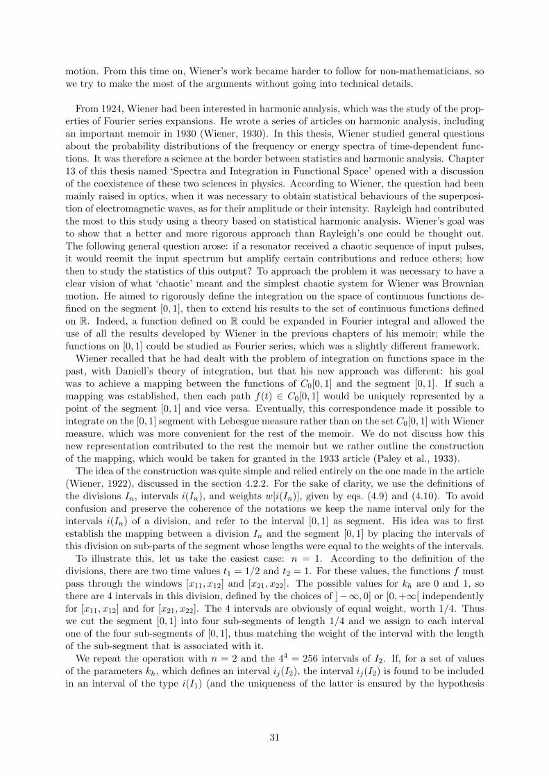
motion. From this time on, Wiener’s work became harder to follow for non-mathematicians, sowe try to make the most of the arguments without going into technical details.

From 1924, Wiener had been interested in harmonic analysis, which was the study of the prop-erties of Fourier series expansions. He wrote a series of articles on harmonic analysis, includingan important memoir in 1930 (Wiener, 1930). In this thesis, Wiener studied general questionsabout the probability distributions of the frequency or energy spectra of time-dependent func-tions. It was therefore a science at the border between statistics and harmonic analysis. Chapter13 of this thesis named ‘Spectra and Integration in Functional Space’ opened with a discussionof the coexistence of these two sciences in physics. According to Wiener, the question had beenmainly raised in optics, when it was necessary to obtain statistical behaviours of the superposi-tion of electromagnetic waves, as for their amplitude or their intensity. Rayleigh had contributedthe most to this study using a theory based on statistical harmonic analysis. Wiener’s goal wasto show that a better and more rigorous approach than Rayleigh’s one could be thought out.The following general question arose: if a resonator received a chaotic sequence of input pulses,it would reemit the input spectrum but amplify certain contributions and reduce others; howthen to study the statistics of this output? To approach the problem it was necessary to have aclear vision of what ‘chaotic’ meant and the simplest chaotic system for Wiener was Brownianmotion. He aimed to rigorously define the integration on the space of continuous functions de-fined on the segment [0, 1], then to extend his results to the set of continuous functions definedon R. Indeed, a function defined on R could be expanded in Fourier integral and allowed theuse of all the results developed by Wiener in the previous chapters of his memoir; while thefunctions on [0, 1] could be studied as Fourier series, which was a slightly different framework.

Wiener recalled that he had dealt with the problem of integration on functions space in thepast, with Daniell’s theory of integration, but that his new approach was different: his goalwas to achieve a mapping between the functions of C0[0, 1] and the segment [0, 1]. If such amapping was established, then each path f(t) ∈ C0[0, 1] would be uniquely represented by apoint of the segment [0, 1] and vice versa. Eventually, this correspondence made it possible tointegrate on the [0, 1] segment with Lebesgue measure rather than on the set C0[0, 1] with Wienermeasure, which was more convenient for the rest of the memoir. We do not discuss how thisnew representation contributed to the rest the memoir but we rather outline the constructionof the mapping, which would be taken for granted in the 1933 article (Paley et al., 1933).

The idea of the construction was quite simple and relied entirely on the one made in the article(Wiener, 1922), discussed in the section 4.2.2. For the sake of clarity, we use the definitions ofthe divisions In, intervals i(In), and weights w[i(In)], given by eqs. (4.9) and (4.10). To avoidconfusion and preserve the coherence of the notations we keep the name interval only for theintervals i(In) of a division, and refer to the interval [0, 1] as segment. His idea was to firstestablish the mapping between a division In and the segment [0, 1] by placing the intervals ofthis division on sub-parts of the segment whose lengths were equal to the weights of the intervals.

To illustrate this, let us take the easiest case: n = 1. According to the definition of thedivisions, there are two time values t1 = 1/2 and t2 = 1. For these values, the functions f mustpass through the windows [x11, x12] and [x21, x22]. The possible values for kh are 0 and 1, sothere are 4 intervals in this division, defined by the choices of ]−∞, 0] or [0,+∞[ independentlyfor [x11, x12] and for [x21, x22]. The 4 intervals are obviously of equal weight, worth 1/4. Thuswe cut the segment [0, 1] into four sub-segments of length 1/4 and we assign to each intervalone of the four sub-segments of [0, 1], thus matching the weight of the interval with the lengthof the sub-segment that is associated with it.

We repeat the operation with n = 2 and the 44 = 256 intervals of I2. If, for a set of valuesof the parameters kh, which defines an interval ij(I2), the interval ij(I2) is found to be includedin an interval of the type i(I1) (and the uniqueness of the latter is ensured by the hypothesis

31

(i) of the partitions, discussed in section 4.2.2), then we place the sub-segment correspondingto ij(I2), the length of which is defined by the weight of this interval, inside the sub-segmentcorresponding to i(I1).

Wiener repeated the operation with n → +∞. The intervals of the successive divisions thusfitted in infinitely until reaching sub-segments of zero length. Thus each point of the segmentwas determined by an infinite sequence of intervals whose weights tend to 0, defining a uniquetrajectory of zero probability. Wiener therefore completed the construction of the mapping be-tween the points of the [0, 1] segment and the functions of C0[0, 1].

In 1933, Wiener, Paley and Zygmund published an article together, that aimed at establishinga correspondence between Wiener’s theory on the one hand, and Paley and Zygmund’s theory onthe other hand. Indeed, the two theories dealt with the introduction of randomness in analysisbut with different approaches, which could be unified. Paley and Zygmund’s work focused onthe study of random-coefficients series, initiated by Borel, and that of Wiener dealt with thestudy of random trajectories such as those of Brownian motion, whose study he reduced toa problem of Lebesgue integration, as we saw previously. The aim was therefore to establishsimilar theorems to those obtained by Paley and Zygmund for the random functions studied byWiener.

We present here two aspects of this paper: the formalism used to describe Wiener’s randomfunctions and the Theorem VII, which established the almost surely non-differentiability ofBrownian trajectories.

The authors proposed to represent

one of the components of the displacement of the moving particle in the Wiener theory byχ(α, t), where t is the time and α the parameter on which Lebesgue integration is performedfor the purpose of averaging over all functions and determining probabilities. Wiener’s χ(α, t)is then, as he shows, a continuous function of t for almost all values of α, defined for 0 ≤ α ≤ 1,0 ≤ t ≤ 1 and vanishing for t = 0.

This definition may seem surprising at first glance, but it was nevertheless the way to definethe stochastic processes later (for example in (Doob, 1966)) and it still is today. α is a numberbetween 0 and 1, which according to the mapping established by Wiener in the previous articlerepresents a function of C0[0, 1], which we also note α. We observe a change of perspective,rather than denoting α(t) a component of the trajectory of a Brownian particle, we use a χfunction with two variables, taking as argument both the time t and the trajectory α. Anenlightening interpretation of this quantity was given in (Doob, 1966).χ(α, t) must be understood as the value of the α trajectory at time t, i.e. χ(α, t) = α(t).

Then χ(α, ·), seen as a function of t, is a trajectory, or a realization, of the stochastic process.With this formalism, Joseph Leo Doob summarized the properties Wiener had established onBrownian motion as

(i) Its increments are Gaussian: χ(·, t) is a random variable on C0[0, 1], following thenormal law (χ(·, t2)− χ(·, t1)) ∼ N (0, σ2|t2 − t1|),

(ii) its increments on disjoint time intervals are independent: ∀ 0 ≤ t0 ≤ ... ≤ tn ≤ 1,random variables χ(·, t1)− χ(·, t0), ..., χ(·, tn)− χ(·, tn−1) are independent.

Let us go back to the 1933 article. The authors obtained, once more, the formula of theaverage of a functional when this one depended only on a finite number of values given at times

32

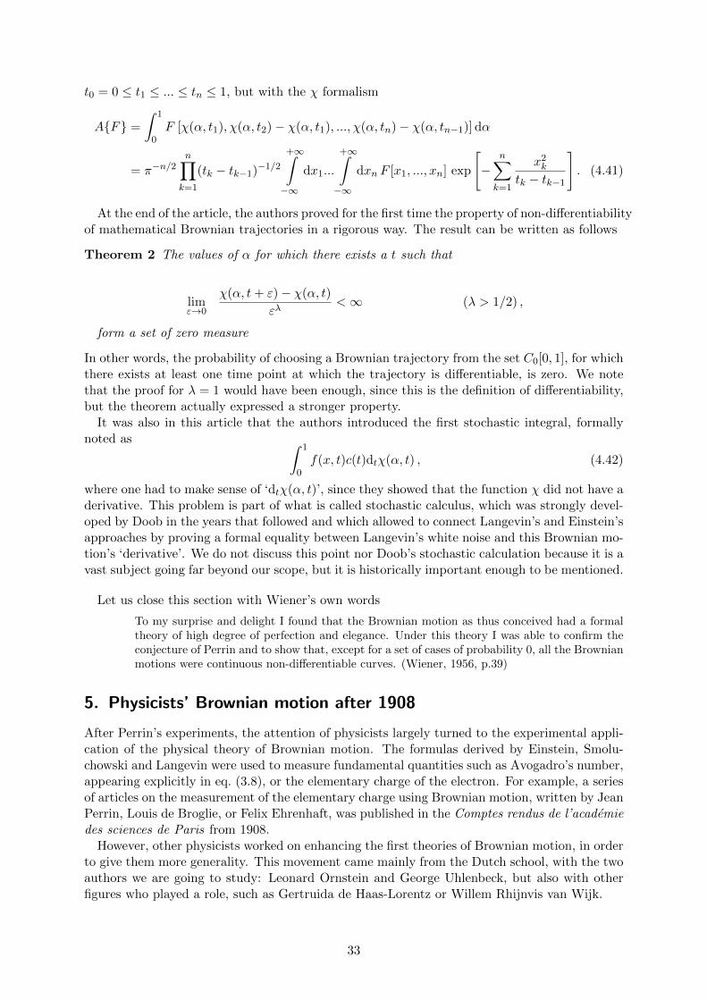
t0 = 0 ≤ t1 ≤ ... ≤ tn ≤ 1, but with the χ formalism

A{F} =

∫ 1

0F [χ(α, t1), χ(α, t2)− χ(α, t1), ..., χ(α, tn)− χ(α, tn−1)] dα

= π−n/2n∏k=1

(tk − tk−1)−1/2

+∞∫−∞

dx1...

+∞∫−∞

dxn F [x1, ..., xn] exp

[−

n∑k=1

x2k

tk − tk−1

]. (4.41)

At the end of the article, the authors proved for the first time the property of non-differentiabilityof mathematical Brownian trajectories in a rigorous way. The result can be written as follows

Theorem 2 The values of α for which there exists a t such that

limε→0

χ(α, t+ ε)− χ(α, t)

ελ<∞ (λ > 1/2) ,

form a set of zero measure

In other words, the probability of choosing a Brownian trajectory from the set C0[0, 1], for whichthere exists at least one time point at which the trajectory is differentiable, is zero. We notethat the proof for λ = 1 would have been enough, since this is the definition of differentiability,but the theorem actually expressed a stronger property.

It was also in this article that the authors introduced the first stochastic integral, formallynoted as ∫ 1

0f(x, t)c(t)dtχ(α, t) , (4.42)

where one had to make sense of ‘dtχ(α, t)’, since they showed that the function χ did not have aderivative. This problem is part of what is called stochastic calculus, which was strongly devel-oped by Doob in the years that followed and which allowed to connect Langevin’s and Einstein’sapproaches by proving a formal equality between Langevin’s white noise and this Brownian mo-tion’s ‘derivative’. We do not discuss this point nor Doob’s stochastic calculation because it is avast subject going far beyond our scope, but it is historically important enough to be mentioned.

Let us close this section with Wiener’s own words

To my surprise and delight I found that the Brownian motion as thus conceived had a formaltheory of high degree of perfection and elegance. Under this theory I was able to confirm theconjecture of Perrin and to show that, except for a set of cases of probability 0, all the Brownianmotions were continuous non-differentiable curves. (Wiener, 1956, p.39)

5. Physicists’ Brownian motion after 1908

After Perrin’s experiments, the attention of physicists largely turned to the experimental appli-cation of the physical theory of Brownian motion. The formulas derived by Einstein, Smolu-chowski and Langevin were used to measure fundamental quantities such as Avogadro’s number,appearing explicitly in eq. (3.8), or the elementary charge of the electron. For example, a seriesof articles on the measurement of the elementary charge using Brownian motion, written by JeanPerrin, Louis de Broglie, or Felix Ehrenhaft, was published in the Comptes rendus de l’academiedes sciences de Paris from 1908.

However, other physicists worked on enhancing the first theories of Brownian motion, in orderto give them more generality. This movement came mainly from the Dutch school, with the twoauthors we are going to study: Leonard Ornstein and George Uhlenbeck, but also with otherfigures who played a role, such as Gertruida de Haas-Lorentz or Willem Rhijnvis van Wijk.

33

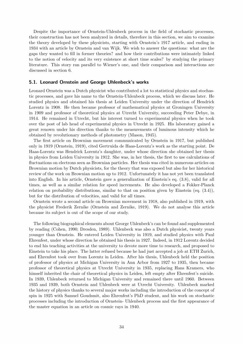
Despite the importance of Ornstein-Uhlenbeck process in the field of stochastic processes,their construction has not been analyzed in details, therefore in this section, we aim to examinethe theory developed by these physicists, starting with Ornstein’s 1917 article, and ending in1934 with an article by Ornstein and van Wijk. We wish to answer the questions: what are thegaps they wanted to fill in former theories? and how their contributions were intimately linkedto the notion of velocity and its very existence at short time scales? by studying the primaryliterature. This story ran parallel to Wiener’s one, and their comparison and interactions arediscussed in section 6.

5.1. Leonard Ornstein and George Uhlenbeck’s works

Leonard Ornstein was a Dutch physicist who contributed a lot to statistical physics and stochas-tic processes, and gave his name to the Ornstein-Uhlenbeck process, which we discuss later. Hestudied physics and obtained his thesis at Leiden University under the direction of HendrickLorentz in 1908. He then became professor of mathematical physics at Groningen Universityin 1909 and professor of theoretical physics at Utrecht University, succeeding Peter Debye, in1914. He remained in Utrecht, but his interest turned to experimental physics when he tookover the post of lab head of experimental physics in Utrecht in 1925. His laboratory gained agreat renown under his direction thanks to the measurements of luminous intensity which heobtained by revolutionary methods of photometry (Mason, 1945).

The first article on Brownian movement communicated by Ornstein in 1917, but publishedonly in 1919 (Ornstein, 1919), cited Gertruida de Haas-Lorentz’s work as the starting point. DeHaas-Lorentz was Hendrick Lorentz’s daughter, under whose direction she obtained her thesisin physics from Leiden University in 1912. She was, in her thesis, the first to use calculations offluctuations on electrons seen as Brownian particles. Her thesis was cited in numerous articles onBrownian motion by Dutch physicists, for the theory that was exposed but also for her historicalreview of the work on Brownian motion up to 1912. Unfortunately it has not yet been translatedinto English. In his article, Ornstein gave a generalization of Einstein’s eq. (3.8), valid for alltimes, as well as a similar relation for speed increments. He also developed a Fokker-Planckrelation on probability distributions, similar to that on position given by Einstein (eq. (3.4)),but for the distribution of velocities, and valid for all times.

Ornstein wrote a second article on Brownian movement in 1918, also published in 1919, withthe physicist Frederik Zernike (Ornstein and Zernike, 1919). We do not analyse this articlebecause its subject is out of the scope of our study.

The following biographical elements about George Uhlenbeck’s can be found and supplementedby reading (Cohen, 1990; Dresden, 1989). Uhlenbeck was also a Dutch physicist, twenty yearsyounger than Ornstein. He entered Leiden University in 1919, and studied physics with PaulEhrenfest, under whose direction he obtained his thesis in 1927. Indeed, in 1912 Lorentz decidedto end his teaching activities at the university to devote more time to research, and proposed toEinstein to take his place. The latter refused because he had just accepted a job at ETH Zurich,and Ehrenfest took over from Lorentz in Leiden. After his thesis, Uhlenbeck held the positionof professor of physics at Michigan University in Ann Arbor from 1927 to 1935, then becameprofessor of theoretical physics at Utrecht University in 1935, replacing Hans Kramers, whohimself inherited the chair of theoretical physics in Leiden, left empty after Ehrenfest’s suicide.In 1939, Uhlenbeck returned to Michigan University and remained there until 1960. Between1935 and 1939, both Ornstein and Uhlenbeck were at Utrecht University. Uhlenbeck markedthe history of physics thanks to several major works including the introduction of the concept ofspin in 1925 with Samuel Goudsmit, also Ehrenfest’s PhD student, and his work on stochasticprocesses including the introduction of Ornstein- Uhlenbeck process and the first appearance ofthe master equation in an article on cosmic rays in 1940.

34

Uhlenbeck’s interest in Brownian movement came from his reading of Ornstein’s works, how-ever his first article on the subject was not co-written with him. Indeed, Uhlenbeck was workingon the interpretation of quantum physics and he wrote his first article on Brownian movement in1929 with Goudsmit, with whom he had already worked on the spin a few years earlier, while thetwo young doctors were professors at Michigan University. This paper discussed the rotationalBrownian motion of small suspended mirrors used in a 1927 experiment by Walther Gerlach; wedo not talk about it.

Uhlenbeck and Ornstein’s paths finally crossed in their common article in 1930 (Uhlenbeckand Ornstein, 1930), which represented the birth of Ornstein-Uhlenbeck process. In this article,the authors attempted to compute moments of order greater than 2, for displacements andfor velocity, in order to obtain complete probability distributions. Indeed, in his 1917 article,Ornstein had only calculated the moments of order 1 and 2, which was enough to generalizeEinstein’s results, but which was insufficient to find the whole probability distribution, valid atall times. They also tried to get the Fokker-Planck equation associated with the displacementdistribution, valid for any time, but failed. Finally, in 1934 this difficulty was overcome whenOrnstein published an article with van Wijk, a former student of his who obtained his thesisunder Ornstein’s supervision in 1930 at Utrecht university. In this article (Ornstein and Wijk,1934) they derived the Fokker-Planck equation for the distribution of displacements. The longtime limit of this equation restored the diffusion equation, and the short time limit gave anequation accounting for the hydrodynamic aspects of the motion.

We analyze the 1917 article in a first part, and the articles of 1930 and 1934, which completedthe lines suggested in 1917, in a second part. These papers also marked major advances in thetheorization of Brownian motion in the presence of external forces, such as harmonic potentialor coupled potentials, but we do not tackle these points because they reduce to the study ofLangevin’s equation with an additional term and bring nothing to the general understanding ofthe theory.

5.1.1. Einstein’s formula at short times - Ornstein 1917

Ornstein exposed the objectives of his article as follows: from the relation used by de Haas-Lorentz in her 1912 thesis, and used to derive the relation connecting the mean of the squaresof the deviations to time (eq. (3.8)), the probability function of Brownian motion can be de-termined. In addition, Ornstein claimed a new method for the calculation of averages, and toobtain the distribution in velocity, in addition to that in position.

What was de Haas-Lorentz’s relation? This was actually Langevin’s equation (eq. (3.14)),but Ornstein did not cite him at any time. It is interesting to note that in his next article(Ornstein and Zernike, 1919), he quoted Langevin twice in the expression ‘Langevin-EinsteinFormula’ referring to the preceding article, without further details on this formula. We learna little more in the 1934 article (Ornstein and Wijk, 1934) in which the authors spoke ofLangevin equation in these terms ‘This equation is generally known as the equation of Einstein.According to F. Zernike, Langevin used it before Einstein.’ For Ornstein, it appears that DeHaas-Lorentz’s relation and that of Langevin-Einstein are the same, so we decided to name itLangevin’s equation, as it was the case until now.

It is true that Ornstein presented a new way of calculating the averages, based on the prop-erties imposed on Langevin’s stochastic force X, and deduced the first two moments of theposition and velocity distributions, valid at any time, but complete distributions were obtainedonly in 1930 with Uhlenbeck.

Ornstein started with the relation

dv

dt= −βv + F , (5.1)

35

where β = 6πµa/m (it is the same definition as Wiener’s one in his article (Wiener, 1921b)) andwhere F was Langevin’s stochastic force X divided by mass m. By formally integrating thisequation, Ornstein got

v = v0e−βt + e−βt

∫ t

0eβt′F (t′)dt′ , (5.2)

where v0 was the initial velocity of the particle. He then averaged at a given time over manyparticles having the same initial velocity, using the fact that 〈F 〉 = 0 because collisions areirregular and uncorrelated, and got

〈v〉 = v0e−βt . (5.3)

Thus, velocity decreases exponentially because of viscous drag.Ornstein repeated the operation by first squaring eq. (5.2) before averaging to obtain 〈v2〉,

which made a term in 〈F (t′)F (t′′)〉 appear

〈v2〉 = v20e−2βt + e−2βt

∫ t

0

∫ t

0eβ(t′+t′′)〈F (t′)F (t′′)〉dt′dt′′ . (5.4)

Ornstein was the first to propose a quantitative treatment for the term 〈F (t′)F (t′′)〉. Accordingto him, there were correlations between collisions only for very short periods, i.e. when t′ and t′′

were very close, otherwise F (t′) and F (t′′) would be independent and therefore the average oftheir product would be null. He defined ψ as t′′ = t′ + ψ, hence 〈F (t′)F (t′′)〉 was non-null onlyfor values of ψ very close to 0. From this statement, he used a series of approximations. He firstreplaced t′′ by t′ in the exponential term and was then able to factor the double integral into aproduct of two integrals as ∫ t

0dt′e2βt′

[∫ t

0〈F (t′)F (t′ + ψ)〉dψ

]. (5.5)

Since the term in the second integral is non-null only for values of ψ close to 0, he extended theintegration bounds of this integral to ]−∞,+∞[, without changing the result significantly. Hefinally defined γ, a constant which depended on the parameters of the problem and which wouldbe computed later, as ∫ +∞

−∞〈F (t′)F (t′ + ψ)〉dψ = γ . (5.6)

After replacing this in the main expression, Ornstein obtained

〈v2〉 = v20e−2βt + γ

1− e−2βt

2β. (5.7)

It remained only to explain the constant γ according to the parameters of the problem, for thatOrnstein used the equipartition of energy once the equilibrium reached, i.e. in the long timelimit

limt→∞〈v2(t)〉 =

kBT

m⇒ γ =

2βkBT

m. (5.8)

Finally, Ornstein obtained an expression for 〈v2〉, analogous to the one for the displacements(eq. (3.8)), but true at all times

〈v2〉 = v20e−2βt + kBT

1− e−2βt

m. (5.9)

He did not discuss this expression, or test his behaviour in the regime of small times, butwent directly to the calculations on displacements. By integrating again eq. (5.2), he made thedisplacement s appear, defined as s = x− x0 where x is the position and x0 the initial position

βs = v0 − v +

∫ t

0F (t′)dt′ . (5.10)

36

Following the same logic as for the velocity, he squared this expression, and used the results ofeqs. (5.3), (5.6) and (5.9) to obtain

β2〈s2〉 = v20

(1− 2e−βt + e−2βt

)+

γ

2β

(−3− e−2βt + 4e−βt

)+ γt . (5.11)

This equality was exactly the one Wiener would get (eq. (4.23)) four years later, independently.It should be noted that contrary to Einstein’s formula, the initial velocity v0 appeared explic-itly. In the long time limit, Ornstein’s formula gave back Einstein’s formula, and cancelled thedependency on the initial velocity

〈s2(t)〉 ∼t→∞

γ

β2t =

kBT

3πµat . (5.12)

To obtain a result which was completely comparable to that of Einstein, even at short times, itremained to average eq. (5.11) over the different initial velocities v0, by replacing the value of v2

0

by the one predicted by the equipartition of energy: 〈v20〉 = kBT/m. We from now on write 〈·〉v0

for the statistical average on all particles and on all initial velocities. Therefore the equationread

β2〈s2〉v0 =γ

β

(βt− 1 + e−βt

). (5.13)

It appears that Einstein’s formula is valid when the first term in the parenthesis dominates, i.e.when βt > 1 or equivalently when t > m/6πµa, which is consistent with the range of validitydefined by Langevin.

Ornstein did not discuss in this article the short time limit of this formula, but he did in the1930 article with Uhlenbeck.

In the last part of his article, Ornstein established the Fokker-Planck equation whose solutionwas the velocity distribution. The aim was to give an expression, similar to eq. (3.4), for thedistribution f(v, v0, t), in the case where f(v, v0, t)dv represented the number of particles havinga velocity between v and v + dv at time t, and an initial velocity v0. If the first part of thearticle was strongly based on Langevin’s approach, Ornstein followed from there the logic usedby Einstein to obtain the diffusion equation, discussed in the section 3.1.1.

Ornstein integrated eq. (5.1) over a very short time τ , and got

v = u(1− βτ) + ξ , (5.14)

where u is the velocity at the beginning of the time interval, and where he defined

ξ =

∫ τ

0F (t)dt . (5.15)

He used the statistical properties of F to define a probability distribution φτ (ξ) so that 〈ξ〉 =∫∞0 ξφτ (ξ)dξ = 0 because 〈F 〉 = 0, and 〈ξ2〉 =

∫∞0 ξ2φτ (ξ)dξ = γτ , by definition of γ (eq. (5.6)).

Thus, following Einstein’s idea, Ornstein wrote that the number of particles f(v, v0, t + τ)dvhaving a velocity between v and v + dv at time t + τ was equal to the number of particlesf(u, v0, t)duφτ (ξ)dξ having a velocity between u and u + du at time t and having received avelocity increment of value ξ due to the force F , integrated over all the values of ξ

f(v, v0, t+ τ)dv =

∫ +∞

−∞f(u, v0, t)du φτ (ξ)dξ

= (1 + βτ)dv

∫ +∞

−∞f(u, v0, t) φτ (ξ)dξ . (5.16)

37

Ornstein took the Taylor expansion of f to the first order in τ and to the second order in uabout v. Using the properties of φτ he got

∂f

∂t= βf + βv(1 + βτ)

∂f

∂v+ (1 + βτ)

γ

2

∂2f

∂v2. (5.17)

The last step was to make τ tend toward 0. This was one of the main differences with Einstein’sderivation for which a physical hypothesis set the acceptable value of τ , whereas in our presentcase, no independence was imposed and therefore the time τ can be taken arbitrarily small. Inthis limit, we have

∂f

∂t= β

∂

∂v(v · f) +

γ

2

∂2f

∂v2. (5.18)

This equation is the diffusion equation for velocity, analogous to eq. (3.4) for position, but validat all times. One can note, as Ornstein did, that the parameter γ, defined by eq. (5.6), andwhose value is given by eq. (5.8), plays the role of the diffusion coefficient in velocity space,and is therefore analogous to the diffusion coefficient D in position space. Combining eqs. (3.1),(4.18) and (5.8) we find the relation

γ = 2β2D . (5.19)

Ornstein did not fully solve the problem in this article, as he only solved this equation in steadystate, that is to say with the left-hand side null. Doing so, he found the Maxwell-Boltzmanndistribution for the steady state velocity distribution.

Let us take a few moments to list fundamental differences between the speed distribution andthe position distribution. Although the physical phenomenon is the same: a Brownian particlemoves and one chooses to study either its position or its speed, Fokker-Planck equations whosesolutions are the two distributions in question differ by a convective term. Such a term can alsoappear in the Fokker-Planck equation for position if one considers the case of a particle subjectedto a force, which we do not study here. The two phenomena are said to be diffusive, in a broadsense in the case of velocity because of the additional convective term, however the diffusioncoefficients of the two phenomena are different. Finally, the velocity distribution reaches asteady state: the Maxwell-Boltzmann distribution, while the position distribution is explicitlytime-dependent at any time and does not approach a stable distribution; it is a Gaussian lawthat flattens and expands indefinitely. Even if the physical experiment is the same, owing to thedifferences listed above, it makes sense to give to the two stochastic processes different names.When one is interested in the diffusion of the velocity of a Brownian particle, one speaks of aOrnstein-Uhlenbeck process, and when one is interested in the diffusion of the position of theBrownian particle, one speaks of a Wiener process.

5.1.2. Probability laws at short times - Ornstein & Uhlenbeck 1930

In 1930, Ornstein and Uhlenbeck wrote an article together, in continuity with Ornstein’s 1917article. Back then, he had generalized Einstein’s formula, giving the average square of displace-ments as a function of time, for any time and had given a similar formula for the average squareof velocities. He had also obtained the Fokker-Planck equation associated with the velocitydiffusion process. The two authors’ aim was therefore to finish the construction by determiningthe complete distributions for displacements and velocities, valid at all times, and to obtain theFokker-Planck equations of the two processes, with a general method. In this article we canrecognize Uhlenbeck’s style, known to be very clear and orderly (Dresden, 1989): he began bygiving a detailed reminder of all the results obtained so far, in the form of a review article, thenestablished clearly the points he aimed to deal with, and in the end explained the limits of hiswork and the directions to be pursued.

38

For each of the objectives they set, the authors used a different method: they determinedthe probability distributions by the method of moments, that is by calculating all the moments{〈qk〉}k∈N, which fully characterize the distribution; and obtained the Fokker-Planck equationsby a general method similar to that of Ornstein in 1917.

Moments 1 and 2 had already been computed by Ornstein, so the authors recalled the resultsand proposed an interpretation of eq. (5.13) in the short time limit

〈s2〉v0 ∼t→0

kBT

mt2

∼t→0〈v2

0〉t2 . (5.20)

This relation was fundamental, as it was the main difference with Einstein’s formula (eq. (3.8)).Indeed, Einstein’s prediction took the form 〈s2〉 ∝ t, leading to the impossibility to definea velocity; whereas Ornstein and Uhlenbeck obtained a law in the form 〈s2〉v0 ∝

t→0t2, which

allowed the interpretation of a uniform displacement at velocity√〈v2

0〉. This law is independentof the viscosity of the medium, which can be understood with the interpretation of the viscosityas the result of the collisions of the suspended particle with the medium particles. Yet, in theshort-time limit, this law describes the movement of the particle between two collisions.

For higher moments, they started by the case of velocity. The two authors announced that theGaussian distribution held for all times, but for the modified variable V = v− v0e

−βt = v− 〈v〉.If V has a Gaussian distribution, then its moments must satisfy the following properties 〈V2n+1〉 = 0 ,

〈V2n〉 = 1 · 3 · 5 · ... · (2n− 1) 〈V2〉n .(5.21)

Thus, one just needs to compute the moments of V and to check that they satisfy the aboverelations, to be sure that V follows a Gaussian law. From the first two moments already computedby Ornstein (eqs. (5.3) and (5.9)), they knew that 〈V〉 = 0 ,

〈V2〉 = kBTm

(1− e−2βt

).

(5.22)

The method they used to compute the other moments was essentially the same as for the first two:they used the statistical properties of F to calculate the averages and then used the equipartitionof energy at equilibrium to determine the constants. Doing so, they obtained the moments 〈V3〉and 〈V4〉, and left the general case to the reader. Let us analyse these two calculations. Theyfirst put eq. (5.2) to the desired power, then took the average and used the assumptions on thedistribution of F . We do not detail this step which was technical and required the introductionof new assumptions, such as the one made in eq. (5.6) for the average of a product of two termsF , but for products of over three terms F , which gave rise to new constants Ci, similar to γbut for larger products. There was no additional physical ingredient in this step, the principlewas still to consider that the function F was very sharp around 0 and that, as a consequence,products of type F (t1)...F (tn) were non-zero only close to the domain t1 = ... = tn. We ratherfocus on the second step in which the physical reasoning appeared.

Ornstein and Uhlenbeck obtained

〈V3〉 =C1

β

(1− e−3βt

). (5.23)

To determine the constant, it must be noted that V and v have the same distribution whent → +∞. Since they supposed that steady state velocities v followed a Maxwell-Boltzmann

39

distribution by hypothesis, then

limt→+∞

〈V3〉 = limt→+∞

〈v3〉

= 0 , (5.24)

so C1 = 0 and 〈V3〉 = 0, which was required by eq. (5.21).Let us look at their calculation for the fourth moment now

〈V4〉 =3γ2

4β2

(1− e−2βt

)2+C2

2β

(1− e−4βt

). (5.25)

Once again, they determined the constant C2 using the Gaussian distribution of velocities vonce the steady state was reached

limt→+∞

〈V4〉 = limt→+∞

〈v4〉

= 3 limt→+∞

〈v2〉2

=3γ2

4β2. (5.26)

It followed that C2 = 0 and 〈V4〉 = 3〈V2〉2.The moments of higher orders were computed in the same way and eventually the two authors

deduced that V followed a Gaussian law, as announced, which took the form

f(v, v0, t) =

√m

2πkBT (1− e−2βt)exp

[− m

2kBT

(v − v0e

−βt)21− e−2βt

]. (5.27)

This transformed into Maxwell-Boltzmann distribution in the long-time limit, and into a Diracdistribution at initial velocity v0 for the t = 0 limit, as expected.

The problem at the level of displacements is to find the probability for a particle that startedat time t = 0 at position x0 with velocity v0 to lie between positions x and x+dx at time t. Thecomputations were performed in a similar manner and made constants Ci, already determined,appear. Ornstein and Uhlenbeck showed that the Gaussian law for displacements also held forany time, but for the modified variable S = s− v0

(1− e−βt

)/β = s− 〈s〉, and could be written

f(x, x0, t) =

√mβ2

2πkBT (2βt− 3 + 4e−βt − e−2βt)exp

− mβ2

2kBT

[x− x0 − v0

β

(1− e−βt

)]2

2βt− 3 + 4e−βt − e−2βt

.(5.28)

Interestingly, the velocity distribution depends only on the initial velocity v0, whereas the dis-placement distribution depends on both v0 and the initial position x0. In the short time limit,this distribution converges to a Dirac function at x0, as expected. In the long time limit however,at the numerator of the fraction inside the exponential remains the term x−x0− v0/β, whereasonly x−x0 appears in Einstein’s formula eq. (3.6). The explanation given in the following article(Ornstein and Wijk, 1934) was that ‘For time intervals large in comparison with [1/β], we mayneglect [v0β

(1− e−βt

)] compared with x−x0; since |x−x0| will not remain finite for large values

of t’ whereas v0/β remains constant. In fact this argument is a bit incorrect because position xand time t in the probability distribution have to be considered as independent variables takingany values, but not supposing a dependency of x on t. The result is correct though, and thedifference with Einstein’s formula is accounted for by the fact that Ornstein and Uhlenbeck con-sidered the case of a particle moving with initial velocity v0, unlike Einstein. Their probability

40

distribution should then be written rigorously f(x, x0, v0, t).

In this article, the authors also offered a general method to obtain Fokker-Planck equations,which they applied to the particular cases of the velocity distribution, to rediscover Ornstein’s1917 result, and of the displacement distribution. The derivation followed the same scheme asEinstein’s one, detailed in section 3.1.1, and as Ornstein’s one, presented in section 5.1.1, butwith some significant differences in the hypotheses, which we examine now.

Let f(q, q0, t) be the distribution of a variable q, with initial value q0 at time t = 0. Theassociated Fokker-Planck equation is the partial differential equation whose f is solution. Letus consider that during a time ∆t the variable q changes by an amount ∆q, with a probabilitydistribution φ(∆q, q, t), depending on the value q at the beginning of the time interval ∆t, butwhich we suppose to be independent of the initial value q0. We write with a prime symbol thevalue of q after the increment: q′ = q + ∆q. Following the same reasoning as before, they got

f(q′, q0, t+ ∆t) =

∫ +∞

−∞f(q′ −∆q, q0, t)φ(∆q, q′ −∆q, t)d(∆q) . (5.29)

Like their predecessors, they went on with a Taylor expansion in ∆t for the left-hand side andin ∆q for the right-hand side. Both expansions were for the moment complete, that is to saythey did not choose to cut the Taylor series at a particular order, and consequently they had aninfinity of terms. The right-hand side expansion gave rise to the apparition of all the momentsof ∆q :

{〈∆qk〉

}k∈N. The equation contained two infinitesimal quantities: ∆t and ∆q, and in

order to get a useful equation for physicists, they had to neglect terms from a particular orderand therefore to choose where to stop the expansion for both infinitesimal quantities coherently.For that, the authors defined two functions

lim∆t→0

〈∆q〉∆t

= g1(q, t) ,

lim∆t→0

〈∆q2〉∆t

= g2(q, t) ,

(5.30)

(5.31)

and assumed that for higher orders

lim∆t→0

〈∆qk〉∆t

= 0 k ≥ 3 . (5.32)

This hypothesis was in fact equivalent to keeping terms of order 1 in ∆t and terms of order 2in ∆q, in the case where ∆t tended to 0. Indeed, dividing the expression that contained thefull expansions by ∆t and letting ∆t tend to 0 made all terms of order greater than or equal to2 in ∆t null, and all terms of order greater than or equal to 3 in ∆q null as well, according toeq. (5.32). This was the very choice that Einstein made to obtain the diffusion equation.

Using these definitions and letting ∆t tend toward 0, they finally obtained

∂f

∂t=g2

2

∂2f

∂q2+

(∂g2

∂q− g1

)∂f

∂q+

(1

2

∂2g2

∂q2− ∂g1

∂q

)f . (5.33)

This is a general Fokker-Planck equation for any system that satisfies the hypothesis given byeq. (5.32) and for which increments ∆q are independent of the initial value q0. In order to useit for their problem, the authors needed to determine the functions g1 and g2 and to make surethat eq. (5.32) was satisfied.

From all the previous developments, it was easy to check that g1(v, t) = −vβ, g2(v, t) = γ forthe case of velocity, and that the condition of eq. (5.32) was satisfied. By replacing these values

41

in eq. (5.33), they found the Fokker-Planck equation associated with the diffusion of velocities,already obtained by Ornstein in 1917 (eq. (5.18)).

A difficulty arose when it came to applying this method to displacements. They needed tocompute 〈∆x〉 and 〈∆x2〉 to get g1 and g2, but when averaging eq. (5.10) they obtained

−β〈∆x〉 = 〈v′〉 − 〈v〉

= v0e−βt(eβ∆t − 1

), (5.34)

thus in the ∆t→ 0 limit, it became

〈∆x〉 = v0e−βt∆t . (5.35)

Following the same calculations by putting first the equation to the square, they got 〈∆x2〉 ∝ ∆t2

and so g2 was null. Then Fokker-Planck equation read

∂f

∂t= −v0e

−βt∂f

∂x. (5.36)

This equation could not be the general Fokker-Planck equation of the problem since it did nottransform into Einstein’s diffusion equation in the t� β−1 limit, as it should have.

Ornstein and Uhlenbeck noted this difficulty and attributed it to the hypothesis they madewhen deriving the Fokker-Planck equation in the general case (eq. (5.33)) and which seemeddefective in this case. The hypothesis in question was the independence of the increments ∆xwith respect to the initial values x0 and v0. Indeed, we can see in the calculation that thishypothesis was not verified since the average of the increments 〈∆x〉 depended explicitly on v0

according to eq. (5.35)This difficulty was overcome only four years later, by the joint efforts of Ornstein and Van Wijk

in their 1934 article, in which they obtained the true Fokker-Planck equation without using thepreviously mentioned hypothesis, therefore in a more general case, which allowed its applicationto the case of the displacements. In reality, it was not the relaxation of this hypothesis that madeit possible to obtain the announced Fokker-Planck equation. Following the reasoning of the twoauthors, we however explicitly note the dependence on the initial condition q0 in the probabilitydistribution of the increments φ(∆q, q, q0, t). The derivation performed in the previous article isstill valid because the q0 dependency did not play a direct role. The only modifications to takeinto account are the dependencies in q0 of all the quantities derived from φ(∆q, q, q0, t). This isthe case of the moments 〈∆qk〉 of this distribution and consequently of the functions g1 and g2

which we thus explicitly note g1(q, q0, t) and g2(q, q0, t). The general equation (eq. (5.33)) wastherefore still valid but Ornstein and van Wijk admitted they could not deduce the equation forthe case of displacements from this reasoning. Their next idea was quite surprising and couldappear as a mathematical sleight of hand. They assumed that the functions g1 and g2 were onlyfunctions of time, and called them n(t) and m(t) respectively. This assumption was obviouslynot verified a priori but allowed them to eliminate the derivatives of these functions with respectto q in eq. (5.33), which gave

∂f

∂t=m(t)

2

∂2f

∂q2− n(t)

∂f

∂q. (5.37)

By defining N(t) =

∫ t

0n(t′)dt′ ,

M(t) = 2

∫ t

0m(t′)dt′ ,

(5.38)

(5.39)

42

the exact solution read

f(q, q0, t) =1√

πM(t)exp

[−(q −N(t))2

M(t)

]. (5.40)

Hence, f(q, q0, t) followed a Gaussian distribution for the variable q, centred on N(t) and ofvariance M(t)/2 {

N(t) = 〈q〉 ,M(t) = 2

[〈q2〉 − 〈q〉2

].

(5.41)

(5.42)

Functions n(t) and m(t) were given by the derivatives of the above resultsn(t) =

d

dt〈q〉 ,

m(t) =d

dt

[〈q2〉 − 〈q〉2

].

(5.43)

(5.44)

To finish the calculation, they used the value of the moments 〈q〉 and 〈q2〉 given by thedisplacement distribution (eq. (5.28))

n(t) = v0e−βt ,

m(t) =2kBT

mβ

(1− e−βt

)2.

(5.45)

(5.46)

Replacing these values in the simplified Fokker-Planck equation (eq. (5.37)), they had

∂f

∂t=(

1− e−βt)2 kBT

mβ

∂2f

∂x2− v0e

−βt∂f

∂x. (5.47)

This reasoning may seem illegitimate because of the unrealistic assumption made but it ulti-mately gave the expected result, as clear-mindedly explained by the authors

The mode of reasoning by which [eq. (5.47)] has been obtained from [eq. (5.33)] may seemanything but stringent, because [g1] and [g2] will certainly depend on x too in the case inquestion but however this may be.. [eq. (5.47)] is a differential equation possessing [eq. (5.28)]as its fundamental solution and transforming into the diffusion equation for t = ∞. On theother hand, if t = 0, it gives the equation of hydrodynamics [eq. (5.36)] which describes theflow of an ensemble of particles. Thus, the whole range of t values is covered by [eq. (5.47)]and it is very instructive to see from [eq. (5.47)] in what way the equation of motion for anensemble of particles all having the same position xo and velocity v0 at t = 0 is transformedinto the diffusion equation by the action of the unsystematic impulses of the surrounding liquid.(Ornstein and Wijk, 1934, p. 253-254)

6. Mathematical and physical Brownian motion as parallel theories

We have studied in the previous sections Ornstein-Uhlenbeck’s theory and Wiener’s theory ofBrownian motion, that are both based on former theories developed by Einstein, Smoluchowskiand Langevin in the 1900s. Since they have been developed in parallel over the same timeperiod but in different directions and pursuing different goals, we raise the questions of thecomparison between the constructions of the two theories in a first part, then we ask if therewere any interactions between the two theories in a second part, and finally we aim to shed lighton potential differences between the possibilities offered by the two theoretical frameworks in athird part.

43

6.1. Comparison between the philosophies of both theories

Regarding the analyses conducted in the previous sections, it appears clearly that the existence ofBrownian velocity is at the heart of the divergence between Wiener’s and Ornstein-Uhlenbeck’sworks.

Indeed, Ornstein-Uhlenbeck theory assumed by construction the existence of the velocity ofBrownian particles and was built in order to complete Einstein’s theory which was lacking resultsat short time scales, where the velocity became ill-defined. On the other hand, Wiener extendedEinstein’s result to any time, as small as desired, by building an idealized Brownian motion. Hisconstruction led to the non differentiability of trajectories, that is to say the non existence ofthe velocity, caused by the Gaussian distribution for displacements at all times.

This difference in the primary assumptions to the theories can be explained by the diverg-ing goals of the authors. Wiener was interested in the study of the properties of the curvesrepresenting idealized Brownian trajectories, even if he was aware that these trajectories werenot physical trajectories, but only a ‘surrogate’. He aimed and succeeded at showing that thesetrajectories were described by continuous functions nowhere differentiable, as first guessed byPerrin. On the opposite, the Dutch movement focused on giving a meaning to Einstein’s theoryat short time scale, in the sense of correcting the formulas in order for the results to be physicallyacceptable. They thus obtained a well-defined velocity corresponding to the physical intuitionof a particle traveling in straight line between two collisions.

We can also mention that Wiener took Einstein’s results as a starting point for his construc-tion, without mentioning Langevin’s approach, while the Dutch worked both from Langevin’sequation, to obtain the different moments of physical quantities, and from Einstein’s approachon probability distributions, called the Fokker-Planck method22, to obtain the partial differentialequation of the problem.

The only exception to the differences mentioned in the preceding paragraph is the article(Wiener, 1921b), discussed in section 4.2.3, in which Wiener did not follow the current develop-ment of his theory at that time, but rather started from an equation similar to that of Langevin,supposing the existence of the velocity of Brownian particles and turned to what happens atEinstein’s time scale τ . This article, unique in Wiener’s bibliography, can be compared verydirectly to some of Ornstein’s results, as we saw in previous sections.

6.2. Did mathematical Brownian motion influence physical theories?

One may wonder whether Ornstein and Uhlenbeck were aware of Wiener’s work, and if so, whatjustified for them the use of a model where velocity existed. To provide some answers, we mustlook at two later articles. Firstly, we examine Joseph Leo Doob’s 1942 article (Doob, 1942),in which he proposed the first rigorous mathematical theory of Ornstein-Uhlenbeck process,which in particular dealt with the existence of the time derivative of the velocity within Orstein-Uhlenbeck’s contruction. Secondly, we quote Uhlenbeck and Ming Chen Wang’s 1945 reviewarticle (Uhlenbeck and Wang, 1945), in which they mentioned Wiener’s and Doob’s works, whichoffers some insight on the way Uhlenbeck was aware of mathematical works and used it or notfor physical purposes.

6.2.1. Doob’s development on Ornstein-Uhlenbeck theory

The years 1930-1940 were marked by an important development of modern probability theory,that is to say probability based on measure theory coming from analysis; in particular with

22As we mentioned in section 3.1.3, although Einstein wrote a Fokker-Planck equation in 1905, which consistedof starting from an integral relation on a probability distribution to obtain a partial differential equation onthe same distribution, it was named after the physicists Adrian Fokker and Max Planck who obtained it in1913, in a more general framework than that of Einstein.

44

Levy’s, Kolmogorov’s and Doob’s works. This modern theory gave birth to stochastic processes,on the boundary between mathematics and theoretical physics. A new vocabulary appeared fornew mathematical objects.

Doob was one of the first mathematicians to formulate a theory of stochastic processes withcontinuous parameters (e.g. time) at a time when most probabilists were not fond of measuretheory (Getoor, 2009). Doob wrote his first article on the subject in 1937, but it is his fundamen-tal article published in 1942 that we are particularly interested in. In this article appeared thefirst rigorous mathematical theory of Ornstein-Uhlenbeck process, expressed in modern termsstemming from the theory of stochastic processes. Doob’s stated objectives were: to use modernprobability methods to analyse Ornstein-Uhlenbeck distributions and to give the absolute prob-ability distributions, as opposed to the conditional distributions that Ornstein and Uhlenbeckoffered. These distributions are conditional because they depend on the initial values q0 of theconcerned parameters, they are therefore said to be distributions of q knowing q0.

Thanks to his modern analysis, Doob demonstrated that the velocity v, appearing in Ornstein-Uhlenbeck process, did not admit a derivative, that is to say that Brownian particles had nofinite acceleration. His argument was quite similar to the one for the non-differentiability ofdisplacements in the case of Gaussian increments, he showed that

〈[v(t+ s)− v(s)]2〉 = 2kBT

m

(1− e−βt

)∼t→0

2kBT

mβt . (6.1)

Consequently,√〈[v(t+ s)− v(s)]2〉 was of the order of magnitude of

√t at short times, and

therefore the velocity was non-differentiable.Following this statement, he sought a proper writing of Langevin equation in order to avoid

writing dv/dt, which was not defined. It was on this occasion that Doob introduced a newdifferential writing, which gave rise to stochastic integrals, such as those initiated by Wiener,of which we spoke at the end of section 4.2.5. He proposed the following new formulation forLangevin equation

dv(t) = −βv(t)dt+ dB(t) , (6.2)

where B(t) was a stochastic noise which must be specified. The above equation was simplyLangevin equation multiplied by dt, in which Doob set dB(t) = F (t)dt. He showed that B hadthe same properties as a Wiener process and thus that the Gaussian white noise F was formallythe derivative of a Wiener process, although the latter did not admit a derivative in the strictsense.

Doob then worked to make sense of eq. (6.2) and the different terms that composed it. Ac-cording to him, we must understand this equation as equivalent to any equation of the form∫ b

af(t)dv(t) = −β

∫ b

af(t)v(t)dt+

∫ b

af(t)dB(t) , (6.3)

for all real a and b and for all continuous function f . The first two integrals were classicalintegrals while the third one was a stochastic integral.

Doob solved eq. (6.3) by choosing f(t) = exp (βt) and setting v0 = 0

v(t) = e−βt∫ t

0eβt′dB(t′) . (6.4)

This result is the equivalent of Ornstein’s eq. (5.2), but was derived using an other expressionof Langevin equation, that gave rise to the stochastic integral in the right hand side.

45

To close this section, we wish to convey Jean-Pierre Kahane’s insightful analysis on the wayDoob’s model completes the circle of Brownian motion theories. Kahane noted in his lectureon Paul Langevin at the Bibliotheque Nationale de France (Kahane, 2014) that the physicists’Brownian motion presupposed the existence of the velocity while that of Wiener demonstratedthat velocity did not exist. According to him, they were therefore incompatible, but complemen-tary. He further explained that the two echo each other by construction. Indeed, one can startfrom the Langevin equation, which relies on a well-defined velocity of the particle, to obtainEinstein’s relation on the mean of the squares of displacements in function of the time. ThenWiener started from this last formula to construct an idealized theory of Brownian motion, inwhich velocity did not exist. With Doob we complete the circle in the other direction becauseLangevin equation, that controls the evolution of the velocity of a particle, can be written for-mally with the help of the mathematicians’ Brownian motion, that is the Wiener process. Thesolution to that Langevin equation can also be expressed using Wiener process. Indeed, Kahaneexplained in (Kahane, 1998) that the solution to eq. (6.4) can be written in terms of a Wienerprocess W1:

v(t) =e−βt

2βW1(e2βt) . (6.5)

6.2.2. Ornstein-Uhlenbeck and Wiener’s disagreement on the status of velocity

In 1945, Uhlenbeck wrote a new article (Uhlenbeck and Wang, 1945) on Brownian movement incollaboration with Ming Chen Wang, a colleague of Michigan University, with whom he co-wroteeleven articles on kinetic-theory problems. The authors proposed to redo a review article on thedifferent Brownian movement theories, with the new vocabulary developed in the years 1930-1940. It was in this publication that Ornstein-Uhlenbeck process was expressed as a stochasticprocess for the first time.

It was also in this 1945 article, twelve years after Wiener’s article in which he demonstratedthe non-differentiability of Brownian trajectories in the framework of the Wiener process, andthree years after Doob’s article in which he proved the non-differentiability of the velocity ofBrownian particles in the framework of the Ornstein-Uhlenbeck process, that Uhlenbeck referredto these two works for the first time.

The authors are aware of the fact that in the mathematical literature (especially in papers byN. Wiener, J. L. Doob, and others; cf. for instance [(Doob, 1942)], also for further references)the notion of a random (or stochastic) process has been defined in a much more refined way.This allows for instance to determine in certain cases the probability that the random functiony(t) is of bounded variation, or continuous or differentiable, etc. However, it seems to us thatthese investigations have not helped in the solution of problems of direct physical interest, andwe will, therefore, not try to give an account of them. (Uhlenbeck and Wang, 1945, p. 324,footnote 9)

We thus see that the authors knew the results of the mathematicians, moreover they quotedsome of Wiener’s articles explicitly in the rest of their article. They believed, however, that themodels constructed by mathematicians were not of physical interest and did not contribute tothe analysis of experimental results. Indeed, even though the non-differentiability of trajectorieshad given rise to many developments in mathematics, it seemed hardly acceptable from a phys-ical point of view, although evoked by Perrin in the first place. Despite the extreme sinuosity ofthe trajectories, there was a scale below which the particle moved in straight line at a constantvelocity between two collisions, which was accounted for by Ornstein and Uhlenbeck’s extensionto short times of the first physical theories. The contributions for physics of the mathematicalmodels of Brownian motion rather lay in the development of mathematical tools that wouldbe used by physicists, and even chemists and biologists, to deal with other stochastic processesappearing in natural sciences.

46

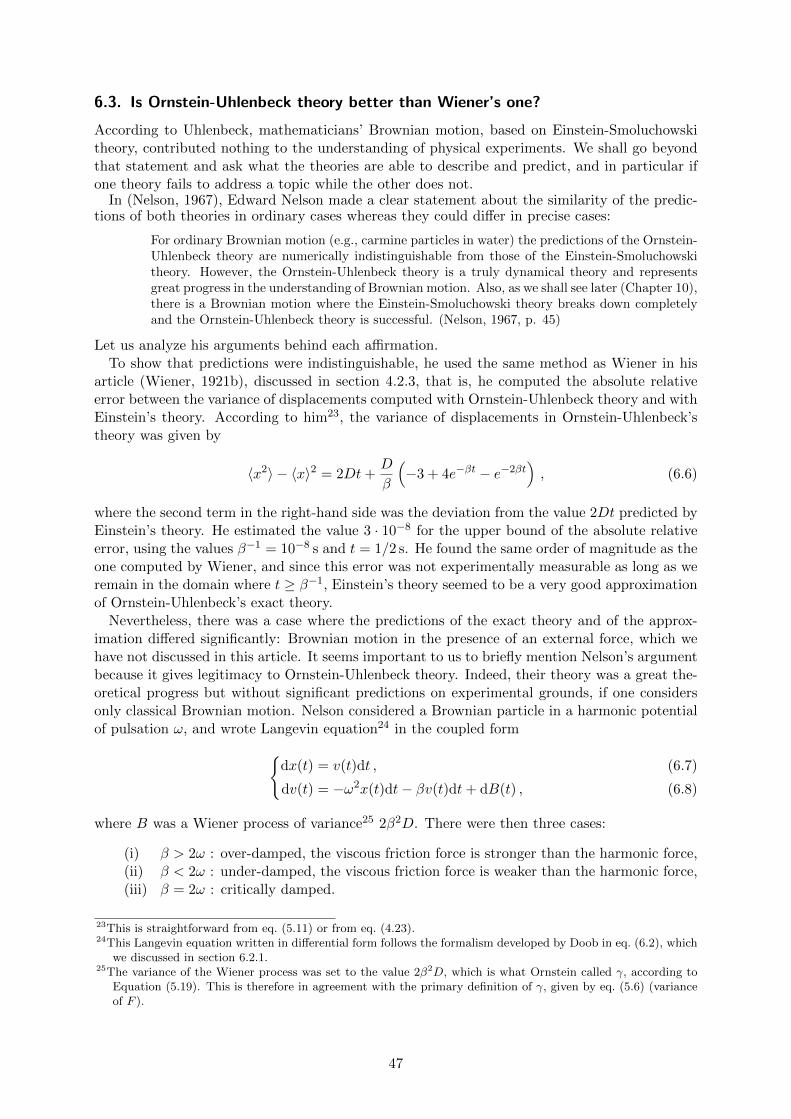
6.3. Is Ornstein-Uhlenbeck theory better than Wiener’s one?

According to Uhlenbeck, mathematicians’ Brownian motion, based on Einstein-Smoluchowskitheory, contributed nothing to the understanding of physical experiments. We shall go beyondthat statement and ask what the theories are able to describe and predict, and in particular ifone theory fails to address a topic while the other does not.

In (Nelson, 1967), Edward Nelson made a clear statement about the similarity of the predic-tions of both theories in ordinary cases whereas they could differ in precise cases:

For ordinary Brownian motion (e.g., carmine particles in water) the predictions of the Ornstein-Uhlenbeck theory are numerically indistinguishable from those of the Einstein-Smoluchowskitheory. However, the Ornstein-Uhlenbeck theory is a truly dynamical theory and representsgreat progress in the understanding of Brownian motion. Also, as we shall see later (Chapter 10),there is a Brownian motion where the Einstein-Smoluchowski theory breaks down completelyand the Ornstein-Uhlenbeck theory is successful. (Nelson, 1967, p. 45)

Let us analyze his arguments behind each affirmation.To show that predictions were indistinguishable, he used the same method as Wiener in his

article (Wiener, 1921b), discussed in section 4.2.3, that is, he computed the absolute relativeerror between the variance of displacements computed with Ornstein-Uhlenbeck theory and withEinstein’s theory. According to him23, the variance of displacements in Ornstein-Uhlenbeck’stheory was given by

〈x2〉 − 〈x〉2 = 2Dt+D

β

(−3 + 4e−βt − e−2βt

), (6.6)

where the second term in the right-hand side was the deviation from the value 2Dt predicted byEinstein’s theory. He estimated the value 3 · 10−8 for the upper bound of the absolute relativeerror, using the values β−1 = 10−8 s and t = 1/2 s. He found the same order of magnitude as theone computed by Wiener, and since this error was not experimentally measurable as long as weremain in the domain where t ≥ β−1, Einstein’s theory seemed to be a very good approximationof Ornstein-Uhlenbeck’s exact theory.

Nevertheless, there was a case where the predictions of the exact theory and of the approx-imation differed significantly: Brownian motion in the presence of an external force, which wehave not discussed in this article. It seems important to us to briefly mention Nelson’s argumentbecause it gives legitimacy to Ornstein-Uhlenbeck theory. Indeed, their theory was a great the-oretical progress but without significant predictions on experimental grounds, if one considersonly classical Brownian motion. Nelson considered a Brownian particle in a harmonic potentialof pulsation ω, and wrote Langevin equation24 in the coupled form{

dx(t) = v(t)dt ,

dv(t) = −ω2x(t)dt− βv(t)dt+ dB(t) ,

(6.7)

(6.8)

where B was a Wiener process of variance25 2β2D. There were then three cases:

(i) β > 2ω : over-damped, the viscous friction force is stronger than the harmonic force,(ii) β < 2ω : under-damped, the viscous friction force is weaker than the harmonic force,(iii) β = 2ω : critically damped.

23This is straightforward from eq. (5.11) or from eq. (4.23).24This Langevin equation written in differential form follows the formalism developed by Doob in eq. (6.2), which

we discussed in section 6.2.1.25The variance of the Wiener process was set to the value 2β2D, which is what Ornstein called γ, according to

Equation (5.19). This is therefore in agreement with the primary definition of γ, given by eq. (5.6) (varianceof F ).

47

This experiment was carried out by Eugen Kappler in 1931 in the three cases. Brownian particleswere small suspended mirrors that were impacted by surrounding gas molecules. This was indeeda one-dimensional Brownian motion, described by the angle that the mirrors made with theirequilibrium positions around their axis, while they were subjected to a torsion force of harmonicform. In case (i) the result was expected to be very close from the Brownian motion of a freeparticle, and therefore Einstein’s approximation was expected to be valid. The plot of the angleversus time in case (i) was very similar to a Wiener trajectory (noisy, random, without a regularpattern), although it never deviated much from its median position because of the torsion force.This was the curve of a Markov process, satisfyingly approximated by a Wiener process, whichis itself Markovian. In case (ii) however, because of the dominance of the harmonic potential,the trajectory was much smoother and approached a sinusoid, which could not be accountedfor by a Markov process. In this case, Einstein-Smoluchowski’s theory, or equivalently Wienerprocesses, failed to account for this experimental behaviour.

7. Conclusion

In this article, we reviewed the history of Brownian motion from Einstein’s first article in 1905to Ornstein’s last article in 1934. We investigated a transition period that has often beenoverlooked, when Brownian motion became an object of interest for mathematicians. Throughthe concept of velocity, we questioned the motivations of the actors during this period, andexplored an aspect of the relationship between physics and mathematics by testing the linksbetween theories. Within this study, we explicated the status of velocity in different Brownianmotion theories, we tackled the birth of stochastic processes and the different ways to introducerandomness into physics, and we presented Wiener’s results in a physicist-friendly way.

Regarding the first physical theories of Brownian motion, we showed that Einstein and Smolu-chowski developed quite similar models in which the notion of displacement was preferred tothat of velocity, which was not properly defined. They introduced stochasticity in their theoriesby considering quantities coming from probability theory, namely probability distributions oraverage quantities. On the contrary, Langevin considered an equation in which velocity ap-peared, and brought randomness into this equation thanks to an additional stochastic force.Those two ways of thinking the stochastic aspect of a problem are still employed today andnamed Fokker-Planck equation and Langevin equation. As long as the time t was not too small,all three theories agreed on the fundamental formula 〈x2〉 ∝ t, which is a consequence of theGaussian distribution of displacements.

We investigated Wiener’s background in order to identify the reasons of his interest for Brow-nian motion, until then a playground for physicists. Wiener’s taste for physics and his awarenessof Brownian motion are partially explained by the readings his Cambridge’s professors suggested.In addition, he found in Brownian motion a good testing ground for his ideas on integrationtheory, which he developed in the light of Perrin’s quotation on the similarity between Browniantrajectories and functions without tangent. He built the first mathematical theory of Brown-ian motion, taking Einstein’s theory as a starting point but knowingly working on an idealizedversion of it, in which the Gaussian distribution discussed above holds at time. This choice ledhim to a proof of the non-differentiability of Brownian trajectories, that is, the non-existence ofBrownian velocities, thus echoing Perrin’s intuition.

Ornstein, later joined by Uhlenbeck, took another road alongside Wiener’s work. WhereasWiener decided to extend Einstein’s Gaussian distribution to short times, Ornstein wanted tocomplement Einstein’s results with a proper treatment of the short time limit that respectedphysical intuition. He chose to work with the velocity, following Langevin’s early calculations.For these two reasons, Wiener’s and Ornstein-Uhlenbeck’s theories were conflicting and yetcomplementary, as confirmed by the modern stochastic calculus initiated by Doob. Ornstein

48

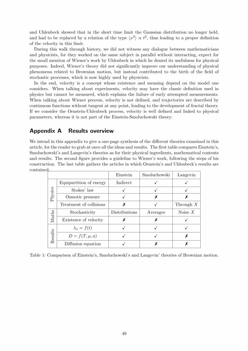
and Uhlenbeck showed that in the short time limit the Gaussian distribution no longer held,and had to be replaced by a relation of the type 〈x2〉 ∝ t2, thus leading to a proper definitionof the velocity in this limit.

During this walk through history, we did not witness any dialogue between mathematiciansand physicists, for they worked on the same subject in parallel without interacting, expect forthe small mention of Wiener’s work by Uhlenbeck in which he denied its usefulness for physicalpurposes. Indeed, Wiener’s theory did not significantly improve our understanding of physicalphenomena related to Brownian motion, but instead contributed to the birth of the field ofstochastic processes, which is now highly used by physicists.

In the end, velocity is a concept whose existence and meaning depend on the model oneconsiders. When talking about experiments, velocity may have the classic definition used inphysics but cannot be measured, which explains the failure of early attempted measurements.When talking about Wiener process, velocity is not defined, and trajectories are described bycontinuous functions without tangent at any point, leading to the development of fractal theory.If we consider the Ornstein-Uhlenbeck process, velocity is well defined and linked to physicalparameters, whereas it is not part of the Einstein-Smoluchowski theory.

Appendix A Results overview

We intend in this appendix to give a one-page synthesis of the different theories examined in thisarticle, for the reader to grab at once all the ideas and results. The first table compares Einstein’s,Smoluchowski’s and Langevin’s theories as for their physical ingredients, mathematical contentsand results. The second figure provides a guideline to Wiener’s work, following the steps of hisconstruction. The last table gathers the articles in which Ornstein’s and Uhlenbeck’s results arecontained.

Einstein Smoluchowski Langevin

Physi

cs

Equipartition of energy Indirect X X

Stokes’ law X X X

Osmotic pressure X 7 7

Treatment of collisions 7 X Through X

Mat

hs Stochasticity Distributions Averages Noise X

Existence of velocity 7 7 X

Res

ult

s λx = f(t) X X X

D = f(T, µ, a) X X 7

Diffusion equation X 7 7

Table 1: Comparison of Einstein’s, Smoluchowski’s and Langevin’ theories of Brownian motion.

49

1920

1921a 1921b

1922 1930

1923 1933

Axiomatic integration

Wiener measure

Lebesguemeasure

Einstein'sformula

Figure 3: Guide to Wiener’s work. The seven articles are split into the four stages of Wiener’sconstruction, and the ideas continuity from an article to an other is symbolised byarrows.

〈q〉 〈q2〉 〈qk〉, k ≥ 3 f(q, q0, t) Fokker-Planck equation

q = x 1917 (O) 1917 (O) 1930 (O, U) 1930 (O, U) 1934 (O, W)

q = v 1917 (O) 1917 (O) 1930 (O, U) 1930 (O, U) 1917 (O)

Table 2: Summary of Ornstein’s and Uhlenbeck’s main results. Each box contains the year andthe authors (O : Ornstein, U : Uhlenbeck, W : van Wijk) of the article in which theresult appearing in the first line is derived.

References

Bachelier, L. (1900). Theorie de la speculation. Annales scientifiques de l’Ecole normale superieure17, pp. 21–86.

Brush, S. (1976). The kind of motion we call heat. North Holland publishing Company. Amster-dam, New York, Oxford.

Chaudesaigues, J. U. (1908). Le mouvement Brownien et la formule d’Einstein. Comptes rendusde l’academie des sciences de Paris, pp. 1044–1046.

Cohen, E. G. D. (1990). George E. Uhlenbeck and statistical mechanics. American Journal ofPhysics 58.(7), pp. 619–625.

Darrigol, O. (2018). Atoms, Mechanics, and Probability: Ludwig Boltzmann’s Statistico-MechanicalWritings - An Exegesis. Oxford University Press. Oxford, New York.

Dimand, R. W. (1993). The case of Brownian motion: a note on Bachelier’s contribution. TheBritish Journal for the History of Science 26.(2), pp. 233–234.

Doob, J. L. (1942). The Brownian Movement and Stochastic Equations. The Annals of Mathe-matics 43.(2), pp. 351–369.

(1966). Wiener’s work in probability theory. Bulletin of the American Mathematical So-ciety 72.(1), pp. 69–73.

50

Dresden, M. (1989). George E. Uhlenbeck. Physics Today 42.(12), pp. 91–94.

Duclaux, J. (1908). Pressions osmotiques et mouvement brownien. Comptes rendus de l’academiedes sciences de Paris, pp. 131–134.

Duplantier, B. (2006). Brownian Motion, “Diverse and Undulating”. Einstein, 1905–2005: PoincareSeminar 2005. Damour, Thibault and Darrigol, Olivier and Duplantier, Bertrand and Ri-vasseau, Vincent. Basel: Birkhauser Basel, pp. 201–293.

(2007). Brownian Motion, ”Diverse and Undulating”. arXiv:0705.1951.

Einstein, A. (1905). Uber die von der molekularkinetischen Theorie der Warme geforderte Bewe-gung von in ruhenden Flussigkeiten suspendierten Teilchen. Annalen der Physik 17.(4),pp. 549–560. Translated in english in Investigations, p. 1-18.

(1906). Zur Theorie der Brownschen Bewegung. Annalen der Physik 19.(4), pp. 371–381.Translated in english in Investigations, p. 19-35.

(1907). Theoretische Bemerkungen uber die Brownsche Bewegung. Zeitschrift fur Elek-trochemie und angewandte physikalische Chemie 13, pp. 41–42. Translated in english inInvestigations, p. 63-67.

(1926). Investigations on the Theory of the Brownian Movement. Dover Publications, Inc.New-York. 1956 (english translation). Abbreviated Investigations.

Getoor, R. (2009). J. L. Doob: Foundations of stochastic processes and probabilistic potentialtheory. The Annals of Probability 37.(5), pp. 1647–1663.

Henri, V. (1908a). Etude cinematographique des mouvements browniens. Comptes rendus del’academie des sciences de Paris, pp. 1024–1026.

(1908b). Influences des milieux sur les mouvements browniens. Comptes rendus de l’academiedes sciences de Paris, pp. 62–65.

Home, R. (2005). Speculating about Atoms in Early 20th-century Melbourne: William Suther-land and the Sutherland-Einstein Diffusion Relation, Sutherland Lecture. 16th NationalCongress. 16th National Congress. Australian Institute of Physics, Canberra.

Kahane, J.-P. (1998). Un essai sur les origines de la theorie mathematique. Societe Mathematiquede France 1998, pp. 123–155.

(2014). Paul Langevin, le mouvement brownien et l’apparition du bruit blanc. Un texte,un mathematicien. Bibliotheque Nationale de France.

Kerker, M. (1976). The Svedberg and Molecular Reality. Isis 67.(2), pp. 190–216.

Langevin, P. (1908). Sur la theorie du mouvement Brownien. Comptes rendus de l’academie dessciences de Paris, pp. 530–533.

Levy, P. (1922). Lecons d’analyse fonctionnelle. Gauthier-Villars et Cie, Editeurs. Paris.

Maiocchi, R. (1990). The case of Brownian motion. The British Journal for the History of Science23.(3), pp. 257–283.

Masani, P. R. (1990). Norbert Wiener 1894-1964. Birkhauser Basel. Basel.

Mason, R. C. (1945). Leonard Salomon Ornstein. Science 102.(2660), pp. 638–639.

Naqvi, K. R. (2005). The origin of the Langevin equation and the calculation of the mean squareddisplacement: Let’s set the record straight. arXiv:physics/0502141. arXiv: physics /

0502141.

Nelson, E. (1967). Dynamical Theories of Brownian Motion. Princeton University Press. url:https://web.math.princeton.edu/~nelson/books/bmotion.pdf.

51

Nye, M. J. (1972). Molecular Reality. A Perspective on the Scientific Work of Jean Perrin.Elsevier. New York.

Ornstein, L. (1919). On the Brownian Motion. KNAW, Proceedings 21, pp. 96–108.

Ornstein, L. and W. R. V. Wijk (1934). On the derivation of distribution functions in problemsof Brownian motion. Physica 1, pp. 235–254.

Ornstein, L. and F. Zernike (1919). The Theory of the Brownian Motion and Statistical Me-chanics. KNAW, Proceedings 21, pp. 109–114.

Paley, R. E. A. C., N. Wiener, and A. Zygmund (1933). Notes on random functions. Mathema-tische Zeitschrift 37.(1), pp. 647–668.

Perrin, J. (1908a). L’agitation moleculaire et le mouvement Brownien. Comptes rendus del’academie des sciences de Paris, pp. 967–970.

(1908b). La loi de Stokes et le mouvement Brownien. Comptes rendus de l’academie dessciences de Paris, pp. 475–476.

(1909). Mouvement brownien et realite moleculaire. Masson et Cie, Editeurs. Paris.

(1913). Les Atomes. Flammarion. Paris. (2014).

Piasecki, J. (2007). Centenary of Marian Smoluchowski’s theory of Brownian Motion. ActaPhisica Polonica B 38.(5), pp. 1623–1629.

Pohl, G. (2006). The theory of Brownian motion — one hundred years old. The Global and theLocal: The History of Science and the Cultural Integration of Europe. Proceedings of the2nd ICESHS. Cracow, pp. 419–424.

Renn, J. (2005). Einstein’s invention of Brownian motion. Annalen der Physik 14 (S1), pp. 23–37.

Ryskin, G. (1997). Simple procedure for correcting equations of evolution: Application to Markovprocesses. Physical Review E 56.(5), pp. 5123–5127.

Smoluchowski, M. (1906). Essai d’une theorie cinetique du mouvement Brownien et des milieuxtroubles. Bulletin International de l’Academie des sciences de Cracovie, pp. 577–602.

Sredniawa, B. (1992). The Collaboration of Marian Smoluchowski and Theodor Svedberg onBrownian Motion and Density Fluctuations. Centaurus 35.(3), pp. 325–355.

Svedberg, T. (1906a). Uber die Eigenbewegung der Teilchen in Kolloidalen Losungen. Zeitschriftfur Elektrotechnik und Elektrochemie 12.(47), pp. 853–860.

(1906b). Uber die Eigenbewegung der Teilchen in Kolloidalen Losungen II. Zeitschrift furElektrotechnik und Elektrochemie 12.(51), pp. 909–910.

Uhlenbeck, G. and L. Ornstein (1930). On the Theory of the Brownian Motion. Physical Review36.(5), pp. 823–841.

Uhlenbeck, G. and M. C. Wang (1945). On the Theory of the Brownian Motion II. Reviews ofModern Physics 17.(2), pp. 323–342.

Wiener, N. (1920). The Mean of a Functional of Arbitrary Elements. The Annals of Mathematics22.(2), pp. 66–72.

(1921a). The average of an analytical functional. Proceedings of the National Academy ofSciences (7), pp. 253–260.

(1921b). The Average of an Analytic Functional and the Brownian Movement. Proceedingsof the National Academy of Sciences 7.(10), pp. 294–298.

52

Wiener, N. (1922). The Average value of a functional. Proceedings of the London MathematicalSociety 22, pp. 454–467.

(1923). Differential Space. Journal of Mathematics and Physics 2.(1), pp. 131–174.

(1930). Generalized harmonic analysis. Acta Mathematica 55, pp. 117–258.

(1956). I Am A Mathematician The Later Life of a Prodigy. The M.I.T Press. Cambridge,Massachussetts.

53